Discrete signal quantization

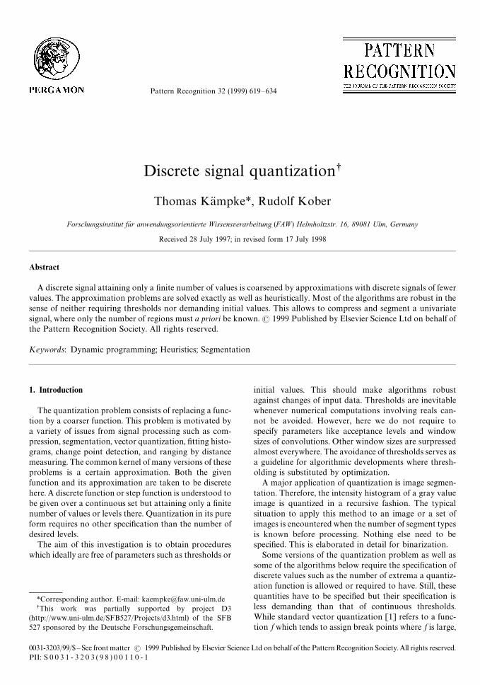
Pattern Recognition 32 (1999) 619—634

Discrete signal quantizations

Thomas Kampke*, Rudolf Kober

Forschungsinstitut fur anwendungsorientierte Wissensverarbeitung (FAW) Helmholtzstr. 16, 89081 Ulm, Germany

Received 28 July 1997; in revised form 17 July 1998

Abstract

A discrete signal attaining only a finite number of values is coarsened by approximations with discrete signals of fewervalues. The approximation problems are solved exactly as well as heuristically. Most of the algorithms are robust in thesense of neither requiring thresholds nor demanding initial values. This allows to compress and segment a univariatesignal, where only the number of regions must a priori be known. ( 1999 Published by Elsevier Science Ltd on behalf ofthe Pattern Recognition Society. All rights reserved.

Keywords: Dynamic programming; Heuristics; Segmentation

1. Introduction

The quantization problem consists of replacing a func-tion by a coarser function. This problem is motivated bya variety of issues from signal processing such as com-pression, segmentation, vector quantization, fitting histo-grams, change point detection, and ranging by distancemeasuring. The common kernel of many versions of theseproblems is a certain approximation. Both the givenfunction and its approximation are taken to be discretehere. A discrete function or step function is understood tobe given over a continuous set but attaining only a finitenumber of values or levels there. Quantization in its pureform requires no other specification than the number ofdesired levels.

The aim of this investigation is to obtain procedureswhich ideally are free of parameters such as thresholds or

*Corresponding author. E-mail: [email protected] work was partially supported by project D3

(http://www.uni-ulm.de/SFB527/Projects/d3.html) of the SFB527 sponsored by the Deutsche Forschungsgemeinschaft.

initial values. This should make algorithms robustagainst changes of input data. Thresholds are inevitablewhenever numerical computations involving reals can-not be avoided. However, here we do not require tospecify parameters like acceptance levels and windowsizes of convolutions. Other window sizes are surpressedalmost everywhere. The avoidance of thresholds serves asa guideline for algorithmic developments where thresh-olding is substituted by optimization.

A major application of quantization is image segmen-tation. Therefore, the intensity histogram of a gray valueimage is quantized in a recursive fashion. The typicalsituation to apply this method to an image or a set ofimages is encountered when the number of segment typesis known before processing. Nothing else need to bespecified. This is elaborated in detail for binarization.

Some versions of the quantization problem as well assome of the algorithms below require the specification ofdiscrete values such as the number of extrema a quantiz-ation function is allowed or required to have. Still, thesequantities have to be specified but their specification isless demanding than that of continuous thresholds.While standard vector quantization [1] refers to a func-tion f which tends to assign break points where f is large,

0031-3203/99/$—See front matter ( 1999 Published by Elsevier Science Ltd on behalf of the Pattern Recognition Society. All rights reserved.PII: S 0 0 3 1 - 3 2 0 3 ( 9 8 ) 0 0 1 1 0 - 1

Fig. 1. Discrete function f (bold) and a quantization s5.

the current type of quantization tends to assign breakpoints where the change of f is large. This yields a nonlin-ear optimisation problem, because both levels and breakpoints of the quantization function have to be deter-mined simultaneously. The current approximation prob-lem originated with almost no modification from issuesof tracking vessels in computer tomograms [2, 3] and bywork on adaptively encoding various classes of images[4, 5]. Quantization functions here are chosen to be ofa simpler type than those of the theoretical investigationsfor the two-dimensional signals given in [6—8].

Within optimization techniques we mainly resort todynamic programming. Value iteration is feasible herebecause the horizons of the dynamic programs are finite.Though this leads to a polynomial algorithm even fasteralgorithms for approximate optimal fitting are de-veloped. These are search techniques based on variousnotions of locality.

The quantization problem must not be confused withtime warping. The latter [9] requires that two givensignals be aligned where certain deformations on the timescale are allowed. Quantization leaves one signal fixedwhile constructing the other.

The remainder of this paper is organized as follows.The general quantization problem and two of its vari-ations are introduced in Section 2. Section 3 providesexact and Section 4 provides approximate algorithms forall cases. Section 5 contains procedures on adaptive com-putations of the number of segments into which a givensignal should be segmented if this information is notgiven otherwise. Section 6 contains some large examplesincluding a segmentation problem from optical inspec-tion of printed circuit boards. Section 7 concludes thiswork giving a short perspective. All subsections from 3.2onwards and Sections 4 and 5 can be skipped withoutomitting material which is essential to image segmenta-tion. :" and :8 denote a definition, DAD indicates thecardinality of a set A, and e will mark the end of anargument.

2. Quantization

Quantization can be investigated for various types offunctions. In contrast to the continuous case [10], func-tions here are taken from the set Sl which is supposed tocontain all step functions over an interval [a, b] of realswhere the step functions attain at most l!1 values. Toavoid trivial complications, functions from Sl are as-sumed to be proper meaning that adjacent levels aredifferent unless stated otherwise. All adjacent intervals off with same value combined are called level segment.For f"+N~1

i/1vi1(wi, wi`1)

with indicator function1A(x)"1 for x3A and I

A(x)"0 for x NA, the interior

break points are summarized in set ¼"Mw2,2 ,

wN~1

N. The bounding break points w1

and wN

are impli-

citly included in break point considerations on someoccasions. The range of values attained by f is denoted byran( f ). The distance of two integrable functions g

1, g

2over [a, b] will be inferred from the standard 2-norm

E g1! g

2E

2" E g

1! g

2E"J :b

a(g

1(x)!g

2(x))2 dx.

Values of step functions at break points do not effect thenorm so they usually will be ignored. An optimal quant-ization of f3S

Nwith respect to S

n, 2)n(N, is defined

to be a function s0n3S such that s0

n"argmin

sn|SnE f!s

nE.

A discrete signal and a quantization are shown inFig. 1. The distance E f!s

nE is the quantization error

of snfor f.

Break points of the optimal quantization need only besearched in the set of interior break points of f [11]. Animmediate consequence is that the quantization problemis in P for fixed n and fixed N!n. Later it will be shownthat the quantization problem is in P for eachn3M2,2 , N!1N. The computation of all quantizationswith each reasonable number of levels n"2,2, N!1can also be facilitated in polynomial time.

It will be essential to many constructions that oncea partition a"x

1(2(x

n"b is fixed, the best pos-

sible quantization sn,0

"+n~1i/1

yi,0

1(xi, xi`1)

is given byyi,0

:"y(xi, x

i`1):"1/(x

i`1!x

i) :xi`1

xif (u) du, see [Lemma

2.2] [11]. The squared quantization error for a partition isthen k(x

2,2 , x

n~1):"k

f(x

2,2 , x

n~1):"E f!s

n,0E2"

+n~1i/1

:xi`1xi

( f (x)!y (xi, x

i`1))2 dx. For any fixed parti-

tion the best possible quantization sn,0

can be computedin O(N).

Optimal quantization is essentially uneffected by somealterations of f. For example, the partition of an optimalquantization is not changed if f is lifted to become f#cor reflected to become f!2( f!c) for any real c. Thefirst implies that values from f can be assumed to benon-negative.

Quantization need not preserve shape features likesymmetry. A function f with f ((a#b)/2!x)#f ((a#b)/2#x)"f ((a#b)/2) for all x3[0, (b!a)/2]need not impose this point symmetry to any of its opti-mal quantizations. The same applies to reflective func-tions. i.e. to functions with f ((a#b)/2!x)"f ((a#b)/2#x) for all x3[0, (b!a)/2].

620 T. Ka(mpke, R. Kober / Pattern Recognition 32 (1999) 619—634

Several variations and a refinement of the quantizationproblem are also considered. One variation stipulatedthat quantization functions have a restricted range. Thismeans that ran(s

n)-E, where E is some fixed and finite

set of reals. A particularly appealing choice for E isE"ran( f ). A further specialization is binary quantiz-ation meaning that E"M0. 1N.

Another type of quantization results from identifyingisolated segments. ‘‘Interesting’’ parts of f are consideredto be relatively long segments where the function isconstant or ‘‘approximately’’ constant but all other seg-ments of the function do not matter. Finding the interest-ing regions will be reduced to fitting partially defined stepfunctions being denoted as subquantizations. These do-main restrictions complement the foregoing range re-strictions.

Finally, quantization is performed in a two phasemode. In the first phase the quantization functions re-ceive an increasing number of levels until a desired num-ber of local extrema is reached. This allows to identifyone or several regions which the second phase focuses on.The quantization functions there receive an increasingnumber of levels until again a certain pattern of localextrema is reached. This leads to a robust segmentationof the original signal in terms of peak regions whichextend from a local minimum to an adjacent local min-imum.

3. Exact algorithms

3.1. General problem

The quantization problem can be solved exactly bya dynamic program which is derived from the computa-tion of cheapest paths with fixed number of arcs indirected graphs [11]. An arc (i, j ) with 1)i(j)N istherefore assigned cost c

ij:":wj

wi( f (x)!y(w

i, w

j))2 dx.

Also, for later use the cost coefficients cii:"0 are defined

for 1)i)N. The upper triangular matrix of all O (N2)cost coefficients can be computed in O(N2). The cost ofa cheapest path from w

ito w

Nhaving exactly k intermedi-

ate break points is denoted by Ci(k). The C

i(k) can be

computed iteratively.

A1. (Initialization). C

i(0)"c

iNi"2,2 , N!1, l(0)"c

1N.

2. (Iteration). For k"1,2 , n!2 do:(a) Computation of the value of a cheapest path from

1 to N with exactly k intermediate vertices

mini/2,2 ,N~k

c1i#C

i(k!1)"l(k),

argmini/2,2 ,N~k

c1i#C

i(k!1)"p

1(k).

(b) Value update for insertion of one additional inter-mediate point

Ci(k)" min

j/i`1,2 ,N~k

cij#C

j(k!1),

argminj/i`1,2 ,N~k

cij#C

j(k!1)"p(i, k)

for i"2,2 , N!(k#1).

The procedure terminates with optimal quantization er-

rors E f!s02E"Jl(0),2 ,E f!s0

nE"Jl(n!2). The

partitions of global optimal quantizations with up ton!1 levels can be found by tracing the pointers pand p

1. The quantization s0

nresults from break points

at positions p*(n!2),2 , p*(1) in ¼, wherep*(n!2):"p

1(n!2), p*(n!2!1):"p (p*(n!2),

n!2!1),2 , p*(1) :"p(p* (2), 1). In case of ties forp1(k) and p(i, k) the selection of the smallest minimizing

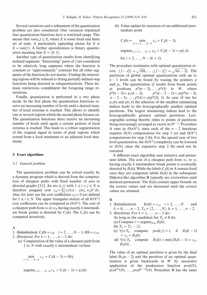
indices leads to the lexicographically smallest optimalpartitions. The largest minimizing indices lead to thelexicographically greatest optimal partitions. Lexi-cographic sorting thereby refers to points of partitionsbeing increasingly arranged as vector in Rn~2. ProcedureA runs in O(nN2), since each of the n!2 iterationsrequires O(N) computations for step 2 (a) and O(N2)computations for step 2 (b). For the special case of twolevel quantization, the O(N2 ) complexity can be loweredto O(N), since the expensive step 2 (b) need not beexecuted.

A different exact algorithm uses tentative and perma-nent labels. The cost of a cheapest path from w

1to w

ihaving exactly k intermediate break points is eventuallydenoted by D

i(k). While the labels C

i(k) in A remain fixed

once they are computed, labels Di(k) in the subsequent

Dijkstra-like algorithm B typically are overwritten untildeclared permanent. The D

i(k) contain upper bounds on

the correct values and are decreased until the correctvalues are attained.

B1. (Initialization). D

i(k)"c

1i, i"2,2 , N and

k"0,2 , n!2, ¹k"M2,2 , NN, k"1,2 , n!2.

2. (Iteration). For k"1,2 , n!2 do:As long as the candidate list ¹

kO0 do:

(a) Compute i"argminj|Tk

Dj(k).

(b) ¹k"¹

k!MiN.

(c) ∀j3¹k

compute pred( j )"i, if Di(k!1)

#cij(D

j(k).

(d) ∀j3¹k

compute Dj(k)"minMD

i(k!1)#c

ij,

Dj(k)N.

The value of an optimal partition is given by the finallabel D

N(n!2) and the partition of an optimal quan-

tization is given backwards in ¼ by successiveapplication of the predecessor function pred (N),pred(2)(N),2 , pred(n~2)(N). Procedure B has the same

T. Ka(mpke, R. Kober / Pattern Recognition 32 (1999) 619—634 621

O(nN2 ) complexity as procedure A. The particular coststructure here implies that i"argmin

j|TkD

j(k)"

min ¹kin step 2(a).

3.2. Restricted range

Quantization functions are now restricted to attainvalues in some finite set E-R. A typical but not the onlyreasonable choice is E"ran( f ) so that the quantizationis guaranteed to attain only values which f has. In con-trast to the case of signals f and quantizations s

nwith

unrestricted range, the optimal quantization now neednot be a proper function from S

neven if f is a proper

function from SN. Moreover, restriction of an optimal

quantization may differ from an optimal restrictedquantization, as illustrated already for the binary casebelow.

The dynamic program A and its variant B are applic-able to quantization with restricted range when thecost coefficients are modified to become c

ij:"

:wjwi

( f (x)!c)2 dx, where c"argmine|E

Dy(wi, w

j)!eD.

This is due to the best choice of a single quantizationlevel over the fixed interval (w

i, w

j) being a minimizer of

Pwj

wi

( f (x)!e)2 dx"Pwj

wi

f (x)2 dx!2e Pwj

wi

f (x) dx

#e2(wj!w

i).

As the latter is a convex parabola in e, the best choice fore is one closest to the global minimizer y (w

i, w

j). The

complexity of this computation is O(logDE D), if the setE receives an O(DEDlogDE D) preprocessing for structuringit as a heap. For E"ran ( f ) this results in DED"O(N)and thus in the worst case complexityO(N2 logN2 )#O (n)N2)"O(maxMn, log NN )N2 ) for al-gorithms A and B with range restriction.

3.3. Binary problem

As a special case of range restriction, function f issupposed to be binary and s

nis restricted to be binary,

too, i.e. ran ( f )"ran(sn)"M0, 1)":E. Binary quantiz-

ation functions are denoted sn, bin

"+n~1i/1

yi,bin

1(xi, xi`1)

and optimal binary levels for a fixed partition are givenby

yi,0,bin

:"ybin

(xi, x

i`1):"argmax

u|M0, 1N

j( f"u over [xi, x

i`1]),

where j is the Lebesgue measure. Costs are given byC

i, j,bin:"minMj ( f"1 over [w

i, w

j]), j ( f"0 over

[wi, w

j])N. The subsequent obvious fact relates the gen-

eral with the binary case for a fixed partitiona"x

1(2(x

n"b. The inequality y(x

i, x

i`1)(1

2im-

plies y"*/

(xi, x

i`1)"0 and y (x

i, x

i`1)'1

2implies

y"*/

(xi, x

i`1)"1, where the implications can be reversed

if equality is allowed. Level yi,0

"1/2 is ambiguous in thebinary case. Moreover, E f!s

n,0,binE2)1

2(b!a) for

sn,0,bin

"+n~1i/1

ybin

(xi, x

i`1) 1

(xi, xi`1)with arbitrary given

partition.Binarizing an optimal quantization of a binary func-

tion does not necessarily lead to an optimal binaryquantization.

Example 1. A six level binary function is considered with

f (x)"

1 if x3(0, 3),0 if x3(3, 4),1 if x3(4, 6),0 if x3(6, 7),1 if x3(7, 8),0 if x3(8, 10).

The optimal two level quantization is uniquely given bybreak point x0

2"w

6"8, while the two binary quantiz-

ations with break points x02,bin

"w4"6 and

x02,bin

"w6"8 are optimal.

Distorting the break point w6

to w6"8!e with

0(e(12

and keeping all other break points fixedpreserves optimality of the general quantization withbreak point x0

2"8!e. Optimality of the binary quantiz-

ation with the same partition is destroyed. Only thebinary quantization with break point x0

2,"*/"6 is now

optimal.

Procedures A and B with binary cost coefficients andbinary levels yield optimal binary quantizations. Thecomplexity of A and B is not reduced when applied tobinary instead of general quantization.

3.4. Subquantization

In a variation of the general quantization problem, thesignal f is now analyzed for having n intervals I

1,2 , I

nwhich are ‘‘large’’ and ‘‘important’’ compared to the re-maining level segments. Each interval I

imay consist of

several level segments to account for outliers and ‘‘unim-portant’’ changes in the values of f.

A set R"MR1,2 , R

nN of pairwise disjoint intervals

with R"R1X2XR

n-(a, b) is called subpartition of

(a, b). A subpartition induces a subquantization which isa step function s

n,Rpartially defined on dom( f ), where

sn,R

(x)"GyRi:"1/j (R

i) ) :

Rif (u) du if x3R

i,

undefined if x3(a, b)!R.

A subquantization induced by I"MI1,2 , I

nN which

solves the minimization over all subpartitions

E f!sn,I

E#j((a, b)!I )"minsm, R

E f!sn,R

E

#j((a, b)!R)


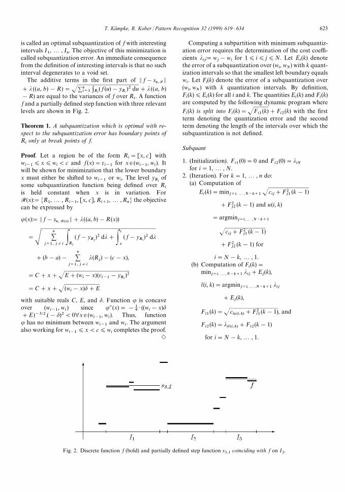
Fig. 2. Discrete function f (bold) and partially defined step function s3,I

coinciding with f on I2.

is called an optimal subquantization of f with interestingintervals I

1,2 , I

n. The objective of this minimization is

called subquantization error. An immediate consequencefrom the definition of interesting intervals is that no suchinterval degenerates to a void set.

The additive terms in the first part of E f!sn,R

E#j ((a, b)!R)"J+n

i/1:Ri

( f (u)!yRi

)2 du#j ((a, b)!R) are equal to the variances of f over R

i. A function

f and a partially defined step function with three relevantlevels are shown in Fig. 2.

Theorem 1. A subquantization which is optimal with re-spect to the subquantization error has boundary points ofR

ionly at break points of f.

Proof. Let a region be of the form Ri"[x, c] with

wi~1

)x)wi(c and f (x)"v

i~1for x3(w

i~1, w

i). It

will be shown for minimization that the lower boundaryx must either be shifted to w

i~1or w

i. The level y

Riof

some subquantization function being defined over Ri

is held constant when x is in variation. ForR(x):"MR

1,2 , R

i~1, [x, c], R

i`1,2 , R

nN the objective

can be expressed by

u(x):"E f!sn, R(x)

E#j ((a, b)!R(x))

"Sn+

j/1, jOiPRj

( f!yRj

)2 dj#Pc

x

( f!yRi

)2 dj

#(b!a)!n+

j/1, jOi

j (Rj)!(c!x),

"C#x#JE#(wi!x)(v

i~1!y

Ri)2

"C#x#J(wi!x)d#E

with suitable reals C, E, and d. Function u is concaveover (w

i~1, w

i) since uA (x)"!1

4) ((w

i!x)d

#E)~3@2.(!d)2(0∀x3(wi~1

, wi). Thus, function

u has no minimum between wi~1

and wi. The argument

also working for wi~1

)x(c)wicompletes the proof.

e

Computing a subpartition with minimum subquantiz-ation error requires the determination of the cost coeffi-cients j

ij:"w

j!w

ifor 1)i)j)N. Let E

i(k) denote

the error of a subquantization over (wi, w

N) with k quant-

ization intervals so that the smallest left boundary equalswi. Let F

i(k) denote the error of a subquantization over

(wi, w

N) with k quantization intervals. By definition,

Fi(k))E

i(k) for all i and k. The quantities E

i(k) and F

i(k)

are computed by the following dynamic program where

Fi(k) is split into F

i(k)"JF

i1(k)#F

i2(k) with the first

term denoting the quantization error and the secondterm denoting the length of the intervals over which thesubquantization is not defined.

Subquant

1. (Initialization). Fi1

(0)"0 and Fi2

(0)"jiN

for i"1,2 , N.2. (Iteration). For k"1,2 , n do:

(a) Computation of

Ei(k)"min

j/i, 2 ,N~k`1Jc

ij#F2

j1(k!1)

#F2j2

(k!1) and u (i, k)

"argminj/i,2 ,N~k`1

Jcij#F2

j1(k!1)

#F2j2

(k!1) for

i"N!k,2 , 1.(b) Computation of F

i(k)"

minj/i,2 ,N~k`1

jij#E

j(k),

l (i, k)"argminj/i,2 ,N~k`1

jij

#Ej(k),

Fi1

(k)"Jciu (i,k)

#F2i1

(k!1), and

Fi2

(k)"jil (i,k)

#Fi2

(k!1)

for i"N!k,2 , 1.


The procedure terminates with optimal subquantizationerror F

1(n). The interesting intervals can be traced

to positions of break points of f with the followingindices: p*(n):"l (1, n), q*(n):"u(p*(n), n), p*(n!1):"l(q*(n), n!1), q*(n!1):"u(p*(n!1), n!1),2 ,p*(1):"l(q* (2), 1), q*(1):"u (p*(1), 1). This means thatI1"(w

p* (n), w

q*(n)),2 , I

n"(w

p* (1), w

q*(1)). The proced-

ure Subquant runs in O(nN2 ).Another criterion for subquantization is the subvari-

ation error

minR1

,2 ,Rn

n+i/1

Var f (Ri)#j((a, b)!R),

where R"MR1,2 , R

nN is a subpartition of (a, b) and

Var f (Ri) is the total variation of f over R

i. A similar

result as Theorem 1 also applies to the subvariationerror. Furthermore, the dynamic program Subquant forminimizing the subquantization error carries over to thesubvariation error, where the cost c

ijis replaced by

vij:"+j

k/i`1Dvk!v

k~1D, if 1)i(j)N and v

ij:"0 if

1)i"j)N.

Subvar1. (Initialization). F

i(0)"j

iNfor i"1,2 , N.

2. (Iteration). For k"1,2 , n do:(a) Computation of E

i(k)"min

j/i,2 ,N~k`1vij

#Fj(k!1) and u (i, k)"argmin

j/i,2 ,N~k`1vij

#Fj(k!1) for i"N!k,2 , 1.

(b) Computation of Fi(k)"min

j/i,2 ,N~k`1jij

#Ej(k) and l(i, k)"argmin

j/i,2 ,N~k`1jij

#Ej(k) for i"N!k,2 , 1.

4. Approximate algorithms

Though all versions of the quantization problem canbe solved to optimality with polynomial effort, approxi-mating heuristics running even faster are presented. Thereason is that the ‘‘cubic’’ run time O(nN2) may alreadybe prohibitive in certain situations.

4.1. General quantization

Heuristic algorithms for the general quantizationproblem are now introduced in an order which roughlycorresponds to decreasing worst case complexity.

Dynamic programming is now deviced to yield heuris-tic solutions only which will reduce the runtime com-pared to procedure A. This runtime is due to the dynamicprogram being prevented from searches over long inter-vals. Therefore, the domain [a, b] is partitioned inton!2 intervals I

1,2 , I

n~2which are balanced meaning

that each interval contains xN/(n!2)y or vN/(n!2)wbreak points of f. The intervals I

iare sometimes

identified with the set of indices of those wjwhich belong

to Ii.

Only quantizations of f are now considered whichhave exactly one break point in each of the given inter-vals—except break points a and b. The dynamic programA thus results in the subsequent partition procedure P. Itcomputes the values D*

i(s) which denote the cost of

a cheapest path from w1

to wi3I

s`1with s intermediate

break points, one in each of the intervals I1,2 , I

s,

s3M1,2 , n!3N.

P1. (Initialization). Computation of D*

i(0)"c

1ifor all

i3I1

and l (0)"c1N

.2. (Iteration). For k"1,2 , n!2 do:

(a) Computation of cji

for all j3Ik, i3I

k`1and c

jNfor all j3I

k.

(b) Computation of minj|Ik

D*j(k!1)#c

jN"l(k)

and argminj|Ik

D*j(k!1)#c

jN"p

1(k).

(c) Computation of updates for insertionof one additional intermediate point D*

i(k)

"minj|Ik

D*j(k!1)#c

jiand

argminj|Ik

D*j(k!1)#c

ji"p(i, k) for i3I

k`1,

if k#1)n!2. No computation for k"n!2.

The construction of the best quantization found by P fol-lows the same trace through p

1and p as for algorithm A.

Procedure P requires O(DIiD2 ) computations for each

iteration of step 2(a) and 2(c), and O(DIiD) for each iteration

of step 2(b). The overall complexity of P isO((n!2)DI

iD2)"O(N2/n), since xN/(n!2)y

)DIiD)vN/(n!2)w for all I

i.

Computing all necessary cost coefficients for the exactdynamic program A requires O (N2) which is strictly lessthan the complexity O(nN2) of A itself. The approximatedynamic program P is of an equally balanced complexityfor computing the involved cost coefficients and the op-timization.

Another heuristic approach is based on crawlingthrough the break point set ¼. For a vector of breakpoints (x

2,2 , x

n~1) the set of one step neighbours to the

right N(x2,2 , xn~1)`

is the set of all vectors of breakpoints which differ in only one coordinate from x; thatcoordinate is different from all other coordinates of and itlies in ¼ adjacent to the right of the differing coordinatevalue: N

(x2,2 , xn~1)`:"MyDy"(y

2,2 , y

n~1)3¼n~2

such that xi"y

ifor all i3M2,2 , n!1N!Mi

0N where

xi0"w

k(w

k`1"y

i0Ox

ifor all i3M1,2 , nN and suit-

able kN.

C1. (Initialization). Set x

2"w

2,2 , x

n~1"¼

n~1,

¸"M(x2,2 , x

n~1)N, F"k(x

2,2 , x

n~1).


Table 1

Algorithm Solution type Remark Complexity

A Exact n exact O(nN2)B Exact n exact O(nN2)P Approximate n exact O(N2/n)C Approximate n exact O(n2N)S Approximate n exact O(nN)Binarysearch

Approximate napproximate

O(N log N)

2. (Iteration). Repeat until x2"w

N~(n~2),2 , x

n~2"w

N~2, x

n~1"w

N~1:

(a) Computation of z"argminy|N(x2

,2 , xn~1)`k(y),

where z"(x2,2 , x

i~1, y

i, x

i`1,2 , x

n~1).

(b) If k(z)"F, then ¸"¸XMzN.If k(z)(F, then ¸"MzN, F"k(z).

(c) xi"y

i.

C terminates with a list ¸ of best solutions encountered.The procedure makes (n!2)(N!2) iterations or rightshifts of break points. Each of these shifts requires O(n)computation steps similar to those from A and P. Sup-pose the current partition is w

1, w

i(2),2 , w

i(n~1), w

Nwith

i(1)"1, i(n)"N inducing the squared quantization er-ror c

1i(2)#c

i(2) i(3)#2#c

i (n~1)N. For all indices

i( j)3M2,2 ,N!1N with i( j )#1(i ( j#1) the values

ci(j~1) i(j )`1

#ci(j)`1i (j`1)

!(ci(j~1) i(j )

#ci(j ) i(j`1)

)

are computed and their minimum corresponds to z instep 2(a). This results in an O(n2(N!n)) overall complex-ity of C.

An even faster heuristic can be conceived by an anal-ogy to skeletons. Let n!1 level segments of f, typicallynon-adjacent, have been selected to form a so-calledskeleton of the quantization. This skeleton is extended tothe remaining level segments by a fill-in operation.Therefore, intervals not being assigned some quantiz-ation value are labeled free and collected in a set F. Theskeleton is made up from the complement of all freeintervals and eventually covers the whole domain of f.

S1. (Initialization). F"M(w

i, w

i`1)Di"1,2 , N!1N.

2. (Constructing of skeleton). Select a skeleton S consist-ing of parts P

1"(w

i1, w

i1`1),2 , P

n~1"

(win~1

, wi n~1`1

). The parts can be selected according tomaximum length level segments of f overlayed witha non-adjacency requirement whenever possible.

S"P1X2XP

n~1F"F!MP

1,2 , P

n~1N.

3. (Fill-in of skeleton). Repeat until F"0(a) Select (w

i0, w

i0`1)3F solving

min(wi, wi`1)|F PSX(wi,wi`1)

( f!sSX(wi, wi`1)

)2 dj,

with (wi0`1

, wi0`2

)3S or (wi0~1

, wi0)3S.

sSX(wi, wi`1)

is the optimal quantization overSX(w

i, w

i`1) with partition given by the parts

P1,2 , P

n~1of the skeleton S.

(b) S"SX(wi0, w

i0`1),

F"F!M(wi0, w

i0`1)N,

Pk"P

kX(w

i0, w

i0`1) for exactly one part

Pkwith (w

i0~1, w

i0)3P

kor (w

i0`1, w

i0`2)3P

k.

Algorithm S allows variations such as replacing themaximization in step 2 by minimization. The fill-in op-erations of step 3 do not increase the number of levelsegments of the quantization. The skeleton quantizationresulting from algorithm S may have equal levels overadjacent parts. These can be split by some postprocessingto reduce the quantization error. The postprocessing isnot discussed here.

Step 3 requires N!1!(n!1)"N!n iterationeach with O(n) computations for the minimization in step3 (a). Step 2 can be organized to not exceed the resultingO(nN) complexity which thus becomes the overall com-plexity of algorithm S.

The technique of binary search allows a heuristic con-struction of quantizations whose number of levels ap-proximates the desired number. The interval (v

.*/, v

.!9)

of levels with v.*/

:"min1)i)N!1 Mv

iN and

v.!9

:"max1)i)N!1 Mv

iN is partitioned into some given

number k of intervals J1,2 , J

kof equal length and each

value viof f is replaced by a value such as the midpoint of

that interval which contains vi. Another substitution is

viP1/j ( f3J

s):f|Js

f (u) du for vi3J

sleading to a discrete

function fkwith some number n(k)!1 of level segments.

Function fkcan be computed in O(N) from function f.

The number n (k) are bounded by n (k))N and n(2l) isincreasing in l. Hence, that function f

2l with n(2l) beingclosest to n can be computed by binary search inO(log N) from all such step functions. The complexity offinding f

2l with minlMDn(2l)!nDN thus is O(N logN).

All algorithms for general quantization given so far aresummarized in Table 1.

4.2. Restricted range

Range restricted quantization can be approximated forE¶ran( f ) by a pointwise preprocessing. Each value v

iis

substituted by argmine|E

Dvi!eD. This results in a discrete

signal fE, with N

1!1)N!1 level segments. If N

1)n,

function fE

can be accepted as quantization, otherwise


algorithms A and B with range restriction can be appliedrunning in O (N ) DED)#O(DED2 log DED2)#O(nN2

1) time.

Alternatively, range restriction can be obeyed after anunrestricted quantization function has been determined.Such is computed either by an exact or an approximateprocedure. Then each of its levels y

iis substituted by the

closest feasible value argmine|E

Dyi!eD. The resulting

quantization with range restriction may have less thann!1 levels. The complexity of this approach isO(naNb)#O (nDED), where O(naNb) is the complexity ofcomputing the unrestricted quantization.

4.3. Binary quantization

A fast heuristc for binary quantization is based on theobservation that the optimal binary quantization func-tion is likely but not necessarily unequal to function f onthe smallest interval (w

i, w

i`1). Smallest yet unconsidered

intervals together with adjacent yet unconsidered inter-vals are successively selected to form a skeleton of a bi-nary quantization similar to procedure S. Holes of thisskeleton finally are filled-in, whereby the number of seg-ments is not increased.

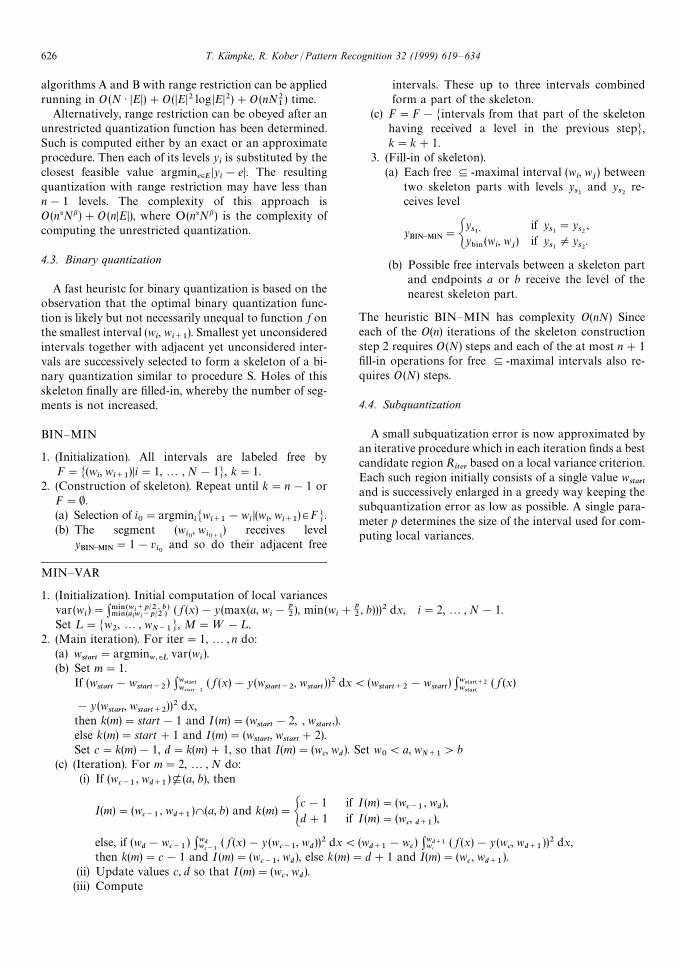
BIN—MIN

1. (Initialization). All intervals are labeled free byF"M(w

i, w

i`1)Di"1,2 , N!1N, k"1.

2. (Construction of skeleton). Repeat until k"n!1 orF"0.(a) Selection of i

0"argmin

iMw

i`1!w

iD(w

i, w

i`1)3FN.

(b) The segment (wi0, w

i0`1) receives level

yBIN~MIN

"1!vi0

and so do their adjacent free

intervals. These up to three intervals combinedform a part of the skeleton.

(c) F"F!Mintervals from that part of the skeletonhaving received a level in the previous stepN,k"k#1.

3. (Fill-in of skeleton).(a) Each free --maximal interval (w

i, w

j) between

two skeleton parts with levels ys1

and ys2

re-ceives level

yBIN~MIN

"Gys1,

if ys1"y

s2,

y"*/

(wi, w

j) if y

s1Oy

s2.

(b) Possible free intervals between a skeleton partand endpoints a or b receive the level of thenearest skeleton part.

The heuristic BIN—MIN has complexity O(nN) Sinceeach of the O(n) iterations of the skeleton constructionstep 2 requires O(N) steps and each of the at most n#1fill-in operations for free --maximal intervals also re-quires O(N) steps.

4.4. Subquantization

A small subquatization error is now approximated byan iterative procedure which in each iteration finds a bestcandidate region R

iterbased on a local variance criterion.

Each such region initially consists of a single value wstart

and is successively enlarged in a greedy way keeping thesubquantization error as low as possible. A single para-meter p determines the size of the interval used for com-puting local variances.

MIN—VAR

1. (Initialization). Initial computation of local variancesvar(w

i)":.*/(wi`p@2, b )

.*/(aiwi~p@2 )( f (x)!y(max(a, w

i!p

2), min(w

i#p

2, b)))2 dx, i"2,2 , N!1.

Set ¸"Mw2,2 , w

N~1N, M"¼!¸.

2. (Main iteration). For iter"1,2 , n do:(a) w

start"argmin

w,|Lvar(w

i).

(b) Set m"1.If (w

start!w

start~2) :w45!35

w45!35~2( f (x)!y (w

start~2, w

start))2 dx((w

start`2!w

start) :w45!35`2

w45!35( f (x)

!y (wstart

, wstart`2

))2 dx,then k(m)"start!1 and I (m)"(w

start!2, , w

start,).

else k(m)"start#1 and I(m)"(wstart

, wstart

#2).Set c"k(m)!1, d"k(m)#1, so that I(m)"(w

c, w

d). Set w

0(a, w

N`1'b

(c) (Iteration). For m"2,2 , N do:(i) If (w

c~1, w

d`1)¶(a, b), then

I(m)"(wc~1

, wd`1

)W(a, b) and k(m)"Gc!1 if I(m)"(w

c~1, w

d),

d#1 if I(m)"(wc,d`1

),

else, if (wd!w

c~1) :wd

wc~1( f (x)!y (w

c~1, w

d))2 dx((w

d`1!w

c) :wd`1

wc( f (x)!y (w

c, w

d`1))2 dx,

then k(m)"c!1 and I(m)"(wc~1

, wd), else k (m)"d#1 and I(m)"(w

c, w

d`1).

(ii) Update values c, d so that I (m)"(wc, w

d).

(iii) Compute


Fig. 3. Computation of s2,I

(thin lines) for the function f (N"55, thick lines) using MIN VAR. The parameter for the calculation of thelocal variance is set to p"5.

g (k(m))":wdwc

( f (x)!y (wc, w

d))2 dx

:ba( f (x)!y (a, b))2 dx

#1!m

N.

(d) Search for the first local minima of g()) left liter

and right riter

from xstart

to result in Riter

"(liter

, riter

).(e) Guarantee intervals R

iterto be disjunct: w

liter"max(w

liter, w

low`1with w

low"supMw

iDw

i3M and

wi(w

startN and w

riter"min(w

riter, w

up~1) with w

up"infMw

iDw

i3M and w

i'w

startN

(f ) Set ¸"¸!Mwliter

,2 , writer

N, M"M#Mwliter

,2, writer

N.

Procedure MIN—VAR runs in O (nN) time. Its effect isshown in Fig. 3.

A conceptually simpler algorithm than MIN—VAR isalso of an extension type. The largest level segments fromf serve as germs which are extended in a greedy manneruntil no further reduction of the subquantization error ispossible.

Ex1. (Initialization). The n longest level segments of f are

selected for R1,2 ,R

n. R"MR

1,2 , R

nN and

F"M(wi, w

i`1)Di"1,2 ,N!1N!R.

2. (Iteration). For i"1,2, n do:While R

ihas an adjacent level segment (w

k, w

k`1)

3F with E f!sn,R{

E#j(a, b)!R@ )(E f!sn,R

E#

j((a, b)!R), where R @"MR1,2 ,R

i~1, R

iX(w

k,

wk`1

), Ri`1

,2, RnN:

(a) Ri"R

iX(w

k, w

k`1),

(b) F"F!M(wk, w

k`1)N,

in case of two candidates (wk, w

k`1) the one with

smaller subquantization error is selected.

The complexity of Ex is O(nN). Interestingly, thiscomplexity is determined by the O(nN) complexity ofstep 1, while step 2 is only of complexity O(N) since atmost N-n extensions of intervals are possible overall.Computations and comparisons of subquantizationerrors in step 2 can be organized as in the exactprocedure Subquant.


Fig. 4. Upper image: f (x) (N"15, thick lines) and s (x) (thin lines) with an n computed using the criterion f(z). Lower image: f(z) with theoptimal value of n

0"7 indicated by the vertical line.

5. Segmentation issues

Determining the ‘‘correct’’ number of quantization seg-ments of a given signal is a difficult and rather unclearmatter. However, some criteria are proposed here, forother heuristics see [11].

One criterion suggesting the number of level segmentsis based on convex envelopes. Let l(x) be defined bylinearly interpolating the quantization error E f!s0

nE for

x3[2, N]. Function l is decreasing. By its lower convexenvelope l

l(x):"supMc (x)D c is convex and c(x))l(x)

∀x3[2, N]N a reasonable value for n is given by

n0" min

x|*2, N+Ml@

l(x)Dl@

l(x)*!

E f!s02E

N!2and

ll(x)"l(x)N;

there l@l(x)"l@

l(x#) for x3[2, N ) and l@

l(x)"l@

l(N!) for

x"N. The value n0

is the smallest such that the negativeslope of l

lreaches at least the average or secant slope

between l (2) and l (N )"0 and such that llsupports l.

Another criterion explicitely expresses the desire toobtain a small quantization error using a small number

of levels. The value for n is given by the first minimum ofthe function f (z), z"3,2 , N!1 starting at z"3 with

f(z)"E f!s0

zE

E f!s03E#A

z!1

N!2B2.

The first term of f decreases monotonically starting witha value of 1 at z"3. The second term of f increasesmonotonically reaching a value of 1 at z"N!1. Theeffect of this criterion is shown in Fig. 4. A third criterionis based on presumably salient frequency components.Let F ( ju)":b

af (x) e~+ux dx denote the Fourier trans-

formation of the step function f (x). Step functions areconsidered to have salient frequency componentsif u

.!9"argmaxu|(0, u

)*') )EFI (ju)E'2n/(b!a) with

FI denoting the Fourier transform of fI (x) andfI (x)"f (x)!y(a, b). A sufficiently large value of u

highmay be calculated using

:uhigh

0EFI ( ju)E du

:ba( f (x)!y(a, b))2 dx

'0.99.

The definition of a step function f (x) with sailent fre-quency components corresponds in the time domain to


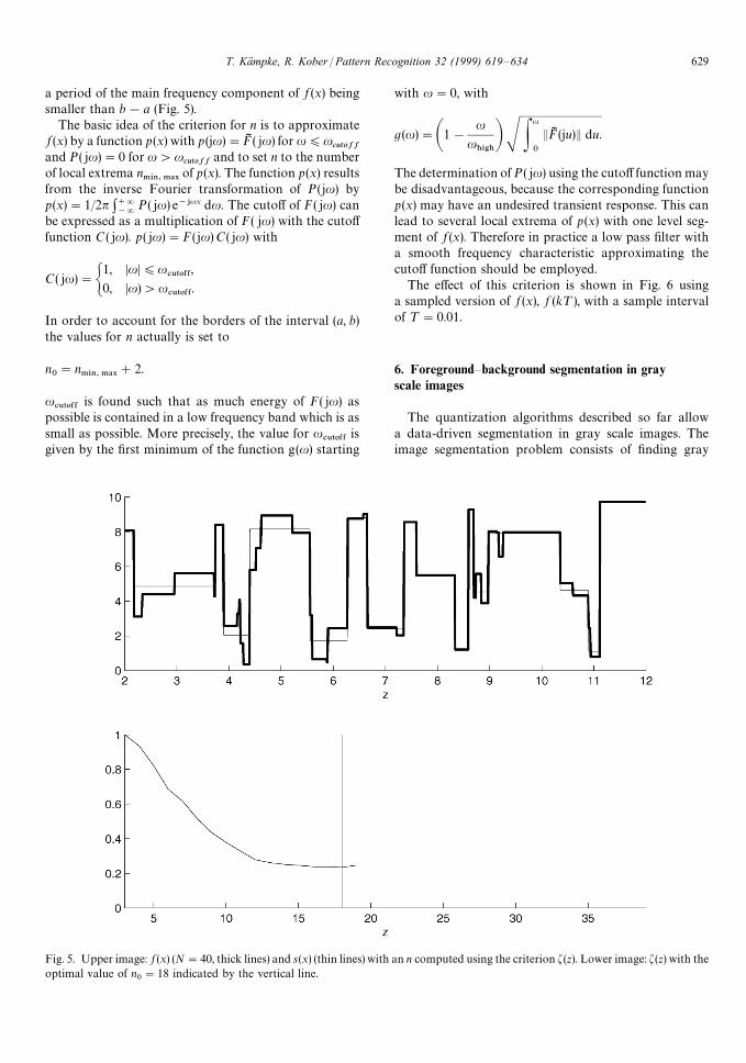
Fig. 5. Upper image: f (x) (N"40, thick lines) and s (x) (thin lines) with an n computed using the criterion f(z). Lower image: f(z) with theoptimal value of n

0"18 indicated by the vertical line.

a period of the main frequency component of f (x) beingsmaller than b!a (Fig. 5).

The basic idea of the criterion for n is to approximatef (x) by a function p (x) with p (ju)"FI ( ju) for u)u

cutoffand P( ju)"0 for u'u

cutoffand to set n to the number

of local extrema n.*/,.!9

of p(x). The function p(x) resultsfrom the inverse Fourier transformation of P(ju) byp(x)"1/2n :`=

~=P ( ju) e~+ux du. The cutoff of F( ju) can

be expressed as a multiplication of F( ju) with the cutofffunction C( ju). p ( ju)"F( ju) C( ju) with

C( ju)"G1, DuD)u

#650&&,

0, Du)'u#650&&

.

In order to account for the borders of the interval (a, b)the values for n actually is set to

n0"n

.*/,.!9#2.

u#650&&

is found such that as much energy of F( ju) aspossible is contained in a low frequency band which is assmall as possible. More precisely, the value for u

#650&&is

given by the first minimum of the function g(u) starting

with u"0, with

g(u)"A1!u

u)*')B S P

u

0

EFI (ju)E du.

The determination of P ( ju) using the cutoff function maybe disadvantageous, because the corresponding functionp(x) may have an undesired transient response. This canlead to several local extrema of p (x) with one level seg-ment of f (x). Therefore in practice a low pass filter witha smooth frequency characteristic approximating thecutoff function should be employed.

The effect of this criterion is shown in Fig. 6 usinga sampled version of f (x), f (k¹), with a sample intervalof ¹"0.01.

6. Foreground—background segmentation in grayscale images

The quantization algorithms described so far allowa data-driven segmentation in gray scale images. Theimage segmentation problem consists of finding gray


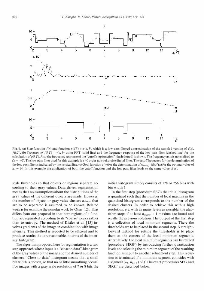
Fig. 6. (a) Step function f (x) and function p(k¹)#y(a, b), which is a low pass filtered approximation of the sampled version of f (x),f (k¹). (b) Spectrum of f (k¹)!y(a, b) using FFT (solid line) and the frequency response of the low pass filter (dashed line) for thecalculation of p (k¹). Also the frequency response of the ‘‘cutoff step function’’ (dash dotted) is shown. The frequency axis is normalized to)" w¹. The low pass filter used for this example is a 40 order non-rekursive digital filter. The cutoff frequency for the determination ofthe low pass filter is indicated by the vertical line. (c) Goal function g(w) for the determination of w

cutoff. (d) s0(x) for the optimal value of

n0"14. In this example the application of both the cutoff function and the low pass filter leads to the same value of n0.

scale thresholds so that objects or regions separate ac-cording to their gray values. Data driven segmentationmeans that no assumptions about the distributions of thegray values of the different objects are made. However,the number of objects or gray value clusters n

cluster

thatare to be separated is assumed to be known. Relatedwork is for example the popular work by Otsu [12]. Thatdiffers from our proposal in that here regions of a func-tion are separated according to its ‘‘coarse’’ peaks ratherthan to entropy. The method of Kittler et al. [13] in-volves gradients of the image in combination with imageintensity. This method is reported to be efficient and toproduce results that are reasonable in terms of the inten-sity histogram.

The algorithm proposed here for segmentation is a twostep approach whose input is a ‘‘close to data’’-histogramof the gray values of the image and the desired number ofclusters. ‘‘Close to data’’-histogram means that a smallbin width is chosen, so that no or little smoothing occurs.For images with a gray scale resolution of 7 or 8 bits the

initial histogram simply consists of 128 or 256 bins withbin width 1.

In the first step (procedure SEG) the initial histogramis quantized such that the number of local maxima in thequantized histogram corresponds to the number of thedesired clusters. In order to achieve this with a highresolution, e.g. with as many levels as possible, the algo-rithm stops if at least n

cluster#1 maxima are found and

recalls the previous solution. The output of the first stepis a collection of local minimum segments. There thethresholds are to be placed in the second step. A straight-forward method for setting the thresholds is to placethem at the centers of the local minimum segments.Alternatively, the local minimum segments can be refined(procedure SEGF) by introducing further quantizationlevels and selecting the minimum segment of the resultingfunction as input to another refinement step. This recur-sion is terminated if a minimum segment coincides witha segment (w

k, w

k`1) of f. The exact procedures SEG and

SEGF are described below.


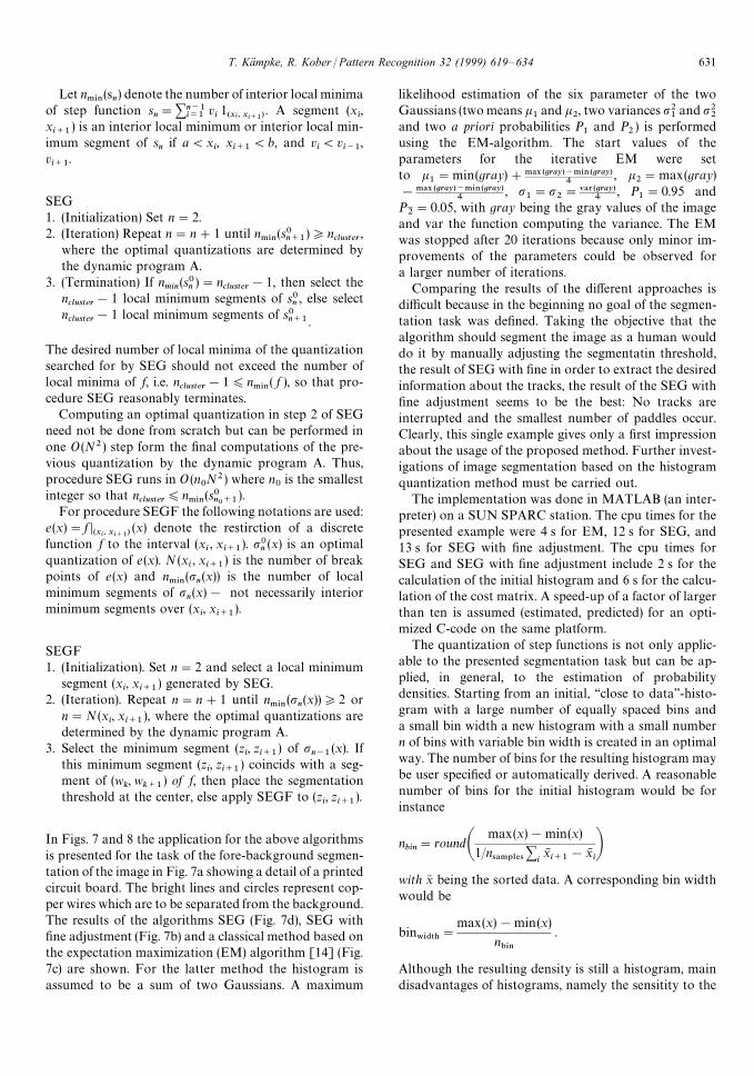
Let n.*/

(sn) denote the number of interior local minima

of step function sn"+n~1

i/1vi1(xi, xi`1)

. A segment (xi,

xi`1

) is an interior local minimum or interior local min-imum segment of s

nif a(x

i, x

i`1(b, and v

i(v

i~1,

vi`1

.

SEG1. (Initialization) Set n"2.2. (Iteration) Repeat n"n#1 until n

.*/(s0n`1

)*ncluster

,where the optimal quantizations are determined bythe dynamic program A.

3. (Termination) If nmin

(s0n)"n

cluster!1, then select the

ncluster

!1 local minimum segments of s0n, else select

ncluster

!1 local minimum segments of s0n`1 .

The desired number of local minima of the quantizationsearched for by SEG should not exceed the number oflocal minima of f, i.e. n

cluster!1)n

.*/( f ), so that pro-

cedure SEG reasonably terminates.Computing an optimal quantization in step 2 of SEG

need not be done from scratch but can be performed inone O(N2 ) step form the final computations of the pre-vious quantization by the dynamic program A. Thus,procedure SEG runs in O (n

0N2 ) where n

0is the smallest

integer so that ncluster

)n.*/

(s0n0`1

).For procedure SEGF the following notations are used:

e(x)"f D(xi, xi`1)

(x) denote the restirction of a discretefunction f to the interval (x

i, x

i`1). p0

n(x) is an optimal

quantization of e (x). N (xi, x

i`1) is the number of break

points of e(x) and n.*/

(pn(x)) is the number of local

minimum segments of pn(x)! not necessarily interior

minimum segments over (xi, x

i`1).

SEGF1. (Initialization). Set n"2 and select a local minimum

segment (xi, x

i`1) generated by SEG.

2. (Iteration). Repeat n"n#1 until n.*/

(pn(x))*2 or

n"N(xi, x

i`1), where the optimal quantizations are

determined by the dynamic program A.3. Select the minimum segment (z

i, z

i`1) of p

n~1(x). If

this minimum segment (zi, z

i`1) coincids with a seg-

ment of (wk, w

k`1) of f, then place the segmentation

threshold at the center, else apply SEGF to (zi, z

i`1).

In Figs. 7 and 8 the application for the above algorithmsis presented for the task of the fore-background segmen-tation of the image in Fig. 7a showing a detail of a printedcircuit board. The bright lines and circles represent cop-per wires which are to be separated from the background.The results of the algorithms SEG (Fig. 7d), SEG withfine adjustment (Fig. 7b) and a classical method based onthe expectation maximization (EM) algorithm [14] (Fig.7c) are shown. For the latter method the histogram isassumed to be a sum of two Gaussians. A maximum

likelihood estimation of the six parameter of the twoGaussians (two means k

1and k

2, two variances p2

1and p2

2and two a priori probabilities P

1and P

2) is performed

using the EM-algorithm. The start values of theparameters for the iterative EM were setto k

1"min(gray)#.!9 (gray)~.*/ (gray)

4, k

2"max(gray)

!.!9 (gray)~.*/(gray)4

, p1"p

2"7!3 (gray)

4, P

1"0.95 and

P2"0.05, with gray being the gray values of the image

and var the function computing the variance. The EMwas stopped after 20 iterations because only minor im-provements of the parameters could be observed fora larger number of iterations.

Comparing the results of the different approaches isdifficult because in the beginning no goal of the segmen-tation task was defined. Taking the objective that thealgorithm should segment the image as a human woulddo it by manually adjusting the segmentatin threshold,the result of SEG with fine in order to extract the desiredinformation about the tracks, the result of the SEG withfine adjustment seems to be the best: No tracks areinterrupted and the smallest number of paddles occur.Clearly, this single example gives only a first impressionabout the usage of the proposed method. Further invest-igations of image segmentation based on the histogramquantization method must be carried out.

The implementation was done in MATLAB (an inter-preter) on a SUN SPARC station. The cpu times for thepresented example were 4 s for EM, 12 s for SEG, and13 s for SEG with fine adjustment. The cpu times forSEG and SEG with fine adjustment include 2 s for thecalculation of the initial histogram and 6 s for the calcu-lation of the cost matrix. A speed-up of a factor of largerthan ten is assumed (estimated, predicted) for an opti-mized C-code on the same platform.

The quantization of step functions is not only applic-able to the presented segmentation task but can be ap-plied, in general, to the estimation of probabilitydensities. Starting from an initial, ‘‘close to data’’-histo-gram with a large number of equally spaced bins anda small bin width a new histogram with a small numbern of bins with variable bin width is created in an optimalway. The number of bins for the resulting histogram maybe user specified or automatically derived. A reasonablenumber of bins for the initial histogram would be forinstance

nbin"roundA

max(x)!min(x)

1/n4!.1-%4

+ixNi`1

!xNiB

with x6 being the sorted data. A corresponding bin widthwould be

bin8*$5)

"

max(x)!min(x)

n"*/

.

Although the resulting density is still a histogram, maindisadvantages of histograms, namely the sensitity to the


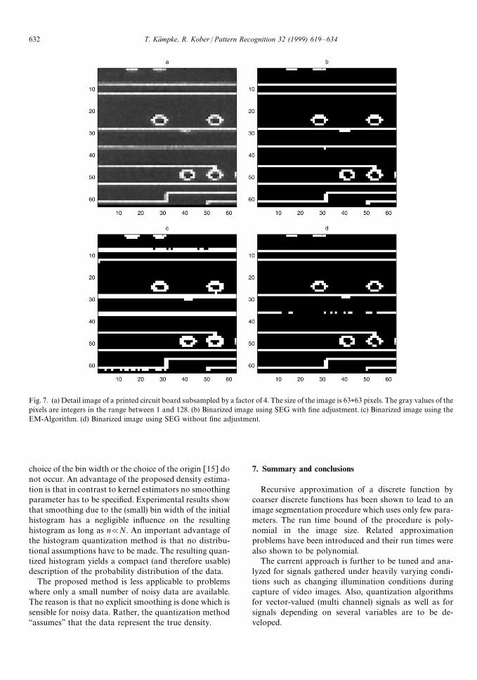
Fig. 7. (a) Detail image of a printed circuit board subsampled by a factor of 4. The size of the image is 63*63 pixels. The gray values of thepixels are integers in the range between 1 and 128. (b) Binarized image using SEG with fine adjustment. (c) Binarized image using theEM-Algorithm. (d) Binarized image using SEG without fine adjustment.

choice of the bin width or the choice of the origin [15] donot occur. An advantage of the proposed density estima-tion is that in contrast to kernel estimators no smoothingparameter has to be specified. Experimental results showthat smoothing due to the (small) bin width of the initialhistogram has a negligible influence on the resultinghistogram as long as n@N. An important advantage ofthe histogram quantization method is that no distribu-tional assumptions have to be made. The resulting quan-tized histogram yields a compact (and therefore usable)description of the probability distribution of the data.

The proposed method is less applicable to problemswhere only a small number of noisy data are available.The reason is that no explicit smoothing is done which issensible for noisy data. Rather, the quantization method‘‘assumes’’ that the data represent the true density.

7. Summary and conclusions

Recursive approximation of a discrete function bycoarser discrete functions has been shown to lead to animage segmentation procedure which uses only few para-meters. The run time bound of the procedure is poly-nomial in the image size. Related approximationproblems have been introduced and their run times werealso shown to be polynomial.

The current approach is further to be tuned and ana-lyzed for signals gathered under heavily varying condi-tions such as changing illumination conditions duringcapture of video images. Also, quantization algorithmsfor vector-valued (multi channel) signals as well as forsignals depending on several variables are to be de-veloped.


Fig. 8. (a) Histogram of the gray values of the image in Fig. 7 using 128 bins. (b) Detailed view of the lower part of Fig 7a. (c) Quantizedhistogram (thin line) of the histogram in (a) using procedure SEG with fine adjustment and the probability distribution (thick line)resulting from the EM-algorithm assuming a sum of two gaussians. The corresponding thresholds for the segmentation of foregroundand background are indicated by the thick (EM) and thin (SEG with fine adjustment) vertical line. (d) Detailed view of the lower part ofFig. 7c.

References

[1] A. Gersho, R.M. Gray, Vector quantization and SignalCompression. Kluver, Boston, 1992.

[2] K. Donner, Hierarchical approximation for pattern recog-nition, Proc. Applications of Artificial Intelligence (AAAI1991), pp. 213—226. Prague, 1991.

[3] W. Koller, Segmentierung und Diagnose von Gefaben mitAtlasunterstutzung. VDI-Verlag, Dusseldorf, 1995.

[4] P. Bock, R. Klinnert, R. Kober, R.M. Rovner, H. Schmidt,Gray-Scale ALIAS, IEEE Trans. Knowledge Data Eng.4(2) (1992) 109—122.

[5] H. Schmidt, Histogrammbasierte klassifikation von sen-sordaten, Dissertation, University of Ulm, 1993.

[6] D. Mumford, Pattern theory: a unifying perspective, Pre-print, Harvard University, 1993.

[7] D. Mumford, J. Shah, Optimal approximations bypiecewise smooth functions and associated vari-ational problems, Commun. Pure Appl. Math 42 (1989)577—685.

[8] A. Blake, A. Zisserman, Visual reconstruction. MIT Press,Cambridge MA, 1979.

[9] D.J. Berndt, J. Clifford, Finding patterns in time series:a dynamic programming approach, in: U.M. Fayyad et al.(Eds), Advances in Knowledge Discovery and Data Min-ing, pp. 229—248. MIT Press, Menlo Park, 1996.

[10] T. Kampke, Optimal and near optimal quantizaton ofintegrable functions, submitted.

[11] T. Kampke, Efficient quantization algorithms for discretefunctions, in progress.

[12] N. Otsu, A threshold selection method from gray-scalehistograms , IEEE Trans Systems, Man, and Cybernetics8 (1978) 62—66.

[13] J. Kittler, J. Illingworth, J. Foglein, K. Paler, An automaticthresholding algorithm and its performance. Proc. 7th Int.conf. on pattern recognition, Montreal, (1984) pp. 213—226.

[14] R. Duda, P. Hart, Pattern Classification and Scene Analy-sis. Wiley New York 1973.

[15] B.W. Silverman, Density Estimation, Chapman & Hall,London, New York, 1986.


About the Author—THOMAS KA® MPKE holds a diploma and a Ph.D. in mathematics from the University of Aachen, Germany. Hehas been visiting the University of California at Berkeley by a grant from the Humboldt foundation. He is working in various areasrelated to applied mathematics such as discrete and stochastic optimization, planning and control of autonomous mobile systems, signalanalysis, processing of uncertain information. and bioinformatics.

About the Author—RUDOLF KOBER received his diploma in biology in 1983 and his doctoral degree in physiology and electronics in1988 from the University of Tubingen, Germany. From 1988 to 1990 he was a post-doctoral scientist at the Institute of Communicationsin Erlangen. From 1990 to 1997 he was a scientist with the FAW, working in areas of neural networks, pattern recognition, signal andimage processing and control theory. Since 1997 he has been with the company Orto MAQUET, working in the area of computer-assisted orthopedic surgery.


Documents

Discrete signal quantization