Embed Size (px)
Citation preview
M I C H A E L B R A U N
D I S C R E T E S T R U C T U R E S

Preface
The manuscript serves as an introduction to the theory of dis-crete structures. The focus lies on algorithms for the enumerativegeneration, construction, and classification of discrete structures.A corresponding lecture was given during the summer term in2014 at the University of Applied Sciences, Darmstadt, Germany.
Munich, November 25, 2014 Michael Braun

Contents
Introduction 7
Subsets and Gray codes 11
k-Subsets and the revolving door algorithm 19
Subspaces of a vector space over a finite field 25
Permutations and the Johnson-Trotter algorithm 33
Cycle type of permutations and integer partitions 39
Groups and permutations 45
Group actions 55
Similar group actions 63
6 michael braun
Orbit Evaluation 69
Counting orbits 75
Bibliography 81
Introduction
Discrete structures arise by iterated conjunction, combinationor selection of elementary objects as lists, sets and subsets, orpermutations. In this manuscript we investigate some basicconcepts and combinatorial algorithms for discrete structures.
There are many cases where different objects of the sametype actually represent the identical structure. For instance, ifwe want to represent k-element subsets of the finite set V =
0, . . . , n− 1 by lists of length k containing the elements of thesubset we get different representations for the same subset. Forexample, if S = 1, 3, 4 is a subset of V = 0, 1, 2, 3, 4, we getthe six lists
[1, 3, 4], [1, 4, 3], [3, 1, 4], [3, 4, 1], [4, 1, 3], [4, 3, 1]
representing the same subset S. In this case it is appropriate tocollect all these vectors in one single equivalence class representingone particular subset. It is obvious to see that all vectors withinthe same equivalence class can be obtained from an initial vectorby permuting the coordinates in all possible ways.
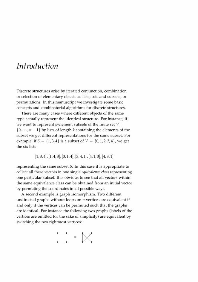
A second example is graph isomorphism. Two differentundirected graphs without loops on n vertices are equivalent ifand only if the vertices can be permuted such that the graphsare identical. For instance the following two graphs (labels of thevertices are omitted for the sake of simplicity) are equivalent byswitching the two rightmost vertices:
8 michael braun
In general the goal is to classify a set of objects of a particulartype according to the given equivalence relation. In most casesthe equivalence relation “'” arises by permuting components ofthe objects. This leads to the concept of group actions.
Explicit listing of all objects of a particular type is a primarygoal in combinatorics. If possible it is desirable to design algo-rithms to generate all objects in a certain order and algorithms tocompute the position of an object within this order or to generatethe object from its position number. For rudimentary structuresas subsets, permutations, partitions, or graphs such algorithmsare known. In other cases where objects are partitioned intoclasses of equivalent objects we want to generate representativesof all equivalence classes. In general such algorithms involvegroup theoretic aspects.
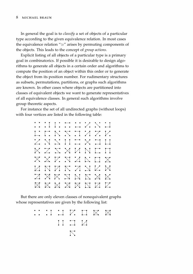
For instance the set of all undirected graphs (without loops)with four vertices are listed in the following table:
But there are only eleven classes of nonequivalent graphswhose representatives are given by the following list:
discrete structures 9
The third goal is to count the number of objects of a particulartype. Of course by explicit generation of all objects we also gettheir number. But for many discrete structures where parametersget too large generating all objects is computationally infeasible.In this case it is often easier to determine the number of objectsdirectly without generating them since an explicit countingformula is known. For instance, the number of k-element subsetsof an n-element set is given by the Binomial coefficient (n
k) =n!
k!(n−k)! or the number of all subsets of an n-element set is 2n.The number of undirected graphs without loops with n verticesis given by 2(
n2). But in cases where we want to count the number
of equivalence classes of objects of a particular type the situationbecomes more complicated and involves group theory again.
For instance the number of equivalence classes of undirectedgraphs without loops on n vertices can be computed with the aidof the Cauchy-Frobenius formula
∑a an
2|〈πa〉\\(n2)|
∏ni=1 iai ai!
.
Note that in the case of four vertices n = 4 we get eleven classesof nonequivalent graphs.
Another important aim in combinatorics is to construct anobject with specified properties, for instance a linear [n, k]qcode with a certain minimum distance. Generating all objectsuntil the desired one is obtained is not efficient in most cases.Many interesting construction problems can be formulated asinteger optimization problem belonging to the class of NP-hardproblems. Therefore no efficient algorithms are known for theconstruction of the corresponding combinatorial objects. Inthis case we restrict the search area by prescribing additionalsymmetry properties the objects to be constructed must fulfill.Here the symmetry properties arise by automorphism groupsinduced by a predefined group action.
The manuscript is organized as follows:In the first chapters we introduce some rudimentary struc-
tures we are going to use for further investigations in the latterchapters. We describe representations and algorithms for thegeneration of sets, subsets, permutations, partitions, and subspaces.
10 michael braun
Afterwards we consider groups and the action of groups ondifferent sets of discrete structures. With the aid of such groupactions we are able to partition the set of objects into classes ofisomorphic or equivalent objects. We define automorphism groups ofobjects which play a major role to construct all elements of oneisomorphism class. Finally, we present an algorithm to generaterepresentatives and automorphism groups of equivalence classes.
In the last part of the manuscript we investigate some appli-cations for which the proposed concept of group actions andisomorphism can be used to classify and construct certain objects.We consider the classification of graphs by isomorphism, theenumeration of isomers of chemical molecules, and the construc-tion of linear codes, designs, and random network codes withprescribed groups of automorphisms.
Subsets and Gray codes
In this chapter we consider subsets of finite sets, their repre-sentation and basic operations. Furthermore, we introduce theconcept of enumerative generation of discrete structures in gen-eral. Finally, we describe the binary reflected Gray code for theenumerative generation of all subsets of a finite set.
Since all finite sets of the same cardinality n ∈ N can be bijec-tively mapped onto each other we can restrict our investigationsto the canonic n-element set of the form V = 0, . . . , n− 1.
In the following we denote by S ⊆ V a subset of V. Thisnotation also includes that S and V can be equal. To indicate thatS is a proper subset of V we use the symbol S ⊂ V or S ( V.Subsets S of cardinality 0 ≤ k ≤ n, abbreviated by |S| = k, arecalled k-element subsets or simply k-subsets.
In order to represent subsets S ⊆ V we can use different datastructures.
The obvious possibility is to represent a k-subset S as aninteger vector [x0, . . . , xk−1] containing the sorted elementsof S = x0, . . . , xk−1, i.e. x0 < . . . < xk−1. Set operationsas membership testing of elements x ∈ S, and insertion ordeletion involve a linear and binary search on the vector havingcomplexity O(k) and O(log k), respectively.
A second representation on which we focus within this chap-ter is the characteristic vector of a subset. A subset S ⊆ V isidentified with a binary vector a = a0 . . . an−1 of length n whereai = 1 if i ∈ S and ai = 0 if otherwise. We have to mention thatthis way of representing subsets is only appropriate for practi-cal implementations if the finite set V is sufficiently small andbinary vectors of length n can be stored and accessed easily—for
12 michael braun
instance in an unsigned w-bit integer word or in an array ofdn/we unsigned integers if n > w.
Now we investigate the basic operations on subsets using thecharacteristic vector. For this purpose let a be the characteristicvector of the subset S and b the corresponding vector of thesubset T. All vector operations are immediate from the definitionof the set operations.
Membership test. To check whether an element i ∈ V is con-tained in S we verify if ai is 1 or 0.
Insertion. To insert an element i ∈ V into S we set ai := 1.Deletion. To erase an element i ∈ V from S we set ai := 0.Cardinality. To determine the cardinality of S we compute the
Hamming weight
wt(a) := |i | 0 ≤ i < n, ai 6= 0|
of a which is the number of nonzero positions in a.Complement. The setwise complement of S defined by the
subsetS := V \ S := x ∈ V | x 6∈ S
can be computed by bitwise complementing the elements ofa which means that are zero becomes one and vice versa. Thecorresponding vector is denoted by
¬a := ¬a0 . . .¬an−1.
Intersection. The intersection
S ∩ T := x ∈ V | x ∈ S and x ∈ T
can be computed by the bitwise boolean and-operator “∧” de-fined by
a ∧ b := a0 ∧ b0 . . . an−1 ∧ bn−1.
Union. The vector operation on the union
S ∪ T := x ∈ V | x ∈ S or x ∈ T
immediately arises from the bitwise boolean or-operator “∨” andyields
a ∨ b := a0 ∨ b0 . . . an−1 ∨ bn−1.
discrete structures 13
Note that membership testing, insertion, and deletion can beperformed in O(1) and computing the cardinality, complement,intersection and union has linear complexity O(n).
Next, we discuss the generation of all subsets of an n-elementset. Using the notion of characteristic vectors this issue is equiv-alent to the generation of all binary vectors of length n. A quitenatural approach to solve this task is the use of the reflectedbinary number representation of the numbers 0, 1, 2, . . . , 2n − 1which generates all possible 2n binary vectors of length n in alexicographic order: If a0 . . . an−1 denotes the binary vector thecorresponding integer—which is called (lexicographic) rank—isdefined to be
n−1
∑i=0
ai2i.
It gives the position within the ordering of all possible binaryvectors. Finally, we get a one-to-one-correspondence betweensubsets, binary vectors, and integers as we can see in the follow-ing example.
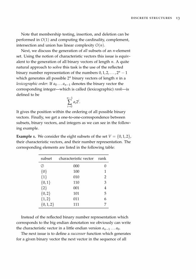
Example 1. We consider the eight subsets of the set V = 0, 1, 2,their characteristic vectors, and their number representation. Thecorresponding elements are listed in the following table:
subset characteristic vector rank
∅ 000 00 100 11 010 20, 1 110 32 001 40, 2 101 51, 2 011 60, 1, 2 111 7
Instead of the reflected binary number representation whichcorresponds to the big endian denotation we obviously can writethe characteristic vector in a little endian version an−1 . . . a0.
The next issue is to define a successor function which generatesfor a given binary vector the next vector in the sequence of all
14 michael braun
binary vectors with respect to the given ordering. In the case ofthe mentioned lexicographic ordering given by the binary integerrepresentation the successor b = b0 . . . bn−1 of a = a0 . . . an−1
satisfiesn−1
∑i=0
bi2i =
(n−1
∑i=0
ai2i
)+ 1
(except for the final binary vector a = 11 . . . 1).Note that the concept of (enumerative) generation of all objects
of a certain type can be formulated in a more general notion.Let X be a finite set of objects of a certain type. The rank
function determines the position of an object x ∈ X and is givenby a bijective mapping
rank : X → 0, . . . , |X| − 1.
Conversely, the corresponding inverse function is called unrank
unrank : 0, . . . , |X| − 1 → X.
By definition both functions satisfy the property
rank(x) = i ⇐⇒ unrank(i) = x
for all objects x ∈ X and integers 0 ≤ i < |X|.The successor function, abbreviated by
succ : X → X ∪ ⊥,
generates for a given object x ∈ X the consecutive object y ∈ Xwith respect to the ordering induced by the rank function. To bemore precise we get the equivalence
y = succ(x) ⇐⇒ rank(y) = rank(x) + 1.
In fact there is one exceptional case: If x ∈ X denotes the lastelement within the ordering, i.e. rank(x) = |X| − 1, its successoris defined to be the undefined value “⊥”. Finally we obtain
succ(x) :=
unrank(rank(x) + 1) if rank(x) < |X| − 1,
⊥ otherwise.
discrete structures 15
In some cases the undefined value can be avoid if the successorfunction implements a cyclic shift on the set X. In this casethe successor of the last element is again the first object in theordering. In this case the successor satisfies
succ(x) := unrank(rank(x) + 1 mod |X|).
In an analogous way we can also define the predecessor func-tion
pred : X → X ∪ ⊥
realizing
pred(x) :=
unrank(rank(x)− 1) if rank(x) > 0,
⊥ otherwise.
The benefits of the concept of enumerative generation using rank,unrank, successor or predecessor functions are immediate.
As the term enumerative generation says the obvious appli-cation is the generation of all elements in the induced orderingwithout storing all of them. For this purpose we can iterate overall integers 0 ≤ i < |X| and compute unrank(i) to get all objects.
A second possibility is to take the successor function anditerate x(i) := succ(x(i−1)) with x(0) := unrank(0) until all objectsof X are visited.
Another potential application is the generation of objectsuniformly at random with probability 1/|X|. Using an unbiasedrandom number generator we just have to pick a random integeri between 0 and |X| − 1 and compute unrank(i).
If we can measure the distance between the objects of X by ametric function d : X× X → R, i.e. d(x, y) means the distance be-tween x and y, a natural goal is to find a sequence of x(0), x(1), . . .of all objects of X such that the distance d(x(i−1), x(i)) betweenthe element x(i−1) and its successor x(i)is minimal. A sequencesatisfying this property for all of its elements has a minimalchange ordering.
Example 2. The sequence
Γ3 = 000, 001, 011, 010, 110, 111, 101, 100
16 michael braun
traverses all binary vectors of length 3 in a minimal changeordering with respect to the Hamming distance which counts thenumber of positions in which two vectors differ. In the givensequence all pairs of consecutive vectors differ in exactly oneposition—they have Hamming distance 1.
In the following we define the recurrence for a sequence Γn ofall binary vectors of length n in minimal change ordering tracingback to Gray1. Due to its construction it is also called binary 1 F. Gray. Pulse Code
Communication. U.S. Patent2,632,058, March 1953 (filedNov. 1947)
reflected Gray code.First we consider some rudimentary constructions of se-
quences. If a = a0 . . . an−1 denotes a binary vector of length n wedefine the extension
a0 := a0 . . . an−10
a1 := a0 . . . an−11
of a by one coordinate.Furthermore if Γ = a(0), . . . , a(`−1) and Ω = b(0), . . . , b(m−1)
denote sequences of binary vectors of length n we define threeoperations.
Concatenation.
Γ, Ω := a(0), . . . , a(`−1), b(0), . . . , b(m−1)
Reflection.ΓR := a(`−1), . . . , a(0)
Augmentation.
Γ0 := a(0)0, . . . , a(`−1)0
Γ1 := a(0)1, . . . , a(`−1)1
The following lemma can immediately be deduced from thesebasic constructions.
Lemma 1. If Γ denotes a minimal change sequence of binary vectors oflength n then Γ0, ΓR1 is a minimal change sequence of binary vectors oflength n + 1.
Using this construction in a recursive way and starting withthe right initial sequence we get a minimal change sequence onall binary vectors of a given length.
discrete structures 17
Theorem 1. Let n be a positive integer. The recurrence
Γ1 := 0, 1
Γi := Γi−10, ΓRi−11, i ≥ 1
defines a minimal change sequence Γn on the set of all binary vectors oflength n.
Proof. By induction and due to Lemma 1 the sequence Γn isobviously a minimal change sequence. Furthermore since |Γi| =2|Γi−1| with |Γ1| = 2 we get |Γn| = 2n.
Example 3. We consider the first 4 sequences:
Γ1 = 0, 1
Γ2 = 0|0, 1|0, 1|1, 0|1Γ3 = 00|0, 10|0, 11|0, 01|0, 01|1, 11|1, 10|1, 00|1Γ4 = 000|0, 100|0, 110|0, 010|0, 011|0, 111|0, 101|0, 001|0,
001|1, 101|1, 111|1, 011|1, 010|1, 110|1, 100|1, 000|1
Problem 1. Develop and implement a rank, unrank, and succes-sor function for the sequence Γn.
Problem 2. Develop and implement a minimal change algorithmto traverse all vectors of length n with entries 0, 1, . . . , q− 1 fora positive integer q. Develop and implement a rank, unrank, andsuccessor function for the corresponding sequence.
The binary reflected Gray code was named by Frank Graywho invented Γn for the pulse code modulation in 1951, amethod for analog transmission of digital signals2. 2 F. Gray. Pulse Code
Communication. U.S. Patent2,632,058, March 1953 (filedNov. 1947)
In fact, Gray codes were used before by Stibitz3 in 1943.
3 G. Stibitz. Binary Counter.U.S. Patent 2,307,868, 1943
Knuth mentioned in4 that Γ5 was used in a telegraph machine
4 D. E. Knuth. The Art ofComputer Programming, Vol-ume 4, Fascicle 2: GeneratingAll Tuples and Permutations.Addison-Wesley, 2005
by Émile Baudot in 1878.
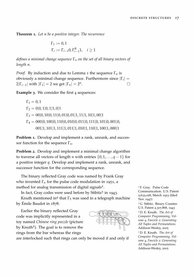
Earlier the binary reflected Graycode was implicitly represented in atoy named Chinese ring puzzle (pictureby Knuth5). The goal is to remove the
5 D. E. Knuth. The Art ofComputer Programming, Vol-ume 4, Fascicle 2: GeneratingAll Tuples and Permutations.Addison-Wesley, 2005
rings from the bar whereas the ringsare interlocked such that rings can only be moved if and only if
18 michael braun
the ring to its right is on the bar and all rings to the right of thatare off the bar. The current state of the puzzle can be representedas a binary vector where rings on the bar correspond to 1 andrings off the bar are written as 0.
Note that permuting the vector coordinates in each vector ofthe Gray code turns the code into another minimal change code.A comprehensive overview on the different possible Gray codescan be found in Knuth’s book6. 6 D. E. Knuth. The Art of
Computer Programming, Vol-ume 4, Fascicle 2: GeneratingAll Tuples and Permutations.Addison-Wesley, 2005
k-Subsets and the revolving door algorithm
A well-known counting formula to determine the number ofpossibilities to choose k elements from an n-element set yieldsthe Binomial coefficient(
nk
)=
n!k!(n− k)!
.
The goal of this chapter is to generate all these possibilities. Tobe more precise if V = 0, . . . , n− 1 again denotes the canonicn-element set we use(
Vk
):= S ⊆ V | |S| = k
for the set of k-subsets of V and we want to generate all of itselements.
The enumerative generation algorithm we are going to presentis based on the constructive proof of the recurrence formula ofthe Binomial coefficient(
nk
)=
(n− 1
k
)+
(n− 1k− 1
)
with initial values (n0
)=
(nn
)= 1
which is called the Pascal’s identity. Arranging these values in atriangle yields the well-known Pascal’s triangle:
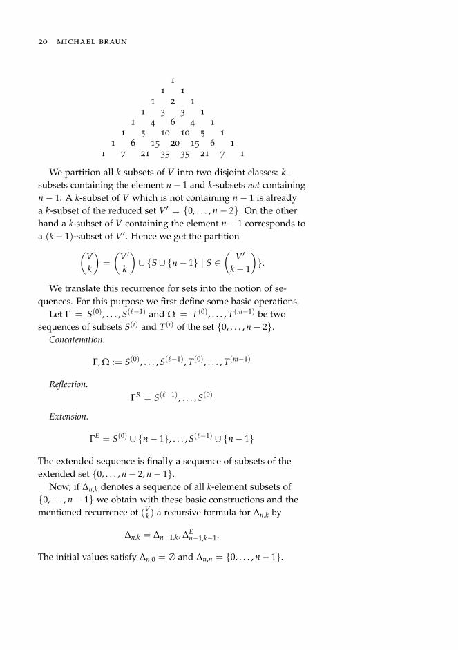
20 michael braun
1
1 1
1 2 1
1 3 3 1
1 4 6 4 1
1 5 10 10 5 1
1 6 15 20 15 6 1
1 7 21 35 35 21 7 1
We partition all k-subsets of V into two disjoint classes: k-subsets containing the element n− 1 and k-subsets not containingn− 1. A k-subset of V which is not containing n− 1 is alreadya k-subset of the reduced set V′ = 0, . . . , n− 2. On the otherhand a k-subset of V containing the element n− 1 corresponds toa (k− 1)-subset of V′. Hence we get the partition(
Vk
)=
(V′
k
)∪ S ∪ n− 1 | S ∈
(V′
k− 1
).
We translate this recurrence for sets into the notion of se-quences. For this purpose we first define some basic operations.
Let Γ = S(0), . . . , S(`−1) and Ω = T(0), . . . , T(m−1) be twosequences of subsets S(i) and T(i) of the set 0, . . . , n− 2.
Concatenation.
Γ, Ω := S(0), . . . , S(`−1), T(0), . . . , T(m−1)
Reflection.ΓR = S(`−1), . . . , S(0)
Extension.
ΓE = S(0) ∪ n− 1, . . . , S(`−1) ∪ n− 1
The extended sequence is finally a sequence of subsets of theextended set 0, . . . , n− 2, n− 1.
Now, if ∆n,k denotes a sequence of all k-element subsets of0, . . . , n− 1 we obtain with these basic constructions and thementioned recurrence of (V
k ) a recursive formula for ∆n,k by
∆n,k = ∆n−1,k, ∆En−1,k−1.
The initial values satisfy ∆n,0 = ∅ and ∆n,n = 0, . . . , n− 1.
discrete structures 21
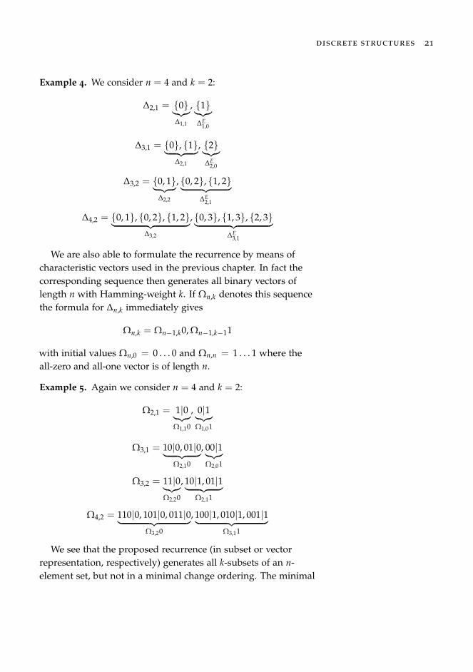
Example 4. We consider n = 4 and k = 2:
∆2,1 = 0︸︷︷︸∆1,1
, 1︸︷︷︸∆E
1,0
∆3,1 = 0, 1︸ ︷︷ ︸∆2,1
, 2︸︷︷︸∆E
2,0
∆3,2 = 0, 1︸ ︷︷ ︸∆2,2
, 0, 2, 1, 2︸ ︷︷ ︸∆E
2,1
∆4,2 = 0, 1, 0, 2, 1, 2︸ ︷︷ ︸∆3,2
, 0, 3, 1, 3, 2, 3︸ ︷︷ ︸∆E
3,1
We are also able to formulate the recurrence by means ofcharacteristic vectors used in the previous chapter. In fact thecorresponding sequence then generates all binary vectors oflength n with Hamming-weight k. If Ωn,k denotes this sequencethe formula for ∆n,k immediately gives
Ωn,k = Ωn−1,k0, Ωn−1,k−11
with initial values Ωn,0 = 0 . . . 0 and Ωn,n = 1 . . . 1 where theall-zero and all-one vector is of length n.
Example 5. Again we consider n = 4 and k = 2:
Ω2,1 = 1|0︸︷︷︸Ω1,10
, 0|1︸︷︷︸Ω1,01
Ω3,1 = 10|0, 01|0︸ ︷︷ ︸Ω2,10
, 00|1︸︷︷︸Ω2,01
Ω3,2 = 11|0︸︷︷︸Ω2,20
, 10|1, 01|1︸ ︷︷ ︸Ω2,11
Ω4,2 = 110|0, 101|0, 011|0︸ ︷︷ ︸Ω3,20
, 100|1, 010|1, 001|1︸ ︷︷ ︸Ω3,11
We see that the proposed recurrence (in subset or vectorrepresentation, respectively) generates all k-subsets of an n-element set, but not in a minimal change ordering. The minimal
22 michael braun
change property here means that we get from one subset to itsconsecutive subset by exchanging just one element.
The following theorem gives a recurrence formula for a mini-mal change sequence of k-subsets.
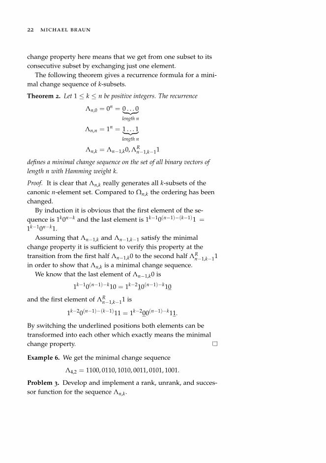
Theorem 2. Let 1 ≤ k ≤ n be positive integers. The recurrence
Λn,0 = 0n = 0 . . . 0︸ ︷︷ ︸length n
Λn,n = 1n = 1 . . . 1︸ ︷︷ ︸length n
Λn,k = Λn−1,k0, ΛRn−1,k−11
defines a minimal change sequence on the set of all binary vectors oflength n with Hamming weight k.
Proof. It is clear that Λn,k really generates all k-subsets of thecanonic n-element set. Compared to Ωn,k the ordering has beenchanged.
By induction it is obvious that the first element of the se-quence is 1k0n−k and the last element is 1k−10(n−1)−(k−1)1 =
1k−10n−k1.Assuming that Λn−1,k and Λn−1,k−1 satisfy the minimal
change property it is sufficient to verify this property at thetransition from the first half Λn−1,k0 to the second half ΛR
n−1,k−11in order to show that Λn,k is a minimal change sequence.
We know that the last element of Λn−1,k0 is
1k−10(n−1)−k10 = 1k−210(n−1)−k10
and the first element of ΛRn−1,k−11 is
1k−20(n−1)−(k−1)11 = 1k−200(n−1)−k11.
By switching the underlined positions both elements can betransformed into each other which exactly means the minimalchange property.
Example 6. We get the minimal change sequence
Λ4,2 = 1100, 0110, 1010, 0011, 0101, 1001.
Problem 3. Develop and implement a rank, unrank, and succes-sor function for the sequence Λn,k.
discrete structures 23
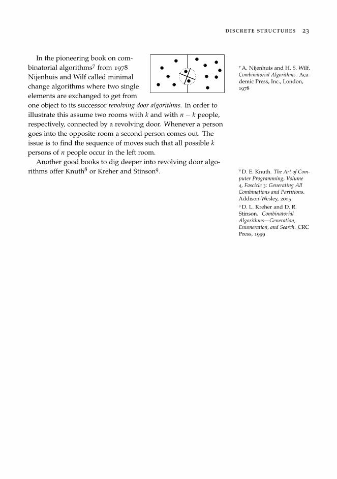
In the pioneering book on com-binatorial algorithms7 from 1978
7 A. Nijenhuis and H. S. Wilf.Combinatorial Algorithms. Aca-demic Press, Inc., London,1978
Nijenhuis and Wilf called minimalchange algorithms where two singleelements are exchanged to get fromone object to its successor revolving door algorithms. In order toillustrate this assume two rooms with k and with n− k people,respectively, connected by a revolving door. Whenever a persongoes into the opposite room a second person comes out. Theissue is to find the sequence of moves such that all possible kpersons of n people occur in the left room.
Another good books to dig deeper into revolving door algo-rithms offer Knuth8 or Kreher and Stinson9. 8 D. E. Knuth. The Art of Com-
puter Programming, Volume4, Fascicle 3: Generating AllCombinations and Partitions.Addison-Wesley, 2005
9 D. L. Kreher and D. R.Stinson. CombinatorialAlgorithms—Generation,Enumeration, and Search. CRCPress, 1999

Subspaces of a vector space over a finite field
In this chapter we generate all k-dimensional subspaces of ann-dimensional vector space over a finite field. For this purposewe recall some basic facts of linear algebra.
In the following let Fq denote a finite field with q elements. Ingeneral a field F is a set together with addition and multiplica-tion rules such that F is a commutative additive group, F \ 0 acommutative multiplicative group, and such that the distributivelaw a(b + c) = ab + ac is satisfied for all a, b, c ∈ F. A finitefield Fq of order q exists if and only if q is a prime power. If q isa prime the corresponding field is given by Fq = 0, 1, . . . , q− 1and addition as well as multiplication is performed modulo q.
The set Fnq denotes the set of all column vectors
x =
x0...
xn−1
= [x0, . . . , xn−1]t
with entries in Fq. It forms a vector space with respect to thevector addition
x0...
xn−1
+
y0...
yn−1
:=
x0 + y0
...xn−1 + yn−1
for x, y ∈ Fn
q and scalar multiplication
λ
x0...
xn−1
:=
λx0
...λxn−1
26 michael braun
for λ ∈ Fq and x ∈ Fnq .
A linear combination of vectors b0, . . . , bk−1 ∈ Fnq is an ex-
pression of the form ∑k−1i=0 λibi = λ0b0 + . . . + λk−1bk−1 ∈ Fn
qwhere λi ∈ Fq are field elements for all 0 ≤ i < k. The vectorsb0, . . . , bk−1 are called linearly independent if and only if the zerovector can be linearly combined only trivialy by zero coefficients,i.e. 0 = ∑k−1
i=0 λibi implies λi = 0 for all 0 ≤ i < k.If b0, . . . , bk−1 ∈ Fn
q denotes a set of linearly independentvectors the set of all possible linear combinations defines a k-dimensional subspace S of Fq:
S = 〈b0, . . . , bk−1〉 = k−1
∑i=0
λibi | λi ∈ Fq.
Obviously, we get |S| = qk since we have k different coefficientswhere each of them can be any element of Fq. The set of vectorsb0, . . . , bk−1 ∈ Fn
q is called a basis of S.Hence each k-dimensional subspace of Fn
q can be representedby an n× k matrix over Fq where its columns denote a basis of thesubspace. By Gaussian elimination which is a clever sequence ofelementary transformations of the columns, namely
• swapping two columns,
• multiplying each element of a column by a nonzero fieldelement,
• adding the multiple of a column to a second column,
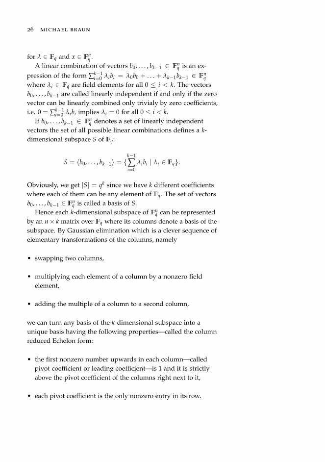
we can turn any basis of the k-dimensional subspace into aunique basis having the following properties—called the columnreduced Echelon form:
• the first nonzero number upwards in each column—calledpivot coefficient or leading coefficient—is 1 and it is strictlyabove the pivot coefficient of the columns right next to it,
• each pivot coefficient is the only nonzero entry in its row.
discrete structures 27
∗ ∗ ∗...
......
∗ ∗ ∗1 0 0
∗ ∗...
...∗ ∗1 0
∗. . .
...∗1
0...0
In our definition we omit all-zero columns which are usually
allowed in Echelon forms. Furthermore in classical textbooksand research articles instead of the column representation rowreduced Echelon forms are considered. In this manuscript thecolumn version has been chosen to be consistent with groupactions of matrix groups on subspaces from the left—which wewill use later.
Problem 4. Implement an algorithm to compute the columnreduced Echelon form of an n× k matrix over a field Fq with qprime.
If Gk(n, q) denotes the set of all k-dimensional subspacesof Fn
q , called the Grassmannian, the goal of this chapter is togenerate all elements of Gk(n, q).
Lemma 2. The number of k-dimensional subspaces of Fnq is given by
the expression[nk
]q
:=(qn − 1)(qn−1 − 1) · · · (qn−k+1 − 1)
(qk − 1)(qk−1 − 1) · · · (q− 1)
which is called the Gaussian coefficient or q-binomial coefficients.
Proof. In order to determine the number of k-dimensional sub-spaces of Fn
q we count the number of possibilities to k linearly
28 michael braun
independent vectors in Fnq . For the first columns we have take all
nonzero vectors of length n, i.e. qn − 1. For the second columnwe take all vectors which are linearly independent from the firstcolumn, i.e. qn − q. In general the ith vector must be linearlyindependent from the preceding i− 1 vectors which means thatwe have qn − qi possibilities to chose the ith column. Finally thenumber of possibilities to chose k linearly independent vectors ofFn
q is
(qn − 1)(qn − q)(qn − q2) · · · (qn − qk−1).
Analogously, the term
(qk − 1)(qk − q)(qk − q2) · · · (qk − qk−1)
yields the number of bases for the same k-dimensional subspaceof V. The quotient of both expressions is the required number ofk-dimensional subspaces of V. After simplifying we obtain thestated ratio for Gk(n, q).
Corollary 1. The Gaussian coefficient satisfies[nn
]q=
[n0
]q= 1.
In the following we want generate all possible column re-duced Echelon forms of size n× k with entries in Fq, which finallyrepresent all k-dimensional subspaces of Fn
q . For this purpose letΓn,k,q denote the set of all column reduced Echelon forms of sizen× k over Fq.
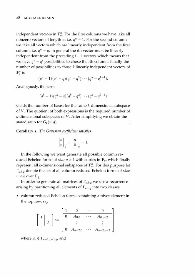
In order to generate all matrices of Γn,k,q we use a recurrencearising by partitioning all elements of Γn,k,q into two classes:
• column reduced Echelon forms containing a pivot element inthe top row, say
[1
A
]:=
1 0 · · · 00 A0,0 · · · A0,k−2...
......
0 An−2,0 · · · An−2,k−2
where A ∈ Γn−1,k−1,q, and
discrete structures 29
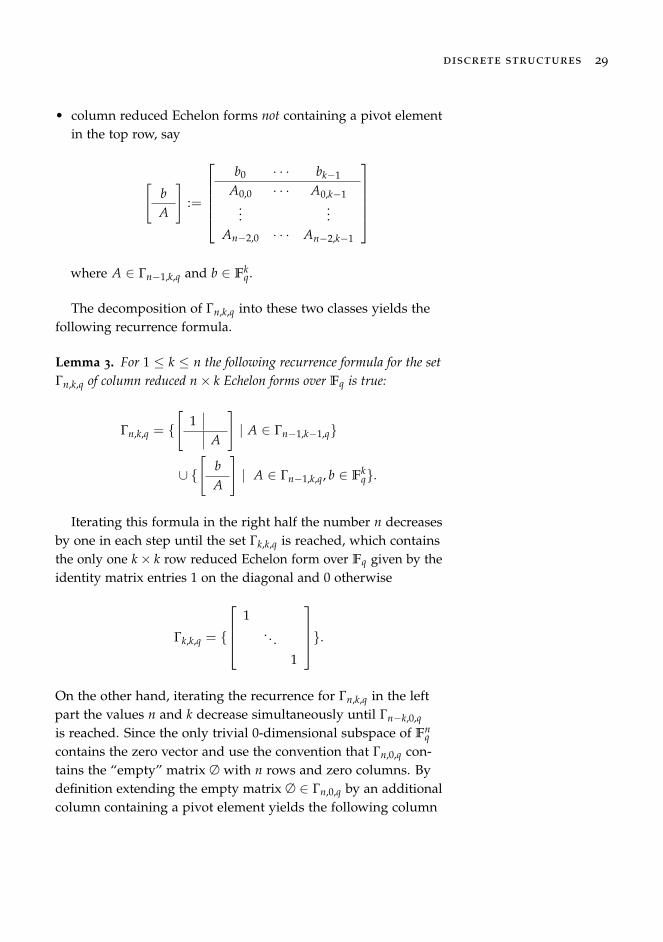
• column reduced Echelon forms not containing a pivot elementin the top row, say
[bA
]:=
b0 · · · bk−1
A0,0 · · · A0,k−1...
...An−2,0 · · · An−2,k−1
where A ∈ Γn−1,k,q and b ∈ Fk
q.
The decomposition of Γn,k,q into these two classes yields thefollowing recurrence formula.
Lemma 3. For 1 ≤ k ≤ n the following recurrence formula for the setΓn,k,q of column reduced n× k Echelon forms over Fq is true:
Γn,k,q = [
1A
]| A ∈ Γn−1,k−1,q
∪ [
bA
]| A ∈ Γn−1,k,q, b ∈ Fk
q.
Iterating this formula in the right half the number n decreasesby one in each step until the set Γk,k,q is reached, which containsthe only one k× k row reduced Echelon form over Fq given by theidentity matrix entries 1 on the diagonal and 0 otherwise
Γk,k,q =
1
. . .1
.On the other hand, iterating the recurrence for Γn,k,q in the leftpart the values n and k decrease simultaneously until Γn−k,0,q
is reached. Since the only trivial 0-dimensional subspace of Fnq
contains the zero vector and use the convention that Γn,0,q con-tains the “empty” matrix ∅ with n rows and zero columns. Bydefinition extending the empty matrix ∅ ∈ Γn,0,q by an additionalcolumn containing a pivot element yields the following column
30 michael braun
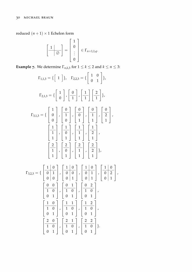
reduced (n + 1)× 1 Echelon form
[1
∅
]=
10...0
∈ Γn+1,1,q.
Example 7. We determine Γn,k,3 for 1 ≤ k ≤ 2 and k ≤ n ≤ 3:
Γ1,1,3 = [
1], Γ2,2,3 =
[1 00 1
],
Γ2,1,3 = [
10
],
[01
],
[11
] [21
],
Γ3,1,3 =
100
,
010
,
001
,
011
,
021
,
111
,
101
,
111
,
121
,
211
,
201
,
211
,
221
,
Γ3,2,3 =
1 00 10 0
,
1 00 00 1
,
1 00 10 1
,
1 00 20 1
,
0 01 00 1
,
0 11 00 1
,
0 21 00 1
,
1 01 00 1
,
1 11 00 1
,
1 21 00 1
,
2 01 00 1
,
2 11 00 1
,
2 21 00 1
.
discrete structures 31
Problem 5. Write a program to generate all elements of Γn,k,q us-ing the given recurrence. Implement rank, unrank and successor.
Problem 6. Design a minimal change sequence for Γn,k,q whereminimal change means that two consecutive n× k Echelon formsdiffer by exactly one coordinate.
As an immediate consequence from the recurrence for Γn,k,q
where each matrix of Γn−1,k,q is combined with each vector of Fkq
we get the recursive formula for the Gaussian coefficient.
Corollary 2. For 1 ≤ k ≤ n the Gaussian coefficient satisfies therecurrence [
nk
]q=
[n− 1k− 1
]q+ qk
[n− 1
k
]q.

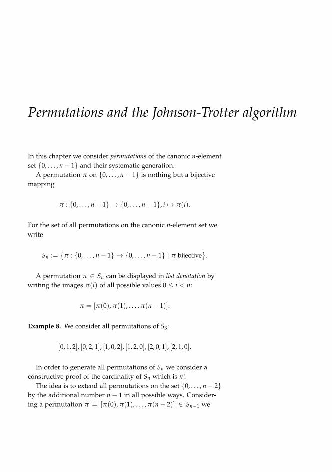
Permutations and the Johnson-Trotter algorithm
In this chapter we consider permutations of the canonic n-elementset 0, . . . , n− 1 and their systematic generation.
A permutation π on 0, . . . , n− 1 is nothing but a bijectivemapping
π : 0, . . . , n− 1 → 0, . . . , n− 1, i 7→ π(i).
For the set of all permutations on the canonic n-element set wewrite
Sn :=
π : 0, . . . , n− 1 → 0, . . . , n− 1 | π bijective
.
A permutation π ∈ Sn can be displayed in list denotation bywriting the images π(i) of all possible values 0 ≤ i < n:
π = [π(0), π(1), . . . , π(n− 1)].
Example 8. We consider all permutations of S3:
[0, 1, 2], [0, 2, 1], [1, 0, 2], [1, 2, 0], [2, 0, 1], [2, 1, 0].
In order to generate all permutations of Sn we consider aconstructive proof of the cardinality of Sn which is n!.
The idea is to extend all permutations on the set 0, . . . , n− 2by the additional number n− 1 in all possible ways. Consider-ing a permutation π = [π(0), π(1), . . . , π(n− 2)] ∈ Sn−1 we
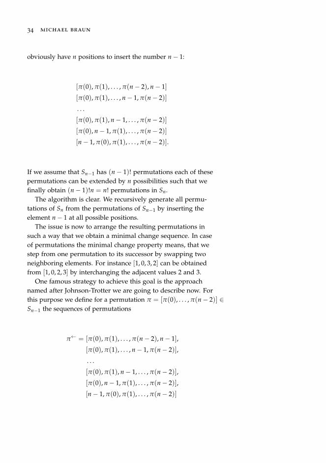
34 michael braun
obviously have n positions to insert the number n− 1:
[π(0), π(1), . . . , π(n− 2), n− 1]
[π(0), π(1), . . . , n− 1, π(n− 2)]
. . .
[π(0), π(1), n− 1, . . . , π(n− 2)]
[π(0), n− 1, π(1), . . . , π(n− 2)]
[n− 1, π(0), π(1), . . . , π(n− 2)].
If we assume that Sn−1 has (n− 1)! permutations each of thesepermutations can be extended by n possibilities such that wefinally obtain (n− 1)!n = n! permutations in Sn.
The algorithm is clear. We recursively generate all permu-tations of Sn from the permutations of Sn−1 by inserting theelement n− 1 at all possible positions.
The issue is now to arrange the resulting permutations insuch a way that we obtain a minimal change sequence. In caseof permutations the minimal change property means, that westep from one permutation to its successor by swapping twoneighboring elements. For instance [1, 0, 3, 2] can be obtainedfrom [1, 0, 2, 3] by interchanging the adjacent values 2 and 3.
One famous strategy to achieve this goal is the approachnamed after Johnson-Trotter we are going to describe now. Forthis purpose we define for a permutation π = [π(0), . . . , π(n− 2)] ∈Sn−1 the sequences of permutations
π← = [π(0), π(1), . . . , π(n− 2), n− 1],
[π(0), π(1), . . . , n− 1, π(n− 2)],
. . .
[π(0), π(1), n− 1, . . . , π(n− 2)],
[π(0), n− 1, π(1), . . . , π(n− 2)],
[n− 1, π(0), π(1), . . . , π(n− 2)]
discrete structures 35
and
π→ = [n− 1, π(0), π(1), . . . , π(n− 2)],
[π(0), n− 1, π(1), . . . , π(n− 2)],
[π(0), π(1), n− 1, . . . , π(n− 2)],
. . .
[π(0), π(1), . . . , n− 1, π(n− 2)],
[π(0), π(1), . . . , π(n− 2), n− 1].
Note that if π, ρ ∈ Sn−1 denote two permutations whose listdenotation can be transformed into each other by interchangingtwo adjacent elements the corresponding sequence Σ = π←, ρ→
consisting of 2n permutations of Sn has the minimal changeproperty. With this observation we get the following recurrenceon Sn.
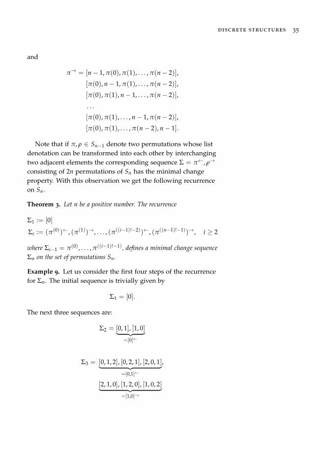
Theorem 3. Let n be a positive number. The recurrence
Σ1 := [0]
Σi := (π(0))←, (π(1))→, . . . , (π((i−1)!−2))←, (π((n−1)!−1))→, i ≥ 2
where Σi−1 = π(0), . . . , π((i−1)!−1), defines a minimal change sequenceΣn on the set of permutations Sn.
Example 9. Let us consider the first four steps of the recurrencefor Σn. The initial sequence is trivially given by
Σ1 = [0].
The next three sequences are:
Σ2 = [0, 1], [1, 0]︸ ︷︷ ︸=[0]←
Σ3 = [0, 1, 2], [0, 2, 1], [2, 0, 1]︸ ︷︷ ︸=[0,1]←
,
[2, 1, 0], [1, 2, 0], [1, 0, 2]︸ ︷︷ ︸=[1,0]→
36 michael braun
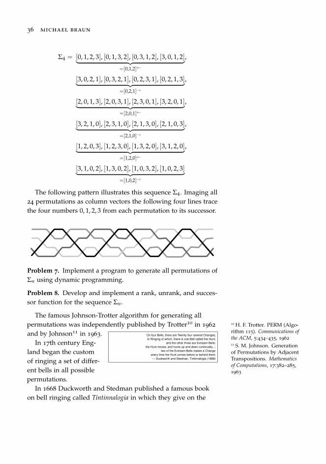
Σ4 = [0, 1, 2, 3], [0, 1, 3, 2], [0, 3, 1, 2], [3, 0, 1, 2]︸ ︷︷ ︸=[0,1,2]←
,
[3, 0, 2, 1], [0, 3, 2, 1], [0, 2, 3, 1], [0, 2, 1, 3]︸ ︷︷ ︸=[0,2,1]→
,
[2, 0, 1, 3], [2, 0, 3, 1], [2, 3, 0, 1], [3, 2, 0, 1]︸ ︷︷ ︸=[2,0,1]←
,
[3, 2, 1, 0], [2, 3, 1, 0], [2, 1, 3, 0], [2, 1, 0, 3]︸ ︷︷ ︸=[2,1,0]→
,
[1, 2, 0, 3], [1, 2, 3, 0], [1, 3, 2, 0], [3, 1, 2, 0]︸ ︷︷ ︸=[1,2,0]←
,
[3, 1, 0, 2], [1, 3, 0, 2], [1, 0, 3, 2], [1, 0, 2, 3]︸ ︷︷ ︸=[1,0,2]→
The following pattern illustrates this sequence Σ4. Imaging all24 permutations as column vectors the following four lines tracethe four numbers 0, 1, 2, 3 from each permutation to its successor.
Problem 7. Implement a program to generate all permutations ofΣn using dynamic programming.
Problem 8. Develop and implement a rank, unrank, and succes-sor function for the sequence Σn.
The famous Johnson-Trotter algorithm for generating allpermutations was independently published by Trotter10 in 1962
10 H. F. Trotter. PERM (Algo-rithm 115). Communications ofthe ACM, 5:434–435, 1962
and by Johnson11 in 1963.11 S. M. Johnson. Generationof Permutations by AdjacentTranspositions. Mathematicsof Computations, 17:382–285,1963
On four Bells, there are Twenty four several Changes,In Ringing of which, there is one Bell called the Hunt,
and the other three are Extream Bells;the Hunt moves, and hunts up and down continually...;
two of the Extream Bells makes a Changeevery time the Hunt comes before or behind them.— Duckworth and Stedman, Tintinnalogia (1668)
In 17th century Eng-land began the customof ringing a set of differ-ent bells in all possiblepermutations.
In 1668 Duckworth and Stedman published a famous bookon bell ringing called Tintinnalogia in which they give on the

discrete structures 37
first 60 pages a detailed description on the sequence Σn of allpermutations, which they simply call plain changes.

Cycle type of permutations and integer partitions
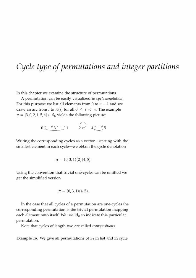
In this chapter we examine the structure of permutations.A permutation can be easily visualized in cycle denotation.
For this purpose we list all elements from 0 to n − 1 and wedraw an arc from i to π(i) for all 0 ≤ i < n. The exampleπ = [3, 0, 2, 1, 5, 4] ∈ S6 yields the following picture:
0 '' 3 '' 1jj 2 qq 4 '' 5gg
Writing the corresponding cycles as a vector—starting with thesmallest element in each cycle—we obtain the cycle denotation
π = (0, 3, 1)(2)(4, 5).
Using the convention that trivial one-cycles can be omitted weget the simplified version
π = (0, 3, 1)(4, 5).
In the case that all cycles of a permutation are one-cycles thecorresponding permutation is the trivial permutation mappingeach element onto itself. We use idn to indicate this particularpermutation.
Note that cycles of length two are called transpositions.
Example 10. We give all permutations of S3 in list and in cycle
40 michael braun
denotation:
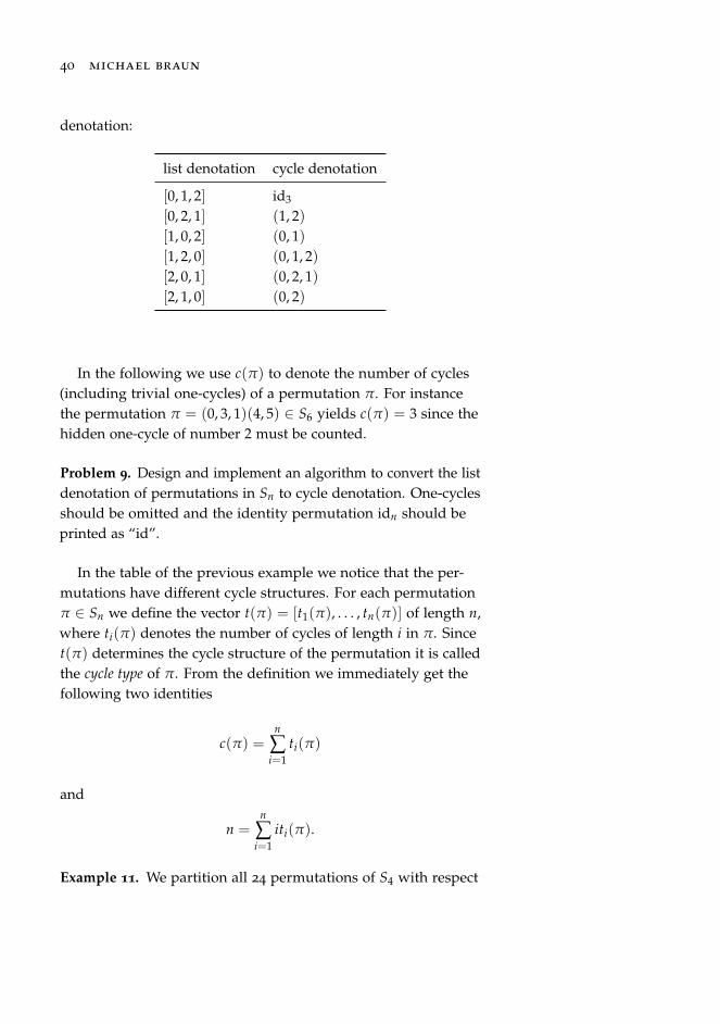
list denotation cycle denotation
[0, 1, 2] id3
[0, 2, 1] (1, 2)[1, 0, 2] (0, 1)[1, 2, 0] (0, 1, 2)[2, 0, 1] (0, 2, 1)[2, 1, 0] (0, 2)
In the following we use c(π) to denote the number of cycles(including trivial one-cycles) of a permutation π. For instancethe permutation π = (0, 3, 1)(4, 5) ∈ S6 yields c(π) = 3 since thehidden one-cycle of number 2 must be counted.
Problem 9. Design and implement an algorithm to convert the listdenotation of permutations in Sn to cycle denotation. One-cyclesshould be omitted and the identity permutation idn should beprinted as “id”.
In the table of the previous example we notice that the per-mutations have different cycle structures. For each permutationπ ∈ Sn we define the vector t(π) = [t1(π), . . . , tn(π)] of length n,where ti(π) denotes the number of cycles of length i in π. Sincet(π) determines the cycle structure of the permutation it is calledthe cycle type of π. From the definition we immediately get thefollowing two identities
c(π) =n
∑i=1
ti(π)
and
n =n
∑i=1
iti(π).
Example 11. We partition all 24 permutations of S4 with respect
discrete structures 41
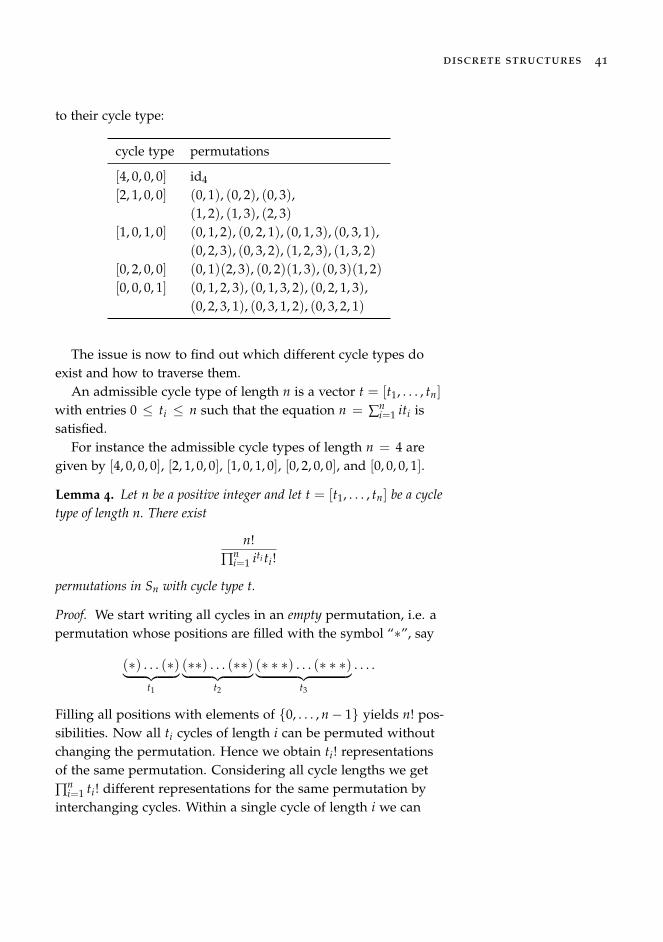
to their cycle type:
cycle type permutations
[4, 0, 0, 0] id4
[2, 1, 0, 0] (0, 1), (0, 2), (0, 3),(1, 2), (1, 3), (2, 3)
[1, 0, 1, 0] (0, 1, 2), (0, 2, 1), (0, 1, 3), (0, 3, 1),(0, 2, 3), (0, 3, 2), (1, 2, 3), (1, 3, 2)
[0, 2, 0, 0] (0, 1)(2, 3), (0, 2)(1, 3), (0, 3)(1, 2)[0, 0, 0, 1] (0, 1, 2, 3), (0, 1, 3, 2), (0, 2, 1, 3),
(0, 2, 3, 1), (0, 3, 1, 2), (0, 3, 2, 1)
The issue is now to find out which different cycle types doexist and how to traverse them.
An admissible cycle type of length n is a vector t = [t1, . . . , tn]
with entries 0 ≤ ti ≤ n such that the equation n = ∑ni=1 iti is
satisfied.For instance the admissible cycle types of length n = 4 are
given by [4, 0, 0, 0], [2, 1, 0, 0], [1, 0, 1, 0], [0, 2, 0, 0], and [0, 0, 0, 1].
Lemma 4. Let n be a positive integer and let t = [t1, . . . , tn] be a cycletype of length n. There exist
n!∏n
i=1 iti ti!
permutations in Sn with cycle type t.
Proof. We start writing all cycles in an empty permutation, i.e. apermutation whose positions are filled with the symbol “∗”, say
(∗) . . . (∗)︸ ︷︷ ︸t1
(∗∗) . . . (∗∗)︸ ︷︷ ︸t2
(∗ ∗ ∗) . . . (∗ ∗ ∗)︸ ︷︷ ︸t3
. . . .
Filling all positions with elements of 0, . . . , n− 1 yields n! pos-sibilities. Now all ti cycles of length i can be permuted withoutchanging the permutation. Hence we obtain ti! representationsof the same permutation. Considering all cycle lengths we get∏n
i=1 ti! different representations for the same permutation byinterchanging cycles. Within a single cycle of length i we can
42 michael braun
perform cyclic shifts without changing the permutation. Hencefor ti cycles of length i we get iti representations of the samepermutation. Again considering all cycle lengths we get ∏n
i=1 iti
versions of one permutation by shifting cycles. Altogether wehave ∏n
i=1 ti! ·∏i=1 iti = ∏ni=1 iti ti! different representations of the
same permutation. Dividing all possibilities n! by all differentrepresentations yields the required formula.
Problem 10. Design and implement an algorithm to generate allcycle types of length n.
In order to describe the cycle structure of permutations wecan also use an equivalent representation which is given by(integer) partitions. By writing the cycle lengths of a permutationin weakly decreasing order we get a partition.
More formally, a vector (p0, . . . , pm−1) with positive integerssatisfying p0 ≥ . . . ≥ pm−1 and n = ∑m−1
i=0 pi is called a partitionof n.
Obviously we can transform a cycle type t = [t1, . . . , tn] oflength n into a partition
ntn n− 1tn−1 . . . 1t1 = (n, . . . , n︸ ︷︷ ︸tn
, n− 1, . . . , n− 1︸ ︷︷ ︸tn−1
, . . . , 1, . . . , 1︸ ︷︷ ︸t1
)
and vice versa.
Example 12. The five cycle types [4, 0, 0, 0], [2, 1, 0, 0], [1, 0, 1, 0],[0, 2, 0, 0], [0, 0, 0, 1] of length 4 correspond to the five partitions(1, 1, 1, 1), (2, 1, 1), (3, 1), (2, 2), (4).
Problem 11. Describe an algorithm to transform a partition intothe corresponding cycle type.
Problem 12. Design and implement an algorithm to generate allpartitions of n.
There is a very famous formula to determine the number sn,k
of permutations of length n having exactly k cycles. The numbersn,k is called the Stirling number of the first kind and satisfies
sn,k = sn−1,k−1 + (n− 1)sn−1,k.
discrete structures 43
The proof is quite simple and somehow analogous to the proofof the Pascal’s identity for Binomial coefficients. A permutationπ of length n with k cycles arises either by a permutation of theset 0, . . . , n− 2 with k− 1 cycles by adding a further elementn− 1 in a one-cycle, or by a permutation of the set 0, . . . , n− 2with k cycles where the additional element n− 1 must be insertedin any of the k cycles. Since the order of the elements in thecycles must be respected the element n− 1 can be inserted in acycle after any of the n− 1 elements.
Example 13. We construct all s4,3 permutations of length 4 having3 cycles. There are s3,2 = 3 permutations on the set 0, 1, 2having 2 cycles (one-cycles are displayed!): (0)(1, 2), (0, 1)(2),(0, 2)(1). Insertion of an additional one-cycle with the element3 yields the permutations (0)(1, 2)(3), (0, 1)(2)(3), (0, 2)(1)(3).On the other hand there is exactly s3,3 = 1 permutation ofthe set 0, 1, 2 having three cycles, the identity permutationid3 = (0)(1)(2). Inserting the element 3 at all positions yields(0, 3)(1)(2), (0)(1, 3)(2), (0)(1)(2, 3), altogether six permutationsof length 4 with 3 cycles.
Problem 13. Design and implement a recurrence formula for theset of all permutations n with k cycles utilizing the recurrencesn,k = sn−1,k−1 + (n− 1)sn−1,k for its quantity.
The denotation Stirling number of the first kind suggeststhe existence of further Stirling numbers. Indeed there are theStirling numbers of the second kind Sn,k which count the numberof possibilities to decompose a set of n objects into k parts.
The Stirling numbers are named after the scottish mathe-matician James Stirling (1692-1770) and were published in hismanuscript Methodis Differentialis in 1730.

Groups and permutations
In this chapter we examine the structure of the set Sn of permu-tations. Permutations in Sn correspond to bijective mappingsof the set 0, . . . , n − 1. By the composition “” of mappingswe obtain a multiplication rule on the set of permutations Sn. Ifπ, ρ ∈ Sn denote two permutations we get a third permutationσ = πρ ∈ Sn by
σ(i) = (πρ)(i) := (π ρ)(i) = π(ρ(i))
for all 0 ≤ i < n.From the properties of the composition rule of mappings we
deduce that the multiplication of permutations is associative forall τ, π, ρ ∈ Sn:
τ(πρ) = (τπ)ρ.
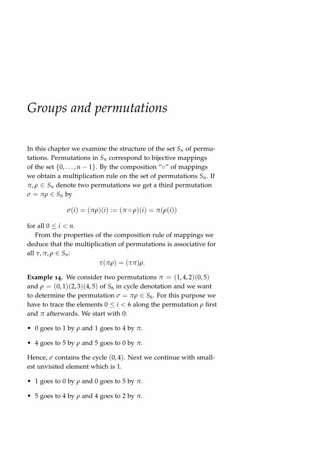
Example 14. We consider two permutations π = (1, 4, 2)(0, 5)and ρ = (0, 1)(2, 3)(4, 5) of S6 in cycle denotation and we wantto determine the permutation σ = πρ ∈ S6. For this purpose wehave to trace the elements 0 ≤ i < 6 along the permutation ρ firstand π afterwards. We start with 0:
• 0 goes to 1 by ρ and 1 goes to 4 by π.
• 4 goes to 5 by ρ and 5 goes to 0 by π.
Hence, σ contains the cycle (0, 4). Next we continue with small-est unvisited element which is 1.
• 1 goes to 0 by ρ and 0 goes to 5 by π.
• 5 goes to 4 by ρ and 4 goes to 2 by π.
46 michael braun
• 2 goes to 3 by ρ and 3 goes to 3 by π (a hidden one-cycle).
• 3 goes to 2 by ρ and 2 goes to 1 by π.
The cycle is finished, i.e. σ contains the cycle (1, 5, 2, 3). Finally,we obtain the permutation σ = πρ = (0, 4)(1, 5, 2, 3).
Note that the multiplication of permutations is not commuta-tive in general, i.e. it does not satisfy πρ = ρπ for all π, σ ∈ Sn.For instance the two permutations π, ρ in the previous exampleyield the product ρπ = (0, 4, 3, 2)(1, 5) which is different fromπρ = (0, 4)(1, 5, 2, 3).
A particular permutation contained in Sn is the identity map-ping idn, i.e. it consists of trivial one-cycles 1n = (0)(1) . . . (n− 1).Multiplication of any permutation π ∈ Sn with idn leaves thepermutation invariant:
π idn = idn π = π.
Another important property is the existence of inverse ele-ments. Since each permutation π ∈ Sn is a bijective mappingthere exists a corresponding mapping ρ ∈ Sn reverting the firstpermutation π:
ρ : π(i) 7→ i.
Composition of both yields the identity mapping ρπ = idn. Inthis case we also write
π−1 := ρ
to indicate the inverse permutation of π.
Example 15. Having the permutation π = (0, 5, 2, 3)(1, 4) ∈S6 in cycle denotation the inverse permutation can be easilydetermined by reverting the direction of each cycle, i.e. we getπ−1 = (0, 3, 2, 5)(1, 4).
Note that the two-cycle (1, 4) in the example remains invariantby inverting the permutation. This is an general observation.One- and two-cycles, respectively, always remain invariant,concluding that permutations consisting only of one- and two-cycles are self-inverse. For instance π = (0, 2)(4, 5) ∈ S6 satisfiesπ−1 = π.
discrete structures 47
Problem 14. Implement the multiplication and the inversion ofpermutations in Sn. Use the list denotation and take care that thetime complexity is O(n).
Summarizing, the set Sn of permutations satisfy the properties
• closed under multiplication,
• associative law,
• existence of the identity permutation,
• existence of inverse permutation for each permutation,
which turn Sn into a multiplicative group, called the symmetricgroup.
In general, a set G together with a binary operator “∗” is agroup if and only if the following properties are satisfied:
• ∀π, ρ ∈ G : π ∗ ρ ∈ G (closed)
• ∀τ, π, ρ ∈ G : τ ∗ (π ∗ ρ) = (τ ∗ π) ∗ ρ (associative)
• ∃1G ∈ G ∀π ∈ G : 1G ∗ π = π ∗ 1G = π (neutral element)
• ∀π ∈ G ∃ρ ∈ G : π ∗ ρ = ρ ∗ π = 1G (inverse elements)
The order of a group G is given by its number of elements|G|—the cardinality of G. A group G is called finite if and only ifits order |G| is finite.
Example 16. The set Z of integers forms an infinite group withrespect to the addition “+”. The neutral element is 0 and theinverse of z ∈ Z is −z.
Lemma 5. Let G be a finite group. The inverse of π ∈ G can beobtained by iterated multiplication of π, i.e. π−1 = πk = ππ . . . π forsome positive integer k.
Proof. Since G is finite there exist two different positive numbersm and n with n > m such that πn = πm. Hence, we obtainπn−m = 1G and ππn−m−1 = 1G. Therefore π−1 = πk withk = n−m− 1.
48 michael braun
A nonempty subset S ⊆ G of a group G is called a subgroup ofG if and only if S is a group. In order to indicate that a subset Sof G forms a subgroup we write S ≤ G.
Example 17. The following list shows all subgroups of thesymmetric group S3:
S3 = id3, (0, 1, 2), (0, 2, 1), (0, 1), (0, 2), (1, 2)A = id3, (0, 1, 2), (0, 2, 1)B = id3, (0, 1)C = id3, (0, 2)D = id3, (1, 2)I = id3
In the following we consider subgroups of finite groups. As-sume a subset of elements Γ of a group G. We want to constructthe smallest possible subgroup S ≤ G containing those elementsof Γ. Since S must be closed under multiplication all iteratedcompositions of any elements of Γ must be contained in S. ByLemma 5 the inverse elements of Γ and their compositions arealso covered (including the neutral element 1G). In fact we get asubgroup of G by iterated multiplication:
S = 〈Γ〉 := γ0 . . . γ`−1 | ` ∈N, 0 ≤ i < `, γi ∈ Γ ≤ G.
We say that S is generated by Γ.A subgroup S ≤ G generated by a single group element
π ∈ G, i.e. S = 〈π〉, is called cyclic.
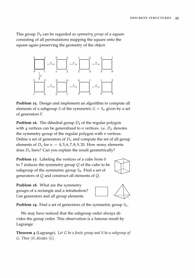
Example 18. We consider a particular subgroup D4 of the sym-metric group S4—called the dihedral group—which is generatedby two permutations π = (0, 1, 2, 3) and ρ = (0, 1)(2, 3):
D4 = 〈π, ρ〉.Iterated multiplication of π and ρ yields the following eightpermutations in D4:
ι = id4 ρ = (0, 1)(2, 3)
π = (0, 1, 2, 3) πρ = (0, 2)
π2 = (0, 2)(1, 3) π2ρ = (0, 3)(1, 2)
π3 = (0, 3, 2, 1) π3ρ = (1, 3)
discrete structures 49
This group D4 can be regarded as symmetry group of a squareconsisting of all permutations mapping the square onto thesquare again preserving the geometry of the object:
3 2
10
3
21
0
π
32
1
0
π
3
2 10
π
ρ
32
1 0
3
2 1
0
π
32
1
0
π
3
210
π
Problem 15. Design and implement an algorithm to compute allelements of a subgroup S of the symmetric G = Sn given by a setof generators Γ.
Problem 16. The dihedral group D4 of the regular polygonwith 4 vertices can be generalized to n vertices. i.e. Dn denotesthe symmetry group of the regular polygon with n vertices.Define a set of generators of Dn and compute the set of all groupelements of Dn for n = 4, 5, 6, 7, 8, 9, 20. How many elementsdoes Dn have? Can you explain the result geometrically?
Problem 17. Labeling the vertices of a cube from 0to 7 induces the symmetry group Q of the cube to besubgroup of the symmetric group S8. Find a set ofgenerators of Q and construct all elements of Q.
Problem 18. What are the symmetrygroups of a rectangle and a tetrahedron?List generators and all group elements.
Problem 19. Find a set of generators of the symmetric group Sn.
We may have noticed that the subgroup order always di-vides the group order. This observation is a famous result byLagrange:
Theorem 4 (Lagrange). Let G be a finite group and S be a subgroup ofG. Then |S| divides |G|.
50 michael braun
In order to prove this result we define a partition of the groupG induced by the subgroup S. We need this partition not onlyfor the proof but also for construction purpose in the latterchapters. If π ∈ G is a group element we define the (left) cosetπS := πρ | ρ ∈ S and the set of cosets
G/S := πS | π ∈ G.
The number of cosets |G/S| is sometimes called the index of asubgroup S in G and denoted by [G : S] or |G : S|.
It is easy to show that πS = σS if and only if π−1σ ∈ S.This connection defines an equivalence relation on G, i.e. π
and σ are equivalent if and only if π−1σ ∈ S is satisfied. Thecorresponding equivalence class of π ∈ G is exactly given bythe coset πS. Hence the cosets partition the group G. In additionsince by construction the cosets have all the same cardinality|πS| = |S| for all π ∈ G the number of cosets can be determinedby the ratio |G/S| = |G|/|S|. This proves Lagrange’s theorem.
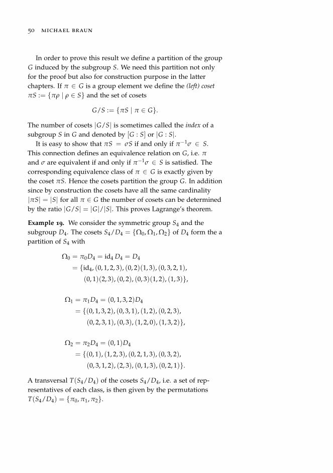
Example 19. We consider the symmetric group S4 and thesubgroup D4. The cosets S4/D4 = Ω0, Ω1, Ω2 of D4 form the apartition of S4 with
Ω0 = π0D4 = id4 D4 = D4
= id4, (0, 1, 2, 3), (0, 2)(1, 3), (0, 3, 2, 1),
(0, 1)(2, 3), (0, 2), (0, 3)(1, 2), (1, 3),
Ω1 = π1D4 = (0, 1, 3, 2)D4
= (0, 1, 3, 2), (0, 3, 1), (1, 2), (0, 2, 3),
(0, 2, 3, 1), (0, 3), (1, 2, 0), (1, 3, 2),
Ω2 = π2D4 = (0, 1)D4
= (0, 1), (1, 2, 3), (0, 2, 1, 3), (0, 3, 2),
(0, 3, 1, 2), (2, 3), (0, 1, 3), (0, 2, 1).
A transversal T(S4/D4) of the cosets S4/D4, i.e. a set of rep-resentatives of each class, is then given by the permutationsT(S4/D4) = π0, π1, π2.
discrete structures 51
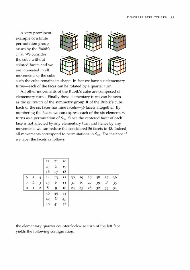
L U F
R D B
A very prominentexample of a finitepermutation grouparises by the Rubik’scube. We considerthe cube withoutcolored facets and weare interested in allmovements of the cubesuch the cube remains its shape. In fact we have six elementaryturns—each of the faces can be rotated by a quarter turn.
All other movements of the Rubik’s cube are composed ofelementary turns. Finally these elementary turns can be seenas the generators of the symmetry group R of the Rubik’s cube.Each of the six faces has nine facets—56 facets altogether. Bynumbering the facets we can express each of the six elementaryturns as a permutation of S56. Since the centered facet of eachface is not affected by any elementary turn and hence by anymovements we can reduce the considered 56 facets to 48. Indeed,all movements correspond to permutations in S48. For instance ifwe label the facets as follows
22 21 20
23 U 19
16 17 18
6 5 4 14 13 12 30 29 28 38 37 36
7 L 3 15 F 11 31 R 27 39 B 35
0 1 2 8 9 10 24 25 26 32 33 34
46 45 44
47 D 43
40 41 42
the elementary quarter counterclockwise turn of the left faceyields the following configuration:
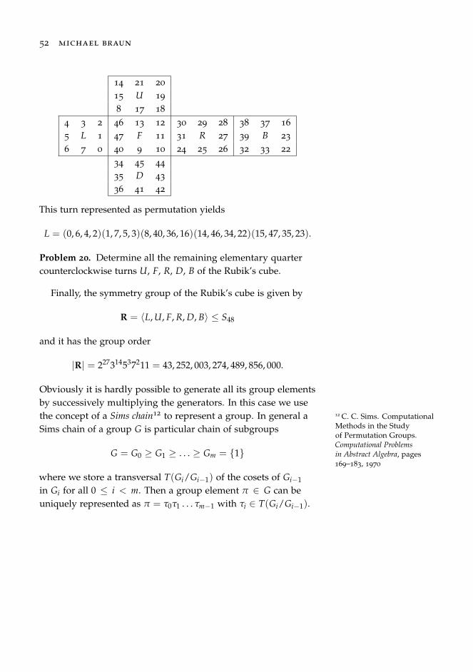
52 michael braun
14 21 20
15 U 19
8 17 18
4 3 2 46 13 12 30 29 28 38 37 16
5 L 1 47 F 11 31 R 27 39 B 23
6 7 0 40 9 10 24 25 26 32 33 22
34 45 44
35 D 43
36 41 42
This turn represented as permutation yields
L = (0, 6, 4, 2)(1, 7, 5, 3)(8, 40, 36, 16)(14, 46, 34, 22)(15, 47, 35, 23).
Problem 20. Determine all the remaining elementary quartercounterclockwise turns U, F, R, D, B of the Rubik’s cube.
Finally, the symmetry group of the Rubik’s cube is given by
R = 〈L, U, F, R, D, B〉 ≤ S48
and it has the group order
|R| = 227314537211 = 43, 252, 003, 274, 489, 856, 000.
Obviously it is hardly possible to generate all its group elementsby successively multiplying the generators. In this case we usethe concept of a Sims chain12 to represent a group. In general a 12 C. C. Sims. Computational
Methods in the Studyof Permutation Groups.Computational Problemsin Abstract Algebra, pages169–183, 1970
Sims chain of a group G is particular chain of subgroups
G = G0 ≥ G1 ≥ . . . ≥ Gm = 1
where we store a transversal T(Gi/Gi−1) of the cosets of Gi−1
in Gi for all 0 ≤ i < m. Then a group element π ∈ G can beuniquely represented as π = τ0τ1 . . . τm−1 with τi ∈ T(Gi/Gi−1).
discrete structures 53
Joseph-Louis de Lagrange (1736-1813) was afamous italian mathematician and astronomerwho made fundamental contributions to thearea of number theory, analysis, and mechan-ics laid the early foundations of group theory.
Alexandre Gustave Eiffel engraved thename of 21 french scientists in recognition of their significantcontributions on the Eiffel Tower—one name is Lagrange.
Later in 1830 the french mathematicianÉvariste Galois (1811-1832) who died youngat the age of twenty after a duel proposeda nonempty set G of permutations to be agroup if πρ ∈ G for all π, ρ ∈ G. He was thefirst mathematician to use the term group, heconstructed the finite field, and he introducedthe general linear group over a prime field—a
type of finite group we are going to use in a latter chapter.

Group actions
In the present chapter we consider group actions to partition a fi-nite set X of objects into equivalence classes. The correspondingequivalence classes arise by a given group G. In the followingwe assume G to be a multiplicatively written group with neutralelement 1G.
A mappingG× X → X, (π, x) 7→ πx
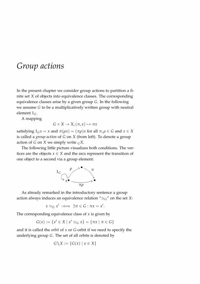
satisfying 1Gx = x and π(ρx) = (πρ)x for all π, ρ ∈ G and x ∈ Xis called a group action of G on X (from left). To denote a groupaction of G on X we simply write GX.
The following little picture visualizes both conditions. The ver-tices are the objects x ∈ X and the arcs represent the transition ofone object to a second via a group element:
•π
x•
ρ 55
πρ44
1G
++ •
As already remarked in the introductory sentence a groupaction always induces an equivalence relation “'G” on the set X:
x 'G x′ :⇐⇒ ∃π ∈ G : πx = x′.
The corresponding equivalence class of x is given by
G(x) := x′ ∈ X | x′ 'G x = πx | π ∈ Gand it is called the orbit of x or G-orbit if we need to specify theunderlying group G. The set of all orbits is denoted by
G\\X := G(x) | x ∈ X
56 michael braun
and yields a partition on X.The natural group action arises by a subgroup G the symmet-
ric group Sn on the set X = 0, . . . , n− 1 by
G× 0, . . . , n− 1 → 0, . . . , n− 1, (π, i) 7→ π(i).
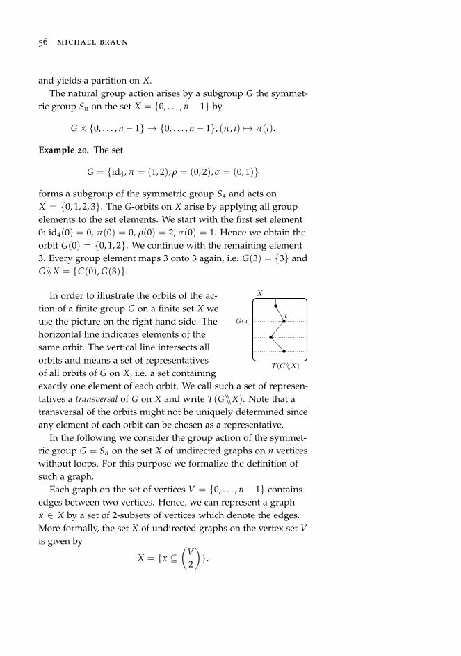
Example 20. The set
G = id4, π = (1, 2), ρ = (0, 2), σ = (0, 1)
forms a subgroup of the symmetric group S4 and acts onX = 0, 1, 2, 3. The G-orbits on X arise by applying all groupelements to the set elements. We start with the first set element0: id4(0) = 0, π(0) = 0, ρ(0) = 2, σ(0) = 1. Hence we obtain theorbit G(0) = 0, 1, 2. We continue with the remaining element3. Every group element maps 3 onto 3 again, i.e. G(3) = 3 andG\\X = G(0), G(3).
T (G\\X)
X
G(x)x
In order to illustrate the orbits of the ac-tion of a finite group G on a finite set X weuse the picture on the right hand side. Thehorizontal line indicates elements of thesame orbit. The vertical line intersects allorbits and means a set of representativesof all orbits of G on X, i.e. a set containingexactly one element of each orbit. We call such a set of represen-tatives a transversal of G on X and write T(G\\X). Note that atransversal of the orbits might not be uniquely determined sinceany element of each orbit can be chosen as a representative.
In the following we consider the group action of the symmet-ric group G = Sn on the set X of undirected graphs on n verticeswithout loops. For this purpose we formalize the definition ofsuch a graph.
Each graph on the set of vertices V = 0, . . . , n− 1 containsedges between two vertices. Hence, we can represent a graphx ∈ X by a set of 2-subsets of vertices which denote the edges.More formally, the set X of undirected graphs on the vertex set Vis given by
X = x ⊆(
V2
).
discrete structures 57
Another common characterization of the set of graphs on thevertex set V is given by
2(V2 ) :=
(V2
)→ 0, 1,
i.e. each possible 2-subset of V is identified with 1 or 0, meaning“edge” or “no edge”, respectively.
We remark that this definition immediately determines thenumber of graphs. We exactly have
2(n2) = 2
n(n−1)2
undirected graphs on n vertices without any loops.
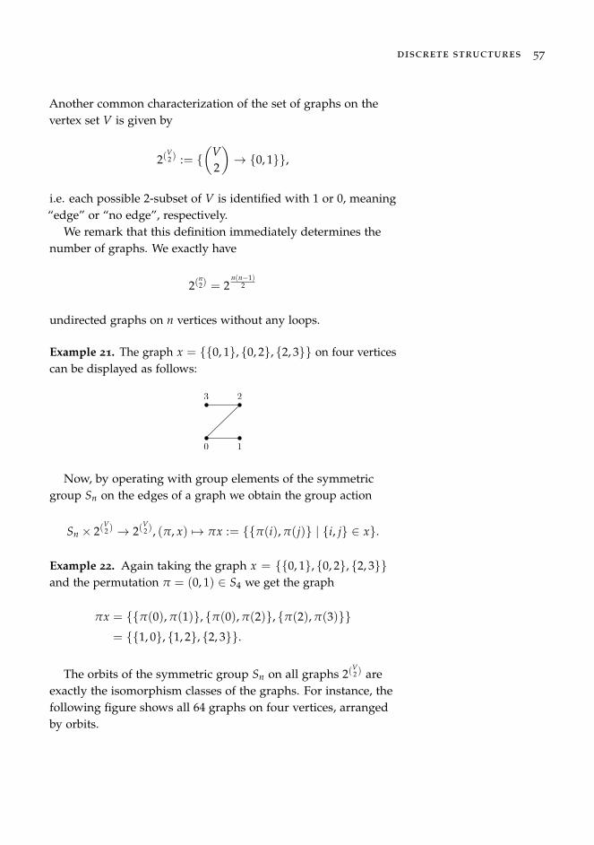
Example 21. The graph x = 0, 1, 0, 2, 2, 3 on four verticescan be displayed as follows:
3 2
10
Now, by operating with group elements of the symmetricgroup Sn on the edges of a graph we obtain the group action
Sn × 2(V2 ) → 2(
V2 ), (π, x) 7→ πx := π(i), π(j) | i, j ∈ x.
Example 22. Again taking the graph x = 0, 1, 0, 2, 2, 3and the permutation π = (0, 1) ∈ S4 we get the graph
πx = π(0), π(1), π(0), π(2), π(2), π(3)= 1, 0, 1, 2, 2, 3.
The orbits of the symmetric group Sn on all graphs 2(V2 ) are
exactly the isomorphism classes of the graphs. For instance, thefollowing figure shows all 64 graphs on four vertices, arrangedby orbits.
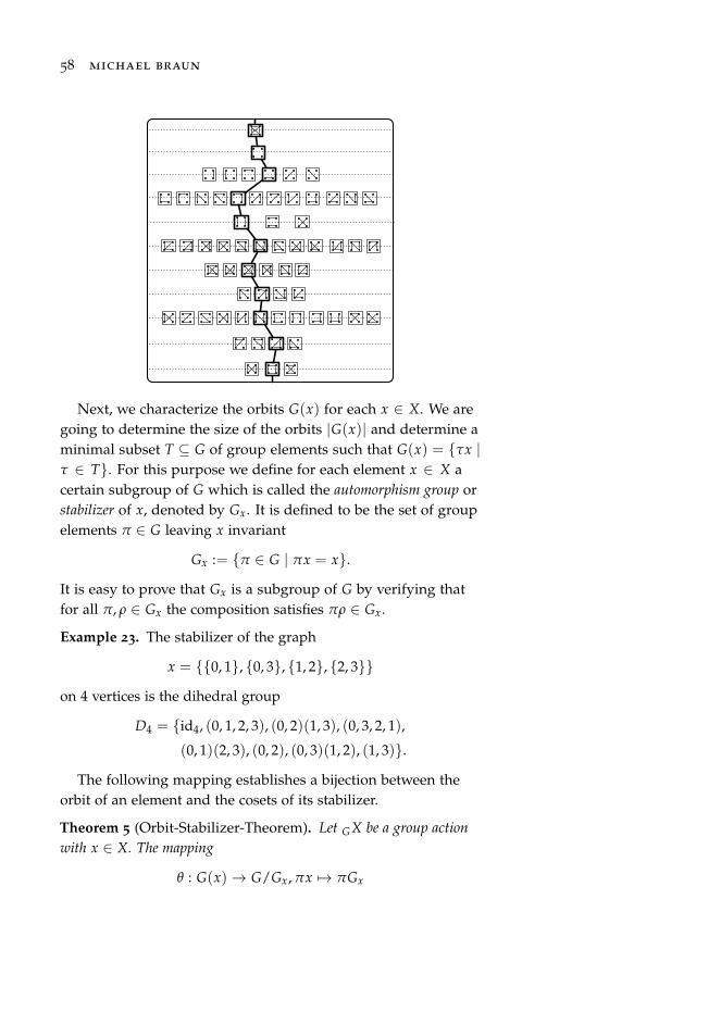
58 michael braun
Next, we characterize the orbits G(x) for each x ∈ X. We aregoing to determine the size of the orbits |G(x)| and determine aminimal subset T ⊆ G of group elements such that G(x) = τx |τ ∈ T. For this purpose we define for each element x ∈ X acertain subgroup of G which is called the automorphism group orstabilizer of x, denoted by Gx. It is defined to be the set of groupelements π ∈ G leaving x invariant
Gx := π ∈ G | πx = x.
It is easy to prove that Gx is a subgroup of G by verifying thatfor all π, ρ ∈ Gx the composition satisfies πρ ∈ Gx.
Example 23. The stabilizer of the graph
x = 0, 1, 0, 3, 1, 2, 2, 3
on 4 vertices is the dihedral group
D4 = id4, (0, 1, 2, 3), (0, 2)(1, 3), (0, 3, 2, 1),
(0, 1)(2, 3), (0, 2), (0, 3)(1, 2), (1, 3).
The following mapping establishes a bijection between theorbit of an element and the cosets of its stabilizer.
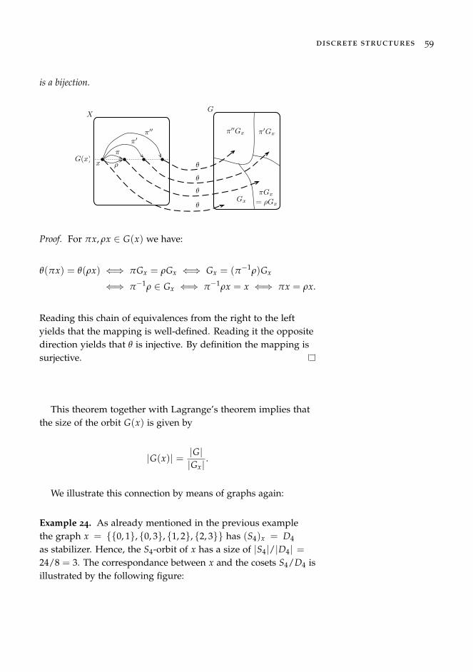
Theorem 5 (Orbit-Stabilizer-Theorem). Let GX be a group actionwith x ∈ X. The mapping
θ : G(x)→ G/Gx, πx 7→ πGx
discrete structures 59
is a bijection.
π
ρ
ππ
XG
πGxπGx
πGx
= ρGx
G(x)x θ
θ
θ
θGx
Proof. For πx, ρx ∈ G(x) we have:
θ(πx) = θ(ρx) ⇐⇒ πGx = ρGx ⇐⇒ Gx = (π−1ρ)Gx
⇐⇒ π−1ρ ∈ Gx ⇐⇒ π−1ρx = x ⇐⇒ πx = ρx.
Reading this chain of equivalences from the right to the leftyields that the mapping is well-defined. Reading it the oppositedirection yields that θ is injective. By definition the mapping issurjective.
This theorem together with Lagrange’s theorem implies thatthe size of the orbit G(x) is given by
|G(x)| = |G||Gx|
.
We illustrate this connection by means of graphs again:
Example 24. As already mentioned in the previous examplethe graph x = 0, 1, 0, 3, 1, 2, 2, 3 has (S4)x = D4
as stabilizer. Hence, the S4-orbit of x has a size of |S4|/|D4| =24/8 = 3. The correspondance between x and the cosets S4/D4 isillustrated by the following figure:
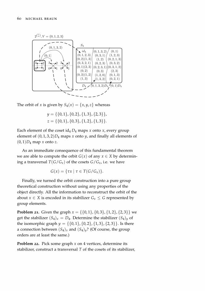
60 michael braun
id4
(0, 1, 2, 3)(0, 2)(1, 3)(0, 3, 2, 1)(0, 1)(2, 3)
(0, 2)(0, 3)(1, 2)
(1, 3)
(0, 1, 3, 2)(0, 3, 1)(1, 2)
(0, 2, 3)(0, 2, 3, 1)
(0, 3)(1, 2, 0)(1, 3, 2)
(0, 1)(1, 2, 3)
(0, 2, 1, 3)(0, 3, 2)
(0, 3, 1, 2)(2, 3)
(0, 1, 3)(0, 2, 1)
2(V2), V = 0, 1, 2, 3
S4
D4
(0, 1)
(0, 1, 3, 2)
(0, 1, 3, 2)D4 (0, 1)D4
3 2
10
3 2
10
3 2
10
The orbit of x is given by S4(x) = x, y, z whereas
y = 0, 1, 0, 2, 1, 3, 2, 3,z = 0, 1, 0, 3, 1, 2, 1, 3.
Each element of the coset id4 D4 maps x onto x, every groupelement of (0, 1, 3, 2)D4 maps x onto y, and finally all elements of(0, 1)D4 map x onto z.
As an immediate consequence of this fundamental theoremwe are able to compute the orbit G(x) of any x ∈ X by determin-ing a transversal T(G/Gx) of the cosets G/Gx, i.e. we have
G(x) = τx | τ ∈ T(G/Gx).
Finally, we turned the orbit construction into a pure grouptheoretical construction without using any properties of theobject directly. All the information to reconstruct the orbit of theabout x ∈ X is encoded in its stabilizer Gx ≤ G represented bygroup elements.
Problem 21. Given the graph x = 0, 1, 0, 3, 1, 2, 2, 3 weget the stabilizer (S4)x = D4. Determine the stabilizer (S4)y ofthe isomorphic graph y = 0, 1, 0, 2, 1, 3, 2, 3. Is therea connection between (S4)x and (S4)y? (Of course, the grouporders are at least the same.)
Problem 22. Pick some graph x on 4 vertices, determine itsstabilizer, construct a transversal T of the cosets of its stabilizer,
discrete structures 61
and determine the orbit of the chosen graph by means of thistransversal T. Verify your result by directly constructing the orbitof x.
A thorough introduction to the theory of finite group actionsoffers the book by Kerber13. 13 A. Kerber. Applied Finite
Group Actions. Springer-Verlag, 1999

Similar group actions
In the present chapter we consider the construction of orbitsof a particaluar type of group action by reducing the construc-tion problem in a pure group theoretical approach. We give anapplication in combinatorial chemistry.
We consider the same group G acting on two sets X and Zsuch that a bijection φ : X → Z exists commuting with the actionof H, i.e. it satisfies
φ(πx) = πφ(x)
for all x ∈ X and π ∈ G. In this case we call the both actions GXand GZ φ-similar and we write GX ≈φ GZ.
Lemma 6. Let GY and GZ be two φ-similar group actions. If T isa transversal of the orbits G\\Z then T′ = φ−1(z) | z ∈ T is atransversal of the orbits G\\X.
Proof. We show that φ maps the orbits of GX onto orbits of
GZ. For that reason transversals of G\\X will be mapped ontotransversals of G\\Z and vice versa. If x′ ∈ G(x) we get πx = x′
for some π ∈ G. Applying φ yields πφ(x) = φ(πx) = φ(x′)which means φ(x′) ∈ G(φ(x)).
An example of similar group actions arises by the Orbit-Stabilizer-Theorem saying that for any group action HY themapping
θ : H(y)→ H/Hy, πy 7→ πHy
is bijective for all all y ∈ Y. Now taking a subgroup G ≤ H andacting with its elements on the set X = H(y) ⊆ Y it splits intosmaller G-orbits. On the one hand we get the action
G× H(y)→ H(y), (ρ, πy) 7→ ρ(πy) = (ρπ)y
64 michael braun
and on the other hand
G× H/Hy → H/Hy, (ρ, πHy) 7→ ρ(πHy) = (ρπ)Hy.
which are similar G H(y) ≈θ G(H/Hy) via θ.
Corollary 3. Let HY be a group action, G ≤ H, and y ∈ H. Anytransversal T of the orbits G\\(H/Hy) yields a transversal of the orbitsG\\H(y) by T′ = θ−1(πHy) = πy | πHy ∈ T.
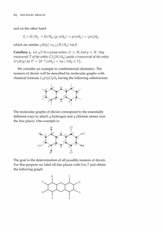
We consider an example in combinatorial chemistry: Theisomers of dioxin will be described by molecular graphs withchemical formula C12O2Cl4H4 having the following substructure:
O
O
C
C
C
C
C
C
CC
CC
C
C
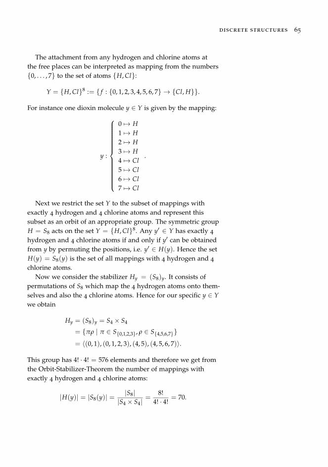
The molecular graphs of dioxin correspond to the essentiallydifferent ways to attach 4 hydrogen and 4 chlorine atoms overthe free places. One example is:
O
O
C
C
C
C
C
C
CC
CC
C
C
Cl
H
H
H
H
Cl
Cl
Cl
The goal is the determination of all possible isomers of dioxin.For this purpose we label all free places with 0 to 7 and obtainthe following graph:
0 1
2
3
45
6
7
discrete structures 65
The attachment from any hydrogen and chlorine atoms atthe free places can be interpreted as mapping from the numbers0, . . . , 7 to the set of atoms H, Cl:
Y = H, Cl8 := f : 0, 1, 2, 3, 4, 5, 6, 7 → Cl, H.
For instance one dioxin molecule y ∈ Y is given by the mapping:
y :
0 7→ H1 7→ H2 7→ H3 7→ H4 7→ Cl5 7→ Cl6 7→ Cl7 7→ Cl
.
Next we restrict the set Y to the subset of mappings withexactly 4 hydrogen and 4 chlorine atoms and represent thissubset as an orbit of an appropriate group. The symmetric groupH = S8 acts on the set Y = H, Cl8. Any y′ ∈ Y has exactly 4
hydrogen and 4 chlorine atoms if and only if y′ can be obtainedfrom y by permuting the positions, i.e. y′ ∈ H(y). Hence the setH(y) = S8(y) is the set of all mappings with 4 hydrogen and 4
chlorine atoms.Now we consider the stabilizer Hy = (S8)y. It consists of
permutations of S8 which map the 4 hydrogen atoms onto them-selves and also the 4 chlorine atoms. Hence for our specific y ∈ Ywe obtain
Hy = (S8)y = S4 × S4
= πρ | π ∈ S0,1,2,3, ρ ∈ S4,5,6,7= 〈(0, 1), (0, 1, 2, 3), (4, 5), (4, 5, 6, 7)〉.
This group has 4! · 4! = 576 elements and therefore we get fromthe Orbit-Stabilizer-Theorem the number of mappings withexactly 4 hydrogen and 4 chlorine atoms:
|H(y)| = |S8(y)| =|S8|
|S4 × S4|=
8!4! · 4!
= 70.
66 michael braun
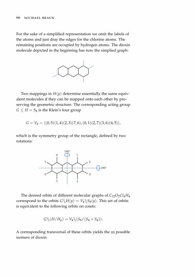
For the sake of a simplified representation we omit the labels ofthe atoms and just dray the edges for the chlorine atoms. Theremaining positions are occupied by hydrogen atoms. The dioxinmolecule depicted in the beginning has now the simplied graph:
Two mappings in H(y) determine essentially the same equiv-alent molecules if they can be mapped onto each other by pre-serving the geometric structure. The corresponding acting groupG ≤ H = S8 is the Klein’s four group
G = V4 = 〈(0, 5)(1, 4)(2, 3)(7, 6), (0, 1)(2, 7)(3, 6)(4, 5)〉,
which is the symmetry group of the rectangle, defined by tworotations:
0 1
2
3
45
6
7
180!
180!
The desired orbits of different molecular graphs of C12O2Cl4H4
correspond to the orbits G\\H(y) = V4\\S8(y). This set of orbitsis equivalent to the following orbits on cosets:
G\\(H/Hy) = V4\\(S8/(S4 × S4)).
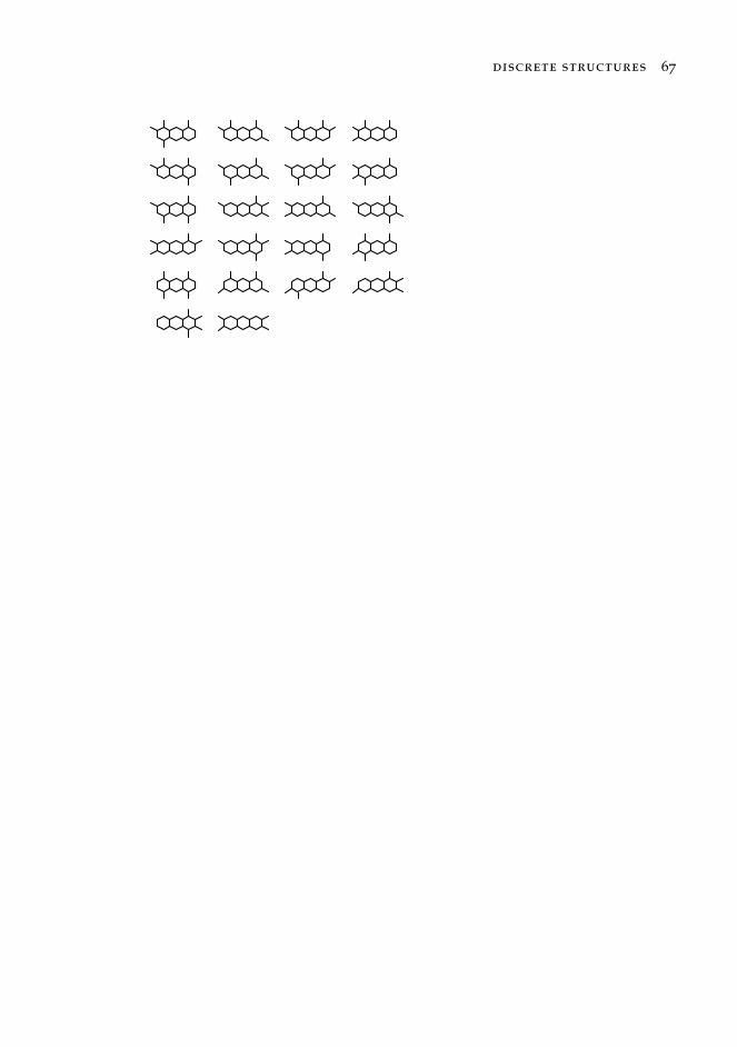
A corresponding transversal of these orbits yields the 22 possibleisomers of dioxin:
discrete structures 67

Orbit Evaluation
We consider the group action of a finite group G on a set X andwe want to evaluate the orbits of G on X. If G is a small groupthe orbit G(x) of x ∈ X can be constructed just by applyingall group elements π ∈ G to x. But quite often the group G isgiven by a set Γ ⊆ G of generators, i.e. G = 〈Γ〉. In this caseany group element π ∈ G can be expressed by a finite sequenceof generators π = γ0 . . . γ`−1, γi ∈ Γ for 0 ≤ i < `. Hence, itis sufficient to successively apply generators γ ∈ Γ to x and itsorbit elements reached from x by generators in order to constructthe whole orbit G(x). More formally, if we put
Ω0 := xΩ1 :=
⋃γ∈Γγx
Ωi := Ωi−1 ∪⋃
γ∈Γγx′ | x′ ∈ Ωi−1 \Ωi−2
, i ≥ 2
and construct the series of sets Ω0, Ω1, . . . until two subsequentsets are equal, Ωm = Ωm−1, we obtain G(x) = Ωm−1. Proceedingwith any x ∈ X\G(x) we can obtain further orbits until allelements of X are covered by orbits.
In the following we describe a concrete implementation ofthis way of evaluating the orbit G(x) utilizing a queue Q. Atthe beginning the queue Q holds the element x. In every stepwe remove the first element x′ of the queue Q and apply everygenerator γ ∈ Γ to x′. If by x′′ = γx′ we obtain a new notyet visited element of X we append x′′ to the queue Q. Thisprocedure will be repeated until the queue is empty and no new
70 michael braun
elements will added.Furthermore we store a group element as product of gener-
ators of Γ leading from x to any other element of its orbit. Dueto Orbit-Stabilizer-Theorem this set of group elements forms atransversal of the cosets G/Gx. To be more precise we also wantto determine a function α : G(x) → T(G/Gx) mapping anyorbit element x′′ ∈ G(x) onto the group element τ ∈ T(G/Gx)
such that x′′ = τx is satisfied. If x′′ = γx′ for any orbit ele-ment x′ ∈ G(x) and any generator γ ∈ Γ we obviously getx′′ = γx′ = γα(x′)x and hence we can define α(x′′) = γα(x′).
Finally we can formulate the following basic orbit algorithm.
Algorithmus 1. evaluation of orbit G(x)Input. Set Γ of generators of group G, x ∈ XOutput. G(x), α : G(x)→ T(G/Gx), τx 7→ τ
1 let Q be a queue holding x; Ω := x; α(x) := 1G
2 while Q 6= ∅ do3 let x′ be the first element of Q; remove x′ from Q4 for all γ ∈ Γ do5 x′′ := γx′
6 if x′′ 6∈ Ω do7 append x′′ to Q; Ω := Ω ∪ x′′; α(x′′) := γα(x′)8 return Ω, α
Problem 23. We consider the action of a permutation groupG ≤ Sn on the set X of k-subsets of 0, . . . , n − 1. ImplementAlgorithm 1 for this action. Think about an efficient implemen-tation: What is an appropriate data structure for Ω, Q and α?How can the test in line 6 be performed in O(1) operations? Is ithelpful to use rank and unrank functions for the k-subsets?
We illustrate the algorithm by giving a little example:
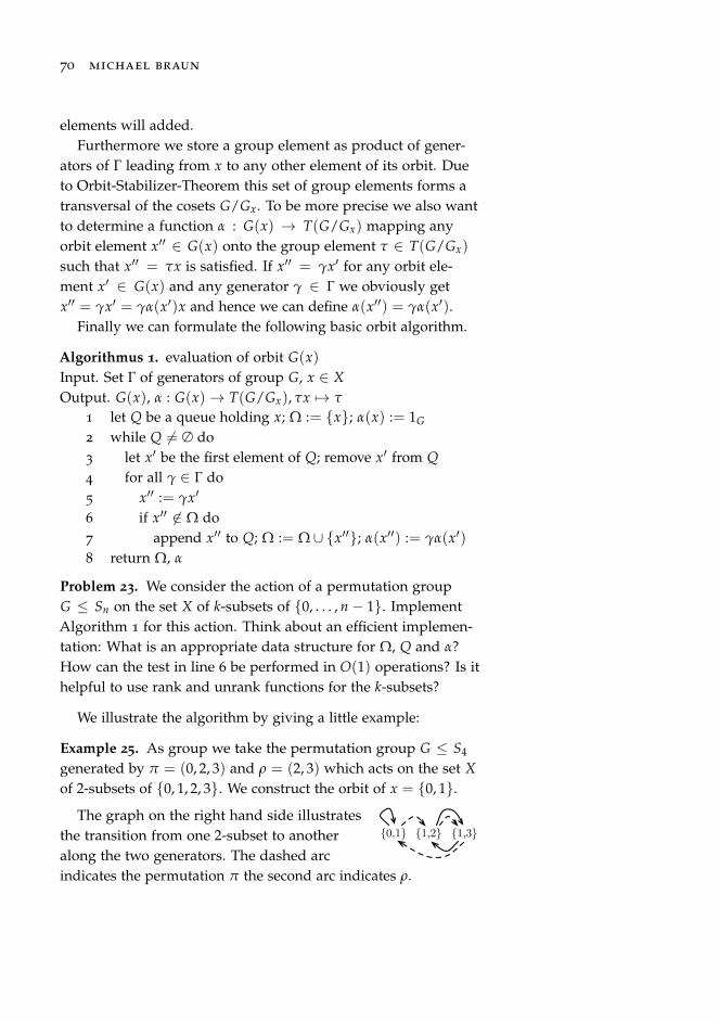
Example 25. As group we take the permutation group G ≤ S4
generated by π = (0, 2, 3) and ρ = (2, 3) which acts on the set Xof 2-subsets of 0, 1, 2, 3. We construct the orbit of x = 0, 1.
0,1 1,2 1,3The graph on the right hand side illustrates
the transition from one 2-subset to anotheralong the two generators. The dashed arcindicates the permutation π the second arc indicates ρ.
discrete structures 71
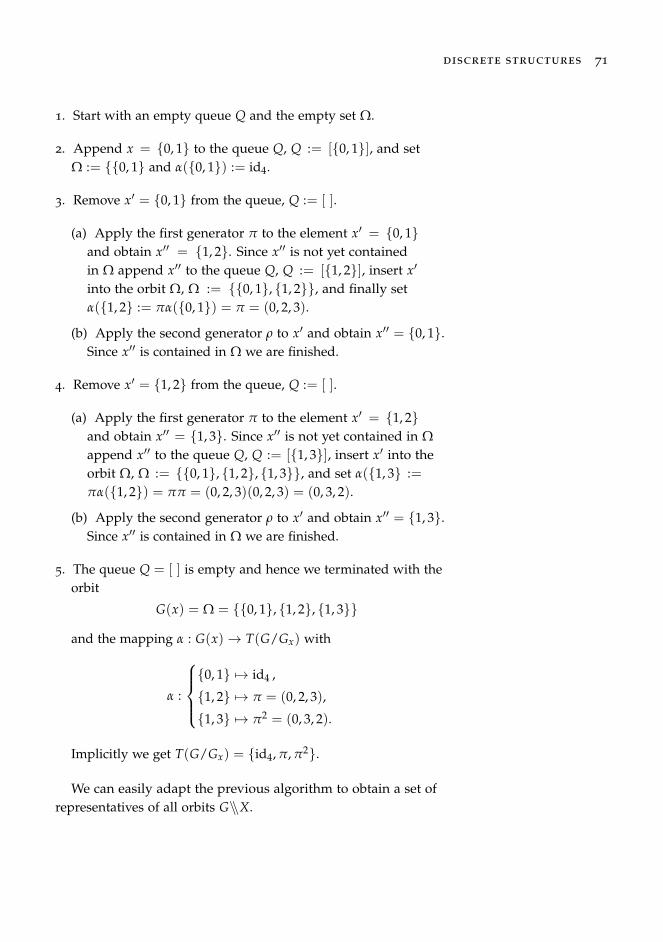
1. Start with an empty queue Q and the empty set Ω.
2. Append x = 0, 1 to the queue Q, Q := [0, 1], and setΩ := 0, 1 and α(0, 1) := id4.
3. Remove x′ = 0, 1 from the queue, Q := [ ].
(a) Apply the first generator π to the element x′ = 0, 1and obtain x′′ = 1, 2. Since x′′ is not yet containedin Ω append x′′ to the queue Q, Q := [1, 2], insert x′
into the orbit Ω, Ω := 0, 1, 1, 2, and finally setα(1, 2 := πα(0, 1) = π = (0, 2, 3).
(b) Apply the second generator ρ to x′ and obtain x′′ = 0, 1.Since x′′ is contained in Ω we are finished.
4. Remove x′ = 1, 2 from the queue, Q := [ ].
(a) Apply the first generator π to the element x′ = 1, 2and obtain x′′ = 1, 3. Since x′′ is not yet contained in Ωappend x′′ to the queue Q, Q := [1, 3], insert x′ into theorbit Ω, Ω := 0, 1, 1, 2, 1, 3, and set α(1, 3 :=πα(1, 2) = ππ = (0, 2, 3)(0, 2, 3) = (0, 3, 2).
(b) Apply the second generator ρ to x′ and obtain x′′ = 1, 3.Since x′′ is contained in Ω we are finished.
5. The queue Q = [ ] is empty and hence we terminated with theorbit
G(x) = Ω = 0, 1, 1, 2, 1, 3
and the mapping α : G(x)→ T(G/Gx) with
α :
0, 1 7→ id4 ,
1, 2 7→ π = (0, 2, 3),
1, 3 7→ π2 = (0, 3, 2).
Implicitly we get T(G/Gx) = id4, π, π2.
We can easily adapt the previous algorithm to obtain a set ofrepresentatives of all orbits G\\X.
72 michael braun
Algorithmus 2. transversal of orbits T(G\\X)
Input. Set Γ of generators of group G, XOutput. T(G\\X)
1 ∆ := X; T := ∅2 while ∆ 6= ∅ do3 let x be an element of ∆; ∆ := ∆ \ x4 let Q be a queue holding x; T := T ∪ x5 while Q 6= ∅ do6 let x′ be the first element of Q; remove x′ from Q7 for all γ ∈ Γ do8 x′′ := γx′
9 if x′′ ∈ ∆ do10 append x′′ to Q; ∆ := ∆ \ x′′11 return T
Problem 24. We again consider the action of a permutation groupG ≤ Sn on the set X of k-subsets of 0, . . . , n − 1. ImplementAlgorithm 2 for this action. What data structure is reasonable for∆?
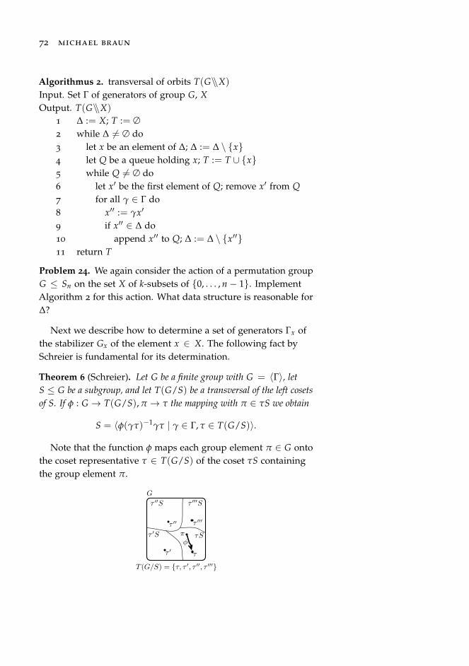
Next we describe how to determine a set of generators Γx ofthe stabilizer Gx of the element x ∈ X. The following fact bySchreier is fundamental for its determination.
Theorem 6 (Schreier). Let G be a finite group with G = 〈Γ〉, letS ≤ G be a subgroup, and let T(G/S) be a transversal of the left cosetsof S. If φ : G → T(G/S), π → τ the mapping with π ∈ τS we obtain
S = 〈φ(γτ)−1γτ | γ ∈ Γ, τ ∈ T(G/S)〉.
Note that the function φ maps each group element π ∈ G ontothe coset representative τ ∈ T(G/S) of the coset τS containingthe group element π.
G
τSτ S
τ S τ S
π
T (G/S) = τ, τ , τ , τ
φ
ττ
τ τ
discrete structures 73
We now apply this theorem to the situation that the subgroupS of G is the stabilizer of x, i.e. S = Gx. So far we computed theorbit G(x) and the mapping α : G(x) → T(G/Gx), τx 7→ τ butwe need the mentioned mapping φ : G → T(G/Gx) to obtain aset of generators
Γx = φ(γτ)−1γτ | γ ∈ Γ, τ ∈ T(G/Gx)
of the stabilizer Gx = 〈Γx〉. From the Orbit-Stabilizer-Theoremwe get for π ∈ G and τ ∈ T(G/Gx) the equivalence
π ∈ τGx ⇐⇒ πx = τx ⇐⇒ α(πx) = τ.
This defines the required mapping
φ : G → T(G/Gx) : π 7→ α(πx)
and we get a set Γx of generators of Gx by
Γx = α(γτx)−1γτ | γ ∈ Γ, τ ∈ T(G/Gx).
Problem 25. We refer to Problem 23. Extend this implementationsuch that a set of generators for the stabilizer of any k-subset of0, . . . , n− 1 can be computed.
A classical book on algorithms for permutation groups andgroup actions is by Butler14. The book by Seress15 also offers an 14 G. Butler. Fundamental
Algorithms for PermutationGroups. Springer BerlinHeidelberg, 1991
15 Á. Seress. PermutationGroup Algorithms. CambridgeUniversity Press, 2003
extensive treatment of algorithms.A proof of Schreier’s theorem can be found in16.
16 A. Betten, M. Braun,H. Fripertinger, A. Kerber,A. Kohnert, and A. Wasser-mann. Error CorrectingLinear Codes. Classificationby Isometry and Applications,volume 18 of Algorithms andComputation in Mathematics(ACM). Springer-Verlag,Berlin Heidelberg NewYork, 2006; and A. Kerber.Applied Finite Group Actions.Springer-Verlag, 1999

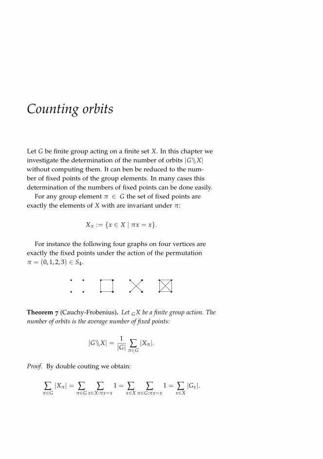
Counting orbits
Let G be finite group acting on a finite set X. In this chapter weinvestigate the determination of the number of orbits |G\\X|without computing them. It can ben be reduced to the num-ber of fixed points of the group elements. In many cases thisdetermination of the numbers of fixed points can be done easily.
For any group element π ∈ G the set of fixed points areexactly the elements of X with are invariant under π:
Xπ := x ∈ X | πx = x.
For instance the following four graphs on four vertices areexactly the fixed points under the action of the permutationπ = (0, 1, 2, 3) ∈ S4.
Theorem 7 (Cauchy-Frobenius). Let GX be a finite group action. Thenumber of orbits is the average number of fixed points:
|G\\X| = 1|G| ∑
π∈G|Xπ |.
Proof. By double couting we obtain:
∑π∈G|Xπ | = ∑
π∈G∑
x∈X:πx=x1 = ∑
x∈X∑
π∈G:πx=x1 = ∑
x∈X|Gx|.
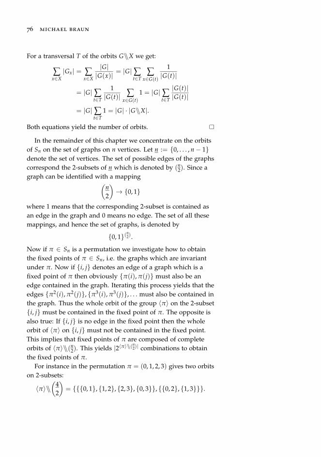
76 michael braun
For a transversal T of the orbits G\\X we get:
∑x∈X|Gx| = ∑
x∈X
|G||G(x)| = |G|∑t∈T
∑x∈G(t)
1|G(t)|
= |G|∑t∈T
1|G(t)| ∑
x∈G(t)1 = |G|∑
t∈T
|G(t)||G(t)|
= |G|∑t∈T
1 = |G| · |G\\X|.
Both equations yield the number of orbits.
In the remainder of this chapter we concentrate on the orbitsof Sn on the set of graphs on n vertices. Let n := 0, . . . , n− 1denote the set of vertices. The set of possible edges of the graphscorrespond the 2-subsets of n which is denoted by (n
2). Since agraph can be identified with a mapping(
n2
)→ 0, 1
where 1 means that the corresponding 2-subset is contained asan edge in the graph and 0 means no edge. The set of all thesemappings, and hence the set of graphs, is denoted by
0, 1(n2).
Now if π ∈ Sn is a permutation we investigate how to obtainthe fixed points of π ∈ Sn, i.e. the graphs which are invariantunder π. Now if i, j denotes an edge of a graph which is afixed point of π then obviously π(i), π(j) must also be anedge contained in the graph. Iterating this process yields that theedges π2(i), π2(j), π3(i), π3(j), . . . must also be contained inthe graph. Thus the whole orbit of the group 〈π〉 on the 2-subseti, j must be contained in the fixed point of π. The opposite isalso true: If i, j is no edge in the fixed point then the wholeorbit of 〈π〉 on i, j must not be contained in the fixed point.This implies that fixed points of π are composed of completeorbits of 〈π〉\\(n
2). This yields |2〈π〉\\(n2)| combinations to obtain
the fixed points of π.For instance in the permutation π = (0, 1, 2, 3) gives two orbits
on 2-subsets:
〈π〉\\(
42
)= 0, 1, 1, 2, 2, 3, 0, 3, 0, 2, 1, 3.
discrete structures 77
Combining thes two orbits defines the four graphs
∅,
0, 1, 1, 2, 2, 3, 0, 3,0, 2, 1, 3,0, 1, 1, 2, 2, 3, 0, 3, 0, 2, 1, 3.
Corollary 4. The number of isomorphism classes of graphs on nvertices is given by
|Sn\\0, 1(n2)| = 1
n! ∑π∈Sn
2|〈π〉\\(n2)|.
Obviously two permutations π, ρ ∈ Sn with the same cycletype t produce the same number of orbits on 2-subsets andhence the same number of fixed points. Instead of calculating thenumber of fixed points for each permutation in Sn it is sufficientto determine this number of permutations of different cyclecycles. With the results of Chapter 5 we obtain (the notationt a n means a cycle type of the number n):
Corollary 5. The number of isomorphism classes of graphs on nvertices is given by
|Sn\\0, 1(n2)| = ∑
t an
2|〈πt〉\\(n2)|
∏ni=1 iti ti!
where πt ∈ Sn is a permutation of the cycle type t.
For example we compute the number of isomorphism classesof undirected graphs on four vertices. First we determine the dif-ferent cycle types t of the number n = 4, calculate ∏n
i=1 iti ti!, givepermutations πt with the corresponding cycle type t , compute|〈πt〉\\(n
2)|, and finally evaluate the number of orbits:
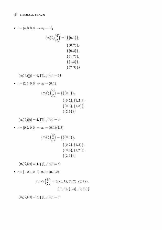
78 michael braun
• t = [4, 0, 0, 0] ⇒ πt = id4
〈πt〉\\(
42
)= 0, 1,
0, 2,0, 3,1, 2,1, 3,2, 3
|〈πt〉\\(42)| = 6, ∏n
i=1 iti ti! = 24
• t = [2, 1, 0, 0] ⇒ πt = (0, 1)
〈πt〉\\(
42
)= 0, 1,
0, 2, 1, 2,0, 3, 1, 3,2, 3
|〈πt〉\\(42)| = 4, ∏n
i=1 iti ti! = 4
• t = [0, 2, 0, 0] ⇒ πt = (0, 1)(2, 3)
〈πt〉\\(
42
)= 0, 1,
0, 2, 1, 3,0, 3, 1, 2,2, 3
|〈πt〉\\(42)| = 4, ∏n
i=1 iti ti! = 8
• t = [1, 0, 1, 0] ⇒ πt = (0, 1, 2)
〈πt〉\\(
42
)= 0, 1, 1, 2, 0, 2,
0, 3, 1, 3, 2, 3
|〈πt〉\\(42)| = 2, ∏n
i=1 iti ti! = 3
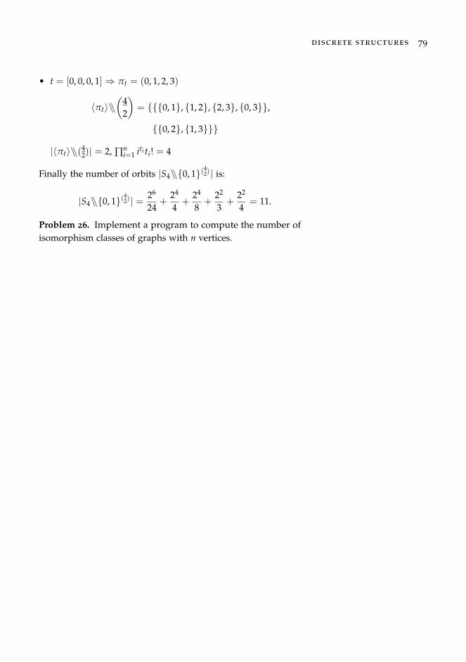
discrete structures 79
• t = [0, 0, 0, 1] ⇒ πt = (0, 1, 2, 3)
〈πt〉\\(
42
)= 0, 1, 1, 2, 2, 3, 0, 3,
0, 2, 1, 3
|〈πt〉\\(42)| = 2, ∏n
i=1 iti ti! = 4
Finally the number of orbits |S4\\0, 1(42)| is:
|S4\\0, 1(42)| = 26
24+
24
4+
24
8+
22
3+
22
4= 11.
Problem 26. Implement a program to compute the number ofisomorphism classes of graphs with n vertices.

Bibliography
[1] A. Betten, M. Braun, H. Fripertinger, A. Kerber, A. Kohnert,and A. Wassermann. Error Correcting Linear Codes. Classifica-tion by Isometry and Applications, volume 18 of Algorithms andComputation in Mathematics (ACM). Springer-Verlag, BerlinHeidelberg New York, 2006.
[2] G. Butler. Fundamental Algorithms for Permutation Groups.Springer Berlin Heidelberg, 1991.
[3] F. Gray. Pulse Code Communication. U.S. Patent 2,632,058,March 1953 (filed Nov. 1947).
[4] S. M. Johnson. Generation of Permutations by AdjacentTranspositions. Mathematics of Computations, 17:382–285, 1963.
[5] A. Kerber. Applied Finite Group Actions. Springer-Verlag, 1999.
[6] D. E. Knuth. The Art of Computer Programming, Volume 4,Fascicle 2: Generating All Tuples and Permutations. Addison-Wesley, 2005.
[7] D. E. Knuth. The Art of Computer Programming, Volume 4,Fascicle 3: Generating All Combinations and Partitions. Addison-Wesley, 2005.
[8] D. L. Kreher and D. R. Stinson. Combinatorial Algorithms—Generation, Enumeration, and Search. CRC Press, 1999.
[9] A. Nijenhuis and H. S. Wilf. Combinatorial Algorithms.Academic Press, Inc., London, 1978.
[10] Á. Seress. Permutation Group Algorithms. CambridgeUniversity Press, 2003.
82 michael braun
[11] C. C. Sims. Computational Methods in the Study of Permu-tation Groups. Computational Problems in Abstract Algebra,pages 169–183, 1970.
[12] G. Stibitz. Binary Counter. U.S. Patent 2,307,868, 1943.
[13] H. F. Trotter. PERM (Algorithm 115). Communications of theACM, 5:434–435, 1962.
Index
q-binomial coefficient, 27
action, 10
group, 8
automorphism group, 9
binary reflected Gray code,16
Binomial coefficient, 19
cardinality, 12
Cauchy-Frobenius formula,9
chainSims, 52
characteristic vector, 11
coefficientq-binomial, 27
Gaussian, 27
complement, 12
cycle denotation, 39
cycle type, 40
deletion, 12
denotationcycle, 39
list, 33
distance, 15
Hamming, 16
enumerative generation, 11,14
equivalent, 10
Gaussian coefficient, 27
generationenumerative, 11, 14
graph isomorphism, 7
Grassmannian, 27
Gray codebinary reflected, 16
group, 10
action, 10
automorphism, 9
multiplicative, 47
symmetric, 47
group action, 8, 10
Hamming distance, 16
insertion, 12
integer partition, 42
intersection, 12
isomorphic, 10
isomorphism, 10
graph, 7
84 michael braun
lexicographic ordering, 13
list denotation, 33
membership test, 12
minimal change ordering, 15
multiplicative group, 47
orderinglexicographic, 13
minimal change, 15
partition, 9, 42
Pascal’s identity, 19
Pascal’s triangle, 19
permutation, 9, 33
predecessor, 15
rank, 13, 14
set, 9
Sims chain, 52
subset, 9
subspace, 9
successor, 13, 14
symmetric group, 47
symmetry, 9
testmembership, 12
transposition, 39
union, 12
unrank, 14
vectorcharacteristic, 11