Discussion Papers in Economics

No. 2000/62

Dynamics of Output Growth, Consumption and Physical Capital in Two-Sector Models of Endogenous Growth

by

Farhad Nili

Department of Economics and Related Studies University of York

Heslington York, YO10 5DD

No. 2000/61

Short Term and Long Term Effects of Price Cap Regulation

by

Gianni De Fraja and Alberto Iozzi

Short Term and Long Term E¤ects

of Price Cap Regulation

Gianni De Fraja¤

University of York

and C.E.P.R.

Alberto Iozziy

Università di Roma

Tor Vergata

December 5, 2000

Abstract

This paper uses a very simple example (two goods, linear symmet-

ric demand and cost) to study the e¤ects of the price cap regulatory

mechanism. We show that if a given price vector is preferred (using

current welfare as the criterion) to another, then it is not necessarily

the case that it is also preferred in the long run (using the presented

discounted value of welfare as the criterion). The relationship between

current welfare and pro…t and therefore the …rm’s incentive to bargain

for a given price vector depend on the speci…c details of the mechanism

considered.

JEL Numbers: I28, D63

Keywords: Ramsey prices, Price cap regulation.¤University of York, Department of Economics and Related Studies, Heslington,

York Y010 5DD and C.E.P.R., 90-98 Goswell Street, London EC1V 7DB; email:

gd4@york.ac.uk.yUniversità di Roma Tor Vergata, Dip. SEFEMEQ, Via di Tor Vergata, I-00151, Rome,

Italy; email: Alberto.Iozzi@UniRoma2.It.

1 Introduction

Price cap regulation rates as one of the success stories of applied economic

theory. The reason is probably the fact that it strikes a very good com-

promise between the theoretically rigorous foundation of the theory of op-

timal regulation for multiproduct …rms (detailed in Jean-Jacques La¤ont

and Jean Tirole [12], ch.3) and the practitioner’s requirement of the simple,

easy-to-understand, easy-to-apply rule. Price cap regulation works in the-

ory, because the model upon which it is based captures in an ad hoc, but

nonetheless sound, fashion the asymmetry of information which is after all

the very reason why regulation is needed. Price cap regulation also works in

practice, because, in view of its simplicity, is applicable to situations where

the regulated …rm has hundreds of di¤erent prices, as can well be the case

for telecommunication companies, but retains desirable properties with re-

gard to both productive e¢ciency (as it does not distort a …rm’s incentives

for cost reduction because the …rm is the residual claimant of any e¢ciency

gain), and allocative e¢ciency (as it reduces relative price distortions and

the monopoly dead-weight loss). The success of price cap regulation is re-

‡ected in the large number of countries across the world that have adopted

this principle for the regulation of multiproduct …rms (OECD [13]).

A price cap mechanism has two basic, conceptually distinct, constituent

elements:

² an initial price vector, and

² an adjustment mechanism.

The general principle is that, in any given period, the regulated …rm can

only choose prices which belong to a set of permitted prices (Michael Beesley

and Steve Littlechild [5], Mark Armstrong, Simon Cowan and John Vickers

[1] and Vickers [15]). In some cases, this set is independent of the …rm’s

1

behaviour in the previous periods and is simply decided by the regulator at

the beginning of the regulatory period. In general, it has been shown that

this type of price cap has undesirable properties with respect to allocative

e¢ciency (Ian Bradley and Catherine Price [8], Armstrong and Vickers [3]

and Cowan [10] and [11]). If instead the set of permitted prices in any period

is calculated using an adjustment mechanism based on the prices charged by

the …rm in the previous period, the mechanism is called dynamic price cap.

We concentrated on this case in this paper.

The adjustment mechanism for dynamic price cap regulation has received

a good deal of theoretical attention. An earlier analysis was carried out by

Ingo Vogelsang and Jorg Finsinger [17], who proposed the following mecha-

nism. In any period, the regulated …rm is required to set prices such that,

if these prices were applied to the quantities sold in the previous period, the

…rm would incur a loss. Vogelsang and Finsinger assume that the …rm is

myopic, namely that, in every period, it chooses the vector of prices that

maximise its current pro…t under the constraint. Their main …nding is that

the sequence of prices chosen by the …rm converges to the allocatively e¢-

cient (second best) Ramsey prices with zero pro…ts (that is the prices where,

for each good, the price mark-up above marginal cost is proportional to the

reciprocal of the demand elasticity for that good and where total revenues

equal total cost) (Frank Ramsey [14], Marcel Boiteaux [7] and William Bau-

mol and David Bradford [4]).

A di¤erent mechanism is proposed by Timothy Brennan [9]. It requires

the …rm to set in every period of time prices such that a Laspeyres price

index (which uses appropriate weights) is less than 1. This is the mechanism

adopted in the typical RPI-X mechanism, adopted for the regulation of most

utilities in, among others, the UK.1 In this case also, the sequence of prices

1The mechanism requires the price of a given basket of goods sold by the regulated …rm

not to increase in a given year by more that (RPI-X), where RPI is the retail price index

2

charged by a myopic regulated …rm converges to second-best prices that

obey the Ramsey rule. The two mechanisms display very similar properties.

There is, however, one fundamental di¤erence between them. The Brennan

mechanisms is such that the …rm’s pro…ts increase over time, while in the

Vogelsang and Finsinger mechanism pro…t tends to zero. This di¤erence is

re‡ected in the level of the prices charged by the …rm in the long run, in

both cases they obey the Ramsey rule, but are lower in the Vogelsang and

Finsinger mechanism.

While the long-term properties are clearly important, regulators (and

their principals, the politicians) are also likely to be concerned with the short

term properties of the regulatory mechanism. Thus, for example, in the prac-

tical debate, much attention has been devoted to the speci…c reduction in

the Laspeyres price index that regulated …rms should be required: the X in

the RPI-X formula (Je¤rey Bernstein and David Sappington [6]). Also im-

portant, in practice, is the period for which this number is …xed (Armstrong,

Ray Rees and Vickers [2]).

The …rst element of the price cap mechanism, the initial price vector, has

received much less attention. This is perhaps not surprising; from a theoret-

ical point of view the dynamic properties of the adjustment mechanism are

clearly more interesting than the “given” initial condition of the dynamical

system. In practice, initial prices have typically been those prevailing at the

beginning of the regulatory process, often following the privatisation of the

state monopoly, when the presence of something …xed and given was proba-

bly welcome by all involved, given the host of other variables that had to be

bargained over and agreed upon.

However, in industries where technological change is rapid, and where,

increase for that year and X is a number agreed at the review of the regulatory agreement.

If (RPI-X) is negative, that is, for X high relative to in‡ation, this price of the basket of

goods is, of course, required to decrease by at least (RPI-X).

3

for example, new products are introduced regularly, it may be necessary

occasionally to “restart” as it were, the regulatory mechanism, by choosing

a new, di¤erent, initial price vector. The existing theoretical literature gives

little or no guidance on the consequences of choosing a new initial price

vector. In this paper, we address a very simple, but important, question

in this respect. Speci…cally, we investigate whether, given two initial price

vectors, it is the case that the initial price vector which is preferable in the

current period (in the sense that it gives a higher score under the chosen

welfare criterion) is also preferable along the path of convergence to the

Ramsey prices (in the sense that it has a higher discounted present value of

the score under the same welfare criterion). We show, by means of a simple,

but nonetheless robust, example, that the answer to this question is negative,

both for the Vogelsang and Finsinger and the Brennan mechanisms. This

may have important implications if and when initial prices are renegotiated

or otherwise reset. For example, suppose that the regulated …rm asks the

regulators to be allowed to charge prices which (i) violate the constraints

imposed by the mechanism, but (ii) are preferred (in current term) by the

regulator, to the existing prices. Our simple example suggests that, contrary

to what one might expect, the regulator should not, in general, allow such

prices, before a more thorough analysis of their consequences is carried out.

Even in the extremely simple examples we consider (two identical goods,

linear independent demands, linear cost), it is possible that the regulated

…rm may propose a price vector that makes the regulator better o¤ in the

short term but worse o¤ in the medium and long-term. Succinctly, prices

leading to higher welfare in the short run may turn out to lead to lower

welfare in the long run. More importantly, the nature of the regulatory

mechanism is important in providing the …rm with the incentive to propose

the new initial prices: in our simple example, under the Brennan mechanism,

there exist price vectors such that the …rm is better o¤ in proposing a change

4

which makes the regulator better o¤ in the short term but worse o¤ in the

long term. This, in our example, does not happen with the Vogelsang and

Finsinger mechanism.

The plan of this note is the following: in Section 2 we describe schemati-

cally the model of dynamic price cap regulation, and in Section 3 we propose

a simple example which illustrates the short and long run e¤ects of the initial

prices.

2 The General Model of Price Cap Regula-

tion

The broad outline of the general framework for the analysis of price cap

regulation is given by the following set of assumptions:

² There exist M markets which are open over an in…nite number of time

periods, t = 1; :::;1. In each period of time t, the M -dimensional

vector of continuous and downward sloping market demand functions

is q = q(pt), where p = (p1; :::; pM) is the price vector, with pi the price

of good i, and q = (q1; :::; qM), with qi the quantity of good i. Demand

functions are invariant over time, and satisfy standard assumptions.

² A multiproduct monopolistic …rm produces the M goods in each pe-

riod. Production costs are denoted by c(q), which it is assumed to be

continuously di¤erentiable and constant over time.

² The …rm is myopic: in each period t = 1; :::;1 it maximises its current

pro…ts.

² Preferences of society are represented by the welfare function W (p),

which is assumed to be continuously di¤erentiable and quasi-convex.

5

² The regulator agency does not have the power directly to set the prices

of the goods produced by the …rm, but can o¤er the …rm a regulatory

contract.

² The contract o¤ered to the …rm entails that the …rm is free to choose

the prices it may prefer, provided that in any period of time t = 1; :::;1they satisfy a constraint whose general form is given by:

I = I(pt;pt¡1) � 1: (1)

² We denote by pI = pI(p) any price vector which constitutes the limit

of the sequence of prices which, in each period, maximises the current

pro…t, subject to constraint (1), given that the initial price vector is p.

Note that this vector need not be unique, and therefore, in general, pI

need not be a function.

In Vogelsang and Finsinger [17], the index I takes the following form:

I = V (pt;pt¡1) =

PMi=1 qi(p

t¡1)ptic(q(pt¡1))

: (2)

That is, if the quantity of each good sold in the previous period had

been sold at today price then the …rm would not have covered its total

cost. Vogelsang and Finsinger show that from any initial price vector p,

the sequence of prices charged by the …rm converges to the price vector

which maximises the consumers’ surplus under the constraint of non-negative

pro…ts for the …rm. That is, pV (p) = p0R, where p0R are the zero-pro…t

Ramsey prices. Under reasonable conditions, this vector is unique, implying

that from any initial conditions, the mechanism is such that, in the long

run equilibrium the …rm earns zero pro…ts, and consumers enjoy the highest

possible welfare compatible with the …rm breaking-even.

Brennan [9] relaxes some of the restrictive assumptions on the …rm’s tech-

nology used by Vogelsang and Finsinger and imposes a less stringent price

6

cap constraint. In his paper, the …rm faces a price cap constraint given by a

standard Laspeyres price index:

I = B(pt;pt¡1) =

PMi=1 qi(p

t¡1)ptiPMi=1 qi(p

t¡1)pt¡1i

: (3)

From an informational point of view, (3), unlike (2), does not require

knowledge of the actual cost incurred, which could be an advantage when

the …rm also operates in markets outside the regulator’s remit, and it is not

possible to check the internal cost allocation between divisions of the …rm.

Brennan shows that the consumers surplus is weakly increasing over time

and that the sequence of prices converges to a Ramsey price vector in the

long run equilibrium. However, the pro…ts enjoyed by the …rms are also

increasing over time and at the beginning of the regulatory process it is not

possible to predict or control the level of pro…ts the …rm will obtain in the

long run equilibrium, unless, of course, the cost function is also known to the

regulator. Moreover, clearly, the pro…t earned by the …rm in the limit under

the Brennan mechanism is strictly positive.

3 Long-run and short-run properties

The contribution of this note is to show that a new price vector that, in

the current period improves welfare may lower it in the long term. In other

words, that the relationship between short term and long term welfare is

not monotonic. For the sake of de…niteness, we take welfare to be given by

consumers’ surplus, so that

W (p) =

Z¢ ¢ ¢

Zq1(x):::qM(x)dx1:::dxM :

Long term welfare WL(p), naturally, is given by the discounted sum of

all future welfare levels. If fpt(p0)g1t=1 is the sequence of prices charged by

7

the …rm, when the initial price is p0, then:

WL(p0) = lims!1

Xs

t=0±tW (pt(p0)):

Formally we establish the following results.

Proposition 1 (Vogelsang and Finsinger mechanism). Let the …rm be

subject to price cap regulation, under the constraint (2). W (p0) < W (pV )

does not imply WL(p0) < WL(pV )

Proposition 2 (Brennan mechanism). Let the …rm be subject to price

cap regulation, under the constraint (3). W (p0) < W (pB) does not imply

WL(p0) < WL(pB), nor does it imply W (p(p0)) < W (p(pB)).

In words, it is not necessarily the case that the price vector which guar-

antees higher welfare in the short run has also the same property in the long

run equilibrium.

Note the di¤erence between the two mechanisms: with both mechanisms

the present discounted value of the welfare can be lower, but, with the Bren-

nan mechanism, it may also happen that of the limit value of the welfare is

also lower. This, clearly, cannot happen with the Vogelsang and Finsinger

mechanism, given that, irrespective of the initial prices, convergence is to the

price vector which has the Ramsey property and zero pro…t. As we will see,

this a¤ects the …rms incentives to propose new prices.

To establish the results, it is su¢cient to exhibit numerical examples; we

take a simple example. Given our aim, the simpler the example the better:

more complex situation have simpler situations as special cases, and therefore

a simple example implies a more general result. Our example is also robust:

there are two goods, M = 2, and in both markets demand is linear. The cost

function is also linear and symmetric: c(q1; q2) = c (q1 + q2) + F . There is

no further loss in generality in normalising demand so that q1 = 1¡ p1 and

q2 = 1¡ p2.

8

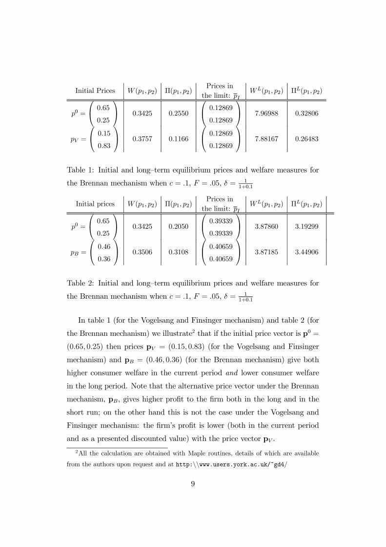
Initial Prices W (p1; p2) ¦(p1; p2)Prices in

the limit: pIWL(p1; p2) ¦L(p1; p2)

p0 =

0@ 0:65

0:25

1A 0.3425 0.2550

0@ 0:12869

0:12869

1A 7.96988 0.32806

pV =

0@ 0:15

0:83

1A 0.3757 0.1166

0@ 0:12869

0:12869

1A 7.88167 0.26483

Table 1: Initial and long–term equilibrium prices and welfare measures for

the Brennan mechanism when c = :1, F = :05, ± = 11+0:1

Initial prices W (p1; p2) ¦(p1; p2)Prices in

the limit: pIWL(p1; p2) ¦L(p1; p2)

p0 =

0@ 0:65

0:25

1A 0.3425 0.2050

0@ 0:39339

0:39339

1A 3.87860 3.19299

pB =

0@ 0:46

0:36

1A 0.3506 0.3108

0@ 0:40659

0:40659

1A 3.87185 3.44906

Table 2: Initial and long–term equilibrium prices and welfare measures for

the Brennan mechanism when c = :1, F = :05, ± = 11+0:1

In table 1 (for the Vogelsang and Finsinger mechanism) and table 2 (for

the Brennan mechanism) we illustrate2 that if the initial price vector is p0 =

(0:65; 0:25) then prices pV = (0:15; 0:83) (for the Vogelsang and Finsinger

mechanism) and pB = (0:46; 0:36) (for the Brennan mechanism) give both

higher consumer welfare in the current period and lower consumer welfare

in the long period. Note that the alternative price vector under the Brennan

mechanism, pB, gives higher pro…t to the …rm both in the long and in the

short run; on the other hand this is not the case under the Vogelsang and

Finsinger mechanism: the …rm’s pro…t is lower (both in the current period

and as a presented discounted value) with the price vector pV .

2All the calculation are obtained with Maple routines, details of which are available

from the authors upon request and at http:nnwww.users.york.ac.uk/~gd4/

9

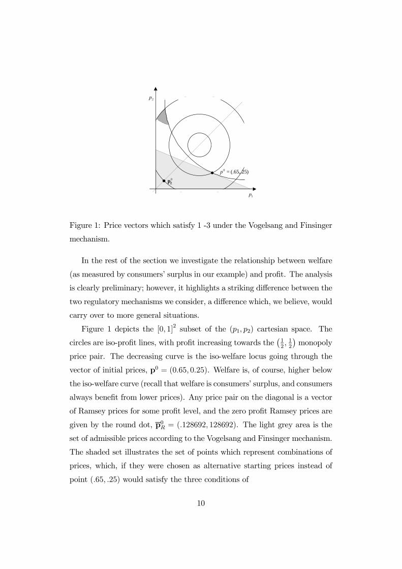
)25,.65(.0 =p

1p

2p

0Rp

Figure 1: Price vectors which satisfy 1 -3 under the Vogelsang and Finsinger

mechanism.

In the rest of the section we investigate the relationship between welfare

(as measured by consumers’ surplus in our example) and pro…t. The analysis

is clearly preliminary; however, it highlights a striking di¤erence between the

two regulatory mechanisms we consider, a di¤erence which, we believe, would

carry over to more general situations.

Figure 1 depicts the [0; 1]2 subset of the (p1; p2) cartesian space. The

circles are iso-pro…t lines, with pro…t increasing towards the¡12; 12

¢monopoly

price pair. The decreasing curve is the iso-welfare locus going through the

vector of initial prices, p0 = (0:65; 0:25). Welfare is, of course, higher below

the iso-welfare curve (recall that welfare is consumers’ surplus, and consumers

always bene…t from lower prices). Any price pair on the diagonal is a vector

of Ramsey prices for some pro…t level, and the zero pro…t Ramsey prices are

given by the round dot, p0R = (:128692; 128692). The light grey area is the

set of admissible prices according to the Vogelsang and Finsinger mechanism.

The shaded set illustrates the set of points which represent combinations of

prices, which, if they were chosen as alternative starting prices instead of

point (:65; :25) would satisfy the three conditions of

10

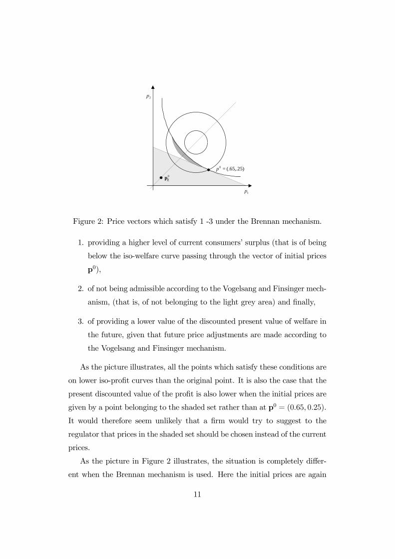
1p

2p

0Rp

)25,.65(.0 =p

Figure 2: Price vectors which satisfy 1 -3 under the Brennan mechanism.

1. providing a higher level of current consumers’ surplus (that is of being

below the iso-welfare curve passing through the vector of initial prices

p0),

2. of not being admissible according to the Vogelsang and Finsinger mech-

anism, (that is, of not belonging to the light grey area) and …nally,

3. of providing a lower value of the discounted present value of welfare in

the future, given that future price adjustments are made according to

the Vogelsang and Finsinger mechanism.

As the picture illustrates, all the points which satisfy these conditions are

on lower iso-pro…t curves than the original point. It is also the case that the

present discounted value of the pro…t is also lower when the initial prices are

given by a point belonging to the shaded set rather than at p0 = (0:65; 0:25).

It would therefore seem unlikely that a …rm would try to suggest to the

regulator that prices in the shaded set should be chosen instead of the current

prices.

As the picture in Figure 2 illustrates, the situation is completely di¤er-

ent when the Brennan mechanism is used. Here the initial prices are again

11

p0 = (0:65; 0:25). Again the shaded set represent combinations of points

which are not admissible according to the Brennan mechanism, which give

a higher value of current welfare, and a lower present discounted value of

future welfare. Note, however, that the …rm is better o¤ when the prices are

given by points in the shaded set, which are inside the circle representing the

iso-pro…t locus to which p0 belongs. The present discounted value of pro…t

is also higher along the path which is followed by the prices which would be

chosen by the …rm starting from a point inside the shaded set and following

the Brennan mechanism.

These two diagrams, therefore, would suggest radical di¤erence di¤erences

in the behaviour of the two pricing mechanisms in the simple set up of our

example; these di¤erences are not due to any special feature of our example,

and should carry through to more general examples.

Speci…cally, the Vogelsang and Finsinger mechanism, is such that in order

for a pair of price pV to give both higher current welfare and lower present

discounted value of welfare than the existing prices p0, they must be, in a

loose sense, more distorded from Ramsey prices than the exisiting prices:

since welfare at the end of the convergence process is the same with both

price pairs, and since prices pV have higher welfare at the beginning of the

convergence process than prices p0, then welfare must be lower for some

intermediate period of time, when the convergence process start from pV . For

this to happen, the convergence process must be less speedy, which occurs,

as it were, when there is more distance to travel to reach the Ramsey prices

obtained at the end of the convergence process.

The opposite occurs when the adjustment mechanism is given by the

Brennan mechanism. Here prices which give a higher consumers’ surplus

than prices p0 are prices closer to the Ramsey prices for some pro…t level

(namely along the diagonal, where p1 = p2). A price pair pB in the shaded

set is closer to the prices which will be eventually chosen period after period

12

by a …rm regulated according to the Brennan mechanism. This is because

the prices eventually chosen depend themselves on the initial prices, unlike

the prices to which the Vogelsang and Finsinger mechanism converges. By

choosing prices closer to Ramsey prices the …rm is able to speed up the

convergence process, and therefore make it converge to higher prices, which

therefore give higher pro…ts.

4 Conclusion

We present here an exceedingly simple example, which, despite its simplicity

has an important lesson for regulators. The details of the regulatory mech-

anism matter considerably for the achievement of the regulator’s objective.

Should a …rm propose to restart the price cap regualtory mechanism with

a di¤erent a new price it is possible that prices which are preferable from

the regualtor’s viewpoint when compared to the existing prices will make the

regulator worse o¤ in the long period.

In our elementary example, the …rms’ incentives to suggest such prices

are stronger when the price cap formula is based on a Laspeyres price index,

(based on Brennan’s [9] original suggestion).

13

References

[1] Armstrong, M., Cowan, S. and Vickers, J. (1994). Regulatory Reform.

Cambridge (MA): MIT Press.

[2] Armstrong, M., Rees, R. and Vickers, J. (1994). Optimal regulatory lag

under price cap regulation. Revista Española de Economia, 0, Special

Issue 1995, 93-116.

[3] Armstrong, M. and Vickers, J. (1991). Welfare e¤ects of price discrimina-

tion by a regulated monopolist. Rand Journal of Economics, 22, 571-80.

[4] Baumol, W. J. and Bradford, D. F. (1970). Optimal departures from

marginal cost pricing. American Economic Review, 60, 265-83.

[5] Beesley, M. E. and Littlechild, S. C. (1989). The regulation of privatised

monopolies in the UK. Rand Journal of Economics, 20, 454-72.

[6] Bernstein, J.I. and Sappington D.E.M. (1999). Setting the X factor in

price-cap regulation plans. Journal of Regulatory Economics, (1) 5-25.

[7] Boiteux, M. (1956). Sur la gestion des monopoles publics astreints à

l’équilibre budgétarie. Econometrica, 22, 22-40. English version: (1971).

On the management of Public Monopolies subject to budgetary con-

straints. Journal of Economic Theory, 3, 219-240.

[8] Bradley, I. and Price, C. (1988). The economic regulation of private in-

dustries by price constraints. Journal of Industrial Economics, XXXVII,

99-106.

[9] Brennan, T. J. (1989). Regulating by capping prices. Journal of Regu-

latory Economics, 1, 133-47.

[10] Cowan, S. (1997). Price-cap regulation and ine¢ciency in relative pric-

ing. Journal of Regulatory Economics, 12, 53-70.

14

[11] Cowan, S. (1997). Tighter average revenue regulation can be worse than

no regulation. Journal of Industrial Economics, XLV, 75-88.

[12] La¤ont, J.-J. and Tirole, J. (1993). A Theory of Incentives in Procure-

ment and Regulation. Cambridge (MA): MIT Press.

[13] OECD (2000). Economic Outlook no. 67. Paris: OECD.

[14] Ramsey, F. P. (1927). A contribution to the theory of taxation. Economic

Journal, 37, 47-61.

[15] Vickers, J. (1997). Regulation, competition, and the structure of prices.

Oxford Review of Economic Policy, 13 (1), 15-26.

[16] Vogelsang, I. (1989). Price cap regulations of telecommunications ser-

vices: A Long-Run Approach. in Crew, M. A. (ed.). Deregulation and

Diversi…cation of Utilities. Boston: Kluwer Academic Publishers.

[17] Vogelsang, I. and Finsinger, J. (1979). A regulatory adjustment process

for optimal pricing by multiproduct monopoly …rms. Bell Journal of

Economics, 10, 157-71.

15