Disjoint Paths in Densely Embedded Graphs

Jon Kleinberg∗ Eva Tardos†

October, 1995

Abstract

We consider the following maximum disjoint paths problem (mdpp). We are givena large network, and pairs of nodes that wish to communicate over paths through thenetwork — the goal is to simultaneously connect as many of these pairs as possiblein such a way that no two communication paths share an edge in the network. Thisclassical problem has been brought into focus recently in papers discussing applicationsto routing in high-speed networks, where the current lack of understanding of the mdpp

is an obstacle to the design of practical heuristics.We consider the class of densely embedded, nearly-Eulerian graphs, which includes

the two-dimensional mesh and many other planar and locally planar interconnectionnetworks. We obtain a constant-factor approximation algorithm for the maximum dis-joint paths problem for this class of graphs; this improves on an O(log n)-approximationfor the special case of the two-dimensional mesh due to Aumann–Rabani and the au-thors. For networks that are not explicitly required to be “high-capacity,” this is thefirst constant-factor approximation for the mdpp in any class of graphs other thantrees.

We also consider the mdpp in the on-line setting, relevant to applications in whichconnection requests arrive over time and must be processed immediately. Here weobtain an asymptotically optimal O(log n)-competitive on-line algorithm for the sameclass of graphs; this improves on an O(log n log log n)-competitive algorithm for thespecial case of the mesh due to Awerbuch, Gawlick, Leighton, and Rabani.

1 Introduction

We consider the following maximum disjoint paths problem (mdpp). We are given a largenetwork, and pairs of nodes that wish to communicate over paths through the network —the goal is to simultaneously connect as many of these pairs as possible in such a way that

∗E-mail: kleinber@theory.lcs.mit.edu. Laboratory for Computer Science, MIT, Cambridge MA 02139USA. Supported by an ONR Graduate Fellowship.

†E-mail: eva@cs.cornell.edu. School of ORIE, Cornell University, Ithaca NY 14853. Supported in partby a Packard Fellowship and an NSF PYI award.

1

no two communication paths share an edge in the network. This problem is well-known tobe computationally difficult. Deciding whether all pairs can be so connected is one of Karp’soriginal NP-complete problems [12]; it remains NP-complete even when the underlying graphis the two-dimensional mesh [15].

Our interest in this problem comes from two main sources. First, establishing disjointpaths is fundamental to routing in high-speed networks (see for example the applicationsmentioned in [6, 8, 21], as well as applications to optical routing in [1, 3, 24]). Although thetypes of routing problems that arise in such settings tend to have additional side constraints(e.g. connections have limited duration and can bring varying amounts of “profit”), theformulation described in the first paragraph contains the essence of virtually all such real-life routing problems in which each connection consumes a large fraction of the bandwidthon a link. As such, the current lack of understanding of the disjoint paths problem is amajor obstacle to the design of practical heuristics. Indeed, [6] notes that in practice, thegreedy algorithm tends to be used for routing, despite its bad performance on a numberof very common interconnection patterns. Moreover, robust ways are known for convertingalgorithms for the mdpp into algorithms that can handle connections of limited duration orvariable value [5]; thus, the difficulties contained in these more elaborate routing problemsseem to stem mainly from the intractability of the mdpp.

This problem is also of basic interest in algorithmic graph theory. A lot of work hasbeen done on identifying special cases of the disjoint paths problem that can be solved inpolynomial time, or for which simple min-max conditions can be stated; see the survey byFrank [10]. Much less work has been done, however, on approximation algorithms for themdpp; we are interested in extending the classes of graphs for which good approximationscan be obtained.

1.1 Our Results

To be precise, let G = (V,E) be a graph on n vertices and T = (s1, t1), . . . , (sk, tk) acollection of terminal pairs — pairs of vertices of G. We say that T is realizable in G ifthere exist mutually edge-disjoint si-ti paths, for i = 1, . . . , k. The problem is then to find arealizable subset of T of maximum cardinality.

Our first main result is a constant-factor approximation for the maximum disjoint pathsproblem in the class of densely embedded, nearly-Eulerian graphs (defined below), whichincludes many common planar and locally planar interconnection networks. This improveson an O(logn)-approximation for the case of the two-dimensional mesh due to Aumann andRabani [3] and an O(logn)-approximation for a class of planar graphs including the meshdue to the authors [14]. Our present algorithm makes use of variants of a number of thetechniques developed in our earlier paper [14].

The assumption that we know all the terminal pairs in advance is not reasonable insituations in which connection requests between pairs of nodes arrive over time and mustbe processed immediately. In such a setting, it makes sense to consider on-line routingalgorithms. Such an algorithm is given the graph G, terminal pairs arrive in an arbitraryorder, and for each such pair it must irrevocably reject it, or assign it a path in G. As

2

is standard, we refer to the approximation ratio achieved by an on-line algorithm as itscompetitive ratio; such an algorithm is said to be c-competitive if its competitive ratio is atmost c.

Our second main result, then, is an O(logn)-competitive randomized on-line algorithm forthe mdpp in densely embedded, nearly-Eulerian graphs. This improves on anO(logn log log n)-competitive algorithm for the special case of the two-dimensional mesh due to Awerbuch,Gawlick, Leighton, and Rabani [6]; moreover, [6] proves that no randomized on-line algo-rithm for the two-dimensional mesh can be better than Ω(log n)-competitive, implying thatour algorithm is asymptotically optimal.

We feel that an important feature of our algorithms, in addition to the improved bounds,is that they are not specific to the mesh; the advantage of developing algorithms that workon the somewhat larger class of “densely embedded graphs” is that are not sensitive to smallvariations in the structure of the underlying graph. This could be of value in the context ofnetwork routing, where the underlying network may have a “mesh-like” topology, but lackthe completely regular structure of the mesh. In contrast, previous algorithms such as [6, 3]could not be applied to any network other than the mesh itself, since they required its fixedrow/column structure.

The size of the constants in our algorithms as presented here, while not astronomical,pushes them outside the range of immediate practical utility. However, the previous bestbounds — both off-line and on-line — for the two-dimensional mesh [3, 6, 14] involve similarlylarge constants inside the O(·) notation. Moreover, despite the large constants, some of theideas used by the algorithms here may be of use in suggesting practical heuristics.

The rest of the paper is organized as follows. First, we present some preliminary algo-rithmic tools that we need in Section 2. Our routing algorithms are simpler to explain inthe special case of the mesh, and we consequently present this case first. This will be donein Section 3. In Section 4, we then introduce the class of densely embedded graphs, andwe present the algorithms for this class in Section 5. Finally, we show how to extend ouralgorithms to a slightly more general class of graphs in Section 6.

1.2 Previous Work

Much of the previous work on this problem has dealt with the case in which each pathconsumes only a small fraction of the available bandwidth on an edge; this can be modeledby requiring Ω(log n) parallel copies of each edge. In this case, the randomized roundingtechnique of Raghavan and Thompson [23, 22] can be used to obtain an off-line constant-factor approximation. Awerbuch, Azar, and Plotkin give an on-line O(logn)-competitivealgorithm for this case [4], which they show is asymptotically tight for deterministic on-linealgorithms.

As noted in [6] however, there are many applications in which each communication pathconsumes a large fraction of the available bandwidth on a link; thus it makes sense to con-sider approximation algorithms for graphs without a large number of parallel edges. Theresults here are much more restricted. For trees with parallel edges, Garg, Vazirani, and Yan-nakakis [11] obtain an off-line 2-approximation (the maximization problem is NP-complete,

3

though deciding realizability is easy); Awerbuch et. al. [6] give an O(log d)-competitive ran-domized on-line algorithm for trees of diameter d, extending an earlier result of Awerbuchet. al. [5]. Essentially the only approximation results known for graphs other than trees arethose mentioned earlier for the mesh and related planar graphs [3, 6, 14]. Thus our resulthere is the first constant-factor approximation for any class of graphs other than trees, whenone does not require Ω(log n) parallel copies of each edge.

A different approach is taken in papers of Peleg and Upfal [21] and Broder, Frieze, andUpfal [8] (see also Broder et. al. [7]). Here the underlying graph G is assumed to havestrong expansion properties; in this case one can prove that any set of terminal pairs of atmost a given size must be realizable in G, and that corresponding paths can be found in(randomized) polynomial time. The results in [8] are strong enough that they implicitlyprovide a polylogarithmic approximation for the mdpp in sufficiently strong expanders ofbounded degree.

In this context, it is worth mentioning the following closely related routing problem:one must route all terminal pairs so as to minimize the maximum congestion on any edge;that is, the maximum number of paths that contain an edge. Deciding whether T can berouted with congestion equal to 1 is the same as deciding whether T is realizable; but as anoptimization problem, minimizing congestion is much better understood. Aspnes et al. [2]give an on-line O(logn)-competitive algorithm for the problem; and a randomized roundingalgorithm of Raghavan and Thompson [23] gives a routing off-line with congestion at mostOPT + o(OPT ) +O(logn), where OPT denotes the optimum congestion. This leaves openthe question of whether a constant-factor approximation is achievable also for small values ofOPT . In a companion paper with Satish Rao [13], we give a constant-factor approximationfor densely embedded graphs; it was here that the idea of using a “simulated network” (seeSection 3) was initially developed.

Cases in which the mdpp can be solved in polynomial time are surveyed in [10]; herewe only discuss two specific results that we will use in handling densely embedded graphs.First, suppose G is planar, the terminals T lie on a single face of G, and the pair (G, T )satisfies the following parity condition: the augmented graph formed by adding to G the edgescorresponding to T must be Eulerian. In this case, a theorem of Okamura and Seymour [20]says that the realizability of T in G can be decided in polynomial time; and in fact thefollowing cut condition is sufficient for realizability: one cannot remove j edges from G andseparate more than j terminal pairs. A linear-time algorithm for this problem has recentlybeen obtained by Wagner and Weihe [30]. We will use an extension of the Okamura–Seymour,due to Frank [9], which concerns the case in which the parity condition does need not tohold on the face containing the terminals.

We also use a theorem of Schrijver [28] that provides an algorithm for finding vertex-disjoint paths in a graph embedded on a compact surface Σ, such that the paths satisfy givenhomotopy constraints.

4

2 Preliminary Tools

2.1 The AAP Algorithm

We make use of a variant of an on-line mdpp algorithm of Awerbuch, Azar, and Plotkin [4]. IfH is a graph with n nodes in which each edge has capacity at least log 2n, the algorithm of [4]achieves a competitive ratio of 2 log 4n. For our purposes, we need to develop a strengtheningof this “AAP algorithm”: we want to be competitive against the fractional optimum; andwhen we deal with the more general case of densely embedded graphs, we want only torequire capacities to be ε logn, for an arbitrary ε > 0. Here, we show how to obtain such analgorithm.

Proposition 2.1 If all edge capacities are at least (ε logn+ 1 + ε), there is a deterministicon-line mdpp algorithm that is O(21/ε log n)-competitive against the fractional optimum.

Proof. We follow the AAP algorithm and its analysis very closely. We vary a little fromtheir notation, since we only deal here with routing a maximal number of requests, each ofinfinite duration. Thus, the ith request is specified by a pair (si, ti) of terminals. We definethe “profit” of the connection to be n; thus the total profit obtained by the on-line algorithmis simply n times the number of terminal pairs routed.

Define µ = 21+1/εn, so we have

ε logµ = ε logn+ 1 + ε.

Let ue denote the capacity of edge e; thus we can assume that for all e,

ue ≥ ε logµ.

With this value of µ, we now run the AAP algorithm — for the sake of completeness, westate this algorithm here.

For j = 1, 2, . . . , k:Define λje to be the fraction of ue consumed by paths already routed.

Define cje = ue(µλj

e − 1).For a request (si, ti), route it on any path P satisfying

∑

e∈P1uecje ≤ n.

If no such path is available, then reject the request.

First we argue why the relative load on an edge will never exceed 1. At the momentbefore this happened, on edge e say, we had

λje > 1 − 1

ue≥ 1 − 1

ε logµ.

5

Thus

cjeue

= µλje − 1

> µ1− 1ε log µ − 1

=µ

21/ε− 1 = 2n− 1

≥ n.

So we havecjeue

> n

and thus the connection could not have used this edge.Suppose there are a total of k requests. Let A denote the set of requests routed by the

AAP algorithm. Then we show

21+1/ε log µ∑

j∈A

n ≥∑

e

ck+1e . (1)

As in the proof in [4] we show this by induction on the number of admitted requests, viaproving that if the algorithm admits the jth request, we have

∑

e

cj+1e − cje ≤ 21+1/εn logµ.

So consider edge e on the jth path used by the AAP algorithm. We have

cj+1e − cje = ue

(

µλje(2(log µ)/ue − 1)

)

.

Now the exponent on the 2 is at most 1/ε, and for x ∈ [0, 1/ε] we clearly have 2x−1 ≤ 21/ε ·x.Thus

cj+1e − cje ≤ ue · µλ

je · 21/ε · (log µ)/ue

= µλje · 21/ε · logµ

= 21/ε · log µ ·[

cjeue

+ 1

]

.

Summing over all edges gives the desired bound.Finally, we show that the expression

∑

e

ck+1e (2)

is an upper bound on the profit of the fractional optimum minus the profit of the on-linealgorithm. ([4] shows this for the integer optimum, but the proof is essentially the same.)

6

Let Q denote the set of indices which were rejected by the on-line algorithm but forwhich a positive fraction of the demand was routed by the optimum. For j ∈ Q, supposethat the fractional optimum uses paths P 1

j , . . . , Pzj , with weights γ1

j , . . . , γzj . Then since j

was rejected by the on-line algorithm, and the costs are monotonic in the indices, we musthave

n ≤∑

e∈P ij

ck+1e

ue

for any i, j. Then for any edge e we have

∑

i,j:e∈P ij

γijue

≤ 1,

and hence we have

∑

j

∑

i

γijn ≤∑

j

∑

i

∑

e∈P ij

γijck+1e

ue

≤∑

e

ck+1e ·

∑

i,j:e∈P ij

γijue

≤∑

e

ck+1e .

Combining the bounds in Equations (1) and (2), we obtain the claimed competitive ratio.

A lower bound of [4] implies that the factor of 21/ε is unavoidable for deterministic on-linealgorithms.

2.2 Combining On-Line Algorithms

In routing connections on-line, we will adopt an approach in which the decision whether toaccept a given connection is made by a combination of several algorithms — the connectionis accepted if each of the individual algorithms accepts it. From the competitive ratios ofthese individual algorithms one can infer a competitive ratio for this combined algorithm; inthis section we show how this can be done.

Let U denote a finite set, with S1, . . . , Sn subsets of U such that U = ∪iSi. Let Fi denotea collection of subsets of Si closed with respect to inclusion, and let

F = C : ∀i (C ∩ Si) ∈ Fi.

Given a set U ′ ⊂ U , define µ(U ′) to be the maximum size of a member of F contained in U ′.We wish to design an algorithm for the following on-line maximization problem with respectto U and F . Elements of some U ′ ⊆ U arrive in an arbitrary order, and on each element our

7

algorithm either accepts or rejects it; the goal is to accept a subset of these elements that isin F and as large as possible relative to µ(U ′). Our algorithm will be called c-competitive ifit always accepts a set of size at least 1

cµ(U ′).

We can define the corresponding on-line maximization problems with respect to Si andFi, for each i = 1, . . . , n, in exactly the same way. Say that for each i, we are given analgorithm Ai which is ci-competitive for the problem associated with Si and Fi. Moreover,we assume that the state of Ai is completely determined by the set of elements it has acceptedso far. We then define our “combined algorithm” A = ∧ni=1Ai for the on-line maximizationproblem with respect to U and F as follows. As each u ∈ U ′ is presented to A, it accepts uiff for each i such that u ∈ Si, Ai accepts u. The total set accepted so far, intersected withSi, serves as the state for Ai. Let c∗ denote the maximum competitive ratio of any of thealgorithms Ai, and suppose each element of U appears in at most d of the Si.

Proposition 2.2 A is c∗d-competitive.

Proof. Assume the algorithm A was presented with a set U ′ and it returned X. Let Y denotea member of F contained in U ′ of maximum size; we show that |Y | ≤ c∗d|X|. Let R′

i denotethe elements of Y \X that were rejected by algorithm Ai, Ji = X ∩ Y ∩ Si the elements ofSi accepted by both A and the optimal solution Y , and Ri = Ji ∪ R′

i. Note that Y = ∪iRi,and Ri ⊂ Y ∩ Si ∈ Fi.

We want to prove that |Ri| ≤ c∗|X ∩ Si| (i = 1, . . . , n). Set U ′

i = (X ∩Si)∪Ri; these arethe elements of U ′ ∩Si either accepted by A or rejected by Ai. Order U ′

i as it appears in U ′,and present it as input to Ai. Then as in the running of the combined algorithm A, Ai willaccept precisely the set X ∩ Si. Since Ai is c∗-competitive, and Ri ∈ Fi, we have

|Ri| ≤ c∗|X ∩ Si|.

We also have |Y | ≤ ∑

i |Ri|, and by the definition of d we have∑

i |X ∩ Si| ≤ d|X|. Thus

|Y | ≤∑

i

|Ri| ≤ c∗∑

i

|X ∩ Si| ≤ c∗d|X|.

In the natural way, one can define a fractional version of this model; one then shows thefollowing by a minor modification of the proof above.

Proposition 2.3 If each Ai is c∗-competitive against the fractional optimum, then A isc∗d-competitive against the fractional optimum.

3 The Two-Dimensional Mesh

In this section, let G = (V,E) denote the n×n mesh. A very rough sketch of the algorithmsis as follows. Since much stronger results are known for cases in which edges have capacityΩ(log n), we want to model G by a high-capacity “simulated network” N . To do this wechoose, for a constant γ, a maximal set of γ log n × γ log n subsqures of G subject to the

8

condition that the distance between subsquares is at least 2γ log n. These will serve as thenodes of N . We now label some pairs of subsquares as “neighbors” and connect them withΩ(log n) parallel edges; these are the high-capacity edges of N .

On this network N we run the algorithm of Awerbuch, Azar, and Plotkin [4] in theon-line case, and the algorithm of Raghavan and Thompson [23] in the off-line case. The al-gorithms running in N will return routes consisting of a sequence of neighboring subsquares.To convert such a route into a path in G, we construct disjoint paths between neighboringsubsquares. We link a sequence of neighboring pairs together by the natural crossbar struc-tures surrounding each subsquare. This leaves us with the problem of routing from eachoriginal terminal to the boundary of its subsquare. In the on-line case we will route at mostone terminal in each subsquare, and hence routing out of a subsquare will be easy. In theoff-line case we use network flow techniques to route the appropriate subset of terminals tothe boundary of the subsquare. Finally, to prove the approximation ratios, we argue thatthe number of pairs routed by the optimum in G is upper-bounded by the maximum numberof pairs that can be routed in a copy of N in which all edges have capacity O(logn).

When G denotes the two-dimensional mesh, let G[i, j] denote the vertex with row numberi and column number j, and G[i : i′, j : j′] the subsquare

G[p, q] : i ≤ p ≤ i′, j ≤ q ≤ j′.

Let d(u, v) denote the least number of edges in a u-v path. By the L∞ distance betweenvertices G[i, j] and G[i′, j′], we mean L∞(G[i, j], G[i′, j′]) = max(|i− i′|, |j − j′|).

3.1 Building the Simulated Network

We choose a constant γ > 1 (any constant will do; it will have an influence on the approx-imation ratio we obtain). Our first goal is to choose a maximal set of “mutually distant”vertices around which to grow nodes of the simulated network. We divide the the mesh intoγ logn by γ log n subsquares as follows.

Definition 3.1 A subsquare of V is called a γ-block if for some natural numbers i and j,it is equal to the set

G[(i− 1)γ log n : iγ logn, (j − 1)γ log n : jγ log n].

If X is a γ-block with associated natural numbers i and j, then the vertex

v = G[(i− 1

2)γ log n, (j − 1

2)γ logn]

will be called the center of the γ-block, and we will denote X by Cv. A boundary vertex of Xis one with maximal or minimal row or column number. We use X∗ to denote the union ofX with the (at most) eight other γ-blocks that share boundary vertices with X.

9

Yu

v

Cv

C∗

vblock added to Dv

Figure 1: A cluster and its surroundings

By a wall of X, we mean a maximal set of boundary vertices having the same row orcolumn number. A vertex of X is internal if it is not a boundary vertex.

Let V ′ denote the set of all centers of γ-blocks. We build a graph G′ on V ′ by joiningu, v ∈ V ′ if the corresponding sets C∗

u and C∗

v intersect at an internal vertex. We now run arandomized version of Luby’s maximal independent set algorithm [17] on this graph. Thatis, each vertex picks a random number between 1 and j, where j is large enough that theprobability of ties is small. If v has a number higher than any of its neighbors’, it enters themis and its neighbors drop out. We then iterate.

Let M ⊂ V ′ denote the resulting mis. For any v ∈ V ′, C∗

v intersects C∗

u internally for atmost 24 other vertices u ∈ V ′; thus with probability 1

25− o(1), v will enter M on the first

iteration. Moreover, if u, v ∈ V ′ are at a distance of at least 11γ log n from each other, thenthey have no common neighbors in G′, and so these events are independent. Thus,

Lemma 3.2 Let u, v ∈ V ′ be such that d(u, v) ≥ 11γ log n. Then with constant probability,both u and v belong to the set M constructed above.

If v ∈ M , we will call Cv a cluster. We now want to construct internally disjoint enclosuresDv around each C∗

v , for v ∈ M , such that every vertex of G belongs to some enclosure andsuch that each Dv is a union of γ-blocks. The sets C∗

v are disjoint and are unions of γ-blocks,but they do not cover all of G. However, by the maximality of M , any γ-block X that doesnot belong to C∗

v for some v ∈ M must share a boundary vertex with such a C∗

v . For eachsuch X, we pick such a C∗

v arbitrarily and add X to Dv. Thus the Dv now form a partitionof G, and each Dv is a union of γ-blocks.

We now define N to be the graph on vertex set M , with u and v joined by an edge ifsome γ-block of Du shares a wall with a γ-block of Dv. As argued above, any γ-block in Dv

must belong to the 5 × 5 set of γ-blocks centered at Cv, and from this it is easy to arguethat at most 20 γ-blocks not contained in Dv can share a wall with a γ-block of Dv. Thuswe have

Lemma 3.3 The degree of a vertex in N is at most 20.

If we were to contract each enclosure Dv, the resulting graph would contain all the edgesof N with multiplicity Θ(logn) — enough to run a “high-bandwidth” algorithm. But given

10

a routing in N , we then run into the following problem: we need to convert the sequence ofneighboring clusters connecting the clusters of si and ti in the contracted graph back to arouting in G. For this we use the natural “crossbar” structures in the mesh in the on-linecase, with additional flow techniques in the off-line case.

We start by developing the “crossbar” structures we use.

Definition 3.4 A v-ring is a subgraph G[X], where X is the set of vertices at L∞ distanceexactly r from v, for some r between 1

2γ log n and γ logn. Thus a v-ring is either a cycle or

a path, depending on whether Cv has a wall on the boundary of G. If R and R′ are v-rings,we say that R is inside (resp. outside) R′ if the distance from R to v is less than (resp.greater than) the distance from R′ to v.

Note that the set of v-rings are the 12γ log n disjoint cycles around v right outside the bound-

ary of Cv, in the “inner half” of C∗

v \ Cv.At this point we will need some additional notation: If X ⊂ V , let δ(X) denote the set

of edges leaving S, and π(X) the set of vertices of X incident to an edge of δ(X). For twosets X, Y ⊂ V , let δ(X, Y ) denote the set of edges crossing from X to Y .

For each pair (v, w) that is an edge of N , we choose, for a sufficiently small constant ρ,a set τv,w of ρ log n edges in δ(Dv, Dw). Let τ ′v denote the set of all vertices in Dv that areincident to an edge in some τv,w. We also choose a set σ′

v of ρ log n vertices evenly spacedon the outer boundary of Cv. Now by Lemma 3.3, we can choose ρ small enough that|τ ′v ∪ σ′

v| ≤ 12γ log n, and hence we can associate a different v-ring to each vertex in τ ′v ∪ σ′

v.Moreover, in a straightforward fashion we can construct edge-disjoint paths from each suchvertex to its associated ring. We assign the outermost ρ log n rings to the vertices of σ′

v. Foru ∈ τ ′v ∪ σ′

v, let Y uv denote the union of the ring associated with u with the path from u to

this ring. Then we have

Lemma 3.5 The (non-simple) paths Y uv are mutually edge-disjoint, and each pair meets at

some vertex of C∗

v \ Cv.

Proof. The paths are edge-disjoint by construction. Now suppose u, w ∈ τ ′v, and that thering associated with u is inside the ring associated with w. Then the path from u to its ringmust intersect the ring associated with w, and so Y u

v and Y wv meet at a vertex. The same

argument applies if u, w ∈ σ′

v, and also if u ∈ σ′

v and w ∈ τ ′v because in this case the ringassociated with u lies outside the ring associated with w.

We are now ready to describe and analyze the routing algorithms themselves.

3.2 The On-Line Algorithm

Say that a terminal pair (si, ti) ∈ T is short if d(si, ti) < 16γ log n, and long otherwise. Theon-line algorithm makes an initial random decision whether to accept only short connectionsor only long connections; this costs at most a factor of two in the competitive ratio. Belowwe give O(logn)-competitive algorithms for handling each type of connection.

11

3.2.1 Routing Long Connections

First, we only consider terminal pairs with both ends in sets of the form Cv — denote thisset of terminal pairs by TM . If T ∗ denotes a realizable subset of maximum size, then byLemma 3.2, the expected number of terminal pairs in T ∗ that belong to TM is a constantfraction of |T ∗|. Thus we only lose a constant factor in the competitive ratio by restrictingattention to TM .

Let N (c) denote the graph N in which each edge has been given a capacity of c. Wenow define an on-line routing problem in the simulated network N (ρ logn). If si ∈ Cv,then we define its image in the “simulation” to be ψ(si) = v. The input will simply be thesequence of terminal pairs (ψ(si), ψ(ti)), where (si, ti) is the sequence of pairs presented tothe algorithm running on G. Our algorithm for the problem in the simulated network is asfollow: we route (v, w) if (i) the AAP algorithm on N (ρ logn) accepts (v, w), and (ii) noconnection with an end equal to either v or w has yet been accepted.

Lemma 3.6 The above algorithm is O(logn)-competitive against the fractional optimum inN (ρ logn).

Proof. Let (v, w) be a requested connection in N . Following the approach developed inSection 2.2, we view (v, w) as being “judged” by three on-line algorithms: the AAP algorithm,an algorithm Av which only permits one connection with an end equal to v, and an algorithmAw which only permits one connection with an end equal to w. By Proposition 2.1, the AAPalgorithm is O(logn)-competitive; the algorithms Av and Aw are also O(logn)-competitivesince the maximum fractional weight of connections that the optimum can accept originatingat any one node of N is O(logn). Thus, applying Proposition 2.3 with c∗ = O(logn) andd = 3, we see that the combined routing algorithm is O(logn)-competitive against thefractional optimum.

Our on-line algorithm in G simply runs the above simulation; whenever (ψ(si), ψ(ti)) isaccepted, it routes the pair (si, ti) in G using the paths constructed in Lemma 3.5. Thefollowing lemma says that it will not run out of “bandwidth” while doing this.

Lemma 3.7 The algorithm in G can route all the connections accepted by the simulation.

Proof. When the simulation accepts (ψ(si), ψ(ti)), it specifies a sequence of neighboringclusters Cv1 , Cv2 , . . . , Cvr

, where v1 = ψ(si) and vr = ψ(ti).The algorithm in G routes (si, ti) by simply moving from one cluster in this sequence

to the next using paths of the form Y uvi

. More concretely, it first chooses any w ∈ σ′

v1and

w′ ∈ σ′

vrand sets Z0 = Y w

v1 and Zr = Y w′

vr. Then for each j = 1, . . . , r − 1, it chooses any

edge (u, u′) ∈ τvj ,vj+1that has not yet been used for routing, and sets Zj = Y u

vj∪Y u′

vj+1. Since

there are at least ρ log n such edges available, and the simulation accepts at most ρ logn pairswhose routes use the edge in N from vj to vj+1, this is always possible. Now, by Lemma 3.5,the union Z0 ∪ · · · ∪Zr contains a path from the boundary of Cv1 to the boundary of Cvr

.

Finally, we have to show that optimum inG is not far from the optimum in the simulation.

12

Lemma 3.8 For any realizable subset T ′ of TM , ψ(T ′) can be routed in N (5γ logn).

Proof. For each si-ti path P in the optimal routing, construct the following path for(ψ(si), ψ(ti)) in N — when P crosses from Dw into Dw′, add an edge from w to w′. Since|δ(Dw, Dw′)| ≤ 5γ log n, so at most this many paths in the constructed routing will use theedge (w,w′) in N .

Now, since the on-line algorithm is O(logn)-competitive against the fractional optimumin N (ρ logn), it is also O(logn)-competitive against the fractional optimum in N (5γ log n),which by Lemmas 3.2 and 3.8 is at least as large as the maximum realizable subset of T .Thus we are O(logn)-competitive in routing long connections.

3.2.2 Routing Short Connections

To handle short connections, we require the following two facts.

Proposition 3.9 Let H = (V,E) be an arbitrary graph of diameter d. Then there is a

deterministic on-line mdpp algorithm that is 2 · max(d,√

|E|)-competitive.

Proof. Let m = |E|. The algorithm maintains a sequence of graphs H1, H2, . . . as follows.H1 = H . The algorithm always routes the first request on a shortest path P1, and setsH2 = H1 \ P1. In general, when presented with request (si, ti), the algorithm routes it on ashortest path Pi in Hi if d(si, ti) ≤

√m in Hi. It then sets Hi+1 = Hi \ Pi. Let p denote the

total number of paths routed by the algorithm.Let d′ = max(d,

√m). Consider any routing for T , consisting of paths Q1, . . . , Qq. At

most d′ of the Qj intersect each Pi, since the Qi are all edge-disjoint and |Pi| ≤ d′. Also,at most

√m of the Qj fail to intersect any of the Pi, since the pair (sj , tj) associated with

Qj must have been rejected by the on-line algorithm, and hence |Qj| >√m. Thus we have

q ≤ d′p+√m ≤ 2d′p.

Lemma 3.10 Let X = G[(i − r) : (i + r), (j − r) : (j + r)] for some natural numbers i, j,and r; let Y = G[(i− 2r) : (i+ 2r), (j − 2r) : (j + 2r)]; and let T ′ be a set of terminal pairswith both ends in X. Then the maximum size of a subset of T ′ that is realizable in G[Y ] isat least 1

4the maximum size of a subset of T ′ that is realizable in G.

Proof. Let T ′′ ⊂ T ′ denote a realizable set of maximum size, and consider the set of pathsin a routing of T ′′. Consider the set of paths leaving X. Since |δ(X)| ≤ 8r, there are atmost 4r such paths. Delete the portion of each path between its first and last intersectionwith δ(X); using the r disjoint rings in G[Y \X] (as defined in the previous section), we canconnect the resulting “breakpoints” of at least r of these paths using edge-disjoint paths inG[Y \X]. Thus, we are still routing at least 1

4of T ′′ in G[Y ].

The algorithm for short connections is now as follows. Set r = 32γ log n, and run Luby’salgorithm to find a subset M ′ of V , maximal subject to the property that L∞(u, v) ≥ 4r foru, v ∈ M ′. For u ∈ M ′, define Xu to be the set of all vertices whose L∞ distance from u isat most r, and Yu to be the set of all vertices whose L∞ distance from u is at most 2r.

13

Lemma 3.11 If (si, ti) is a short connection, then with constant probability there is a u suchthat si, ti ∈ Xu.

Proof. A sufficient condition for some Xu containing both si and ti to enter the mis in thefirst iteration is that among all vertices within L∞ distance 4r of si, the one that picks thehighest number has L∞ distance at most 1

2r from si. This happens with constant probability.

Let Tu denote the set of short connections both of whose ends lie in Xu. We now runthe algorithm of Proposition 3.9 on the (disjoint) subgraphs G[Yu] simultaneously, usingthe Tu as the sets of terminal pairs. By Proposition 3.9 and Lemma 3.10, we are O(logn)-competitive in each subgraph. Thus, by Lemma 3.11, we are O(logn)-competitive in routingshort connections. Thus,

Theorem 3.12 The on-line algorithm is O(logn)-competitive in the two-dimensional mesh.

3.3 The Off-Line Algorithm

For the constant-factor off-line approximation, we use a variant of the graph N . In N (γ log n),for any fixed constant γ, one can obtain a constant-factor approximation to the mdpp by thefollowing randomized rounding algorithm of Raghavan and Thompson [23, 22]. First we solvethe fractional relaxation of the mdpp instance (this can be done in polynomial time); fromthis, we obtain for each terminal pair (si, ti) a collection of paths P 1

i , . . . , Pzi and associated

weights y1i , . . . , y

zi ∈ [0, 1] such that xi =

∑

j yji ∈ [0, 1]. We now pick a scaling factor µ < 1;

independently for each terminal pair (si, ti) we route it on path P ji with probability µyji , and

don’t route it at all with probability 1 − µxi. If we do route it, we say that (si, ti) has beenrounded up. In [23, 22], it is shown that with constant probability, no capacity is violatedby the selected paths, and the number of pairs that are rounded up is a constant fraction ofthe fractional optimum.

In particular, we require the following theorem from [22].

Theorem 3.13 (Raghavan) Let X1, X2, . . . , Xr be independent Bernoulli trials with EXj =pj and Ψ =

∑

iXi; so EΨ = m =∑

i pi. Then for δ > 0 we have

Pr[Ψ > (1 + δ)m] <

[

eδ

(1 + δ)(1+δ)

]m

.

We specialize this to the form in which we will use it as follows.

Corollary 3.14 Let 0 < µ < 1, and p1, . . . , pr ∈ [0, 1]. Let X ′

1, X′

2, . . . , X′

r be independentBernoulli trials with EX ′

j = µpj and Ψ′ =∑

iX′

i. Let m =∑

i pi. Then

Pr[Ψ′ > m] < (eµ)m.

14

Proof. Apply the bound of Theorem 3.13 with m set to µm and δ set to µ−1 − 1.

Let us consider how to use this randomized rounding approach in routing long connectionsoff-line. In the high-capacity network N , this rounding approach is fine; but to get a constant-factor approximation we also have to be within a constant factor of the optimum in routingterminals out of the clusters (in the on-line algorithm it was enough to route only one).To this end, we build the following more complicated network N ′. Let zv denote the noderepresenting v ∈ M in the network N ; we construct N ′ by attaching Cv to zv via an edgefrom zv to each node in π(Cv). Let N ′(γ) denote the network N ′ in which each edge betweennodes of the subgraph N has capacity γ, and all other edges have unit capacity.

Let f ∗ denote the value of the fractional optimum solution to the mdpp in N ′(ρ log n).We now run the randomized rounding algorithm on N ′(ρ log n). With high probability theparts of all selected paths lying in the subgraph N (ρ logn), taken together, do not violateany capacity constraint; and the number of pairs that are rounded up is within a constantfactor of the fractional optimum f ∗. We now must convert the selected paths in N ′(ρ log n)into si-ti paths in G. We can use the technique of the previous section to produce, foreach selected pair (si, ti), a “global” path Pi that begins at τ ′ψ(si)

⊂ π(Dψ(si)) and ends atτ ′ψ(ti)

⊂ π(Dψ(ti)).The real problem is how to find paths within the clusters such that each si (resp. ti)

that has been rounded up can reach the endpoint of this associated global path on τ ′ψ(si)

(resp. τ ′ψ(ti)). For this, the paths returned by the randomized rounding are of no value, since

the edges of N ′ within the clusters Cv have only unit capacity. Instead we argue as follows.Let Sv denote the set of terminals in Cv that are rounded up. Each is trying to “get

out” to its associated path that begins at τ ′v. Given the crossbar in C∗

v \ Cv, it is sufficientto route each terminal in Sv to any vertex in σ′

v.So this leaves us with the following escape problem. We are given the set Sv of terminals

that have been rounded up, and we want to route a large fraction of them to σ′

v. Thefollowing lemma, whose proof contains the central step of the algorithm, says that this canbe done.

Lemma 3.15 For a sufficiently small (constant) value of µ, there is a constant c < 1 sothat we can find sets S ′

v ⊂ Sv, such that(i) if one end of a pair (si, ti) belongs to ∪vS ′

v then so does the other,(ii) each set S ′

v can be linked to σ′

v ⊂ π(Cv) via edge-disjoint paths.(iii) the probability that |∪vS ′

v| > cf ∗ is at least a constant, where the probability is takenover the randomized rounding that produced the sets Sv.

Proof. We will first construct such a set with condition (iii) weakened to the requirementthat each S ′

v can be linked to π(Cv) via edge-disjoint paths (rather than to the smaller setσ′

v). This is sufficient to imply the lemma, as follows. Suppose we obtain such sets S ′′

v . Foreach s ∈ S ′′

v , identify the vertex in σ′

v closest to s. We now build a graph on the set ofterminal pairs in ∪vS ′′

v , joining two if at either end they have the same closest vertex in someset σ′

v. We claim this graph has degree at most 8γρ−1; for the spacing between vertices ofσ′

v on the boundary of Cv is 4γρ−1, and so at most twice this number of terminal pairs can

15

compete with some (si, ti) (at either end) for the same vertex of σ′

v. Thus this graph hasan independent set of size at least 1

8γρ−1+1|∪vS ′′

v |; if we let the terminal pairs in this largeindependent set constitute the sets S ′

v, we satisfy the requirements of the lemma.This allows us to deal with a standard escape problem on a rectangular mesh: each

terminal is allowed to “escape” to any vertex on the boundary. First observe the followingfact: an escape problem on a rectangular mesh is feasible if and only if, for all p, q, anysubrectangle of size p × q contains at most 2(p + q) terminals. To see this, note that wecan reduce the escape problem to a single-source/single-sink maximum flow problem, andthus only have to verify the cut condition. On a rectangular mesh, the smallest rectangleenclosing any connected cut has no greater capacity, and contains at least as many terminals,as the original cut; thus the cut condition holds if and only if it holds for all subrectangles.

This suggests the following algorithm to construct the set S ′′

v . Call a rectangle overfullif it violates the cut condition; we go through each s ∈ Sv, deleting it if it is contained inany overfull rectangle — we also then delete its matching terminal in some other cluster.This results in a set S ′′

v , which by the argument of the previous paragraph can be completelyrouted to π(Cv) on edge-disjoint paths.

It remains to lower-bound the expected size of ∪vS ′′

v . Say that a terminal s survives if(i) it is initially rounded up, and hence included in a set Sv, and(ii) it is not deleted because it or its matching terminal is contained in an overfull rect-

angle.So what is the probability that a terminal s, which is given weight fs ∈ [0, 1] by the

fractional optimum, survives? First we consider the probability that s is contained in a fixedoverfull p× q rectangle R, given that s has been rounded up. In order for this rectangle R tobecome overfull, it must be that at least 2(p+ q) terminals in R other than s were roundedup. But since the un-scaled fractional flow was feasible, the total fractional weight containedin R is at most 2µ(p + q). Thus, setting y = (eµ)2, the probability that the rectangle Rbecomes overfull after rounding, given that s is rounded up, is at most yp+q.

Now, since s is contained in at most pq rectangles of dimensions p × q, the probabilitythat s is contained in any overfull rectangle after rounding, given that it is rounded up, isclearly bounded by the infinite sum

∑

p

∑

q

pqyp+q =y2

(1 − y)4.

s can also be deleted if its matching terminal is contained in an overfull rectangle, so theprobability of s being deleted, after having been rounded up, is at most 2y2

(1−y)4. By taking µ

small enough, we can make this last expression a constant less than 12.

Finally, the probability that s survives is equal to the probability that it is rounded up,which is µfs, times the probability that it is not deleted after being rounded up, which is atleast 1

2. Thus, the expected size of ∪vS ′′

v is at least 12µf ∗, for a small enough constant value

of µ. So by Markov’s inequality, the probability that |∪vS ′′

v | ≥ 14µf ∗ is at least an absolute

constant; and the lemma follows.

16

To turn the above lemma from a statement holding with constant probability to onewith high probability, we repeat the randomized rounding O(logn) times and take the bestrouting obtained. A single run of randomized rounding fails if one of the following two badevents happens: (1) one of the high capacity edges of the simulated network is used by toomany selected paths, or (2) the set ∪vS ′

v selected by Lemma 3.15 is too small. The first eventhas inverse polynomially small probability, and the probability of the second is bounded bya constant, so the total probability of any bad event is bounded by a constant less than 1.This implies that out of the O(logn) tries, one must succeed with high probability.

This gives a constant-factor approximation for long connections: if (si, ti) is rounded up,and si, ti ∈ ∪vS ′

v, then we concatenate the paths from si to π(Cψ(si)) (given by Lemma 3.15)to π(Dψ(si)) (given by the crossbar in C∗

v \ Cv) to π(Dψ(ti)) (given by the edges of the pathin N (ρ logn), joined together with crossbars as in Lemma 3.7), and now symmetrically toπ(Cψ(ti)) and to ti.

We handle short connections as in Section 3.2.2. That is, we use a randomized algorithmto construct subsquares Xu ⊂ Yu, with all Yu disjoint, and only handle short connectionsboth of whose ends lie in a single Xu. In this case, however, we now run the above algorithmrecursively on each G[Yu].

Call a connection “medium” if it is now a long connection in this recursive call, and“small” otherwise. Medium connections are handled as described above. Small connectionstake place within clusters of size O(log log n) and therefore can be simply solved to optimalityby brute force. We can then take the largest realizable set we find among the long, medium,and small connections, obtaining

Theorem 3.16 There is a randomized (off-line) mdpp algorithm in the two-dimensionalmesh that produces a constant-factor approximation with high probability.

4 Densely Embedded Graphs: Definition and Proper-

ties

We now want to extend the above algorithm to any graph that is sufficiently “mesh-like.” Wedefine the class of graphs here; in the following section we show how to extend the routingalgorithms to this class.

We will need some additional notation and definitions: Recall that for u, v ∈ V , d(u, v)denotes the least number of edges in a u-v path. Let Br(v) = u : d(u, v) ≤ r. Also recallthat δ(X) and π(X) denote the set of edges leaving X and the set of vertices of X incident toedges in δ(X). We write Xo = S \ π(X). Observe that removing π(X) from X disconnectsit from the rest of the graph, and π(Br(v)) consists of vertices at exactly distance r fromv. If C is a connected subset of G \ X, we use Γ(X,C) to denote the (unique) connectedcomponent of G \ X containing C. The set of vertices in π(X) which have a neighbor inΓ(X,C) will be called the segment of π(X) bordering C and denoted σ(X,C). We say thata set X ⊂ V is simple if G \X is connected.

17

Definition 4.1 A graph H is an α-semi-expander if for every X ⊂ V (H) for which |X| ≤12|V (H)|, we have |δ(X)| ≥ α

√

|X|.

Since our goal is to generalize the two-dimensional mesh, let us note the following prop-erties of the mesh.

(i) It is a planar graph with bounded degree, and (aside from one “exceptional face”) itis Eulerian and has bounded face size.

(ii) It is an α-semi-expander, for a constant α > 0 based on the ratio of the two sidelengths of the mesh.

(iii) Square sub-meshes of the mesh satisfy (i) and (ii).In the arguments to follow, it is quite cumbersome — though not technically difficult —

to deal with “exceptional faces” of the type in (i). Thus, in the following section we willwork with the more restricted class of uniformly densely embedded graphs, where all faceshave bounded size; and we will assume further assume that G is Eulerian. In Section 6.2,we show how to handle graphs with an exceptional face; in this way, our class of graphs willinclude the two-dimensional mesh.

First we need some preliminary topological definitions. Let Σ denote a compact orientablesurface; it is well-known (see e.g. [18]) that Σ may be obtained from the 2-sphere by attachinga finite number of handles. By a disc we mean a set homeomorphic to the closed unit ball inR2, and by Σ-disc, we mean a subset of Σ homeomorphic to a disc. Our definition of graphembedding is standard; a face of an embedded graph G is a connected component of Σ \G,and we say G is strongly embedded if the closure of each face is a Σ-disc, and each face isbounded by a simple cycle of G. Finally, we also use the the terms curve (continuous imageof [0, 1]) and closed curve (continuous image of S1).

Our class of graphs is defined to satisfy analogues of properties (i), (ii), and (iii) locally.

Definition 4.2 A graph G = (V,E) is uniformly densely embedded with parameters α, λ,∆, and ℓ if:

(i) G is strongly embedded on a compact orientable surface Σ, it has maximum degree ∆,and each face is bounded by at most ℓ edges.

(ii) For each r ≤ λ logn and each v ∈ V , the drawing of G[Br(v)] is contained in aΣ-disc.

(iii) For each r ≤ λ logn and each v ∈ V , the graph G[Br(v)] is an α-semi-expander.

Thus, for the remainder of the paper aside from Section 6.2, we will assume that G is asimple Eulerian graph that is uniformly densely embedded on a surface Σ with parameters α,λ, ∆, and ℓ. In Section 6.2, we show how our algorithms can be adapted to handle graphssatisfying the following weaker definition; it is the same as the definition above, except thatwe allow an exceptional face.

Definition 4.3 A graph G = (V,E) is densely embedded and nearly-Eulerian with param-eters α, λ, ∆, and ℓ if:

(i) G is strongly embedded on a compact orientable surface Σ and has maximum degree∆.

18

(i)′ G contains a face Φ∗ such that all faces other than Φ∗ are bounded by at most ℓ edges,and every vertex not incident to Φ∗ has even degree.

(ii) For each r ≤ λ logn and each v ∈ V , the drawing of G[Br(v)] is contained in aΣ-disc.

(iii) For each r ≤ λ logn and each v ∈ V , the graph G[Br(v)] is an α-semi-expander.

The classes of graphs satisfying these definitions are incomparable to the class consideredin our earlier paper [14]. The semi-expansion condition above will be shown to imply theuniformly high-diameter condition of [14] (see Lemma 4.4); however, in the current paper, weonly require planarity and semi-expansion locally, and essentially no restrictions are placedhere on the “global” structure of the graph. The examples of uniformly high-diameter graphsconstructed in [14] are densely embedded as well; and in Section 4.2 we will discuss somerelated classes of graphs that are densely embedded.

4.1 Some Basic Properties

We now show that our definition implies G has some additional mesh-like properties. First ofall, for any v ∈ V and r ≤ λ logn, the fact that G[Br(v)] is a bounded-degree semi-expanderimplies that the set Br(v) has size at least quadratic in r; by also using the planarity ofG[Br(v)], one can show an analogous upper bound. We summarize this as follows.

Lemma 4.4 There are constants α and β depending only on α and ∆ such that the followingholds. For each r ≤ λ logn and each v ∈ V , we have αr2 ≤ |Br(v)| ≤ βr2.

Proof. Fix r ≤ λ logn and v ∈ V , and let S = Br(v). To see the lower bound, note that forany i ≤ r, if xi = |Bi(v)|, then by the semi-expansion of H we have

xi ≥ xi−1 +α

∆ − 1

√xi−1.

For at least α√xi−1 edges leave Bi−1(v), and at most ∆ − 1 are incident to any one vertex.

Let ν = α∆−1

; now one verifies by induction that xi ≥ 116ν2i2:

xi ≥ 1

16ν2(i− 1)2 +

1

4ν2(i− 1)

=1

16ν2(i− 1)(i+ 3)

≥ 1

16ν2i2.

To see the upper bound, we observe that G[S] is planar and has diameter at most 2r.Let n = |S|. By the Lipton-Tarjan planar separator theorem [16], there is a set of at most4r + 1 vertices whose removal breaks H into components each of size at most 2

3n. Let X be

19

a union of these components of size between 13n and 1

2n. Then

α√n√3

≤ α√

|X|

≤ |δ(X)|≤ (∆ − 1)(4r + 1)

from which the result follows.

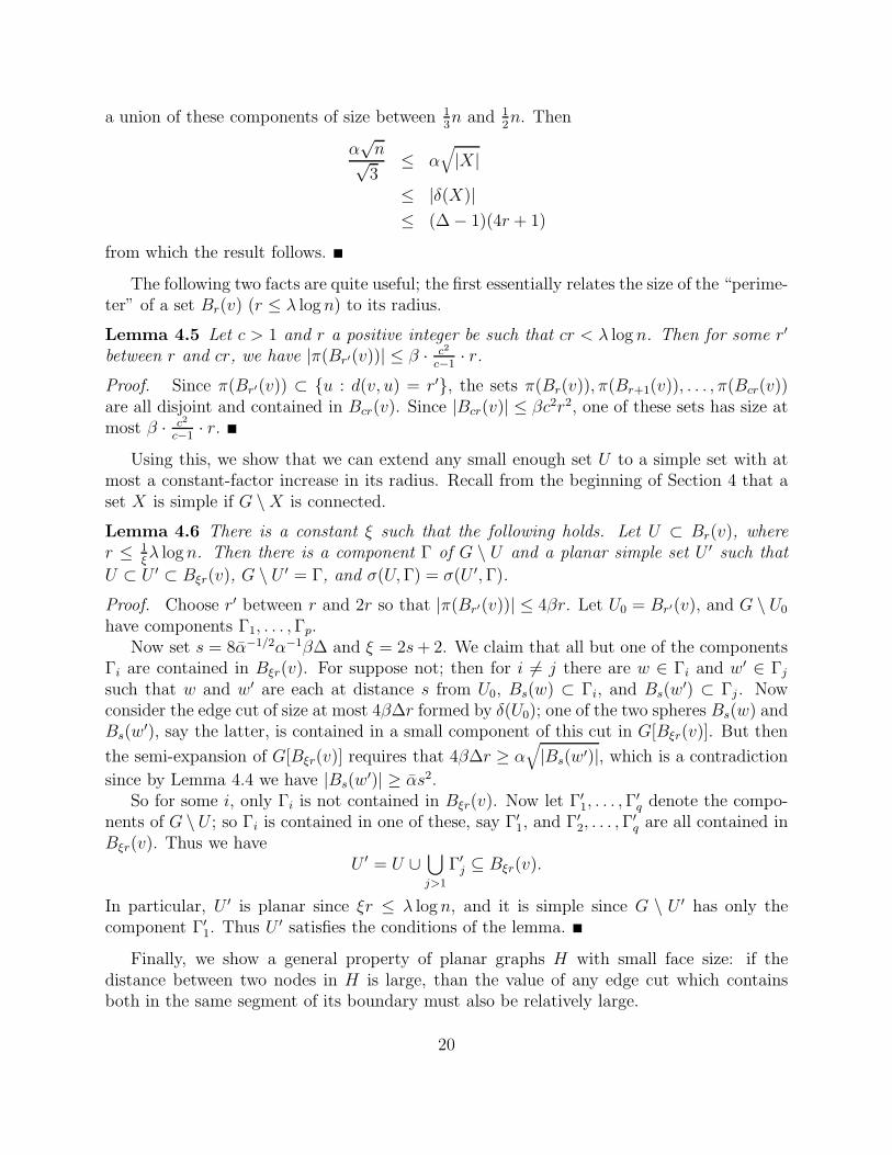
The following two facts are quite useful; the first essentially relates the size of the “perime-ter” of a set Br(v) (r ≤ λ logn) to its radius.

Lemma 4.5 Let c > 1 and r a positive integer be such that cr < λ log n. Then for some r′

between r and cr, we have |π(Br′(v))| ≤ β · c2

c−1· r.

Proof. Since π(Br′(v)) ⊂ u : d(v, u) = r′, the sets π(Br(v)), π(Br+1(v)), . . . , π(Bcr(v))are all disjoint and contained in Bcr(v). Since |Bcr(v)| ≤ βc2r2, one of these sets has size atmost β · c2

c−1· r.

Using this, we show that we can extend any small enough set U to a simple set with atmost a constant-factor increase in its radius. Recall from the beginning of Section 4 that aset X is simple if G \X is connected.

Lemma 4.6 There is a constant ξ such that the following holds. Let U ⊂ Br(v), wherer ≤ 1

ξλ logn. Then there is a component Γ of G \ U and a planar simple set U ′ such that

U ⊂ U ′ ⊂ Bξr(v), G \ U ′ = Γ, and σ(U,Γ) = σ(U ′,Γ).

Proof. Choose r′ between r and 2r so that |π(Br′(v))| ≤ 4βr. Let U0 = Br′(v), and G \ U0

have components Γ1, . . . ,Γp.Now set s = 8α−1/2α−1β∆ and ξ = 2s+ 2. We claim that all but one of the components

Γi are contained in Bξr(v). For suppose not; then for i 6= j there are w ∈ Γi and w′ ∈ Γjsuch that w and w′ are each at distance s from U0, Bs(w) ⊂ Γi, and Bs(w

′) ⊂ Γj . Nowconsider the edge cut of size at most 4β∆r formed by δ(U0); one of the two spheres Bs(w) andBs(w

′), say the latter, is contained in a small component of this cut in G[Bξr(v)]. But then

the semi-expansion of G[Bξr(v)] requires that 4β∆r ≥ α√

|Bs(w′)|, which is a contradiction

since by Lemma 4.4 we have |Bs(w′)| ≥ αs2.

So for some i, only Γi is not contained in Bξr(v). Now let Γ′

1, . . . ,Γ′

q denote the compo-nents of G \U ; so Γi is contained in one of these, say Γ′

1, and Γ′

2, . . . ,Γ′

q are all contained inBξr(v). Thus we have

U ′ = U ∪⋃

j>1

Γ′

j ⊆ Bξr(v).

In particular, U ′ is planar since ξr ≤ λ logn, and it is simple since G \ U ′ has only thecomponent Γ′

1. Thus U ′ satisfies the conditions of the lemma.

Finally, we show a general property of planar graphs H with small face size: if thedistance between two nodes in H is large, than the value of any edge cut which containsboth in the same segment of its boundary must also be relatively large.

20

Lemma 4.7 Let H be a planar graph, with distinguished faces Φ1, . . . ,Φr bounded by cyclesQ1, . . . , Qr respectively. Suppose that all faces other than Φ1, . . . ,Φr are bounded by at mostℓ edges, and for a constant d′ and all i 6= j we have d(Qi, Qj) ≥ d′.

Let U ⊂ V (H) and v, w ∈ σ(U,C) for some component C of G \ U . Then

|δ(U)| ≥ min(ℓ−1d′, ℓ−1d(v, w)).

Proof. Let S = σ(U,C) ⊂ U . In the graph H [U ], S lies on a single facial cycle Q. TraversingQ in a clockwise direction starting at v, we encounter faces R1, . . . , Rp whose boundariescontain vertices both of U and of H \ U .

Suppose that among the Ri there are two distinct large faces Φm and Φm′ . Choosesuch a pair for which Ra = Φm, Rb = Φm′ , and Rc 6∈ Φi for a < c < b. Let P denote thecorresponding maximal subpath of Q whose internal vertices are incident only to faces Rc,for a < c < b. Then among every ℓ consecutive vertices of P , there must be one incidentto an edge in δ(U); since |P | ≥ d′ by the hypotheses of the lemma, this implies the claimedbound.

Otherwise, there is a single large face Φm among the Ri; note that Φm may appearseveral times on the traversal of Q. Now there are two sub-paths of Q from v to w, whichwe denote P0 and P1. Since v, w border the same component of H \ U , the face Φm doesnot appear in a traversal of one of P0 or P1 — suppose it is P0. So as above, among everyℓ consecutive vertices of P0, there must be one incident to an edge in δ(U); and we have|P0| ≥ d(v, w).

4.2 Related Classes of Graphs

In this section, we show a natural construction which produces uniformly densely embeddedgraphs; it is an extension of the definition of geometrically well-formed graphs in our earlierpaper [14]. The material in this section is independent of the rest of the paper.

We wish to define a notion of a surface being locally planar, in the following sense. LetΣ be a compact orientable surface, embedded in R3. For x ∈ Σ, let B′

d(x) denote the set ofall points of Σ whose distance from x (as measured on Σ) is at most d.

Definition 4.8 A set X ⊂ Σ is (γ0, γ1)-flat for some positive constants γ0, γ1, if there is aΣ-disc D such that

(i) X ⊆ D.(ii) For all points x ∈ X and s ≥ 0 such that B′

s(x) ⊂ X, the surface area of B′

s(x) is atleast γ0s

2 and at most γ1s2.

(iii) For all Σ-disc D′ such that D′ ⊆ D, if D′’s boundary has length s, then the surfacearea of D′ is at most γ1s

2.We say that Σ is (r, γ0, γ1)-locally flat if it is orientable, and for all x ∈ Σ the set B′

r(x)is (γ0, γ1)-flat.

21

Of course all these properties hold if Σ, for example, is the unit sphere in R3.Now we say that a graph is locally well-formed if it is drawn on a locally flat surface, and

each face has geometrically about the same (small) size.

Definition 4.9 A graph H drawn on Σ is locally well-formed with constant parameters∆, ℓ, γ0, γ1, ρ0, ρ1 if it has maximum degree ∆ and there is an r > 0 such that

(i) Σ is (r log n, γ0, γ1)-locally flat,(ii) The maximum number of edges on a face in the drawing of H is ℓ, and(iii) for each face Φ of G there is an x ∈ Σ so that B′

ρ0r(x) ⊂ Φ ⊂ B′

ρ1r(x).

We now want to show that every locally well-formed graph is uniformly densely embedded.To show this, the following routine lemma is useful: in Definition 4.1 it is enough to requiresemi-expansion for cuts that produce only two components.

Lemma 4.10 H is an α-semi-expander if and only if the condition of Definition 4.1 holdsfor all sets X for which H [X] and H \X are both connected.

Proof. We proceed by induction on the number of connected components of H [X] and H \X.Assume H [X] is not connected, and let Γ1, . . . ,Γp be components. Then each of the setsΓ1, . . . ,Γp must satisfy Definition 4.1 by the induction hypothesis. From this we get

|δ(X)| =∑

i

|δ(Γi)| ≥ α∑

i

√

|Γi| ≥ α√

|∪iΓi| = α√

|X|.

If H connected but H\X is not, and each connected component has size at most 12|V (H)|,

then the above argument applies to the components ofH\X. Otherwise, apply Definition 4.1to the cut defined by the single large component, both of whose sides are connected.

Proposition 4.11 If G is locally well-formed with parameters ∆, ℓ, γ0, γ1, ρ0, ρ1, then thereare positive constants α and λ such that G is uniformly densely embedded with parametersα, λ, ∆, and ℓ.

Proof. Let G be locally well-formed with the given parameters. Then for any v ∈ V ,if s ≤ ρ−1

1 log n, the set Bs(v) is contained in B′

r logn(v) and hence in a Σ-disc. Now letX ⊂ Bs(v); we wish to show that it satisfies the semi-expansion requirement in G[Bs(v)].By Lemma 4.10, we may assume that both G[X] and G[Bs(v) \ X] are connected. Thusδ(X) lies on a single face of G[X]. Let q = |δ(X)|; then there is a closed curve L on Σ oflength at most ρ1rq that bounds a Σ-disc containing X. Thus, X is contained in a disc ofarea at most γ1ρ

21r

2q2. But each face in G[X] has area at least γ0ρ2r2, so X has at most

γ1ρ21γ

−10 ρ−2

0 q2 faces, and hence at most ℓ times this many vertices.

In a series of papers proving, among other things, that the disjoint paths problem for afixed number of terminal pairs is solvable in polynomial time [27], Robertson and Seymourmake use of another notion of “denseness” of surface embeddings — namely representativity.It turns out that our definition of uniformly densely embedded graphs could also have been

22

expressed in these terms. We say that a closed curve on Σ is null-homotopic if it is homotopicto a point; it is well-known (see e.g. [25]) that a closed curve is null-homotopic if and only ifit is contained in a Σ-disc. Now we say that a drawing of G on Σ is c-representative [25, 26]if any non-null-homotopic closed curve on Σ meets the drawing of G at least c times.

In this terminology, we could have replaced the condition that each G[Br(v)] (r ≤ λ logn)be contained in a Σ-disc by the condition that the drawing of G be Ω(log n)-representative.More precisely,

Proposition 4.12 If G satisfies parts (i) and (iii) of Definition 4.2, and the drawing ofG is (λ logn)-representative, then there is a constant λ′ such that G is uniformly denselyembedded with parameters α, λ′, ∆, and ℓ. Conversely, if G is uniformly densely embeddedwith parameters α, λ, ∆, and ℓ, then there is a constant λ′ such that the drawing of G is(λ′ logn)-representative.

Proof. The converse statement is easier. If G is uniformly densely embedded with parametersα, λ, ∆, and ℓ, then any closed curve R on Σ meeting G at fewer than ℓ−1λ logn verticesmeets it only at vertices contained in Bλ logn(v) for some v ∈ V . Thus R is contained in aΣ-disc and is null-homotopic.

Now suppose G satisfies parts (i) and (iii) of Definition 4.2, and the drawing of G is(λ logn)-representative. We must show that for some λ′, every G[Bλ′ logn(v)] is drawn in aΣ-disc. Choose λ′ < 1

4λ and let U = Bλ′ logn(v) for some v ∈ V . We claim that every simple

cycle of G[U ] is null-homotopic in Σ. For suppose not, and choose the shortest non-null-homotopic cycle Q contained in G[U ]. Say for simplicity that Q contains an even number ofvertices, v0, . . . , vk, . . . , v2k = v0, and let Q0 and Q1 denote the two sub-paths of Q with endsequal to v0 and vk. Now suppose there were some path P in G[U ] with ends equal to v0 andvk of length less than k; then one of Q0 ∪ P or Q1 ∪ P would contain a non-null-homotopicsimple cycle of G[U ] of length less than 2k, contradicting our choice of Q. Thus k ≤ 2λ′ log n,and so |Q| ≤ 4λ′ log n < λ log n. Now since G is strongly embedded, there is a simple closedcurve R on Σ, meeting G at precisely the vertices of Q, that is homotopic to Q in Σ; butsince R meets G fewer than λ logn times, it is null-homotopic in Σ. This contradicts ourassumption that Q is non-null-homotopic.

Thus G[U ] contains only null-homotopic simple cycles. By Theorems (11.2) and (11.10)of [25], this implies that G[U ] is contained in a Σ-disc.

5 Densely Embedded Graphs: The Routing Algorithms

One encounters a number of difficulties in extending the algorithms of Section 3 to denselyembedded graphs in general. Some of these are easily taken care of — for example, we cannotdefine “subsquares” of G anymore; but we can use balls of the form Br(v) instead, and wehave seen above that these behave in much the same way. We similarly may choose a maximalset of mutually distant balls and grow enclosures around them. The major problems are thefollowing. (1) We used the natural crossbars inside a mesh for routing; do these enclosureshave similar crossbars inside them? (2) Where is the high-capacity simulated network N ?

23

To build crossbars inside the enclosures we use the Okamura-Seymour theorem [20],analogously to a construction in our earlier paper [14]. To define the high-capacity simulatednetwork N we want to grow the enclosures out until they touch. However, at this pointtheir boundaries might not be “smooth” enough to allow us to build crossbars inside them;additionally, there is no reason for enclosures that do touch to have Ω(log n) edges in theircommon boundary.

Nevertheless, it is still possible to build a simulated network N , as follows. We growenclosures that have smooth boundaries, and are large enough that they contain large cross-bars, but we keep them mutually distant from one another. Then we define the notionof a Voronoi partition of G to allow us to determine which clusters are “neighbors”; wedefine the simulated network N by putting Ω(log n) parallel edges between neighboring clus-ters (whether or not they have that many edges in the common boundary of their Voronoiregions).

We show that the collection of these parallel edges “represents” the graph G well enoughthat it can be used as the network N . In particular, we need to show that all paths acceptedby the simulated network can be routed in G. For this we make use of a theorem of Schrijver[28]; we show that there exist Ω(log n) paths in G between the neighboring enclosures, suchthat all paths between all pairs are mutually disjoint.

We make no attempt to optimize constants here. Set λ0 = λ, and choose positiveconstants λ1, λ2, . . . so that λj+1 ≪ λj (the exact relationship between these constants iseasy to determine from the analysis below). A connection (si, ti) is short if d(si, ti) ≤ λ2 log nand long otherwise. As before, we handle long and short connections separately; for now weconcentrate on pre-processing the graph as described above for handling long connections.

5.1 Building the Simulated Network

5.1.1 Clusters and Enclosures

We wish to choose a maximal set of mutually distant vertices around which to grow clusters.Let Gr denote the graph obtained from G by joining u and v if d(u, v) ≤ r. We first runLuby’s randomized maximal independent set algorithm [17] in Gλ3 logn.

Let M denote the resulting mis. For any x ∈ V , some vertex within λ5 logn of it willenter M on the first iteration if the largest number chosen in B2λ3 logn(x) is chosen by avertex in Bλ5 logn(x). This happens with constant probability, by Lemma 4.4. Moreover, ifd(x, y) ≥ λ2 logn, then these events are independent for x and y. Thus,

Lemma 5.1 Let x, y ∈ V be such that d(x, y) ≥ λ2 log n. Then with constant probabilitythere are u, v ∈M such that d(x, u) ≤ λ5 logn and d(y, v) ≤ λ5 logn.

Around each v ∈ M we now grow a cluster of radius roughly λ5 log n, and an enclosurearound each cluster, with “smooth” boundaries. We need the following facts. Let H denotean arbitrary graph, and Q a simple cycle of H . For u, v ∈ Q, let dQ(u, v) denote the shortest-path distance from u to v on Q — that is, the length of the shorter of the two u-v paths onQ.

24

λ6 log n paths

λ3 log n

λ4 log n

λ5 log n

cluster

enclosure

crossbar

Figure 2: Building the simulated network

Definition 5.2 We say that Q is ε-smooth if for all u, v ∈ Q we have εdQ(u, v) ≤ d(u, v).

Definition 5.3 If U and W are two subsets of V (H), we say that U is ε′-close to W if foreach u ∈ U there is a w ∈W such that d(u, w) ≤ ε′|W |.

The following fact is quite similar to, but more general than, Theorem 4.4 of our earlierpaper [14]; the proof is very similar as well. In effect, it says that given a cycle Q in aplanar graph H that encloses (in the sense of homotopy) the “hole” formed by some internalface, then for a small ε > 0 we can find a cycle Q′ of no greater length that is ε-close to Q,Ω(ε)-smooth, and also encloses this hole. See Figure 3.

We will use this theorem to smooth out the boundaries of the clusters and the enclosuresaround them.

Theorem 5.4 For each ε > 0 the following holds. Let Σ1 be a compact surface (possiblywith boundary), H a graph embedded on Σ1, and Q a simple cycle of H that is non-null-homotopic on Σ1. Then in polynomial time one can find an ε

1+ε-smooth simple cycle Q′ such

that

25

inner face

outer face

cycle Q

cycle Q′

Figure 3: Smoothing a cycle

(i) |Q′| ≤ |Q|,(ii) Q′ is ε-close to Q, and(iii) Q′ is also non-null-homotopic on Σ1.

Proof. For u, v ∈ Q, let [u, v]Q denote the shorter of the two u-v paths contained in Q (tiesbroken arbitrarily), and let ε = ε

1+ε. If Q is not ε-smooth, then there are u, v ∈ Q such that

εdQ(u, v) > d(u, v). (3)

Moreover, we can efficiently find such a u and v so that there is a shortest u-v path Puv inH that is vertex-disjoint from Q (for example, the pair u, v satisfying (3) for which |Puv| isminimum).

Now one of the two simple cycles [u, v]Q∪Puv and (Q\ [u, v]Q)∪Puv is not null-homotopicon Σ1; and each is shorter than Q. We thus update Q, replacing it with the cycle from amongthese two that is not null-homotopic.

We now iterate this process of “slicing off” parts of Q using short paths through H . Sincethe length of the cycle decreases with each iteration, this process must terminate in a cycleQ′ that is ε-smooth. Moreover, each iteration maintains the invariant that the current cycleis non-null-homotopic on Σ1. Thus, we only have to verify that the final cycle is ε-close toQ.

26

This is clearly true after the first iteration: since |Puv| < εdQ(u, v) < ε|Q|, every vertexon the updated cycle can reach a vertex of Q by a path of length at most ε|Q|. Now, let Qi

denote the cycle obtained after i iterations of slicing off. As long as portions of Q remainon Qi, we say that we are in the “first phase”; other phases will be defined below. In thefirst phase, Qi consists of alternating intervals Qi1, Pi1, Qi2, . . . , Qir, Pir, where Qij ⊂ Q, andthe interval Q′

ij of Q lying between Qij and Qi,j+1 has been sliced off by Pij. We can show

by induction on the number of iterations that |Pij | ≤ ε∣

∣

∣Q′

ij

∣

∣

∣ — as was true after the firstiteration.

This is done by the following case analysis. In the (i+ 1)st iteration, we find a new path;there are three cases to consider.

1. One end of P lies on Qij and the other on Qik, where possibly j = k. Then theproperty clearly continues to hold, since |P | is at most ε times the number of currentcycle vertices cut off, which is in turn at most the number of original vertices of Qbetween the endpoints of P .

2. One end of P lies on Pij and the other on Qik (so Pij is lengthened). Suppose that theamount of original cycle cut off in addition to Q′

ij is equal to x, and the amount of Pijthat is cut off by P is y. Then if Pi+1,j denotes Pij after this iteration, we have

|Pij | ≤ ε∣

∣

∣Q′

ij

∣

∣

∣

|P | ≤ ε(x+ y)

|Pi+1,j | = |Pij | + |P | − y

≤ ε(∣

∣

∣Q′

ij

∣

∣

∣ + x+ y) − y

≤ ε(∣

∣

∣Q′

ij

∣

∣

∣ + x)

3. One end of P lies on Pij and the other lies on Pik (so P glues some of the new pathstogether). There are two subcases.

(i) j = k. Then |Pij | goes down while |Qij | is not affected, so the property still holds.

(ii) j 6= k. Again suppose that the amount of original cycle cut off in addition to Q′

ij

and Q′

ik is equal to x, the amount of Pij cut off by P is y, the amount of Pik cutoff by P is z, and the new interval is denoted Pi+1,j. Then

|Pij| ≤ ε∣

∣

∣Q′

ij

∣

∣

∣

|Pik| ≤ ε|Q′

ik||P | ≤ ε(x+ y + z)

|Pi+1,j| = |Pij | + |P | + |Pik| − y − z

≤ ε(∣

∣

∣Q′

ij

∣

∣

∣ + x+ y + z + |Q′

ik|) − y − z

≤ ε(∣

∣

∣Q′

ij

∣

∣

∣ + x+ |Q′

ik|)

27

If the iterations come to an end before the end of the first phase, then indeed Q′ is ε-closeto Q — any vertex on Pij can reach Q by a path of length at most ε

∣

∣

∣Q′

ij

∣

∣

∣ ≤ ε|Q|. Otherwise,consider the iteration in which the first phase comes to an end. By analogous arguments,we obtain a cycle Q1 such that |Q1| ≤ ε|Q| and every vertex on Q1 can reach Q by a pathof length at most ε|Q|.

Each phase now proceeds exactly like the previous one, except that it begins with a cyclewhose length has been reduced by at least a factor of ε. Thus when the process terminates,all vertices on Q′ will be able to reach Q by a path of length at most

|Q| ·∞∑

i=1

εi = ε|Q|.

Thus Q′ is ε-close to Q.

We use the following procedure to build the clusters and the enclosures around each nodev in M . Let Kv = Bλ5 logn(v).

(i) Choose a radius r between 2λ5 log n and 3λ5 log n so that |π(Br(v))| ≤ 9βλ5 logn. SetCv = Br(v).

(ii) Now extend Cv to a simple set as in Lemma 4.6; since λ3 > 2cλ5, no Cv is grownenough that it overlaps any other by this process.

(iii) We now apply the ε-smoothing algorithm of Theorem 5.4 to the facial cycle Qv ofG[Cv] containing π(Cv). Here Hv = G[Bλ3 logn(v)] \Ko

v plays the role of H , and the cylinderformed by removing the portions of Σ on which G[Ko

v ] and G \ Bλ3 logn(v) are drawn playsthe role of Σ1. Now for a constant ε the resulting cycle Q′

v is ε-smooth in this subgraph Hv

of G, and it is also ε1−ε

-close to Qv. If we choose ε < 118β+1

, then since Qv is initially at least19β|Qv| away from Kv, we know that any path with both ends on Q′

v that passes through Kv

must have length at least 19β|Qv| ≥ 1

9β|Q′

v|. Thus, there are no “short cuts” between verticesof Q′

v that make use of Kv; hence Q′

v is in fact ε-smooth in G.The smooth cycle Q′

v encloses a set S of vertices containing Kv. Update Cv to be thisset S.

We now grow an enclosure Dv ⊃ Cv by the same three-step process, except that we nowuse the constant λ4 in place of λ5, and the set Co

v in place of Kov Thus, we have clusters

of radius ≈ λ5 logn, enclosures of radius ≈ λ4 log n, and they are separated by a mutualdistance of ≈ λ3 log n.

Following the algorithm of Section 3, we now must build crossbar structures in the en-closures to replace the natural crossbars of the mesh. We build crossbars using an extensionof the Okamura–Seymour theorem [20] due to Frank [9], along the same lines as was donein [14]. To be precise,

Definition 5.5 If X ⊂ V , we say a crossbar anchored in X is a set of edge-disjoint paths,each with at least one end in X, such that every pair of paths meets in at least one vertex.

Let σv = π(Cv), and recall that by Q′

v we mean the facial cycle of G[Cv] containing σv.Analogously, let τv = π(Dv), and ϕv the facial cycle of G[Dv] containing τv. We wish to

28

build a crossbar in G[Dv \ Cov ], anchored in σv ∪ τv, of size at least a constant fraction of

|σv ∪ τv|. For a large enough constant κ depending on ε, we choose a set σ′

v of |σv|/κ verticeson σv spaced about κ apart, and a set τ ′v of |τv|/κ on τv spaced about κ apart.

Lemma 5.6 There is a crossbar anchored in σ′

v ∪ τ ′v, such that each vertex of σ′

v ∪ τ ′v is theendpoint of a distinct path of the crossbar.

Proof. Consider the planar graph G[Dv \ Cov ]. This graph has only two large faces — the

outer face bounded by ϕv, and the inner face left by the deletion of Cov . We find a shortest

path P ∗ in the planar dual graph whose endpoints are equal to these two large faces, andwe delete the edges used by this path. Denote the resulting graph by Gv; note that it hasonly a single large face, bounded by a cycle ϕ′

v which contains σ′

v ∪ τ ′v.We claim that the cycle ϕ′

v is ε′-smooth in the graph Gv, where

ε′ = min(1

2ε, (27βℓ)−1).

To see this, suppose that P is a path in Gv with endpoints u, w ∈ ϕ′

v. If u and w both belongto Q′

v, or both belong to ϕv, then this follows from the ε-smoothness of these two cycles inG[Dv \ Co

v ]. If one belongs to each, then |P | ≥ (λ4 − 4λ5) log n, while |ϕ′

v| ≤ 9βℓ(2λ4 + λ5),and again the bound follows. Finally, if both u and w lie on the short dual path P ∗,then in fact |P | ≥ dϕ′

v(u, w), while if exactly one lies on P ∗ then it is easily verified that

|P | ≥ 12εdϕ′

v(u, w).

Write X = σ′

v ∪ τ ′v. Let us assume for simplicity that |X| is odd. Now for u ∈ X, defineu+ to be the vertex on ϕ′

v that is 12κ steps clockwise from u, and write X+ = u+ : u ∈ X.

Now |X ∪X+| is even, so we can pair each u ∈ X ∪ X+ with its unique “antipodal” pointu ∈ X ∪ X+ under the clockwise ordering of ϕ′

v. Note that vertices in X are paired withvertices in X+, and vice versa. We now define a disjoint paths problem in Gv, with the setof terminal pairs Tv equal to (u, u) : u ∈ X. Note that all terminals are at least 1

2κ from

one another on the cycle ϕ′

v.We now want to show that Tv is realizable in Gv. First, say that a cut is non-trivial if

it separates at least one pair of terminals. We are dealing with a disjoint paths problemin a planar graph with all terminals on the outer face. Moreover, every node of Gv not onthe outer face has even degree. In such a case, Frank’s extension of the Okamura-Seymourtheorem [9, 20] says that following strict cut condition is sufficient for the realizability of Tv— every non-trivial cut has more capacity than the number of terminal pairs it separates.

It is enough to consider non-trivial cuts of the form δ(U) with both Gv[U ] and Gv \ Uconnected. For such a set U , there must be two vertices v, w ∈ π(U) such that v, w ∈ ϕ′

v.Suppose that the distance from v to w in Gv is d; then by Lemma 4.7, we have |δ(U)| ≥ ℓ−1d.Since the facial cycle ϕv is ε′-smooth, the number of terminal pairs disconnected by δ(U)is at most 2ε′−1d/κ. Thus taking κ > 2ℓε′−1 ensures that the strict cut condition will besatisfied.

Finally, observe that the edge-disjoint paths in a realization of Tv provide the crossbarrequired by the lemma, since each pair of paths must meet at some vertex of Gv.

29

In the crossbar just constructed, let Y uv denote the path with an endpoint equal to u,

where u ∈ σ′

v ∪ τ ′v.

5.1.2 The simulated network NWe now construct the simulated network; the nodes of this network are the clusters, which werepresent by the vertices in M . We define a neighbor relation on the clusters using the notionof a Voronoi partition; two clusters will be joined by an edge in N if they are neighbors inthis sense.

Let H be a graph and S ⊂ V (H). We fix a lexicographic ordering on the elements ofS. For s ∈ S, let

Us = v ∈ G : ∀s′ ∈ S : d(v, s) ≤ d(v, s′) and ∀s′ s : d(v, s) < d(v, s′).

That is, Us is the set of vertices that are at least as close to s as to any other s′, with tiesbroken based on .

Definition 5.7 The Voronoi partition V(H,S) of H with respect to S is the partition Us :s ∈ S.

The following fact is immediate.

Lemma 5.8 For each s ∈ S, H [Us] is connected.

Proof. Suppose v ∈ Us; we claim that any shortest s-v path P is contained in Us. Forsuppose not, and let v′ ∈ P be the closest vertex to s that lies in Us′ for some s′ 6= s.Then d(s′, v) ≤ d(s, v), and in fact d(s′, v) < d(s, v) if s s′. It follows that v ∈ Us′, acontradiction.

We can now build a graph N (H,S) on the vertices in S, joining two if their Voronoi cellsshare an edge.

Definition 5.9 The neighborhood graph of S in H, denoted N (H,S), is the graph withvertex set S, and an edge (s, s′) iff there is an edge of H with endpoints in Us and Us′.

The simulated graph we use will be the neighborhood graph N (G,M) with every edgegiven capacity ≈ λ6 log n. Let V and N denote V(G,M) and N (G,M) respectively, andN (γ) the graph N in which each edge is given capacity γ.

The following two facts about N are easy to establish. First, by the maximality of M ,we have

Lemma 5.10 For all v ∈M , Uv ⊂ Bλ3 logn(v).

Proof. Suppose u ∈ Uv but d(v, u) > λ3 logn. Then d(v′, u) > λ3 log n for all v′ ∈ M ; thiscontradicts the fact that M is a maximal independent set in Gλ3 logn.

This, along with Lemma 4.4, implies

30

Lemma 5.11 The degree of a vertex in N is at most ∆′ ≤ 16α−1β.

Proof. Let U denote the neighbors of v in N , including v itself. Then by Lemma 5.10,

⋃

u∈U

Uu ⊂ B2λ3 logn(v),

and hence∑

u∈U

|Uu| ≤ 4βλ23 log2 n.

But around each u ∈ U there is a disjoint ball of radius 12λ3 log n, which contains at least

αλ23 log2 n/4 vertices. Thus |U | ≤ 16α−1β.

5.1.3 Inter-Cluster Paths

The goal of this part is, for a constant λ6, to construct λ6 log n disjoint paths between eachpair of enclosures Dv, Dw where (v, w) is an edge in N . This will allow us to convert arouting in the simulated network N (λ6 log n) into actual disjoint paths in G. Recall that theouter facial cycle of G[Dv] is denoted ϕv, and it contains a set τ ′v of vertices evenly spacedat distance κ.

Theorem 5.12 There exist vertex-disjoint paths in G, each with ends in sets τ ′v and oth-erwise disjoint from all Dv, such that for (v, w) ∈ N , there are at least λ6 log n such pathswith one end in τ ′v and the other in τ ′w.

Proof. The proof is based on the following theorem of Schrijver [28]. Let Σ1 be a surface(possibly with boundary), H a graph embedded on Σ1, and Ai : i = 1, . . . , k a set ofdisjoint curves on Σ1 each of which is either closed or anchored at vertices of H on theboundary of Σ1. The problem is to find vertex-disjoint paths and cycles P i in G so thatP i is homotopic to Ai for each i.

Call a collection of curves R on Σ1 essential if it consists either of a single closed curvethat is not null-homotopic, or it is a finite union of curves each with endpoints on theboundary of Σ1. Schrijver [28] proves that such vertex-disjoint paths and cycles exist if foreach essential collection of curves R, there are curves Bi, where Bi is homotopic to Ai,such that R intersects the drawing of H more than it intersects the curves Bi. (The mainresult of [28] is in fact a necessary and sufficient condition; this weaker statement suffices forour purposes. Additionally, [28] is stated for the special case of surfaces without boundary,but the extension we use here follows immediately from [28].)

Say that a curve is G-normal if it meets the drawing of G only at vertices, and define itsG-length to be the number of times it meets the drawing. For each v, v′ that are neighborsin N , we draw a G-normal arc Avv′ on Σ with endpoints v and v′. We can ensure that allthese arcs are disjoint, since each Uv is connected, and for each (v, v′) ∈ E(N ), there is atleast one edge of G with endpoints in Uv and Uv′ . Choose a small constant λ6 ≤ |τ ′v|/∆′ (say,less than 1

8α2α∆′−2∆−2λ−1

3 λ24; the reason for this will become clear below). Now suppose we

31

pull out these crossings

R

Auu′

Dv1

Dv2

Dv3

Figure 4: Pulling out a crossing

have in fact λ6 logn copies of each Avv′ , all running “parallel” to one another. By pushingthem apart appropriately, we can assume that each arc runs through a different vertex in τ ′vand τ ′v′ . Let Auu′ denote the G-normal arc that runs through u ∈ τ ′v and u′ ∈ τ ′v′ .

Define G′ to be the graph obtained by deleting Dov for each v ∈ M . We now cut Σ

along the facial cycles ϕv to obtain Σ′, a surface with boundary. Note that G′ is properlyembedded on Σ′. The theorem is now a consequence of the following claim.

Claim 5.13 There exist vertex-disjoint paths Puu′ in G′ such that Puu′ is homotopic to Auu′.

Proof. If curves R and R′ are homotopic, we write R ∼ R′. We extend this notation tofinite collections of curves R, R′

in the obvious way. Following notation of Schrijver [28],the number of crossings of R0 and R1 is denoted cr(R0,R1), and we define

mincr(R0,R1) = mincr(R′

0,R′

1) : R0 ∼ R′

0,R1 ∼ R′

1.

By the theorem of Schrijver [28] given above, the desired paths exist if for each essentialcollection of curves R on Σ′, one has

cr(R, G′) >∑

(u,u′)

mincr(R, Auu′). (4)

Note that in verifying this inequality, we may assume R is G′-normal, and that R has noself-crossings.

32

For a collection of curves R, define its index to be

cr(R, G′) −∑

(u,u′)

mincr(R, Auu′).

So it is enough to consider collections of curves R whose index is minimum in their homotopyclass, and to show that such R in fact have positive index.

Set r = 12∆−1αα1/2λ4 logn. We claim that no G-normal closed curve of G-length less than

2r can enclose a set of the form Dv. For if it did, then Dv could be disconnected by an edgecut of size less than αα1/2λ4 log n, which is not possible since |Dv| ≥ αλ2

4 log2 n. From thisit follows that any G′-normal closed curve of G′-length less than 2r must be null-homotopicin Σ′.

Note that we can view the expression cr(R, G′) − ∑

(u,u′) cr(R, Auu′) as a sum over the

finitely many arc-components of R; if the value of this expression is not positive, we show howmodify the curves Auu′ so that it increases. We do this by considering each arc-componentof R in turn. Let R denote a single arc-component of R; we consider two cases, based onthe G′-length of R.

Case 1. cr(R, G′) ≤ r. Then R must have both endpoints on the same facial cycle(it is too short to touch two such cycles, and if it were a closed curve it would have to benull-homotopic, by the above argument.) But then it is easy to produce arcs A′

uu for whichcr(R, G′) >

∑

(u,u′) cr(R, A′

uu′) since ϕv is ε-smooth.Case 2. cr(R, G′) > r. Again, we just have to exhibit arcs A′

uu′ ∼ Auu′ lying on Σ′ sothat

cr(R, G′) >∑

(u,u′)

cr(R, A′

uu′), (5)

without increasing the number of crossings of these arcs with the other components of R. Ifthe set Auu′ satisfies (5), we are done; otherwise, we show how to modify this set of arcsso that it does. See Figure 4.

If the set Auu′ does not satisfy Inequality (5), then there is some interval R′ of R ofG′-length r for which (5) is violated. Let us consider such an R′.

Observe that each arc Auu′ has G′-length at most 2λ3 logn, and hence at most ∆′2λ6 log nof these arcs can meet R′, since at most ∆′2 pairs of clusters have at least one end closeenough to R′. Now suppose the total number of crossings of these arcs with R′ exceeds

(2λ3 logn)(∆′2λ6 log n)

r< cr(R′, G).

Then some arc Auu′ meets R′ more than 2λ3 log n/r times, and hence the interval of Auu′between some pair of consecutive crossings with R′ has G′-length less than r.

Suppose that this pair of consecutive crossings occurs at vertices w and w′. Let R′′ denotethe G′-normal curve formed from this interval of Auu′ and the portion of R′ between w andw′. R′′ has G′-length less than 2r, and so it must be null-homotopic by the argument givenabove.

33

Now, since R has minimum index over all curves in its homotopy class, the portion ofAuu′ between w and w′ meets G′ at least as many times as the portion of R′ between w andw′. We can therefore modify Auu′ so that it runs along R′ for this interval. This does notincrease the G′-length of Auu′; and it decreases the number of crossings of R — as well asR (since it has no self-crossings) — with Auu′ .

Thus this process terminates; when it does, we have a set of arcs A′

uu′ for whichInequality 5 holds.

Let us denote one such path with ends u and u′ by Zuu′. Moreover, we have u ∈ τ ′vand u′ ∈ τ ′v′ , and they are ends of paths Y u

v and Y u′

v′ respectively. Denote by Zuu′ theconcatenation of the three paths Y u

v , Zuu′, and Y u′

v′ .

5.2 The On-Line Algorithm

With the simulated network N in place, the routing algorithms themselves are essentiallythe same as those for the mesh; here we just describe what must be modified.

First of all, the analogue of Lemma 3.10 is the following.

Lemma 5.14 Let r ≤ λ1 logn, U ⊂ Br(v) for some v ∈ V , and T ′ a set of terminal pairsin U . Then the maximum size of a subset of T ′ that is realizable in B8ξ2r(v) is within aconstant factor of the maximum size of a subset of T ′ that is realizable in G.

Proof. First choose a radius r′ between 2r and 3r for which |π(Br(v)| ≤ 9βr′. Thenconstruct a simple set extension of Br′(v) as in Lemma 4.6; and ε-smooth its outer facialcycle to obtain a set U ′ ⊃ U contained in B4ξr(v). Let U ′′ ⊂ B8ξ2r denote a simple setextension of B8ξr(v), as in Lemma 4.6. For a constant κ′, we can pick a set S of vertices onthe outer facial cycle of U ′ spaced κ′ apart, and use Frank’s theorem [9] as in Lemma 5.6to construct a set of edge-disjoint paths connecting “antipodal” pairs in S, such that allpaths stay within U ′′ \ U ′. Note that we must take care to ensure that the parity conditionis met, since the outer facial cycle of U ′′ can contain odd-degree vertices. To do this weremove sub-paths of this cycle between consecutive pairs of the (necessarily even number of)odd-degree vertices; U ′′ is large enough that the strict cut condition will remain satisfied.

Consider the set of paths in a realization of a maximum-size subset of T ′ in G. Of thepaths that meet π(U ′), we can select a constant fraction of paths such that the the pairs offirst and last intersections with π(U ′) can be connected along the outer facial cycle of U ′ todifferent vertices in S. We can then use the crossbar of the previous paragraph to connect allof these pairs together; the resulting paths are within a constant fraction of the maximumnumber achievable in G, and they do not leave U ′′.

The algorithm for short connections is now as follows. We run a randomized version ofLuby’s algorithm, this time in Gλ1 logn. Let M ′ denote the resulting mis. With constantprobability, both ends of a short connection are within 1

16ξ2λ1 log n of the same v ∈ M ′, as

in Lemmas 3.11 and 5.1. We now let Uv denote Bλ1 logn/16ξ2(v) and only route connectionsboth of whose ends lie in the same Uv. To route such connections, we run the algorithm of

34

Proposition 3.9 in each B 12λ1 logn(v); by Lemma 5.14, this is within O(logn) of optimal in

each Uv.For long connections, we run the same simulation as in the case of the mesh, this time

in the graph N (λ6 logn). The analogue of Lemma 3.6 holds exactly as before, as doesLemma 3.7 — making use of the paths Zuu′, since all such paths incident to the sameenclosure must cross. Finally, the analogue of Lemma 3.8 is the following.

Lemma 5.15 There is a constant γ such that for any realizable subset T ′ of T , ψ(T ′) canbe routed in N (γ log n).

Proof. Set γ = 9β(∆′3λ5 + λ3). For each si-ti path P in the optimal routing, construct thefollowing path for (ui, vi) in N — when P crosses from Uw into Uw′, add an edge from wto w′. Now consider how many paths in our constructed routing use the edge (w,w′). Eachsuch corresponds to a path in the original routing that used an edge in δ(Uw,Uw′). We can’tbound the size of this set directly, since it could be quite “meandering.” But consider thefollowing argument. δ(Uw,Uw′) ⊂ B2λ3 logn(x) for some vertex x ∈ G; thus there is some rbetween 2λ3 logn and 3λ3 log n so that |π(Br(x))| ≤ 9βλ3 log n. So at most this many pathswith both ends more than r away from x can use edge in δ(Uw,Uw′). But closer than this,there are at most ∆′3 clusters, each of which is the origin of at most 9βλ5 logn paths.

Thus the optimum in G is bounded by the fractional optimum in N (γ log n), which is atmost a constant factor more than the fractional optimum in N (λ6 logn), which is at most anO(logn) factor more than the number of pairs routed by the on-line algorithm in G. Thuswe have

Theorem 5.16 The on-line algorithm is O(logn)-competitive in any uniformly densely em-bedded Eulerian graph G.

5.3 The Off-Line Algorithm

The off-line algorithm too is essentially the same, now working with the larger simulatednetwork N ′(λ6 log n). The only change required is in the proof of Lemma 3.15. Here, we areno longer able to talk about “overfull rectangles”; however, we can define a round cut to bea set of the form Br(w) ∩Cv. Since a given u ∈ Cv is only contained in O(r2) round cuts ofradius r, the following lemma establishes that round cuts can be used instead of rectanglesin the analogue of Lemma 3.15 for densely embedded graphs.

Lemma 5.17 Let G′

v denote G[Cv] with an additional vertex zv joined by an edge to eachvertex in σ′

v. Then there is a constant ξ1 such that for every U ⊂ G′

v not containing zv, thereis a round cut R ⊇ U satisfying |δ(R)| ≤ ξ1|δ(U)|.

Proof. Set ξ′1 = κ1 + α−1/2α−1 and ξ1 = 4∆ξ′1(β+ ε−1). Let U ⊂ G′

v be a set not containingzv, and write p = |δ(U)|; we construct a round cut R containing U for which |δ(R)| ≤ ξ1p.

35

Now if we contract G′

v \ U to a single vertex, we obtain a planar graph with maximumface size κ1 (as opposed to ℓ; this is due to the large spacing of the vertices of σ′

v). So byLemma 4.7, the maximum distance between two points on π(U) is at most κ1p.

Next we claim that every vertex in U must be within distance α−1/2α−1p of π(U). Thereason for this is analogous to the proof of Lemma 4.6 — if not, then U would contain aball of more than this radius, which would contain more than α−1p2 vertices; a contradictionsince |δ(U)| = p.

Thus for any u ∈ π(U), we have U ⊂ Br(u), where

r = (κ1 + α−1/2α−1)p = ξ′1p.

Now by Lemma 4.5, there is an r′ between r and 2r such that

|δ(Br′(u))| ≤ 4β∆ξ′1p.

Now let R ⊃ U denote the round cut Br′(u)∩Cv. Every edge of δ(R) is an edge of eitherδ(Br′(u)) or of δ(Cv ∩ R). The former quantity was just shown to be at most 4β∆ξ′1p. Tobound the latter quantity, note that any two vertices in π(Cv ∩ R) are at most 2r′ ≤ 4ξ′1papart; since the facial cycle containing π(Cv) is ε-smooth, this means that π(Cv∩R) containsat most 4ε−1ξ′1p vertices, and hence

|δ(Cv ∩R)| ≤ 4∆ε−1ξ′1p.

The claim now follows since

|δ(R)| ≤ 4∆ξ′1(β + ε−1)p = ξ1p.

Thus we have

Theorem 5.18 There is a randomized (off-line) mdpp algorithm in uniformly densely em-bedded Eulerian graphs that produces a constant-factor approximation with high probability.

6 Extensions

6.1 Durations and Profits

In the on-line algorithm we assume that (i) all connections have infinite duration, and (ii) allconnections have the same “value” (i.e. our objective function could have been a weightedsum of the set of pairs we accept, rather than an unweighted sum). However, there aregeneral transformation techniques due to Awerbuch et. al. [5] that allow us to convert ourresults to on-line algorithms that can handle connections of limited duration and variablevalue, at the cost of additional logarithmic terms in the competitive ratio. Specifically, wepay O(logT ) and O(logP ), where T and P are the ratios between the largest and smallestdurations and values respectively.

36

6.2 Graphs with an Exceptional Face

In this section, we sketch the extension of our algorithms to densely embedded, nearly-Eulerian graphs. Recall from Definition 4.3 that such a graph satisfies the properties of auniformly densely embedded Eulerian graph, except that it is allowed to contain an “excep-tional” face Φ∗, with facial cycle Q∗ that may have length greater than ℓ and may containvertices not of even degree.

For the remainder of this section, let G denote a densely embedded, nearly-Euleriangraph with parameters α, λ, ∆, and ℓ. For simplicity, we assume that the facial cycle Q∗ issufficiently large that it is not contained in any set Bλ logn(v); it is not difficult to removethis assumption.

The changes required in the algorithm come from the fact that there can now be a G-normal curve joining two distant vertices in G that intersects G relatively few times — thisis because it can pass through the large face Φ∗. This has consequences in the proofs ofLemma 5.6 (and its relatives) and Claim 5.13. However, by requiring the outer cycles ofclusters and enclosures to satisfy a more restrictive notion of ε-smoothness, these facts willfollow as before.

We define our more restrictive type of ε-smoothness as follows. Let G/Q∗ denote thegraph G with a single additional node q∗ joined by length-0 edges to each vertex of the longfacial cycle Q∗. Then a small cut passing through two distant vertices, as described in theprevious paragraph, does correspond to a short path in G/Q∗ — it simply makes use of theadditional node q∗. Now it is straightforward to show that we need only require the outercycles of the clusters and enclosures to be ε-smooth in the graph G/Q∗; and this can beaccomplished by running the ε-smoothing algorithm in this graph instead of in G.

This introduces a further difficulty, however. Say that we have just smoothed some cycleQ, obtaining a cycle Q′. While Q′ will be ε-close to the original cycle Q in G/Q∗, there isno reason why this means it will be ε-close in G.

To handle this, we strengthen the statement of Theorem 5.4, as follows. For a vertex u,define the u-restricted distance du(v, w) between two vertices v and w to be the minimumlength of a v-w path avoiding u. From the proof of Theorem 5.4, one sees that we canalways find a short path from the smooth cycle Q′ back to the original cycle Q that avoidsany prescribed vertex; i.e.Q′ is ε-close toQ with respect to any u-restricted distance function.In particular, Q′ is ε-close to Q in G/Q∗ with respect to the q∗-restricted distance function;that is, Q′ is ε-close to Q in the original graph G.

Thus, we can obtain clusters and enclosures with boundaries which are ε-smooth inG/Q∗,and which are not far from the original boundaries in G. The sets τ ′v will now consist ofevenly spaced vertices only on the part of an enclosure’s outer facial cycle that does not lieon Φ∗. The proof of Lemma 5.6 now follows exactly as before. When we use Schrijver’stheorem to construct inter-cluster paths, we also cut the surface Σ along the long facial cycleQ∗ so as to remove Φ∗ from the surface. Now an essential curve can be anchored on theboundary of Φ∗ as well as on the boundary of an enclosure; but this poses no problem sincethe enclosure boundaries are ε-smooth in G/Q∗.

Once the simulated network N has been set up, the on-line and off-line algorithms work

37

exactly as before. (In particular, Lemma 5.17 follows without modification, since the largeface Φ∗ is incorporated into the hypotheses of Lemma 4.7.) Thus we have,

Theorem 6.1 There is an O(logn)-competitive on-line mdpp approximation in any denselyembedded nearly-Eulerian graph.

Theorem 6.2 There is a randomized (off-line) mdpp algorithm in any densely embeddednearly-Eulerian graph that produces a constant-factor approximation with high probability.

Acknowledgements

We thank Yuval Rabani for his contribution to this work. In particular, he suggested thegeneral approach of performing randomized rounding on graphs with low-capacity edges andthrowing out parts of the routing on which the capacity constraints become violated. Thanksalso to Baruch Awerbuch, Michel Goemans, David Karger, Tom Leighton, and Lex Schrijverfor their comments on these problems.

References

[1] A. Aggarwal, A. Bar-Noy, D. Coppersmith, R. Ramaswami, B. Schieber, M. Sudan,“Efficient routing and scheduling algorithms for optical networks,” Proc. 5th ACM-SIAMSODA, 1994, pp. 412–423.

[2] J. Aspnes, Y. Azar, A. Fiat, S. Plotkin and O. Waarts, “On-line Load Balancing withApplications to Machine Scheduling and Virtual Circuit Routing” Proc 25th ACM STOC,1993.

[3] Y. Aumann, Y. Rabani, “Improved bounds for all-optical routing,” Proc. 6th ACM-SIAMSODA, 1995, pp. 567–576.

[4] B. Awerbuch, Y. Azar, S. Plotkin, “Throughput-Competitive Online Routing,” Proc.34th IEEE FOCS, 1993, pp. 32–40.

[5] B. Awerbuch, Y. Bartal, A. Fiat, A. Rosen, “Competitive non-preemptive call control,”Proc. 5th ACM-SIAM SODA.

[6] B. Awerbuch, R. Gawlick, F.T. Leighton, Y. Rabani, “On-line admission control andcircuit routing for high performance computing and communication,” Proc. 35th IEEEFOCS, 1994, pp. 412–423.

[7] A. Broder, A. Frieze, S. Suen, E. Upfal, “Optimal construction of edge-disjoint paths inrandom graphs,” Proc. 5th ACM-SIAM SODA, 1994, pp. 603–612.

[8] A. Broder, A. Frieze, E. Upfal, “Existence and construction of edge-disjoint paths onexpander graphs,” SIAM J. Computing, 23(1994), pp. 976–989.

38

[9] A. Frank, “Edge-disjoint paths in planar graphs,” J. Comb. Theory Ser. B, 39(1985), pp.164–178.

[10] A. Frank, “Packing paths, cuts, and circuits — a survey,” in Paths, Flows, and VLSI-Layout, B. Korte, L. Lovasz, H.J. Promel, A. Schrijver, Eds., Berlin: Springer-Verlag,1990. pp. 49–100.

[11] N. Garg, V. Vazirani, M. Yannakakis, “Primal-dual approximation algorithms for in-tegral flow and multicut in trees, with applications to matching and set cover,” Proc.ICALP, 1993, pp. 64–75.

[12] R.M. Karp, “Reducibility among combinatorial problems,” Complexity of ComputerComputations, R.E. Miller, J.W. Thatcher, Eds., New York: Plenum Press, 1972. pp.85–103.

[13] J. Kleinberg, S. Rao, E. Tardos, “Routing with low congestion in densely embeddedgraphs,” in preparation.

[14] J. Kleinberg, E. Tardos, “Approximations for the disjoint paths problem in high-diameter planar networks,” Proc. 27th ACM STOC, 1995.

[15] M.E. Kramer, J. van Leeuwen, “The complexity of wire routing and finding the mini-mum area layouts for arbitrary VLSI circuits,” Advances in Computing Research 2: VLSITheory, F.P. Preparata, Ed., London: JAI Press, 1984. pp. 129–146.

[16] R. Lipton, R. Tarjan, “A separator theorem for planar graphs,” SIAM J. Applied Math.36(1979), pp. 177–189.

[17] M. Luby, “A simple parallel algorithm for the maximal independent set problem,” SIAMJ. Computing, 15(1986), pp. 1036–1053.

[18] W. Massey, Algebraic Topology: An Introduction, New York: Springer-Verlag, 1967.

[19] M. Middendorf, F. Pfeiffer, “On the complexity of the disjoint paths problem,” Combi-natorica, 13(1993). pp. 97–107.

[20] H. Okamura, P. Seymour, “Multicommodity flows in planar graphs,” J. Comb. TheorySer. B, 31(1981), pp. 75–81.

[21] D. Peleg, E. Upfal, “Disjoint paths on expander graphs,” Combinatorica, 9(1989), pp.289–313.

[22] P. Raghavan, “Probabilistic construction of deterministic algorithms: approximatingpacking integer programs,” J. Computer and System Sciences, 37(1988), pp. 130–143.

[23] P. Raghavan, C.D. Thompson, “Randomized rounding: a technique for provably goodalgorithms and algorithmic proofs,” Combinatorica, 7(1987), pp. 365–374.

39

[24] P. Raghavan, E. Upfal, “Efficient all-optical routing,” Proc. 26th ACM STOC, 1994,pp. 134–143.

[25] N. Robertson, P.D. Seymour, “Graph Minors VII. Disjoint paths on a surface,” J. Com-binatorial Theory Ser. B, 45(1988), pp. 212–254.

[26] N. Robertson, P.D. Seymour, “Graph Minors XI. Circuits on a surface,” J. Combina-torial Theory Ser. B, 60(1994), pp. 72–106.

[27] N. Robertson, P.D. Seymour, “Graph Minors XIII. The disjoint paths problem,”J. Combinatorial Theory Ser. B, 63(1995), pp. 65–110.

[28] A. Schrijver, “Disjoint circuits of prescribed homotopies in a graph on a compact sur-face,” J. Combinatorial Theory Ser. B, 51(1991), pp. 127–159.

[29] D. Sleator, R. Tarjan, “Amortized efficiency of list update and paging rules,” Comm.ACM, 23(1985), pp. 202–208.

[30] D. Wagner, K. Weihe, “A linear time algorithm for multicommodity flow in planargraphs,” Proc. First European Symposium on Algorithms, 1993, pp. 384–395.

40