Dispatching Rules for Production Scheduling:a Hyper-heuristic Landscape Analysis

Gabriela Ochoa, Jose Antonio Vazquez-Rodrıguez, Sanja Petrovic and Edmund Burke

Abstract— Hyper-heuristics or “heuristics to chose heuristics”are an emergent search methodology that seeks to automate theprocess of selecting or combining simpler heuristics in order tosolve hard computational search problems. The distinguishingfeature of hyper-heuristics, as compared to other heuristicsearch algorithms, is that they operate on a search space ofheuristics rather than directly on the search space of solutionsto the underlying problem. Therefore, a detailed understandingof the properties of these heuristic search spaces is of utmostimportance for understanding the behaviour and improvingthe design of hyper-heuristic methods. Heuristics search spacescan be studied using the metaphor of fitness landscapes.This paper formalises the notion of hyper-heuristic landscapesand performs a landscape analysis of the heuristic searchspace induced by a dispatching-rule-based hyper-heuristic forproduction scheduling. The studied hyper-heuristic spaces arefound to be “easy” to search. They also exhibit some specialfeatures such as positional bias and neutrality. It is argued thatsearch methods that exploit these features may enhance theperformance of hyper-heuristics.

I. INTRODUCTION

Despite the success of evolutionary algorithms and otherheuristic search methods in solving real-world computationalsearch problems, there are still some difficulties for easilyapplying them to newly encountered problems, or evennew instances of known problems. These difficulties arisemainly from the significant range of parameter or algorithmchoices involved when using this type of approaches, andthe lack of guidance as to how to proceed for selectingthem. Another drawback of these techniques is that state-of-the-art approaches for real-world problems tend to representbespoke problem-specific methods which are expensive todevelop and maintain. Hyper-heuristics or “heuristics tochose heuristics”[3] are an emergent search methodologythat seeks to automate the process of selecting or combiningsimpler heuristics in order to solve hard computational searchproblems. The main motivation behind hyper-heuristics is toraise the level of generality in which search methodologiescan operate. A hyper-heuristic approach consists of a high-level general strategy that coordinates the efforts of a setof low-level (usually problem specific) heuristics to solvethe underlying problem. The distinguishing feature of hyper-heuristics, as compared to other heuristic search algorithms,is that they operate on a search space of heuristics rather thandirectly on the search space of solutions to the underlying

G. Ochoa, J.A. Vazquez-Rodrıguez, S. Petrovic, and E. Burke are withthe Automated Scheduling, optimisAtion and Planning Research Group,School of Computer Science and Information Technology, University ofNottingham, Jubilee Campus, Wollaton Road, Nottingham, NG8 1BB, UK,(email: gxo, jav, sxp, ekb @cs.nott.ac.uk).

problem. In consequence, a detailed understanding of theproperties of these heuristics search spaces is of utmost im-portance for understanding the behaviour and improving thedesign of hyper-heuristic methods. Heuristic search spacescan be studied using the metaphor of fitness landscapes, inwhich the search space is regarded as a spatial structurewhere each point (solution) has a height (objective functionvalue) forming a landscape surface. Both local and globalfeatures of search landscapes can be estimated by statisticalmethods (see [18] for an introduction to landscape analysis).

In the domain of Job-Shop Scheduling, Fisher and Thomp-son [9], [10] hypothesised that combining scheduling rules(also known as priority or dispatching rules) would be supe-rior than any of the rules taken separately. This pioneeringwork, well ahead its time, proposed a method of combiningscheduling rules using “probabilistic learning”. Notice that inthe early 60s, meta-heuristic and local search techniques werestill not mature. However, the proposed learning approachresembles a stochastic local search algorithm (indeed aestimation of distribution algorithm) operating in the spaceof scheduling rule sequences. The main conclusions fromthis study are the following: “(1) an unbiased random com-bination of scheduling rules is better than any of them takenseparately; (2) learning is possible” [10]. The ideas by Fisherand Thompson [9], [10] were independently rediscovered andenhanced, several times, 30 years later [7], [8], [20], [21],when modern meta-heuristics were already widely knownand used. Therefore, the authors had the appropriate con-ceptual and algorithmic tools (also the computer power) topropose and conduct search within a heuristic search space.More recent studies using dispatching rules as low-levelheuristics in hyper-heuristic approaches are those describedin [22], [23].

This paper conducts a landscape analysis of the heuristicsearch space induced by the dispatching-rule-based hyper-heuristic for production scheduling presented in [22], [23].The underlying problem studied is the hybrid flowshopscheduling problem. Dispatching rules are among the mostfrequently applied heuristic in production scheduling, dueto their ease of implementation and low time complexity.Whenever a machine is available, a dispatching rule inspectsthe waiting jobs and selects the job with the highest priorityto be processed next. Dispatching rules differ from each otherin the way they calculate priorities. A candidate solution inthe studied heuristic space is, therefore, given by a sequence(list) of dispatching rules. Each rule in this list is successivelyused to select one operation (or group of operations) to beassigned next to its required machine.

The paper is structured as follows. Section II describes theunderlying problem domain and the hyper-heuristic approachunder study. Thereafter, section III describes the notion offitness landscapes and the metrics employed in our analysis;it also presents a formal definition of hyper-heuristics land-scapes. Section IV describes our methodology, whilst sectionV reports our results regarding performance and landscapeanalysis. Finally, section VI, summarises and discusses ourmain findings.

II. A HYPER-HEURISTIC APPROACH TO THE HYBRIDFLOW SHOP PROBLEM

The hybrid flow shop scheduling problem (HFS) consistsof assigning n jobs into m processing stages; all jobs areprocessed in the same order: stage 1, stage 2, . . . , until stagem. At least one of the stages has two or more identicalmachines working in parallel. No job can be processed onmore than one machine at a time, and no machine can processmore than one job at a time. Several objective functions havebeen proposed for the HFS. Let cj and dj be the completiontime of job j, i.e. the time when it exists the shop, and itsdue date, respectively. We considered two objective functionsfor measuring the quality of the schedules: (1) the makespandenoted Cmax and defined as Cmax = maxj(cj) and (2) thetotal weighted tardiness, denoted sumWT and defined assumWT =

∑nj=1 wj ·max{0, cj−dj}, where wj is a weight

associated with job j. The interested reader is referred to[24] for a more detailed description of HFS formulation andobjective functions, and a review of approaches developedfor the problem.

The HFS is very common in real world manufacturing.It is encountered in the electronics industry, ceramic tilesmanufacturing, cardboard box manufacturing and many otherindustries. HFS scheduling is an NP-Hard problem, evenwhen there are just two processing stages with one of themhaving a single machine, and one having parallel machines[12]. The relevance and complexity of the HFS problem havemotivated the investigation of a variety of methods including:exact methods [5], [25], heuristics [19], [6], meta-heuristics[11], [1], and more recently hyper-heuristics [22], [23]

Since there are n jobs to be processed in m stages, thenumber of decisions to be made is N = n ×m. Therefore,decisions 1 to n correspond to the scheduling of operationsin the first stage of the shop, from n to 2n to jobs in thesecond stage of the shop and so on. Let us consider the taskof deciding the order in which n jobs have to be scheduledon a machine for a given stage. Fulfilling this task requiresdeciding which job is to be processed 1st, which job is tobe processed 2nd and so on. Let d1 be the first of thesedecisions, d2 the 2nd, and so on. The task requires, then,n − 1 decisions (no decision is required when there is onejob left). Let D be the set of all decisions defining a problemand N = |D|.

Definition 1: D = {d1, . . . , dN} is the set of decisionsdefining a problem, where di is the ith decision to be made.

Let us give an illustrative example: suppose 7 jobs are tobe scheduled, i.e. n = 7, and for simplicity let us assume a

single stage (m = 1). Thus, D = {d1, . . . , d6}. Let us denoteby pj the processing time of job j. The processing times ofthe jobs are p = {10, 20, 30, 40, 50, 60, 70}. Let H be therepository of low level heuristics, i.e. the set of heuristicswhich are available to make the decisions in D. Suppose Hcontains two elements; h1: assign next the not-yet scheduledjob with the shortest processing time; and h2: assign nextthe not-yet scheduled job with the longest processing time.A feasible solution to the given 7 jobs scheduling problemcan be obtained as follows.

Step 1: assign a low level heuristic from H to each of thedecisions in D. Let ai ∈ H be the heuristic assigned to di.Step 2: call successively a1, a2, . . . , a6 to select the 1st,2nd, . . . , 6th job to be processed.Step 3: assign last the remaining operation and calculate thestarting and completion times of jobs.

In this way a search mechanism, such as a genetic algorithm(GA), may be used to find a sequence of heuristics inthe form A = [a1, a2, . . . , a6] which is translated into asolution as explained above. Suppose that the followingassignment of heuristics is generated by the GA, A′ =[h1, h1, h1, h2, h2, h2]. Using the described procedure, thistranslates into the sequence of jobs 1, 2, 3, 7, 6, 5, 4. A sched-ule is obtained by calculating the starting and completiontime of each job. The task of the GA algorithm or any otherheuristic search mechanism, then, would be to decide whichelement of H to assign to each ai. In consequence, the sizeof the heuristic search space (for each stage) is in this case26, as there are two possible heuristics for each of the 6assignments.

As discussed in [23] the scheduling decisions can begrouped into decision blocks. In the above example, anassignment of heuristics with the form A = [a1, a2, a3] mayalso represent a feasible solution if it is translated into aschedule as follows.

Step 1: assign a1 to d1 and d2; assign a2 to d3 and d4; assigna3 to d5 and d6.Steps 2 and 3: as above.

In this way, A′ = [h1, h2, h1] translates into 1, 2, 7, 6, 3, 4, 5.In this second type of assignment (A) the decisions weregrouped in 3 blocks, having two operations each (the lastblock has 3 operations).

Notice that in this case, the size of the search spacedecreases to 23 as we have now only 3 assignments to make.More generally, the size of the heuristic space will be |H||A|,where H denotes the repository of heuristics, and A, thesequence of assignments.

III. FITNESS LANDSCAPES

The notion of fitness landscapes [18] was introduced todescribe the dynamics of adaptation in nature [26]. Sincethen, it has become a powerful metaphor in evolutionarytheory. The fitness landscape metaphor can be used for search

in general. Given a search problem, the set of possiblesolutions can be coded using strings of fixed length fromsome finite alphabet. This encoding generates a representa-tion space, which is a high dimensional space of all possiblestrings of a given length. There is also a neighborhoodrelation that defines which points in the representation spaceare connected. This relation depends on the specific searchoperator or combination of operators, used to search thespace. Finally, there is a fitness function that assigns a fitnessvalue to each possible string or point in the space.

More formally [15], a fitness landscape (S, f, d) of aproblem instance of a given combinatorial optimization prob-lem consists of a set of candidate solutions S, a fitness (orobjective) function f : S 7→ R, which assigns a real-valuedfitness to each solution in S, and a distance metric d thatdefines the spatial structure of the landscape. This distanceis related to the neighborhood relation described above.

A. Fitness distance correlation analysis

The most commonly used measure to estimate the globalstructure of fitness landscapes is the fitness distance cor-relation (FDC) coefficient, proposed by Jones and Forrest[13]. It is used as a measure for problem difficulty in geneticalgorithms. Given a set of points x1, x2, . . . .xm and if fitnessvalues, the FDC coefficient % is defined as:

%(f, dopt) =Cov(f, dopt)σ(f)σ(dopt)

(1)

where Cov(., .) denotes the covariance of two random vari-ables and σ(.) the standard deviation. The FDC determineshow closely related are the fitness of a set of points andtheir distances to the nearest optimum in the search space(denoted by dopt). If fitness increases when the distance tothe optimum becomes smaller, then the search is expectedto be easy, since the optimum can gradually be approachedvia fitter individuals. A value of % = −1.0 (% = 1.0) formaximisation (minimisation) problems indicates a perfectcorrelation between fitness and distance to the optimum, andthus predicts an easy search. On the other hand, a valueof % = 1.0 (% = −1.0), means that with increasing fitnessthe distance to the optimum increases too, which indicates adeceptive and difficult problem. As suggested in [13], a valueof fdc ≤ −0.5 (fdc ≥ 0.5) for maximisation (minimisation)problems indicates an easy problem.

Often, a fitness distance plot is made to gain insight intothe structure of the landscape, in addition to (or instead of)calculating the correlation coefficient [15]. This is done byplotting the fitness of points in the search space against theirdistance to an optimum or best-known solution. This typeof analysis, often called fitness distance analysis, can beused to investigate not only the correlation between arbitrarypoints in the search space, but also the distribution of localoptima within the search space. An interesting propertyof fitness landscapes, which has been observed in manydifferent studies [2], [14], [15], [17], is that on average,local optima are very much closer to the optimum than

are randomly chosen points, and closer to each other thanrandom points would be. In other words, the local optima arenot randomly distributed, rather they tend to be clustered in a“central massif” (or “big valley” if we are minimising). Thisglobal structure has been observed in the abstract NK familyof landscapes [14], and in many combinatorial optimisationproblems, such as the traveling salesman problem [2], graphbipartitioning [15], and flowshop scheduling [17].

B. Hyper-heuristic Landscapes

Our hyper-heuristic approach (described in section II),deals with two search spaces: (1) the search space ofheuristics (HS), and (2) the search space of solutions tothe problem at hand (PS). However, we have a singlelandscape, as the objective function value of a point in theheuristic search space, can only be known after calculatingthe objective value of the corresponding search point in thesolution space. Figure 1 illustrates the two search spacesdiscussed and the two mappings involved, namely, g froma heuristic list to its corresponding problem solution, andf from the solution to the objective value. More formally,the objective function of a sequence of heuristics A inthe heuristic space HS is given by the composition of gand f , namely, f(g(A)) : HS 7→ R. The hyper-heuristiclandscape is, therefore, defined as the triplet (HS, f(g), V ),where the first two components are defined as above, andV represents the neighbourhood produced by the minimalpossible move operator on the heuristic search space (referredto as 1 − move). That is, the operator that substitutes oneheuristic in the sequence by another (randomly selected)heuristic from the repository of low-level heuristics.

IV. EXPERIMENTAL SETTINGS

Two groups of experiments were conducted, the first groupcompares the performance attained by different problem rep-resentations (search spaces), defined by grouping decisionsin different block sizes. A direct encoding of the problembased on permutations (i.e. a permutation search space), is aalso explored.

Four instances of the hybrid flowhsop problem wererandomly generated with different numbers of jobs, n ∈{50, 100}, and stages, m ∈ {5, 20}. The processing timeswere generated randomly using a discrete uniform distribu-tion in the [10,100] interval. Note that the processing time ofjobs in different stages may differ. The number of machinesper stage were either 4 or 5, both with equal probability.

For each problem instance, several ways of groupingdecisions were studied. The representation that considerseach decision individually, was always considered. In thisrepresentation there are n blocks of size 1 per stage; sincethere are m stages, there is a total of n × m decisionblocks. Let us consider for example the case of 50 jobs,the distribution of decision blocks in stages is as follows:

b1, . . . , b50︸ ︷︷ ︸stage 1

, b51, . . . , b100︸ ︷︷ ︸stage 2

, . . . , b50(m−1)+1, . . . , b50m︸ ︷︷ ︸stage m

.

h1 h2 h3 … hn

Objective Function(makespan,

completion times,max tardiness, etc)

Heuristic space:sequence of dispatchingrules

Problem space: flow shopschedules

Real numbers: objectivefunction value of theschedule

g f

Fig. 1. Hyper-heuristic mapping process from a sequence of heuristics to its fitness value. Two mappings are involved: g : HS 7→ PS, and f : PS 7→ R.

For n = 50, decisions were also grouped into 10 and30 decision blocks per stage. When 10 blocks per stage areconsidered, each block contains 5 decisions, and when 30blocks are considered, the first 20 blocks contain 2 decisionseach whilst the last 10 one decision each. Similarly, for n =100, blocks of size 25, 50, and 100 were used.

A repository of 13 dispatching-rules were consideredas low-level heuristics to be potentially assigned to eachdecision. These heuristics works as follows: whenever amachine is idle, select the job not yet scheduled and readyfor processing (released from the previous stage) that bestsatisfies a certain criterion and assign it to the idle machine.The following rules were considered: minimum release time,shortest processing time, longest processing time, less workremaining, more work remaining, earliest due date, latestdue date, weighed shortest processing time, weighted longestprocessing time, lowest weighted work remaining, highestweighted work remaining, lowest weighted due date andhighest weighted due date.

A standard GA with elitism was employed as the high-level strategy searching on the different heuristic spaces, andthe permutation space. The crossover operator implementedselects two chromosomes as parents, and sets any gene ciof the new chromosome with a probability α from the fittestparent and 1-α from the other. The mutation operator selects(n × m) × β random genes and substitutes them with adifferent randomly selected dispatching rule. Parameter β(0 < β < 1) controls the strength of mutation. The GAcontrol parameters that produced the best results after an sta-tistical tuning process [23] were used, namely: a populationsize of 100, and binary tournament selection with elitism.The algorithm selects the genetic operators independently toproduce offspring; crossover with a probability of 0.9, andmutation with 0.1. The α and β parameters described aboveare set to 0.5 and 0.05, respectively. The stopping conditionwas set to 10 000 solution evaluations, and for each instanceand representation 30 GA runs were conducted.

V. RESULTS

Table I, summarises the average performance obtained af-ter 30 GA runs for each representation and objective functionon the four instances studied. The best obtained results foreach instance and objective function are highlighted in boldfont. Notice that the hyper-heuristic representation clearlyoutperformed the permutation representation in all cases,and the advantage of the heuristic representation is morenoticeable for the sumWT objective function. Note also thatgrouping several decisions into blocks, that is, having shorterhyper-heuristic representations, seems to be favourable whenconsidering a fixed computational effort. This was alreadyobserved in [23], where it was also found that consideringtoo many or too few decision blocks per stage yieldedcomparably poor results. A large number of decision blocksper stage implies a larger search space, whereas very fewdecision blocks have very limited expression power, this mayexplain the observed behaviour.

A. Landscape analysis

It is clear from the results discussed above that the hyper-heuristic search spaces offer an advantage when solving HFSproblems. With the aim of gaining a better understanding ofthe structure of such search spaces, this section reports ourstatistical landscape analysis.

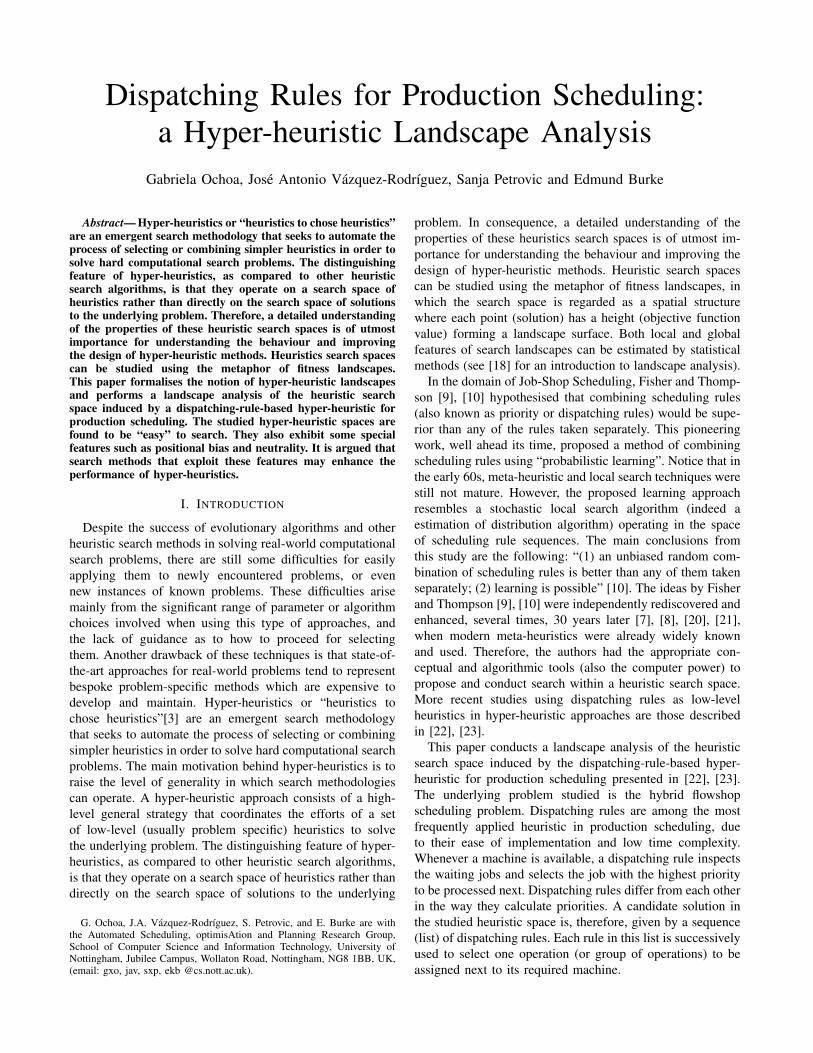
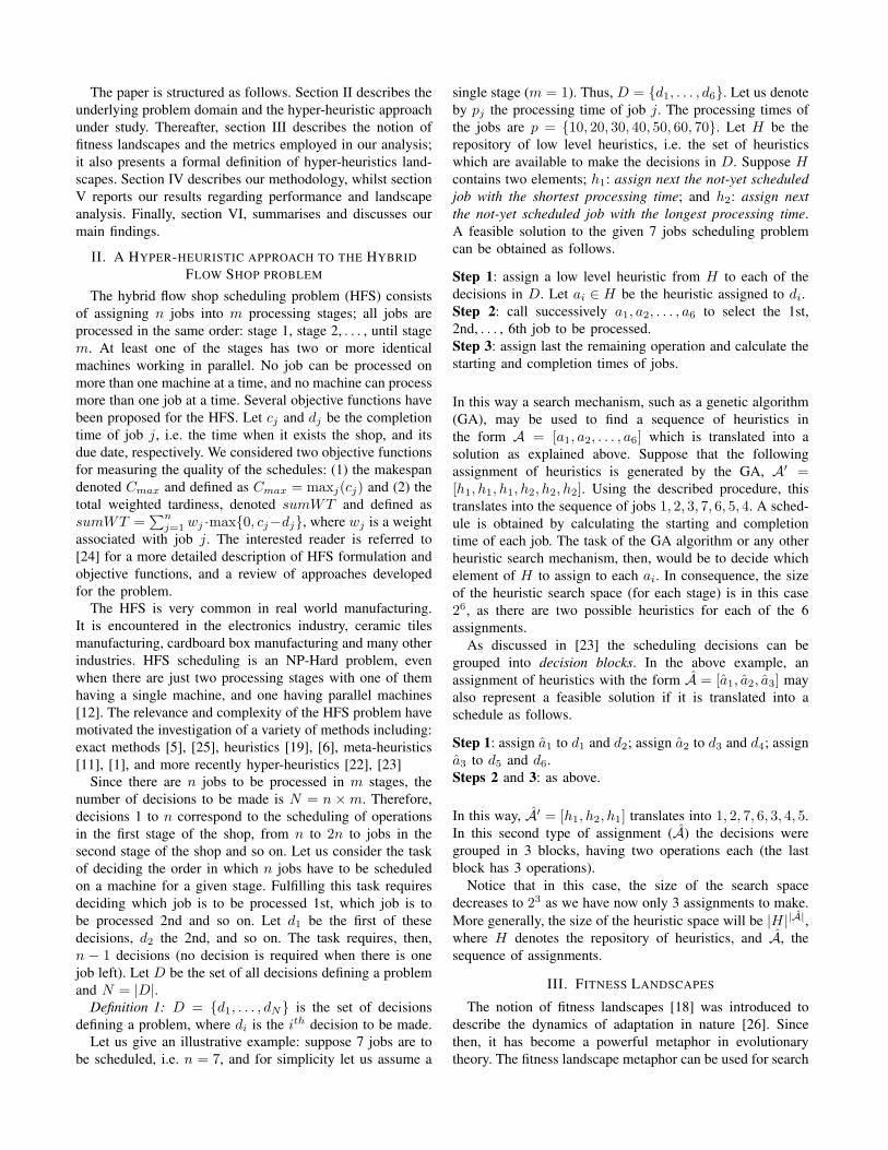
1) Heuristic space vs. permutation space: distribution ofobjective values: First, we compared the distribution ofobjective values, for both Cmax and sumWT , of a set of10 000 randomly generated solutions on both the permutationand hyper-heuristic search spaces. The permutation spacewas sampled by generating random permutations which weredecoded as schedules by assigning jobs in their order ofappearance into the first machine to become available. Theschedules were generated in such a way that there are noidle time windows on any machine that are large enough toprocess a job without delaying the completion time of anyother job. Therefore, only active schedules were generated,

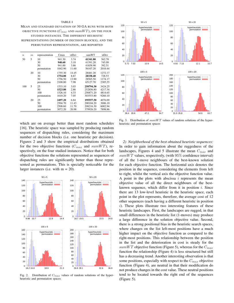
TABLE IMEAN AND STANDARD DEVIATION OF 30 GA RUNS WITH BOTH

OBJECTIVE FUNCTIONS (Cmax AND sumWT ), ON THE FOUR

STUDIED INSTANCES. THE DIFFERENT HEURISTIC

REPRESENTATIONS (NUMBER OF DECISION BLOCKS), AND THE

PERMUTATION REPRESENTATION, ARE REPORTED

.n m representation Cmax stDev sumWT stDev

50 5 10 941.30 3.74 41341.80 562.7830 940.60 3.10 41391.20 745.0950 941.00 3.86 41858.90 392.51permutation 1042.90 11.60 56107.20 2010.44

20 10 1755.30 14.45 28481.20 1272.1730 1754.00 8.87 28338.40 728.5350 1756.50 13.90 28565.50 1174.17permutation 2100.80 7.98 65127.70 2305.55

100 5 25 1533.10 3.03 250794.30 3424.2550 1523.80 2.86 252856.80 4217.34100 1526.10 4.33 256871.20 4814.65permutation 1610.20 7.05 303553.80 9260.10

20 25 2497.20 6.84 195557.50 4076.0950 2504.70 11.43 200104.20 3686.10100 2508.60 11.70 208216.30 6002.94permutation 3072.20 20.98 379926.20 7898.86

which are on average better than most random schedules[16]. The heuristic space was sampled by producing randomsequences of dispatching rules, considering the maximumnumber of decision blocks (i.e. one heuristic per decision).Figures 2 and 3 show the empirical distributions obtainedfor the two objective functions (Cmax and sumWT ), re-spectively, on the four studied instances. Notice that for bothobjective functions the solutions represented as sequences ofdispatching rules are significantly better than those repre-sented as permutations. This is specially noticeable for thelarger instances (i.e. with m = 20).

0

20

40

60

80

100

120

140

9.98 10.7 12.8 14.4

50 x 5

hyperheuristicpermutation

0

20

40

60

80

100

120

140

18.7 19.5 22.5 24.9

50 x 20

hyperheuristicpermutation

0

20

40

60

80

100

120

140

160

16.2 16.8 18.9 21.3

100 x 5

hyperheuristicpermutation

0

20

40

60

80

100

120

140

160

180

200

26.8 28.1 32.6 36.9

100 x 20

hyperheuristicpermutation

Fig. 2. Distribution of Cmax values of random solutions of the hyper-heuristic and permutation spaces

0

20

40

60

80

100

120

5.72 7.53 10.9 14.5

50 x 5

hyperheuristicpermutation

0

20

40

60

80

100

120

4.93 7.13 12.1 15.7

50 x 20

hyperheuristicpermutation

0

20

40

60

80

100

120

36.4 39.8 47.2 54.7

100 x 5

hyperheuristicpermutation

0

20

40

60

80

100

120

140

160

180

200

31.9 35.8 54.6 63.7

100 x 20

hyperheuristicpermutation

Fig. 3. Distribution of sumWT values of random solutions of the hyper-heuristic and permutation spaces

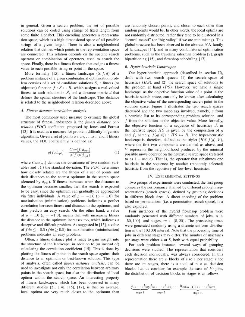
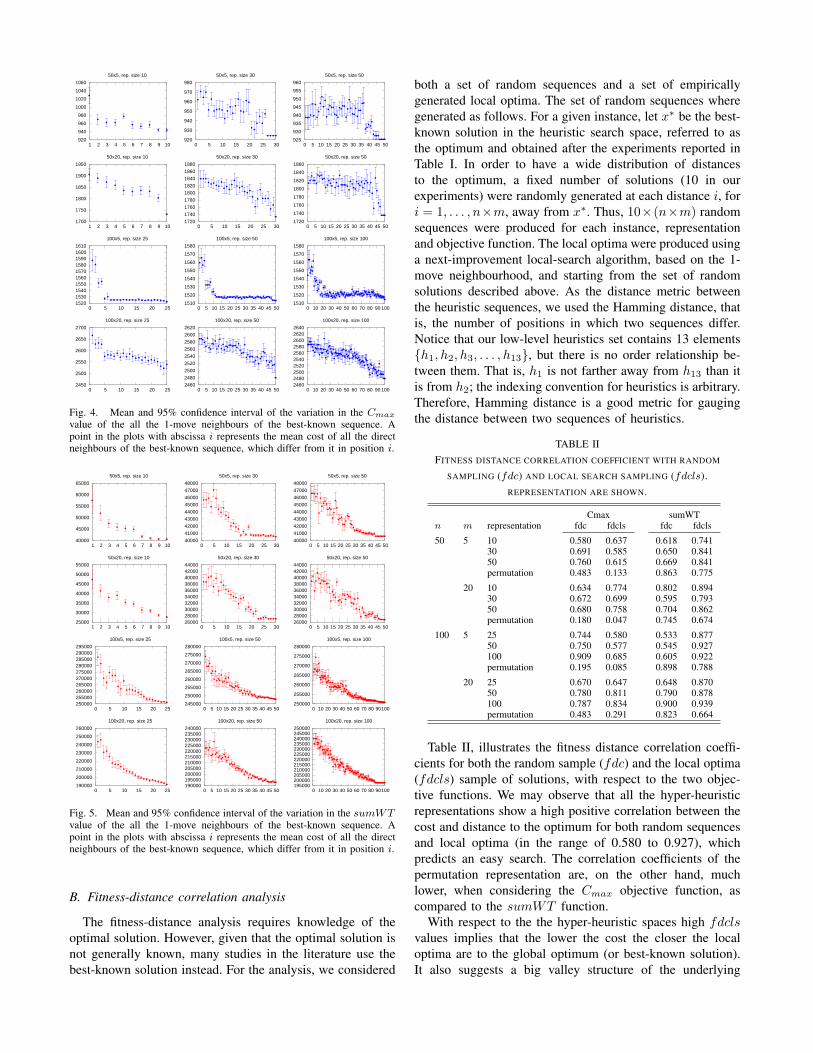
2) Neighborhood of the best obtained heuristic sequences:In order to gain information about the ruggedness of thelandscapes, Figures 4 and 5 illustrate the mean Cmax andsumWT values, respectively, (with 95% confidence interval)of all the 1-move neighbours of the best-known solutionfor each objective function. The horizontal axis denotes theposition in the sequence, considering the elements from leftto right, whilst the vertical axis the objective function value.A point in the plots with abscissa i represents the meanobjective value of all the direct neighbours of the best-known sequence, which differ from it in position i. Sincethere are 13 low-level heuristic in the heuristic space, eachpoint in the plot represents, therefore, the average cost of 12other sequences (each having a different heuristic in positioni). These plots illustrate two interesting features of theseheuristic landscapes. First, the landscapes are rugged, in thatsmall differences in the heuristic list (1-moves) may producea large difference in the solution objective value. Second,there is a strong positional bias in the heuristic search spaces,where changes on the list left-most positions have a muchhigher impact on the objective function as compared to theright-most positions. This relationship between the positionin the list and the deterioration in cost is steady for thesumWT objective function (Figure 5), whereas for the Cmax

function the relationship (Figure 4) is less structured but stillhas a decreasing trend. Another interesting observation is thatsome positions, especially with respect to the Cmax objectivefunction (Figure 4), are neutral in that their modification donot produce changes in the cost value. These neutral positionstend to be located towards the right end of the sequences(Figure 5).

920

940

960

980

1000

1020

1040

1060

1 2 3 4 5 6 7 8 9 10

50x5, rep. size 10

1700

1750

1800

1850

1900

1950

1 2 3 4 5 6 7 8 9 10

50x20, rep. size 10

1520 1530 1540 1550 1560 1570 1580 1590 1600 1610

0 5 10 15 20 25

100x5, rep. size 25

2450

2500

2550

2600

2650

2700

0 5 10 15 20 25

100x20, rep. size 25

920

930

940

950

960

970

980

0 5 10 15 20 25 30

50x5, rep. size 30

1720

1740

1760

1780

1800

1820

1840

1860

1880

0 5 10 15 20 25 30

50x20, rep. size 30

1510

1520

1530

1540

1550

1560

1570

1580

0 5 10 15 20 25 30 35 40 45 50

100x5, rep. size 50

2460

2480

2500

2520

2540

2560

2580

2600

2620

0 5 10 15 20 25 30 35 40 45 50

100x20, rep. size 50

925

930

935

940

945

950

955

960

0 5 10 15 20 25 30 35 40 45 50

50x5, rep. size 50

1720

1740

1760

1780

1800

1820

1840

1860

0 5 10 15 20 25 30 35 40 45 50

50x20, rep. size 50

1510

1520

1530

1540

1550

1560

1570

1580

0 10 20 30 40 50 60 70 80 90 100

100x5, rep. size 100

2460 2480 2500 2520 2540 2560 2580 2600 2620 2640

0 10 20 30 40 50 60 70 80 90 100

100x20, rep. size 100

Fig. 4. Mean and 95% confidence interval of the variation in the Cmax

value of the all the 1-move neighbours of the best-known sequence. Apoint in the plots with abscissa i represents the mean cost of all the directneighbours of the best-known sequence, which differ from it in position i.

40000

45000

50000

55000

60000

65000

1 2 3 4 5 6 7 8 9 10

50x5, rep. size 10

25000

30000

35000

40000

45000

50000

55000

1 2 3 4 5 6 7 8 9 10

50x20, rep. size 10

250000 255000 260000 265000 270000 275000 280000 285000 290000 295000

0 5 10 15 20 25

100x5, rep. size 25

190000

200000

210000

220000

230000

240000

250000

260000

0 5 10 15 20 25

100x20, rep. size 25

40000

41000

42000

43000

44000

45000

46000

47000

48000

0 5 10 15 20 25 30

50x5, rep. size 30

26000 28000 30000 32000 34000 36000 38000 40000 42000 44000

0 5 10 15 20 25 30

50x20, rep. size 30

245000

250000

255000

260000

265000

270000

275000

280000

0 5 10 15 20 25 30 35 40 45 50

100x5, rep. size 50

190000 195000 200000 205000 210000 215000 220000 225000 230000 235000 240000

0 5 10 15 20 25 30 35 40 45 50

100x20, rep. size 50

40000

41000

42000

43000

44000

45000

46000

47000

48000

0 5 10 15 20 25 30 35 40 45 50

50x5, rep. size 50

26000 28000 30000 32000 34000 36000 38000 40000 42000 44000

0 5 10 15 20 25 30 35 40 45 50

50x20, rep. size 50

250000

255000

260000

265000

270000

275000

280000

0 10 20 30 40 50 60 70 80 90 100

100x5, rep. size 100

195000 200000 205000 210000 215000 220000 225000 230000 235000 240000 245000 250000

0 10 20 30 40 50 60 70 80 90 100

100x20, rep. size 100

Fig. 5. Mean and 95% confidence interval of the variation in the sumWTvalue of the all the 1-move neighbours of the best-known sequence. Apoint in the plots with abscissa i represents the mean cost of all the directneighbours of the best-known sequence, which differ from it in position i.

B. Fitness-distance correlation analysis

The fitness-distance analysis requires knowledge of theoptimal solution. However, given that the optimal solution isnot generally known, many studies in the literature use thebest-known solution instead. For the analysis, we considered

both a set of random sequences and a set of empiricallygenerated local optima. The set of random sequences wheregenerated as follows. For a given instance, let x∗ be the best-known solution in the heuristic search space, referred to asthe optimum and obtained after the experiments reported inTable I. In order to have a wide distribution of distancesto the optimum, a fixed number of solutions (10 in ourexperiments) were randomly generated at each distance i, fori = 1, . . . , n×m, away from x∗. Thus, 10×(n×m) randomsequences were produced for each instance, representationand objective function. The local optima were produced usinga next-improvement local-search algorithm, based on the 1-move neighbourhood, and starting from the set of randomsolutions described above. As the distance metric betweenthe heuristic sequences, we used the Hamming distance, thatis, the number of positions in which two sequences differ.Notice that our low-level heuristics set contains 13 elements{h1, h2, h3, . . . , h13}, but there is no order relationship be-tween them. That is, h1 is not farther away from h13 than itis from h2; the indexing convention for heuristics is arbitrary.Therefore, Hamming distance is a good metric for gaugingthe distance between two sequences of heuristics.

TABLE IIFITNESS DISTANCE CORRELATION COEFFICIENT WITH RANDOM

SAMPLING (fdc) AND LOCAL SEARCH SAMPLING (fdcls).REPRESENTATION ARE SHOWN.

Cmax sumWTn m representation fdc fdcls fdc fdcls

50 5 10 0.580 0.637 0.618 0.74130 0.691 0.585 0.650 0.84150 0.760 0.615 0.669 0.841permutation 0.483 0.133 0.863 0.775

20 10 0.634 0.774 0.802 0.89430 0.672 0.699 0.595 0.79350 0.680 0.758 0.704 0.862permutation 0.180 0.047 0.745 0.674

100 5 25 0.744 0.580 0.533 0.87750 0.750 0.577 0.545 0.927100 0.909 0.685 0.605 0.922permutation 0.195 0.085 0.898 0.788

20 25 0.670 0.647 0.648 0.87050 0.780 0.811 0.790 0.878100 0.787 0.834 0.900 0.939permutation 0.483 0.291 0.823 0.664

Table II, illustrates the fitness distance correlation coeffi-cients for both the random sample (fdc) and the local optima(fdcls) sample of solutions, with respect to the two objec-tive functions. We may observe that all the hyper-heuristicrepresentations show a high positive correlation between thecost and distance to the optimum for both random sequencesand local optima (in the range of 0.580 to 0.927), whichpredicts an easy search. The correlation coefficients of thepermutation representation are, on the other hand, muchlower, when considering the Cmax objective function, ascompared to the sumWT function.

With respect to the the hyper-heuristic spaces high fdclsvalues implies that the lower the cost the closer the localoptima are to the global optimum (or best-known solution).It also suggests a big valley structure of the underlying

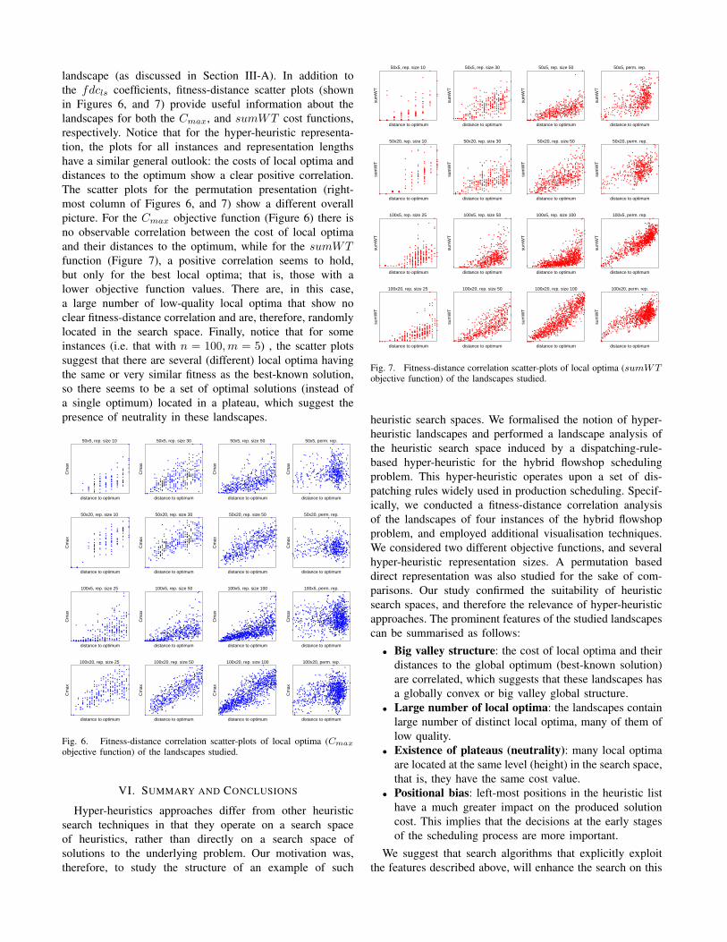
landscape (as discussed in Section III-A). In addition tothe fdcls coefficients, fitness-distance scatter plots (shownin Figures 6, and 7) provide useful information about thelandscapes for both the Cmax, and sumWT cost functions,respectively. Notice that for the hyper-heuristic representa-tion, the plots for all instances and representation lengthshave a similar general outlook: the costs of local optima anddistances to the optimum show a clear positive correlation.The scatter plots for the permutation presentation (right-most column of Figures 6, and 7) show a different overallpicture. For the Cmax objective function (Figure 6) there isno observable correlation between the cost of local optimaand their distances to the optimum, while for the sumWTfunction (Figure 7), a positive correlation seems to hold,but only for the best local optima; that is, those with alower objective function values. There are, in this case,a large number of low-quality local optima that show noclear fitness-distance correlation and are, therefore, randomlylocated in the search space. Finally, notice that for someinstances (i.e. that with n = 100,m = 5) , the scatter plotssuggest that there are several (different) local optima havingthe same or very similar fitness as the best-known solution,so there seems to be a set of optimal solutions (instead ofa single optimum) located in a plateau, which suggest thepresence of neutrality in these landscapes.

Cm

ax

distance to optimum

50x5, rep. size 10

Cm

ax

distance to optimum

50x20, rep. size 10

Cm

ax

distance to optimum

100x5, rep. size 25

Cm

ax

distance to optimum

100x20, rep. size 25

Cm

ax

distance to optimum

50x5, rep. size 30

Cm

ax

distance to optimum

50x20, rep. size 30

Cm

ax

distance to optimum

100x5, rep. size 50

Cm

ax

distance to optimum

100x20, rep. size 50

Cm

ax

distance to optimum

50x5, rep. size 50

Cm

ax

distance to optimum

50x20, rep. size 50

Cm

ax

distance to optimum

100x5, rep. size 100

Cm

ax

distance to optimum

100x20, rep. size 100

Cm

ax

distance to optimum

50x5, perm. rep.

Cm

ax

distance to optimum

50x20, perm. rep.

Cm

ax

distance to optimum

100x5, perm. rep.

Cm

ax

distance to optimum

100x20, perm. rep.

Fig. 6. Fitness-distance correlation scatter-plots of local optima (Cmax

objective function) of the landscapes studied.

VI. SUMMARY AND CONCLUSIONS

Hyper-heuristics approaches differ from other heuristicsearch techniques in that they operate on a search spaceof heuristics, rather than directly on a search space ofsolutions to the underlying problem. Our motivation was,therefore, to study the structure of an example of such

sum

WT

distance to optimum

50x5, rep. size 10

sum

WT

distance to optimum

50x20, rep. size 10

sum

WT

distance to optimum

100x5, rep. size 25

sum

WT

distance to optimum

100x20, rep. size 25

sum

WT

distance to optimum

50x5, rep. size 30

sum

WT

distance to optimum

50x20, rep. size 30

sum

WT

distance to optimum

100x5, rep. size 50

sum

WT

distance to optimum

100x20, rep. size 50

sum

WT

distance to optimum

50x5, rep. size 50

sum

WT

distance to optimum

50x20, rep. size 50

sum

WT

distance to optimum

100x5, rep. size 100

sum

WT

distance to optimum

100x20, rep. size 100

sum

WT

distance to optimum

50x5, perm. rep.

sum

WT

distance to optimum

50x20, perm. rep.

sum

WT

distance to optimum

100x5, perm. rep.

sum

WT

distance to optimum

100x20, perm. rep.

Fig. 7. Fitness-distance correlation scatter-plots of local optima (sumWTobjective function) of the landscapes studied.

heuristic search spaces. We formalised the notion of hyper-heuristic landscapes and performed a landscape analysis ofthe heuristic search space induced by a dispatching-rule-based hyper-heuristic for the hybrid flowshop schedulingproblem. This hyper-heuristic operates upon a set of dis-patching rules widely used in production scheduling. Specif-ically, we conducted a fitness-distance correlation analysisof the landscapes of four instances of the hybrid flowshopproblem, and employed additional visualisation techniques.We considered two different objective functions, and severalhyper-heuristic representation sizes. A permutation baseddirect representation was also studied for the sake of com-parisons. Our study confirmed the suitability of heuristicsearch spaces, and therefore the relevance of hyper-heuristicapproaches. The prominent features of the studied landscapescan be summarised as follows:• Big valley structure: the cost of local optima and their

distances to the global optimum (best-known solution)are correlated, which suggests that these landscapes hasa globally convex or big valley global structure.

• Large number of local optima: the landscapes containlarge number of distinct local optima, many of them oflow quality.

• Existence of plateaus (neutrality): many local optimaare located at the same level (height) in the search space,that is, they have the same cost value.

• Positional bias: left-most positions in the heuristic listhave a much greater impact on the produced solutioncost. This implies that the decisions at the early stagesof the scheduling process are more important.

We suggest that search algorithms that explicitly exploitthe features described above, will enhance the search on this

type of heuristic search space. These performance predictionsshould be tested in future work. Moreover, similar and moreadvanced landscape analysis techniques should be conductedon both larger set of instances and types of productionscheduling problems.

REFERENCES

[1] A. Allahverdi and F. S. Al-Anzi. Scheduling multi-stage parallel-processor services to minimize average response time. Journal of theOperational Research Society, 57:101–110, 2006.

[2] K. D. Boese, A. B. Kahng, and S. Muddu. A new adaptive multi-starttechnique for combinatorial global optimizations. Operations ResearchLetters, 16:101–113, 1994.

[3] E. K. Burke, E. Hart, G. Kendall, J. Newall, P. Ross, and S. Schu-lenburg. Hyper-heuristics: An emerging direction in modern searchtechnology. In F. Glover and G. Kochenberger, editors, Handbook ofMetaheuristics, pages 457–474. Kluwer, 2003.

[4] E. K. Burke, B. McCollum, A. Meisels, S. Petrovic, and R. Qu.A graph-based hyper-heuristic for educational timetabling problems.European Journal of Operational Research, 176:177–192, 2007.

[5] J. Carlier and E. Neron. An exact method for solving the multi-processor flow-shop. RAIRO Research Operationale, 34:1–25, 2000.

[6] J. Cheng, Y.i Karuno, and H. Kise. A shifting bottleneck approachfor a parallel-machine flow shop scheduling problem. Journal of theOperations Research Society of Japan, 44:140–156, 2001.

[7] U. Dorndorf and E. Pesch. Evolution based learning in a jobshop scheduling environment. Computers and Operations Research,22(1):25–40, 1995.

[8] H.L Fang, P. Ross, and D. Corne. A promising genetic algorithmapproach to job shop scheduling, rescheduling, and open-shop schedul-ing problems. In S. Forrest, editor, Fifth International Conferenceon Genetic Algorithms, pages 375–382, San Mateo, 1993. MorganKaufmann.

[9] H. Fisher and G. L. Thompson. Probabilistic learning combinationsof local job-shop scheduling rules. In Factory Scheduling Conference,Carnegie Institue of Technology, May 10-12 1961.

[10] H. Fisher and G. L. Thompson. Probabilistic learning combinations oflocal job-shop scheduling rules. In J. F. Muth and G. L. Thompson,editors, Industrial Scheduling, pages 225–251, New Jersey, 1963.Prentice-Hall, Inc.

[11] R. R. Garcıa and C. Maroto. A genetic algorithm for hybrid flowshops with sequence dependent setup times and machine elegibility.European Journal of Operational Research, 169:781–800, 2006.

[12] J. N. D. Gupta. Two-stage hybrid flow shop scheduling problem.Operational Research Society, 39:359–364, 1988.

[13] T. Jones. Crossover, macromutation, and population-based search.In L. J. Eshelman, editor, Proceedings of the Sixth InternationalConference on Genetic Algorithms, pages 73–80, San Francisco, CA,1995. Morgan Kaufmann.

[14] S. A. Kauffman. The Origins of Order: Self-Organization andSelection in Evolution. Oxford University Press, 1993.

[15] P. Merz and B.Freisleben. Fitness landscapes, memetic algorithms, andgreedy operators for graph bipartitiioning. Evolutionary Computation,8(1):61–91, 2000.

[16] M. Pinedo. Scheduling Theory, Algorithms and Systems. Prentice Hall,2002.

[17] C. R. Reeves. Landscapes, operators and heuristic search. Annals ofOperations Research, 86:473–490, 1999.

[18] C. R. Reeves. Fitness landscapes, chapter 19. In E. K. Burkeand G. Kendall, editors, Search Methodologies: Introductory Tutorialsin Optimization and Decision Support Techniques, pages 587–610.Springer, 2005.

[19] D. L. Santos, J. L. Hunssucker, and D. E. Deal. FLOWMULT: Per-mutation sequences for flow shops with multiple processors. Journalof Information and Optimization Sciences, 16:351–366, 1995.

[20] R. H. Storer, S. D. Wu, and R. Vaccari. New search spaces for sequenc-ing problems with application to job shop scheduling. ManagementScience, 38(10):1495–1509, 1992.

[21] R. H. Storer, S. D. Wu, and R. Vaccari. Problem and heuristic spacesearch strategies for job shop scheduling. ORSA Journal of Computing,7(4):453–467, 1995.

[22] J. A. Vazquez-Rodriguez, S. Petrovic, and A. Salhi. A combined meta-heuristic with hyper-heuristic approach to the scheduling of the hybridflow shop with sequence dependent setup times and uniform machines.In Proceedings of the 3rd Multidisciplinary International SchedulingConference: Theory and Applications (MISTA 2007), 2007.

[23] J. A. Vazquez-Rodrıguez, S. Petrovic, and A. Salhi. An investigationof hyper-heuristic search spaces. In Dipti Srinivasan and Lipo Wang,editors, 2007 IEEE Congress on Evolutionary Computation, pages3776–3783, Singapore, 25-28 September 2007. IEEE ComputationalIntelligence Society, IEEE Press.

[24] J. A. V. Rodrıguez. Meta-hyper-heuristics for hybrid flow shops. Ph.D.thesis, University of Essex, 2007.

[25] A. Vignier, D. Dardilhac, D. Dezalay, and S. Proust. A branch andbound approach to minimize the total completion time in a k-stagehybrid flowshop. In Proceedings of the 1996 Conference on EmergingTechnologies and Factory Automation, pages 215–220. IEEE press,1996.

[26] S. Wright. The roles of mutation, inbreeding, crossbreeding andselection in evolution. In D. F. Jones, editor, Proceedings of the SixthInternational Congress on Genetics, volume 1, pages 356–366, 1932.