Dispersion in Retail Prices∗

Espen Moen, Fredrik Wulfsberg and Øyvind Aas

Norges Bank and Norwegian Business School (BI)

Preliminary – comments are welcome

April 1, 2014

Abstract

Price dispersion for homogeneous products is significant and persistent. We

document price dispersion for 766 retail products across 4297 stores. The median

standard deviation, of the relative price, is 0.348 percent. By decomposing the

cross sectional variation in log prices, exploiting structure of the data, we find that

between 48–56% of the variation in prices for a product is attributed to a store

component, and 44–52% is unexplained by the model.

JEL: D2, D4, E3.

Keywords: Price dispersion, retail prices, store quality.

∗Views and conclusions expressed in this paper cannot be attributed to Norges Bank. Correspondence:fredrik.wulfsberg@norges-bank.no

1

Different prices for the same good is a well documented fact for a variety of products.

See for example, Sorensen (2000) for prescription drugs in the US, Lach (2002) for coffee,

chicken, flour and refrigerator in Israel, Hortacsu and Syverson (2004) for mutual funds

in the US and Wildenbeest (2011) for a consumer basket of retail goods in the UK. What

is less know is the general characteristics of the dispersion and which factors can explain

it. We describe the cross-sectional dispersion of prices for retail products using store-level

monthly data from the Norwegian Consumer Price Index in the years 2000 to 2004 and

decompose the observed variance into latent factors.

We believe the main reasons for price dispersion are imperfect competition, competi-

tive structure, price rigidities and search frictions. In models with imperfect competition,

producers enjoy some market power. There are, for example, different types of cereal

with varying degree of nutrition, with varying degree of substitutability. Also, stores can

have different amenities like parking, offer wider selection of products and be located in

different places in the city. Furthermore, a store can be unable to change its price due

to a fixed contracting period or non-trivial costs of revising the price. These rigidities

in prices can create different vintages of prices in the economy. Finally, it takes time

for a consumer to find a seller with a desirable price. When the is uncertainty on the

information set hold by the consumers, stores are best of randomizing over a distribution

of prices.

We use 2,774,494 price observations for 766 retail products, across 4297 stores in 60

months. The panel is unbalanced since not all products are observed in the entire period

neither are all stores. Compared to previous papers, we have a longer time span and a

richer collection of products. Furthermore, we have data on the same good being sold in

multiple stores and different goods sold in the same store. These data points allow us to

to restrict the store component to be the same across different goods sold in the same

store, and the product component to be the same across stores. We use a random effects

model allowing for the stores and products to interact through a random intercept.

We find that 91.9% of the total variation in log prices can be attributed to variation

2

between products and 4.5% to variation between stores for the same product. The re-

minding 3.6% of the variation is unexplained by the model. The intuition of the result

is the following. Inspecting the variation in log prices for a dishwasher and a Snickers

chocolate bar will attribute most of the variation to the differences in the levels of prices.

The two products are different, so naturally much of the variation in prices will be due

to product characteristics. Decomposing the variation for the same product, 48–56% ac-

count for variability between stores with the remaining 44–52% attributed to the residual.

After adjusting for the product and store component, the adjusted log prices (eist) still

exhibit price dispersion. The median standard deviation of the adjusted prices is 0.298

and an inter quartile range of 0.317.

Related literature. Wildenbeest (2011) estimates a structural model of product

heterogeneity and search friction. He finds that store heterogeneity explains about 61%

of variation in prices, attributing the rest to search frictions. He has a smaller basket of

goods and uses a fixed-effects decomposition. Kaplan and Menzio (2014) find that store

amenities and differences in marginal cost only account for 10% of the overall variation

in prices. They look at the dispersion in relative prices, and have data on transactions

rather than monthly observations. Finally, Lach (2002) finds that store and product

characteristics which are time invariant account for between 47 - 90% of the variation in

prices. He has four different goods, and uses a dummy-variable decomposition. Compared

to the previous studies, we have a larger collection of products, spanning a longer horizon,

and are able to estimate the store and residual component using more precise information

due to the data structure.

1 Price dispersion in equilibrium

In this section, we discuss the main reasons for price dispersion. We consider models

with heterogeneity at the store or product level, different competitive structures across

regions, price rigidities, and search frictions. If all relevant goods are traded in a market

3

at publicly know prices and all agents are price takers, then the law of one price persists.

Any equilibrium characterization that yield price dispersion, must violate one or more of

the standard assumptions.

Heterogeneity. In models of imperfect competition (e.g., Dixit and Stiglitz (1977),

Hotelling (1929) and Lancaster (1975)) each producer enjoys some market power in that

they can alter prices without loosing all demand. For example, there are different brands

of cereal with varying amount of sugar or degree of crunchiness. The consumers view

the products as substitutes. The degree of substitutability of the products alters the

elasticity of demand, and reflects the degree of competition. The optimal price is a mark-

up over the marginal cost. If the firms have different marginal costs, due to productivity

differences, we have price dispersion for similar products.

Differences in competitive structure. Consider two regions where one has a high

population density while the other has a low population density. Since the absolute size of

the market is larger in the region with the high population density, there might be more

stores opening up. The region with a low population density can only support few stores

since the market is small. Differences in competitive pressure across regions can have an

effect on the prices we observe. In the region with fewer stores, we expect the price to

be closer to the monopoly price, while in regions with higher competitive pressure, the

price will be closer to the Bertrand price.

Price rigidities. We think of situations where stores would like to change their

prices, but is unable to do so, as variations of price rigidities. We focus on rigidities from

stores inability to revise their price due to: (1) fixed contracting periods or a stochastic

decision rule, or (2) non-trivial costs associated with altering their prices.1 Each period

has prices of different vintages, resulting in price dispersion.

A stores inability to change its price are meant to capture fixed contracting periods

(e.g., Taylor (1980)) or a timing decision that is the result of a random process (e.g.,

Calvo (1983)). A store do not renegotiate its contracts with all its customers all the

1Readers familiar with the literature will typically refer to the friction in the first group as models oftime-dependent pricing, and the second group as models of state-dependent pricing.

4

time. Furthermore, setting a price is a complex and difficult process that contains much

noise.

Non-trivial costs associated with revising the price can be administrative costs of

physically changing the price list or implicit from unfavorable reactions by consumers

(see e.g., Rotemberg (1982) and Golosov and Lucas (2007)). These costs may be a

function of the size of the price change or they may be fixed. Finally, information about

the current state of the world is either costly to acquire or there are costs accociated

with reoptimization (see, e.g., Mankiw and Reis (2002) and Mackowiak and Wiederholt

(2009)).

Price dispersion exists in equilibrium if a fraction of stores find it optimal to up-

date their prices. We need the non-trivial costs to differ at the store level to generate

price dispersion in equilibrium. Models with price rigidities predict that store-specific

characteristics should account for much of the price dispersion.

Search frictions. It takes time, which is costly, for a consumer to find a seller with

a desirable price. Firms know the consumers search behavior and the competitors prices,

while consumers only know the distribution of prices in the economy. In order to learn

the price at a particular firm the consumer have to search for it. The two most common

search protocols are sequential and fixed-sample-size.2

Consumers pay a cost to obtain an unknown number of price quotes before deciding

(e.g., Burdett and Judd (1983)). The probability of observing a specific number of quotes

is know to everybody. The consumer purchase at the lowest price if that price is below

his reservation price or searcher again (noisy sequential search). It is the probability of

observing a specific number of quotes that determines the equilibrium price distribution.

When all draws include one price quote, the equilibrium is the monopoly price. The

cost of searching again gives each store monopoly power. When all draws include at

2A sequential search protocols is sampling each offer sequentially until the consumer have found aprice that is desirable. A fixed-sample size, on the other hand, is drawing a collection of price quotessimultaneously. A fixed-sample-size search allows the consumer to gather information in a short time,but face the risk of overinvesting in information gathering compared to a sequential protocol. For adiscussion of the optimality of the different search protocols, see Morgan and Manning (1985).

5

least two quote, the equilibrium is the Bertrand price with price equal to marginal cost.

Observing two quotes makes the consumers demand schedule discrete in prices, which

leads to undercutting. Both the preceding equilibria are characterized by a degenerate

price distribution.3 Finally, when there is uncertainty about the probability of observing

two or more price quotes in one draw, the prices are dispersed in equilibrium. Stores

randomize over a continuous distribution of prices. Setting a high price yields a high

margin, but lower sales. A low price yield a low margin, but higher sales.

Models with search frictions predict that even identical firms can have different price

due to ex post information asymmetry among the consumers.

2 Measures of price dispersion

The price observation for product i in store s in month t is denoted Pist. In total,

the sample consists of 2,774,494 price observations of 766 products from 4,297 stores

over 60 months. The panel is unbalanced since not all products are observed over the

entire period nor are all stores. The composition of products differs between stores

since some stores sell multiple products. There are 108,364 combinations of product

and stores in the sample. Also, there are 40 620 combinations of product and months

and 38 387 combinations of stores and months. Grouping the observations by product-

month yield 40,620 distributions, while grouping observations by store-month yield 38,387

distributions. In order to reduce sampling errors we have dropped products with fewer

than 20 stores selling that product in a given month.

Table 1 presents the median, standard deviation, and the first and third quartiles

for a selection of characteristics for characteristics of the sample. The median number

of observations per product over time is 3080 with a standard deviation of 2369. The

number of monthly observations for each product varies from 12 to 60, however, about

2/3 of the products are observed over all 60 months. While most products are observed

3Diamond (1971) characterize the equilibrium distribution as degenerate at the monopoly price if theconsumers use a standard sequential search protocol.

6

Table 1: Descriptive statistics over the entire sample.

Median Sd Q1 Q3

Observations per product 3080 2369 1980 4751No of months per product 60 12.8 53 60No of months per store 31 17.7 19 47No of stores per product-month 58 40.1 39 87Number of products per store 46 96 19 187

the entire period, no store is observed more than 47 months. The median store is observed

31 months, and the median number of stores in a product-month distribution is 58. The

standard deviation is 40.1 stores and the inter-quartile range is from 39 to 87 stores. In

the median store we observe prices for 46 different products.

The overall variation in prices across products, stores and time can be illustrated by

pooling the normalized prices into one distribution. The overall standard deviation in

the pooled distribution of log prices is 1.771, the inter quartile range (IQR) is 2.238 and

the 95–5 percentile range is 5.484 indicating substantial variation in prices.

The prices varies across two cross sectional dimensions: products and stores. In the

following we descibe the price dispersion for each product across stores and time. We

group the price observations into 766 distributions for each product and compute the

standard deviation, inter quartile range and the 95–5 percentile range of prices. Table

2 show that prices vary between stores for each product. The median price distribution

has a standard deviation of 25.54 NOK. The standard deviation varies with the mean

price of the product; a higher mean price goes along with more dispersion (correlation

coefficient is .92). The coefficient of variation, which in contrast to the standard deviation

is independent of scale, also vary between products from 22.7% for the first quartile to

56.3% for the third quartile with a median of 37.1%.

To account for variation in the mean price price over time and between products we

7

Table 2: Descriptive statistics of price variation across stores and time.

Median Sd Q1 Q3

Q3/Q1 1.47 0.87 1.25 1.90P95/P5 2.95 222.4 1.96 5.14Coeff of variation 0.371 0.287 0.227 0.563Sd(Pi) 25.54 3196.4 6.30 177.32

normalize all prices with the monthly mean price for each good.4

pist =Pist

Pit

(1)

where Pit is the average price of product i in month t. pist is the relative price of product i

in store s at time t. The normalization allows us to maintain the dispersion and compare

dispersion across products and services. We remove the observations with a relative price

greater than or equal to 5 to exclude outliers.

As an example of what we are doing, consider the left panel of Figure 1 which shows

the histogram of prices in nok for a bottle of Coca Cola in 274 stores in January 2000.

The standard deviation is 3.70 (nok) and the Q3/Q1 ratio is 1.89. Over the whole sample

period there are 16,550 price observations of Coca Cola from 557 different stores. The

right panel of Figure 1 show the histogram of relative prices, pist, for Coca Cola for all

years. The standard deviation is 0.292, the inter quartile range is 0.591, and the P95-P5 is

0.745. The distribution is clearly bimodal with the lower mode is around .7 and the higher

mode around 1.3. The observations above 1 are expensive and below 1 are cheap. The

bimodel shape could be hinting to considerable differences across stores. Some stores are

cheap big retail stores, due to lower marginal cost, while others are expensive convenience

stores (Dixit and Stiglitz (1977)). It could also be that the convenience store is closer

located to the home of the consumers, while the retail stores are outside the city center

(e.g., Hotelling (1929)). We observe the price of Coca Cola from different regions in

Norway, with very different population densities.5 It could therefore be that differences

4Lach (2002) deflates with the consumer price index.5Norway is the 2nd least densely populated country in Europe. The spread in population density in

8

0.0

5.1

.15

.2.2

5D

ensi

ty

5 10 15 20 25

01

23

Den

sity

.5 1 1.5 2 2.5

Figure 1: The distribution of prices in nok of Coca Cola in January 2000 (left) and thepooled distribution of relative prices, pist, over 60 months (right).

Table 3: Descriptive statistics for relative prices, pist, across products.

Median Sd IQR

Sd 0.348 0.202 0.204–0.508IQR 0.329 0.256 0.191–0.562P95–P5 1.014 0.625 0.608–1.541

in competitive structure in the different regions is driving the dispersion.

We compute the standard deviation and IQR for all products separately.. Table 3

summarizes the median dispersion in relative prices, pist, across stores. The median

product has a standard deviation of 0.348, while the median inter quartile range is 0.329

and the P95–P5 range is 1.014. The standard deviation of the pooled distribution of pist

across all stores, products and time, is 0.394, the IQR is 0.309 and the P95–P5 range is

1.156.

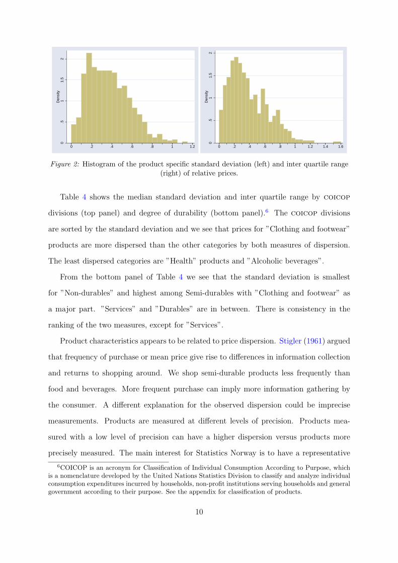
Figure 2 shows the distribution of standard deviations (left panel) and inter quartile

ranges (right) of relative prices (pist) for all 766 products. Both measures of dispersion

varies a lot between products, with the inter quartile range of the standard deviation is

0.303. This means that 50% of the products have a standard deviation between 0.204

and 0.508. For the inter quartile range, 50% of the products have an inter quartile range

between 0.191 and 0.562. The two distributions have a large right tail.

Norway goes from 1,400 per square kilometer in Oslo, the capitol of Norway, to 1.55 per square kilometerin Finmark, the northern mainland of Norway. All numbers are in 2010.

9

0.5

11.

52

Den

sity

0 .2 .4 .6 .8 1 1.2

0.5

11.

52

Den

sity

0 .2 .4 .6 .8 1 1.2 1.4 1.6

Figure 2: Histogram of the product specific standard deviation (left) and inter quartile range(right) of relative prices.

Table 4 shows the median standard deviation and inter quartile range by coicop

divisions (top panel) and degree of durability (bottom panel).6 The coicop divisions

are sorted by the standard deviation and we see that prices for ”Clothing and footwear”

products are more dispersed than the other categories by both measures of dispersion.

The least dispersed categories are ”Health” products and ”Alcoholic beverages”.

From the bottom panel of Table 4 we see that the standard deviation is smallest

for ”Non-durables” and highest among Semi-durables with ”Clothing and footwear” as

a major part. ”Services” and ”Durables” are in between. There is consistency in the

ranking of the two measures, except for ”Services”.

Product characteristics appears to be related to price dispersion. Stigler (1961) argued

that frequency of purchase or mean price give rise to differences in information collection

and returns to shopping around. We shop semi-durable products less frequently than

food and beverages. More frequent purchase can imply more information gathering by

the consumer. A different explanation for the observed dispersion could be imprecise

measurements. Products are measured at different levels of precision. Products mea-

sured with a low level of precision can have a higher dispersion versus products more

precisely measured. The main interest for Statistics Norway is to have a representative

6COICOP is an acronym for Classification of Individual Consumption According to Purpose, whichis a nomenclature developed by the United Nations Statistics Division to classify and analyze individualconsumption expenditures incurred by households, non-profit institutions serving households and generalgovernment according to their purpose. See the appendix for classification of products.

10

Table 4: Median dispersion in relative prices, pist across product categories.

Median

COICOP division N Stdev IQR

Clothing and footwear 102 0.569 0.617Communication 7 0.456 0.588Furnishings, household equip 120 0.425 0.448Restaurants and hotels 38 0.416 0.557Miscellaneous goods, services 60 0.365 0.301Transport 37 0.361 0.305Recreation and culture 81 0.347 0.293Housing, water, electricity, gas and other fuels 15 0.291 0.226Food and non-alcoholic bevs 255 0.272 0.257Alcoholic beverages, tobacco and narcotics 12 0.119 0.112Health 39 0.116 0.063

Semi-durables 184 0.523 0.597Durables 86 0.395 0.384Services 72 0.384 0.447Non-durables 424 0.268 0.243

N is number of products in each category.

consumption basket and track the price development over time. Using the data to to

study price dispersion could therefore suffer from varying precision of the quality and

characteristics of the different products.

Our results of dispersion in prices are in line with other studies. See for example,

Sorensen (2000) for prescription drugs in the US, Lach (2002) for coffee, chicken, flour

and refrigerator in Israel, Hortacsu and Syverson (2004) for mutual funds in the US and

Wildenbeest (2011) for a consumer basket of retail goods in the UK.

3 Method for decomposing the variation in prices

Prices in our data vary considerably across stores and products. We want to use a method

that allows us to decompose the observed variation in prices. Our data contains price

observations on the same good sold in different stores, and the same store selling different

goods. The data structure can be represented by a 2-level cross-classified hierarchy, as

11

Stores

Obs

Products

A B C D

1 2 3

p1Aτ p1Bτ p2Bτ p2Cτ p2Dτ p3Aτ p3Bτ p3Cτ p3Dτ

× × × × × × × × × × × × × × × × × × ×

×××××××××

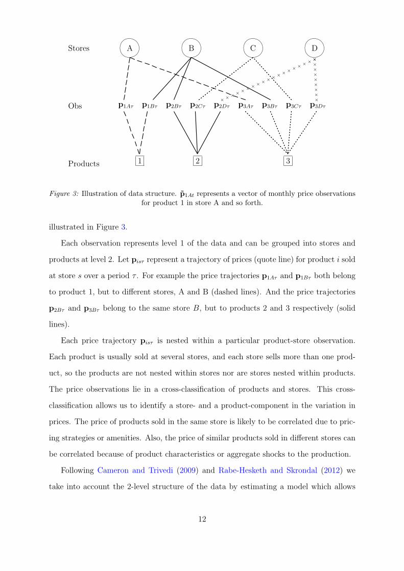
Figure 3: Illustration of data structure. p1At represents a vector of monthly price observationsfor product 1 in store A and so forth.

illustrated in Figure 3.

Each observation represents level 1 of the data and can be grouped into stores and

products at level 2. Let pisτ represent a trajectory of prices (quote line) for product i sold

at store s over a period τ . For example the price trajectories p1Aτ and p1Bτ both belong

to product 1, but to different stores, A and B (dashed lines). And the price trajectories

p2Bτ and p3Bτ belong to the same store B, but to products 2 and 3 respectively (solid

lines).

Each price trajectory pisτ is nested within a particular product-store observation.

Each product is usually sold at several stores, and each store sells more than one prod-

uct, so the products are not nested within stores nor are stores nested within products.

The price observations lie in a cross-classification of products and stores. This cross-

classification allows us to identify a store- and a product-component in the variation in

prices. The price of products sold in the same store is likely to be correlated due to pric-

ing strategies or amenities. Also, the price of similar products sold in different stores can

be correlated because of product characteristics or aggregate shocks to the production.

Following Cameron and Trivedi (2009) and Rabe-Hesketh and Skrondal (2012) we

take into account the 2-level structure of the data by estimating a model which allows

12

for both store- and product-specific random intercepts, taking account of cross effects

between stores and products. The dependent variable is log price, ln pist.

ln pist = βis + eist (2)

where eist ∼ N(0, σ2e) is an error term. The intercept, βis, varies between products and

stores as described by

βis = β0 + ui + vs (3)

where β0 is the fixed global mean of the log prices across products, stores and time,

ui ∼ N(0, σ2u) is a product specific intercept, and vs ∼ N(0, σ2

v) is a store specific intercept.

We interpret ui and vi as random latent factors, assumed to be stochastically independent,

and also independent of the error term eist. The pricing decisions of a store may depend

on idiosyncratic shocks and aggregate shocks at the industry- or country-level (e.g., see

Golosov and Lucas (2007), Mackowiak and Wiederholt (2009) and Taylor (1980)), which

suggest the use of random factors. We want to generalize the decomposed variance of log

prices to other products and stores, not just the once in our sample. Statistics Norway

have randomly selected the stores and products so that they are representative for the

goods and services offered in Norway. Therefore, the products and stores should be

considered random and not fixed factors according to Baltagi (2008) and Rabe-Hesketh

and Skrondal (2012). Combining equations (2) and (3), we get7

pist = β0 + ui + vs + eist (4)

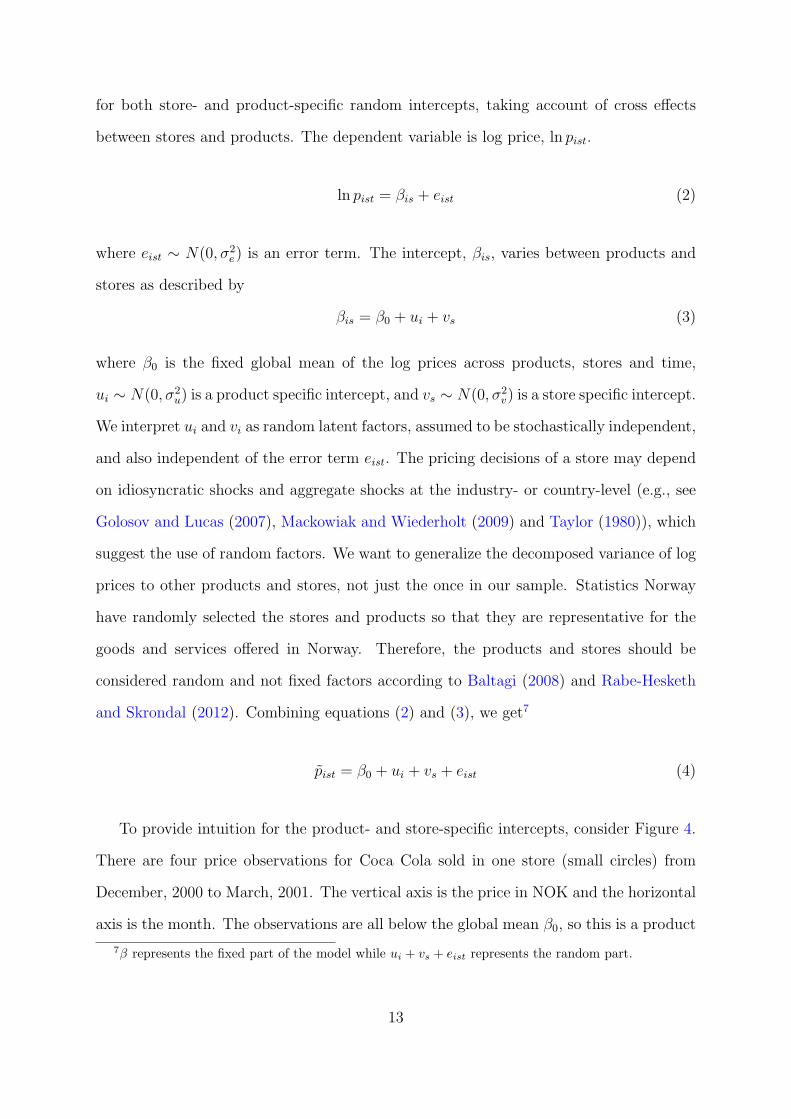
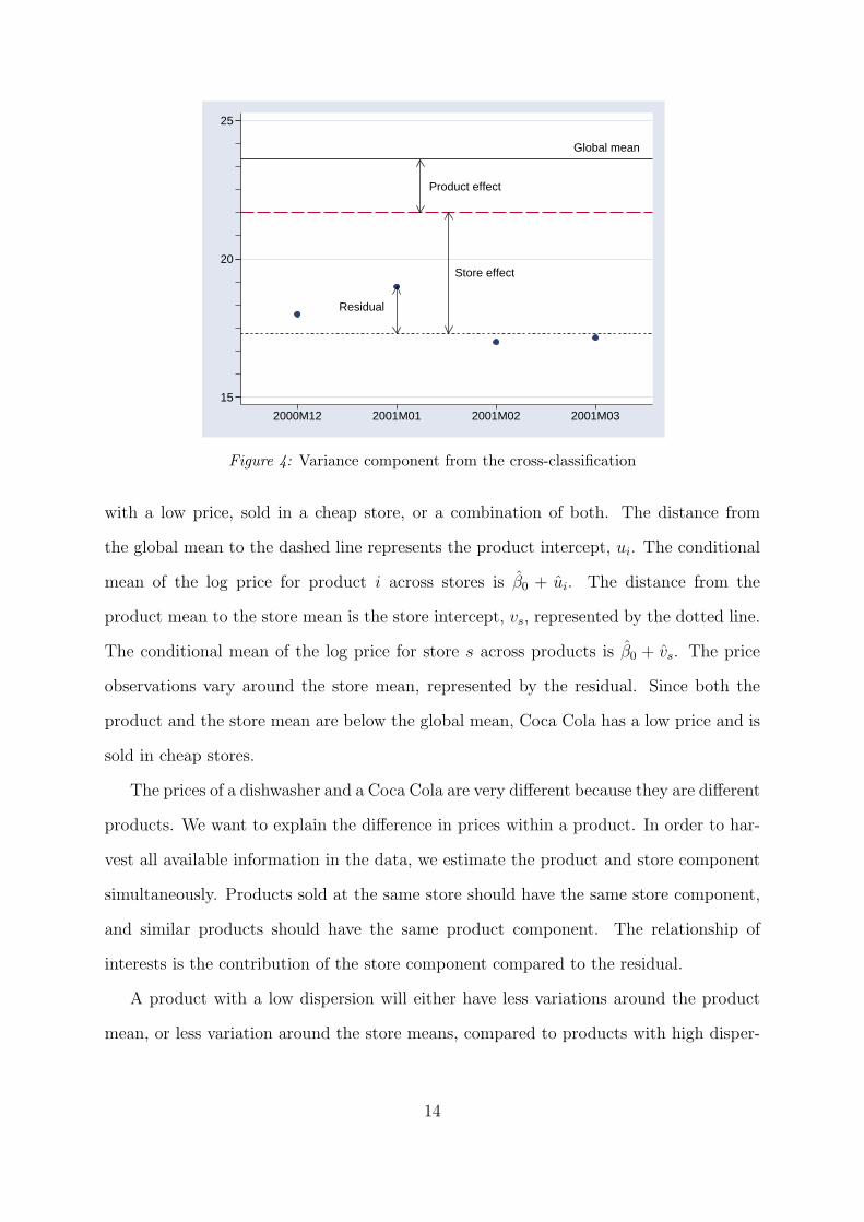
To provide intuition for the product- and store-specific intercepts, consider Figure 4.

There are four price observations for Coca Cola sold in one store (small circles) from

December, 2000 to March, 2001. The vertical axis is the price in NOK and the horizontal

axis is the month. The observations are all below the global mean β0, so this is a product

7β represents the fixed part of the model while ui + vs + eist represents the random part.

13

Global mean

Product effect

Store effect

Residual

15

20

25

2000M12 2001M01 2001M02 2001M03

Figure 4: Variance component from the cross-classification

with a low price, sold in a cheap store, or a combination of both. The distance from

the global mean to the dashed line represents the product intercept, ui. The conditional

mean of the log price for product i across stores is β0 + ui. The distance from the

product mean to the store mean is the store intercept, vs, represented by the dotted line.

The conditional mean of the log price for store s across products is β0 + vs. The price

observations vary around the store mean, represented by the residual. Since both the

product and the store mean are below the global mean, Coca Cola has a low price and is

sold in cheap stores.

The prices of a dishwasher and a Coca Cola are very different because they are different

products. We want to explain the difference in prices within a product. In order to har-

vest all available information in the data, we estimate the product and store component

simultaneously. Products sold at the same store should have the same store component,

and similar products should have the same product component. The relationship of

interests is the contribution of the store component compared to the residual.

A product with a low dispersion will either have less variations around the product

mean, or less variation around the store means, compared to products with high disper-

14

sion. The importance of the two components, store and residual, is determined by their

contributions to dispersion. For example, a store-specific staggered contract (e.g., Taylor

(1980)) would have most of the variability in the distance between the product mean and

the store mean. The variability in the store component would be greater than the vari-

ability in the residual. Industry wide shocks to information structures, for example a ban

on commercials towards children, would have most of the variability between the store

mean and the residual (e.g., Burdett and Judd (1983)). The variability in the residual

component would then be greater than the variability in the store component.

We estimate the parameters β0, σ2u, σ

2v and σ2

e by maximum likelihood. Conditional

on the estimates β0, σ2u, σ

2v and σ2

e we can, according to Rabe-Hesketh and Skrondal

(2012), predict the product and store intercept ui and vs for all products and stores as

the empirical Bayes predictions. Our two prior distributions are normal with mean zero

and estimated variances σ2u and σ2

v . We update our priors with the likelihood of obtaining

the posterior, given the price observations in the data. The empirical Bayes prediction is

the mean of the posterior distribution with parameters β0, σ2u, σ

2v and σ2

e .

The reason we obtain estimates on the random intercepts is because we want to make

inferences on the characteristics of the residuals. We are able to back out the residual

variations after adjusting for product and store factors. The predicator is, according to

Baltagi (2008), the best linear unbiased predicator under the normality assumption of

the residual.

Lach (2002) and Wildenbeest (2011) interpret the residual as the price of a homoge-

neous good adjusted for store and product characteristics. The residuals are normalized

around zero, where below zero is a low price and above zero is a high price. It is the

dispersion in the residual that is of interest, in particular the variance and the properties

of the dispersion.

The assumptions of the stochastic properties of the error terms imply that the variance

of the log price ln pist is

Var(ln pist) = σ2u + σ2

v + σ2e (5)

15

If prices mostly vary between stores, then σ2v will be high relative to the two other

components. If prices vary mostly between products, σ2u will dominate relative to the

other components. Finally, if prices neither vary between stores nor between products,

but due to some other factor, σ2e will be large relative to the two other components.

The relation of interest is the relative importance of the variability between stores for a

product and the residual.

Orange juice can be organic or ordinary. The product component will separate be-

tween coffee and milk, but not within types of orange juice. We expect to capture

persistent quality differences within the product space in our store component. Further-

more, Whole Foods and 7-Eleven both sell orange juice. Store amenities and quality of

service will be captured by the store component. We expect to see much of the variation

captured by the store component if there are for example large differences in the quality

of products or stores in our sample (e.g., Hotelling (1929)).

Price variability between stores can also be consistent with different prices across

regions due to differences in competitive pressure. A stores inability to revise its price can

generates price dispersion if the rigidity is store specific (e.g., Mackowiak and Wiederholt

(2009)). For example, store specific menu costs would be captured in the store component

(e.g., Rotemberg (1982)).

In a model with search frictions (e.g., Burdett and Judd (1983)), the stores are iden-

tical and the dispersion is driven by uncertainty on the consumer side. The dispersion in

prices can then driven by the residual. However, characteristics of the product can drive

the incentives to search, such as the mean price or frequency of purchase as argued by

Stigler (1961). The dispersion in prices can then be driven by the product component.

One alternative estimation procedure would estimate the relationship, per product,

and include a indicator function for each firm. We would not capture the constant

store component across products sold in the same store using this method. The random

intercept model is the parsimonious alternative compared to a fixed-effects model. It

estimates the variance parameters for the product, the store and the residual rather than

16

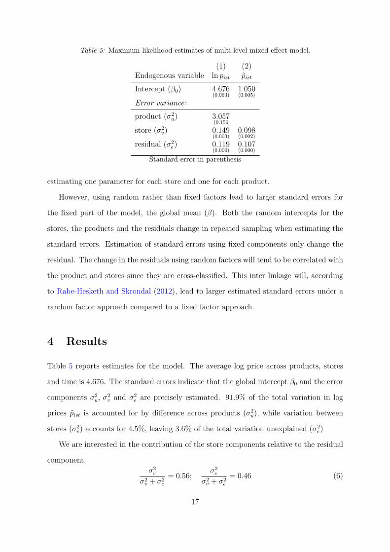
Table 5: Maximum likelihood estimates of multi-level mixed effect model.

(1) (2)Endogenous variable ln pist pist

Intercept (β0) 4.676(0.063)

1.050(0.005)

Error variance:

product (σ2u) 3.057

(0.156

store (σ2v) 0.149

(0.003)0.098(0.002)

residual (σ2e) 0.119

(0.000)0.107(0.000)

Standard error in parenthesis

estimating one parameter for each store and one for each product.

However, using random rather than fixed factors lead to larger standard errors for

the fixed part of the model, the global mean (β). Both the random intercepts for the

stores, the products and the residuals change in repeated sampling when estimating the

standard errors. Estimation of standard errors using fixed components only change the

residual. The change in the residuals using random factors will tend to be correlated with

the product and stores since they are cross-classified. This inter linkage will, according

to Rabe-Hesketh and Skrondal (2012), lead to larger estimated standard errors under a

random factor approach compared to a fixed factor approach.

4 Results

Table 5 reports estimates for the model. The average log price across products, stores

and time is 4.676. The standard errors indicate that the global intercept β0 and the error

components σ2u, σ

2v and σ2

e are precisely estimated. 91.9% of the total variation in log

prices pist is accounted for by difference across products (σ2u), while variation between

stores (σ2v) accounts for 4.5%, leaving 3.6% of the total variation unexplained (σ2

e)

We are interested in the contribution of the store components relative to the residual

component.

σ2v

σ2v + σ2

e

= 0.56;σ2e

σ2v + σ2

e

= 0.46 (6)

17

For the average product, a marginal decomposition the store component account for 56%

of the variability in prices, while the residual account for 46%. The variation between

the residuals is considerable. In column (2), we normalize the prices with the products

monthly mean and inspect the store component relative to the residual. Variation across

stores account for 48% of the variation in relative prices. The residual account for 52%.

The bimodular shape of the relative prices suggest that there are expensive and cheap

stores in our sample. We know differences in quality within a product like cereal or

juice, can be captured as a store component. We therefore caution to attribute the store

component only to store amenities. However, if all the variation in our price were due

to imprecise measurement of the quality of the products, the there should be very little

variation in the residual. Each store reports the price of the same product in every

period. These two results suggest that there is a mix of differences in quality and in

store amenities. Furthermore, the store component can be related to store specific price

rigidities like menu costs (e.g., Rotemberg (1982) or staggered contracts (e.g., Taylor

(1980)). Aggregate shocks at the industry level which are not time-invariant may be

captured in the residual, which is consistent with costless reoptimization but rational

inattention (e.g., Mackowiak and Wiederholt (2009)).

Finally, search models where the dispersion is driven by uncertainty on the consumer

side could have generate some of the variability in the residual since it is not store

specific. However, if two products have different prices, but the same standard deviation,

the monetary returns to finding the lowest price is larger for the product with a higher

price (e.g., Stigler (1961)). This difference in the incentives to shop around making

the equilibrium offered price distribution less dispersed. We could therefore expect to

sell less variability around stores which sells products with a high price. So product

characteristics, like the price, could also explain dispersion due to search frictions.

Wildenbeest (2011) estimates a structural model of product heterogeneity and search

friction. He finds that store heterogeneity explains about 61% of variation in prices, at-

tributing the rest to search frictions. Kaplan and Menzio (2014) find that store amenities

18

and differences in marginal cost only account for 10% of the overall variation in prices.

Lach (2002) finds that store and product characteristics which are time invariant account

for between 47 - 90% of the variation.

Using the estimates from column (1), we predict the posterior product component ui

and store component vs using the empirical Bayesian mean. We predict values for the

product and store intercepts for all products and stores, because we are interested in

characterizing the properties of the distribution of the residual.

eist = ln pist − ui − vs (7)

If all price dispersion is because of product and store time-invariant characteristics, there

should be no dispersion in the residual.

Figure 5 show the distribution of the 766 predicted product effects (left) and the

distribution of the 4297 predicted store effects (right). Product means below (above) zero

have a mean log price below (above) the global mean log price across stores, products

and time. Products in the upper right tail are for example cars. Store means below

(above) zero have a mean log price below (above) the global mean log price across stores,

products and time. A store can sell both expensive products (above zero) and cheap

products (below zero) and still have a store mean below zero. Stores in the left tail are

for example retailing stores, like Target. In the right tail, there are convenience store like

7-Eleven.

The predicted product components are centered around zero with a long right tail.

The predicted store effects are also centered around zero. The interpretation is that the

price of a product is either above or below the global mean across stores, product and

time. The same interpretation goes for a store with a collection of products. The average

price across the stores collection of goods could be cheap or expensive relative to the

average price level across products, stores and time. A product can be cheap relative to

other products, sold in a store cheap store, or a combination of the two. The product

19

0.1

.2.3

Den

sity

−5 0 5 10Estimate

0.5

11.

5D

ensi

ty

−2 −1 0 1 2Estimate

Figure 5: Predicted product effects ui (left) and predicted store effects vs (right) from model(1). Note difference in scale.

Table 6: Descriptive statistics of adjusted prices, εist, across products.

Median Sd Q1 Q3

Sd 0.298 0.202 0.190 0.416Q3–Q1 0.317 0.265 0.201 0.482P95–P5 0.915 0.625 0.578 1.263

could also be cheap relative to other products, but still be sold in an expensive store.

To illustrate the method, Figure 6 shows the store component (vs) in the left panel and

the adjusted log price (i.e. the residuals ε) for Coca Cola. The distribution of the predicted

store component (vs) from the estimated model is bimodal. The store components cannot

account for all of the bimodality in the price distribution (cf. Figure 1) as seen in the

right panel which plots the relative price adjusted for the store and product components.

The modes are smaller and closer than in Figure 1, but still bimodal.

There is still substantial variation in adjusted prices across products even after con-

trolling for product and store components. For the whole sample, the overall standard

deviation in the pooled distribution for all products of adjusted prices (ε) is 0.346, the

IQR is 0.290 and the P95–P5 range is 1.391. Table 6 shows dispersion statistics across

products for the adjusted prices. The median product has a standard deviation of 0.298

and an IQR of 0.317.

20

01

23

Den

sity

−1 −.5 0 .5 1Estimate

01

23

Den

sity

−1 −.5 0 .5 1Resid

Figure 6: Predicted store effects, vs, for stores selling Coca Cola (left) and adjusted relativeprices ϵist (right) from model (2).

5 Conclusion

There is widespread and persistent dispersion in prices for retail goods in Norway from

2000 to 2004. We find that roughly 91.9% of the total variation in price can be attributed

to a product component and 4.5% to a store component. This leaves 3.6% of the total

variation in prices unexplained. We are interested in the decomposition of variability

within each product. We find that 48–56% of the variation is accounted for by a store

component, depending on the regression specification. The residual account for 44–52%.

References

Baltagi, B. (2008). Econometric analysis of panel data. John Wiley & Sons.

Burdett, K. and Judd, K. (1983). Equilibrium price dispersion. Econometrica, 51(4):955–

969.

Calvo, G. (1983). Staggered prices in a utility-maximizing framework. Journal of mone-

tary Economics, 12(3):383–398.

Cameron, A. C. and Trivedi, P. K. (2009). Microeconometrics: Methods and applications.

Cambridge University Press.

21

Diamond, P. (1971). A model of price adjustment. Journal of economic theory, 3(2):156–

168.

Dixit, A. K. and Stiglitz, J. E. (1977). Monopolistic competition and optimum product

diversity. The American Economic Review, pages 297–308.

Golosov, M. and Lucas, R. E. (2007). Menu costs and philips curves. Journal of political

economy, 115:171 – 199.

Hortacsu, A. and Syverson, C. (2004). Product differentiation, search costs, and competi-

tion in the mutual fund industry: A case study of s&p 500 index funds. The Quarterly

Journal of Economics, 119(2):403–456.

Hotelling, H. (1929). Stability in competition. The economic journal, 39(153):41–57.

Kaplan, G. and Menzio, G. (2014). The morphology of price dispersion. NBER Working

Paper 19877.

Lach, S. (2002). Existence and persistence of price dispersion: An empirical analysis.

The Review of Economics and Statistics, 84(3):433–444.

Lancaster, K. (1975). Socially optimal product differentiation. The american economic

review, pages 567–585.

Mackowiak, B. and Wiederholt, M. (2009). Optimal sticky prices under rational inatten-

tion. American Economic Review, 99:769–803.

Mankiw, N. G. and Reis, R. (2002). Sticky information versus sticky prices: a proposal

to replace the new keynesian phillips curve. The Quarterly Journal of Economics,

117(4):1295–1328.

Morgan, P. and Manning, R. (1985). Optimal search. Econometrica: Journal of the

Econometric Society, pages 923–944.

22

Rabe-Hesketh, S. and Skrondal, A. (2012). Multilevel and longitudinal modmodel using

stata. Volume I: Continuous Responses. Stata Press.

Rotemberg, J. (1982). Monopolistic price adjustment and aggregate output. The Review

of Economic Studies, 49(4):517–531.

Sorensen, A. T. (2000). Equilibrium price dispersion in retail markets for prescription

drugs. Journal of Political Economy, 108(4):833–850.

Stigler, G. J. (1961). The economics of information. The journal of political economy,

69(3):213–225.

Taylor, J. B. (1980). Aggregate dynamics and staggered contracts. The Journal of

Political Economy, pages 1–23.

Wildenbeest, M. R. (2011). An empirical model of search with vertically differentiated

products. The RAND Journal of Economics, 42(4):729–757.

A Appendix

A.1 Classification of products according to durability

Non-durable goods

Beer; Bread and cereals; Coffee, tea and cocoa; Electricity; Fish and seafood; Food products

n.e.c.; Fruit; Fuels and lubricants for personal transport equipment; Gardens, plants and flowers;

Heat energy; Liquid fuels; Materials for the maintenance and repair of the dwelling; Meat;

Milk, cheese and eggs; Mineral waters, soft drinks, fruit and vegetable juices; Newspapers

and periodicals; Non-durable household goods; Oils and fats; Other appliances, articles and

products for personal care; Other medical products; Pets and related products; Pharmaceutical

products; Solid fuels; Spirits; Stationery and drawing materials; Sugar, jam, honey, chocolate

and confectionery; Tobacco; Vegetables; Wine.

23

Semi-durable goods

Books; Clothing materials; Electric appliances for personal care; Equipment for sport, camping

and open-air recreation; Games, toys and hobbies; Garments; Glassware, tableware and house-

hold utensils; Household textiles; Other articles of clothing and clothing accessories; Other per-

sonal effects; Recording media; Shoes and other footwear; Small electric household appliances;

Small tools and miscellaneous accessories; Spare parts and accessories for personal transport

equipment

Durable goods

Bicycles; Carpets and other floor coverings; Equipment for the reception, recording and repro-

duction of sound and pictures; Furniture and furnishings; Information processing equipment;

Jewellery, clocks and watches; Major durables for outdoor recreation; Major household appli-

ances whether electric or not; Major tools and equipment; Motor cars; Motor cycles; Musical

instruments and major durables for indoor recreation; Photographic and cinematographic equip-

ment and optical instruments; Telephone and telefax equipment; Therapeutic appliances and

equipment.

Services

Accommodation services; Actual rentals paid by tenants; Canteens; Cleaning, repair and hire of

clothing; Cultural services; Dental services; Domestic services and household services; Hairdress-

ing salons and personal grooming establishments; Imputed rentals of owner-occupiers; Insurance

connected with the dwelling; Insurance connected with transport; Maintenance and repair of

personal transport equipment; Medical services; Other actual rentals; Other financial services

n.e.c.; Other imputed rentals; Other services in respect of personal transport equipment; Other

services n.e.c.; Package holidays; Paramedical services; Passenger transport by air; Passenger

transport by railway; Passenger transport by road; Passenger transport by sea and inland wa-

terway; Postal services; Pre-primary and primary education; Recreational and sporting services;

Repair and hire of footwear; Repair of audio-visual, photographic and information processing

equipment; Repair of household appliances; Restaurants, cafnd the like; Secondary education;

24

Services for the maintenance and repair of the dwelling; Social protection; Telephone and telefax

services; Tertiary education.

25