Embed Size (px)
Citation preview
DISSERTATION
TURBULENT VELOCITY PROFILES IN CLEAR WATER AND
SEDIMENT-LADEN FLOWS
Submitted by
Junke Guo
Department of Civil Engineering
In partial fulÞllment of the requirements
for the Degree of Doctor of Philosophy
Colorado State University
Fort Collins, Colorado
Spring 1998
COLORADO STATE UNIVERSITY
December 18, 1997
WE HEREBY RECOMMEND THAT THE DISSERTATION PREPARED
UNDER OUR SUPERVISION BY JUNKE GUO ENTITLED TURBULENT
VELOCITY PROFILES IN CLEAR WATER AND SEDIMENT-LADEN
FLOWS BE ACCEPTED AS FULFILLING IN PART REQUIREMENTS FOR
THE DEGREE OF DOCTOR OF PHILOSOPHY.
Committee on Graduate Work
Adviser
Department Head/Director

To my parents
my brothers and sisters
my wife Jun An and my son Hao
Everything should be made as simple as possible,
but not simpler.
Albert Einstein
ABSTRACT OF DISSERTATION
TURBULENT VELOCITY PROFILES IN CLEAR WATER AND
SEDIMENT-LADEN FLOWS
This dissertation studies turbulent velocity proÞles in pipes with clear water, and
centerline velocity proÞles in open-channels with clear water and sediment-laden ßows.
The main purpose is to Þnd a suitable velocity proÞle law for the entire boundary
layer, particularly near the water surface, and to study the effects of sediment suspen-
sion on the model parameters. As a prerequisite for the study of velocity proÞles in
open-channels, a theoretical method for determining the bed shear stress in smooth
rectangular channels is presented.
The major Þndings are:
(1) A wall shear turbulent velocity proÞle, in a velocity defect form, consists of
three parts: a log term, a wake correction term, and a boundary correction term which
is a linear function. The Þrst two terms are the same as those in the classical log-wake
law. The third term is a major contribution of this study. This new velocity proÞle
law is referred to as the modiÞed log-wake law. The new law considers the upper
derivative boundary condition, which is not satisÞed in previous studies. Physically,
the log term reßects the inertia effect, the wake term reßects the large scale turbulent
mixing, and the linear term reßects the effect of the upper boundary condition. In
open-channels, the log term reßects the effect of the channel bed; the wake term
reßects the effect of the side-walls, which induce secondary ßows in the corners and
then produce large scale turbulent mixing.
(2) For clear water ßows in pipes, the new law contains two universal constants:
the von Karman constant κ0 = 0.406 and the wake strength coefficient Ω0 = 3.2.
(3) For clear water ßows in narrow channels, the boundary layer thickness δ is
vii
deÞned as the distance from the bed to the maximum velocity. The velocity proÞle
equation is similar to that in pipes except that the wake strength coefficient Ω0
decreases with the aspect ratios. In particular, the new law can even reproduce the
velocity proÞle measurements beyond the boundary layer thickness.
(4) For clear water ßows in wide channels, the effect of the side-walls is weakened,
also, the water surface limits large scale turbulent mixing, so the wake component
may be neglected. The modiÞed log-wake law reduces to a log-linear law. The von
Karman constant κ0 is still 0.406. The water surface shear stress is considered through
the parameter λ0 which is about a constant 0.065 for a smooth bed and small relative
roughness, but increases with the relative roughness in very rough beds.
(5) The modiÞed log-wake law is also valid in sediment-laden ßows. Sediment
suspension affects the velocity proÞle in two factors: concentration and density gra-
dient (the Richardson number Ri). Both factors reduce the von Karman constant κ.
However, if both concentration and density gradient near the water surface are very
small, they have little effect on the wake strength coefficient Ω in narrow channels
and the water surface shear effect factor λ in wide channels.
(6) The modiÞed log-wake law, including its reduction in wide channels, compares
quite well with over 100 experimental velocity proÞles in pipes, narrow open-channels
and wide open-channels. The correlation coefficients r are always over 0.99.
Junke GuoDepartment of Civil EngineeringColorado State UniversityFort Collins, CO 80523Spring 1998
viii
ACKNOWLEDGMENTS
I would like to thank a number of people who contributed, directly or indirectly,
to this dissertation. First, I would like to express gratitude to Prof. Pierre Y. Julien,
my advisor, for his guidance, encouragement, friendship and Þnancial support during
this study. Working with him has been a rewarding and enjoyable experience.
Prof. Carl F. Nordin and Prof. Robert N. Meroney expressed much interest in
this study. Their service in my graduate study committee and academic supports are
greatly appreciated. Thanks do also go to Prof. Deborah J. Anthony at Department
of Earth Resources for her service as the outside member in the committee.
The experimental data used in this dissertation were provided by Dr. Lex Smits
and Dr. Mark V. Zagarola at Princeton University, Dr. Walter H. Graf at Swiss
Federal Institute of Technology at Lausanne, Dr. Marian V. I. Muste at the University
of Iowa, and Dr. Xang-Kui Wang and Prof. Yu-Jia Hui at Tsinghua University,
China. These people are greatly acknowledged. Their valuable data sets are certainly
important for this study.
I am also grateful to Dr. Virenda C. Patel, Distinguished Professor and Director
of Iowa Institute of Hydraulic Research, the University of Iowa, and Prof. Yu-Jia Hui
at the Sedimentation Lab, Tsinghua University, China, for their constant encourage-
ment. Mr. Baosheng Wu, my classmate in both China and CSU, is also appreciated
for his discussion, encouragement and friendship.
In addition, I particularly thank Dr. Hsieh Wen Shen, Professor of Civil and Envi-
ronmental Engineering at the University of California, Berkeley, Member of National
Academy of Engineering, for his support through the 1997-1998 H. W. Shen Water
Resources Graduate Award.
Lastly, I would like to dedicate this work to my parents, brothers and sisters. Their
twenty year supports make this dissertation possible. I would also like to dedicate
ix
this work to my wife Jun An and my son Hao Guo for their patience, understanding,
and love through the two years required for this effort.
Junke GuoDivision of Hydraulics and Fluid MechanicsDepartment of Civil EngineeringColorado State UniversityFort Collins, CO [email protected]
x
Contents
1 INTRODUCTION 1
1.1 Statement and signiÞcance of the problem . . . . . . . . . . . . . . . 1
1.2 Background . . . . . . . . . . . . . . . . . . . . . . . . . . . . . . . . 1
1.3 Objectives . . . . . . . . . . . . . . . . . . . . . . . . . . . . . . . . . 2
1.4 Limitations and assumptions . . . . . . . . . . . . . . . . . . . . . . . 2
1.5 Outline . . . . . . . . . . . . . . . . . . . . . . . . . . . . . . . . . . . 3
2 LITERATURE REVIEW 4
2.1 Introduction . . . . . . . . . . . . . . . . . . . . . . . . . . . . . . . . 4
2.2 Velocity ProÞle in Clear Water . . . . . . . . . . . . . . . . . . . . . . 4
2.2.1 Linear law in the viscous sublayer . . . . . . . . . . . . . . . . 5
2.2.2 Log law in the overlap . . . . . . . . . . . . . . . . . . . . . . 6
2.2.3 Parabolic law in the wake layer and upper boundary conditions 7
2.2.4 The law of the wall (general inner region law) . . . . . . . . . 10
2.2.5 The law of the wake (general outer region law) . . . . . . . . . 11
2.3 Velocity ProÞles in Sediment-Laden Flows . . . . . . . . . . . . . . . 12
2.3.1 Extension of the log law to sediment-laden ßows . . . . . . . . 12
2.3.2 Extension of the log-wake law to sediment-laden ßows . . . . . 14
2.3.3 Log-linear law and others . . . . . . . . . . . . . . . . . . . . 16
2.4 Summary . . . . . . . . . . . . . . . . . . . . . . . . . . . . . . . . . 17
3 SIMILARITY ANALYSIS OF CLEAR WATER VELOCITY PRO-
FILES 18
xi
3.1 Introduction . . . . . . . . . . . . . . . . . . . . . . . . . . . . . . . . 18
3.2 Four-step similarity analysis method . . . . . . . . . . . . . . . . . . 19
3.2.1 Dimensional analysis . . . . . . . . . . . . . . . . . . . . . . . 19
3.2.2 Intermediate asymptotics . . . . . . . . . . . . . . . . . . . . . 20
3.2.3 Wake correction (or wake function) . . . . . . . . . . . . . . . 20
3.2.4 Boundary correction . . . . . . . . . . . . . . . . . . . . . . . 21
3.3 Velocity proÞle analysis . . . . . . . . . . . . . . . . . . . . . . . . . . 23
3.3.1 Dimensional analysis . . . . . . . . . . . . . . . . . . . . . . . 23
3.3.2 Intermediate asymptotics . . . . . . . . . . . . . . . . . . . . . 24
3.3.3 Wake correction to the log law . . . . . . . . . . . . . . . . . . 25
3.3.4 Boundary correction to the log-wake law . . . . . . . . . . . . 26
3.4 Implication to turbulent eddy viscosity . . . . . . . . . . . . . . . . . 27
3.5 Summary . . . . . . . . . . . . . . . . . . . . . . . . . . . . . . . . . 28
4 SHEAR VELOCITY IN SMOOTH OPEN-CHANNELS 29
4.1 Introduction . . . . . . . . . . . . . . . . . . . . . . . . . . . . . . . . 29
4.2 Conformal mapping from a rectangular cross-section (z-plane) into a
half upper plane (w-plane) . . . . . . . . . . . . . . . . . . . . . . . . 30
4.3 Bed shear stress distribution and centerline shear velocity . . . . . . . 32
4.4 Average bed shear stress and average bed shear velocity . . . . . . . . 36
4.5 Summary . . . . . . . . . . . . . . . . . . . . . . . . . . . . . . . . . 41
5 TEST OF THE MODIFIED LOG-WAKE LAW IN CLEAR WA-
TER 42
5.1 Introduction . . . . . . . . . . . . . . . . . . . . . . . . . . . . . . . . 42
5.2 Test of the modiÞed log-wake law in pipes . . . . . . . . . . . . . . . 43
5.2.1 ModiÞed log-wake law in pipes . . . . . . . . . . . . . . . . . . 43
5.2.2 Data selection . . . . . . . . . . . . . . . . . . . . . . . . . . . 43
5.2.3 Methods for determining κ0 and Ω0 . . . . . . . . . . . . . . . 43
5.2.4 Test of the structure of the modiÞed log-wake law . . . . . . . 45
5.2.5 Test of κ0 and Ω0 with Reynolds number . . . . . . . . . . . . 45
xii
5.2.6 Test of the eddy viscosity model . . . . . . . . . . . . . . . . . 49
5.3 Test of the modiÞed log-wake law in narrow open-channels . . . . . . 53
5.3.1 Data selection . . . . . . . . . . . . . . . . . . . . . . . . . . . 53
5.3.2 Method for determining δ and u1max . . . . . . . . . . . . . . 54
5.3.3 Test of the modiÞed log-wake law . . . . . . . . . . . . . . . . 54
5.3.4 Test of the eddy viscosity model . . . . . . . . . . . . . . . . . 60
5.4 Test of the modiÞed log-wake law in wide open-channels . . . . . . . 61
5.4.1 Data selection . . . . . . . . . . . . . . . . . . . . . . . . . . . 61
5.4.2 Method for determining u∗, Ω0, and λ0 . . . . . . . . . . . . . 61
5.4.3 Test of the modiÞed log-wake law . . . . . . . . . . . . . . . . 61
5.4.4 Wake strength coefficient Ω0 in open-channels . . . . . . . . . 62
5.5 SimpliÞcation of the modiÞed log-wake law and its test in wide open-
channels . . . . . . . . . . . . . . . . . . . . . . . . . . . . . . . . . . 64
5.5.1 SimpliÞcation of the modiÞed log-wake law (the log-linear law)
in wide open-channels . . . . . . . . . . . . . . . . . . . . . . 64
5.5.2 Data selection . . . . . . . . . . . . . . . . . . . . . . . . . . . 65
5.5.3 Method for determining u∗, λ0 and u1max . . . . . . . . . . . . 66
5.5.4 Test of the log-linear law . . . . . . . . . . . . . . . . . . . . . 66
5.5.5 The water surface shear effect factor λ0 . . . . . . . . . . . . . 67
5.5.6 Test of the eddy viscosity model . . . . . . . . . . . . . . . . . 73
5.6 Summary . . . . . . . . . . . . . . . . . . . . . . . . . . . . . . . . . 75
6 THEORETICAL ANALYSIS OF SEDIMENT-LADEN FLOWS 77
6.1 Introduction . . . . . . . . . . . . . . . . . . . . . . . . . . . . . . . . 77
6.2 Governing equations . . . . . . . . . . . . . . . . . . . . . . . . . . . 77
6.2.1 Navier-Stokes equations in sediment-laden ßows . . . . . . . . 77
6.2.2 Reynolds mean equations and turbulent equations in sediment-
laden ßows . . . . . . . . . . . . . . . . . . . . . . . . . . . . . 79
6.3 SimpliÞcations of governing equations in steady uniform 2D ßows . . 82
6.4 Effects of sediment suspension on turbulence intensities . . . . . . . . 86
xiii
6.4.1 Turbulence intensity u0iu0j in sediment-laden ßows . . . . . . . 87
6.4.2 Turbulent kinetic energy budget and Richardson number in
sediment-laden ßows . . . . . . . . . . . . . . . . . . . . . . . 89
6.4.3 Effects of sediment suspension on the vertical eddy viscosity . 91
6.5 ModiÞcation of the eddy viscosity model in sediment-laden ßows . . . 93
6.6 Velocity proÞles in sediment-laden ßows . . . . . . . . . . . . . . . . 94
6.7 Summary . . . . . . . . . . . . . . . . . . . . . . . . . . . . . . . . . 94
7 TEST OF THE MODIFIED LOG-WAKE LAW IN SEDIMENT-
LADEN FLOWS 96
7.1 Introduction . . . . . . . . . . . . . . . . . . . . . . . . . . . . . . . . 96
7.2 Preliminary analysis of the model parameters . . . . . . . . . . . . . 96
7.3 Test of the modiÞed log-wake law in narrow open-channels . . . . . . 97
7.3.1 Effect of molecular viscosity . . . . . . . . . . . . . . . . . . . 98
7.3.2 Effect of density gradient . . . . . . . . . . . . . . . . . . . . . 104
7.3.3 Combination of the effects of molecular viscosity and density
gradient . . . . . . . . . . . . . . . . . . . . . . . . . . . . . . 109
7.4 Test of the log-linear law in natural rivers . . . . . . . . . . . . . . . 110
7.4.1 Test of the log-linear law in natural rivers . . . . . . . . . . . 110
7.4.2 Conjecture of the effects of sediment suspension in wide open-
channels . . . . . . . . . . . . . . . . . . . . . . . . . . . . . . 111
7.5 Summary . . . . . . . . . . . . . . . . . . . . . . . . . . . . . . . . . 114
8 APPLICATIONS OF THE MODIFIED LOG-WAKE LAW 115
8.1 Applications of the modiÞed log-wake law in pipes . . . . . . . . . . . 115
8.1.1 Relation between the maximum velocity u1max and the average
velocity U . . . . . . . . . . . . . . . . . . . . . . . . . . . . . 115
8.1.2 Position of the average velocity U . . . . . . . . . . . . . . . . 116
8.1.3 Procedures for applying the modiÞed log-wake law . . . . . . . 116
8.2 Applications of the modiÞed log-wake law in open-channels . . . . . . 117
8.2.1 Magnitude of the linear term in the log-linear law . . . . . . . 118
xiv
8.2.2 Relation between the maximum velocity u1max and the average
velocity U . . . . . . . . . . . . . . . . . . . . . . . . . . . . . 118
8.2.3 Position of the average velocity U . . . . . . . . . . . . . . . . 119
8.2.4 Procedures for applying the log-linear law . . . . . . . . . . . 120
9 SUMMARY AND CONCLUSIONS 122
9.1 Summary . . . . . . . . . . . . . . . . . . . . . . . . . . . . . . . . . 122
9.2 Conclusions . . . . . . . . . . . . . . . . . . . . . . . . . . . . . . . . 123
9.2.1 Clear water ßows . . . . . . . . . . . . . . . . . . . . . . . . . 123
9.2.2 Sediment-laden ßows . . . . . . . . . . . . . . . . . . . . . . . 125
9.3 Recommendations . . . . . . . . . . . . . . . . . . . . . . . . . . . . . 126
REFERENCES 127
APPENDICES 133
A POWER-WAKE LAW IN TURBULENT PIPE FLOWS 133
Development of the power-wake law . . . . . . . . . . . . . . . . . . . . . . 133
Dimensional analysis . . . . . . . . . . . . . . . . . . . . . . . . . . . 133
Intermediate asymptotics . . . . . . . . . . . . . . . . . . . . . . . . . 134
Wake correction . . . . . . . . . . . . . . . . . . . . . . . . . . . . . . 134
Boundary correction . . . . . . . . . . . . . . . . . . . . . . . . . . . 134
Determinations of α and Co in the power-wake law . . . . . . . . . . . . . 135
Test of the power-wake law . . . . . . . . . . . . . . . . . . . . . . . . . . 136
B MATLAB PROGRAMS 140
Program for solving κ and Ω in the modiÞed log-wake law . . . . . . . . . 140
Program for solving κ, u1max and λ in the log-linear law . . . . . . . . . . . 143
C ANALYSIS OF WANG-QIANS EXPERIMENTAL DATA 145
Introduction of the experiments . . . . . . . . . . . . . . . . . . . . . . . . 145
Measurements of velocity proÞle and concentration proÞle data (Wang and
Qian, 1989) . . . . . . . . . . . . . . . . . . . . . . . . . . . . . . . . 146
xv
Velocity proÞle analysis . . . . . . . . . . . . . . . . . . . . . . . . . . . . 146
D ANALYSIS OF COLEMANS EXPERIMENTAL DATA 173
E ANALYSIS OF KIRONOTOS EXPERIMENTAL DATA 197
F ANALYSIS OF MUSTES EXPERIMENTAL DATA 216
G ANALYSIS OF McQUIVEYS EXPERIMENTAL DATA 220
H ANALYSIS OF GUY, SIMONS AND RICHARDSONS EXPERI-
MENTAL DATA 228
I MEASUREMENT DATA IN THE YELLOW RIVER AND THE
YANGTZE RIVER 234
Measurements of velocity and concentration proÞles at Hua-Yuan-Kou Hy-
drologic Station, the Yellow River, China . . . . . . . . . . . . . . . . 234
Measurements of velocity and concentration proÞles at Feng-Jie Hydrologic
Station, the Yangtze River, China . . . . . . . . . . . . . . . . . . . . 236
xvi
List of Tables
4.1 Comparison of side-wall correction factor with experiments . . . . . 40
5.1 The model parameters in the modiÞed log-wake law for individual ve-
locity proÞles (Velocity proÞle data source: Zagarola, 1996) . . . . . 48
5.2 Calculated results of Wang-Qians clear and salt water experiments . 55
5.3 Calculated results of Colemans clear water experiments . . . . . . . 55
5.4 Calculated results of Kironotos clear water experiments . . . . . . . 59
5.5 Results of Kironotos wide channel experiments from the modiÞed log-
wake law . . . . . . . . . . . . . . . . . . . . . . . . . . . . . . . . . 62
5.6 Results of Kironotos wide channel experiments . . . . . . . . . . . . 67
5.7 Results of Mustes wide channel experiments . . . . . . . . . . . . . 67
5.8 Results of McQuiveys wide channel experiments . . . . . . . . . . . 68
5.9 Results of Guy et al.s wide channel experiments . . . . . . . . . . . 68
7.1 Calculated results of Wang-Qians neutral particle experiments . . . 101
7.2 Calculated results of Wang-Qians quasi-neutral particle experiments 102
A.1 The model parameters in the power-wake law for individual velocity
proÞles (Velocity proÞle data source: Zagarola, 1996) . . . . . . . . . 137
C.1 Wang-Qians (1989) measurements of velocity proÞles in clear water
and salt water . . . . . . . . . . . . . . . . . . . . . . . . . . . . . . . 147
C.2 Wang-Qians (1989) measurements of velocity proÞles in neutral particle-
laden ßows . . . . . . . . . . . . . . . . . . . . . . . . . . . . . . . . . 148
xvii
C.3 Wang-Qians (1989) measurements of velocity proÞles in density sediment-
laden ßows . . . . . . . . . . . . . . . . . . . . . . . . . . . . . . . . . 149
C.4 Wang-Qians (1989) measurements of concentration proÞles . . . . . . 151
D.1 Colemans (1986) measurement data of velocity and concentration pro-
Þles . . . . . . . . . . . . . . . . . . . . . . . . . . . . . . . . . . . . . 174
E.1 Kironotos (1993) measurement data . . . . . . . . . . . . . . . . . . 198
F.1 Mustes (1995)a measurements of velocity proÞles . . . . . . . . . . . 217
G.1 McQuiveys (1971) measurements of velocity proÞles . . . . . . . . . . 221
H.1 Selected experimental data of Guy, Simons and Richardson (1966) . . 229
xviii
List of Figures
2.1 Sketch of a representative velocity proÞle in open-channels . . . . . . 5
2.2 Upper derivative boundary conditions in pipes, narrow channels (a/h <
5), and wide channels (a/h ≥ 5) . . . . . . . . . . . . . . . . . . . . . 9
2.3 The velocity defect law in the outer region (After Hinze, 1975, p.631) 10
2.4 The law of the wall in the inner region (After White, 1991, p.416) . . 11
2.5 Effect of suspended sediment on the von Karman constant (After Ein-
stein and Chien, 1955) . . . . . . . . . . . . . . . . . . . . . . . . . . 13
2.6 Effect of suspended sediment on the wake strength coefficient . . . . . 15
4.1 Scheme of ßow domain from a rectangular cross-section to a half upper
plane . . . . . . . . . . . . . . . . . . . . . . . . . . . . . . . . . . . . 31
4.2 Scheme for computing bed shear stress distribution . . . . . . . . . . 33
4.3 Bed shear stress distribution versus aspect ratio . . . . . . . . . . . . 35
4.4 Scheme for computing average bed shear stress . . . . . . . . . . . . . 37
4.5 Comparison of the theoretical side-wall correction factor with experi-
mental data . . . . . . . . . . . . . . . . . . . . . . . . . . . . . . . . 39
5.1 Test of the structure of the modiÞed log-wake law [(a) in a semilog
coordinate system; (b) in a rectangular coordinate system.] . . . . . 46
5.2 Comparison of the modiÞed log-wake law and Zagarolas superpipe
experimental proÞles with y+ ≥ 70 . . . . . . . . . . . . . . . . . . . 47
5.3 (a) Variation of κ0 versus Re∗; (b) Variation of Ω0 versus Re∗ . . . . 50
5.4 Complete similarity: Comparison of the modiÞed log-wake law with
Zagarolas (1996) superpipe experimental data with y+ ≥ 500 . . . . 51
xix
5.5 Test of the eddy viscosity model from the modiÞed log-wake law . . . 52
5.6 Comparison of the modifed log-lake law with Wang-Qians experiments
[(a) in a semilog coordinate system, (b) in a rectangular coordinate
system] . . . . . . . . . . . . . . . . . . . . . . . . . . . . . . . . . . 56
5.7 Comparison between the modifed log-lake law and Colemans experi-
mental data [(a) in a semilog coordinate system , (b) in a rectangular
coordinate system] . . . . . . . . . . . . . . . . . . . . . . . . . . . . 57
5.8 Comparison between the modifed log-lake law and Kironotos narrow
ßume data [(a) in a semilog coordinate system, (b) in a rectangular
coordinate system] . . . . . . . . . . . . . . . . . . . . . . . . . . . . 58
5.9 Test of the eddy viscosity model from the modiÞed log-wake law . . . 60
5.10 Comparison of the modiÞed log-wake law with Kironotos wide channel
data [(a) in a rectangular coordinate, (b) in a semilog coordinate] . . 63
5.11 The wake strength coefficient Ω0 versus the aspect ratio a/h . . . . . 64
5.12 Comparison of the log-linear law with Kironotos experimental data
[(a) in a rectangular coordinate, (b) in a semilog coordinate] . . . . . 69
5.13 Comparison between the log-linear law and Mustes experimental data
[(a) in a rectangular coordinate, (b) in a semilog coordinate] . . . . . 70
5.14 Comparison between the log-linear law and McQuiveys experimental
data [(a) in a rectangular coordinate, (b) in a semilog coordinate] . . 71
5.15 Comparison between the log-linear law and Guy et al.s experimental
data [(a) in a rectangular coordinate system, (b) in a semilog coordi-
nate system] . . . . . . . . . . . . . . . . . . . . . . . . . . . . . . . 72
5.16 The water surface effect factor λ0 . . . . . . . . . . . . . . . . . . . . 74
5.17 Test of the eddy viscosity model from the log-linear law . . . . . . . . 75
6.1 Scheme of steady uniform 2D sediment-laden ßows . . . . . . . . . . 83
7.1 A representative velocity proÞle of neutral sediment-laden ßows in nar-
row channels [(a) in a semilog coordinate; (b) in a rectangular coordi-
nate] . . . . . . . . . . . . . . . . . . . . . . . . . . . . . . . . . . . . 99
xx
7.2 The effect of molecular viscosity on the velocity proÞles [o: Wang and
Qians data (1989); : The modiÞed log-wake law] . . . . . . . . . . 100
7.3 The effect of molecular viscosity on the von Karman constant . . . . 103
7.4 The effect of molecular viscosity on the wake strength coefficient . . . 103
7.5 A representative velocity proÞle of sediment-laden ßows in narrow
channels [(a) in a semilog coordinate; (b) in a rectangular coordinate] 105
7.6 The effect of density gradient on velocity proÞles [o: Colemans data
(1986); : The modiÞed log-wake law] . . . . . . . . . . . . . . . . . 106
7.7 The effect of density gradient on the von Karman constant . . . . . . 109
7.8 The effect of density gradient on the wake strength coefficient . . . . 110
8.1 Position of the average velocity versus the water surface shear correction119
A.1 Comparison among the power-wake law, the modiÞed log-wake law and
Zagarolas superpipe experimental data (y+ ≥ 50) . . . . . . . . . . . 138
A.2 The variations of the model parameters with Reynolds number: (a) α
versus Re∗, (b) Co versus Re∗ . . . . . . . . . . . . . . . . . . . . . . 139
xxi
List of Symbols
A Constant in parabolic law (2.17)
Ab, Aw Cross-section areas corresponding to the bed and the side-walls,
respectively, see FIG. 4.2
a Channel width
a1, a2, a3 Curve-Þtting constant in the parabolic law (5.14)
B (= 5.5) constant in Spaldings law (2.18); or boundary correction
function in (3.6), (3.7) and (3.22)
C Instantaneous volumetric sediment concentration
C Local time-mean volumetric sediment concentration
Ca Reference volumetric sediment concentration
Cd Water surface drag coefficient in (2.10)
Ci Parameter in the power law (A.4)
Co Parameter in the power law (A.5)
C1, C2 Addictive constants in the log law (2.6) and (2.21)
C3 Constant in the log-wake law (3.21)
C4 Addictive constant in the power law (A.4)
D Molecular sediment diffusion coefficient in (6.3)
d Pipe diameter
ds Sediment diameter
d50 Sediment medium diameter
F Functional symbols in (3.9), (3.10) and (6.55)
F1, F2 Functional symbols in (7.1), and (7.2)
f Functional symbols in (3.8), (6.8) and FIG. (4.2)
xxii
G (= ρs/ρ0) speciÞc gravity; or functional symbols in (3.12) and (3.13)
g The gravitational acceleration; or functional symbol in (3.11)
gi Component of the gravitational acceleration in the xi−directionh Flow depth
i, j, k Subscripts in tensor variables
ks Bed roughness
Lm Monin-Obukhov length scale in (2.21)
m Subscript for mixture water; or exponent in (7.9)
n Sample number of a velocity proÞle measurements
p Pressure
p1, p2, p3 Curve-Þtting constants in (5.20) and (5.25)
R Pipe radius or hydraulic radius
Ri Global Richardson number in (6.45)
r Correlation coefficient of the modiÞed log-wake law with measurement
velocity proÞle data
Re (= V R/ν) Reynolds number
Re∗ (= u∗δ/ν) Reynolds number
S Energy or bed slope; or the sum of the squares of residuals in the
least-squares method (5.3)
t Time
U Pipe average velocity, or vertical average velocity in an open-channel
ui Instantaneous velocity in direction−i, and i = 1, 2, 3. 1 denotes theßow direction; 2 denotes the lateral direction; and 3 denotes the
vertical direction
ui Local time-mean; or sample data in a curve-Þtting
u0i Turbulent velocity
u∗ Shear velocity
u1max The maximum velocity at the boundary layer margin ξ = 1
u+ (= u1/u∗) normalized velocity by the shear velocity
u0iu0j Turbulence intensity
xxiii
Vwind Wind velocity over the water surface
W Wake function
w A half-upper plane, complex variable w = ξ + iη
xi Coordinates
x1 Flow direction coordinate; or a point in the bed of FIG. 4.2
x30 Reference position in the Monin-Obukhov log-linear law in (2.21)
y+ (= u∗x3/ν) normalized distance by the viscous length scale
z Physical ßow domain, complex varible z = x+ iy
Greek Symbols
α Coefficient in (7.5); or exponent in the power law (A.3)
αi Experimental exponents in a complete similarity (3.3)
β Coefficient in (7.8)
Γ Symbol of a boundary
δ Boundary layer thickness, which is deÞned as the distnace from the bed
to the maximum velocity position
ε Turbulent eddy viscosity
εm Eddy viscosity in sediment-laden ßows
ε+ Dimensionless turbulent eddy viscosity
ε+m Dimensionless eddy viscosity in sediment-laden ßows
εs Dimensionless turbulent sediment diffusion coefficient
ε+1 Dimensionless eddy viscosity at the water surface ξ = 1 for wide open-
channels in (2.11)
κ The von Karman constant in sediment-laden ßows
κ0 The von Karman constant in clear water (κ0 = 0.406)
λ Secondary ßow correction for an average bed shear stress in (4.21) and
(4.22); or water surface shear effect factor in the log-linear law in
wide open-channels
xxiv
λ0 Water surface shear effect factor in the log-linear law in clear water ßows
µ The kinetic viscosity of clear water
µm The kinetic viscosity of mixture water
ν The kinematic viscosity of clear water
νm The kinematic viscosity of mixture water
Π The Coles wake strength coefficient in (2.19) or a dependable similarity
parameter
Πi Independent similarity variables, and i = 1, 2, 3, · · · ,mρ Local sediment-water mixture density
ρ0 The water density
ρair Air density over a water surface, ρair = 1.21 kg/m3 is taken in this study
τb Local bed shear stress
τ b Average bed shear stress
τbc Channel centerline bed shear stress
τ0 Bed shear stress in a 2D open-channel
ξ (= x3/δ) Sample data in a curve-Þtting
ξ Position of the average velocity in a pipe or an open-channel ßow
Ω Wake strength coefficient
Ω0 Wake strength coefficient in clear water ßows
ω Sediment settling velocity
Φ Functional symbol of a similarity analysis in (3.1)
Φs A concentration correction factor in the eddy viscosity model in (6.53)
φc The side-wall correction factor for the centerline shear stress in (4.15)
φi Dimensionless boundary conditions, and i = 1, 2, 3, · · · , n , in (3.2)φm The side-wall correction factor for average bed shear stress in (4.22)
θ The angle between the channel bed and the datum
xxv
Chapter 1
INTRODUCTION
1.1 Statement and signiÞcance of the problem
The study of wall shear turbulent velocity proÞles is a basic subject in ßuid me-
chanics. In particular, the study of turbulent velocity proÞles in sediment-laden ßows
is one of the most important subjects in sediment transport and river mechanics.
This study addresses the problem: what is the best functional form of the velocity
proÞle equation in a pipe or open-channel, and how does sediment suspension affect
the velocity proÞle in a sediment-laden ßow?
Since the problem is a fundamental subject, its thorough understanding is re-
quired to study ßow resistance and sediment transport capacity. Furthermore, its
accurate prediction is helpful for the analysis of a pipe ßow, a river development and
management, reservoir operation, ßood protection, etc.
1.2 Background
To answer the above questions, extensive investigations have been reported for
the last half century. The studies in clear water include Prandtl (Schlichting, 1979,
p.596), von Karman (Schlichting, 1979, p.608), Nikuradse (1932), Keulegan (1938),
Laufer (1954), Patel and Head (1969), Zagarola (1996), and many others. The studies
in sediment-laden ßows include Vanoni (1946), Einstein and Chien (1955), Vanoni and
1
Nomicos (1960), Elata and Ippen (1961), Coleman (1981, 1986), Janin (1986), Karim
and Kennedy (1987), Woo, Julien and Richardson (1988), Lyn (1986, 1988), Wang
and Qian(1989). All investigations of sediment-laden ßows are to study the effects of
sediment suspension on the model parameters in the log law, the log-wake law or the
power law. However, a literature review shows that neither the log law, the log-wake
law nor the power law is the best functional form of the velocity proÞle model in pipes
and open-channels. This is because all of them do not satisfy the derivative boundary
condition at the pipe axis, the water surface or the boundary layer margin, where the
boundary layer thickness is deÞned as the distance from the bed to the maximum
velocity position in narrow channels. Obviously, the subject of the velocity proÞles in
pipes and open-channels is still very challenging and a further research is indicated.
1.3 Objectives
The speciÞc objectives addressed in this study are: (1) to establish a new velocity
proÞle model in clear water ßows using a new similarity analysis method; (2) to create
a method for determining the bed shear stress (or the bed shear velocity) in a smooth
rectangular channel, based on a conformal mapping method; (3) to determine the
model parameters, i.e., the von Karman constant κ0, the wake strength coefficient
Ω0, and the water surface shear effect factor λ0, in clear water ßows, using a least-
squares method; (4) to prove that the new velocity proÞle model from clear water
ßows is also valid in sediment-laden ßows, based on the sediment-laden ßow governing
equations and a magnitude order analysis; and (5) to study the effects of sediment
suspension on the model parameters, using a least-squares method.
1.4 Limitations and assumptions
This study is limited to the outer region velocity proÞles in pipes and open-
channels, i.e., the inner region (the viscous sublayer and the buffer layer), where the
viscous shear stress is important, is excluded. In addition, the study assumes that: (1)
2
the ßow is steady, uniform and 2D (two-dimensional); (2) the 2D ßow results may be
empirically extended to narrow channels; and (3) the volumetric concentration may
be very high for neutral particle-laden ßows, but relative dilute for natural sediment-
laden ßows, say, the volumetric concentration C < 0.1.
1.5 Outline
This dissertation includes 9 chapters. Chapter 1 brießy introduces the subject and
states the objectives. Chapter 2 reviews previous major achievements in pipes and
open-channel ßows. To meet Objective 1, Chapter 3 Þrst presents a new similarity
analysis method and then proposes a new velocity proÞle law, the modiÞed log-wake
law, in clear water. Chapter 4 discusses a method for determining the bed shear
velocity in a smooth rectangular channel (Objective 2). Chapter 5 tests the modiÞed
log-wake law and studies the model parameters in clear water (Objective 3). Chapter
6 discusses the application of the velocity proÞle law from clear water to sediment-
laden ßows (Objective 4). Chapter 7 studies the effects of sediment suspension on
the velocity proÞles in sediment-laden ßows (Objective 5). Chapter 8 illustrates the
procedures for applying the modiÞed log-wake law. Finally, Chapter 9 summarites
the main results of this research. In addition, several appendixes, which show detailed
programs or analyses, appear at the end of the dissertation.
3
Chapter 2
LITERATURE REVIEW
2.1 Introduction
This chapter reviews the previous principal achievements regarding velocity pro-
Þles in pipes and open-channels. The velocity proÞle in clear water is Þrst reviewed
in Section 2.2, Then, a review of the sediment-laden velocity proÞles is followed in
Section 2.3. Section 2.4 summarizes the previous major results and weaknesses.
2.2 Velocity ProÞle in Clear Water
Experimental evidence shows that all wall shear turbulent velocity proÞles, such
as pipe ßows, open-channel ßows, and boundary layer ßows, over a smooth boundary
can be divided into two regions (Coles, 1956): an inner region where turbulence is
directly affected by the bed; and an outer region where the ßow is only indirectly
affected by the bed through its shear stress. The inner region can be further divided
into a viscous sublayer, a buffer layer, and an overlap. Since the variation from the
inner region to the outer region is gradual, the overlap is also a part of the outer
regions (Kundu, 1990, p.451). Thus, the outer region can be further divided into the
overlap and a wake layer. In brief, the ßow domain in a wall shear turbulence can
be divided into four layers (or subregions): viscous sublayer, buffer layer, overlap (or
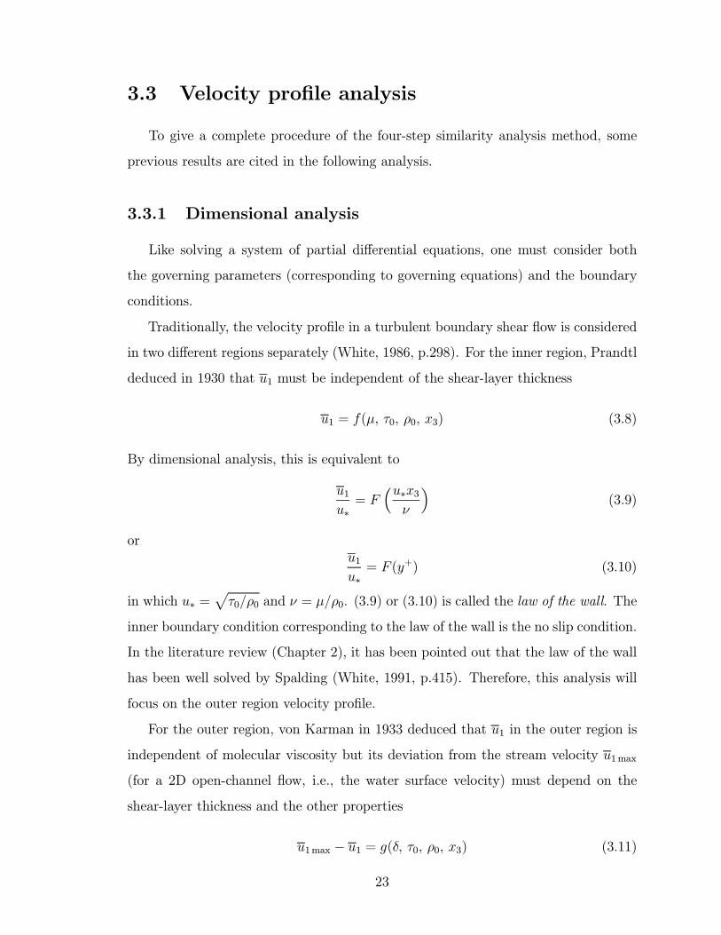
intermediate layer), and wake layer, shown in FIG. 2.1. The velocity proÞle in each
4
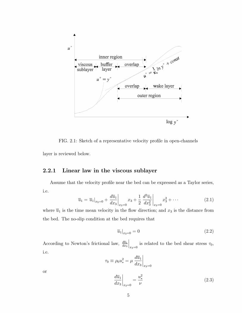
FIG. 2.1: Sketch of a representative velocity proÞle in open-channels
layer is reviewed below.
2.2.1 Linear law in the viscous sublayer
Assume that the velocity proÞle near the bed can be expressed as a Taylor series,
i.e.
u1 = u1|x3=0 +du1dx3
¯x3=0
x3 +1
2
d2u1dx23
¯x3=0
x23 + · · · (2.1)
where u1 is the time mean velocity in the ßow direction; and x3 is the distance from
the bed. The no-slip condition at the bed requires that
u1|x3=0 = 0 (2.2)
According to Newtons frictional law, du1dx3
¯x3=0
is related to the bed shear stress τ0,
i.e.
τ0 ≡ ρ0u2∗ = µdu1dx3
¯x3=0
ordu1dx3
¯x3=0
=u2∗ν
(2.3)
5
in which ρ0 is the water density; u∗ =pτ0/ρ0 is the shear velocity; µ = ρ0ν is the
water dynamic viscosity; and ν is the water kinematic viscosity.
Substituting (2.2) and (2.3) into (2.1) and neglecting the higher order terms yield
the velocity proÞle near the bed as
u1u∗=u∗x3ν
or
u+ = y+ (2.4)
in which u+ = u1/u∗ and y+ = u∗x3/ν are the inner variables. Experiments (Schlicht-
ing, 1979, p.601) show that the above equation is valid in the range of 0 ≤ y+ ≤ 5.The buffer layer velocity proÞle is very complicated and cannot be expressed using
a simple function. It will be discussed in Subsection 2.2.4.
2.2.2 Log law in the overlap
Traditionally, the velocity proÞle in the overlap is expressed by the log law or the
power law. The log law is usually regarded as a complete success since it can be
derived from a complete similarity assumption (Kundu, 1990, p.451), i.e.
u1 =u∗κ0ln x3 + const (2.5)
The above equation is usually expressed in terms of the inner variables as
u+ =1
κ0ln y+ + C1 (2.6)
in which C1 ≈ 5, or in terms of the outer variables asu1max − u1
u∗= − 1
κ0ln ξ + C2 (2.7)
in which u1max = the velocity at the water surface for a wide channel or at the
boundary layer margin for a narrow channel; ξ = x3/δ, and C2 ≈ 1. Experiments
(Kundu, p.453) show that the log law is usually valid in the range of y+ > 30 − 70and ξ < 0.15− 0.2, which is shown in FIG. 2.1.
6
Barenblatt (1996, p.271) has shown that the power law can be derived from an
incomplete similarity assumption and the log law is only a special case of the power
law. Zagarola (1996) experimentally shows that the power law has advantage over
the log law in the range of 50 < y+ < 500. In practice, the log law may still be a
good approximation.
2.2.3 Parabolic law in the wake layer and upper boundary
conditions
The velocity proÞle near a water surface or a boundary layer margin can be
expressed as a Taylor series, i.e.
u1 = u1|ξ=1 +du1dξ
¯ξ=1
(ξ − 1) + 1
2!
d2u1dξ2
¯ξ=1
(ξ − 1)2
+1
3!
d3u1dξ3
¯ξ=1
(ξ − 1)3 + · · · (2.8)
The boundary conditions at the water surface of a 2D channel can be expressed
as:
Velocity at the water surface: u1|ξ=1 = u1max (2.9)
and the shear stress at the water surface (White, 1991, p.149):
τ |ξ=1 = Cdρair(Vwind − u1max)2 (2.10)
in which u1max = the maximum velocity; ρair = 1.21 kg/m3 is the air density in
the standard atmosphere; Vwind is the wind velocity over the water; and Cd = the
water surface drag coefficient which is in the order of 10−3 but difficult to determine
accurately (Roll, 1965, p.160). On the other hand, the shear stress (turbulent shear
stress) at the water surface relates to the velocity gradient by an eddy viscosity, i.e.
τ |ξ=1 = ε+1 ρ0u∗du1dξ
¯ξ=1
(2.11)
in which ε+1 is the dimensionless eddy viscosity at the water surface. From the above
two equations, one derives that
du1dξ
¯ξ=1
=Cdρair(Vwind − u1max)2
ε+1 ρ0u∗
7
= λ0(Vwind − u1max)2
u∗(2.12)
in which λ0 = Cdρair/(ε+1 ρ0) is called the water surface shear effect factor. The above
equation shows that the shear stress at the water surface is usually nonzero except
that the wind velocity over the water is equal to the water surface velocity.
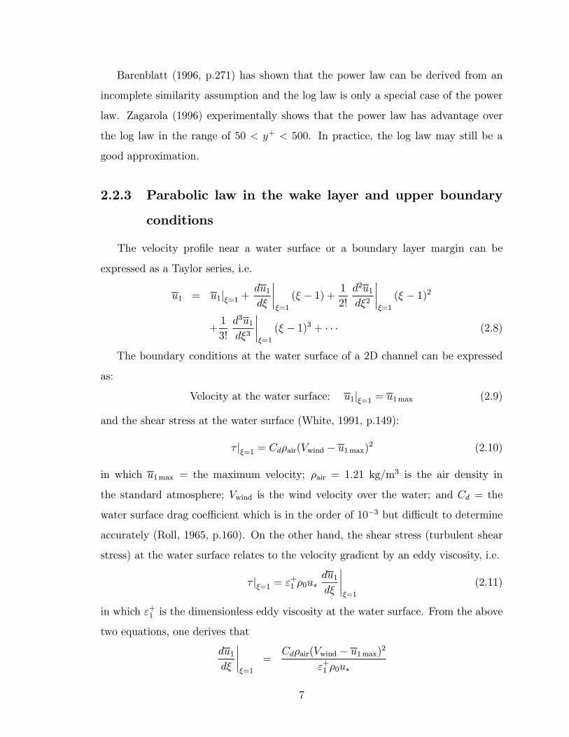
However, the boundary layer thickness in a narrow channel is not the water depth,
rather it is usually deÞned as the distance from the bed to the maximum velocity
position. In this case, the velocity gradient at the maximum velocity must be zero,
i.e.du1dξ
¯ξ=1
= 0 (2.13)
The above condition is also required in a circular pipe ßow. (2.13) may also be
expressed by (2.12) except that λ0 = 0. (2.13) and (2.12) are shown in FIG. 2.2.
Now neglecting the 3rd and higher order terms in (2.8), one obtains
u1 = u1max +du1dξ
¯ξ=1
(ξ − 1) + 1
2!
d2u1dξ2
¯ξ=1
(ξ − 1)2 (2.14)
oru1u∗=u1maxu∗
+1
u∗
du1dξ
¯ξ=1
(ξ − 1) + 1
2!
1
u∗
d2u1dξ2
¯ξ=1
(ξ − 1)2 (2.15)
The above equation can be rewritten as a defect form:
u1max − u1u∗
=1
u∗
du1dξ
¯ξ=1
(1− ξ)− 1
2!
1
u∗
d2u1dξ2
¯ξ=1
(1− ξ)2 (2.16)
in which du1dξ
¯ξ=1
is deÞned by (2.12) or (2.13); and 12u∗
d2u1dξ2
¯ξ=1
is determined experi-
mentally.
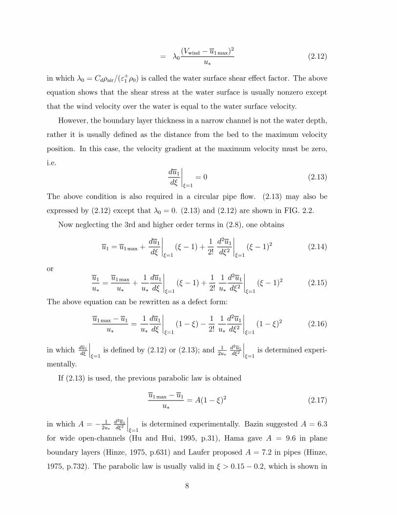
If (2.13) is used, the previous parabolic law is obtained
u1max − u1u∗
= A(1− ξ)2 (2.17)
in which A = − 12u∗
d2u1dξ2
¯ξ=1
is determined experimentally. Bazin suggested A = 6.3
for wide open-channels (Hu and Hui, 1995, p.31), Hama gave A = 9.6 in plane
boundary layers (Hinze, 1975, p.631) and Laufer proposed A = 7.2 in pipes (Hinze,
1975, p.732). The parabolic law is usually valid in ξ > 0.15− 0.2, which is shown in
8
FIG. 2.2: Upper derivative boundary conditions in pipes, narrow channels (a/h < 5),
and wide channels (a/h ≥ 5)
9
Log overlap Parabolic law
10-2 10-1 1000
2
4
6
8
10
12
14 // / / / / / / / / / / / / / / / / / / / / / / / / / / / / / / / / / / / / / / / / / / / / / / / / / / / / / / / / / / / / / / / / / / / / / / / / / / / / / / / / / / / / / / / / / / / / / / / / / /
////// Area of experimental data
ξ = x3/δ
u 3m
ax-u
3
u *__
____
_
FIG. 2.3: The velocity defect law in the outer region (After Hinze, 1975, p.631)
FIG. 2.3. However, the velocity gradient at the water surface in a wide channel is not
necessary to be zero, as indicated in (2.12).
Equations (2.4), (2.7) and (2.16) are independent of any turbulent models and
are indeed three physical constraints to the velocity proÞle. A satisfactory turbulent
model must meet them simultaneously. In practice, the viscous and the buffer layers
may be neglected, in particular in a rough boundary. Therefore, (2.7) and (2.16) must
be at least met.
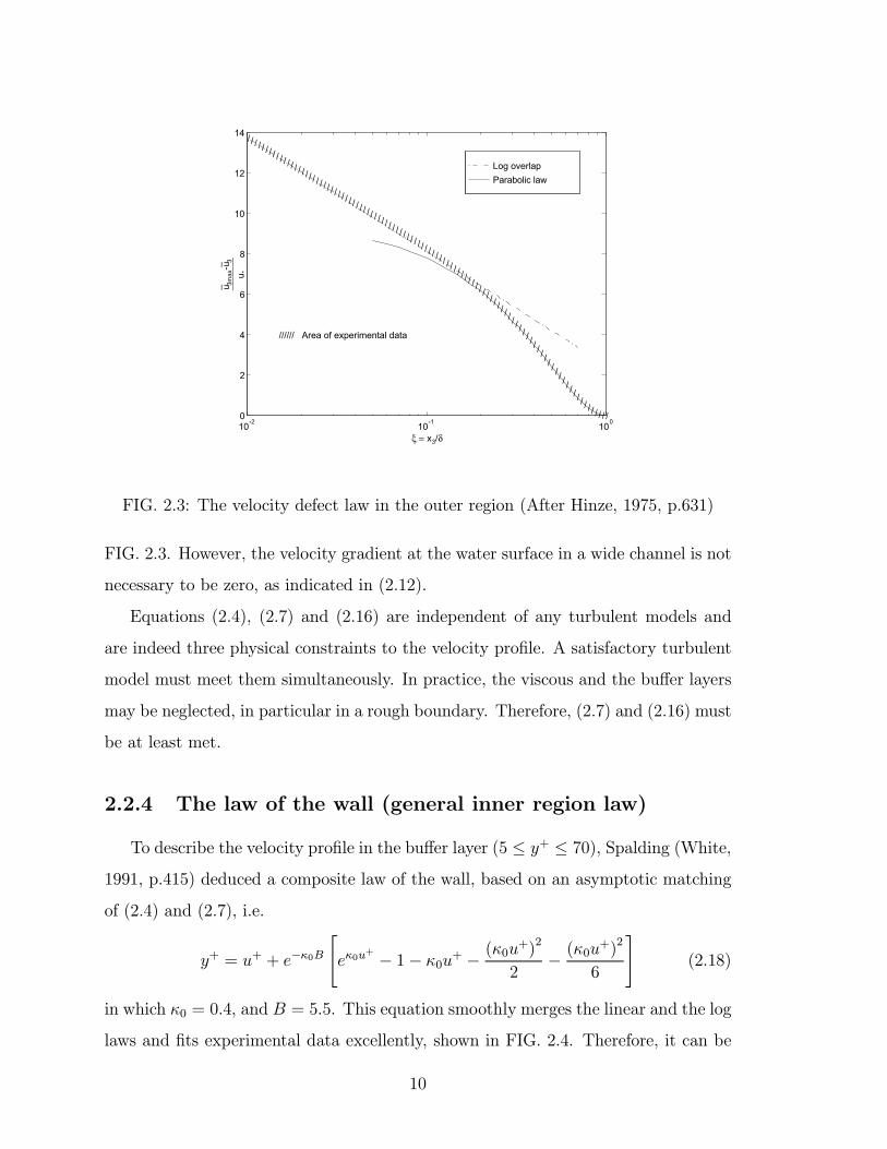
2.2.4 The law of the wall (general inner region law)
To describe the velocity proÞle in the buffer layer (5 ≤ y+ ≤ 70), Spalding (White,1991, p.415) deduced a composite law of the wall, based on an asymptotic matching
of (2.4) and (2.7), i.e.
y+ = u+ + e−κ0B"eκ0u
+ − 1− κ0u+ − (κ0u+)2
2− (κ0u
+)2
6
#(2.18)
in which κ0 = 0.4, and B = 5.5. This equation smoothly merges the linear and the log
laws and Þts experimental data excellently, shown in FIG. 2.4. Therefore, it can be
10
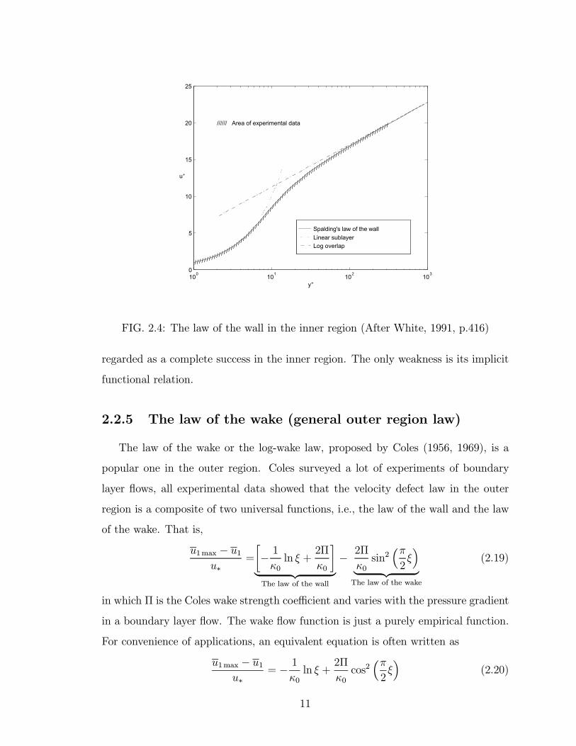
Spalding's law of the wallLinear sublayer Log overlap
100 101 102 1030
5
10
15
20
25
/ / / / / / // / / /
/ / / // / /
/ / // /
/ // /
/ // /
/ // /
/ // /
/ // / /
/ / // / /
/ / // / /
/ / // / /
/ / // / /
/ / // / /
/ / // / /
////// Area of experimental data
y+
u+
FIG. 2.4: The law of the wall in the inner region (After White, 1991, p.416)
regarded as a complete success in the inner region. The only weakness is its implicit
functional relation.
2.2.5 The law of the wake (general outer region law)
The law of the wake or the log-wake law, proposed by Coles (1956, 1969), is a
popular one in the outer region. Coles surveyed a lot of experiments of boundary
layer ßows, all experimental data showed that the velocity defect law in the outer
region is a composite of two universal functions, i.e., the law of the wall and the law
of the wake. That is,
u1max − u1u∗
=
·− 1κ0ln ξ +
2Π
κ0
¸| z The law of the wall
− 2Π
κ0sin2
³π2ξ´
| z The law of the wake
(2.19)
in which Π is the Coles wake strength coefficient and varies with the pressure gradient
in a boundary layer ßow. The wake ßow function is just a purely empirical function.
For convenience of applications, an equivalent equation is often written as
u1max − u1u∗
= − 1κ0ln ξ +
2Π
κ0cos2
³π2ξ´
(2.20)
11
Several hydraulicians (Coleman, 1981, 1986; Nezu and Nakagawa, 1993) system-
atically examined it in open-channels. They found that the wake ßow function can
also improve the accuracy of velocity proÞles in open-channels. For clear water, the
Coles wake strength coefficient Π is about 0 − 0.2. Note that although many inves-tigators regarded the log-wake law as a great success in the outer region, as Coles
(1969) stated, it is not valid near the upper boundary layer edge (ξ > 0.6−0.9). Thisis because it does not satisfy the boundary condition (2.12) or (2.13).
In summary, no existing velocity proÞle equation satisÞes (2.12) or (2.13).
2.3 Velocity ProÞles in Sediment-Laden Flows
Because more independent variables, such as sediment concentration and density
gradient, are involved in sediment-laden ßow systems, velocity proÞles in sediment-
laden ßows are much more complicated than those in clear water. In this section, only
the applications of the log law and the log-wake law will be reviewed. The application
of the power law is neglected here although several studies have been reported.
2.3.1 Extension of the log law to sediment-laden ßows
Vanoni (1946), Einstein and Chien (1955), Vanoni and Nomicos (1960), Elata
and Ippen (1961), and many others examined the log law in sediment-laden ßows
experimentally. They concluded that the log law remains valid except that κ, which is
the von Karman constant in sediment-laden ßow, decreases with sediment suspension.
Furthermore, Einstein and Chien (1955) proposed a graphical relation to predict the
von Karman constant κ based on an energy concept, as shown in FIG. 2.5. They also
pointed out that the main effect of sediment suspension occurs near the bed.
Later, Vanoni and Nomicos (1960) modiÞed the Einstein and Chien parameter
with the average volumetric concentration near the bed. Barton and Lin (1955) dis-
cussed the variation of the von Karman constant κ from the view of density gradient.
Chien and Wan (1983, p.396) uniÞed various arguments with a Richardson number.
However, their study could not explain Elata and Ippens (1961) neutral particle ex-
12
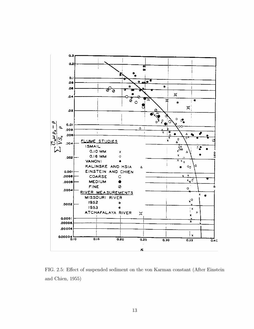
FIG. 2.5: Effect of suspended sediment on the von Karman constant (After Einstein
and Chien, 1955)
13
periments. To explain his neutral particle experiments, Ippen (1971) argued that
suspended sediment affects the velocity proÞle mainly by changing water viscosity. A
good summary of this type of research can be found in the literature (Vanoni, 1975,
p.83-91; Chien and Wan, 1983, p.391-401; Hu and Hui, 1995, p.130-137).
Almost at the same time as Einstein and Chien (1955), Kolmogorov (1954) and
Barenblatt (1953, 1996) also analyzed the effect of sediment suspension on the log
law from a view of complete similarity. They considered the momentum equation, the
sediment concentration equation and the turbulent energy equation simultaneously
and concluded that the log law is still valid in sediment-laden ßows except that the
von Karman constant becomes smaller. This is exactly the same conclusion as that
drawn by Einstein and Chien (1955). Barenblatt (1996, p.270) further pointed out
that the application of the log law in sediment-laden ßows, as it in clear water, is
limited to the overlap zone. In other words, the log law may not be valid in the wake
layer and near the water surface.
2.3.2 Extension of the log-wake law to sediment-laden ßows
Coleman (1981, 1986) introduced the log-wake law to open channels and studied
the effect of suspended sediment on the parameters κ and Π. He argued that if
the log-wake law is applied, the von Karman constant κ remains the same as that
in clear water κ0, but the wake strength coefficient Π increases with a Richardson
number, shown in FIG. 2.6. He further pointed out that the previous conclusion, i.e.,
κ decreases with sediment suspension, was obtained by incorrectly extending the log
law to the wake layer.
Colemans argument was supported by Parker and Coleman (1986), Cioffi and
Gallerano (1991). A similar result was obtained at CSU by Janin (1986) in a large
boundary layer wind tunnel. Colemans conclusion is actually an analogy to the ef-
fect of pressure-gradient on boundary-layer ßows. However, the pressure equation of a
boundary layer ßow in the normal direction is not similar to the sediment concentra-
tion equation in a sediment-laden ßow. The pressure or pressure-gradient is regarded
as a constant at a certain cross-section in a boundary layer ßow while the sediment
14
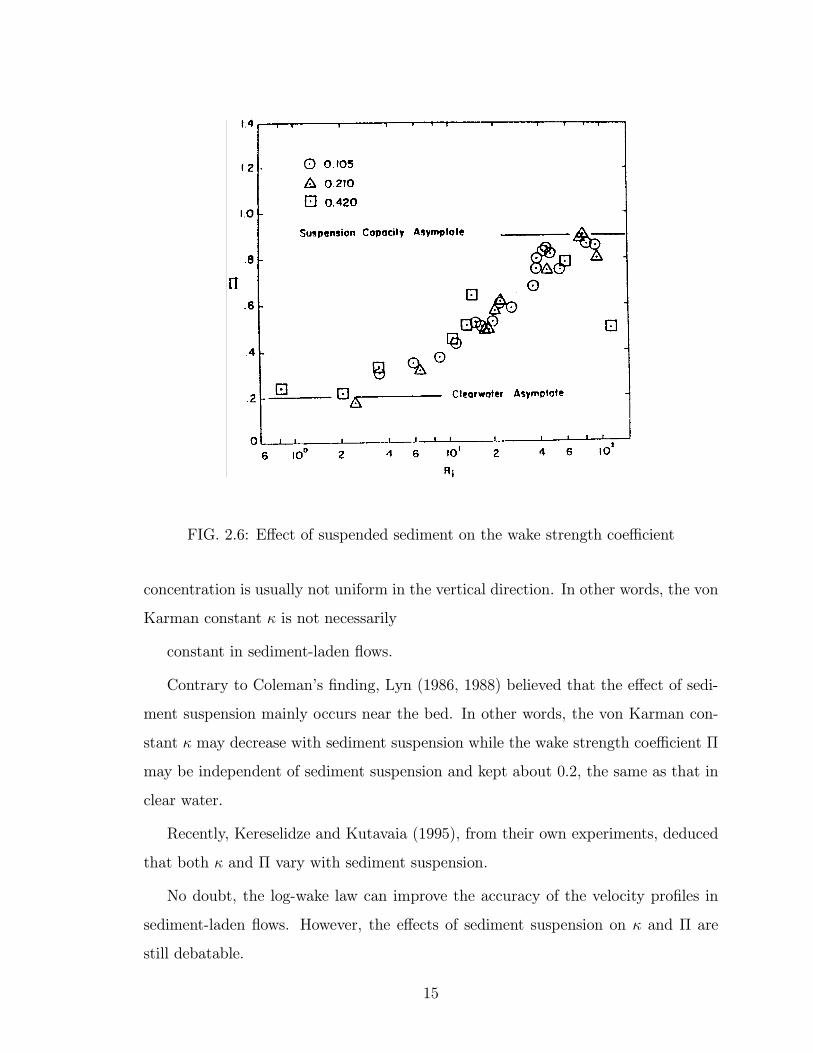
FIG. 2.6: Effect of suspended sediment on the wake strength coefficient
concentration is usually not uniform in the vertical direction. In other words, the von
Karman constant κ is not necessarily
constant in sediment-laden ßows.
Contrary to Colemans Þnding, Lyn (1986, 1988) believed that the effect of sedi-
ment suspension mainly occurs near the bed. In other words, the von Karman con-
stant κ may decrease with sediment suspension while the wake strength coefficient Π
may be independent of sediment suspension and kept about 0.2, the same as that in
clear water.
Recently, Kereselidze and Kutavaia (1995), from their own experiments, deduced
that both κ and Π vary with sediment suspension.
No doubt, the log-wake law can improve the accuracy of the velocity proÞles in
sediment-laden ßows. However, the effects of sediment suspension on κ and Π are
still debatable.
15
2.3.3 Log-linear law and others
The log-linear law was originally proposed in temperature stratiÞed ßows (Kundu,
1990, p.463). It is written as
u1u∗=1
κ
·lnx3x30
+ 5x3LM
¸(2.21)
in which x30 is a reference point; and LM is the Monin-Obukhov length. The above
equation can be written as a defect form as follows:
u1max − u1u∗
=1
κ
·− ln x3
δ+ 5
δ − x3LM
¸= −1
κln ξ +
5
κ
δ
LM(1− ξ) (2.22)
in which ξ = x3/δ. From the formula appearance, the log-linear law is another type
of the log-wake law, except that the wake function is a linear function rather than
a sine function. However, from its derivation (Duo, 1987, p.365), the log-linear law,
like the log law, is only valid in the overlap since it is assumed that the shear stress is
a constant. In addition, the above log-linear law is derived under the assumption of
small values of Richardson number Ri (Roll, 1965, p.147). In other words, one cannot
expect that it will prove useful under conditions of great density gradient ßows.
Itakura and Kishi (1980) and McCutcheon (1981) applied the log-linear law to
sediment-laden ßows. However, this extension is not accepted by sediment researchers.
As pointed out by Lyn (1986), the foundation of the log-linear law, where the tur-
bulent temperature ßux is a constant, is not applicable in sediment-laden ßows since
the turbulent sediment concentration ßux is not a constant in the vertical direction at
all. Although the log-linear law is not applicable in sediment-laden ßows theoretically,
the comparison of the log-linear law with experimental data (Itakura and Kishi,1980;
McCutcheon, 1981) looks very good.
Besides the log-wake law and the log-linear law, some other wake function forms
can be found in literature. Ni and Hui (1988) proposed a wake ßow function with two
terms: one indicates the effect of mean concentration; the other expresses the effect
of concentration gradient. Umeyama and Gerritsen (1992) and Zhou and Ni (1995)
16
suggested a Taylor series to express the wake ßow function. In addition, the study
of the power law was reported by Chien and Wan (1983), Chen (1984), Karim and
Kennedy (1987) and Woo, Julien and Richardson (1988).
2.4 Summary
No existing (outer region) velocity proÞle laws in clear water are fully satisfactory.
The log law is valid only in the overlap. The log-wake law does not satisfy the upper
boundary condition. The parabolic law is only valid near the water surface in narrow
channels. The log-linear law is good in temperature stratiÞed ßows, but the foun-
dation of its assumptions may not applicable in sediment-laden ßows. Consequently,
the applications of these laws in sediment-laden ßows are not satisfactory.
17
Chapter 3
SIMILARITY ANALYSIS OF
CLEAR WATER VELOCITY
PROFILES
3.1 Introduction
Turbulence is complicated. Although the governing Navier-Stokes equations have
been established over a century, no solutions for turbulent ßows (high Reynolds num-
ber ßows) are yet available, even for a simple steady uniform 2D turbulence. To Þnd
a time-averaged solution of turbulence, the Reynolds averaged equations are usually
applied. However, the average process brings new unknowns to the ßow system. In
other words, the Reynolds equations are not closed and cannot be solved theoreti-
cally. Dimensional analysis or similarity analysis is usually helpful in such a case. The
new difficulty from the classical dimensional analysis is that it only gives similarity
parameters. It cannot give the speciÞc functional relations.
Recently, Barenblatt (1996) has extended the dimensional analysis method. In
particular, the concept of the intermediate asymptotics suggested by him is very
powerful in a turbulence analysis. Based on previous studies, an improved similarity
analysis approach is Þrst presented in Section 3.2. Then its application in the study
18
of clear water velocity proÞle is discussed in Section 3.3. An eddy viscosity, based on
the new velocity proÞle law, is discussed in Section 3.4. Section 3.5 brießy summaries
the results of this chapter.
3.2 Four-step similarity analysis method
Suppose there is a physical system including a turbulent ßow in a 2D pipe or
open-channel. The governing equations of the system are not closed, unknown, or
too difficult to solve. One may proceed with a similarity analysis in the following
way: dimensional analysis, intermediate asymptotics, wake correction, and boundary
correction. These four steps are referred to as the four-step similarity analysis method.
The following is the discussion of each step.
3.2.1 Dimensional analysis
For simplicity, one assumes an equilibrium physical system. The dimensional
analysis includes: (a) specifying governing parameters (independent and dependent
parameters) and their dimensions; (b) specifying the boundary conditions; (c) choos-
ing the repeated parameters; and (d) using Buckinghams Π theorem to normalize
the governing parameters and the boundary conditions with the repeated parameters
and putting the function under study into a dimensionless form, i.e.
The governing parameters
Π = Φ(Π1, Π2, · · · , Πm) (3.1)
The boundary conditions
limx→Γ
Π = φ, limx→Γ
∂Π
∂Πj= φ1, lim
x→Γ∂2Π
∂Π2j= φ2, · · · (3.2)
in which Π is the dependent similarity parameter; Π1, Π2, · · ·, and Πm are independentsimilarity parameters; x → Γ denotes the space variable tends to the boundary; φ
denotes the boundary values; and subscripts 1 and 2 denote the values of the Þrst
and the second derivatives; and j = 1, 2, · · · ,m. (3.1) is equivalent to the governing
19
equations which may be a vector. The number of the boundary conditions depends
on the governing equations (ODE or PDE). However, if the governing equations are
unknown, try to write as many conditions as possible. (3.2) are constraints of (3.1).
3.2.2 Intermediate asymptotics
According to Barenblatt (1996, p. xiii), the intermediate asymptotics means that
for a certain governing similarity parameter, its value is intermediate, i.e., neither
too big nor too small. For a time-dependent problem, the intermediate asymptotics
means that the system is independent of the Þne details of the initial conditions and
also far away from the equilibrium state. For an equilibrium problem, the physical
domain considered is far away from the boundary. In other words, the dependent
parameters under consideration are independent of the boundary conditions. The
intermediate asymptotics usually includes two steps: one is the test of complete
similarity assumption, and the other is the test of incomplete similarity assump-
tion.
Complete similarity: If the system is completely independent of a certain para-
meter, say, Πm, one says that the system is complete similarity with respect to Πm.
Then Πm disappears in (3.1), the number of the independent parameters reduces to
m− 1.Incomplete similarity: Suppose that Φ tends to zero or inÞnity when Πm goes to
zero or inÞnity. This means that the quantity of Πm remains essential in the system,
and (3.1) may be rewritten as (Barenblatt, 1996, p. 24, p. 145, Chap. 5):
Π = Πα1mΦ
µΠ1Πα2m
,Π2Πα3m
, · · · , Πm−1Παmm
¶(3.3)
in which the exponents α1, α2, · · ·, and αm must be determined experimentally. Thiskind of similarity is called incomplete similarity.
3.2.3 Wake correction (or wake function)
From its deÞnition, the intermediate asymptotics is not valid beyond the corre-
sponding intermediate domain. The deviation between the real values of Π and the
20
intermediate asymptotics beyond the intermediate domain is called the wake cor-
rection or wake function W . This is analogous to the Coles wake ßow function in
turbulent boundary layers (Coles, 1956). Now one has
Π = Φ(Π1, Π2, · · · , Πm−1) +W (Π1, Π2, · · · , Πm) (3.4)
for a complete similarity, and
Π = Πα1mΦ
µΠ1Πα2m
,Π2Πα3m
, · · · , Πm−1Παmm
¶+W (Π1, Π2, · · · , Πm) (3.5)
for an incomplete similarity. Obviously, the wake correction must be very small
compared with the Þrst term when Πm goes to its intermediate values.
3.2.4 Boundary correction
Equation (3.4) or (3.5) has extended the solution near the boundary. However,
the boundary conditions are usually not satisÞed. To meet the boundary condition,
another additional term which is called the boundary correction B may be added to
(3.4) and (3.5). Then one has
Π =Φ(Π1, Π2, · · · , Πm−1)| z Intermediate asymptotics
+ W (Π1, Π2, · · · , Πm)| z Wake correction
+ B(Π1, Π2, · · · , Πm)| z Boundary correction
(3.6)
or
Π =Πα1mΦ
µΠ1Πα2m
,Π2Πα3m
, · · · , Πm−1Παmm
¶| z
Intermediate asymptotics
+ W (Π1, Π2, · · · , Πm)| z Wake correction
+ B(Π1, Π2, · · · , Πm)| z Boundary correction
(3.7)
The boundary correction function B is usually a polynomial. The power of the polyno-
mial is equal to the highest order of derivative boundary condition. For example, if the
highest order of the derivative boundary condition is a Þrst order, then the boundary
correction function B will be a linear function. The function B can be determined by
expanding the Þrst two terms at the boundary. The detailed method for determining
the boundary correction function B will be illustrated in the following section.
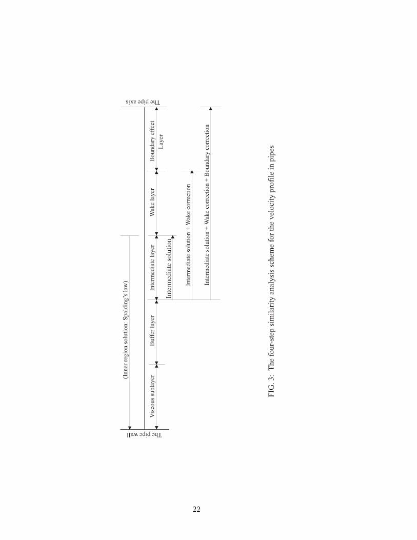
One can see that a similarity solution may consist of three parts: intermediate
asymptotics, wake correction, and boundary correction. Take the velocity proÞle in
a pipe ßow as an example, the above four steps can be summarized in FIG. 3.1.
21
22
3.3 Velocity proÞle analysis
To give a complete procedure of the four-step similarity analysis method, some
previous results are cited in the following analysis.
3.3.1 Dimensional analysis
Like solving a system of partial differential equations, one must consider both
the governing parameters (corresponding to governing equations) and the boundary
conditions.
Traditionally, the velocity proÞle in a turbulent boundary shear ßow is considered
in two different regions separately (White, 1986, p.298). For the inner region, Prandtl
deduced in 1930 that u1 must be independent of the shear-layer thickness
u1 = f(µ, τ0, ρ0, x3) (3.8)
By dimensional analysis, this is equivalent to
u1u∗= F
³u∗x3ν
´(3.9)
oru1u∗= F (y+) (3.10)
in which u∗ =pτ0/ρ0 and ν = µ/ρ0. (3.9) or (3.10) is called the law of the wall. The
inner boundary condition corresponding to the law of the wall is the no slip condition.
In the literature review (Chapter 2), it has been pointed out that the law of the wall
has been well solved by Spalding (White, 1991, p.415). Therefore, this analysis will
focus on the outer region velocity proÞle.
For the outer region, von Karman in 1933 deduced that u1 in the outer region is
independent of molecular viscosity but its deviation from the stream velocity u1max
(for a 2D open-channel ßow, i.e., the water surface velocity) must depend on the
shear-layer thickness and the other properties
u1max − u1 = g(δ, τ0, ρ0, x3) (3.11)
23
Again, by dimensional analysis one writes this as
u1max − u1u∗
= G³x3δ
´(3.12)
oru1max − u1
u∗= G(ξ) (3.13)
in which ξ = x3/δ. (3.12) or (3.13) is called the velocity defect law. The boundary
conditions corresponding to the defect law should be (2.9) and (2.12) or (2.13). They
will be met by choosing the function G.
3.3.2 Intermediate asymptotics
Assume that the channel bed corresponds to the boundary Γ1 and the upper
boundary (the maximum velocity in a narrow channel or the water surface in a wide
channel) corresponds to the boundary Γ2 in FIG. 3.1. Then the left part corresponds
to the inner region in a channel ßow while the right part corresponds to the outer
region. Obviously, unlike previous studies, the outer region is now divided into three
layers: the overlap, the wake layer, and the boundary effect layer. The boundary
effect layer is emphasized here.
From FIG. 3.1, the intermediate layer or overlap belongs to both the inner region
and the outer region. Then both (3.10) and (3.13) are valid in the overlap. From
(3.10) one gets the velocity gradient as (Millikan, 1938; Kundu, 1990, p.452)
du1dx3
=u2∗ν
dF
dy+(3.14)
From (3.13) one hasdu1dx3
=u∗δ
dG
dξ(3.15)
Equating (3.14) and (3.15) and multiplying by x3/u∗, one has
ξdG
dξ= y+
dF
dy+=1
κ0(3.16)
which is valid for large y+ and small ξ. Since the left side is only a function of ξ and
the right side is only a function of y+, both sides must be equal to the same universal
24
constant, say 1/κ0, where κ0 is the von Karman constant in clear water. Integration
of (3.16) gives
F (y+) =1
κ0ln y+ + C1 (3.17)
and
G(ξ) =1
κ0ln ξ + C2 (3.18)
in which κ0, C1 and C2 are experimental constants. The above log law is actually
derived on the assumption of complete similarity with respect to Reynolds number
in the intermediate region.
Barenblatt (1996, p.269) showed that under the assumption of incomplete similar-
ity with Reynolds number, a power law in the intermediate region may be obtained.
This study will concentrate on the log law. The brief study of a power law, under the
assumption of incomplete similarity, in pipe ßows is appended in Appendix A.
3.3.3 Wake correction to the log law
Based on (3.17), Coles (1956, 1969) analyzed a lot of experimental proÞles and
determined that the wake correction can be well approximated as
W (ξ) = Ω0 sin2 πξ
2(3.19)
in which Ω0 is the wake value at ξ = 1. In other words, the log law may be extended
to the wake layer by adding the wake function (3.19) to (3.17), i.e.
u1u∗=1
κ0ln y+ + C1 + Ω0 sin
2 πξ
2(3.20)
Considering y+ = Re∗ξ, in which the Reynolds number Re∗ = u∗δ/ν, the above
equation can be rewritten by the outer variable ξ, i.e.
u1u∗=1
κ0ln ξ + C3 + Ω0 sin
2 πξ
2(3.21)
in which C3 = 1/κ0 lnRe∗ + C1. This is just the log-wake law proposed by Coles
(1956). As Coles (1969) stated later, this law is not valid near the upper boundary
layer since the derivative boundary condition at the boundary edge is not satisÞed.
25
3.3.4 Boundary correction to the log-wake law
According to (3.6), assume a boundary correction function B(ξ), then (3.21) be-
comesu1u∗=1
κ0ln ξ + C3 + Ω0 sin
2 πξ
2+B(ξ) (3.22)
in which B(ξ) is a linear function since the highest derivative boundary condition is
a Þrst order derivative.
One can expand the above equation at ξ = 1. One has
ln ξ = ln[1− (1− ξ)] = −∞Xi=1
(1− ξ)ii
= −(1− ξ)− (1− ξ)2
2− · · · (3.23)
sin2π
2ξ =
1− cosπξ2
=1
2+cos(π − πξ)
2
= 1− 12
∞Xi=1
(−1)i [π(1− ξ)]2i
(2i)!
= 1− π2
4(1− ξ)2 + · · · (3.24)
and
cos2π
2ξ =
π2
4(1− ξ)2 + · · · (3.25)
(3.25) will be used later. Now substituting (3.23) and (3.24) into (3.21) and neglecting
the 3rd and higher order terms yield that
u1u∗
= −1− ξκ0
− (1− ξ)2
2κ0+ C3 + Ω0
µ1− π
2
4(1− ξ)2
¶+B(ξ)
= (C3 + Ω0)− 1− ξκ0
−µ1
2κ0+π2
4Ω0
¶(1− ξ)2 +B(ξ) (3.26)
It is assumed that B(ξ) is linear, comparing (3.26) and (2.15), one has
C3 + Ω0 =u1maxu∗
(3.27)
B(ξ) =
"1
κ0− 1
u∗
du1dξ
¯ξ=1
#(1− ξ) (3.28)
26
Finally, the log-wake law is modiÞed as
u1u∗=1
κ0ln ξ +
u1maxu∗
−Ω0 cos2 πξ2+
"1
κ0− 1
u∗
du1dξ
¯ξ=1
#(1− ξ) (3.29)
which can be rewritten as a velocity defect form
u1max − u1u∗
= − 1κ0ln ξ + Ω0 cos
2 πξ
2−"1
κ0− 1
u∗
du1dξ
¯ξ=1
#(1− ξ) (3.30)
in which κ0 and Ω0 are two experimental constants. This is the Þnal velocity proÞle
equation based on the log law, which is called the modiÞed log-wake law. The last
term is due to the boundary correction which is a main contribution of this study.
Considering (2.12) and (2.13), (3.30) may further be written as
u1max − u1u∗
= − 1κ0ln ξ + Ω0 cos
2 πξ
2−"1
κ0− λ0
µVwind − u1max
u∗
¶2#(1− ξ)
(3.31)
in which λ0 = 0 for narrow channels and pipes, and λ0 > 0 for wide channels.
3.4 Implication to turbulent eddy viscosity
The eddy viscosity is not a measurable variable. It is usually derived from some
assumptions, such as the mixing length hypothesis, or from the mean velocity proÞles
for simple ßows. If (3.30) is correct, an eddy viscosity model can be deduced.
Assume that the shear stress is linearly distributed along the ßow depth and the
viscous shear stress can be neglected, the distribution of the eddy viscosity ε may be
derived from
ε =τ0ρ
(1− ξ) + τ |ξ=1 /τ01
δ
du1dξ
= δu∗(1− ξ) + τ |ξ=1 /τ0
1
u∗
du1dξ
or
ε+ ≡ ε
δu∗=(1− ξ) + τ |ξ=1 /τ0
1
u∗
du1dξ
(3.32)
27
in which τ |ξ=1 is the shear stress on the water surface; and ε+ is deÞned as thedimensionless eddy viscosity.
From (3.30), one has
1
u∗
du1dξ
=1− ξκ0ξ
+πΩ02sinπξ +
1
u∗
du1dξ
¯ξ=1
Substituting the above equation into (3.32) gives
ε+ =(1− ξ) + τ |ξ=1 /τ0
1− ξκ0ξ
+πΩ02sin πξ +
1
u∗
du1dξ
¯ξ=1
(3.33)
which is the eddy viscosity model corresponding to the modiÞed log-wake law. The
shear stress and the velocity gradient at the water surface are boundary conditions.
When ξ → 0, (3.33) tends to
ε+ → κ0ξ (3.34)
which is the classical mixing length model. When ξ → 1, (3.33) tends to
ε+ → τ |ξ=1 /τ01
u∗
du1dξ
¯ξ=1
= const (3.35)
which corresponds to the constant eddy viscosity model.
(3.33) along with (3.30) will be examined with experimental data later.
3.5 Summary
In this chapter, an improved similarity analysis approach, the four-step similar-
ity analysis method, is presented, which includes dimensional analysis, intermediate
asymptotics, wake correction, and boundary correction. Based on this approach, the
modiÞed log-wake law is proposed, which is expressed in (3.30) or (3.31). The modiÞed
log-wake law satisÞes the upper boundary conditions. Furthermore, an eddy viscosity
model is deduced.
28
Chapter 4
SHEAR VELOCITY IN SMOOTH
OPEN-CHANNELS
4.1 Introduction
One may skip this chapter if he simply accepts (4.16) and (4.23) as the equations
to estimate the centerline bed shear velocity in a rectangular channel. (4.16) is for the
aspect ratio a/h > 2.5 while (4.23) is for the aspect ratio a/h ≤ 2.5. After reading thisdissertation, if interested, one may come back to enjoy this mathematical derivation.
The shear velocity u∗, as a boundary condition, is a prerequisite in the study of
velocity proÞles. Conventionally, four methods for determining u∗ can be found in the
literature (Muste and Patel, 1997; Nezu, Kadita and Nakagawa, 1997): (1) from the
shear stress distribution; (2) from the log law; (3) using a global shear velocity based
on the hydraulic radius; and (4) using the shear velocity based on the ßow depth. The
Þrst two methods must be aided with experimental data and are cumbersome. The
third one is just a global value of u∗ while the shear velocity in the velocity proÞle
should be the local value. The last one is useful for a wide channel. However, most
laboratory ßume experiments belong to narrow channel ßows. Recently, Yang and
Lim (1997) presented a method for calculating the shear velocity in smooth open-
channels, based on an energy dissipation assumption. The method is excellent for the
estimation of the average bed shear velocity, but the calculation of the local shear
29
velocity is still open. Besides, the equation is implicit and the calculation requires
an iterative process. Obviously, the determination of the shear velocity in an open-
channel is very difficult.
This study will begin with a conformal mapping of a rectangular cross-section into
a half-up plane (Section 4.2). Then the bed shear stress distribution (Section 4.3)
and the average bed shear stress (Section 4.4) will be derived. Section 4.5 summaries
the results of this chapter.
4.2 Conformal mapping from a rectangular cross-
section (z-plane) into a half upper plane (w-
plane)
Because of secondary ßows and nonuniform roughness distribution around the
wetted perimeter, it is impossible to get an exact solution for the boundary shear
stress distribution. To obtain an approximate solution, the following assumptions are
made: (1) the boundary is smooth; and (2) the velocity contours are parallel to the
boundary. That is, the boundary is a velocity contour and there are no secondary
ßows in the channel. The Þrst assumption can be met in most ßume experiments.
The second assumption is apparently not true, it will be considered in the solution
by introducing a correction factor.
Based on the above assumptions, the Schwartz-Christoffel transformation (Spiegel,
1993, p.206) can be used to Þnd the isovels (velocity contours, which are parallel to
the boundary) and the rays (curves which are perpendicular to the isovels and the
boundary). Considering a rectangular cross-section with width a and ßow depth h and
using the Schwartz-Christoffel transformation, one can map the physical ßow domain
(z−plane) into a half-upper plane (w−plane), shown in FIG. 4.1. The transformationrelation between them is
w =a
πsinπz
a(4.1)
30
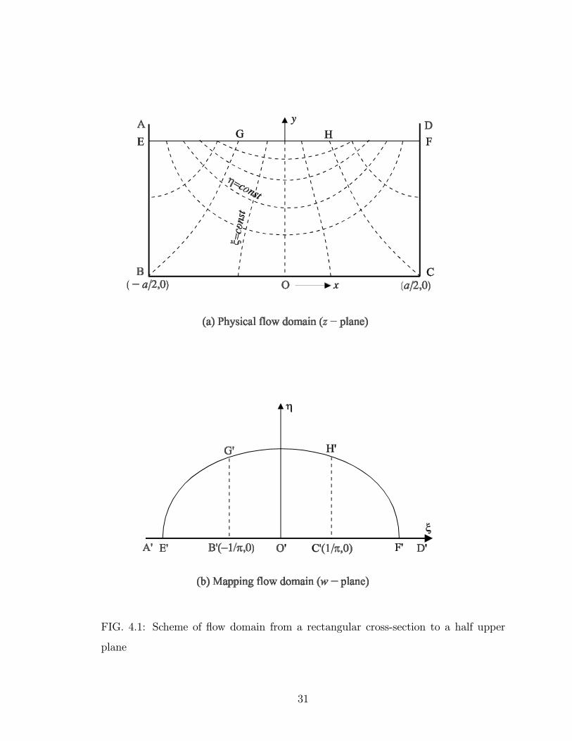
FIG. 4.1: Scheme of ßow domain from a rectangular cross-section to a half upper
plane
31
in which a is the channel width, and
z = x+ iy (4.2)
w = ξ + iη (4.3)
Relation (4.1) can be found in many text books of complex variables (for example,
Spiegel, 1993, p.206).
Substituting (4.2) and (4.3) into (4.1), one has
ξ + iη =a
πsinπ
a(x+ iy)
=a
π
³sinπx
acosh
πy
a+ i cos
πx
asinh
πy
a
´or
ξ =a
πsinπx
acosh
πy
a(4.4)
η =a
πcos
πx
asinh
πy
a(4.5)
ξ = const in (4.4) is a ray equation. Similarly, η = const in (4.5) is an isovel equation,
shown in FIG. 4.1(a).
Since the water surface in the z−plane is described by the equation y = h, whereh is the ßow depth. Substituting this relation into (4.4) and (4.5) gives the water
surface mapping E0G0H 0F 0 in the w−plane, which is a half upper ellipse, as shownin FIG. 4.1(b). The problem is usually solved in the w−plane. In this case, however,one just goes back to the physical plane (z−plane) with the transformations (4.4)and (4.5).
4.3 Bed shear stress distribution and centerline
shear velocity
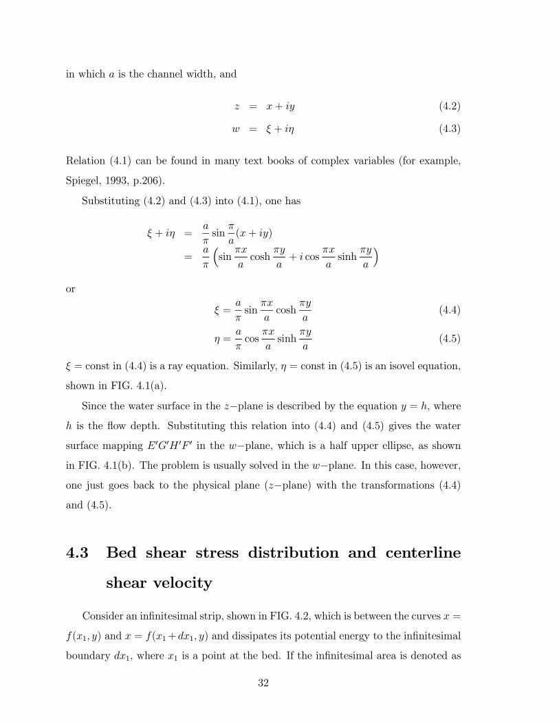
Consider an inÞnitesimal strip, shown in FIG. 4.2, which is between the curves x =
f(x1, y) and x = f(x1+dx1, y) and dissipates its potential energy to the inÞnitesimal
boundary dx1, where x1 is a point at the bed. If the inÞnitesimal area is denoted as
32
FIG. 4.2: Scheme for computing bed shear stress distribution
dAb, considering the equilibrium between the gravity component of the strip in the
ßow direction and the bed shear force in dx1 gives
ρ0gSdAb = τbdx1 (4.6)
in which τb is the local bed shear stress. It is noted again that since x = f(x1, y) is
perpendicular to isovels, there is no shear stress between the strip and its neighbor
ßuid.
Equation (4.6) gives
τb = ρ0gSdAbdx1
(4.7)
From FIG. 4.2, one has
dAb =
Z h
0
[f(x1 + dx1, y)− f(x1, y)]dy (4.8)
Let dx1 → 0, one obtainsdAbdx1
=
Z h
0
df(x1, y)
dx1dy (4.9)
Since the point (x1, 0) is in the curve: x = f(x1, y), substituting it into (4.4), one gets
sinπx
acosh
πy
a= sin
πx1a
(4.10)
33
That is,
x = f(x1, y) =a
πsin−1
sin πx1acosh
πy
a
(4.11)
Differentiating the above equation with respect to x1 gives
df(x1, y)
dx1=
cosπx1ar
cosh2πy
a− sin2 πx1
a
(4.12)
Substituting (4.12) into (4.9) then into (4.7) gives the bed shear stress distribution
as
τb = ρ0gS cosπx1a
Z h
0
dyrcosh2
πy
a− sin2 πx1
a
(4.13)
orτb
ρ0ghS= cos
πx1a
Z 1
0
dtscosh2
µπh
at
¶− sin2
µπh
a
x1h
¶ (4.14)
The above equation can not be integrated. A numerical plot of (4.14) is shown in
FIG. 4.3. It can be seen that a two-dimensional zone may be found if a/h = 5, where
the bed shear stress is about 0.94ρ0ghS. When a/h ≥ 10, the bed shear stress can
be approximated as ρ0ghS in practice.
This study only concerns the centerline shear stress, i.e., τb at x1 = 0. Substituting
x1 = 0 into (4.14) gives the centerline shear stress τbc as
τbcρ0ghS
=
Z 1
0
dt
cosh
µπh
at
¶ = Z 1
0
sech
µπh
at
¶dt
=a
πh
Z πh/a
0
sechxdx
=a
πhsin−1
µtanh
πh
a
¶i.e.
φc ≡ τbcρ0ghS
=a
πhsin−1
µtanh
πh
a
¶(4.15)
34
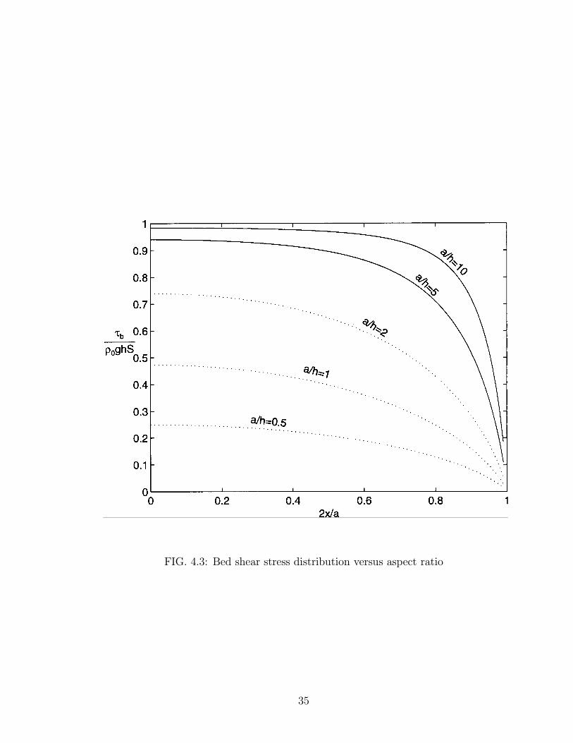
FIG. 4.3: Bed shear stress distribution versus aspect ratio
35
in which φc is deÞned as the side-wall correction factor for the centerline shear stress.
The corresponding shear velocity is obviously that
u∗ =pφcghS =
sgaS
πsin−1
µtanh
πh
a
¶(4.16)
According to Yang and Lim (1997), when the aspect ratio a/h > 2, the effect
of secondary currents on the channel centerline may be neglected. This implies that
(4.15) and (4.16) may be valid when a/h > 2. To be safe, say a/h > 2.5 in this
dissertation. (4.15) and (4.16) will be examined using Wang and Qians experimental
data where a/h = 3− 3.75 and Mustes data where a/h = 7.
4.4 Average bed shear stress and average bed shear
velocity
Although the above mapping model may not be valid for very narrow channels
where secondary currents are strong, the average bed shear stress is still based on
it. The result will be calibrated by introducing a secondary ßow correction factor.
Theoretically, the integration of (4.14) can give the average bed shear stress. However,
this is very complicated.
Consider the right half of the cross-section, shown in FIG. 4.1(a). The delimitation
CH in the z−plane corresponds to C 0H 0 in the w−plane, which is ξ = const. Since(x, y) = (a
2, 0) in the z−plane is a point in the delimitation CH, substituting this
point into (4.4) gives ξ = const = aπ, so the equation of the curve CH in the z−plane
from (4.4) is
sinπx
acosh
πy
a= 1
i.e.
πy
a= cosh−1
1
sinπx
a
= ln
1
sinπx
a
+
vuut 1
sin2πx
a
− 1
36
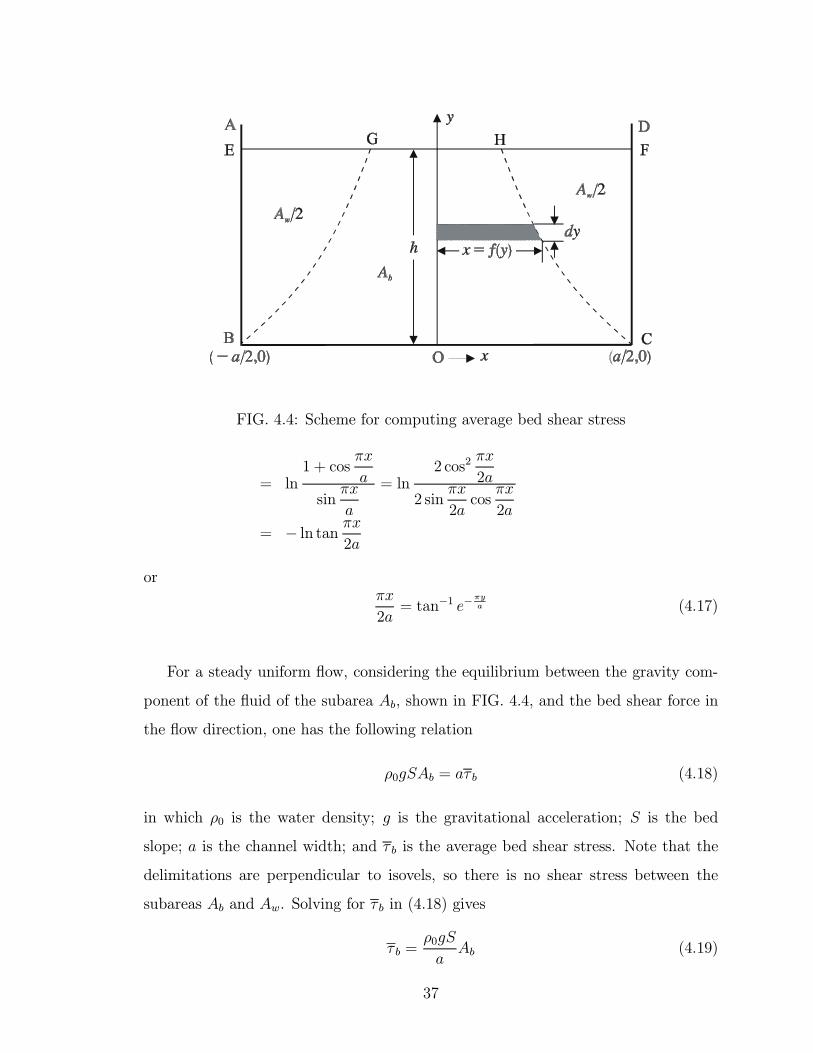
FIG. 4.4: Scheme for computing average bed shear stress
= ln1 + cos
πx
a
sinπx
a
= ln2 cos2
πx
2a
2 sinπx
2acos
πx
2a
= − ln tan πx2a
orπx
2a= tan−1 e−
πya (4.17)
For a steady uniform ßow, considering the equilibrium between the gravity com-
ponent of the ßuid of the subarea Ab, shown in FIG. 4.4, and the bed shear force in
the ßow direction, one has the following relation
ρ0gSAb = aτ b (4.18)
in which ρ0 is the water density; g is the gravitational acceleration; S is the bed
slope; a is the channel width; and τ b is the average bed shear stress. Note that the
delimitations are perpendicular to isovels, so there is no shear stress between the
subareas Ab and Aw. Solving for τ b in (4.18) gives
τ b =ρ0gS
aAb (4.19)
37
Referring to FIG. 4.4 and considering (4.17), one gets the subarea Ab as
Ab = 2
Z h
0
xdy =4a
π
Z h
0
tan−1 e−πya dy
The integration of the above equation by parts yields
Ab =4ah
πtan−1 e−
ayπ + 4
Z h
0
ye−πya
1 + e−2πyα
dy (4.20)
Numerical experiments show that the Þrst term on the right-hand side is the leading
term. The second term is only a small fraction of the Þrst one. Therefore, one may
approximate the second one asZ h
0
ye−πya
1 + e−2πyα
dy ≈Z λh
0
ye−πya dy =
³aπ
´2 ·1−
µ1 +
λπh
a
¶e−
λπha
¸(4.21)
Since the integrand has been enlarged, the correction factor λ in the upper limit
must be in 0 < λ < 1. This can be considered a secondary ßow correction factor.
Physically, not all the potential energy in the subarea Ab is dissipated by the bed
shear stress. A small fraction of potential energy is used to maintain the secondary
ßows. Therefore, λ must be less than unit. Now the subarea Ab may be interpreted
as the effective ßow area where the potential energy is dissipated by the bed shear
stress. Obviously, the subarea Ab under study now is less than the area in FIG. 4.4.
For convenience, the effective subarea is still denoted by Ab.
Substituting (4.21) into (4.20) gives the effective subarea Ab corresponding to the
bed shear stress as
Ab =4ah
πtan−1 e−
πya + 4
³aπ
´2 ·1−
µ1 +
λπh
a
¶e−
λπha
¸Furthermore, substituting this equation into (4.19) gives
τ b =ρ0gS
a
½4ah
πtan−1 e−
πya + 4
³aπ
´2 ·1−
µ1 +
λπh
a
¶e−
λπha
¸¾or
φm ≡ τ bρ0ghS
=4
πtan−1 e−
πya +
4a
π2h
·1−
µ1 +
λπh
a
¶e−
λπha
¸(4.22)
in which φm is deÞned as the side-wall correction factor for average bed shear stress.
The secondary correction factor λ is calibrated as 0.6691 using extensive experimental
38
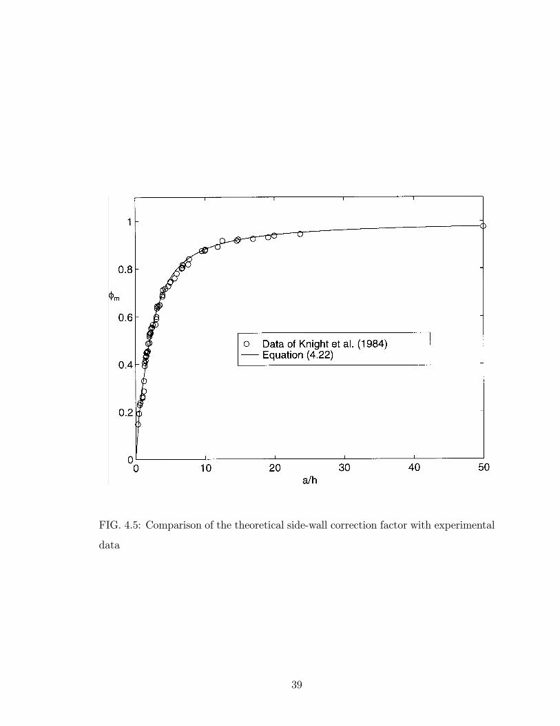
FIG. 4.5: Comparison of the theoretical side-wall correction factor with experimental
data
39
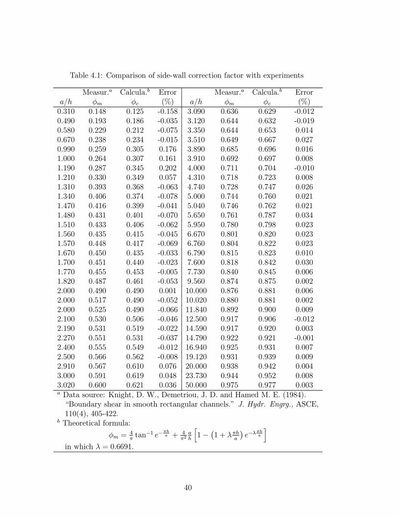
Table 4.1: Comparison of side-wall correction factor with experiments
Measur.a Calcula.b Error Measur.a Calcula.b Errora/h φm φc (%) a/h φm φc (%)0.310 0.148 0.125 -0.158 3.090 0.636 0.629 -0.0120.490 0.193 0.186 -0.035 3.120 0.644 0.632 -0.0190.580 0.229 0.212 -0.075 3.350 0.644 0.653 0.0140.670 0.238 0.234 -0.015 3.510 0.649 0.667 0.0270.990 0.259 0.305 0.176 3.890 0.685 0.696 0.0161.000 0.264 0.307 0.161 3.910 0.692 0.697 0.0081.190 0.287 0.345 0.202 4.000 0.711 0.704 -0.0101.210 0.330 0.349 0.057 4.310 0.718 0.723 0.0081.310 0.393 0.368 -0.063 4.740 0.728 0.747 0.0261.340 0.406 0.374 -0.078 5.000 0.744 0.760 0.0211.470 0.416 0.399 -0.041 5.040 0.746 0.762 0.0211.480 0.431 0.401 -0.070 5.650 0.761 0.787 0.0341.510 0.433 0.406 -0.062 5.950 0.780 0.798 0.0231.560 0.435 0.415 -0.045 6.670 0.801 0.820 0.0231.570 0.448 0.417 -0.069 6.760 0.804 0.822 0.0231.670 0.450 0.435 -0.033 6.790 0.815 0.823 0.0101.700 0.451 0.440 -0.023 7.600 0.818 0.842 0.0301.770 0.455 0.453 -0.005 7.730 0.840 0.845 0.0061.820 0.487 0.461 -0.053 9.560 0.874 0.875 0.0022.000 0.490 0.490 0.001 10.000 0.876 0.881 0.0062.000 0.517 0.490 -0.052 10.020 0.880 0.881 0.0022.000 0.525 0.490 -0.066 11.840 0.892 0.900 0.0092.100 0.530 0.506 -0.046 12.500 0.917 0.906 -0.0122.190 0.531 0.519 -0.022 14.590 0.917 0.920 0.0032.270 0.551 0.531 -0.037 14.790 0.922 0.921 -0.0012.400 0.555 0.549 -0.012 16.940 0.925 0.931 0.0072.500 0.566 0.562 -0.008 19.120 0.931 0.939 0.0092.910 0.567 0.610 0.076 20.000 0.938 0.942 0.0043.000 0.591 0.619 0.048 23.730 0.944 0.952 0.0083.020 0.600 0.621 0.036 50.000 0.975 0.977 0.003a Data source: Knight, D. W., Demetriou, J. D. and Hamed M. E. (1984).Boundary shear in smooth rectangular channels. J. Hydr. Engrg., ASCE,110(4), 405-422.
b Theoretical formula:
φm =4πtan−1 e−
πha + 4
π2ah
h1− ¡1 + λπh
a
¢e−λ
πha
iin which λ = 0.6691.
40
data (Knight et al., 1984). A comparison of (4.22) with experimental data is shown
in Table 4.1 and FIG. 4.5, where the correlation coefficient is 0.9961 and the average
relative error is 3.7%.
With the side-wall correction factor φm, the average bed shear velocity u∗ can be
calculated by the following:
u∗ =
rτ bρ0=pφmghS (4.23)
The above equation is derived from the model where the maximum velocity always
occurs at the water surface, but the parameter λ, determined experimentally, consid-
ers the effect of secondary ßows. Therefore, it is valid even if the maximum velocity
occurs below the water surface.
Empirically, (4.23) can be approximated as the centerline shear velocity when
a/h ≤ 2.5. This will be seen later from Colemans experimental data in Table 5.3,
where the aspect ratio a/h is about 2.
By the way, the side-wall shear stress distribution and its average shear stress
can also be calculated in a similar way. They are, however, neglected because of
irrelevance to this study.
4.5 Summary
In this chapter, the channel centerline shear velocity equation (4.16) is derived
based on the shear stress distribution along the bed. It may be valid for a/h > 2.5.
The average bed shear velocity, which is calculated from (4.22) and (4.23), may be
as a good approximation of the channel centerline shear velocity in narrow channels.
A secondary ßow correction factor is considered in the average bed shear velocity.
41
Chapter 5
TEST OF THE MODIFIED
LOG-WAKE LAW IN CLEAR
WATER
5.1 Introduction
The purposes of this chapter are to examine that: (1) is the structure of the
modiÞed log-wake law reasonable? (2) if the structure of the modiÞed log-wake law is
correct, how do the model parameters κ0, Ω0 and λ0 vary with the Reynolds number
u∗h/ν or the aspect ratio a/h? and (3) if the modiÞed log-wake law is correct, does
the corresponding eddy viscosity model agree with experimental data?
Since pipe ßows are simpler than open-channel ßows, the maximum velocity u1max
at a pipe axis and the shear velocity u∗ in a pipe can be exactly measured or estimated,
this test starts with the examination of the modiÞed log-wake law in pipes in Section
5.2. Narrow channel ßows are then tested in Section 5.3. Wide channel experiments
are tested in Sections 5.4 and 5.5. Note that a wide channel ßow is different from
that in a narrow channel since their derivative boundary conditions are not the same.
This can be easily seen from (2.12) and (2.13) in Chapter 2. Finally, Section 5.6
summaries the results of this chapter.
42
5.2 Test of the modiÞed log-wake law in pipes
5.2.1 ModiÞed log-wake law in pipes
Applying the boundary condition (2.13) to (3.30), or λ0 = 0 to (3.31), one gets
the modiÞed log-wake law in pipes as
u1max − u1u∗
= − 1κ0ln ξ + Ω0 cos
2 πξ
2− 1− ξ
κ0(5.1)
in which ξ = x3/R and R is the radius of the pipe.
5.2.2 Data selection
Since the classical experiments by Nikuradse (1932), many pipe experiments
have been reported, a systematic review of these experiments can be found in Za-
garolas (1996) dissertation. The latest accurate superpipe measurements by Za-
garola (1996) at the Gas Dynamics Lab in Princeton University will be used in this
study. Zagarola performed measurements of the mean velocity proÞles and static
pressure gradients at 26 different Reynolds numbers between 3.1×10⁴ and 3.5×10⁷.The complete description of the experimental details and experimental data can be
found in his dissertation (Zagarola, 1996) or a Web site in Princeton University:
http://www.princeton.edu/gasdyn/index.htmp. In this section, only the mean ve-
locity proÞle data are used to examine the modiÞed log-wake law. By the way, the
study of a power-wake law in pipes can be found in Appendix A. However, the power-
wake law is not emphasized in this dissertation.
In Zagarolas experimental data, the maximum velocity u1max, shear velocity u∗,
and sample points (ξi, ui) are given. Hence, only the von Karman constant κ0 and
the wake strength coefficient Ω0 are Þtting parameters.
5.2.3 Methods for determining κ0 and Ω0
Two methods can be used to determine κ0 and Ω0, one is the asymptotic method,
the other is the least-squares method.
43
Asymptotic method (Graphical method)
For a quick estimation, let ξ << 1, (5.1) reduces to the classical log law, i.e.
u1max − u1u∗
= − 1κ0ln ξ + Ω0 − 1
κ0(5.2)
Then the von Karman constant κ0 and the wake strength coefficient Ω0 can be de-
termined from the slope and intercept at ξ = 1 of a semilog plot of (u1max − u1) /u∗versus ξ. This method is similar to that suggested by Coles (1956) and Coleman
(1986) in the log-wake law. It is illustrated in FIG. 5.4 (p.51). The asymptotic
method is only illustrated herein and not used in this study.
Least-squares method
To accurately estimate κ0 and Ω0, the least-squares method should be used. The
least-squares approximation can be represented by
S =nXi
·u1max − u1i
u∗+1
κ0(ln ξi + 1− ξi)−Ω0 cos2 πξi
2
¸2=⇒ minimum (5.3)
in which S is the sum of the squares of the residuals; n is the number of sample points
(ξi, u1i); and u1max and u∗ are given. Then the model parameters κ0 and Ω0 can be
found by solving the following equations:
∂S
∂κ0= 0 and
∂S
∂Ω0= 0 (5.4)
That is,nXi
·u1max − u1i
u∗+1
κ0(ln ξi + 1− ξi)−Ω0 cos2 πξi
2
¸(ln ξi + 1− ξi) = 0 (5.5)
andnXi
·u1max − u1i
u∗+1
κ0(ln ξi + 1− ξi)− Ω0 cos2 πξi
2
¸cos2
πξi2= 0 (5.6)
The above two equations can be further written as
1
κ0
nXi
(ln ξi + 1− ξi)2 − Ω0nXi
(ln ξi + 1− ξi) cos2 πξi2
= −nXi
u1max − u1iu∗
(ln ξi + 1− ξi) (5.7)
44
and
1
κ0
nXi
(ln ξi + 1− ξi) cos2 πξi2− Ω0
nXi
cos4πξi2
= −nXi
u1max − u1iu∗
cos2πξi2
(5.8)
(5.7) and (5.8) are linear equations with respect to 1/κ0 and Ω0. A MatLab program
has been written to handle this solving process (Appendix B).
5.2.4 Test of the structure of the modiÞed log-wake law
Theoretically, the modiÞed log-wake law is valid in the outer region (overlap +
wake layer + boundary effect layer). The lower limit of the overlap is usually taken
as y+ = 70. Therefore, the modiÞed log-wake law is valid in y+ ≥ 70 and ξ ≤ 1. FIG.5.1 is a test of the structure of the modiÞed log-wake law. To emphasize the velocity
proÞle near the bed, a semilog plot is shown in FIG. 5.1a, where the modiÞed log-
wake law, the asymptotic log law and the asymptotic parabolic law are compared with
Zagarolas (1996) experimental data. The same things are plotted in a rectangular
coordinate system in FIG. 5.1b to emphasize the velocity proÞle near the axis. It
can be seen that the modiÞed log-wake law agrees fairly well with experimental data.
The correlation coefficient r = 0.9999, shown in FIG. 5.1b. Besides, the asymptotic
log law can be considered valid until about ξ = 0.1; and the asymptotic parabolic law
can be considered valid above ξ = 0.6. All other proÞles are very similar to those in
FIG. 5.1. No doubt, the structure of the modiÞed log-wake law is reasonable.
5.2.5 Test of κ0 and Ω0 with Reynolds number
The structure of the modiÞed log-wake law has been checked to be correct. Are
the model parameters κ0 and Ω0 universal or Reynolds number dependable constants?
FIG. 5.2 is a test of κ0 and Ω0 with Reynolds number. It shows that an excellent
agreement is obtained for each run. The individual values of κ0 and Ω0 are tabulated
in Table 5.1, where κ0 varies between 0.38 and 0.41 and can be approximated by
κ0 = 0.3527 + 0.0049 lnRe∗ (5.9)
45
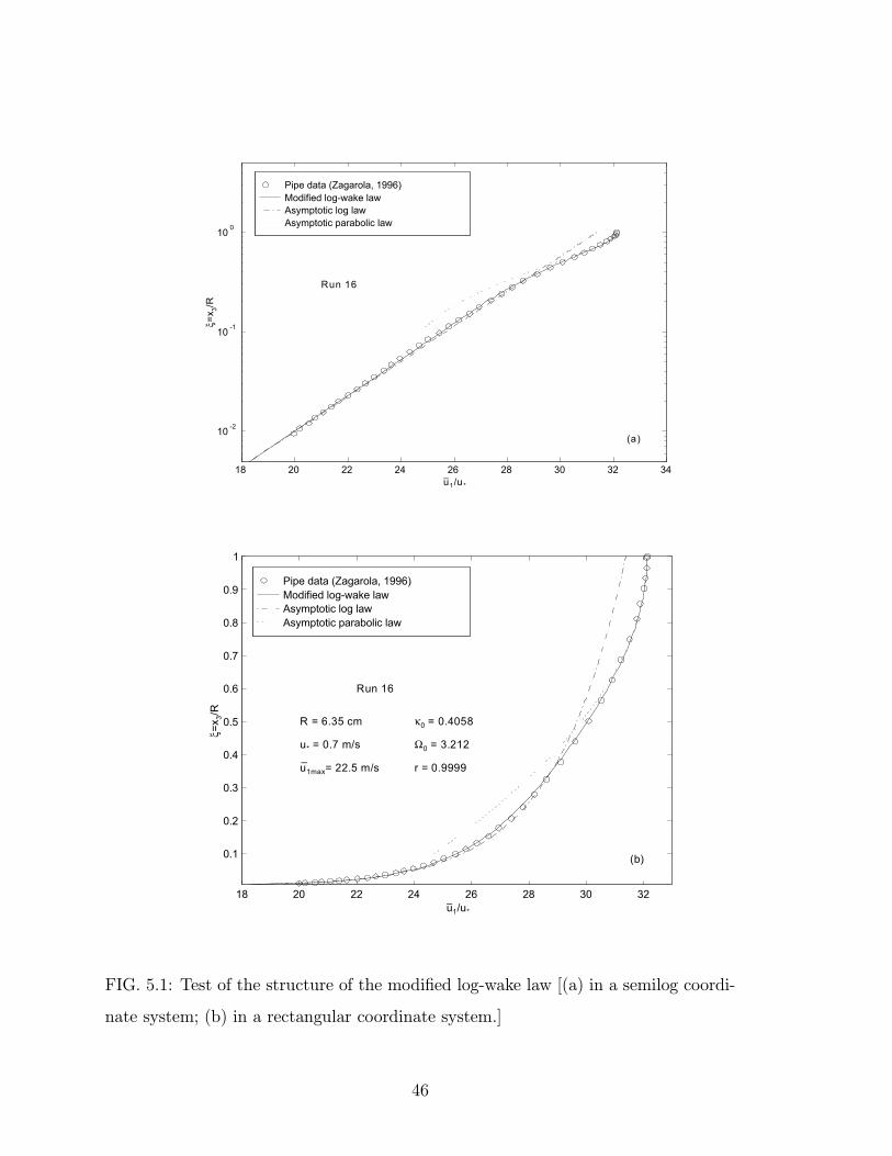
Pipe data (Zagarola, 1996)Modified log-wake law Asymptotic log law Asymptotic parabolic law
18 20 22 24 26 28 30 32 34
10 -2
10 -1
10 0
Run 16
ξ=x 3/
R
u−1/u*
(a)
Pipe data (Zagarola, 1996)Modified log-wake law Asymptotic log law Asymptotic parabolic law
18 20 22 24 26 28 30 32
0.1
0.2
0.3
0.4
0.5
0.6
0.7
0.8
0.9
1
ξ=x 3
/R
u−1/u*
Run 16
R = 6.35 cm
u* = 0.7 m/s
u1max= 22.5 m/s
κ0 = 0.4058
Ω0 = 3.212
r = 0.9999
(b)
FIG. 5.1: Test of the structure of the modiÞed log-wake law [(a) in a semilog coordi-
nate system; (b) in a rectangular coordinate system.]
46
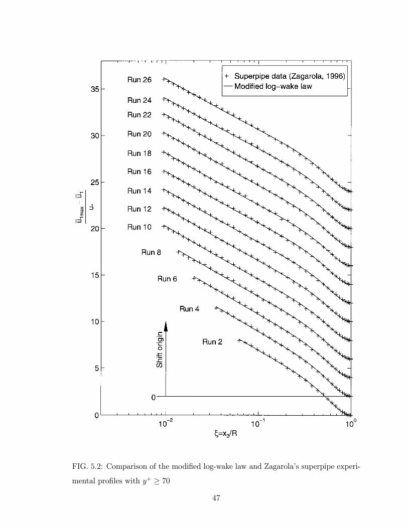
FIG. 5.2: Comparison of the modiÞed log-wake law and Zagarolas superpipe experi-
mental proÞles with y+ ≥ 7047
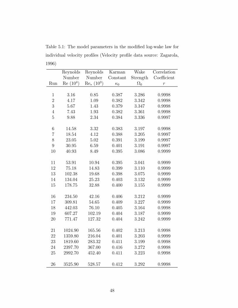
Table 5.1: The model parameters in the modiÞed log-wake law for
individual velocity proÞles (Velocity proÞle data source: Zagarola,
1996)
Reynolds Reynolds Karman Wake CorrelationNumber Number Constant Strength Coefficient
Run Re (104) Re∗ (103) κ0 Ω0 r
1 3.16 0.85 0.387 3.286 0.99982 4.17 1.09 0.382 3.342 0.99983 5.67 1.43 0.379 3.347 0.99984 7.43 1.93 0.382 3.361 0.99985 9.88 2.34 0.384 3.336 0.9997
6 14.58 3.32 0.383 3.197 0.99987 18.54 4.12 0.388 3.205 0.99978 23.05 5.02 0.391 3.199 0.99979 30.95 6.59 0.401 3.191 0.999710 40.93 8.49 0.395 3.086 0.9999
11 53.91 10.94 0.395 3.041 0.999912 75.18 14.83 0.399 3.110 0.999913 102.38 19.68 0.398 3.075 0.999914 134.04 25.23 0.403 3.132 0.999915 178.75 32.88 0.400 3.155 0.9999
16 234.50 42.16 0.406 3.212 0.999917 309.81 54.65 0.409 3.227 0.999918 442.03 76.10 0.405 3.164 0.999819 607.27 102.19 0.404 3.187 0.999920 771.47 127.32 0.404 3.242 0.9999
21 1024.90 165.56 0.402 3.213 0.999822 1359.80 216.04 0.401 3.203 0.999923 1819.60 283.32 0.411 3.199 0.999824 2397.70 367.00 0.416 3.272 0.999825 2992.70 452.40 0.411 3.223 0.9998
26 3525.90 528.57 0.412 3.292 0.9998
48
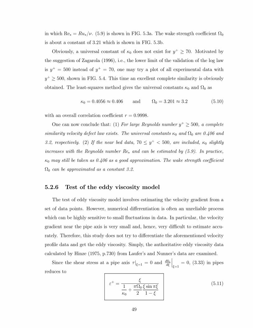
in which Re∗ = Ru∗/ν. (5.9) is shown in FIG. 5.3a. The wake strength coefficient Ω0
is about a constant of 3.21 which is shown in FIG. 5.3b.
Obviously, a universal constant of κ0 does not exist for y+ ≥ 70. Motivated by
the suggestion of Zagarola (1996), i.e., the lower limit of the validation of the log law
is y+ = 500 instead of y+ = 70, one may try a plot of all experimental data with
y+ ≥ 500, shown in FIG. 5.4. This time an excellent complete similarity is obviouslyobtained. The least-squares method gives the universal constants κ0 and Ω0 as
κ0 = 0.4056 ≈ 0.406 and Ω0 = 3.201 ≈ 3.2 (5.10)
with an overall correlation coefficient r = 0.9998.
One can now conclude that: (1) For large Reynolds number y+ ≥ 500, a completesimilarity velocity defect law exists. The universal constants κ0 and Ω0 are 0.406 and
3.2, respectively. (2) If the near bed data, 70 ≤ y+ < 500, are included, κ0 slightly
increases with the Reynolds number Re∗ and can be estimated by (5.9). In practice,
κ0 may still be taken as 0.406 as a good approximation. The wake strength coefficient
Ω0 can be approximated as a constant 3.2.
5.2.6 Test of the eddy viscosity model
The test of eddy viscosity model involves estimating the velocity gradient from a
set of data points. However, numerical differentiation is often an unreliable process
which can be highly sensitive to small ßuctuations in data. In particular, the velocity
gradient near the pipe axis is very small and, hence, very difficult to estimate accu-
rately. Therefore, this study does not try to differentiate the aforementioned velocity
proÞle data and get the eddy viscosity. Simply, the authoritative eddy viscosity data
calculated by Hinze (1975, p.730) from Laufers and Nunners data are examined.
Since the shear stress at a pipe axis τ |ξ=1 = 0 and du1dξ
¯ξ=1
= 0, (3.33) in pipes
reduces to
ε+ =ξ
1
κ0+πΩ02
ξ sin πξ
1− ξ(5.11)
49
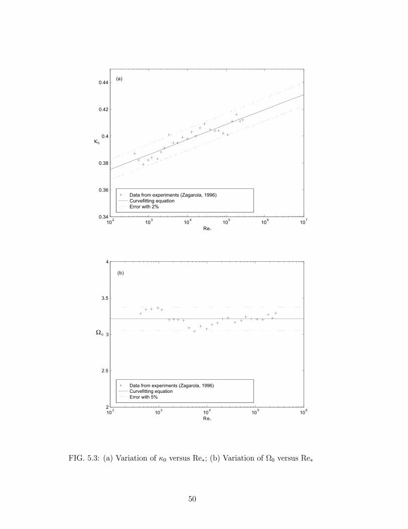
Data from experiments (Zagarola, 1996)Curvefitting equation Error with 2%
102 103 104 105 106 1070.34
0.36
0.38
0.4
0.42
0.44
Re*
κ0
(a)
Data from experiments (Zagarola, 1996)Curvefitting equation Error with 5%
10 2 103 10 4 10 5 1062
2.5
3
3.5
4
Re*
Ω 0
(b)
FIG. 5.3: (a) Variation of κ0 versus Re∗; (b) Variation of Ω0 versus Re∗
50
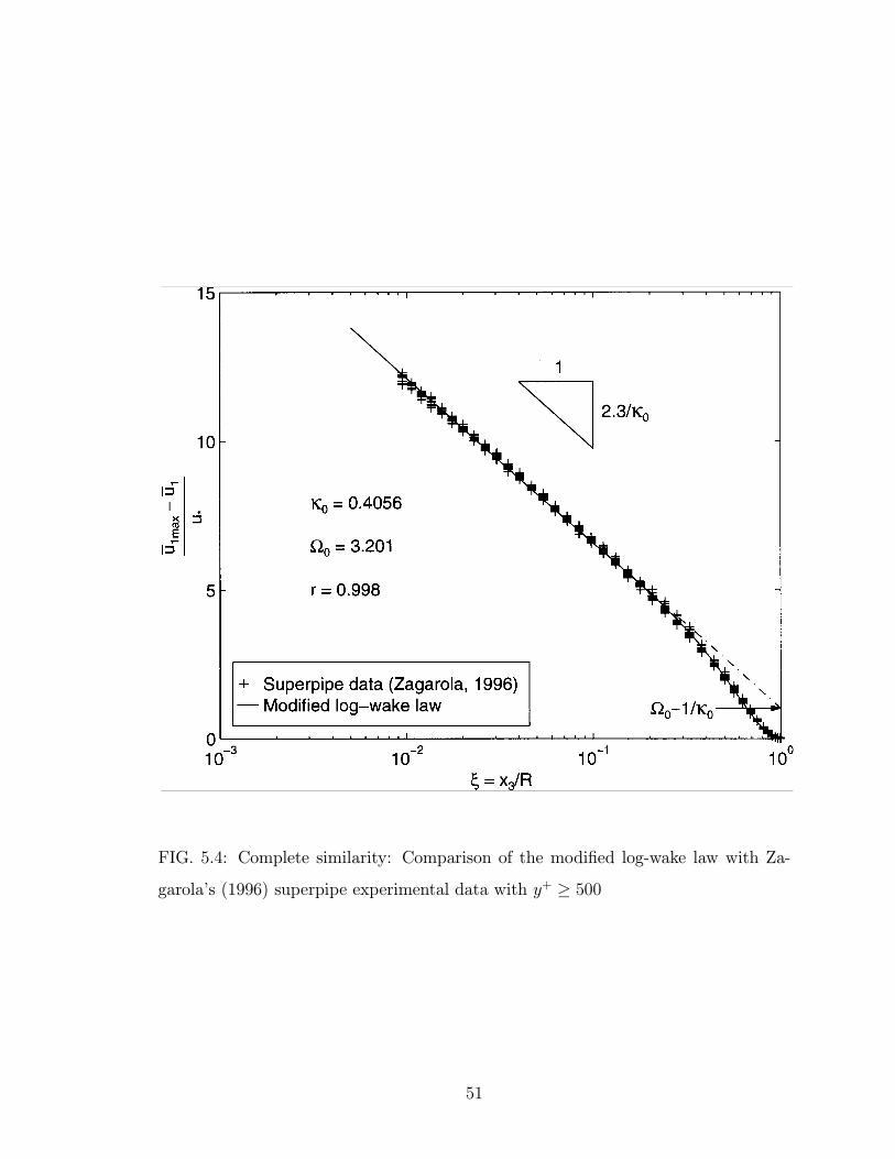
FIG. 5.4: Complete similarity: Comparison of the modiÞed log-wake law with Za-
garolas (1996) superpipe experimental data with y+ ≥ 500
51
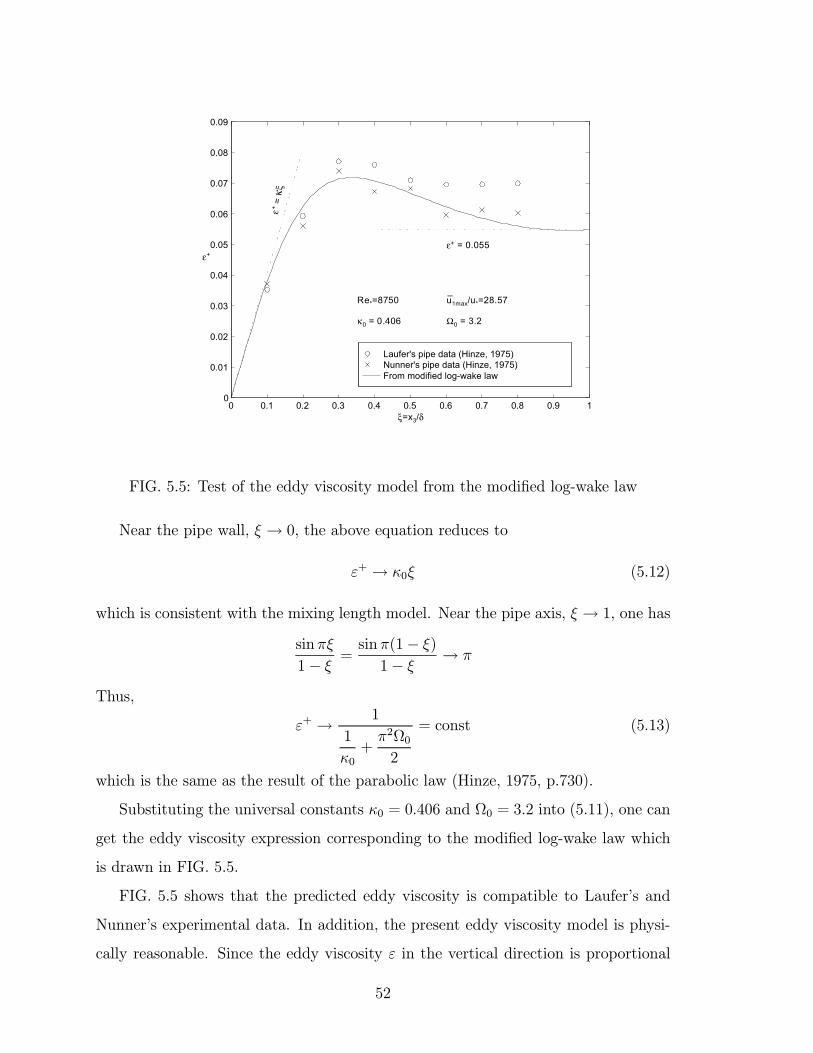
Laufer's pipe data (Hinze, 1975)Nunner's pipe data (Hinze, 1975)From modified log-wake law
0 0.1 0.2 0.3 0.4 0.5 0.6 0.7 0.8 0.9 10
0.01
0.02
0.03
0.04
0.05
0.06
0.07
0.08
0.09
ξ=x3/δ
ε+
u1max/u*=28.57Re*=8750
κ0 = 0.406 Ω0 = 3.2
ε+ = 0.055
ε+ =
κξ
FIG. 5.5: Test of the eddy viscosity model from the modiÞed log-wake law
Near the pipe wall, ξ → 0, the above equation reduces to
ε+ → κ0ξ (5.12)
which is consistent with the mixing length model. Near the pipe axis, ξ → 1, one has
sin πξ
1− ξ =sin π(1− ξ)1− ξ → π
Thus,
ε+ → 1
1
κ0+π2Ω02
= const (5.13)
which is the same as the result of the parabolic law (Hinze, 1975, p.730).
Substituting the universal constants κ0 = 0.406 and Ω0 = 3.2 into (5.11), one can
get the eddy viscosity expression corresponding to the modiÞed log-wake law which
is drawn in FIG. 5.5.
FIG. 5.5 shows that the predicted eddy viscosity is compatible to Laufers and
Nunners experimental data. In addition, the present eddy viscosity model is physi-
cally reasonable. Since the eddy viscosity ε in the vertical direction is proportional
52
to u03, the plot of the viscosity model is very similar to that of the measurements of
the turbulence intensity in the x3−direction (Hinze, 1975, p.725).
5.3 Test of the modiÞed log-wake law in narrow
open-channels
As stated earlier, the boundary layer thickness δ is the distance from the bed to
the maximum velocity u1max in narrow channels. The derivative boundary condition,
as it in pipes, is expressed by (2.13). Thus, the modiÞed log-wake law in narrow
channels is the same as that in pipes, i.e., (5.1), here ξ = x3/δ in narrow channels.
5.3.1 Data selection
Although many experiments in narrow ßumes are reported (Hu and Hui, 1995;
Sarma, Lakshminarayana and Rao, 1983), the original data can be found only in a few
papers. Three data sources are used here: Wang and Qian (1989), Coleman (1986),
and Kironoto (1993).
In Wang and Qians (1989) data, the experiments were run in a smooth ßume
(both side-walls and bed) with a bed slope S = 0.01, the aspect ratios are 3, 3.33
and 3.75. Therefore, the centerline shear velocity can be estimated from (4.16). The
detailed information can be found in Appendix C.
Colemans (1986) experiments are very similar to Wang and Qians (1989), except
that the bed slope S = 0.002 and the aspect ratios are about 2. Therefore, the
centerline shear velocity may be estimated from (4.23). Some information about
Colemans experiments is shown in Appendix D.
In both Wang and Qians (1989) and Colemans (1986) experiments, given the
shear velocity u∗, the Þtting parameters include δ, u1max, κ0, and Ω0. If κ0 is Þtted
as about 0.406 in these two data sets, it may be proved that the proposed equations
for determining the shear velocity u∗ in Chapter 4 are reasonable.
Kironoto (1993) did experiments over a rough bed (ks = 23 mm) ßume with the
53
aspect ratio a/h ≈ 2. So, the centerline shear velocity u∗ can be estimated from
neither (4.16) nor (4.23). In this case, one assumes that κ0 = 0.406, then the Þtting
parameters are u∗, δ, u1max, and Ω0. Some information about Kironotos (1993)
experiments can be found in Appendix E.
5.3.2 Method for determining δ and u1max
For a narrow channel where the maximum velocity occurs below the water surface,
one can assume that the velocity proÞle near the boundary layer margin (approxi-
mately ξ ≥ 0.6 from the pipe results) obeys the parabolic law, Þtting the experimentaldata (x3i, u1i) near the boundary layer margin as a quadratic equation can give the
maximum velocity u1max and its corresponding boundary layer thickness δ.
SpeciÞcally, let the velocity proÞle near the boundary layer margin has the follow-
ing functional form:
u1 = a1x23 + a2x3 + a3 (5.14)
in which a1, a2, and a3 are curve-Þtting constants. Using the experimental data
(x3i, u1i) near the boundary layer margin with the least-squares method, three con-
stants a1, a2, and a3 can be determined. Then, the boundary layer thickness δ and
the maximum velocity u1max can be easily estimated by setting the velocity gradient
du1/dx3 = 0, which gives
δ = − a22a1
(5.15)
u1max = a1δ2 + a2δ + a3 (5.16)
With δ, u1max and u∗ or κ0 available, the exact same procedure as that in pipes
is used for determining Ω0 and κ0 or u∗.
5.3.3 Test of the modiÞed log-wake law
Wang and Qians (1989) experiments
As stated earlier, the centerline shear velocities can be calculated from (4.16).
After determining the values of δ and u1max from (5.15) and (5.16), respectively, κ0
54
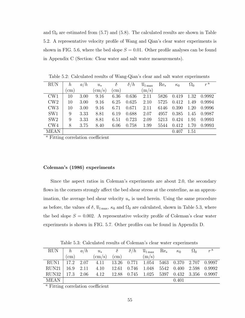
and Ω0 are estimated from (5.7) and (5.8). The calculated results are shown in Table
5.2. A representative velocity proÞle of Wang and Qians clear water experiments is
shown in FIG. 5.6, where the bed slope S = 0.01. Other proÞle analyses can be found
in Appendix C (Section: Clear water and salt water measurements).
Table 5.2: Calculated results of Wang-Qians clear and salt water experiments
RUN h a/h u∗ δ δ/h u1max Re∗ κ0 Ω0 r a
(cm) (cm/s) (cm) (m/s)CW1 10 3.00 9.16 6.36 0.636 2.11 5826 0.419 1.32 0.9992CW2 10 3.00 9.16 6.25 0.625 2.10 5725 0.412 1.49 0.9994CW3 10 3.00 9.16 6.71 0.671 2.11 6146 0.390 1.20 0.9996SW1 9 3.33 8.81 6.19 0.688 2.07 4957 0.385 1.45 0.9987SW2 9 3.33 8.81 6.51 0.723 2.09 5213 0.424 1.91 0.9993CW4 8 3.75 8.40 6.06 0.758 1.99 5544 0.412 1.70 0.9993MEAN 0.407 1.51a Fitting correlation coefficient
Colemans (1986) experiments
Since the aspect ratios in Colemans experiments are about 2.0, the secondary
ßows in the corners strongly affect the bed shear stress at the centerline, as an approx-
imation, the average bed shear velocity u∗ is used herein. Using the same procedure
as before, the values of δ, u1max, κ0 and Ω0 are calculated, shown in Table 5.3, where
the bed slope S = 0.002. A representative velocity proÞle of Colemans clear water
experiments is shown in FIG. 5.7. Other proÞles can be found in Appendix D.
Table 5.3: Calculated results of Colemans clear water experiments
RUN h a/h u∗ δ δ/h u1max Re∗ κ0 Ω0 r a
(cm) (cm/s) (cm) (m/s)RUN1 17.2 2.07 4.11 13.26 0.771 1.054 5463 0.370 2.707 0.9997RUN21 16.9 2.11 4.10 12.61 0.746 1.048 5542 0.400 2.598 0.9992RUN32 17.3 2.06 4.12 12.88 0.745 1.025 5397 0.432 3.356 0.9997MEAN 0.401a Fitting correlation coefficient
55
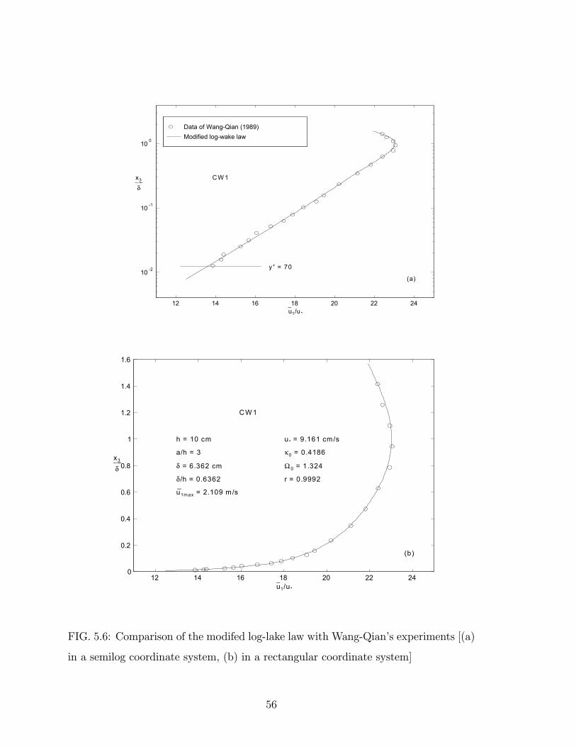
Data of Wang-Qian (1989)Modified log-wake law
12 14 16 18 20 22 24
10 -2
10 -1
10 0
u−1/u *
x3
δ___ CW 1
(a)
y+ = 70
12 14 16 18 20 22 240
0.2
0.4
0.6
0.8
1
1.2
1.4
1.6
u−1/u*
x3
δ___
CW 1
h = 10 cm
a/h = 3
δ = 6.362 cm
δ/h = 0.6362
u1max = 2.109 m/s
u* = 9.161 cm/s
κ0 = 0.4186
Ω 0 = 1.324
r = 0.9992
(b)
FIG. 5.6: Comparison of the modifed log-lake law with Wang-Qians experiments [(a)
in a semilog coordinate system, (b) in a rectangular coordinate system]
56
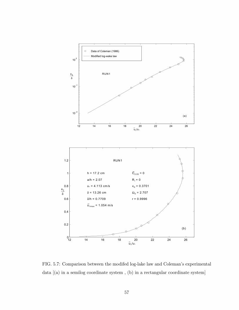
Data of Coleman (1986)
Modified log-wake law
12 14 16 18 20 22 24 26
10 -2
10 -1
10 0
u−1/u *
x3
δ___ RUN1
(a)
12 14 16 18 20 22 24 260
0.2
0.4
0.6
0.8
1
1.2
u−1/u*
x3
δ___
RUN1
h = 17.2 cm
a/h = 2.07
u* = 4.113 cm/s
δ = 13.26 cm
δ/h = 0.7709
u1max = 1.054 m/s
C0.05 = 0
Ri = 0
κ0 = 0.3701
Ω0 = 2.707
r = 0.9996
(b)
FIG. 5.7: Comparison between the modifed log-lake law and Colemans experimental
data [(a) in a semilog coordinate system , (b) in a rectangular coordinate system]
57
Data of Kironoto (1993)
Modified log-wake law
2 4 6 8 10 12 14
10 -2
10 -1
10 0
u−1/u*
x3
δ___ UGA5
(a)
2 4 6 8 10 12 140
0.2
0.4
0.6
0.8
1
1.2
u−1/u*
x3
δ___
UGA5 (ks=23 mm)
h = 28.5 cm
a/h = 2.11
δ = 21.81 cm
δ/h = 0.7653
u1max = 0.57 m/s
u* = 4.592 cm/s
κ0 = 0.406
Ω0 = 1.259
r = 0.9995
(b)
FIG. 5.8: Comparison between the modifed log-lake law and Kironotos narrow ßume
data [(a) in a semilog coordinate system, (b) in a rectangular coordinate system]
58
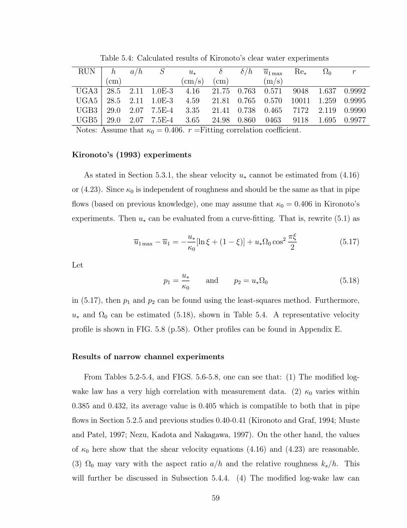
Table 5.4: Calculated results of Kironotos clear water experiments
RUN h a/h S u∗ δ δ/h u1max Re∗ Ω0 r(cm) (cm/s) (cm) (m/s)
UGA3 28.5 2.11 1.0E-3 4.16 21.75 0.763 0.571 9048 1.637 0.9992UGA5 28.5 2.11 1.0E-3 4.59 21.81 0.765 0.570 10011 1.259 0.9995UGB3 29.0 2.07 7.5E-4 3.35 21.41 0.738 0.465 7172 2.119 0.9990UGB5 29.0 2.07 7.5E-4 3.65 24.98 0.860 0463 9118 1.695 0.9977Notes: Assume that κ0 = 0.406. r =Fitting correlation coefficient.
Kironotos (1993) experiments
As stated in Section 5.3.1, the shear velocity u∗ cannot be estimated from (4.16)
or (4.23). Since κ0 is independent of roughness and should be the same as that in pipe
ßows (based on previous knowledge), one may assume that κ0 = 0.406 in Kironotos
experiments. Then u∗ can be evaluated from a curve-Þtting. That is, rewrite (5.1) as
u1max − u1 = −u∗κ0[ln ξ + (1− ξ)] + u∗Ω0 cos2 πξ
2(5.17)
Let
p1 =u∗κ0
and p2 = u∗Ω0 (5.18)
in (5.17), then p1 and p2 can be found using the least-squares method. Furthermore,
u∗ and Ω0 can be estimated (5.18), shown in Table 5.4. A representative velocity
proÞle is shown in FIG. 5.8 (p.58). Other proÞles can be found in Appendix E.
Results of narrow channel experiments
From Tables 5.2-5.4, and FIGS. 5.6-5.8, one can see that: (1) The modiÞed log-
wake law has a very high correlation with measurement data. (2) κ0 varies within
0.385 and 0.432, its average value is 0.405 which is compatible to both that in pipe
ßows in Section 5.2.5 and previous studies 0.40-0.41 (Kironoto and Graf, 1994; Muste
and Patel, 1997; Nezu, Kadota and Nakagawa, 1997). On the other hand, the values
of κ0 here show that the shear velocity equations (4.16) and (4.23) are reasonable.
(3) Ω0 may vary with the aspect ratio a/h and the relative roughness ks/h. This
will further be discussed in Subsection 5.4.4. (4) The modiÞed log-wake law can
59
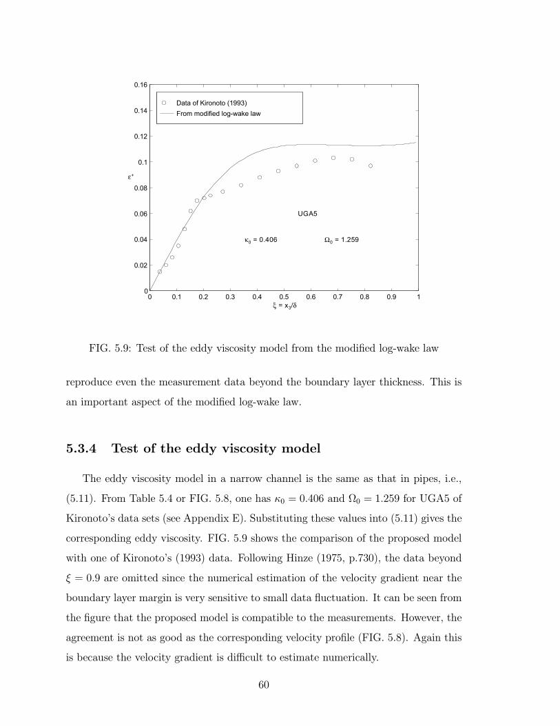
Data of Kironoto (1993) From modified log-wake law
0 0.1 0.2 0.3 0.4 0.5 0.6 0.7 0.8 0.9 10
0.02
0.04
0.06
0.08
0.1
0.12
0.14
0.16
UGA5
κ0 = 0.406 Ω0 = 1.259
ξ = x3/δ
ε+
FIG. 5.9: Test of the eddy viscosity model from the modiÞed log-wake law
reproduce even the measurement data beyond the boundary layer thickness. This is
an important aspect of the modiÞed log-wake law.
5.3.4 Test of the eddy viscosity model
The eddy viscosity model in a narrow channel is the same as that in pipes, i.e.,
(5.11). From Table 5.4 or FIG. 5.8, one has κ0 = 0.406 and Ω0 = 1.259 for UGA5 of
Kironotos data sets (see Appendix E). Substituting these values into (5.11) gives the
corresponding eddy viscosity. FIG. 5.9 shows the comparison of the proposed model
with one of Kironotos (1993) data. Following Hinze (1975, p.730), the data beyond
ξ = 0.9 are omitted since the numerical estimation of the velocity gradient near the
boundary layer margin is very sensitive to small data ßuctuation. It can be seen from
the Þgure that the proposed model is compatible to the measurements. However, the
agreement is not as good as the corresponding velocity proÞle (FIG. 5.8). Again this
is because the velocity gradient is difficult to estimate numerically.
60
5.4 Test of the modiÞed log-wake law in wide open-
channels
5.4.1 Data selection
In the test of the modiÞed log-wake law in wide channels, if one assumes κ0 =
0.406, there are still four Þtting parameters, u∗, Ω0, λ0 and u1max. More Þtting
parameters will reduce the reliability of the Þtting results. Therefore, this test will
only use the experimental data reported by Kironoto (1993), where the maximum
velocity u1max is measured. Only three parameters, u∗, Ω0, and λ0, need to be Þtted.
In addition, the channel side-walls are smooth and the bed is rough with ks = 4.8
mm. The aspect ratios a/h are between 5 and 7.
5.4.2 Method for determining u∗, Ω0, and λ0
The modiÞed log-wake law is described by (3.31) in wide open-channels, where
the water surface shear effect factor λ0 6= 0. Rewrite (5.23) as
u1max − u1 = −u∗κ0[ln ξ + (1− ξ)] + Ω0u∗ cos2 πξ
2
+λ0
µVwind − u1max
u∗
¶2u∗(1− ξ) (5.19)
Let
p1 =u∗κ0
, p2 = Ω0u∗ , p3 = λ0
µVwind − u1max
u∗
¶2u∗ (5.20)
then p1, p2 and p3 can be estimated by the least-squares method (linear regression).
A MatLab program to handle the above process is appended in Appendix B.
With p1, p2 and p3 available, one has
u∗ = κ0p1 , Ω0 = p2/u∗ , λ0 =p3u∗
µVwind − u1max
u∗
¶−2
5.4.3 Test of the modiÞed log-wake law
The calculated results of Kironotos (1993) data in a wide ßume are shown in
Table 5.5. A representative velocity proÞle, along with the modiÞed log-wake law,
61
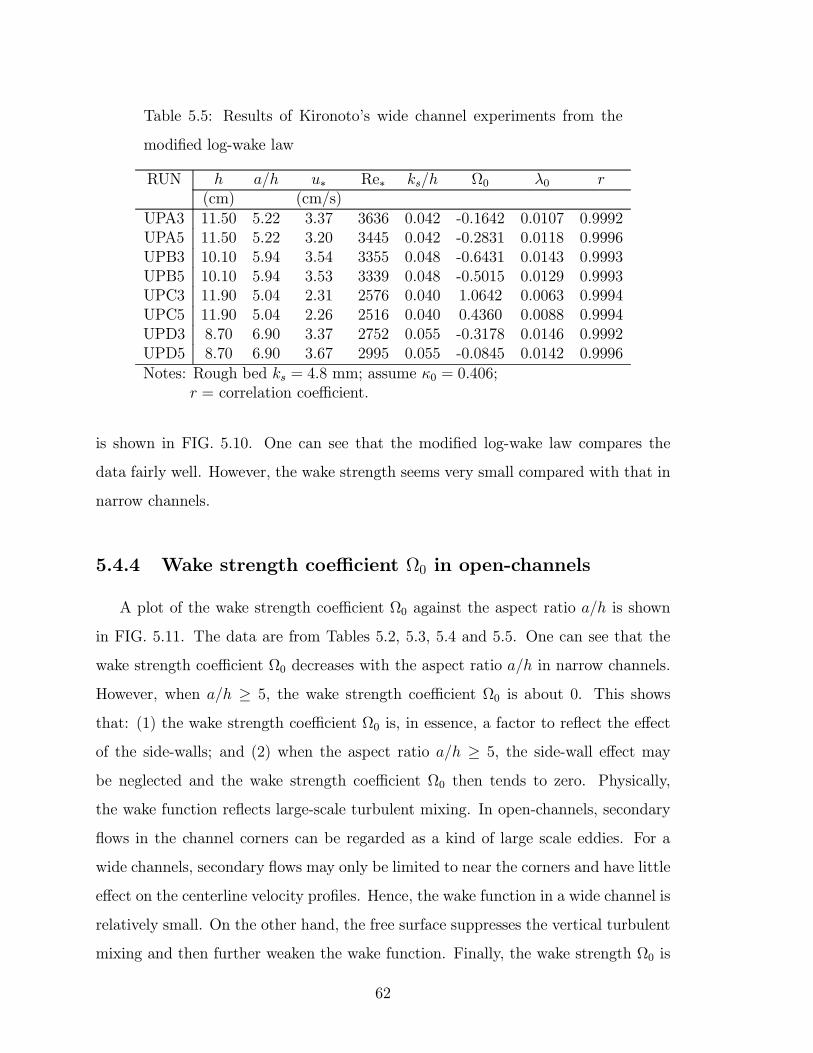
Table 5.5: Results of Kironotos wide channel experiments from the
modiÞed log-wake law
RUN h a/h u∗ Re∗ ks/h Ω0 λ0 r(cm) (cm/s)
UPA3 11.50 5.22 3.37 3636 0.042 -0.1642 0.0107 0.9992UPA5 11.50 5.22 3.20 3445 0.042 -0.2831 0.0118 0.9996UPB3 10.10 5.94 3.54 3355 0.048 -0.6431 0.0143 0.9993UPB5 10.10 5.94 3.53 3339 0.048 -0.5015 0.0129 0.9993UPC3 11.90 5.04 2.31 2576 0.040 1.0642 0.0063 0.9994UPC5 11.90 5.04 2.26 2516 0.040 0.4360 0.0088 0.9994UPD3 8.70 6.90 3.37 2752 0.055 -0.3178 0.0146 0.9992UPD5 8.70 6.90 3.67 2995 0.055 -0.0845 0.0142 0.9996Notes: Rough bed ks = 4.8 mm; assume κ0 = 0.406;
r = correlation coefficient.
is shown in FIG. 5.10. One can see that the modiÞed log-wake law compares the
data fairly well. However, the wake strength seems very small compared with that in
narrow channels.
5.4.4 Wake strength coefficient Ω0 in open-channels
A plot of the wake strength coefficient Ω0 against the aspect ratio a/h is shown
in FIG. 5.11. The data are from Tables 5.2, 5.3, 5.4 and 5.5. One can see that the
wake strength coefficient Ω0 decreases with the aspect ratio a/h in narrow channels.
However, when a/h ≥ 5, the wake strength coefficient Ω0 is about 0. This shows
that: (1) the wake strength coefficient Ω0 is, in essence, a factor to reßect the effect
of the side-walls; and (2) when the aspect ratio a/h ≥ 5, the side-wall effect may
be neglected and the wake strength coefficient Ω0 then tends to zero. Physically,
the wake function reßects large-scale turbulent mixing. In open-channels, secondary
ßows in the channel corners can be regarded as a kind of large scale eddies. For a
wide channels, secondary ßows may only be limited to near the corners and have little
effect on the centerline velocity proÞles. Hence, the wake function in a wide channel is
relatively small. On the other hand, the free surface suppresses the vertical turbulent
mixing and then further weaken the wake function. Finally, the wake strength Ω0 is
62
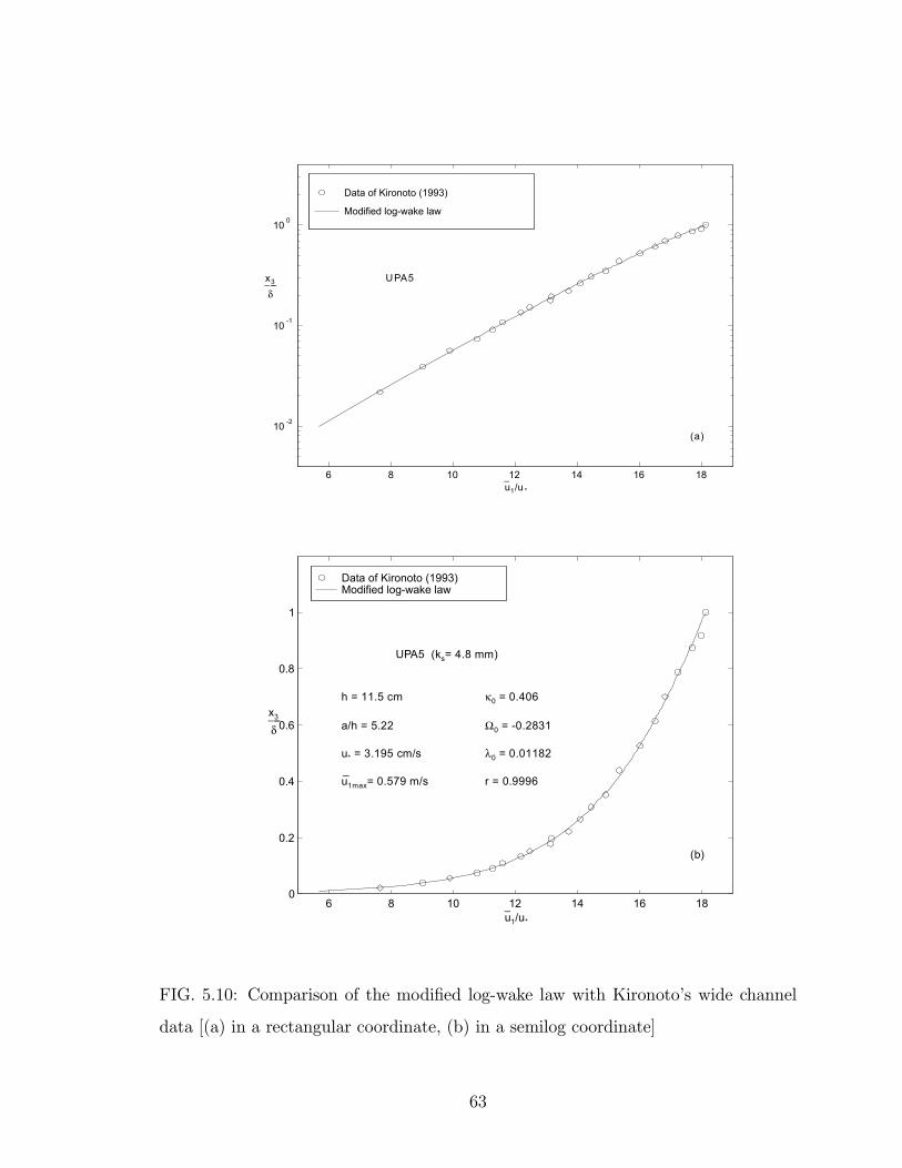
Data of Kironoto (1993)
Modified log-wake law
6 8 10 12 14 16 18
10 -2
10 -1
10 0
u−1/u *
x3
δ___ UPA5
(a)
Data of Kironoto (1993)Modified log-wake law
6 8 10 12 14 16 180
0.2
0.4
0.6
0.8
1
u−1/u*
x3
δ___
UPA5 (ks= 4.8 mm)
h = 11.5 cm
a/h = 5.22
u* = 3.195 cm/s
u1max= 0.579 m/s
κ0 = 0.406
Ω0 = -0.2831
λ0 = 0.01182
r = 0.9996
(b)
FIG. 5.10: Comparison of the modiÞed log-wake law with Kironotos wide channel
data [(a) in a rectangular coordinate, (b) in a semilog coordinate]
63
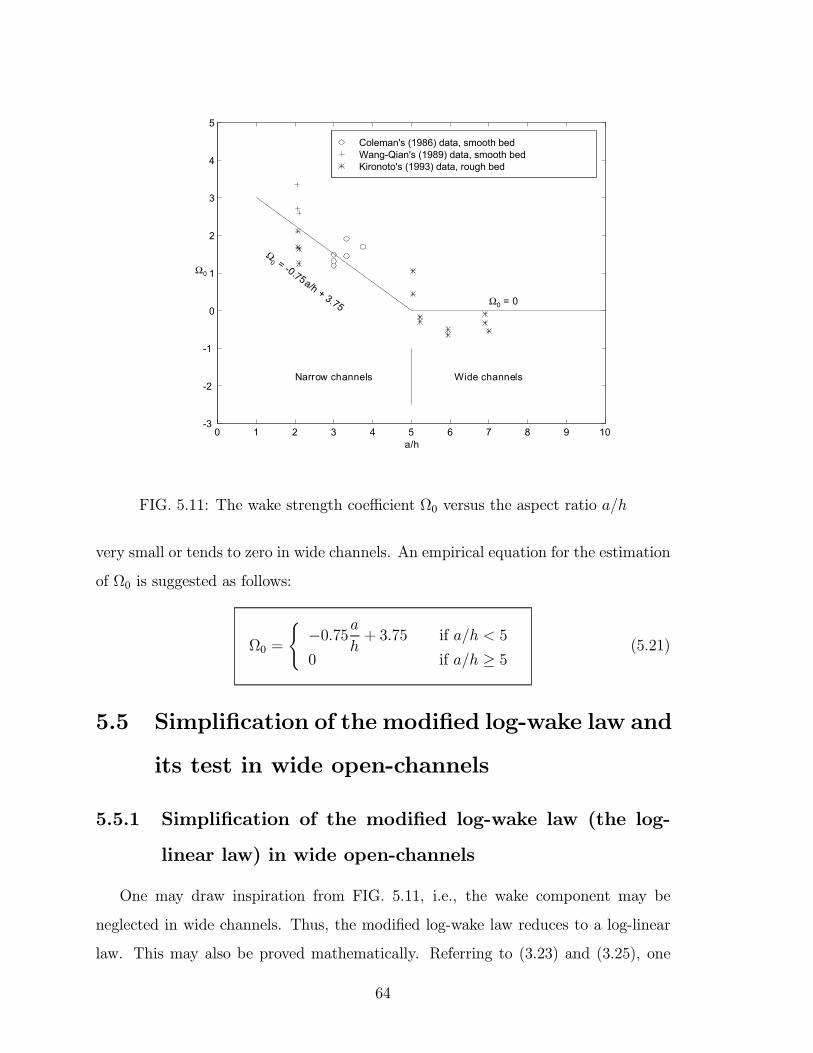
Coleman's (1986) data, smooth bed Wang-Qian's (1989) data, smooth bedKironoto's (1993) data, rough bed
0 1 2 3 4 5 6 7 8 9 10-3
-2
-1
0
1
2
3
4
5
Ω0 = -0.75a/h + 3.75 Ω0 = 0
Narrow channels Wide channels
a/h
Ω0
FIG. 5.11: The wake strength coefficient Ω0 versus the aspect ratio a/h
very small or tends to zero in wide channels. An empirical equation for the estimation
of Ω0 is suggested as follows:
Ω0 =
(−0.75a
h+ 3.75 if a/h < 5
0 if a/h ≥ 5(5.21)
5.5 SimpliÞcation of the modiÞed log-wake law and
its test in wide open-channels
5.5.1 SimpliÞcation of the modiÞed log-wake law (the log-
linear law) in wide open-channels
One may draw inspiration from FIG. 5.11, i.e., the wake component may be
neglected in wide channels. Thus, the modiÞed log-wake law reduces to a log-linear
law. This may also be proved mathematically. Referring to (3.23) and (3.25), one
64
can expand the modiÞed log-wake law at the water surface, i.e.
u1max − u1u∗
= − 1u∗
du1dξ
¯ξ=1
(1− ξ) +µ1
2κ0+ Ω0
¶(1− ξ)2 + · · · (5.22)
In pipes and narrow channels, du1dξ
¯ξ=1
= 0, the leading term is a second order
term³
12κ0+ Ω0
´(1 − ξ)2 near the water surface, which relates to the wake strength
coefficient Ω0. Therefore, the wake component is certainly important. In wide
channels, however, du1dξ
¯ξ=1
6= 0, the leading term is obviously a Þrst order term
− 1u∗
du1dξ
¯ξ=1(1 − ξ), which is irrelevant to the wake strength coefficient Ω0. As a
Þrst approximation, i.e., neglecting the second and higher order terms, one can see
that the wake strength coefficient Ω0 just has little effect on the ßow near the water
surface. That is, the wake component may be neglected in wide channels, i.e.,
u1max − u1u∗
= − 1κ0ln ξ −
"1
κ0− 1
u∗
du1dξ
¯ξ=1
#(1− ξ)
or
u1max − u1u∗
= − 1κ0ln ξ −
"1
κ0− λ0
µVwind − u1max
u∗
¶2#(1− ξ) (5.23)
in which λ0 is the water surface shear effect factor and will be determined experimen-
tally. The above equation is the simpliÞcation of the modiÞed log-wake law in wide
open-channels. For simplicity, it is referred to as the log-linear law. Note that this
log-linear law is different from (2.22) where it is only valid for sediment-laden ßows.
Let κ0 = 0.406, the Þtting parameters in the log-linear law are u1max, u∗, and λ0.
5.5.2 Data selection
Besides the data of Kironoto (1993) in Subsection 5.4.1, experiments by Muste
(1995), McQuivey (1971), and Guy, Simons and Richardson (1966) will also be used
in this section. Muste (1995) recorded 3 clear water experiments (Appendix F) in a
smooth ßume in his dissertation. The aspect ratios are about 7. McQuivey (1971)
collected a huge data set in the CSU Hydraulics Laboratory. Only the 12 runs of his
65
Þrst table (Appendix G) are used here, where the Þrst 6 runs were over a smooth
bed while last 6 runs over a rough bed. The aspect ratios are about 6. In addition,
several clear water velocity proÞle measurements in a wide ßume (8 ft wide) by Guy,
Simons and Richardson (1966) are tested, see Appendix H.
5.5.3 Method for determining u∗, λ0 and u1max
Rewrite (5.23) as
u1 =u∗κ0[ln ξ + (1− ξ)]− λ0
µVwind − u1max
u∗
¶2u∗(1− ξ)− u1max (5.24)
Let
p1 =u∗κ0, p2 = λ0
µVwind − u1max
u∗
¶2u∗, and p3 = u1max (5.25)
then p1, p2 and p3 can be estimated by the least-squares method (linear regression).
A MatLab program to handle the above process is appended in Appendix B.
With p1, p2 and p3 available, one has
u∗ = κ0p1 (5.26)
u1max = p3 (5.27)
λ0 =p2u∗
µVwind − u1max
u∗
¶−2(5.28)
In Kironotos (1993) experiments, the maximum velocity u1max is measured, then
only u∗ and λ0 are determined.
5.5.4 Test of the log-linear law
The calculated results of Kironotos (1993) wide ßume data over a rough bed,
Mustes (1995) experiments over a smooth bed, McQuiveys (1971) experiments over
a smooth bed and a rough bed, and Guy, Simons and Richardsons (1966) experiments
over transition and rough beds are listed in Tables 5.6, 5.7, 5.8, and 5.9, respectively.
Four representative velocity proÞles, along with the log-linear law, from the experi-
ments of Kironoto, Muste, McQuivey, Guy et al. are shown in FIGS. 5.12, 5.13, 5.14,
66
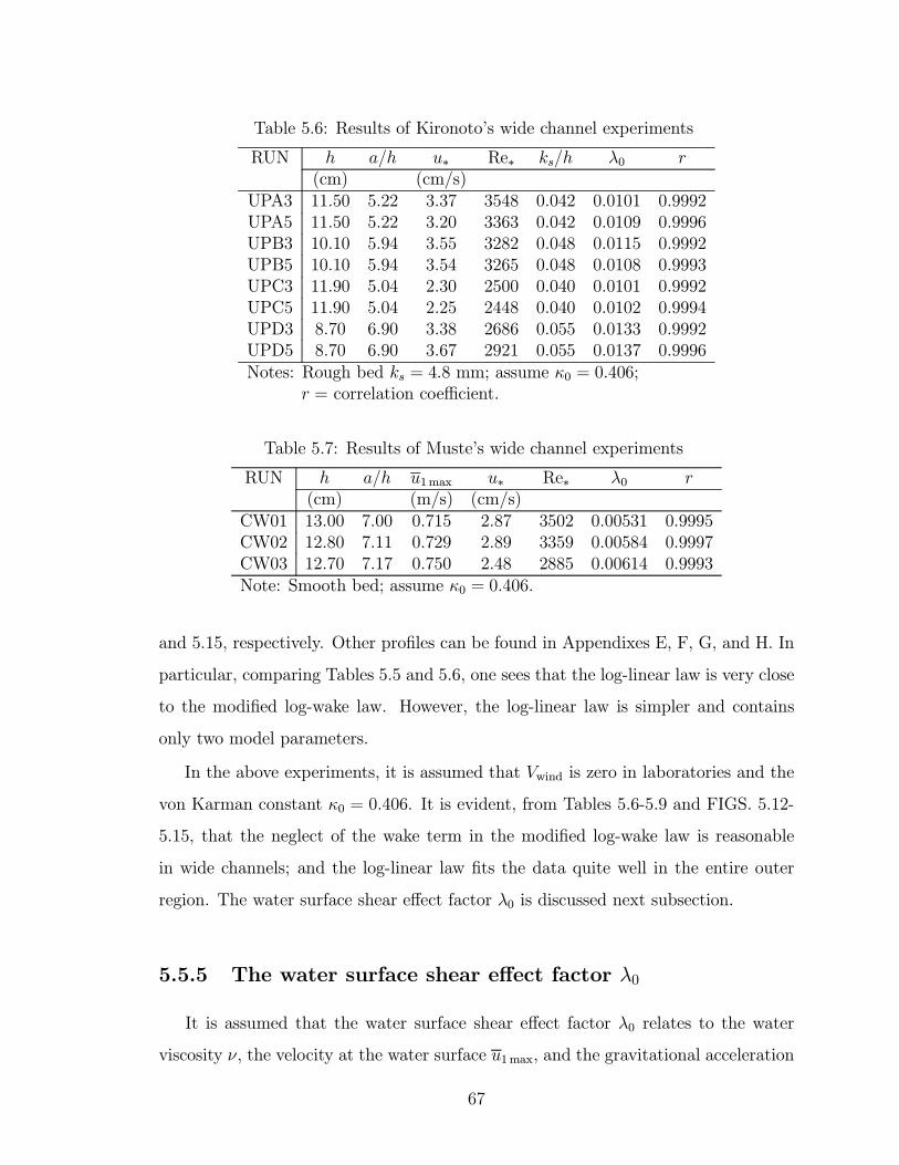
Table 5.6: Results of Kironotos wide channel experiments
RUN h a/h u∗ Re∗ ks/h λ0 r(cm) (cm/s)
UPA3 11.50 5.22 3.37 3548 0.042 0.0101 0.9992UPA5 11.50 5.22 3.20 3363 0.042 0.0109 0.9996UPB3 10.10 5.94 3.55 3282 0.048 0.0115 0.9992UPB5 10.10 5.94 3.54 3265 0.048 0.0108 0.9993UPC3 11.90 5.04 2.30 2500 0.040 0.0101 0.9992UPC5 11.90 5.04 2.25 2448 0.040 0.0102 0.9994UPD3 8.70 6.90 3.38 2686 0.055 0.0133 0.9992UPD5 8.70 6.90 3.67 2921 0.055 0.0137 0.9996Notes: Rough bed ks = 4.8 mm; assume κ0 = 0.406;
r = correlation coefficient.
Table 5.7: Results of Mustes wide channel experiments
RUN h a/h u1max u∗ Re∗ λ0 r(cm) (m/s) (cm/s)
CW01 13.00 7.00 0.715 2.87 3502 0.00531 0.9995CW02 12.80 7.11 0.729 2.89 3359 0.00584 0.9997CW03 12.70 7.17 0.750 2.48 2885 0.00614 0.9993Note: Smooth bed; assume κ0 = 0.406.
and 5.15, respectively. Other proÞles can be found in Appendixes E, F, G, and H. In
particular, comparing Tables 5.5 and 5.6, one sees that the log-linear law is very close
to the modiÞed log-wake law. However, the log-linear law is simpler and contains
only two model parameters.
In the above experiments, it is assumed that Vwind is zero in laboratories and the
von Karman constant κ0 = 0.406. It is evident, from Tables 5.6-5.9 and FIGS. 5.12-
5.15, that the neglect of the wake term in the modiÞed log-wake law is reasonable
in wide channels; and the log-linear law Þts the data quite well in the entire outer
region. The water surface shear effect factor λ0 is discussed next subsection.
5.5.5 The water surface shear effect factor λ0
It is assumed that the water surface shear effect factor λ0 relates to the water
viscosity ν, the velocity at the water surface u1max, and the gravitational acceleration
67
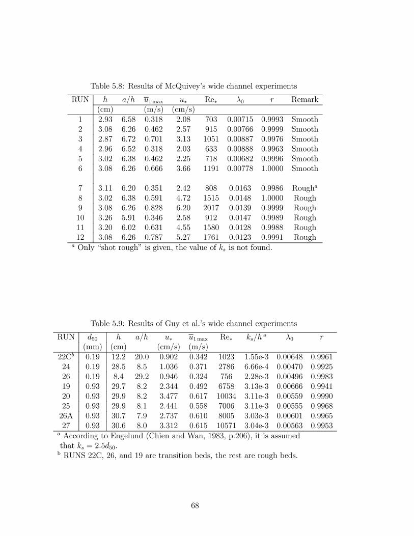
Table 5.8: Results of McQuiveys wide channel experiments
RUN h a/h u1max u∗ Re∗ λ0 r Remark(cm) (m/s) (cm/s)
1 2.93 6.58 0.318 2.08 703 0.00715 0.9993 Smooth2 3.08 6.26 0.462 2.57 915 0.00766 0.9999 Smooth3 2.87 6.72 0.701 3.13 1051 0.00887 0.9976 Smooth4 2.96 6.52 0.318 2.03 633 0.00888 0.9963 Smooth5 3.02 6.38 0.462 2.25 718 0.00682 0.9996 Smooth6 3.08 6.26 0.666 3.66 1191 0.00778 1.0000 Smooth
7 3.11 6.20 0.351 2.42 808 0.0163 0.9986 Rougha
8 3.02 6.38 0.591 4.72 1515 0.0148 1.0000 Rough9 3.08 6.26 0.828 6.20 2017 0.0139 0.9999 Rough10 3.26 5.91 0.346 2.58 912 0.0147 0.9989 Rough11 3.20 6.02 0.631 4.55 1580 0.0128 0.9988 Rough12 3.08 6.26 0.787 5.27 1761 0.0123 0.9991 Rough
a Only shot rough is given, the value of ks is not found.
Table 5.9: Results of Guy et al.s wide channel experiments
RUN d50 h a/h u∗ u1max Re∗ ks/ha λ0 r
(mm) (cm) (cm/s) (m/s)22Cb 0.19 12.2 20.0 0.902 0.342 1023 1.55e-3 0.00648 0.996124 0.19 28.5 8.5 1.036 0.371 2786 6.66e-4 0.00470 0.992526 0.19 8.4 29.2 0.946 0.324 756 2.28e-3 0.00496 0.998319 0.93 29.7 8.2 2.344 0.492 6758 3.13e-3 0.00666 0.994120 0.93 29.9 8.2 3.477 0.617 10034 3.11e-3 0.00559 0.999025 0.93 29.9 8.1 2.441 0.558 7006 3.11e-3 0.00555 0.996826A 0.93 30.7 7.9 2.737 0.610 8005 3.03e-3 0.00601 0.996527 0.93 30.6 8.0 3.312 0.615 10571 3.04e-3 0.00563 0.9953
a According to Engelund (Chien and Wan, 1983, p.206), it is assumedthat ks = 2.5d50.b RUNS 22C, 26, and 19 are transition beds, the rest are rough beds.
68
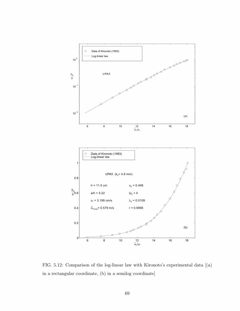
Data of Kironoto (1993)
Log-linear law
6 8 10 12 14 16 18
10 -2
10 -1
10 0
u−1/u *
x3
δ___ UPA5
(a)
Data of Kironoto (1993)Log-linear law
6 8 10 12 14 16 180
0.2
0.4
0.6
0.8
1
u−1/u*
x3
δ___
UPA5 (ks= 4.8 mm)
h = 11.5 cm
a/h = 5.22
u* = 3.199 cm/s
u1max= 0.579 m/s
κ0 = 0.406
Ω0 = 0
λ0 = 0.0109
r = 0.9996
(b)
FIG. 5.12: Comparison of the log-linear law with Kironotos experimental data [(a)
in a rectangular coordinate, (b) in a semilog coordinate]
69
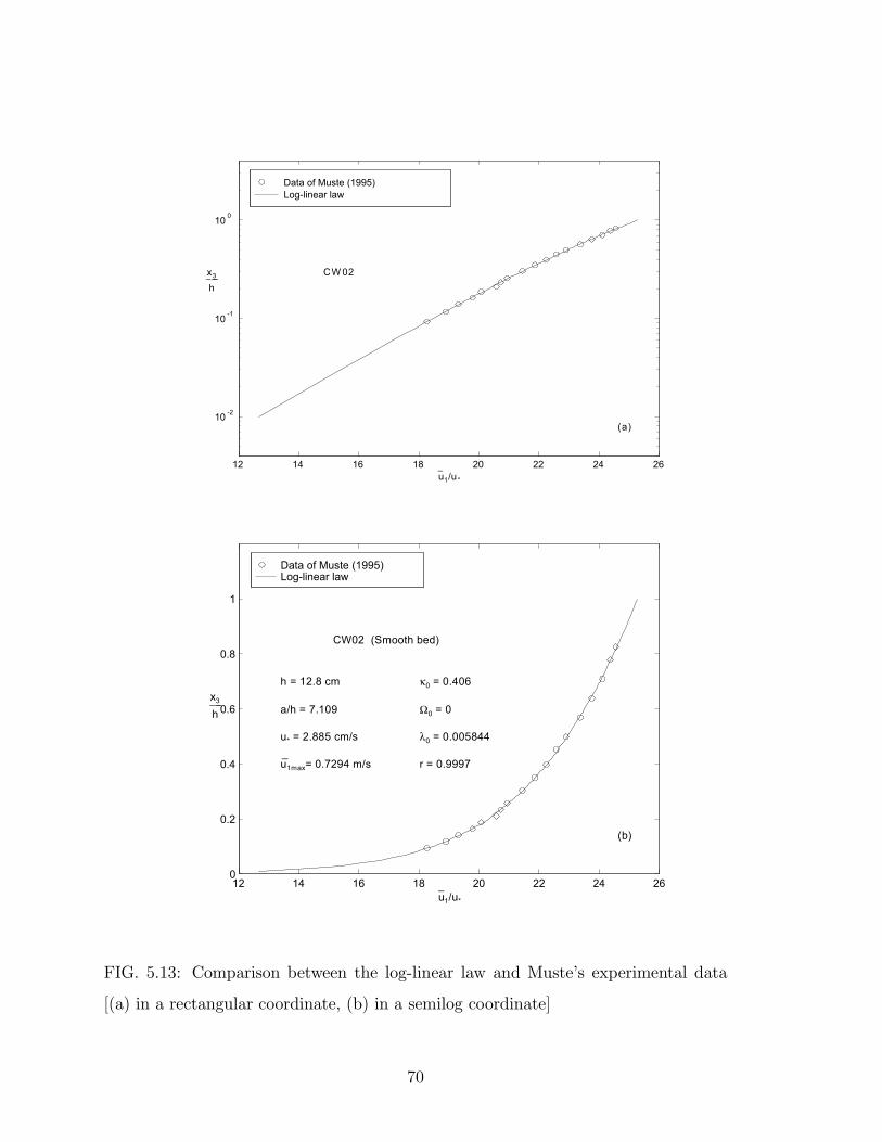
Data of Muste (1995)Log-linear law
12 14 16 18 20 22 24 26
10 -2
10 -1
10 0
u−1/u*
x3
h___ CW 02
(a)
Data of Muste (1995)Log-linear law
12 14 16 18 20 22 24 260
0.2
0.4
0.6
0.8
1
u−1/u*
x3
h___
CW02 (Smooth bed)
h = 12.8 cm
a/h = 7.109
u* = 2.885 cm/s
u1max= 0.7294 m/s
κ0 = 0.406
Ω0 = 0
λ0 = 0.005844
r = 0.9997
(b)
FIG. 5.13: Comparison between the log-linear law and Mustes experimental data
[(a) in a rectangular coordinate, (b) in a semilog coordinate]
70
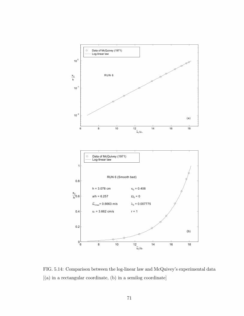
Data of McQuivey (1971)Log-linear law
6 8 10 12 14 16 18
10 -2
10 -1
10 0
u−1/u *
x3
h___ RUN 6
(a)
Data of McQuivey (1971)Log-linear law
6 8 10 12 14 16 180
0.2
0.4
0.6
0.8
1
u−1/u*
x3
h___
RUN 6 (Smooth bed)
h = 3.078 cm
a/h = 6.257
u1max= 0.6663 m/s
u* = 3.662 cm/s
κ0 = 0.406
Ω0 = 0
λ0 = 0.007775
r = 1
(b)
FIG. 5.14: Comparison between the log-linear law and McQuiveys experimental data
[(a) in a rectangular coordinate, (b) in a semilog coordinate]
71
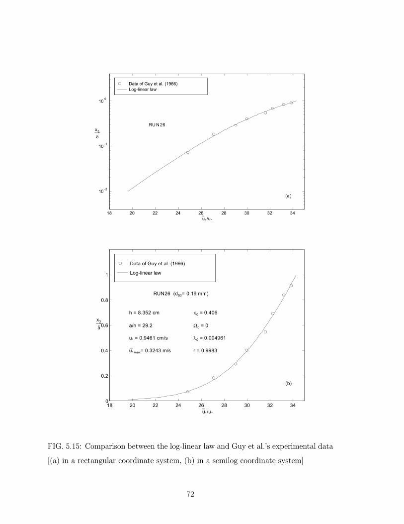
Data of Guy et al. (1966)Log-linear law
18 20 22 24 26 28 30 32 34
10 -2
10 -1
10 0
u−1/u *
x3
δ___
RU N 26
(a)
Data of Guy et al. (1966)
Log-linear law
18 20 22 24 26 28 30 32 340
0.2
0.4
0.6
0.8
1
u−1/u*
x3
δ___
RUN26 (d50= 0.19 mm)
h = 8.352 cm
a/h = 29.2
u* = 0.9461 cm/s
u1max= 0.3243 m/s
κ0 = 0.406
Ω0 = 0
λ0 = 0.004961
r = 0.9983
(b)
FIG. 5.15: Comparison between the log-linear law and Guy et al.s experimental data
[(a) in a rectangular coordinate system, (b) in a semilog coordinate system]
72
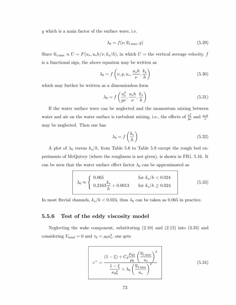
g which is a main factor of the surface wave, i.e.
λ0 = f(ν, u1max, g) (5.29)
Since u1max ∝ U = F (u∗, u∗h/ν, ks/h), in which U = the vertical average velocity, fis a functional sign, the above equation may be written as
λ0 = f
µν, g, u∗,
u∗hν,ksh
¶(5.30)
which may further be written as a dimensionless form
λ0 = f
µu3∗gν,u∗hν,ksh
¶(5.31)
If the water surface wave can be neglected and the momentum mixing between
water and air on the water surface is turbulent mixing, i.e., the effects of u3∗gνand u∗h
ν
may be neglected. Then one has
λ0 = f
µksh
¶(5.32)
A plot of λ0 versus ks/h, from Table 5.6 to Table 5.9 except the rough bed ex-
periments of McQuivey (where the roughness is not given), is shown in FIG. 5.16. It
can be seen that the water surface effect factor λ0 can be approximated as
λ0 ≈(0.065 for ks/h < 0.024
0.2163ksh+ 0.0013 for ks/h ≥ 0.024 (5.33)
In most ßuvial channels, ks/h < 0.024, thus λ0 can be taken as 0.065 in practice.
5.5.6 Test of the eddy viscosity model
Neglecting the wake component, substituting (2.10) and (2.12) into (3.33) and
considering Vwind = 0 and τ0 = ρ0u2∗, one gets
ε+ =(1− ξ) + Cdρair
ρ0
µu1maxu∗
¶21− ξκ0ξ
+ λ0
µu1maxu∗
¶2 (5.34)
73
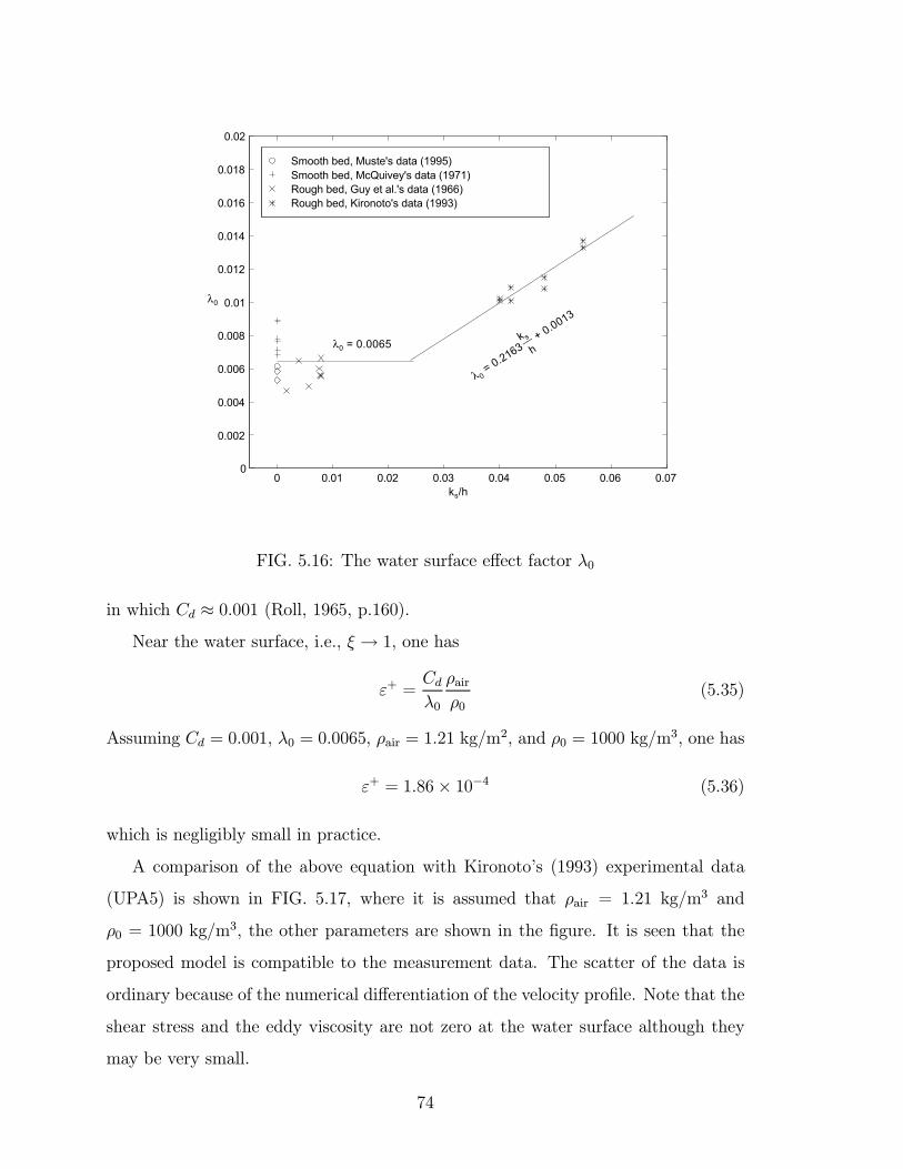
Smooth bed, Muste's data (1995) Smooth bed, McQuivey's data (1971) Rough bed, Guy et al.'s data (1966)Rough bed, Kironoto's data (1993)
0 0.01 0.02 0.03 0.04 0.05 0.06 0.070
0.002
0.004
0.006
0.008
0.01
0.012
0.014
0.016
0.018
0.02
ks/h
λ0
λ0 = 0.0065
λ 0 = 0.2163
k s
h__ + 0.0013
FIG. 5.16: The water surface effect factor λ0
in which Cd ≈ 0.001 (Roll, 1965, p.160).Near the water surface, i.e., ξ → 1, one has
ε+ =Cdλ0
ρairρ0
(5.35)
Assuming Cd = 0.001, λ0 = 0.0065, ρair = 1.21 kg/m2, and ρ0 = 1000 kg/m
3, one has
ε+ = 1.86× 10⁻⁴ (5.36)
which is negligibly small in practice.
A comparison of the above equation with Kironotos (1993) experimental data
(UPA5) is shown in FIG. 5.17, where it is assumed that ρair = 1.21 kg/m3 and
ρ0 = 1000 kg/m3, the other parameters are shown in the Þgure. It is seen that the
proposed model is compatible to the measurement data. The scatter of the data is
ordinary because of the numerical differentiation of the velocity proÞle. Note that the
shear stress and the eddy viscosity are not zero at the water surface although they
may be very small.
74
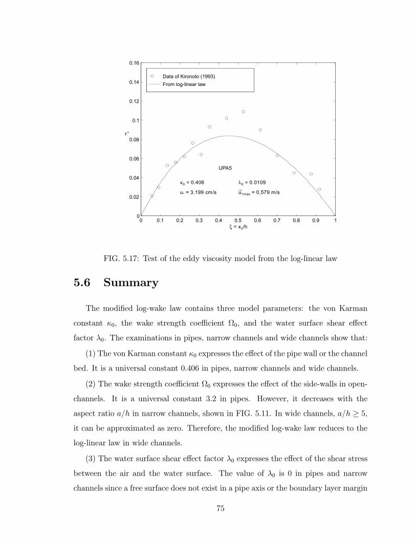
Data of Kironoto (1993)From log-linear law
0 0.1 0.2 0.3 0.4 0.5 0.6 0.7 0.8 0.9 10
0.02
0.04
0.06
0.08
0.1
0.12
0.14
0.16
UPA5
u* = 3.199 cm/s
κ0 = 0.406
u1max = 0.579 m/s
λ0 = 0.0109
ξ = x3/h
ε+
FIG. 5.17: Test of the eddy viscosity model from the log-linear law
5.6 Summary
The modiÞed log-wake law contains three model parameters: the von Karman
constant κ0, the wake strength coefficient Ω0, and the water surface shear effect
factor λ0. The examinations in pipes, narrow channels and wide channels show that:
(1) The von Karman constant κ0 expresses the effect of the pipe wall or the channel
bed. It is a universal constant 0.406 in pipes, narrow channels and wide channels.
(2) The wake strength coefficient Ω0 expresses the effect of the side-walls in open-
channels. It is a universal constant 3.2 in pipes. However, it decreases with the
aspect ratio a/h in narrow channels, shown in FIG. 5.11. In wide channels, a/h ≥ 5,it can be approximated as zero. Therefore, the modiÞed log-wake law reduces to the
log-linear law in wide channels.
(3) The water surface shear effect factor λ0 expresses the effect of the shear stress
between the air and the water surface. The value of λ0 is 0 in pipes and narrow
channels since a free surface does not exist in a pipe axis or the boundary layer margin
75
in a narrow channel. The value of λ0 is almost a constant 0.065 for smooth beds and
small roughness but increases with the relative roughness ks/h when ks/h ≥ 0.024,
see FIG. 5.16.
(4) The modiÞed log-wake law compares very well with experiments in pipes,
narrow channels and wide channels.
(5) The log-linear law, which is the reduction of the modiÞed log-wake law, com-
pares quite well with experiments in wide channels.
(6) The eddy viscosity models (5.11) and (5.34) from the modiÞed log-wake law
and the log-linear law are compatible to experimental data in popes, narrow channels
and wide channels.
76
Chapter 6
THEORETICAL ANALYSIS OF
SEDIMENT-LADEN FLOWS
6.1 Introduction
In the study of clear water ßow, the governing equations are not used at all. The
modiÞed log-wake law is simply based on a similarity analysis. However, a similarity
analysis may not be very helpful in the study of sediment-laden ßows since more
variables are involved. To study the velocity proÞles in sediment-laden ßows, one
may start with the governing equations.
Section 6.2 treats of the governing equations in sediment-laden ßows. Section
6.3 discusses the applications of the governing equations in steady uniform 2D ßows.
Sections 6.4 and 6.5 discuss the effects of sediment suspension. Section 6.6 discusses
sediment-laden velocity proÞles. Section 6.7 summaries the results of this chapter.
6.2 Governing equations
6.2.1 Navier-Stokes equations in sediment-laden ßows
This study aims at the mean velocity proÞles in steady uniform 2D sediment-
laden ßows. However, the turbulent shear stress is signiÞcantly affected by turbulence
77
intensity. To emphasize the effects of sediment suspension on turbulence intensity,
this study starts with unsteady 3D governing equations. To simplify the analysis,
the Boussinesq approximation (Spiegel and Veronis, 1960; Kundu, 1990, p.113)
on stratiÞed ßows is introduced, i.e., the effect of sediment concentration on the ßuid
density may be neglected in the continuity and the momentum equations, except in
the gravity term. The viscosity is also assumed constant in this assumption.
Continuity equation
Based on the Boussinesq assumption, the continuity equation in sediment-laden
ßows is the same as that in clear water, i.e.
∂ui∂xi
= 0 (6.1)
in which ui is the velocity component in the xi direction and i = 1, 2, and 3.
Momentum equation
Similarly, the momentum equation in sediment-laden ßows is written as
∂ui∂t+ uj
∂ui∂xj
=ρ
ρmgi − 1
ρm
∂p
∂xi+ νm
∂2ui∂xj∂xj
(6.2)
in which t is time; j is a dummy subscript; ρ is local density and varies with sediment
concentration; ρm is the (constant) space average of density ρ, i.e. ρm =1V
RVρ dV ;
gi is the component of the gravitational acceleration in the xi direction; p is pressure;
and νm is the (constant) kinematic viscosity corresponding to ρm.
Sediment concentration equation
Applying the mass conservation law to sediment phase, one has the sediment
concentration equation as
∂C
∂t+ uj
∂C
∂xj=
∂
∂xj
µD∂C
∂xj
¶(6.3)
in which C is the sediment volumetric concentration; the Þrst term on the left-hand
side is the concentration change with time; uj , which is not necessary to be the
78
same as that in (6.2), is the convective velocity of sediment; the second term on the
left-hand side is the transport by convection; D is the (constant) molecular diffusion
coefficient; and the right-hand side is the transport by molecular diffusion.
State equation or density equation
The density equation can be easily written as
ρ = ρ0 + (ρs − ρ0)C (6.4)
in which ρ0 is the clear water density; and ρs is the sediment density.
The above equation set (6.1-6.4) is closed since one has 6 equations (1 continuity,
3 momentum, 1 concentration and 1 density equation) with 6 unknowns (3 velocity
components ui, 1 pressure p, 1 density ρ, and 1 concentration C). However, like any
other turbulence, the above equations are very difficult to solve for large Reynolds
number ßows, i.e., turbulent ßows. To study the mean velocity Þeld of a turbulent
ßow, the Reynolds average method may be applied.
6.2.2 Reynolds mean equations and turbulent equations in
sediment-laden ßows
Following Reynolds, one must decompose a variable into its (time) mean part
denoted with an overbar, and a turbulent part denoted with a prime, i.e.
ui = ui + u0i p = p+ p0
ρ = ρ+ ρ0 C = C + C 0(6.5)
Substituting (6.5) into (6.1-6.4) and introducing the Reynolds average method, one
can get the motion equations for the mean ßow and the turbulent ßow, respectively.
Continuity equation
Substituting the expressions (6.5) into (6.1) and taking the Reynolds average, one
has∂ui∂xi
= 0 (6.6)
79
for the mean motion, and∂u0i∂xi
= 0 (6.7)
for the turbulent motion.
From the above two continuity equations, one can get the following two identities:
uj∂f
∂xj=∂(ujf)
∂xju0j∂f
∂xj=∂(u0jf)∂xj
(6.8)
in which f can be any variable. These two identities will be frequently used in the
derivations later.
Momentum equation
Substituting (6.5) into (6.2), one gets
∂(ui + u0i)
∂t+ (uk + u
0k)∂(ui + u
0i)
∂xk=ρ+ ρ0
ρmgi − 1
ρm
∂(p+ p0)∂xi
+ νm∂2
∂xk∂xk(ui + u
0i)
in which ρm =1V
RVρ dV . Applying the identities (6.8) to the convective term and
expanding it, one obtains
∂(ui + u0i)
∂t+∂(uiuk + uiu
0k + u
0iuk + u
0iu0k)
∂xk
=ρ+ ρ0
ρmgi − 1
ρm
∂(p+ p0)∂xi
+ νm∂2
∂xk∂xk(ui + u
0i) (6.9)
Taking the average over this equation and considering that the average of a ßuctuating
variable is zero, one has the following mean motion equation for sediment-laden ßow:
∂ui∂t+∂(uiuk + u0iu
0k)
∂xk=ρ
ρmgi − 1
ρm
∂p
∂xi+ νm
∂2ui∂xk∂xk
(6.10)
or∂ui∂t+ uk
∂ui∂xk
=ρ
ρmgi − 1
ρm
∂p
∂xi+ νm
∂2ui∂xk∂xk
− ∂u0iu0k
∂xk(6.11)
in which u0iu0k is the one-point turbulent velocity correlation. The product of ρm and
−u0iu0k is the so-called turbulent stress or Reynolds stress. (6.11) will be used to studythe mean velocity proÞles in sediment-laden ßows.
The subtraction of the mean motion equation (6.10) from the total motion equa-
tion (6.9) gives the turbulent motion equation, i.e.
∂u0i∂t+∂(uiu
0k + u
0iuk + u
0iu0k − u0iu0k)
∂xk=ρ0
ρmgi − 1
ρm
∂p0
∂xi+ νm
∂2u0i∂xk∂xk
80
or
∂u0i∂t+ u0k
∂ui∂xk
+ uk∂u0i∂xk
+∂u0iu
0k
∂xk− ∂u
0iu0k
∂xk=ρ0
ρmgi − 1
ρm
∂p0
∂xi+ νm
∂2u0i∂xk∂xk
(6.12)
This equation will serve to analyze the effects of sediment suspension on turbulence
intensity.
Sediment concentration equation
Applying (6.5) to (6.3) yields
∂¡C + C 0
¢∂t
+ (uj + u0j)∂¡C + C 0
¢∂xj
=∂
∂xj
ÃD∂¡C + C 0
¢∂xj
!or
∂C
∂t+∂C 0
∂t+ uj
∂C
∂xj+ uj
∂C 0
∂xj+ u0j
∂C
∂xj+∂u0jC
0
∂xj=
∂
∂xj
ÃD∂¡C + C 0
¢∂xj
!(6.13)
Taking the average over this equation gives the mean concentration equation:
∂C
∂t+ uj
∂C
∂xj=
∂
∂xj
µD∂C
∂xj− u0jC 0
¶(6.14)
Similarly, the subtraction of (6.14) from (6.13) gives the turbulent concentration
equation:
∂C 0
∂t+ uj
∂C 0
∂xj+ u0j
∂C
∂xj+∂u0jC
0
∂xj− ∂u
0jC
0
∂xj=
∂
∂xj
µD∂C 0
∂xj
¶(6.15)
State equation or density equation
Applying (6.5) to (6.4) results in
ρ+ ρ0 = ρ0 + (ρs − ρ0)¡C + C 0
¢(6.16)
Taking the average over this equation gives the (time) mean density equation:
ρ = ρ0 + (ρs − ρ0)C (6.17)
Note that this mean density varies with space and has the relation with the space
mean ρm as: ρm =RVρ dV .
Similarly, one can obtain the turbulent density equation:
ρ0 = (ρs − ρ0)C 0 (6.18)
81
Summary
In brief, the mean motion equations for sediment-laden ßows can be summarized
as follows:∂ui∂xi
= 0 (6.6)
∂ui∂t+ uk
∂ui∂xk
=ρ
ρmgi − 1
ρm
∂p
∂xi+ νm
∂2ui∂xk∂xk
− ∂u0iu0k
∂xk(6.11)
∂C
∂t+ uj
∂C
∂xj=
∂
∂xj
µD∂C
∂xj− u0jC 0
¶(6.14)
ρ = ρ0 + (ρs − ρ0)C (6.17)
To solve this set of equations, one must make some assumptions about u0iu0k and u
0jC
0.
This is known as the closure problem.
The turbulent motion equations are summarized as
∂u0i∂xi
= 0 (6.7)
∂u0i∂t+ u0k
∂ui∂xk
+ uk∂u0i∂xk
+∂u0iu
0k
∂xk− ∂u
0iu0k
∂xk=ρ0
ρmgi − 1
ρm
∂p0
∂xi+ νm
∂2u0i∂xk∂xk
(6.12)
∂C 0
∂t+ uj
∂C 0
∂xj+ u0j
∂C
∂xj+∂u0jC
0
∂xj− ∂u
0jC
0
∂xj=
∂
∂xj
µD∂C 0
∂xj
¶(6.15)
ρ0 = (ρs − ρ0)C 0 (6.18)
Only (6.12) of this set will be used to study the effects of sediment suspension on
turbulence intensity.
6.3 SimpliÞcations of governing equations in steady
uniform 2D ßows
To simplify the analysis, this study assumes that the mean ßow is 2D steady
uniform, shown in FIG. 6.1. That is,
steady :∂( )
∂t= 0 (6.19)
uniform :∂( )
∂x1= 0,
∂( )
∂x2= 0 (6.20)
2D ßow : u1 = u1(x3), u2 = u3 = 0, C = C(x3) (6.21)
82
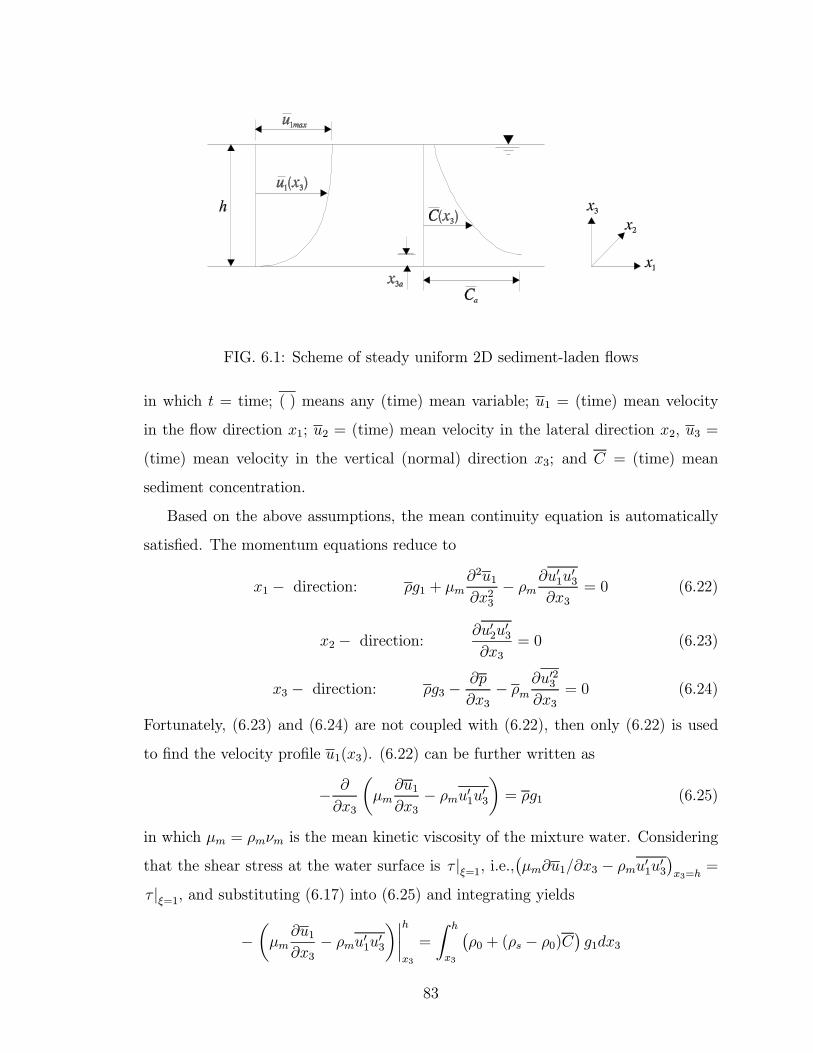
FIG. 6.1: Scheme of steady uniform 2D sediment-laden ßows
in which t = time; ( ) means any (time) mean variable; u1 = (time) mean velocity
in the ßow direction x1; u2 = (time) mean velocity in the lateral direction x2, u3 =
(time) mean velocity in the vertical (normal) direction x3; and C = (time) mean
sediment concentration.
Based on the above assumptions, the mean continuity equation is automatically
satisÞed. The momentum equations reduce to
x1 − direction: ρg1 + µm∂2u1∂x23
− ρm∂u01u03
∂x3= 0 (6.22)
x2 − direction:∂u02u03∂x3
= 0 (6.23)
x3 − direction: ρg3 − ∂p
∂x3− ρm
∂u023∂x3
= 0 (6.24)
Fortunately, (6.23) and (6.24) are not coupled with (6.22), then only (6.22) is used
to Þnd the velocity proÞle u1(x3). (6.22) can be further written as
− ∂
∂x3
µµm∂u1∂x3
− ρmu01u03¶= ρg1 (6.25)
in which µm = ρmνm is the mean kinetic viscosity of the mixture water. Considering
that the shear stress at the water surface is τ |ξ=1, i.e.,¡µm∂u1/∂x3 − ρmu01u03
¢x3=h
=
τ |ξ=1, and substituting (6.17) into (6.25) and integrating yields
−µµm∂u1∂x3
− ρmu01u03¶¯h
x3
=
Z h
x3
¡ρ0 + (ρs − ρ0)C
¢g1dx3
83
or
µm∂u1∂x3
− ρmu01u03 − τ |ξ=1 = ρ0g1 (h− x3) + (ρs − ρ0)g1Z h
x3
Cdx3 (6.26)
Now one can see that the effects of sediment suspension on velocity proÞles may be
in three ways: (1) changing the ßuid viscosity µm and then changing the viscous shear
stress (1st term on the left-hand side); (2) changing the ßuid density and turbulence
intensity and consequently changing the turbulent shear stress (2nd term on the
left-hand side); and (3) producing density gradient and then increasing the gravity
component in the ßow direction (2nd term on the right-hand side). To further simplify
(6.26), a magnitude order for each term in (6.26) is analyzed as follows:
By experience, one may assume
u1 ∼ U , x3 ∼ h, u01u03 ∼ u2∗, C ∼ Ca, ρm ∼ ρ0
in which U is the vertical average velocity; u∗ is the shear velocity; and Ca is a near
bed concentration, then one has:
µm∂u1∂x3
−ρmu01u03 − τ |ξ=1 = ρ0g1h −ρ0g1x3 +(ρs − ρ0)g1R hx3Cdx3
µmU
hρmu
2∗ Keep ρ0g1h ρ0g1h (ρs − ρ0)g1hCa
Divided by ρmU2
µmρmUh
³u∗U
´2Keep
ρ0ρm
g1h
U2ρ0ρm
g1h
U2ρs − ρ0ρm
g1h
U2Ca
Since u∗ =√ghS =
√g1h, and ρm ∼ ρ0, one has
1
Re
³u∗U
´2Keep
³u∗U
´2 ³u∗U
´2 ρs − ρ0ρm
³u∗U
´2Ca
Multiplying (U/u∗)2:
1
Re
µU
u∗
¶21 Keep 1 1
ρs − ρ0ρm
Ca
In practice, Re > 104, Uu∗ ∼ 10, and let ρs−ρ0ρm
Ca < 0.1
< 0.01 1 Keep 1 1 < 0.1
84
The above magnitude order analysis shows that the main effects of sediment sus-
pension on the mean velocity proÞles are by the turbulent shear stress. In other
words, the momentum equation in steady uniform 2D sediment-laden ßows can be
further simpliÞed as
−ρmu01u03 − τ |ξ=1 = ρ0g1 (h− x3) (6.27)
Note that τ |ξ=1 is kept in the above equation since it is the derivative boundary condi-tion at the water surface although it may be very small. The above equation is similar
to that in clear water, but the turbulent shear stress must be modiÞed by sediment
suspension. Introducing the eddy viscosity concept, i.e., −u01u03 = ε+u∗hdu1/dx3, inwhich ε+ is the dimensionless eddy viscosity, the above equation becomes
ρmε+u∗h
du1dx3
− τ |ξ=1 = ρ0g1 (h− x3) (6.28)
Furthermore, if one deÞnes ε+m = (ρm/ρ0)ε+ as the dimensionless eddy viscosity in
sediment-laden ßows, then one obtains
ρ0ε+mu∗h
du1dx3
− τ |ξ=1 = ρ0g1 (h− x3) (6.29)
The above equation is exactly the same as that in clear water except that the eddy
viscosity is modiÞed by sediment suspension.
Note that the assumption of (ρs−ρ0)/ρmCa < 0.1 means that for plastic sediments(speciÞc gravity G = 1.05), Ca can be very large; for natural sediments (G = 2.65),
Ca < 0.1. When Ca ≥ 0.1 in natural sediment-laden ßows, the effect of sediment
suspension on the gravity must be included.
Similarly, for steady uniform 2D ßows, the sediment concentration equation (6.14)
reduces to
−ω ∂C∂x3
=∂
∂x3
µD∂C
∂x3− u03C 0
¶(6.30)
in which u3 = −ω, where ω is sediment settling velocity. Integrating (6.30) gives that
D∂C
∂x3− u03C 0 + ωC = const
85
Considering that no sediments enter into ßow from the water surface, one has
D∂C
∂x3− u03C 0 + ωC = 0
Usually the molecular diffusion ßux of sediment is much smaller than the turbulent
ßux, i.e., the above equation may be simpliÞed as
−u03C 0 + ωC = 0 (6.31)
According to Reynolds analogy, introducing −u03C 0 = ε+s u∗hdC/dx3, in which ε+s isthe turbulent sediment diffusion coefficient, the above equation becomes
ε+s u∗hdC
dx3+ ωC = 0 (6.32)
Equations (6.29) and (6.32) constitute the governing equations in steady uniform
2D sediment-laden ßows. The eddy viscosity models from clear water, i.e., (5.11) for
narrow channels and (5.34) for wide channels, may be used for the problem closure.
Again, the effects of the sediment suspension on the eddy viscosity models must be
considered.
6.4 Effects of sediment suspension on turbulence
intensities
Sediment suspension is due to turbulent kinetic energy. The eddy viscosity ε in
the vertical direction relates to a characteristic length scale and the vertical turbu-
lence intensity u03. The larger the turbulence intensity u03, the stronger the turbulent
diffusion or mixing, i.e.
ε ∼ δ u03 (6.33)
in which δ is the boundary layer thickness (characteristic length scale). For wide
channels, δ = h. Hence, the study of the effects of sediment suspension on the
turbulence intensities (the kinetic energy budget and the eddy viscosity) is important.
86
6.4.1 Turbulence intensity u0iu0j in sediment-laden ßows
One may start with (6.12), the equation for the turbulent velocity component u0i.
One can also write the same equation for the velocity component u0j . Multiplying the
equation for u0i by u0j and the equation for u
0j by u
0i, one gets
u0j∂u0i∂t+ u0ju
0k
∂ui∂xk
+ u0juk∂u0i∂xk
+ u0j∂(u0iu
0k − u0iu0k)∂xk
=u0jρ
0
ρmgi −
u0jρm
∂p0
∂xi+ νmu
0j
∂2u0i∂xk∂xk
and
u0i∂u0j∂t
+ u0iu0k
∂uj∂xk
+ u0iuk∂u0j∂xk
+ u0i∂(u0ju
0k − u0ju0k)∂xk
=u0iρ
0
ρmgj − u0i
ρm
∂p0
∂xj+ νmu
0i
∂2u0j∂xk∂xk
Adding the above two equations gives
∂u0iu0j
∂t+ u0ju
0k
∂ui∂xk
+ u0iu0k
∂uj∂xk
+ uk∂u0iu
0j
∂xk+ u0j
∂(u0iu0k − u0iu0k)∂xk
+ u0i∂(u0ju
0k − u0ju0k)∂xk
=u0jρ
0
ρmgi +
u0iρ0
ρmgj −
u0jρm
∂p0
∂xi− u0iρm
∂p0
∂xj+ νm
µu0j
∂2u0i∂xk∂xk
+ u0i∂2u0j∂xk∂xk
¶The average over this equation yields the correlation equation of u0iu
0j, i.e.
∂u0iu0j
∂t+ u0ju
0k
∂ui∂xk
+ u0iu0k
∂uj∂xk
+ uk∂u0iu
0j
∂xk
= −Ãu0j∂u0iu
0k
∂xk+ u0i
∂u0ju0k
∂xk
!+1
ρm
¡u0jρ0gi + u
0iρ0gj¢
− 1
ρm
µu0j∂p0
∂xi+ u0i
∂p0
∂xj
¶+ νm
Ãu0j
∂2u0i∂xk∂xk
+ u0i∂2u0j∂xk∂xk
!(6.34)
The terms on the right-hand side of this equation may be transformed to measurable
forms.
Applying the identities (6.8), the stuff within the bracket of the Þrst term on the
right-hand side becomes
u0j∂u0iu
0k
∂xk+ u0i
∂u0ju0k
∂xk= u0ju
0k
∂u0i∂xk
+ u0i∂u0ju
0k
∂xk=∂u0iu
0ju0k
∂xk(6.35)
Considering (6.18), the stuff within the bracket of the second term on the right-hand
side becomes
u0jρ0gi + u0iρ0gj = (ρs − ρ0)
¡u0jC 0gi + u
0iC
0gj¢
(6.36)
87
The stuff within the bracket of the third term on the right-hand side may be written
as
u0j∂p0
∂xi+ u0i
∂p0
∂xj=
∂p0u0j∂xi
− p0∂u0j
∂xi+∂p0u0i∂xj
− p0 ∂u0i
∂xj
=
Ã∂p0u0j∂xi
+∂p0u0i∂xj
!− p0
µ∂u0j∂xi
+∂u0i∂xj
¶(6.37)
Since
∂2
∂xk∂xku0iu
0j =
∂
∂xk
µu0i∂u0j∂xk
+ u0j∂u0i∂xk
¶=
∂u0i∂xk
∂u0j∂xk
+ u0i∂2u0j∂xk∂xk
+∂u0j∂xk
∂u0i∂xk
+ u0j∂2u0i∂xk∂xk
= u0i∂2u0j∂xk∂xk
+ u0j∂2u0i∂xk∂xk
+ 2∂u0i∂xk
∂u0j∂xk
one can get the fourth term on the right-hand side as
u0i∂2u0j∂xk∂xk
+ u0j∂2u0i∂xk∂xk
=∂2
∂xk∂xku0iu
0j − 2
∂u0i∂xk
∂u0j∂xk
(6.38)
Substituting (6.35-6.38) into (6.34) yields the one-point velocity correlation equa-
tion:
∂u0iu0j
∂t+ uk
∂u0iu0j
∂xk= −
µu0ju
0k
∂ui∂xk
+ u0iu0k
∂uj∂xk
¶+ρs − ρ0ρm
¡u0jC 0gi + u
0iC
0gj¢
−∂u0iu0ju0k
∂xk− 1
ρm
Ã∂p0u0j∂xi
+∂p0u0i∂xj
!+1
ρmp0µ∂u0j∂xi
+∂u0i∂xj
¶+νm
∂2u0iu0j
∂xk∂xk− 2νm ∂u
0i
∂xk
∂u0j∂xk
(6.39)
This equation is the same as that in clear water (Hinze, 1975, p.324) except an extra
term which relates to sediment suspension. The above equation is the general one-
point velocity correlation equation. It can be used to study any second order velocity
correlations, such as u021 , u01u02, u
01u03, u
022 , u
02u03, u
023 , and turbulent kinetic energy
12u0iu
0i.
In this section, only the turbulent kinetic energy 12u0iu
0i and the vertical turbulence
intensity u023 are concerned since they relate to the Richardson number and the eddy
viscosity in sediment-laden ßows.
88
6.4.2 Turbulent kinetic energy budget and Richardson num-
ber in sediment-laden ßows
To study the turbulent kinetic energy budget, let i = j in (6.39), then one has
∂u0iu0i
∂t= −2u0iu03
∂ui∂x3
+2ρs − ρ0ρm
u0iC 0gi−∂u0iu
0iu03
∂x3− 2
ρm
∂p0u03∂x3
+νm∂2u0iu
0i
∂x3∂x3−2νm ∂u
0i
∂xk
∂u0i∂xk
or
∂
∂t
q2
2= −u01u03
∂u1∂x3| z
turb. production
+ρs − ρ0ρm
u0iC 0gi| z sediment suspension
− ∂
∂x3
µq2
2+p0
ρm
¶u03| z
turbulent transport
+ νm∂2
∂x23
Ãq2
2
!| z viscous transport
− νm∂u0i∂xk
∂u0i∂xk| z
energy dissipation
(6.40)
in which q2 = u0iu0i. The transport by viscous diffusion is usually neglected. The
turbulent transport may also be neglected if the turbulence intensity is not very
strong. This is because p0 ∝ q2 > 0, p0u03 ∝ q2u03 ≈ 0. Thus, (6.40) reduces to∂
∂t
q2
2= −u01u03
∂u1∂x3| z
turb. production
+ρs − ρ0ρm
u0iC 0gi| z sediment suspension
− νm∂u0i∂xk
∂u0i∂xk| z
energy dissipation
(6.41)
Experiments (Vanoni, 1946; Einstein and Chien, 1955; Elata and Ippen, 1961; and
others) have shown that both −u01u03 and ∂u1∂x3
are positive and increase with sediment
suspension. This implies that the effect of sediment suspension on the turbulent
production ampliÞes the turbulent kinetic energy.
Because the concentration Þeld is homogeneous in the x1 and the x2 directions,
the mean turbulent mixing ßuxes in these directions must be zero, i.e.
u01C 0 = u02C 0 = 0 (6.42)
Thus,ρs − ρ0ρm
u0iC 0gi =ρs − ρ0ρm
u03C 0g3
To balance the sediment settling from upward, the turbulent mixing ßux u03C 0 in the
x3 direction must be positive, i.e.
u03C 0 > 0 (6.43)
89
Considering g3 = −g cos θ ≈ −g (in which θ is the angle between the channel bedand the datum), one has
ρs − ρ0ρm
u03C 0g3 < 0 (6.44)
which implies that sediment suspension decreases the turbulent kinetic energy. In
other words, the energy supported suspended-load comes from the turbulent kinetic
energy rather than the mean ßow energy.
Since sediment presence increases the viscosity νm, it is expected that the energy
dissipation increases in sediment-laden ßow.
Of all three terms on the right-hand side in (6.41), two of them are negative
(sediment suspension + energy dissipation) and one (turbulent production) is positive,
the resultant of the right-hand side may increase and may decrease the turbulent
kinetic energy. However, in any case, sediment suspension will increase the mean
ßow energy loss. This is because sediment suspension increases turbulent production
which, in turn, comes from the mean ßow energy.
The Richardson number Ri is deÞned as the ratio of the sediment suspension
energy to the turbulent production in (6.41), i.e.
Ri =
ρs − ρ0ρm
u03C 0g
−u01u03du1dx3
(6.45)
Introducing
−u01u03 = εmdu1dx3
−u03C 0 = εsdC
dx3
in which the turbulent sediment diffusion coefficient εs is proportional to the momen-
tum eddy viscosity εm. Therefore,
Ri ∝ −(ρs − ρ0)gρm
dC
dx3µdu1dx3
¶290
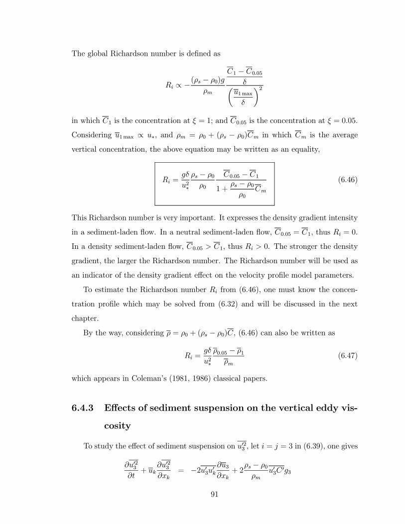
The global Richardson number is deÞned as
Ri ∝ −(ρs − ρ0)gρm
C1 − C0.05δµ
u1maxδ
¶2in which C1 is the concentration at ξ = 1; and C0.05 is the concentration at ξ = 0.05.
Considering u1max ∝ u∗, and ρm = ρ0 + (ρs − ρ0)Cm in which Cm is the average
vertical concentration, the above equation may be written as an equality,
Ri =gδ
u2∗
ρs − ρ0ρ0
C0.05 − C11 +
ρs − ρ0ρ0
Cm
(6.46)
This Richardson number is very important. It expresses the density gradient intensity
in a sediment-laden ßow. In a neutral sediment-laden ßow, C0.05 = C1, thus Ri = 0.
In a density sediment-laden ßow, C0.05 > C1, thus Ri > 0. The stronger the density
gradient, the larger the Richardson number. The Richardson number will be used as
an indicator of the density gradient effect on the velocity proÞle model parameters.
To estimate the Richardson number Ri from (6.46), one must know the concen-
tration proÞle which may be solved from (6.32) and will be discussed in the next
chapter.
By the way, considering ρ = ρ0 + (ρs − ρ0)C, (6.46) can also be written as
Ri =gδ
u2∗
ρ0.05 − ρ1ρm
(6.47)
which appears in Colemans (1981, 1986) classical papers.
6.4.3 Effects of sediment suspension on the vertical eddy vis-
cosity
To study the effect of sediment suspension on u023 , let i = j = 3 in (6.39), one gives
∂u023∂t
+ uk∂u023∂xk
= −2u03u0k∂u3∂xk
+ 2ρs − ρ0ρm
u03C 0g3
91
−∂u03u03u0k
∂xk− 2
ρm
∂p0u03∂x3
+2
ρmp0∂u03∂x3
+νm∂2u023∂x23
− 2νm∂u03
∂xk
∂u03∂xk
(6.48)
Considering (6.20) and (6.21) gives that
uk∂u023∂xk
= 0 (6.49)
Considering u3 = 0 gives that
u03u0k
∂u3∂xk
= 0 (6.50)
Considering (6.20) gives that
∂u03u03u0k∂xk
=∂u033∂x3
(6.51)
Then (6.48) becomes
∂u023∂t
= 2ρs − ρ0ρm
u03C 0g3| z sediment suspension
−∂u033
∂x3− 2
ρm
∂p0u03∂x3
+2
ρmp0∂u03∂x3| z
turbulent transport
+ νm∂2u023∂x23| z
vis. transp.
− 2νm∂u03∂xk
∂u03∂xk| z
energy dissipation
(6.52)
In the following, one will assume a clear water running in a ßume, then add some
sediments to the ßow to see how u023 adjusts according to the right-hand side terms.
Assume that the viscous and the turbulent transport terms are neglected or sec-
ondary. Then the effects of sediment suspension on u023 are mainly through two terms:
sediment suspension and energy dissipation.
As those in (6.41), both the sediment suspension term and the energy dissipation
term are negative. They will damp the turbulence intensity u03. Consequently, sedi-
ment suspension damps the eddy viscosity in the vertical direction. The decrease of
the eddy viscosity weakens turbulent mixing compared with a clear water ßow. In
other words, the outer region (overlap + wake layer + boundary effect layer) velocity
gradient in a sediment-laden ßow increases compared with a clear water ßow.
92
6.5 ModiÞcation of the eddy viscosity model in
sediment-laden ßows
Assume that the structure of the eddy viscosity model (3.33) obtained in clear
water ßows is still valid in sediment-laden ßows. Then the incorporation of the effect
of sediment concentration may be four alternatives:
Alternative 1: To consider the sediment damping effect, following Monin and
Obukhov (Duo, 1987, p.365), a concentration factor Φs may be introduced to the
eddy viscosity expression, i.e.
ε+m =1
Φs
(1− ξ) + τ |ξ=1 /τw1− ξκ0ξ
+πΩ02sin πξ +
1
u∗
du1dξ
¯ξ=1
(6.53)
in which Φs is a function of concentration C , i.e.
Φs = 1 + α1C + α2C2+ · · · (6.54)
where α1 and α2 are experimental constants. In this case, the concentration equation
(6.32) must be coupled with (6.29). Besides, if C is replaced by a characteristic
concentration Ca and if Ca is very small, then sediment concentration will not affect
the von Karman constant κ0 and the wake strength coefficient Ω0. Only an additional
term is added in the clear water velocity proÞle equation, like the Monin-Obukhov
equation in an atmosphere ßow (Kundu, 1990, p.463). Note that the subscript 0
denotes values in clear water.
Alternative 2: Both the von Karman constant κ and the wake strength coefficient
Ω in sediment-laden ßows vary with a characteristic concentration, i.e., the sediment
damping may be considered by decreasing κ and increasing Ω. That is, κ < κ0, and
Ω > Ω0.
Alternative 3: κ may become smaller with a characteristic concentration, i.e.,
κ < κ0, while Ω may keep the same as that in clear water, i.e., Ω = Ω0.
Alternative 4: κ may keep the same as that in clear water, i.e., κ = κ0 = 0.406,
while Ω may increase with a characteristic concentration, i.e., Ω > Ω0.
93
Alternative 1 is cumbersome. Alternatives 2, 3 and 4 are relative simple since
one can choose a near bed concentration or the vertical mean concentration to reßect
the effect of sediment suspension. In this dissertation, only last three alternatives are
examined.
6.6 Velocity proÞles in sediment-laden ßows
Of course, for the last three alternatives, the velocity proÞle equations are similar
to those in clear water except that the von Karman constant κ, the wake strength
coefficient Ω, and the water surface shear effect factor λ may vary with sediment
suspension. That is, the velocity proÞles in narrow channels can still be described
by (5.1), and the velocity proÞles in wide channels can still be expressed by (5.23).
However, one has
κ,Ω,λ = F (characteristic concentration, density gradient)
= F (Ca, Ri) (6.55)
in which Ca = C0.05 for κ and Ca = C1 for Ω and λ. This is because the von Karman
constant is determined by the near bed ßow while the wake strength coefficient Ω and
the water surface shear effect factor λ are determined by the ßow near the boundary
layer margin or the water surface.
6.7 Summary
In this chapter, one starts with the full governing equations in sediment-laden
ßows and obtains the steady uniform 2D governing equations. Based on the turbu-
lent kinetic energy equation, the global Richardson number Ri is derived. Based on
the equation of the turbulence intensity u023 , it is shown that sediment suspension
affects the eddy viscosity in two ways: increasing the molecular viscosity and then
increasing energy dissipation, and losing turbulent energy to support sediment sus-
pension. Both ways will damp the vertical eddy viscosity. Using a magnitude order
94
analysis method, it is shown that the velocity proÞle equation in a sediment-laden
ßow takes the same form as that in clear water, except the model parameters may
vary with a characteristic concentration and density gradient.
95
Chapter 7
TEST OF THE MODIFIED
LOG-WAKE LAW IN
SEDIMENT-LADEN FLOWS
7.1 Introduction
The modiÞed log-wake law has been tested to be true in clear water in Chapter
5. Chapter 6 shows that it may be true for sediment-laden ßows. However, sediment
suspension may modify the parameters κ, Ω and λ. This chapter will test the modiÞed
log-wake law in sediment-laden ßows and study the variations of κ, Ω and λ with
sediment suspension.
Section 7.2 presents a test strategy, i.e., using two extreme experiments to test the
effects of molecular viscosity and density gradient. Sections 7.3 and 7.4 discuss the
effects of sediment suspension on the model parameters in narrow and wide channels.
Section 7.5 summaries the results of this chapter.
7.2 Preliminary analysis of the model parameters
In Chapter 6, one sees that sediment suspension affects the velocity proÞles of
sediment-laden ßows in two ways: one is that sediment concentration increases mole-
96
cular viscosity and then increases energy dissipation and consequently damps tur-
bulence intensity; the other is that to balance sediment settling due to the gravity,
suspended sediments obtain energy from turbulent kinetic energy and then damp
turbulence intensity. These two effects can be examined in two kinds of extreme ex-
periments: one is neutral sediment-laden experiments where the concentration can be
very high, the effect of viscosity is emphasized, but sediment suspension does not cost
turbulent energy at all; the other is density (stratiÞed) sediment-laden experiments
where the concentration keeps so small that the effect of molecular viscosity may be
neglected but the effect of the density gradient is emphasized.
For neutral sediment-laden ßows, C = C0.05 = C1, Ri = 0, then (6.55) reduces to
κ,Ω,λ = F1¡C¢
(7.1)
For density sediment-laden ßows with dilute concentration, the effect of viscosity may
be neglected. Then (6.55) reduces to
κ,Ω,λ = F2 (Ri) (7.2)
(7.1) and (7.2) are two asymptotic expressions. A composite expression for (6.55)
may be expressed as
κ,Ω,λ = F1¡Ca¢+ F2 (Ri)− (κ,Ω,λ)|clear water (7.3)
In the following, one will Þnd the functional forms of F1 and F2 for each parameter
κ, Ω and λ.
7.3 Test of the modiÞed log-wake law in narrow
open-channels
The model parameters in narrow channels include κ and Ω. The plastic particle
experiments by Wang and Qian (1989) will serve to test the effect of molecular vis-
cosity. The sediment experiments by Coleman (1986) will serve to study the effect of
density gradient.
97
7.3.1 Effect of molecular viscosity
Wang and Qian (1989) did three types of experiments: clear water and pure salt
water (see Section 5.3.3), neutral sediment-laden ßows (salt water + plastic parti-
cles), and density sediment-laden ßows (clear water + plastic particles, clear water
+ natural sands). The speciÞc gravity of plastic particles G = 1.05, the particle con-
centration distribution in clear water is close to uniform, so the clear water + plastic
particle experiments can be regarded as quasi-neutral sediment-laden ßows, i.e., the
effect of density gradient may be neglected herein. In the experiments, three sediment
sizes (Þne, middle and coarse) were used, see Appendix C. The ßume perimeters were
kept the same (smooth boundary, ßow depth h = 9 cm, ßume width a = 30 cm, and
bed slope S = 0.01), the differences among individual runs are only attributed to
different concentrations. The maximum volumetric concentration was 20%.
In the following tests, the shear velocity u∗, as it in clear water, is determined by
(4.16) since it is a kinematic variable. The kinematic molecular viscosity νm due to
volumetric sediment concentration is calculated by (Coleman, 1986)
νm =µ(1 + 2.5C + 6.25C
2+ 15.62C
3)
ρ0 + (ρs − ρ0)C(7.4)
in which µ is the kinetic molecular viscosity of water; and C is the volumetric sediment
concentration. The velocity proÞle analysis procedure is the exact same as that in
clear water.
Velocity proÞles
A representative velocity proÞle, along with the modiÞed log-wake law, of neutrally-
buoyant sediment-laden ßows is shown in FIG. 7.1. All other proÞles can be found in
Appendix C. Four velocity proÞles of the Þne particle (medium size d50 = 0.268 mm)
experiments with different concentrations are plotted in FIG. 7.2. From the above
two Þgures, one sees that: (1) The sediment concentration ampliÞes the thickness of
the viscous layer (the viscous sublayer + the buffer layer). The higher the concentra-
tion, the thicker the viscous layer. (2) As the concentration increases, the position of
98
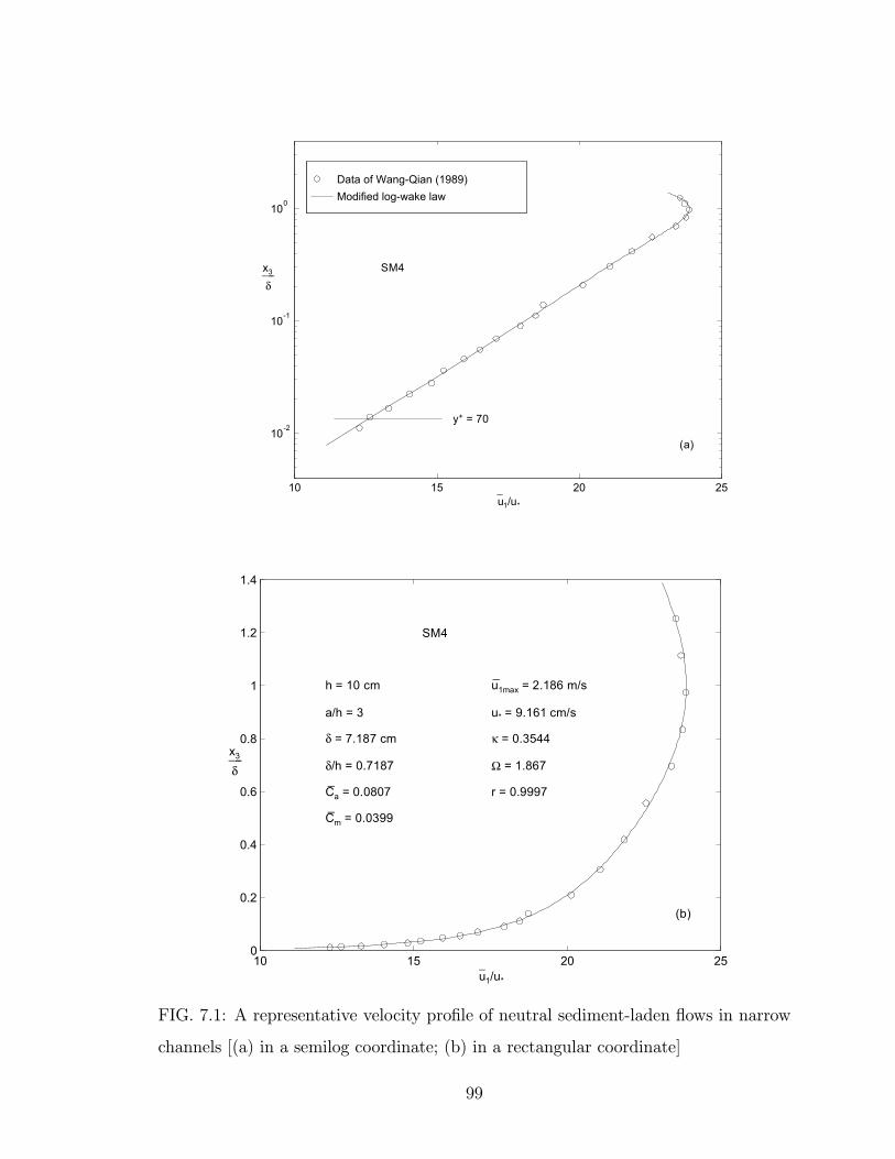
Data of Wang-Qian (1989)Modified log-wake law
10 15 20 25
10-2
10-1
100
u−1/u*
x3
δ___ SM4
(a)
y+ = 70
10 15 20 250
0.2
0.4
0.6
0.8
1
1.2
1.4
u−1/u*
x3
δ___
SM4
h = 10 cm
a/h = 3
δ = 7.187 cm
δ/h = 0.7187
Ca = 0.0807
Cm = 0.0399
u1max = 2.186 m/s
u* = 9.161 cm/s
κ = 0.3544
Ω = 1.867
r = 0.9997
(b)
FIG. 7.1: A representative velocity proÞle of neutral sediment-laden ßows in narrow
channels [(a) in a semilog coordinate; (b) in a rectangular coordinate]
99
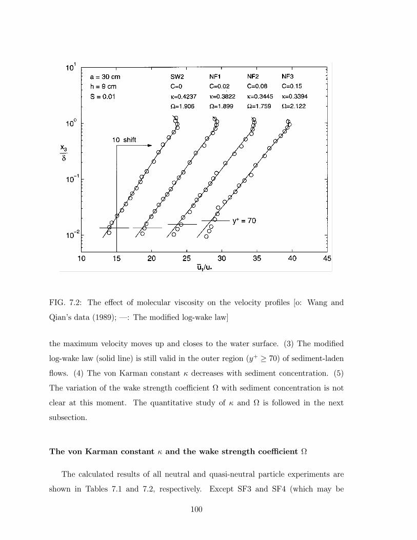
FIG. 7.2: The effect of molecular viscosity on the velocity proÞles [o: Wang and
Qians data (1989); : The modiÞed log-wake law]
the maximum velocity moves up and closes to the water surface. (3) The modiÞed
log-wake law (solid line) is still valid in the outer region (y+ ≥ 70) of sediment-ladenßows. (4) The von Karman constant κ decreases with sediment concentration. (5)
The variation of the wake strength coefficient Ω with sediment concentration is not
clear at this moment. The quantitative study of κ and Ω is followed in the next
subsection.
The von Karman constant κ and the wake strength coefficient Ω
The calculated results of all neutral and quasi-neutral particle experiments are
shown in Tables 7.1 and 7.2, respectively. Except SF3 and SF4 (which may be
100
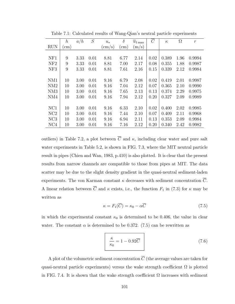
Table 7.1: Calculated results of Wang-Qians neutral particle experiments
h a/h S u∗ δ u1max C κ Ω rRUN (cm) (cm/s) (cm) (m/s)
NF1 9 3.33 0.01 8.81 6.77 2.14 0.02 0.389 1.96 0.9994NF2 9 3.33 0.01 8.81 7.00 2.17 0.08 0.355 1.88 0.9987NF3 9 3.33 0.01 8.81 7.61 2.16 0.15 0.339 2.12 0.9984
NM1 10 3.00 0.01 9.16 6.79 2.08 0.02 0.419 2.01 0.9987NM2 10 3.00 0.01 9.16 7.04 2.12 0.07 0.365 2.10 0.9990NM3 10 3.00 0.01 9.16 7.65 2.13 0.13 0.374 2.29 0.9975NM4 10 3.00 0.01 9.16 7.94 2.12 0.20 0.327 2.09 0.9989
NC1 10 3.00 0.01 9.16 6.33 2.10 0.02 0.400 2.02 0.9985NC2 10 3.00 0.01 9.16 7.44 2.10 0.07 0.409 2.11 0.9968NC3 10 3.00 0.01 9.16 6.94 2.11 0.13 0.353 2.09 0.9984NC4 10 3.00 0.01 9.16 7.16 2.12 0.20 0.340 2.42 0.9982
outliers) in Table 7.2, a plot between C and κ, including clear water and pure salt
water experiments in Table 5.2, is shown in FIG. 7.3, where the MIT neutral particle
result in pipes (Chien andWan, 1983, p.410) is also plotted. It is clear that the present
results from narrow channels are compatible to those from pipes at MIT. The data
scatter may be due to the slight density gradient in the quasi-neutral sediment-laden
experiments. The von Karman constant κ decreases with sediment concentration C.
A linear relation between C and κ exists, i.e., the function F1 in (7.3) for κ may be
written as
κ = F1(C) = κ0 − αC (7.5)
in which the experimental constant κ0 is determined to be 0.406, the value in clear
water. The constant α is determined to be 0.372. (7.5) can be rewritten as
κ
κ0= 1− 0.92C (7.6)
A plot of the volumetric sediment concentration C (the average values are taken for
quasi-neutral particle experiments) versus the wake strength coefficient Ω is plotted
in FIG. 7.4. It is shown that the wake strength coefficient Ω increases with sediment
101
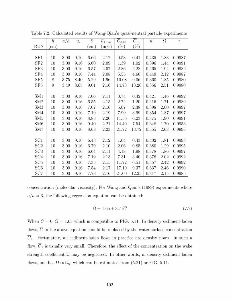
Table 7.2: Calculated results of Wang-Qians quasi-neutral particle experiments
h a/h u∗ δ u1max C0.05 Cm κ Ω rRUN (cm) (cm) (m/s) (%) (%)
SF1 10 3.00 9.16 6.66 2.12 0.53 0.41 0.435 1.83 0.9987SF2 10 3.00 9.16 6.60 2.09 1.39 1.02 0.396 1.44 0.9991SF3 10 3.00 9.16 6.57 2.07 2.86 2.28 0.465 1.94 0.9982SF4 10 3.00 9.16 7.44 2.08 5.55 4.60 0.449 2.12 0.9987SF5 8 3.75 8.40 5.29 1.96 10.08 9.06 0.360 1.85 0.9980SF6 9 3.49 8.65 9.01 2.16 14.73 13.26 0.356 2.51 0.9980
SM1 10 3.00 9.16 7.06 2.11 0.74 0.42 0.421 1.46 0.9992SM2 10 3.00 9.16 6.55 2.15 2.74 1.20 0.416 1.71 0.9989SM3 10 3.00 9.16 7.07 2.16 5.07 2.38 0.398 2.00 0.9997SM4 10 3.00 9.16 7.19 2.19 7.99 3.99 0.354 1.87 0.9997SM5 10 3.00 9.16 8.83 2.20 11.56 6.23 0.375 1.90 0.9991SM6 10 3.00 9.16 9.40 2.21 14.40 7.54 0.348 1.70 0.9953SM7 10 3.00 9.16 8.68 2.23 21.72 13.72 0.355 2.68 0.9995
SC1 10 3.00 9.16 6.43 2.12 1.04 0.43 0.402 1.81 0.9993SC2 10 3.00 9.16 6.79 2.10 2.06 0.85 0.380 1.29 0.9995SC3 10 3.00 9.16 6.64 2.11 4.18 1.98 0.378 1.86 0.9997SC4 10 3.00 9.16 7.19 2.13 7.31 3.40 0.378 2.02 0.9992SC5 10 3.00 9.16 7.35 2.15 11.72 6.51 0.357 2.42 0.9992SC6 10 3.00 9.16 7.54 2.17 17.10 9.37 0.337 2.46 0.9990SC7 10 3.00 9.16 7.73 2.16 21.00 12.25 0.317 2.15 0.9985
concentration (molecular viscosity). For Wang and Qians (1989) experiments where
a/h ≈ 3, the following regression equation can be obtained:
Ω = 1.65 + 3.71C (7.7)
When C = 0, Ω = 1.65 which is compatible to FIG. 5.11. In density sediment-laden
ßows, C in the above equation should be replaced by the water surface concentration
C1. Fortunately, all sediment-laden ßows in practice are density ßows. In such a
ßow, C1 is usually very small. Therefore, the effect of the concentration on the wake
strength coefficient Ω may be neglected. In other words, in density sediment-laden
ßows, one has Ω ≈ Ω0, which can be estimated from (5.21) or FIG. 5.11.
102
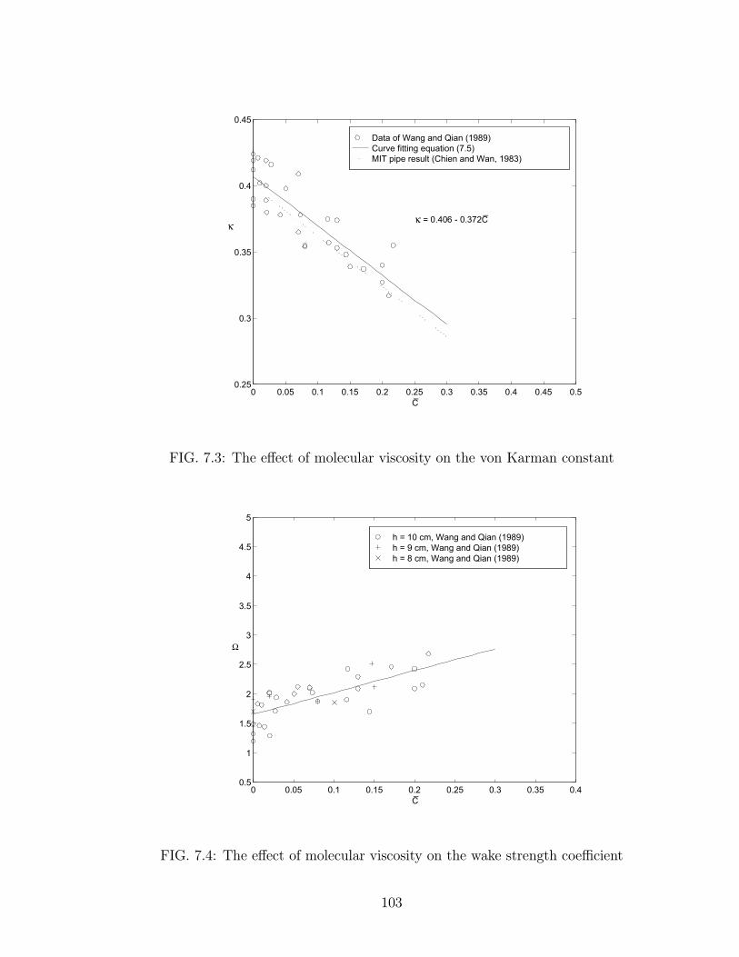
Data of Wang and Qian (1989) Curve fitting equation (7.5) MIT pipe result (Chien and Wan, 1983)
0 0.05 0.1 0.15 0.2 0.25 0.3 0.35 0.4 0.45 0.50.25
0.3
0.35
0.4
0.45
κ = 0.406 - 0.372C
C
κ
FIG. 7.3: The effect of molecular viscosity on the von Karman constant
h = 10 cm, Wang and Qian (1989)h = 9 cm, Wang and Qian (1989) h = 8 cm, Wang and Qian (1989)
0 0.05 0.1 0.15 0.2 0.25 0.3 0.35 0.40.5
1
1.5
2
2.5
3
3.5
4
4.5
5
C
Ω
FIG. 7.4: The effect of molecular viscosity on the wake strength coefficient
103
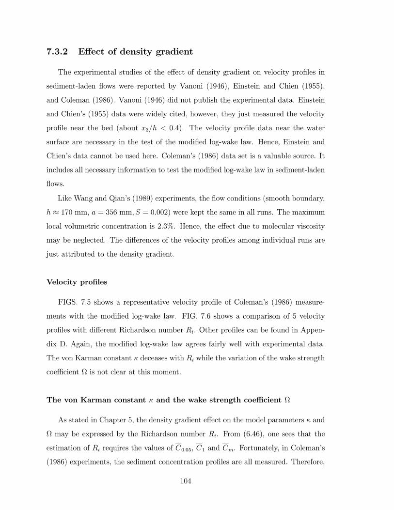
7.3.2 Effect of density gradient
The experimental studies of the effect of density gradient on velocity proÞles in
sediment-laden ßows were reported by Vanoni (1946), Einstein and Chien (1955),
and Coleman (1986). Vanoni (1946) did not publish the experimental data. Einstein
and Chiens (1955) data were widely cited, however, they just measured the velocity
proÞle near the bed (about x3/h < 0.4). The velocity proÞle data near the water
surface are necessary in the test of the modiÞed log-wake law. Hence, Einstein and
Chiens data cannot be used here. Colemans (1986) data set is a valuable source. It
includes all necessary information to test the modiÞed log-wake law in sediment-laden
ßows.
Like Wang and Qians (1989) experiments, the ßow conditions (smooth boundary,
h ≈ 170 mm, a = 356 mm, S = 0.002) were kept the same in all runs. The maximumlocal volumetric concentration is 2.3%. Hence, the effect due to molecular viscosity
may be neglected. The differences of the velocity proÞles among individual runs are
just attributed to the density gradient.
Velocity proÞles
FIGS. 7.5 shows a representative velocity proÞle of Colemans (1986) measure-
ments with the modiÞed log-wake law. FIG. 7.6 shows a comparison of 5 velocity
proÞles with different Richardson number Ri. Other proÞles can be found in Appen-
dix D. Again, the modiÞed log-wake law agrees fairly well with experimental data.
The von Karman constant κ deceases with Ri while the variation of the wake strength
coefficient Ω is not clear at this moment.
The von Karman constant κ and the wake strength coefficient Ω
As stated in Chapter 5, the density gradient effect on the model parameters κ and
Ω may be expressed by the Richardson number Ri. From (6.46), one sees that the
estimation of Ri requires the values of C0.05, C1 and Cm. Fortunately, in Colemans
(1986) experiments, the sediment concentration proÞles are all measured. Therefore,
104
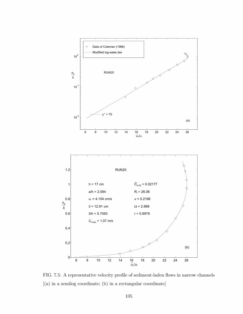
Data of Coleman (1986)
Modified log-wake law
6 8 10 12 14 16 18 20 22 24 26
10-2
10-1
100
u−1/u*
x3
δ___ RUN20
(a)
y+ = 70
6 8 10 12 14 16 18 20 22 24 260
0.2
0.4
0.6
0.8
1
1.2
u−1/u*
x3
δ___
RUN20
h = 17 cm
a/h = 2.094
u* = 4.104 cm/s
δ = 12.91 cm
δ/h = 0.7593
u1max = 1.07 m/s
C0.05 = 0.02177
Ri = 26.06
κ = 0.2166
Ω = 2.888
r = 0.9979
(b)
FIG. 7.5: A representative velocity proÞle of sediment-laden ßows in narrow channels
[(a) in a semilog coordinate; (b) in a rectangular coordinate]
105
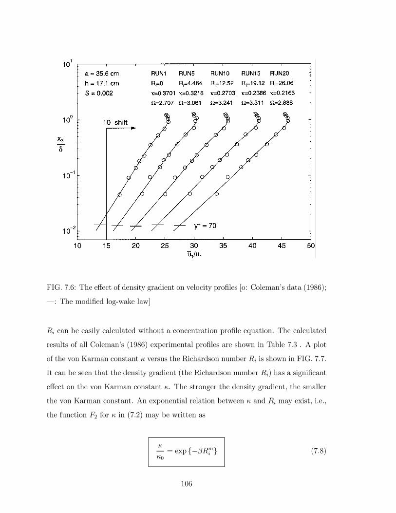
FIG. 7.6: The effect of density gradient on velocity proÞles [o: Colemans data (1986);
: The modiÞed log-wake law]
Ri can be easily calculated without a concentration proÞle equation. The calculated
results of all Colemans (1986) experimental proÞles are shown in Table 7.3 . A plot
of the von Karman constant κ versus the Richardson number Ri is shown in FIG. 7.7.
It can be seen that the density gradient (the Richardson number Ri) has a signiÞcant
effect on the von Karman constant κ. The stronger the density gradient, the smaller
the von Karman constant. An exponential relation between κ and Ri may exist, i.e.,
the function F2 for κ in (7.2) may be written as
κ
κ0= exp −βRmi (7.8)
106
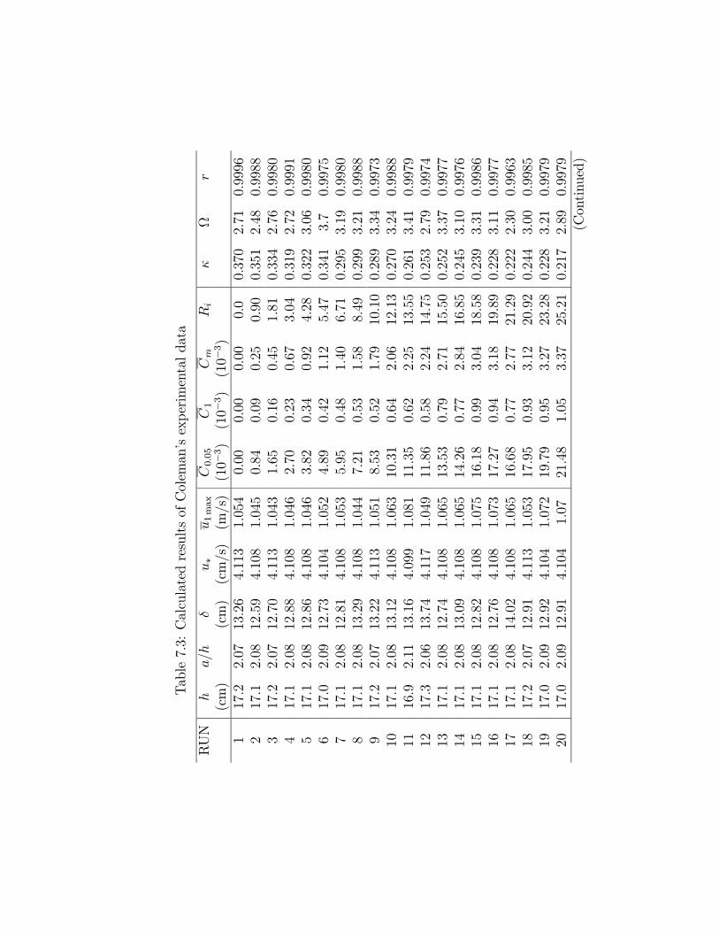
Table7.3:CalculatedresultsofColeman’sexperimentaldata
RUN
ha/h
δu∗
u1max
C0.05
C1
Cm
Ri
κΩ
r(cm)
(cm)(cm/s)(m/s)(10−
3)(10−
3)(10−
3)
117.2
2.07
13.26
4.113
1.054
0.00
0.00
0.00
0.0
0.3702.71
0.9996
217.1
2.08
12.59
4.108
1.045
0.84
0.09
0.25
0.90
0.3512.48
0.9988
317.2
2.07
12.70
4.113
1.043
1.65
0.16
0.45
1.81
0.3342.76
0.9980
417.1
2.08
12.88
4.108
1.046
2.70
0.23
0.67
3.04
0.3192.72
0.9991
517.1
2.08
12.86
4.108
1.046
3.82
0.34
0.92
4.28
0.3223.06
0.9980
617.0
2.09
12.73
4.104
1.052
4.89
0.42
1.12
5.47
0.341
3.7
0.9975
717.1
2.08
12.81
4.108
1.053
5.95
0.48
1.40
6.71
0.2953.19
0.9980
817.1
2.08
13.29
4.108
1.044
7.21
0.53
1.58
8.49
0.2993.21
0.9988
917.2
2.07
13.22
4.113
1.051
8.53
0.52
1.79
10.100.2893.34
0.9973
1017.1
2.08
13.12
4.108
1.063
10.31
0.64
2.06
12.130.2703.24
0.9988
1116.9
2.11
13.16
4.099
1.081
11.35
0.62
2.25
13.550.2613.41
0.9979
1217.3
2.06
13.74
4.117
1.049
11.86
0.58
2.24
14.750.2532.79
0.9974
1317.1
2.08
12.74
4.108
1.065
13.53
0.79
2.71
15.500.2523.37
0.9977
1417.1
2.08
13.09
4.108
1.065
14.26
0.77
2.84
16.850.2453.10
0.9976
1517.1
2.08
12.82
4.108
1.075
16.18
0.99
3.04
18.580.2393.31
0.9986
1617.1
2.08
12.76
4.108
1.073
17.27
0.94
3.18
19.890.2283.11
0.9977
1717.1
2.08
14.02
4.108
1.065
16.68
0.77
2.77
21.290.2222.30
0.9963
1817.2
2.07
12.91
4.113
1.053
17.95
0.93
3.12
20.920.2443.00
0.9985
1917.0
2.09
12.92
4.104
1.072
19.79
0.95
3.27
23.280.2283.21
0.9979
2017.0
2.09
12.91
4.104
1.07
21.48
1.05
3.37
25.210.2172.89
0.9979
(Continued)
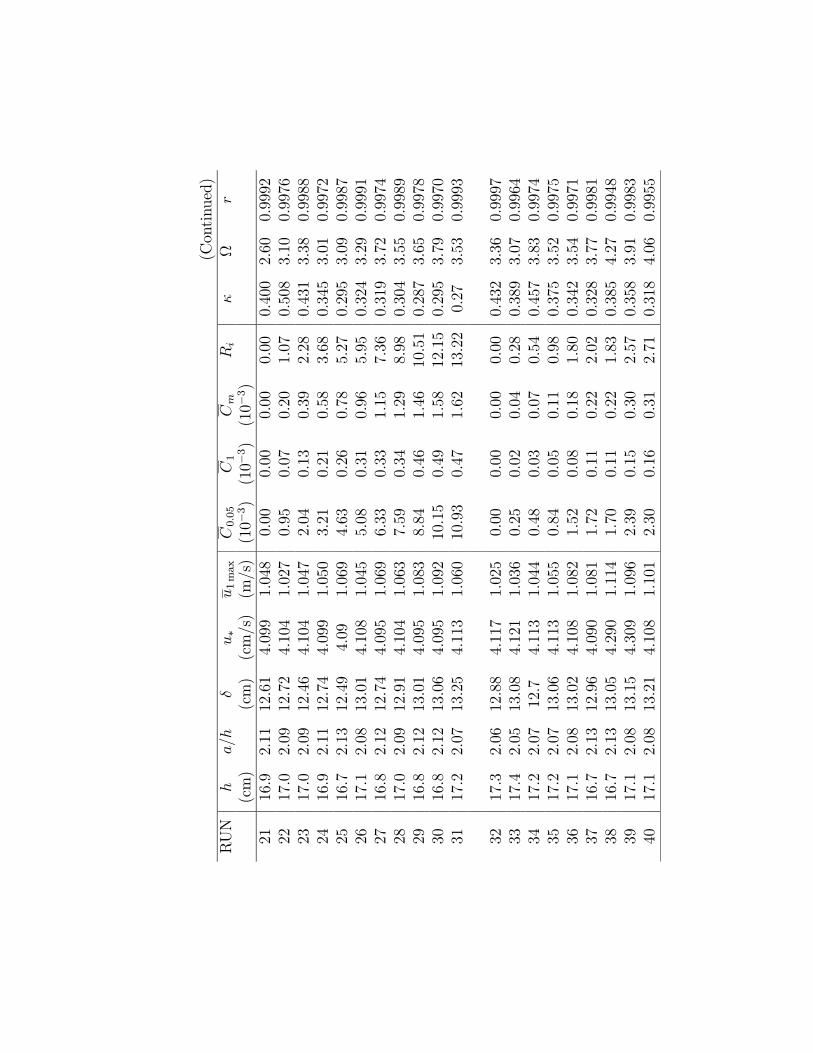
(Continued)
RUN
ha/h
δu∗
u1max
C0.05
C1
Cm
Ri
κΩ
r(cm)
(cm)(cm/s)(m/s)(10−
3)(10−
3)(10−
3)
2116.9
2.11
12.61
4.099
1.048
0.00
0.00
0.00
0.00
0.4002.60
0.9992
2217.0
2.09
12.72
4.104
1.027
0.95
0.07
0.20
1.07
0.5083.10
0.9976
2317.0
2.09
12.46
4.104
1.047
2.04
0.13
0.39
2.28
0.4313.38
0.9988
2416.9
2.11
12.74
4.099
1.050
3.21
0.21
0.58
3.68
0.3453.01
0.9972
2516.7
2.13
12.49
4.09
1.069
4.63
0.26
0.78
5.27
0.2953.09
0.9987
2617.1
2.08
13.01
4.108
1.045
5.08
0.31
0.96
5.95
0.3243.29
0.9991
2716.8
2.12
12.74
4.095
1.069
6.33
0.33
1.15
7.36
0.3193.72
0.9974
2817.0
2.09
12.91
4.104
1.063
7.59
0.34
1.29
8.98
0.3043.55
0.9989
2916.8
2.12
13.01
4.095
1.083
8.84
0.46
1.46
10.510.2873.65
0.9978
3016.8
2.12
13.06
4.095
1.092
10.15
0.49
1.58
12.150.2953.79
0.9970
3117.2
2.07
13.25
4.113
1.060
10.93
0.47
1.62
13.22
0.27
3.53
0.9993
3217.3
2.06
12.88
4.117
1.025
0.00
0.00
0.00
0.00
0.4323.36
0.9997
3317.4
2.05
13.08
4.121
1.036
0.25
0.02
0.04
0.28
0.3893.07
0.9964
3417.2
2.07
12.7
4.113
1.044
0.48
0.03
0.07
0.54
0.4573.83
0.9974
3517.2
2.07
13.06
4.113
1.055
0.84
0.05
0.11
0.98
0.3753.52
0.9975
3617.1
2.08
13.02
4.108
1.082
1.52
0.08
0.18
1.80
0.3423.54
0.9971
3716.7
2.13
12.96
4.090
1.081
1.72
0.11
0.22
2.02
0.3283.77
0.9981
3816.7
2.13
13.05
4.290
1.114
1.70
0.11
0.22
1.83
0.3854.27
0.9948
3917.1
2.08
13.15
4.309
1.096
2.39
0.15
0.30
2.57
0.3583.91
0.9983
4017.1
2.08
13.21
4.108
1.101
2.30
0.16
0.31
2.71
0.3184.06
0.9955
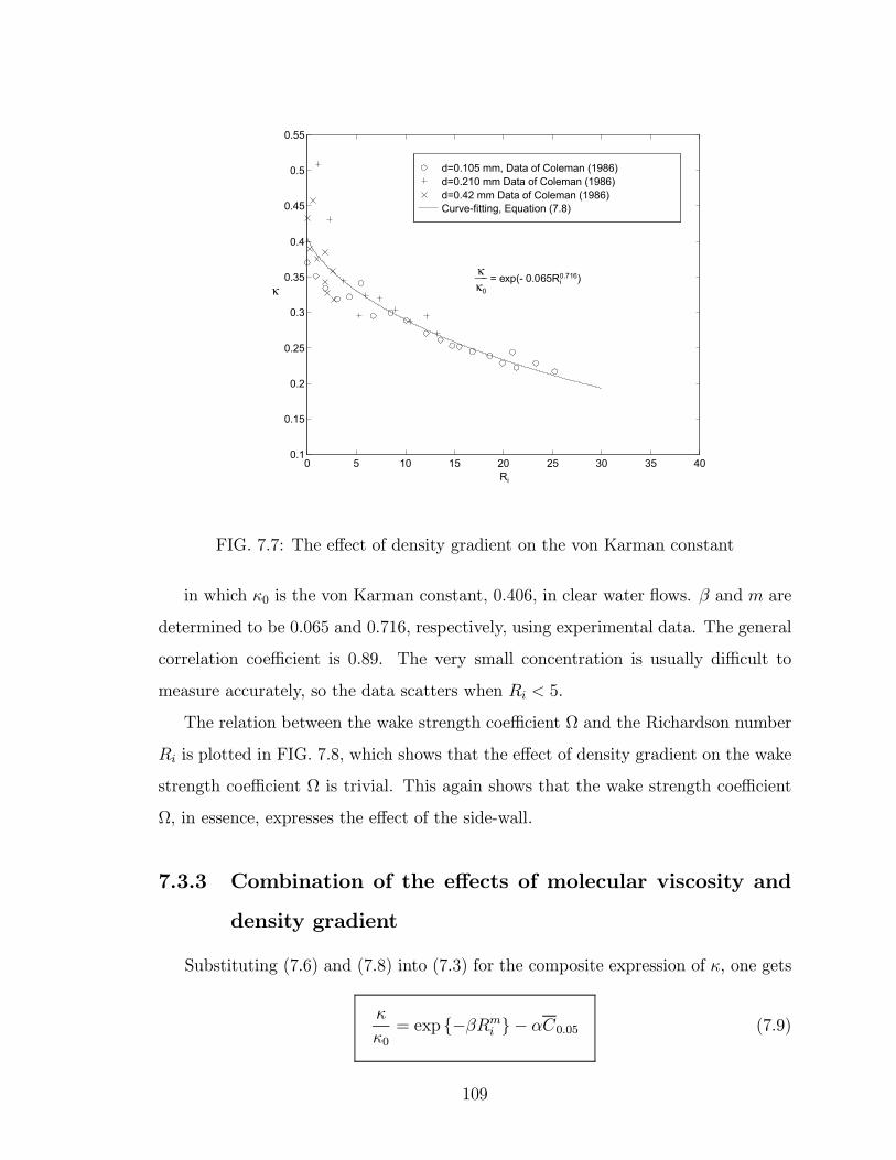
d=0.105 mm, Data of Coleman (1986)d=0.210 mm Data of Coleman (1986) d=0.42 mm Data of Coleman (1986) Curve-fitting, Equation (7.8)
0 5 10 15 20 25 30 35 400.1
0.15
0.2
0.25
0.3
0.35
0.4
0.45
0.5
0.55
Ri
κκκ0
___ = exp(- 0.065Ri0.716)
FIG. 7.7: The effect of density gradient on the von Karman constant
in which κ0 is the von Karman constant, 0.406, in clear water ßows. β and m are
determined to be 0.065 and 0.716, respectively, using experimental data. The general
correlation coefficient is 0.89. The very small concentration is usually difficult to
measure accurately, so the data scatters when Ri < 5.
The relation between the wake strength coefficient Ω and the Richardson number
Ri is plotted in FIG. 7.8, which shows that the effect of density gradient on the wake
strength coefficient Ω is trivial. This again shows that the wake strength coefficient
Ω, in essence, expresses the effect of the side-wall.
7.3.3 Combination of the effects of molecular viscosity and
density gradient
Substituting (7.6) and (7.8) into (7.3) for the composite expression of κ, one gets
κ
κ0= exp −βRmi − αC0.05 (7.9)
109
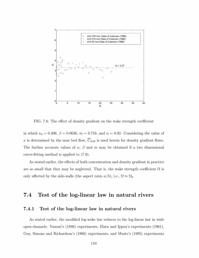
d=0.105 mm, Data of Coleman (1986)d=0.210 mm Data of Coleman (1986) d=0.42 mm Data of Coleman (1986)
0 5 10 15 20 25 30 35 400
1
2
3
4
5
6
7
Ri
Ω Ω = 3.27
FIG. 7.8: The effect of density gradient on the wake strength coefficient
in which κ0 = 0.406, β = 0.0636, m = 0.716, and α = 0.92. Considering the value of
κ is determined by the near bed ßow, C0.05 is used herein for density gradient ßows.
The further accurate values of α, β and m may be obtained if a two dimensional
curve-Þtting method is applied to (7.9).
As stated earlier, the effects of both concentration and density gradient in practice
are so small that they may be neglected. That is, the wake strength coefficient Ω is
only affected by the side-walls (the aspect ratio a/h), i.e., Ω ≈ Ω0.
7.4 Test of the log-linear law in natural rivers
7.4.1 Test of the log-linear law in natural rivers
As stated earlier, the modiÞed log-wake law reduces to the log-linear law in wide
open-channels. Vanonis (1946) experiments, Elata and Ippens experiments (1961),
Guy, Simons and Richardsons (1966) experiments, and Mustes (1995) experiments
110
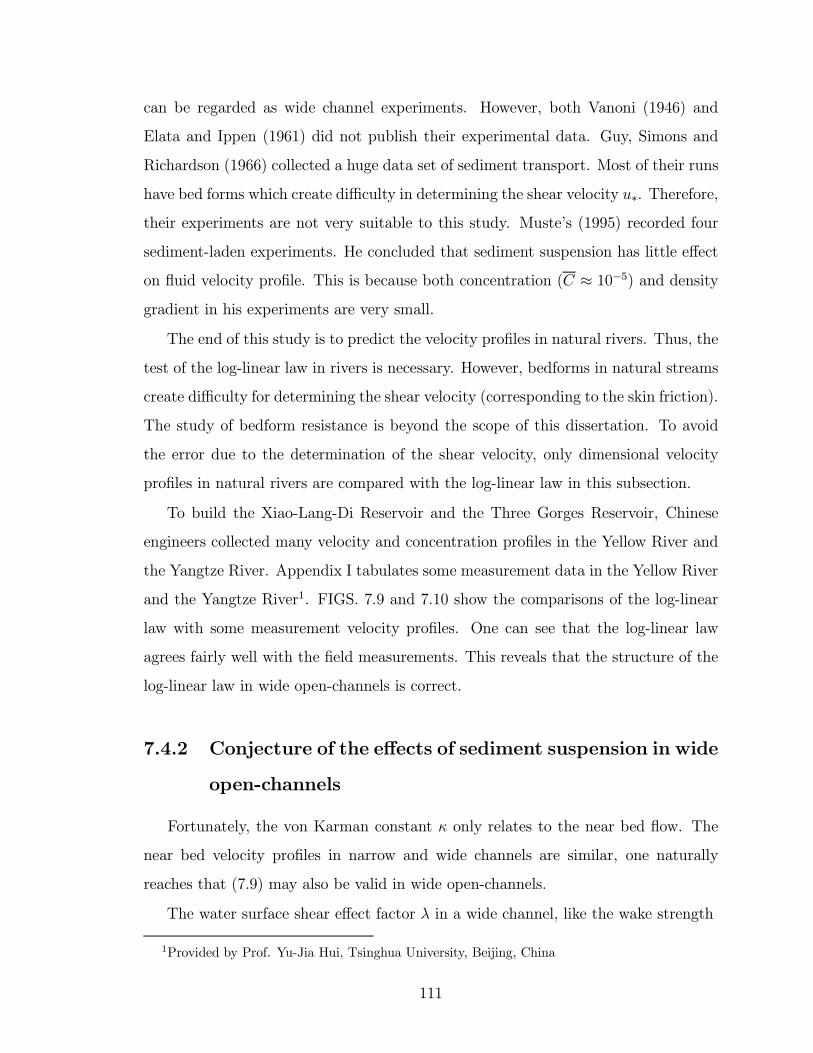
can be regarded as wide channel experiments. However, both Vanoni (1946) and
Elata and Ippen (1961) did not publish their experimental data. Guy, Simons and
Richardson (1966) collected a huge data set of sediment transport. Most of their runs
have bed forms which create difficulty in determining the shear velocity u∗. Therefore,
their experiments are not very suitable to this study. Mustes (1995) recorded four
sediment-laden experiments. He concluded that sediment suspension has little effect
on ßuid velocity proÞle. This is because both concentration (C ≈ 10−5) and densitygradient in his experiments are very small.
The end of this study is to predict the velocity proÞles in natural rivers. Thus, the
test of the log-linear law in rivers is necessary. However, bedforms in natural streams
create difficulty for determining the shear velocity (corresponding to the skin friction).
The study of bedform resistance is beyond the scope of this dissertation. To avoid
the error due to the determination of the shear velocity, only dimensional velocity
proÞles in natural rivers are compared with the log-linear law in this subsection.
To build the Xiao-Lang-Di Reservoir and the Three Gorges Reservoir, Chinese
engineers collected many velocity and concentration proÞles in the Yellow River and
the Yangtze River. Appendix I tabulates some measurement data in the Yellow River
and the Yangtze River1. FIGS. 7.9 and 7.10 show the comparisons of the log-linear
law with some measurement velocity proÞles. One can see that the log-linear law
agrees fairly well with the Þeld measurements. This reveals that the structure of the
log-linear law in wide open-channels is correct.
7.4.2 Conjecture of the effects of sediment suspension in wide
open-channels
Fortunately, the von Karman constant κ only relates to the near bed ßow. The
near bed velocity proÞles in narrow and wide channels are similar, one naturally
reaches that (7.9) may also be valid in wide open-channels.
The water surface shear effect factor λ in a wide channel, like the wake strength
1Provided by Prof. Yu-Jia Hui, Tsinghua University, Beijing, China
111
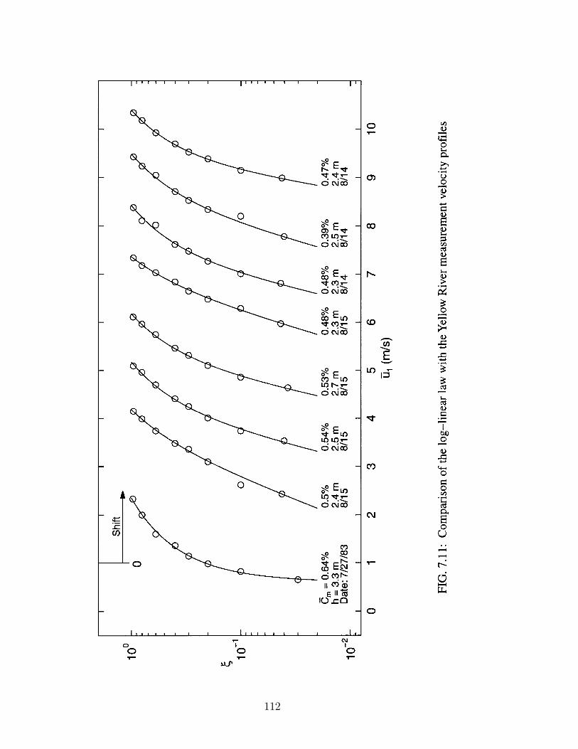
112
113
coefficient Ω in narrow channels, only relates to the near surface ßow. Since both
concentration and density gradient at the water surface are usually very small, their
effects on λ may be neglected. Thus, (5.33), from clear water, may also be valid in
sediment-laden ßows.
7.5 Summary
In this chapter, the modiÞed log-wake law Þrst compares with neutral particle-
laden experiments in narrow channels. It shows that the von Karman constant κ de-
creases with volumetric sediment concentration and can be estimated from (7.6). This
is because sediment concentration increases molecular viscosity and then increases
energy dissipation. The wake strength coefficient Ω slightly increases with sediment
concentration, but its effect may, in practice, be neglected in density sediment-laden
ßows. Note that a neutral particle-laden ßow belongs to a two-phase ßow, which is
different from a one-phase thick ßuid. Given the same boundary condition, a two-
phase ßow dissipates more energy than a one-phase thick ßow. This is because in a
two-phase (liquid + solid particles) ßow, solid particles increase the effective surface
between ßuid and solid boundaries.
The modiÞed log-wake is then tested with density sediment-laden experiments in
narrow channels. It shows that the von Karman constant κ also decreases with the
Richardson number Ri (density gradient) and can be estimated from (7.8). Unlike κ,
the wake strength coefficient Ω has little to do with the Richardson number Ri. It
may still be estimated from (5.21).
The log-linear law, which is the reduction of the log-wake law in wide channels,
compares quite well with measurement velocity proÞles in the Yellow River and the
Yangtze River. It is conjectured that like the wake strength coefficient Ω, sediment
suspension may have little effect on the water surface shear correction factor λ.
The combination of the effects of concentration and density gradient on the von
Karman constant κ may be expressed by (7.9). It may be valid in both narrow and
wide channels.
114
Chapter 8
APPLICATIONS OF THE
MODIFIED LOG-WAKE LAW
8.1 Applications of the modiÞed log-wake law in
pipes
8.1.1 Relation between the maximum velocity u1max and the
average velocity U
Neglecting the viscous sublayer and the buffer layer and integrating (5.1) over the
cross-sectional area, one obtains that
u1max − Uu∗
= 2
Z 1
0
·− 1κ0ln ξ + Ω0 cos
2 πξ
2− 1− ξ
κ0
¸(1− ξ) dξ
= − 2κ0
Z 1
0
(1− ξ) ln ξ + 2Ω0Z 1
0
(1− ξ) cos2 πξ2dξ − 2
κ0
Z 1
0
(1− ξ)2dξ
Since Z 1
0
(1− ξ) ln ξ =
Z 1
0
ln ξdξ −Z 1
0
ξ ln ξdξ
= −1−·ξ2
2ln ξ − ξ
2
4
¸10
= −1 + 14= −3
4
115
Z 1
0
(1− ξ) cos2 πξ2dξ
=
Z 1
0
cos2πξ
2dξ −
Z 1
0
ξ cos2πξ
2dξ
=2
π
Z π/2
0
cos2 ξdξ −Z 1
0
1 + cos πξ
2ξdξ
=1
2−µ1
4+1
2
Z 1
0
ξ cosπξdξ
¶=
1
4− 12
µ1
π2cosπξ +
ξ
πsin πξ
¶10
=1
4+1
π2
and Z 1
0
(1− ξ)2dξ = 1
3
one has
u1max − Uu∗
= − 2κ0
·−34
¸+ 2Ω0
·1
4+1
π2
¸− 2
κ0
µ1
3
¶=
5
6κ0+
µ1
2+2
π2
¶Ω0
Taking κ0 = 0.406 and Ω0 = 3.2, one obtains
u1max − Uu∗
= 4.3 (8.1)
8.1.2 Position of the average velocity U
Equating the right-hand side of (5.1) to the right-hand side of (8.1) and solving
the resultant equation, one obtains the position of the average velocity U , which is
ξ = 0.25 (8.2)
This equation can be used to measure the pipe average velocity at one point.
8.1.3 Procedures for applying the modiÞed log-wake law
Provided that the pipe diameter d, the shear velocity u∗ (or the pipe length L and
the pressure drop ∆p), one can calculate the pipe velocity proÞle as follows:
116
Step 1: Estimate the friction factor f , which is deÞned as f = 8 (u∗/U)2, and
the average velocity U . The study of the friction factor is beyond this dissertation.
Prandtls classical equation (Schlichting, 1979, p.611, p.624) or Zagarolas (1996)
resistance formula may be used.
Prandtls formula (Schlichting, 1979, p.611, p.624):
1√f= 2 log
³Repf´− 0.8 (hydraulically smooth) (8.3)
in which Re= Ud/ν. The above equation is valid up to Re= 3.4× 10⁶.
f =1³
2 log Rks+ 1.74
´2 (completely rough) (8.4)
in which R is the pipe radius; and ks is roughness.
Zagarolas (1996, p.204) formula (hydraulically smooth):
1√f= 1.872 log
³Repf´− 0.2555− 228¡
Re√f¢0.89 (8.5)
which is valid for Re= 3.1× 10⁴ − 3.5× 10⁷.Step 2: With the average velocity U available, the maximum velocity u1max can
be estimated using (8.1).
Step 3: Given the maximum velocity u1max, the shear velocity u∗, κ0 = 0.406, and
Ω0 = 3.2, the velocity proÞle can be estimated using (5.1), i.e.
u1max − u1u∗
= − 1κ0ln ξ + Ω0 cos
2 πξ
2− 1− ξ
κ0
8.2 Applications of the modiÞed log-wake law in
open-channels
The ßow in a narrow open-channel is three-dimensional and much more compli-
cated than that in a wide open-channel. The velocity proÞle over the whole cross-
section in a narrow channel is not studied in this dissertation. So, a full application
of the modiÞed log-wake law in narrow channels cannot be recommended at this mo-
ment. However, the log-linear law, which is the reduction of the modiÞed log-wake
law in wide channels, has been ready to apply in wide open-channel ßows.
117
8.2.1 Magnitude of the linear term in the log-linear law
From (5.23), the linear term in the log-linear law is
−"1
κ− λ0
µVwind − u1max
u∗
¶2#(1− ξ)
in which κ is the von Karman constant in sediment-laden ßows and varies between
0.2 and 0.406, λ0 ≈ 0.0065. Usually, u1max/u∗ = 10− 30. If Vwind = 0, one has
−5 < −"1
κ− λ0
µVwind − u1max
u∗
¶2#< 4 (8.6)
One can see that the coefficient of the linear term may be positive and may be
negative. In some cases, the coefficient may be close to zero, the linear term may be
neglected and the classical log law is restored. However, this cannot be generalized.
In particular, the linear term cannot be neglected in a sediment-laden ßow. This can
be easily seen from FIGS. 7.9 and 7.10, where the velocity proÞles are not straight
lines in a semilog coordinate system.
8.2.2 Relation between the maximum velocity u1max and the
average velocity U
For a wide open-channel (2D), neglecting the viscous sublayer and the buffer layer
and integrating the log-linear law (5.23) over the entire ßow depth, one has
u1max − Uu∗
=
Z 1
0
(−1κln ξ −
"1
κ− λ0
µVwind − u1max
u∗
¶2#(1− ξ)
)dξ
= −1κ
Z 1
0
ln ξdξ −"1
κ− λ0
µVwind − u1max
u∗
¶2#Z 1
0
(1− ξ)dξ
=1
κ− 12
"1
κ− λ0
µVwind − u1max
u∗
¶2#
=1
2κ+λ02
µVwind − u1max
u∗
¶2(8.7)
i.e.λ02
µVwind − u1max
u∗
¶2− u1max − U
u∗+1
2κ= 0 (8.8)
118
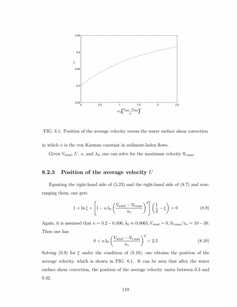
0 0.5 1 1.5 2 2.50.25
0.3
0.35
0.4
0.45
κλ0(Vwind − u1max
u*
___________)2
ξ
FIG. 8.1: Position of the average velocity versus the water surface shear correction
in which κ is the von Karman constant in sediment-laden ßows.
Given Vwind, U , κ, and λ0, one can solve for the maximum velocity u1max.
8.2.3 Position of the average velocity U
Equating the right-hand side of (5.23) and the right-hand side of (8.7) and rear-
ranging them, one gets
1 + ln ξ +
"1− κλ0
µVwind − u1max
u∗
¶2#µ1
2− ξ¶= 0 (8.9)
Again, it is assumed that κ = 0.2−0.406,λ0 ≈ 0.0065, Vwind = 0, u1max/u∗ = 10−30.Then one has
0 < κλ0
µVwind − u1max
u∗
¶2< 2.5 (8.10)
Solving (8.9) for ξ under the condition of (8.10), one obtains the position of the
average velocity, which is shown in FIG. 8.1. It can be seen that after the water
surface shear correction, the position of the average velocity varies between 0.3 and
0.42.
119
8.2.4 Procedures for applying the log-linear law
Assume a uniform ßow in a wide channel with a plane bed. Provided that the
ßow depth h, the bed slope S, the sediment size ds, and the volumetric sediment
concentration C0.05, one may estimate the velocity proÞle in the following way:
Step 1: Estimate the shear velocity u∗, i.e., u∗ =√ghS, where g is the gravita-
tional acceleration. Note that for bedform channels, the skin shear velocity u0∗ should
be used.
Step 2: Estimate the average velocity U . The classical resistance equation by
Keulegan (Chien and Wan, 1983, p.205) may be used, i.e.
U
u∗= 5.75 log
µhu∗ν
¶+ 3.25 (hydraulically smooth) (8.11)
U
u∗= 5.75 log
µh
ks
¶+ 6.25 (completely rough) (8.12)
in which ν is the water kinematic viscosity; and the roughness ks is usually taken as
(2− 7)d50 (Chien and Wan, 1983, p.206; Julien, 1995, p.96). For sand bed channels,ks = 2.5d50 may be used.
Step 3: Estimate the Richardson number from (6.46), i.e.
Ri =gδ
u2∗
ρs − ρ0ρ0
C0.05 − C11 +
ρs − ρ0ρ0
Cm
in which δ = h for wide open-channels. For density sediment-laden ßows, usually
C1 << C0.05, and Cm << 1. Then the above expression reduces to
Ri =gδ
u2∗
ρs − ρ0ρ0
C0.05 (8.13)
Step 4: Estimate the von Karman constant κ from (7.9), i.e.
κ
κ0= exp−βRmi − αC0.05
in which κ0 = 0.406, β = 0.0636,m = 0.716, and α = 0.92.
Step 5: Assume λ0 = 0.0065 for sand channels or calculate λ0 from (5.33) for
gravel channels. With κ, u∗ and U , estimate the maximum velocity u1max from (8.8).
120
Step 6: Estimate the velocity proÞle with the log-linear law, i.e.
u1max − u1u∗
= −1κln ξ −
"1
κ− λ0
µVwind − u1max
u∗
¶2#(1− ξ)
in which Vwind may be assumed to be zero in laboratory or measured in Þeld cases.
121
Chapter 9
SUMMARY AND
CONCLUSIONS
9.1 Summary
Turbulent velocity proÞles in pipes and open-channels with clear water and sediment-
laden ßows are investigated. A new similarity analysis method, the four-step similarity
analysis method, is Þrst presented, which includes dimensional analysis, intermediate
asymptotics, wake correction, and boundary correction. Based on the four-step simi-
larity analysis method, a clear water velocity proÞle model, the modiÞed log-wake law,
is proposed. The modiÞed log-wake law consists of three components: a log term, a
wake term, and a linear term. Physically, the log term expresses the inertia effect; the
wake term expresses the large-scale turbulent mixing; and the linear term expresses
the boundary condition effect. In open-channels, the wake term reßects the side-wall
effect. A theoretical analysis and a magnitude order analysis show that the modiÞed
log-wake law is also valid in sediment-laden ßows. In particular, the modiÞed log-
wake law considers the derivative boundary condition at the boundary layer margin,
which is not satisÞed in previous studies.
The modiÞed log-wake law has compared quite well with experiments in pipes,
narrow open-channels and wide open-channels, including both clear water ßows and
sediment-laden ßows.
122
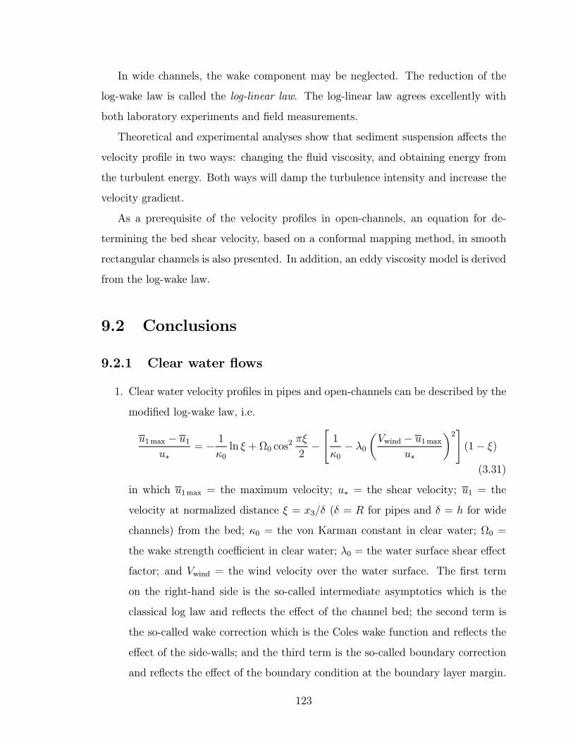
In wide channels, the wake component may be neglected. The reduction of the
log-wake law is called the log-linear law. The log-linear law agrees excellently with
both laboratory experiments and Þeld measurements.
Theoretical and experimental analyses show that sediment suspension affects the
velocity proÞle in two ways: changing the ßuid viscosity, and obtaining energy from
the turbulent energy. Both ways will damp the turbulence intensity and increase the
velocity gradient.
As a prerequisite of the velocity proÞles in open-channels, an equation for de-
termining the bed shear velocity, based on a conformal mapping method, in smooth
rectangular channels is also presented. In addition, an eddy viscosity model is derived
from the log-wake law.
9.2 Conclusions
9.2.1 Clear water ßows
1. Clear water velocity proÞles in pipes and open-channels can be described by the
modiÞed log-wake law, i.e.
u1max − u1u∗
= − 1κ0ln ξ + Ω0 cos
2 πξ
2−"1
κ0− λ0
µVwind − u1max
u∗
¶2#(1− ξ)(3.31)
in which u1max = the maximum velocity; u∗ = the shear velocity; u1 = the
velocity at normalized distance ξ = x3/δ (δ = R for pipes and δ = h for wide
channels) from the bed; κ0 = the von Karman constant in clear water; Ω0 =
the wake strength coefficient in clear water; λ0 = the water surface shear effect
factor; and Vwind = the wind velocity over the water surface. The Þrst term
on the right-hand side is the so-called intermediate asymptotics which is the
classical log law and reßects the effect of the channel bed; the second term is
the so-called wake correction which is the Coles wake function and reßects the
effect of the side-walls; and the third term is the so-called boundary correction
and reßects the effect of the boundary condition at the boundary layer margin.
123
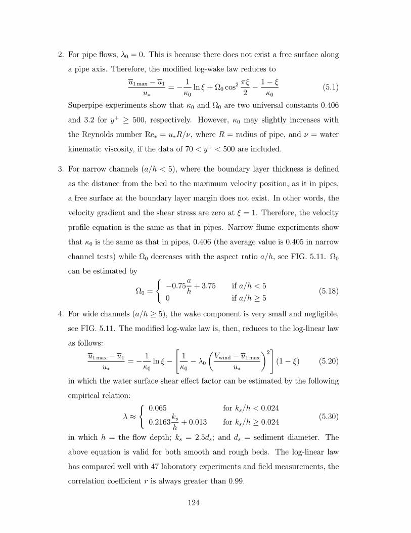
2. For pipe ßows, λ0 = 0. This is because there does not exist a free surface along
a pipe axis. Therefore, the modiÞed log-wake law reduces to
u1max − u1u∗
= − 1κ0ln ξ + Ω0 cos
2 πξ
2− 1− ξ
κ0(5.1)
Superpipe experiments show that κ0 and Ω0 are two universal constants 0.406
and 3.2 for y+ ≥ 500, respectively. However, κ0 may slightly increases with
the Reynolds number Re∗ = u∗R/ν, where R = radius of pipe, and ν = water
kinematic viscosity, if the data of 70 < y+ < 500 are included.
3. For narrow channels (a/h < 5), where the boundary layer thickness is deÞned
as the distance from the bed to the maximum velocity position, as it in pipes,
a free surface at the boundary layer margin does not exist. In other words, the
velocity gradient and the shear stress are zero at ξ = 1. Therefore, the velocity
proÞle equation is the same as that in pipes. Narrow ßume experiments show
that κ0 is the same as that in pipes, 0.406 (the average value is 0.405 in narrow
channel tests) while Ω0 decreases with the aspect ratio a/h, see FIG. 5.11. Ω0
can be estimated by
Ω0 =
(−0.75a
h+ 3.75 if a/h < 5
0 if a/h ≥ 5(5.18)
4. For wide channels (a/h ≥ 5), the wake component is very small and negligible,see FIG. 5.11. The modiÞed log-wake law is, then, reduces to the log-linear law
as follows:
u1max − u1u∗
= − 1κ0ln ξ −
"1
κ0− λ0
µVwind − u1max
u∗
¶2#(1− ξ) (5.20)
in which the water surface shear effect factor can be estimated by the following
empirical relation:
λ ≈(0.065 for ks/h < 0.024
0.2163ksh+ 0.013 for ks/h ≥ 0.024 (5.30)
in which h = the ßow depth; ks = 2.5ds; and ds = sediment diameter. The
above equation is valid for both smooth and rough beds. The log-linear law
has compared well with 47 laboratory experiments and Þeld measurements, the
correlation coefficient r is always greater than 0.99.
124
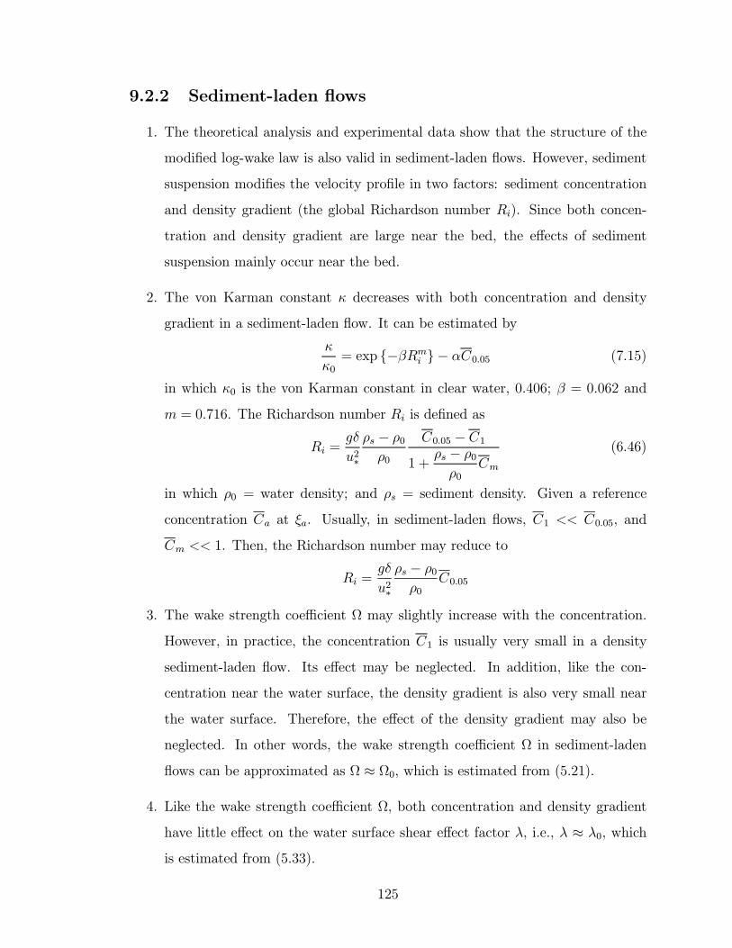
9.2.2 Sediment-laden ßows
1. The theoretical analysis and experimental data show that the structure of the
modiÞed log-wake law is also valid in sediment-laden ßows. However, sediment
suspension modiÞes the velocity proÞle in two factors: sediment concentration
and density gradient (the global Richardson number Ri). Since both concen-
tration and density gradient are large near the bed, the effects of sediment
suspension mainly occur near the bed.
2. The von Karman constant κ decreases with both concentration and density
gradient in a sediment-laden ßow. It can be estimated by
κ
κ0= exp −βRmi − αC0.05 (7.15)
in which κ0 is the von Karman constant in clear water, 0.406; β = 0.062 and
m = 0.716. The Richardson number Ri is deÞned as
Ri =gδ
u2∗
ρs − ρ0ρ0
C0.05 − C11 +
ρs − ρ0ρ0
Cm
(6.46)
in which ρ0 = water density; and ρs = sediment density. Given a reference
concentration Ca at ξa. Usually, in sediment-laden ßows, C1 << C0.05, and
Cm << 1. Then, the Richardson number may reduce to
Ri =gδ
u2∗
ρs − ρ0ρ0
C0.05
3. The wake strength coefficient Ω may slightly increase with the concentration.
However, in practice, the concentration C1 is usually very small in a density
sediment-laden ßow. Its effect may be neglected. In addition, like the con-
centration near the water surface, the density gradient is also very small near
the water surface. Therefore, the effect of the density gradient may also be
neglected. In other words, the wake strength coefficient Ω in sediment-laden
ßows can be approximated as Ω ≈ Ω0, which is estimated from (5.21).
4. Like the wake strength coefficient Ω, both concentration and density gradient
have little effect on the water surface shear effect factor λ, i.e., λ ≈ λ0, whichis estimated from (5.33).
125
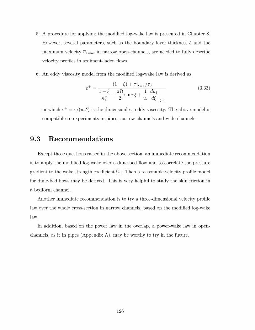
5. A procedure for applying the modiÞed log-wake law is presented in Chapter 8.
However, several parameters, such as the boundary layer thickness δ and the
maximum velocity u1max in narrow open-channels, are needed to fully describe
velocity proÞles in sediment-laden ßows.
6. An eddy viscosity model from the modiÞed log-wake law is derived as
ε+ =(1− ξ) + τ |ξ=1 /τ0
1− ξκξ
+πΩ
2sin πξ +
1
u∗
du1dξ
¯ξ=1
(3.33)
in which ε+ = ε/(u∗δ) is the dimensionless eddy viscosity. The above model is
compatible to experiments in pipes, narrow channels and wide channels.
9.3 Recommendations
Except those questions raised in the above section, an immediate recommendation
is to apply the modiÞed log-wake over a dune-bed ßow and to correlate the pressure
gradient to the wake strength coefficient Ω0. Then a reasonable velocity proÞle model
for dune-bed ßows may be derived. This is very helpful to study the skin friction in
a bedform channel.
Another immediate recommendation is to try a three-dimensional velocity proÞle
law over the whole cross-section in narrow channels, based on the modiÞed log-wake
law.
In addition, based on the power law in the overlap, a power-wake law in open-
channels, as it in pipes (Appendix A), may be worthy to try in the future.
126
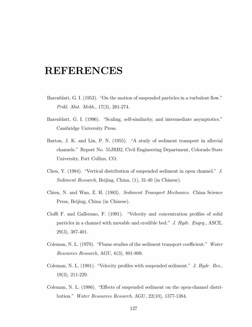
REFERENCES
Barenblatt, G. I. (1953). On the motion of suspended particles in a turbulent ßow.
Prikl. Mat. Mekh., 17(3), 261-274.
Barenblatt, G. I. (1996). Scaling, self-similarity, and intermediate asymptotics.
Cambridge University Press.
Barton, J. K. and Lin, P. N. (1955). A study of sediment transport in alluvial
channels. Report No. 55JRB2, Civil Engineering Department, Colorado State
University, Fort Collins, CO.
Chen, Y. (1984). Vertical distribution of suspended sediment in open channel. J.
Sediment Research, Beijing, China, (1), 31-40 (in Chinese).
Chien, N. and Wan, Z. H. (1983). Sediment Transport Mechanics. China Science
Press, Beijing, China (in Chinese).
Cioffi F. and Gallerano, F. (1991). Velocity and concentration proÞles of solid
particles in a channel with movable and erodible bed. J. Hydr. Engrg., ASCE,
29(3), 387-401.
Coleman, N. L. (1970). Flume studies of the sediment transport coefficient. Water
Resources Research, AGU, 6(3), 801-809.
Coleman, N. L. (1981). Velocity proÞles with suspended sediment. J. Hydr. Res.,
19(3), 211-229.
Coleman, N. L. (1986). Effects of suspended sediment on the open-channel distri-
bution. Water Resources Research, AGU, 22(10), 1377-1384.
127
Coles, D. E. (1956). The law of the wake in the turbulent boundary layer. J.
Fluid Mechanics, 1, 191-226.
Coles, D. (1969). The young persons guide to the data. Proceedings Computation
of Turbulent Boundary Layers 1968 AFOSR-IFP-STANFORD CONFER-
ENCE, 2, 1-19.
Dou, Guoren (1987). Turbulence, Vol. 2, Higher Education Press, Beijing, China
(in Chinese).
Einstein, H. A. and Chien, N. (1955). Effects of heavy sediment concentration near
the bed on velocity and sediment distribution. U. S. Army Corps of Engineers,
Missouri River Division Rep. No. 8.
Elata, C. and Ippen, A. T. (1961). The dynamics of open channel ßow with suspen-
sions of neutrally buoyant particles. Technical Report No. 45, Hydrodynamics
Lab, MIT.
Guy, H. P., Simons, D. B. and Richardson, E. V. (1966). Summary of alluvial
channel data from ßume experiments, 1956-1961. USGS Professional Paper
462-I.
Hinze, J. O. (1975). Turbulence. 2nd Ed., McGraw-Hill, New York.
Hu, C. H. and Hui, Y. J. (1995). Mechanical and Statistical Laws in Open-Channel
Flows. China Science Press, Beijing, China (in Chinese).
Ippen, A. T. (1971). A new look at sedimentation in turbulent streams. J. Boston
Civil Engineers, 58(3), 131-163.
Itakura, T. and Kishi, T. (1980). Open channel ßow with suspended sediments.
J. Hydr. Div., ASCE, 106(8), 1325-1343.
Janin, L. F. (1986). Sediment-laden velocity proÞles developed in a large boundary-
layer wind tunnel.. PhD dissertation, Colorado State University, Fort Collins,
CO.
128
Julien, P. Y. (1995). Erosion and Sedimentation. Cambridge University Press.
Karim, M. F. and Kennedy, J. F. (1987). velocity and sediment-concentration
proÞles in river ßows. J. Hydr. Engrg., ASCE, 113(2), 159-178.
Kereselidze, N. B. and Kutavaia, V. I. (1995). Experimental research on kinematics
of ßows with high suspended solid concentration. J. Hydr. Res., 33(1), 65-75.
Keulegan, G. H. (1938). Laws of turbulent ßow in open channels. J. Research.,
Nat. Bureau of Standards, 21(6), 707-741.
Kironoto, B. A. (1993). Turbulence characteristics of uniform and non-uniform,
rough open-channel ßow. PhD Dissertation, Swiss Federal Institute of Technol-
ogy at Lausanne, Switzerland.
Kironoto, B. A. and Graf, W. H. (1994). Turbulence characteristics in rough uni-
form open-channel ßow. Proc. Instn Civ. Engrs Wat. Marit. & Energy,
106(12), 333-344.
Knight, D. W., Demetriou, J. D. and Hamed M. E. (1984). Boundary shear in
smooth rectangular channels. J. Hydr. Engrg., ASCE, 110(4), 405-422.
Kolmogorov, A. N. (1954). On a new variant of the gravitational theory of motion
of suspended sediment. Vestn. MGU, 3, 41-45.
Kundu, P. K. (1990). Fluid Mechanics. Academic Press, Inc., New York.
Laufer, J. (1954). The structure of turbulence in fully developed pipe ßow. Report
1174, National Advisory Committee for Aeronautics, Washington, D. C.
Lyn, D. A. (1986). Turbulence and turbulent transport in sediment-laden open-
channel ßows. W. M. Keck Laboratory of Hydraulics and Water Resources,
California Institute of Technology, Pasadena, California.
Lyn, D. A. (1988). A similarity approach to turbulent sediment-laden ßows in open
channels. J. Fluid Mechanics, 193, 1-26.
129
McCutcheon, S. C. (1981). Vertical velocity proÞles in stratiÞed ßows. J. Hydr.
Div., ASCE, 107(8), 973-988.
McQivey, R. S. (1971). Summary of turbulent data from rivers, conveyance channels,
and laboratory ßumes. USGS Professional Paper 802-B.
McTigue, D. F. (1981). Mixture theory for suspended sediment transport. J.
Hydr. Engrg., ASCE, 107(6), 659-673.
Millikan, C. B. A. (1938). Proc. of 5th international congress on applied mechanics.
John Wiley, 386-392.
Muste, M. (1995). Particle and liquid velocity measurements in sediment-laden ßows
with a discriminator laser-doppler velocimeter. PhD Dissertation, University of
Iowa, Iowa City, Iowa.
Muste, M. and Patel, V. C. (1997). Velocity proÞles for particles and liquid in
open-channel ßow with suspended sediment. J. Hydr. Engrg., ASCE, 123(9),
742-751.
Nezu, I. and Nakagawa, H. (1993). Turbulence in open-channel ßows. IAHR Mono-
graph Series, A.A. Balkema Publishers, Old Post Road, BrookÞeld, VT, USA.
Nezu, I., Kadoto, A., and Nakagawa, H. (1997). Turbulent structure in unsteady
depth-varying open-channel ßows. J. Hydr. Engrg., ASCE, 123(9), 764-773.
Ni, J. and Hui, Y. (1988). The relation between the velocity distribution and the
suspended concentration distribution. J. Sediment Research, Beijing, China,
(2), 17-27 (in Chinese).
Nikuradse, J. (1932). Gesetzmassigkeiten der turbulenten stromung in glatten rohren.
VDI Forschungscheft No. 356.
Parker, G. and Coleman, N. L. (1986). Simple model of sediment-laden ßows. J.
Hydr. Engrg., ASCE, 112(5), 356-375.
130
Patel, V. C. and Head, M. R. (1969). Some observations on skin friction and
velocity proÞles in fully developed pipe and channel ßows. J. Fluid Mechanics,
38(1), 181-201.
Roll, H. U. (1965). Physics of the Marine Atmosphere. Academic Press, New York
and London.
Sarma, K. V. N., Lakshminarayana, P., and Rao, N. S. L. (1983). Velocity distri-
bution in smooth rectangular open channels., J. Hydr. Engrg., ASCE, 109(2),
271-289.
Schlichting, H. (1979). Boundary-layer Theory. McGraw-Hill Book Company, New
York.
Spiegel, E. A. and Veronis, G. (1960). On the Boussinesq approximation for a
compressible ßuid. Astrophysical Journal, 131, 442-447.
Spiegel, M. R. (1993). Complex Variables. McGraw-Hill, Inc., New York.
Umeyama, M. and Gerritsen, F. (1992). Velocity distribution in uniform sediment-
laden ßow. J. Hydr. Engrg., ASCE, 118(2), 229-245.
van Rijn, L. C. (1984). Sediment transport, Part II: Suspended load transport.
J. Hydr. Engrg., ASCE, 110(11), 1613-1641.
Vanoni, V. A. (1946). Transportation of suspended sediment by running water.
Trans., ASCE, 111, 67-133.
Vanoni, V. A. (1975). Sedimentation Engineering. ASCE Manual, Washington D.
C.
Vanoni, V. A. and Nomicos, G. N. (1960). Resistance properties in sediment-laden
streams. Trans., ASCE, 125, Paper No. 3055, 1140-1175.
Wang, X. and Qian, N. (1989). Turbulence characteristics of sediment-laden ßows.
J. Hydr. Engrg., ASCE, 115(6), 781-799.
131
White, F. M. (1986). Fluid Mechanics. 2nd ed., McGraw-Hill Book Company, New
York.
White, F. M. (1991). Viscous ßuid ßow. McGraw-Hill Book Company, New York.
Woo, H. S., Julien, P. Y. and Richardson, E. V. (1988). Suspension of large con-
centration of sands. J. Hydr. Engrg., ASCE, 114(8), 888-889.
Yang, Shu-Qing and Lim, Siow-Yong (1997). Mechanism of energy transportation
and turbulent ßow in a 3D channel. J. Hydr. Engrg., ASCE, 123(8), 684-692.
Zagarola, M. V. (1996). Mean-ßow scaling of turbulent pipe ßow. PhD Disserta-
tion, Princeton University, Princeton, NJ.
Zhou, D. and Ni, J. R. (1995). Effects of dynamic interaction on sediment-laden
turbulent ßows. J. Geophy. Res., AGU, 100(C1), 981-996.
132
Appendix A
POWER-WAKE LAW IN
TURBULENT PIPE FLOWS
Development of the power-wake law
Similar to the development of the modiÞed log-wake law in Chapter 3, a power-
wake law can be derived based on the four-step similarity analysis method and the
assumption of incomplete similarity.
Dimensional analysis
Considering the velocity gradient in a turbulent shear ßow, one has (Barenblatt,
1996, p.269):
∂u1∂x3
= f(τ0, ρ0, x3, ν, δ) (A.1)
in which u1 is the velocity in the ßow direction x1, x3 is the distance from the wall;
τ0 is the wall shear stress; ρ0 is the ßuid density; ν is the ßuid kinematic viscosity;
and δ is the boundary layer thickness or the pipe radius.
The above equation can be rewritten as a dimensionless form, i.e.
x3u∗
∂u1∂x3
= Φ1
µu∗x3ν,u∗δν
¶(A.2)
133
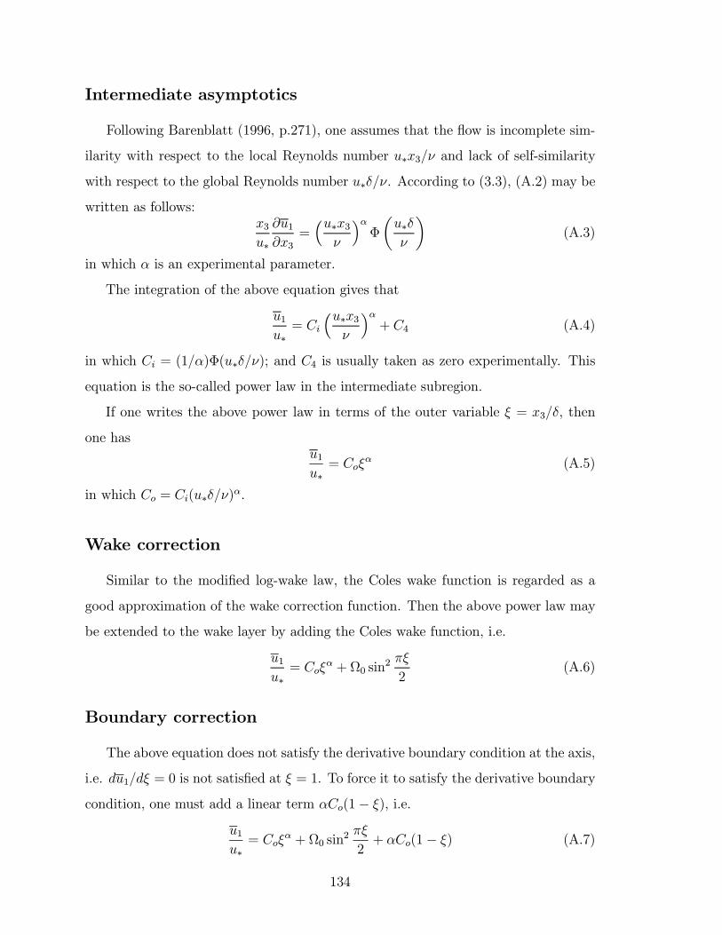
Intermediate asymptotics
Following Barenblatt (1996, p.271), one assumes that the ßow is incomplete sim-
ilarity with respect to the local Reynolds number u∗x3/ν and lack of self-similarity
with respect to the global Reynolds number u∗δ/ν. According to (3.3), (A.2) may be
written as follows:x3u∗
∂u1∂x3
=³u∗x3ν
´αΦ
µu∗δν
¶(A.3)
in which α is an experimental parameter.
The integration of the above equation gives that
u1u∗= Ci
³u∗x3ν
´α+ C4 (A.4)
in which Ci = (1/α)Φ(u∗δ/ν); and C4 is usually taken as zero experimentally. This
equation is the so-called power law in the intermediate subregion.
If one writes the above power law in terms of the outer variable ξ = x3/δ, then
one hasu1u∗= Coξ
α (A.5)
in which Co = Ci(u∗δ/ν)α.
Wake correction
Similar to the modiÞed log-wake law, the Coles wake function is regarded as a
good approximation of the wake correction function. Then the above power law may
be extended to the wake layer by adding the Coles wake function, i.e.
u1u∗= Coξ
α + Ω0 sin2 πξ
2(A.6)
Boundary correction
The above equation does not satisfy the derivative boundary condition at the axis,
i.e. du1/dξ = 0 is not satisÞed at ξ = 1. To force it to satisfy the derivative boundary
condition, one must add a linear term αCo(1− ξ), i.e.u1u∗= Coξ
α + Ω0 sin2 πξ
2+ αCo(1− ξ) (A.7)
134
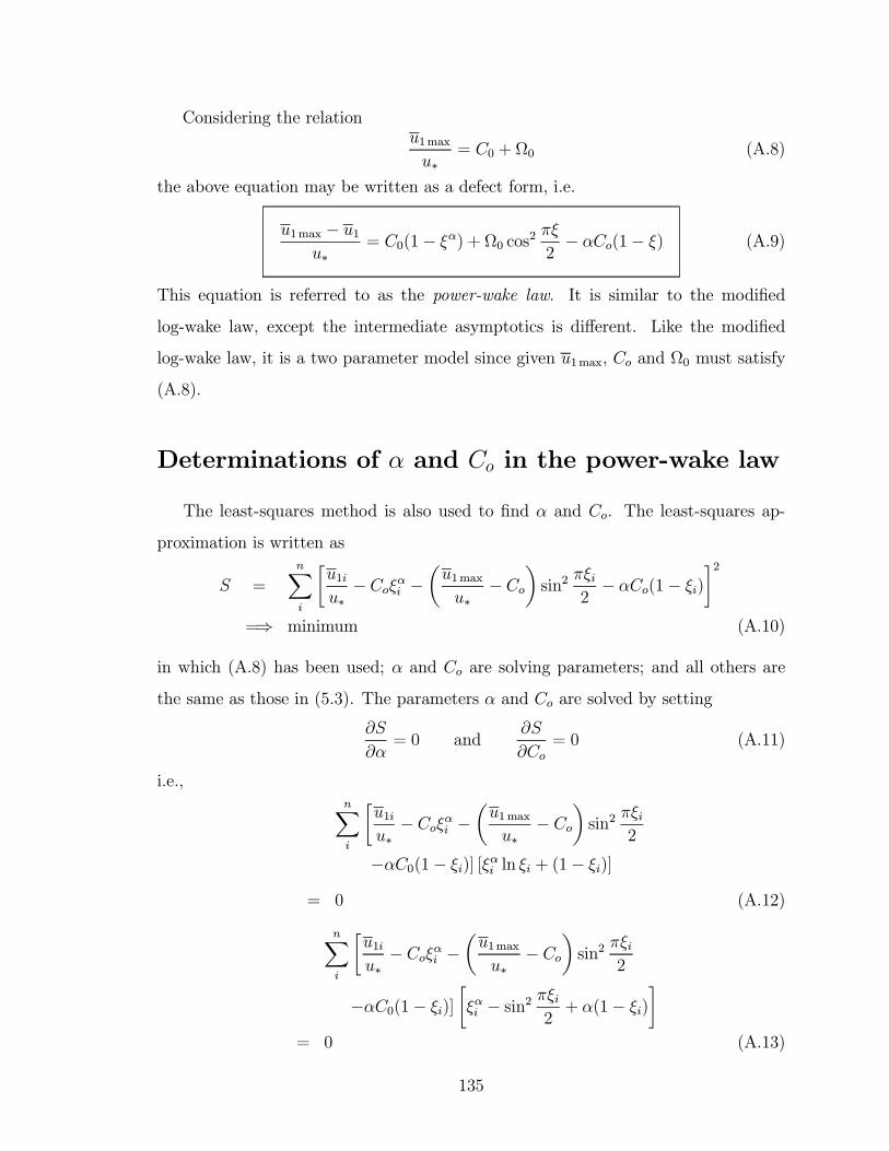
Considering the relationu1maxu∗
= C0 + Ω0 (A.8)
the above equation may be written as a defect form, i.e.
u1max − u1u∗
= C0(1− ξα) + Ω0 cos2 πξ2− αCo(1− ξ) (A.9)
This equation is referred to as the power-wake law. It is similar to the modiÞed
log-wake law, except the intermediate asymptotics is different. Like the modiÞed
log-wake law, it is a two parameter model since given u1max, Co and Ω0 must satisfy
(A.8).
Determinations of α and Co in the power-wake law
The least-squares method is also used to Þnd α and Co. The least-squares ap-
proximation is written as
S =nXi
·u1iu∗− Coξαi −
µu1maxu∗
− Co¶sin2
πξi2− αCo(1− ξi)
¸2=⇒ minimum (A.10)
in which (A.8) has been used; α and Co are solving parameters; and all others are
the same as those in (5.3). The parameters α and Co are solved by setting
∂S
∂α= 0 and
∂S
∂Co= 0 (A.11)
i.e.,nXi
·u1iu∗− Coξαi −
µu1maxu∗
− Co¶sin2
πξi2
−αC0(1− ξi)] [ξαi ln ξi + (1− ξi)]= 0 (A.12)
nXi
·u1iu∗− Coξαi −
µu1maxu∗
− Co¶sin2
πξi2
−αC0(1− ξi)]·ξαi − sin2
πξi2+ α(1− ξi)
¸= 0 (A.13)
135
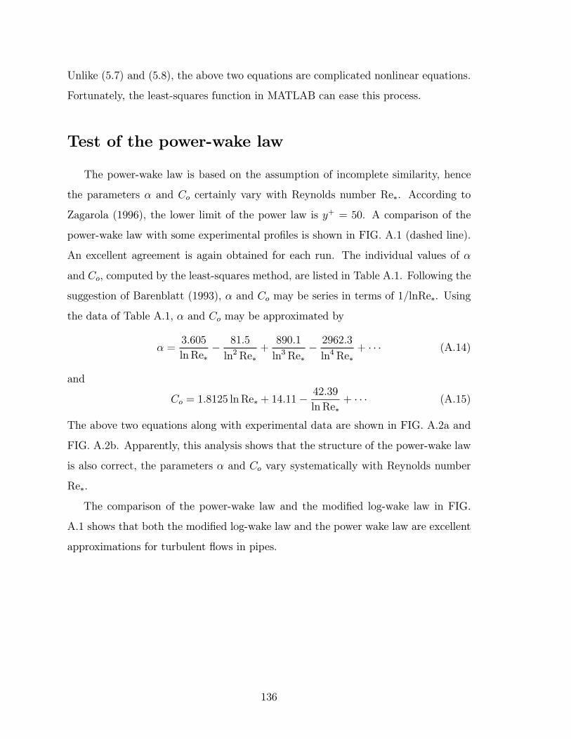
Unlike (5.7) and (5.8), the above two equations are complicated nonlinear equations.
Fortunately, the least-squares function in MATLAB can ease this process.
Test of the power-wake law
The power-wake law is based on the assumption of incomplete similarity, hence
the parameters α and Co certainly vary with Reynolds number Re∗. According to
Zagarola (1996), the lower limit of the power law is y+ = 50. A comparison of the
power-wake law with some experimental proÞles is shown in FIG. A.1 (dashed line).
An excellent agreement is again obtained for each run. The individual values of α
and Co, computed by the least-squares method, are listed in Table A.1. Following the
suggestion of Barenblatt (1993), α and Co may be series in terms of 1/lnRe∗. Using
the data of Table A.1, α and Co may be approximated by
α =3.605
lnRe∗− 81.5
ln2Re∗+890.1
ln3Re∗− 2962.3
ln4Re∗+ · · · (A.14)
and
Co = 1.8125 lnRe∗ + 14.11− 42.39
lnRe∗+ · · · (A.15)
The above two equations along with experimental data are shown in FIG. A.2a and
FIG. A.2b. Apparently, this analysis shows that the structure of the power-wake law
is also correct, the parameters α and Co vary systematically with Reynolds number
Re∗.
The comparison of the power-wake law and the modiÞed log-wake law in FIG.
A.1 shows that both the modiÞed log-wake law and the power wake law are excellent
approximations for turbulent ßows in pipes.
136
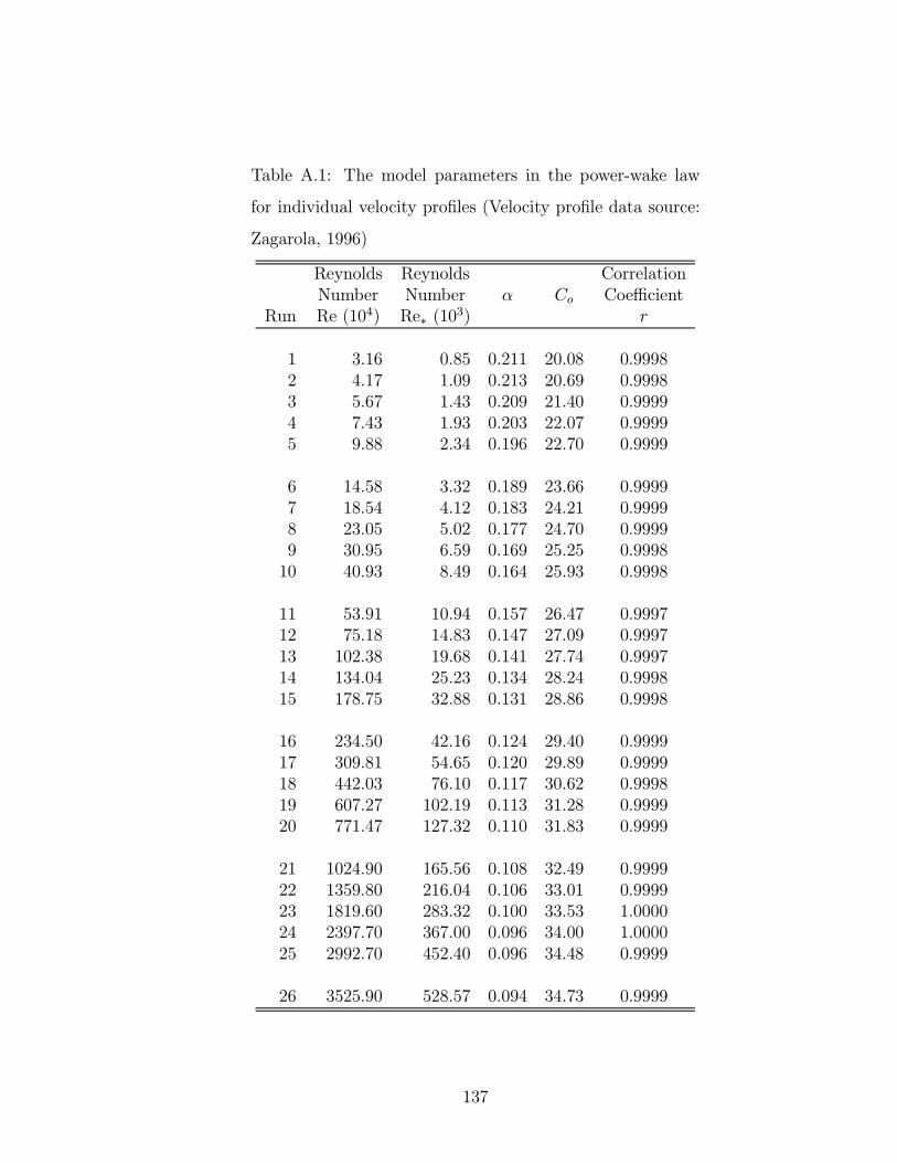
Table A.1: The model parameters in the power-wake law
for individual velocity proÞles (Velocity proÞle data source:
Zagarola, 1996)
Reynolds Reynolds CorrelationNumber Number α Co Coefficient
Run Re (104) Re∗ (103) r
1 3.16 0.85 0.211 20.08 0.99982 4.17 1.09 0.213 20.69 0.99983 5.67 1.43 0.209 21.40 0.99994 7.43 1.93 0.203 22.07 0.99995 9.88 2.34 0.196 22.70 0.9999
6 14.58 3.32 0.189 23.66 0.99997 18.54 4.12 0.183 24.21 0.99998 23.05 5.02 0.177 24.70 0.99999 30.95 6.59 0.169 25.25 0.999810 40.93 8.49 0.164 25.93 0.9998
11 53.91 10.94 0.157 26.47 0.999712 75.18 14.83 0.147 27.09 0.999713 102.38 19.68 0.141 27.74 0.999714 134.04 25.23 0.134 28.24 0.999815 178.75 32.88 0.131 28.86 0.9998
16 234.50 42.16 0.124 29.40 0.999917 309.81 54.65 0.120 29.89 0.999918 442.03 76.10 0.117 30.62 0.999819 607.27 102.19 0.113 31.28 0.999920 771.47 127.32 0.110 31.83 0.9999
21 1024.90 165.56 0.108 32.49 0.999922 1359.80 216.04 0.106 33.01 0.999923 1819.60 283.32 0.100 33.53 1.000024 2397.70 367.00 0.096 34.00 1.000025 2992.70 452.40 0.096 34.48 0.9999
26 3525.90 528.57 0.094 34.73 0.9999
137
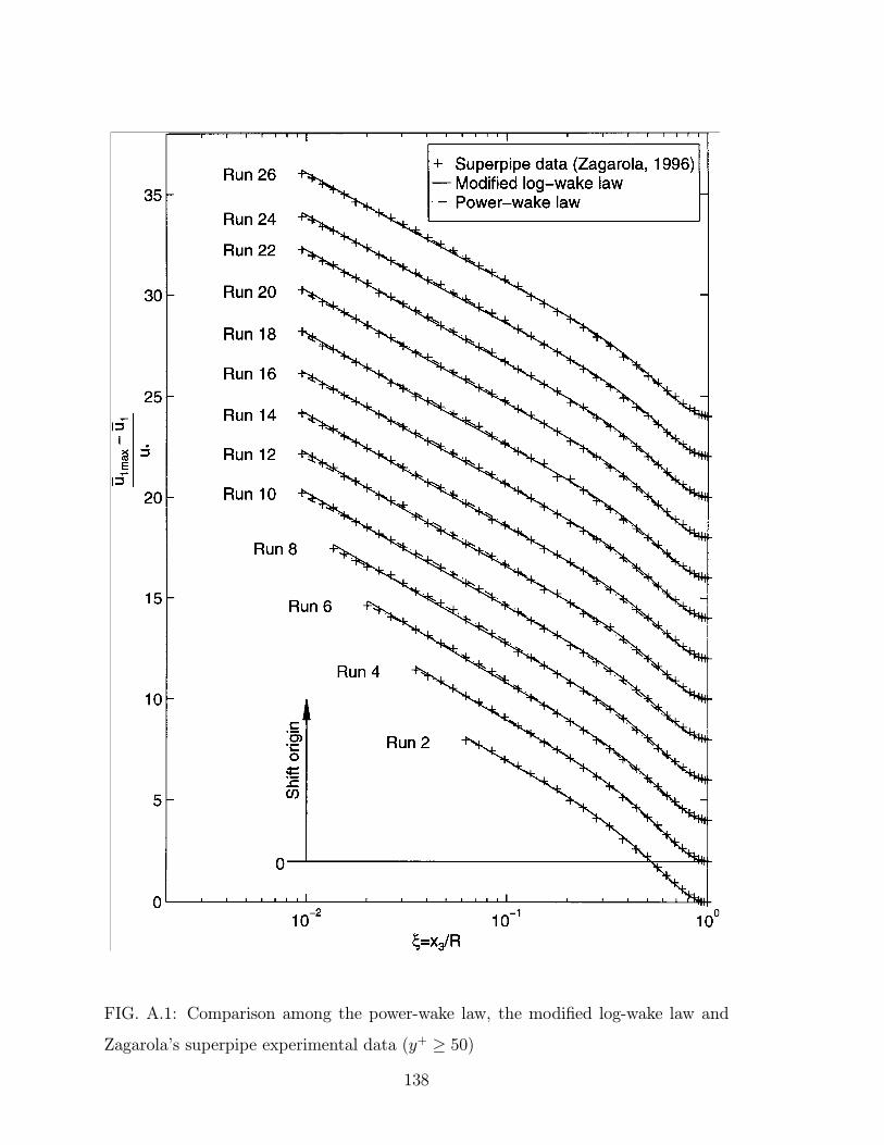
FIG. A.1: Comparison among the power-wake law, the modiÞed log-wake law and
Zagarolas superpipe experimental data (y+ ≥ 50)138
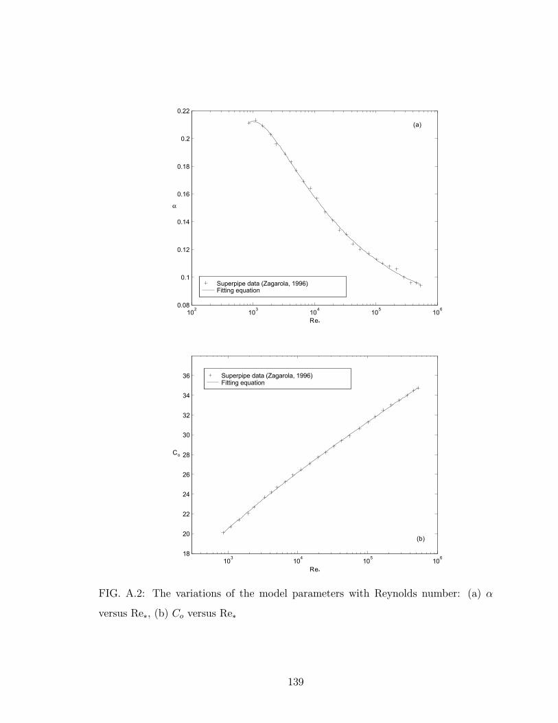
Superpipe data (Zagarola, 1996)Fitting equation
102 103 104 105 1060.08
0.1
0.12
0.14
0.16
0.18
0.2
0.22
Re*
α
(a)
Superpipe data (Zagarola, 1996)Fitting equation
103 104 105 10618
20
22
24
26
28
30
32
34
36
Re*
Co
(b)
FIG. A.2: The variations of the model parameters with Reynolds number: (a) α
versus Re∗, (b) Co versus Re∗
139
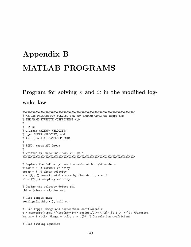
Appendix B
MATLAB PROGRAMS
Program for solving κ and Ω in the modiÞed log-
wake law
%%%%%%%%%%%%%%%%%%%%%%%%%%%%%%%%%%%%%%%%%%%%%%%%%%%%%%%%%%%%%%%%%%%%%
% MATLAB PROGRAM FOR SOLVING THE VON KARMAN CONSTANT kappa AND
% THE WAKE STRENGTH COEFFICIENT W_0
%
% GIVEN:
% u_1max: MAXIMUM VELOCITY;
% u_*: SHEAR VELOCITY; and
% (xi_i, u_1i): SAMPLE POINTS.
%
% FIND: kappa AND Omega
%
% Written by Junke Guo, Mar. 20, 1997
%%%%%%%%%%%%%%%%%%%%%%%%%%%%%%%%%%%%%%%%%%%%%%%%%%%%%%%%%%%%%%%%%%%%%
% Replace the following question marks with right numbers
u1max = ?; % maximum velocity
ustar = ?; % shear velocity
x = [?]; % normalized distance by flow depth, x = xi
u1 = [?]; % sampling velocity
% Define the velocity defect phi
phi = (u1max - u1)./ustar;
% Plot sample data
semilogx(x,phi,+), hold on
% Find kappa, Omega and correlation coefficient r
p = curvefit(x,phi,[-log(x)-(1-x) cos(pi./2.*x).^2],[1 1 0 +]); %Function
kappa = 1./p(1); Omega = p(2); r = p(3); % Correlation coefficient
% Plot fitting equation
140
x = logspace(log10(0.005),0,100);
y = p(1).*(-log(x)-(1-x)) + p(2).*cos(pi./2.*x).^2;
semilogx(x,y,r), hold off
legend(Measured data,Modified log-wake law)
sxlabel(\xi = x_3/R)
sylabel(\fracu\left6.7\up5\-_1max \- u\left6.7\up5\-_1u_*)
%xxxxxxxxxxxxxxxxxxxxxxxxxxxxxxxxxxxxxxxxxxxxxxxxxxxxxxxxxxxxxxxxxxxx
function pr=curvefit(x,y,arg3,options)
%%%%%%%%%%%%%%%%%%%%%%%%%%%%%%%%%%%%%%%%%%%%%%%%%%%%%%%%%%%%%%%%%%%%%
% CURVEFIT Curve fitting and plotting routine
% pr = [parameters_fitted; corrcoef].
%
% CURVEFIT(X,Y) plots the points specified by the vectors
% X and Y using the symbol *, and simultaneously plots a
% straight line that represents the best linear fit to
% the data.
%
% CURVEFIT(X,Y,N) for integer N fits an Nth order polynomial
% to the data.
%
% CURVEFIT(X,Y,[F1(x) F2(x) ...]) fits Y to the closest
% linear combinations of the vectors F1(x), F2(x), etc.
% This is useful for fitting arbitrary functions of X to Y.
% (Ie. curvefit(X,Y,[exp(X) cos(2*X)])
%
% P=CURVEFIT(X,Y,...) returns the estimated fitting
% coefficients in the vector P. In the polynomial fitting case,
% the P coefficients are ordered highest order first (slope,
% then y-intercept in the 1st order case).
%
% CURVEFIT(X,Y,N,OPTIONS) allow the caller to specify certain
% options. If OPTIONS(1)=1, then no plot is generated. This
% useful if the caller is only interested in the returned
% values. If OPTIONS(2)=1, then the X-axis is plotted on
% a log scale. If OPTIONS(3)=1, then the Y-axis is plotted on
% a log scale. If OPTIONS(4) is specified, its value is
% assumed to be a character representing the symbol to use
% to plot the original data, which has a default value of *.
% This element can be set to the character i for invisible if
% only the best-fit curve is desired in the plot.
%
% Written by Junke Guo, Dec. 29, 1996
%%%%%%%%%%%%%%%%%%%%%%%%%%%%%%%%%%%%%%%%%%%%%%%%%%%%%%%%%%%%%%%%%%%%%%%%%%
if nargin<2, error(too few arguements); end
f = [];
if nargin<4,
options=[0 0 0 *];
else
options=options(:); %Forces options to be a row vector
% This zeros all non-existent terms.
141
if length(options)<4, options(4)=*; end
end
% Regulate input data to columns
x = x(:); y = y(:);
if nargin<3,
N=1; % Fit a straight line
else
% if arg3 is a scalar, set N to it.
[r,c]=size(arg3);
if max([r,c])==1, N=arg3;
else
f=eval(arg3);
end
end
if isempty(f),
P = polyfit(x,y,N);
yfitted = polyval(P,x);
else
% Determine the size of f
[r c] = size(f);
N = c;
% Determine the matrix of linear system equations
for j=1:N
for k=1:N, a = f(:,j).*f(:,k); A(j,k) = sum(a); end
b = f(:,j).*y; B(j) = sum(b);
end
B = B(:);
% Determine the fitted coefficients
P = A\B;
% Determine the fitted values of y
yfitted = f*P;
end
% Calculate correlation coefficient
R = corrcoef(y,yfitted); R = R(1,2);
if options(1)~=1, % If we are plotting...
% Determine which plot command to use.
if options(2)==0,
if options(3)==0,
plotcmd = plot;
else
plotcmd = semilogy;
end
else
if options(3)==0,
plotcmd = semilogx;
142
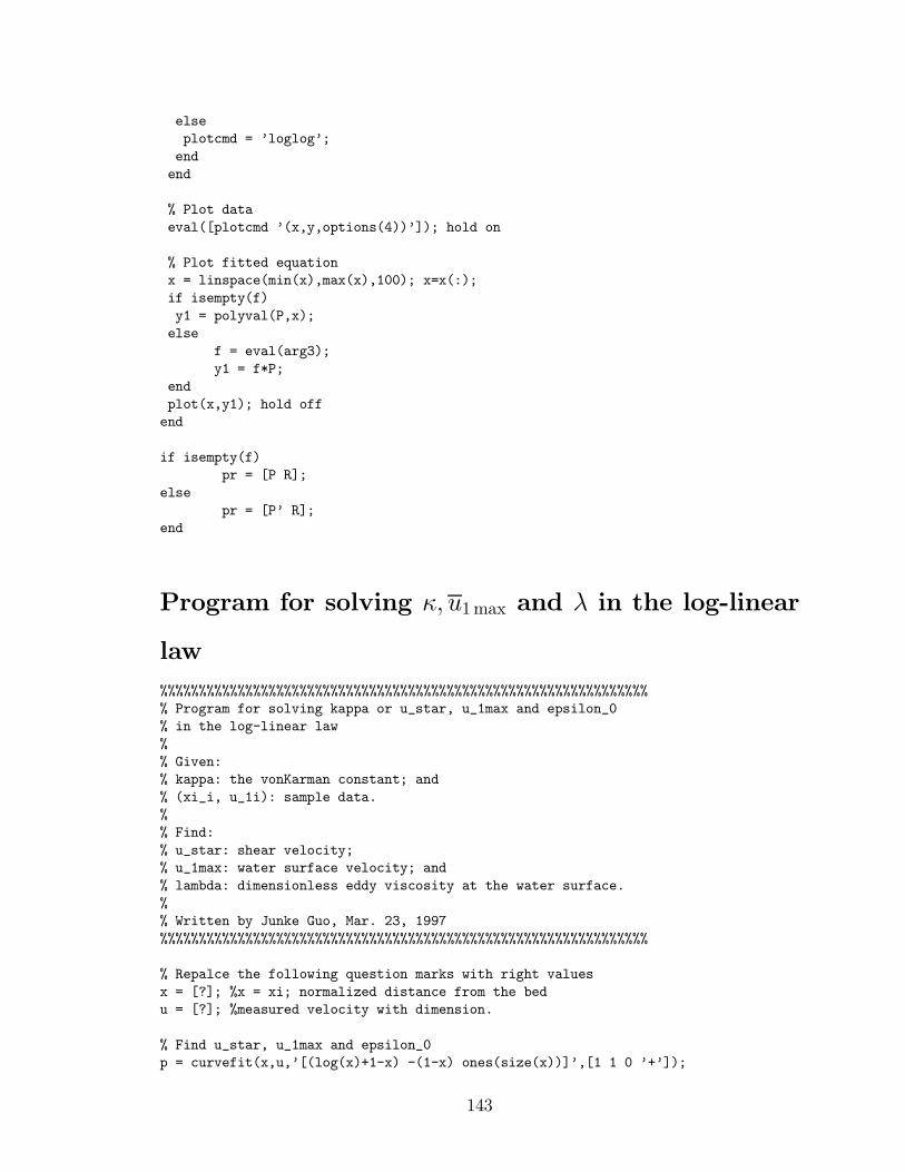
else
plotcmd = loglog;
end
end
% Plot data
eval([plotcmd (x,y,options(4))]); hold on
% Plot fitted equation
x = linspace(min(x),max(x),100); x=x(:);
if isempty(f)
y1 = polyval(P,x);
else
f = eval(arg3);
y1 = f*P;
end
plot(x,y1); hold off
end
if isempty(f)
pr = [P R];
else
pr = [P R];
end
Program for solving κ, u1max and λ in the log-linear
law
%%%%%%%%%%%%%%%%%%%%%%%%%%%%%%%%%%%%%%%%%%%%%%%%%%%%%%%%%%%%%%%
% Program for solving kappa or u_star, u_1max and epsilon_0
% in the log-linear law
%
% Given:
% kappa: the vonKarman constant; and
% (xi_i, u_1i): sample data.
%
% Find:
% u_star: shear velocity;
% u_1max: water surface velocity; and
% lambda: dimensionless eddy viscosity at the water surface.
%
% Written by Junke Guo, Mar. 23, 1997
%%%%%%%%%%%%%%%%%%%%%%%%%%%%%%%%%%%%%%%%%%%%%%%%%%%%%%%%%%%%%%%
% Repalce the following question marks with right values
x = [?]; %x = xi; normalized distance from the bed
u = [?]; %measured velocity with dimension.
% Find u_star, u_1max and epsilon_0
p = curvefit(x,u,[(log(x)+1-x) -(1-x) ones(size(x))],[1 1 0 +]);
143
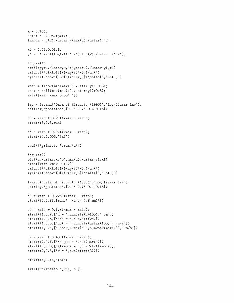
k = 0.406;
ustar = 0.406.*p(1);
lambda = p(2)./ustar./(max(u)./ustar).^2;
x1 = 0.01:0.01:1;
y1 = -1./k.*(log(x1)+1-x1) + p(2)./ustar.*(1-x1);
figure(1)
semilogy(u./ustar,x,o,max(u)./ustar-y1,x1)
sxlabel(u\left7\up7\-_1/u_*)
sylabel(\down-30\fracx_3\delta,Rot,0)
xmin = floor(min(max(u)./ustar-y1)-0.5);
xmax = ceil(max(max(u)./ustar-y1)+0.5);
axis([xmin xmax 0.004 4])
leg = legend(Data of Kironoto (1993),Log-linear law);
set(leg,position,[0.15 0.75 0.4 0.15])
t3 = xmin + 0.2.*(xmax - xmin);
stext(t3,0.3,run)
t4 = xmin + 0.9.*(xmax - xmin);
stext(t4,0.008,(a))
eval([printsto ,run,a])
figure(2)
plot(u./ustar,x,o,max(u)./ustar-y1,x1)
axis([xmin xmax 0 1.2])
sxlabel(u\left7\up7\-_1/u_*)
sylabel(\down0\fracx_3\delta,Rot,0)
legend(Data of Kironoto (1993),Log-linear law)
set(leg,position,[0.15 0.75 0.4 0.15])
t0 = xmin + 0.225.*(xmax - xmin);
stext(t0,0.85,[run, (k_s= 4.8 mm)])
t1 = xmin + 0.1.*(xmax - xmin);
stext(t1,0.7,[h = ,num2str(h*100), cm])
stext(t1,0.6,[a/h = ,num2str(wh)])
stext(t1,0.5,[u_* = ,num2str(ustar*100), cm/s])
stext(t1,0.4,[u\bar_1max= ,num2str(max(u)), m/s])
t2 = xmin + 0.43.*(xmax - xmin);
stext(t2,0.7,[\kappa = ,num2str(k)])
stext(t2,0.6,[\lambda = ,num2str(lambda)])
stext(t2,0.5,[r = ,num2str(p(3))])
stext(t4,0.14,(b))
eval([printsto ,run,b])
144
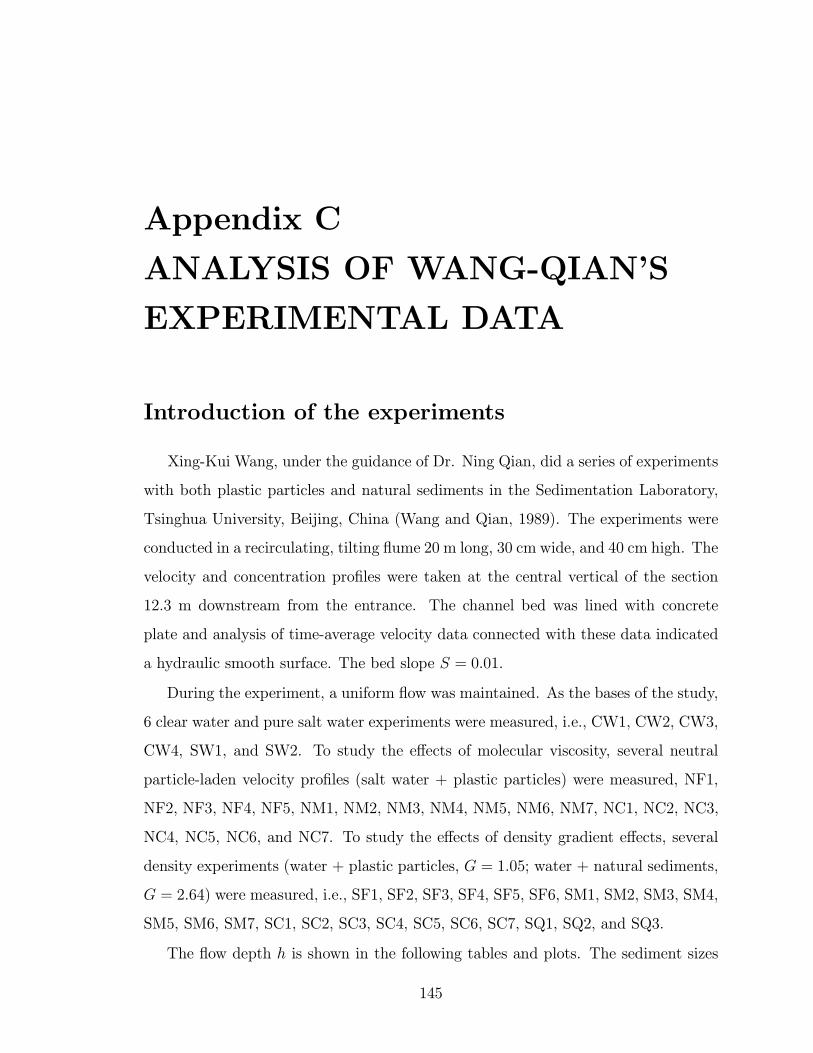
Appendix C
ANALYSIS OF WANG-QIANS
EXPERIMENTAL DATA
Introduction of the experiments
Xing-Kui Wang, under the guidance of Dr. Ning Qian, did a series of experiments
with both plastic particles and natural sediments in the Sedimentation Laboratory,
Tsinghua University, Beijing, China (Wang and Qian, 1989). The experiments were
conducted in a recirculating, tilting ßume 20 m long, 30 cm wide, and 40 cm high. The
velocity and concentration proÞles were taken at the central vertical of the section
12.3 m downstream from the entrance. The channel bed was lined with concrete
plate and analysis of time-average velocity data connected with these data indicated
a hydraulic smooth surface. The bed slope S = 0.01.
During the experiment, a uniform ßow was maintained. As the bases of the study,
6 clear water and pure salt water experiments were measured, i.e., CW1, CW2, CW3,
CW4, SW1, and SW2. To study the effects of molecular viscosity, several neutral
particle-laden velocity proÞles (salt water + plastic particles) were measured, NF1,
NF2, NF3, NF4, NF5, NM1, NM2, NM3, NM4, NM5, NM6, NM7, NC1, NC2, NC3,
NC4, NC5, NC6, and NC7. To study the effects of density gradient effects, several
density experiments (water + plastic particles, G = 1.05; water + natural sediments,
G = 2.64) were measured, i.e., SF1, SF2, SF3, SF4, SF5, SF6, SM1, SM2, SM3, SM4,
SM5, SM6, SM7, SC1, SC2, SC3, SC4, SC5, SC6, SC7, SQ1, SQ2, and SQ3.
The ßow depth h is shown in the following tables and plots. The sediment sizes
145
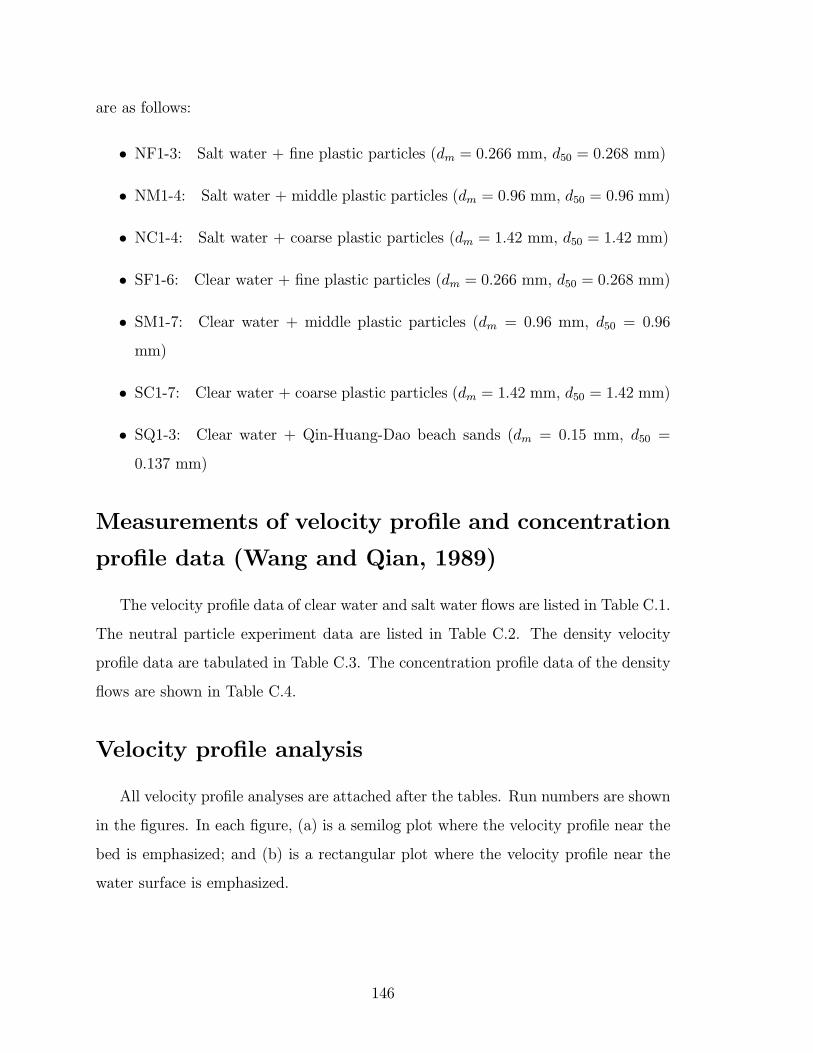
are as follows:
NF1-3: Salt water + Þne plastic particles (dm = 0.266 mm, d50 = 0.268 mm)
NM1-4: Salt water + middle plastic particles (dm = 0.96 mm, d50 = 0.96 mm)
NC1-4: Salt water + coarse plastic particles (dm = 1.42 mm, d50 = 1.42 mm)
SF1-6: Clear water + Þne plastic particles (dm = 0.266 mm, d50 = 0.268 mm)
SM1-7: Clear water + middle plastic particles (dm = 0.96 mm, d50 = 0.96
mm)
SC1-7: Clear water + coarse plastic particles (dm = 1.42 mm, d50 = 1.42 mm)
SQ1-3: Clear water + Qin-Huang-Dao beach sands (dm = 0.15 mm, d50 =
0.137 mm)
Measurements of velocity proÞle and concentration
proÞle data (Wang and Qian, 1989)
The velocity proÞle data of clear water and salt water ßows are listed in Table C.1.
The neutral particle experiment data are listed in Table C.2. The density velocity
proÞle data are tabulated in Table C.3. The concentration proÞle data of the density
ßows are shown in Table C.4.
Velocity proÞle analysis
All velocity proÞle analyses are attached after the tables. Run numbers are shown
in the Þgures. In each Þgure, (a) is a semilog plot where the velocity proÞle near the
bed is emphasized; and (b) is a rectangular plot where the velocity proÞle near the
water surface is emphasized.
146
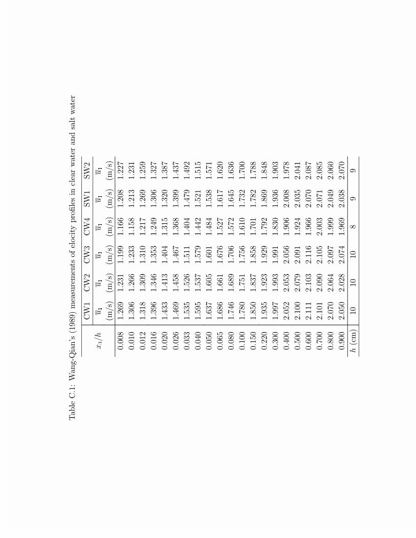
!
"
#
$
%
%"
&&&&&&
'''
"(
"#
((
"'
"")
'''
#'(
"((
"##
*
"#
"#
''"
#
#'
#'
")
"(
"*
''(
#(
#$(
#*#
"$
#'(
#")
''"'
$##
$#
$'$
#*
#"'
#)
''"(
$(
$*
$()
#(
#
$#)
''##
*#*
*"(
*
$'$
$)
$"
''$'
**
*#)
*)
$$"
*"
**
''*'
(#)
('*
('
$$
*#
*)
''(*
((
((
()(
*")
()
("'
'''
)$(
(
)'(
*)"
($*
(#(
'''
)'
)*
)*(
('
)#"
)''
'*'
*'
#)
*
)'
)"
)
'""'
#*
"#
"
)"
(
$
'#''
)
#
#'
#(
'#
'$''
"'*"
"'*#
"'*(
'(
"''
)
'*''
"''
"')
"'
"$
"'#*
"'$
'(''
"
"'#
"(
((
"')'
"')
')''
"'
"''
"'*
"''#
"')
"'*
'''
"')'
"'($
"')
"'$
"'('
'''
"'*'
"'"
"')$
(
"'#
"')'
''
'
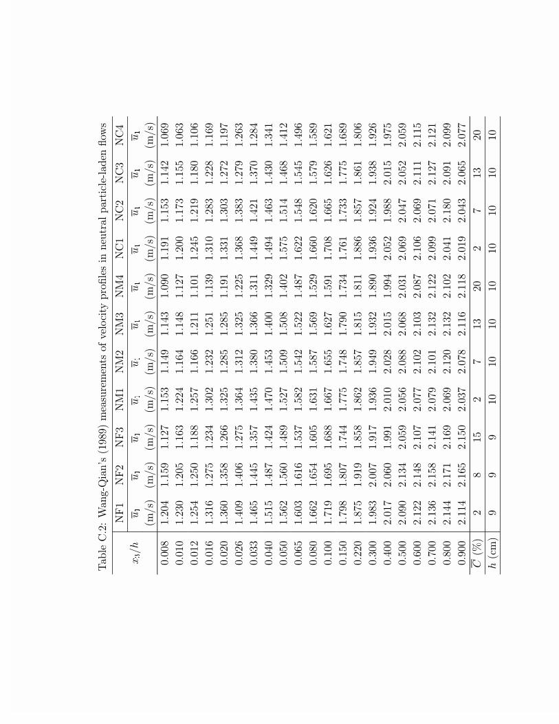
" + !,
-.
-."
-.#
-/
-/"
-/#
-/$
-
-"
-#
-$
&&&&&&&&&&&
'''
"'$
*
")
*#
$
$#
''
*#
$"
'(
'''
"#'
"'*
(#
""$
($
$
")
"''
)#
**
'(#
''"
"*$
"*'
"*)
((
"
'
"$*
"
'
'(
''(
#(
")*
"#$
#'"
"#"
"*
#
#'
"#
""
(
''"'
#('
#*
"((
#"*
"*
"*
##
#'#
")"
)
''"(
$'
$'(
")*
#($
#"
#"*
""*
#(
##
")
"(#
''##
$(*
$$*
#*)
$#*
#'
#((
#
$$
$"
#)'
"$
''$'
**
$)
$"$
$)'
$*#
$''
#"
$$
$(#
$#'
#$
''*'
*("
*('
$
*")
*'
*'
$'"
*)*
*$
$(
$"
''(*
('#
((
*#)
*"
*$"
*""
$)
(""
*$
*$*
$(
'''
(("
(*$
('*
(#
*)
*(
*"
(('
("'
*)
*
'''
)
(*
(
(()
(**
(")
*
)'
((*
("(
("
'*'
)
')
)$$
))*
)$
)'
)#$
)(
)##
))*
(
'""'
)*
*
("
*)
*
(
*)
(
'(
'#''
#
"'')
)
#(
$
#"
'
#(
"$
#
"(
'$''
"')
"'('
"''
"'"
"'*
$
"'*"
"'*
)*
'*''
"''
"#$
"'*
"'*(
"'
"'(
"'#
"'(
"'$)
"'*"
"'*
'(''
"""
"$
"')
"'))
"'"
"'#
"')
"'(
"'(
"
"*
')''
"#(
"*
"$
"')
"'
"#"
"""
"'
"')
"")
""
'''
"$$
")
"(
"'(
""'
"#"
"'"
"'$
"'
"'
"'
'''
"$
"(*
"*'
"'#)
"')
"(
"
"'
"'$#
"'(*
"'))
0
"
*"
)#
"'"
)#
"'
'
''
''
''
'
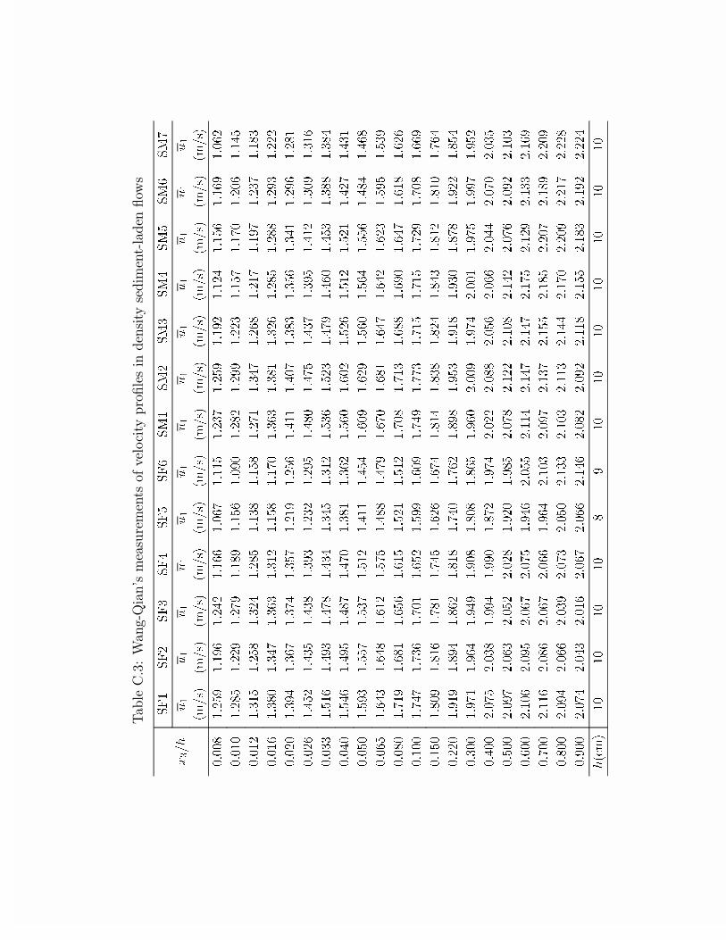
# +!! !,
VI4
VI5
VI6
VI7
VI8
VI9
VP4
VP5
VP6
VP7
VP8
VP9
VP:
@k
x
x
x
x
x
x
x
x
x
x
x
x
x
+p2v,
+p2v,
+p2v,
+p2v,
+p2v,
+p2v,
+p2v,
+p2v,
+p2v,
+p2v,
+p2v,
+p2v,
+p2v,
3133;
4158<
414<9
41575
41499
4139:
41448
4156:
4158<
414<5
41457
41489
4149<
41395
31343
415;8
4155<
415:<
414;<
41489
413<3
415;5
415<<
41556
4148:
414:3
41539
41478
31345
41648
4158;
41657
415;8
4146;
4148;
415:4
4167:
4159;
4154:
414<:
4156:
414;6
31349
416;3
4167:
41696
41645
4148;
414:3
41696
416;4
41659
415;8
415;;
415<6
41555
31353
416<7
4169:
416:7
4168:
4154<
41589
41744
4173:
416;6
41689
41674
415<9
415;4
31359
41785
41768
4176;
416<6
41565
415<8
417;3
417:8
4176:
416<8
41745
4163<
41649
31366
41849
417<6
417:;
41767
41678
41645
41869
41856
417:<
41793
41786
416;;
416;7
31373
41879
417<8
417;:
417:3
416;4
41695
41893
41935
41859
41845
41854
4175:
41764
31383
418<6
4188:
4186:
41845
41744
41787
4193<
4195<
41893
41897
41889
417;7
4179;
31398
41976
4197;
41945
418:8
417;;
417:<
419:3
419;4
4197:
41975
41956
418<8
4186<
313;3
41:4<
419;4
41989
41948
41854
41845
41:3;
41:46
419;;
419<3
4197:
4194;
41959
31433
41:7:
41:69
41:34
41985
418<<
4193<
41:7<
41::6
41:48
41:48
41:5<
41:3;
4199<
31483
41;3<
41;49
41:;4
41:78
41959
419:7
41;47
41;6;
41;57
41;76
41;45
41;43
41:97
31553
41<4<
41;<7
41;95
41;4;
41:73
41:95
41;<;
41<86
41<4;
41<63
41;:;
41<55
41;87
31633
41<:4
41<97
41<7<
41<3;
41;3;
41;98
41<93
5133<
41<:7
51334
41<:8
41<<:
41<85
31733
513:8
5136;
41<<7
41<<3
41;:5
41<:7
51355
513;;
51389
51399
51377
513:3
51368
31833
513<:
51396
51385
5135;
41<53
41<;8
513:;
51455
5143;
51475
513:9
513<5
51436
31933
51439
513<8
5139:
513:8
41<79
51388
51447
5147:
5147:
514:8
5145<
51466
5149<
31:33
51449
513;9
5139:
51399
41<97
51436
513<:
5146:
51488
514;8
5153:
514;<
5153<
31;33
513<7
51399
5136<
513:6
51383
51466
51436
51446
51477
514:3
5153<
5154:
5155;
31<33
513:7
51376
51349
5139:
51399
51479
513;5
513<5
5144;
51488
514;6
514<5
51557
k+fp,
43
43
43
43
;<
43
43
43
43
43
43
43
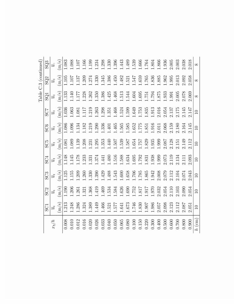
#!
%
%"
%#
%$
%*
%(
%)
%
%"
%#
&&&&&&&&&&
'''
"#
'
"*
$
'
'(
'#(
##
'*
'#
'''
"$
"'(
**
$*
'
'(
'(#
$'
')
'
''"
"(
"(
"'
)
#
#$
'
))
#)
')
''(
#"$
#"
"('
"##
"'
"
)
""
"'
((
''"'
#
#(
##'
##
"#
"
"
"("
")$
''"(
$$
$
#'
#)$
"*
"'
"(#
#*'
##'
"#$
''##
$((
$(
$"
$$
#*#
##(
"
#(
#$*
"
''$'
*"
*#$
$
$'
$$'
$'
#*
$"*
#(
##'
''*'
*))
*$
*$#
*(
*')
$(*
$(
$(
$*'
#(
''(*
($
("(
(''
*
*#
*(*
*"$
*#
$"
$$#
'''
()#
('
(*
(#$
*)
**
*
*$$
*"
$
'''
)$(
)*"
)'(
(*
(*$
(*"
($
('$
*$)
*#
'*'
#'
)
)*
)"
)*)
))*
)*#
(*
(*
(((
'""'
')
)
(*
#
"
*
#*
)*
)(*
)($
'#''
(
)'
$"
#
#*
(
#
)$
#(
'$
'$''
"'*)
"'#"
"''
"'
"'(
)*
*
((
'*''
"'
"'*$
"')
"')#
"')
"'(
"'*$
##
("
#(
'(''
""#
"'
""
"
""
"*
"#)
*
"''*
')''
""
"'#
"'$
"#$
"*
"'
")*
"''*
"'#
"''#
'''
"')
"''
"')$
"
"$
"($
"$*
"')
"'"
"'#
'''
"'*
"'*$
"'$#
"'#
""
"$*
"$)
"'(
"'*
"'
''
''
''
'
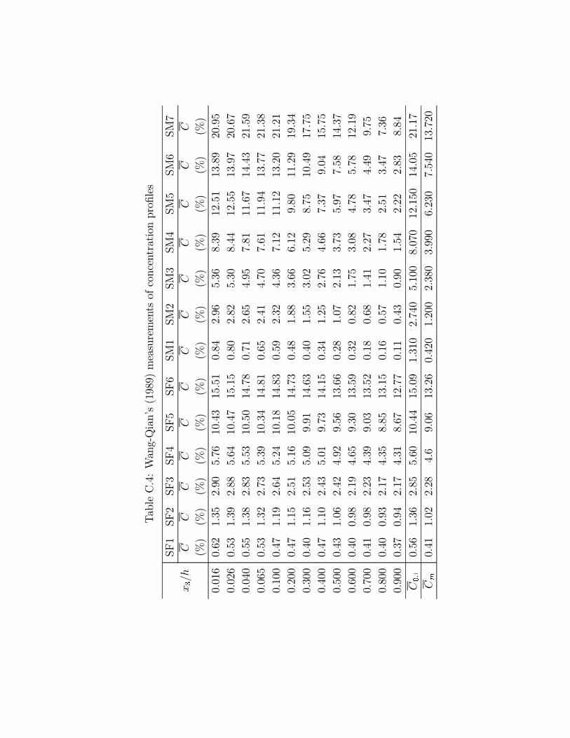
$
%.
%."
%.#
%.$
%.*
%.(
%/
%/"
%/#
%/$
%/*
%/(
%/)
0
0
0
0
0
0
0
0
0
0
0
0
0
''(
'("
#*
"'
*)(
'$#
**
'$
"(
*#(
#
"*
#
"'*
''"(
'*#
#
"
*($
'$)
**
''
""
*#'
$$
"**
#)
"'()
''$'
'**
#
"#
**#
'*'
$)
')
"(*
$*
)
()
$$#
"*
''(*
'*#
#"
")#
*#
'#$
$
'(*
"$
$)'
)(
$
#))
"#
'''
'$)
"($
*"$
'
$#
'*
"#"
$#(
)"
"
#"'
""
'"''
'$)
*
"*
*(
''*
$)#
'$
#((
("
'
"
#$
'#''
'$'
(
"*#
*'
$(#
'$'
**
#'"
*"
)*
'$
))*
'$''
'$)
'
"$#
*'
)#
$*
'#$
"*
")(
$((
)#)
'$
*)*
'*''
'$#
'(
"$"
$"
*(
#((
'"
')
"#
#)#
*)
)*
$#)
'(''
'$'
'
"
$(*
#'
#*
'#"
'"
)*
#'
$)
*)
"
')''
'$
'
""#
$#
'#
#*"
'
'(
$
"")
#$)
$$
)*
'''
'$'
'#
")
$#*
*
#*
'(
'*)
'
)
"*
#$)
)#(
'''
'#)
'$
")
$#
()
"))
'
'$#
''
*$
"""
"#
$
f
'*(
#(
"*
*('
'$$
*'
#'
")$'
*''
')'
"*'
$'*
")
6
'$
'"
""
$(
'(
#"(
'$"'
"''
"#'
#'
("#'
)*$'
#)"'
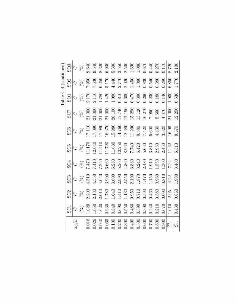
$!
%
%"
%#
%$
%*
%(
%)
%
%"
%#
0
0
0
0
0
0
0
0
0
0
''(
'"'
""''
$*'
)$)'
)'
)'
"'''
")'
)*'
($'
''"(
'*'
"#'
$#*'
)$'
"($'
)''
"'''
"'
)(#'
*$'
''$'
'"'
"''
$'$'
)"*'
$'
)''
"'''
)'
("*'
#"'
''(*
'#'
)'
#''
((('
)"'
(#)'
"'''
$"'
*)'
(#'
'''
'$'
($'
#(''
("'
(#'
*'
"'''
''
$$$'
**'
'"''
'('
$'
"'
*"('
'"*'
$)('
))$'
''
"))'
#**'
'#''
'**'
#'
"**'
$#('
('
"('
)'
'(''
"'"'
"*''
'$''
'$'
'*'
"'
##'
))$'
"''
*"'
'$)'
$*'
('
'*''
'#'
')'
)'
#"$'
($"'
*'
#"'
'#'
''
''
'(''
'#''
'*'
$)'
"$'
*'('
)$"'
'")'
'"'
'#'
'()'
')''
'"$'
'$('
*'
'
#'
*(''
)*'
'"#'
'*$'
'$$'
'''
'"'
'#'
'('
**'
"('
$$#'
*(('
''
'#'
'")'
'''
'')'
'''
''
#''
"$('
##"'
$#)'
'$'
'"'
')'
''
"'*
$""
)"$
("
((
"'''
''
(*'
)"'
6
'$#'
'*'
'
#$''
(*'
#)'
""*'
'*#'
))'
"''

Dat
a of
Wan
g-Q
ian
(198
9)M
odifi
ed lo
g-w
ake
law
1214
1618
2022
24
10-2
10-1
100
u− 1/u*
x 3 δ___
CW
1
(a)
y+ =
70
1214
1618
2022
240
0.2
0.4
0.6
0.81
1.2
1.4
1.6
u− 1/u *
x 3 δ___
CW
1
h =
10 c
m
a/h
= 3
δ =
6.36
2 cm
δ /h
= 0.
6362
u 1m
ax =
2.1
09 m
/s
u * =
9.1
61 c
m/s
κ 0 =
0.4
186
Ω0
= 1.
324
r = 0
.999
2
(b)
Dat
a of
Wan
g-Q
ian
(198
9)M
odifi
ed lo
g-w
ake
law
1214
1618
2022
24
10-2
10-1
100
u− 1/u*
x 3 δ___
CW
2
(a)
y+ =
70
1214
1618
2022
240
0.2
0.4
0.6
0.81
1.2
1.4
1.6
u− 1/u *
x 3 δ___
CW
2
h =
10 c
m
a/h
= 3
δ =
6.25
4 cm
δ /h
= 0.
6254
u 1m
ax =
2.0
98 m
/s
u * =
9.1
61 c
m/s
κ 0 =
0.4
123
Ω0
= 1.
49
r = 0
.999
4
(b)

Dat
a of
Wan
g-Q
ian
(198
9)M
odifi
ed lo
g-w
ake
law
1015
2025
10-2
10-1
100
u− 1/u*
x 3 δ___
CW
3
(a)
y+ =
70
1015
2025
0
0.51
1.5
u− 1/u *
x 3 δ___
CW
3
h =
10 c
m
a/h
= 3
δ =
6.71
2 cm
δ /h
= 0.
6712
u 1m
ax =
2.1
15 m
/s
u * =
9.1
61 c
m/s
κ 0 =
0.3
897
Ω0
= 1.
202
r = 0
.999
6
(b)
Dat
a of
Wan
g-Q
ian
(198
9)M
odifi
ed lo
g-w
ake
law
1214
1618
2022
24
10-2
10-1
100
u− 1/u*
x 3 δ___
CW
4
(a)
y+ =
70
1214
1618
2022
240
0.2
0.4
0.6
0.81
1.2
1.4
u− 1/u *
x 3 δ___
CW
4
h =
8 cm
a/h
= 3.
75
δ =
6.05
9 cm
δ /h
= 0.
7574
u 1m
ax =
1.9
93 m
/s
u * =
8.4
05 c
m/s
κ 0 =
0.4
121
Ω0
= 1.
698
r = 0
.999
3
(b)
Dat
a of
Wan
g-Q
ian
(198
9)M
odifi
ed lo
g-w
ake
law
1214
1618
2022
24
10-2
10-1
100
u− 1/u*
x 3 δ___
SW
1
(a)
y+ =
70
1214
1618
2022
240
0.51
1.5
u− 1/u *
x 3 δ___
SW
1
h =
9 cm
a/h
= 3.
333
δ =
6.18
6 cm
δ /h
= 0.
6874
u 1m
ax =
2.0
71 m
/s
u * =
8.8
05 c
m/s
κ 0 =
0.3
854
Ω0
= 1.
447
r = 0
.998
7
(b)
Dat
a of
Wan
g-Q
ian
(198
9)M
odifi
ed lo
g-w
ake
law
1214
1618
2022
24
10-2
10-1
100
u− 1/u*
x 3 δ___
SW
2
(a)
y+ =
70
1214
1618
2022
240
0.2
0.4
0.6
0.81
1.2
1.4
u− 1/u *
x 3 δ___
SW
2
h =
9 cm
a/h
= 3.
333
δ =
6.51
2 cm
δ /h
= 0.
7235
u 1m
ax =
2.0
89 m
/s
u * =
8.8
05 c
m/s
κ 0 =
0.4
237
Ω0
= 1.
906
r = 0
.999
3
(b)
Dat
a of
Wan
g-Q
ian
(198
9)M
odifi
ed lo
g-w
ake
law
1214
1618
2022
2426
10-2
10-1
100
u− 1/u*
x 3 δ___
NF1
(a)
y+ =
70
1214
1618
2022
2426
0
0.2
0.4
0.6
0.81
1.2
1.4
u− 1/u *
x 3 δ___
NF1
h =
9 cm
a/h
= 3.
333
δ =
6.77
4 cm
δ/h
= 0.
7526
C =
0.0
2
u 1m
ax =
2.1
38 m
/s
u * =
8.8
05 c
m/s
κ =
0.38
87
Ω =
1.9
62
r = 0
.999
4
(b)
Dat
a of
Wan
g-Q
ian
(198
9)M
odifi
ed lo
g-w
ake
law
1214
1618
2022
2426
10-2
10-1
100
u− 1/u*
x 3 δ___
NF2
(a)
y+ =
70
1214
1618
2022
2426
0
0.2
0.4
0.6
0.81
1.2
u− 1/u *
x 3 δ___
NF2
h =
9 cm
a/h
= 3.
333
δ =
6.99
9 cm
δ /h
= 0.
7776
C =
0.0
8
u 1m
ax =
2.1
72 m
/s
u * =
8.8
05 c
m/s
κ =
0.35
53
Ω =
1.8
81
r = 0
.998
7
(b)
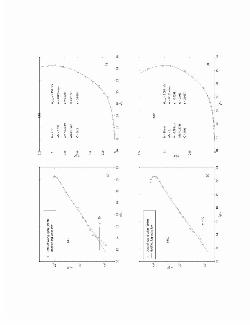
Dat
a of
Wan
g-Q
ian
(198
9)M
odifi
ed lo
g-w
ake
law
1012
1416
1820
2224
26
10-2
10-1
100
u− 1/u*
x 3 δ___
NF3
(a)
y+ =
70
1012
1416
1820
2224
260
0.2
0.4
0.6
0.81
1.2
u− 1/u *
x 3 δ___
NF3
h =
9 cm
a/h
= 3.
333
δ =
7.61
5 cm
δ /h
= 0.
8461
C =
0.1
5
u 1m
ax =
2.1
59 m
/s
u * =
8.8
05 c
m/s
κ =
0.33
94
Ω =
2.1
22
r = 0
.998
4
(b)
Dat
a of
Wan
g-Q
ian
(198
9)M
odifi
ed lo
g-w
ake
law
1012
1416
1820
2224
10-2
10-1
100
u− 1/u*
x 3 δ___
NM
1
(a)
y+ =
70
1012
1416
1820
2224
0
0.51
1.5
u− 1/u *
x 3 δ___
NM
1
h =
10 c
m
a/h
= 3
δ =
6.78
5 cm
δ /h
= 0.
6785
C =
0.0
2
u 1m
ax =
2.0
84 m
/s
u * =
9.1
61 c
m/s
κ =
0.41
91
Ω =
2.0
13
r = 0
.998
7
(b)
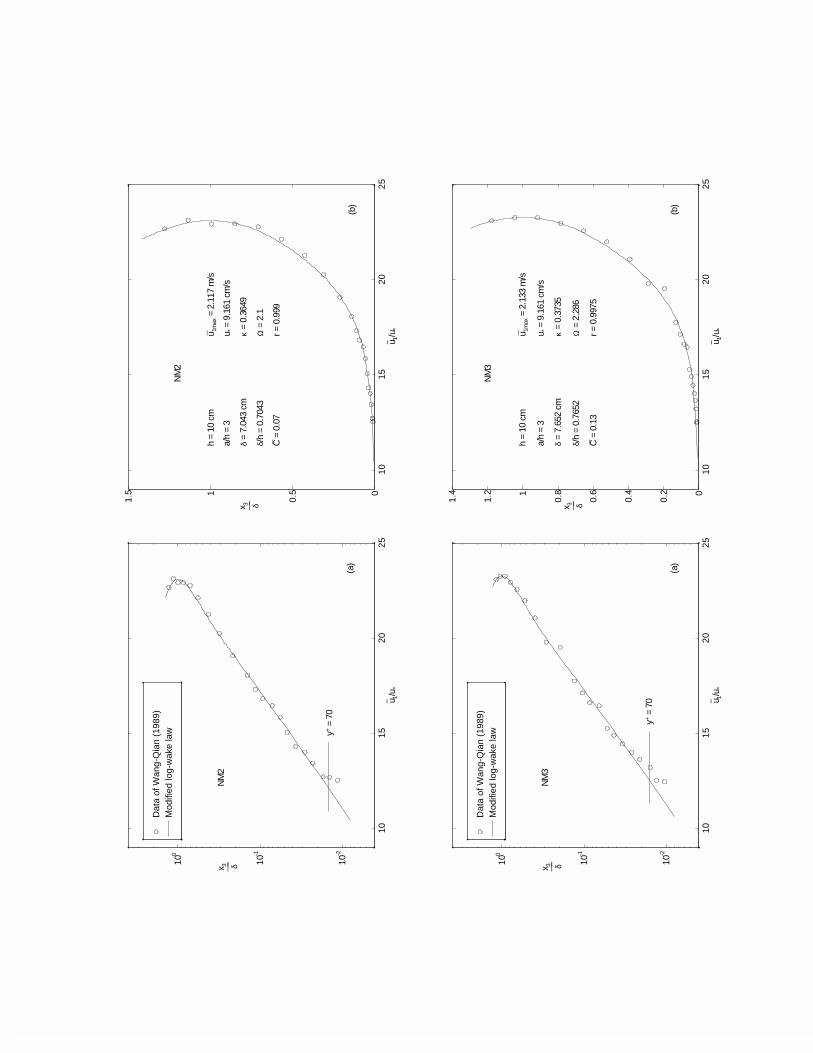
Dat
a of
Wan
g-Q
ian
(198
9)M
odifi
ed lo
g-w
ake
law
1015
2025
10-2
10-1
100
u− 1/u*
x 3 δ___
NM
2
(a)
y+ =
70
1015
2025
0
0.51
1.5
u− 1/u *
x 3 δ___
NM
2
h =
10 c
m
a/h
= 3
δ =
7.04
3 cm
δ /h
= 0.
7043
C =
0.0
7
u 1m
ax =
2.1
17 m
/s
u * =
9.1
61 c
m/s
κ =
0.36
49
Ω =
2.1
r = 0
.999
(b)
Dat
a of
Wan
g-Q
ian
(198
9)M
odifi
ed lo
g-w
ake
law
1015
2025
10-2
10-1
100
u− 1/u*
x 3 δ___
NM
3
(a)
y+ =
70
1015
2025
0
0.2
0.4
0.6
0.81
1.2
1.4
u− 1/u *
x 3 δ___
NM
3
h =
10 c
m
a/h
= 3
δ =
7.65
2 cm
δ /h
= 0.
7652
C =
0.1
3
u 1m
ax =
2.1
33 m
/s
u * =
9.1
61 c
m/s
κ =
0.37
35
Ω =
2.2
86
r = 0
.997
5
(b)
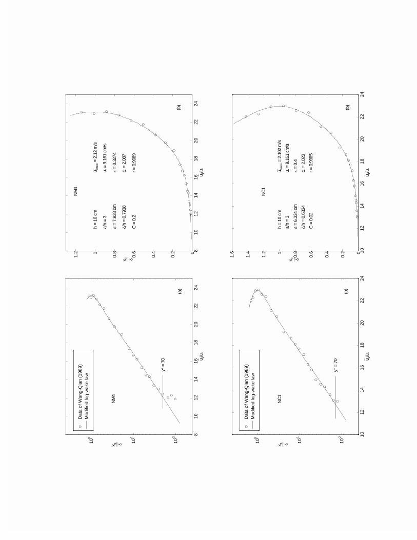
Dat
a of
Wan
g-Q
ian
(198
9)M
odifi
ed lo
g-w
ake
law
810
1214
1618
2022
24
10-2
10-1
100
u− 1/u*
x 3 δ___
NM
4
(a)
y+ =
70
810
1214
1618
2022
240
0.2
0.4
0.6
0.81
1.2
u− 1/u *
x 3 δ___
NM
4
h =
10 c
m
a/h
= 3
δ =
7.93
8 cm
δ /h
= 0.
7938
C =
0.2
u 1m
ax =
2.1
2 m
/s
u * =
9.1
61 c
m/s
κ =
0.32
74
Ω =
2.0
87
r = 0
.998
9
(b)
Dat
a of
Wan
g-Q
ian
(198
9)M
odifi
ed lo
g-w
ake
law
1012
1416
1820
2224
10-2
10-1
100
u− 1/u*
x 3 δ___
NC
1
(a)
y+ =
70
1012
1416
1820
2224
0
0.2
0.4
0.6
0.81
1.2
1.4
1.6
u− 1/u *
x 3 δ___
NC
1
h =
10 c
m
a/h
= 3
δ =
6.33
4 cm
δ /h
= 0.
6334
C =
0.0
2
u 1m
ax =
2.1
02 m
/s
u * =
9.1
61 c
m/s
κ =
0.4
Ω =
2.0
23
r = 0
.998
5
(b)

Dat
a of
Wan
g-Q
ian
(198
9)M
odifi
ed lo
g-w
ake
law
1012
1416
1820
2224
10-2
10-1
100
u− 1/u*
x 3 δ___
NC
2
(a)
y+ =
70
1012
1416
1820
2224
0
0.2
0.4
0.6
0.81
1.2
1.4
u− 1/u *
x 3 δ___
NC
2
h =
10 c
m
a/h
= 3
δ =
7.44
3 cm
δ/h
= 0.
7443
C =
0.0
7
u 1m
ax =
2.1
04 m
/s
u * =
9.1
61 c
m/s
κ =
0.40
93
Ω =
2.1
14
r = 0
.996
8
(b)
Dat
a of
Wan
g-Q
ian
(198
9)M
odifi
ed lo
g-w
ake
law
1015
2025
10-2
10-1
100
u− 1/u*
x 3 δ___
NC
3
(a)
y+ =
70
1015
2025
0
0.51
1.5
u− 1/u *
x 3 δ___
NC
3
h =
10 c
m
a/h
= 3
δ =
6.94
4 cm
δ /h
= 0.
6944
C =
0.1
3
u 1m
ax =
2.1
13 m
/s
u * =
9.1
61 c
m/s
κ =
0.35
25
Ω =
2.0
95
r = 0
.998
4
(b)
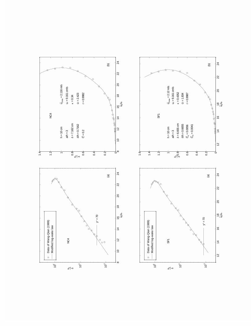
Dat
a of
Wan
g-Q
ian
(198
9)M
odifi
ed lo
g-w
ake
law
810
1214
1618
2022
24
10-2
10-1
100
u− 1/u*
x 3 δ___
NC
4
(a)
y+ =
70
810
1214
1618
2022
240
0.2
0.4
0.6
0.81
1.2
1.4
u− 1/u *
x 3 δ___
NC
4
h =
10 c
m
a/h
= 3
δ =
7.16
2 cm
δ/h
= 0.
7162
C =
0.2
u 1m
ax =
2.1
16 m
/s
u * =
9.1
61 c
m/s
κ =
0.34
Ω =
2.4
23
r = 0
.998
2
(b)
Dat
a of
Wan
g-Q
ian
(198
9)M
odifi
ed lo
g-w
ake
law
1214
1618
2022
24
10-2
10-1
100
u− 1/u*
x 3 δ___
SF1
(a)
y+ =
70
1214
1618
2022
240
0.2
0.4
0.6
0.81
1.2
1.4
1.6
u− 1/u *
x 3 δ___
SF1
h =
10 c
m
a/h
= 3
δ =
6.65
5 cm
δ /h
= 0.
6655
Ca
= 0.
0056
Cm =
0.0
041
u 1m
ax =
2.1
2 m
/s
u * =
9.1
61 c
m/s
κ =
0.43
52
Ω =
1.8
34
r = 0
.998
7
(b)
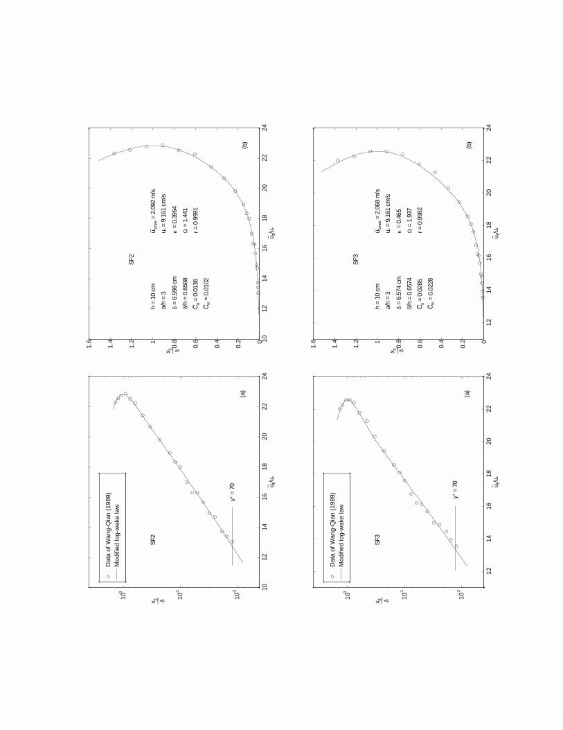
Dat
a of
Wan
g-Q
ian
(198
9)M
odifi
ed lo
g-w
ake
law
1012
1416
1820
2224
10-2
10-1
100
u− 1/u*
x 3 δ___
SF2
(a)
y+ =
70
1012
1416
1820
2224
0
0.2
0.4
0.6
0.81
1.2
1.4
1.6
u− 1/u *
x 3 δ___
SF2
h =
10 c
m
a/h
= 3
δ =
6.59
8 cm
δ /h
= 0.
6598
Ca
= 0.
0136
Cm =
0.0
102
u 1m
ax =
2.0
92 m
/s
u * =
9.1
61 c
m/s
κ =
0.39
64
Ω =
1.4
41
r = 0
.999
1
(b)
Dat
a of
Wan
g-Q
ian
(198
9)M
odifi
ed lo
g-w
ake
law
1214
1618
2022
24
10-2
10-1
100
u− 1/u*
x 3 δ___
SF3
(a)
y+ =
70
1214
1618
2022
240
0.2
0.4
0.6
0.81
1.2
1.4
1.6
u− 1/u *
x 3 δ___
SF3
h =
10 c
m
a/h
= 3
δ =
6.57
4 cm
δ /h
= 0.
6574
Ca
= 0.
0285
Cm =
0.0
228
u 1m
ax =
2.0
68 m
/s
u * =
9.1
61 c
m/s
κ =
0.46
5
Ω =
1.9
37
r = 0
.998
2
(b)
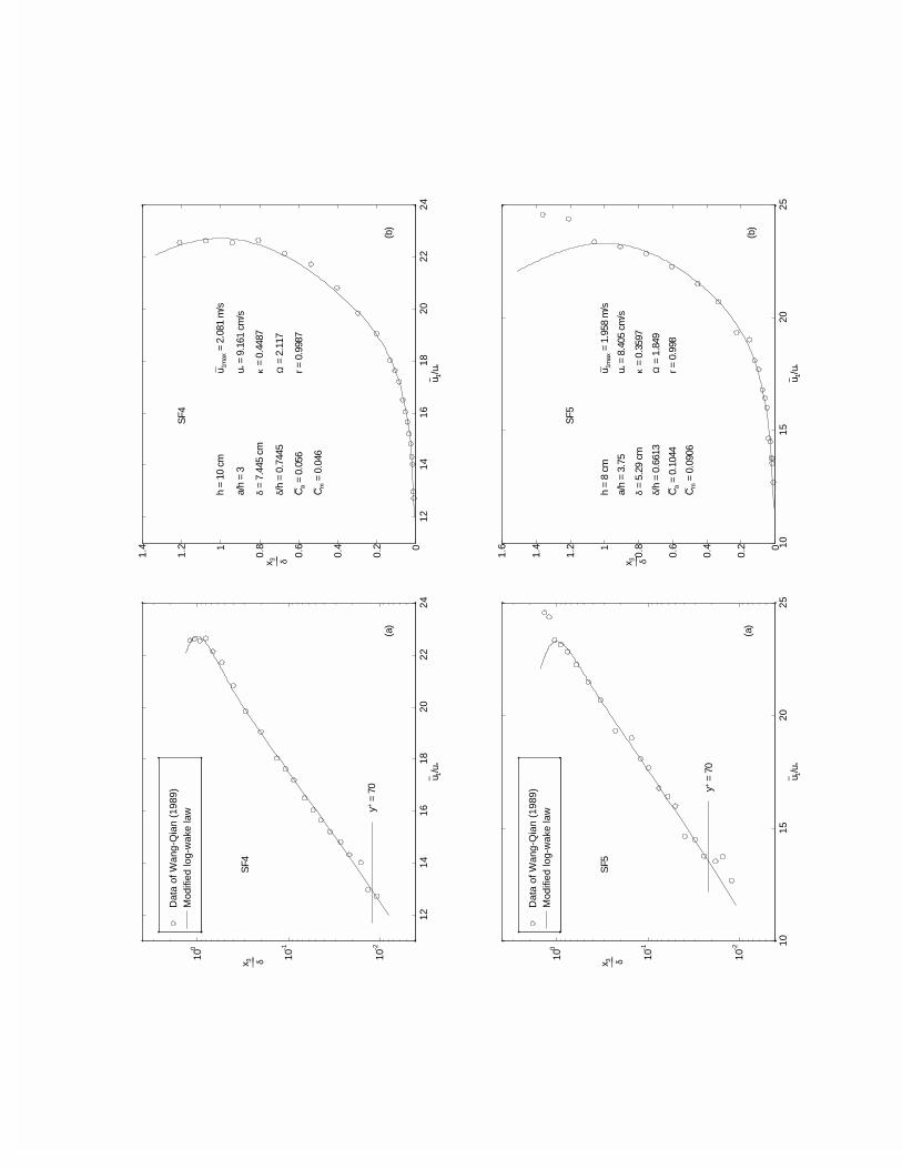
Dat
a of
Wan
g-Q
ian
(198
9)M
odifi
ed lo
g-w
ake
law
1214
1618
2022
24
10-2
10-1
100
u− 1/u*
x 3 δ___
SF4
(a)
y+ =
70
1214
1618
2022
240
0.2
0.4
0.6
0.81
1.2
1.4
u− 1/u *
x 3 δ___
SF4
h =
10 c
m
a/h
= 3
δ =
7.44
5 cm
δ/h
= 0.
7445
Ca
= 0.
056
Cm =
0.0
46
u 1m
ax =
2.0
81 m
/s
u * =
9.1
61 c
m/s
κ =
0.44
87
Ω =
2.1
17
r = 0
.998
7
(b)
Dat
a of
Wan
g-Q
ian
(198
9)M
odifi
ed lo
g-w
ake
law
1015
2025
10-2
10-1
100
u− 1/u*
x 3 δ___
SF5
(a)
y+ =
70
1015
2025
0
0.2
0.4
0.6
0.81
1.2
1.4
1.6
u− 1/u *
x 3 δ___
SF5
h =
8 cm
a/h
= 3.
75
δ =
5.29
cm
δ /h
= 0.
6613
Ca
= 0.
1044
Cm =
0.0
906
u 1m
ax =
1.9
58 m
/s
u * =
8.4
05 c
m/s
κ =
0.35
97
Ω =
1.8
49
r = 0
.998
(b)
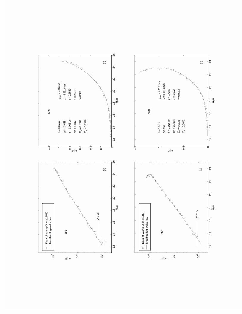
Dat
a of
Wan
g-Q
ian
(198
9)M
odifi
ed lo
g-w
ake
law
1214
1618
2022
2426
10-2
10-1
100
u− 1/u*
x 3 δ___
SF6
(a)
y+ =
70
1214
1618
2022
2426
0
0.2
0.4
0.6
0.81
1.2
u− 1/u *
x 3 δ___
SF6
h =
8.6
cm
a/h
= 3.
488
δ =
9.00
6 cm
δ/h
= 1.
047
Ca
= 0.
1509
Cm =
0.1
326
u 1m
ax =
2.1
6 m
/s
u * =
8.6
51 c
m/s
κ =
0.35
59
Ω =
2.5
07
r = 0
.998
(b)
Dat
a of
Wan
g-Q
ian
(198
9)M
odifi
ed lo
g-w
ake
law
1214
1618
2022
24
10-2
10-1
100
u− 1/u*
x 3 δ___
SM
1
(a)
y+ =
70
1214
1618
2022
240
0.51
1.5
u− 1/u *
x 3 δ___
SM
1
h =
10 c
m
a/h
= 3
δ =
7.06
4 cm
δ /h
= 0.
7064
Ca
= 0.
0131
Cm =
0.0
042
u 1m
ax =
2.1
12 m
/s
u * =
9.1
61 c
m/s
κ =
0.42
57
Ω =
1.5
02
r = 0
.999
2
(b)
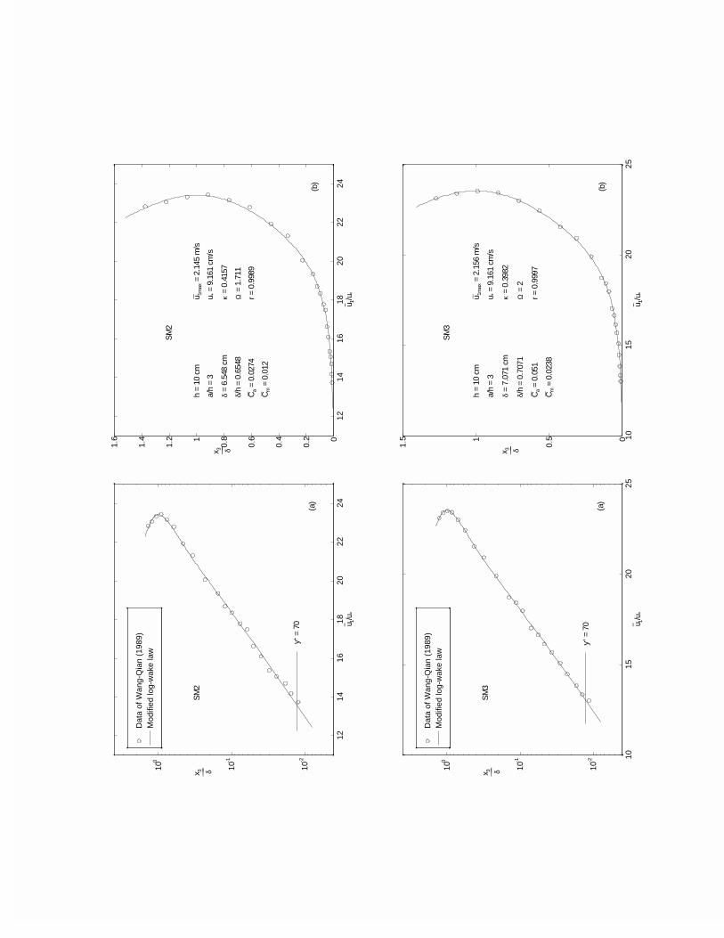
Dat
a of
Wan
g-Q
ian
(198
9)M
odifi
ed lo
g-w
ake
law
1214
1618
2022
24
10-2
10-1
100
u− 1/u*
x 3 δ___
SM
2
(a)
y+ =
70
1214
1618
2022
240
0.2
0.4
0.6
0.81
1.2
1.4
1.6
u− 1/u *
x 3 δ___
SM
2
h =
10 c
m
a/h
= 3
δ =
6.54
8 cm
δ /h
= 0.
6548
Ca
= 0.
0274
Cm =
0.0
12
u 1m
ax =
2.1
45 m
/s
u * =
9.1
61 c
m/s
κ =
0.41
57
Ω =
1.7
11
r = 0
.998
9
(b)
Dat
a of
Wan
g-Q
ian
(198
9)M
odifi
ed lo
g-w
ake
law
1015
2025
10-2
10-1
100
u− 1/u*
x 3 δ___
SM
3
(a)
y+ =
70
1015
2025
0
0.51
1.5
u− 1/u *
x 3 δ___
SM
3
h =
10 c
m
a/h
= 3
δ =
7.07
1 cm
δ /h
= 0.
7071
Ca
= 0.
051
Cm =
0.0
238
u 1m
ax =
2.1
56 m
/s
u * =
9.1
61 c
m/s
κ =
0.39
82
Ω =
2
r = 0
.999
7
(b)

Dat
a of
Wan
g-Q
ian
(198
9)M
odifi
ed lo
g-w
ake
law
1015
2025
10-2
10-1
100
u− 1/u*
x 3 δ___
SM
4
(a)
y+ =
70
1015
2025
0
0.2
0.4
0.6
0.81
1.2
1.4
u− 1/u *
x 3 δ___
SM
4
h =
10 c
m
a/h
= 3
δ =
7.18
7 cm
δ/h
= 0.
7187
Ca
= 0.
0807
Cm =
0.0
399
u 1m
ax =
2.1
86 m
/s
u * =
9.1
61 c
m/s
κ =
0.35
44
Ω =
1.8
67
r = 0
.999
7
(b)
Dat
a of
Wan
g-Q
ian
(198
9)M
odifi
ed lo
g-w
ake
law
1012
1416
1820
2224
26
10-2
10-1
100
u− 1/u*
x 3 δ___
SM
5
(a)
y+ =
70
1012
1416
1820
2224
260
0.2
0.4
0.6
0.81
1.2
u− 1/u *
x 3 δ___
SM
5
h =
10 c
m
a/h
= 3
δ =
8.83
cm
δ /h
= 0.
883
Ca
= 0.
1215
Cm =
0.0
623
u 1m
ax =
2.2
m/s
u * =
9.1
61 c
m/s
κ =
0.37
48
Ω =
1.9
02
r = 0
.999
1
(b)
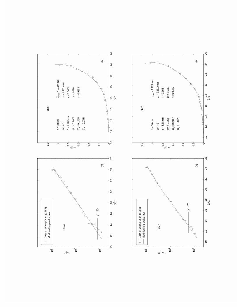
Dat
a of
Wan
g-Q
ian
(198
9)M
odifi
ed lo
g-w
ake
law
1012
1416
1820
2224
26
10-2
10-1
100
u− 1/u*
x 3 δ___
SM
6
(a)
y+ =
70
1012
1416
1820
2224
260
0.2
0.4
0.6
0.81
1.2
u− 1/u *
x 3 δ___
SM
6
h =
10 c
m
a/h
= 3
δ =
9.40
5 cm
δ/h
= 0.
9405
Ca
= 0.
1405
Cm =
0.0
754
u 1m
ax =
2.2
07 m
/s
u * =
9.1
61 c
m/s
κ =
0.34
84
Ω =
1.6
96
r = 0
.995
3
(b)
Dat
a of
Wan
g-Q
ian
(198
9)M
odifi
ed lo
g-w
ake
law
1012
1416
1820
2224
26
10-2
10-1
100
u− 1/u*
x 3 δ___
SM
7
(a)
y+ =
70
1012
1416
1820
2224
260
0.2
0.4
0.6
0.81
1.2
u− 1/u *
x 3 δ___
SM
7
h =
10 c
m
a/h
= 3
δ =
8.68
cm
δ /h
= 0.
868
Ca
= 0.
2117
Cm =
0.1
372
u 1m
ax =
2.2
29 m
/s
u * =
9.1
61 c
m/s
κ =
0.35
5
Ω =
2.6
76
r = 0
.999
5
(b)
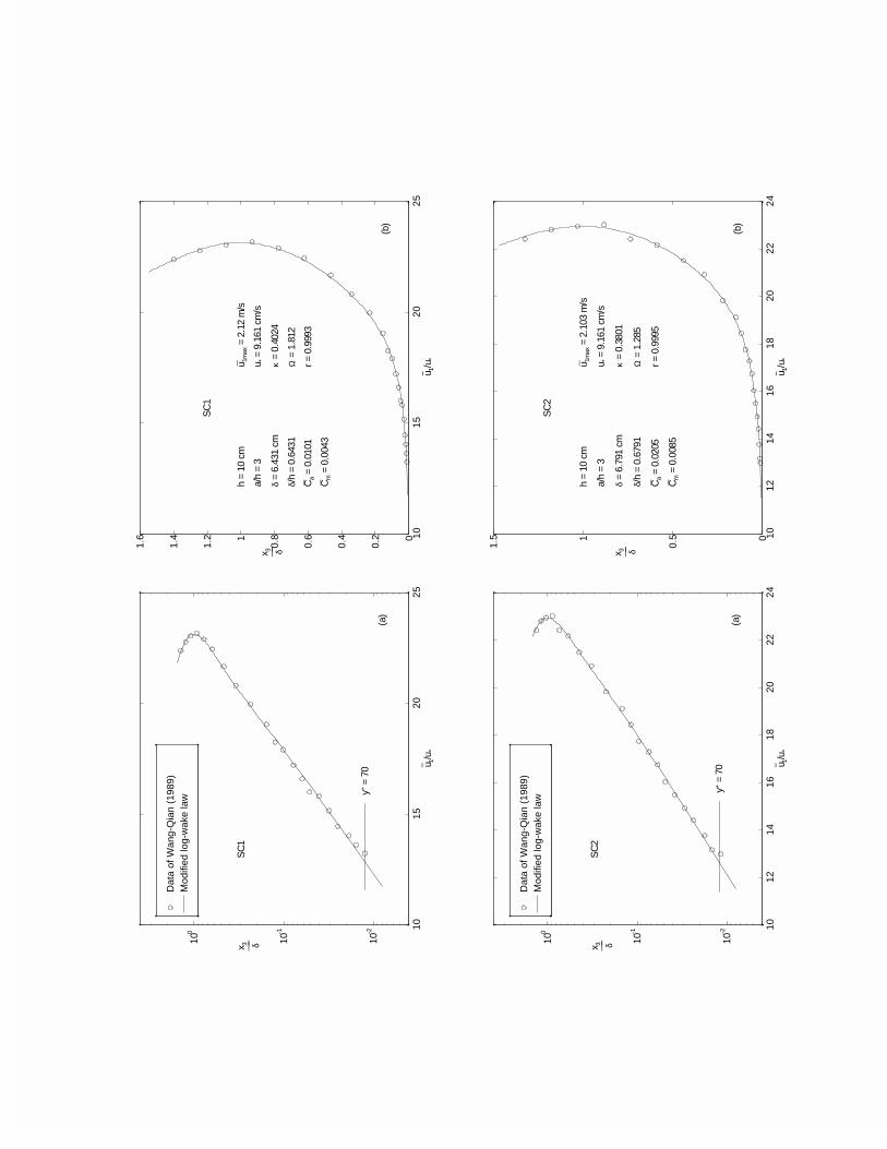
Dat
a of
Wan
g-Q
ian
(198
9)M
odifi
ed lo
g-w
ake
law
1015
2025
10-2
10-1
100
u− 1/u*
x 3 δ___
SC
1
(a)
y+ =
70
1015
2025
0
0.2
0.4
0.6
0.81
1.2
1.4
1.6
u− 1/u *
x 3 δ___
SC
1
h =
10 c
m
a/h
= 3
δ =
6.43
1 cm
δ /h
= 0.
6431
Ca
= 0.
0101
Cm =
0.0
043
u 1m
ax =
2.1
2 m
/s
u * =
9.1
61 c
m/s
κ =
0.40
24
Ω =
1.8
12
r = 0
.999
3
(b)
Dat
a of
Wan
g-Q
ian
(198
9)M
odifi
ed lo
g-w
ake
law
1012
1416
1820
2224
10-2
10-1
100
u− 1/u*
x 3 δ___
SC
2
(a)
y+ =
70
1012
1416
1820
2224
0
0.51
1.5
u− 1/u *
x 3 δ___
SC
2
h =
10 c
m
a/h
= 3
δ =
6.79
1 cm
δ /h
= 0.
6791
Ca
= 0.
0205
Cm =
0.0
085
u 1m
ax =
2.1
03 m
/s
u * =
9.1
61 c
m/s
κ =
0.38
01
Ω =
1.2
85
r = 0
.999
5
(b)
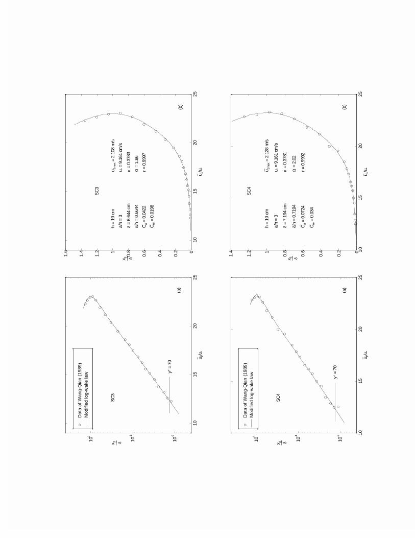
Dat
a of
Wan
g-Q
ian
(198
9)M
odifi
ed lo
g-w
ake
law
1015
2025
10-2
10-1
100
u− 1/u*
x 3 δ___
SC
3
(a)
y+ =
70
1015
2025
0
0.2
0.4
0.6
0.81
1.2
1.4
1.6
u− 1/u *
x 3 δ___
SC
3
h =
10 c
m
a/h
= 3
δ =
6.64
4 cm
δ /h
= 0.
6644
Ca
= 0.
0422
Cm =
0.0
198
u 1m
ax =
2.1
08 m
/s
u * =
9.1
61 c
m/s
κ =
0.37
83
Ω =
1.8
6
r = 0
.999
7
(b)
Dat
a of
Wan
g-Q
ian
(198
9)M
odifi
ed lo
g-w
ake
law
1015
2025
10-2
10-1
100
u− 1/u*
x 3 δ___
SC
4
(a)
y+ =
70
1015
2025
0
0.2
0.4
0.6
0.81
1.2
1.4
u− 1/u *
x 3 δ___
SC
4
h =
10 c
m
a/h
= 3
δ =
7.19
4 cm
δ /h
= 0.
7194
Ca
= 0.
0724
Cm =
0.0
34
u 1m
ax =
2.1
28 m
/s
u * =
9.1
61 c
m/s
κ =
0.37
81
Ω =
2.0
2
r = 0
.999
2
(b)
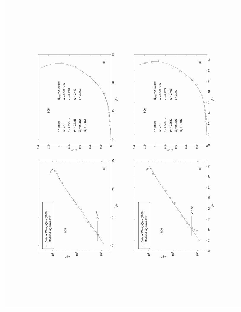
Dat
a of
Wan
g-Q
ian
(198
9)M
odifi
ed lo
g-w
ake
law
1015
2025
10-2
10-1
100
u− 1/u*
x 3 δ___
SC
5
(a)
y+ =
70
1015
2025
0
0.2
0.4
0.6
0.81
1.2
1.4
u− 1/u *
x 3 δ___
SC
5
h =
10 c
m
a/h
= 3
δ =
7.35
5 cm
δ/h
= 0.
7355
Ca
= 0.
1162
Cm =
0.0
651
u 1m
ax =
2.1
49 m
/s
u * =
9.1
61 c
m/s
κ =
0.35
93
Ω =
2.4
49
r = 0
.999
3
(b)
Dat
a of
Wan
g-Q
ian
(198
9)M
odifi
ed lo
g-w
ake
law
810
1214
1618
2022
24
10-2
10-1
100
u− 1/u*
x 3 δ___
SC
6
(a)
y+ =
70
810
1214
1618
2022
240
0.2
0.4
0.6
0.81
1.2
1.4
u− 1/u *
x 3 δ___
SC
6
h =
10 c
m
a/h
= 3
δ =
7.54
2 cm
δ /h
= 0.
7542
Ca
= 0.
1696
Cm =
0.0
937
u 1m
ax =
2.1
73 m
/s
u * =
9.1
61 c
m/s
κ =
0.33
73
Ω =
2.4
62
r = 0
.999
(b)

Dat
a of
Wan
g-Q
ian
(198
9)M
odifi
ed lo
g-w
ake
law
810
1214
1618
2022
24
10-2
10-1
100
u− 1/u*
x 3 δ___
SC
7
(a)
y+ =
70
810
1214
1618
2022
240
0.2
0.4
0.6
0.81
1.2
u− 1/u *
x 3 δ___
SC
7
h =
10 c
m
a/h
= 3
δ =
7.73
4 cm
δ/h
= 0.
7734
Ca
= 0.
21
Cm =
0.1
225
u 1m
ax =
2.1
62 m
/s
u * =
9.1
61 c
m/s
κ =
0.31
73
Ω =
2.1
54
r = 0
.998
5
(b)
Dat
a of
Wan
g-Q
ian
(198
9)M
odifi
ed lo
g-w
ake
law
1214
1618
2022
2426
10-2
10-1
100
u− 1/u*
x 3 δ___
SQ
1
(a)
y+ =
70
1214
1618
2022
2426
0
0.2
0.4
0.6
0.81
1.2
u− 1/u *
x 3 δ___
SQ
1
h =
8 cm
a/h
= 3.
75
δ =
8.17
7 cm
δ /h
= 1.
022
Ca
= 0.
019
Cm =
0.0
053
u 1m
ax =
2.0
84 m
/s
u * =
8.4
05 c
m/s
κ =
0.41
41
Ω =
2.4
22
r = 0
.999
1
(b)
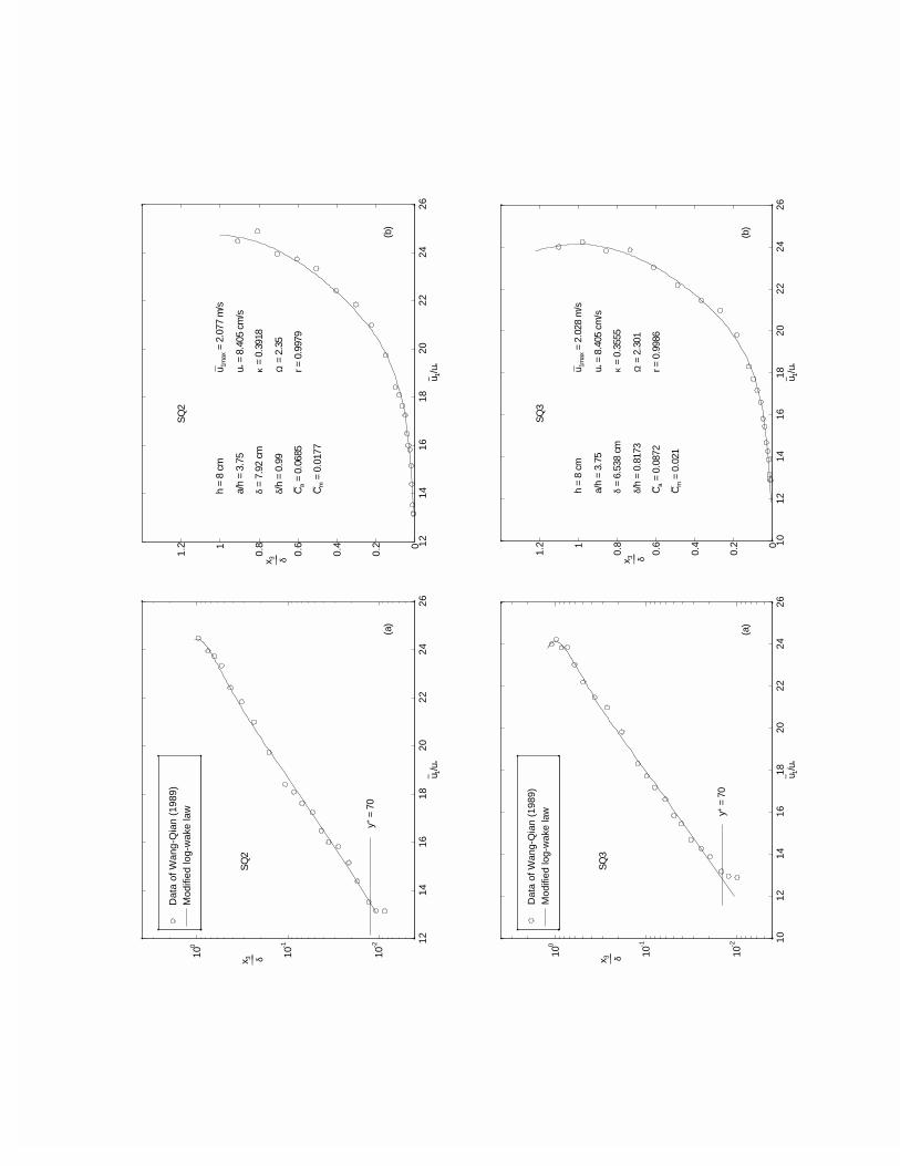
Dat
a of
Wan
g-Q
ian
(198
9)M
odifi
ed lo
g-w
ake
law
1214
1618
2022
2426
10-2
10-1
100
u− 1/u*
x 3 δ___
SQ
2
(a)
y+ =
70
1214
1618
2022
2426
0
0.2
0.4
0.6
0.81
1.2
u− 1/u *
x 3 δ___
SQ
2
h =
8 cm
a/h
= 3.
75
δ =
7.92
cm
δ/h
= 0.
99
Ca
= 0.
0685
Cm =
0.0
177
u 1m
ax =
2.0
77 m
/s
u * =
8.4
05 c
m/s
κ =
0.39
18
Ω =
2.3
5
r = 0
.997
9
(b)
Dat
a of
Wan
g-Q
ian
(198
9)M
odifi
ed lo
g-w
ake
law
1012
1416
1820
2224
26
10-2
10-1
100
u− 1/u*
x 3 δ___
SQ
3
(a)
y+ =
70
1012
1416
1820
2224
260
0.2
0.4
0.6
0.81
1.2
u− 1/u *
x 3 δ___
SQ
3
h =
8 cm
a/h
= 3.
75
δ =
6.53
8 cm
δ /h
= 0.
8173
Ca
= 0.
0872
Cm =
0.0
21
u 1m
ax =
2.0
28 m
/s
u * =
8.4
05 c
m/s
κ =
0.35
55
Ω =
2.3
01
r = 0
.998
6
(b)
Appendix D
ANALYSIS OF COLEMANS
EXPERIMENTAL DATA
Coleman (1986) did experiments in a smooth ßume which is 356 mm wide and
15 m long. During the experiments, the energy slope S was kept to be 0.002 except
the last three runs where S = 0.0022. The ßow depths are about 171 cm. Runs
1, 21, and 32 are clear water ßows. Run2 2-20 are with Þne sands of ds = 0.105
mm; Runs 22-31 are with middle sands of ds = 0.21 mm; and Runs 33-40 are with
coarse sands of ds = 0.42 mm. The temperatures are between 19.5 and 25.3C.
Detailed experimental information can be found in literature (Coleman, 1986). The
measurements of velocity and concentration proÞles are shown in Table D.1. All
velocity proÞle analyses are attached after the table.
173
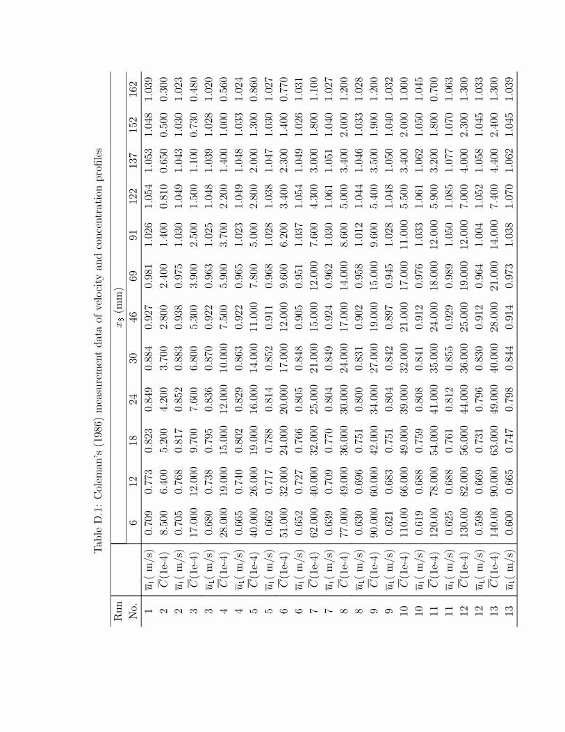
!
"
"#
$%#
""
$&
'"
"
(
%&%
%&&$
%"$
%#
%#
%"&
%
%"
%'#
%'$
%#
%$
")#
'%%
#%%
'"%%
#"%%
$&%%
"%%
"#%%
#%%
%%
%'%
%'%%
%$%%
"(
%&%'
%&
%&
%'"
%$
%$
%&'
%$%
%#
%#$
%$%
%"$
$)#
&%%%
"%%%
&%%
&%%
%%
'$%%
$%%
"'%%
'%%
%%
%&$%
%#%
$(
%%
%&$
%&'
%$
%&%
%""
%$
%"'
%#
%$
%"
%"%
#)#
"%%%
%%%
'%%%
"%%%
%%%%
&'%%
'%%
$&%%
""%%
#%%
%%%
%'%
#(
%'
%&#%
%%"
%"
%$
%""
%'
%"$
%#
%#
%$$
%"#
')#
#%%%%
"%%%
%%%
%%%
#%%%
%%%
&%%
'%%%
"%%
"%%%
$%%
%%
'(
%"
%&&
%&
%#
%'"
%
%
%"
%$
%#&
%$%
%"&
)#
'%%%
$"%%%
"#%%%
"%%%%
&%%%
"%%%
%%
"%%
$#%%
"$%%
#%%
%&&%
(
%'"
%&"&
%&
%%'
%#
%%'
%'
%$&
%'#
%#
%"
%$
&)#
"%%%
#%%%%
$"%%%
"'%%%
"%%%
'%%%
"%%%
&%%
#$%%
$%%%
%%
%%
&(
%$
%&%
%&&%
%%#
%#
%"#
%"
%$%
%
%'
%#%
%"&
)#
&&%%%
#%%%
$%%%
$%%%%
"#%%%
&%%%
#%%%
%%
'%%%
$#%%
"%%%
"%%
(
%$%
%
%&'
%%%
%$
%%"
%'
%"
%##
%#
%$$
%"
)#
%%%%
%%%%
#"%%%
$#%%%
"&%%%
%%%
'%%%
%%
'#%%
$'%%
%%
"%%
(
%"
%$
%&'
%%#
%#"
%&
%#'
%"
%#
%'%
%#%
%$"
%)#
%%%
%%%
#%%%
$%%%
$"%%%
"%%%
&%%%
%%%
''%%
$#%%
"%%%
%%%
%(
%
%
%&'
%%
%#
%"
%&
%$$
%
%"
%'%
%#'
)#
"%%%
&%%%
'#%%%
#%%%
$'%%%
"#%%%
%%%
"%%%
'%%
$"%%
%%
%&%%
(
%"'
%
%&
%"
%''
%"
%
%'%
%'
%&&
%&%
%$
")#
$%%%
"%%%
'%%%
##%%%
$%%%
"'%%%
%%%
"%%%
&%%%
#%%%
"$%%
$%%
"(
%'
%
%&$
%&
%$%
%"
%#
%%#
%'"
%'
%#'
%$$
$)#
#%%%
%%%%
$%%%
#%%%
#%%%%
"%%%
"%%%
#%%%
&#%%
##%%
"#%%
$%%
$(
%%%
%'
%&#&
%&
%##
%#
%&$
%$
%&%
%"
%#'
%$
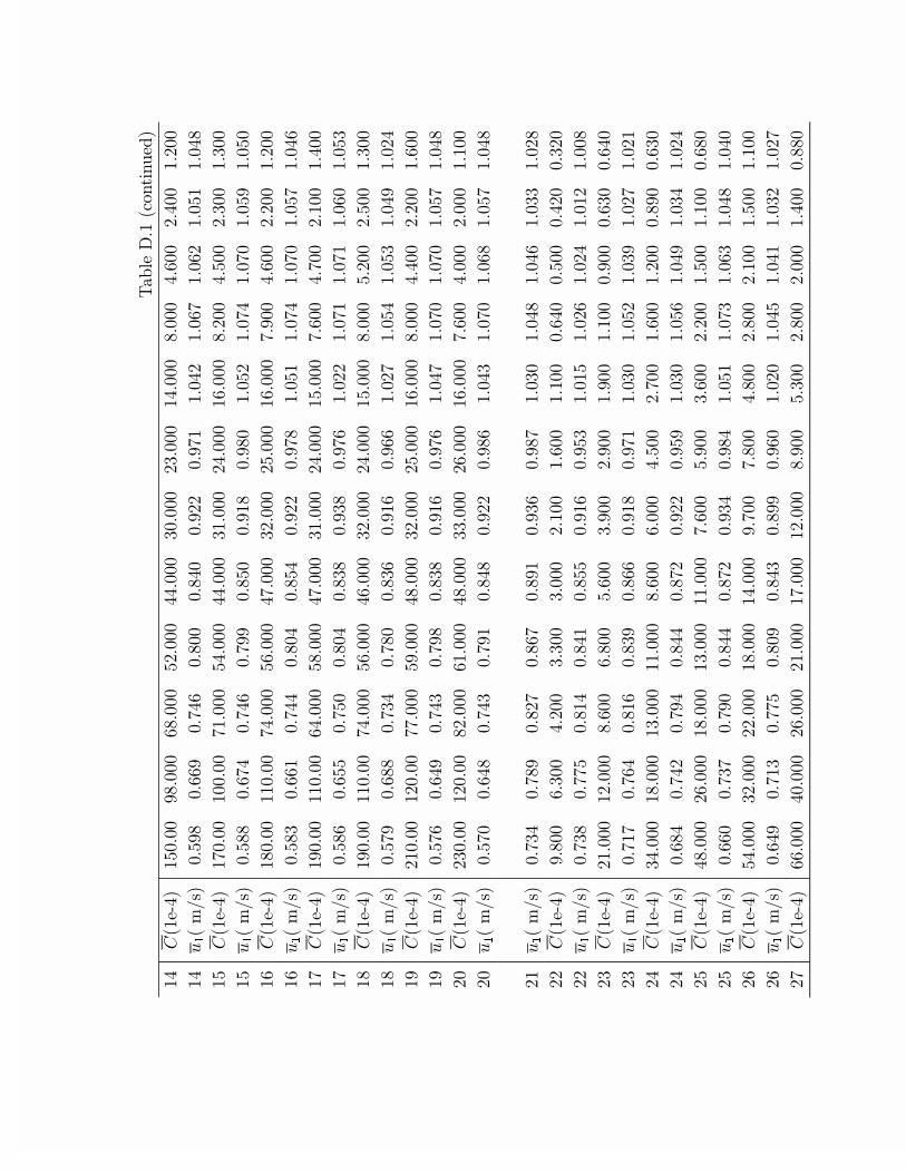
#)#
'%%%
%%%
%%%
'"%%%
##%%%
$%%%%
"$%%%
#%%%
%%%
#%%
"#%%
"%%
#(
%'
%
%&#
%%%
%#%
%""
%&
%#"
%&
%"
%'
%#
')#
&%%%
%%%%
&%%%
'#%%%
##%%%
$%%%
"#%%%
%%%
"%%
#'%%
"$%%
$%%
'(
%'
%&#
%&#
%&
%'%
%
%%
%'"
%&#
%&%
%'
%'%
)#
%%%
%%%
&#%%%
'%%%
#&%%%
$"%%%
"'%%%
%%%
&%%
#%%
""%%
"%%
(
%'$
%
%&##
%%#
%'#
%""
%&
%'
%&#
%&%
%'&
%#
&)#
%%%
%%%
#%%%
'%%%
#&%%%
$%%%
"#%%%
'%%%
&%%
#&%%
"%%
#%%
&(
%'
%''
%&'%
%%#
%$
%$
%&
%""
%&
%&
%%
%'$
)#
%%%
%%%
&#%%%
'%%%
#%%%
$"%%%
"#%%%
'%%%
%%%
'"%%
"'%%
$%%
(
%'&
%
%&$#
%&%
%$
%
%
%"&
%'#
%'$
%#
%"#
)#
"%%%
"%%%
&&%%%
'%%%
#%%%
$"%%%
"'%%%
%%%
%%%
##%%
""%%
%%
(
%'&
%#
%&#$
%&
%$
%
%&
%#&
%&%
%&%
%'&
%#
"%)#
"$%%%
"%%%
"%%%
%%%
#%%%
$$%%%
"%%%
%%%
&%%
#%%%
"%%%
%%
"%(
%'&%
%#
%&#$
%&
%#
%""
%
%#$
%&%
%
%'&
%#
"(
%&$#
%&
%"&
%&
%
%$
%&
%$%
%#
%#
%$$
%"
"")#
%%
$%%
#"%%
$$%%
$%%%
"%%
%%
%%
%#%
%'%%
%#"%
%$"%
""(
%&$
%&&'
%#
%#
%''
%
%'$
%'
%"
%"#
%"
%%
"$)#
"%%%
"%%%
%%
%%
'%%
$%%
"%%
%%
%%
%%%
%$%
%#%
"$(
%&&
%&#
%
%$
%
%
%&
%$%
%'"
%$
%"&
%"
"#)#
$#%%%
%%%
$%%%
%%%
%%
%%%
#'%%
"&%%
%%
"%%
%%
%$%
"#(
%#
%&#"
%&#
%##
%&"
%""
%'
%$%
%'
%#
%$#
%"#
"')#
#%%%
"%%%
%%%
$%%%
%%%
&%%
'%%
$%%
""%%
'%%
%%
%%
"'(
%%
%&$&
%&%
%##
%&"
%$#
%#
%'
%&$
%$
%#
%#%
")#
'#%%%
$"%%%
""%%%
%%%
#%%%
&%%
&%%
#%%
"%%
"%%
'%%
%%
"(
%#
%&$
%&&'
%%
%#$
%
%%
%"%
%#'
%#
%$"
%"&
"&)#
%%%
#%%%%
"%%%
"%%%
&%%%
"%%%
%%
'$%%
"%%
"%%%
#%%
%%
"&(
%"
%&"%
%&&'
%%
%$
%"'
%#
%#"
%&'
%#
%'"
%##
")#
%%%%
#%%%
$%%%
"$%%%
%%%
$%%%
%%
'%%
$$%%
"$%%
&%%
"%%
"(
%$
%&#
%&&
%
%#
%%
%&
%#%
%'
%%
%#$
%##
")#
'%%%
'"%%%
$#%%%
"%%%
"%%%
&%%%
%%%
#%%
$#%%
"%%
%%
%%
"(
%#
%&%
%&&
%"$
%'$
%$%
%
%''
%#
%"
%
%#
$%)#
%%%
'&%%%
$%%%
"%%%
"#%%%
%%%
"%%%
&%%
$&%%
"&%%
%%
%%
$%(
%
%&$
%&&"
%""
%&
%$"
%
%#
%
%$
%&
%&#
$(
%'
%&
%&#$
%&
%"
%
%%
%"
%$
%'
%#
%#"
$)#
"%%%
$%%%
#%%%%
$%%%%
"#%%%
%%%
"%%%
&&%%
#%%
$%%%
"%%%
'%%
$"(
%
%&#
%&
%"
%$
%&
%#
%
%"#
%"'
%"
%%#
$$)#
"&%%
#%%
%%
%%
%'&%
%#$%
%$#%
%"$%
%%
%%
%#%
%"%
$$(
%%
%&#
%&
%$"
%'$
%%$
%#
%"&
%
%#"
%"&
%
$')#
'%%
"#%%
'%%
"%%
%&%
%&%%
%'%
%$"%
%"&%
%"#%
%%
%%
$'(
%&%
%&#'
%&
%"%
%
%%
%'"
%
%#
%'%
%"
%"
$')#
$%%
#%%
""%%
&%%
'%%
%%
%%
%'%
%#"%
%$#%
%$%
%"'%
$'(
%
%&$$
%&
%"
%$
%&
%%
%
%'
%%
%#'
%"
$)#
&%%%
%%
$%%
$%%%
"$%%
&%%
"%%
%%
%%
%#%
%#%%
%$"%
$(
%
%&#%
%%#
%#
%
%#"
%
%''
%%
%%
%
%"
$&)#
%%%
&%%
#&%%
$%%
"%%
""%%
&%%
%%
%%%
%$%
%'#%
%#$%
$&(
%&#
%&"#
%&
%$'
%&
%"%
%'
%'%
%
%&&
%&
%'
$)#
""%%%
%%%
%%%
#%%
#%%%
"&%%
""%%
#%%
%%
%&%
%#%
%''%
$(
%&
%&$'
%%
%#&
%#
%'"
%
%
%
%
%"
$)#
"&%%%
%%%
"%%
#%%
#%%%
$%%%
"$%%
%%
%%%
%%
%%%
%#%
$(
%&&
%&#'
%&
%"
%&
%$
%
%
%
%
%#
%&"
#%)#
"%%%
%%%
#%%
#%%
#"%%
$%%%
"'%%
%%
"%%
%&%
%%%
%%
#%(
%&
%&%
%&"
%$
%&
%$
%'
%
%&
%
%
%%
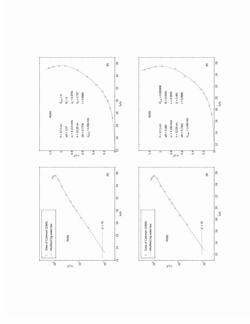
Dat
a of
Col
eman
(19
86)
Mod
ified
log-
wak
e la
w
1214
1618
2022
2426
10-2
10-1
100
u− 1/u*
x 3 δ___
RU
N1
(a)
y+ =
70
1214
1618
2022
2426
0
0.2
0.4
0.6
0.81
1.2
u− 1/u *
x 3 δ___
RU
N1
h =
17.2
cm
a/h
= 2.
07
u * =
4.1
13 c
m/s
δ =
13.2
6 cm
δ /h
= 0.
7709
u 1m
ax =
1.0
54 m
/s
C0.
05 =
0
Ri =
0
κ 0 =
0.3
701
Ω0
= 2.
707
r = 0
.999
6
(b)
Dat
a of
Col
eman
(19
86)
Mod
ified
log-
wak
e la
w
1214
1618
2022
2426
10-2
10-1
100
u− 1/u*
x 3 δ___
RU
N2
(a)
y+ =
70
1214
1618
2022
2426
0
0.2
0.4
0.6
0.81
1.2
u− 1/u *
x 3 δ___
RU
N2
h =
17.1
cm
a/h
= 2.
082
u * =
4.1
08 c
m/s
δ =
12.5
9 cm
δ /h
= 0.
7362
u 1m
ax =
1.0
45 m
/s
C0.
05 =
0.0
0083
6
Ri =
0.9
161
κ =
0.35
09
Ω =
2.4
81
r = 0
.998
8
(b)

Dat
a of
Col
eman
(19
86)
Mod
ified
log-
wak
e la
w
1012
1416
1820
2224
26
10-2
10-1
100
u− 1/u*
x 3 δ___
RU
N3
(a)
y+ =
70
1012
1416
1820
2224
260
0.2
0.4
0.6
0.81
1.2
u− 1/u *
x 3 δ___
RU
N3
h =
17.2
cm
a/h
= 2.
07
u * =
4.1
13 c
m/s
δ =
12.7
cm
δ /h
= 0.
7382
u 1m
ax =
1.0
43 m
/s
C0.
05 =
0.0
0165
7
Ri =
1.8
45
κ =
0.33
37
Ω =
2.7
61
r = 0
.998
(b)
Dat
a of
Col
eman
(19
86)
Mod
ified
log-
wak
e la
w
1012
1416
1820
2224
26
10-2
10-1
100
u− 1/u*
x 3 δ___
RU
N4
(a)
y+ =
70
1012
1416
1820
2224
260
0.2
0.4
0.6
0.81
1.2
u− 1/u *
x 3 δ___
RU
N4
h =
17.1
cm
a/h
= 2.
082
u * =
4.1
08 c
m/s
δ =
12.8
8 cm
δ /h
= 0.
7531
u 1m
ax =
1.0
46 m
/s
C0.
05 =
0.0
0270
6
Ri =
3.1
13
κ =
0.31
85
Ω =
2.7
2
r = 0
.999
1
(b)

Dat
a of
Col
eman
(19
86)
Mod
ified
log-
wak
e la
w
1012
1416
1820
2224
26
10-2
10-1
100
u− 1/u*
x 3 δ___
RU
N5
(a)
y+ =
70
1012
1416
1820
2224
260
0.2
0.4
0.6
0.81
1.2
u− 1/u *
x 3 δ___
RU
N5
h =
17.1
cm
a/h
= 2.
082
u * =
4.1
08 c
m/s
δ =
12.8
6 cm
δ /h
= 0.
7518
u 1m
ax =
1.0
46 m
/s
C0.
05 =
0.0
0387
1
Ri =
4.4
64
κ =
0.32
18
Ω =
3.0
61
r = 0
.998
(b)
Dat
a of
Col
eman
(19
86)
Mod
ified
log-
wak
e la
w
1012
1416
1820
2224
26
10-2
10-1
100
u− 1/u*
x 3 δ___
RU
N6
(a)
y+ =
70
1012
1416
1820
2224
260
0.2
0.4
0.6
0.81
1.2
u− 1/u *
x 3 δ___
RU
N6
h =
17 c
m
a/h
= 2.
094
u * =
4.1
04 c
m/s
δ =
12.7
3 cm
δ /h
= 0.
7488
u 1m
ax =
1.0
52 m
/s
C0.
05 =
0.0
0493
8
Ri =
5.6
61
κ =
0.34
1
Ω =
3.6
97
r = 0
.997
5
(b)

Dat
a of
Col
eman
(19
86)
Mod
ified
log-
wak
e la
w
1012
1416
1820
2224
26
10-2
10-1
100
u− 1/u*
x 3 δ___
RU
N7
(a)
y+ =
70
1012
1416
1820
2224
260
0.2
0.4
0.6
0.81
1.2
u− 1/u *
x 3 δ___
RU
N7
h =
17.1
cm
a/h
= 2.
082
u * =
4.1
08 c
m/s
δ =
12.8
1 cm
δ /h
= 0.
7493
u 1m
ax =
1.0
53 m
/s
C0.
05 =
0.0
0597
2
Ri =
6.8
54
κ =
0.29
48
Ω =
3.1
88
r = 0
.998
(b)
Dat
a of
Col
eman
(19
86)
Mod
ified
log-
wak
e la
w
1012
1416
1820
2224
26
10-2
10-1
100
u− 1/u*
x 3 δ___
RU
N8
(a)
y+ =
70
1012
1416
1820
2224
260
0.2
0.4
0.6
0.81
1.2
u− 1/u *
x 3 δ___
RU
N8
h =
17.1
cm
a/h
= 2.
082
u * =
4.1
08 c
m/s
δ =
13.2
9 cm
δ /h
= 0.
777
u 1m
ax =
1.0
44 m
/s
C0.
05 =
0.0
0730
5
Ri =
8.7
92
κ =
0.29
91
Ω =
3.2
14
r = 0
.998
8
(b)

Dat
a of
Col
eman
(19
86)
Mod
ified
log-
wak
e la
w
810
1214
1618
2022
2426
10-2
10-1
100
u− 1/u*
x 3 δ___
RU
N9
(a)
y+ =
70
810
1214
1618
2022
2426
0
0.2
0.4
0.6
0.81
1.2
u− 1/u *
x 3 δ___
RU
N9
h =
17.2
cm
a/h
= 2.
07
u * =
4.1
13 c
m/s
δ =
13.2
2 cm
δ /h
= 0.
7683
u 1m
ax =
1.0
51 m
/s
C0.
05 =
0.0
0864
3
Ri =
10.
37
κ =
0.28
86
Ω =
3.3
4
r = 0
.997
3
(b)
Dat
a of
Col
eman
(19
86)
Mod
ified
log-
wak
e la
w
810
1214
1618
2022
2426
10-2
10-1
100
u− 1/u*
x 3 δ___
RU
N10
(a)
y+ =
70
810
1214
1618
2022
2426
0
0.2
0.4
0.6
0.81
1.2
u− 1/u *
x 3 δ___
RU
N10
h =
17.1
cm
a/h
= 2.
082
u * =
4.1
08 c
m/s
δ =
13.1
2 cm
δ /h
= 0.
7675
u 1m
ax =
1.0
63 m
/s
C0.
05 =
0.0
1041
Ri =
12.
52
κ =
0.27
03
Ω =
3.2
41
r = 0
.998
8
(b)

Dat
a of
Col
eman
(19
86)
Mod
ified
log-
wak
e la
w
810
1214
1618
2022
2426
28
10-2
10-1
100
u− 1/u*
x 3 δ___
RU
N11
(a)
y+ =
70
810
1214
1618
2022
2426
280
0.2
0.4
0.6
0.81
1.2
u− 1/u *
x 3 δ___
RU
N11
h =
16.9
cm
a/h
= 2.
107
u * =
4.0
99 c
m/s
δ =
13.1
6 cm
δ /h
= 0.
7785
u 1m
ax =
1.0
81 m
/s
C0.
05 =
0.0
1149
Ri =
13.
98
κ =
0.26
12
Ω =
3.4
08
r = 0
.997
9
(b)
Dat
a of
Col
eman
(19
86)
Mod
ified
log-
wak
e la
w
810
1214
1618
2022
2426
10-2
10-1
100
u− 1/u*
x 3 δ___
RU
N12
(a)
y+ =
70
810
1214
1618
2022
2426
0
0.2
0.4
0.6
0.81
1.2
u− 1/u *
x 3 δ___
RU
N12
h =
17.3
cm
a/h
= 2.
058
u * =
4.1
17 c
m/s
δ =
13.7
4 cm
δ /h
= 0.
7941
u 1m
ax =
1.0
49 m
/s
C0.
05 =
0.0
1214
Ri =
15.
33
κ =
0.25
26
Ω =
2.7
9
r = 0
.997
4
(b)

Dat
a of
Col
eman
(19
86)
Mod
ified
log-
wak
e la
w
810
1214
1618
2022
2426
10-2
10-1
100
u− 1/u*
x 3 δ___
RU
N13
(a)
y+ =
70
810
1214
1618
2022
2426
0
0.2
0.4
0.6
0.81
1.2
u− 1/u *
x 3 δ___
RU
N13
h =
17.1
cm
a/h
= 2.
082
u * =
4.1
08 c
m/s
δ =
12.7
4 cm
δ /h
= 0.
7452
u 1m
ax =
1.0
65 m
/s
C0.
05 =
0.0
136
Ri =
15.
77
κ =
0.25
15
Ω =
3.3
73
r = 0
.997
7
(b)
Dat
a of
Col
eman
(19
86)
Mod
ified
log-
wak
e la
w
810
1214
1618
2022
2426
10-2
10-1
100
u− 1/u*
x 3 δ___
RU
N14
(a)
y+ =
70
810
1214
1618
2022
2426
0
0.2
0.4
0.6
0.81
1.2
u− 1/u *
x 3 δ___
RU
N14
h =
17.1
cm
a/h
= 2.
082
u * =
4.1
08 c
m/s
δ =
13.0
9 cm
δ /h
= 0.
7654
u 1m
ax =
1.0
65 m
/s
C0.
05 =
0.0
1442
Ri =
17.
23
κ =
0.24
47
Ω =
3.0
96
r = 0
.997
6
(b)

Dat
a of
Col
eman
(19
86)
Mod
ified
log-
wak
e la
w
68
1012
1416
1820
2224
26
10-2
10-1
100
u− 1/u*
x 3 δ___
RU
N15
(a)
y+ =
70
68
1012
1416
1820
2224
260
0.2
0.4
0.6
0.81
1.2
u− 1/u *
x 3 δ___
RU
N15
h =
17.1
cm
a/h
= 2.
082
u * =
4.1
08 c
m/s
δ =
12.8
2 cm
δ /h
= 0.
7498
u 1m
ax =
1.0
75 m
/s
C0.
05 =
0.0
1632
Ri =
19.
12
κ =
0.23
86
Ω =
3.3
11
r = 0
.998
6
(b)
Dat
a of
Col
eman
(19
86)
Mod
ified
log-
wak
e la
w
68
1012
1416
1820
2224
26
10-2
10-1
100
u− 1/u*
x 3 δ___
RU
N16
(a)
y+ =
70
68
1012
1416
1820
2224
260
0.2
0.4
0.6
0.81
1.2
u− 1/u *
x 3 δ___
RU
N16
h =
17.1
cm
a/h
= 2.
082
u * =
4.1
08 c
m/s
δ =
12.7
6 cm
δ /h
= 0.
7461
u 1m
ax =
1.0
73 m
/s
C0.
05 =
0.0
1742
Ri =
20.
36
κ =
0.22
83
Ω =
3.1
09
r = 0
.997
7
(b)

Dat
a of
Col
eman
(19
86)
Mod
ified
log-
wak
e la
w
68
1012
1416
1820
2224
26
10-2
10-1
100
u− 1/u*
x 3 δ___
RU
N17
(a)
y+ =
70
68
1012
1416
1820
2224
260
0.2
0.4
0.6
0.81
1.2
u− 1/u *
x 3 δ___
RU
N17
h =
17.1
cm
a/h
= 2.
082
u * =
4.1
08 c
m/s
δ =
14.0
2 cm
δ /h
= 0.
8199
u 1m
ax =
1.0
65 m
/s
C0.
05 =
0.0
1751
Ri =
22.
83
κ =
0.22
18
Ω =
2.2
95
r = 0
.996
3
(b)
Dat
a of
Col
eman
(19
86)
Mod
ified
log-
wak
e la
w
68
1012
1416
1820
2224
26
10-2
10-1
100
u− 1/u*
x 3 δ___
RU
N18
(a)
y+ =
70
68
1012
1416
1820
2224
260
0.2
0.4
0.6
0.81
1.2
u− 1/u *
x 3 δ___
RU
N18
h =
17.2
cm
a/h
= 2.
07
u * =
4.1
13 c
m/s
δ =
12.9
1 cm
δ /h
= 0.
7505
u 1m
ax =
1.0
53 m
/s
C0.
05 =
0.0
1817
Ri =
21.
45
κ =
0.24
37
Ω =
3.0
04
r = 0
.998
5
(b)

Dat
a of
Col
eman
(19
86)
Mod
ified
log-
wak
e la
w
68
1012
1416
1820
2224
26
10-2
10-1
100
u− 1/u*
x 3 δ___
RU
N19
(a)
y+ =
70
68
1012
1416
1820
2224
260
0.2
0.4
0.6
0.81
1.2
u− 1/u *
x 3 δ___
RU
N19
h =
17 c
m
a/h
= 2.
094
u * =
4.1
04 c
m/s
δ =
12.9
2 cm
δ /h
= 0.
7599
u 1m
ax =
1.0
72 m
/s
C0.
05 =
0.0
201
Ri =
23.
99
κ =
0.22
8
Ω =
3.2
14
r = 0
.997
9
(b)
Dat
a of
Col
eman
(19
86)
Mod
ified
log-
wak
e la
w
68
1012
1416
1820
2224
26
10-2
10-1
100
u− 1/u*
x 3 δ___
RU
N20
(a)
y+ =
70
68
1012
1416
1820
2224
260
0.2
0.4
0.6
0.81
1.2
u− 1/u *
x 3 δ___
RU
N20
h =
17 c
m
a/h
= 2.
094
u * =
4.1
04 c
m/s
δ =
12.9
1 cm
δ /h
= 0.
7593
u 1m
ax =
1.0
7 m
/s
C0.
05 =
0.0
2177
Ri =
26.
06
κ =
0.21
66
Ω =
2.8
88
r = 0
.997
9
(b)

Dat
a of
Col
eman
(19
86)
Mod
ified
log-
wak
e la
w
1214
1618
2022
2426
10-2
10-1
100
u− 1/u*
x 3 δ___
RU
N21
(a)
y+ =
70
1214
1618
2022
2426
0
0.2
0.4
0.6
0.81
1.2
u− 1/u *
x 3 δ___
RU
N21
h =
16.9
cm
a/h
= 2.
107
u * =
4.0
99 c
m/s
δ =
12.6
1 cm
δ /h
= 0.
7463
u 1m
ax =
1.0
48 m
/s
C0.
05 =
0
Ri =
0
κ 0 =
0.4
003
Ω0
= 2.
598
r = 0
.999
2
(b)
Dat
a of
Col
eman
(19
86)
Mod
ified
log-
wak
e la
w
1416
1820
2224
26
10-2
10-1
100
u− 1/u*
x 3 δ___
RU
N22
(a)
y+ =
70
1416
1820
2224
260
0.2
0.4
0.6
0.81
1.2
u− 1/u *
x 3 δ___
RU
N22
h =
17 c
m
a/h
= 2.
094
u * =
4.1
04 c
m/s
δ =
12.7
2 cm
δ /h
= 0.
7485
u 1m
ax =
1.0
27 m
/s
C0.
05 =
0.0
0095
47
Ri =
1.0
96
κ =
0.50
83
Ω =
3.1
04
r = 0
.997
6
(b)
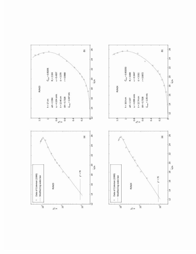
Dat
a of
Col
eman
(19
86)
Mod
ified
log-
wak
e la
w
1214
1618
2022
2426
10-2
10-1
100
u− 1/u*
x 3 δ___
RU
N23
(a)
y+ =
70
1214
1618
2022
2426
0
0.2
0.4
0.6
0.81
1.2
u− 1/u *
x 3 δ___
RU
N23
h =
17 c
m
a/h
= 2.
094
u * =
4.1
04 c
m/s
δ =
12.4
6 cm
δ /h
= 0.
7328
u 1m
ax =
1.0
47 m
/s
C0.
05 =
0.0
0205
Ri =
2.3
24
κ =
0.43
07
Ω =
3.3
78
r = 0
.998
8
(b)
Dat
a of
Col
eman
(19
86)
Mod
ified
log-
wak
e la
w
1214
1618
2022
2426
10-2
10-1
100
u− 1/u*
x 3 δ___
RU
N24
(a)
y+ =
70
1214
1618
2022
2426
0
0.2
0.4
0.6
0.81
1.2
u− 1/u *
x 3 δ___
RU
N24
h =
16.9
cm
a/h
= 2.
107
u * =
4.0
99 c
m/s
δ =
12.7
4 cm
δ /h
= 0.
7538
u 1m
ax =
1.0
5 m
/s
C0.
05 =
0.0
0325
3
Ri =
3.8
08
κ =
0.34
47
Ω =
3.0
11
r = 0
.997
2
(b)

Dat
a of
Col
eman
(19
86)
Mod
ified
log-
wak
e la
w
1012
1416
1820
2224
2628
10-2
10-1
100
u− 1/u*
x 3 δ___
RU
N25
(a)
y+ =
70
1012
1416
1820
2224
2628
0
0.2
0.4
0.6
0.81
1.2
u− 1/u *
x 3 δ___
RU
N25
h =
16.7
cm
a/h
= 2.
132
u * =
4.0
9 cm
/s
δ =
12.4
9 cm
δ /h
= 0.
7481
u 1m
ax =
1.0
69 m
/s
C0.
05 =
0.0
0466
4
Ri =
5.3
77
κ =
0.29
51
Ω =
3.0
88
r = 0
.998
7
(b)
Dat
a of
Col
eman
(19
86)
Mod
ified
log-
wak
e la
w
1012
1416
1820
2224
26
10-2
10-1
100
u− 1/u*
x 3 δ___
RU
N26
(a)
y+ =
70
1012
1416
1820
2224
260
0.2
0.4
0.6
0.81
1.2
u− 1/u *
x 3 δ___
RU
N26
h =
17.1
cm
a/h
= 2.
082
u * =
4.1
08 c
m/s
δ =
13.0
1 cm
δ /h
= 0.
7605
u 1m
ax =
1.0
45 m
/s
C0.
05 =
0.0
0515
6
Ri =
6.1
15
κ =
0.32
4
Ω =
3.2
91
r = 0
.999
1
(b)

Dat
a of
Col
eman
(19
86)
Mod
ified
log-
wak
e la
w
1012
1416
1820
2224
2628
10-2
10-1
100
u− 1/u*
x 3 δ___
RU
N27
(a)
y+ =
70
1012
1416
1820
2224
2628
0
0.2
0.4
0.6
0.81
1.2
u− 1/u *
x 3 δ___
RU
N27
h =
16.8
cm
a/h
= 2.
119
u * =
4.0
95 c
m/s
δ =
12.7
4 cm
δ /h
= 0.
7585
u 1m
ax =
1.0
69 m
/s
C0.
05 =
0.0
0640
2
Ri =
7.5
45
κ =
0.31
95
Ω =
3.7
17
r = 0
.997
4
(b)
Dat
a of
Col
eman
(19
86)
Mod
ified
log-
wak
e la
w
1012
1416
1820
2224
26
10-2
10-1
100
u− 1/u*
x 3 δ___
RU
N28
(a)
y+ =
70
1012
1416
1820
2224
260
0.2
0.4
0.6
0.81
1.2
u− 1/u *
x 3 δ___
RU
N28
h =
17 c
m
a/h
= 2.
094
u * =
4.1
04 c
m/s
δ =
12.9
1 cm
δ /h
= 0.
7596
u 1m
ax =
1.0
63 m
/s
C0.
05 =
0.0
0769
Ri =
9.1
66
κ =
0.30
35
Ω =
3.5
47
r = 0
.998
9
(b)
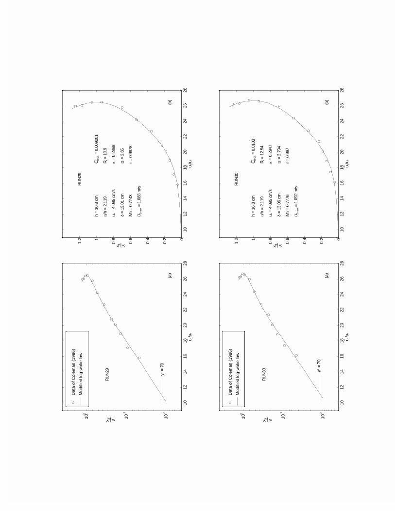
Dat
a of
Col
eman
(19
86)
Mod
ified
log-
wak
e la
w
1012
1416
1820
2224
2628
10-2
10-1
100
u− 1/u*
x 3 δ___
RU
N29
(a)
y+ =
70
1012
1416
1820
2224
2628
0
0.2
0.4
0.6
0.81
1.2
u− 1/u *
x 3 δ___
RU
N29
h =
16.8
cm
a/h
= 2.
119
u * =
4.0
95 c
m/s
δ =
13.0
1 cm
δ /h
= 0.
7743
u 1m
ax =
1.0
83 m
/s
C0.
05 =
0.0
0900
1
Ri =
10.
9
κ =
0.28
68
Ω =
3.6
5
r = 0
.997
8
(b)
Dat
a of
Col
eman
(19
86)
Mod
ified
log-
wak
e la
w
1012
1416
1820
2224
2628
10-2
10-1
100
u− 1/u*
x 3 δ___
RU
N30
(a)
y+ =
70
1012
1416
1820
2224
2628
0
0.2
0.4
0.6
0.81
1.2
u− 1/u *
x 3 δ___
RU
N30
h =
16.8
cm
a/h
= 2.
119
u * =
4.0
95 c
m/s
δ =
13.0
6 cm
δ /h
= 0.
7776
u 1m
ax =
1.0
92 m
/s
C0.
05 =
0.0
103
Ri =
12.
54
κ =
0.29
47
Ω =
3.7
94
r = 0
.997
(b)

Dat
a of
Col
eman
(19
86)
Mod
ified
log-
wak
e la
w
810
1214
1618
2022
2426
10-2
10-1
100
u− 1/u*
x 3 δ___
RU
N31
(a)
y+ =
70
810
1214
1618
2022
2426
0
0.2
0.4
0.6
0.81
1.2
u− 1/u *
x 3 δ___
RU
N31
h =
17.2
cm
a/h
= 2.
07
u * =
4.1
13 c
m/s
δ =
13.2
5 cm
δ /h
= 0.
7703
u 1m
ax =
1.0
6 m
/s
C0.
05 =
0.0
1118
Ri =
13.
69
κ =
0.27
02
Ω =
3.5
34
r = 0
.999
3
(b)
Dat
a of
Col
eman
(19
86)
Mod
ified
log-
wak
e la
w
1214
1618
2022
2426
10-2
10-1
100
u− 1/u*
x 3 δ___
RU
N32
(a)
y+ =
70
1214
1618
2022
2426
0
0.2
0.4
0.6
0.81
1.2
u− 1/u *
x 3 δ___
RU
N32
h =
17.3
cm
a/h
= 2.
058
u * =
4.1
17 c
m/s
δ =
12.8
8 cm
δ /h
= 0.
7443
u 1m
ax =
1.0
25 m
/s
C0.
05 =
0
Ri =
0
κ 0 =
0.4
317
Ω0
= 3.
356
r = 0
.999
7
(b)

Dat
a of
Col
eman
(19
86)
Mod
ified
log-
wak
e la
w
1214
1618
2022
2426
10-2
10-1
100
u− 1/u*
x 3 δ___
RU
N33
(a)
y+ =
70
1214
1618
2022
2426
0
0.2
0.4
0.6
0.81
1.2
u− 1/u *
x 3 δ___
RU
N33
h =
17.4
cm
a/h
= 2.
046
u * =
4.1
21 c
m/s
δ =
13.0
8 cm
δ /h
= 0.
7518
u 1m
ax =
1.0
36 m
/s
C0.
05 =
0.0
0025
4
Ri =
0.2
95
κ =
0.38
88
Ω =
3.0
75
r = 0
.996
4
(b)
Dat
a of
Col
eman
(19
86)
Mod
ified
log-
wak
e la
w
1214
1618
2022
2426
10-2
10-1
100
u− 1/u*
x 3 δ___
RU
N34
(a)
y+ =
70
1214
1618
2022
2426
0
0.2
0.4
0.6
0.81
1.2
u− 1/u *
x 3 δ___
RU
N34
h =
17.2
cm
a/h
= 2.
07
u * =
4.1
13 c
m/s
δ =
12.7
cm
δ /h
= 0.
7384
u 1m
ax =
1.0
44 m
/s
C0.
05 =
0.0
0048
69
Ri =
0.5
595
κ =
0.45
7
Ω =
3.8
25
r = 0
.997
4
(b)
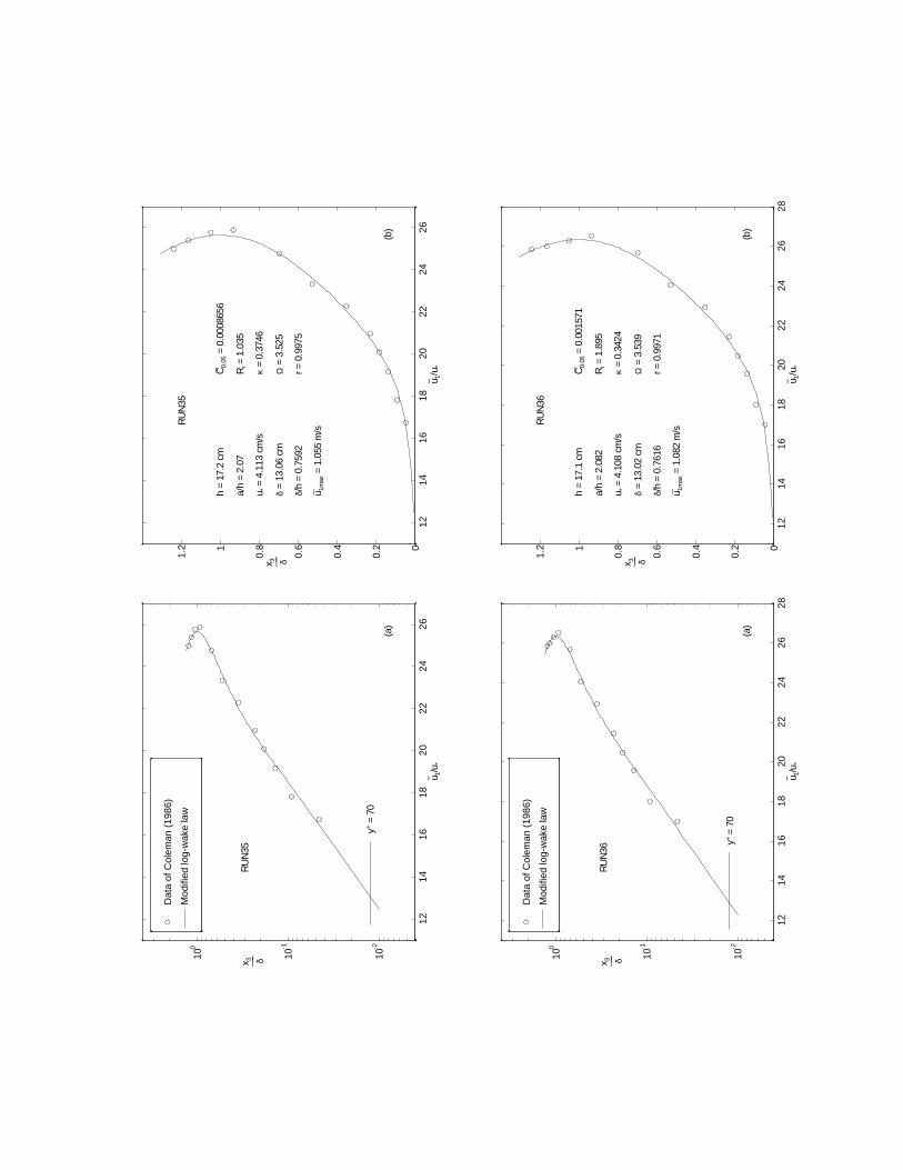
Dat
a of
Col
eman
(19
86)
Mod
ified
log-
wak
e la
w
1214
1618
2022
2426
10-2
10-1
100
u− 1/u*
x 3 δ___
RU
N35
(a)
y+ =
70
1214
1618
2022
2426
0
0.2
0.4
0.6
0.81
1.2
u− 1/u *
x 3 δ___
RU
N35
h =
17.2
cm
a/h
= 2.
07
u * =
4.1
13 c
m/s
δ =
13.0
6 cm
δ /h
= 0.
7592
u 1m
ax =
1.0
55 m
/s
C0.
05 =
0.0
0086
56
Ri =
1.0
35
κ =
0.37
46
Ω =
3.5
25
r = 0
.997
5
(b)
Dat
a of
Col
eman
(19
86)
Mod
ified
log-
wak
e la
w
1214
1618
2022
2426
28
10-2
10-1
100
u− 1/u*
x 3 δ___
RU
N36
(a)
y+ =
70
1214
1618
2022
2426
280
0.2
0.4
0.6
0.81
1.2
u− 1/u *
x 3 δ___
RU
N36
h =
17.1
cm
a/h
= 2.
082
u * =
4.1
08 c
m/s
δ =
13.0
2 cm
δ /h
= 0.
7616
u 1m
ax =
1.0
82 m
/s
C0.
05 =
0.0
0157
1
Ri =
1.8
95
κ =
0.34
24
Ω =
3.5
39
r = 0
.997
1
(b)

Dat
a of
Col
eman
(19
86)
Mod
ified
log-
wak
e la
w
1012
1416
1820
2224
2628
10-2
10-1
100
u− 1/u*
x 3 δ___
RU
N37
(a)
y+ =
70
1012
1416
1820
2224
2628
0
0.2
0.4
0.6
0.81
1.2
u− 1/u *
x 3 δ___
RU
N37
h =
16.7
cm
a/h
= 2.
132
u * =
4.0
9 cm
/s
δ =
12.9
6 cm
δ /h
= 0.
7761
u 1m
ax =
1.0
81 m
/s
C0.
05 =
0.0
0176
4
Ri =
2.1
21
κ =
0.32
76
Ω =
3.7
74
r = 0
.998
1
(b)
Dat
a of
Col
eman
(19
86)
Mod
ified
log-
wak
e la
w
1214
1618
2022
2426
10-2
10-1
100
u− 1/u*
x 3 δ___
RU
N38
(a)
y+ =
70
1214
1618
2022
2426
0
0.2
0.4
0.6
0.81
1.2
u− 1/u *
x 3 δ___
RU
N38
h =
16.7
cm
a/h
= 2.
132
u * =
4.2
9 cm
/s
δ =
13.0
5 cm
δ /h
= 0.
7815
u 1m
ax =
1.1
14 m
/s
C0.
05 =
0.0
0175
1
Ri =
1.9
28
κ =
0.38
5
Ω =
4.2
74
r = 0
.994
8
(b)

Dat
a of
Col
eman
(19
86)
Mod
ified
log-
wak
e la
w
1012
1416
1820
2224
26
10-2
10-1
100
u− 1/u*
x 3 δ___
RU
N39
(a)
y+ =
70
1012
1416
1820
2224
260
0.2
0.4
0.6
0.81
1.2
u− 1/u *
x 3 δ___
RU
N39
h =
17.1
cm
a/h
= 2.
082
u * =
4.3
09 c
m/s
δ =
13.1
5 cm
δ /h
= 0.
7691
u 1m
ax =
1.0
96 m
/s
C0.
05 =
0.0
0247
4
Ri =
2.7
3
κ =
0.35
81
Ω =
3.9
06
r = 0
.998
3
(b)
Dat
a of
Col
eman
(19
86)
Mod
ified
log-
wak
e la
w
1012
1416
1820
2224
2628
10-2
10-1
100
u− 1/u*
x 3 δ___
RU
N40
(a)
y+ =
70
1012
1416
1820
2224
2628
0
0.2
0.4
0.6
0.81
1.2
u− 1/u *
x 3 δ___
RU
N40
h =
17.1
cm
a/h
= 2.
082
u * =
4.1
08 c
m/s
δ =
13.2
1 cm
δ /h
= 0.
7724
u 1m
ax =
1.1
01 m
/s
C0.
05 =
0.0
0237
5
Ri =
2.8
73
κ =
0.31
82
Ω =
4.0
62
r = 0
.995
5
(b)

Appendix E
ANALYSIS OF KIRONOTOS
EXPERIMENTAL DATA
Kironoto (1993), under the guidance of Prof. Walter Graf at Swiss Federal In-
stitute of Technology, Lausanne, Switzerland, did experiments on both uniform and
non-uniform ßows. Only the uniform ßow experimental data are cited here. The
experimental data include both mean velocity proÞles and turbulence intensity dis-
tribution, see next page. All velocity proÞle analyses are attached after the tables.
197
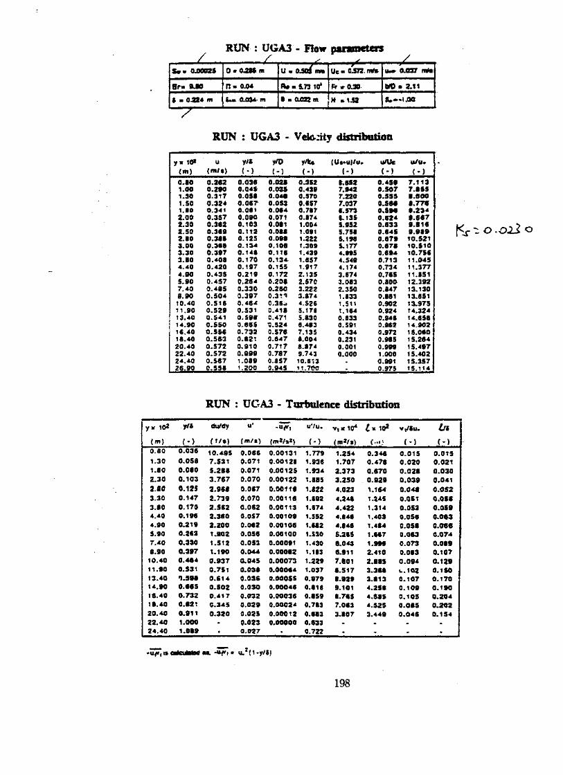
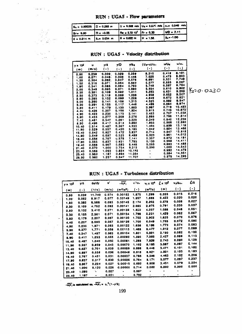
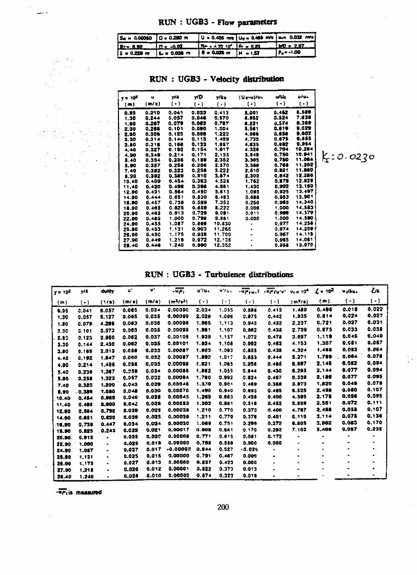
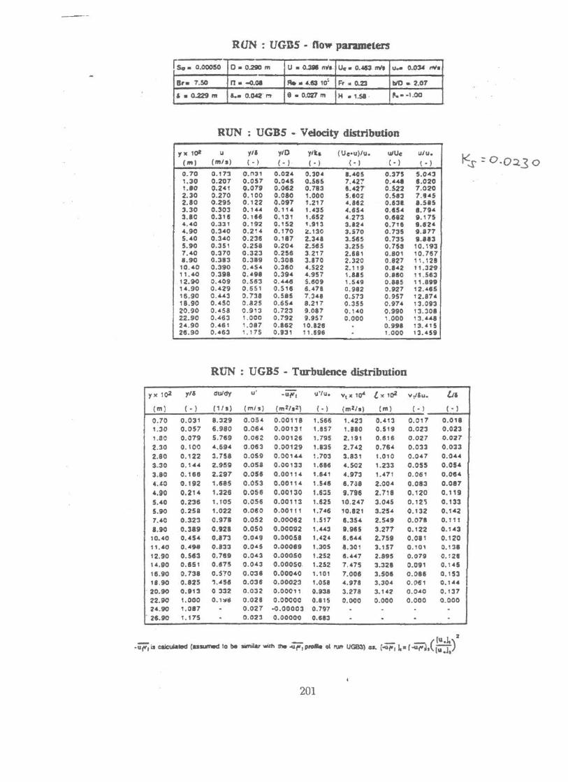
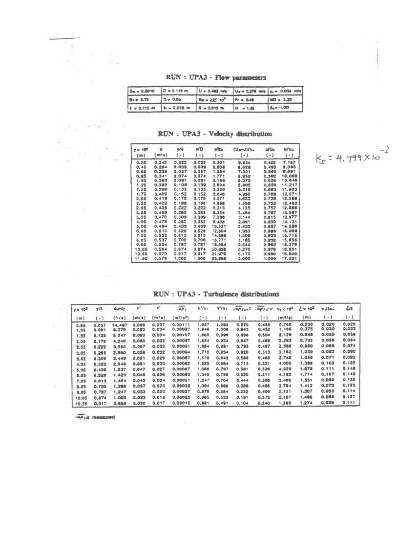
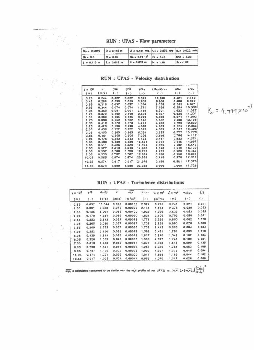
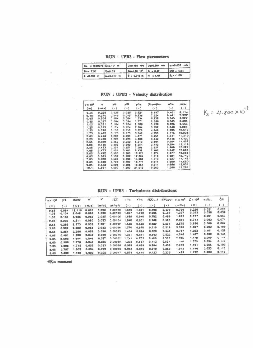
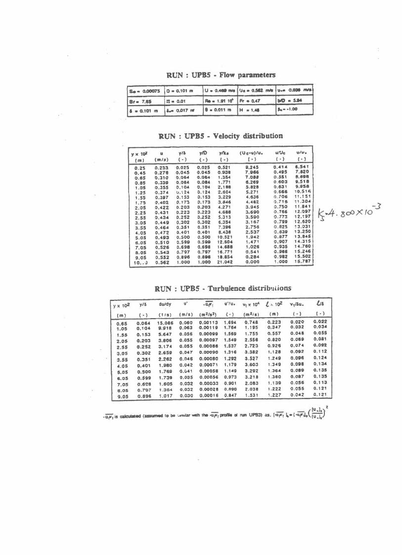
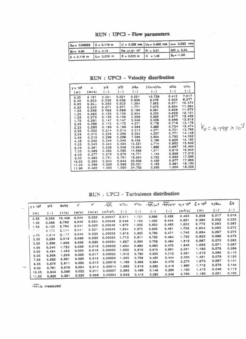
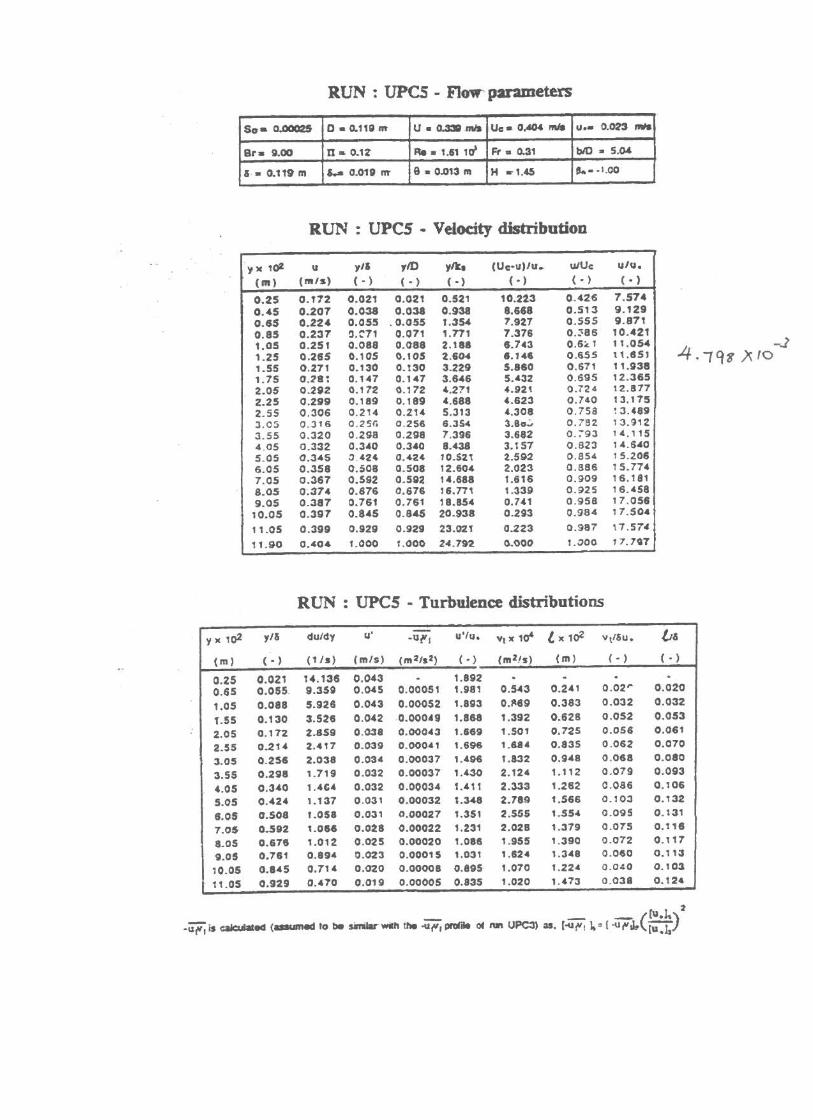
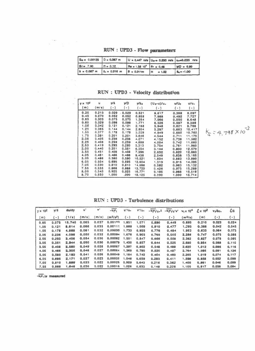
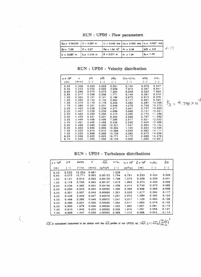

Dat
a of
Kiro
noto
(19
93)
Mod
ified
log-
wak
e la
w
46
810
1214
10-2
10-1
100
u− 1/u*
x 3 δ___
UG
A3
(a)
46
810
1214
0
0.2
0.4
0.6
0.81
1.2
u− 1/u *
x 3 δ___
UG
A3
(ks=
23 m
m)
h =
28.5
cm
a/h
= 2.
11
δ =
21.7
5 cm
δ /h
= 0.
7633
u 1m
ax =
0.5
71 m
/s
u * =
4.1
61 c
m/s
κ 0 =
0.4
06
Ω0
= 1.
637
r = 0
.999
2
(b)
Dat
a of
Kiro
noto
(19
93)
Mod
ified
log-
wak
e la
w
24
68
1012
14
10-2
10-1
100
u− 1/u*
x 3 δ___
UG
A5
(a)
24
68
1012
140
0.2
0.4
0.6
0.81
1.2
u− 1/u *
x 3 δ___
UG
A5
(ks=
23 m
m)
h =
28.5
cm
a/h
= 2.
11
δ =
21.8
1 cm
δ /h
= 0.
7653
u 1m
ax =
0.5
7 m
/s
u * =
4.5
92 c
m/s
κ 0 =
0.4
06
Ω0
= 1.
259
r = 0
.999
5
(b)
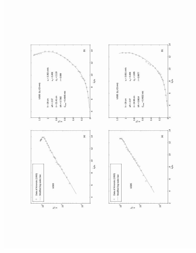
Dat
a of
Kiro
noto
(19
93)
Mod
ified
log-
wak
e la
w
46
810
1214
10-2
10-1
100
u− 1/u*
x 3 δ___
UG
B3
(a)
46
810
1214
0
0.2
0.4
0.6
0.81
1.2
u− 1/u *
x 3 δ___
UG
B3
(ks=
23 m
m)
h =
29 c
m
a/h
= 2.
07
δ =
21.4
1 cm
δ /h
= 0.
7382
u 1m
ax =
0.4
645
m/s
u * =
3.3
52 c
m/s
κ 0 =
0.4
06
Ω0
= 2.
119
r = 0
.999
(b)
Dat
a of
Kiro
noto
(19
93)
Mod
ified
log-
wak
e la
w
24
68
1012
14
10-2
10-1
100
u− 1/u*
x 3 δ___
UG
B5
(a)
24
68
1012
140
0.2
0.4
0.6
0.81
1.2
u− 1/u *
x 3 δ___
UG
B5
(ks=
23 m
m)
h =
29 c
m
a/h
= 2.
07
δ =
24.9
8 cm
δ /h
= 0.
8614
u 1m
ax =
0.4
632
m/s
u * =
3.6
51 c
m/s
κ 0 =
0.4
06
Ω0
= 1.
695
r = 0
.997
7
(b)
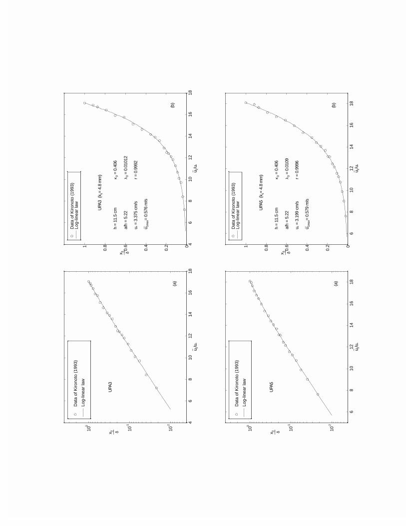
Dat
a of
Kiro
noto
(19
93)
Log-
linea
r la
w
46
810
1214
1618
10-2
10-1
100
u− 1/u*
x 3 δ___
UPA
3
(a)
Dat
a of
Kiro
noto
(19
93)
Log-
linea
r la
w
46
810
1214
1618
0
0.2
0.4
0.6
0.81
u− 1/u *
x 3 δ___
UPA
3 (k
s= 4
.8 m
m)
h =
11.5
cm
a/h
= 5.
22
u * =
3.3
75 c
m/s
u 1m
ax=
0.57
6 m
/s
κ 0 =
0.4
06
λ 0 =
0.0
1012
r = 0
.999
2
(b)
Dat
a of
Kiro
noto
(19
93)
Log-
linea
r la
w
68
1012
1416
18
10-2
10-1
100
u− 1/u*
x 3 δ___
UPA
5
(a)
Dat
a of
Kiro
noto
(19
93)
Log-
linea
r la
w
68
1012
1416
180
0.2
0.4
0.6
0.81
u− 1/u *
x 3 δ___
UPA
5 (k
s= 4
.8 m
m)
h =
11.5
cm
a/h
= 5.
22
u * =
3.1
99 c
m/s
u 1m
ax=
0.57
9 m
/s
κ 0 =
0.4
06
λ 0 =
0.0
109
r = 0
.999
6
(b)

Dat
a of
Kiro
noto
(19
93)
Log-
linea
r la
w
46
810
1214
16
10-2
10-1
100
u− 1/u*
x 3 δ___
UP
B3
(a)
Dat
a of
Kiro
noto
(19
93)
Log-
linea
r la
w
46
810
1214
160
0.2
0.4
0.6
0.81
u− 1/u *
x 3 δ___
UP
B3
(ks=
4.8
mm
)
h =
10.1
cm
a/h
= 5.
94
u * =
3.5
55 c
m/s
u 1m
ax=
0.56
1 m
/s
κ 0 =
0.4
06
λ 0 =
0.0
1153
r = 0
.999
2
(b)
Dat
a of
Kiro
noto
(19
93)
Log-
linea
r la
w
46
810
1214
16
10-2
10-1
100
u− 1/u*
x 3 δ___
UP
B5
(a)
Dat
a of
Kiro
noto
(19
93)
Log-
linea
r la
w
46
810
1214
160
0.2
0.4
0.6
0.81
u− 1/u *
x 3 δ___
UP
B5
(ks=
4.8
mm
)
h =
10.1
cm
a/h
= 5.
94
u * =
3.5
36 c
m/s
u 1m
ax=
0.56
2 m
/s
κ 0 =
0.4
06
λ 0 =
0.0
1077
r = 0
.999
3
(b)
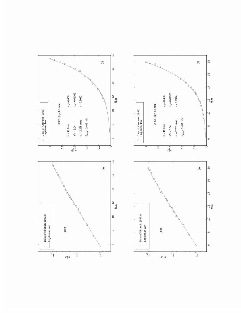
Dat
a of
Kiro
noto
(19
93)
Log-
linea
r la
w
68
1012
1416
18
10-2
10-1
100
u− 1/u*
x 3 δ___
UP
C3
(a)
Dat
a of
Kiro
noto
(19
93)
Log-
linea
r la
w
68
1012
1416
180
0.2
0.4
0.6
0.81
u− 1/u *
x 3 δ___
UP
C3
(ks=
4.8
mm
)
h =
11.9
cm
a/h
= 5.
04
u * =
2.2
98 c
m/s
u 1m
ax=
0.40
2 m
/s
κ 0 =
0.4
06
λ 0 =
0.0
1009
r = 0
.999
2
(b)
Dat
a of
Kiro
noto
(19
93)
Log-
linea
r la
w
68
1012
1416
18
10-2
10-1
100
u− 1/u*
x 3 δ___
UP
C5
(a)
Dat
a of
Kiro
noto
(19
93)
Log-
linea
r la
w
68
1012
1416
180
0.2
0.4
0.6
0.81
u− 1/u *
x 3 δ___
UP
C5
(ks=
4.8
mm
)
h =
11.9
cm
a/h
= 5.
04
u * =
2.2
51 c
m/s
u 1m
ax=
0.40
4 m
/s
κ 0 =
0.4
06
λ 0 =
0.0
1023
r = 0
.999
4
(b)

Dat
a of
Kiro
noto
(19
93)
Log-
linea
r la
w
46
810
1214
16
10-2
10-1
100
u− 1/u*
x 3 δ___
UP
D3
(a)
Dat
a of
Kiro
noto
(19
93)
Log-
linea
r la
w
46
810
1214
160
0.2
0.4
0.6
0.81
u− 1/u *
x 3 δ___
UP
D3
(ks=
4.8
mm
)
h =
8.7
cm
a/h
= 6.
9
u * =
3.3
77 c
m/s
u 1m
ax=
0.55
m/s
κ 0 =
0.4
06
λ 0 =
0.0
1331
r = 0
.999
2
(b)
Dat
a of
Kiro
noto
(19
93)
Log-
linea
r la
w
24
68
1012
1416
10-2
10-1
100
u− 1/u*
x 3 δ___
UP
D5
(a)
Dat
a of
Kiro
noto
(19
93)
Log-
linea
r la
w
24
68
1012
1416
0
0.2
0.4
0.6
0.81
u− 1/u *
x 3 δ___
UP
D5
(ks=
4.8
mm
)
h =
8.7
cm
a/h
= 6.
9
u * =
3.6
72 c
m/s
u 1m
ax=
0.54
5 m
/s
κ 0 =
0.4
06
λ 0 =
0.0
1374
r = 0
.999
6
(b)
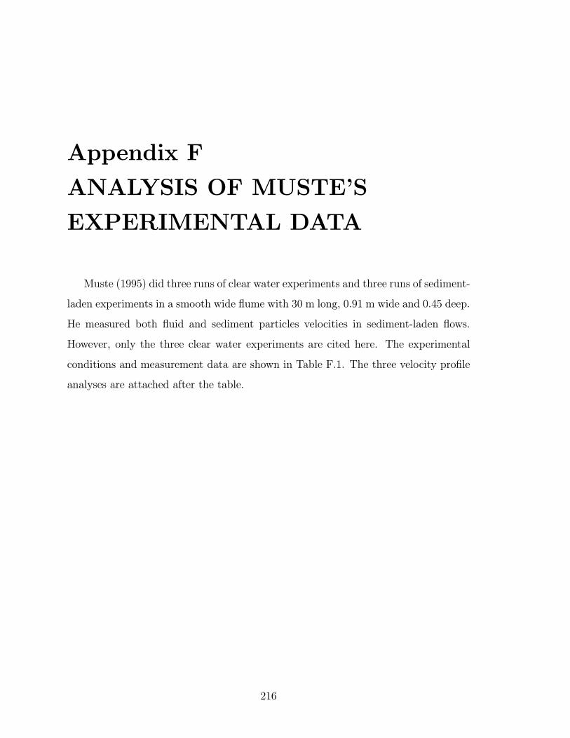
Appendix F
ANALYSIS OF MUSTES
EXPERIMENTAL DATA
Muste (1995) did three runs of clear water experiments and three runs of sediment-
laden experiments in a smooth wide ßume with 30 m long, 0.91 m wide and 0.45 deep.
He measured both ßuid and sediment particles velocities in sediment-laden ßows.
However, only the three clear water experiments are cited here. The experimental
conditions and measurement data are shown in Table F.1. The three velocity proÞle
analyses are attached after the table.
216
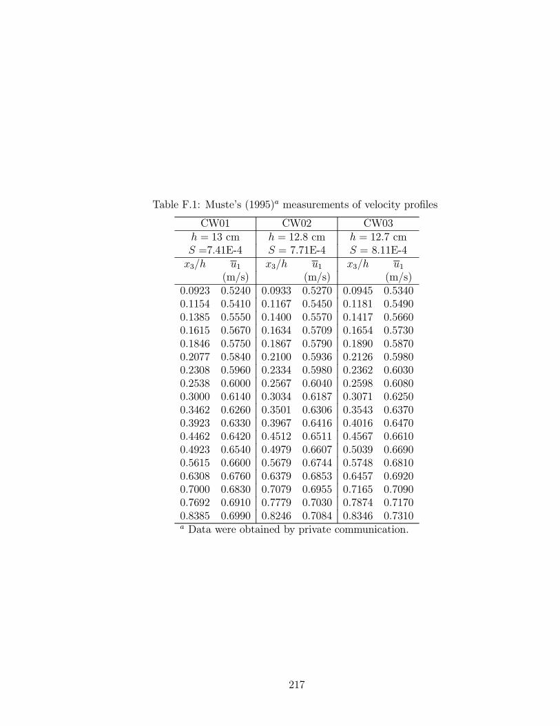
Table F.1: Mustes (1995)a measurements of velocity proÞles
CW01 CW02 CW03h = 13 cm h = 12.8 cm h = 12.7 cmS =7.41E-4 S = 7.71E-4 S = 8.11E-4x3/h u1 x3/h u1 x3/h u1
(m/s) (m/s) (m/s)0.0923 0.5240 0.0933 0.5270 0.0945 0.53400.1154 0.5410 0.1167 0.5450 0.1181 0.54900.1385 0.5550 0.1400 0.5570 0.1417 0.56600.1615 0.5670 0.1634 0.5709 0.1654 0.57300.1846 0.5750 0.1867 0.5790 0.1890 0.58700.2077 0.5840 0.2100 0.5936 0.2126 0.59800.2308 0.5960 0.2334 0.5980 0.2362 0.60300.2538 0.6000 0.2567 0.6040 0.2598 0.60800.3000 0.6140 0.3034 0.6187 0.3071 0.62500.3462 0.6260 0.3501 0.6306 0.3543 0.63700.3923 0.6330 0.3967 0.6416 0.4016 0.64700.4462 0.6420 0.4512 0.6511 0.4567 0.66100.4923 0.6540 0.4979 0.6607 0.5039 0.66900.5615 0.6600 0.5679 0.6744 0.5748 0.68100.6308 0.6760 0.6379 0.6853 0.6457 0.69200.7000 0.6830 0.7079 0.6955 0.7165 0.70900.7692 0.6910 0.7779 0.7030 0.7874 0.71700.8385 0.6990 0.8246 0.7084 0.8346 0.7310a Data were obtained by private communication.
217
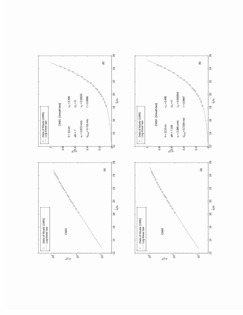
Dat
a of
Mus
te (
1995
)Lo
g-lin
ear
law
1214
1618
2022
2426
10-2
10-1
100
u− 1/u*
x 3 h___
CW
01
(a)
Dat
a of
Mus
te (
1995
)Lo
g-lin
ear
law
1214
1618
2022
2426
0
0.2
0.4
0.6
0.81
u− 1/u *
x 3 h___
CW
01 (
Sm
ooth
bed
)
h =
13 c
m
a/h
= 7
u * =
2.8
73 c
m/s
u 1m
ax=
0.71
5 m
/s
κ 0 =
0.4
06
Ω0
= 0
λ 0 =
0.0
0531
r = 0
.999
5
(b)
Dat
a of
Mus
te (
1995
)Lo
g-lin
ear
law
1214
1618
2022
2426
10-2
10-1
100
u− 1/u*
x 3 h___
CW
02
(a)
Dat
a of
Mus
te (
1995
)Lo
g-lin
ear
law
1214
1618
2022
2426
0
0.2
0.4
0.6
0.81
u− 1/u *
x 3 h___
CW
02 (
Sm
ooth
bed
)
h =
12.8
cm
a/h
= 7.
109
u * =
2.8
85 c
m/s
u 1m
ax=
0.72
94 m
/s
κ 0 =
0.4
06
Ω0
= 0
λ 0 =
0.0
0584
4
r = 0
.999
7
(b)
Dat
a of
Mus
te (
1995
)Lo
g-lin
ear
law
1520
2530
10-2
10-1
100
u− 1/u*
x 3 h___
CW
03
(a)
Dat
a of
Mus
te (
1995
)Lo
g-lin
ear
law
1520
2530
0
0.2
0.4
0.6
0.81
u− 1/u *
x 3 h___
CW
03 (
Sm
ooth
bed
)
h =
12.7
cm
a/h
= 7.
165
u * =
2.4
85 c
m/s
u 1m
ax=
0.75
03 m
/s
κ 0 =
0.4
06
Ω0
= 0
λ 0 =
0.0
0614
3
r = 0
.999
3
(b)
Appendix G
ANALYSIS OF McQUIVEYS
EXPERIMENTAL DATA
McQuivey (1971) collected a lot of experimental data. The data in a 20 centimeter-
wide ßume with a rigid boundary are cited and analyzed here, see attached table and
Þgures.
220
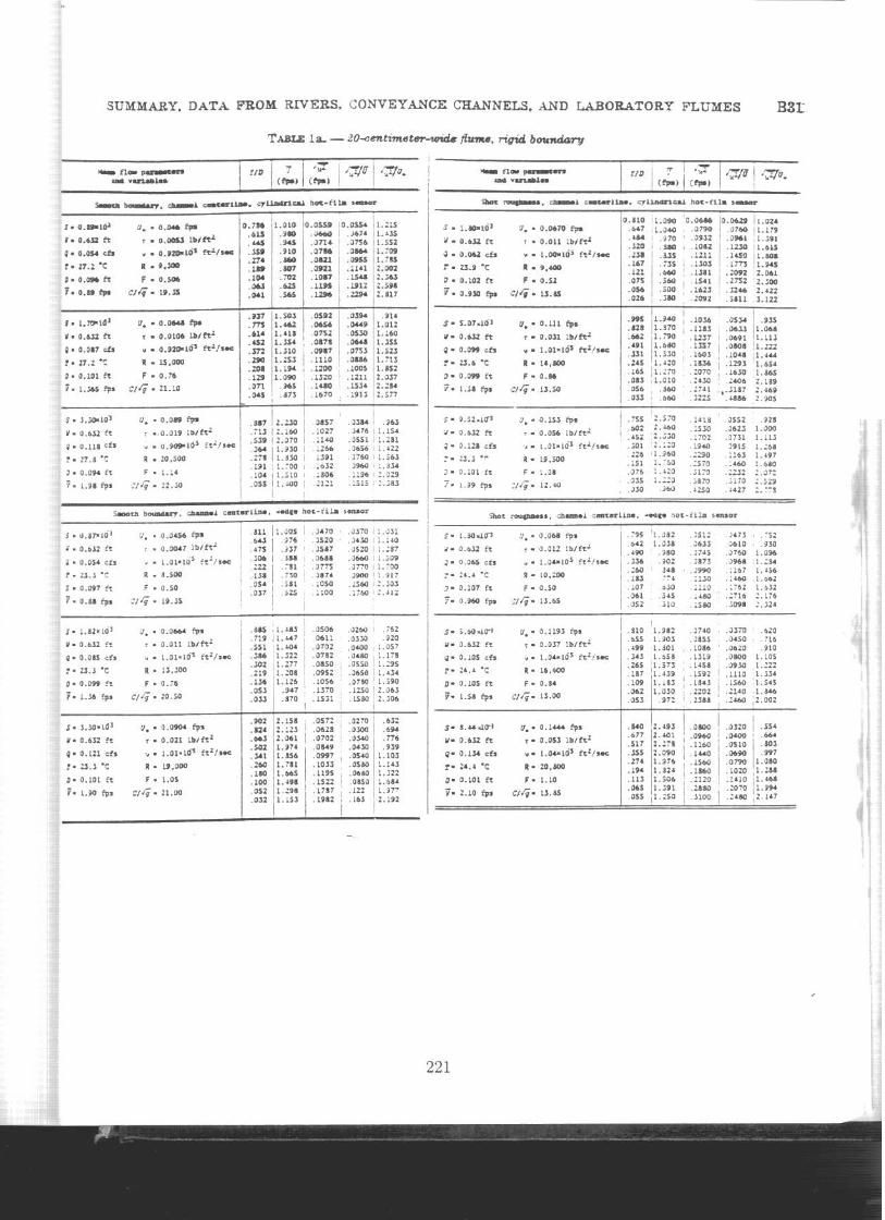

Dat
a of
McQ
uive
y (1
971)
Log-
linea
r la
w
46
810
1214
16
10-2
10-1
100
u− 1/u*
x 3 h___
RU
N 1
(a)
Dat
a of
McQ
uive
y (1
971)
Log-
linea
r la
w
46
810
1214
160
0.2
0.4
0.6
0.81
u− 1/u *
x 3 h___
RU
N 1
(Sm
ooth
bed
)
h =
2.92
6 cm
a/h
= 6.
583
u 1m
ax=
0.31
77 m
/s
u * =
2.0
79 c
m/s
κ 0 =
0.4
06
λ 0 =
0.0
0715
4
r = 0
.999
3
(b)
Dat
a of
McQ
uive
y (1
971)
Log-
linea
r la
w
68
1012
1416
18
10-2
10-1
100
u− 1/u*
x 3 h___
RU
N 2
(a)
Dat
a of
McQ
uive
y (1
971)
Log-
linea
r la
w
68
1012
1416
180
0.2
0.4
0.6
0.81
u− 1/u *
x 3 h___
RU
N 2
(Sm
ooth
bed
)
h =
3.07
8 cm
a/h
= 6.
257
u 1m
ax=
0.46
24 m
/s
u * =
2.5
69 c
m/s
κ 0 =
0.4
06
λ 0 =
0.0
0765
8
r = 0
.999
9
(b)
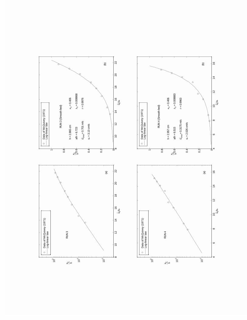
Dat
a of
McQ
uive
y (1
971)
Log-
linea
r la
w
810
1214
1618
2022
10-2
10-1
100
u− 1/u*
x 3 h___
RU
N 3
(a)
Dat
a of
McQ
uive
y (1
971)
Log-
linea
r la
w
810
1214
1618
2022
0
0.2
0.4
0.6
0.81
u− 1/u *
x 3 h___
RU
N 3
(Sm
ooth
bed
)
h =
2.86
5 cm
a/h
= 6.
723
u 1m
ax=
0.70
1 m
/s
u * =
3.1
3 cm
/s
κ 0 =
0.4
06
λ 0 =
0.0
0886
8
r = 0
.997
6
(b)
Dat
a of
McQ
uive
y (1
971)
Log-
linea
r la
w
46
810
1214
16
10-2
10-1
100
u− 1/u*
x 3 h___
RU
N 4
(a)
Dat
a of
McQ
uive
y (1
971)
Log-
linea
r la
w
46
810
1214
160
0.2
0.4
0.6
0.81
u− 1/u *
x 3 h___
RU
N 4
(Sm
ooth
bed
)
h =
2.95
7 cm
a/h
= 6.
515
u 1m
ax=
0.31
75 m
/s
u * =
2.0
26 c
m/s
κ 0 =
0.4
06
λ 0 =
0.0
0888
3
r = 0
.996
3
(b)
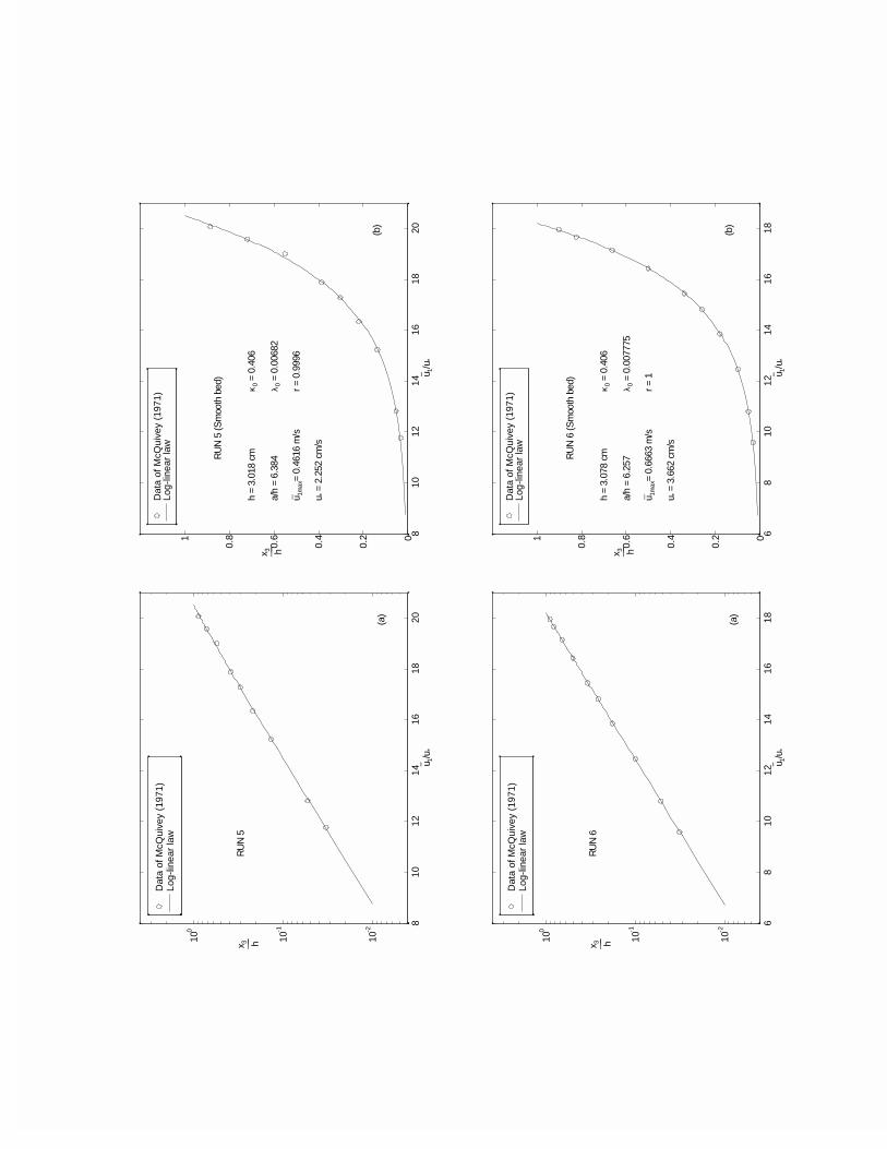
Dat
a of
McQ
uive
y (1
971)
Log-
linea
r la
w
810
1214
1618
20
10-2
10-1
100
u− 1/u*
x 3 h___
RU
N 5
(a)
Dat
a of
McQ
uive
y (1
971)
Log-
linea
r la
w
810
1214
1618
200
0.2
0.4
0.6
0.81
u− 1/u *
x 3 h___
RU
N 5
(Sm
ooth
bed
)
h =
3.01
8 cm
a/h
= 6.
384
u 1m
ax=
0.46
16 m
/s
u * =
2.2
52 c
m/s
κ 0 =
0.4
06
λ 0 =
0.0
0682
r = 0
.999
6
(b)
Dat
a of
McQ
uive
y (1
971)
Log-
linea
r la
w
68
1012
1416
18
10-2
10-1
100
u− 1/u*
x 3 h___
RU
N 6
(a)
Dat
a of
McQ
uive
y (1
971)
Log-
linea
r la
w
68
1012
1416
180
0.2
0.4
0.6
0.81
u− 1/u *
x 3 h___
RU
N 6
(Sm
ooth
bed
)
h =
3.07
8 cm
a/h
= 6.
257
u 1m
ax=
0.66
63 m
/s
u * =
3.6
62 c
m/s
κ 0 =
0.4
06
λ 0 =
0.0
0777
5
r = 1
(b)

Dat
a of
McQ
uive
y (1
971)
Log-
linea
r la
w
24
68
1012
14
10-2
10-1
100
u− 1/u*
x 3 h___
RU
N 7
(a)
Dat
a of
McQ
uive
y (1
971)
Log-
linea
r la
w
24
68
1012
140
0.2
0.4
0.6
0.81
u− 1/u *
x 3 h___
RU
N 7
(Rou
gh b
ed)
h =
3.10
9 cm
a/h
= 6.
196
u 1m
ax=
0.35
09 m
/s
u * =
2.4
24 c
m/s
κ 0 =
0.4
06
λ 0 =
0.0
1633
r = 0
.998
6
(b)
Dat
a of
McQ
uive
y (1
971)
Log-
linea
r la
w
02
46
810
1214
10-2
10-1
100
u− 1/u*
x 3 h___
RU
N 8
(a)
Dat
a of
McQ
uive
y (1
971)
Log-
linea
r la
w
02
46
810
1214
0
0.2
0.4
0.6
0.81
u− 1/u *
x 3 h___
RU
N 8
(Rou
gh b
ed)
h =
3.01
8 cm
a/h
= 6.
384
u 1m
ax=
0.59
11 m
/s
u * =
4.7
16 c
m/s
κ 0 =
0.4
06
λ 0 =
0.0
1481
r = 1
(b)

Dat
a of
McQ
uive
y (1
971)
Log-
linea
r la
w
24
68
1012
14
10-2
10-1
100
u− 1/u*
x 3 h___
RU
N 9
(a)
Dat
a of
McQ
uive
y (1
971)
Log-
linea
r la
w
24
68
1012
140
0.2
0.4
0.6
0.81
u− 1/u *
x 3 h___
RU
N 9
(Rou
gh b
ed)
h =
3.07
8 cm
a/h
= 6.
257
u 1m
ax=
0.82
84 m
/s
u * =
6.1
98 c
m/s
κ 0 =
0.4
06
λ 0 =
0.0
1394
r = 0
.999
9
(b)
Dat
a of
McQ
uive
y (1
971)
Log-
linea
r la
w
24
68
1012
14
10-2
10-1
100
u− 1/u*
x 3 h___
RU
N 1
0
(a)
Dat
a of
McQ
uive
y (1
971)
Log-
linea
r la
w
24
68
1012
140
0.2
0.4
0.6
0.81
u− 1/u *
x 3 h___
RU
N 1
0 (R
ough
bed
)
h =
3.26
1 cm
a/h
= 5.
907
u 1m
ax=
0.34
63 m
/s
u * =
2.5
79 c
m/s
κ 0 =
0.4
06
λ 0 =
0.0
1474
r = 0
.998
9
(b)

Dat
a of
McQ
uive
y (1
971)
Log-
linea
r la
w
24
68
1012
14
10-2
10-1
100
u− 1/u*
x 3 h___
RU
N 1
1
(a)
Dat
a of
McQ
uive
y (1
971)
Log-
linea
r la
w
24
68
1012
140
0.2
0.4
0.6
0.81
u− 1/u *
x 3 h___
RU
N 1
1 (R
ough
bed
)
h =
3.2
cm
a/h
= 6.
019
u 1m
ax=
0.63
06 m
/s
u * =
4.5
53 c
m/s
κ 0 =
0.4
06
λ 0 =
0.0
1384
r = 0
.998
8
(b)
Dat
a of
McQ
uive
y (1
971)
Log-
linea
r la
w
24
68
1012
1416
10-2
10-1
100
u− 1/u*
x 3 h___
RU
N 1
2
(a)
Dat
a of
McQ
uive
y (1
971)
Log-
linea
r la
w
24
68
1012
1416
0
0.2
0.4
0.6
0.81
u− 1/u *
x 3 h___
RU
N 1
2 (R
ough
bed
)
h =
3.07
8 cm
a/h
= 6.
257
u 1m
ax=
0.78
72 m
/s
u * =
5.2
74 c
m/s
κ 0 =
0.4
06
λ 0 =
0.0
1277
r = 0
.999
1
(b)
Appendix H
ANALYSIS OF GUY, SIMONS
AND RICHARDSONS
EXPERIMENTAL DATA
Eight velocity proÞle measurements over plane beds by Guy, Simons and Richard-
son (1966) are cited. The ßow conditions and measurement data are listed in Table
H.1. The analyses of velocity proÞle are attached after the table.
228
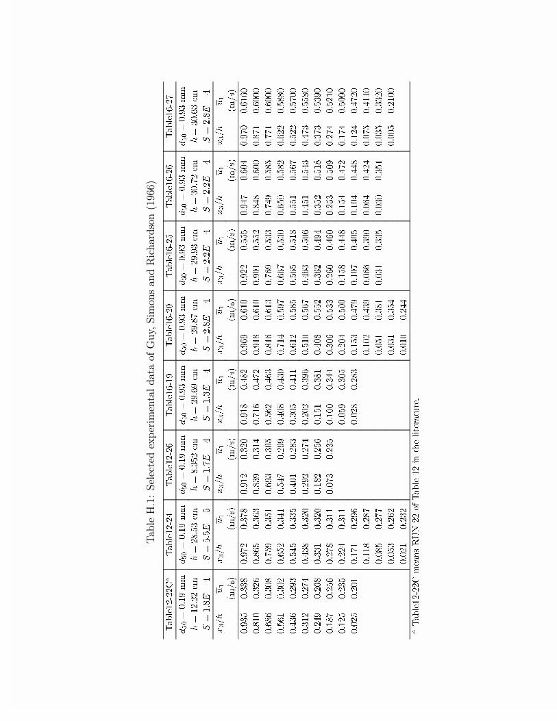
Wdeoh45055Fd
Wdeoh45057
Wdeoh45059
Wdeoh4904<
Wdeoh49053
Wdeoh49058
Wdeoh49059
Wdeoh4905:
g83@
3=4<pp
g83@
3=4<pp
g83@
3=4<pp
g83@
3=<6pp
g83@
3=<6pp
g83@
3=<6pp
g83@
3=<6pp
g83@
3=<6pp
k@
45=55fp
k@
5;=86fp
k@
;=685fp
k@
5<=9<fp
k@
5<=;:fp
k@
5<=<6fp
k@
63=:5fp
k@
63=96fp
V@
4=;H7
V@
8=8H8
V@
4=:H7
V@
4=6H7
V@
5=;H7
V@
5=5H7
V@
5=5H7
V@
5=;H7
6@k
x4
6@k
x4
6@k
x4
6@k
x4
6@k
x4
6@k
x4
6@k
x4
6@k
x4
+p2v,
+p2v,
+p2v,
+p2v,
+p2v,
+p2v,
+p2v,
+p2v,
31<68
3166;
31<:5
316:;
31<45
31653
31<4;
317;5
31<9<
31943
31<55
31888
31<7:
31937
31<:3
319493
31;43
31659
31;98
31696
31;6<
31647
31:49
317:5
31<4;
31943
31<34
31885
31;7;
31933
31;:4
319333
319;9
3163;
31:8<
31684
319<6
31638
31895
31796
31;49
31946
31:9<
31866
31:7<
318;8
31::4
319333
31894
31635
31985
31674
3187:
315<<
3173;
31763
31:47
318<:
3199:
31863
31983
318;5
31955
318;;3
31769
315<6
31878
31668
31734
315;6
31638
31744
31945
318;8
31898
3184;
31884
3189:
31855
318:33
31645
315:7
3176;
31653
315<5
315:7
31535
316<9
31843
3189:
31796
31839
31784
31876
317:6
3188;3
3157<
3159;
31664
31653
314;5
31589
31484
316;4
3173;
31885
31695
317<7
31685
3184;
316:6
3186<3
314;:
31589
315:;
31644
313:6
31568
31433
31677
31639
31866
31593
31793
31586
3183<
315:7
318543
31458
31568
31557
31644
3138<
31638
31537
31833
3148;
3177;
31487
317:5
314:7
3183<3
31358
31534
314:4
315<9
3135;
315;6
31486
317:<
3143:
31738
31437
3177;
31457
317:53
3144;
315;:
31435
3176<
31399
316<3
31397
31757
313:8
317443
313;8
315::
31384
316;4
31364
31668
31363
31684
31368
316653
31386
31595
31364
31687
31338
315433
31354
31565
31343
31577
dWdeoh45055F
phdqvUXQ
55riWdeoh
45lq
wkholwhudwxuh1
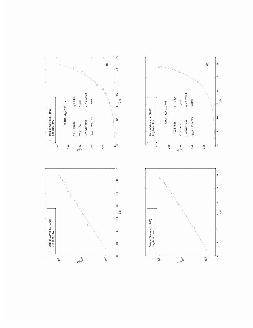
Dat
a of
Guy
et a
l. (1
966)
Log-
linea
r la
w
810
1214
1618
2022
10-2
10-1
100
u− 1/u *
x 3 δ___
Dat
a of
Guy
et a
l. (1
966)
Log-
linea
r la
w
810
1214
1618
2022
0
0.2
0.4
0.6
0.81
u− 1/u *
x 3 δ___
RU
N19
(d 5
0= 0
.93
mm
)
h =
29.6
9 cm
a/h
= 8.
214
u * =
2.3
44 c
m/s
u 1m
ax=
0.49
25 m
/s
κ 0 =
0.4
06
Ω0 =
0
λ 0 =
0.0
0665
6
r = 0
.994
1
(b)
Dat
a of
Guy
et a
l. (1
966)
Log-
linea
r la
w
68
1012
1416
18
10-2
10-1
100
u− 1/u *
x 3 δ___
Dat
a of
Guy
et a
l. (1
966)
Log-
linea
r la
w
68
1012
1416
180
0.2
0.4
0.6
0.81
u− 1/u *
x 3 δ___
RU
N20
(d 5
0= 0
.93
mm
)
h =
29.8
7 cm
a/h
= 8.
163
u * =
3.4
77 c
m/s
u 1m
ax=
0.61
67 m
/s
κ 0 =
0.4
06
Ω0 =
0
λ 0 =
0.0
0558
8
r = 0
.999
(b)

Dat
a of
Guy
et a
l. (1
966)
Log-
linea
r la
w
1820
2224
2628
3032
3436
38
10-2
10-1
100
u− 1/u *
x 3 δ___
Dat
a of
Guy
et a
l. (1
966)
Log-
linea
r la
w
1820
2224
2628
3032
3436
380
0.2
0.4
0.6
0.81
u− 1/u *
x 3 δ___
RU
N22
C (
d 50=
0.1
9 m
m)
h =
12.2
2 cm
a/h
= 19
.95
u * =
0.9
02 c
m/s
u 1m
ax=
0.34
19 m
/s
κ 0 =
0.4
06
Ω0 =
0
λ 0 =
0.0
0647
6
r = 0
.996
1
(b)
Dat
a of
Guy
et a
l. (1
966)
Log-
linea
r la
w
2224
2628
3032
3436
10-2
10-1
100
u− 1/u *
x 3 δ___
Dat
a of
Guy
et a
l. (1
966)
Log-
linea
r la
w
2224
2628
3032
3436
0
0.2
0.4
0.6
0.81
u− 1/u *
x 3 δ___
RU
N24
(d 5
0= 0
.19
mm
)
h =
28.5
3 cm
a/h
= 8.
547
u * =
1.0
36 c
m/s
u 1m
ax=
0.37
06 m
/s
κ 0 =
0.4
06
Ω0 =
0
λ 0 =
0.0
0470
1
r = 0
.992
5
(b)

Dat
a of
Guy
et a
l. (1
966)
Log-
linea
r la
w
1012
1416
1820
2224
10-2
10-1
100
u− 1/u *
x 3 δ___
Dat
a of
Guy
et a
l. (1
966)
Log-
linea
r la
w
1012
1416
1820
2224
0
0.2
0.4
0.6
0.81
u− 1/u *
x 3 δ___
RU
N25
(d 5
0= 0
.93
mm
)
h =
29.9
3 cm
a/h
= 8.
147
u * =
2.4
41 c
m/s
u 1m
ax=
0.55
76 m
/s
κ 0 =
0.4
06
Ω0 =
0
λ 0 =
0.0
0555
4
r = 0
.996
8
(b)
Dat
a of
Guy
et a
l. (1
966)
Log-
linea
r la
w
1820
2224
2628
3032
34
10-2
10-1
100
u− 1/u *
x 3 δ___
Dat
a of
Guy
et a
l. (1
966)
Log-
linea
r la
w
1820
2224
2628
3032
340
0.2
0.4
0.6
0.81
u− 1/u *
x 3 δ___
RU
N26
(d 5
0= 0
.19
mm
)
h =
8.35
2 cm
a/h
= 29
.2
u * =
0.9
461
cm/s
u 1m
ax=
0.32
43 m
/s
κ 0 =
0.4
06
Ω0 =
0
λ 0 =
0.0
0496
1
r = 0
.998
3
(b)
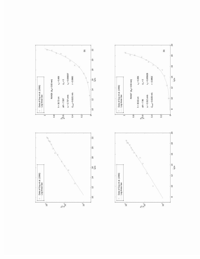
Dat
a of
Guy
et a
l. (1
966)
Log-
linea
r la
w
1012
1416
1820
22
10-2
10-1
100
u− 1/u *
x 3 δ___
Dat
a of
Guy
et a
l. (1
966)
Log-
linea
r la
w
1012
1416
1820
220
0.2
0.4
0.6
0.81
u− 1/u *
x 3 δ___
RU
N26
(d 5
0= 0
.93
mm
)
h =
30.7
2 cm
a/h
= 7.
937
u * =
2.7
37 c
m/s
u 1m
ax=
0.61
01 m
/s
κ 0 =
0.4
06
Ω0 =
0
λ 0 =
0.0
0600
7
r = 0
.996
5
(b)
Dat
a of
Guy
et a
l. (1
966)
Log-
linea
r la
w
810
1214
1618
20
10-2
10-1
100
u− 1/u *
x 3 δ___
Dat
a of
Guy
et a
l. (1
966)
Log-
linea
r la
w
810
1214
1618
200
0.2
0.4
0.6
0.81
u− 1/u *
x 3 δ___
RU
N27
(d 5
0= 0
.93
mm
)
h =
30.6
3 cm
a/h
= 7.
96
u * =
3.3
12 c
m/s
u 1m
ax=
0.61
55 m
/s
κ 0 =
0.4
06
Ω0 =
0
λ 0 =
0.0
0562
8
r = 0
.995
3
(b)
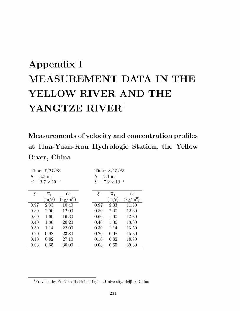
Appendix I
MEASUREMENT DATA IN THE
YELLOW RIVER AND THE
YANGTZE RIVER1
Measurements of velocity and concentration proÞles
at Hua-Yuan-Kou Hydrologic Station, the Yellow
River, China
Time: 7/27/83h = 3.3 mS = 3.7× 10⁻⁴
ξ u1 C(m/s) (kg/m3)
0.97 2.33 10.400.80 2.00 12.000.60 1.60 16.300.40 1.36 20.200.30 1.14 22.000.20 0.98 23.800.10 0.82 27.100.03 0.65 30.00
Time: 8/15/83h = 2.4 mS = 7.2× 10⁻⁴
ξ u1 C(m/s) (kg/m3)
0.97 2.33 11.800.80 2.00 12.300.60 1.60 12.800.40 1.36 13.300.30 1.14 13.500.20 0.98 15.300.10 0.82 18.800.03 0.65 39.30
1Provided by Prof. Yu-jia Hui, Tsinghua University, Beijing, China
234
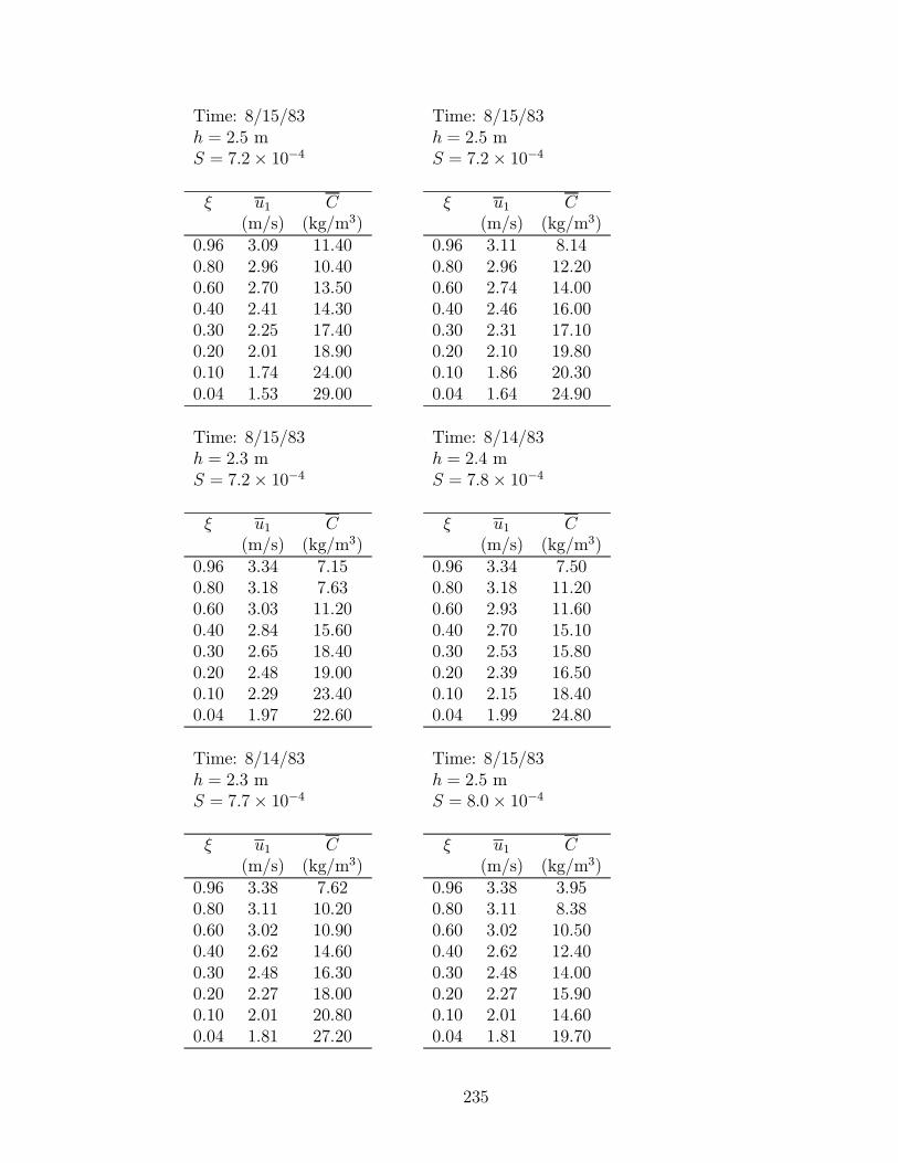
Time: 8/15/83h = 2.5 mS = 7.2× 10⁻⁴
ξ u1 C(m/s) (kg/m3)
0.96 3.09 11.400.80 2.96 10.400.60 2.70 13.500.40 2.41 14.300.30 2.25 17.400.20 2.01 18.900.10 1.74 24.000.04 1.53 29.00
Time: 8/15/83h = 2.5 mS = 7.2× 10⁻⁴
ξ u1 C(m/s) (kg/m3)
0.96 3.11 8.140.80 2.96 12.200.60 2.74 14.000.40 2.46 16.000.30 2.31 17.100.20 2.10 19.800.10 1.86 20.300.04 1.64 24.90
Time: 8/15/83h = 2.3 mS = 7.2× 10⁻⁴
ξ u1 C(m/s) (kg/m3)
0.96 3.34 7.150.80 3.18 7.630.60 3.03 11.200.40 2.84 15.600.30 2.65 18.400.20 2.48 19.000.10 2.29 23.400.04 1.97 22.60
Time: 8/14/83h = 2.4 mS = 7.8× 10⁻⁴
ξ u1 C(m/s) (kg/m3)
0.96 3.34 7.500.80 3.18 11.200.60 2.93 11.600.40 2.70 15.100.30 2.53 15.800.20 2.39 16.500.10 2.15 18.400.04 1.99 24.80
Time: 8/14/83h = 2.3 mS = 7.7× 10⁻⁴
ξ u1 C(m/s) (kg/m3)
0.96 3.38 7.620.80 3.11 10.200.60 3.02 10.900.40 2.62 14.600.30 2.48 16.300.20 2.27 18.000.10 2.01 20.800.04 1.81 27.20
Time: 8/15/83h = 2.5 mS = 8.0× 10⁻⁴
ξ u1 C(m/s) (kg/m3)
0.96 3.38 3.950.80 3.11 8.380.60 3.02 10.500.40 2.62 12.400.30 2.48 14.000.20 2.27 15.900.10 2.01 14.600.04 1.81 19.70
235
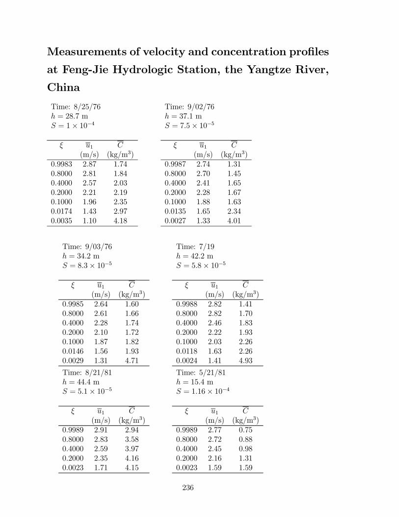
Measurements of velocity and concentration proÞles
at Feng-Jie Hydrologic Station, the Yangtze River,
China
Time: 8/25/76h = 28.7 mS = 1× 10⁻⁴
ξ u1 C(m/s) (kg/m3)
0.9983 2.87 1.740.8000 2.81 1.840.4000 2.57 2.030.2000 2.21 2.190.1000 1.96 2.350.0174 1.43 2.970.0035 1.10 4.18
Time: 9/02/76h = 37.1 mS = 7.5× 10⁻⁵
ξ u1 C(m/s) (kg/m3)
0.9987 2.74 1.310.8000 2.70 1.450.4000 2.41 1.650.2000 2.28 1.670.1000 1.88 1.630.0135 1.65 2.340.0027 1.33 4.01
Time: 9/03/76h = 34.2 mS = 8.3× 10⁻⁵
ξ u1 C(m/s) (kg/m3)
0.9985 2.64 1.600.8000 2.61 1.660.4000 2.28 1.740.2000 2.10 1.720.1000 1.87 1.820.0146 1.56 1.930.0029 1.31 4.71
Time: 7/19h = 42.2 mS = 5.8× 10⁻⁵
ξ u1 C(m/s) (kg/m3)
0.9988 2.82 1.410.8000 2.82 1.700.4000 2.46 1.830.2000 2.22 1.930.1000 2.03 2.260.0118 1.63 2.260.0024 1.41 4.93
Time: 8/21/81h = 44.4 mS = 5.1× 10⁻⁵
ξ u1 C(m/s) (kg/m3)
0.9989 2.91 2.940.8000 2.83 3.580.4000 2.59 3.970.2000 2.35 4.160.0023 1.71 4.15
Time: 5/21/81h = 15.4 mS = 1.16× 10⁻⁴
ξ u1 C(m/s) (kg/m3)
0.9989 2.77 0.750.8000 2.72 0.880.4000 2.45 0.980.2000 2.16 1.310.0023 1.59 1.59
236
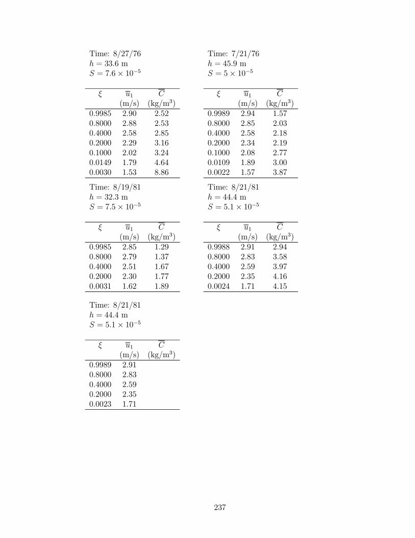
Time: 8/27/76h = 33.6 mS = 7.6× 10⁻⁵
ξ u1 C(m/s) (kg/m3)
0.9985 2.90 2.520.8000 2.88 2.530.4000 2.58 2.850.2000 2.29 3.160.1000 2.02 3.240.0149 1.79 4.640.0030 1.53 8.86
Time: 7/21/76h = 45.9 mS = 5× 10⁻⁵
ξ u1 C(m/s) (kg/m3)
0.9989 2.94 1.570.8000 2.85 2.030.4000 2.58 2.180.2000 2.34 2.190.1000 2.08 2.770.0109 1.89 3.000.0022 1.57 3.87
Time: 8/19/81h = 32.3 mS = 7.5× 10⁻⁵
ξ u1 C(m/s) (kg/m3)
0.9985 2.85 1.290.8000 2.79 1.370.4000 2.51 1.670.2000 2.30 1.770.0031 1.62 1.89
Time: 8/21/81h = 44.4 mS = 5.1× 10⁻⁵
ξ u1 C(m/s) (kg/m3)
0.9988 2.91 2.940.8000 2.83 3.580.4000 2.59 3.970.2000 2.35 4.160.0024 1.71 4.15
Time: 8/21/81h = 44.4 mS = 5.1× 10⁻⁵
ξ u1 C(m/s) (kg/m3)
0.9989 2.910.8000 2.830.4000 2.590.2000 2.350.0023 1.71
237