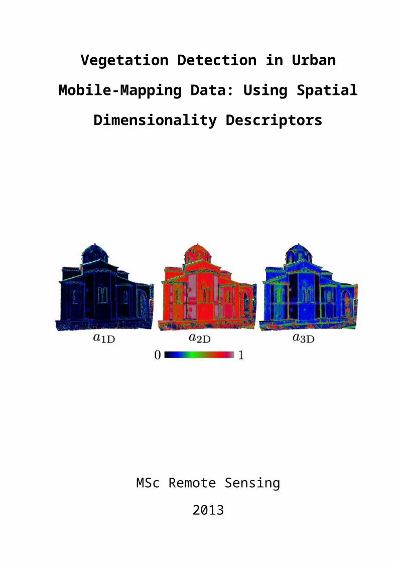
Vegetation Detection in Urban Mobile-Mapping

Data: Using Spatial Dimensionality Descriptors

MSc Remote Sensing

2013

James A Pollock

Supervising Tutor: Dr. Jan Boehm

Table of Contents:

Abstract:...............................................................................................................................................3Acknowledgements:.............................................................................................................................41. Introduction:.....................................................................................................................................5

1.1. Data Acquisition:.......................................................................................................................51.1.1. Light Detection and Ranging:............................................................................................51.1.2. Photogrammetry:................................................................................................................71.1.3. Point Clouds:......................................................................................................................9

1.2. Data Processing/Computer Vision:.........................................................................................101.2.1 Classification:....................................................................................................................10

1.3. Importance of Vegetation:.......................................................................................................111.4. Vegetation Classification:.......................................................................................................15

1.4.1. Spectral Methods:.............................................................................................................151.4.2. Geometric Spatial Methods (Related Work):...................................................................171.4.3 Hybrid Data-fusion Methods:............................................................................................18

1.5. Study Aims & Method Overview:...........................................................................................192. Method:..........................................................................................................................................20

2.1. Data:........................................................................................................................................202.1.2. Full Data Scan-Tile:.........................................................................................................212.1.3. Training Sets:...................................................................................................................212.1.4. Test Sets:..........................................................................................................................21

2.2 Point Cloud Library:.................................................................................................................212.3. Principle Component Analysis:...............................................................................................222.4. Geometric Dimensionality Descriptors:..................................................................................222.5. PCA Neighbourhood Radius Selection:..................................................................................242.6. Classification Rules:................................................................................................................252.7. Writing Classifiers to Point Cloud Data File:.........................................................................27

3. Results and Discussion:..................................................................................................................274. Conclusion:.....................................................................................................................................32Auto-Critique:....................................................................................................................................32References:.........................................................................................................................................33Appendix:...........................................................................................................................................36

A.1. PCA; Descriptor; Classifier:...................................................................................................36A.2. Read xzy/rbgint; Write .PCD file:..........................................................................................40

2

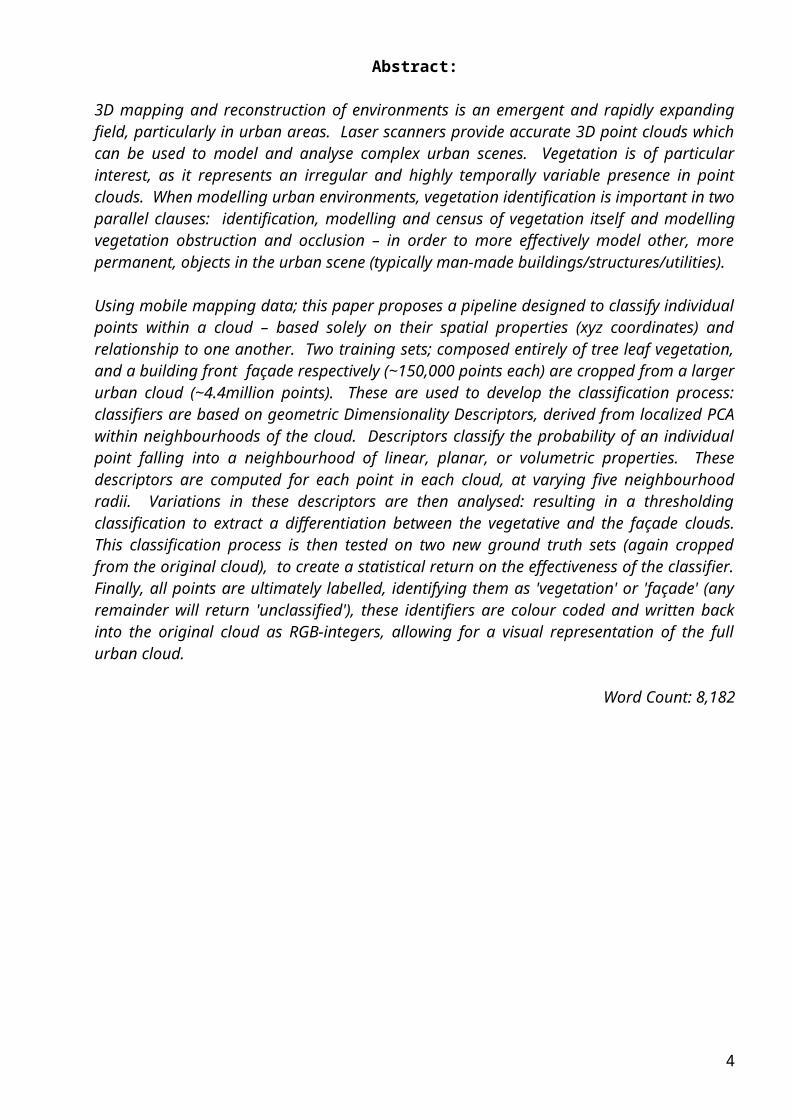
Abstract:

3D mapping and reconstruction of environments is an emergent and rapidly expanding field, particularly in urban areas. Laser scanners provide accurate 3D point clouds which can be used to model and analyse complex urban scenes. Vegetation is of particular interest, as it represents an irregular and highly temporally variable presence in point clouds. When modelling urban environments, vegetation identification is important in two parallel clauses: identification, modelling and census of vegetation itself and modelling vegetation obstruction and occlusion – in order to more effectively model other, more permanent, objects in the urban scene (typically man-made buildings/structures/utilities).

Using mobile mapping data; this paper proposes a pipeline designed to classify individual points within a cloud – based solely on their spatial properties (xyz coordinates) and relationship to one another. Two training sets; composed entirely of tree leaf vegetation, and a building front façade respectively (~150,000 points each) are cropped from a larger urban cloud (~4.4million points). These are used to develop the classification process: classifiers are based on geometric Dimensionality Descriptors, derived from localized PCA within neighbourhoods of the cloud. Descriptors classify the probability of an individual point falling into a neighbourhood of linear, planar, or volumetric properties. These descriptors are computed for each point in each cloud, at varying five neighbourhood radii. Variations in these descriptors are then analysed: resulting in a thresholding classification to extract a differentiation between the vegetative and the façade clouds. This classification process is then tested on two new ground truth sets (again cropped from the original cloud), to create a statistical return on the effectiveness of the classifier. Finally, all points are ultimately labelled, identifying them as 'vegetation' or 'façade' (any remainder will return 'unclassified'), these identifiers are colour coded and written back into the original cloud as RGB-integers, allowing for a visual representation of the full urban cloud.

Word Count: 8,182

3

Acknowledgements:

I would like to make special mention, and thank: my supervisor Dr. Jan Boehm for inspiring me,

and guiding my work on this project; Professor Stuart Robson, for his invaluable advice and

assistance with a particularly tricky piece of code – his patience and willingness to input on a

project outside his supervision was greatly appreciated; Dietmar Backes, for invariably challenging

me to keep trying and consider wider options, when I found myself struggling; and the other

numerous members of the CEGE department whose desks I haunted with my frequent, random,

queries and questions.

4

1. Introduction:

The advent of computer design and graphic modelling technology has created a boom of digital

design products and approaches. An increasing range of professions use 3D graphics technology to

design, plan and evaluate work projects: artists, architects, surveyors, engineers, and many more

professions make use of these techniques on a daily basis. Increasingly the idea has come forward

that digital graphics can not only model fabricated environments, but existing ones. This has a great

number of advantages for users (particularly in the above-mentioned professions) – allowing for

accurate digital representations to be made of real-world scenes (Ikeuchi, 2001). This gives an

existing ground-truth basis for professionals to work from, when planning new projects, renovations

and improvements, and showcasing surveyed data. Building regulators in particular are pushing the

global proliferation of this kind of resource, recording accurate digital representations of new

projects and archiving them alongside blueprints, plans, etc. This gives a comprehensive resource

which can be drawn upon by future workers, referred to as Building Information Modelling (HM

Government UK., 2012). While the promotion of this kind of protocol is highly beneficial, the

issue still faced is that of providing sufficient quantity of, sufficiently accurate, data – for users to

implement these practices. Fortunately in recent years significant advances have been made in

measuring and modelling 3D environments.

1.1. Data Acquisition:

Currently there exist two major methods and supporting technologies for accurately acquiring three

dimensional data from environments. Both methods exist as major industries today, and remain

competitive: each with their own advantages and disadvantages, depending on the context and

application.

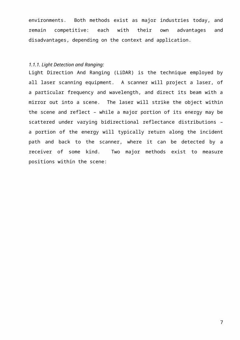
1.1.1. Light Detection and Ranging:

Light Direction And Ranging (LiDAR) is the technique employed by all laser scanning equipment.

A scanner will project a laser, of a particular frequency and wavelength, and direct its beam with a

mirror out into a scene. The laser will strike the object within the scene and reflect – while a major

portion of its energy may be scattered under varying bidirectional reflectance distributions – a

portion of the energy will typically return along the incident path and back to the scanner, where it

can be detected by a receiver of some kind. Two major methods exist to measure positions within

the scene:

5

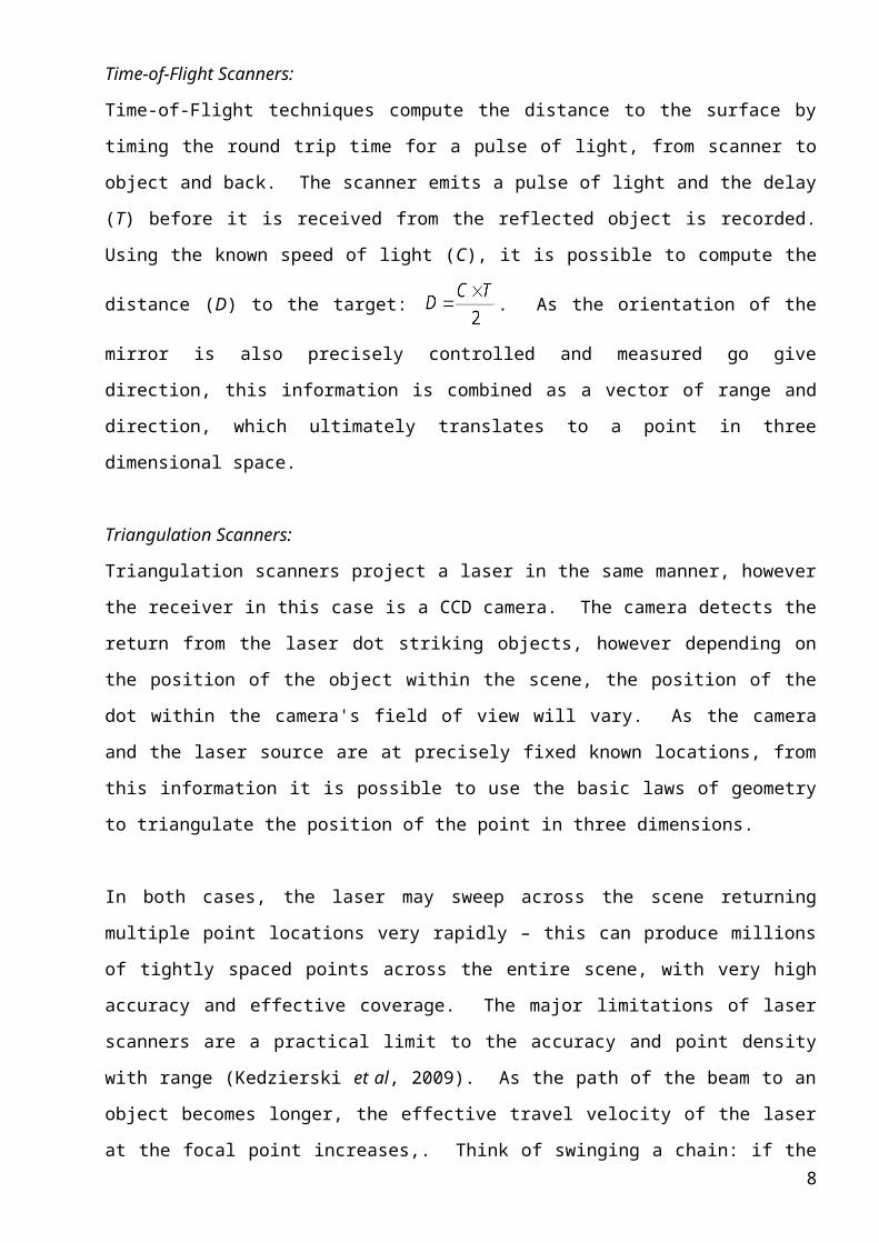
Time-of-Flight Scanners:

Time-of-Flight techniques compute the distance to the surface by timing the round trip time for a

pulse of light, from scanner to object and back. The scanner emits a pulse of light and the delay (T)

before it is received from the reflected object is recorded. Using the known speed of light (C), it is

possible to compute the distance (D) to the target: . As the orientation of the mirror is

also precisely controlled and measured go give direction, this information is combined as a vector

of range and direction, which ultimately translates to a point in three dimensional space.

Triangulation Scanners:

Triangulation scanners project a laser in the same manner, however the receiver in this case is a

CCD camera. The camera detects the return from the laser dot striking objects, however depending

on the position of the object within the scene, the position of the dot within the camera's field of

view will vary. As the camera and the laser source are at precisely fixed known locations, from this

information it is possible to use the basic laws of geometry to triangulate the position of the point in

three dimensions.

In both cases, the laser may sweep across the scene returning multiple point locations very rapidly –

this can produce millions of tightly spaced points across the entire scene, with very high accuracy

and effective coverage. The major limitations of laser scanners are a practical limit to the accuracy

and point density with range (Kedzierski et al, 2009). As the path of the beam to an object becomes

longer, the effective travel velocity of the laser at the focal point increases,. Think of swinging a

chain: if the chain is only a dozen links long the angular velocity at the tip is not greatly

exaggerated compared to the hand swinging it. However if the chain is several dozen links long, the

angular velocity at the tip is greatly increased, in proportion to the swing. As the return can only be

measured at a set interval (while this is done electronically and is extremely fast; it is measuring

returns moving over a distance at the speed of light): the increased angular velocity increases the

distance between returned points – in turn vastly reducing the density of measurements at a range,

and leaving blank areas of undetected space.

6

1.1.2. Photogrammetry:

Photogrammetry has been defined by the American Society for Photogrammetry and Remote

Sensing (ASPRS) as:

"The art, science, and technology of obtaining reliable information about physical objects and the

environment through processes of recording, measuring and interpreting photographic images and

patterns of recorded radiant electromagnetic energy and other phenomena"

In this case it is applied as the practise of using multiple 2D digital images of an object or scene –

taken from a network of mechanically unconnected cameras, to accurately determine the three

dimensional location of points, in a virtual representation of the same space. The principle has been

used for several decades, and was the original method for extracting geometry from remotely

sensed scenes, while the introduction and proliferation of LiDAR and lasers scanning systems has

taken a large market share, it remains a viable technology to this day. With the progression of

modern digital photographic technology, the quality and reliability of images has become great

enough for photogrammetry to once again compete with LiDAR methods, particularly in cases

where the extended fieldwork associated with laser scanning is not appropriate.

Photogrammetric Theory:

The practical process of photogrammetry comprises of a set of mathematical proceedings, as

follows:

Feature extraction: Initially two or more images are compared using the SIFT operator is used to

identify common feature points, this operator is particularly suitable as it is tolerant of both scale

and affine transformation – allowing it to identify corresponding feature points at a variety of

different angles (which is itself necessary for photogrammetry). These identified feature points are

then matched using a RANSAC algorithm, creating clusters of successful matches in each image.

Images can then be orientated to initial values, based on the position of matching features within

separate scenes – this gives further algorithms starting values from which to triangulate position.

Triangulation: Given the image pixel coordinates of each feature (x, y), and the interior orientation

of the camera (xc, yc, c), the collinearity condition can compute the sight lines for each feature,

which can be projected into Object Space. If the camera position and orientation are known, these

sight lines can be intersected from two or more images, giving 3D coordinates in the Object Space

(X, Y, Z).

7

Resection: by using these 3D coordinates given by matched intersecting triangulated sight lines, in a

bundle of four or more (twelve is recommended); the unknowns within the collinearity equations

can be computed via least-squares: giving the exterior orientation of the camera in Object Space

(location: XO, YO, ZO & orientation: O, O, O).

The key trick to photogrammetry is the 'bundle adjustment'. This essentially allows for a group of

images to be computed for the both triangulation and resection, simultaneously – overcoming the

paradoxical problem that to triangulate points you need camera exterior orientation, and that to

orientate the camera you need triangulated 3D coordinates (Geodetic Systems Inc., 2013).

Finally given these accurate camera orientations, the remainder of the pixels within each frame can

be systematically matched in two or more shots, giving 3D point coordinates in Objects Space for

the majority of pixels within the images.

For this to process be effective, the images should typically be taken within a 30º spread, giving

sufficient overlap and sharp angular geometry with respect to the features. Greater than 30º creates

significant angular uncertainty when triangulating the 3D point positions (Kanatani, 1996).

Calibration:

Additionally it should be noted – within the camera the interior orientation is never perfect: even the

best instruments suffer varying distortion in the form of; Principle point position (xp, yp), Radial

lens distortion (k1, k2, k3), decentring lens distortion (p1, p2) and image deformations (a1, a2). These

distortions can be calculated, and corrected for – to avoid systematic errors in the image series

proliferating into the 3D coordinates.

Calibration is computed by including these additional unknown parameters in the bundle

adjustment, described above. The algorithm is able to accommodate these variables and return a

model for the camera distortion, which can then simply be corrected for via an inverse

transformation, producing resampled images. While an attempt at computing these parameters can

be made within any given scene, it is often advisable to calculate them using a calibration rig of

some kind. Using a rig with known geometry and strong reflective targets allows for a very

accurate and reliable calibration adjustment.

8

1.1.3. Point Clouds:

In both the above cases, three dimensional data for environments is recorded on a point by point

basis. Individually these points are relatively useless, however when combined together they can be

seen as a chaotic 3D structure, referred to as a point-cloud: with a minimum of X, Y, Z coordinates

per-point to demonstrate their physical position – and, depending on the method and acquisition

system used, there is potential for spectral data-fusion of; intensity, colour, and photography to be

included (also on a per-point basis). It is reasonable to think of a point-cloud as a series of points

plotted in conventional Cartesian coordinates, a three dimensional graph. While this kind of

method surely existed for thousands of years, since the earliest mathematicians of ancient

civilization, this kind of method has been adapted and used for plotting visual graphics as early as

the 1970s (Welsch, 1976).

Point-clouds are suitable for visually representing complex 3D environments, as (while they are still

composed of large areas of empty space) points congregate where they were reflected by the surface

of objects, creating shadowy representations of these structures. The human eye and mind are adept

at interpreting these representations and 'filling in the blanks' with our deductive ability. This

allows us to look at point-clouds and view them reasonably easily. To further enhance

interpretation users can use software to interpret raw point clouds and manually 'draw' or overlay

more obvious graphical structures (lines, planes, surfaces, and meshes) creating true artificial

graphical representations. However this is a highly acquired skill, and the work is very inefficient

and time consuming. The accuracy of such results also suffers at the whim of human error: having

taken point measurements at a high specification (say English Heritage engineering grade of ~5mm

(Bryan et al, 2009)) a loss of accuracy caused by human interpretation and post-processing of point

locations defeats the purpose, and renders the result flawed.

The demand therefore exists, of an automated and highly accurate system; by which the vast influx

of remotely sensed point-cloud data can be evaluated and post-processed – to provide accurate

results and deliverable materials/statistics for consumers to use in fit-for-purpose applications.

9

1.2. Data Processing/Computer Vision:

Computer vision is the use of computer algorithms to interpret images (both 2D and 3D) in a

manner similar to a human's higher visual processing pathway. There are two principle foci:

perception and understanding – perception refers to the ability to register features within an image,

while understanding is the ability to determine what these features specifically represent (Sonka et

al, 2008). Digital data sets can be considered as grids of numerical values: for example a typical

digital photograph is a two dimensional array of intensity values (typically with a Red, Green, and

Blue value) for each individual pixel. Likewise a point-cloud is a three dimensional irregular array,

where each 'pixel' is a point with an X, Y, and Z value in space. Computer vision methods use

mathematical algorithms to extract information about individual (or groups of) pixels, with respect

to their neighbours. In their most simple form this allows for the detection of edges within the

scene, by simply analysing or amplifying the gradient of the difference in value between

neighbouring pixels. The Canny operator (Canny, 1986) is a standard example, which is still used

in computer vision across the world today – due to its simplicity and effectiveness.

As computers became more powerful, and the field of computer vision developed it became

possible to extract more than just simple edge detection from digital data sets. As perception

typically represents the more straight forward challenge, and extracting features from images

became more streamlined – much emphasis has shifted to the more complex challenge of equipping

computers with methods to understand specifically what features have been detected.

1.2.1 Classification:

While measuring and modelling absolute 3D location/shape of objects is clearly important, there

exists a parallel field of allocating classification to individual (or groups of) points – in order to

identify them as belonging to a particular class. Instruments can use data on spatial position and/or

reflectance to evaluate factors such as; surface roughness, colour, temperature, density and

thickness. From these responses classes can be constructed to identify points which adhere to any

combination of rules (Exelis Visual Information Studios, 2013). These classes can be arbitrary for

very specific user purposes, but more typically they include information such as the material of the

object, or the type of object it is: e.g. bare earth, vegetation, water.

Many of these classification systems were developed in satellite-based remote sensing operations,

working on a large resolution (>500m2) spectral data to evaluate land-surface properties. Generally

working on the simplest level, these methods identify individual pixels as belonging to a pre-

defined class – based upon their spectral reflectance values. A number of workflows of this nature

are still in use today, providing highly effective data for analysts and researchers.

10

For example: the NASA run MODIS Snow Product (NASA, 2012) uses a 36-chanel visible to

thermal-infrared spectrometer to gather data in 500m2 resolution. Each pixel is then evaluated

against a series of classification rules; thresholding against reflectance properties across the multiple

channels, in order to establish its content. Similarly Burned Earth products where burned ground

area is detected by evaluating pixels for low spectral reflectivity mainly at visible wavelengths (e.g.

darkened ground/ash from recent burn events). Alternatively, the BIRD satellite based fire-

detection product looks for fires in real time, by differencing pixels for spectral reflectance from the

3.7m and 11m wavelengths and inverting Planck's function to establish the emitted energy of a

pixel (and therefore the ferocity of the burn event) (Wooster et al, 2003).

In recent times these types of systems have also been transferred to applications in the more

localized, mobile mapping community. Identification of differing objects in an urban scene is

highly important for a range of users.

1.3. Importance of Vegetation:

The focus in this instance will be vegetation identification in urban environments. Vegetation

identification is important for two major reasons:

The prospecting, census and classification of vegetation itself is highly important in a range of

applications, both commercial and environmental:

A large aspect of this is the environmental factors of vegetation presence and change, which are

heavily pushed in the public eye – both in media and politics. Growth of vegetation (both aquatic

and terrestrial, though in this case our focus is on the latter) actively absorbs carbon from the

atmosphere, converting it into carbohydrates found in plant starches and sugars – a process termed

as biosequestration (Garnaut, 2008). This process acts as a vast global carbon sink, effectively

maintaining the balance of CO2 in the atmosphere. Recent studies conclusively implicate human

activities, such as industrial scale burning of fossil fuels and wide spread deforestation, as actively

increasing global atmospheric CO2 levels – potentially with subsequent driving effects on global

climate change (Houghton et al, 2001). The Intergovernmental Panel on Climate Change (IPCC)

has been specifically set up to address this issue; mainly through regulation of any particular

activities, which a may nation undertake (both positive and negative), that effect global climate.

With the establishment of acts such as the Kyoto Protocol (UNFCCC, 2013a): 'Land Use, Land-Use

Change and Forestry' (LULUCF) actions are increasingly being used as highly cost-effective, and

active environmentally protecting measures, to offset carbon emissions and meet protocol climate-

11

change budgets (UNFCCC, 2013b). These actions are mainly focused on avoiding/reducing

deforestation and reforestation.

Identifying the occurrence of vegetation also has many commercial applications:

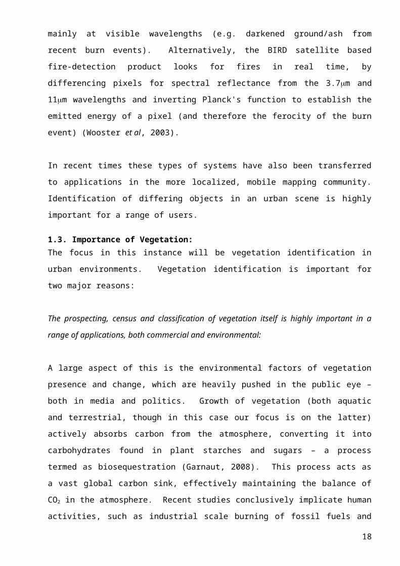
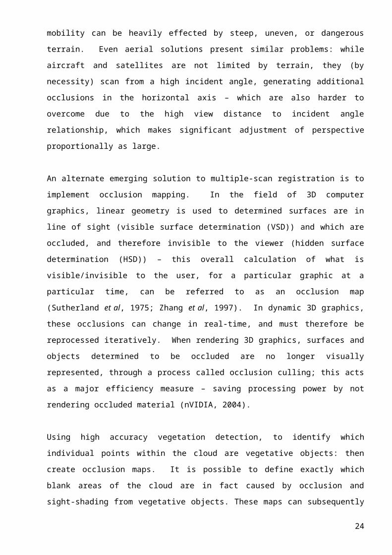
Agriculture stands as the largest and most profitable form of land-use on the planet, not to mention

a necessary activity to support human populations. The Food and Agricultural Organization of the

United Nations' (FAO) FAOSTAT project estimates the global value of agricultural production at

$881billion [Figure 1.3.a], in the year of 2011 (note this figure is based on the top twenty

agricultural products worldwide, and does not include the yield from livestock-producing pasture –

which significantly increases the value ~$1.4trillion).

Figure 1.3.a:

Source: Food and Agricultural Organization of the United Nations (2013).

12

Forestry represents another vast and valuable global industry. The majority of existing temperate

forests (mostly within the northern hemisphere: boreal region) are under some form of commercial

management representing huge value as timber alone. In addition they generate income from: non-

timber-forest-products (NTFPs); areas of scientific interest/research; biodiversity; tourism and

recreation; and carbon-budget sinks. Likewise tropical forests represent a huge source of income,

and while a smaller percentage of them are managed, Pearce (2001) suggests that the average

economic value of forests lies between 1,195-15,990 $/ha/pa for tropical forests, worldwide.

The ability to accurately monitor stocks and fluxes of vegetation is highly relevant to these

government policies and their related industries, it allows for more reliable inventories, and

subsequently higher quality models of supply/demand, forecasts, and predictions: overall creating a

more efficient business/policy practice.

On a more localised scale, the accurate identification and record of individual occurrences of

vegetation (namely trees and large plants) can be essential to engineers and planners; when dealing

with vegetation that infringes or interferes with other elements of current (or proposed) human

infrastructure. For example, over time the boughs of large trees may collide with

buildings/structures, and their roots can inhibit or damage subterranean infrastructure (sewers,

utilities and even building foundations).

In more specific circumstances, the accurate measurement of the presence and physical properties

of vegetation, may be auxiliary to the accurate measurement of an alternate target object or type:

In the instance of environment modelling, vegetation can represent an obstructive object-type,

within the scene. When planners, architects, and other surveyors require to model the man-made

infrastructure of an (urban) environment – the presence of vegetation can hinder the otherwise

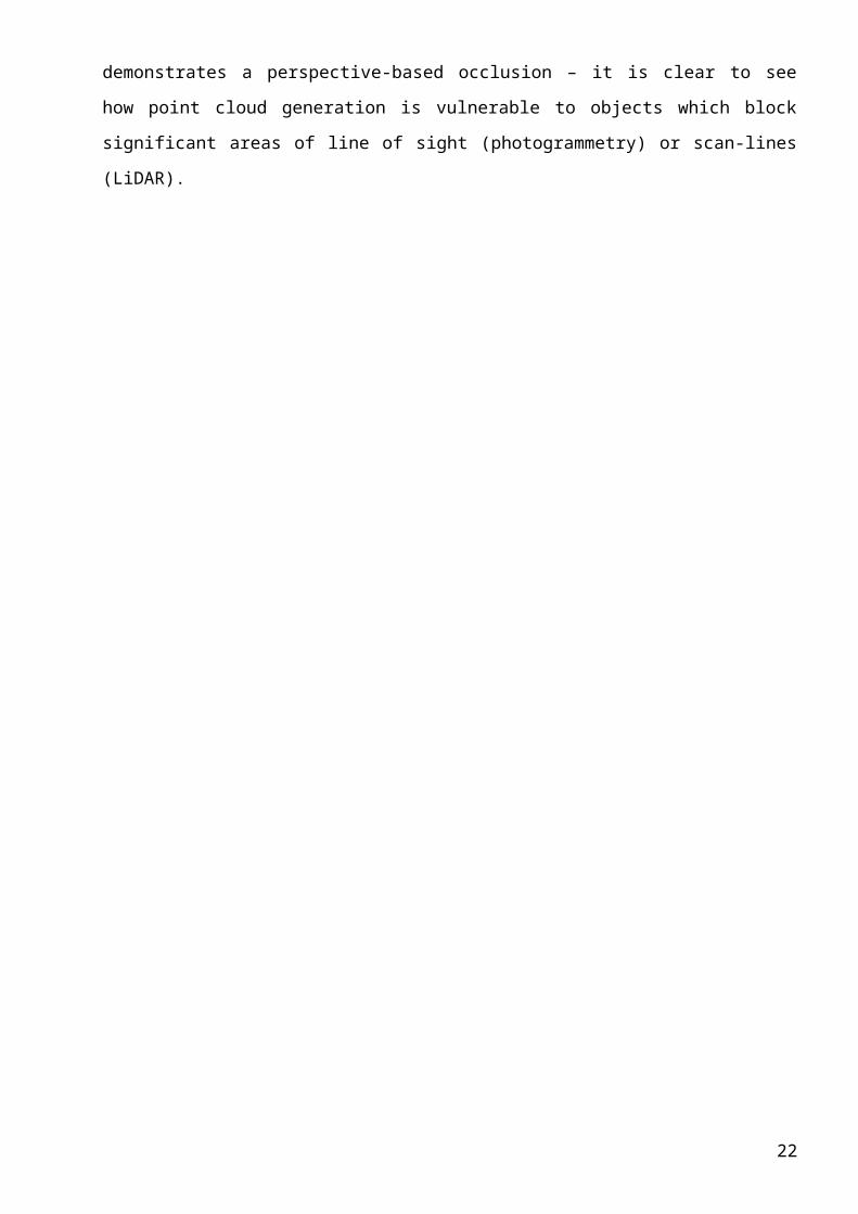
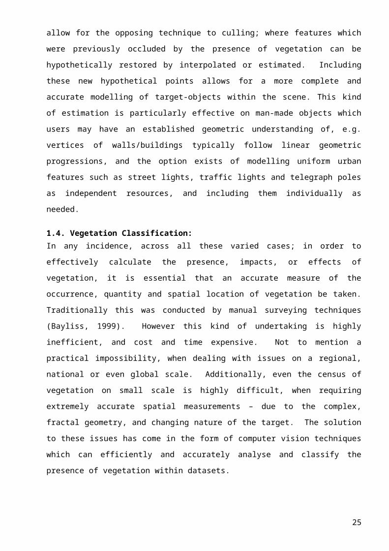
accurate measurement by specialist instruments (Monnier et al, 2012). Figure 1.3.b. demonstrates a

perspective-based occlusion – it is clear to see how point cloud generation is vulnerable to objects

which block significant areas of line of sight (photogrammetry) or scan-lines (LiDAR).

13

Figure 1.3.b:

Note: the blank area where the parked vehicle blocks scan lines.

While both methods for creating point-cloud data sets are susceptible to this kind of vegetation

occlusion, It should be noted that this problem can be significantly overcome with the use of cross-

scan registration: combining multiple point-clouds with separate origins (and therefore scan

perspective) to resolve perspective based occlusion issues. The drawback of this method is that

taking multiple scans is not always possible; and even when achievable, increases the time, cost,

and complexity of surveying projects. In particular for mobile mapping projects, where survey

routes can be between tens and thousands of kilometers, it is extremely inefficient for the scan

system to have to cover its tracks multiple times, in the (unguaranteed) hope of achieving a different

scan perspective – even repeat passes may not achieve a more desirable scan angle, as mobile

platforms are still limited by the path they can physically follow. In the case of urban environments

equipment is typically mounted on a vehicle and thusly is predominantly effected by the law of the

roads, in less developed rural/remote areas equipment mobility can be heavily effected by steep,

uneven, or dangerous terrain. Even aerial solutions present similar problems: while aircraft and

satellites are not limited by terrain, they (by necessity) scan from a high incident angle, generating

additional occlusions in the horizontal axis – which are also harder to overcome due to the high

view distance to incident angle relationship, which makes significant adjustment of perspective

proportionally as large.

An alternate emerging solution to multiple-scan registration is to implement occlusion mapping. In

the field of 3D computer graphics, linear geometry is used to determined surfaces are in line of sight

(visible surface determination (VSD)) and which are occluded, and therefore invisible to the viewer

(hidden surface determination (HSD)) – this overall calculation of what is visible/invisible to the 14

user, for a particular graphic at a particular time, can be referred to as an occlusion map (Sutherland

et al, 1975; Zhang et al, 1997). In dynamic 3D graphics, these occlusions can change in real-time,

and must therefore be reprocessed iteratively. When rendering 3D graphics, surfaces and objects

determined to be occluded are no longer visually represented, through a process called occlusion

culling; this acts as a major efficiency measure – saving processing power by not rendering

occluded material (nVIDIA, 2004).

Using high accuracy vegetation detection, to identify which individual points within the cloud are

vegetative objects: then create occlusion maps. It is possible to define exactly which blank areas of

the cloud are in fact caused by occlusion and sight-shading from vegetative objects. These maps can

subsequently allow for the opposing technique to culling; where features which were previously

occluded by the presence of vegetation can be hypothetically restored by interpolated or estimated.

Including these new hypothetical points allows for a more complete and accurate modelling of

target-objects within the scene. This kind of estimation is particularly effective on man-made

objects which users may have an established geometric understanding of, e.g. vertices of

walls/buildings typically follow linear geometric progressions, and the option exists of modelling

uniform urban features such as street lights, traffic lights and telegraph poles as independent

resources, and including them individually as needed.

1.4. Vegetation Classification:

In any incidence, across all these varied cases; in order to effectively calculate the presence,

impacts, or effects of vegetation, it is essential that an accurate measure of the occurrence, quantity

and spatial location of vegetation be taken. Traditionally this was conducted by manual surveying

techniques (Bayliss, 1999). However this kind of undertaking is highly inefficient, and cost and

time expensive. Not to mention a practical impossibility, when dealing with issues on a regional,

national or even global scale. Additionally, even the census of vegetation on small scale is highly

difficult, when requiring extremely accurate spatial measurements – due to the complex, fractal

geometry, and changing nature of the target. The solution to these issues has come in the form of

computer vision techniques which can efficiently and accurately analyse and classify the presence

of vegetation within datasets.

1.4.1. Spectral Methods:

Spectral methods for identifying vegetation have been effectively used for some time: in the form of

Vegetation Indices (VI). As in the above satellite classification examples, these function by

thresholding or differencing reflectance at specific radiometric wavelengths (NASA, 2013). The

purpose of vegetative leaf surface is to conduct photosynthesis for the plant-organism possessing it:

this process involves the absorption of photons from incoming electromagnetic waves (light). Thus,

15

by its very nature, vegetative surfaces strongly absorb particular elements of the spectrum and

reflect others. The reason vegetation predominately appears as green leaves is due to the

photosynthetic compounds chlorophyll not absorbing light energy in this region. This kind of

absorption and reflectance goes on to happen outside the visible spectrum, experiencing a

significant change in the near infrared band (NIR) – where plant cell structures strongly reflect NIR

light.

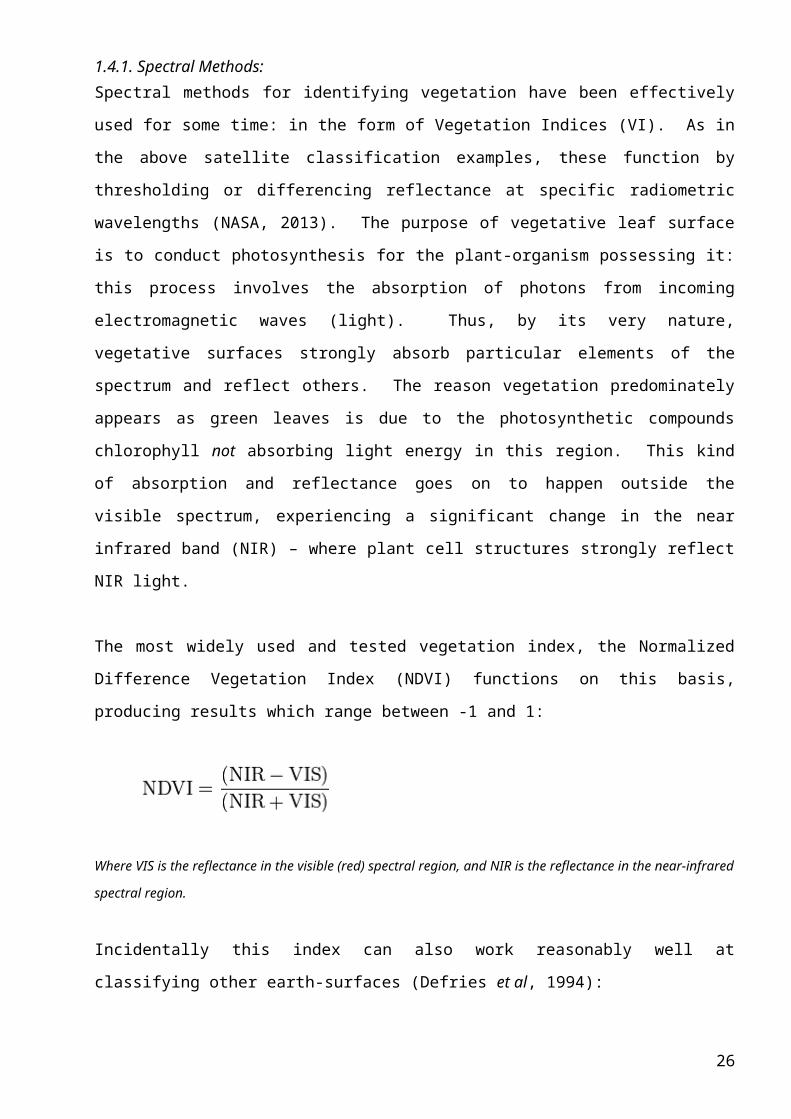
The most widely used and tested vegetation index, the Normalized Difference Vegetation Index

(NDVI) functions on this basis, producing results which range between -1 and 1:

Where VIS is the reflectance in the visible (red) spectral region, and NIR is the reflectance in the near-infrared spectral

region.

Incidentally this index can also work reasonably well at classifying other earth-surfaces (Defries et

al, 1994):

− Vegetation canopies generally exhibit positive values (~0.3-0.8).

− Soils show low positive values (~01.-0.2)

− Snow, ice and clouds (highly spectrally reflective surfaces) exhibit negative values (~-0.5)

− Water (ocean, seas, lakes) exhibits high absorption in all bands resulting in a very low value

(~0.0)

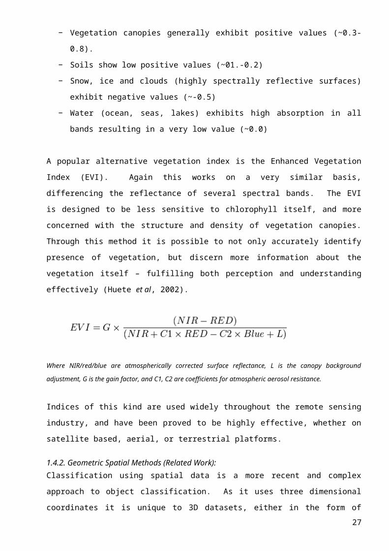
A popular alternative vegetation index is the Enhanced Vegetation Index (EVI). Again this works

on a very similar basis, differencing the reflectance of several spectral bands. The EVI is designed

to be less sensitive to chlorophyll itself, and more concerned with the structure and density of

vegetation canopies. Through this method it is possible to not only accurately identify presence of

vegetation, but discern more information about the vegetation itself – fulfilling both perception and

understanding effectively (Huete et al, 2002).

Where NIR/red/blue are atmospherically corrected surface reflectance, L is the canopy background adjustment, G is

the gain factor, and C1, C2 are coefficients for atmospheric aerosol resistance.

16

Indices of this kind are used widely throughout the remote sensing industry, and have been proved

to be highly effective, whether on satellite based, aerial, or terrestrial platforms.

1.4.2. Geometric Spatial Methods (Related Work):

Classification using spatial data is a more recent and complex approach to object classification. As

it uses three dimensional coordinates it is unique to 3D datasets, either in the form of point-clouds,

or digital elevation models (DEMs). The former being irregular points with XYZ coordinates, the

latter being an adjusted raster data-format where pixels locations establish X and Y locations, while

pixel values establish a Z-axis.

Spatial classifiers come in a number of forms, however a trend in workflows appears to be the

concept of using data to 'train' a specific algorithm (Duda et al 2012): e.g. ground truth data is

selected specifically to represent the desired class to be identified. This data is then evaluated and

algorithms generated to recognize the spatial patterns present between points. Having used this

training set, algorithms can then be tested and tuned on other examples to establish their

effectiveness (if necessary returning to the original training step many times before proceeding).

An approach of this nature is entirely logical, as it strongly reflects the manner in which humans

(and animals) learn and make deductions.

The paper by Toldo et al (2009) on 3D object classification is a strong example of this kind of

workflow. In their case objects were segmented and their spatial properties were reduced into a

histogram of "3D visual word occurrences": essentially classifying a known object by categorizing

sub-object segments – then defining that object type as containing a specific

number/combination/distribution of these segments. New objects can then be tested and classified

by the same segmentation and numerical evaluation of their spatial parts. A similar example is

conducted by Golovinskiy et al (2009), using shape feature vectors, as oppose to the histogram

approach.

Other researchers have used more geometric approaches, using reductive algorithms (such as Least-

squares, or the more robust RANSAC approach) in an attempt to fit regular geometric shapes into

clouds. Fitting for planes, cylinders, pipes and other established shapes can help in identify target

objects (or counter-identifying: e.g. cleaning established non-target objects from the cloud). This

sort of approach is particularly effective where the environment is known to contain objects of a

regular geometric type: e.g. indoor environments with surfaces, planes and right angled vertices;

manufacturing/industrial environments with pipes, cylinders or supports of known dimension

(Rutzinger et al, 2009; Newman et al, 1993).

17

More recent attempts combine object classification with more complex shape description

frameworks: such as the study by Velizhev et al (2012) where scenes are segmented, and objects

recognized on the basis of an implicit shape model (IMS). Other complex object recognition

methods include the use of: spin images (Johnson, 1999); extended Gaussian images (Horn, 1984);

angular spin images (Endres et al, 2009); FPFH (Rusua et al, 2009); and 3D SURF (Knopp et al,

2010).

In the case of specific vegetation detection, a number of attempted works exist: the follow up study

by Rutzinger et al (2010); Antonarakis et al (2008) attempt vegetation classification through texture

analysis of aerial LiDAR data; Monnier et al (2012) propose a vegetation detector based on 3D

dimensionality descriptors and 2D clustering algorithms. While promising, these methods are still

subject to testing and development, with many further studies to follow – improving and expanding

upon the principles laid down in the last decade.

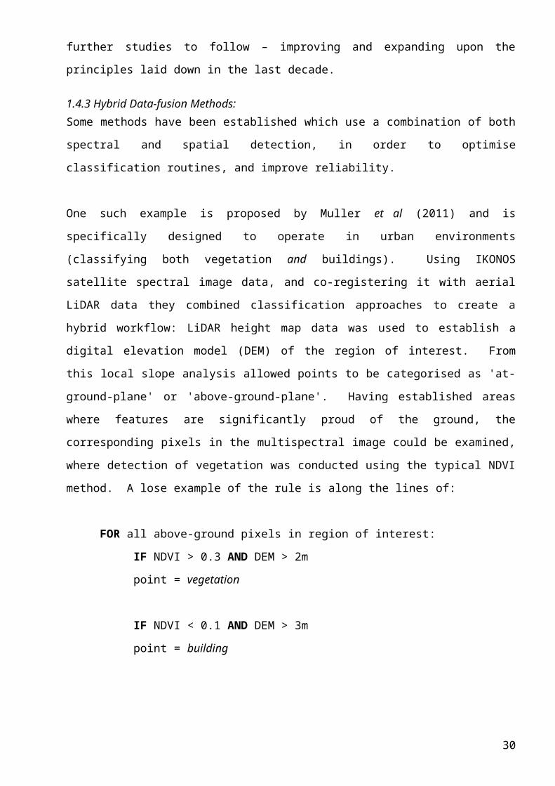
1.4.3 Hybrid Data-fusion Methods:

Some methods have been established which use a combination of both spectral and spatial

detection, in order to optimise classification routines, and improve reliability.

One such example is proposed by Muller et al (2011) and is specifically designed to operate in

urban environments (classifying both vegetation and buildings). Using IKONOS satellite spectral

image data, and co-registering it with aerial LiDAR data they combined classification approaches to

create a hybrid workflow: LiDAR height map data was used to establish a digital elevation model

(DEM) of the region of interest. From this local slope analysis allowed points to be categorised as

'at-ground-plane' or 'above-ground-plane'. Having established areas where features are significantly

proud of the ground, the corresponding pixels in the multispectral image could be examined, where

detection of vegetation was conducted using the typical NDVI method. A lose example of the rule

is along the lines of:

FOR all above-ground pixels in region of interest:

IF NDVI > 0.3 AND DEM > 2m

point = vegetation

IF NDVI < 0.1 AND DEM > 3m

point = building

18

This kind of data fusion technique has been proved to be highly effective, and is an expanding

approach to classification in many fields – as it can be used to effectively overcome the individual

limitations of techniques, by combining their strengths (Duda et al, 1999; Song et al, 2002; Muller

et al, 2011).

1.5. Study Aims & Method Overview:

While inclusion of spectral methods has been proved to be very effective; as pointed in section

1.4.1., the only common property of all raw point-cloud data is simply the spatial XYZ coordinates.

For this reason the following work will attempt to establish a classification system based solely on

XYZ spatial data, which can be used universally across point-clouds regardless of any data fusion

for intensity, reflectance, colour, or other radiometric data.

Our aim is to produce a generic workflow which can be used to identify occurrence of vegetation in

dense urban scenes. As the majority of urban environments contain planar, façade surfaces; this

methodology is designed to create and apply two specific classifiers to point clouds; identifying

points individually as belonging to either generic façade objects, or vegetation objects, within the

urban scene. Any remaining points not adhering to these classifier rules will for the time being be

regarded as an 'unclassified', and identified thusly.

This methodology is partially based on work conducted on dimensionality descriptors by Demantké

et al (2011) – classifying points based on the occurrence of Linear (D1), Planar (D2) or Volumetric

(D3) shape properties, within their neighbourhood. The theory is that flat façade objects exhibit

strong planar nature, while the chaotic, fractal nature of vegetation exhibits strong volumetric

nature. Having conducted principle component analysis (section 2.3.), and subsequently computing

dimensionality descriptors for each individual point within a cloud (section 2.4): the initial

assumption might be that façade can simply be classified for all points where the planar descriptor

(D2) is the maximum, similarly vegetation can be classified for all points where the volumetric

descriptor (D3) is the maximum. In reality these descriptor allocations vary significantly, depending

on both the overall point cloud and local neighbourhood point-densities. Therefore descriptors

were computed at a range of five increasing neighbourhood radii; and the results then plotted and

analysed (section 2.4.), to compose a classification system based on a pairing of descriptor

thresholding rules (section 2.5). Finally this classification was tested, applying the identifiers to

new tests sets – and both statistically and visually representing the outcome (section 3.)

19

2. Method:

2.1. Data:

Due to the speed, efficiency and reliability of Laser scanners in mobile mapping – the workflow

was composed and tested using LiDAR data. This does not necessarily limit it's generic application

on point-cloud data from other sources. However, some numerical specifics of the

processing/classification may require tuning, on a case-by-case basis.

2.1.1. Collection:

Data was collected prior to this study, and the proceedings here were not personally responsible for

the raw data acquisition.

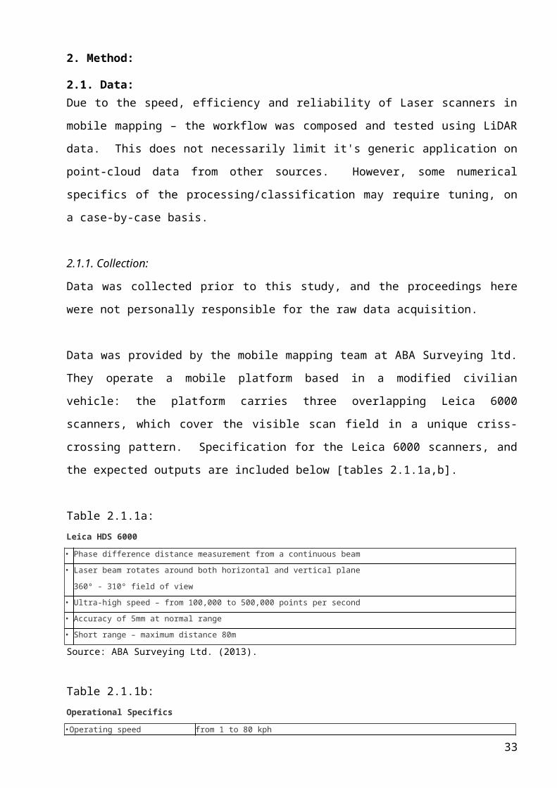
Data was provided by the mobile mapping team at ABA Surveying ltd. They operate a mobile

platform based in a modified civilian vehicle: the platform carries three overlapping Leica 6000

scanners, which cover the visible scan field in a unique criss-crossing pattern. Specification for the

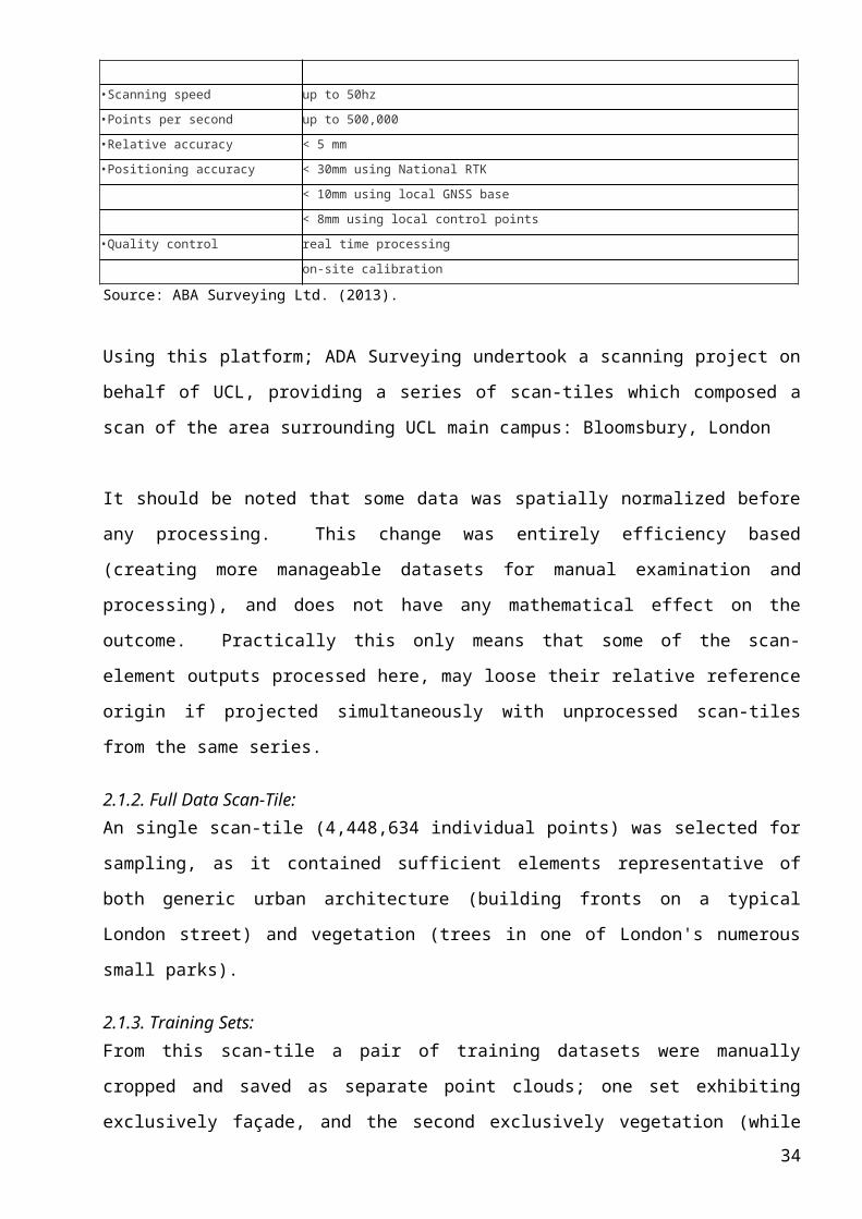
Leica 6000 scanners, and the expected outputs are included below [tables 2.1.1a,b].

Table 2.1.1a:

Leica HDS 6000

• Phase difference distance measurement from a continuous beam

• Laser beam rotates around both horizontal and vertical plane

360º - 310º field of view

• Ultra-high speed – from 100,000 to 500,000 points per second

• Accuracy of 5mm at normal range

• Short range – maximum distance 80m

Source: ABA Surveying Ltd. (2013).

Table 2.1.1b:

Operational Specifics

•Operating speed from 1 to 80 kph

•Scanning speed up to 50hz

•Points per second up to 500,000

•Relative accuracy < 5 mm

•Positioning accuracy < 30mm using National RTK

  < 10mm using local GNSS base

  < 8mm using local control points

•Quality control real time processing

  on-site calibration

Source: ABA Surveying Ltd. (2013).

20

Using this platform; ADA Surveying undertook a scanning project on behalf of UCL, providing a

series of scan-tiles which composed a scan of the area surrounding UCL main campus:

Bloomsbury, London

It should be noted that some data was spatially normalized before any processing. This change was

entirely efficiency based (creating more manageable datasets for manual examination and

processing), and does not have any mathematical effect on the outcome. Practically this only means

that some of the scan-element outputs processed here, may loose their relative reference origin if

projected simultaneously with unprocessed scan-tiles from the same series.

2.1.2. Full Data Scan-Tile:

An single scan-tile (4,448,634 individual points) was selected for sampling, as it contained

sufficient elements representative of both generic urban architecture (building fronts on a typical

London street) and vegetation (trees in one of London's numerous small parks).

2.1.3. Training Sets:

From this scan-tile a pair of training datasets were manually cropped and saved as separate point

clouds; one set exhibiting exclusively façade, and the second exclusively vegetation (while

approximately the same size spatially they were ~100,000 and ~200,000 points respectively).

These sets were analysed and used to develop the vegetation identification workflow below.

2.1.4. Test Sets:

Finally, a second pair of test sets were cropped from the same original scan-tile: again of

approximately the same spatial size, and representing façade and vegetation respectively. While

illustrative the same generic features, they were specifically cropped from separate areas to the

original training sets: as these sets are required to be unbiased, when used to evaluate the

effectiveness of the developed workflow.

2.2 Point Cloud Library:

Point Cloud Library (PCL) is a stand alone, open source, binary package written and compiled in

C++. Designed and written by a global collaboration of developers across the remote sensing and

geomatics communities: the library contains a vast range of functions designed specifically to

handle point-cloud data, including multiple techniques for: data refinement/noise reduction;

filtering; segmentation; surface reconstruction; and modelling.

This project takes advantage of a number of these standard prebuilt techniques, and includes them

into the workflow. As PCL is written in C++ and designed to work with the Microsoft Visual

Studio 2010 compiler, the majority of the workflow here follows this convention, and used these

packages.21

2.3. Principle Component Analysis:

Principle Component Analysis (PCA) evaluates the spatial distribution of points within a given

LiDAR cloud (or in this case neighbourhood): Let x i = (xi yi zi)T and = i = 1,n xi the centre of

gravity of the n LiDAR points of . Given , the 3D structure tensor is

defined by . Since C is a symmetric positive definite matrix, an eigenvalue

decomposition exists and can be expressed as , where R is a rotation matrix, and a

diagonal, positive definite matrix, known as eigenvector and eigenvalue matrices, respectively. The

eigenvalues are positive and ordered so that . , , denotes the

standard deviation along the corresponding eigenvector . Thus, the PCA allows to retrieve the

three principle directions of , and the eigenvalues provide their magnitude. The average

distance, all around the centre of gravity, can also be modelled by a surface. The shape of is

then represented by an orientated ellipsoid. The orientation and size are given in R and : R turns

the canonical basis in to the orthonormal basis and transforms the unit sphere to an

ellipsoid (σ1, σ2 and σ3 being the lengths of the semi-axes). From this neighbourhood ellipsoid

shape, it is now possible to consider the point distribution in terms of volumetric geometry, or

dimensionality (Demantké et al, 2011).

2.4. Geometric Dimensionality Descriptors:

The eigenvalues extracted from PCA numerically describe the 3D distribution of points in the cloud

– while possessing arbitrary orientation (eigenvectors) and magnitude (highly dependant on the

scale of the cloud, and the size of the neighbourhood in question). Having used PCA to

approximate the spatial distribution of points in the neighbourhood: as ellipsoid with axis Vi, and

axis lengths there are three extreme cases:

: one main direction: linear neighbourhood

: two main directions: planar neighbourhood

: isotropy: volumetric neighbourhood

Dimensionality descriptors are used to normalize these eigenvalue relationships, and define how

close the individual neighbourhood shape is to one of these three, extreme configurations:

Linear descriptor:

Planar descriptor:

Volumetric descriptor:

22

When computed thusly, the value of each dimensionality descriptor falls between 0 and 1 –

representing the probability that a single point (at a defined neighbourhood) adheres to that

descriptor. Where variations in point cloud density and small selection radius created

neighbourhoods of critically too few points: PCA failed to produce eigenvalues. These cases were

defaulted to , , : thusly creating failed descriptors with their values set to 0.

While the descriptors are somewhat representative of classification at this point, Figure 2.4.a

demonstrates their variability and vagueness in a LiDAR scene, when selected at a single

neighbourhood size. The linear descriptor functions reasonably effectively classifying edges, but

only with a low probability ~25-50%. The planar descriptor dominates the majority of the scene,

detecting the building faces with a very high probability ~90-100%, while exhibiting some

detection ~30% on linear edge features. The volumetric descriptor functions poorly, only

highlighting small areas with any great probability. Due to the overlap, and similar probabilities,

between the linear and planar descriptors, it actually remains difficult to classify objects just from

this data (e.g. an edge object exhibits ~30% intensity in linear, planar, and volumetric descriptors).

It is for this reason that five increasing radii were selected and descriptors computed for each

neighbourhood.

Figure 2.4.a

Demonstration of values for each dimensionality descriptor on a single scene – source: Demantké et al (2012).

Note: the code for the above processing of PCA and computing/writing Dimensionality Descriptors

is included in Appendix: A.1.

2.5. PCA Neighbourhood Radius Selection:

To evaluate descriptor values for any shape or pattern that could be used to differentiate vegetation

and façade objects, the above PCA and descriptors computation was repeated for both training

23

clouds, at a range of five PCA neighbourhood radii. Demantké et al (2011) propose that the

minimum and maximum radii in this range would be likely to vary between different point clouds,

depending on; data collection method, and morphology of features in the area of interest. The lower

bound is typically driven by the point cloud noise, sensor specifications, and any computational

restraints. The upper bound is context sensitive, and is generally suitable at a similar size to the

largest objects in the scene – typically 2-5m in urban mobile mapping scenes, and in the tens of

meters for aerial data.

On this basis neighbourhood radii were proposed in a range, at: 0.1m, 0.25m, 0.5m, 1m, and 2.5m.

This lower limit is close to the point at which the relative point accuracy of the cloud (0.05m)

makes any higher precision on the part of PCA redundant. The higher accuracy corresponds to the

convention for terrestrial mobile mapping.

24

2.6. Classification Rules:

A random sample of 1000 point descriptors from each training set were chosen for visualization,

and evaluation (Figure 2.5.a).

Figure 2.5.a:

X-axis: neighbourhood radii; Y-axis: descriptor intensity

Note: random descriptor sampling and plotting were conducted in Mathworks: Matlab package,

and are not part of the included classifier script.

The graphical representation further confirms that the descriptors alone are not sufficient to classify

point-object type, with great variation, and significant overlap between the distinct façade and

vegetation plots. In particular the linear descriptor (D1) is highly variable, offering no major

discernable differentiation between the façade and vegetation tests. It is also clear that the linear

25

descriptor is highly prevalent at low neighbourhood radii (< 0.5m), making these small

neighbourhoods poor for any classification scheme.

Visual analysis of the six plots suggests that:

− i & ii: D1 is far too chaotic, not exhibiting any significant discernable difference between

vegetation and façade objects across the range of radii. This descriptor was essentially

discarded at this point, however this is specific to this work – and the descriptor may still

have merit in other studies, particularly if attempting to classify different object types.

− iii: D2 shows a trend of points rating above 0.2 for façade objects across the majority of the

radii.

− iv: A converse trend exists, of virtually no points rating above 0.6 for vegetation across the

majority of radii.

− v: D3 shows a strong trend of low values for façade objects, with the vast majority of points

exhibiting a rating below 0.3 at all radii.

− vi: Finally there is little specific information that can be discerned from the D3 descriptor

solely for vegetation objects.

Following this qualitative evaluation of the descriptor plots, it was ultimately concluded that the

most obvious set of rules for classification are as follows:

FOR points in cloud:

IF ((D2 <= 0.6) AND (D3 >= 0.2)) @ PCA radius = 1.5

point = vegetation

ELSE

IF ((D2 >= 0.2) AND (D3 <= 0.2)) @ PCA radius = 1.5

point = façade

ELSE

point = unclassified

In this case the greatest differentiation between vegetation and façade descriptors appears at ~1.5m

PCA neighbourhood radii. This is likely a product of the data type and content of the scene, and

probably unique to this data set. However, it conveniently allows for a vast increase in processing

efficiency, as the radii repetition loop could be removed from the PCA/Dimensionality script, and a

set radius of 1.5m be used to generate all descriptors required for classification.

26

2.7. Writing Classifiers to Point Cloud Data File:

Point Cloud Data (.pcd) files are the conventional format for point-clouds when using PLC. They

are also transferable across a range of industry standard packages, including; Leica Cyclone,

Autodesk Recap (and other Autodesk products, as per the Autodesk design philosophy), and

ccViewer/CloudCompare.

In order to visualize the point-clouds with their new classifiers, the original .xyz files were read in

parallel to the new classifier vector .txt files, iterating through each line and combining them to

write into a <pcl::PointXYZRGB> type .pcd file.

Note: the code for this processing, to read + write clouds/classifiers to .pcd is included in

Appendix: A.2.

3. Results and Discussion:

The classification algorithm was shown to evaluate the two training sets with an extremely high

level of accuracy [table 3.a], proving that the classification logic outlined above worked as

intended.

Table 3.a:

Façade Vegetation

Total points 108354 183901

True-Positive 91.59% 77.60%

False-Negative 2.19% 12.02%

Unclassified 6.22% 10.38%

However, given that the training sets were (by their definition) biased towards successful classifier

results it was then mandatory to test the classifier on the new test data sets (described above [section

2.1.4]), exhibiting façade and vegetation. The results can be viewed below, both statistically (table

3.b) and visually (figure 3.a,b)

Table 3.b:

Façade Vegetation

Total points 77566 58955

True-Positive 96.36% 82.64%

False-Negative 0.00% 11.41%

Unclassified 3.64% 5.95%

27

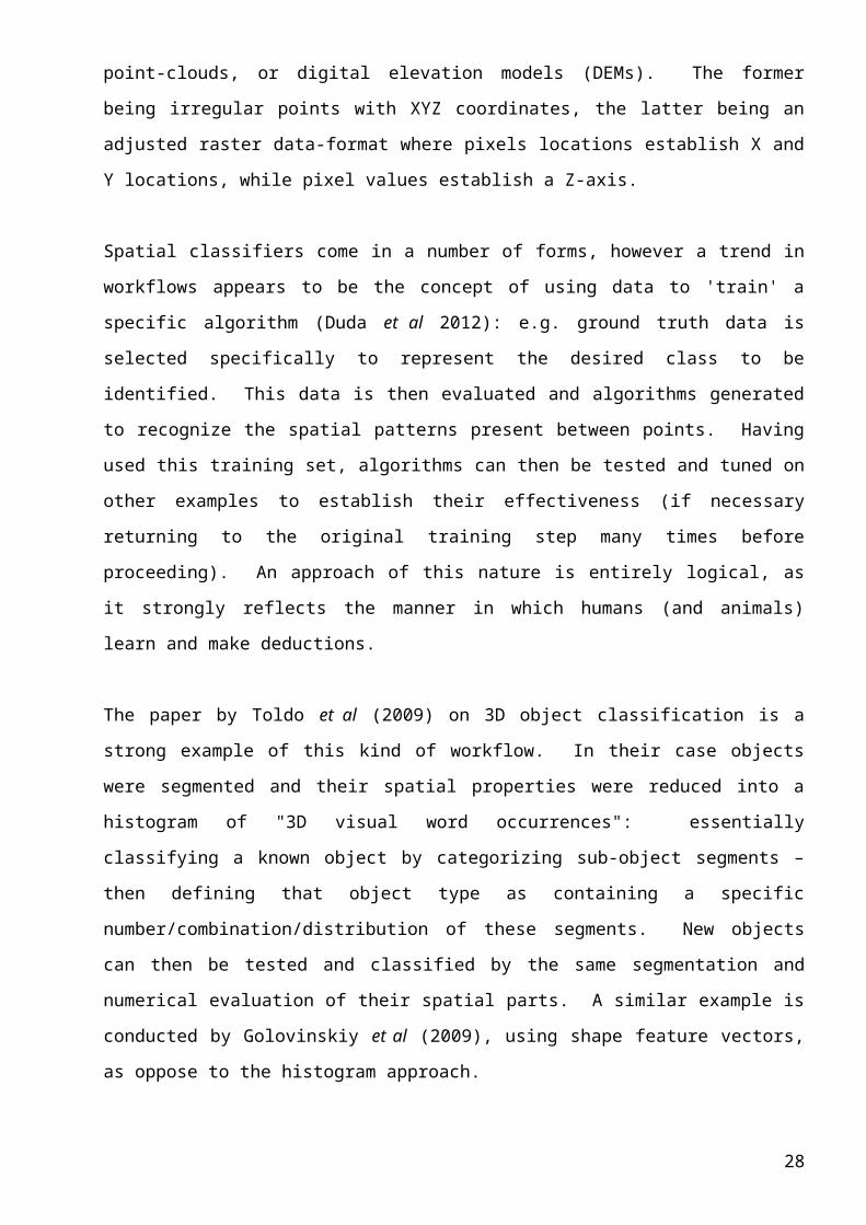
Figure 3.a:

Test Façade data – key: brown = man-made façade objects; green = vegetation; red = unclassified.

28

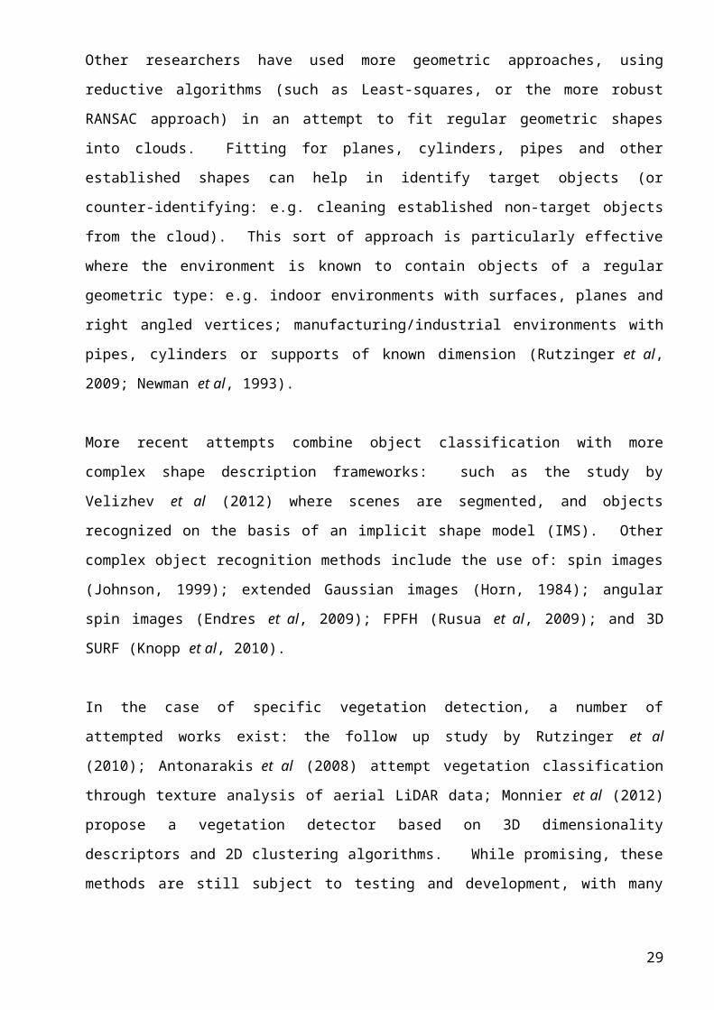
Figure 3.b:

Test Vegetation data – key: brown = man-made façade objects; green = vegetation; red = unclassified.

From this it can be seen the classifier works extremely effectively. The façade test set (figure 3.a)

was particularly effective, with zero false positives, ~96% true-positive and a marginal ~3%

classifier failure rate: this was most likely due to the simple nature of the façade test cloud – as a

predominantly planar example makes for very low geometric complexity or variation. The

vegetation test set was slightly less successful, with a higher classifier failure rate of ~6%, and the

presence of false-positive detection where ~11% of the tree structure was incorrectly identified as

façade objects. Reflecting on this, the classifier still performs highly effectively, with 82.6%

correct detection. At this point it is impossible to make any further quantitative declaration, or

quality assurance, compared to other similar studies (Monnier et al, 2012; Demantké et al 2011;

Hofle et al, 2010), this project lacks a final evaluation against a reliable source of ground-truth data.

Before proving the effectiveness of, or further refining, this algorithm an attempt to evaluate against

a more comprehensive set of reference data must be undertaken.

29

However, a final demonstration of the classifier was performed on the entire scan-tile street scene

(figure 3.c,d – overleaf), and while no statistics are relevant in this instance, it can be qualitatively

seen to be reasonably effective: certainly a platform from which to further refine the classification

scheme.

The issue of false-negatives is difficult to address; while overall the chaotic nature of vegetation

point-clouds does exhibit a predominantly volumetric shape geometry, this chaos can in turn

produce areas which may exhibit planar shape geometry. It can be seen that a larger number of

false-positives were also present in the full test case. Structures such as balconies, window-boxes

and scaffolding mimic the volumetric nature of vegetative branches and leaves.

The obvious solution to these weaknesses is the use of data-fusion methods to exclude planar areas

which list as vegetation objects on other classifiers (e.g. NDVI), and visa-versa, however as this

method is focused on spatial data alone, considering alternatives to data-fusion methods is more

relevant and productive. Monnier et al (2012) suggest the use of a probabilistic relaxation scheme,

to help intelligently classify objects. By weighting the descriptor values of points in relation to

those in the neighbourhood, in an attempt to homogenise cloud areas which form part of the same

object. Another alternative is to use region-growing techniques to progressively classify points

with respect to a second trained rule – which defines the spatial behaviour of vegetation at the

branch, or tree-crown scale. It is possible that particular trained 'object based classification'

schemes mentioned above could also be implemented similarly. Dual spatial detection methods of

this nature could prove to be as effective as data-fusion methods: with multiple steps overcoming

the weaknesses of previous ones, whilst still relying solely on spatial data.

Incidentally, the 'unclassified' areas where this classifier failed appear to correspond to non-planar

regular geometric objects: in particular detecting many cylinders (such as lamp posts and tree

boles) within the scene. This approach could be adapted to adopt an additional specific classifier

class for objects of this nature.

30

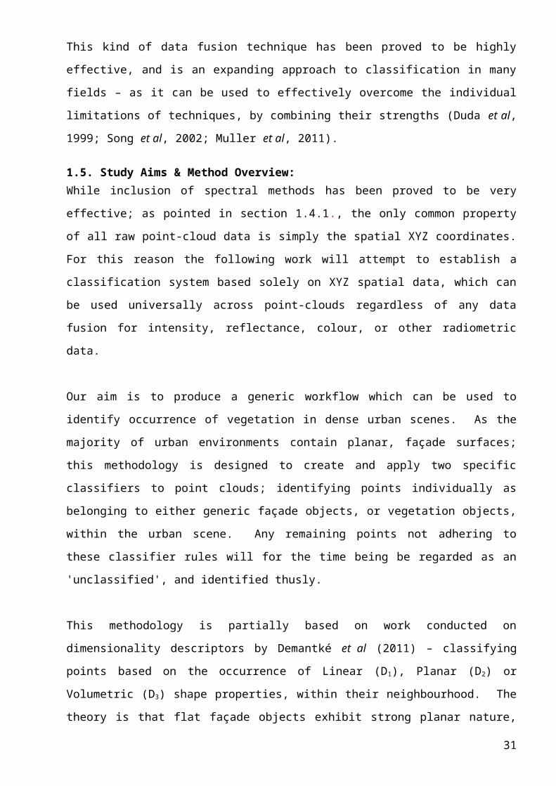
Figure 3.c:

Full Scan-tile view 1 – key: brown = man-made façade objects; green = vegetation; red = unclassified.

Figure 3.d:

Full Scan-tile view 2 – key: brown = man-made façade objects; green = vegetation; red = unclassified.

31

4. Conclusion:

At this point the classifier produced form the workflow here certainly demonstrates potential. It

functions effectively on test sets from a controlled data type (e.g. one that has the same specification

as the training data). Progression of this identifier would certainly include steps to establish

effectiveness across a range of data type/quality. Further examination of the radii selection criteria,

and including automated evaluation of descriptor values would allow this method to function as a

generic workflow. Additionally, the inclusion of a secondary testing phase/quantitative failsafe

would be necessary to consider this a serious classifier.

The work here serves predominantly as a demonstration for the development of pure spatial

classifiers – future studies can branch out from this method and develop and refine more specific

elements of the processing chain: either for their own tailored ends, or with the goal to create an

effective and universal generic spatial classifier.

Auto-Critique:

I originally chose this topic due to my own interest with spatial modelling and identification. I

myself possess an extremely strong spatial awareness – from an early age my family/friends noted

this: from my ability to play racket sports; my comfort reading maps and orientating myself; and

my aptitude at tasks of spatial dexterity (particularly video-games).

Having learned about computer vision in the second term of this masters: I became familiarised

with operators such as the Canny Edge Detector, and the SIFT feature recognition algorithm.

During further reading, I was inspired by the idea that these kinds of operators could be translated

into three dimensional data, for perception and understanding in more complex applications.

Coming from biology and geography backgrounds, I have already done work on vegetation

identification, and the opportunity to develop and test a novel classifier appealed to me. Starting

my background research I quickly found the paper by Monnier et al (2012), which uses the work on

Dimensionality Descriptors by Demantké et al (2011). Immediately this method impressed me with

its simplicity and idealistic goal: of a generic spatial identifier, which may work autonomously on a

variety of point-cloud datasets. At this point I chose to develop my own workflow to further

examine the potential application of these proposed descriptors.

32

The strength of this dissertation is very much stated in its conclusion: the development and

successful performance of the very simple classifier shown here, serves as a platform from which to

expand. A number of attempts have been made to develop specific improvements to this kind of

workflow, it is my hope that the classifier I have developed could serve as an accessible foundation

– from which to systematically include these augmentations.

My perceived weakness of this project is in part the same: the classifier proposed here is very

limited, being simple, reasonably crude, and importantly requiring human intervention to operate. I

would have personally liked to cover more of these potential improvements myself, particularly

refining the code to work as a single fluid function: as it stands I have indicated many of them in the

literature, and left it to future studies to amalgamate their benefits.

In reflection on my work here: the major step that I would have undertaken to improve the study

would be a pre-emptive one. Despite the Scientific Computing module taken in the first term of

this Masters, my background in computer programming is severely lacking. Had I taken more time

to prepare for this specific study, I believe a crash-course (even a self-guided one) in the relevant

language (C++) and software (Microsoft Visual Studio 2010) would have greatly assisted my

productivity: leaving me more time and scope to expand upon the complexity of the classifier, and

not leave the project so open ended. The research and resources do currently exist to make this a

more comprehensive study – I was simply limited by my technical competence when developing

the classifier and was forced to leave much potential to reference of others, or mere speculation.

References:

ABA Surveying ltd. (2013). 3D Scanning & Mobile Mapping. [Online] available at: <

http://www.abasurveying.co.uk/index.htm> [Accessed: August 2013].

Antonarakis, A. S., Richards, K. S., & Brasington, J. (2008). Object-based land cover classification

using airborne LiDAR.  Remote Sensing of Environment, 112(6), pp.2988-2998.

Bayliss, B. (1999). Vegetation survey methods. Max Finlayson & Abbie Spiers, 116.

Bryan, P., Blake, B. and Bedford, J. (2009). Metric Survey Specifications for Cultural Heritage.

Swindon, UK: English Heritage.

Canny, J. (1986). A Computational Approach To Edge Detection. IEEE Trans. Pattern Analysis

and Machine Intelligence, 8(6), pp.679–698.

Defries, R. S. & Townshend, J. R. G. (1994). NDVI-derived land cover classifications at global

scale. International Journal of Remote Sensing 15(17), pp.3567-3586.

Demantké, J., Mallet, C., David, N. and Vallet, B. (2011). Dimensionality based scale selection in

3D LiDAR point clouds, IPRS workshop; laser scanning, volume XXXVIII, Calgary, Canada.

33

Duda, R. O., Hart, P. E., & Stork, D. G. (2012). Pattern classification. Hoboken, NJ, USA: John

Wiley & Sons.

Duda, T., Canty, M., & Klaus, D. (1999). Unsupervised land-use classification of multispectral

satellite images. A comparison of conventional and fuzzy-logic based clustering algorithms.

In: Geoscience and Remote Sensing Symposium, 1999. IGARSS'99 Proceedings. IEEE 1999

International, 2, pp. 1256-1258.

Endres, F., Plagemann, C., Stachniss, C., & Burgard, W. (2009). Unsupervised discovery of object

classes from range data using latent Dirichlet allocation. In Robotics: Science and

Systems, pp. 34.

Exelis Visual Information Studios. (2013). Feature Extraction with Rule-Based Classification

Tutorial. [Online] available at:

<http://www.exelisvis.com/portals/0/pdfs/envi/FXRuleBasedTutorial.pdf> [Accessed: August

2013].

Fernando, R., ed. (2004), GPU Gems: Programming Techniques, Tips and Tricks for Real-Time

Graphics. Boston, USA: Addison-Wesley Professional, for nVIDIA plc.

Food and Agriculture Organization of the United Nations (FAO). (2013). FAOSTAT. [Online]

available at: <http://faostat.fao.org/site/339/default.aspx> [Accessed: August 2013].

Garnaut, R. (2008). The Garnaut Climate Change Review. Cambridge, UK: Cambridge University

Press.

Geodetic Systems Inc. (2013). Geodetic Systems Inc. [Online] available at:

<http://www.geodetic.com/v-stars/what-is-photogrammetry.aspx> [Accessed August, 2013]

Golovinskiy, A., Kim, V. G., & Funkhouser, T. (2009). Shape-based recognition of 3D point clouds

in urban environments. In Computer Vision, 2009 IEEE 12th International Conference on, pp.

2154-2161. IEEE.

HM Government UK. (2012). Building Information Modelling. [Online] available at:

<https://www.gov.uk/government/uploads/system/uploads/attachment_data/file/34710/12-

1327-building-information-modelling.pdf> [Accessed August, 2013].

Horn, B. K. P. (1984). Extended gaussian images. Proceedings of the IEEE,72(12), pp.1671-1686.

Houghton, J. T. ed., Ding, Y. ed., Griggs, D. J. ed., Noguer, M. ed., van der Linden, P. J. ed., Dai,

X. ed., Maskell, K. ed. and Johnson, C. A. ed. (2001). Climate Change 2001: The Scientific

Basis. Cambridge, UK: Cambridge University Press, for the Intergovernmental Panel on

Climate Change (IPCC).

Huete, A., Didan, K., Miura, T., Rodriguez, E. P., Gao, X., and Ferreira, L. G. (2002). Overview of

the radiometric and biophysical performance of the MODIS vegetation indices. Remote

sensing of environment, 83(1), pp.195-213.

Ikeuchi, K. (2001). Modelling from Reality. Dordrecht, Netherlands: Kluwer Academic Publishers

34

Johnson, A. E., & Hebert, M. (1999). Using spin images for efficient object recognition in cluttered

3D scenes. Pattern Analysis and Machine Intelligence, IEEE Transactions on, 21(5), pp.433-

449.

Kanatani, K. (1996). "Statistical Optimization for Geometric Computation", Elsevier Science B. V.

Kedzierski, M., Walczykowski, P., & Fryskowska, A. (2009). Applications of terrestrial laser

scanning in assessment of hydrotechnic objects. In: ASPRS Annual Conference, Baltimore,

Maryland, USA.

Knopp, J., Prasad, M., Willems, G., Timofte, R., & Van Gool, L. (2010). Hough transform and 3D

SURF for robust three dimensional classification. In: Computer Vision–ECCV 2010, pp.589-

602. Springer Berlin Heidelberg.

Monnier, F., Vallet, B., & Soheilian, B. (2012). Trees detection from laser point clouds acquired in

dense urban areas by a mobile mapping system.  ISPRS Annals of the Photogrammetry,

Remote Sensing and Spatial, Information Sciences, I-3, pp.245-250.

Muller, J-P. & Jungrack, K. (2011). Tree and building detection in dense urban environments using

automated processing of IKONOS image and LiDAR data. International Journal of Remote

Sensing 32(8), pp.2245-2273.

NASA. (2012). MODIS Snow / Ice Global Mapping Project. [Online] available at: < http://modis-

snow-ice.gsfc.nasa.gov/>. [Accessed August, 2013].

NASA. (2013). Measuring Vegetation (NDVI & EVI). [Online] available at:

<http://earthobservatory.nasa.gov/Features/MeasuringVegetation/>. [Accessed August, 2013].

Newman, T. S., Flynn, P. J., & Jain, A. K. (1993). Model-based classification of quadric

surfaces. CVGIP: Image Understanding, 58(2), pp.235-249.

Pearce, D. W., & Pearce, C. G. (2001). The value of forest ecosystems. Ecosyst Health, 7(4)

pp.284-296.

Pennsylvania State University. (2013) History of Lidar Development, [Online], available at:

<https://www.e-education.psu.edu/lidar/l1_p4.html> [Accessed August, 2013]

Rottensteiner, F., & Briese, C. (2002). A new method for building extraction in urban areas from

high-resolution LIDAR data.  International Archives of Photogrammetry Remote Sensing and

Spatial Information Sciences, 34(3/A), pp.295-301.

Rutzinger, M., Elberink, S. O., Pu, S., & Vosselman, G. (2009). Automatic extraction of vertical

walls from mobile and airborne laser scanning data. The International Archives of

Photogrammetry, Remote Sensing and Spatial Information Sciences, 38(3), W8.

Rutzinger, M., Pratihast, A. K., Oude Elberink, S., & Vosselman, G. (2010). Detection and

modelling of 3D trees from mobile laser scanning data. International Archives of

Photogrammetry, Remote Sensing and Spatial Information Sciences, 38(5).

35

Song, J. H., Han, S. H., Yu, K. Y., & Kim, Y. I. (2002). Assessing the possibility of land-cover

classification using lidar intensity data. International Archives of Photogrammetry Remote

Sensing and Spatial Information Sciences, 34(3/B), pp.259-262.

Sonka, M., Hlavac, V. and Boyle, R. (2008). Image Processing and Machine Vision. Toronto,

Canada: Thompson.

Sutherland, I. E., Sproull, R. F., & Schumacker, R. A. (1974). A characterization of ten hidden-

surface algorithms. ACM Computing Surveys (CSUR), 6(1), pp.1-55.

Toldo, R., Castellani, U., & Fusiello, A. (2009). A bag of words approach for 3d object

categorization. In Computer Vision/Computer Graphics CollaborationTechniques, pp. 116-

127. Springer Berlin Heidelberg.

United Nations Framework Convention on Climate Change (UNFCCC). (2013a). Kyoto Protocol.

[Online] available at: <http://unfccc.int/kyoto_protocol/items/2830.php> [Accessed: August

2013].

United Nations Framework Convention on Climate Change (UNFCCC). (2013b). Land Use, Land-

Use Change and Forestry (LULUCF). [Online] available at:

<http://unfccc.int/methods/lulucf/items/3060.php> [Accessed: August 2013].

Welsch, R. (1976). Graphics for Data Analysis. Computers & Graphics, 2(1), pp. 31-37.

Wooster, M.J., Zhukov, B. and Oertel, D. (2003). Fire radiative energy for quantitative study of

biomass burning: Derivation from the BIRD experimental satellite and comparison to MODIS

fire products. Remote Sensing of Environment 86, pp.83-107.

Zhang, H., Manocha, D., Hudson, T., & Hoff III, K. E. (1997). Visibility culling using hierarchical

occlusion maps. Proceedings of the 24th annual conference on Computer graphics and

interactive techniques, pp. 77-88. ACM Press/Addison-Wesley Publishing Co..

Appendix:

A.1. PCA; Descriptor; Classifier:#include <pcl/point_types.h>#include <pcl/io/pcd_io.h>#include <pcl/kdtree/kdtree_flann.h>#include <pcl/common/pca.h>

#include <iostream>#include <fstream>#include <list>#include <boost/assign.hpp>

typedef pcl::PointXYZ PointT;

float G (float x, float sigma){ return exp (- (x*x)/(2*sigma*sigma));

36

}

int main (int argc, char *argv[]){ //std::string incloudfile = argv[1]; //std::string outcloudfile = argv[2]; //float sigma_s = atof (argv[3]); //float sigma_r = atof (argv[4]); std::string incloudfile = "in.pcd"; std::string outcloudfile = "out.pcd";

// create cloud pcl::PointCloud<PointT>::Ptr cloud (new pcl::PointCloud<PointT>);

// Set up some counters long count_T = 0; long count_F = 0; long count_U = 0; uint32_t rgb_Ti = ((uint32_t)0) << 16 | ((uint32_t)153) << 8 | ((uint32_t)51); // tree colour: grass green uint32_t rgb_Fi = ((uint32_t)230) << 16 | ((uint32_t)180) << 8 | ((uint32_t)120); // facade colour: pseudo-tan uint32_t rgb_Ui = ((uint32_t)255) << 16 | ((uint32_t)0) << 8 | ((uint32_t)0); // unclassified colour: red float rgb_T = *reinterpret_cast<float*>(&rgb_Ti); float rgb_F = *reinterpret_cast<float*>(&rgb_Fi); float rgb_U = *reinterpret_cast<float*>(&rgb_Ui); float X, Y, Z; std::fstream fin("Point_Cloud.xyz", std::ios_base::in); if(!fin) { std::cout << "failed to open file" << std::endl; return 0; }

while(!fin.eof()) { fin >> X >> Y >> Z; pcl::PointXYZ p(X, Y, Z); cloud->push_back(p); }

fin.close();

// Output Cloud = Input Cloud pcl::PointCloud<PointT> outcloud = *cloud;

int pnumber = (int)cloud->size (); // Set up KDTree pcl::KdTreeFLANN<PointT>::Ptr tree (new pcl::KdTreeFLANN<PointT>); tree->setInputCloud (cloud); //std::fstream out_eigen("F_eigen_log.txt", std::ios::out); //std::fstream out_desc1("F_desc1_log.txt", std::ios::out); //std::fstream out_desc2("F_desc2_log.txt", std::ios::out); //std::fstream out_desc3("F_desc3_log.txt", std::ios::out);

37

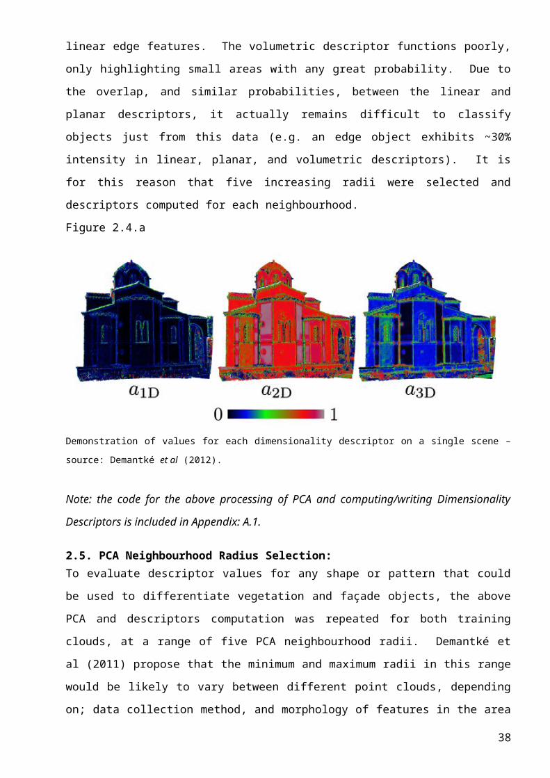
// this is the only output file we actually care about: std::fstream out_Descriptors("Descriptors.txt", std::ios::out); // create a new cloud out: std::fstream out_Cloud_Desc("RGBint.txt", std::ios::out); // create stats out: std::fstream out_Stats("Statistics.txt", std::ios::out); // Main Loop for (int point_id = 0; point_id < pnumber; point_id++) { // set the radius: float radius = 1.5; // Neighbors containers std::vector<int> k_indices; std::vector<float> k_distances;

// later vary radius tree->radiusSearch (point_id, radius, k_indices, k_distances); // k_indices will be the input sub-selection for each PCA ??

Eigen::Vector3f eigen_values; if(k_indices.size()<3) { eigen_values.fill(0.0); } else { // CREATE pca OBJECT! pcl::PCA<PointT> pca; pca.setInputCloud(cloud); // Pass the indices TO pca boost::shared_ptr<std::vector<int> > indicesptr (new std::vector<int> (k_indices)); pca.setIndices (indicesptr); // DO pca eigen_values = pca.getEigenValues(); } if(eigen_values[0] == 0) { float desc1 = 0; float desc2 = 0; float desc3 = 0; out_Descriptors << desc1 << " " << desc2 << " " << desc3 << " "; // Here we start the classification logic: out_Cloud_Desc << rgb_U; count_U++; } else { float desc1 = (eigen_values[0] - eigen_values[1]) / eigen_values[0]; float desc2 = (eigen_values[1] - eigen_values[2]) / eigen_values[0]; float desc3 = eigen_values[2] / eigen_values[0]; out_Descriptors << desc1 << " " << desc2 << " " << desc3 << " "; //std::cout << desc1 << " " << desc2 << " " << desc3 << " ";

38

// Here we start the classification logic: if((desc2 <= 0.6) && (desc3 >= 0.2)) { out_Cloud_Desc << rgb_T; count_T++; } else { if((desc2 >= 0.2) && (desc3 <= 0.2)) { out_Cloud_Desc << rgb_F; count_F++; } else { out_Cloud_Desc << rgb_U; count_U++; } } } //std::cout << count_T << " " << count_F << " " << count_U; //std::cout << "\n"; out_Descriptors << "\n"; out_Cloud_Desc << "\n";

} // main loop // Producing Statistical Results: float Trees_Detected = ((float)count_T/(float)pnumber)*100; float Facade_Detected = ((float)count_F/(float)pnumber)*100; float Point_Unclassified = ((float)count_U/(float)pnumber)*100; float Total_points = (count_T + count_F + count_U); out_Stats << "Tree Detected" << " " << Trees_Detected << "%" << "\n" << "Facade Detected:" << " " << Facade_Detected << "%" << "\n" << "Point Unclassified:" << " " << Point_Unclassified << "%" << "\n" << "Total Points:" << " " << Total_points << "\n"; //out_eigen.close(); //out_desc1.close(); //out_desc2.close(); //out_desc3.close(); // show finish and close out_Descriptor out_Descriptors << "Finished!" << "\n"; out_Descriptors.close(); out_Cloud_Desc.close(); out_Stats.close(); return (0);}

39

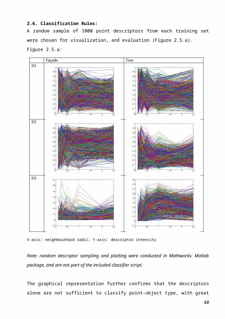
A.2. Read xzy/rbgint; Write .PCD file:#include <iostream>#include <fstream>#include <sstream>#include <string>#include <pcl/io/pcd_io.h>#include <pcl/point_types.h>

using namespace std;

int main(){ int cloud_length = 4448365; // Change this to the "Total Points" in the statistics file int row, col; string line; // character string to hold a single line

pcl::PointCloud<pcl::PointXYZRGB> cloud; // Fill in the cloud data - static allocation// cloud.width = cloud_length;// cloud.height = 1;// cloud.is_dense = false;// cloud.points.resize (cloud.width * cloud.height);

ifstream in_file("Point_Cloud.xyz"); // check default is to open in ascii //, ios::ascii); //Check if the file is open if(in_file.is_open()) // may want to check on skipping whitespace - e.g blank lines? { /* // first check the number of lines in the file and set that to the cloud size cloud_length=0; while(!in_file.eof()) { cloud_length++; cout << cloud_length << "\n"; // this is getting stuck in an infinite loop - why?? } */ if(cloud_length > 0) { cloud.width = cloud_length; cloud.height = 1; cloud.is_dense = false; cloud.points.resize (cloud.width * cloud.height); } else { cout << "XYZ File empty..." << endl; in_file.close(); system("pause"); return (-1); } in_file.seekg(0); // sets input position to zero (equivalent of rewind) //in_file.rewind(); // rewind the file points - may need to check syntax.... cout << "File checked and rewound" << "\n";

row=0; while(!in_file.eof())

40

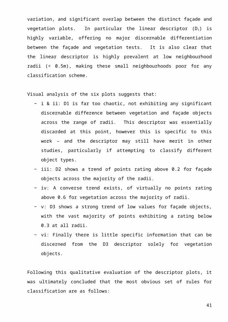
{ // next two lines are critical to decode the multiple data points in each input line getline(in_file, line); // line contains a single line from the file stringstream ss(line); // ss contains a sequence of elements from the the line // cout<<row<<"\n"; // cout<<col<<"\n"; // ideally check if three values in ss (code below assumes that ss automatically increments to the next value in the line) ss >> cloud.points[row].x; ss >> cloud.points[row].y; ss >> cloud.points[row].z; row++; //cout << row << "\n"; } in_file.close();

// could test here that the complete file has been read as row should be equal to cloud_length } else { cout << "XYZ File not opened..." << endl; system("pause"); return (-1); }

// check the contents of "points" for (size_t i = 0; i < cloud.points.size (); ++i) { //cout << cloud.points[i].x << ", " << cloud.points[i].y << ", " << cloud.points[i].z <<'\n'; } // open RGB file ifstream in_file2("RGBint.txt"); // check default is to open in ascii //, ios::ascii); //Check if the file is open if(in_file2.is_open()) {

// might want to also check the number of elements in this file to make sure that there are the same number of RGB values (or at least more!) row=0; while(!in_file2.eof()) // keep going until the end of the file { getline(in_file2, line); // line contains a single line from the file stringstream ss(line); // ss contains a sequence of elements from the the line // cout<<row<<"\n"; // cout<<col<<"\n"; // ideally check if three values in ss (code below assumes that ss automatically increments to the next value in the line) ss >> cloud.points[row].rgb; row++; if(row == cloud.points.size()) { cout << "miss match in number of rgb values\n" << endl; break; // jump out of the file read, but keep going to the next section } } in_file.close();

41

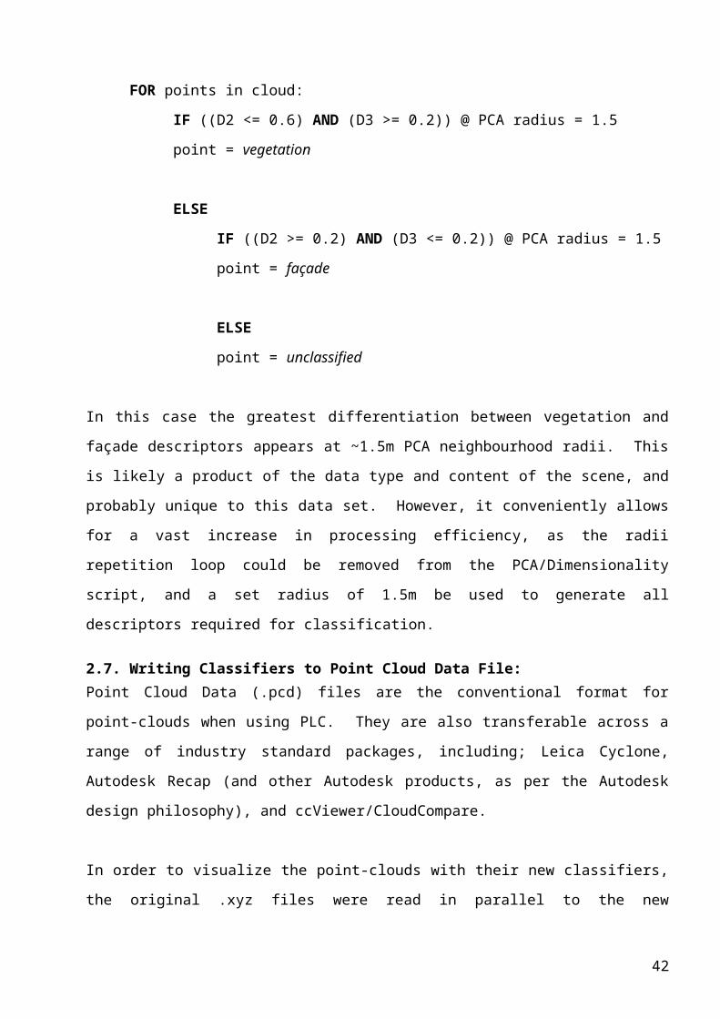
} else { cout << "RGB File not opened..." << endl; system("pause"); return (-1); }

// check the contents of "points" with RGB for (size_t i = 0; i < cloud.points.size (); ++i) { //cout << cloud.points[i].x << ", " << cloud.points[i].y << cloud.points[i].z << cloud.points[i].rgb << '\n'; }

pcl::io::savePCDFileASCII ("TEST_Data_pcd.pcd", cloud); // check the RGB write - but this should give you the xyz at least! std::cerr << "Saved " << cloud.points.size () << " data points to test_pcd.pcd." << std::endl;/* for (size_t i = 0; i < cloud.points.size (); ++i) std::cerr << " " << cloud.points[i].x << " " << cloud.points[i].y << " " << cloud.points[i].z << std::endl;*/ system("pause"); return (0);}

42