Distributions with Fixed Marginals and Related Topics || Isotonic Regression on Permutations

Isotonic Regression on PermutationsAuthor(s): H. W. Block, S. Qian and A. R. SampsonSource: Lecture Notes-Monograph Series, Vol. 28, Distributions with Fixed Marginals andRelated Topics (1996), pp. 45-64Published by: Institute of Mathematical StatisticsStable URL: http://www.jstor.org/stable/4355883 .

Accessed: 10/06/2014 06:01

Your use of the JSTOR archive indicates your acceptance of the Terms & Conditions of Use, available at .http://www.jstor.org/page/info/about/policies/terms.jsp

.JSTOR is a not-for-profit service that helps scholars, researchers, and students discover, use, and build upon a wide range ofcontent in a trusted digital archive. We use information technology and tools to increase productivity and facilitate new formsof scholarship. For more information about JSTOR, please contact [email protected].

.

Institute of Mathematical Statistics is collaborating with JSTOR to digitize, preserve and extend access toLecture Notes-Monograph Series.

http://www.jstor.org

This content downloaded from 194.29.185.112 on Tue, 10 Jun 2014 06:01:10 AMAll use subject to JSTOR Terms and Conditions

http://www.jstor.org/action/showPublisher?publisherCode=ims

http://www.jstor.org/stable/4355883?origin=JSTOR-pdf

http://www.jstor.org/page/info/about/policies/terms.jsp


Distributions with Fixed Marginals and Related Topics IMS Lecture Notes - Monograph Series Vol. 28, 1996

Isotonic Regression on Permutations

By H. W. Block1, S. Qian, and A. R. Sampson1

University of Pittsburgh

Motivated by an approach to qualifying potential judges, we study isotonic

regression problems on a partially ordered set of permutations. We consider the

partial orders discussed in Block, Chhetry, Fang and Sampson (1990) which

are used for comparing the dependence of bivariate empirical distributions with

fixed marginals. We give a method to generate permutations and their inversion

numbers, and develop a technique to input these orders. We discuss methods

of finding predecessors and immediate predecessors in the sense of these orders.

Then, we develop an algorithm to search for isotonic regressions on a set of

permutations under these orders.

1. Introduction and Motivation? This paper presents the algorithms and programs necessary to solve isotonic regression problems involving partial orders on permutations. Our solution depends on some approaches to identi-

fying predecessors for three partial orders given in Block, Chhetry, Fang and

Sampson (1990) and utilizes results of Block, Qian and Sampson (1994) for

computing isotonic regressions over partially ordered sets. The partial orders

of Block et al. (1990) are used for comparing the dependence of bivariate em-

pirical distributions. These distributions have fixed marginals putting mass

1/n at 1,..., ? where ? is the sample size.

One motivation for considering the isotonic regression problem of this

paper is a new approach for qualifying potential judges by utilizing one known

expert's rating of k distinct objects according to some criteria. While we

present the necessary computations for implementing this approach, we do

not present any formal statistical modeling.

Suppose that we wish to evaluate a number of different possible judges who will be expected to rank individuals in a given setting, e.g., wine tastings,

Supported in part by National Security Agency Grant No. MDA-904-90-H-4036 and

in part by National Science Foundation Grant No. DMS-9203444.

AMS 1991 Subject Classification: Primary 62G05; Secondary 20B99

Key words and phrases: Partial orders, permutation, inversion numbers, isotonic

regression.



46 ISO TONIC REGRESSION

athletic competitions or "beauty" contests. To test potential judges, we sup-

pose that we have a single known expert's ranking of k distinct objects from

worst to best according to some qualitative criteria. For example, suppose that

we have a wine expert who provides a rank ordering for the quality of eight 1989 Bordeaux wines from worst to best with no ties permitted. For conve-

nience, we label each wine by its expert ranking, i.e. 1 = worst,..., 8 = best.

The evaluator of the potential judges now picks ? distinct reorderings of the

expert's order (T < 8!). Each of these ? reorderings can be described by the

corresponding permutation. These reorderings are then presented, one at a

time, to a potential judge, who is asked to provide, according to his opinion,

a percentage score for correctness of the presented reorderings. This process

using the ? reorderings is repeated for each of the potential judges.

The evaluator develops the ? reorderings of the expert's evaluation by

following one of three partial orderings on the set of permutations. That is, one

particular partial ordering is selected and the evaluator takes ? reorderings of the expert's ranking according to the rules of the partial ordering. We

now describe in detail how the evaluator would utilize each of these partial

orderings to obtain the ? reorderings.

As an example of our approach, we consider the wine tasting setting.

Initially, the bottles of the eight wines are lined up in the expert's order from

worst (1) to best (8). Then the bottles of wine are moved around according

to the rules of the selected partial order until a reordering is obtained. A

photograph of this reordering is taken and this is one of the ? reorderings

presented to the subject. This process is repeated to obtain the other ? ? 1

reorderings. Each of these photographs is then presented to a potential judge

who is told that this is a ranking from worst to best (physically ordered from

left to right) and is asked to give a grade for how good this ranking is. If the

judge has good ability, we would expect high scores to be given to rankings

similar to the expert's rankings and low scores to those which are quite different

from the expert's ranking. Moreover, if one ordering is "closer" to the experts

order than another, then the former score should be higher than the latter.

We now describe the three partial orders (designated b\,b2 or 63) which

would be used to obtain the reorderings. The oi ordering involves a finite

sequence of switches, where the evaluator may switch out of order any two

wine bottles among the eight, which are in the expert's original order, (e.g.,

(13546278) may be switched to (13546872)). The second ordering, the b2

ordering, only permits the evaluator to sequentially switch wine bottles which

were originally adjacent in the expert's original order (e.g., (13546278) may

be switched to (13547268)). This allows for the reordering of the wine where

changes are very subtle, and is of use in discerning a potential judge's ability to



H. W. BLOCK, S. QIAN, A. R. SAMPSON 47

make fine discriminations. The third (63) ordering that we consider permits the

evaluator to sequentially switch neighboring bottles out of the expert's order

(e.g., (13546278) can be switched to (13564278)). This latter ordering can

be viewed as an ordering for switching convenience, i.e., moving neighboring

bottles. A more rigorous treatment of these three partial orderings can be

found in Block, Chhetry, Fang and Sampson (1990).

Let i and j be two of the evaluator's ? reorderings which were arranged

according to one of the three orderings 61,62 or 63. A potential judge will be

in concordance with the expert according to a particular partial ordering if i

is better ordered than j implies that the potential judge scores the ordering i

at least as high as that of j. Note that i is better ordered than j if i is in some

sense closer to the expert's rating than is j, according to that partial order.

If the evaluator has chosen many test permutations, then it is unrealistic

to expect the potential judge to be in perfect concordance with all these per-

mutations with respect to the fixed partial ordering under consideration. To

measure each potential judge's degree of discrepancy, we use the measure

min J>(i)

- /(i))2

where the sum is over all ? permutations and the minimum is taken over all

functions / which are isotonic with respect to the ordering, that is, i better

ordered than j implies /(i) > /(j), and where s(i) is the potential judge's score for permutation i subject to s(i) being constrained in some way so that

the scores are comparable across potential judges. From this measure, we

can see how far the potential judge is from the closest scoring which is in

perfect concordance with the given ordering. To compute this measure, we

need to find the isotonic regression of the judge's score function on the set of

? given permutations with respect to the selected partial order. One could

then use this measure, computed for each judge, to decide if each judge should

be qualified or not.

We note that we motivate and apply our results in the context of quali-

fying judges. However, in the spirit of Block et al. (1990) one could consider

any function defined on the set of bivariate empirical rank distributions and

one of the four orderings for positive dependence and then isotonize that func-

tion with respect to the given ordering. Our methods would apply to such a

problem.

In Section 2, we formulate the problem and in Section 3 study methods

of finding an immediate predecessor of a permutation in Sn with respect to

certain partial orders. Sections 4 and 5 prove further computational details.

In Section 6 specific computations are given for various choices of the function

s. The program for our algorithm is given in the Appendix.




2. Problem Formulation. Let Sn be the set of all permutations of the

? integers {l,2,...,n}. Partial orders on Sn have been studied in statistics,

computer science, discrete mathematics and other areas. Block, Chhetry, Fang and Sampson (henceforth BCFS) (1990) gave a unified approach to three well

known partial orders on Sn and introduced a new one. They called these partial

orders the 6i, 62, 63 and 64 orders. BCFS (1990) showed that the 6i, 62,63 and 64

orders correspond to the more concordant, more row regression, more column

regression and more associated orders on the class of bivariate empirical rank

distributions, respectively. While our motivation was based on the three orders

61,62 and 63, we include results for 64 for completeness.

Let i = (?1, ?2,.. ?, in) ? Sn. An inversion of i is a pair of indices (k,l) of i with k < I and ik > ih An inversion (k,l) of i is said to be of type 2

if ik ? %i = 1. An inversion (k,l) of i is said to be of type 3 if / = k + 1,

i.e., ik and ?/ are adjacent elements in the permutation. The inversion number

of a permutation i is the number of inversions contained in i, and is denoted

as ra(i). It is well known that 0 < ra(i) < n(n -

l)/2, for any i ? Sn. An

interchange of two components ik and i\ of a permutation i is said to be a

correction if (k,l) is an inversion of i.

A permutation i is said to be better ordered than j in the sense of 61-

order, written as i >i j, if i = j or i is obtainable from j in a finite number of

steps, each of which consists of a correction of an inversion. A permutation i

is said to be better ordered than j in the sense of 62-order, written as i >2 j,

if i = j or i is obtainable from j in a finite number of steps, each of which

consists of interchanging an inversion of type 2. A permutation i is said to be

better ordered than j in the sense of 63-order, written as i >3 j, if i = j or i is

obtainable from j in a finite number of steps, each of which consists of inter-

changing an inversion of type 3. A permutation i is said to be better ordered

than j in the sense of 64-order, written as i >4 j, if i = j or i is obtainable

from j in a finite number of steps, each of which consists of interchanging an

inversion of type 2 or type 3.

BCFS (Theorem 2.5, 1990) showed that the 62- and 63-orders are not

equivalent and each implies the 64-order; and that the 64-order implies the

61-order.

A real valued function / on Sn is said to be isotonic with respect to a

6?-order, if /(i) > /(j), whenever i >t j, where t = 1,2,3 or 4. The class of

all isotonic functions on Sn with respect to a 6rorder is denoted as It. A real

valued function s* on Sn is said to be an isotonic regression of a given function

s with nonnegative weights w, if s* is the solution of the following problem:




min ^2(s(x)- f(x))2w(x) subject to f e It. (2.1)

x?Sn

For any given function s on Sn with positive weights w(-), the objective

functional is continuous and strictly convex. Hence, there exists a unique

isotonic regression of s with weights w.

Problems of the form (2.1) are called isotonic regression problems on the

set of permutations subject to the 6?-orders. These problems can arise in the

evaluation of ranking problems and evaluating disorder in computer sorting

algorithms. A comprehensive reference for isotonic regression is Robertson,

Wright and Dykstra (1988). Recently, Block, Qian and Sampson (henceforth,

BQS) (1992, 1994) gave a unified approach to a wide class of algorithms for

isotonic regressions and developed some new efficient algorithms, especially

for partial orders.

A partial order on a finite set X can be represented as a directed graph without cycles, but this representation is not unique. The representation with

a minimum number of edges is called a Hasse diagram. In this diagram, each

edge is a pair of elements in X such that one of them is an immediate prede-

cessor of the other. The advantage of this representation is that the depiction of the partial order is compact and easy to handle. Additionally, in compu-

tation, this representation saves a significant amount of computer memory.

Consequently, it is commonly used in algorithms for partial orders. The IBCR

algorithm developed by BQS (1994), which searches for an isotonic regression on a partially ordered set is able to use this representation to facilitate the

computation of various partial orders. In order to utilize this representation, we must know all immediate predecessors of each element in X. Therefore, it

is basic to find the immediate predecessors of each element in Sn, in order to

apply the IBCR algorithm to problem (2.1).

3. Immediate Predecessors Under the 6?-Orders. In this section

we study methods for finding immediate predecessors of permutations in Sn with respect to the 6rorders.

Let t = 1,2,3 or 4, and let j,i ? Sn. The permutation i is said to be a

predecessor of j in the sense of 6rorder, if j >t i and j f i; the permutation k is said to be an immediate predecessor of j in the sense of 6?-order, if k is

a predecessor of j and no permutation is between k and j in the sense of the

same 6rorder. Recall that m(i) is the inversion number of the permutation i.

Lemma 3.1. Let i be a predecessor of j in Sn in the sense ofbt-order with

t e {1,2,3,4}. Then ra(i) > m(j).




Proof. When j is obtained from i by correcting an inversion, it is well

known that ra(i) > m(j). If i is a predecessor of j in the sense of 6i-order, by

transitivity, we have m(i) > m(j). The proposition is true for other 6rorders, because each of them implies the 61-order. |

Corollary 3.2. Let t = 1,2,3 or 4, and let i be a predecessor of] in Sn

in the sense ofbt-order. Then m(i) ?

ra(j) = 1 implies that i is an immediate

predecessor of} in the sense of the bt-order.

Lemma 3.3. If i is an immediate predecessor of j in Sn in the sense of one

of the bt-orders, then j is obtained from i by a correction of an inversion.

Lemma 3.4. A permutation j is obtained from a permutation i by a

correction of an inversion if and only if m(i) > m(j) and i and j differ by

exactly two different components.

Proof. The necessity of the condition is proved by Lemma 3.1. If i and

j differ by exactly two different components, k and /, then j is obtained from

i by interchanging the k-th and /-th components of i. Since ra(i) > m(j), we

have (k -

l)(ik ?

ii) < 0. Hence, j is obtained from i by a correction of an

inversion (k,l). I

Lemma 3.5. Let j be obtained from i by interchanging the k-th and l-th

components of i with k < I and ik > ii, i.e., j is obtained from i by a correction

of an inversion. If for each index u between k and I, iu > ik, or iu < i?, then

m(i) -

ra(j) = 1.

Proof. Assume for u between k and / that iu > ik. Since iu > ik > i/,iu

is responsible for only one inversion with respect to ik and ?/ in i. Similarly

in j,?/ and iu are ordered, and iu and ik are disordered, so ik causes only one

inversion in j. If iu < i\, the argument is similar. Consequently the net change

from i to j is one, i.e., the correction of the inversion in the k and / positions.

I

Corollary 3.6.

(1) Jf j is obtained from i by a correction of an inversion of type 2, then

m(i) -

m(j) = 1;

(2) Jf j is obtained from i by a correction of an inversion of type 3, then

m(i) -

ra(j) = 1.

Theorem 3.7. A permutation i is an immediate predecessor of a permu-

tation j in the sense ofb\-order on Sn, if and only if,

(1) m(i) ?

m(j) = 1; and

(2) there are exactly two different components between i and j.




Proof. Sufficiency follows from Corollary 3.2. Let i be an immediate

predecessor of j. By Lemma 3.3, j is obtained from i by a correction of an

inversion. Hence, by Lemma 3.4, m(i) > ra(j) and (2) is satisfied. Assume

there exists an index u between the two different components k and / with

k < I, otherwise ra(i) ?

m(j) = 1. Now we assume ra(i) ?

ra(j) > 1. By

Lemma 3.5, ?/ < iu < ik? Let j1 be obtained by interchanging fc-th and u-

th components of j? = i; let j2 be obtained by interchanging u-th. and /-th

components of j1; then j3 = j is obtained by interchanging k-th and u-th.

components of j2. Because i\ < iu < ik, each j* is obtained from jt_1 by a

correction of an inversion. Thus j1 and j2 are between i and j in the sense of

6i-order. This contradicts i being an immediate predecessor of j. |

If we know the inversion numbers for all permutations in Sn, we can easily find all immediate predecessors for each element in Sn in the sense of the 6i-

order by Theorem 3.7. For any permutation j, each immediate predecessor of

j has inversion number ra(j) + 1. If a permutation with the inversion number

(ra(j) + 1) has exactly two different components from the permutation j, it is

an immediate predecessor of j. All immediate predecessors of j in the sense of

the 6i-order can be found in this way. Conditions 1) and 2) in Theorem 3.7

can be easily implemented in a program.

For 62,63 and 64 orders, we have similar theorems for their immediate

predecessors. We summarize the results below.

Theorem 3.8. (a) Fort = 2,3,4, a permutation i is an immediate predecessor of a permutation j in the sense of the bt-order on Sn if and only if j is

obtained from i by a correction of an inversion of type t.

(b) Necessary and sufficient conditions for i to be an immediate predecessor of} are:

(1) m(i) -

m(j) = 1;

(2) i and j differ in exactly two components;

(3) for the two components k and I of 2);

\ik ?

i/| = 1 (f?r b2-orderings) ,

\k ?

l\ = 1 (for bs-orderings) ,

\ik -

t/| = 1 , or \k -

l\ = 1 (for b4-orderings) .

4. Generating the Elements of Sn and Their Inversion Numbers.

From Section 3, it is clear that the inversion numbers of the permutations play



5 2 ISO TONIC REGRESSION

an important role in searching for immediate predecessors of an element in Sn

in the sense of 6rorders. The inversion number of a permutation can be

computed by its definition, but we develop in this section an efficient way of

finding the inversion numbers for all elements in Sn, utilizing the structure of

Sn. While there are many algorithms to generate permutations we know of

none to find inversion numbers. The set of permutations, Sn, has n! elements,

and the range of the inversion numbers for i ? Sn is {0,1,...,6} with 6 =

n(n ?

l)/2. We begin by using the inversion numbers to divide Sn into 6+1

subsets. The subset containing all the permutations with inversion number

u is called the u-th layer of Sn and is denoted as SUyU. For example, for

S2 = {(12),(2 1)},{(12)} is the 0-th layer and {(2 1)} is the 1st layer of S2.

We use a recursive method to generate Sn from 5n_i, where a = (n -

l)(n -

2)/2 is the maximal inversion number of 5?-?? Assume that we have

obtained 5n-i with layers 5n_i,o, 5n-i,i,..., 5?_??a, and assume the k-th layer

Sn-i,k has wn_\yk elements. For each permutation i in Sn, we can view i as

obtained by inserting the integer ? into a permutation j of order (n - 1).

For each permutation j = (j\, j2,... ,jn-\), there are ? locations available for

inserting the integer n. Let h be an integer between 1 and n. We define an

inserting function f^ on Sn-\ to Sn as follows:

<t>htt) - (Ji<>--Jh-i,n,jh,? ? -,jn-l) .

Let A be a subset of Sn, and <t>h(A) denote the range of </>h on A. Obviously

the function f^ is a one to one correspondence from 5n_i onto f?(3?-?) =

{i ? Sn : ih ? ?). The set Sn is a union of </>/?(5?_?),? = 1,2,..., ?, i.e.,

5? = ?{0?(5?-?):? = 1,2,...,?}.

Theorem 4.1. Let h be an integer between 1 and ? inclusive, and let

j E Sn-i? Then

?(<MJ)) = ?(J) + (n-h) .

Proof. The function f^ inserts ? into the h-th location of j, which

generates ? ? h inversions for integer n, and the inversions of other integers

do not change after the insertion. Hence, m(</>^(j)) = ra(j) + (n ?

h). |

Corollary 4.2. Let wUiX be the numbers of elements in SnjX, the x-th

layer of Sn and a = (n -

l)(n ?

2)/2.

(1) For ? = 0,1,. ..,n- 1,

Sn,x = <f>n(Sn-l,x) U f?-\ (Sn-\,x-\ ) U . . . U f?-?(3?-??), and

Wn,x = Wn-iyX + Wn-iiX-i + . . . + Wn-1,0 ?




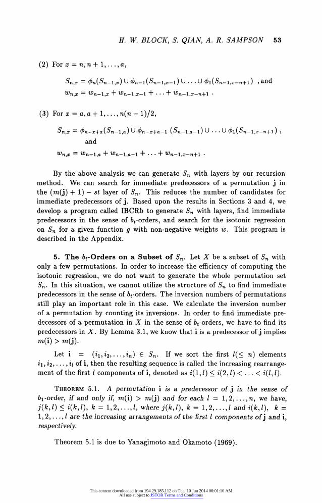
(2) For x = ?, n + 1,..., a,

Sn,x = <l>n(Sn-l,x) U </>n-l(?n-l,:r-l) U . . .U 0l(5n-lfa?-n+l) , and

Wn,tf = ?p-1,? + ^n-l,x-l + ? ? ? + ^?-?,?-?+? .

(3) For a: = a, a + 1,..., n(n ?

l)/2,

Sn,x = <??-2?-a(??-1,a) U <??-?+a-1 (??-?,a-?) U . . . U ^(S^-i^-n+i ) ,

and

?n,x = ?^?-?,a + Wn-l,a-l + ? ? ? + Wn-?,?-?+? ?

By the above analysis we can generate Sn with layers by our recursion

method. We can search for immediate predecessors of a permutation j in

the (m(j) + 1) ? st layer of Sn. This reduces the number of candidates for

immediate predecessors of j. Based upon the results in Sections 3 and 4, we

develop a program called IBCRb to generate Sn with layers, find immediate

predecessors in the sense of 6rorders, and search for the isotonic regression on Sn for a given function g with non-negative weights w. This program is

described in the Appendix.

5. The 6<-Orders on a Subset of Sn. Let X be a subset of Sn with

only a few permutations. In order to increase the efficiency of computing the

isotonic regression, we do not want to generate the whole permutation set

5n. In this situation, we cannot utilize the structure of Sn to find immediate

predecessors in the sense of 6rorders. The inversion numbers of permutations

still play an important role in this case. We calculate the inversion number

of a permutation by counting its inversions. In order to find immediate predecessors of a permutation in X in the sense of 6rorders, we have to find its

predecessors in X. By Lemma 3.1, we know that i is a predecessor of j implies

m(i) > m(j).

Let i = (?i,?2i ? - -??n) ? Sn. If we sort the first /(< n) elements

?i, i2,..., ii of i, then the resulting sequence is called the increasing rearrange- ment of the first / components of i, denoted as ?(1, /) < ?(2, /)<...< i(l, I).

Theorem 5.1. A permutation i is a predecessor of j in the sense of

bi-order, if and only if, m(i) > ra(j) and for each I = 1,2, ...,n, we have,

j(k, I) < i(k, 1), k = 1,2,...,/, where j(k, I), k = 1,2,...,/ and i(k, I), k =

1,2,...,/ are the increasing arrangements of the first I components of} and i,

respectively.

Theorem 5.1 is due to Yanagimoto and Okamoto (1969).



54 ISOTONIC REGRESSION

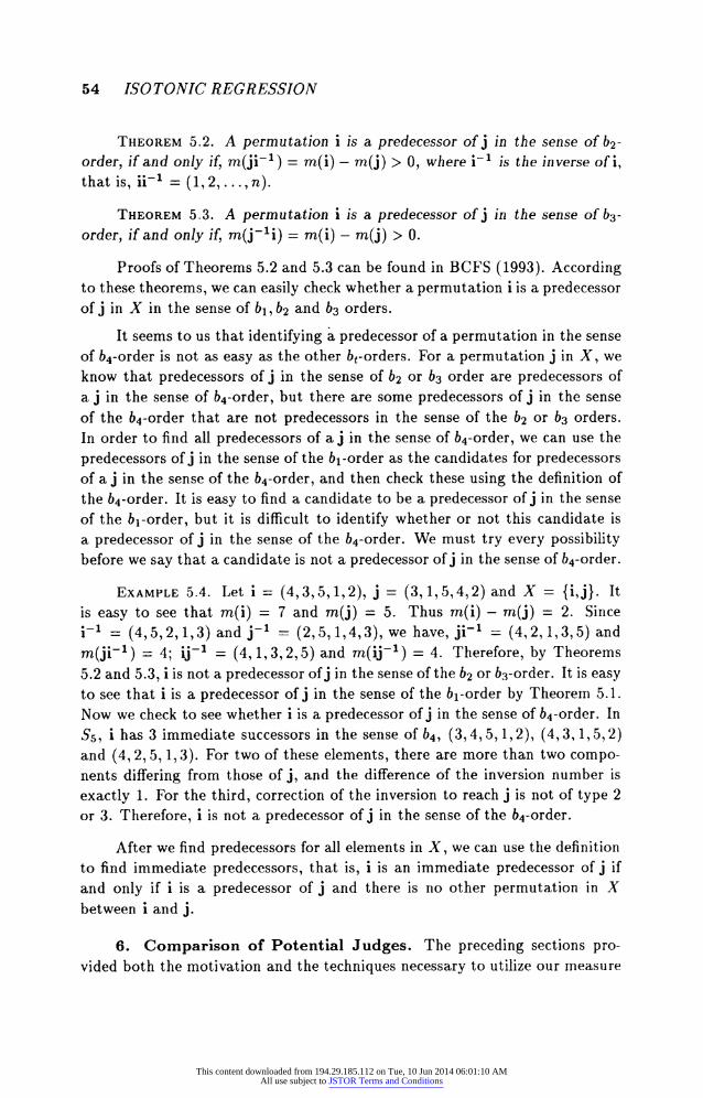
Theorem 5.2. A permutation i is a predecessor of} in the sense of b2-

order, if and only if, ra(ji_1) = ra(i) -

ra(j) > 0, where i**"1 is the inverse of i,

that is, ii-1 = (1,2,.. .,n).

Theorem 5.3. A permutation i is a predecessor of} in the sense of 63-

order, if and only if, ra(j_1i) = ra(i) -

ra(j) > 0.

Proofs of Theorems 5.2 and 5.3 can be found in BCFS (1993). According to these theorems, we can easily check whether a permutation i is a predecessor

of j in X in the sense of 61,62 and 63 orders.

It seems to us that identifying a predecessor of a permutation in the sense

of 64-order is not as easy as the other 6rorders. For a permutation j in X, we

know that predecessors of j in the sense of 62 or 63 order are predecessors of

a j in the sense of 64-order, but there are some predecessors of j in the sense

of the 64-order that are not predecessors in the sense of the 62 or 63 orders.

In order to find all predecessors of a j in the sense of 64-order, we can use the

predecessors of j in the sense of the 61-order as the candidates for predecessors

of a j in the sense of the 64-order, and then check these using the definition of

the 64-order. It is easy to find a candidate to be a predecessor of j in the sense

of the 61-order, but it is difficult to identify whether or not this candidate is

a predecessor of j in the sense of the 64-order. We must try every possibility

before we say that a candidate is not a predecessor of j in the sense of 64-order.

Example 5.4. Let i = (4,3,5,1,2), j = (3,1,5,4,2) and X = {i,j}. It

is easy to see that m(i) = 7 and m(}) = 5. Thus ra(i) -

ra(j) = 2. Since

i"1 = (4,5,2,1,3) and j"1 = (2,5,1,4,3), we have, ji"1 = (4,2,1,3,5) and

m(}i~1) = 4; ij_1 = (4,1,3,2,5) and ra(ij_1) = 4. Therefore, by Theorems

5.2 and 5.3, i is not a predecessor of j in the sense of the 62 or 63-order. It is easy

to see that i is a predecessor of j in the sense of the 61-order by Theorem 5.1.

Now we check to see whether i is a predecessor of j in the sense of 64-order. In

Ss, i has 3 immediate successors in the sense of 64, (3,4,5,1,2), (4,3,1,5,2)

and (4,2,5,1,3). For two of these elements, there are more than two compo-

nents differing from those of j, and the difference of the inversion number is

exactly 1. For the third, correction of the inversion to reach j is not of type 2

or 3. Therefore, i is not a predecessor of j in the sense of the 64-order.

After we find predecessors for all elements in X, we can use the definition

to find immediate predecessors, that is, i is an immediate predecessor of j if

and only if i is a predecessor of j and there is no other permutation in X

between i and j.

6. Comparison of Potential Judges. The preceding sections pro-

vided both the motivation and the techniques necessary to utilize our measure




of discrepancy to evaluate a potential judge. However, as noted in Section 2, to

compare two or more potential judges by the proposed measure of discrepancy,

we need to provide some type of constraints on the scores that the potential

judges may utilize. The reason for this is that the measure of discrepancy is

sensitive to the scaling that the potential judges would be using in assigning

their scores, s(i). For instance, two judges assigning scores in the same order

pattern, but with one using a narrow range of scores and the other using a

large range of scores, would have different degrees of discrepancies although

their scores would have the same order pattern. There are several techniques

for standardizing the scores to take into account the variability of the po-

tential judges' scores. In the example presented in this section, we consider

the following approach in order to avoid this scaling problem. When asking

a potential judge to assign scores to ? orderings, we require that the judge

use one of ? scores pre-specified by the evaluator. Furthermore, once one of

these pre-specified scores is used by a potential judge that score is removed

from further possible usage by that judge. In application, the judge would be

given a box of ? chips with percentages marked on the chips and the judge

would pick and assign one of these chips to each of the presented ? orderings.

Moreover, we would allow the judge to see all ? orderings before assigning the

prescribed scores.

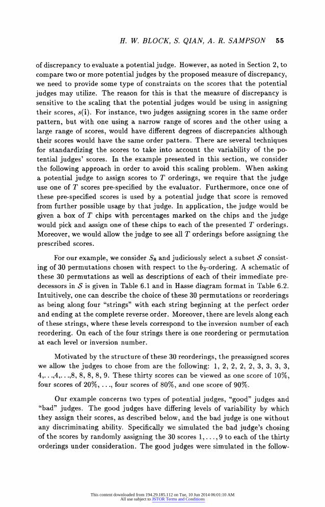
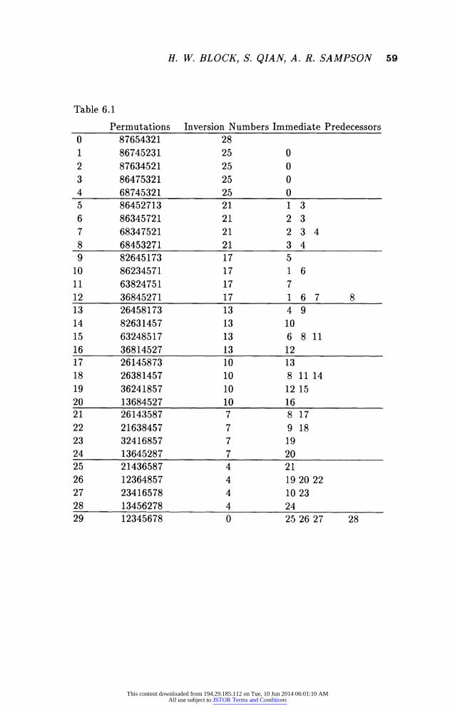
For our example, we consider 5s and judiciously select a subset S consist-

ing of 30 permutations chosen with respect to the 63-ordering. A schematic of

these 30 permutations as well as descriptions of each of their immediate pre-

decessors in S is given in Table 6.1 and in Hasse diagram format in Table 6.2.

Intuitively, one can describe the choice of these 30 permutations or reorderings as being along four "strings" with each string beginning at the perfect order

and ending at the complete reverse order. Moreover, there are levels along each

of these strings, where these levels correspond to the inversion number of each

reordering. On each of the four strings there is one reordering or permutation at each level or inversion number.

Motivated by the structure of these 30 reorderings, the preassigned scores

we allow the judges to chose from are the following: 1, 2, 2, 2, 2, 3, 3, 3, 3,

4,.. .,4,.. .,8, 8, 8, 8, 9. These thirty scores can be viewed as one score of 10%, four scores of 20%, ..., four scores of 80%, and one score of 90%.

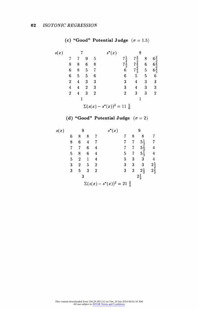
Our example concerns two types of potential judges, "good" judges and

"bad" judges. The good judges have differing levels of variability by which

they assign their scores, as described below, and the bad judge is one without

any discriminating ability. Specifically we simulated the bad judge's chosing of the scores by randomly assigning the 30 scores 1,..., 9 to each of the thirty

orderings under consideration. The good judges were simulated in the follow-




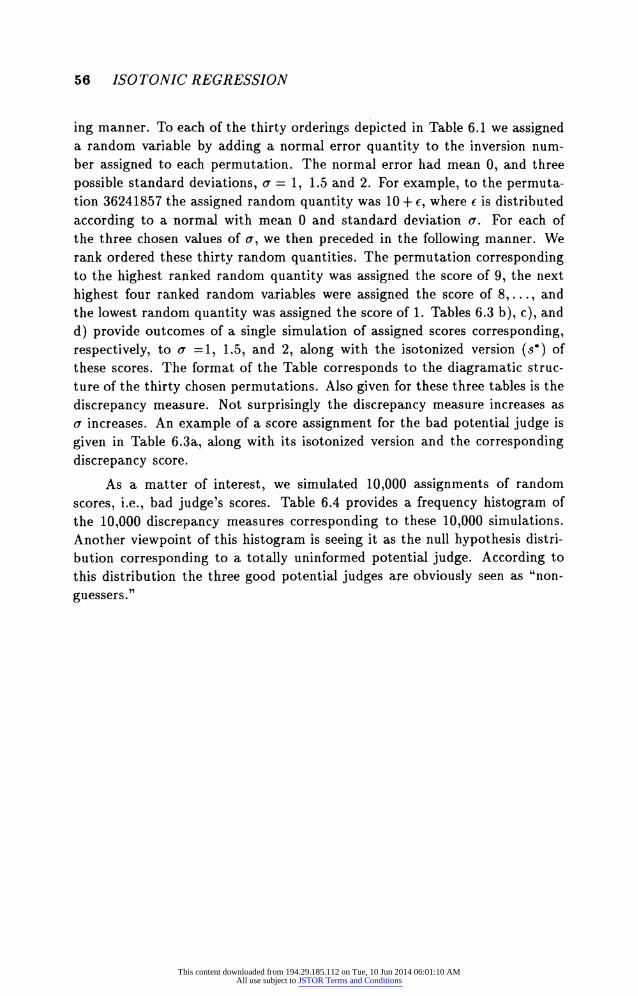
ing manner. To each of the thirty orderings depicted in Table 6.1 we assigned a random variable by adding a normal error quantity to the inversion num-

ber assigned to each permutation. The normal error had mean 0, and three

possible standard deviations, s = 1, 1.5 and 2. For example, to the permuta-

tion 36241857 the assigned random quantity was 10 + e, where e is distributed

according to a normal with mean 0 and standard deviation s. For each of

the three chosen values of s, we then preceded in the following manner. We

rank ordered these thirty random quantities. The permutation corresponding

to the highest ranked random quantity was assigned the score of 9, the next

highest four ranked random variables were assigned the score of 8,..., and

the lowest random quantity was assigned the score of 1. Tables 6.3 b), c), and

d) provide outcomes of a single simulation of assigned scores corresponding,

respectively, to s =1, 1.5, and 2, along with the isotonized version (s*) of

these scores. The format of the Table corresponds to the diagramatic struc-

ture of the thirty chosen permutations. Also given for these three tables is the

discrepancy measure. Not surprisingly the discrepancy measure increases as

s increases. An example of a score assignment for the bad potential judge is

given in Table 6.3a, along with its isotonized version and the corresponding

discrepancy score.

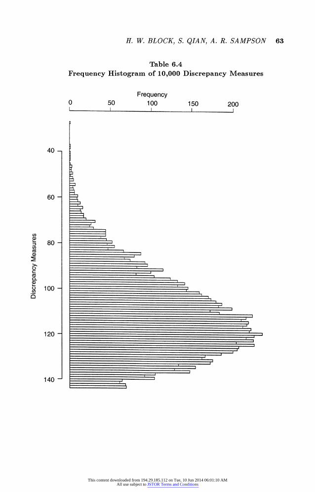
As a matter of interest, we simulated 10,000 assignments of random

scores, i.e., bad judge's scores. Table 6.4 provides a frequency histogram of

the 10,000 discrepancy measures corresponding to these 10,000 simulations.

Another viewpoint of this histogram is seeing it as the null hypothesis distri-

bution corresponding to a totally uninformed potential judge. According to

this distribution the three good potential judges are obviously seen as "non-

guessers."




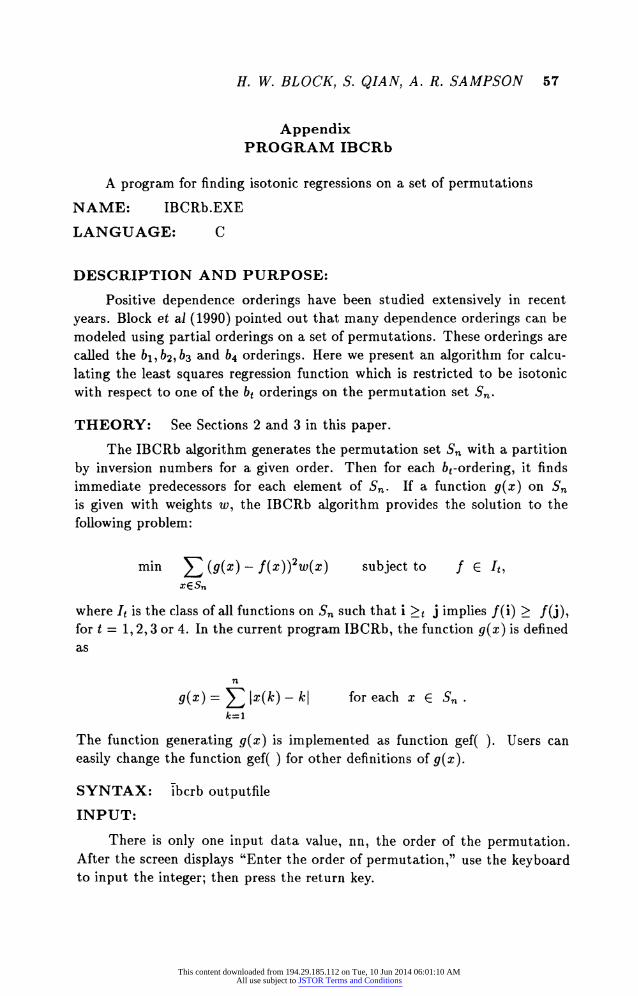
Appendix

PROGRAM IBCRb

A program for finding isotonic regressions on a set of permutations

NAME: IBCRb.EXE

LANGUAGE: C

DESCRIPTION AND PURPOSE:

Positive dependence orderings have been studied extensively in recent

years. Block et al (1990) pointed out that many dependence orderings can be

modeled using partial orderings on a set of permutations. These orderings are

called the 61,62,63 and 64 orderings. Here we present an algorithm for calcu-

lating the least squares regression function which is restricted to be isotonic

with respect to one of the bt orderings on the permutation set Sn.

THEORY: See Sections 2 and 3 in this paper.

The IBCRb algorithm generates the permutation set Sn with a partition

by inversion numbers for a given order. Then for each 6rordering, it finds

immediate predecessors for each element of Sn. If a function g(x) on Sn

is given with weights w, the IBCRb algorithm provides the solution to the

following problem:

min 2Z (q(x) ~-

f(x))2w(x) subject to / G It,

x?Sn

where It is the class of all functions on Sn such that i >t j implies /(i) > /(j), for t = 1,2,3 or 4. In the current program IBCRb, the function g(x) is defined

as

g(x) = 2^ \x(k)

? k\ for each x G Sn .

fc=l

The function generating g(x) is implemented as function gef( ). Users can

easily change the function gef( ) for other definitions of g(x).

SYNTAX: ?bcrb outputfile

INPUT:

There is only one input data value, nn, the order of the permutation. After the screen displays "Enter the order of permutation," use the keyboard to input the integer; then press the return key.




SCREEN OUTPUT:

After entering the order of the permutations, "The order of permutations is nn." is displayed on the screen.

After finishing the calculation of the four isotonic regressions, it prints

"Success." on the screen.

FILE OUTPUT:

1. Accumulation number of elements in each level.

2. The permutations with codes in each level.

3. Four tables. Each table is for a 6rordering, and has more than 4 columns.

Column 1: code of each permutation;

Column 2: the original function g(x);

Column 3: the weight functions w(x);

Column 4: the isotonic regression g*(x) of g with weights w;

Column 5 and up: the codes of immediate predecessors of each per-

mutation.




Table 6.1

_Permutations Inversion Numbers Immediate Predecessors

~? 87654321 28

1 86745231 25 0

2 87634521 25 0

3 86475321 25 0

_4_68745321_25_0_ 5 86452713 21 1 3

6 86345721 21 2 3

7 68347521 21 2 3 4

_8_68453271_21_3_J_ 9 82645173 17 5

10 86234571 17 1 6

11 63824751 17 7

12_36845271_17_16 7 8

13 26458173 13 4 9

14 82631457 13 10

15 63248517 13 6 8 11

16_36814527_13_12_ 17 26145873 10 13

18 26381457 10 8 11 14

19 36241857 10 12 15

20_13684527_10_16_ 21 26143587 7 8 17

22 21638457 7 9 18

23 32416857 7 19

24_13645287_7_20_ 25 21436587 4 21

26 12364857 4 19 20 22

27 23416578 4 10 23

28_13456278_4_24_ 29 12345678 0 25 26 27 28




Table 6.2

Hasse Diagram Corresponding To Table 6.1

(29)12345678

12364857.

21436587 (25)

26143587(21)

26145873(17)

26458173(13)

82645173 (9)

86452713 (5) T*^-^Ur?nre-?r

86745231 (1)

127)23416578

(23)32416857

(19)36241857

115)63248517

,(11)63824751

(7) 68347521

(3) 86475321

(0) 87654321




Table 6.3

s(x) : original score

s*(x) : the isotonic regression of g(x)

a) "Bad" Potential Judge

f:) 7 s* (?) 7

4 6 3 2 5? 6 5| 5? 7 6 4 9 5| 6 5| 5? 6 6 3 3 5| 6 5| 5| 15 8 5 43 5? 5? 5? 2 4 4 8 4| 5? 5? 5| 8 7 8 3 4^ 5| 5| 4^ 5 5 2 7 4? 5 2 4?

2 2

S(5(?)-**(?))2 = 114?

(b) "Good" Potential Judge (s = 1)

s(x) 9 ?*(?) 9

8878 8878

7866 7866

5 7 6 4 5| 7 6 5?

5 4 5 5 5? 4 5 5?

6 4 4 7 5? 4 4 5| 2 3 3 2 2\ 3 3 2\ 3 2 2 3 2| 2 2 2?

1 1

S(?(?) -

,*(z))2 = 6 1




(c) "Good" Potential Judge (s = 1.5)

s(x) 7 s*{x) 8

7 7 9 5 7\ 7? 8 6? 8 8 6 8 l\ l\ 6 6? 6 8 5 7 6 7? 5 6? 6556 6556

2433 3433

4423 3433

2432 2332

1 1

S(3{?)-8'(?))' = ??

(d) "Good" Potential Judge (s = 2)

s(x) 9 s*(x) 9

6887 7887

8647 77 5^7

7764 77 5?4

5864 5 7 5| 4

5 2 14 5 3 3 4

3252 3 3 3 2| 3 5 3 2 3 3 2\ 2\

21 z2

W-S*W)2 = 2i




Table 6.4

Frequency Histogram of 10,000 Discrepancy Measures

40 -,

60 -

80 - to <x> i_ 3 CO CO ? ? >> ? c CO Q. ? o 100

120 -

50 _l_

Frequency 100 150

_l_ 200

140 -1




References

Block, H. W., Chhetry, D., Fang, Z. and Sampson, A. (1993). Metrics on

permutations based on partial orderings. University of Pittsburgh, Technical

Report 87-11.

Block, H. W., Chhetry, D., Fang, Z. and Sampson, A. (1990). Partial

orders on permutations and dependence orderings on bivariate empirical distributions. Ann. Statist. 18 , 1840-50.

Block, H. W., Qian, S. and Sampson, A. (1992). Structure algorithms for

isotonic regression. University of Pittsburgh, Technical Report.

Block, H. W., Qian, S. and Sampson, A. (1994). Structure algorithms for

partially ordered isotonic regression. J. Comput. Graph. Statist. 3, 285-300.

Robertson, T., Wright, F. T. and Dykstra, R. L. (1988). Order Restricted

Statistical Inference. J. Wiley & Sons, Chichester.

Yanagimoto, T. and Okamoto, M. (1969). Partial orderings of permutations and monotonicity of rank correlation statistics. Ann. Inst. Statist. Math.

21, 489-506.

Department of Mathematics and Statistics

University of Pittsburgh

Pittsburgh, PA 15260



Documents

Distributions with Fixed Marginals and Related Topics || Isotonic Regression on Permutations