Diszkrét kétszintu optimalizálás

Diszkrét kétszintu optimalizálás

Kis Tamás1

1MTA SZTAKIvalamint

ELTE, Operációkutatási Tanszék

BME Modellalkotási Szeminárium, 2012. osz

Outline

Bilevel optimizationProblem formulationLinear and integer bilevel programming

ComplexityThe polynomial hierarchyComplexity of multi-level programming

Bilevel scheduling problemsThe bilevel total weighted completion time problemThe bilevel order acceptance problem

Bilevel lot-sizingUncapacitated lot-sizing with backloggingThe bilevel lot-sizing problemMIP formulationsComputational evaluation

Outline





Outline





Outline





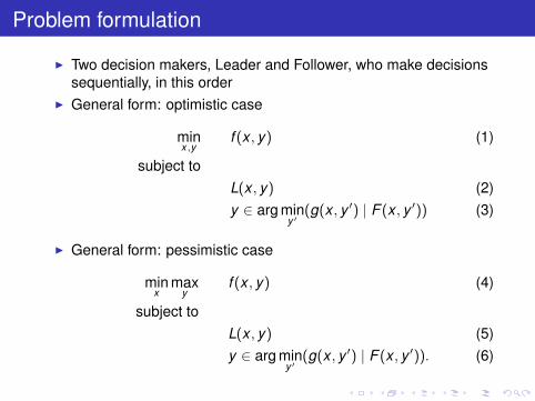
Problem formulation

I Two decision makers, Leader and Follower, who make decisionssequentially, in this order

I General form: optimistic case

minx,y

f (x , y) (1)

subject toL(x , y) (2)y ∈ arg min

y ′(g(x , y ′) | F (x , y ′)) (3)

I General form: pessimistic case

minx

maxy

f (x , y) (4)

subject toL(x , y) (5)y ∈ arg min

y ′(g(x , y ′) | F (x , y ′)). (6)

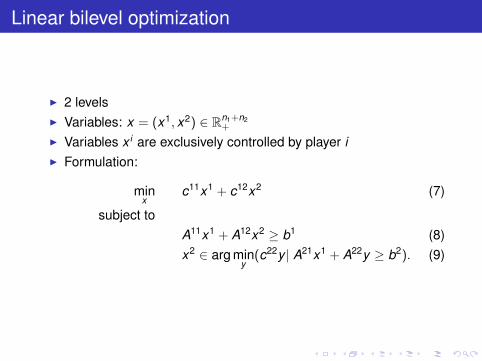
Linear bilevel optimization

I 2 levelsI Variables: x = (x1, x2) ∈ Rn1+n2

+

I Variables x i are exclusively controlled by player iI Formulation:

minx

c11x1 + c12x2 (7)

subject toA11x1 + A12x2 ≥ b1 (8)x2 ∈ arg min

y(c22y | A21x1 + A22y ≥ b2). (9)

The polynomial hierarchy

Definition (Polynomial hierarchy by Karp)Let L ⊂ S+ be a language over a finite alphabet. For any k ≥ 1,

I L ∈∑p

k if and only if ∃p1, . . . ,pk polynomials and L′ ∈ P suchthat for any x ∈ S+

x ∈ L iff (∃y1)p1 (∀y2)p2 . . . (Qyk )pk [(x , y1, . . . , yk ) ∈ L′]I L ∈ Πp

k if and only if ∃p1, . . . ,pk polynomials and L′ ∈ P such thatfor any x ∈ S+:x ∈ L iff (∀y1)p1 (∃y2)p2 . . . (Qyk )pk [(x , y1, . . . , yk ) ∈ L′]

Definition (Polynomial hierarchy by Stockmeyer)∑pk = NP(

∑pk−1) with

∑p0 = P

Πpk = co −NP(

∑pk−1)

Theorem (Wrathal)The two definitions are equivalent.

Complexity of multi-level programming

Theorem (Jeroslow)Bilevel linear programming is NP-hard.

Theorem (Jeroslow)(k + 1)-level linear programming is Σp

k -hard.

Theorem (Jeroslow)k-level integer (binary) programming is Σp

k -hard.

CorollaryUnless the polynomial hierarchy collapses at level 1, integer (binary)k-level programs cannot be modeled by mixed integer programs ofsize polynomial in the size of the input, for any k ≥ 2.

CorollaryUnless the polynomial hierarchy collapses at level 1, linear k-levelprograms cannot be modeled by mixed integer programs of sizepolynomial in the size of the input, for any k ≥ 3.

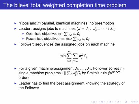
The bilevel total weighted completion time problem

I n jobs and m parallel, identical machines, no preemptionI Leader: assigns jobs to machines (J = J1 ∪ J2 ∪ · · · ∪ Jm)

I Optimistic objective: min∑

j∈J w1j Cj

I Pessimistic objective: min max∑

j∈J w1j Cj

I Follower: sequences the assigned jobs on each machine

minm∑

i=1

∑j∈Ji

w2j Cj

I For a given machine assignment J1, . . . , Jm, Follower solves msingle machine problems 1||

∑j w2

j Cj by Smith’s rule (WSPTorder)

I Leader has to find the best assignment knowing the strategy ofthe Follower

Results on bilevel total weighted completion timeproblem

Restriction Complexityno restriction decision version is NP-completew1 ≡ 1, w2 induces equivalent to P||

∑j Cj

an increasing proc. time orderw1 ≡ 1, w2 induces reduces to a specialA decreasing proc. time order MAX m-CUT problemw1 ≡ 1, w2 arbitrary FPTAS of Sahni for Pm||

∑j wjCj

m constant can be generalized

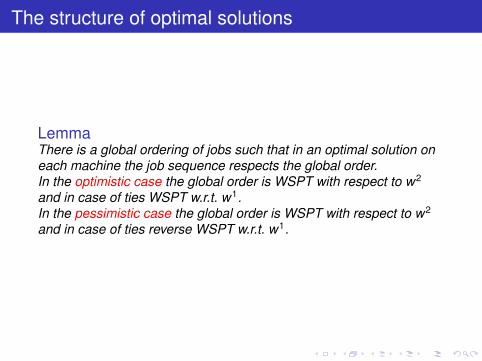
The structure of optimal solutions

LemmaThere is a global ordering of jobs such that in an optimal solution oneach machine the job sequence respects the global order.In the optimistic case the global order is WSPT with respect to w2

and in case of ties WSPT w.r.t. w1.In the pessimistic case the global order is WSPT with respect to w2

and in case of ties reverse WSPT w.r.t. w1.

Reduction to the MAX m-CUT problem

MAX m-CUT (optimization version)input: the number of vertices (of a complete graph) n, edge weightsce for all the n(n−1)/2 edges, a number m with m ≤ n (all data in Z+)output: a partitioning of the vertices into m disjoint classesV1, . . . ,Vm such that the total weight of edges between the classes ismaximized, i.e.,

max(V1,...,Vm)

m−1∑k=1

m∑`=k+1

∑i∈Vk ,j∈V`

cij

where the maximum is over all m-partitions of the n nodesReduction: the nodes are identified with the n tasks, and

cjk = pjw1k if

w2j

pj>

w2k

pk; or

w2j

pj=

w2k

pkand

w1j

pj≥

w1k

pk

A special MAX m-CUT problem

Special weights

If w1 ≡ 1 and w2j

pj>

w2k

pkiff pj > pk , then cjk = max{pj ,pk}

TheoremThere exists an optimal solution to MAX m-CUT such thatV1 = {1, . . . , k1},V2 = {k1 + 1, . . . , k2}, . . . ,Vm = {km−1 + 1, . . . ,m},where pj ≥ pk for j < k.

! " # $

% & '

(

! " % &

(

! " # $% & '# $ '

# $ '# $ '

CorollaryThe MAX m-CUT problem with the above weights can be solved bydynamic programming in polynomial time

The bilevel order acceptance problem

I There are n jobs with processing times pj , due-dates dj , andjob-weights w1

j ,w2j ; and a single machine

I Leader: selects a subset of jobs A (accepted jobs) to maximize∑j∈A w1

jI Follower: sequences the jobs non-preemptively to minimize∑

j∈A w2j Cj

I The solution is feasible iff the optimal solution chosen by theFollower meets the due-dates of all jobs in A

I If the Leader is optimistic, it selects A such that at least oneoptimal solution of the Follower meets all the due-dates

I If the Leader is pessimistic, it selects A such that all the optimalsolutions of the Follower with respect to A meets all thedue-dates

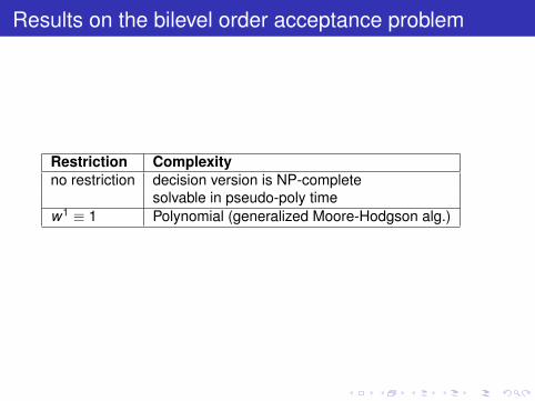
Results on the bilevel order acceptance problem

Restriction Complexityno restriction decision version is NP-complete

solvable in pseudo-poly timew1 ≡ 1 Polynomial (generalized Moore-Hodgson alg.)

A polynomial algorithm for the w1 ≡ 1 case

The Moore-Hodgson algorithm for 1||∑

Uj

1. Order the jobs in EDD order: d1 ≤ . . . ≤ dn

2. Starting with the first job, process the jobs one-by-one. If all jobscan be completed on time, stop. Otherwise, let k1 be the first jobsuch that

∑k1j=1 pj > dk1 . Remove from the first k1 jobs the one

with largest pj value, and proceed with the next job.

Modification for the bilevel order acceptance problem:

1. Order the jobs in the Follower’s WSPT order: j < k iff w2j

pj>

w2k

pk

and in case of ties if dj < dk (dj > dk )

Uncapacitated lot-sizing with backlogging (ULSB)

min

{n∑

t=1

(ptxt + ftyt + htst + gt rt ) | (11)− (15)

}(10)

where

xt + (st−1 − rt−1) = dt + (st − rt ), t = 1, . . . ,n (11)xt ≤ Myt , t = 1, . . . ,n (12)s0 = sn = r0 = rn = 0, (13)xt , st , rt ,≥ 0, t = 1, . . . ,n (14)yt ∈ {0,1}, t = 1, . . . ,n (15)

whereI The pt , ft , ht , gt are the cost parameters, the dt are the demandsI The xt , yt , st , rt are the variables

Some related work

I W. I. Zangwill, A backlogging model and a multi-echelon modelof a dynamic economic lot size production system – A networkapproach. Management Science, 15(9):506–527, 1969.

I A. Federgruen, M. Tzur, The dynamic lot-sizing model withbacklogging: A simple O(n log n) algorithm and minimal forecasthorizon procedure. Naval Res. Logitics 40, 459–478, 1993.

I Y. Pochet and L. A. Wolsey. Lot-size models with backlogging:Strong reformulations and cutting planes. MathematicalProgramming, 40:317–335, 1988.

I S. Kucukyavuz and Y. Pochet. Uncapacitated lot-sizing withbacklogging: the convex hull. Mathematical Programming, Ser.A, 118:151–175, 2009.

Network representation of ULSB

0

1 2 3 4 5

*

s1 s2 s3 s4r1 r2 r3 r4

x1x2 x3 x4 x5

d1d2 d3 d4 d5

x5

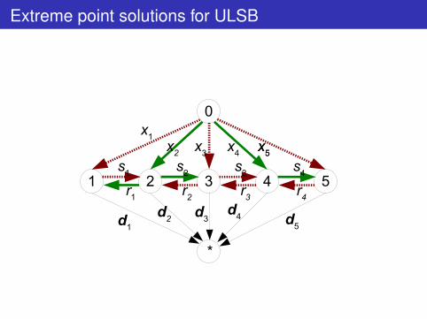
Extreme point solutions for ULSB

0

1 2 3 4 5

*

s1 s2 s3 s4r1 r2 r3 r4

x1x2 x3 x4 x5

d1d2 d3 d4 d5

x5

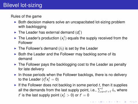
Bilevel lot-sizing

Rules of the gameI Both decision makers solve an uncapacitated lot-sizing problem

with backloggingI The Leader has external demand (d1

t )I The Leader’s production (x1

t ) equals the supply received from theFollower

I The Follower’s demand (δt ) is set by the LeaderI Both the Leader and the Follower may backlog some of its

demandI The Follower pays the backlogging cost to the Leader as penalty

for late deliveryI In those periods when the Follower backlogs, there is no delivery

to the Leader (r2t x1

t = 0)I If the Follower does not backlog in some period t , then it supplies

all the demands from the last supply point, i.e.,∑t

u=t′+1 δt , wheret ′ is the last supply point (x1

t′ > 0) or t ′ = 0

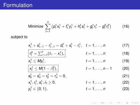
Formulation

Minimizen∑

t=1

(p1

t x1t + f 1

t y1t + h1

t s1t + g1

t r1t − g2

t r2t)

(16)

subject to

x1t + s1

t−1 − r1t−1 = d1

t + s1t − r1

t , t = 1, . . . ,n (17)

r2t =

∑tτ=1(δτ − x1

τ ), t = 1, . . . ,n (18)

x1t ≤ My1

t , t = 1, . . . ,n (19)

x1t ≤ M(1− β2

t ), t = 1, . . . ,n − 1 (20)

s10 = s1

n = r10 = r1

n = 0, (21)

x1t , r

1t , s

1t , δt ≥ 0, t = 1, . . . ,n (22)

y1t ∈ {0,1}, t = 1, . . . ,n (23)

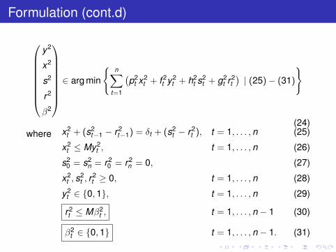
Formulation (cont.d)

y2

x2

s2

r2

β2

∈ arg min

{n∑

t=1

(p2

t x2t + f 2

t y2t + h2

t s2t + g2

t r2t)| (25)− (31)

}

(24)where x2

t + (s2t−1 − r2

t−1) = δt + (s2t − r2

t ), t = 1, . . . ,n (25)

x2t ≤ My2

t , t = 1, . . . ,n (26)

s20 = s2

n = r20 = r2

n = 0, (27)

x2t , s

2t , r

2t ≥ 0, t = 1, . . . ,n (28)

y2t ∈ {0,1}, t = 1, . . . ,n (29)

r2t ≤ Mβ2

t , t = 1, . . . ,n − 1 (30)

β2t ∈ {0,1} t = 1, . . . ,n − 1. (31)

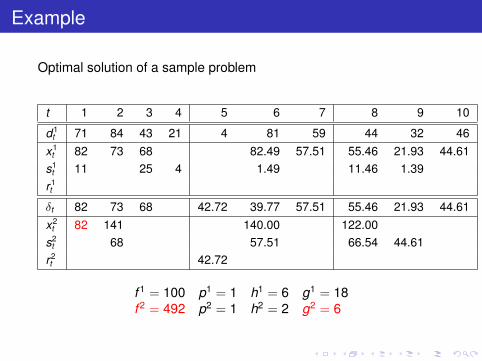
Example

Optimal solution of a sample problem

t 1 2 3 4 5 6 7 8 9 10

d1t 71 84 43 21 4 81 59 44 32 46

x1t 82 73 68 82.49 57.51 55.46 21.93 44.61

s1t 11 25 4 1.49 11.46 1.39

r 1t

δt 82 73 68 42.72 39.77 57.51 55.46 21.93 44.61x2

t 82 141 140.00 122.00s2

t 68 57.51 66.54 44.61r 2t 42.72

f 1 = 100 p1 = 1 h1 = 6 g1 = 18f 2 = 492 p2 = 1 h2 = 2 g2 = 6

Example

Optimal solution of a sample problem

t 1 2 3 4 5 6 7 8 9 10

d1t 71 84 43 21 4 81 59 44 32 46

x1t 82 73 68 82.49 57.51 55.46 21.93 44.61

s1t 11 25 4 1.49 11.46 1.39

r 1t

δt 82 73 68 42.72 39.77 57.51 55.46 21.93 44.61x2

t 82 141 140.00 122.00s2

t 68 57.51 66.54 44.61r 2t 42.72

f 1 = 100 p1 = 1 h1 = 6 g1 = 18f 2 = 492 p2 = 1 h2 = 2 g2 = 6

Formulation MIP-1

DefinitionLet OP2 be the set of those (x2, y2, s2, r2, δ) vectors such that∑n

t=1 δt =∑n

t=1 d1t , and (x2, y2, s2, r2) is an optimal solution for the

ULSB of the Follower w.r.t. demand δ.Let Z ULSB(δ) denote the optimum value of ULSB for fixed δ > 0

QuestionDoes OP2 admit a compact (extended) mixed integer formulation?

AnswerYES! Idea: use an extended formulation for ULSB with δ in theobjective function only.

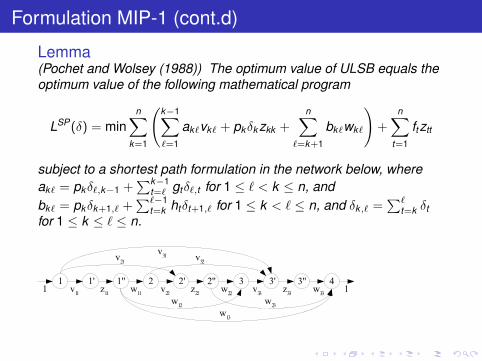
Formulation MIP-1 (cont.d)

Lemma(Pochet and Wolsey (1988)) The optimum value of ULSB equals theoptimum value of the following mathematical program

LSP(δ) = minn∑

k=1

(k−1∑`=1

ak`vk` + pkδk zkk +n∑

`=k+1

bk`wk`

)+

n∑t=1

ftztt

subject to a shortest path formulation in the network below, whereak` = pkδ`,k−1 +

∑k−1t=` gtδ`,t for 1 ≤ ` < k ≤ n, and

bk` = pkδk+1,` +∑`−1

t=k htδt+1,` for 1 ≤ k < ` ≤ n, and δk,` =∑`

t=k δtfor 1 ≤ k ≤ ` ≤ n.

1 1' 1'' 2 2' 2'' 3 3' 3'' 4v11 z11 w11 v22 z22 w22 v33 z33 w331 1

v21v31 v32

w12 w23w13

Formulation MIP-1 (cont.d)The dual of the shortest path formulation is

DSP(δ) = maxφ21 (32)

subject to

φ2t − φ2

k ′ ≤ ak,t , k = t , . . . ,nφ2

t′ − φ2t′′ ≤ p2

t δt + f 2t ,

φ2t′′ − φ2

k+1 ≤ bt,k , k = t , . . . ,n

for all t = 1, . . . ,n. (33)

By the strong duality of linear programming Z ULSB(δ) = DSP(δ) forany fixed δ ≥ 0.

Lemma(x2, y2, s2, r2, δ) ∈ OP2 if and only if

∑nt=1 δt =

∑nt=1 d1

t , and thereexists φ2 such that (x2, y2, s2, r2, β, δ, φ2) satisfies the constraints(25)-(31), (33), and the equation

n∑t=1

(p2

t x2t + f 2

t y2t + h2

t s2t + g2

t r2t)

= φ21. (34)


The complete formulation:

MIP-1 : min

n∑

t=1

(p1

t x1t + f 1

t y1t + h1

t s1t + g1

t r1t − g2

t r2t) (17)-(19),

(21)-(23),(25)-(31),(33),(34)

.

LemmaWe have the following correspondence between the feasible solutionsof the bilevel lot-sizing problem and that of MIP-1:

(i) Any feasible solution of MIP-1 can be projected onto a feasiblesolution of the bilevel lot-sizing problem of the same value.

(ii) Conversely, any feasible solution of the bilevel lot-sizing problemcan be extended to a feasible solution of MIP-1 of the samevalue.

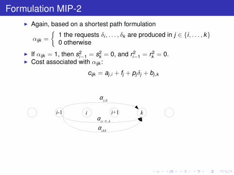
Formulation MIP-2I Again, based on a shortest path formulation

αijk =

{1 the requests δi , . . . , δk are produced in j ∈ {i , . . . , k}0 otherwise

I If αijk = 1, then s2i−1 = s2

k = 0, and r2i−1 = r2

k = 0.I Cost associated with αijk :

cijk = aj,i + fj + pjδj + bj,k

i-1 i+1αi, i +1 , k

k

αi, i, k

αi, k, k

i


MIP-2 : minn∑

t=1

(p1

t x1t + f 1

t y1t + h1

t s1t + g1

t r1t − g2

t r2t)

subject to the constraints of the Leader, and

r2t ≤ M(1− β2

t ), t = 1, . . . ,n − 1

β2t =

∑i≤t<j≤k

αi,j,k , t = 1, . . . ,n − 1

∑i≤t≤k

∑i≤j≤k

αi,j,k = 1, t = 1, . . . ,n

aj,i + fj + pjδj + bj,k + φi−1 ≥ φk , 1 ≤ i ≤ j ≤ k ≤ naj,i + fj + pjδj + bj,k + φi−1 ≤ φk −M ′(1− αi,j,k ), 1 ≤ i ≤ j ≤ k ≤ nφ0 = 0,αi,j,k ∈ {0,1}, 1 ≤ i ≤ j ≤ k ≤ n.

Extreme Point Solutions

DefinitionA solution to the bilevel lot-sizing problem is an extreme point solutionif the Follower’s part is an extreme point solution of ULSB withdemands δt .Assumption g2

t + h2t > 0 for all t = 1, . . . ,n − 1.

This assumption excludes that a solution with r2t s2

t > 0 is optimal forthe Follower.

LemmaUnder the assumption, if the bilevel optimization problem admits anoptimal solution, then it admits an extreme point optimal solution.

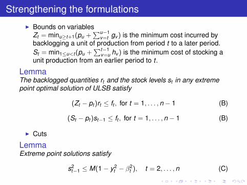
Strengthening the formulations

I Bounds on variablesZt = minu≥t+1(pu +

∑u−1v=t gv ) is the minimum cost incurred by

backlogging a unit of production from period t to a later period.St = min1≤u<t (pu +

∑t−1v=u hv ) is the minimum cost of stocking a

unit production from an earlier period to t .

LemmaThe backlogged quantities rt and the stock levels st in any extremepoint optimal solution of ULSB satisfy

(Zt − pt )rt ≤ ft , for t = 1, . . . ,n − 1 (B)

(St − pt )st−1 ≤ ft , for t = 1, . . . ,n − 1 (B)

I Cuts

LemmaExtreme point solutions satisfy

s2t−1 ≤ M(1− y2

t − β2t ), t = 2, . . . ,n (C)

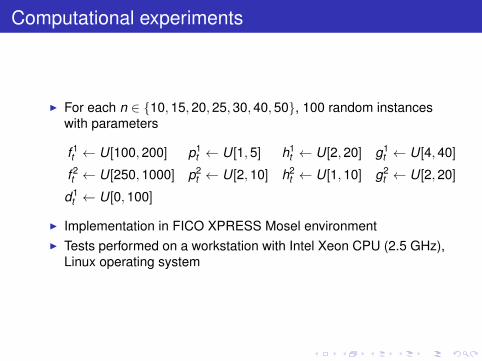
Computational experiments

I For each n ∈ {10,15,20,25,30,40,50}, 100 random instanceswith parameters

f 1t ← U[100,200] p1

t ← U[1,5] h1t ← U[2,20] g1

t ← U[4,40]

f 2t ← U[250,1000] p2

t ← U[2,10] h2t ← U[1,10] g2

t ← U[2,20]

d1t ← U[0,100]

I Implementation in FICO XPRESS Mosel environmentI Tests performed on a workstation with Intel Xeon CPU (2.5 GHz),

Linux operating system

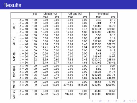
Resultsopt LB gap (%) UB gap (%) time (sec)

max avg max avg max avgM

IP-1

n = 10 100 0.00 0.00 0.00 0.00 0.49 0.16n = 20 100 0.00 0.00 0.00 0.00 9.91 1.14n = 30 100 0.00 0.00 0.00 0.00 188.00 16.75n = 40 88 17.36 0.89 16.99 0.47 1200.44 329.86n = 50 53 15.09 2.91 12.38 1.88 1200.90 749.97

MIP

-1B

n = 10 100 0.00 0.00 0.00 0.00 0.53 0.16n = 20 100 0.00 0.00 0.00 0.00 13.83 1.19n = 30 100 0.00 0.00 0.00 0.00 357.02 22.00n = 40 90 19.68 0.79 16.99 0.46 1200.30 322.78n = 50 59 14.41 2.51 11.85 1.94 1200.58 714.31

MIP

-1C

n = 10 100 0.00 0.00 0.00 0.00 0.61 0.18n = 20 100 0.00 0.00 0.00 0.00 8.41 1.20n = 30 100 0.00 0.00 0.00 0.00 248.62 16.07n = 40 92 16.99 0.60 17.82 0.46 1200.30 248.81n = 50 51 15.19 2.77 11.81 1.88 1200.65 730.48

MIP

-1C

B n = 10 100 0.00 0.00 0.00 0.00 0.76 0.27n = 20 100 0.00 0.00 0.00 0.00 8.82 1.54n = 30 100 0.00 0.00 0.00 0.00 158.35 14.74n = 40 96 17.02 0.46 16.99 0.44 1200.26 227.71n = 50 65 12.11 1.97 11.51 1.83 1200.55 645.94

MIP

-2 n = 10 100 0.00 0.00 0.00 0.00 35.65 17.93n = 20 0 70.73 43.06 2974.59 1515.28 1200.00 1200.00

MIP

-2B n = 10 100 0.00 0.00 0.00 0.00 46.83 10.57

n = 20 0 59.32 17.79 192.80 108.28 1200.00 1200.00

Documents

Diszkrét kétszintu optimalizálás