Discussion PaPer series

IZA DP No. 10592

Young-Il KimJungmin Lee

Does Single Motherhood Hurt Infant Health among Young Mothers?

februAry 2017

Any opinions expressed in this paper are those of the author(s) and not those of IZA. Research published in this series may include views on policy, but IZA takes no institutional policy positions. The IZA research network is committed to the IZA Guiding Principles of Research Integrity.The IZA Institute of Labor Economics is an independent economic research institute that conducts research in labor economics and offers evidence-based policy advice on labor market issues. Supported by the Deutsche Post Foundation, IZA runs the world’s largest network of economists, whose research aims to provide answers to the global labor market challenges of our time. Our key objective is to build bridges between academic research, policymakers and society.IZA Discussion Papers often represent preliminary work and are circulated to encourage discussion. Citation of such a paper should account for its provisional character. A revised version may be available directly from the author.

Schaumburg-Lippe-Straße 5–953113 Bonn, Germany

Phone: +49-228-3894-0Email: publications@iza.org www.iza.org

IZA – Institute of Labor Economics

Discussion PaPer series

IZA DP No. 10592

Does Single Motherhood Hurt Infant Health among Young Mothers?

februAry 2017

Young-Il KimSogang University

Jungmin LeeSeoul National University and IZA

AbstrAct

IZA DP No. 10592 februAry 2017

Does Single Motherhood Hurt Infant Health among Young Mothers?

Does single motherhood adversely affect infant health? This question is not easy to answer

because of the endogeneity of coresidence during pregnancy. In this paper, we exploit

quasi-natural variation in single motherhood from the moment of conception to that of

birth arising from marriageable age restrictions and the reform of the laws in Korea. The

Korean birth certificate dataset is unique in that it allows us to distinguish coresidence

and legal marital status and further to identify the duration of pregnancy period without

a partner. Results show that although coresidence with the partner during pregnancy is

seemingly beneficial for infant health, it is mostly driven by selection into coresidence.

Further, we do not find any significant advantage of legal marriage among young mothers.

JEL Classification: I12, J12, K36

Keywords: single motherhood, coresidence, marriage, marriageable age, birth weight, LBW, preterm birth, quasi-natural experiment

Corresponding author:Jungmin LeeDepartment of EconomicsSeoul National UniversitySeoul 08826South Korea

Email: jmlee90@snu.ac.kr

1 Introduction

The traditional family, which is typically comprised of a married couple and their biological chil-

dren, is vanishing in many parts of the world, as replaced by cohabitation and single parenthood

(Lundberg and Pollak, 2007; Stevenson and Wolfers, 2007). More children are born under non-

traditional types of households. This trend is challenging one of the basic premises of the economics

of the family. The rational choice theory of the family a la Becker (1991) postulates that “the main

purpose of marriage and families is the production and rearing of own children” (p. 135). How non-

traditional household structures affect children’s welfare should be an important question for policy

makers since household type defines crucial conditionality for many welfare and social programs.

Household production of child quality should essentially differ across alternative household

types. In particular, single parenthood is likely to be inferior to dual parenthood because households

of single parenthood cannot take such advantages as economies of scale, risk sharing, division of

labor, and specialization. However, it is difficult to identify the causal effect of single parenthood

on child quality because the lack of a parent should not be orthogonal to household production

for child quality; single- and dual-parent households are likely to differ in terms of unobservables

as well as observables, which are relevant for household production of child quality (Buckles and

Price, 2013; Finlay and Neumark, 2010). Identifying the causal effect of single parenthood on child

quality is also theoretically challenging because dual parenthood should be endogenized in a model

of intra-household resource allocation (Iyigun and Walsh, 2007).

In this paper, we examine whether single motherhood during pregnancy matters for infant

health at birth. We define single motherhood as the lack of the father in the household at any

time from conception to birth, regardless of legal marital status.1 Addressing the endogeneity of

the couple’s decision to live together, we exploit arguably exogenous variation in coresidence status

arising from marriageable age laws and the reform of these laws. The idea of using marriageable

age laws as the instrumental variables (IV) for coresidence is theoretically valid. A key determinant

of coresidence decision should be legal marriageability because 1) coresidence typically occurs on

the expectation of marriage and 2) coresidence with minors who are not legally eligible to marry is

less socially acceptable and therefore more costly.

In South Korea, the minimum marriageable age with parental consent was revised from 16 to

1We use the term ‘coresidence’ to indicate those couples who live together regardless of marital status. We avoidusing the term ‘cohabitation’ because the term commonly indicates in the literature only non-married couples wholive together.

1

18 in 2008, while the minimum marriageable age without parental consent remained at age 20

during the sample period. The marriage laws provide us with two sources of exogenous variation in

the probability of coresidence. First, the legislated change in the minimum age for marriage with

parental consent gives us an opportunity to use exogenous variation in the likelihood of coresidence

in the difference-in-differences context.2 Second, there is a discrete change in the coresidence rate

at age 20, which is too large to be explained by other things than the marriageable restriction at

that age. This provides us with another source of variation in coresidence, while the validity of

using this variation depends on whether it is possible to distinguish the effect of the age cutoff from

the age effect per se. We try to partial out the age effect by the parametric assumption that the

age profile of coresidence is quadratic. We show that our main conclusions are robust regardless of

whether we utilize this additional source of variation or not.

While households produce a variety of commodities in the Beckerian sense, we choose infant

health at birth as a measure of an output from household production since it is advantageous for the

purpose of our paper mainly in the two regards as follows. First, our main measure of infant health

is birth weight, which is measured at the exact moment of birth.3 Birth weight is therefore a highly

accurate measure of household production output because it entirely depends upon parental input

and endowments, as opposed to later outcomes that would also depend on children’s own attributes

and responses to parental investments. It seems that, for the same reason, earlier studies have used

birth outcomes as the output measures of household production, but they did not consider single

parenthood as a key input (Grossman and Joyce, 1990).

Second, recent studies in economics have found birth weight to be a strong predictor of children’s

later-life socioeconomic outcomes (Behrman and Rosenzweig, 2004; Almond et al., 2005; Black et

al., 2007). In particular, Figlio et al. (2014) found that the birth weight premium that we observe

in terms of later-life outcomes can be attributed by and large to the associated cognitive ability

gap. This means that if single motherhood during pregnancy reduces birth weight, the effect should

persist over the long run and thus the penalty of lower birth weight is hard to overcome.

Besides utilizing a novel source of exogenous variation in single motherhood, our paper makes

two additional contributions to the literature. First, we estimate the impact of the presence (or

lack) of a partner over the time period of pregnancy on infant health at birth.4 Many previous

2Dahl (2010) also uses different state laws on marriageability, working age, and compulsory education as IVs to findthat women who marry early are more likely to live in poverty and that women who drop out of school are morelikely to be poor later in their lives.

3We also look at two other birth weight related outcomes, such as low birth weight (LBW) and preterm birth.4Throughout the paper, we use the term ‘partner’ to indicate the father who lives together with the mother, whether

2

studies have considered only legal marital status at the time of birth, so could not have identify

whether the partner was present although they were not married.5 This data limitation may bias

the estimate for the effect of single parenthood, especially given the current trend of the decreasing

proportion of children born under legal marriage.6 The Korean administrative birth records allow

us to distinguish legal marital status and coresidence, separately. Reporting a child’s birth, parents

are required to report not only their legal marital status but also coresidence status.

Second, the Korean birth records provide us with the information on the start date of coresi-

dence. Combined with the information on the birth date, this allows us to establish when coresi-

dence began in reference to the time of conception.7 Therefore, we can estimate not only the effect

of single motherhood but also the effect of its duration during pregnancy. If the partner (father) is

a relevant input for the production of infant health, the length of pregnancy with or without the

partner should be more informative than the coresidence status at the time of birth.

There is a large body of literature on the effect of single motherhood on children, focusing on

their later-life outcomes such as educational attainment, labor market outcomes, and adulthood

well-being (Ribar, 2004). The results seem to be mixed. While it is quite obvious that single moth-

erhood is not beneficial for most children (Raatikainen et al., 2005), the penalty is not unambiguous

formarginal children—children of parents who are at the margin of marriage or coresidence. Indeed,

some studies found a negative effect for children residing with single mothers even after controlling

for family fixed effects (Ermisch and Francesconi, 2001; Gennetian, 2005), whereas other studies did

not (Bjorklund and Sundstrom, 2006). Using exogenous variation in the divorce rate arising from

unilateral divorce laws of the United States, Gruber (2004) found that children who lived in states

where divorce has been made easier by unilateral divorce laws grew up to be less educated and

to earn lower incomes. Page and Stevens (2004) followed up families with divorced parents in the

PSID and found that these families had substantially lower incomes and consumption, which imply

serious disadvantages for the children. However, Finlay and Neumark (2010) used state-by-year

variation in male incarceration rates as the IV for marital status and found no impact of divorce

on children’s later-life economic outcomes.

they are either legally married or merely cohabiting.5Grossman and Joyce (1990) controlled for the indicator that the mother is not married at the time of birth. Inter-estingly, they called the variable as “illegitimacy.” It is actually quite rare in the economics literature to distinguishbetween marriage and cohabitation. Kalenkoski et al. (2005) distinguished between cohabitation and legal marriagein their examination of parental child-care activities by family type. They found little difference between coresidingand married parents, using time-use survey data from the United Kingdom.

6For mothers who are younger than the legal marrying age, marriage is not possible, but coresidence is possible.7Throughout the paper, we use the term ‘dual parents’ to indicate both the couples who are legally married or merelycoresiding, distinguished from the single mothers.

3

Buckles and Price (2013) examined the impact of single motherhood on birth weight, just as our

study does. To avoid omitted variable bias, they used matched sibling data and exploited variation

in marital status within a mother between childbirths, controlling for time-invariant unobservable

characteristics of the mother. Discussing the limitations of their study, they pointed out that their

dataset contains only information on legal marital status and lacks information on coresidence

status. Thus, they could examine only the effect of legal marital status. Our study proposes a new

identification strategy to estimate the causal effect and examines the impact of coresidence as well

as that of marriage.

To summarize our main findings, we found that the status of coresidence is significantly corre-

lated with infant health at birth. The coresidence with the father during pregnancy is positively

associated with birth weight and negatively correlated with poor birth outcomes, such as LBW

and preterm birth. However, after addressing endogenous selection into coresidence, we found that

the positive effects disappear mostly and become statistically insignificant. This suggests that the

observed advantage of coresidence for infant health is basically driven by positive selection into

coresidence. For comparison with the results in the existing literature, we also estimated the effect

of legal marriage and found a similar result as that for coresidence; there is a positive correlation

between legal marital status and infant health, but there is no causal impact of marriage.

The remainder of this paper is organized as follows. In Section 2, we present research background

by introducing the literature related to the subject of this paper. In Section 3, we introduce the

dataset and present the summary statistics of the variables that we use in our regression analysis.

Section 4 presents the empirical strategy and the estimation results. In Section 5, we examine

potential econometric problems and present robustness checks. Section 6 concludes this paper.

2 Research Background

2.1 Increasing Prevalence of Single Motherhood

The decrease in the proportion of children born under legal marriage is globally observed. In the

United States, out-of-wedlock births account for 44.3% of total births in 2013, a rapid increase

from below 30% in 1980, peaking at 51.8% in 2007 and 2008 (Martin et al., 2015). In Europe,

39% of births in European Union were out of wedlock in 2011, doubling over the past two decades

(Associated Press, 2010). In eight European countries, non-marital births accounts for more than

50% of all births while in Iceland it accounts for 67% of all births (PEW Research Center, 2014).

4

This phenomenon is more prevalent among young mothers. In the United States, children born

outside of marriage surpassed 50% of total births among mothers under 30 years of age (DeParle

and Tavernise, 2012). The largest single group in the United States for non-marital first births is

teenagers (Whitehead and Pearson, 2006). Approximately half of all non-marital births occurred

to teen mothers. Non-marital births for teen mothers increased from 15% in 1960 to 80% in the

21st century (Martin et al., 2006; Ventura and Bachrach, 2000), resulting from coresidence or

non-coresiding single births.

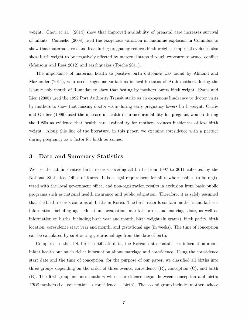
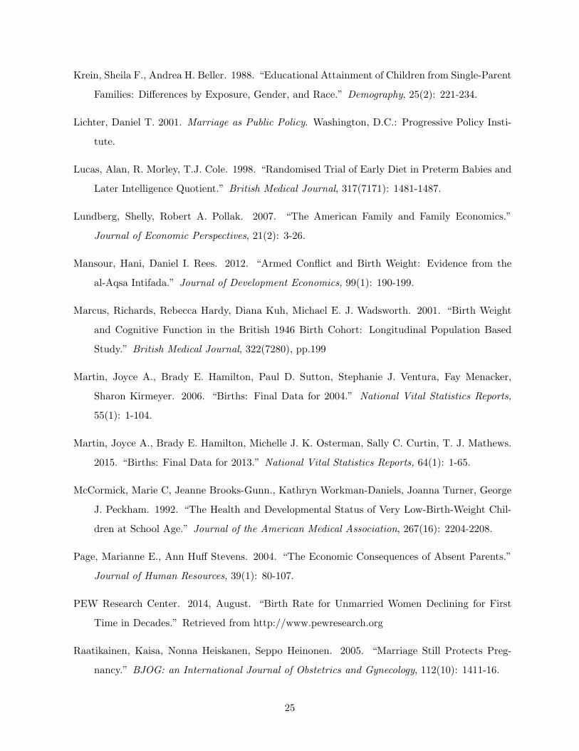
In our dataset from Korea, the ratio of mothers who are not coresiding when conception takes

place is increasing, and the trend is driven mainly by young mothers. Figure 1 shows that the

percentage of those mothers has increased from 17.4% in 1997 to 24.0% in 2011 for the mothers

who are 23 or older. For the same group, the percentage of mothers who never coreside by birth

has jumped from 0.3% to 1.2%. The increase is much greater for young mothers aged 16 to 22.

In this group, the percentage of births to mothers are not coresiding when conception takes place

increased from 25.3% to 47.8%. The percentage of mothers who never start coresiding by the time

of birth increased from 0.6% to 9.6% during the same period.

The increase in out-of-wedlock births among young mothers is a social concern. Out-of-wedlock

births have been found to have negative effects on children in the long run in many respects,

including education, and crime (Barber, 2006; Krein and Beller, 1988). Children born to unmarried

mothers may face initial health disadvantages, which profoundly impact their economic outcomes

later in life. Unfavorable birth outcomes directly incur substantial private and public costs. For

example, according to a report by the Institute of Medicine (2007), the health-care cost of preterm

birth amounts to $51,600 per infant. Furthermore, low birth weight and premature babies face

greater risks of infant mortality and disabilities. A growing body of evidence indicates that health

conditions at birth persistently influence later-life outcomes, such as adulthood health, education,

earnings, and well-being (Almond et al., 2005; Black et al., 2007; Currie et al., 2010; Heckman et

al., 2012).

Unmarried pregnancies may influence infant health in several channels. The absence of a part-

ner, who is an additional income earner as well as a source of emotional support, may have financial

and psychological influences on pregnant women who are neither married nor cohabitating and, by

extension, on their fetuses. Indeed, many studies in obstetrics and demography have reported that

out-of-wedlock pregnancy has a negative impact on infant health through these channels (Bennet,

5

1992; Bird et al., 2000).8

2.2 Economic Significance of Birth Outcomes and Determinants

Birth outcome is a topic of great interest to economists because its long-run effects on health, cog-

nitive development, and socioeconomic status are substantial. A growing number of studies have

found that health conditions at birth and during childhood have a significant long-term impact on

adulthood health, education, and labor-market outcomes. Numerous medical studies have shown

that fetal and infant health issues, especially low birth weight, have a persistent impact on various

adulthood diseases, including overall morbidity (McCormick et al., 1992), IQ (Lucas et al., 1998),

and cognitive disabilities (Marcus et al., 2001). Several studies in economics have shown the im-

pact of birth weight on economic variables that are closely related to human capital accumulation.

Using monozygotic twin data, Behrman and Rosenzweig (2004) found that higher birth weight

improves adult health and earnings. Black et al. (2007) also used within-twin variations to show

the significant long-term impact of birth weight on adult stature, IQ, earnings, and educational

attainment. The detrimental long-run impact of low birth weight may be even longer through an

intergenerational effect. Currie and Moretti (2007) found that there is significant intergenerational

transmission of low birth weight, and the impact is even stronger for low-income groups. Further-

more, many studies have found a strong long-run impact of childhood health, which is substantially

affected by birth outcome, on adult labor market and education outcomes.

The factors that affect birth outcomes are numerous and extensive. The WHO (2004) reported

biological factors (e.g., the baby’s sex, the mother’s age and weight, birth parity, and the presence

of disease in the mother), behavioral factors (e.g., nutritional intake during pregnancy and health-

related habits), and socioeconomic factors (e.g., education, income, and employment status) as

the main determinants for birth weight. Many studies have shown that the health status and

health-related behavior of the mother are significant determinants of birth outcomes.

Abrevaya and Dahl (2008), using maternally-matched data, found that smoking negatively

affects birth weight. Using prenatal exposure to the Super Bowl as a proxy for an increased

exposure to maternal alcohol and tobacco use, Duncan et al. (2012) found that exposure to the

Super Bowl lowered birth weight, and the emotional cues from upset wins further lowered birth

8In light of the evidence, a number of marriage-promotion policies have been enacted to improve child outcomes forsingle mothers. In the United States, for example, the 1996 welfare reforms and the Healthy Marriage Initiativeincluded in the 2006 TANF reauthorization aim to promote two-parent families and to prevent out-of-wedlockchildbearing (Finlay and Neumark, 2010). Additional pro-marriage policies at the state and local levels have focusedon poor urban women (Lichter, 2001).

6

weight. Chou et al. (2014) show that improved availability of prenatal care increases survival

of infants. Camacho (2008) used the exogenous variation in landmine explosion in Columbia to

show that maternal stress and fear during pregnancy reduces birth weight. Empirical evidence also

show birth weight to be negatively affected by maternal stress through exposure to armed conflict

(Mansour and Rees 2012) and earthquakes (Torche 2011).

The importance of maternal health to positive birth outcomes was found by Almond and

Mazumder (2011), who used exogenous variations in health status of Arab mothers during the

Islamic holy month of Ramadan to show that fasting by mothers lowers birth weight. Evans and

Lien (2005) used the 1992 Port Authority Transit strike as an exogenous hindrance to doctor visits

by mothers to show that missing doctor visits during early pregnancy lowers birth weight. Currie

and Gruber (1996) used the increase in health insurance availability for pregnant women during

the 1980s as evidence that health care availability for mothers reduces incidences of low birth

weight. Along this line of the literature, in this paper, we examine coresidence with a partner

during pregnancy as a factor for birth outcomes.

3 Data and Summary Statistics

We use the administrative birth records covering all births from 1997 to 2011 collected by the

National Statistical Office of Korea. It is a legal requirement for all newborn babies to be regis-

tered with the local government office, and non-registration results in exclusion from basic public

programs such as national health insurance and public education. Therefore, it is safely assumed

that the birth records contains all births in Korea. The birth records contain mother’s and father’s

information including age, education, occupation, marital status, and marriage date, as well as

information on births, including birth year and month, birth weight (in grams), birth parity, birth

location, coresidence start year and month, and gestational age (in weeks). The time of conception

can be calculated by subtracting gestational age from the date of birth.

Compared to the U.S. birth certificate data, the Korean data contain less information about

infant health but much richer information about marriage and coresidence. Using the coresidence

start date and the time of conception, for the purpose of our paper, we classified all births into

three groups depending on the order of three events; coresidence (R), conception (C), and birth

(B). The first group includes mothers whose coresidence began between conception and birth;

CRB mothers (i.e., conception → coresidence → birth). The second group includes mothers whose

7

coresidence did not start until birth; noR mothers (conception → birth with no coresidence). The

last group includes mothers whose coresidence started before conception; RCB mothers (coresidence

→ conception → birth).9

In our main analysis, we compare CRB mothers with noR mothers, which allows us to estimate

the impact of coresidence conditional on pregnancy.10 In our supplementary analysis, we compare

mothers by legal marital status at birth to estimate the effect of legal marriage, mainly for compar-

ison with previous literatures. Lastly, we compare RCB mothers with CRB and noR mothers and

determine whether coresidence prior to conception makes any difference in infant health at birth.11

Table 1 presents summary statistics for birth outcomes and mothers’ characteristics in corre-

lation with coresidence and marital status at birth. Out of a total of 7,790,728 births between

1997 and 2011, we exclude 3,907,887 second or higher parity births and 19,923 observations with

missing key variables. Then, we use 246,378 births from young mothers aged between 16 and 22,

around legislated marriageable age. Among them, 28% are CRB mothers and 3% are noR mothers.

On average, the CR ratio—the duration between conception (C) and coresidence (R) out of total

gestation weeks, formally defined in the next section in equation (3)— shows that CRB mothers

spend 36% of their pregnancy time without a partner. Legally married mothers still spend 12% of

their pregnancy time without a spouse because some of them get married after conception.

It is notable that all three birth outcomes (birth weight, LBW and premature birth) are more

favorable for CRB and RCB mothers than for noR mothers, and for married mothers than for

unmarried mothers. This seems to suggest that there is a positive impact of coresidence and

marriage on infant health. For CRB mothers, average birth weight is 130 grams higher than for

noR mothers. LBW and premature birth ratios are less than half of those for noR mothers. The

patterns are similar for married mothers, compared to unmarried mothers.

Table 1 also shows that mothers differ somewhat in observable characteristics based on coresi-

dence and marital status. CRB and RCB mothers have higher education levels than noR mothers

do, and married mothers have higher education levels than unmarried mothers do, on average.

Since most of the women in our sample are still school-aged, age strongly correlates with years

of schooling. RCB and CRB mothers are more likely than noR mothers to give birth at a hos-

pital, and married mothers are more likely than unmarried mothers to give birth at a hospital.

9Since gestational age is reported in weeks, the timing of conception is likely measured with errors, which can leadus to misclassify the mothers. This concern is addressed in Section 5.1.

10In Section 5.3, we will check potential biases due to selection into pregnancy.11We also compared married CRB and cohabiting CRB versus noR mothers. The results are quite similar to thosefrom our main analysis.

8

These differences in observable characteristics give rise to a concern about potential selection on

unobservables.

4 Estimation and Results

4.1 Empirical Strategy

Our main objective is to estimate the impact of coresidence on infant health by comparing CRB

mothers with noR mothers, who are different in their decision of coresidence after conception.

Selection into coresidence may as well be driven by unobservable traits, hence CRB and noR

mothers may differ in unobservable traits. We address the endogeneity problem of coresidence by

the IV method.

First-stage equation: We exploit exogenous variation in coresidence status by legal marriageabil-

ity defined by marriageable age legislation and the reform of the legislation. We use two dummy

variables as IVs, one indicating eligibility to marry without parental consent (NoConsent) and the

other eligibility to marry with parental consent (Consent). The first-stage equation is as follows:

CRBit = α1Consentit + α2NoConsentit + κ1Ageit + κ2Age2it +Xitγ1 + τ1t + ϵ1it (1)

where subscripts represent individual birth i at year t. CRBit is the indicator for CRB mothers,

which can be formally written as the following:

CRBit = 1[τCit < τRit ] (2)

where τCit is the time of conception and τRit is the start time of coresidence. The indicator indicates

that conception is ahead of coresidence. The control group consists of noR mothers.

Alternatively, as the dependent variable in equation (1), we use a continuous variable, which is

the proportion of pregnancy period without a partner:

CRRatioit = max{τBit − τRitτBit − τCit

, 1} (3)

where τBit is the time of birth. The denominator, (τBit − τCit ), is the length of gestation. Thus, this is

a measure of the intensity of coresidence treatment, the ratio of the duration of pregnancy between

conception (C) and coresidence (R) out of the whole gestation weeks (which we call as the CR

9

ratio). The variable is set to be 0 for noR mothers because they never coreside during pregnancy.

For robustness, we use both CRBit and CRRatioit but, for expositional simplicity, explain the

estimation models using the first.

The first two variables on the right-hand side in equation (1) are our IVs. Consentit is the

indicator of whether the mother must have parental consent to marry. Specifically, the variable

indicates whether she was between the ages of 16 and 19 until 2007 or between 18 and 19 since

2008 when the cutoff age for marriageability with parental consent was changed. NoConsentit is

the indicator of whether the mother can marry without parental consent (whether she is 20 years

of age or older). It is reasonable to assume that the pure age effect on coresidence is smooth

and continuous at around age 20 without any arbitrary restriction. It seems reasonable to specify

the age profile of coresidence given the relatively narrow range of age in our sample. Thus, after

controlling for age and age squared, α2 is likely to be the effect of the age cutoff. Since legal

marriageability should increase the probability of coresidence (because coresidence is more likely

among marriageable couples and future marriage is often a condition for coresidence), we expect

both α1 and α2 to be positive.

Note that our second IV is valid only if the quadratic specification can fully capture the pure

age effect of coresidence. Although this assumption is not unreasonable in our sample, we still

check the robustness of our results to this assumption in two ways. First, we only use the first

IV by restricting the sample to those under the age of 20 and see the robustness of our findings.

Second, we specify the age effect in a fully nonparametric way, that is, by controlling for all age

dummies, as in the following equation and, again, use the first instrument only. The nonparametric

specification actually allows us to test whether the age cutoff for marriageability without parental

consent indeed affects the likelihood of coresidence.

CRBit = α · Consentit +

22∑p=17

θpAgeip +Xitγ1 + τ1t+ ϵ1it (4)

where Ageip is the indicator variable for age p, which takes values between 17 and 22. We can

check the validity of our second IV by testing whether θ20 differs so much from θ19 that there is

a discrete jump in the coresidence rate, which is large enough for us to argue that it should be

caused by the cutoff age for marriageability. In this sense, this strategy somewhat resembles the

regression discontinuity approach.

In both equations (1) and (4), vector Xit includes control variables such as the mother’s demo-

10

graphic characteristics, which includes education level (two dummy variables, one for high school

graduation, and the other for college or more), the baby’s sex, multiple births (twins, triples, or

more), month of birth, and province of birth. Lastly, τ1t represents the birth year fixed effect, which

is expected to subsume any macro-level impact on infant health.

Second-stage equation: The second-stage equation is as follows:

Yit = β · CRBit + ρ1Ageit + ρ2Age2it +Xitγ + τt + ϵit (5)

where the dependent variable is one of the following birth outcomes: birth weight (in kilograms),

low birth weight (LBW, defined as birth weight under 2,500 grams), and preterm birth (defined as

the gestation weeks of less than 37 weeks). For LBW and preterm birth, we estimate the equation

using bivariate-probit since the dependent variables and the endogenous variable (CRBit) are both

dummy variables. When the endogenous variable is CRRatioit, which is continuous, we use IV-

probit to estimate the equation.12 The second-stage equation corresponding to the first-stage

estimation described in equation (2) is as follows:

Yit = β · CRBit +

22∑p=17

θpAgeip +Xitγ + τt + ϵit (6)

where all other variables are identically defined as in equation (5). As in equation (4), age is

included as a dummy variable. The second-stage estimation results for equation (5) are reported

in Tables 3–5, and the results for equation (6) are reported in Panel B of Table 7.

For comparison with previous studies that have examined the effect of legal marriage at birth

rather than coresidence, we also estimate the effect of marital status at time of birth by using the

same equation as (5), with the indicator for CRB mothers replaced with the indicator for married

mothers at the time of birth. Mothers who are not eligible for marriage without parental consent

(aged 16-17 after 2008) should not be legally married. However, we observe that out of 1,285 young

mothers, 221 mothers were reported to be married at the time of birth. Therefore, we take this

as an indication of greater commitment and stronger union for legally non-marriageable mothers.

The proportion of pregnancy period without a partner does not change with marital status; hence,

the analysis using the continuous explanatory variable should not be replicated.

Lastly, we examine if RCB mothers differ from CRB mothers and noR mothers:

12Even if we use linear probability models, the results are not different.

11

Yit = β1 · CRBit + β2 ·RCBit + ρ1Ageit + ρ2Age2it +Xitγ + τt + ϵit (7)

where RCBit is the indicator of RCB mothers. The control group is noR. This analysis compares the

birth outcomes of RCB and CRB mothers to those of noR mothers. β1 should capture any benefits

from post-conception coresidence, whereas β2 should capture any benefits from coresiding for the

full period of pregnancy. We also replace the indicator variables for RCB and CRB mothers with

the proportion of pregnancy period without a partner. The results for equation (7) are summarized

in Panel B of Table 6. In the table footnote, we report Angrist-Pischke multivariate F test statistics

to test the weakness of our instruments separately.

4.2 Empirical Results

4.2.1 First-Stage Results

In Table 2, we present the results of the first-stage equations (1) and (4). Columns (1) and (2) use

the indicator for CRB mothers as the dependent variable, and columns (3) and (4) use the CR ratio

as the dependent variable. Columns (1) and (3) present the results of equation (1), using both IVs

under the assumption that the age profile is quadratic. Columns (2) and (4) present the results of

equation (4), taking only the time-varying IV while controlling for all age dummies. The analysis

takes the age of 16 as the baseline age.

The results show that our IVs have significant and positive effects on both the CRB status and

the CR ratio. Specifically, in column (1), those mothers who are eligible to marry with parental

consent are by 28 percentage points more likely to start coresidence during pregnancy than those

who are not. Somewhat surprisingly, the effect of marriageability without parental consent is

similar in magnitude. Column (3) shows that marriageability with parental consent significantly

reduces the proportion of pregnancy period without a partner by 17 percentage points, which

is approximately 6.7 weeks, given that average gestation duration is 39.4 weeks. The effect of

marriageability without parental consent is again quite similar. The first-stage F statistic and

Hansen’s J test statistic support the relevance and validity of our IVs, as reported in the bottom

of Tables 3-5.

The results in columns (2) and (4) are similar to those in columns (1) and (3), respectively.

Mothers who are eligible to marry with parental consent were 30% more likely to initiate coresidence

during pregnancy. The CR ratio is 18 percentage point less than that of mothers who are not eligible

12

to marry. The results suggest that a substantial number of couples actually fail to receive parental

consent. This may be indicative of South Korean culture, where coresidence without legal marriage,

especially for teenage girls, largely brings disapproval.

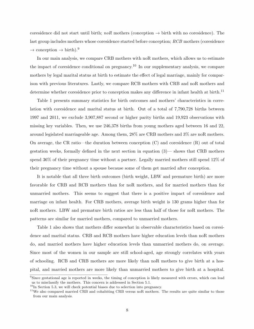
In Figure 2, we plot the estimates in Table 2 to visualize the effect of the cutoff age for legal

marriageability without parental consent. Panel A presents two age profiles, one based on the

estimates in column (1) of Table 2 (left) and the other based on the estimates in column (2) of

Table 2 (right). Both graphs are normalized by setting the effect at age 16 to be zero. When

marriageability with and without partner are both exclusively estimated, as in column (1), the age

profile clearly shows a discrete jump in the likelihood of coresidence at age 20. Panel A shows that

even when all ages are nonparametrically controlled as dummy variables and only marriageability

with parental consent is controlled, there is a discrete change in the coresidence rate at the cutoff

age. Similarly, using the estimates from column (3) of Table 2 (left) and column (4) of Table 2

(right), Panel B also shows that the change in the coresidence rate is visible at the cutoff age under

both specifications. This relieves the concern about our second IV.

4.2.2 Second-Stage Results

Results for birth weight: Table 3 shows the results from the second-stage equation using birth

weight as the dependent variable. In columns (1) and (2), we use the indicator variable for CRB

mothers and in columns (3) and (4) we take into account the treatment intensity using the CR

ratio. Columns (1) and (3) present OLS estimates, and columns (2) and (4) show IV estimates.

The OLS results in column (1) show that coresidence during pregnancy correlates with about 91

gram increase of birth weight. The results in column (3) show that one standard deviation decrease

in the CR ratio (0.26 from Table 1) is associated with an increase in birth weight of 19 grams (=

0.073*0.26).

However the IV results indicate little effect of coresidence on birth weight. In both columns (2)

and (4), the estimates are statistically insignificant. One might think that the standard errors of

IV estimates are inflated. However, the results show that the estimates are not only statistically

insignificant but also their magnitudes are close to zero and economically insignificant.

The results for other control variables are overall consistent with prior expectations. For ex-

ample, we find that boys are approximately 90 grams heavier than girls. Babies born to mothers

with either high-school education or college or higher education are approximately 30 grams heavier

than those born to mothers with less than high-school education. Unsurprisingly, birth weight for

13

multiple births is substantially lower than for single births (by approximately 870 grams). The

estimates for these variables are almost identical between OLS and IV estimations.

Results for LBW: Table 4 presents the results for LBW. Columns (1) and (3) present the sim-

ple probit results, and columns (2) and (4) present the bivariate-probit and IV-probit estimates,

respectively. In the table, we present marginal effects evaluated at sample means. The results in

column (1) show that coresidence is associated with a reduction in LBW by 2.6 percentage points.

In column (3), one standard deviation decrease in the CR ratio is correlated with a 0.6 percentage

point increase in the rate of LBW incidence. The effect is substantial, considering that the average

incidence of LBW is 7.1% for noR mothers.

However, as we found about birth weight, the benefit of coresidence mostly disappears after

the selection issue is addressed, as shown in columns (2) and (4). The IV estimates are not only

statistically insignificant but also very close to zero.

Some other results are worth noting. We find that boys are approximately 6% less likely to be

born with low birth weight, and higher-educated mothers are significantly less likely to have LBW

babies. Multiple births significantly increase the probability of LBW. These results are consistent

with the previous findings in the literature.

Results for preterm birth: Preterm birth, a birth with a gestational period of less than 37

weeks, is another key birth outcome with significant implications for infant health as well as long-

term economic outcomes. Table 5 presents the results, the marginal effects evaluated at sample

means. We find that coresidence is correlated with a reduction in the incidence of preterm birth

by 4 percentage points, and a one standard deviation decrease in the CR ratio is correlated with

an increase in the incidence of preterm birth by 1 percentage point, as illustrated in columns (1)

and (3). Unlike birth weight and LBW, coresidence seems to have a causal and positive effect on

preterm birth. In column (2), we find that coresidence reduces the probability of preterm birth

by 2.9 percentage points. However, notice that the effect is much smaller than the estimate in

column (1) and statistically only marginally significant. Also, when the CR ratio is used in column

(4), the coefficient becomes statistically insignificant and the magnitude of coefficient substantially

decreases. Therefore, we conclude that there is little causal effect of coresidence on the likelihood

of preterm birth.

Marriage premium: One might think that we failed to find any positive effect of coresidence

because coresidence is a less binding relationship than marriage. Thus, we examine the effect of

14

legal marriage by using the same specifications that we have used so far for coresidence. Also the

results about marriage are more comparable to the findings in the literature since previous studies

are focused on the effect of parents’ marital status on offsprings. In Table 6, we present only the

estimates of our main interest. Panel A presents the results of the analysis comparing married

and unmarried mothers. In columns (1), (3) and (5) where we do not resolve the endogeneity of

marriage, we find that birth weight for married mothers is on average 62 grams heavier, the LBW

probability is 1.8 percentage points lower, and the preterm birth probability is 2.7 percentage points

smaller than for unmarried mothers. However, similar to what we found about coresidence, we find

no causal effect of marriage on birth weight and LBW. On the other hand, consistent with the

results presented in column (2) of Table 5, we find that marriage reduces the probability of preterm

birth by 1.6 percentage point. But the estimate is only marginally significant and smaller than that

in column (5).

Coresidence prior to conception: So far we have excluded RCB mothers, those who started

coresidence before conception, from our analysis. One might be curious that the start of coresidence

before conception makes any difference. Panel B1 in Table 6 presents the results of the analysis

that compares CRB and RCB mothers, separately, with noR mothers. Again, the results without

addressing the endogeneity of coresidence show that both CRB and RCB mothers have more

favorable birth outcomes compared to noR mothers. However the IV estimates show that there is

actually no significant difference in terms of birth weight and LBW between RCB and noR mothers.

But we find that RCB mothers are 2 percentage point less likely to have preterm birth than noR

mothers. Lastly, for the sample including RCB mothers with the CR ratio set to be one, the results

in panel B2 show that all IV estimates for the CR ratio are statistically insignificant for all three

birth outcomes.

4.2.3 Possible Explanations

Our findings show that while coresidence and infant health at birth are positively correlated, there

is no causal relationship. This suggests that those young mothers who select into coresidence

should have unobservable characteristics that are favorable for infant health, but coresidence per

se has no exclusive additional benefit. One possible explanation for this result is related to the

degree of the contribution to be made by the partner for ameliorating infant health. For young

mothers like those in our sample, their partners are likely to have lower socioeconomic status,

15

so they are less capable of helping their pregnant partner. Even worse, they might have some

behavioral problems, such as drinking and smoking, that may have a negative effect on pregnant

women and their fetus. Then, they might be unable to provide enough support, either financial or

emotional, to make any meaningful contribution to infant health. This possibility was also pointed

out in Finlay and Neumark (2010). Using state-by-year variation in the male incarceration rate

as the IV for the marriage rate, they found that the impact of marriage on children’s educational

outcomes is actually negative for Hispanic mothers. To explain this puzzling finding, they suggested

the possibility that potential spouses available to those Hispanic mothers are likely to be of lower

socioeconomic status and the mothers might be better off without spouse.

Another possible interpretation for our findings is related to the quality of alternative maternal

care available to young mothers. For young pregnant mothers, a substitute to support from their

partner is informal and public assistance from parents, friends or the government. It is likely that

those mothers between the ages of 16 and 22 are living together with their parents, especially in

Korea where it is conventional for adult offsprings to live with their parents until the moment

of marriage. Therefore, if they opt not to coreside with their partner, they could receive some

compensatory support from their parents, which might be better than what they would receive

from their potential mate. Then, those whose parents are more willing and able to help their

pregnant young daughters would choose not to coreside with their partner. In this case, even

thought there is positive contribution to in-utero care made by the partner, but it may not be

greater than what those alternative caregivers or the different levels of governments can provide for

those young single mothers.

Lastly, it is worth noting that our finding of the lack of the marriage premium is in contrast

with the finding of Buckles and Price (2013). They found a sizable positive impact of marriage

on birth outcomes. Of course, it is difficult to explain different results in two studies for some

obvious reasons, such as differences in population of the study, data and estimation method. For

example, they excluded mothers under the age of 18 whereas we included those young mothers.

Also, they estimated the fixed-effect model to control for time-invariant maternal characteristics,

while we took the IV approach. Also, from the perspective of our explanation in this subsection,

the differences in the degree of social and family care for single mothers between Korea and the

United States might account for the differences in the results between two countries.

16

5 Supplementary Analysis

5.1 Robustness Checks

In this subsection, we conduct a few robustness checks. First, as a way of relieving the concern

about our second IV, we simply drop those aged 20 or above from the sample and use only the time-

varying IV. Panel A in Table 7 presents the results. We present the estimates of our main interest

(each estimate is from a separate regression). The results are similar to our main results that we

obtain using both IVs on the full sample. For example, the OLS estimate using the restricted

sample indicates an increase in birth weight by 91 grams. The corresponding estimate of the full

sample analysis was identical in Table 3, column (1). However, consistent with what we found

for the whole sample, the IV estimates across all specifications are not statistically significant and

much smaller in magnitude compared to the corresponding estimates without IV.

Next, to check the robustness of our results to the specification of the age effect, we report in

Panel B the results of equation (6) with age fixed effects. The results are also quite similar to our

previous results. The estimates without addressing the endogeneity of coresidence show significant

and positive correlations between coresidence and birth outcomes, while there is no causal effect

of coresidence according to the IV estimates. The IV estimate of preterm birth turns out to be,

albeit marginally, statistically significant but, just as in the previous results, the effect becomes

insignificant when we use the CR ratio. We believe that this reduces the concern regarding any

bias from misspecification of the age effect.

As mentioned earlier, gestation length is measured in weeks rather than in days, and this may

result in a bias due to measurement error. In addition, even when correctly measured, mothers in

their early stage of pregnancy may be unaware of their pregnancy, hence their decision to coreside

is independent of the fact of conception. To deal with this kind of problem, we drop these mothers

who started coresidence within two weeks of conception. Panel C presents the results using this

restricted sample. We find that the results are similar to our previous results.

Lastly, we attempt to define legal marriageability more conservatively. The concern is that the

administrative birth records provide the mother’s age only in years, so we cannot precisely define

legal marriageability at the time of conception. For example, let us consider those mothers who

were 20 years old at the time of childbirth. For these mothers, it is difficult to determine whether

they were eligible for marriage without parental consent at the time of conception. However, it is

certain that mothers who were 21 years of age at the time of childbirth must have been marriageable

17

without parental consent at the time of conception because the length of gestation should not be

longer than one year. Based on this idea, we re-define the cutoff age for marriage without consent

from 20 to 21 and that for marriage with consent from 16 to 17 before 2008 and from 18 to 19

afterwards.

Panel D presents the results using these alternative definitions. Overall, the IV results again

indicate that coresidence during pregnancy does not have any significant effect on birth outcomes,

except for preterm birth when the indicator for coresidence status is used. But it is not obvious

that coresidence actually decreases the likelihood of preterm birth, as we find no significant effect

when we use the CR ratio.

5.2 Resolution of Pregnancy

One limitation with birth record data is that we do not observe abortion. It is conceivable that

the abortion rate is systematically affected by legal marriageability. For example, those pregnant

women who are not legally eligible to marry may be more likely to have abortion, especially when

their babies are expected to have adverse birth outcomes. As pointed out earlier by Grossman

and Joyce (1990), this can create a sample selection problem in an analysis that examines the

determination of birth weight. In the context of our empirical strategy, if the sample selection term

that is correlated with legal marriageability is omitted and remains in the second-stage error term,

our IVs are invalid.

To address this concern, we examine whether marriageable age laws and the reform of the laws

affected the abortion rate. Unfortunately, reliable official statistics on abortion are not available,

which is not surprising given that abortion is illegal in Korea.13 Therefore, we alternatively estimate

the effect of marriageability on the number of births per year and per maternal birth cohort (cohort-

year fertility) as an indirect test for whether abortion decisions are affected by marriageability. The

underlying assumption for the indirect test is that the total number of conceptions is not directly

affected by legal marriageability conditional on control variables and, therefore, we can infer the

number of abortions from the number of births.14 To implement this test, we aggregate individual

births by year and maternal birth cohort and estimate the following equation:

13In Korea, abortion was criminalized in 1973 and only allowed if the mother’s health was severely threatened or ifthe conception resulted from rape or incest (Choi et al. 2010).

14Ideally, we want to use the abortion rate, the number of abortions divided by that of conceptions, as the dependentvariable. However, we use the natural logarithm of the total number of births, ln(Births). Note that one minusthe abortion rate is the number of births over that of conceptions, which becomes ln(Births) − ln(Conceptions)by taking the natural logarithm. If the second term is not affected by marriageability, then the coefficient estimatefor marriageability should not be affected by omitting that second term from the dependent variable.

18

ln(Birthjt) = δ1Consentjt + δ2NoConsentjt + ρ1Agejt + ρ2Age2jt +XjtΓ + Tt + ujt (8)

where Birthjt represents the number of births in year t by mothers who were born in year j (birth

cohort). The first two explanatory variables are the two IVs used for our main analysis. Since the

year of childbirth is t and the mother’s birth year is j, the mother’s age at the year of childbirth

is (t − j), which determines their marriageability at the cohort level. We control for age and its

squared term. Vector Xjt includes group-level control variables such as the proportion of boys, that

of multiple births, and those of mothers according to their education levels. That is, individual-level

characteristics are aggregated by the year of childbirth and maternal birth cohort. Tt represents

the child’s birth year specific effect.15

Similar to the case of our main analysis, there is a concern that the mother’s age and its square

term may be inappropriate for capturing the age effect. Therefore, we additionally estimate the

following equation:

ln(Birthjt) = δ · Consentjt +

22∑p=17

θpAgejp +XjtΓ + Tt + ujt (9)

where only the time-varying IV is included and we control for all possible age dummies.

Table 8 presents the results. Column (1) shows the results for equation (8) and column (2)

those for equation (9). In column (1), both marriageability indicators turn out to be statistically

insignificant. In column (2), marriageability with parental consent is insignificant. Furthermore,

we do not observe any discrete change between ages 19 and 20, while all maternal age dummies

are statistically significant. The results suggest that legal marriageability does not significantly

affect the number of births. The results alleviate the concern about a sample selection bias due to

selective abortion and its dependence on legal marriageability.16

5.3 Endogenous Timing of Coresidence

Another potential econometric issue is that marriageable age laws and the reform of the laws may

systematically alter the timing of coresidence relative to conception. Suppose that those mothers

15Note that the mother’s birth cohort, age, and the child’s birth year cannot be simultaneously controlled for becauseof the multicollinearity problem.

16The results show that the number of births is increasing in mother’s age, education, and the proportion of boys. Thesignificant effect of the proportion of boys on the number of births implies the presence of sex-selective abortions.

19

who are legally eligible to marry are more likely to start coresidence before conception. For example,

when the minimum age at which women can marry without parental consent changed from 16 to

18 in 2008, this change could decrease the incentive to start coresidence earlier, say, at age 17 and,

as a result, increase the probability in which conception is followed by coresidence. This can also

create a sample selection bias in our analysis, where we eliminate RCB mothers from the sample.

To address this concern, we examine whether the timing of coresidence relative to conception is

affected by marriageability. For the purpose, we include all three groups of mothers (RCB, CBR,

and noR) in the regression sample and estimate the following model by probit:

Prob(RCBit = 1) = F (δ1Consentit + δ2NoConsentit + ρ1Ageit + ρ2Age2it +XitΓ + Tt) (10)

where F is the normal cumulative density function, and RCBit is an indicator variable for whether

mother i who gave birth in year t is an RCB mother, that is, started coresidence prior to conception.

All other variables are defined in the same way as before. As before, to address the concern of

nonlinearity of the age effect, we also estimate the following equation:

Prob(RCBit = 1) = F (δ · Consentit +22∑

p=17

θpAgeip +XitΓ + Tt) (11)

If the timing of coresidence is affected by marriageability, the coefficients for the IVs represent-

ing legal marriageability, δ1 and δ2 in equation (10) and δ in equation (11), should be significant.

However, the results in Table 9 indicate that in both columns (1) and (2) regardless of the specifica-

tion of the age effect, marriageability does not significantly affect the timing of coresidence relative

to conception.

6 Conclusions

In this paper, we attempt to identify the causal effect of single motherhood during pregnancy on

infant health at birth. Focusing on the immediate impact of coresidence during pregnancy, we can

plausibly attribute the impact to the child’s intrauterine experience, which should be shaped by the

household production function, or more specifically, the birth weight production function. In other

words, the impact should reflect the extent of parental investment for the fetus. Therefore, the

channel in which the coresidence partner affects infant health should be, if any, all direct financial

20

or psychological support of the partner during the entire time the woman carries the fetus. Our

findings in this paper show that there is no causal effect of coresidence on infant health, while there

is positive selection into coresidence based on unobservables related to the output of infant health

production.

As pointed out in the beginning of the paper, the increasing trend in out-of-wedlock births is

of a social concern not only in Korea but also in many other countries. There are breadths of

pro-marriage policies in many levels of government, under the belief that marriage is beneficial

to children’s outcomes and well-being. However, our findings suggest that the observed positive

correlation between marriage or coresidence and birth outcomes is driven mainly by selection into

coresidence. That is, the belief is not empirically supported at least regarding birth outcomes in

the country of our current study.

21

References

Abrevaya, Jason, Christian Dahl. 2008. “The Effects of Birth Inputs on Birthweight.” Journal of

Business and Economic Statistics, 26(4): 379-97.

Almond, Douglas, Kenneth Y. Chay, Davis S. Lee. 2005. “The Cost of Low Birth Weight.”

Quarterly Journal of Economics, 120(3): 1031-1083.

Almond, Douglas and Bhashkar Mazumder. 2011. “Health Capital and the Prenatal Environment:

The Effect of Maternal Fasting During Pregnancy.” American Economic Journal: Applied

Economics, 3(4): 56–85.

Associated Press. 2010, September. “Rise in Out-of-Wedlock Births.” The New York Times,

Retrieved from http://www.nytimes.com

Becker, Gary S. 1981, Enlarged ed., 1991. A Treatise on the Family. Cambridge, MA, Harvard

University Press.

Barber, Nigel. 2006. “Why is Violent Crime so Common in the Americas?” Aggressive Behavior,

32(5): 442-450.

Behrman, Jere R., Mark R. Rosenzweig. 2004. “Returns to Birth Weight.” Review of Economics

and Statistics, 86(2): 586-601.

Bennett, Trude. 1992. “Marital Status and Infant Health Outcomes.” Social Science and

Medicine, 35(9): 1179-1187.

Bird, Sheryl Thorburn, Anjani Chandra, Trude Bennett, S. Marie Harvey. 2000. “Beyond Marital

Status: Relationship Type and Duration and the Risk of Low Birth Weight.” Family Planning

Perspectives, 32(6): 281-87.

Bjorklund, Anders, Marianne Sundstrom. 2006. “Parental Separation and Children’s Educational

Attainment: A Siblings Analysis on Swedish Register Data.” Economica, 73, 605-624.

Black, Sandra E., Paul J. Devereux, Kjell G. Salvanes. 2007. “From the Cradle to the Market?

The Effect of Birth Weight on Adult Outcomes.” Quarterly Journal of Economics, 122(1):

409-439.

22

Buckles, Kasey S., Joseph Price. 2013. “Selection and the Marriage Premium for Infant Health.”

Demography, 50(4): 1315-1339.

Camacho, Adriana. 2008. “Stress and Birth Weight: Evidence from Terrorist Attacks.” American

Economic Review, 98(2): 511-515.

Choi, Jungsoo, Jongwook Won, Sumi Chae, Eunja Park, Gyung Suh. 2010. Policy Issues on

Abortion in Korea, Seoul: Korea Institute for Health and Social Affairs.

Chou, Shin-Yi, Michael Grossman, Jin-Tan Liu. 2014. “The Impact of National Health Insurance

on Birth Outcomes: A Natural Experiment in Taiwan.” Journal of Development Economics,

111: 75-91.

Currie, Janet, Jonathan Gruber. 1996. “Saving Babies: The Efficacy and Cost of Recent Changes

in the Medicaid Eligibility of Pregnant Women.” Journal of Political Economy, 104(6): 1263-

96.

Currie, Janet, Enrico Moretti. 2003. “Mother’s Education and the Intergenerational Transmission

of Human Capital: Evidence from College Openings.” The Quarterly Journal of Economics,

118(4): 1495-1532.

Currie, Janet, Enrico Moretti. 2007. “Biology as Destiny? Short- and Long-Run Determinants of

Intergenerational Transmission of Birth Weight.” Journal of Labor Economics, 25(2): 231-

264.

Currie, Janet., Mark Stabile, Phongsack Manivong, Leslie L. Roos. 2010. “Child Health and

Young Adult Outcomes.” Journal of Labor Economics, 45(3): 517-548.

Dahl, Gordon B. 2010. “Early Teen Marriage and Future Poverty.” Demography, 47(3): 689-718.

DeParle, Jason, Sabrina Tavernise. 2012 February. “For Women Under 30, Most Births Occur

Outside Marriage.” The New York Times, Retrieved from http://www.nytimes.com

Duncan, Brian, Habu Mansour, Daniel I. Rees. 2012. “Emotional Cues and Low Birth Weight:

Evidence from the Super Bowl.” Working Paper

Evans, William, Diana Lien. 2005. “The Benefits of Prenatal Care: Evidence from the PAT Bus

Strike.” Journal of Econometrics, 125(1-2): 207-39.

23

Ermisch, John F., Marco Francesconi. 2001. “Family Structure and Children’s Achievements.”

Journal of Population Economics, 14(2): 249-270.

Figlio, David N., Jonathan Guryan, Krzysztof Karbownik, Jeffrey Roth. 2014. “The Effects of

Poor Neonatal Health on Children’s Cognitive Development.” American Economic Review,

104(12): 3921-3955.

Finlay, Keith., David Neumark. 2010. “Is Marriage Always Good for Children? Evidence from

Families Affected by Incarceration.” Journal of Human Resources, 45(4): 1046-1088.

Gennetian, Lisa A. 2005. “One or Two Parents? Half or Step Siblings? The Effect of Family

Structure on Young Children’s Achievement.” Journal of Population Economics, 18(3): 415-

436.

Gruber, Jonathan. 2004. “Is Making Divorce Easier Bad for Children? The Long Run Implications

of Unilateral Divorce.” Journal of Labor Economics, 22(4): 799-833.

Grossman, Michael, Theodore J. Joyce. 1990. “Unobservables, Pregnancy Resolutions, and Birth

Weight Production Functions in New York City.” Journal of Political Economy, 98(5) Part

1: 983-1007.

Heckman, James, Gabriella Conti, Christopher Hansman, Matthew F. X. Novak, Angela Rug-

giero, Stephen J. Suomi. 2012. “Primate Evidence on the Late Health Effects of Early-Life

Adversity.” Proceedings of the National Academy of Sciences, 109(23): 8866-8871.

Institute of Medicine, Committee on Understanding Premature Birth and Assuring Health Out-

comes. 2007. Preterm Birth: Causes, Consequences, and Prevention. Washington, D.C.:

National Academies Press.

Iyigun, Murat, Randall P. Walsh. 2007. “Building the Family Nest: Premarital Investments,

Marriage Markets, and Spousal Allocations.” The Review of Economic Studies, 74(2): 507-

535.

Kalenkoski, Charlene M., David C. Ribar, Leslie S. Stratton 2005. “Parental Child Care in Single-

Parent, Co-residing, and Married-Couple Families: Time-Diary Evidence from the United

Kingdom.” American Economic Review, 95(2): 7-9.

24

Krein, Sheila F., Andrea H. Beller. 1988. “Educational Attainment of Children from Single-Parent

Families: Differences by Exposure, Gender, and Race.” Demography, 25(2): 221-234.

Lichter, Daniel T. 2001. Marriage as Public Policy. Washington, D.C.: Progressive Policy Insti-

tute.

Lucas, Alan, R. Morley, T.J. Cole. 1998. “Randomised Trial of Early Diet in Preterm Babies and

Later Intelligence Quotient.” British Medical Journal, 317(7171): 1481-1487.

Lundberg, Shelly, Robert A. Pollak. 2007. “The American Family and Family Economics.”

Journal of Economic Perspectives, 21(2): 3-26.

Mansour, Hani, Daniel I. Rees. 2012. “Armed Conflict and Birth Weight: Evidence from the

al-Aqsa Intifada.” Journal of Development Economics, 99(1): 190-199.

Marcus, Richards, Rebecca Hardy, Diana Kuh, Michael E. J. Wadsworth. 2001. “Birth Weight

and Cognitive Function in the British 1946 Birth Cohort: Longitudinal Population Based

Study.” British Medical Journal, 322(7280), pp.199

Martin, Joyce A., Brady E. Hamilton, Paul D. Sutton, Stephanie J. Ventura, Fay Menacker,

Sharon Kirmeyer. 2006. “Births: Final Data for 2004.” National Vital Statistics Reports,

55(1): 1-104.

Martin, Joyce A., Brady E. Hamilton, Michelle J. K. Osterman, Sally C. Curtin, T. J. Mathews.

2015. “Births: Final Data for 2013.” National Vital Statistics Reports, 64(1): 1-65.

McCormick, Marie C, Jeanne Brooks-Gunn., Kathryn Workman-Daniels, Joanna Turner, George

J. Peckham. 1992. “The Health and Developmental Status of Very Low-Birth-Weight Chil-

dren at School Age.” Journal of the American Medical Association, 267(16): 2204-2208.

Page, Marianne E., Ann Huff Stevens. 2004. “The Economic Consequences of Absent Parents.”

Journal of Human Resources, 39(1): 80-107.

PEW Research Center. 2014, August. “Birth Rate for Unmarried Women Declining for First

Time in Decades.” Retrieved from http://www.pewresearch.org

Raatikainen, Kaisa, Nonna Heiskanen, Seppo Heinonen. 2005. “Marriage Still Protects Preg-

nancy.” BJOG: an International Journal of Obstetrics and Gynecology, 112(10): 1411-16.

25

Ribar, David C. 2004. “What Do Social Scientists Know about the Benefits of Marriage? A

Review of Quantitative Methodologies.” IZA Discussion Paper No. 998.

Stevenson, Betsey, Justin Wolfers. 2007. “Marriage and Divorce: Changes and their Driving

Forces.” Journal of Economic Perspectives, 21(2): 27-52.

Torche, Florencia. 2011. “The Effect of Maternal Stress on Birth Outcomes: Exploiting a Natural

Experiment.” Demography, 48(4): 1473-1491.

Ventura, Stephanie J., Christine A. Bachrach. 2000. “Nonmarital childbearing in the United

States, 1940-99.” National Vital Statistics Reports, 48(16): 1-40.

Whitehead, Barbara Dafoe, Marline Pearson. 2006. Making a Love Connection: Teen Relation-

ships, Pregnancy, and Marriage. Washington D.C.: National Campaign to Prevent Teen

Pregnancy.

World Health Organization. 2004. Towards the Development of a Strategy for Promoting Optimal

Fetal Growth, Geneva: World Health Organization.

26

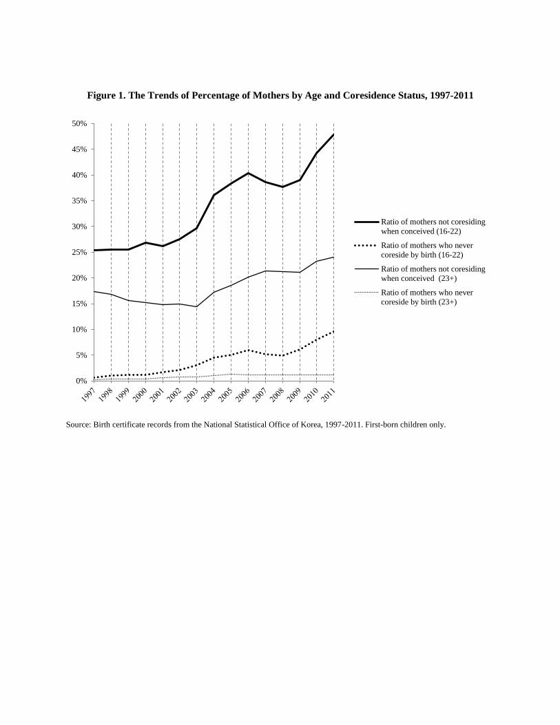
Figure 1. The Trends of Percentage of Mothers by Age and Coresidence Status, 1997-2011

Source: Birth certificate records from the National Statistical Office of Korea, 1997-2011. First-born children only.

0%

5%

10%

15%

20%

25%

30%

35%

40%

45%

50%

Ratio of mothers not coresiding

when conceived (16-22)

Ratio of mothers who never

coreside by birth (16-22)

Ratio of mothers not coresiding

when conceived (23+)

Ratio of mothers who never

coreside by birth (23+)

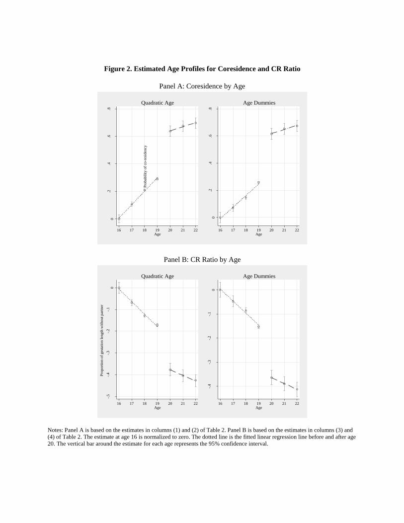
Figure 2. Estimated Age Profiles for Coresidence and CR Ratio

Panel A: Coresidence by Age

Panel B: CR Ratio by Age

Notes: Panel A is based on the estimates in columns (1) and (2) of Table 2. Panel B is based on the estimates in columns (3) and

(4) of Table 2. The estimate at age 16 is normalized to zero. The dotted line is the fitted linear regression line before and after age

20. The vertical bar around the estimate for each age represents the 95% confidence interval.

0.2

.4.6

.8

Pro

bab

ilit

y o

f co

-res

iden

cy

16 17 18 19 20 21 22Age

Quadratic Age

0.2

.4.6

.8

Pro

bab

ilit

y o

f co

-res

iden

cy

16 17 18 19 20 21 22Age

Age Dummies-.

5-.

4-.

3-.

2-.

10

Pro

port

ion

of

ges

tati

on l

eng

th w

itho

ut

par

tner

16 17 18 19 20 21 22Age

Quadratic Age

-.4

-.3

-.2

-.1

0

Pro

port

ion

of

ges

tati

on l

eng

th w

itho

ut

par

tner

16 17 18 19 20 21 22Age

Age Dummies

Table 1. Summary Statistics by Coresidence and Marital Status of Mothers

By coresidence status By marital status

CRB noR RCB Married Unmarried

CR Ratio* 0.36 1.00 0.00 0.12 0.47

[0.26] [0.24] [0.48]

Birth weight (in kilogram) 3.24 3.11 3.21 3.22 3.12

[0.43] [0.47] [0.44] [0.43] [0.47]

Low birth weight 0.033 0.071 0.041 0.038 0.070

[0.179] [0.257] [0.198] [0.192] [0.254]

Premature birth

(gestation weeks < 38) 0.067 0.137 0.080 0.076 0.131

[0.250] [0.344] [0.272] [0.265] [0.338]

Not born in hospital 0.014 0.040 0.018 0.016 0.044

[0.118] [0.196] [0.132] [0.126] [0.206]

Mother’s age 20.92 19.72 20.71 20.81 19.32

[1.24] [1.78] [1.36] [1.29] [1.86]

Boy 0.51 0.52 0.52 0.51 0.52

[0.50] [0.50] [0.50] [0.50] [0.50]

Mother’s education

Less than high school 0.08 0.28 0.16 0.13 0.35

[0.27] [0.45] [0.36] [0.33] [0.48]

High school graduate 0.72 0.60 0.72 0.73 0.56

[0.45] [0.49] [0.45] [0.45] [0.50]

College or higher 0.21 0.12 0.12 0.15 0.09

[0.41] [0.32] [0.32] [0.35] [0.29]

Multiple births 0.005 0.005 0.005 0.005 0.004

[0.07] [0.07] [0.007] [0.07] [0.06]

Number of observations 69,429 7,482 169,467 235,344 11,034

Notes: Standard deviations are reported in square brackets. Mother’s education level is defined by terminal degree or current

enrollment at the time of the birth report. *CR ratio refers to the duration between conception (C) and co-residence (R) out of

total gestation weeks, formally defined in equation (3).

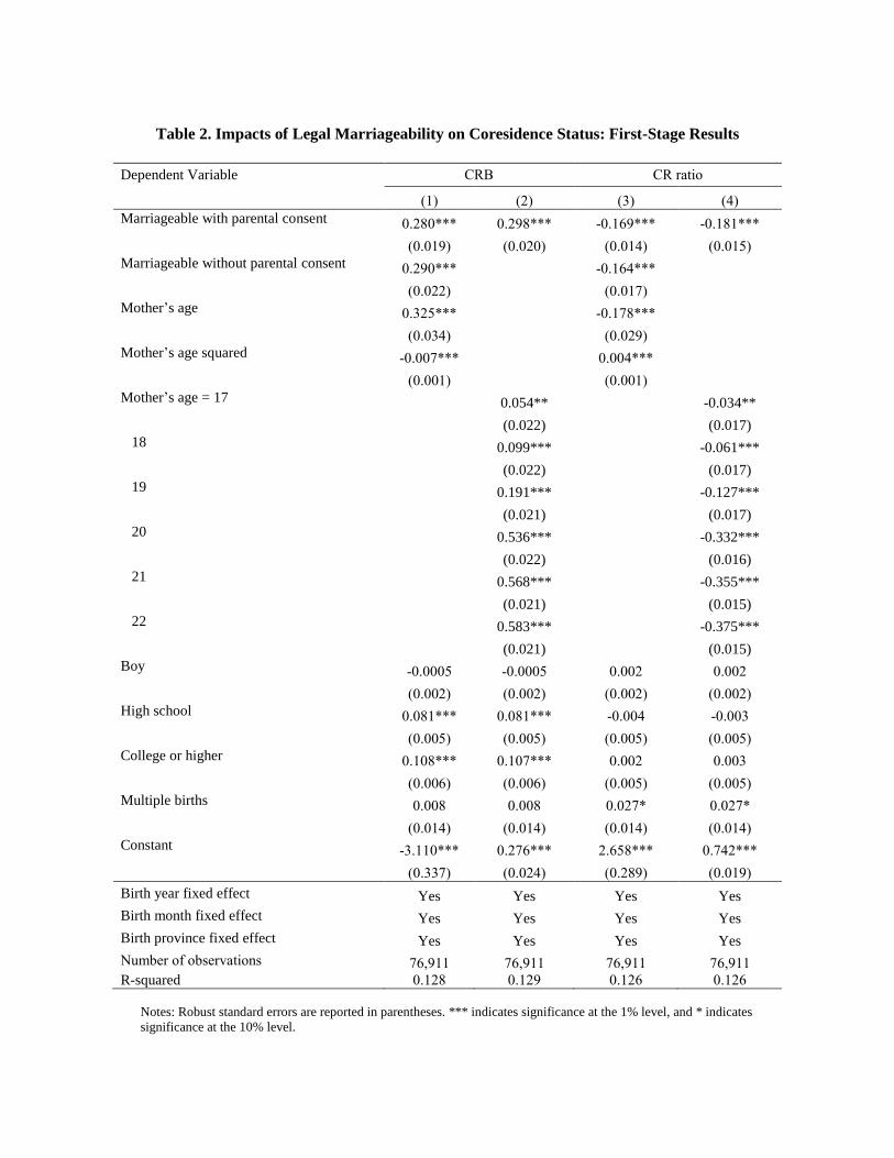
Table 2. Impacts of Legal Marriageability on Coresidence Status: First-Stage Results

Dependent Variable CRB CR ratio

(1) (2) (3) (4)

Marriageable with parental consent 0.280*** 0.298*** -0.169*** -0.181***

(0.019) (0.020) (0.014) (0.015)

Marriageable without parental consent 0.290*** -0.164***

(0.022) (0.017)

Mother’s age 0.325*** -0.178***

(0.034) (0.029)

Mother’s age squared -0.007*** 0.004***

(0.001) (0.001)

Mother’s age = 17 0.054** -0.034**

(0.022) (0.017)

18 0.099*** -0.061***

(0.022) (0.017)

19 0.191*** -0.127***

(0.021) (0.017)

20 0.536*** -0.332***

(0.022) (0.016)

21 0.568*** -0.355***

(0.021) (0.015)

22 0.583*** -0.375***

(0.021) (0.015)

Boy -0.0005 -0.0005 0.002 0.002

(0.002) (0.002) (0.002) (0.002)

High school 0.081*** 0.081*** -0.004 -0.003

(0.005) (0.005) (0.005) (0.005)

College or higher 0.108*** 0.107*** 0.002 0.003

(0.006) (0.006) (0.005) (0.005)

Multiple births 0.008 0.008 0.027* 0.027*

(0.014) (0.014) (0.014) (0.014)

Constant -3.110*** 0.276*** 2.658*** 0.742***

(0.337) (0.024) (0.289) (0.019)

Birth year fixed effect Yes Yes Yes Yes

Birth month fixed effect Yes Yes Yes Yes

Birth province fixed effect Yes Yes Yes Yes

Number of observations 76,911 76,911 76,911 76,911

R-squared 0.128 0.129 0.126 0.126

Notes: Robust standard errors are reported in parentheses. *** indicates significance at the 1% level, and * indicates

significance at the 10% level.

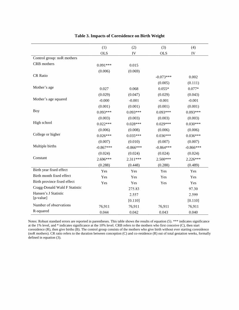
Table 3. Impacts of Coresidence on Birth Weight

(1) (2) (3) (4)

OLS IV OLS IV

Control group: noR mothers

CRB mothers 0.091*** 0.015

(0.006) (0.069)

CR Ratio -0.073*** 0.002

(0.005) (0.111)

Mother’s age 0.027 0.068 0.055* 0.077*

(0.029) (0.047) (0.029) (0.043)

Mother’s age squared -0.000 -0.001 -0.001 -0.001

(0.001) (0.001) (0.001) (0.001)

Boy 0.093*** 0.093*** 0.093*** 0.093***

(0.003) (0.003) (0.003) (0.003)

High school 0.022*** 0.028*** 0.029*** 0.030***

(0.006) (0.008) (0.006) (0.006)

College or higher 0.026*** 0.035*** 0.036*** 0.036***

(0.007) (0.010) (0.007) (0.007)

Multiple births -0.867*** -0.866*** -0.864*** -0.866***

(0.024) (0.024) (0.024) (0.024)

Constant 2.696*** 2.311*** 2.500*** 2.226***

(0.288) (0.448) (0.288) (0.489)

Birth year fixed effect Yes Yes Yes Yes

Birth month fixed effect Yes Yes Yes Yes

Birth province fixed effect Yes Yes Yes Yes

Cragg-Donald Wald F Statistic 275.83 97.30

Hansen’s J Statistic

[p-value] 2.557 2.599

[0.110] [0.110]

Number of observations 76,911 76,911 76,911 76,911

R-squared 0.044 0.042 0.043 0.040

Notes: Robust standard errors are reported in parentheses. This table shows the results of equation (5). *** indicates significance

at the 1% level, and * indicates significance at the 10% level. CRB refers to the mothers who first conceive (C), then start

coresidence (R), then give births (B). The control group consists of the mothers who give birth without ever starting coresidence

(noR mothers). CR ratio refers to the duration between conception (C) and co-residence (R) out of total gestation weeks, formally

defined in equation (3).

Table 4. Impacts of Coresidence on Low Birth Weight (LBW)

(1) (2) (3) (4)

Probit

Bivariate

Probit Probit IV Probit

Control group: noR mothers

CRB mothers -0.026*** 0.008

(0.003) (0.014)

CR Ratio 0.023*** 0.001

(0.002) (0.036)

Mother’s age 0.005 -0.011 0.001 -0.006

(0.011) (0.013) (0.011) (0.016)

Mother’s age squared -0.0002 0.0001 -0.0001 0.0001

(0.0003) (0.0003) (0.0003) (0.0004)

Boy -0.006*** -0.007*** -0.006*** -0.006***

(0.001) (0.001) (0.001) (0.001)

High school -0.003 -0.006** -0.005** -0.005**

(0.002) (0.003) (0.002) (0.002)

College or higher -0.005** -0.010*** -0.008*** -0.008***

(0.002) (0.004) (0.002) (0.002)

Multiple births 0.517*** 0.152*** 0.513*** 0.515***

(0.026) (0.006) (0.026) (0.026)

Birth year fixed effect Yes Yes Yes Yes

Birth month fixed effect Yes Yes Yes Yes

Birth province fixed effect Yes Yes Yes Yes

Cragg-Donald Wald F Statistic 275.83 97.30

Hansen J Statistic

[p-value] 0.261 0.171

[0.610] [0.679]

Number of observations 76,911 76,911 76,911 76,911

Log pseudo-likelihood -11,542 -32,217 -11,538 -25,920

Notes: This table shows the results of equation (5). Marginal effects, evaluated at sample means, are presented. For bivariate

probit, birth month fixed effects are excluded from the estimation equation for coresidence. Robust standard errors are reported in

parentheses. *** indicates significance at the 1% level, and **indicates significance at the 5% level.

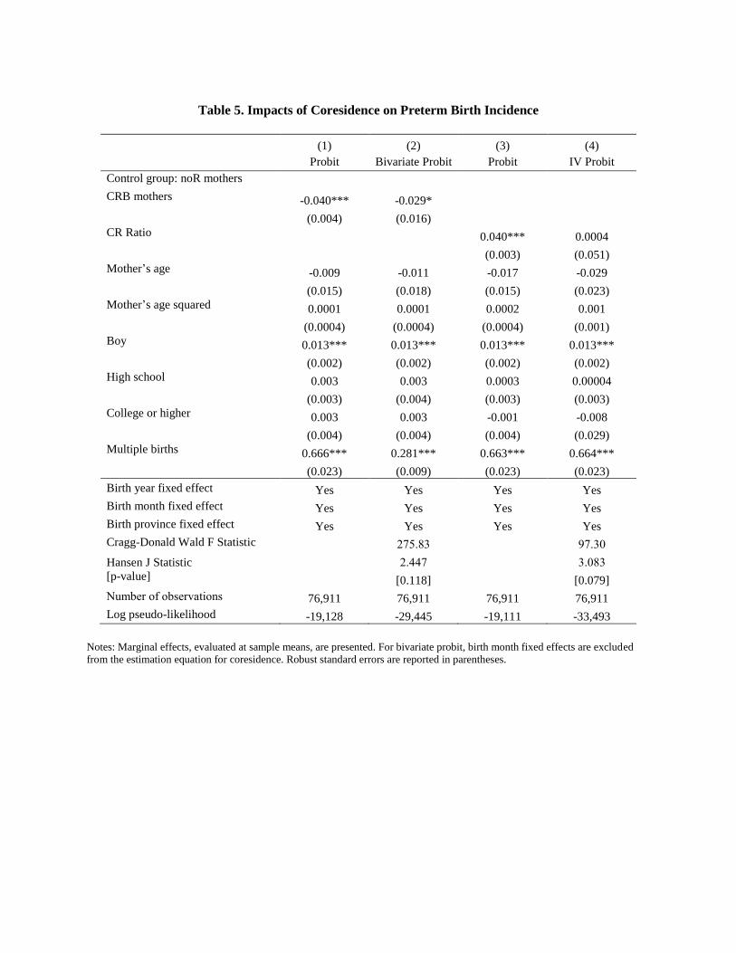
Table 5. Impacts of Coresidence on Preterm Birth Incidence

(1) (2) (3) (4)

Probit Bivariate Probit Probit IV Probit

Control group: noR mothers

CRB mothers -0.040*** -0.029*

(0.004) (0.016)

CR Ratio 0.040*** 0.0004

(0.003) (0.051)

Mother’s age -0.009 -0.011 -0.017 -0.029

(0.015) (0.018) (0.015) (0.023)

Mother’s age squared 0.0001 0.0001 0.0002 0.001

(0.0004) (0.0004) (0.0004) (0.001)

Boy 0.013*** 0.013*** 0.013*** 0.013***

(0.002) (0.002) (0.002) (0.002)

High school 0.003 0.003 0.0003 0.00004

(0.003) (0.004) (0.003) (0.003)

College or higher 0.003 0.003 -0.001 -0.008

(0.004) (0.004) (0.004) (0.029)

Multiple births 0.666*** 0.281*** 0.663*** 0.664***

(0.023) (0.009) (0.023) (0.023)

Birth year fixed effect Yes Yes Yes Yes

Birth month fixed effect Yes Yes Yes Yes

Birth province fixed effect Yes Yes Yes Yes

Cragg-Donald Wald F Statistic 275.83 97.30

Hansen J Statistic

[p-value]

2.447 3.083

[0.118] [0.079]

Number of observations 76,911 76,911 76,911 76,911

Log pseudo-likelihood -19,128 -29,445 -19,111 -33,493

Notes: Marginal effects, evaluated at sample means, are presented. For bivariate probit, birth month fixed effects are excluded

from the estimation equation for coresidence. Robust standard errors are reported in parentheses.

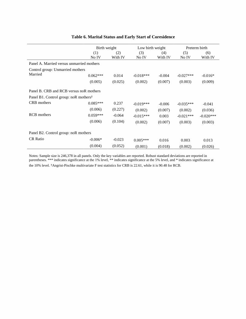
Table 6. Marital Status and Early Start of Coresidence

Birth weight Low birth weight Preterm birth

(1)

No IV

(2)

With IV

(3)

No IV

(4)

With IV

(5)

No IV

(6)

With IV

Panel A. Married versus unmarried mothers

Control group: Unmarried mothers

Married 0.062*** 0.014 -0.018*** -0.004 -0.027*** -0.016*

(0.005) (0.025) (0.002) (0.007) (0.003) (0.009)

Panel B. CRB and RCB versus noR mothers

Panel B1. Control group: noR mothers†

CRB mothers 0.085*** 0.237 -0.019*** -0.006 -0.035*** -0.041

(0.006) (0.227) (0.002) (0.007) (0.002) (0.036)

RCB mothers 0.059*** -0.064 -0.015*** 0.003 -0.021*** -0.020***

(0.006) (0.104) (0.002) (0.007) (0.003) (0.003)

Panel B2. Control group: noR mothers

CR Ratio -0.006* -0.023 0.005*** 0.016 0.003 0.013

(0.004) (0.052) (0.001) (0.018) (0.002) (0.026)

Notes: Sample size is 246,378 in all panels. Only the key variables are reported. Robust standard deviations are reported in

parentheses. *** indicates significance at the 1% level, ** indicates significance at the 5% level, and * indicates significance at

the 10% level. †Angrist-Pischke multivariate F test statistics for CRB is 22.61, while it is 90.48 for RCB.

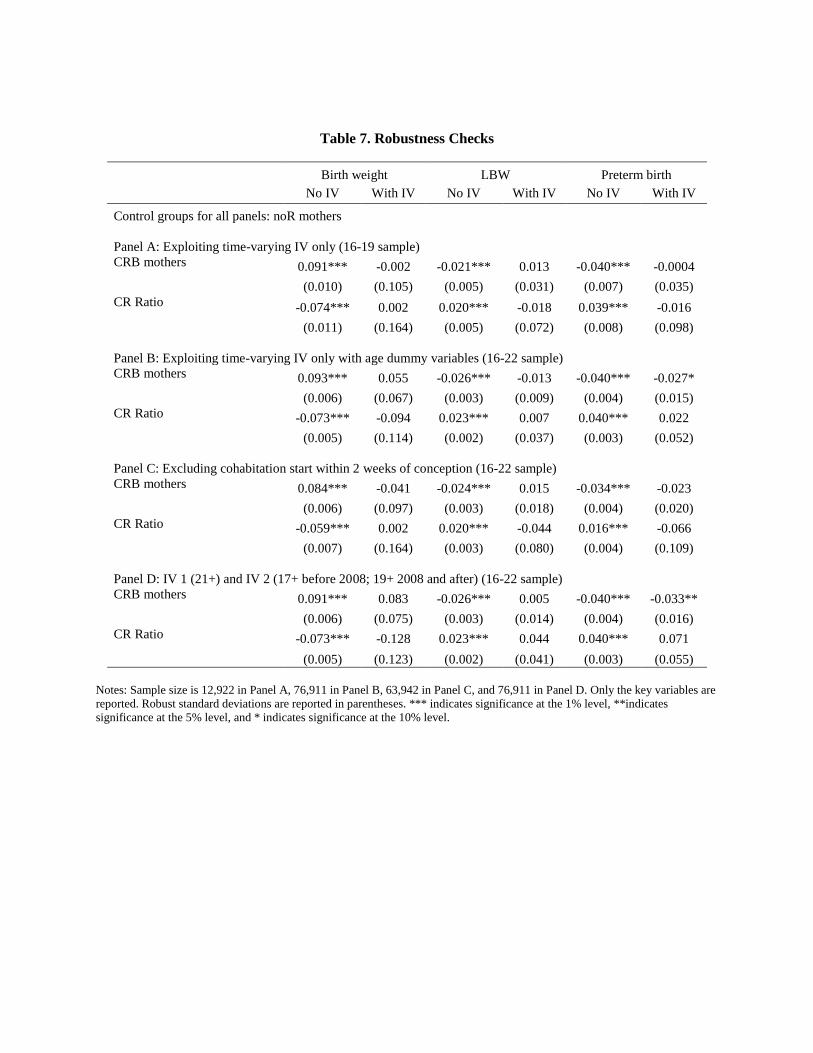
Table 7. Robustness Checks

Birth weight LBW Preterm birth

No IV With IV No IV With IV No IV With IV

Control groups for all panels: noR mothers

Panel A: Exploiting time-varying IV only (16-19 sample)

CRB mothers 0.091*** -0.002 -0.021*** 0.013 -0.040*** -0.0004

(0.010) (0.105) (0.005) (0.031) (0.007) (0.035)

CR Ratio -0.074*** 0.002 0.020*** -0.018 0.039*** -0.016

(0.011) (0.164) (0.005) (0.072) (0.008) (0.098)

Panel B: Exploiting time-varying IV only with age dummy variables (16-22 sample)

CRB mothers 0.093*** 0.055 -0.026*** -0.013 -0.040*** -0.027*

(0.006) (0.067) (0.003) (0.009) (0.004) (0.015)

CR Ratio -0.073*** -0.094 0.023*** 0.007 0.040*** 0.022

(0.005) (0.114) (0.002) (0.037) (0.003) (0.052)

Panel C: Excluding cohabitation start within 2 weeks of conception (16-22 sample)

CRB mothers 0.084*** -0.041 -0.024*** 0.015 -0.034*** -0.023

(0.006) (0.097) (0.003) (0.018) (0.004) (0.020)

CR Ratio -0.059*** 0.002 0.020*** -0.044 0.016*** -0.066

(0.007) (0.164) (0.003) (0.080) (0.004) (0.109)

Panel D: IV 1 (21+) and IV 2 (17+ before 2008; 19+ 2008 and after) (16-22 sample)

CRB mothers 0.091*** 0.083 -0.026*** 0.005 -0.040*** -0.033**

(0.006) (0.075) (0.003) (0.014) (0.004) (0.016)

CR Ratio -0.073*** -0.128 0.023*** 0.044 0.040*** 0.071

(0.005) (0.123) (0.002) (0.041) (0.003) (0.055)

Notes: Sample size is 12,922 in Panel A, 76,911 in Panel B, 63,942 in Panel C, and 76,911 in Panel D. Only the key variables are

reported. Robust standard deviations are reported in parentheses. *** indicates significance at the 1% level, **indicates

significance at the 5% level, and * indicates significance at the 10% level.

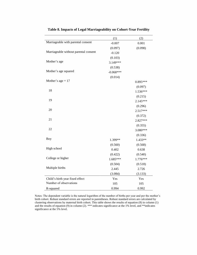
Table 8. Impacts of Legal Marriageability on Cohort-Year Fertility

(1) (2)

Marriageable with parental consent -0.007 0.001

(0.097) (0.098)

Marriageable without parental consent -0.120

(0.103)

Mother’s age 3.149***

(0.538)

Mother’s age squared -0.068***

(0.014)

Mother’s age = 17 0.895***

(0.097)

18 1.536***

(0.215)

19 2.145***

(0.296)

20 2.517***

(0.372)

21 2.827***

(0.355)

22 3.080***

(0.336)

Boy 1.399** 1.433**

(0.560) (0.568)

High school 0.402 0.638

(0.422) (0.540)

College or higher 1.685*** 1.776***

(0.504) (0.518)

Multiple births 2.445 2.726

(3.084) (3.133)

Child’s birth year fixed effect Yes Yes

Number of observations 105 105

R-squared 0.994 0.992

Notes: The dependent variable is the natural logarithm of the number of births per year and per the mother’s

birth cohort. Robust standard errors are reported in parentheses. Robust standard errors are calculated by

clustering observations by maternal birth cohort. This table shows the results of equation (8) in column (1)

and the results of equation (9) in column (2). *** indicates significance at the 1% level, and **indicates

significance at the 5% level.

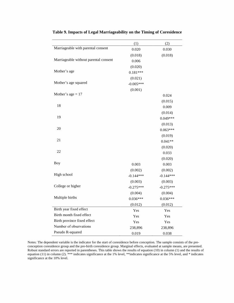
Table 9. Impacts of Legal Marriageability on the Timing of Coresidence

(1) (2)

Marriageable with parental consent 0.020 0.030

(0.018) (0.018)

Marriageable without parental consent 0.006

(0.020)

Mother’s age 0.181***

(0.021)

Mother’s age squared -0.005***

(0.001)

Mother’s age = 17 0.024

(0.015)

18 0.009

(0.014)

19 0.049***

(0.013)

20 0.063***

(0.019)

21 0.041**

(0.020)

22 0.033

(0.020)

Boy 0.003 0.003

(0.002) (0.002)

High school -0.144*** -0.144***

(0.003) (0.003)

College or higher -0.275*** -0.275***

(0.004) (0.004)

Multiple births 0.036*** 0.036***

(0.012) (0.012)

Birth year fixed effect Yes Yes

Birth month fixed effect Yes Yes

Birth province fixed effect Yes Yes

Number of observations 238,896 238,896

Pseudo R-squared 0.019 0.038

Notes: The dependent variable is the indicator for the start of coresidence before conception. The sample consists of the pre-

conception coresidence group and the pre-birth coresidence group. Marginal effects, evaluated at sample means, are presented.

Robust standard errors are reported in parentheses. This table shows the results of equation (10) in column (1) and the results of

equation (11) in column (2). *** indicates significance at the 1% level, **indicates significance at the 5% level, and * indicates

significance at the 10% level.