Embed Size (px)
Citation preview

dJay : Enabling High-density Multi-tenancy for Cloud GamingServers with Dynamic Cost-Benefit GPU Load Balancing
Sergey Grizan
Siberian Federal University
David Chu, Alec Wolman
Microsoft Research
{davidchu, alecw}@microsoft.com
Roger Wattenhofer
ETH Zurich
AbstractIn cloud gaming, servers perform remote rendering on behalf
of thin clients. Such a server must deliver sufficient frame
rate (at least 30fps) to each of its clients. At the same time,
each client desires an immersive experience, and therefore
the server should also provide the best graphics quality pos-
sible to each client. Statically provisioning time slices of the
server GPU for each client suffers from severe underutiliza-
tion because clients can come and go, and scenes that the
clients need rendered can vary greatly in terms of GPU re-
source usage over time.
In this work, we present dJay, a utility-maximizing cloud
gaming server that dynamically tunes client GPU rendering
workloads in order to 1) ensure all clients get satisfactory
frame rate, and 2) provide the best possible graphics qual-
ity across clients. To accomplish this, we develop three main
components. First, we build an online profiler that collects
key cost and benefit data, and distills the data into a reusable
regression model. Second, we build an online utility opti-
mizer that uses the regression model to tune GPU workloads
for better graphics quality. The optimizer solves the Multi-
ple Choice Knapsack problem. We demonstrate dJay on two
high quality commercial games, Doom 3 and Fable 3. Our
results show that when compared to a static configuration,
we can respond much better to peaks and troughs, achieving
up to four times the multi-tenant density on a single server
while offering clients the best possible graphics quality.
Categories and Subject Descriptors C.2.4 [Computer-Communication Networks]: Distributed Systems—Distributed
Applications; I.6.8 [Simulation and Modeling]: Types of
Simulation—Gaming
Keywords GPU management; server load balancing
Permission to make digital or hard copies of all or part of this work for personal orclassroom use is granted without fee provided that copies are not made or distributedfor profit or commercial advantage and that copies bear this notice and the full citationon the first page. Copyrights for components of this work owned by others than ACMmust be honored. Abstracting with credit is permitted. To copy otherwise, or republish,to post on servers or to redistribute to lists, requires prior specific permission and/or afee. Request permissions from [email protected].
SoCC ’15, August 27–29, 2015, Kohala Coast, HI, USA.Copyright c© 2015 ACM 978-1-4503-3651-2/15/08. . . $15.00.http://dx.doi.org/10.1145/2806777.2806942
1. IntroductionGaming is popular. Recently, cloud gaming — where dat-
acenter servers host game application instances and clients
merely transmit UI input and display output (e.g. frame
buffers) from servers — has emerged as an interesting alter-
native to traditional client-side execution. Sony’s PlaySta-
tion Now, Nvidia’s GRID and Amazon’s AppStream are
among the cloud gaming services available to consumers to-
day [1, 3, 4].
Cloud gaming offers several advantages. Client-side sys-
tem configuration and platform compatibility issues are
eliminated, alleviating a long-standing headache of tradi-
tional non-console gaming and mobile device gaming. In
addition, upgrading datacenter servers with better hardware
is far easier than redeploying hardware to clients. Further-
more, players can select from a vast library of games and
instantly play any of them.
However, cloud gaming faces several technical chal-
lenges that are not unfamiliar to other cloud service providers:
latency, bandwidth and multi-tenancy [6]. Previous work has
looked at reducing cloud gaming’s latency and bandwidth
costs [8, 20]. In this work, we tackle multi-tenancy: how can
a server host as many players as possible? Multi-tenancy’s
importance is underscored by the lessons of one early cloud
gaming pioneer, which failed in part because it could only
support one client per server, thereby making a large and
ultimately unsustainable investment in server farms [13].
At first, it might appear that the same isolation and virtu-
alization support that has served traditional hosted services
well would suffice for multi-tenant gaming. However, cloud
gaming multi-tenancy is challenging and distinct from tradi-
tional datacenter multi-tenancy because games exhibit three
unique properties.
• GPU-Centric Workload: Graphics rendering is heavily
reliant upon the GPU. System resources such as disk,
system memory and CPU are often underloaded.
• Continuous Deadlines: Acceptable gaming interactiv-
ity requires continuous frame processing of at least 30
Frames Per Second (FPS) for the whole session. Play-
ers become dissatisfied when frame rates fall below 30
FPS [7].
58
• Adjustable Visual Quality: Games typically expose
many optional graphical effects (e.g., anti-aliasing, tex-
ture details, shadows) that produce higher quality graph-
ics. Provided at least 30 FPS, players prefer the highest
possible visual quality.
Naıvely running multiple tenants concurrently on a server
can pose grave shortcomings. The load generated by one in-
stance can squeeze out another instance, resulting in missed
deadlines, low or erratic frame rates and an unplayable expe-
rience. Even the load generated by a single instance exhibits
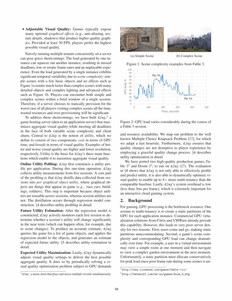
significant temporal variability due to scene complexity: sim-
ple scenes with a few basic objects and no effects such as
Figure 1a render much faster than complex scenes with many
detailed objects and complex lighting and advanced effects
such as Figure 1b. Players can encounter both simple and
complex scenes within a brief window of a single session.
Therefore, if a server chooses to statically provision for the
worst case of all players visiting complex scenes all the time,
wasted resources and over-provisioning will be significant.
To address these shortcomings, we have built dJay,1 a
game hosting server (akin to an application server) that max-
imizes aggregate visual quality while meeting all deadlines
in the face of both variable scene complexity and client
churn. Central to dJay is the notion of utility, which we
define to consist of two components: cost in terms of GPU
time, and benefit in terms of visual quality. Examples of bet-
ter and worse visual quality are higher and lower resolution,
respectively. Utility is the basis for dJay’s three main func-
tions which enable it to maximize aggregate visual quality.
Online Utility Pofiling: dJay first constructs a utility pro-
file per application. During this one-time operation, dJay
collects utility measurements from live sessions. A core part
of the profiling is that dJay distills data collected from ses-
sions into per graphical object utility, where graphical ob-
jects are things that appear in game (e.g., race cars, build-
ings, soldiers). This step is important because object utili-
ties are reusable across sessions, whereas session utilities are
not. The distillation occurs through regression model con-
struction. §4 describes utility profiling in detail.
Future Utility Estimation: After the regression model is
constructed, dJay actively monitors each live session to de-
termine whether a session’s utility will change significantly
in the near term (which can happen often, for example, due
to scene changes). To produce an accurate estimate, dJay
queries the game for a list of game objects, and applies the
regression model to the objects, and generates an estimate
of expected future utility. §5 describes utility estimation in
detail.
Expected Utility Maximization: Lastly, dJay dynamically
adjusts visual quality settings to deliver the best possible
aggregate quality. It does so by periodically solving a vi-
sual quality optimization problem subject to GPU demands
1 dJay : a music artist that plays and mixes multiple records simultaneously.
(a) Simple Scene (b) Complex Scene
Figure 1: Scene complexity examples from Fable 3.
0102030405060708090
100
0 100 200 300 400 500
GPU
load
, %
Time, seconds
(fig. 1a)
(fig. 1b)
Figure 2: GPU load varies considerably during the course of
a Fable 3 session.
and resource availability. We map our problem to the well
known Multiple Choice Knapsack Problem [17], for which
we adapt a fast heuristic. Furthermore, dJay ensures that
quality changes are not disruptive to player experience by
employing a graceful quality change process. §6 describes
utility optimization in detail.
We have ported two high-quality production games, Fa-
ble 32 and Doom 33, to run on dJay (§7). The evaluation
in §8 shows that dJay is not only able to effectively profile
and predict utility, it is also able to dynamically optimize vi-
sual quality to enable up to 4× more multi-tenancy than the
comparable baseline. Lastly, dJay’s system overhead is low
(less than 3ms per frame), which is extremely important for
an interactive cloud gaming system.
2. BackgroundFor gaming, GPU processing is the bottleneck resource. One
avenue to multi-tenancy is to create a static partitions of the
GPU for each application instance. Commercial GPU virtu-
alization solutions from Citrix and VMWare already provide
this capability. However, this leads to very poor server den-
sity for two reasons. First, users come and go, making static
partitions unaccommodating. Second, a game’s scene com-
plexity and corresponding GPU load can change dramati-
cally over time. For example, a user in a virtual environment
may view a simple room at one moment and then navigate
to view a complex garden environment in the next moment.
Unfortunately, a static partition must allocate conservatively
for peak load since poor frame rate during some scenes is un-
2 http://www.lionhead.com/games/fable-iii/3 http://bethsoft.com/en-us/games/doom_3_bfg
59

satisfactory. This means during any non-peak load — which
occur frequently — GPU cores sit idle. Figure 2 shows that
for a typical application, much GPU capacity remains idle
for much of the time. The timespans of high utilization and
low utilization correspond to scenes like Figure 1b and Fig-
ure 1a, respectively. This waste leads to inefficient opera-
tions on the part of the service providers.
We observe that almost all games provide the capabil-
ity to tune rendering settings. Common examples of render-
ing settings include screen resolution, antialiasing, lighting
model complexity, enabling or disabling shadows, and tex-
ture detail. Developers offer these knobs because end user
machines vary greatly in capability. With traditional thick
clients (no cloud gaming), a user with a powerful machine
can enable many advanced rendering settings whereas a user
with a modest machine can tone down settings in order to
maintain a responsive FPS. A speed of 30 FPS is widely re-
garded as the threshold for a playable experience. Therefore,
we treat its inverse, 33ms per frame, as the maximum per-
missible frame time. Since frame rates above 30 FPS have
marginal benefits [7], in this work we consider any frame
time 33ms or below equally acceptable.
We leverage the rendering settings that titles already ex-
pose as the means to trade off better visual quality for lower
resource utilization. Games commonly contain a fixed num-
ber of preset rendering settings such as High, Medium and
Low, which in turn map to various settings for individ-
ual rendering parameters (e.g., High gives 16× antialiasing,
maximum texture detail, etc.). It is worth noting that changes
in rendering settings are strictly visual enhancements and
have no bearing on game semantics. Therefore, we are free
to alter rendering settings at any time without side effects on
game logic.
We also introduce the Structural Similarity (SSIM) score,
a standard criteria of the video compression community
used to quantify the perceived loss in video quality between
a pristine image f ∗ and a distorted version of the image,
f [26]. For example, the images f ∗ and f might represent
the same scene rendered with a High setting and a Medium
(or Low) setting, respectively. The function SSIMf ∗( f ) takes
a real value in [0,1] where a lower values indicates lower fi-
delity to the pristine image. By definition, SSIMf ∗( f ∗) = 1
and SSIMf ∗( f ) = 0 when f is random noise. While SSIM
is not perfect at reflecting human subjective assessment of
quality, it is more accurate than alternative measures such
as SNR and PSNR, and maps reasonably to the standard
subjective user-study based measure for video quality, Mean
Opinion Score [26].
3. ApproachGiven a fixed budget of 33ms per frame, the questions we
aim to address are:
• Cost: What rendering settings are feasible?
• Benefit: Among the feasible, which setting is best?
These turn out to be challenging questions for two reasons.
First, the feasible combinations depend greatly on the GPU
cost of the workload at hand. As previously noted, scene
complexity can change anytime. A rendering setting that
is feasible for the current scene in the game may be too
expensive for other scenes in the game. Second, among those
feasible rendering settings, the “best” can differ depending
upon the scene. For example, consider the two renderings
of the same arch scene shown in Figure 3. There are very
noticeable differences in the landscape between the high
quality and low quality renderings. In contrast, the high and
low quality renderings of a coastal scene shown in Figure 4
look very similar. Therefore, we cannot assume that the
benefits of more sophisticated rendering apply uniformly to
all scenes.
Figure 5 illustrates the architecture of dJay by which
we resolve these questions about cost and benefit. We next
describe its main pieces.
3.1 Measuring CostIn order to understand which combinations of rendering set-
tings are feasible, we build profiles of each app’s frame
time under different rendering settings. However, frame
time alone lacks context; given a rendering setting, we lack
any notion of what may be causing higher or lower frame
time. Without additional context, we are limited to attribut-
ing (high) frame times to coarse app-level granularity. This
worst case estimate attains no better resource utilization than
conservative static partitioning.
Ideally, we ought to map frame time to relevant in-game
context. We conjecture that graphical objects can serve as
useful context because they can have a large impact on frame
time. As a concrete example, graphical objects in Fable 3
include castles, houses, enemies and non-player characters,
to name just a few. Graphical objects are created at the
discretion of the app developers and a typical game contains
hundreds to thousands. Since a castle object is graphically
much more complex than a house object, we aim to attribute
a higher GPU cost to castles than to houses. Suppose for
every frame, the game provides us the active object list(AOL), the list of graphical object types used to render the
frame. By mapping cost to graphical objects, we can later
estimate a cost for a novel scene based on the graphical
object types it contains. dProf shown in Figure 5 is the
component that measures costs and performs the mapping
of costs to graphical objects. We use statistical regressionmodels to determine the cost-to-object mapping (§4).
3.2 Measuring BenefitIn order to objectively assess “best,” we use SSIM and com-
pare rendering settings as follows for a given scene. Suppose
we generate the pristine image f ∗ with rendering settings R∗where R∗ is the setting with every optional rendering setting
dialed to maximum quality. Let R1 and R2 be two rendering
settings and let f1 and f2 be the images generated by them,
60

(a) High Quality (b) Low Quality
Figure 3: Major differences between High and Low Quality.
(a) High Quality (b) Low Quality
Figure 4: Minor differences between High and Low Quality.
dProf: utility profiler
dIce: concurrent executionSession #28
(master instance)Session #28
(slave instance)
per frame: <rendering setting, frame time, SSIM, Active Object List (AOL)>
Online Profiling
Session #913 Session #914 Session #915 Session #916
dOpt: utility optimizationdEst: utility estimation
Online Utility Maximization
per frame: <Potential Object List (POL)>rendering setting
Regression Model<rendering setting, object id, cost, benefit>
Figure 5: The dJay architecture shows the relationship of various components, all of which run online. Blue arrows represent
measurement whereas red arrows represent control.
respectively. We say R1 > R2 if SSIMf ∗( f1) > SSIMf ∗( f2).However, comparing the SSIM of two existing frames is in-
sufficient to tell us about the SSIM of a novel frame that we
encounter in the future.
As with frame time, we wish to generalize SSIM beyond
a single frame. Therefore, we employ an approach for SSIM
that is similar to the approach that we employed for frame
time. dProf also uses statistical regression to map the SSIM
of a frame to the SSIM contribution of graphical objects in
the frame, thereby deriving a per-object “benefit” measure-
ment (§4). These benefit values are opaque in that they can-
not be interpreted as SSIM per se. We show how they are
used next.
3.3 Estimating Future UtilityWith regression models constructed, our next task is to apply
the models at runtime to estimate the utility — the benefit-
to-cost ratio — of upcoming scenes for various rendering
settings. This is performed by dEst. Two aspects worth
elaboration are 1) why we work on upcoming scenes, and
2) how we estimate the utility of various rendering settings.
First, we focus on upcoming scenes (as opposed to past
scenes or the current scene) because upcoming scenes are
the ones for which we still have the opportunity to adjust
rendering settings. The main challenge is to identify upcom-
ing scenes in a reasonable way. We introduce the notion of a
potential object list (POL). The POL consists of those game
object types that are likely to be encountered by the player
within a short time horizon. For example, a castle just be-
yond the player’s field of view is a good candidate for the
POL. dEst receives POL updates from the game dynami-
cally.
Second, we estimate utility with respect to both current
and alternative rendering settings. Estimation for one ren-
dering setting consists of using the regression model to per-
form a statical inference. dEst makes the estimate for each
rendering setting to arrive at a collection of utilities, one for
each rendering setting.
3.4 OptimizationdOpt takes the future utilities computed by dEst for all ses-
sions, computes a utility-maximizing assignment of render-
ing settings to sessions, and then propagates the new render-
ing settings to the corresponding sessions. The utility maxi-
mization problem nicely maps to the Multiple Choice Knap-
sack Problem, for which polynomial time approximations
are available [17, 22]. However, we choose a simpler greedy
heuristic because dOpt must complete its online decision
making very quickly. In addition, we incorporate a limited
form of hysteresis into our heuristic such that visual qual-
ity changes are gracefully made when possible, and quickly
enacted when necessary.
3.5 RequirementsFor dJay to work as described above, we require that:
61

1. An instance can report the AOL and POL for every frame.
2. An instance can change rendering settings dynamically.
Fortunately for Requirement 1, the AOL and POL are al-
ready maintained as part of standard rendering data struc-
tures like Octrees and k-d trees [10]. How an app maintains
this data structure internally (tree, nested, graph, etc.) is an
internal design decision. We simply require these be exposed
to dJay as a generic flat namespace list. It is even permis-
sible for the app to pass lists with extra or missing objects.
This does not affect correctness; it will only impact how well
dJay can optimize the density of the server. Therefore, it is
straightforward for a developer to expose the AOL and POL
to dJay; just pass the already-in-use rendering data struc-
tures as lists. For Requirement 2, games typically permit ad-
justment of rendering settings in-game, so it is straightfor-
ward.
4. Online Utility ProfilingWe next describe the detailed operation of dProf.
4.1 Building Game Object ProfilesFrom a session s with a fixed rendering setting r, dEst
screen captures a set of uncompressed frames, f sr1 , f sr
2 , ..., f srN .
Due to storage constraints, it may be a subset of the frames
that the user actually sees during the session. From each
frame f sri , we measure its cost in terms of GPU frame time,
csri , and its benefit in terms of SSIM bsr
i . We also require that
the game report the frame’s AOL, which is a list of graphical
objects, Gsri = {gsr
i j} where j is the unique ID of each game
object type (e.g., castle type 42) and gsri j represents the
number of game objects of type j in frame i of session swith rendering setting r.
In order to build a per-game object profile, we construct
a system of equations as follows.
∑j
wbjg
sri j = bsr
i ∀i,s,r
∑j
wcjg
sri j = csr
i ∀i,s,r
where wcj and wb
j are the weights for cost and benefit, respec-
tively. We use a least squares method to determine the un-
known weights. Weights essentially encode per-game object
profile information. Note that a game object whose impact
on cost and/or benefit is high will naturally be assigned a
higher weight. Note also that measurements from additional
sessions simply result in more equations, leading to more re-
fined weightings. Alternative models such as nonlinear and
neural networks are also feasible. We tried some of these
and found the simple linear model to work surprisingly well
in practice. Lastly, weights need not be pinpoint precise as
long as they are informative enough to guide cost-benefit de-
cisions.
0
0.005
0.01
0.015
0.02
0.025
0
1000
2000
3000
4000
5000
6000
guardian skybridge zombie1 zombie2 hellchain elevator
Pred
icted
cost
, uni
tless
Vert
ex co
unt
Vertex count Predicted cost
Figure 6: Vertex count correlates well with graphical ob-
ject cost. Therefore, a coarse filter eliminates unimportant
objects by their vertex count. Shown here is a small ran-
dom sampling of over 130 Doom 3 objects. The names
“guardian,” “skybridge,” etc. are the original object names
given by the Doom 3 developers.
4.2 Deterministic Instance Concurrent ExecutionWhile measuring GPU cost is straightforward, measuring
SSIM benefit is more nuanced. Recall that in §3.2 we in-
troduced the function SSIMf ∗i ( fi) where some frame fi is
evaluated against a pristine f ∗i . A key question is how to
obtain f ∗i . To accomplish this, we employ deterministic in-stance concurrent execution (dIce) shown in Figure 5. The
essential idea is to run two instances — a master and a
slave — of the same game concurrently. The instances dif-
fer only in their rendering settings such that the master pro-
duces f ∗1 , f ∗2 , ..., f ∗N and the slave produces f1, f2, ..., fN . The
instances are identical in all other respects: the instances start
in the same initial state, receive the same user input during
the session and process the input deterministically to arrive
at new intermediate states.
A key requirement of the app is that the app should act
deterministically given user input. Previous work has shown
that modern games can be modified in a generic way (e.g.,
converting getTime() calls to return deterministic values
based on a fixed hash seed) to achieve the required input
determinism [8]. dIce pipes user input to both concurrent
instances. The two instances respond deterministically to the
input, differing only in the visual quality of their rendered
output.
Since profiling requires running an extra slave for every
master, we recommend running profiling during quiescent
periods such as 1) during new game onboarding where user
access to the new game is rate limited, and 2) during diurnal
troughs in utilization (e.g., 5am in the morning) when the
service experiences light utilization.
4.3 Object FilteringWhile the per-object profile construction described above
works, it has the potential to create performance issues, es-
pecially if the app passes large lists of graphical objects to
dProf at every frame. To mitigate this issue, we prune the
62

AOL with two filters as follows. First, we coarsely filter the
objects by their vertex count, which is the number of ver-
tices in the object’s 3D representation. Objects that are more
expensive to render tend to have more vertices. Figure 6 il-
lustrates this relationship by showing the tight correlation
between an object’s vertex count and the object’s predicted
cost, wcj. We prune objects whose vertex count is below a
threshold εv. Second, we finely filter the objects by their cost
and benefit weights. The reason that a second level of filter-
ing is necessary is because the object list may still be too
large with just coarse-grained vertex-based filtering. In or-
der to filter by weights, we first construct an initial regres-
sion model with only vertex-based filtering to arrive at some
initial weights. We then filter object type j if either cost or
benefit weight is less than εw. Finally, we construct a new re-
gression model with the remaining objects, arriving at final
weights wbj and wc
j. We have empirically found setting εv to
100 vertices and εw to 0.0001 to work well in practice.
5. Future Utility EstimationNext, dEst uses the weights of the linear regression from
dProf to forecast upcoming cost and benefit. However, we
do not have exact information about future objects since
these are dependent upon the user’s upcoming actions which
are obviously not known. Instead, we use the POL Gsri =
{gsri j}, that are likely to be visible within a short time horizon.
Its notation mirrors that of G: i is the frame number and jis the unique id of the game object. We rely on the game
to provide updates of G to dEst, just like we relied on the
game to provide G to dProf. G only needs to be a guess, not
exact; better guesses lead to more accurate utility estimates.
Providing G is also straightforward for game developers in
practice, as we discussed in §3.5.
In order to estimate upcoming cost csri and benefit bsr
i for
Gsri , we apply the regression model as follows.
bsri = ∑
jwb
j gsri j
csri = ∑
jwc
jgsri j
Cost and benefit are calculated for every frame, which is
feasible since the calculation is very fast.
6. Expected Utility MaximizationFinally, dOpt uses the estimated future utilities to decide on
the visual quality for each session. If costs are expected to
rise, dOpt should downgrade the sessions that suffer little
quality drop but return significant resource savings. Con-
versely, if costs are expected to fall, dOpt should upgrade the
session that gets the most visual quality improvement from
the extra resources newly available. In addition, dOpt should
gracefully change visual quality when possible so that visual
quality changes are not too abrupt for users.
6.1 Optimization Problem and Initial AssignmentThe task is to assign rendering settings to each active session.
We choose to make the assignment such that the aggregate
utility is maximized. Other optimization objectives (such as
maximizing the minimum utility, maximizing fairness, etc.)
are also interesting and we leave them for future work.
From dEst, we have a set of utilities U = {(bsr, csr)},
each of which corresponds to an active session s and render-
ing setting r pairing (we drop the per-frame subscript i since
we only discuss a single time step). The objective function
is to maximize the aggregate expected utility:
Maximize ∑s
∑r
xsrbsr (1)
where xsr is an indicator variable that is 1 if rendering setting
r is chosen for session s and is 0 otherwise. The constraints
are that the total expected cost should be less than the min-
imum acceptable frame time, 33ms, and that each session
should be assigned a rendering setting:
∑s
∑r
xsrcsr < 33ms (2)
∑r
xsr = 1 ∀s (3)
This formulation is a classic variation of the knapsack
problem, known as the multiple choice knapsack problem
(MCKP) [22]. It is NP-hard. We employ a greedy heuris-
tic for MCKP which is inspired by the heuristic presented
in [17]. The idea behind the heuristic is to transform MCKP
into a version of the regular knapsack problem, and apply the
standard greedy solution of the regular (non-multiple choice)
knapsack problem. The key intuition is that we enforce ev-
ery session to have at least some rendering setting assigned
by first assigning all sessions to the lowest rendering setting.
Some residual capacity less than 33ms may be left over for
upgrading some sessions to higher rendering settings. We
then rank all the remaining (bsr, csr) pairs by their utilities
in descending order. However, rather than ranking by ab-
solute utility, we rank by marginal utility, which we define
as the increase in utility of one rendering setting over the
least costly rendering setting of the same session. That is,
the marginal utility is:
usr =bsr − bsq∗
csr − csq∗
q∗ = argminq
csq
Finally, we iteratively pick the top ranked candidate until we
run out of residual capacity. Whenever we pick a candidate
that belongs to session s, we simultaneously excise all other
pairs belonging to s from the ranked list. Our heuristic differs
from that of [17] in that they are willing to tolerate exceeding
the capacity for sake of a solution that is closer to optimal
whereas we are not.
63

Rendering Setting
s = 1 LO ME HI
r = 1 r = 2 r = 3
bsr 0.7 0.8 0.95
csr 2 5 29
(a) Session 1
Rendering Setting
s = 2 LO ME HI
r = 1 r = 2 r = 3
bsr 0.9 0.94 0.96
csr 10 14 15
(b) Session 2
Table 1: An example of two sessions and their correspond-
ing cost and benefits for three rendering settings: LO(W),
ME(DIUM) and HI(GH). The dOpt heuristic identifies ME
and HI for Session 1 and 2, respectively, as explained in the
text.
As an illustration, consider the following example shown
in Table 1 with two sessions and three rendering settings.
The residual cost is 33− 2− 10 = 21. The ranked utilities
are: u1,2 = 0.13 , u2,3 = 0.06
5 , u2,2 = 0.044 and u1,3 = 0.25
27 . We
first pick u1,2 which reduces the remaining frame time to
21−3 = 18. We also remove u1,3 from the list. We then pick
u2,3 which reduces the remaining frame time to 18−15 = 3.
We also remove u2,2 from the list. At this point, no more
candidates remain in the list so the heuristic terminates.
The benefit of the greedy heuristic is that it is both simple
and fast: it runs in time O(n logn) due to the need to sort,
where n is the number of sessions times the number of
rendering settings. Speed is of particular importance because
the heuristic is responsible for online decision making.
6.2 Graceful Change During Normal OperationWe run the heuristic once per epoch, where an epoch is five
frames. The cost and benefit used are the average cost and
benefit over the last epoch. However, dynamically changing
rendering settings arbitrarily can be too abrupt, even once
per epoch. A rendering setting that changes from one ex-
treme of high quality to the other extreme of low quality
could be easily noticed by the user. We protect against abrupt
changes by only permitting rendering settings that are one
level higher or one level lower than the current rendering
setting, in addition to staying at the same rendering setting.
We implement this change by modifying the above MCKP
heuristic as follows. At epoch t, instead of initializing the
heuristic by setting all sessions to the lowest rendering set-
ting, we set all sessions to their rendering settings deter-
mined in epoch t − 1. If the residual frame time is greater
than zero, we have the chance to upgrade some rendering set-
tings as before. However, instead of considering all possible
rendering settings in the ranking, we only consider those ren-
dering settings that are one level higher than the current set-
ting. We pick top ranked utilities from the list as before. Con-
tinuing from the example in Table 1, suppose in Epoch 1 we
have made the selections of rendering setting 2 for session
1 and rendering setting 3 for session 2 as discussed above.
Then in Epoch 2, we only consider rendering setting 3 for
session 1 (as long as costs are equal or less than before). If in-
stead the residual capacity is less than zero (indicating costs
are greater than before), we are in the situation of needing
to downgrade one or more session’s rendering settings. We
then construct a ranked list of marginal utilities in ascending
order, but this time only for those rendering settings that are
one level less than the current settings. We iteratively pick
the top rank from this list until the cost is lowered enough
to satisfy the frame time budget. Taking again the example
in Table 1, suppose Epoch 1 is assigned as discussed previ-
ously, but this time in Epoch 2, all the costs double such that
the residual frame time is now 33− 5× 2− 15× 2 = −7.
The ranked list is then u1,1 = −0.1−6 and u2,2 = −0.02
−2 . In the
first iteration, session 1 is downgraded to rendering setting 1,
leaving −7−−6 =−1 residual frame time. in the next itera-
tion, session 2 is downgraded to rendering setting 2, leaving
−1−−2 = 1 residual frame time.
It is possible that by limiting rendering setting increases
to only one level higher, residual frame time may be wasted
which otherwise might be spent toward an even higher ren-
dering setting. Similarly, it is also possible that by limiting
setting decreases to only one level lower, the total frame time
may still exceed 33ms (i.e., negative residual frame time)
whereas considering all possible rendering setting decreases
may reveal setting(s) that achieve the 33ms target. In prac-
tice, we found that dampening changes is useful because 1)
it minimizes abrupt changes that can distract users, and 2)
if a better setting exists that is more than one step away, we
can still converge to it eventually in future epochs.
It may be the case that we are unable to converge to 33ms
even after several epochs. For this case, we use a two part
fallback solution, called Warning and Critical. dOpt triggers
the Warning condition when the total frame time is between
33ms and 40ms for more than 200 epochs, and triggers the
Critical condition when the total frame time is more than
40ms for more than one epoch. If either Warning or Critical
condition is triggered, all rendering settings are reassigned as
described in §6.1. Critical is usually indicative of a session
permanently transitioning from a scene with low complexity
to a scene with high complexity, in which case we ought
to downgrade right away to maintain a playable experience
for all clients. Warning is afforded a longer interval since
there can be many ephemeral instances where the utilization
spikes briefly.
6.3 Managing Session ChurnUser churn entails both starting and ending sessions. When
a session ends, resources are freed up. We handle this case
just as described for normal operations in §6.2; over one
or more epochs, the remaining sessions will start to use up
the newly freed resources. When a session starts, we take a
two step approach. First, we try to add the new session at
the highest possible rendering setting that fits in the residual
frame time. In a fully loaded system, this often means that
the new session can only be added at the lowest rendering
system, if at all. If this fails (due lack of frame time budget),
64

we then take a more drastic approach of reinitializing all
rendering settings for all sessions as described in §6.1. There
can be cases where even setting every session to the lowest
rendering setting does not satisfy the 33ms budget. This
indicates an admission control failure which we discuss in
§10.
7. ImplementationTo prototype dJay we modified open source Doom 3 (origi-
nally 366,000 lines of code) and Fable 3 (originally 959,000
lines of code) to interface with dProf, dIce, dEst and
dOpt components. Modifications to the games was done via
source code; dProf, dEst and dOpt were implemented as
standalone console processes. The number of modified lines
of code was 500 and 300 for Fable 3 and Doom 3, respec-
tively. All instances run in the same host OS, Windows 8, be-
cause the two apps are written for the Windows platform but
the Windows Hypervisor does not support high performance
GPU virtualization. Other hypervisors such as VMWare and
Citrix do not have this limitation. As a result, we rely on
the host OS’s and GPU device driver’s core scheduling and
memory management mechanisms, neither of which makes
provisions for real-time guarantees, let alone while multi-
plexing the GPU. Therefore, our implementation provides a
conservative reference point in terms of performance gains
possible. Another limitation is that dJay only supports run-
ning one game type (either Fable 3 or Doom 3) at a time;
future work includes load balancing across disparate apps at
once on the same server.
We extended Doom 3 and Fable 3 to invoke the dJay
API where appropriate. The API requires games to receive
rendering setting change commands. The API also requires
games to provide the following data for each in-game frame:
current frame number, frame time, frame buffer, the AOL
and the POL. The data is pulled by the API rather then
pushed by the game to ensure minimum impact on the game
performance. The data being pulled depends on the mode of
operation: profiling or optimization.
7.1 Profiling modeIn profiling mode, the user plays normally on the best render-
ing settings while dJay records every frame’s frame num-
ber, AOL, frame time and frame buffer into a file. Note that
the largest item in this set, the frame buffer, is already being
transferred to the encoder for streaming to the thin client and
dJay merely needs to fork a copy. We modified each game
to save the AOL as an array of object identifiers to a region
of memory shared between the game instance and dJay. For
both Doom 3 and Fable 3, we use the game’s preexisting in-
ternal visible objects data structure as the basis for the AOL.
Coarse-grained object filtering by vertex is implemented as
part of the conversion from internal data structure to AOL.
In order to support deterministic concurrent execution,
we first save the client’s input stream to a buffer. When avail-
able, we take advantage of the fact that games sometimes
support “replay mode” (aka “spectator mode”) to replay the
input stream in a separate instance of the same game at a dif-
ferent rendering setting. During replay mode, we also collect
every frame’s frame number, AOL, frame time and frame
buffer as before. Doom 3 has replay mode built-in. Fable 3
does not have replay mode built-in so we implemented (de-
terministic) replay ourselves by adding the following com-
mand line options: -capture causes the game to dump key-
board, mouse and joystick commands along with the world-
relative timestamps into a log file, -replay disables all reg-
ular game input and pushes fake commands into the game
input queue in the moments of world-relative time which are
specified in the log file. We patched Doom 3 and Fable 3
as described in [8] and [20] in order to enable deterministic
replay. The collected datasets are then loaded into dProf to
create the game’s utility profile. dProf constructs and solves
two systems of equations via least squares linear regression.
7.2 Optimization modeIn optimization mode, we modified the game to save the
POL to the same shared memory as was used by AOL. In
order to construct the POL for Fable 3, we use an internal
method checkVisibility(FoV) that determines whether
a graphical object is within a given field-of-view. We use
checkVisibility(360◦) on Fable’s internal list of graph-
ical objects to generate the POL. Doom 3’s POL is similarly
constructed. dEst reads the data from the shared memory,
and runs the regression model. dOpt takes the estimated util-
ities, runs the optimization and updates the game with the
corresponding rendering setting.
8. EvaluationA summary of our findings are as follows.
• Regression modeling yields accurate utility estimates
which can be used to estimate total frame time and SSIM
score of the upcoming frames with a 15% L1 error.
• The median overhead of online profiling is 0.33ms. The
median overhead of online estimation and optimization
is 1.8ms.
• Dynamic utility maximization provides equal or better
quality than static configurations. Gains are especially
apparent when scene complexity changes and players
churn. In the best case, dJay can scale to 4× more ses-
sions than static.
8.1 Experimental SetupWe tested dJay prototype running on a single server that
consists of an HP z820 server with quad core Intel i7, 16GB
memory, and an Nvidia GTX 580 GPU w/ 3GB memory.
The GTX 580 is similar to one discrete GPU chip of a server-
class multi-chip rendering card such as the Nvidia GRID
M40.
dJay was configured to support three rendering setting
presets for each game: Low (LO), Medium (ME) and High
65

Rendering Setting HI value ME value LO value
Video Quality Ultra High Medium
High quality special effects Yes No No
Antialiasing 16x 2x Off
(a) Doom 3
Rendering Setting HI value ME value LO value
Model detail Very High Normal Very Low
Landscape detail Very High Normal Very Low
Effects detail High Normal Very Low
Tree detail Very High Normal Very Low
Texture Quality Very High Normal Very Low
Shadow Quality Very High Normal Reasonable
Water Quality Very High Normal Very Low
Draw distance Very High Normal Very Low
(b) Fable 3
Table 2: Rendering Setting Presets. Values such as “Ultra,”
“Very High,” “Reasonable” and so forth are constants de-
fined by Doom 3 and Fable 3.
0
1
2
3
4
5
0 500 1000 1500 2000 2500
Fram
e tim
e, m
s
Frame numberActual frame time, ms Predicted frame time, ms
Figure 7: Predicted Frame Time vs. Actual Frame Time for
Fable 3
(HI). Video settings used for Doom 3 are shown in Table 2a.
Screen resolution was 1280×1024 for all presets, windowed
mode. Video settings used for Fable 3 are shown in Ta-
ble 2b. Screen resolution was 1920× 1080 for all presets,
in windowed mode. While our prototype can let users play
interactively, we ran all of our experiments via automated
scripts. We recorded approximately 30 hours of player traces
per game covering many different in-game scenes to ensure
data diversity. We reused the replay mode function built for
dIce to inject prerecorded user traces to simulate live play-
ers. dJay was configured to keep frame rate above 30 FPS;
service provider may choose a higher cap if so desired.
8.2 Utility Estimation AccuracyTo evaluate the regression model’s estimation accuracy, we
compared predicted frame time and SSIM with ground truth
frame time and SSIM. We show the results for Fable 3 only
as the results for Doom 3 are similar.
0 500 1000 1500 2000Frame number
Actual SSIM Predicted SSIM
0
0.9
SSIM
scor
e
0.99
Figure 8: Predicted SSIM vs. Actual SSIM for Fable 3
0
1
2
3
4
5
6
7
8
Location 1 Location 2 Location 3 Location 4
Fram
e tim
e, m
s
Predicted value Average
Figure 9: A Summary of Regression Model Accuracy. “Error
bars” represent 95th and the 5th percentile measurements.
Figure 7 shows a times series trace of ground truth frame
time alongside predicted frame time for an actual user trace
run with the ME preset. Note that predicted follows ground
truth reasonably well. Note also that the predicted frame
time tends to be much more stable than the ground truth
frame time. This is because the predicted frame time does
not change as long as the POL is the same whereas the actual
frame time can fluctuate rapidly based on the instantaneous
client view. At first the player is in a simple environment
with a small GPU load of about 1.3ms per frame. Then, after
frame 167 he enters a more complex location where both
actual and predicted frame times rise. In this location he
encounters an explosion event near frame 657, which causes
frame time to increase for about 102 frames. Then the values
decrease back to 2ms per frame with a short drop to 1.2ms
when the player has no complex objects in sight. At frame
1426 he enters a simple cave and the frame time drops to
about 0.2ms.
Figure 8 illustrates how predicted SSIM also matches
ground truth reasonably. Note that SSIM is plotted on an
inverse log y-axis because the impact of a change close
to one is much more important (from a psycho-perceptual
perspective) than a change close to zero [8]. At frame 377,
the player moves to a seaside location which has poor SSIM
on ME. At frame 471 SSIM score rises as the player looks
at a simple castle wall, but soon enough it drops again after
he looks back at the sea. The player then runs towards the
66
0
1
0 5 10 15
CDF
Profiling time, ms
Filtered
Unfiltered
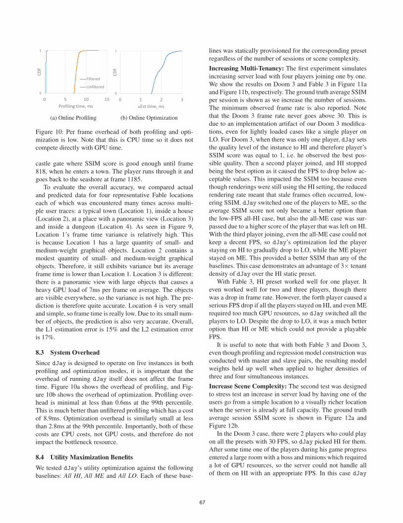
(a) Online Profiling
0
1
0 1 2 3
CDF
uEst time, ms
(b) Online Optimization
Figure 10: Per frame overhead of both profiling and opti-
mization is low. Note that this is CPU time so it does not
compete directly with GPU time.
castle gate where SSIM score is good enough until frame
818, when he enters a town. The player runs through it and
goes back to the seashore at frame 1185.
To evaluate the overall accuracy, we compared actual
and predicted data for four representative Fable locations
each of which was encountered many times across multi-
ple user traces: a typical town (Location 1), inside a house
(Location 2), at a place with a panoramic view (Location 3)
and inside a dungeon (Location 4). As seen in Figure 9,
Location 1’s frame time variance is relatively high. This
is because Location 1 has a large quantity of small- and
medium-weight graphical objects. Location 2 contains a
modest quantity of small- and medium-weight graphical
objects. Therefore, it still exhibits variance but its average
frame time is lower than Location 1. Location 3 is different:
there is a panoramic view with large objects that causes a
heavy GPU load of 7ms per frame on average. The objects
are visible everywhere, so the variance is not high. The pre-
diction is therefore quite accurate. Location 4 is very small
and simple, so frame time is really low. Due to its small num-
ber of objects, the prediction is also very accurate. Overall,
the L1 estimation error is 15% and the L2 estimation error
is 17%.
8.3 System OverheadSince dJay is designed to operate on live instances in both
profiling and optimization modes, it is important that the
overhead of running dJay itself does not affect the frame
time. Figure 10a shows the overhead of profiling, and Fig-
ure 10b shows the overhead of optimization. Profiling over-
head is minimal at less than 0.6ms at the 99th percentile.
This is much better than unfiltered profiling which has a cost
of 8.9ms. Optimization overhead is similarly small at less
than 2.8ms at the 99th percentile. Importantly, both of these
costs are CPU costs, not GPU costs, and therefore do not
impact the bottleneck resource.
8.4 Utility Maximization BenefitsWe tested dJay’s utility optimization against the following
baselines: All HI, All ME and All LO. Each of these base-
lines was statically provisioned for the corresponding preset
regardless of the number of sessions or scene complexity.
Increasing Multi-Tenancy: The first experiment simulates
increasing server load with four players joining one by one.
We show the results on Doom 3 and Fable 3 in Figure 11a
and Figure 11b, respectively. The ground truth average SSIM
per session is shown as we increase the number of sessions.
The minimum observed frame rate is also reported. Note
that the Doom 3 frame rate never goes above 30. This is
due to an implementation artifact of our Doom 3 modifica-
tions, even for lightly loaded cases like a single player on
LO. For Doom 3, when there was only one player, dJay sets
the quality level of the instance to HI and therefore player’s
SSIM score was equal to 1, i.e. he observed the best pos-
sible quality. Then a second player joined, and HI stopped
being the best option as it caused the FPS to drop below ac-
ceptable values. This impacted the SSIM too because even
though renderings were still using the HI setting, the reduced
rendering rate meant that stale frames often occurred, low-
ering SSIM. dJay switched one of the players to ME, so the
average SSIM score not only became a better option than
the low-FPS all-HI case, but also the all-ME case was sur-
passed due to a higher score of the player that was left on HI.
With the third player joining, even the all-ME case could not
keep a decent FPS, so dJay’s optimization led the player
staying on HI to gradually drop to LO, while the ME player
stayed on ME. This provided a better SSIM than any of the
baselines. This case demonstrates an advantage of 3× tenant
density of dJay over the HI static preset.
With Fable 3, HI preset worked well for one player. It
even worked well for two and three players, though there
was a drop in frame rate. However, the forth player caused a
serious FPS drop if all the players stayed on HI, and even ME
required too much GPU resources, so dJay switched all the
players to LO. Despite the drop to LO, it was a much better
option than HI or ME which could not provide a playable
FPS.
It is useful to note that with both Fable 3 and Doom 3,
even though profiling and regression model construction was
conducted with master and slave pairs, the resulting model
weights held up well when applied to higher densities of
three and four simultaneous instances.
Increase Scene Complexity: The second test was designed
to stress test an increase in server load by having one of the
users go from a simple location to a visually richer location
when the server is already at full capacity. The ground truth
average session SSIM score is shown in Figure 12a and
Figure 12b.
In the Doom 3 case, there were 2 players who could play
on all the presets with 30 FPS, so dJay picked HI for them.
After some time one of the players during his game progress
entered a large room with a boss and minions which required
a lot of GPU resources, so the server could not handle all
of them on HI with an appropriate FPS. In this case dJay
67

30 fp
s
10 fp
s
4 fp
s
30 fp
s
30 fp
s
12 fp
s30 fp
s
30 fp
s
30 fp
s
30 fp
s
30 fp
s
30 fp
s
1 player 2 players 3 players
All HI All ME All LO dJay
0
0.9
SSIM
scor
e
0.99
0.9999
0.999
(a) Doom 3
75 fp
s
40 fp
s
29 fp
s
16 fp
s
82 fp
s
78 fp
s 76 fp
s
18 fp
s83 fp
s
80 fp
s
78 fp
s
51 fp
s
75 fp
s
40 fp
s
29 fp
s
51 fp
s
1 player 2 players 3 players 4 players
All HI All ME All LO dJay
0.9999
0.9
0
0.99
0.999
SSIM
scor
e
(b) Fable 3
Figure 11: Increasing Multi-Tenancy. SSIM score of dJay is always equal to or better than baselines. dJay also maintains at
least 30 FPS whereas baselines can fall severely below acceptable FPS.
30 fp
s
10 fp
s
30 fp
s
30 fp
s
30 fp
s
30 fp
s
30 fp
s
30 fp
s
Simple scene Complex scene
All HI All ME All LO dJay
0
0.99
0.9999
SSIM
scor
e
0.9
0.999
(a) Doom 3
30 fp
s
17 fp
s
49 fp
s
20 fp
s
83 fp
s
51 fp
s
30 fp
s
40 fp
s
Simple scene Complex scene
All HI All ME All LO dJay
SSIM
scor
e
0.9999
0
0.9
0.99
0.999
(b) Fable 3
Figure 12: Increasing Scene Complexity. Again, SSIM score of dJay is always equal to or better than baselines. dJay also
maintains at least 30 FPS whereas baselines can fall severely below acceptable FPS.
dropped him to ME and left other players on HI, so that their
average SSIM score became higher than all the fixed preset
cases.
In the Fable 3 case, there were 4 players who were as-
signed the HI preset because the server’s performance was
enough for them. One of the players finished his quest inside
the house and went to the seashore where the game spawned
additional scripted animations, so that his game process re-
quired more resources than were available on the server. If
all of them kept playing on HI, they all would observe a very
low FPS and a serious SSIM score drop as shown by the HI
preset. dJay switched the GPU-heavy user to LO and left
others on HI, which was better than switching all of them
to LO. The performance tradeoff gained from one player
was enough to keep the best visual quality for the others.
This case demonstrated an advantage of 4× tenant density
of dJay over HI and ME static presets.
High Load Responsiveness: Lastly, we zoom in on dJay
under a high load situation. Figure 13 shows a case of two
Fable 3 sessions with the aggregate load spiking above the
40ms Critical level starting at frame 131. As a result, dJay
acts quickly to drop the load at frame 135. In this case,
session 1 was downgraded from HI to LO.
05
1015202530354045
0 7 14 21 28 35 42 49 56 63 70 77 84 91 98 105
112
119
126
133
140
147
Fram
e tim
e, m
s
Frame numberPlayer 1 Player 2
critical level
Figure 13: Responding quickly to high load minimizes poor
frame time.
9. Related WorkRemote rendering is a classic idea (see, e.g., [14, 21]. Yet
it was only recently that full remote execution of games on
cloud infrastructure was embraced by companies like Sony
(with their Playstation Now service), Amazon (with App-
Stream) and Nvidia (with their GRID service) as a way to
deliver high-fidelity gaming experiences on mobile devices.
A key challenge for cloud gaming products is managing the
68

infrastructure costs. Anecdotal reports about the failure of
OnLive’s game streaming service blame the cost of their in-
frastructure, because they could only support one client per
server. dJay has the potential to significantly reduce data-
center server costs by increasing the density of games exe-
cuting on a single server.
Recent research on GPU virtualization provides an im-
portant building block to enable multi-tenant game execu-
tion on cloud servers. The simplest approach, often called
pass-through, is to provide direct access to the GPU hard-
ware from a guest VM. Such solutions prevent multiple
VMs from accessing the hardware simultaneously. Early ap-
proaches to enabling 3D rendering capabilities inside a vir-
tual machine focused on virtualization at the 3D API bound-
ary: VMGL virtualizes the OpenGL v1.5 applications to run
inside guest VMs with modest overhead [19]. VMware [11]
describes their virtual GPU architectures that takes advan-
tage of GPU hardware acceleration, rather than a pure emu-
lation approach. Intel [25] describe a mediated pass-through
solution to GPU virtualization, which allows multiple guest
VMs to run a full featured GPU driver inside the guest VM,
yet also enabling multiple guest VMs to access the same
hardware.
The idea of adjusting game settings to control the load
on the GPU was introduced in Kahawai [8], although in a
very different setting. In Kahawai, the system runs a game
using low quality settings on a low-power mobile GPU and
runs the same game on a powerful GPU using high quality
settings. In contrast with dJay, these settings are static and
Kahawai does not address the problem of game server host-
ing density.
For non-GPU workloads, there is a large body of related
works. Here, we simply describe a few representative sys-
tems. Increasing multi-tenant density for non-GPU work-
loads is a widely studied problem, and recent research ef-
forts include library OSes [23] and OS containers [2, 24].
Many systems use consistent hashing for load distribu-
tion, in both data centers and wide-area distributed sys-
tems [5, 9, 16]. In big data analysis systems, SkewTune
addresses issues of data load imbalance for mapreduce com-
putations [18]. Schedulers for data center clusters have ad-
dressed fairness [15] and avoiding fragmentation and over-
allocation [12].
10. Discussion and LimitationsdJay deals with managing sessions on a single server. One
interesting avenue of further study concerns the related topic
of global admission control and session-to-server assign-
ment. Under what conditions should a client be assigned to
a server? Which server in a cluster is best suited to handling
a new client? When should a client request be rejected? In
this work, we have made the simplistic assumption that the
server can always at least meet 30 FPS at the lowest render-
ing setting for all sessions assigned to it, but clearly this de-
cision is coupled with the overall service’s session-to-server
assignment policies. The profiling and optimization tools we
have developed can lend insight into these questions higher
up in the service provider stack.
One deceptively alluring solution to providing high qual-
ity graphics to all users all the time is to simply deploy
luxury, maximum performance GPUs in the server. How-
ever, this overlooks two realities. First, the best price-for-
performance GPUs are midrange. Luxury GPUs are expen-
sive and therefore not a realistic option for service providers.
Second, rendering demands have increased commensurate
with GPU performance boosts for the past two decades. We
cannot simply wait for Moore’s law to provide free cycles
because new rendering algorithms offering even better vi-
sual effects will likely be ready to use the new capacity.
Thus far we have used only a handful of rendering setting
presets. For even more granular video quality control, it is
also interesting to consider the space of all possible render-
ing settings. For example, Fable 3 presents at least eight di-
mensions for manipulating rendering settings (Table 2b). As
dJay delves into more settings options, it needs commen-
surately more profiling trace data in order to build a model
that accurately predicts each setting. While the exact data
volume needed is an open question, we have shown that it
is low overhead to collect more data online from active ses-
sions.
While we have shown dJay working with two production
games, future work includes extending dJay to a broader
class of games, such as multiplayer and 2D. In a multi-
player setting, the GPU load induced by other players are
still manifested as changes in the set of visible game objects.
Therefore, dJay should still compute utilities appropriately.
During profiling of a multiplayer game, updates from other
players would need to be vectored to both master and slave.
In addition, further game modifications would be needed in
order to have only master (or only slave) send updates to
other players. 2D games should be straightforward to sup-
port. Rather than modifying each game individually, it is ap-
pealing to consider implementing dJay as a game engine
modification. Game engines such as Unity and Unreal al-
ready power the vast majority of games. The key dJay mod-
ifications (deterministic execution, exposure of AOL/POL
and rendering setting changes) appear feasible at the game
engine level.
11. ConclusionFrom the perspective of a cloud gaming service provider,
dJay lowers costs by achieving up to 4× better multi-tenant
density over existing approaches. It takes advantage of the
observation that dynamically changing rendering settings
can help to achieve frame rate targets when under load.
Moreover, by formulating the rendering settings assign-
ment problem as utility-optimizing Multiple Choice Knap-
sack Problem, dJay provides optimal visual quality when
resources are available.
69

References[1] Amazon appstream. http://aws.amazon.com/
appstream.
[2] Lxc. http://linuxcontainers.org.
[3] Nvidia grid cloud gaming. http://shield.nvidia.com/
grid.
[4] Sony playstation now streaming. http://us.
playstation.com/playstationnow.
[5] A. Adya, J. Dunagan, and A. Wolman. Centrifuge: Integrated
lease management and partitioning for cloud services. In
NSDI, 2010.
[6] M. Armbrust, A. Fox, R. Griffith, A. D. Joseph, R. Katz,
A. Konwinski, G. Lee, D. Patterson, A. Rabkin, I. Stoica, and
M. Zaharia. A view of cloud computing. Commun. ACM,
53(4):50–58, Apr. 2010.
[7] M. Claypool, K. Claypool, and F. Damaa. The effects of
frame rate and resolution on users playing first person shooter
games, 2006.
[8] E. Cuervo, A. Wolman, L. P. Cox, K. Lebeck, A. Razeen,
S. Saroiu, and M. Musuvathi. Kahawai: High-quality mobile
gaming using gpu offload. In MobiSys, May 2015.
[9] G. DeCandia, D. Hastorun, M. Jampani, G. Kakulapati,
A. Lakshman, A. Pilchin, S. Sivasubramanian, P. Vosshall,
and W. Vogels. Dynamo: Amazon’s highly available key-
value store. In SOSP, 2007.
[10] M. Deloura. Game Programming Gems. Charles River Media,
Inc., Rockland, MA, USA, 2000.
[11] M. Dowty and J. Sugerman. Gpu virtualization on vmware’s
hosted i/o architecture. In WIOV, 2008.
[12] R. Grandl, G. Ananthanarayanan, S. Kandula, S. Rao, and
A. Akella. Multi-resource packing for cluster schedulers. In
SIGCOMM, 2014.
[13] S. Hollister. Onlive lost: how the paradise of streaming games
was undone by one man’s ego. http://www.theverge.
com/2012/8/28/3274739/onlive-report, 2012.
[14] G. Humphreys, M. Houston, R. Ng, R. Frank, S. Ahern,
P. D. Kirchner, and J. T. Klosowski. Chromium: A stream-
processing framework for interactive rendering on clusters.
In Proceedings of the 29th Annual Conference on Computer
Graphics and Interactive Techniques, SIGGRAPH ’02, pages
693–702, New York, NY, USA, 2002. ACM.
[15] M. Isard, V. Prabhakaran, J. Currey, U. Wieder, K. Talwar,
and A. Goldberg. Quincy: Fair scheduling for distributed
computing clusters. In SOSP, 2009.
[16] D. Karger, A. Sherman, A. Berkheimer, B. Bogstad, R. Dhani-
dina, K. Iwamoto, B. Kim, L. Matkins, and Y. Yerushalmi.
Web caching with consistent hashing. In WWW, 1999.
[17] H. Kellerer, U. Pferschy, and D. Pisinger. Knapsack Problems.
Springer Science and Business Media, 2004.
[18] Y. Kwon, M. Balazinska, B. Howe, and J. Rolia. Skewtune:
Mitigating skew in mapreduce applications. In SIGMOD,
2012.
[19] H. A. Lagar-Cavilla, N. Tolia, M. Satyanarayanan, and
E. de Lara. Vmm-independent graphics acceleration. In VEE,2007.
[20] K. Lee, D. Chu, E. Cuervo, J. Kopf, Y. Degtyarev, S. Grizan,
A. Wolman, and J. Flinn. Outatime: Using speculation to
enable low-latency continuous interaction for cloud gaming.
MobiSys 2015, May 2015.
[21] W. R. Mark, L. McMillan, and G. Bishop. Post-rendering 3d
warping. In Proceedings of the 1997 Symposium on Interac-tive 3D Graphics, I3D ’97, pages 7–ff., New York, NY, USA,
1997. ACM.
[22] S. Martello and P. Toth. Knapsack Problems: Algorithms andComputer Implementations. John Wiley & Sons, Inc., New
York, NY, USA, 1990.
[23] D. E. Porter, S. Boyd-Wickizer, J. Howell, R. Olinsky, and
G. Hunt. Rethinking the library os from the top down. In
ASPLOS, 2011.
[24] D. Price and A. Tucker. Solaris Zones: Operating System
Support for Consolidating Commercial Workloads. In LISA,
2004.
[25] K. Tian, Y. Dong, and D. Cowperthwaite. A full gpu virtual-
ization solution with mediated pass-through. In USENIX ATC,
2014.
[26] Z. Wang, A. C. Bovik, H. R. Sheikh, and E. P. Simoncelli.
Image quality assessment: From error visibility to structural
similarity. Trans. Img. Proc., 13(4):600–612, Apr. 2004.
70


![Thema heute: Lokalisierung - KIT - ITI Algorithmik I · HS ist 1-kompetitiv in einer Dimension. [O’Dell, Wattenhofer, 2005]. [O’Dell, Wattenhofer, 2005]. Man kann zeigen, dass](https://img.pdfslide.net/doc/110x75/5d4ef72088c99367198be6f2/thema-heute-lokalisierung-kit-iti-algorithmik-i-hs-ist-1-kompetitiv-in.jpg)