Cooling a Solar Telescope Enclosure: Plate Coil Thermal Analysis

Michael GormanSyracuse University

Mentor: Chriselle GalaponCo-Mentors: Guillermo Montijo Jr., LeEllen Phelps

Daniel K. Inouye Solar Telescope (DKIST)

Reference Material

16124-TRE-046-2-Carousel Cooling System Analysis Report

Abstract

The climate of Haleakalā requires the observatories to actively adapt to changing conditions in order to produce the best possible images. Observatories need to be maintained at a temperature closely matching ambient or the images become blurred and unusable. The Daniel K. Inouye Solar Telescope is a unique telescope as it will be active during the day as opposed to the other night-time stellar observatories. This means that it will not only need to constantly match the ever-changing temperature during the day, but also during the night so as not to sub-cool and affect the view field of other telescopes while they are in use.

To accomplish this task, plate coil panels will be installed on the DKIST enclosure that are designed to keep the temperature 2˚ Celsius below ambient temperature. To ensure this, a test rig has been installed at the summit of Haleakalā. The project’s purpose is to verify that the plate coil panels are capable of maintaining this temperature throughout all seasons and involved collecting data sets of various variables including pressures, temperatures, flows of coolant, solar radiations and wind velocities during typical operating hours. Using MATLAB, a script was written to observe the plate coil’s thermal performance. The plate coil did not perform as expected, achieving a surface temperature that was generally 2ºC above ambient temperature. This isn’t to say that the plate coil does not work, but the coolant pumped through the plate coil may not be set to a low enough temperature. Calculated heat depositions were about 23% lower than that used as the basis of the of the design, a reasonable agreement given the fact that many simplifying assumptions done in the model. These were not carried over into the testing.

It is recommended to do additional testing at different angles of attack and pressures. This would allow a more full analysis. It’s also recommended to use a larger chiller for the plate coil or to set the coolant flowing through the plate coil to a lower temperature.

1. Introduction

The carousel cooling system is designed to keep the DKIST at a temperature close to that of ambient. Keeping the enclosure at this temperature helps minimize dome-seeing effects,

turbulent fluctuations of the index of refraction due to differential temperatures within the air along the light path cause by the sun heating the enclosure surface..

The plate coils needs to be able to reject heat so as to not radiate any stored heat during the night. Pan-STARRS 1 and 2 as well as the Faulkes North telescope are located closely to the DKIST facility; any heat radiated off of the observatory during the night would likely impact data taken by these telescopes during the night.

The entire carousel cooling system is separated into 64 zones of plate coils that are installed on top of a cladding surface. These 64 zones each have one pair of supply and return coolant lines. The plate coils in these zones are connected in a few parallel circuits of a few piece of plate coil in series, the number of which depending on the location and shape of that particular zone. Dynalene HC-20 is filled, pressurized and fed into the plate coil systems at a temperature 4˚ Celsius below ambient temperature and allowed to exit the zone as it approaches ambient temperature.

The basic principal behind running these tests is to authenticate the design assumptions. The test rig is the same shape and average size (5’ x 8’) as the vast majority of the panels put on the enclosure. The design data is based off of numbers recorded on July 1st, 2003. The first run of test rig data was recorded on July 1st, 2015, with an additional test being run on July 15th, 2015. Other tests had been done in the past three seasons.

In order to calculate the required values quickly, a MatLAB script was constructed that calculates heat depositions, heat loads, performs graphical models, and explains if the test rig meets standards. The script has been designed in order to input past and future data smoothly through use of excel spreadsheets.

2. Test Rig Configuration

The test rig is, as explained, a 5’ x 8’ rectangle. This is the most common size that will be installed on the enclosure surface. Twenty-four surface bolts hold the test rig together, in columns of 4 and rows of 6. (As seen in Figure 1).

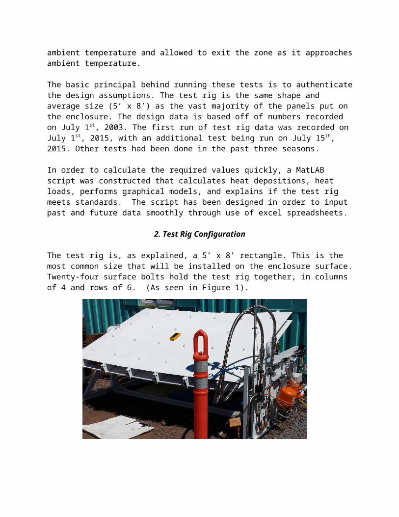
(Figure 1: The Test Rig Configuration)

The test rig is connected to a base that allows the plate coil to rotate to various different angles of attack. Ranging from 90˚ to 0˚ (not exact but close to these). The plate coil can be locked at these angles, so it is possible to take measurements that would be similar to different zones on the enclosure. This is also useful in seeing how the plate coil performs in direct sunlight and in partial sunlight.

The Dynalene HC-20 is pumped into the plate coil through an external system. The pump system is designed to cool one side or the other of the plate coil, however it is uncommon that both sides will ever be cooled. A chiller is used to cool the Dynalene to a temperature 4˚ C below ambient (This may need to be dropped lower depending on how well the chiller is operating). This chilled Dynalene is pumped into the system and then returned back into the chiller.

The pump system is designed with a chiller, booster pump and Venturi Pump. The booster is used to increase the pressure and flow and the Venturi Pump is used to relieve strain on the system. The booster pump does not need to be turned on at all times. However for some tests, it is required to develop sufficient system pressure and flow.

Two valves are also positioned in the systems to control the flow. These can be opened proportionally from 0% to 100%. For the purposes of these tests the proportional control values were set at 0, 50, and 100%.

The rig is set up within 150 feet of the actual telescope. Test rig altitude is around 3,050 m, latitude 20.71 N and longitude 156.25 W. The plate coil can’t be observed at its peak height of 43.6 m.

It’s important to note, that the test rig had been set up reversed as compared to the design. The supply and return tubes had been mixed up. Tests were run in both ways in order to see if this merited a large change in data or not.

3. Test ProcedureTest PreparationBefore the plate coil pump system is plugged in, the following needs to be accomplished and checked:

The plate coil is unwrapped and released from all securing mechanisms The pump system is checked for any leaks or residue.

o IMPORTANT: While not considered toxic, Dynalene still cannot be spilled at the test site.

o If there are any leak or residue, clean with a wet rag and make sure that those valves and pipes are securely fitted.

Depending on the amount of time that has passed in between test sessions, the plate coil may need to be “burped”.

Ensure that the plate coil is set to its prescribed angle of attack for the test. Make sure that all instruments are installed and are ready to record data Chiller should to be set 4ºC below ambient temperature (Might need to be set

colder) Before data is recorded, allow the plate coil to stabilize at test pressure.

Procedure

Varied control and isolation valve setups are achieved to set different flow characteristics along with corresponding vertical and horizontal positioning of the test rig plate coil. This is done to ensure that the plate coil is seeing different sun radiation and heat input angles. This also allows the data to better correspond with the results achieved in TRE-046.

Testing included different angles of attack, variable pressure through operation of the booster pump-throttling valve, stroking of control vales, setting isolation vales and swapping the plate coil supply and return hoses. All of these were performed, for the purpose of performance comparison with previous tests and the model.

Test data should be recorded onto an excel sheet (PC_Data_Sheet). Date and time is recorded with each plate coil test. Spreadsheet data is then input to the MATLAB program, and then run through the MATLAB script.

Test Equipment Swagelok miniature industrial pressure gages Dynasonics DNX portable ultrasonic flow meter Fluke 754 Process Calibrator with surface temperature probes Seaward SS200R solar irradiance meter Windmate WM-300 handheld weather station Omega surface mount thermistor sensors FLIR T620bx Thermal Imaging Camera

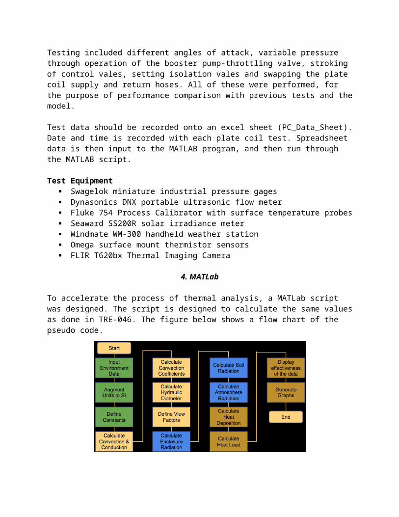
4. MATLab

To accelerate the process of thermal analysis, a MATLab script was designed. The script is designed to calculate the same values as done in TRE-046. The figure below shows a flow chart of the pseudo code.

(Figure 2: MATLab Pseduo code)

The data sets captured on July 1st and 15th were input to excel sheets. The older tests were also captured electronic. It’s recommended that all future data be re-recorded unto the blank excel file.

The code calculates many parameters including heat depositions and heat loads, the primary points of interest. In addition to these, average ambient temperatures, skin temperatures and percentage errors are taken into consideration. Graphs are created based on solar radiation vs. Heat Depositions, Time of day vs. Heat Deposition and Time of Day vs. Heat load. Finally, there are two display outputs that display whether the plate coil is performing to standard, and if the data was recorded at an optimal time of day.

5. Results

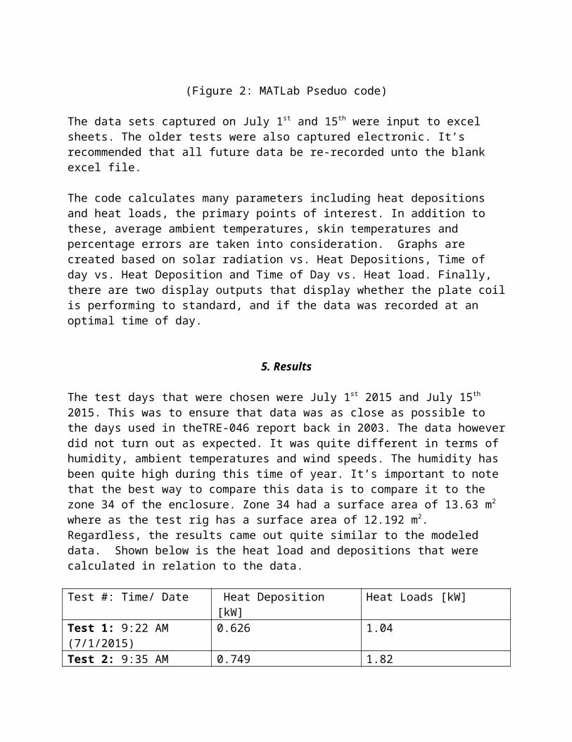
The test days that were chosen were July 1st 2015 and July 15th 2015. This was to ensure that data was as close as possible to the days used in theTRE-046 report back in 2003. The data however did not turn out as expected. It was quite different in terms of humidity, ambient temperatures and wind speeds. The humidity has been quite high during this time of year. It’s important to note that the best way to compare this data is to compare it to the zone 34 of the enclosure. Zone 34 had a surface area of 13.63 m2 where as the test rig has a surface area of 12.192 m2. Regardless, the results came out quite similar to the modeled data. Shown below is the heat load and depositions that were calculated in relation to the data.

Test #: Time/ Date Heat Deposition [kW] Heat Loads [kW]Test 1: 9:22 AM (7/1/2015)

0.626 1.04

Test 2: 9:35 AM (7/1/2015)

0.749 1.82

Test 3: 9:45 AM (7/1/2015)

0.786 1.91

Test 4: 9:50 AM (7/1/2015)

0.649 1.75

Test 5: 9:59 AM (7/1/2015)

0.671 2.33

Test 6: 10:09 AM (7/1/2015)

0.831 2.44

Test 7: 10:17 AM (7/1/2015)

0.854 2.65

Test 8: 10:23 AM (7/1/2015)

0.803 2.65

Test 9: 9:30 AM (7/15/2015)

0.636 0.961

Test 10: 9:50 AM (7/15/2015)

0.793 1.03

Test 11: 10:00 AM (7/15/2015)

0.827 1.42

Test 12: 10:09 AM (7/15/2015)

0.698 1.59

Test 13: 10:14 AM (7/15/2015)

0.740 2.17

Test 14: 10:21 AM (7/15/2015)

0.880 2.39

Test 15: 10:30 AM (7/15/2015)

0.894 1.24

Test 16: 10:35 AM (7/15/2015)

0.749 1.27

Looking at the times in which the data was recorded, they were recorded within the 9:00 and 10:00 hours. These are the best times in order to get the most useful data. The modeled data predicted that at Zone 34, during the 9:00 hour, the deposition would be at 1.24 kW. It also predicts that during the 10:00 hour the same zone will have a deposition of 0.80 kW. Taking the average of these gives and average heat deposition of 1.02 kW. The overall percentage error was calculated to 23.32%. This can be attributed to the simplifications that were made during the modeling process. Blackbodies were assumed and certain radiations were all together left out. This will merit changes in the calculation process.

The data sets from previous seasons have also been analyzed. Nothing was obscure when it came to previous data sets. The percentage error over all the previous data sets together came to 23.53%. Below are three graphs that compare every test that’s been taken over the past two years.

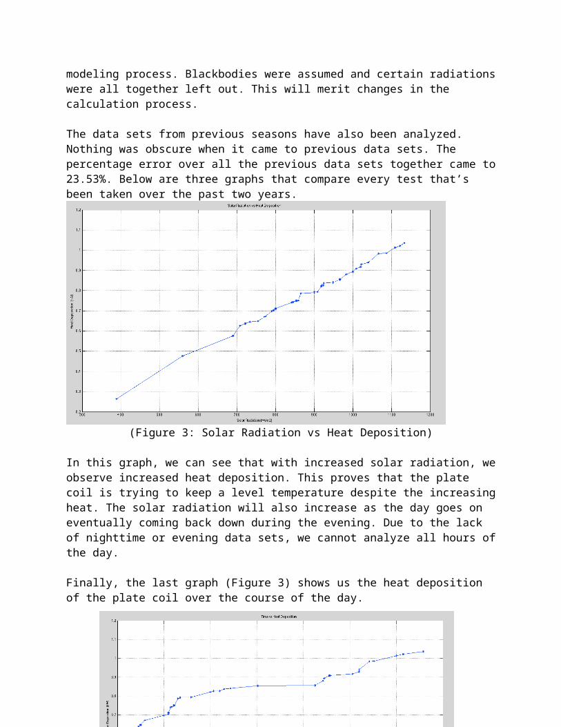
(Figure 3: Solar Radiation vs Heat Deposition)

In this graph, we can see that with increased solar radiation, we observe increased heat deposition. This proves that the plate coil is trying to keep a level temperature despite the increasing heat. The solar radiation will also increase as the day goes on eventually coming back down during the evening. Due to the lack of nighttime or evening data sets, we cannot analyze all hours of the day.

Finally, the last graph (Figure 3) shows us the heat deposition of the plate coil over the course of the day.

(Figure 4: Heat Deposition vs Time of Day)

What’s interesting to note here is the plateau of the heat deposition towards the middle of the day. The solar radiation tends to stay around the same, around 1000 W/m2. If more data were to be recorded, spanning the entire 24-hour period, we’d see a sudden drop off towards the end.

The flow for flow meter 2, has been acting up and been giving faulty data. Recommend a new flow meter, or a change to the amount of bounces or bounce path. The values for flow 2 have been taken as is. The pressure gage for pressures 4 and 5 both had issues with leakages. These were taken out and plugged. Therefore, none of the tests recorded in July will have these pressures.

Further more, this data recording method is somewhat inefficient if done with a single person. Recommend developing a method to quickly record large sets of data over time periods. This will be difficult knowing that all the recording methods are different (some by hand, some by computer). It’s also important to note about the time frame, panels are to be installed within the next year and it might not be feasible to spend the time developing a more efficient recording method.

The thermal imaging was done on July 15th 2015 as well. A 7-minute video was done after letting the plate coil settle to a uniform temperature. The flow was set up as the design intended. The flow was observed to flow relatively well. Due a small difference in pressures, the top of the plate coil seemed to cool faster than the bottom. The figure below shows an image of the thermal analysis.

(Bottom of this Page Left Blank)

(Figure 5: Thermal Imaging)

What are important to see in the above image are the temperatures of the plate coil across all of the different spots. The surface stays a pretty steady uniform temperature. However, the ambient temperature during this time was, at its highest 14.5 ºC. This is unfortunate to see as the plate coil is not below its 2-degree threshold.

Finally, the tests that were run on the 1st and 15th of July were set up to design standards. (ie. The hoses in the correct spots). There were no substantial differences between these tests and tests down in the past. So it’s safe to assume that the hose position does not affect the effectiveness of the plate coil.

6. Conclusion

The plate coil seems to be performing to design specs. The 23% error can be attributed to the fact that the values used during the modeled process are not the same as the recorded data. This includes: Solar Radiations, Humidity, Ambient and Soil temperatures, and wind velocities. The modeled data, going off of the July 1st, 2003 data, generally had higher temperatures and radiations. We can also note that the modeled data assumed a lot of values. Simplifying assumptions such as blackbodies and neglecting certain radiations will change the final values. This would help explain the disparity between the model and test rig performance. A buffer zone of 2 degrees above ambient was allowed, but this is not what was modeled. However, going strictly off of the modeled data, the plate coil is not performing its job.

Recommend improving the pump setup a bit, the miss-match of metal types used for the piping system should be unified (recommend copper). The plate coil has the ability to cool one side or the other, I feel this is overly designed if we only plan on having one side cooled. Finally, due to the fact that the plate coil was not below ambient temperature, it’s recommended that a larger chiller be installed or the temperature set point of the chiller be turned down tow 10ºC below ambient.

Finally, it would also be interesting to get data from all hours of the day (including at night). Its understood that that the data was recorded during the most intense parts of the day, but it would give a more full result section and give the graphs more data to work with.

ACKNOWLEDGEMENT

The DKIST is managed by the National Solar Observatory (NSO), which is operated by the Association of Universities for Research in Astronomy, Inc. (AURA) under a cooperative agreement with the National Science Foundation (NSF).

The 2015 Akamai Internship Program is part of the Akamai Workforce Initiative, in partnership with the Univ. of California, Santa Cruz; the Univ. of Hawai'i Institute for Astronomy; and the Thirty Meter Telescope (TMT) International Observatory.  Funding is provided by the Air Force Office of Scientific Research (FA9550-10-1-0044); Univ. of Hawai'i; and TMT International Observatory."