Forschungsinstitut zur Zukunft der ArbeitInstitute for the Study of Labor

DI

SC

US

SI

ON

P

AP

ER

S

ER

IE

S

Do Higher Corporate Taxes Reduce Wages?

IZA DP No. 9606

December 2015

Clemens FuestAndreas PeichlSebastian Siegloch

Do Higher Corporate Taxes

Reduce Wages?

Clemens Fuest ZEW, University of Mannheim, CESifo and IZA

Andreas Peichl

ZEW, University of Mannheim, IZA and CESifo

Sebastian Siegloch

University of Mannheim, IZA, ZEW and CESifo

Discussion Paper No. 9606 December 2015

IZA

P.O. Box 7240 53072 Bonn

Germany

Phone: +49-228-3894-0 Fax: +49-228-3894-180

E-mail: iza@iza.org

Any opinions expressed here are those of the author(s) and not those of IZA. Research published in this series may include views on policy, but the institute itself takes no institutional policy positions. The IZA research network is committed to the IZA Guiding Principles of Research Integrity. The Institute for the Study of Labor (IZA) in Bonn is a local and virtual international research center and a place of communication between science, politics and business. IZA is an independent nonprofit organization supported by Deutsche Post Foundation. The center is associated with the University of Bonn and offers a stimulating research environment through its international network, workshops and conferences, data service, project support, research visits and doctoral program. IZA engages in (i) original and internationally competitive research in all fields of labor economics, (ii) development of policy concepts, and (iii) dissemination of research results and concepts to the interested public. IZA Discussion Papers often represent preliminary work and are circulated to encourage discussion. Citation of such a paper should account for its provisional character. A revised version may be available directly from the author.

IZA Discussion Paper No. 9606 December 2015

ABSTRACT

Do Higher Corporate Taxes Reduce Wages?* This paper estimates the incidence of corporate taxes on wages using a 20-year panel of German municipalities. Administrative linked employer-employee data allows estimating heterogeneous worker and firm effects. We set up a general theoretical framework showing that corporate taxes can have a negative effect on wages in various labor market models. Using an event study design, we test the predictions of the theory. Our results indicate that workers bear about 40% of the total tax burden. Empirically, we confirm the importance of both labor market institutions and profit shifting possibilities for the incidence of corporate taxes on wages. JEL Classification: H2, H7, J3 Keywords: business tax, wage incidence, administrative data, local taxation Corresponding author: Andreas Peichl Centre for European Economic Research (ZEW) L7,1 68161 Mannheim Germany E-mail: peichl@zew.de

* We would like to thank Hilary Hoynes, the editor, and three anonymous referees for their helpful comments. We are indebted to W. Arulampalam, A. Auerbach, R. Blundell, D. Card, R. Chetty, M. Devereux, P. Doerrenberg, D. Duncan, G. Friebel, J. Hines, H. Kleven, G. Maffini, A. Oswald, M. Overesch, T. Piketty, E. Saez, J.C. Suarez Serrato, J. Voget, D. Yagan, O. Zidar, as well as numerous conference and seminar participants for valuable comments and suggestions on earlier versions (sometimes circulating as “Do Employees Bear the Burden of Corporate Taxation? A Micro Level Approach Using Linked Employer-Employee Data”).

1 Introduction

Most economists think that labor bears part of the burden of corporate taxation.1 How-

ever, there is considerable disagreement on how much of the corporate tax burden is

shifted onto workers. The theoretical literature, inspired by Harberger (1962)’s seminal

contribution, predicts that the incidence on wages depends on the assumptions regarding

the openness of the economy (Diamond and Mirrlees, 1971; Bradford, 1978; Kotlikoff and

Summers, 1987; Harberger, 1995), its sectoral composition (Shoven, 1976), savings be-

havior (Feldstein, 1974; Bradford, 1978) and the presence of uncertainty in the economy

(Ratti and Shome, 1977).2 Little attention has been paid to the role of wage setting

institutions and labor market frictions. With the exception of Felix and Hines (2009) and

Arulampalam et al. (2012) who study corporate taxes in a wage bargaining context, most

existing studies assume a competitive labor market.

Credible empirical evidence on the incidence of corporate taxes is scarce. Sufficient

and exogenous variation in corporate tax rates is essential for identifying the causal effect

of higher corporate taxes. Cross-country research designs (such as Hassett and Mathur,

2006; Felix, 2007; Desai et al., 2007) must defend their (implicit or explicit) common

trend assumptions. Single-country designs can establish a valid control group more easily.

Most existing studies (such as Dwenger et al., 2011; Arulampalam et al., 2012; Liu

and Altshuler, 2013), however, have to rely on variation in the tax burden that is not

driven solely by policy reforms but also by firm choices. For instance, differences in tax

burdens across industries or due to formula apportionment may depend directly on sales

and investment activities which might be endogenous to tax rates as well. In a recent

contribution, Suarez Serrato and Zidar (2014) calibrate a spatial equilibrium model based

on reduced-form estimates exploiting changes in tax rate differentials and variation from

formula apportionment weights across the 52 U.S. federal states.3

In this paper, we revisit the question of the incidence of corporate taxes on wages

both theoretically and empirically. First, we develop a theoretical model that explicitly

accounts for the role of wage setting institutions and labor market frictions for the inci-

dence of corporate taxation. Second, we exploit the specific institutional setting of the

German local business tax (LBT)4 to identify the corporate tax incidence on wages.

1 For example, public economists surveyed by Fuchs et al. (1998) respond on average that 40% of thecorporate tax incidence is on capital (with an interquartile range of 20–65%) leaving a substantial shareof the burden for labor (and land owners or consumers).

2 Surveys of the literature are provided by Auerbach (2005) and Harberger (2006). Computationalgeneral equilibrium (CGE) models find that labor bears a substantial share of the corporate tax burdenunder reasonable assumptions (see Gravelle, 2013, for an overview).

3 Felix and Hines (2009) also use U.S. state variation but rely on cross-sectional data.4 See, e.g., Buttner (2003); Janeba and Osterloh (2012); Foremny and Riedel (2014) for studies ana-

1

In the first part of the paper, we set up a general theoretical framework that allows

us to derive testable predictions for the effect of corporate tax changes on wages under

different assumptions regarding wage setting institutions and labor market frictions. In

most settings, higher corporate taxes reduce wages, albeit for different reasons. This

holds true in particular for models with individual and collective wage bargaining, fair

wage models, models where higher wages allow firms to hire more productive workers and

monopsonistic labor markets. However, the wage effects are diluted and may disappear

completely if collective bargaining takes place at the sector-level (compared with the firm-

level), if there is formula apportionment for firms operating in multiple jurisdictions or if

firms react to higher corporate taxes by shifting income to the personal income tax base

or to other countries.

In the second part, we test the theoretical predictions using administrative panel

data on German municipalities from 1993 to 2012. Germany is well suited to test our

theoretical model for several reasons. First, we have substantial tax variation at the local

level. From 1993 to 2012, on average 12.4% of municipalities adjusted their LBT rates per

year. Eventually, we exploit 17,999 tax changes in 10,001 municipalities between 1993 to

2012 for identification.5 Compared to cross-country studies, the necessary common trend

assumption is more likely to hold in our setting since municipalities are more comparable

than countries. Second, municipalities can only change the LBT rate, while the tax base

definition and liability conditions are determined at the federal level.6 Hence, the variation

in tax rates we exploit empirically does not depend on (current) firm choices. Moreover,

the municipal autonomy in setting tax rates allows us to treat municipalities as many small

open economies within the highly integrated German national economy – with substantial

mobility of capital, labor and goods across municipal borders. General equilibrium effects

on interest rates or consumer prices are therefore likely to be of minor importance in this

setting. This is likely to be true even for sectors producing non-tradeable goods like the

service sector since individuals may buy these services in the neighboring municipality.

Third, the German labor market is characterized by a variety of wage setting institutions

which include sector and firm-level collective bargaining as well as wage setting on the

basis of contracts between firms and individual employees. In order to shed light on the

specific interactions of labor market institutions and tax changes, we match the municipal

lyzing the LBT.5 Bauer et al. (2012) also investigate the LBT. However, as in an earlier version of this paper (Fuest

et al., 2011), they average tax rates on the county level (consisting of 28 municipalities on average). Dueto this aggregation, firms in unaffected municipalities are wrongly exposed to a change in the county’saverage tax rate leading to biased results. Moreover, Bauer et al. (2012) lack relevant firm data becausethey do not use linked employer-employee data.

6 Kawano and Slemrod (2012) compare a large number of reforms of nationwide corporate taxes andshow that tax rate change are usually combined with changes in the tax base as well.

2

data to administrative linked employer-employee micro data that combine social security

records with a representative firm survey.

We apply an event study design to estimate the effect of corporate tax changes on

wages and test the predictions of our theoretical model.7 We find a negative overall effect

of higher corporate taxes on wages. For a 1-euro increase in the tax bill, the wage bill

decreases by 56 cents.8 Assuming a marginal excess burden of the corporate tax of 29%

(Devereux et al., 2014), about 43% of the incidence of the local business tax is borne by

workers. Our findings are robust to the inclusion of a comprehensive set of very local

and flexible controls (including “commuting-zone × year” fixed effects) suggesting that

omitted variables such as local shocks are not driving our results. Moreover, we find no

effects for firms that are exempt from the LBT.

In the next step, we test for heterogeneous tax effects on the firm and worker level.

We find more pronounced negative effects in firms with firm-level compared to sector-level

bargaining agreements. For firms that are not covered by bargaining agreements, we also

find negative wage effects. Among firms not covered by the bargaining agreements, firms

that take sectoral collective bargaining agreements as a reference point show stronger

responses. One interpretation of this finding is that fair wage considerations may play

a role in these cases. Looking at single-plant versus multi-plant firms, we find negative

wage effects only for the former, which is in line with the theoretical prediction that wage

effects will be smaller in multi-establishment firms because they are subject to formula

apportionment and may be able to shift profits regionally or internationally. In terms of

worker heterogeneity, we find that female workers are affected more strongly. This finding

could be rationalized with a monopsonistic labor market model and relatively more elastic

labor supply for these groups.

We contribute to the literature in several ways. First, we provide new estimates for

the corporate tax incidence on wages exploiting the German institutional setting, which

gives rise to substantial variation in tax rates. Second, going beyond the German case,

our general theoretical analysis highlights the role of labor market institutions for tax

incidence, which has not received much attention so far. The relevance of the different

types of labor market frictions that we consider differs across countries. While unions are

strong in some countries, others exhibit more competitive labor markets where individual

wage bargaining might be more relevant, as assumed in search and matching models.9 In

7 The event study design also allows to check for reverse causality. These checks do not suggest thatreverse causality drives our results.

8 Note that only very few nominal wage decreases are observable in the data. Our wage responses arerather driven by lower nominal wage increases leading to lower nominal wage levels in the future in thetreated municipalities.

9 Unions are especially important in Northern and Continental European countries, as well as Aus-

3

addition, fair wage considerations or firms that set higher wages to hire more productive

workers are also likely to be relevant in many countries. Third, our detailed linked-

employer employee data allows us to investigate heterogeneous firm and worker effects and

test many of our theoretical predictions. For instance, we observe firms with and without

collective bargaining agreements, which allows us to empirically test the role of different

labor market frictions predicted by the theory. Furthermore, we find differences in tax

incidence between small versus large firms and profitable versus less profitable firms, which

are likely to be important in other countries as well. Last, we study corporate taxation

at the subnational level which is important in many countries.10 Compared to changes

in state or national corporate tax rates, two potential differences are worth noting. On

the one hand, relative mobility of labor might be lower at a more aggregated level, which

should lead to larger wage effects of tax changes. On the other hand, price effects are

likely to be more important when looking at state or national tax changes, which should

decrease the incidence on labor.

The rest of the paper is structured as follows. In Section 2, we discuss the incidence

of corporate taxes on wages in a broad theoretical framework, paying special attention

to the interaction of labor market institutions and corporate taxation. In Section 3, we

briefly describe the German institutional setting, in particular the corporate tax system

focusing on the LBT, whose variation we exploit in the empirical part of the paper.

The empirical model is set up in Section 4.1. Section 4.2 presents the administrative

linked employer-employee dataset used for the analysis. Empirical results are shown and

discussed in Section 5. Section 6 presents our conclusions.

2 The theory of corporate tax incidence

The theoretical literature has produced a variety of models on corporate tax incidence.

These models lead to different predictions, depending on the assumptions made about

factor and output markets, wage setting institutions, the structure of the tax system

and behavioral reactions to tax changes. In the seminal paper by Harberger (1962),

the economy is closed, labor markets are competitive and capital is in fixed supply.11

The corporate tax is a tax per unit of capital, which distorts investment between the

incorporated and the unincorporated sector. At least for plausible parameter values, the

tralia, Canada, New Zealand and Mexico – see the OECD Trade Union Density statistics: http:

//stats.oecd.org/Index.aspx?DataSetCode=UN_DEN.10 For OECD countries, prominent examples include the U.S., Canada, France, Italy, Japan, Spain and

Switzerland (see, e.g., Bird, 2003; Spengel et al., 2014, for overviews).11 Feldstein (1974) and Ballentine (1978) study the tax incidence in models with endogenous savings

and find that part of the tax burden is shifted to labor.

4

tax burden is almost fully borne by capital.

While the closed economy assumption is a key feature of the Harberger model, the

more recent literature has emphasized international capital mobility (see e.g. Bradford,

1978; Kotlikoff and Summers, 1987; Harberger, 2006). In open economies, the share of

the corporate tax burden borne by domestic immobile factors increases as the economy

relative to the rest of the world decreases.12 In the case of a small open economy that

faces a perfectly elastic supply of capital, the burden of the corporate tax is fully borne

by factors other than capital.13 If profits of a firm are the result of location specific rents,

the tax will partly fall on these rents. By contrast, if rents are firm specific and firms

are mobile, the tax burden will be fully shifted to owners of immobile factors like land or

labor (see Kotlikoff and Summers, 1987, section 3).14

In a setting with local corporate taxes and with both labor and capital mobility

across jurisdictions, a decline in wages in response to higher taxes would induce workers

to seek employment in other jurisdictions. In the case of perfect labor mobility and com-

petitive labor markets, the wage rates would be determined in the national labor market

and individual local corporate tax changes would not affect the wage rate. Assuming that

output prices are little affected by changes in local tax rates, higher local corporate taxes

would fall on land or reduce other location-specific rents.

The assumption that mobility makes wages completely independent of local condi-

tions is restrictive, however, and not just because of mobility costs. One reason why this

assumption may not hold is that local public services may affect migration decisions. If

a corporate tax change leads to higher local public spending, workers might accept lower

wages in return for better public services. Thus, higher corporate taxes may lead to lower

local wages if accompanied by more public services. This would suggest that higher local

taxes reduce wages even in tax exempt firms.

Another restrictive assumption is that labor markets are competitive. To understand

the impact of corporate tax changes on wages it is important to take into account labor

market imperfections and wage setting institutions. In the next subsections, we develop

a simple theoretical framework that enables the study of corporate tax incidence in the

presence of various forms of labor market imperfections.

12 This applies to a source based corporate income tax. Residence based taxes may have more compli-cated incidence effects. Most existing corporate taxes are, in effect, source based taxes.

13 From a global perspective, a tax increase in one jurisdiction reduces the income of immobile laborin that jurisdiction but increases labor income and reduces capital income in the rest of the world. Thispoint was first made by Bradford (1978), with respect to prices of immobile property.

14 In principle, the tax burden may also fall on suppliers or on customers, provided input and outputprices are not pinned down by international markets.

5

2.1 A model of corporate tax incidence with labor market im-perfections

Labor market theory has produced many ideas and views about how wages and employ-

ment are determined. In the following, we discuss the implications of various labor market

models for corporate tax incidence. As a benchmark, we start with the case of competitive

labor markets. We then turn to models with wage bargaining, fair wage models, models

where wages affect worker productivity and monopsonistic labor markets.15

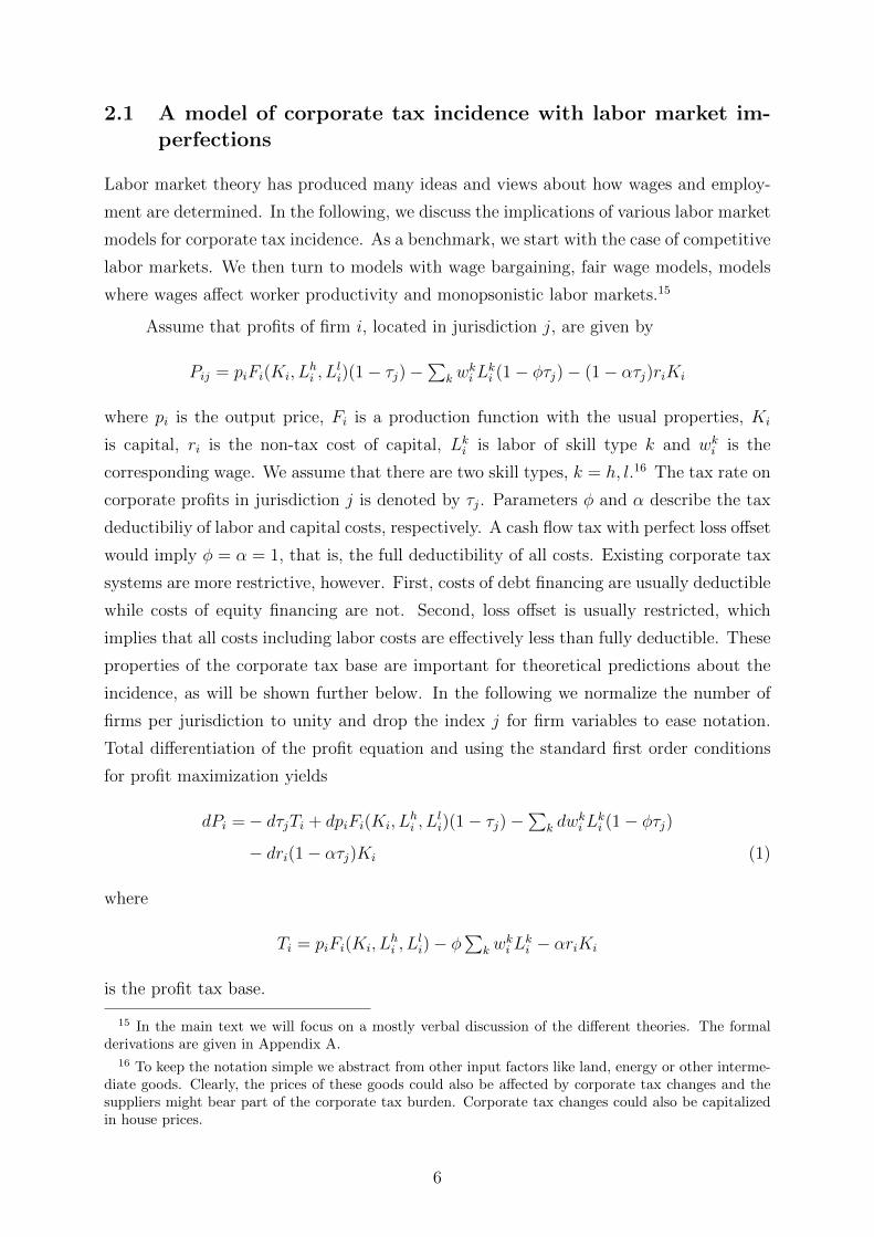
Assume that profits of firm i, located in jurisdiction j, are given by

Pij = piFi(Ki, Lhi , L

li)(1− τj)−

∑k w

ki L

ki (1− φτj)− (1− ατj)riKi

where pi is the output price, Fi is a production function with the usual properties, Ki

is capital, ri is the non-tax cost of capital, Lki is labor of skill type k and wki is the

corresponding wage. We assume that there are two skill types, k = h, l.16 The tax rate on

corporate profits in jurisdiction j is denoted by τj. Parameters φ and α describe the tax

deductibiliy of labor and capital costs, respectively. A cash flow tax with perfect loss offset

would imply φ = α = 1, that is, the full deductibility of all costs. Existing corporate tax

systems are more restrictive, however. First, costs of debt financing are usually deductible

while costs of equity financing are not. Second, loss offset is usually restricted, which

implies that all costs including labor costs are effectively less than fully deductible. These

properties of the corporate tax base are important for theoretical predictions about the

incidence, as will be shown further below. In the following we normalize the number of

firms per jurisdiction to unity and drop the index j for firm variables to ease notation.

Total differentiation of the profit equation and using the standard first order conditions

for profit maximization yields

dPi =− dτjTi + dpiFi(Ki, Lhi , L

li)(1− τj)−

∑k dw

ki L

ki (1− φτj)

− dri(1− ατj)Ki (1)

where

Ti = piFi(Ki, Lhi , L

li)− φ

∑k w

ki L

ki − αriKi

is the profit tax base.

15 In the main text we will focus on a mostly verbal discussion of the different theories. The formalderivations are given in Appendix A.

16 To keep the notation simple we abstract from other input factors like land, energy or other interme-diate goods. Clearly, the prices of these goods could also be affected by corporate tax changes and thesuppliers might bear part of the corporate tax burden. Corporate tax changes could also be capitalizedin house prices.

6

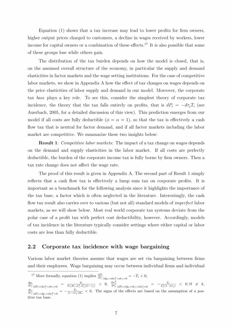
Equation (1) shows that a tax increase may lead to lower profits for firm owners,

higher output prices charged to customers, a decline in wages received by workers, lower

income for capital owners or a combination of these effects.17 It is also possible that some

of these groups lose while others gain.

The distribution of the tax burden depends on how the model is closed, that is,

on the assumed overall structure of the economy, in particular the supply and demand

elasticities in factor markets and the wage setting institutions. For the case of competitive

labor markets, we show in Appendix A how the effect of tax changes on wages depends on

the price elasticities of labor supply and demand in our model. Moreover, the corporate

tax base plays a key role. To see this, consider the simplest theory of corporate tax

incidence, the theory that the tax falls entirely on profits, that is dPi = −dτjTi (see

Auerbach, 2005, for a detailed discussion of this view). This prediction emerges from our

model if all costs are fully deductible (φ = α = 1), so that the tax is effectively a cash

flow tax that is neutral for factor demand, and if all factor markets including the labor

market are competitive. We summarize these two insights below:

Result 1: Competitive labor markets : The impact of a tax change on wages depends

on the demand and supply elasticities in the labor market. If all costs are perfectly

deductible, the burden of the corporate income tax is fully borne by firm owners. Then a

tax rate change does not affect the wage rate.

The proof of this result is given in Appendix A. The second part of Result 1 simply

reflects that a cash flow tax is effectively a lump sum tax on corporate profits. It is

important as a benchmark for the following analysis since it highlights the importance of

the tax base, a factor which is often neglected in the literature. Interestingly, the cash

flow tax result also carries over to various (but not all) standard models of imperfect labor

markets, as we will show below. Most real world corporate tax systems deviate from the

polar case of a profit tax with perfect cost deductibility, however. Accordingly, models

of tax incidence in the literature typically consider settings where either capital or labor

costs are less than fully deductible.

2.2 Corporate tax incidence with wage bargaining

Various labor market theories assume that wages are set via bargaining between firms

and their employees. Wage bargaining may occur between individual firms and individual

17 More formally, equation (1) implies dPi

dτj |dpi=dwki =dri=0

= −Ti < 0,

dpidτj |dPi=dwk

i =dri=0= Ti

Fi(Ki,Lhi ,L

li)(1−τj)

> 0,dwk

i

dτj |dPi=dpi=dri=dwli=0

= − Ti

Lki (1−φτj)

< 0,∀l 6= k,

dridτj |dPi=dpi=dwk

i =0= − Ti

(1−ατj)Ki< 0. The signs of the effects are based on the assumption of a pos-

itive tax base.

7

employees, but it may also take the form of collective bargaining, where employees are

represented by trade unions.

Bargaining models imply that firm owners and employees share a surplus generated

by the firm. If corporate taxes reduce this rent, it is natural to expect that part of the

loss is shared by employees through lower wages. The magnitude of these wage effects

depends on the level where bargaining takes place.

2.2.1 Individual wage bargaining

Assume that a firm hires a worker who generates a surplus Q and receives a wage w. The

wage is set via bargaining between the firm and the employee. The most widely used labor

market model where this happens is the job search model, in which firms and individual

employees bargain over a matching rent (see Rogerson et al., 2005, for a survey of labor

market search theories).

The available surplus after corporate taxes is given by Q(1 − τ) + wφτ . A tax

increase by dτ reduces the after-tax surplus before wage payments by Qdτ but the tax

change reduces the after-tax cost of wage payments by dτφw. A higher corporate tax

reduces the surplus the firm and the employee can share but the tax also “subsidizes”

wage payments. Here standard bargaining models like the Nash bargaining model imply

that each effect neutralizes the other if all costs are perfectly deductible. Existing tax

systems usually restrict the deductibility of costs through loss offset limitations or by

restricting capital allowances. In this case, part of the burden of a higher corporate tax is

passed on to employees. The effect increases with the bargaining power of the employee.

If the employee receives a large part of the surplus generated by the firm, it is plausible

that she also bears a large loss if the surplus declines due to taxation.

In Appendix A, we analyze the effect of a corporate tax change in a simple model

of bargaining between individual employees and firms. There we derive

Result 2: Individual wage bargaining : If wage or capital costs are less than fully

deductible, an increase (decline) in the local corporate tax rate reduces (increases) the

wage. The effect increases with the relative bargaining power of the employee.

2.2.2 Collective bargaining

Collective bargaining may take place at the firm-level, the sector-level or at the national

level. Taking into account the level at which wage bargaining takes place is particularly

important when it comes to analyzing the incidence of subnational level corporate taxes.

If the wage is set at the sector-level and the sector includes firms in many jurisdictions,

it is unlikely that a change in the local tax rate of one jurisdiction has a large effect on

8

wages. By contrast, if wages are set at the firm-level, a local tax change will have a larger

impact on wages.

In Appendix A, we consider both firm and sector-level collective bargaining. We

do so in a model where firms employ workers of different skill levels. Each skill group is

represented by a trade union. In the case of firm-level bargaining, we use the efficient

bargaining model (McDonald and Solow, 1981), where unions and individual firm owners

bargain over wages and employment. We denote the premium over the reservation wage

achieved through bargaining multiplied with the number of workers in a skill group as the

rent of the skill group. In the Appendix, we derive

Result 3: Firm-level bargaining : If either wage costs or capital costs are less than

fully deductible, an increase (decline) in the local corporate tax rate reduces (increases) the

rent of each skill group. For given levels of employment the wage rate declines (increases)

in response to an increase (decrease) in taxes (“direct effect” of a corporate tax change

on wages).

This result is similar to that of individual bargaining. Higher taxes reduce the rent

that can be shared between the firm and its employees. For given levels of employment,

wages unambiguously decline in response to a tax increase. In the literature, this effect has

been referred to as the ‘direct effect’ of a corporate tax change on wages in firms where

wages are set via collective bargaining (Arulampalam et al., 2012; Fuest et al., 2013).

Taking into account changes in employment may change the wage effect (indirect effect).

If the number of employees declines in response to a tax increase, the rent generated by

the company is shared among a smaller number of employees.

We now turn to models where collective bargaining takes place at the sector-level.

The efficient bargaining model used for firm-level bargaining is less suitable for sector-level

bargaining because bargaining over employment at the sector-level is difficult. We there-

fore use the seniority model proposed by Oswald (1993). The seniority model assumes

that union decisions are dominated by members who are interested in maximizing wages

and who are indifferent about the number of employed workers. As a consequence, a

sector-level union wants to maximize the sector wide wage rate while the employer repre-

sentation has the objective to maximize sector wide profits. After wages are determined,

firms set the profit maximizing level of employment. In such a setting, we derive

Result 4: Sector-level bargaining : If either wage costs or capital costs are less than

fully deductible, an increase in the tax rate may increase or decrease wages. The wage

effect converges to zero if the activity of the sector in the jurisdiction where the tax change

occurs is small, relative to the rest of the sector.

If wages are determined at the sector-level, and if the sector is present in many

9

jurisdictions, it is likely that a tax change in one jurisdiction will have a limited effect on

the sector wide wage. Nevertheless, it is still true that higher taxes reduce the after-tax

rent that is shared between firm owners and employees. How the decline in the rent is

translated into changes in wages and employment is theoretically ambiguous, as in the

case of firm-level bargaining.

Overall, the theory of collective bargaining does not generate unambiguous predic-

tions for how tax changes affect wages. In the empirical analysis, therefore, it would be

advisable to allow for differences in incidence effects for firm and sector-level bargaining.

If wages are set at the sector-level, a tax change should have a smaller effect on wages in

the jurisdiction than in the case where wage bargaining takes place at the firm-level.18

2.3 Corporate tax incidence in fair wage models

In fair wage models the wage is usually assumed to be a function of i) wages of other

employees of the same firm, ii) an external reference wage19, which can be the average

wage level paid in other firms, a statutory minimum wage or a transfer to the unemployed,

and iii) profits of the firm (see, e.g. Akerlof and Yellen, 1990). In general, employees of

a profitable firm will expect higher wages than those of a less profitable firm (see e.g.

Amiti and Davis, 2010; Egger and Kreickemeier, 2012). If higher corporate taxes reduce

after-tax profits, fairness considerations would suggest that employees will bear part of

this burden and vice versa. In Appendix A, we develop a simple fair wage model which

leads to

Result 5: Fair wage model : An increase (decline) in the local corporate tax rate

reduces (increases) the wages of all skill groups.

Note that Result 5 is independent of whether or not wage and capital costs are

fully deductible from the tax base. The neutrality property of cash flow taxes does not

hold here because wage fairness is assumed to depend directly on after-tax profits. The

fair wage model would also imply that collective wage bargaining may spill over to firms

without bargaining if they take the bargained wage as a reference point for fairness. This

could include wages in firms that do not pay the tax. Moreover, the model predicts that

the wage effects increases with the profitability of the firm.

18 Some labor markets are characterized by two tier bargaining, where sector-level bargaining sets aminimum wage and wage premiums on top of the minimum wage are negotiated at the firm-level (Boeri,2014). In a such a setting, one would expect local tax changes to have a more significant impact on localwages than in the case of pure sector-level wage bargaining.

19 We assume that the reference wage is given. it may of course be the case that the reference wage isaffected by local tax changes. This would not alter the result that higher taxes lead to lower wages andvice versa.

10

2.4 Corporate tax incidence in models where wages affect laborproductivity

Some labor market models emphasize that firms may raise wages because higher wages

lead to higher labor productivity and, hence, higher output. These models include effi-

ciency wage models, where higher wages lead to more effort or lower worker fluctuation,

and models of directed job search, where higher wages lead to better matches between

workers and firms.20 In Appendix A, we suggest a model where higher wages increase the

expected output of a firm because higher wages lead to better matches between workers

and firms (Acemoglu and Shimer, 1999).21 In this model, we derive

Result 6: Models where wages affect productivity : If either wage costs or capital

costs are less than fully deductible, an increase (decline) in the local corporate tax rate

reduces (increases) wages.

Result 6 can be explained as follows. The optimal wage trades off higher expected

output, which is taxed at the corporate tax rate τ , against the cost of higher wages, where

the tax deduction granted per unit of wage costs is φτ . In the presence of imperfect

deductibility (φ < 1), a tax rate increase by dτ reduces the after-tax benefit of a higher

expected output by a factor dτ and reduces the after-tax cost of wages only by φdτ . It is

therefore optimal for the firm to adjust its wage policy towards lower wages and a lower

quality of worker firm matches. Although the economic forces driving the wage setting

are different from those of wage bargaining models, the role of the tax deductibility of

wage costs is similar. In the polar case of perfect deductibility, corporate tax changes do

not affect wages.

2.5 Monopsonistic labor market

The model of monopsonistic labor markets is another widely used framework. To the

best our knowledge, it has, however, yet to be used to study corporate tax incidence.

In Appendix A, we suggest a simple model of a monopolistic labor market with a con-

stant elasticity of labor supply and a constant marginal productivity of labor.22 In this

20 The key difference to the fair wage model discussed in the preceding section is that the latteremphasizes the direct link between the profits of a firm and the wage that is perceived to be fair. Nosuch direct link exists here. However, fair wage models may also be considered as models where wagesaffect labor productivity because wages deemed as unfair would reduce worker effort or increase costlyfluctuation.

21 The results would be similar in an efficiency wage model following Solow (1979) with continuouseffort. In shirking models with discrete effort (such as Shapiro and Stiglitz, 1984) we would not expect adirect effect on wages (for given employment) but only an indirect effect though changes in unemploymentrates and hence the shirking constraint.

22 In the Appendix, we also consider a more general model where we relax the assumptions of a constantmarginal productivity of labor and a constant elasticity of labor supply. We also add capital to the model.

11

framework we derive

Result 7: Monopsonistic labor market : If either wage costs or capital costs are

less than fully deductible, an increase (decline) in the local corporate tax rate reduces

(increases) wages. The magnitude of the effect is increases with the elasticity of labor

supply.

Result 7 suggests that in monopsonistic labor markets groups of employees with a

higher elasticity of labor supply may paradoxically bear a higher share of the corporate

tax burden. This is because in monopsonistic wage settings, the wage is a share of the

marginal productivity of labor after-taxes. This share increases with the elasticity of

labor supply because a higher elasticity makes it more difficult for the firm to exploit its

market power. The higher share of the marginal product received by workers also means

that they lose more if the marginal product after-taxes declines.

2.6 Extensions

In this section, we consider two extensions of the model that are both related to particular

aspects of corporate taxation. The first extension takes into account that firms may

operate in more than one jurisdiction. Many countries use formula apportionment to

allocate corporate profits to different jurisdictions for taxation purposes. The second

extension is to allow for tax avoidance through income shifting between profits and wages

or between high and low tax jurisdictions.

2.6.1 Firms operating in multiple jurisdictions with formula apportionment

Consider a firm i with plants in 2 jurisdictions and assume for simplicity’s sake that there

is only one type of labor and that payroll is the only apportionment factor.23 In this

case, the firm’s profit tax rate is given by τi = τ1wL1+τ2wL2

wL1+wL2. If a jurisdiction increases

its tax rate, the effect on the firm’s profit tax rate τi can be small, depending on how

the firm’s payroll is distributed across jurisdictions. How such a tax change affects wages

and employment depends on the labor market setting and in particular on wage setting

institutions. In Appendix A, we analyze the case of firm-level collective bargaining since

this case is particularly relevant for our empirical analysis. We derive

Result 8: Formula apportionment and firm-level bargaining : In firms with plants in

many jurisdictions and homogeneous labor, where corporate taxation is based on formula

We show that the wage rate still unambiguously declines in response to a tax increase.23 This is the case for the local corporate tax in Germany. In the US, apportionment for state taxes

is based on payroll, sales and assets, see Suarez Serrato and Zidar (2014). The case for two skill types isdiscussed in Appendix A.

12

apportionment, and if wages are set via collective bargaining at the firm-level and either

wage or capital costs are less than fully deductible, an increase in the corporate tax rate

in one jurisdiction decreases wages in the entire firm. If employment in the jurisdiction

that changes the tax rate is small, relative to employment in the firm as a whole, the tax

effect is also small.

In the Appendix, we also consider the case of formula apportionment with two

skill types. In this case, the wage effect of corporate tax changes is ambiguous since wage

changes influence the effective tax rate of the firm, which in turn influences the bargaining

process. In the empirical analysis, the role of formula apportionment is investigated by

distinguishing between single and multi plant firms.

2.6.2 Income shifting to avoid taxes

Income shifting to avoid taxes may occur in different forms. Multinational firms can

use debt or transfer pricing to shift profits across national borders, from high to low tax

jurisdictions. This type of income shifting will dilute the effect of corporate tax changes

on wages because the tax base becomes smaller. However, income shifting may also

occur between different tax bases within a country. For instance, firm owners may shift

income between the corporate and the personal income tax base by changing wages paid

to family members. In this case, a higher corporate tax rate would lead to higher, not

lower reported wages. In Appendix A, we extend our model to allow for income shifting.

As done in the preceding section, we again focus on the case where wages are set via

firm-level bargaining.24 This leads to

Result 9 Income shifting : If firms engage in international income shifting and

wages are set by firm-level bargaining, then the decline in the rent accruing to labor

caused by a higher corporate tax decreases as the equilibrium level of income shifting

increases. If firms can shift income between the profit tax base and the labor income tax

base, reported wages will decline less than in the absence of income shifting or may even

increase in response to a higher corporate tax rate.

Result 9 implies that one would expect the observed effect of corporate tax changes

on wages to be smaller in multinational firms, where the tax impact is diluted by profit

shifting to other jurisdictions. Income shifting between the profit and the labor income tax

base within a jurisdiction would bring lower wage declines or even increases in response to

higher corporate taxes. This is likely to be relevant in very small firms, where higher taxes

on profits induce firm owners to report a higher share of profits as wages paid to family

24 As we explain in the appendix, income shifting between profits and wages may occur in the form ofmanipulating wages paid to family members of the owner employed by the firm. These wage paymentsare not determined via bargaining; rather they are effectively hidden profit distributions.

13

members employed by the company and where these employees represent a significant

share of the workforce.

3 Institutional background

We test the implications of our theoretical analysis exploiting the particular features of the

German corporate tax system. In Section 3.1, we briefly sketch the German business tax

system in general. Special emphasis is put on the local business tax (LBT, Gewerbesteuer).

This tax creates quasi-experimental variation in tax rates and is used for identification in

the empirical part of the paper. The key features of the nationwide corporate and personal

income taxes, the other two profit taxes in Germany, are described in Appendix B. In

Section 3.2, we document the cross-sectional and time variation of the LBT. Subsection

3.3 briefly discusses labor market institutions in Germany.

3.1 Business taxation in Germany

In 2007, profit taxes accounted for about 6.2% of total tax revenue (including social

security) in Germany (OECD, 2015) which is below the OECD average of about 10.6%

(US: 10.8%, UK 9.4%).25 There are three taxes on business profits in Germany, the

LBT, which is set by municipalities, the corporate tax (CT, Korperschaftsteuer) and the

personal income tax (PIT, Einkommensteuer), the latter two being levied by the federal

government. Corporate firms are liable to the LBT and the CT, while non-corporate firms

are liable to the LBT and the PIT. In terms of tax revenues, the LBT is the most important

profit tax, accounting for about 60–70% of total profit tax revenues from corporate firms.

The share of profit tax revenues from local taxes is relatively high in Germany compared

with other countries. In the US, for instance, state and local corporate taxes together

account only for about 20% of total corporate taxes (NCSL, 2009). In addition, the LBT

is the most important source of financing at the disposal of municipalities, generating

roughly three quarters of municipal tax revenue.

The LBT applies to both corporate and non-corporate firms, while most firms in the

agricultural and public sector are not liable. Moreover, certain liberal professions such as

journalists, physicians or lawyers are exempt. The tax base of the LBT is similar to that

of the corporate income tax.26 Taxable profits of firms with establishments in more than

25 Part of this relatively low share is due to the high importance of social security contribution (SIC)in Germany which is among the highest in the OECD. If SIC are excluded, the share in total taxes isabout 11.5%.

26 The most important difference is that interest payments are only partly deductible. Another differ-ence is that the LBT itself was a deductible expense until 2007.

14

one municipality are divided between municipalities according to formula apportionment

based on the payroll share.

The tax rate of the LBT, τLBT , consists of two components: the basic federal

rate (Steuermesszahl), τ fedLBT , which is set at the national level, and the local tax rate

(Hebesatz ), τmunLBT , which is set at the municipal level. The total LBT rate is given by

τLBT = τ fedLBT · τmunLBT . The basic federal rate, τ fedLBT , was at 5.0% from 1993 to 2007 and

decreased to 3.5% in 2008. The average local tax rate over our sample period (1993 –

2012) was 328%, yielding a total tax rate of 15.1%.

The local tax rates for year t are set by the municipal councils during the budgeting

process in the last three months of year t − 1. Each year the city council has a vote

about next year’s tax rate – even if it remains unchanged. It is important to note that a

municipality can adjust only the local tax rate that applies to all firms in the municipality.

It can not change the tax base, which is set at the federal level.

3.2 Variation in local business tax rates

In this subsection, we provide a detailed description of the variation in LBT rates. For our

analysis, we use administrative statistics provided by the Statistical Offices of the 16 Ger-

man federal states (Statistische Landesamter) on the fiscal situation of all municipalities.

We combine and harmonize the annual state specific datasets and construct a panel on

the universe of all municipalities from 1993 to 2012, covering 228,820 municipality years.

Most importantly, the dataset contains information on the local tax rate, but also on the

population size and municipal expenses and revenues. We also add data from the German

federal employment agency on regional unemployment rates on the more aggregate county

(Kreis) level to control for local labor market conditions.

Figure 1 depicts Germany’s 11,441 municipalities (according to 2010 boundaries)

and visualizes the substantial cross-sectional and time variation in local tax rates. The

left panel of the figure shows the cross-sectional variation in local tax rates in 2008 with

darker colors showing higher tax rates. Table C.1 in the appendix provides measures of

the distribution of LBT rates annually from 1993 to 2012. For the entire period, the

average local tax rate is 328%, while tax rates typically vary between 275% (P5) and

395% (P95).

We exploit the within-municipality variation in local tax rates over time to identify

the business tax incidence on wages. The right panel of Figure 1 demonstrates this

variation by showing the number of tax changes a municipality during the period 1993–

2012 (with darker colors indicating more changes). Table C.2 in the Appendix shows the

corresponding numbers. Overall, only 15% of the municipalities did not experience a tax

15

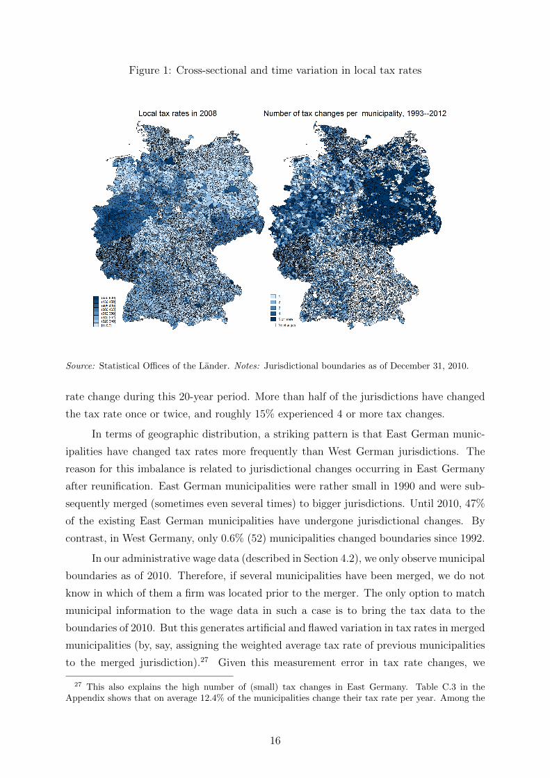
Figure 1: Cross-sectional and time variation in local tax rates

Source: Statistical Offices of the Lander. Notes: Jurisdictional boundaries as of December 31, 2010.

rate change during this 20-year period. More than half of the jurisdictions have changed

the tax rate once or twice, and roughly 15% experienced 4 or more tax changes.

In terms of geographic distribution, a striking pattern is that East German munic-

ipalities have changed tax rates more frequently than West German jurisdictions. The

reason for this imbalance is related to jurisdictional changes occurring in East Germany

after reunification. East German municipalities were rather small in 1990 and were sub-

sequently merged (sometimes even several times) to bigger jurisdictions. Until 2010, 47%

of the existing East German municipalities have undergone jurisdictional changes. By

contrast, in West Germany, only 0.6% (52) municipalities changed boundaries since 1992.

In our administrative wage data (described in Section 4.2), we only observe municipal

boundaries as of 2010. Therefore, if several municipalities have been merged, we do not

know in which of them a firm was located prior to the merger. The only option to match

municipal information to the wage data in such a case is to bring the tax data to the

boundaries of 2010. But this generates artificial and flawed variation in tax rates in merged

municipalities (by, say, assigning the weighted average tax rate of previous municipalities

to the merged jurisdiction).27 Given this measurement error in tax rate changes, we

27 This also explains the high number of (small) tax changes in East Germany. Table C.3 in theAppendix shows that on average 12.4% of the municipalities change their tax rate per year. Among the

16

focus on non-merged municipalities in our baseline analysis (and check whether results

for merged and non-merged municipalities differ). Due to this restriction, we are left with

about 10,000 municipalities and 18,000 tax changes for identification (instead of 11,441

municipalities with about 27,000 partly artificial tax changes).

Table C.3 shows that 94% of tax changes are tax increases, with the average increase

being 23 percentage points (of τmunLBT ).28 Evaluated at the mean local tax rate of 328% and

for a given federal business tax rate, this rise implies an increase of the total business tax

rate by 7% (or 1.15 percentage points for an average total tax rate of 16.4%). Hence, we

exploit quite a few tax reforms with fairly large scopes for identification.

3.3 German labor market institutions

As our theoretical predictions depend on underlying wage setting institutions, we briefly

describe the German labor market.29 Traditionally, German labor unions have been very

influential. Collective bargaining agreements (CBAs) at the sector-level are the most

important mechanism for wage determination. Nevertheless, there has been a significant

decline in bargaining coverage. In West (East) Germany, CBA coverage decreased from

76% (63%) in 1998 to 65% (51%) in 2009. The share of workers covered by sectoral

agreements fell from 68% (52%) to 56% (38%) (Ellguth et al., 2012).30 In addition to

sector-level CBA, some firms have firm-level agreements, while other firms are not covered

by a CBA and rely on individual contracts with each employee.

The average duration of a CBA increased from 12 months in 1991 to 22 months in

2011. Usually, negotiations take place in the first half of a year. Firms may pay wages

above those negotiated in CBAs. Note that except for a few industries, there was no legal

minimum wage in Germany during our period of analysis. However, the social security

and welfare system provides an implicit minimum wage and CBAs ensure that wages are

above that level.

merged municipalities, however, the share is 33% (with a much smaller average change).28 In light of the vast international evidence of decreasing tax rates for companies, this seems surprising

at first sight. Yet, both the CT rate and the top PIT rate decreased over the period 1993–2012 so thatthe overall tax rate for companies decreased as well (see Appendix B for more details). Thus, a rise inthe LBT rates in a municipality over time has to be seen as a slower decrease in overall tax burdens forfirms in these municipalities than with those of firms in other jurisdictions with stable local tax rates.

29 See, e.g., Dustmann et al. (2014) for an overview and analysis of the development of German labormarket institutions during our period of investigation.

30 Coverage rates vary by industry: collective bargaining is slightly above average in the manufacturingsector, while the highest coverage is in the public sector and the lowest in ICT, agriculture and restaurantindustries). Overall, union coverage rates in Germany are lower than in other European countries – exceptthe UK and some Eastern European countries – but higher than in the US (Du Caju et al., 2008).

17

4 Empirical strategy and data

4.1 Empirical model and identification

We implement an event study design to estimate the effect of changes in the local tax

rate on wages. Our baseline outcome variable is the log median real wage in firm f ,

municipality m, and year t, wp50fm,t. Note that each municipality is nested in a county c,

commuting zone r and state s. We choose the median as the baseline to account for the

top-coding of wages at the ceiling for social security contributions, which affects up to

13% of wage earners (see the discussion in the next subsection). Nevertheless, we also use

the 25% percentile and the 75% percentile as well as the mean wage as outcome variables

to assess the distributional effects of the reform and check the sensitivity of our estimates.

In the context of our study, we make two adaptations to the conventional event

study design (Sandler and Sandler, 2014). First, we take into account that there may be

multiple tax changes over time per municipality. Second, tax changes differ in size (and

sign). Hence, instead of regressing the wage in period t on dummy variables indicating tax

reforms, we multiply the reform dummies with the respective tax rate change. Formally,

our model reads:

lnwp50fm,t = γ−b

B−t∑i=b

∆τm,t+i +a−1∑

j=−b+1

γj∆τm,t−j + γa

t−A∑k=a

∆τm,t−k

+ µf + µm + µt + εfm,t, (2)

The coefficients of interest are the γ’s, which measure the wage effect in t of tax

reforms occurring in the event window between t − a years in the past to t + b years

in the future. The regressor ∆τm,t+j is the change in the local tax rate of municipality

m from t + j − 1 to t + j.31 Given wage data from 1998 to 2008 (see Section 4.2), we

set b = 4 and a = 5 allowing us to cover ten years around a tax reform occurring in

period t = 0.32 A pre-treatment period of 4 years seems long enough to detect potential

pre-trends while 5 years after treatment suffice to look beyond the short-run effects of the

reforms.33 We adjust the ends of the event window (coefficients γ−b and γa) to take into

account tax changes that are outside of the event window, which runs from t− a to t+ b.

The first and the last data year are denoted A and B, respectively. Given our sample, it

31 Note that this is equivalent to taking a dummy variable indicating a tax rate change from t+ j − 1to t+ j and interacting it with the corresponding change.

32 The choice of this event window implies that we need tax data from 1993 until 2012, see Section 3.2.33 We experimented with different leads and lags, but the results proved to be stable.

18

follows that A = 1993, B = 2012. The specification makes the set of a + b + 1 regressors

perfectly collinear. We drop the regressor for the pre-reform year (and normalized it to

zero). Hence, all coefficients have to be interpreted relative to the pre-reform year. We

also include municipal, µm, firm, µf , and year fixed effects µt, to our equation.34 The

error term is denoted by εm,t.

In order to test for heterogeneous effects, we interact the tax rate changes ∆τm,t+j, j =

−b, ..., a, with firm or worker characteristics. Note that some of those characteristics such

as collective bargaining agreement or single vs. multi establishment firm are potentially

endogenous and may respond to the tax rate. For this reason, we fix the characteristics

to the values of 1997, i.e., the year prior to our first panel observation.

Identification Given that the model includes firm and municipal fixed effects, we iden-

tify the effect of tax changes on wages within firms and municipalities over time. We thus

estimate a variant of a difference-in-differences model with fixed effects. As usual, the γ

coefficients measure the causal effect of local tax rates on wages provided that there is

neither reverse causality nor omitted variable bias.

The coefficients on future tax changes can be used to directly check for reverse

causality problems in the spirit of a Granger test. Identification requires a flat trend –

that is, no statistically significant wage responses – preceding a tax reform. With respect

to omitted confounders, our research design would be invalid if local shocks systematically

affected tax rates and wages. We provide two checks to assess whether such potential local

shocks are likely to bias our estimates. First, we run event study designs as specified in

equation (2) using municipal unemployment, county GDP and municipal fiscal surplus

as outcome variables. Significant pre-treatment trends for these outcomes would hint at

local shocks and cast doubt on our identifying assumption. As will be shown in Section

5.1, there are no local shocks to the business cycle prior to a tax reform.

As a second test, we enhance the model shown in equation (2) to directly take into

account local shocks. Instead of including simple year fixed effects, we include “state

× year” fixed effects – which account for any shock omitted at the state-level, such as

municipal election years, which have recently been shown to affect LBT rates (Foremny

and Riedel, 2014). In a more involved specification, we include fixed effects “commuting

zone × year”. German municipalities are nested in 258 commuting zones, which are

delineated by commuter flows. Adding these 258 · 11 = 2838 dummy variables, takes

out annual labor market shocks at the local level. Besides these purely non-parametric

specifications, we also estimate a model where we directly account for local time-varying

34 Note that firm and municipal fixed effects are highly collinear as only very few firms move betweenmunicipalities in the data.

19

confounders by adding lagged county GDP, unemployment and municipal revenues to

equation (2). If there was an omitted variable problem in our baseline specification, we

would expect coefficients to change substantially after controlling for these variables as

they should be correlated with local shocks.

Worker level estimations. We also implement an event study design at the individual

level to test for heterogeneous effects. The empirical model for the worker-level equations

is defined as follows:

lnwifm,t = γ−b

B−t∑i=b

∆τm,t+i +a−1∑

j=−b+1

γj∆τm,t−j + γa

t−A∑k=a

∆τm,t−k

+ µi + µf + µm + ψt + εifm,t, (3)

Here the outcome variable is the log wage of individual i, working in firm f that is situated

in municipality m. We also add individual fixed effects to the model, so identification

remains within individual-firm-municipality combinations.35

Inference. Usually, we cluster standard errors at the municipal level, i.e. the level of

our identifying variation. Given the well-known problems of biased standard errors in

difference-in-difference models (Bertrand et al., 2004), we conduct two tests to assess the

sensitivity of our estimates: First, we aggregate the data to the municipal level and re-

estimate equation (2) finding similar results. Second, we follow the suggestions by Angrist

and Pischke (2009) to “pass the buck up one level” and cluster standard errors on a higher

level of aggregation, which in our case is the county or the commuting zone. Standard

errors of estimates are hardly affected (see Appendix D for both checks).

4.2 Linked employer-employee data

We combine the administrative municipal data presented in Section 3.2 with linked

employer-employee data (LIAB) provided by the Institute of Employment Research (IAB)

in Nuremberg, Germany (Alda et al., 2005). The LIAB combines administrative worker

data with firm-level data.

The firm component of the LIAB is the IAB Establishment Panel (Kolling, 2000),

which is a stratified random sample of all German establishments. The term establishment

35 Technically, we apply the spell fixed-effects estimator suggested by Andrews et al. (2006) whenestimating equations (2) and (3) and de-mean variables within each unique (worker-)firm-municipalitycombination.

20

refers to the fact that the observational unit is the individual plant, not the firm. The

employer data covers establishments with at least one worker subject to social insurance

contributions. The sample covers about 15,000 establishments, which corresponds to

about 1% of all German establishments. We extract the following variables: value added,

investment, number of employees, industry, total wage bill, legal form, union wage status

(industry, firm or no collective agreement) and self-rated profitability36

In addition to the plant-level information, the data set contains information on all

employees in the sampled establishments. The employee data is taken from the adminis-

trative employment register of the German Federal Employment Agency (Bundesagentur

fur Arbeit) covering all employees paying social security contributions (Bender et al.,

2000).37 The employee information are recorded on June 30th of each year and include

information on wages, age, tenure, occupation, employment type (full-time or part-time

employment) and qualification. Individuals with missing information are excluded. Our

worker panel consists of between 1.6 and 2.0 million workers (corresponding to about 6%

of all workers) annually observed from 1998 to 2008. The choice of years is driven by data

availability for the tax rate data to allow for a sufficient number of years before and after

the tax reforms. Furthermore, ending in 2008 avoids the effects of the Great Recession.

Importantly, wages are right censored at the ceiling for social security contributions.

Although the ceiling is quite high, with annual labor earnings of 63,400 euros in 2008 for

Western Germany, up to 13% of the observations are censored. Note that the censoring

does not affect results on the firm-level since we use the median wage in the establishment

as our left-hand-side variable. At the individual level, we opt for a conservative approach

and assign censored individuals the cap leading to an underestimate of the wage effect.

As a sensitivity check, we exclude all individuals who at least once earned a wage above

the contribution ceiling during the observation period.38 As shown below, this exclusion

affects the results for high-skilled workers.39

36 The survey question asks for a self-assessment of the profit situation on a five-point scale rangingfrom very good to unsatisfactory. We pool the two answers “very good” and “good” as well as “fair” and“poor” and construct a three-point scale (high, medium, low) for profitability with well-balanced supportover the three categories.

37 Note that civil servants, self-employed individuals and students are not observed in the social securitydata. The data nonetheless contain more than 80% of all employed persons in Germany.

38 Imputing censored wages is a third option used in the literature (Dustmann et al., 2009; Card et al.,2013). While imputing censored wages using a Tobit procedure is sensible when analyzing wage inequality,it is problematic in our study, in which we use the individual wage as the left-hand-side variable. In fact,the LBT rate would have to be a regressor in both the Tobit model and the even study design.

39 We differentiate between three skill groups: high-skilled workers who have obtained a col-lege/university degree; medium-skilled who have completed either vocational training or the highesthigh school diploma (Abitur); low-skilled who have completed neither of the two.

21

Descriptive statistics. Appendix Tables C.4, and C.5 present descriptive statistics of

our plant and worker level sample.40 Table C.4 shows that the average median firm wage

is 2,555 euros. 15% of our municipality-year observations have undergone either a tax

increase or a tax decrease, with an average local tax rate of 371%. The average (median)

size of the municipality is 98,613 (26,456) inhabitants. About three quarters of the sample

are municipalities that have not undergone a merger between 1993 and 2012. The average

(median) plant has 239 (52) employees. 64% of the plants are liable to the LBT and about

60% of the firms are liable to the corporate tax. Most of the establishment are single-plant

firms. More than half of the firms have sector-level bargaining agreements in place.

Not surprisingly, we observe more workers in larger firms. As larger firms pay higher

wages, we see that the average wage in the individual level sample increases to 3,358 euros

per month (see Table C.5). The average (median) number of workers increases to 4,875

(908). In terms of individual characteristics, the table shows that the average worker in

our sample is 42 years old. The share of males is 71%. 14% of the individuals are high

skilled, while about as many are low-skilled. 83% of the individuals have never earned a

wage higher than the social security contribution cap in our sample.

5 Empirical results

In this section, we estimate the incidence of corporate taxation on wages. Before turn-

ing to our main results, we test our identifying assumption by analyzing whether local

productivity shocks affect tax rate changes.

5.1 Drivers of local tax rate changes

While it is common to use variation in policies across regions and over time to identify

policy effects, the approach requires the exogeneity of the policy change with respect to

the outcome variables. A particular concern in our setting is whether tax rates respond

to local business cycle shocks, which could also affect wages.41 Analyzing pre-trends in

our event study design provides a first test of the identifying assumption. As will be

shown below, wage rates do not change significantly prior to tax changes. In addition,

we can test directly for violations of the identifying assumptions by using local economic

outcomes as left-hand-side variables in the event study model. In particular, we test

40 In the baseline, we only consider full-time workers. We also looked at the effects on part-time wagesbut find no significant differences, see the discussion in Section 5.4.

41 Previous evidence for the German LBT (Foremny and Riedel, 2014) as well as for income tax reformsin Europe (Castanheira et al., 2012) suggest that tax changes are typically triggered by political concerns,not economic variables.

22

whether unemployment, GDP and fiscal surplus change prior to tax reforms.

Panel A of Appendix Figure D.5 shows that municipal unemployment levels are flat

prior to a tax reform. Similarly, Panel A of Appendix Figure D.6 shows no significant

pre-trends for GDP.42 While we find no evidence of significant pre-trends, we do find that

county GDP declines after the reform. Likewise, there is an increase in unemployment

rates. However, while both effects are statistically significant, they are economically very

small in magnitude (each change being about 0.02%).43

In Panel B of Appendix Figure D.6, we show the evolution of fiscal surpluses per

capita before and after a tax change. While pre-trends are again remarkably flat, we find

a small and insignificant increase of 18 euros per capita in the fiscal surplus in the year

of the tax increase. It seems that this fiscal surplus will be “eaten up” by a small deficit

of 6 euros per capita in years 1 to 3 after a tax increase. While the effect is quite small,

we nevertheless include local expenditures in some specifications to test the robustness

of our results when accounting for potentially improved public services in a municipality

with increasing local tax rates. We find that results do not change in that case.

5.2 Baseline results

In this section, we present our main results obtained from estimating equation (2). We

present results graphically plotting the γ coefficients and the corresponding 95% confi-

dence intervals. Regression tables are provided in Appendix E. As discussed in Section

3.2, we focus on the 10,000 municipalities that did not changes jurisdictional borders be-

tween 1993 and 2012.44 For our baseline estimate, we focus on firms that are liable to the

LBT. Figure 2 depicts the results. Pre-reform trends are flat and not statistically different

from zero. After a change in the municipal business tax rate in period 0 (indicated by

the vertical red line), real wages start to decline and are 0.047 log points below the pre-

reform year five years after the reform. The coefficient corresponds to a wage elasticity

with respect to the LBT rate of 0.14. In Section 5.5, we show that this central estimate

implies that a 1-euro increase in the tax bill leads to a 0.56-euro decrease in the wage bill.

Figure 2 also contains information about firms that are exempt from the LBT. We find

positive yet insignificant wage effects.45 In the following, we consider the results for liable

42 Note that local GDP data are available at the county level but not at the municipal level. In orderto show that moving to a more aggregate level does not drive the results, Panels A and B of Figure D.5depict unemployment results when running the analysis on the municipal vs. the county level. There areonly small differences.

43 In a companion paper, Siegloch (2013) further investigates the (un)employment effects of the LBT.44 Nevertheless, we present results for merged municipalities in Figure D.1 in Appendix D.45 If non-liable firms were not affected at all by the tax increase the difference between the two curves

would be the treatment effect. However, we cannot be sure that exempted firms are a valid control group

23

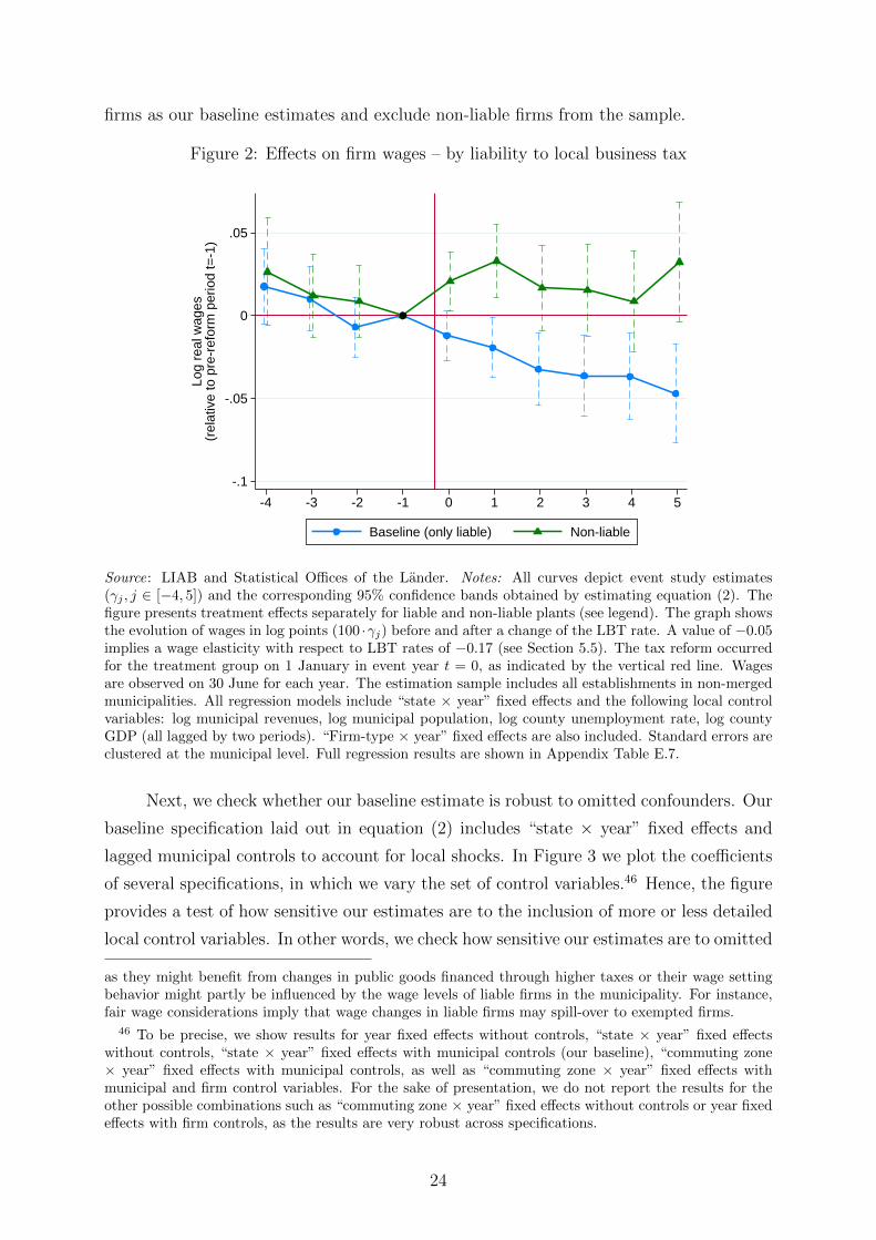
firms as our baseline estimates and exclude non-liable firms from the sample.

Figure 2: Effects on firm wages – by liability to local business tax

-.1

-.05

0

.05

Log

real

wag

es(r

elat

ive

to p

re-r

efor

m p

erio

d t=

-1)

-4 -3 -2 -1 0 1 2 3 4 5

Baseline (only liable) Non-liable

Source: LIAB and Statistical Offices of the Lander. Notes: All curves depict event study estimates(γj , j ∈ [−4, 5]) and the corresponding 95% confidence bands obtained by estimating equation (2). Thefigure presents treatment effects separately for liable and non-liable plants (see legend). The graph showsthe evolution of wages in log points (100 ·γj) before and after a change of the LBT rate. A value of −0.05implies a wage elasticity with respect to LBT rates of −0.17 (see Section 5.5). The tax reform occurredfor the treatment group on 1 January in event year t = 0, as indicated by the vertical red line. Wagesare observed on 30 June for each year. The estimation sample includes all establishments in non-mergedmunicipalities. All regression models include “state × year” fixed effects and the following local controlvariables: log municipal revenues, log municipal population, log county unemployment rate, log countyGDP (all lagged by two periods). “Firm-type × year” fixed effects are also included. Standard errors areclustered at the municipal level. Full regression results are shown in Appendix Table E.7.

Next, we check whether our baseline estimate is robust to omitted confounders. Our

baseline specification laid out in equation (2) includes “state × year” fixed effects and

lagged municipal controls to account for local shocks. In Figure 3 we plot the coefficients

of several specifications, in which we vary the set of control variables.46 Hence, the figure

provides a test of how sensitive our estimates are to the inclusion of more or less detailed

local control variables. In other words, we check how sensitive our estimates are to omitted

as they might benefit from changes in public goods financed through higher taxes or their wage settingbehavior might partly be influenced by the wage levels of liable firms in the municipality. For instance,fair wage considerations imply that wage changes in liable firms may spill-over to exempted firms.

46 To be precise, we show results for year fixed effects without controls, “state × year” fixed effectswithout controls, “state × year” fixed effects with municipal controls (our baseline), “commuting zone× year” fixed effects with municipal controls, as well as “commuting zone × year” fixed effects withmunicipal and firm control variables. For the sake of presentation, we do not report the results for theother possible combinations such as “commuting zone × year” fixed effects without controls or year fixedeffects with firm controls, as the results are very robust across specifications.

24

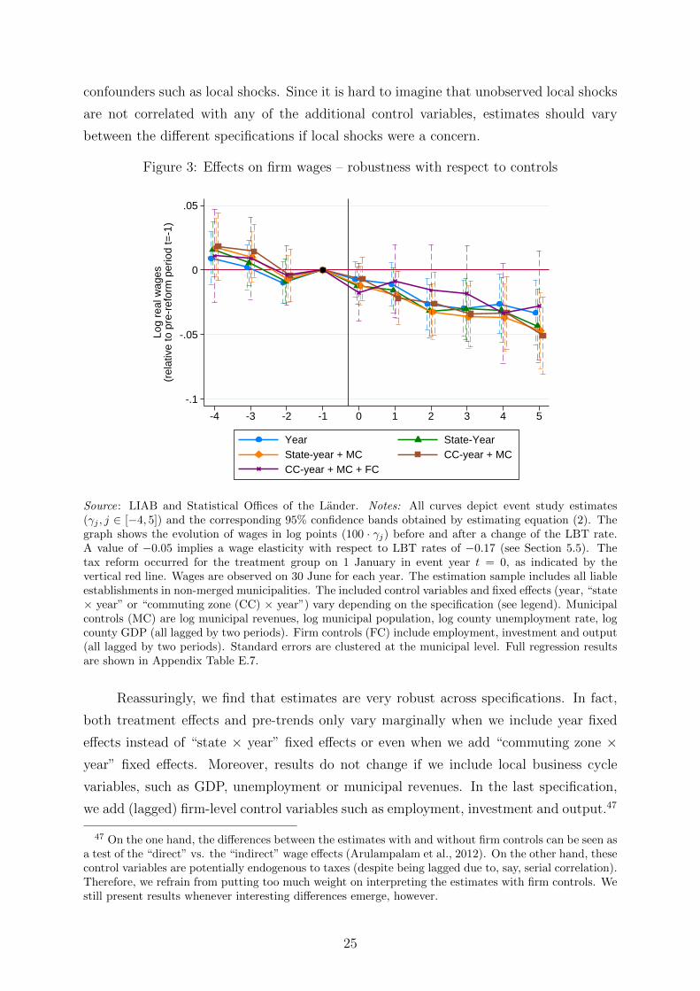
confounders such as local shocks. Since it is hard to imagine that unobserved local shocks

are not correlated with any of the additional control variables, estimates should vary

between the different specifications if local shocks were a concern.

Figure 3: Effects on firm wages – robustness with respect to controls

-.1

-.05

0

.05

Log

real

wag

es(r

elat

ive

to p

re-r

efor

m p

erio

d t=

-1)

-4 -3 -2 -1 0 1 2 3 4 5

Year State-YearState-year + MC CC-year + MCCC-year + MC + FC

Source: LIAB and Statistical Offices of the Lander. Notes: All curves depict event study estimates(γj , j ∈ [−4, 5]) and the corresponding 95% confidence bands obtained by estimating equation (2). Thegraph shows the evolution of wages in log points (100 · γj) before and after a change of the LBT rate.A value of −0.05 implies a wage elasticity with respect to LBT rates of −0.17 (see Section 5.5). Thetax reform occurred for the treatment group on 1 January in event year t = 0, as indicated by thevertical red line. Wages are observed on 30 June for each year. The estimation sample includes all liableestablishments in non-merged municipalities. The included control variables and fixed effects (year, “state× year” or “commuting zone (CC) × year”) vary depending on the specification (see legend). Municipalcontrols (MC) are log municipal revenues, log municipal population, log county unemployment rate, logcounty GDP (all lagged by two periods). Firm controls (FC) include employment, investment and output(all lagged by two periods). Standard errors are clustered at the municipal level. Full regression resultsare shown in Appendix Table E.7.

Reassuringly, we find that estimates are very robust across specifications. In fact,

both treatment effects and pre-trends only vary marginally when we include year fixed

effects instead of “state × year” fixed effects or even when we add “commuting zone ×year” fixed effects. Moreover, results do not change if we include local business cycle

variables, such as GDP, unemployment or municipal revenues. In the last specification,

we add (lagged) firm-level control variables such as employment, investment and output.47

47 On the one hand, the differences between the estimates with and without firm controls can be seen asa test of the “direct” vs. the “indirect” wage effects (Arulampalam et al., 2012). On the other hand, thesecontrol variables are potentially endogenous to taxes (despite being lagged due to, say, serial correlation).Therefore, we refrain from putting too much weight on interpreting the estimates with firm controls. Westill present results whenever interesting differences emerge, however.

25

Results are again broadly similar with somewhat lower point estimates and larger standard

errors.48 These are due to interesting differences from industry to industry (see below).

Furthermore, our results are also robust to including future and current municipal

expenses as control variables (not shown). Such a specification shuts down one theoretical

channel that might lead to a wage response from a tax reform. As discussed in Section 2,

higher taxes might lead to higher municipal spending and thus better local public services,

which in turn might generate lower wages in the form of a compensating differential. As

estimates remain unchanged when adding local controls, this channel does not appear

to be empirically relevant in Germany. In comparing all curves, it becomes evident that

controlling for local shocks does not affect wage adjustment.

Sensitivity checks. We conduct several sensitivity checks to test the robustness of our

baseline results. First, we address the issue of wage censoring. As described in Section

4.2, wages are censored at the ceiling for social security contributions. For this reason, we

choose the log median wage in firm f , which is invariant to the censoring, as our left-hand-

side variable. In Figure D.2 in Appendix D, we test whether this choice affects results by

using the mean wage in firm f instead of the median. Moreover, we test whether different

parts of the wage distribution within firms are affected differently by replacing the log

median wage with the log P25 and P75 wage.

Figure D.2 shows the negative wage effects that also arise when using the mean

wage at the establishment level. But these effects are smaller, which suggests that wage

censoring leads to a downward bias of our estimate.49 Moreover, we find that negative

wage effects for the top 25% of wage earners in each firm are significantly lower. There

are two potential explanations for this finding. First, while up to 13% of workers earn

wages above the social security contribution ceiling, the share of censored workers might

be higher than 25% in certain firms. If this were the case, lower estimates could have

resulted from the downward bias induced by wage censoring. Second, it is possible that

higher income earners within a firm are more mobile, which should lead to lower wage

responses.

In our baseline model, standard errors are clustered at the municipal level. Given the

well-known problems of biased standard errors in difference-in-difference models (Bertrand

et al., 2004), we first estimate an event study regression on the municipal level, using the

median municipal wage as our left-hand-side variable and clustering at the municipal

level. While estimates are a bit more noisy and less stable due to smaller numbers of

48 Results are also similar when adding the control variables – either on the municipal or firm-level –sequentially or in turn instead of all together.

49 Note that we corroborate this hypothesis below, when running event studies on the worker level.

26

observations and the fact that the wage measures includes liable and non-liable firms,

effects are still comparable (see Figure D.3 in the Appendix). Second, when clustering at

higher levels of aggregation, we find that the significance of our estimates hardly changes

(see Table D.6 in the Appendix).

5.3 Heterogeneous firm effects

In the following sections, we test for heterogeneous firm and worker effects. By doing this

we try to get at the underlying mechanisms driving wage responses to tax rate changes

and relate these back to our theoretical considerations.

First, we test for differences in terms of industry (Figure 4). Interacting the event

dummy regressors with industry dummies, the solid lines in Panel A show that effects

for manufacturing and services are quite similar after 4 to 5 years. However, wages in

the manufacturing sector seem to respond immediately, while service sector firms start

to pay lower wages after 2 to 3 years. These different adjustment paths could be due

to different labor market institutions: the labor market in the service sector is much

more competitive, while unions are strong in the manufacturing sector. According to our

theoretical model, the difference in adjustment paths could be driven by the differences in

direct and indirect effects across sectors. While the direct bargaining effect (conditional on

factor inputs) can be expected to be more relevant for manufacturing firms, indirect effects

induced by changes in factor inputs could dominate in the service sector. To test this

hypothesis, we re-estimate the model conditional on output, employment and investment,

which empirically shuts down the indirect effect (with the caveats discussed in footnote

47). Indeed the dashed lines in Panel A suggest that the wage effect in the service sector

is driven by the indirect effect. By contrast, wage effects in the manufacturing sector are

scarcely affected by eliminating production factor adjustments, which suggests that the

direct effect is more important in this sector. A possible interpretation of these findings is

that wage effects in manufacturing reflect rent sharing while higher taxes induce service

sector firms to relocate jobs to other jurisdictions, so that local wages decline.

The sectoral results might also be interpreted as shedding light on the role of price

effects in our setting. Comparing the manufacturing sector, which mostly produces highly

tradable goods, to the service sector, where goods are arguably less tradable, we see no

significant differences in the overall wage response. If price effects indirectly affected wage

responses, we should observe differences in wage effects by sector.

27

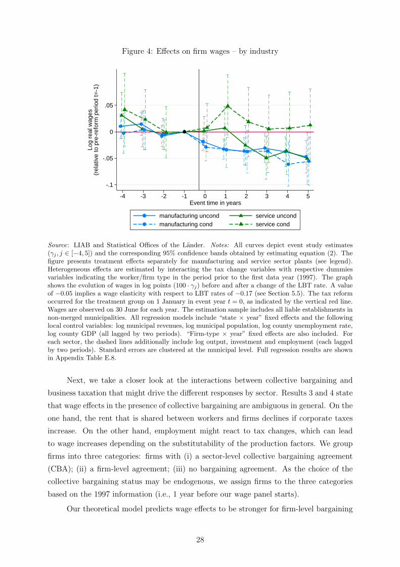
Figure 4: Effects on firm wages – by industry

-.1

-.05

0

.05

Log

real

wag

es(r

elat

ive

to p

re-r

efor

m p

erio

d t=

-1)

-4 -3 -2 -1 0 1 2 3 4 5Event time in years

manufacturing uncond service uncondmanufacturing cond service cond

Source: LIAB and Statistical Offices of the Lander. Notes: All curves depict event study estimates(γj , j ∈ [−4, 5]) and the corresponding 95% confidence bands obtained by estimating equation (2). Thefigure presents treatment effects separately for manufacturing and service sector plants (see legend).Heterogeneous effects are estimated by interacting the tax change variables with respective dummiesvariables indicating the worker/firm type in the period prior to the first data year (1997). The graphshows the evolution of wages in log points (100 · γj) before and after a change of the LBT rate. A valueof −0.05 implies a wage elasticity with respect to LBT rates of −0.17 (see Section 5.5). The tax reformoccurred for the treatment group on 1 January in event year t = 0, as indicated by the vertical red line.Wages are observed on 30 June for each year. The estimation sample includes all liable establishments innon-merged municipalities. All regression models include “state × year” fixed effects and the followinglocal control variables: log municipal revenues, log municipal population, log county unemployment rate,log county GDP (all lagged by two periods). “Firm-type × year” fixed effects are also included. Foreach sector, the dashed lines additionally include log output, investment and employment (each laggedby two periods). Standard errors are clustered at the municipal level. Full regression results are shownin Appendix Table E.8.

Next, we take a closer look at the interactions between collective bargaining and

business taxation that might drive the different responses by sector. Results 3 and 4 state

that wage effects in the presence of collective bargaining are ambiguous in general. On the

one hand, the rent that is shared between workers and firms declines if corporate taxes

increase. On the other hand, employment might react to tax changes, which can lead

to wage increases depending on the substitutability of the production factors. We group

firms into three categories: firms with (i) a sector-level collective bargaining agreement

(CBA); (ii) a firm-level agreement; (iii) no bargaining agreement. As the choice of the

collective bargaining status may be endogenous, we assign firms to the three categories

based on the 1997 information (i.e., 1 year before our wage panel starts).

Our theoretical model predicts wage effects to be stronger for firm-level bargaining

28

than for sector-level bargaining – especially if the sector has a presence in many munici-

palities (cf. Result 4). Panel A of Figure 5 tests this prediction. We find that firms with a

firm-level CBA show a much stronger negative wage effect than firms with sector-level bar-

gaining. Nevertheless, we see a negative (yet insignificant) wage response for sector-level

firms as well as for no-bargaining firms. In the following we analyze this modest decrease

in more detail. As above, we try to recover the direct wage effect by re-estimating the

model conditional on employment, investment and output so as to eliminate the indirect

wage effects. In line with the theoretical predictions, we do not detect a direct wage

effect for non-bargaining firms. Results for firms with CBAs are very similar, which again

suggests that direct effects dominate in firms with labor unions.

In the next step, we take into account the fact that not all sector-level bargaining

agreements are binding. Sector-level CBAs set a wage floor and firms are allowed to pay

above the union wage. We observe whether or not firms pay wages above the bargaining

agreement. Moreover, we can distinguish whether firms without a CBA peg their wages to

a union contract, which can be rationalized with a fair wage model. Results are depicted

in Panel B of Figure 5. In line with our theory, we only find negative wage effects in firms

for which the sector-level CBA is not binding. In addition, we find that firm without

bargaining tend to respond more strongly if they follow a sector-level agreement and pay

wages above the union wage. This can be interpreted as reflecting fairness considerations

in the wage setting process.

29

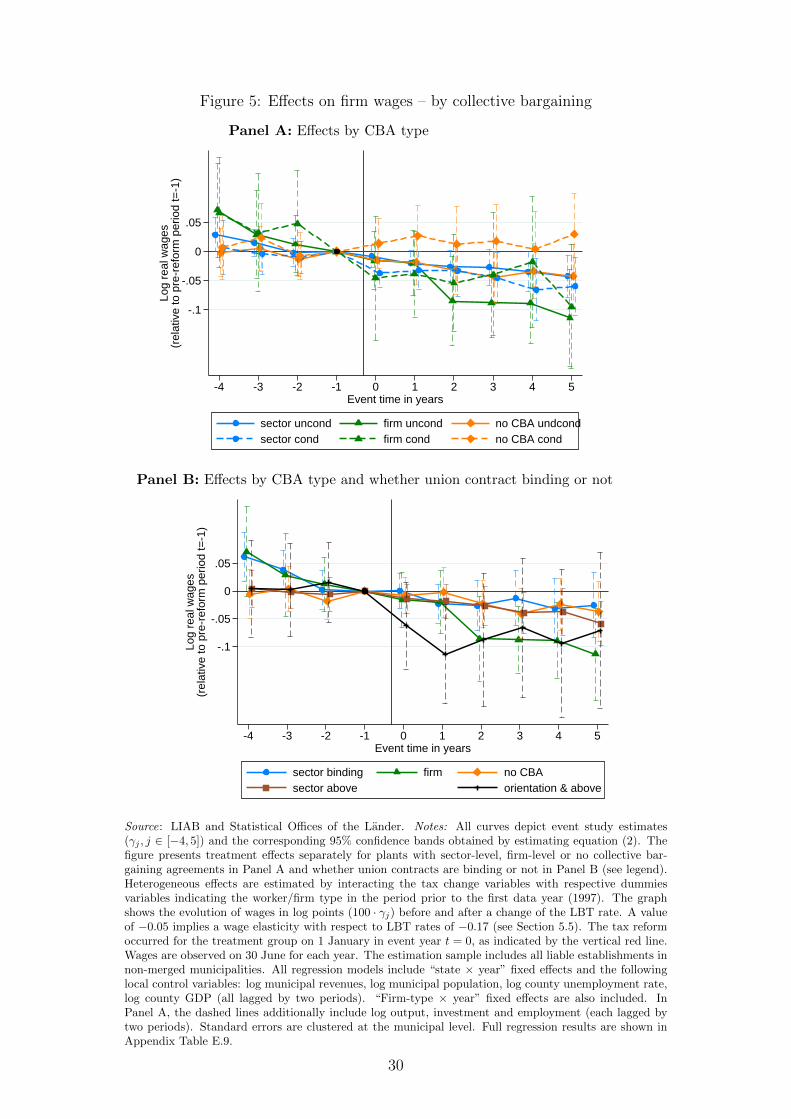
Figure 5: Effects on firm wages – by collective bargaining

Panel A: Effects by CBA type

-.1

-.05

0

.05

Log

real

wag

es(r

elat

ive

to p

re-r

efor

m p

erio

d t=

-1)

-4 -3 -2 -1 0 1 2 3 4 5Event time in years

sector uncond firm uncond no CBA undcondsector cond firm cond no CBA cond

Panel B: Effects by CBA type and whether union contract binding or not

-.1

-.05

0

.05

Log

real

wag

es(r

elat

ive

to p

re-r

efor

m p

erio

d t=

-1)

-4 -3 -2 -1 0 1 2 3 4 5Event time in years

sector binding firm no CBAsector above orientation & above

Source: LIAB and Statistical Offices of the Lander. Notes: All curves depict event study estimates(γj , j ∈ [−4, 5]) and the corresponding 95% confidence bands obtained by estimating equation (2). Thefigure presents treatment effects separately for plants with sector-level, firm-level or no collective bar-gaining agreements in Panel A and whether union contracts are binding or not in Panel B (see legend).Heterogeneous effects are estimated by interacting the tax change variables with respective dummiesvariables indicating the worker/firm type in the period prior to the first data year (1997). The graphshows the evolution of wages in log points (100 · γj) before and after a change of the LBT rate. A valueof −0.05 implies a wage elasticity with respect to LBT rates of −0.17 (see Section 5.5). The tax reformoccurred for the treatment group on 1 January in event year t = 0, as indicated by the vertical red line.Wages are observed on 30 June for each year. The estimation sample includes all liable establishments innon-merged municipalities. All regression models include “state × year” fixed effects and the followinglocal control variables: log municipal revenues, log municipal population, log county unemployment rate,log county GDP (all lagged by two periods). “Firm-type × year” fixed effects are also included. InPanel A, the dashed lines additionally include log output, investment and employment (each lagged bytwo periods). Standard errors are clustered at the municipal level. Full regression results are shown inAppendix Table E.9.

30

Theoretical Result 8 indicates that the wage effects of local business taxes are am-

biguous if firms operate plants in several jurisdictions. In fact, if we assume just one

type of labor, wage responses converges towards zero if the share of employment in the

taxed jurisdiction over total firm employment declines. Panel A of Figure 6 demonstrates

that we only find a negative effect for single-establishment firms, while establishments in

multi-plant firms show no significant wage response. It is possible that this effect is driven

by plant size as multi-establishment firms operate larger plants than single-establishment

firms. In Panel B of Figure 6, we interact the event study regressors with terciles of value

added in 199750 and test for differential size effect. We find that the largest plants do

not react significantly to changes in the business tax rate. But we do not find significant

size differences between single-plant and multi-plant firms. Our evidence thus supports

Result 8: formula apportionment can dilute the negative effect of taxes on wages. This

finding is also important for state-level corporate taxes in the U.S.

A possible explanation for the zero-wage effect for large firms could be that large

plants often belong to large, multinational companies. For these firms, tax-motivated

international profit shifting plays a role. As shown in Result 9, we expect wage effects to

be smaller in such multinational firms. Another mechanism to reduce the tax base is to

shift profits from labor income by, say, increasing wages of family members. This type of

adjustment, which may be particularly relevant for small firms, would also mitigate the

wage effect of corporate taxes. In view of the strongest effects for small firms depicted in

Panel B of Figure 6, we can reject the latter theoretical prediction empirically.

50 We find the same result when we (a) construct the size categories year by year and allow for switchingsize groups and (b) use number of employees as a measure of firm size

31

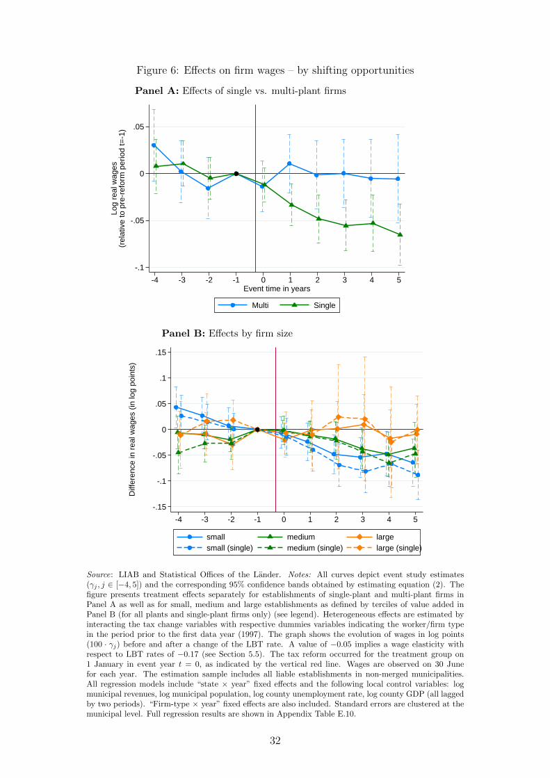
Figure 6: Effects on firm wages – by shifting opportunities

Panel A: Effects of single vs. multi-plant firms

-.1

-.05

0

.05

Log

real

wag

es(r

elat

ive

to p

re-r

efor

m p

erio

d t=

-1)

-4 -3 -2 -1 0 1 2 3 4 5Event time in years

Multi Single

Panel B: Effects by firm size

-.15

-.1

-.05

0

.05

.1

.15

Diff

eren

ce in

rea

l wag

es (

in lo

g po

ints

)

-4 -3 -2 -1 0 1 2 3 4 5

small medium largesmall (single) medium (single) large (single)

Source: LIAB and Statistical Offices of the Lander. Notes: All curves depict event study estimates(γj , j ∈ [−4, 5]) and the corresponding 95% confidence bands obtained by estimating equation (2). Thefigure presents treatment effects separately for establishments of single-plant and multi-plant firms inPanel A as well as for small, medium and large establishments as defined by terciles of value added inPanel B (for all plants and single-plant firms only) (see legend). Heterogeneous effects are estimated byinteracting the tax change variables with respective dummies variables indicating the worker/firm typein the period prior to the first data year (1997). The graph shows the evolution of wages in log points(100 · γj) before and after a change of the LBT rate. A value of −0.05 implies a wage elasticity withrespect to LBT rates of −0.17 (see Section 5.5). The tax reform occurred for the treatment group on1 January in event year t = 0, as indicated by the vertical red line. Wages are observed on 30 Junefor each year. The estimation sample includes all liable establishments in non-merged municipalities.All regression models include “state × year” fixed effects and the following local control variables: logmunicipal revenues, log municipal population, log county unemployment rate, log county GDP (all laggedby two periods). “Firm-type × year” fixed effects are also included. Standard errors are clustered at themunicipal level. Full regression results are shown in Appendix Table E.10.

32

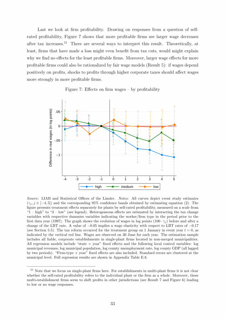
Last we look at firm profitability. Drawing on responses from a question of self-

rated profitability, Figure 7 shows that more profitable firms see larger wage decreases

after tax increases.51 There are several ways to interpret this result. Theoretically, at

least, firms that have made a loss might even benefit from tax cuts, would might explain

why we find no effects for the least profitable firms. Moreover, larger wage effects for more

profitable firms could also be rationalized by fair wage models (Result 5): if wages depend

positively on profits, shocks to profits through higher corporate taxes should affect wages

more strongly in more profitable firms.

Figure 7: Effects on firm wages – by profitability

-.1

-.05

0

.05

Diff

eren

ce in

rea

l wag

es (

in lo

g po

ints

)

-4 -3 -2 -1 0 1 2 3 4 5

high medium low

Source: LIAB and Statistical Offices of the Lander. Notes: All curves depict event study estimates(γj , j ∈ [−4, 5]) and the corresponding 95% confidence bands obtained by estimating equation (2). Thefigure presents treatment effects separately for plants by self-rated profitability, measured on a scale from“1 – high” to “3 – low” (see legend). Heterogeneous effects are estimated by interacting the tax changevariables with respective dummies variables indicating the worker/firm type in the period prior to thefirst data year (1997). The graph shows the evolution of wages in log points (100 · γj) before and after achange of the LBT rate. A value of −0.05 implies a wage elasticity with respect to LBT rates of −0.17(see Section 5.5). The tax reform occurred for the treatment group on 1 January in event year t = 0, asindicated by the vertical red line. Wages are observed on 30 June for each year. The estimation sampleincludes all liable, corporate establishments in single-plant firms located in non-merged municipalities.All regression models include “state × year” fixed effects and the following local control variables: logmunicipal revenues, log municipal population, log county unemployment rate, log county GDP (all laggedby two periods). “Firm-type × year” fixed effects are also included. Standard errors are clustered at themunicipal level. Full regression results are shown in Appendix Table E.8.

51 Note that we focus on single-plant firms here. For establishments in multi-plant firms it is not clearwhether the self-rated profitability refers to the individual plant or the firm as a whole. Moreover, thesemulti-establishment firms seem to shift profits in other jurisdictions (see Result 7 and Figure 6) leadingto low or no wage responses.

33

5.4 Heterogeneous worker effects

In this section, we test for worker heterogeneity by estimating model (3) at the individual

level.52 First, we verify the results obtained from the analysis at firm-level (see Appendix

Figures D.4). We then also restrict our estimation sample as above and focus on liable

firms in non-merged municipalities to test for heterogeneous worker effects.

In our first test, we look at the effect by skill level. Panel A of Figure 8 shows the

results. First, we consider the results when not accounting for wage censoring, that is,

when using the social security contribution (SSC) ceiling for censored individuals as the

observed wage. The solid lines show that medium-and low-skilled individuals show similar

negative wage responses. By contrast, we find no significant negative effect for high-skilled

workers. As discussed above, the finding for high-skilled might be biased towards zero as

wage responses for individuals above the SSC ceiling are not observed. Accordingly, we

re-estimate the model based on the sample of individuals who have never been censored

in their wages during the observation period. In this case, we find a very similar wage

effect across skill groups, as indicated by the dashed lines.

In Panel B of Figure 8, we differentiate by collar type. The graph shows that the

effect is stronger for blue-collar workers. A potential explanation for the difference is that

white-collar workers are relatively more mobile and hence see smaller wage responses to

tax rate changes.

52 Unlike the analysis at the firm-level, for which we used the median wage as our left-hand-side variable,the observed wage at the individual level might be problematic due to the censoring of the wages at theceiling for SSC. This might be particularly relevant for high-skilled workers. We address this issue below.

34

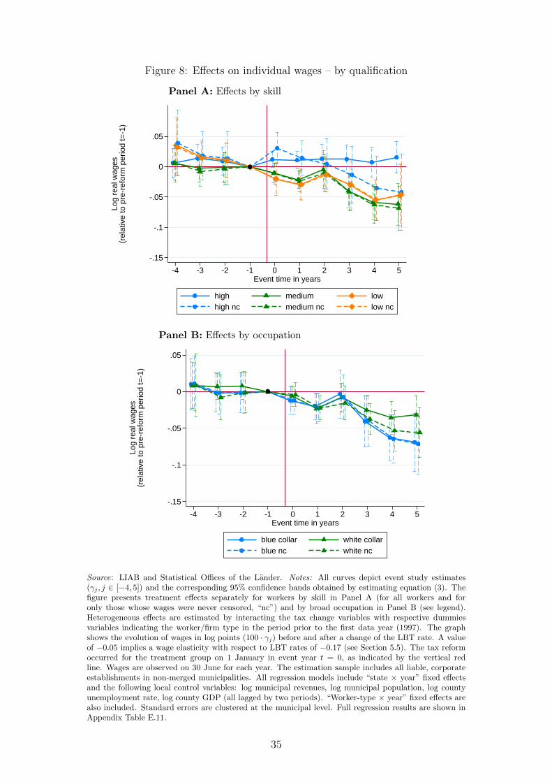
Figure 8: Effects on individual wages – by qualification

Panel A: Effects by skill

-.15

-.1

-.05

0

.05

Log

real

wag

es(r

elat

ive

to p

re-r

efor

m p

erio

d t=

-1)

-4 -3 -2 -1 0 1 2 3 4 5Event time in years

high medium lowhigh nc medium nc low nc

Panel B: Effects by occupation

-.15

-.1

-.05

0

.05

Log

real

wag

es(r

elat

ive

to p

re-r

efor

m p

erio

d t=

-1)

-4 -3 -2 -1 0 1 2 3 4 5Event time in years

blue collar white collarblue nc white nc

Source: LIAB and Statistical Offices of the Lander. Notes: All curves depict event study estimates(γj , j ∈ [−4, 5]) and the corresponding 95% confidence bands obtained by estimating equation (3). Thefigure presents treatment effects separately for workers by skill in Panel A (for all workers and foronly those whose wages were never censored, “nc”) and by broad occupation in Panel B (see legend).Heterogeneous effects are estimated by interacting the tax change variables with respective dummiesvariables indicating the worker/firm type in the period prior to the first data year (1997). The graphshows the evolution of wages in log points (100 · γj) before and after a change of the LBT rate. A valueof −0.05 implies a wage elasticity with respect to LBT rates of −0.17 (see Section 5.5). The tax reformoccurred for the treatment group on 1 January in event year t = 0, as indicated by the vertical redline. Wages are observed on 30 June for each year. The estimation sample includes all liable, corporateestablishments in non-merged municipalities. All regression models include “state × year” fixed effectsand the following local control variables: log municipal revenues, log municipal population, log countyunemployment rate, log county GDP (all lagged by two periods). “Worker-type × year” fixed effects arealso included. Standard errors are clustered at the municipal level. Full regression results are shown inAppendix Table E.11.

35

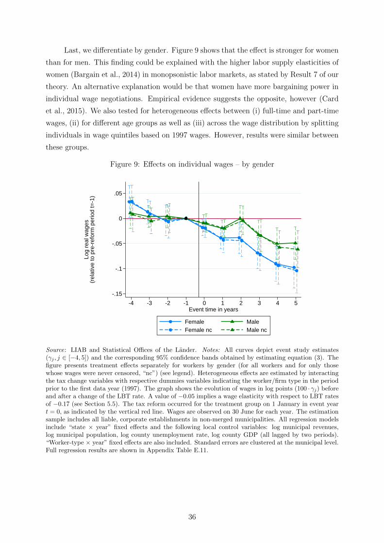
Last, we differentiate by gender. Figure 9 shows that the effect is stronger for women

than for men. This finding could be explained with the higher labor supply elasticities of

women (Bargain et al., 2014) in monopsonistic labor markets, as stated by Result 7 of our

theory. An alternative explanation would be that women have more bargaining power in

individual wage negotiations. Empirical evidence suggests the opposite, however (Card

et al., 2015). We also tested for heterogeneous effects between (i) full-time and part-time

wages, (ii) for different age groups as well as (iii) across the wage distribution by splitting

individuals in wage quintiles based on 1997 wages. However, results were similar between

these groups.

Figure 9: Effects on individual wages – by gender

-.15

-.1

-.05

0

.05

Log

real

wag

es(r

elat

ive

to p

re-r

efor

m p

erio

d t=

-1)

-4 -3 -2 -1 0 1 2 3 4 5Event time in years

Female MaleFemale nc Male nc

Source: LIAB and Statistical Offices of the Lander. Notes: All curves depict event study estimates(γj , j ∈ [−4, 5]) and the corresponding 95% confidence bands obtained by estimating equation (3). Thefigure presents treatment effects separately for workers by gender (for all workers and for only thosewhose wages were never censored, “nc”) (see legend). Heterogeneous effects are estimated by interactingthe tax change variables with respective dummies variables indicating the worker/firm type in the periodprior to the first data year (1997). The graph shows the evolution of wages in log points (100 · γj) beforeand after a change of the LBT rate. A value of −0.05 implies a wage elasticity with respect to LBT ratesof −0.17 (see Section 5.5). The tax reform occurred for the treatment group on 1 January in event yeart = 0, as indicated by the vertical red line. Wages are observed on 30 June for each year. The estimationsample includes all liable, corporate establishments in non-merged municipalities. All regression modelsinclude “state × year” fixed effects and the following local control variables: log municipal revenues,log municipal population, log county unemployment rate, log county GDP (all lagged by two periods).“Worker-type × year” fixed effects are also included. Standard errors are clustered at the municipal level.Full regression results are shown in Appendix Table E.11.

36

5.5 Measuring the tax incidence

In this subsection, we calculate what our wage elasticity estimates imply for the incidence

of the corporate tax on wages. In order to do this, we need to translate the wage responses

into money metrics. We follow Arulampalam et al. (2012) and calculate a measure that

describes the wage bill response to a marginal change in the tax bill, d(wL)d(τP )

. For given

production factors, it is straightforward to show that this measure is given by

d(wL)

d(τP )=

Ldw

Pdτ + τdP=

Ldw

Pdτ − τLdw= 1/

(1

ηwLτP

− τ

),

where η is the wage elasticity with respect to the tax rate. The measure d(wL)d(τP )

describes

how much of a marginal change in tax liabilities is borne by workers through lower wages.

Note that the total tax burden is likely to be higher than tax liabilities due to the marginal

excess burden of taxation, MEB. In this case, the share of workers in the overall burden

of a corporate tax change is given by d(wL)d(τP )

· 1(1+MEB)

.

Table 1 shows our results for the wage effects after five years. Our preferred estimate

(liable firms in non-merged municipalities) is equal to −0.00047, which corresponds to a

wage elasticities of −0.142. This estimates implies that a 1-euro increase in a firm’s tax

bill leads to a decrease in the wage bill of 56 cents. As we cannot estimate the marginal

excess burden with the data at hand, we have to rely on estimates from the literature

to quantify the total incidence on labor. If we assume a marginal deadweight loss of

corporate taxation of 29% as suggested by Devereux et al. (2014), 43% of the total tax

burden is borne by workers. This finding is comparable to other studies analyzing the

corporate tax incidence on wages (Arulampalam et al., 2012; Liu and Altshuler, 2013;

Suarez Serrato and Zidar, 2014). While the former two studies find that the a 1-dollar

increase in the tax bill leads to a 50-cent decrease in the wage bill (not accounting for the

marginal excess burden), the latter study finds that worker bear 30-35% of the total tax

burden.

Table 1 further reports wage elasticities and money metrics for different samples

and firm types. While incidence measures are similar for manufacturing and service

sector firms, we find differences with respect to collective bargaining agreements. Our

results show that responses in firms with firm-level bargaining are much higher than in

firms with sector-level CBAs. In fact, wage responses in firms where bargaining takes

place at the sector-level are similar to responses in firms without a CBA, which suggests

that business taxes also interact with other wage setting institutions.

37

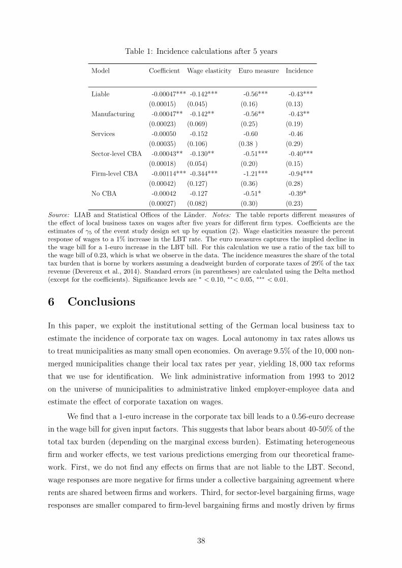
Table 1: Incidence calculations after 5 years

Model Coefficient Wage elasticity Euro measure Incidence

Liable -0.00047*** -0.142*** -0.56*** -0.43***

(0.00015) (0.045) (0.16) (0.13)

Manufacturing -0.00047** -0.142** -0.56** -0.43**

(0.00023) (0.069) (0.25) (0.19)

Services -0.00050 -0.152 -0.60 -0.46

(0.00035) (0.106) (0.38 ) (0.29)

Sector-level CBA -0.00043** -0.130** -0.51*** -0.40***

(0.00018) (0.054) (0.20) (0.15)

Firm-level CBA -0.00114*** -0.344*** -1.21*** -0.94***

(0.00042) (0.127) (0.36) (0.28)

No CBA -0.00042 -0.127 -0.51* -0.39*

(0.00027) (0.082) (0.30) (0.23)

Source: LIAB and Statistical Offices of the Lander. Notes: The table reports different measures ofthe effect of local business taxes on wages after five years for different firm types. Coefficients are theestimates of γ5 of the event study design set up by equation (2). Wage elasticities measure the percentresponse of wages to a 1% increase in the LBT rate. The euro measures captures the implied decline inthe wage bill for a 1-euro increase in the LBT bill. For this calculation we use a ratio of the tax bill tothe wage bill of 0.23, which is what we observe in the data. The incidence measures the share of the totaltax burden that is borne by workers assuming a deadweight burden of corporate taxes of 29% of the taxrevenue (Devereux et al., 2014). Standard errors (in parentheses) are calculated using the Delta method(except for the coefficients). Significance levels are ∗ < 0.10, ∗∗< 0.05, ∗∗∗ < 0.01.

6 Conclusions

In this paper, we exploit the institutional setting of the German local business tax to

estimate the incidence of corporate tax on wages. Local autonomy in tax rates allows us

to treat municipalities as many small open economies. On average 9.5% of the 10, 000 non-

merged municipalities change their local tax rates per year, yielding 18, 000 tax reforms

that we use for identification. We link administrative information from 1993 to 2012

on the universe of municipalities to administrative linked employer-employee data and

estimate the effect of corporate taxation on wages.

We find that a 1-euro increase in the corporate tax bill leads to a 0.56-euro decrease

in the wage bill for given input factors. This suggests that labor bears about 40-50% of the

total tax burden (depending on the marginal excess burden). Estimating heterogeneous

firm and worker effects, we test various predictions emerging from our theoretical frame-

work. First, we do not find any effects on firms that are not liable to the LBT. Second,

wage responses are more negative for firms under a collective bargaining agreement where

rents are shared between firms and workers. Third, for sector-level bargaining firms, wage

responses are smaller compared to firm-level bargaining firms and mostly driven by firms

38

that pay wages above the collective bargaining contract. Fourth, firms without collec-

tive bargaining agreements only show a negative wage response if they follow sector-level

union contracts, which could be rationalized with fair wage models. Fifth, wage effects

are close to zero for firms which operate in multiple jurisdictions. This can be explained

by formula apportionment and profit shifting opportunities across municipalities. Sixth,

we find smaller effects for larger plants, which are more likely to be part of a multina-

tional groups, and hence may exploit international profit shifting opportunities leading to

smaller wage effects.

Several general lessons can be learned from our analysis. First, we confirm most

economists’ beliefs and theoretical predictions that labor bares a substantial share of the

corporate tax burden. Our estimates suggests that roughly 40% of the tax burden is

passed onto workers. Importantly, this finding is obtained by exploiting variation at the

municipal level, which may have implications for the size of the estimate. Compared to

changes in national corporate tax rates, two potential differences are worth noting. On

the one hand, labor is likely to be more mobile compared with capital at the local level,

which attenuates the wage effect. On the other hand, focusing on tax changes at the local

level implies that price changes (both of goods and other production factors) are probably

much smaller than in the case of national corporate tax changes. This would imply that

wage effects of local tax changes are larger.

Second, our theoretical predictions and empirical findings strongly suggests that

labor market institutions be considered when assessing the incidence of corporate taxes

on wages. If there are rents in the labor market, due, say, to collective bargaining or firms

with monopsonistic power, there are direct effects on wages in addition to conventional

effects induced by adjustments in production factors. Moreover, national or international

profit-shifting possibilities attenuate the negative effect of corporate taxation on wages.

Last, in terms of policy implications, our analysis suggests that it is worth taking

distributional effects into account. We find that part of the tax burden is borne by low-

skilled workers. While our results do not suggest that high-skilled workers bear a smaller

part of the corporate tax burden, the view that the corporate income tax primarily falls

on firm owners is rejected by our analysis. At the same time we find that a larger part

of the corporate tax is borne by employees capturing rents in the labor market. The fact

that employees in competitive segments of labor markets, where wages are lower, bear a

smaller part of the corporate tax burden may be seen as a desirable feature of the tax.

39

References

Acemoglu, D. and R. Shimer (1999). Efficient Unemployment Insurance. Journal of

Political Economy 107 (5), 893–928.

Akerlof, G. A. and J. L. Yellen (1990). The Fair Wage-Effort Hypothesis and Unemploy-

ment. The Quarterly Journal of Economics 105 (2), 255–283.

Alda, H., S. Bender, and H. Gartner (2005). European Data Watch: The Linked

Employer-Employee Dataset Created from the IAB Establishment Panel and the

Process-Produced data of the IAB (LIAB). Schmollers Jahrbuch: Journal of Applied

Social Science Studies 125 (2), 327–336.

Amiti, M. and D. R. Davis (2010). Trade, Firms, and Wages: Theory and Evidence.

Review of Economic Studies 79 (1), 1–36.

Andrews, M., T. Schank, and R. Upward (2006). Practical fixed-effects estimation meth-

ods for the three-way error-components model. Stata Journal 6 (4), 461–481.

Angrist, J. D. and J.-S. Pischke (2009). Mostly Harmless Econometrics. Princeton, New

Jersey: Princeton University Press.

Arulampalam, W., M. P. Devereux, and G. Maffini (2012). The Direct Incidence of

Corporate Income Tax on Wages. European Economc Review 56 (6), 1038–1054.

Auerbach, A. J. (2005). Who Bears the Corporate Tax? A Review of What We Know.

NBER Working Paper No. 11686.

Ballentine, J. G. (1978). The Incidence of a Corporation Income Tax in a Growing

Economy. Journal of Political Economy 86 (5), 863–875.

Bargain, O., A. Peichl, and K. Orsini (2014). Comparing Labor Supply Elasticities in

Europe and the US: New Results. Journal of Human Resources 49 (3), 723–838.

Barth, E. and J. Zweimuller (1995). Relative Wages under Decentralized and Corporatist

Bargaining Systems. Scandinavian Journal of Economics 97 (3), 369–384.

Bauer, T. K., T. Kasten, and L. Siemers (2012). Business taxation and wages: Evidence

from individual panel data. IZA Discussion Paper No. 6717.

Bender, S., A. Haas, and C. Klose (2000). The IAB Employment Subsample 1975-1995.

Schmollers Jahrbuch: Journal of Applied Social Science Studies 120 (4), 649–662.

40

Bertrand, M., E. Duflo, and S. Mullainathan (2004). How Much Should we Trust

Difference-in-Difference Estimates? Quarterly Journal of Economics 119 (1), 249–275.

Bird, R. M. (2003). A new look at local business taxes. Tax Notes International 30,

695–711.

Boeri, T. (2014). Two-Tier Bargaining. IZA Discussion Paper No. 8358.

Bradford, D. F. (1978). Factor prices may be constant but factor returns are not. Eco-

nomics Letters 1 (3), 199–203.

Buttner, T. (2003). Tax Base Effects and Fiscal Externalities of Local Capital Taxation:

Evidence from a Panel of German Jurisdictions. Journal of Urban Economics 54 (1),

110–128.

Card, D., A. R. Cardoso, and P. Kline (2015). Bargaining, Sorting, and the Gender Wage

Gap: Quantifying the Impact of Firms on the Relative Pay of Women. The Quarterly

Journal of Economics doi: 10.1093/qje/qjv038.

Card, D., J. Heining, and P. Kline (2013). Workplace heterogeneity and the rise of west

german wage inequality. The Quarterly Journal of Economics .

Castanheira, M., G. Nicodeme, and P. Profeta (2012). On the political economics of tax

reforms: survey and empirical assessment. International Tax and Public Finance 19,

598–624.

Desai, M. A., C. F. Foley, and J. R. Hines (2007). Labor and Capital Shares of the

Corporate Tax Burden: International Evidence. mimeo, presented at the International

Tax Policy Forum and Urban-Brookings Tax Policy Center conference on Who Pays

the Corporate Tax in an Open Economy?, 18 December, 2007.

Devereux, M., L. Liu, and S. Loretz (2014). The Elasticity of Corporate Taxable In-

come: New Evidence from UK Tax Records. American Economic Journal: Economic

Policy 6 (2), 19–53.

Diamond, P. A. and J. Mirrlees (1971). Optimal Taxation and Public Production. Amer-

ican Economic Review 61, 8–27 and 261–278.

Du Caju, P., E. Gautier, D. Momferatou, and M. Ward-Warmedinger (2008). Institutional

features of wage bargaining in 23 european countries, the us and japan,. ECB Working

Paper Series No 974.

41

Dustmann, C., B. Fitzenberger, U. Schonberg, and A. Spitz-Oehner (2014). From sick man

of europe to economic superstar: Germany’s resurgent economy. Journal of Economic

Perspectives 28 (1), 167–188.

Dustmann, C., J. Ludsteck, and U. Schoenberg (2009). Revisiting the german wage

structure. Quarterly Journal of Economics 124 (2), 843–881.

Dwenger, N., P. Rattenhuber, and V. Steiner (2011). Sharing the burden: Empirical

evidence of corporate tax incidence. Preprint of the Max Planck Institute for Tax Law

and Public Finance 2011-14.

Egger, H. and U. Kreickemeier (2012). Fairness, trade, and inequality. Journal of Inter-

national Economics 86 (2), 184–196.

Ellguth, P., H.-D. Gerner, and J. Stegmaier (2012). Wage Bargaining in Germany – the

Role of Works Councils and Opening Clauses. IAB Discussion Paper 05/2012.

Feldstein, M. (1974). Incidence of a Capital Income Tax in a Growing Economy with

Variable Savings Rates. The Review of Economic Studies 41 (4), 505–513.

Felix, R. A. (2007). Passing the Burden: Corporate Tax Incidence in Open Economies.

Federal Reserve Bank of Kansas City Regional Research Working Paper 07-01.

Felix, R. A. and J. R. Hines (2009). Corporate Taxes and Union Wages in the United

States. NBER Working Paper No. 15263.

Foremny, D. and N. Riedel (2014). Business Taxes and the Electoral Cycle. Journal of

Public Economics .

Fuchs, V. R., A. B. Krueger, and J. M. Poterba (1998). Economists’ views about param-

eters, values, and policies: Survey results in labor and public economics. Journal of

Economic Literature 36 (3), 1387–1425.

Fuest, C., A. Peichl, and S. Siegloch (2011). Do Employees Bear the Burden of Corporate

Taxation? A Micro Level Approach Using Linked Employer-Employee Data. Presented

at the 67th Annual Congress of the International Institute of Public Finance in Ann

Arbor.

Fuest, C., A. Peichl, and S. Siegloch (2013). Do Higher Corporate Taxes Reduce Wages?

Micro Evidence from Germany. IZA Discussion Paper No. 7390.

Gravelle, J. C. (2013). Corporate Tax Incidence: Review of General Equilibirum Estimates

and Analysis. National Tax Journal 66 (1), 185–214.

42

Harberger, A. C. (1962). The incidence of the corporation income tax. Journal of Political

Economy 70, 215–240.

Harberger, A. C. (1995). The ABCs of Corporate Tax Incidence: Insights into the Open-

Economy Case. In Tax Policy and Economic Growth: Proceedings of a Symposium

sponsored by the American Council for Capital Formation, pp. 51–73. Washington:

ACCF Center for Policy Research.

Harberger, A. C. (2006). Corporate Tax Incidence: Reflections on What Is Known,

Unknonw and Unknowable. In J. W. Diamond and G. R. Zodrow (Eds.), Fundamental

Tax Reforms: Issues, Choices, and Implications, pp. 283–308. Cambridge, MA: MIT

Press.

Hassett, K. A. and A. Mathur (2006). Taxes and Wages. AEI Working Paper No. 128.

Janeba, E. and S. Osterloh (2012). Tax and the city: A theory of local tax competition

and evidence for Germany. ZEW Discussion Papers No. 12-005.

Kawano, L. and J. Slemrod (2012). The Effect of Tax Rates and Tax Bases on Corporate

Tax Revenues: Estimates with New Measures of the Corporate Tax Base. NBER

Working Papers 18440.

Kolling, A. (2000). The IAB-Establishment Panel. Schmollers Jahrbuch: Journal of

Applied Social Science Studies 120 (2), 291–300.

Kotlikoff, L. J. and L. H. Summers (1987). Tax Incidence. In A. J. Auerbach and M. Feld-

stein (Eds.), Handbook of Public Economics, Volume 2, pp. 1043–1092. Amsterdam:

Elsevier.

Liu, L. and R. Altshuler (2013). Measuring the burden of the corporate income tax under

imperfect competition. National Tax Journal 66 (1), 215–237.

McDonald, I. M. and R. E. Solow (1981). Wage Bargaining and Employment. The

America Economic Review 71 (5), 896–908.

NCSL (2009). State, federal and local taxes. http://www.ncsl.org/documents/fiscal/

statefederalandlocaltaxes.pdf.

OECD (2015). Tax on corporate profits (indicator). doi: 10.1787/d30cc412-en.

Oswald, A. J. (1993). Efficient contracts are on the labour demand curve: Theory and

facts. Labour Economics 1 (1), 85–113.

43

Ratti, R. A. and P. Shome (1977). On a General Equilibrium Model of the Incidence of

the Corporation Tax under Uncertainty. Journal of Public Economics 8 (2), 233–238.

Rogerson, R., R. Shimer, and R. Wright (2005). Search-Theoretic Models of the Labor

Market: A Survey. Journal of Economic Literature 43 (4), 959–988.

Sandler, D. H. and R. Sandler (2014). Multiple event studies in public finance and labor

economics: A simulation study with applications. Journal of Economic and Social

Measurement 39, 31–57.

Shapiro, C. and J. Stiglitz (1984). Equilibrium unemployment as a worker discipline

device. The American Economic Review 74, 433–444.

Shoven, J. B. (1976). The Incidence and Efficiency Effects of Taxes on Income from

Capital. Journal of Political Economy 84 (6), 1261–1283.

Siegloch, S. (2013). Employment Effects of Local Corporate Taxes. Mimeo.

Solow, R. M. (1979). Another possible source of wage stickiness. Journal of Macroeco-

nomics 1 (1), 79–82.

Spengel, C., D. Endres, K. Finke, and J. H. Heckemeyer (2014). Effective Tax

Levels using the Devereux/Griffith Methodology. Project for the EU Commission

TAXUD/2013/CC/120 Final Report.

Suarez Serrato, J. C. and O. Zidar (2014). Who Benefits from State Corporate Tax Cuts?

A Local Labor Markets Approach with Heterogeneous Firms. NBER Working Paper

20289.

44

Appendices for online publication only

A Theoretical derivations

In this appendix, we discuss the implications of various wage setting models for the impact

of corporate tax changes on wages. We do so by using the model introduced in the main

text, which we discuss here in greater detail. As will be explained further below, the

model will be varied slightly to incorporate different assumptions about wage setting and

two aspects of the tax system relating to formula apportionment and income shifting.

Consider an economy which consists of n jurisdictions. There are firms in the econ-

omy. To ease notation we normalize the number of firms per jurisdiction to unity. Firms

use the following factors of production: capital (K) and labor of two skill levels. Labor of

skill type k, k = h, l, is denoted by Lk. We will consider different production technologies.

In the base version of the model we consider a production function F (K,Lh, Ll), which is

assumed to have the usual neoclassical properties and to exhibit declining returns to scale.

One interpretation is that there is an implicit fourth factor which may be interpreted as a

location specific rent. While capital and both types of labor are mobile across municipal

borders, firms are immobile, due to the location specific rent.

The after-tax profit of a firm i located in jurisdiction j , j = 1...n, is given by

Pij = piFi(Ki, Lhi , L

li)(1− τj)−

∑k

wki Lki (1− φτj)− (1− ατj)rKi (4)

where pi is the output price, wki is the wage for labor of skill type k, τj is the corporate

income tax rate of jurisdiction j and r is the non-tax cost of capital. The variables φ, α

are tax base parameters representing the shares of the wage and capital costs, which can

be deducted from the tax base. These parameters are the same in all jurisdictions. We

assume 0 ≤ φ ≤ 1, 0 ≤ α ≤ 1. Since there is only one firm per jurisdiction, we can drop

the subscript j. We also normalize the output price to unity.

In some variants of the model labor markets may not be clear. In these cases, we

assume that unemployed workers of skill type k receive unemployment benefits denoted

by wk.

A.1 Competitive labor market

Assume that input and output markets are perfectly competitive, so that factor prices

will adjust to equate demand and supply. Factor demand functions are given by the firm’s

first order conditions

45

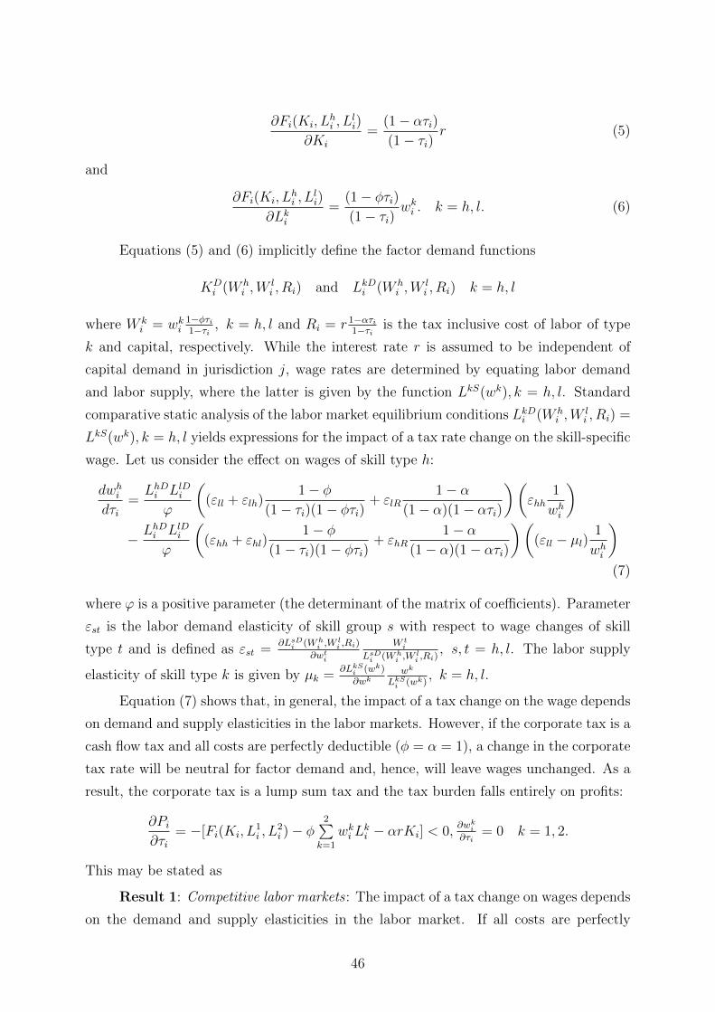
∂Fi(Ki, Lhi , L

li)

∂Ki

=(1− ατi)(1− τi)

r (5)

and

∂Fi(Ki, Lhi , L

li)

∂Lki=

(1− φτi)(1− τi)

wki . k = h, l. (6)

Equations (5) and (6) implicitly define the factor demand functions

KDi (W h

i ,Wli , Ri) and LkDi (W h

i ,Wli , Ri) k = h, l

where W ki = wki

1−φτi1−τi , k = h, l and Ri = r 1−ατi

1−τi is the tax inclusive cost of labor of type

k and capital, respectively. While the interest rate r is assumed to be independent of

capital demand in jurisdiction j, wage rates are determined by equating labor demand

and labor supply, where the latter is given by the function LkS(wk), k = h, l. Standard

comparative static analysis of the labor market equilibrium conditions LkDi (W hi ,W

li , Ri) =

LkS(wk), k = h, l yields expressions for the impact of a tax rate change on the skill-specific

wage. Let us consider the effect on wages of skill type h:

dwhidτi

=LhDi LlDi

ϕ

((εll + εlh)

1− φ(1− τi)(1− φτi)

+ εlR1− α

(1− α)(1− ατi)

)(εhh

1

whi

)− LhDi LlDi

ϕ

((εhh + εhl)

1− φ(1− τi)(1− φτi)

+ εhR1− α

(1− α)(1− ατi)

)((εll − µl)

1

whi

)(7)

where ϕ is a positive parameter (the determinant of the matrix of coefficients). Parameter

εst is the labor demand elasticity of skill group s with respect to wage changes of skill

type t and is defined as εst =∂LsD

i (Whi ,W

li ,Ri)

∂wti

W ti

LsDi (Wh

i ,Wli ,Ri)

, s, t = h, l. The labor supply

elasticity of skill type k is given by µk =∂LkS

i (wk)

∂wkwk

LkSi (wk)

, k = h, l.

Equation (7) shows that, in general, the impact of a tax change on the wage depends

on demand and supply elasticities in the labor markets. However, if the corporate tax is a

cash flow tax and all costs are perfectly deductible (φ = α = 1), a change in the corporate

tax rate will be neutral for factor demand and, hence, will leave wages unchanged. As a

result, the corporate tax is a lump sum tax and the tax burden falls entirely on profits:

∂Pi∂τi

= −[Fi(Ki, L1i , L

2i )− φ

2∑k=1

wki Lki − αrKi] < 0,

∂wki

∂τi= 0 k = 1, 2.

This may be stated as

Result 1: Competitive labor markets : The impact of a tax change on wages depends

on the demand and supply elasticities in the labor market. If all costs are perfectly

46

deductible, the burden of the corporate income tax is fully borne by firm owners. Then a

tax rate change does not affect the wage rate.

A.2 Corporate tax incidence with wage bargaining

A.2.1 Individual wage bargaining

We now assume that wages are determined by bargaining between firms and individual

workers. The output a worker of type k generates in firm i is given by Qki (K

ki ) and the

additional profit the firm earns is Qki (K

ki )(1−τi)−wki (1−φτi)−(1−ατi)rKk

i . The variable

Kki is the capital the firm invests to equip the worker. The outcome of the bargaining

process is given by

wk∗i = arg maxwk

i

Ωi

where

Ωi = βki ln(wki − wk) + (1− βki ) lnPi.

The variable βki ∈ (0, 1) stands for the relative bargaining power of the employee. The

first order conditions of the bargaining problem yield

wk∗i = (1− βki )wk + βkiQki (K

ki )(1− τi)− (1− ατi)rKk

i

(1− φτi). (8)

The effect of a change in the corporate tax rate on the wage is

∂wk∗i∂τi

= −βki(Qk

i (Kki )− rKk

i )(1− φ) + (1− α)rKki

(1− φτi)2≤ 0. (9)

A higher corporate tax reduces the wage unless both wage and capital costs are fully

deductible. This may be stated as

Result 2: Individual wage bargaining : If wage or capital costs are less than fully

deductible, an increase (decline) in the local corporate tax rate reduces (increases) the

wage. The effect increases with the relative bargaining power of the employee.

A.2.2 Collective wage bargaining

Assume that workers are represented by trade unions. We consider two cases: The first

case is firm-level bargaining, where firm-level unions bargain with individual firms. The

second case is sector-level bargaining, where sector-level unions bargain with sector-level

employer organizations.

47

Firm-level bargaining. Denote the wage for a worker of skill type k employed by a

firm located in jurisdiction i by wki = wki +ski , where ski is the wage premium generated by

bargaining at the firm-level. The bargaining model we use for the firm-level is a standard

efficient bargaining model (McDonald and Solow, 1981), where unions and firms bargain

over the wage premium, ski , and employment Lki . Each skill type is represented by one

trade union and each firm negotiates with the two unions simultaneously (Barth and

Zweimuller, 1995). The objective function of the trade union representing the workers of

skill type k in firm i is given by

Zki = Lki (w

ki − wk) = Lki s

ki .

In the case of disagreement, the rent of the union Zki and the firm’s profit Pi are equal

to zero. After wages and employment levels are determined, firms set Ki to maximize

profits:

∂F (Ki, Lhi , L

li)

∂Ki

= Ri (10)

where Ri denotes the cost of capital:

Ri = r(1− ατi)(1− τi)

.

The outcome of the bargaining process is given by

sk∗i , Lk∗i = arg max

ski ,Lki

Ωki

where

Ωki = βki lnZk

i + (1− βki ) lnPi.

The variable βki ∈ (0, 1) stands for relative bargaining power of the skill type k union in

firm i. The first order conditions of the bargaining problem yield

sk∗i =(1− βji )βki(1− βki β

ji )

Πi

Lki (1− φτi)k, j = h, l, k 6= j (11)

where

Πi = F (Ki, Lhi , L

li)(1− τi)−

∑k w

kLki (1− φτi)− (1− ατi)rKi.

48

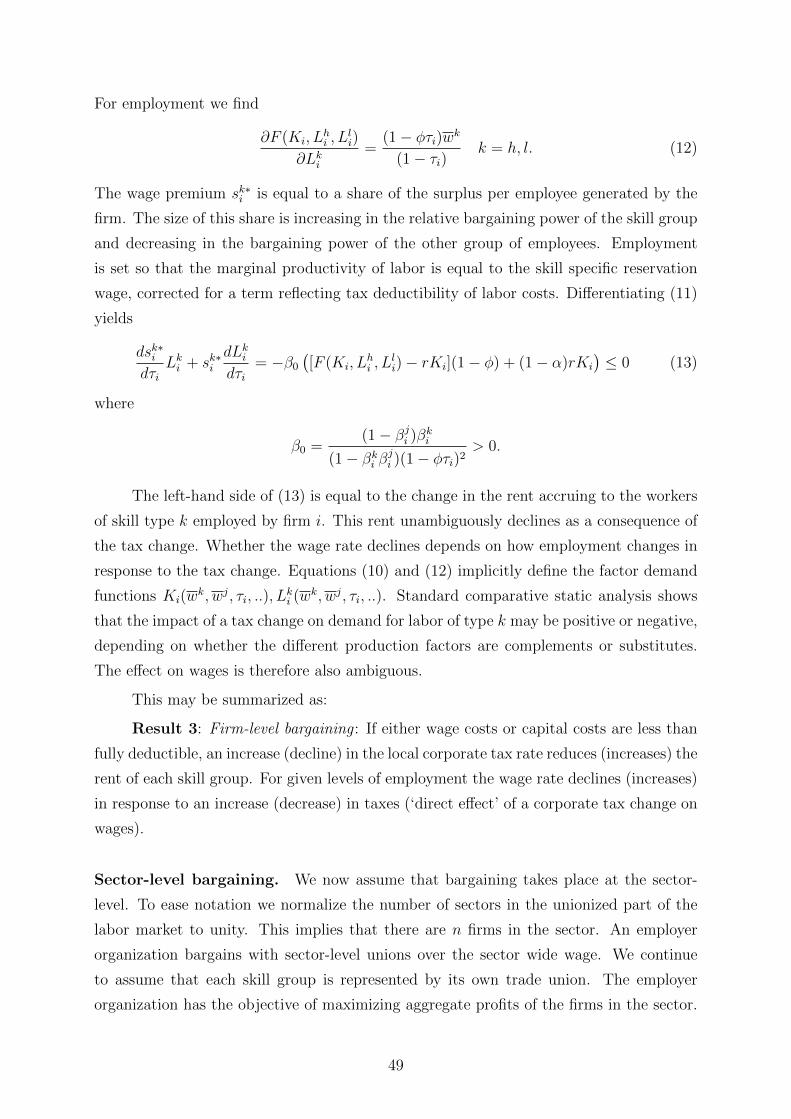
For employment we find

∂F (Ki, Lhi , L

li)

∂Lki=

(1− φτi)wk

(1− τi)k = h, l. (12)

The wage premium sk∗i is equal to a share of the surplus per employee generated by the

firm. The size of this share is increasing in the relative bargaining power of the skill group

and decreasing in the bargaining power of the other group of employees. Employment

is set so that the marginal productivity of labor is equal to the skill specific reservation

wage, corrected for a term reflecting tax deductibility of labor costs. Differentiating (11)

yields

dsk∗idτi

Lki + sk∗idLkidτi

= −β0([F (Ki, L

hi , L

li)− rKi](1− φ) + (1− α)rKi

)≤ 0 (13)

where

β0 =(1− βji )βki

(1− βki βji )(1− φτi)2

> 0.

The left-hand side of (13) is equal to the change in the rent accruing to the workers

of skill type k employed by firm i. This rent unambiguously declines as a consequence of

the tax change. Whether the wage rate declines depends on how employment changes in

response to the tax change. Equations (10) and (12) implicitly define the factor demand

functions Ki(wk, wj, τi, ..), L

ki (w

k, wj, τi, ..). Standard comparative static analysis shows

that the impact of a tax change on demand for labor of type k may be positive or negative,

depending on whether the different production factors are complements or substitutes.

The effect on wages is therefore also ambiguous.

This may be summarized as:

Result 3: Firm-level bargaining : If either wage costs or capital costs are less than

fully deductible, an increase (decline) in the local corporate tax rate reduces (increases) the

rent of each skill group. For given levels of employment the wage rate declines (increases)

in response to an increase (decrease) in taxes (‘direct effect’ of a corporate tax change on

wages).

Sector-level bargaining. We now assume that bargaining takes place at the sector-

level. To ease notation we normalize the number of sectors in the unionized part of the

labor market to unity. This implies that there are n firms in the sector. An employer

organization bargains with sector-level unions over the sector wide wage. We continue

to assume that each skill group is represented by its own trade union. The employer

organization has the objective of maximizing aggregate profits of the firms in the sector.

49

Following the seniority model proposed by Oswald (1993), we assume that each union

wishes to maximize the premium over the reservation wage for the skill group it represents,

which is given by vk = wk−wk. For given wages, firms set profit maximizing employment.

The outcome of the sector-level bargaining process is given by

vk∗ = arg maxpk

ΩSki

where

ΩSki = γk ln vk + (1− γk) ln

m∑i=1

Pi.

The variable γk ∈ (0, 1) stands for the relative bargaining power of the sector-level skill

type k union. Rearranging the first order condition of the bargaining problem yields

vk∗ = γ0

n∑i=1

Πi

n∑i=1

Lki (1− φτi)k, j = h, l, k 6= j (14)

where

γ0 =(1− γj)γk

(1− γjγk)> 0.

The sector wide wage premium is equal to a share of the average surplus per worker

generated by the firms in the sector. Employment and investment decisions are now given

by

∂F (Ki, Lhi , L

li)

∂Lki=

(1− φτi)wk

(1− τi)k = h, l (15)

and

∂F (Ki, Lhi , L

li)

∂Ki

= Ri.

How does a corporate tax change in jurisdiction m , m ∈ (1, ..., n), affect vk∗? Total

differentiation of equation (14) yields

50

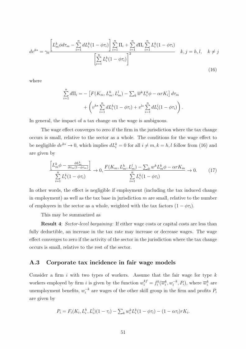
dvk∗ = γ0

[Lkmφdτm −

n∑i=1

dLki (1− φτi)]

n∑i=1

Πi +n∑i=1

dΠi

n∑i=1

Lki (1− φτi)[n∑i=1

Lki (1− φτi)]2 k, j = h, l, k 6= j

(16)

where

n∑i=1

dΠi =−[F (Km, L

hm, L

lm)−

∑k w

kLki φ− αrKi

]dτm

+

(vh∗

n∑i=1

dLhi (1− φτi) + vl∗n∑i=1

dLli(1− φτi)).

In general, the impact of a tax change on the wage is ambiguous.

The wage effect converges to zero if the firm in the jurisdiction where the tax change

occurs is small, relative to the sector as a whole. The conditions for the wage effect to

be negligible dvk∗ → 0, which implies dLki = 0 for all i 6= m, k = h, l follow from (16) and

are given by[Lkmφ−

∂Lkm

∂τm(1−φτm)

]n∑i=1

Lki (1− φτi)→ 0,

F (Km, Lhm, L

lm)−

∑k w

kLkmφ− αrKmn∑i=1

Lki (1− φτi)→ 0. (17)

In other words, the effect is negligible if employment (including the tax induced change

in employment) as well as the tax base in jurisdiction m are small, relative to the number

of employees in the sector as a whole, weighted with the tax factors (1− φτi).

This may be summarized as

Result 4: Sector-level bargaining : If either wage costs or capital costs are less than

fully deductible, an increase in the tax rate may increase or decrease wages. The wage

effect converges to zero if the activity of the sector in the jurisdiction where the tax change

occurs is small, relative to the rest of the sector.

A.3 Corporate tax incidence in fair wage models

Consider a firm i with two types of workers. Assume that the fair wage for type k

workers employed by firm i is given by the function wkfi = fki (wki , w−ki , Pi), where wki are

unemployment benefits, w−ki are wages of the other skill group in the firm and profits Pi

are given by

Pi = Fi(Ki, Lhi , L

li)(1− τi)−

∑k w

ki L

ki (1− φτi)− (1− ατi)rKi.

51

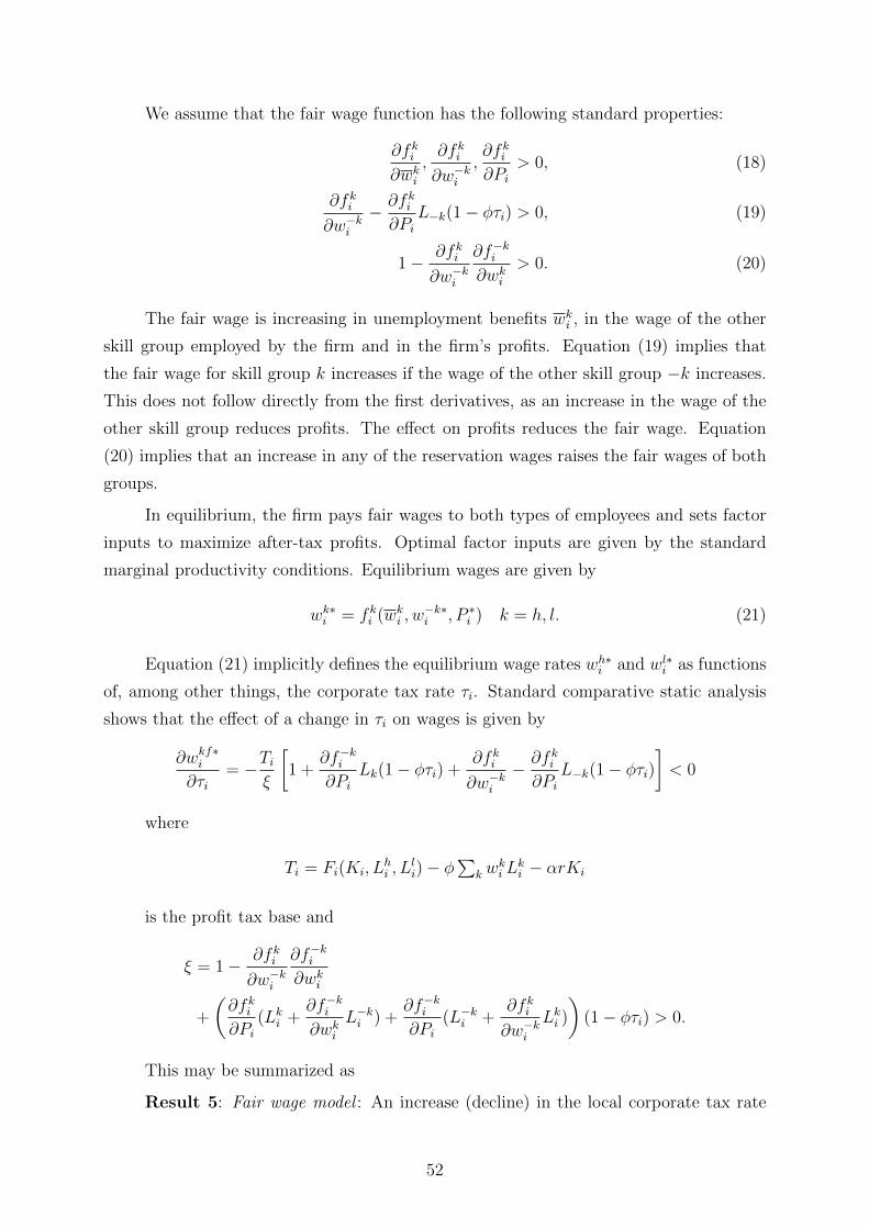
We assume that the fair wage function has the following standard properties:

∂fki∂wki

,∂fki∂w−ki

,∂fki∂Pi

> 0, (18)

∂fki∂w−ki

− ∂fki∂Pi

L−k(1− φτi) > 0, (19)

1− ∂fki∂w−ki

∂f−ki∂wki

> 0. (20)

The fair wage is increasing in unemployment benefits wki , in the wage of the other

skill group employed by the firm and in the firm’s profits. Equation (19) implies that

the fair wage for skill group k increases if the wage of the other skill group −k increases.

This does not follow directly from the first derivatives, as an increase in the wage of the

other skill group reduces profits. The effect on profits reduces the fair wage. Equation

(20) implies that an increase in any of the reservation wages raises the fair wages of both

groups.

In equilibrium, the firm pays fair wages to both types of employees and sets factor

inputs to maximize after-tax profits. Optimal factor inputs are given by the standard

marginal productivity conditions. Equilibrium wages are given by

wk∗i = fki (wki , w−k∗i , P ∗i ) k = h, l. (21)

Equation (21) implicitly defines the equilibrium wage rates wh∗i and wl∗i as functions

of, among other things, the corporate tax rate τi. Standard comparative static analysis

shows that the effect of a change in τi on wages is given by

∂wkf∗i

∂τi= −Ti

ξ

[1 +

∂f−ki∂Pi

Lk(1− φτi) +∂fki∂w−ki

− ∂fki∂Pi

L−k(1− φτi)]< 0

where

Ti = Fi(Ki, Lhi , L

li)− φ

∑k w

ki L

ki − αrKi

is the profit tax base and

ξ = 1− ∂fki∂w−ki

∂f−ki∂wki

+

(∂fki∂Pi

(Lki +∂f−ki∂wki

L−ki ) +∂f−ki∂Pi

(L−ki +∂fki∂w−ki

Lki )

)(1− φτi) > 0.

This may be summarized as

Result 5: Fair wage model : An increase (decline) in the local corporate tax rate

52

reduces (increases) wages.

Result 5 is independent of whether or not wage and capital costs are fully deductible

from the tax base.

A.4 Corporate tax incidence in models where wages affect pro-ductivity

Following Acemoglu and Shimer (1999), we assume that output is uncertain and depends

on the quality of firm worker matches. There is only one type of labor. If a firm offers

a higher wage, more workers will apply for the job and the chances of a good match

increase, given the wages offered by other firms. With probability ρi(wi,q) the additional

output produced by filling a vacancy i in a firm located in jurisdiction j equals Qi(Ki) ,

with probability 1− ρi(wi,q) it is equal to zero. The wages paid by other firms as well as

other factors which may be relevant for the likelihood of success are summarized by the

vector q. The function ρi(wi,q) has the following properties53:

∂ρi∂wi

> 0,∂2i ρ

∂wi2< 0,

∂2i ρ

∂wki ∂q= 0. (22)

Expected profits are now given by

P ei = ρi(wi,q)Qi(Ki)(1− τj)− wi(1− φτj)− (1− ατj)rKi. (23)

The first order conditions for the optimal wage and optimal investment are given by

∂ρi∂wi

Qi(Ki)(1− τj)− (1− φτj) = 0 (24)

and

ρi(wi,q)Q′i(Ki)(1− τj)− (1− ατj) = 0. (25)

Equations (24) and (25) imply that we can write the equilibrium wage rate as a

function w∗i = w∗i (τi, φ, α, r). Standard comparative static analysis leads to

∂w∗i∂τj

=1

∆(1− τj)2

[ρi(wi,q)Q′′i (Ki)(1− φ)− ∂ρi

∂wiQ′i(Ki)(1− α)

]≤ 0 (26)

53The assumption that all cross derivatives are equal to zero is made to simplify the exposition, it isnot necessary for the results.

53

where

∆ = ρi(wi,q)Q′′i (Ki)∂2i ρ

∂wi2Qi(Ki)−

[∂ρi∂wi

Q′i(Ki)

]2> 0.

Note that ∆ > 0 follows from the second order conditions for profit maximization.

A higher corporate tax rate thus reduces the wage if there is limited deductibility of either

wage or capital costs. This may be summarized as

Result 6: Models where wages affect productivity : If either wage costs or capital

costs are less than fully deductible, an increase (decline) in the local corporate tax rate

reduces (increases) wages.

A.5 Monopsonistic labor market

Consider a firm which employs a technology with a constant marginal productivity of

labor denoted by Ai. Labor supply is given by Li = wηi where η > 0 is the elasticity of

labor supply. The firm’s after-tax profit is given by

PMi (wi) = AiL(1− τj)− wiLi(1− φτj)

Substituting L = wη into the profit function and maximizing over the wage yields

the equilibrium wage rate as

w∗i = Aiη

1 + η

(1− τj)(1− φτj)

which implies

∂w∗i∂τj

= −Aiη

1 + η

(1− φ)

(1− φτj)2< 0,

∂2w∗i∂τj∂η

= −Ai1

(1 + η)2(1− φ)

(1− φτj)2< 0,

leading to

Result 7: Monopsonistic labor market : If either wage costs or capital costs are

less than fully deductible, an increase (decline) in the local corporate tax rate reduces

(increases) wages. The magnitude of the effect is increases with the elasticity of labor

supply.

We next consider a more general version of the model, where we relax the assumption

that the marginal productivity of labor and the elasticity of labor supply are constant

and instead consider a standard, strictly concave production function F (Ki, Li) with

the usual neoclassical properties and weak complementarity between labor and capital:∂2F (Ki,L

s(wi))∂Ki∂Li

≥ 0 . Denote the labor supply function by Ls = Ls(w), Ls′(w) > 0. Profits

54

are given by

PMi (Ki, wi) = F (Ki, L

s(wi))(1− τj)− wiLs(wi)(1− φτj)− (1− ατi)rKi

where the first order conditions for profit maximization are

∂F (Ki, Ls(wi))

∂LiLs′(wi)(1− τj)− (Ls′(wi)wi + Ls(wi))(1− φτj) = 0 (27)

∂F (Ki, Ls(wi))

∂Ki

(1− τj)− (1− ατj)r = 0 (28)

Equations (27) and (28) implicitly define the profit maximizing wage rate w∗i and

the capital stock set by the monopsonist, as functions of the tax corporate rate. Standard

comparative static analysis leads to

∂w∗i∂τj

=1

Γ

[∂2F (Ki, L

s(wi))

∂K2i

(Ls′(wi)wi + Ls(wi))(1− φ)− ∂2F (Ki, Ls(wi))

∂Ki∂LiLs′(wi)(1− φ)

]< 0.

where the second order conditions imply

Γ =∂2PM

i (Ki, wi)

∂K2i

∂2PMi (Ki, wi)

∂w2i

−[∂2PM

i (Ki, wi)

∂Ki∂wi

]2> 0.

A.6 Extensions

A.6.1 Firms operating in multiple jurisdictions with formula apportionment

Consider a company with plants in two jurisdictions, 1 and 2. As a first step, we assume

that there is just one type of labor. Employment (capital) in jurisdiction j is denoted

by Lj (Kj), j = 1, 2. The wage rate is the same in both plants. After-tax profits of the

company are

P FAi = F (K1, K2,L1, L2)(1− τi)− (1− φτi)w[L1 + L2]− (1− ατi)r[K1 +K2]

Assume that the tax apportionment formula is based on payroll as the only appor-

tionment factor.54 Given that there is a uniform wage rate in the two plants, the profit

tax rate is given by

τi =τ1L1 + τ2L2

L1 + L2

. (29)

The effect of a tax rate change in one jurisdiction on the firm’s effective profit tax

54 This is the case for the German LBT.

55

rate τ , given the level of employment, is

∂τi∂τj

=Lj

L1 + L2

, j = 1, 2

where τj is the tax rate of jurisdiction j. How does a change in a local corporate tax rate

affect wages in this setting? Assume that wages are set via collective bargaining which

takes place at the firm-level, not at the plant-level, and that wages paid to workers of a

given skill group are the same in the two plants. The objective function of the skill type

k union is now given by

ZFA = (L1 + L2)(w − w) = (L1 + L2)sFA.

The outcome of the bargaining process is given by

sFA∗, L∗1, L∗2 = arg max

sFA,L1,L2

ΩFA

where

ΩFA = λ lnZFAi + (1− λ) lnP FA

i .

The variable λk ∈ (0, 1) stands for the relative bargaining power of the union. The

first order condition for the wage rate yields

sFA∗ = λΠFAi

[(L2 + L2)(1− φτi)]

where

ΠFAi = F (K1, K2,L1, L2)(1− τi)− (1− φτi)w[L1 + L2]− (1− ατi)r[K1 +K2]

For given levels of employment, the change in the wage premium caused by a change

in the tax rate is given by

∂sFA∗

∂τj= −λ Lj

(L1 + L2)2[(F (K1, K2,L1, L2)− r(K1 +K2))(1− φ)] + (1− α)r(K1 +K2)] ≤ 0

This implies:

Result 8: Formula apportionment and firm-level bargaining : In firms with plants in

many jurisdictions and homogeneous labor, where corporate taxation is based on formula

apportionment, and if wages are set via collective bargaining at the firm-level and either

wage or capital costs are less than fully deductible, an increase in the corporate tax rate

in one jurisdiction decreases wages in the entire firm. If employment in the jurisdiction

that changes the tax rate is small, relative to employment in the firm as a whole, the tax

56

effect is also small.

Consider next the case of two skill types, k = h, l. After-tax profits of the company

are now

P FAki = F (K1, K2,L

h1 , L

l1, L

h2 , L

l2)(1− τi)−

(∑j

∑k w

kLkj

)(1− φτi)− (1− ατi)r[K1 +K2]

with obvious notation. The profit tax rate is given by

τi =

∑j

∑k τjw

kLkj∑j

∑k w

kLkj.

For given employment, the effect of a tax rate change in one jurisdiction on the firm’s

effective profit tax rate τi is

∂τi∂τj

=

∑k w

kLkj∑j

∑k w

kLkj.

The effect of a wage change for workers of skill type h on the effective profit tax rate

is:

∂τi∂wh

= [τ1 − τ2][Lh1Ll1− Lh2Ll2

]Ll1L

l2

1

σ

where

σ =

[1 +

whLh1 + wlLl1whLh2 + wlLl2

]2[whLh2 + wlLl2]

2 > 0.

Assume, for instance, that municipality 1 has a higher tax rate than municipality

2. The effect of an increase in the wage of the high skilled wh on the tax burden will

depend on whether this increases the payroll share of the high tax municipality, or that

of the low tax municipality. If the share of high skilled is higher in jurisdiction 1, so that[Lh1

Ll1− Lh

2

Ll2

]> 0, the tax rate τi will increase, and vice versa. The effect of a wage change

on the profit tax rate a firm effectively pays, is therefore generally ambiguous.

Once again assuming firm-level collective bargaining and homogeneous wages for a

skill group across plants, the objective function of the skill type k union is now given by

ZFAk = (Lk1 + Lk2)(wk1 − wk) = (Lk1 + Lk2)sFAk

.

57

The outcome of the bargaining process is given by

sFAk∗, Lk∗1 , L

k∗2 = arg max

sk,Lk1 ,L

k2

ΩFAk

where

ΩFAk = λk lnZFAki + (1− λk) lnP FAt

i .

As above, the variable λk ∈ (0, 1) stands for relative bargaining power of the skill

type k union. The first order condition for the wage rate yields

sFAk∗

=λk

(1− λk)P FAt

[(Lk1 + Lk2)(1− φτi)− Φkw], k = h, l (30)

where

Φkw =

∂P FAi

∂τi

∂τi∂wk

.

The key difference between this case and that with homogeneous labor, is that a

wage change now affects the effective tax rate. It thus influences the outcome of union-firm

bargaining. For instance, if a higher wage increases the effective tax rate, which implies

Φwk < 0, the wage premium achieved by the union will be smaller, other things equal, and

vice versa. Equation (30) implicitly defines the two firm specific wage premiums emerging

from the bargaining process as functions of the type sFAk∗ = sFAk∗(τi, τj, T, Lk∗i , L

k∗j ...).

Differentiating (30) shows that the change in the local corporate tax rate on wages is, in

general, ambiguous.

A.6.2 Income shifting to avoid taxes

In this section we extend the model to include income shifting. Assume that the firm’s

profits are given by

P Sij = piFi(Ki, L

hi , L

li)(1− τj)−

∑k w

ki L

ki (1− φjτj)− (1−αjτj)riKi + θijSi− c(Si). (31)

The variable Si is income shifted from the profit tax base to the personal income tax base

of the firm owners, which may be positive or negative, θij is the tax benefit per unit of

income shifted and c(Si) is a convex shifting cost function.55 Profit maximizing factor

55Here we assume that profit shifting is carried out by changing the wages of firm owners working inthe firm or family members of the firm owner. This implies that si would be reported as wage income.Another way of shifting income is to provide capital in the form of debt, rather than equity. Manycountries have introduced anti tax avoidance legislation which limits income shifting. We therefore takeinto account costs of income shifting. This can be interpreted as the cost of hiring tax consultants or thecost of concealing income shifting. For notational simplicity we assume that shifting costs themselves are

58

input decisions lead to the usual marginal productivity conditions, and optimal income

shifting implies c′(Si) = θij so that the profit maximizing amount of shifted income S∗i

can be expressed as a function of the tax benefit S∗i = S∗i (θij), with S∗′i > 0. Consider

first the case of a multinational company which is able to shift income abroad. If the firm

can do so, for instance, through a foreign subsidiary charging a fully deductible cost to

the domestic parent company, the tax advantage from income shifting is given by θij =

τj − τf , where τf is the foreign profit tax rate. Assume that wages in the multinational

firm are determined by firm-level bargaining. In this case the wage premium generated

by union firm bargaining is given by

zk∗i =(1− βji )βki(1− βki β

ji )

ΠSi

Lki (1− φτi)k, j = h, l, k 6= j (32)

where

ΠSi = F (Ki, L

hi , L

li)(1− τi)−

∑k w

kLki (1− φτi)− (1− ατi)rKi + (τj − τf )Si − c(Si).

Differentiating (32) yields

dzk∗idτi

Lki + zk∗idLkidτi

=

−βS0 [F (Ki, Lhi , L

li)− rKi − Si](1− φ) + (1− α)rKi − φ(Si(1− τf )− c(Si))] ≤ 0 (33)

where

βS0 =(1− βji )βki

(1− βki βji )(1− φτi)2

> 0 k, j = h, l, k 6= j.

The right-hand side of (33) is increasing in Si (given that Si = S∗i ), which implies

that the decline in the rent accruing to labor is smaller, the higher the equilibrium level

of income shifting. What happens in the case of domestic income shifting between the

profit tax base and wage income? In this case the tax advantage from income shifting

is given by θij = φjτj − tpi, where tpi is the marginal tax rate on wage income of the

relevant employee. This is relevant in settings where the wages of some employees are

effectively profit distributions, so that wage bargaining plays no role for them. Assume

that the wages paid in the absence of incentives for income shifting, that is for equal

taxes on profits and labor income, would be given by the function wkSi (τj, φ...). Then the

observed change in the wages paid out by the firm would equal∑

kdwkS

i

dτjLki + dSi

dτj. While

’true’ wages are likely to decline in response to higher taxes, albeit by less than they

would in the absence of income shifting possibilities, we now have the additional effect

not tax deductible.

59

that the income shifting effect dSi

dτj>0 increases reported wages. Thus if income shifting is

important, we would expect observed wages to decline less, or even increase, in response

to higher corporate taxes. This may be summarized as

Result 9 Income shifting : If firms engage in international income shifting and

wages are set by firm-level bargaining, then the decline in the rent accruing to labor

caused by a higher corporate tax decreases as the equilibrium level of income shifting

increases. If firms can shift income between the profit tax base and the labor income tax

base, reported wages will decline less than in the absence of income shifting or may even

increase in response to a higher corporate tax rate.

B German business taxes

As mentioned in Section 3, there are two other profit taxes in Germany, the corporate tax

(CT), which applies to corporations, and the personal income tax (PIT), which applies to

non-corporate firms. We discuss the most important features of these two taxes in turn.

Corporate tax. The rate of the nationwide corporate income tax, τCT , has undergone

several changes in recent years. Until 2000, a split rate imputation system existed in

Germany, where retained profits were subject to a tax rate of 45% in 1998 and 40% in

1999 and 2000. Dividends were taxed at a rate of 30% from 1998 to 2000. As of 2001,

retained and distributed profits were taxed equally at 25% (26.5% in 2003). In 2008, τCT

was lowered to 15%. In all years, a so-called solidarity surcharge (to finance the costs of

reunification), soli, of 5.5% of the corporate tax rate was added.

There are two steps to calculating the total statutory tax rate for corporate firms.

First, LBT and CT rates are added. Second, the deduction of the LBT payments from

the tax base has to be taken into account. The statutory tax rate for corporate firms,

τ corp, from 1998 to 2007, is τ corp =τCT ·(1+soli)+τfedLBT ·τ

munLBT

1+τfedLBT ·τmunLBT

. Since 2008, the denominator of

the equation is equal to 1, as the LBT can no longer be deducted from the tax base.

Personal income tax. Non-corporate firms (Personengesellschaften) are subject to

the progressive personal income tax (on operating profits assigned to the proprietor).

Non-corporate firms have an LBT allowance of 24,500 euros and a reduced τ fedLBT for small

non-corporate firms prior to 2008: for every 12,000 euros exceeding the allowance of

24,500 euros, τ fedLBT was raised by one percentage point so that the full basic federal rate

of 5.0% had to be paid only for taxable income exceeding 72,500 euros. The tax rate for

a non-corporate firms τnon−corp from 1998 to 2007, is τnon−corp =τPIT ·(1+soli)+τfedLBT ·τ

munLBT

1+τfedLBT ·1.8.

The denominator of the equation shows that a fixed share of the LBT liabilities can be

60

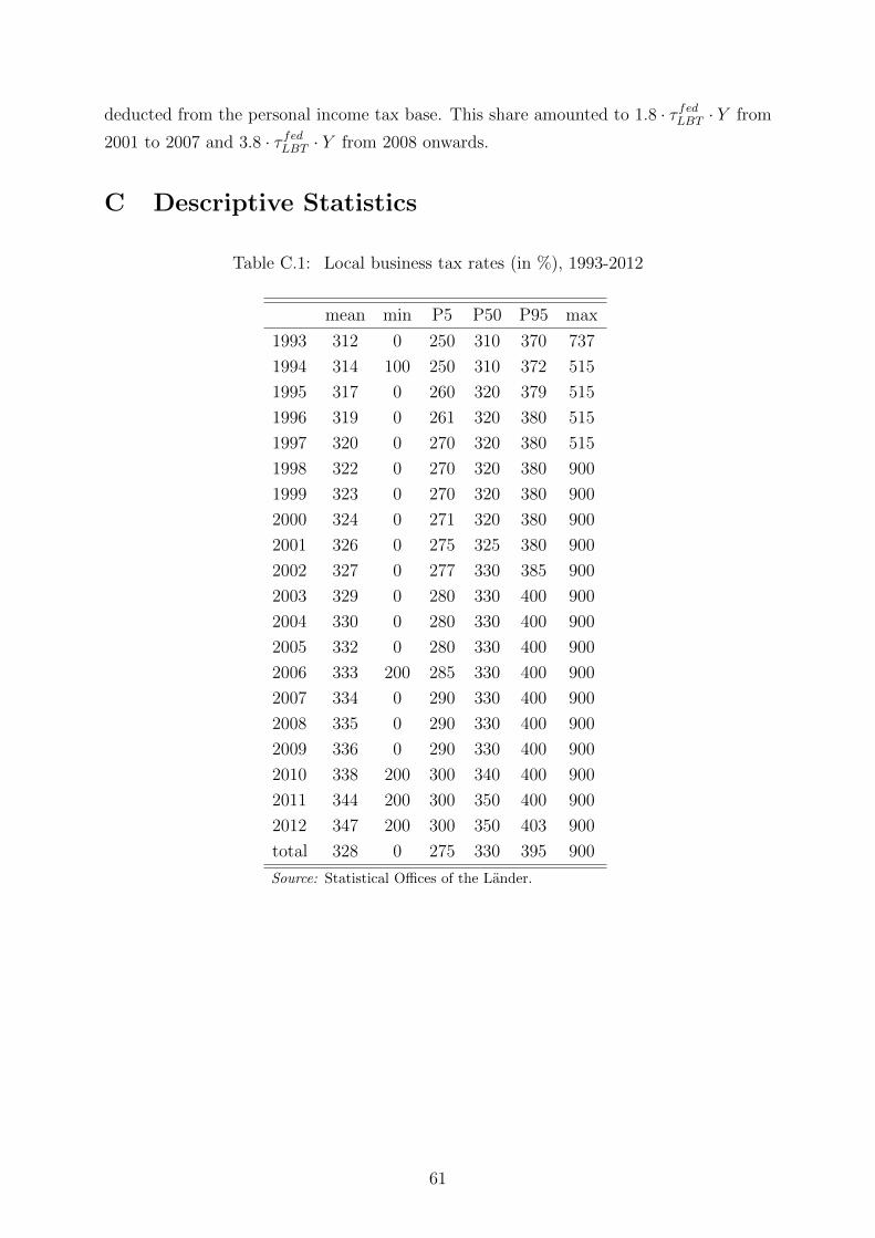
deducted from the personal income tax base. This share amounted to 1.8 · τ fedLBT · Y from

2001 to 2007 and 3.8 · τ fedLBT · Y from 2008 onwards.

C Descriptive Statistics

Table C.1: Local business tax rates (in %), 1993-2012

mean min P5 P50 P95 max

1993 312 0 250 310 370 737

1994 314 100 250 310 372 515

1995 317 0 260 320 379 515

1996 319 0 261 320 380 515

1997 320 0 270 320 380 515

1998 322 0 270 320 380 900

1999 323 0 270 320 380 900

2000 324 0 271 320 380 900

2001 326 0 275 325 380 900

2002 327 0 277 330 385 900

2003 329 0 280 330 400 900

2004 330 0 280 330 400 900

2005 332 0 280 330 400 900

2006 333 200 285 330 400 900

2007 334 0 290 330 400 900

2008 335 0 290 330 400 900

2009 336 0 290 330 400 900

2010 338 200 300 340 400 900

2011 344 200 300 350 400 900

2012 347 200 300 350 403 900

total 328 0 275 330 395 900

Source: Statistical Offices of the Lander.

61

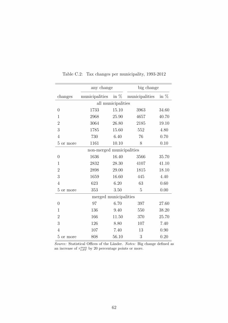
Table C.2: Tax changes per municipality, 1993-2012

any change big change

changes municipalities in % municipalities in %

all municipalities

0 1733 15.10 3963 34.60

1 2968 25.90 4657 40.70

2 3064 26.80 2185 19.10

3 1785 15.60 552 4.80

4 730 6.40 76 0.70

5 or more 1161 10.10 8 0.10

non-merged municipalities

0 1636 16.40 3566 35.70

1 2832 28.30 4107 41.10

2 2898 29.00 1815 18.10

3 1659 16.60 445 4.40

4 623 6.20 63 0.60

5 or more 353 3.50 5 0.00

merged municipalities

0 97 6.70 397 27.60

1 136 9.40 550 38.20

2 166 11.50 370 25.70

3 126 8.80 107 7.40

4 107 7.40 13 0.90

5 or more 808 56.10 3 0.20

Source: Statistical Offices of the Lander. Notes: Big change defined asan increase of τmunLBT by 20 percentage points or more.

62

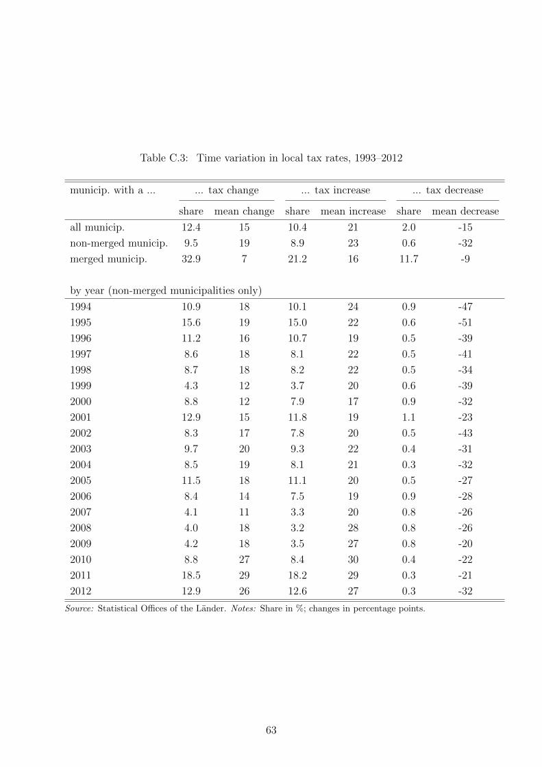
Table C.3: Time variation in local tax rates, 1993–2012

municip. with a ... ... tax change ... tax increase ... tax decrease

share mean change share mean increase share mean decrease

all municip. 12.4 15 10.4 21 2.0 -15

non-merged municip. 9.5 19 8.9 23 0.6 -32

merged municip. 32.9 7 21.2 16 11.7 -9

by year (non-merged municipalities only)

1994 10.9 18 10.1 24 0.9 -47

1995 15.6 19 15.0 22 0.6 -51

1996 11.2 16 10.7 19 0.5 -39

1997 8.6 18 8.1 22 0.5 -41

1998 8.7 18 8.2 22 0.5 -34

1999 4.3 12 3.7 20 0.6 -39

2000 8.8 12 7.9 17 0.9 -32

2001 12.9 15 11.8 19 1.1 -23

2002 8.3 17 7.8 20 0.5 -43

2003 9.7 20 9.3 22 0.4 -31

2004 8.5 19 8.1 21 0.3 -32

2005 11.5 18 11.1 20 0.5 -27

2006 8.4 14 7.5 19 0.9 -28

2007 4.1 11 3.3 20 0.8 -26

2008 4.0 18 3.2 28 0.8 -26

2009 4.2 18 3.5 27 0.8 -20

2010 8.8 27 8.4 30 0.4 -22

2011 18.5 29 18.2 29 0.3 -21

2012 12.9 26 12.6 27 0.3 -32

Source: Statistical Offices of the Lander. Notes: Share in %; changes in percentage points.

63

Table C.4: Descriptive statistics, plant sample, LIAB 1998-2008

mean p50 sd

Wage 2,555 2,539 870

Local tax rate 371 365 52

Share: Tax increases 0.12 0.00 0.33

Share: Tax big decrease 0.03 0.00 0.16

Share: Tax decreases 0.03 0.00 0.17

Municipal expenses (in Thsds.) 312,405 44,560 700,018

Municipal population 98,613 26,456 183,536

District unemployment rate 0.13 0.12 0.06

District GDP (in Mio) 7,667 4,772 10,234

Share: Merged non-merged municipalities 0.72 1.00 0.44

Share: Merged municipalities 0.28 0.00 0.44

Share: West German municipalities 0.62 1.00 0.49

Share: East German municipalities 0.38 0.00 0.49

Number of employees 239 52 1006.06

Value added (in 1000) 129,606 2164 4,950,000

Investments (in 1000) 3212 162 23,425

EBITDA 126,485 777 5,100,000

Share: Liable plants 0.64 1.00 0.48

Share: Non-liable plants 0.36 0.00 0.48

Share: Corporate 0.58 1.00 0.49

Share: Non-corporate 0.42 0.00 0.49

Share: Single plant firms 0.64 1.00 0.48

Share: Part of multi-plant firm 0.36 0.00 0.48

Share: Sector level bargaining 0.54 1.00 0.50

Share: Firm level bargaining 0.09 0.00 0.28

Share: No collective 0.37 0.00 0.48

Share: Manufacturing 0.62 1.00 0.49

Share: Services 0.38 0.00 0.49

Share: High profitability 0.37 0.00 0.48

Share: Medium profitability 0.34 0.00 0.47

Share: Low profitability 0.29 0.00 0.45

Source: LIAB and Statistical Offices of the Lander. Notes: Total number of plant-year observations: 77,357. Number of plants: 21,474. All money variables in 2008euros.

64

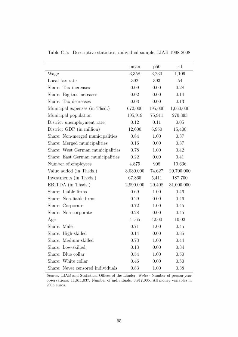
Table C.5: Descriptive statistics, individual sample, LIAB 1998-2008

mean p50 sd

Wage 3,358 3,230 1,109

Local tax rate 392 393 54

Share: Tax increases 0.09 0.00 0.28

Share: Big tax increases 0.02 0.00 0.14

Share: Tax decreases 0.03 0.00 0.13

Municipal expenses (in Thsd.) 672,000 195,000 1,060,000

Municipal population 195,919 75,911 270,393

District unemployment rate 0.12 0.11 0.05

District GDP (in million) 12,600 6,950 15,400

Share: Non-merged municipalities 0.84 1.00 0.37

Share: Merged municipalities 0.16 0.00 0.37

Share: West German municipalities 0.78 1.00 0.42

Share: East German municipalities 0.22 0.00 0.41

Number of employees 4,875 908 10,636

Value added (in Thsds.) 3,030,000 74,627 29,700,000

Investments (in Thsds.) 67,865 5,411 187,700

EBITDA (in Thsds.) 2,990,000 29,408 31,000,000

Share: Liable firms 0.69 1.00 0.46

Share: Non-liable firms 0.29 0.00 0.46

Share: Corporate 0.72 1.00 0.45

Share: Non-corporate 0.28 0.00 0.45

Age 41.65 42.00 10.02

Share: Male 0.71 1.00 0.45

Share: High-skilled 0.14 0.00 0.35

Share: Medium skilled 0.73 1.00 0.44

Share: Low-skilled 0.13 0.00 0.34

Share: Blue collar 0.54 1.00 0.50

Share: White collar 0.46 0.00 0.50

Share: Never censored individuals 0.83 1.00 0.38

Source: LIAB and Statistical Offices of the Lander. Notes: Number of person-yearobservations: 11,611,037. Number of individuals: 3,917,005. All money variables in2008 euros.

65

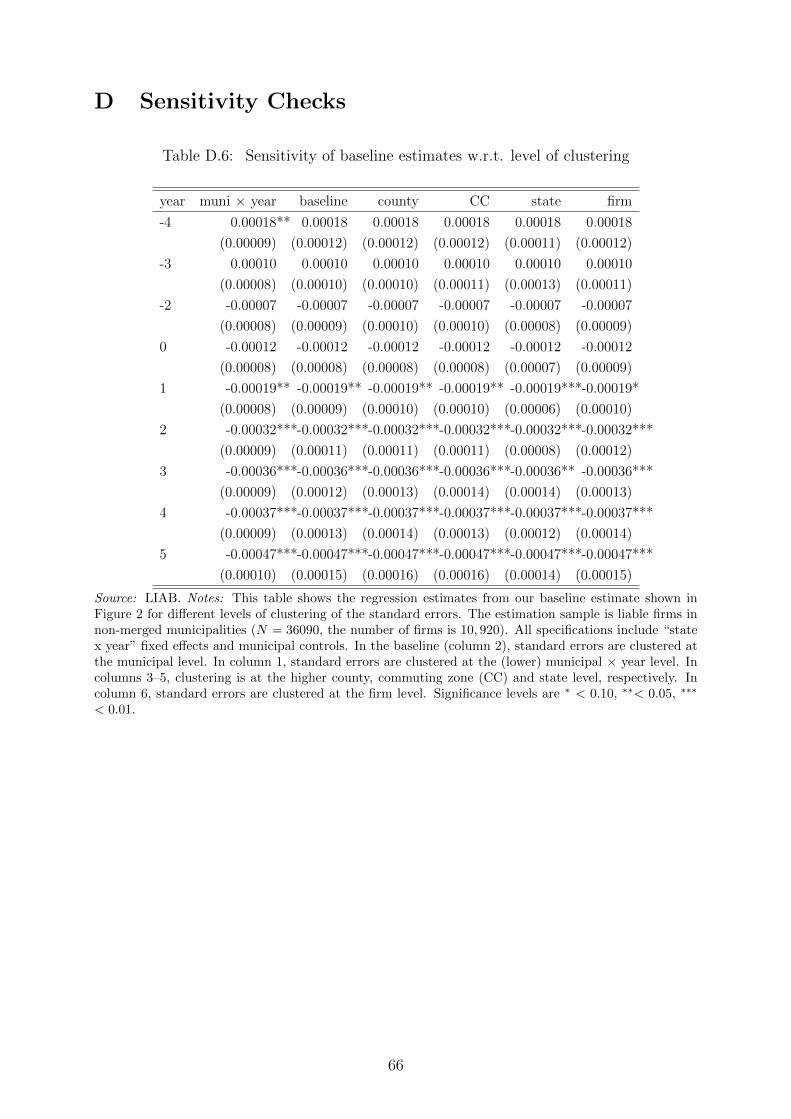
D Sensitivity Checks

Table D.6: Sensitivity of baseline estimates w.r.t. level of clustering

year muni × year baseline county CC state firm

-4 0.00018** 0.00018 0.00018 0.00018 0.00018 0.00018

(0.00009) (0.00012) (0.00012) (0.00012) (0.00011) (0.00012)

-3 0.00010 0.00010 0.00010 0.00010 0.00010 0.00010

(0.00008) (0.00010) (0.00010) (0.00011) (0.00013) (0.00011)

-2 -0.00007 -0.00007 -0.00007 -0.00007 -0.00007 -0.00007

(0.00008) (0.00009) (0.00010) (0.00010) (0.00008) (0.00009)

0 -0.00012 -0.00012 -0.00012 -0.00012 -0.00012 -0.00012

(0.00008) (0.00008) (0.00008) (0.00008) (0.00007) (0.00009)

1 -0.00019** -0.00019** -0.00019** -0.00019** -0.00019***-0.00019*

(0.00008) (0.00009) (0.00010) (0.00010) (0.00006) (0.00010)

2 -0.00032***-0.00032***-0.00032***-0.00032***-0.00032***-0.00032***

(0.00009) (0.00011) (0.00011) (0.00011) (0.00008) (0.00012)

3 -0.00036***-0.00036***-0.00036***-0.00036***-0.00036** -0.00036***

(0.00009) (0.00012) (0.00013) (0.00014) (0.00014) (0.00013)

4 -0.00037***-0.00037***-0.00037***-0.00037***-0.00037***-0.00037***

(0.00009) (0.00013) (0.00014) (0.00013) (0.00012) (0.00014)

5 -0.00047***-0.00047***-0.00047***-0.00047***-0.00047***-0.00047***

(0.00010) (0.00015) (0.00016) (0.00016) (0.00014) (0.00015)

Source: LIAB. Notes: This table shows the regression estimates from our baseline estimate shown inFigure 2 for different levels of clustering of the standard errors. The estimation sample is liable firms innon-merged municipalities (N = 36090, the number of firms is 10, 920). All specifications include “statex year” fixed effects and municipal controls. In the baseline (column 2), standard errors are clustered atthe municipal level. In column 1, standard errors are clustered at the (lower) municipal × year level. Incolumns 3–5, clustering is at the higher county, commuting zone (CC) and state level, respectively. Incolumn 6, standard errors are clustered at the firm level. Significance levels are ∗ < 0.10, ∗∗< 0.05, ∗∗∗

< 0.01.

66

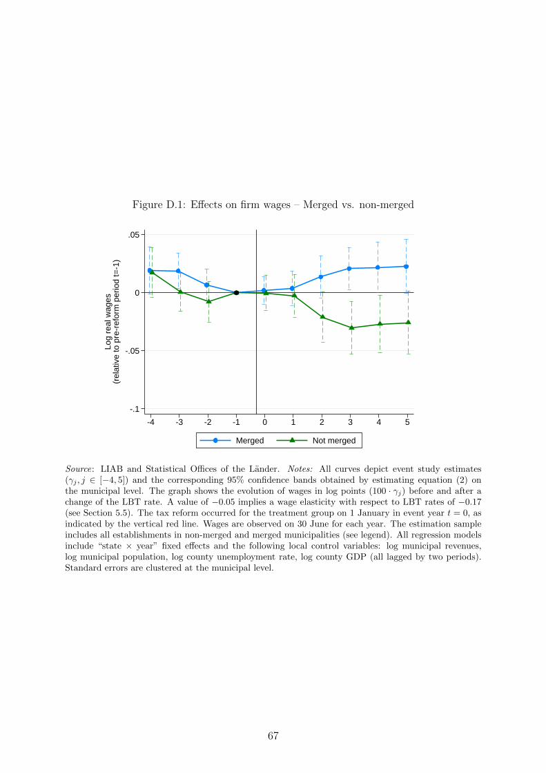
Figure D.1: Effects on firm wages – Merged vs. non-merged

-.1

-.05

0

.05

Log

real

wag

es(r

elat

ive

to p

re-r

efor

m p

erio

d t=

-1)

-4 -3 -2 -1 0 1 2 3 4 5

Merged Not merged

Source: LIAB and Statistical Offices of the Lander. Notes: All curves depict event study estimates(γj , j ∈ [−4, 5]) and the corresponding 95% confidence bands obtained by estimating equation (2) onthe municipal level. The graph shows the evolution of wages in log points (100 · γj) before and after achange of the LBT rate. A value of −0.05 implies a wage elasticity with respect to LBT rates of −0.17(see Section 5.5). The tax reform occurred for the treatment group on 1 January in event year t = 0, asindicated by the vertical red line. Wages are observed on 30 June for each year. The estimation sampleincludes all establishments in non-merged and merged municipalities (see legend). All regression modelsinclude “state × year” fixed effects and the following local control variables: log municipal revenues,log municipal population, log county unemployment rate, log county GDP (all lagged by two periods).Standard errors are clustered at the municipal level.

67

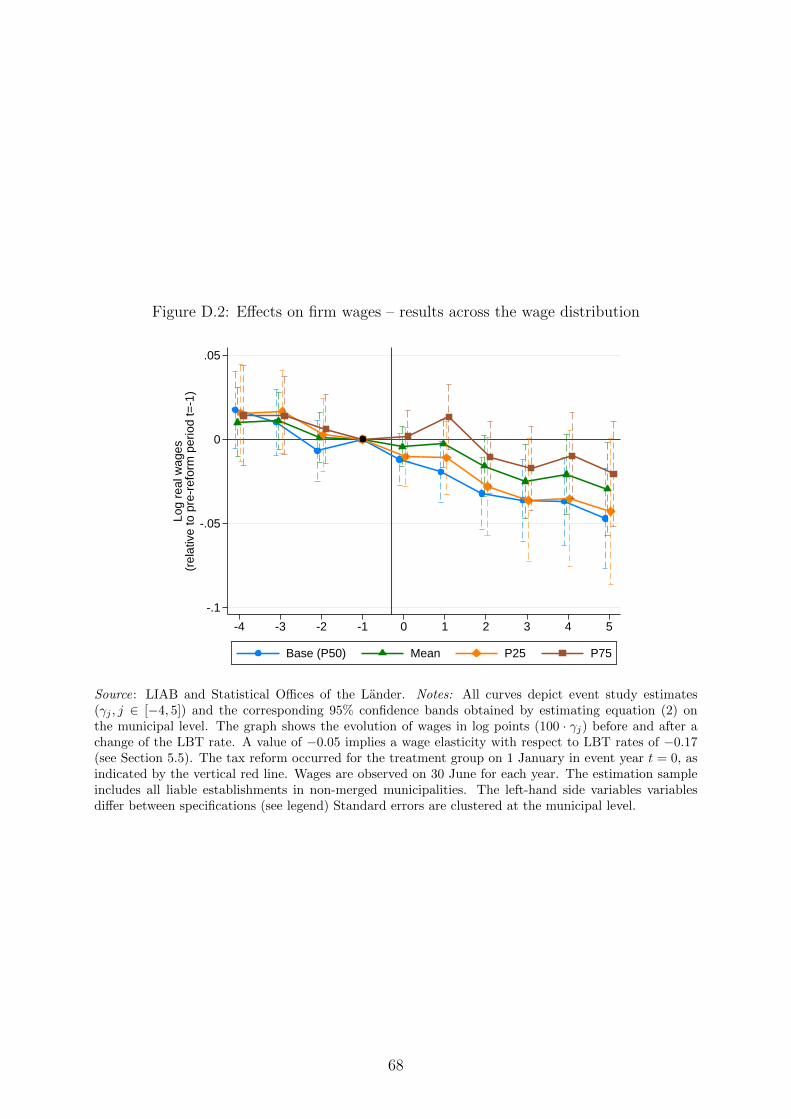
Figure D.2: Effects on firm wages – results across the wage distribution

-.1

-.05

0

.05

Log

real

wag

es(r

elat

ive

to p

re-r

efor

m p

erio

d t=

-1)

-4 -3 -2 -1 0 1 2 3 4 5

Base (P50) Mean P25 P75

Source: LIAB and Statistical Offices of the Lander. Notes: All curves depict event study estimates(γj , j ∈ [−4, 5]) and the corresponding 95% confidence bands obtained by estimating equation (2) onthe municipal level. The graph shows the evolution of wages in log points (100 · γj) before and after achange of the LBT rate. A value of −0.05 implies a wage elasticity with respect to LBT rates of −0.17(see Section 5.5). The tax reform occurred for the treatment group on 1 January in event year t = 0, asindicated by the vertical red line. Wages are observed on 30 June for each year. The estimation sampleincludes all liable establishments in non-merged municipalities. The left-hand side variables variablesdiffer between specifications (see legend) Standard errors are clustered at the municipal level.

68

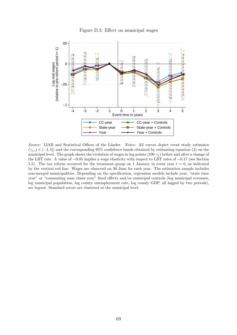
Figure D.3: Effect on municipal wages

-.1

-.05

0

.05

Log

real

wag

es(r

elat

ive

to p

re-r

efor

m p

erio

d t=

-1)

-4 -3 -2 -1 0 1 2 3 4 5Event time in years

CC-year CC-year + ControlsState-year State-year + ControlsYear Year + Controls

Source: LIAB and Statistical Offices of the Lander. Notes: All curves depict event study estimates(γj , j ∈ [−4, 5]) and the corresponding 95% confidence bands obtained by estimating equation (2) on themunicipal level. The graph shows the evolution of wages in log points (100·γj) before and after a change ofthe LBT rate. A value of −0.05 implies a wage elasticity with respect to LBT rates of −0.17 (see Section5.5). The tax reform occurred for the treatment group on 1 January in event year t = 0, as indicatedby the vertical red line. Wages are observed on 30 June for each year. The estimation sample includesnon-merged municipalities. Depending on the specification, regression models include year, “state timeyear” or “commuting zone times year” fixed effects and/or municipal controls (log municipal revenues,log municipal population, log county unemployment rate, log county GDP, all lagged by two periods),see legend. Standard errors are clustered at the municipal level.

69

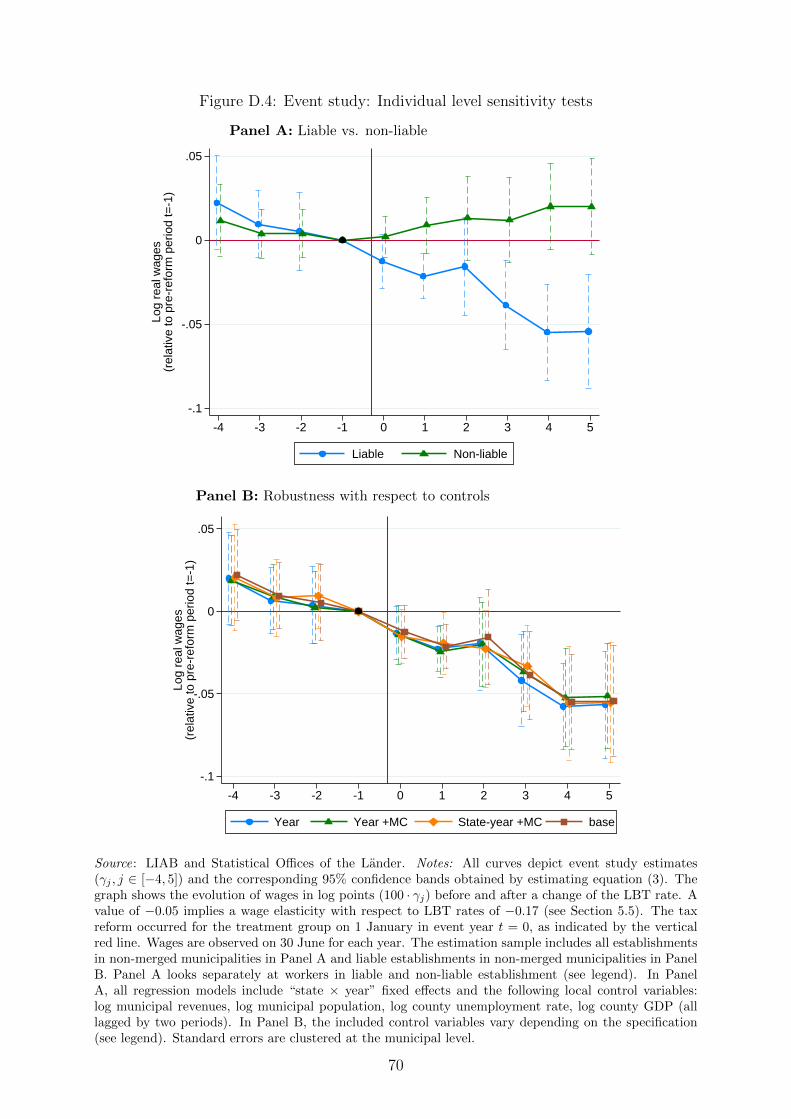
Figure D.4: Event study: Individual level sensitivity tests

Panel A: Liable vs. non-liable

-.1

-.05

0

.05Lo

g re

al w

ages

(rel

ativ

e to

pre

-ref

orm

per

iod

t=-1

)

-4 -3 -2 -1 0 1 2 3 4 5

Liable Non-liable

Panel B: Robustness with respect to controls

-.1

-.05

0

.05

Log

real

wag

es(r

elat

ive

to p

re-r

efor

m p

erio

d t=

-1)

-4 -3 -2 -1 0 1 2 3 4 5

Year Year +MC State-year +MC base

Source: LIAB and Statistical Offices of the Lander. Notes: All curves depict event study estimates(γj , j ∈ [−4, 5]) and the corresponding 95% confidence bands obtained by estimating equation (3). Thegraph shows the evolution of wages in log points (100 · γj) before and after a change of the LBT rate. Avalue of −0.05 implies a wage elasticity with respect to LBT rates of −0.17 (see Section 5.5). The taxreform occurred for the treatment group on 1 January in event year t = 0, as indicated by the verticalred line. Wages are observed on 30 June for each year. The estimation sample includes all establishmentsin non-merged municipalities in Panel A and liable establishments in non-merged municipalities in PanelB. Panel A looks separately at workers in liable and non-liable establishment (see legend). In PanelA, all regression models include “state × year” fixed effects and the following local control variables:log municipal revenues, log municipal population, log county unemployment rate, log county GDP (alllagged by two periods). In Panel B, the included control variables vary depending on the specification(see legend). Standard errors are clustered at the municipal level.

70

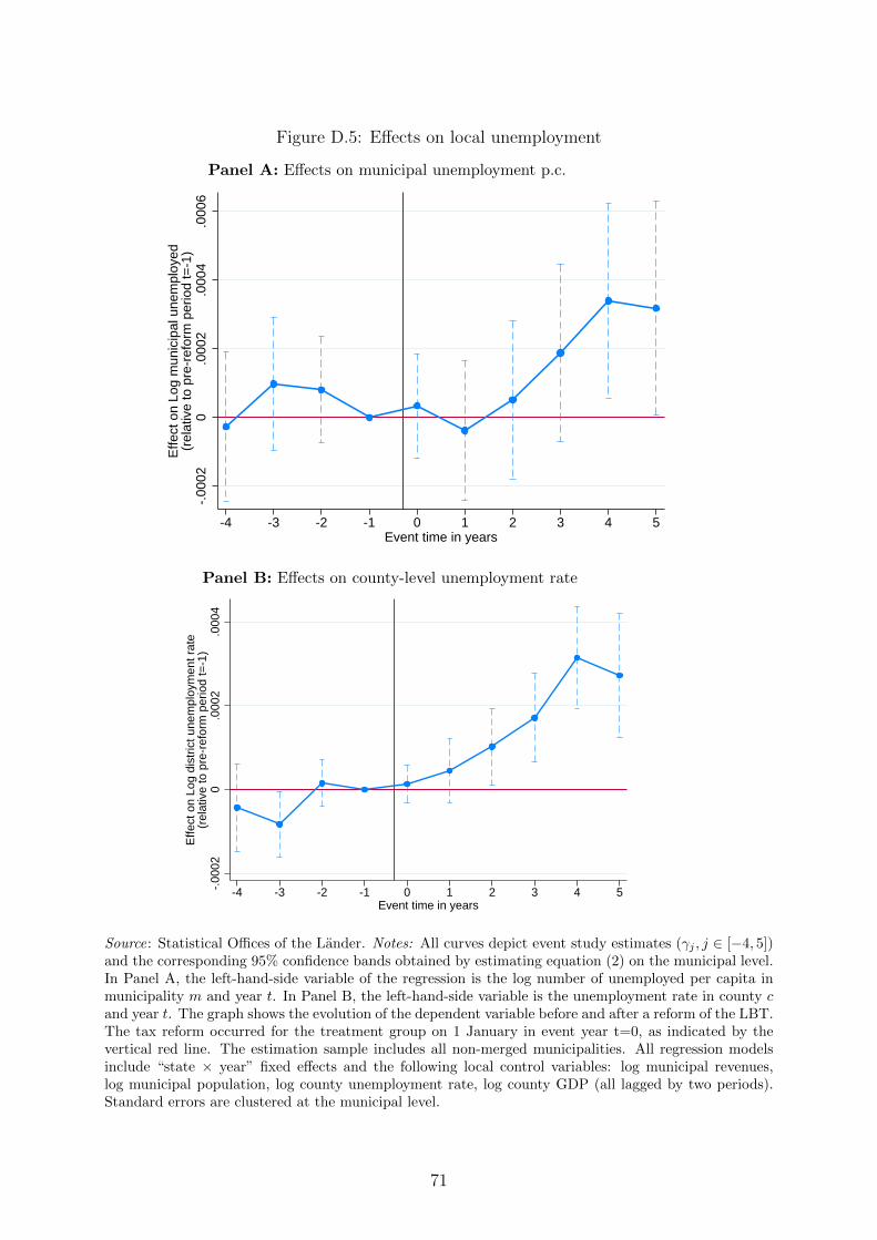
Figure D.5: Effects on local unemployment

Panel A: Effects on municipal unemployment p.c.

-.00

020

.000

2.0

004

.000

6

Effe

ct o

n Lo

g m

unic

ipal

une

mpl

oyed

(rel

ativ

e to

pre

-ref

orm

per

iod

t=-1

)

-4 -3 -2 -1 0 1 2 3 4 5Event time in years

Panel B: Effects on county-level unemployment rate

-.00

020

.000

2.0

004

Effe

ct o

n Lo

g di

stric

t une

mpl

oym

ent r

ate

(rel

ativ

e to

pre

-ref

orm

per

iod

t=-1

)

-4 -3 -2 -1 0 1 2 3 4 5Event time in years

Source: Statistical Offices of the Lander. Notes: All curves depict event study estimates (γj , j ∈ [−4, 5])and the corresponding 95% confidence bands obtained by estimating equation (2) on the municipal level.In Panel A, the left-hand-side variable of the regression is the log number of unemployed per capita inmunicipality m and year t. In Panel B, the left-hand-side variable is the unemployment rate in county cand year t. The graph shows the evolution of the dependent variable before and after a reform of the LBT.The tax reform occurred for the treatment group on 1 January in event year t=0, as indicated by thevertical red line. The estimation sample includes all non-merged municipalities. All regression modelsinclude “state × year” fixed effects and the following local control variables: log municipal revenues,log municipal population, log county unemployment rate, log county GDP (all lagged by two periods).Standard errors are clustered at the municipal level.

71

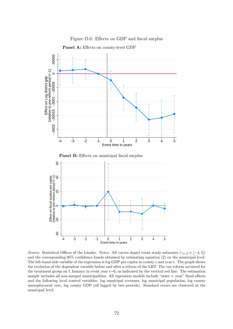
Figure D.6: Effects on GDP and fiscal surplus

Panel A: Effects on county-level GDP-.

0002

-.00

015

-.00

01-.

0000

50

.000

05

Effe

ct o

n Lo

g di

stric

t gdp

(rel

ativ

e to

pre

-ref

orm

per

iod

t=-1

)

-4 -3 -2 -1 0 1 2 3 4 5Event time in years

Panel B: Effects on municipal fiscal surplus

-40

-20

020

4060

Effe

ct o

n fis

cal s

urpl

us p

er c

apita

(rel

ativ

e to

pre

-ref

orm

per

iod

t=-1

)

-4 -3 -2 -1 0 1 2 3 4 5Event time in years

Source: Statistical Offices of the Lander. Notes: All curves depict event study estimates (γj , j ∈ [−4, 5])and the corresponding 95% confidence bands obtained by estimating equation (2) on the municipal level.The left-hand-side variable of the regression is log GDP per capita in county c and year t. The graph showsthe evolution of the dependent variable before and after a reform of the LBT. The tax reform occurred forthe treatment group on 1 January in event year t=0, as indicated by the vertical red line. The estimationsample includes all non-merged municipalities. All regression models include “state × year” fixed effectsand the following local control variables: log municipal revenues, log municipal population, log countyunemployment rate, log county GDP (all lagged by two periods). Standard errors are clustered at themunicipal level.

72

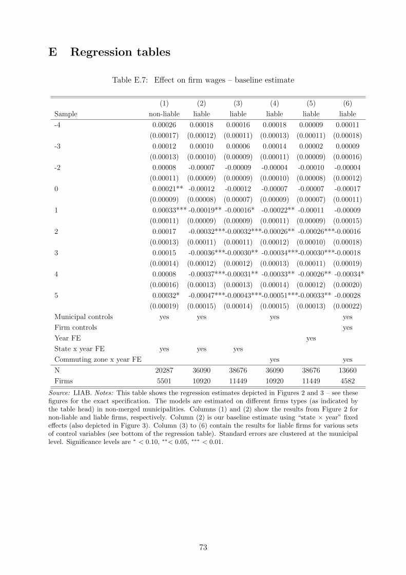
E Regression tables

Table E.7: Effect on firm wages – baseline estimate

(1) (2) (3) (4) (5) (6)

Sample non-liable liable liable liable liable liable

-4 0.00026 0.00018 0.00016 0.00018 0.00009 0.00011

(0.00017) (0.00012) (0.00011) (0.00013) (0.00011) (0.00018)

-3 0.00012 0.00010 0.00006 0.00014 0.00002 0.00009

(0.00013) (0.00010) (0.00009) (0.00011) (0.00009) (0.00016)

-2 0.00008 -0.00007 -0.00009 -0.00004 -0.00010 -0.00004

(0.00011) (0.00009) (0.00009) (0.00010) (0.00008) (0.00012)

0 0.00021** -0.00012 -0.00012 -0.00007 -0.00007 -0.00017

(0.00009) (0.00008) (0.00007) (0.00009) (0.00007) (0.00011)

1 0.00033*** -0.00019** -0.00016* -0.00022** -0.00011 -0.00009

(0.00011) (0.00009) (0.00009) (0.00011) (0.00009) (0.00015)

2 0.00017 -0.00032***-0.00032***-0.00026** -0.00026***-0.00016

(0.00013) (0.00011) (0.00011) (0.00012) (0.00010) (0.00018)

3 0.00015 -0.00036***-0.00030** -0.00034***-0.00030***-0.00018

(0.00014) (0.00012) (0.00012) (0.00013) (0.00011) (0.00019)

4 0.00008 -0.00037***-0.00031** -0.00033** -0.00026** -0.00034*

(0.00016) (0.00013) (0.00013) (0.00014) (0.00012) (0.00020)

5 0.00032* -0.00047***-0.00043***-0.00051***-0.00033** -0.00028

(0.00019) (0.00015) (0.00014) (0.00015) (0.00013) (0.00022)

Municipal controls yes yes yes yes

Firm controls yes

Year FE yes

State x year FE yes yes yes

Commuting zone x year FE yes yes

N 20287 36090 38676 36090 38676 13660

Firms 5501 10920 11449 10920 11449 4582

Source: LIAB. Notes: This table shows the regression estimates depicted in Figures 2 and 3 – see thesefigures for the exact specification. The models are estimated on different firms types (as indicated bythe table head) in non-merged municipalities. Columns (1) and (2) show the results from Figure 2 fornon-liable and liable firms, respectively. Column (2) is our baseline estimate using “state × year” fixedeffects (also depicted in Figure 3). Column (3) to (6) contain the results for liable firms for various setsof control variables (see bottom of the regression table). Standard errors are clustered at the municipallevel. Significance levels are ∗ < 0.10, ∗∗< 0.05, ∗∗∗ < 0.01.

73

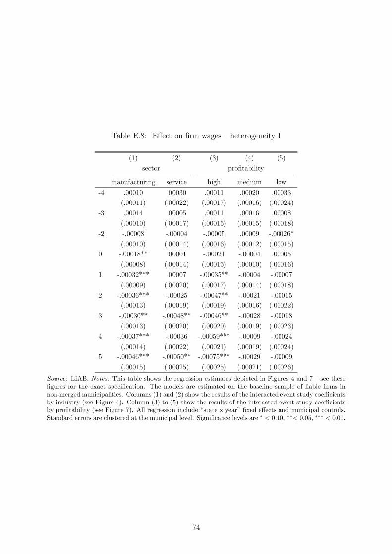
Table E.8: Effect on firm wages – heterogeneity I

(1) (2) (3) (4) (5)

sector profitability

manufacturing service high medium low

-4 .00010 .00030 .00011 .00020 .00033

(.00011) (.00022) (.00017) (.00016) (.00024)

-3 .00014 .00005 .00011 .00016 .00008

(.00010) (.00017) (.00015) (.00015) (.00018)

-2 -.00008 -.00004 -.00005 .00009 -.00026*

(.00010) (.00014) (.00016) (.00012) (.00015)

0 -.00018** .00001 -.00021 -.00004 .00005

(.00008) (.00014) (.00015) (.00010) (.00016)

1 -.00032*** .00007 -.00035** -.00004 -.00007

(.00009) (.00020) (.00017) (.00014) (.00018)

2 -.00036*** -.00025 -.00047** -.00021 -.00015

(.00013) (.00019) (.00019) (.00016) (.00022)

3 -.00030** -.00048** -.00046** -.00028 -.00018

(.00013) (.00020) (.00020) (.00019) (.00023)

4 -.00037*** -.00036 -.00059*** -.00009 -.00024

(.00014) (.00022) (.00021) (.00019) (.00024)

5 -.00046*** -.00050** -.00075*** -.00029 -.00009

(.00015) (.00025) (.00025) (.00021) (.00026)

Source: LIAB. Notes: This table shows the regression estimates depicted in Figures 4 and 7 – see thesefigures for the exact specification. The models are estimated on the baseline sample of liable firms innon-merged municipalities. Columns (1) and (2) show the results of the interacted event study coefficientsby industry (see Figure 4). Column (3) to (5) show the results of the interacted event study coefficientsby profitability (see Figure 7). All regression include “state x year” fixed effects and municipal controls.Standard errors are clustered at the municipal level. Significance levels are ∗ < 0.10, ∗∗< 0.05, ∗∗∗ < 0.01.

74

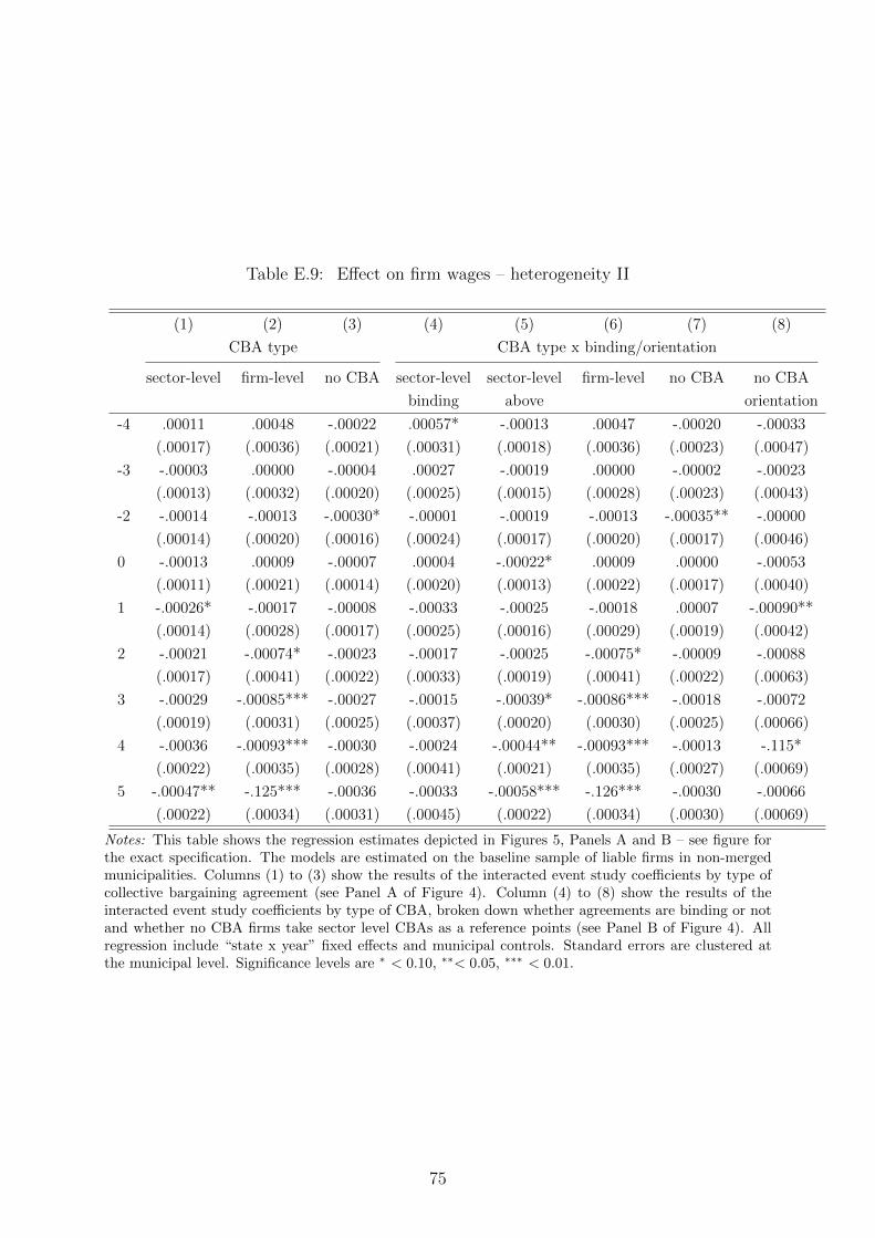
Table E.9: Effect on firm wages – heterogeneity II

(1) (2) (3) (4) (5) (6) (7) (8)

CBA type CBA type x binding/orientation

sector-level firm-level no CBA sector-level sector-level firm-level no CBA no CBA

binding above orientation

-4 .00011 .00048 -.00022 .00057* -.00013 .00047 -.00020 -.00033

(.00017) (.00036) (.00021) (.00031) (.00018) (.00036) (.00023) (.00047)

-3 -.00003 .00000 -.00004 .00027 -.00019 .00000 -.00002 -.00023

(.00013) (.00032) (.00020) (.00025) (.00015) (.00028) (.00023) (.00043)

-2 -.00014 -.00013 -.00030* -.00001 -.00019 -.00013 -.00035** -.00000

(.00014) (.00020) (.00016) (.00024) (.00017) (.00020) (.00017) (.00046)

0 -.00013 .00009 -.00007 .00004 -.00022* .00009 .00000 -.00053

(.00011) (.00021) (.00014) (.00020) (.00013) (.00022) (.00017) (.00040)

1 -.00026* -.00017 -.00008 -.00033 -.00025 -.00018 .00007 -.00090**

(.00014) (.00028) (.00017) (.00025) (.00016) (.00029) (.00019) (.00042)

2 -.00021 -.00074* -.00023 -.00017 -.00025 -.00075* -.00009 -.00088

(.00017) (.00041) (.00022) (.00033) (.00019) (.00041) (.00022) (.00063)

3 -.00029 -.00085*** -.00027 -.00015 -.00039* -.00086*** -.00018 -.00072

(.00019) (.00031) (.00025) (.00037) (.00020) (.00030) (.00025) (.00066)

4 -.00036 -.00093*** -.00030 -.00024 -.00044** -.00093*** -.00013 -.115*

(.00022) (.00035) (.00028) (.00041) (.00021) (.00035) (.00027) (.00069)

5 -.00047** -.125*** -.00036 -.00033 -.00058*** -.126*** -.00030 -.00066

(.00022) (.00034) (.00031) (.00045) (.00022) (.00034) (.00030) (.00069)

Notes: This table shows the regression estimates depicted in Figures 5, Panels A and B – see figure forthe exact specification. The models are estimated on the baseline sample of liable firms in non-mergedmunicipalities. Columns (1) to (3) show the results of the interacted event study coefficients by type ofcollective bargaining agreement (see Panel A of Figure 4). Column (4) to (8) show the results of theinteracted event study coefficients by type of CBA, broken down whether agreements are binding or notand whether no CBA firms take sector level CBAs as a reference points (see Panel B of Figure 4). Allregression include “state x year” fixed effects and municipal controls. Standard errors are clustered atthe municipal level. Significance levels are ∗ < 0.10, ∗∗< 0.05, ∗∗∗ < 0.01.

75

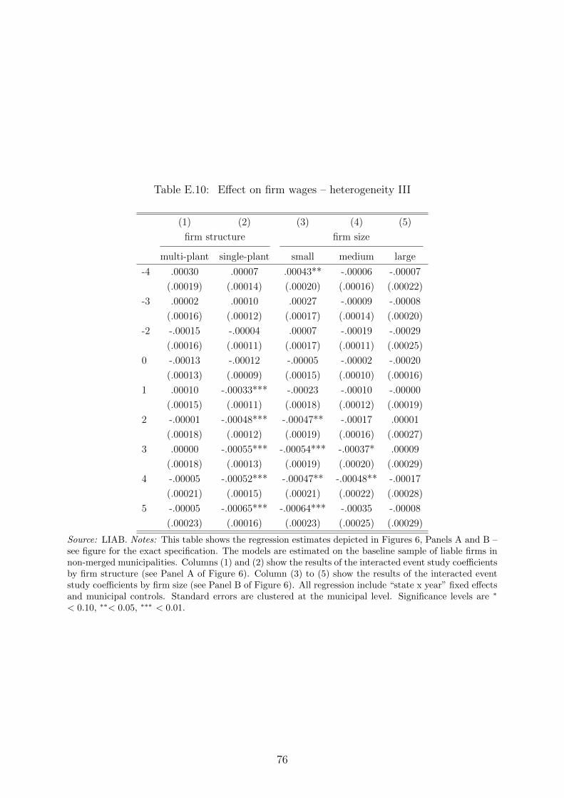
Table E.10: Effect on firm wages – heterogeneity III

(1) (2) (3) (4) (5)

firm structure firm size

multi-plant single-plant small medium large

-4 .00030 .00007 .00043** -.00006 -.00007

(.00019) (.00014) (.00020) (.00016) (.00022)

-3 .00002 .00010 .00027 -.00009 -.00008

(.00016) (.00012) (.00017) (.00014) (.00020)

-2 -.00015 -.00004 .00007 -.00019 -.00029

(.00016) (.00011) (.00017) (.00011) (.00025)

0 -.00013 -.00012 -.00005 -.00002 -.00020

(.00013) (.00009) (.00015) (.00010) (.00016)

1 .00010 -.00033*** -.00023 -.00010 -.00000

(.00015) (.00011) (.00018) (.00012) (.00019)

2 -.00001 -.00048*** -.00047** -.00017 .00001

(.00018) (.00012) (.00019) (.00016) (.00027)

3 .00000 -.00055*** -.00054*** -.00037* .00009

(.00018) (.00013) (.00019) (.00020) (.00029)

4 -.00005 -.00052*** -.00047** -.00048** -.00017

(.00021) (.00015) (.00021) (.00022) (.00028)

5 -.00005 -.00065*** -.00064*** -.00035 -.00008

(.00023) (.00016) (.00023) (.00025) (.00029)

Source: LIAB. Notes: This table shows the regression estimates depicted in Figures 6, Panels A and B –see figure for the exact specification. The models are estimated on the baseline sample of liable firms innon-merged municipalities. Columns (1) and (2) show the results of the interacted event study coefficientsby firm structure (see Panel A of Figure 6). Column (3) to (5) show the results of the interacted eventstudy coefficients by firm size (see Panel B of Figure 6). All regression include “state x year” fixed effectsand municipal controls. Standard errors are clustered at the municipal level. Significance levels are ∗

< 0.10, ∗∗< 0.05, ∗∗∗ < 0.01.

76

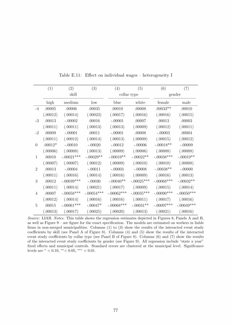
Table E.11: Effect on individual wages – heterogeneity I

(1) (2) (3) (4) (5) (6) (7)

skill collar type gender

high medium low blue white female male

-4 .00005 .00006 .00035 .00010 .00008 .00033** .00010

(.00012) (.00014) (.00023) (.00017) (.00016) (.00016) (.00015)

-3 .00013 -.00002 .00016 -.00001 .00007 .00013 .00003

(.00011) (.00011) (.00013) (.00013) (.00009) (.00012) (.00011)

-2 .00009 -.00001 .00011 -.00001 .00008 -.00003 .00004

(.00011) (.00012) (.00014) (.00013) (.00009) (.00015) (.00012)

0 .00012* -.00010 -.00020 -.00012 -.00006 -.00018** -.00009

(.00006) (.00008) (.00013) (.00009) (.00006) (.00008) (.00008)

1 .00010 -.00021*** -.00029** -.00019** -.00022** -.00038*** -.00019**

(.00007) (.00007) (.00012) (.00009) (.00010) (.00010) (.00008)

2 .00013 -.00004 -.00011 -.00003 -.00008 -.00038** -.00000

(.00011) (.00016) (.00014) (.00016) (.00009) (.00016) (.00013)

3 .00012 -.00039*** -.00030 -.00040** -.00025*** -.00068*** -.00032**

(.00011) (.00014) (.00021) (.00017) (.00009) (.00015) (.00014)

4 .00007 -.00058*** -.00054*** -.00062*** -.00035*** -.00090*** -.00050***

(.00012) (.00014) (.00016) (.00016) (.00011) (.00017) (.00016)

5 .00015 -.00061*** -.00047* -.00068*** -.00031** -.00097*** -.00049***

(.00013) (.00017) (.00025) (.00020) (.00013) (.00021) (.00016)

Source: LIAB. Notes: This table shows the regression estimates depicted in Figures 8, Panels A and B,as well as Figure 9 – see figure for the exact specification. The models are estimated on workers in liablefirms in non-merged municipalities. Columns (1) to (3) show the results of the interacted event studycoefficients by skill (see Panel A of Figure 8). Columns (4) and (5) show the results of the interactedevent study coefficients by collar type (see Panel B of Figure 8). Columns (6) and (7) show the resultsof the interacted event study coefficients by gender (see Figure 9). All regression include “state x year”fixed effects and municipal controls. Standard errors are clustered at the municipal level. Significancelevels are ∗ < 0.10, ∗∗< 0.05, ∗∗∗ < 0.01.

77