Embed Size (px)
Citation preview
DEMOGRAPHIC RESEARCH VOLUME 32, ARTICLE 26, PAGES 797−828 PUBLISHED 25 MARCH 2015 http://www.demographic-research.org/Volumes/Vol32/26/ DOI: 10.4054/DemRes.2015.32.26 Research Article
Do low survey response rates bias results? Evidence from Japan
Ronald R. Rindfuss
Minja K. Choe
Noriko O. Tsuya
Larry L. Bumpass
Emi Tamaki
©2015 Rindfuss, Choe, Tsuya, Bumpass & Tamaki. This open-access work is published under the terms of the Creative Commons Attribution NonCommercial License 2.0 Germany, which permits use, reproduction & distribution in any medium for non-commercial purposes, provided the original author(s) and source are given credit. See http:// creativecommons.org/licenses/by-nc/2.0/de/

Table of Contents
1 Introduction 798 2 Decline in respondent cooperation 799 3 Factors and mechanisms affecting survey response rates 802 4 Data 804 5 Some terminology and the logic behind our analysis 805 6 Results 808 6.1 Response rates by demographic characteristics 808 6.2 Distributional bias 812 6.3 Relational bias 812 6.4 Life course events and panel retention 813 7 Summary 815 8 Discussion 816 8.1 Our results and common intuition 816 8.2 Paradata 817 8.3 Extra effort/incentives at the end of fieldwork: An improvement or
not? 818
9 Acknowledgements 819 References 820 Appendix 827
Demographic Research: Volume 32, Article 26 Research Article
http://www.demographic-research.org 797
Do low survey response rates bias results? Evidence from Japan
Ronald R. Rindfuss1
Minja K. Choe2
Noriko O. Tsuya3
Larry L. Bumpass4
Emi Tamaki5
Abstract
BACKGROUND In developed countries, response rates have dropped to such low levels that many in the population field question whether the data can provide unbiased results.
OBJECTIVE The paper uses three Japanese surveys conducted in the 2000s to ask whether low survey response rates bias results. A secondary objective is to bring results reported in the survey response literature to the attention of the demographic research community.
METHODS Using a longitudinal survey as well as paradata from a cross-sectional survey, a variety of statistical techniques (chi square, analysis of variance (ANOVA), logistic regression, ordered probit or ordinary least squares regression (OLS), as appropriate) are used to examine response-rate bias.
RESULTS Evidence of response-rate bias is found for the univariate distributions of some demographic characteristics, behaviors, and attitudinal items. But when examining relationships between variables in a multivariate analysis, controlling for a variety of background variables, for most dependent variables we do not find evidence of bias from low response rates.
1 East-West Center and University of North Carolina at Chapel Hill, U.S.A. E-Mail: [email protected]. 2 East-West Center, U.S.A. 3 Keio University, Japan. 4 University of Wisconsin–Madison, U.S.A. 5 Ritsumeikan University, Japan.
Rindfuss et al.: Do low survey response rates bias results? Evidence from Japan
798 http://www.demographic-research.org
CONCLUSIONS Our results are consistent with results reported in the econometric and survey research literatures. Low response rates need not necessarily lead to biased results. Bias is more likely to be present when examining a simple univariate distribution than when examining the relationship between variables in a multivariate model.
COMMENTS The results have two implications. First, demographers should not presume the presence or absence of low response-rate bias; rather they should test for it in the context of a specific substantive analysis. Second, demographers should lobby data gatherers to collect as much paradata as possible so that rigorous tests for low response-rate bias are possible.
1. Introduction
Sample surveys (cross-sectional and longitudinal) have become the dominant data source used by population researchers. Response rates, both the initial response rate and attrition rates in longitudinal studies, have historically been an important rough-and-ready yardstick to judge data quality. Response rates6 have been declining in urbanized, high-income countries to the point where many cross-sectional surveys now have response rates below 50% (Atrostic et al. 2001; Brick and Williams 2013; de Leeuw and de Heer 2002; Groves 2011; Singer 2006).
The survey literature has long recognized that low response rates only indicate potential bias (e.g., Lessler and Kalsbeck 1992), yet the almost automatic response among most in the population field has been to equate low response rates with poor data quality. Low response rates produce bias only to the extent that there are differences between responders and non-responders on the estimate(s) of interest, and then only if such differences cannot be eliminated or controlled for through the use of observable and available characteristics of responders and non-responders. The difficulty in evaluating non-response bias is that measures of the variable(s) of interest and characteristics of non-responders are generally not observed, and hence the population field has tended to rely on the presumption that low response rates necessarily mean low data quality.
In this paper, using surveys designed by demographers and variables that have often been used as dependent variables in demographic research, we examine this
6 Non-response can occur for a variety of reasons, including an outright refusal, agreeing to respond but then not being there at the appointed time, and failure on the part of the field worker to contact the potential respondent. We include all reasons for non-response under the “non-response” umbrella.
Demographic Research: Volume 32, Article 26
http://www.demographic-research.org 799
common presumption of demographers. We also place our results in the context of the survey research literature in which there are numerous indications that low response rates need not mean the results are biased and, if there is bias within the survey, it varies considerably from variable to variable. It has been unfortunate that the research literature on response rates and bias has tended to be published in journals aimed at survey research experts. These are journals that tend not to be read by population researchers and hence the persistent belief that low response rates equate to low-quality, biased data.
We examine data quality issues across a range of behavioral, knowledge, and attitudinal variables for two data collection efforts conducted in Japan in 2009, one a follow-up of a cross-sectional survey conducted in 2000 and one a new cross section. Both 2009 efforts were conducted by the same data gathering organization, using the same procedures and the same questionnaire. Both had modest response rates: 53% of those surveyed in 2000 for the longitudinal follow-up and 54% of those sampled from Japan’s basic residence registration for the new cross section. As is shown below, response rates in this range are now typical in Japan and other industrialized countries. To preview our results, we find evidence that low response rates likely bias simple univariate distributions of some behaviors, knowledge, and attitudinal items, but low response rates seem not to bias estimates of the relationship between various independent variables and these behavioral, knowledge, and attitudinal items.
2. Decline in respondent cooperation
Declines in respondent cooperation in developed countries have been widely reported in the survey research literature (e.g., Groves 2011), including government-conducted surveys (e.g., Atrostic et al. 2001; Bethlehem, Cobben, and Schouten 2011; Brick and Williams 2013; de Leeuw and de Heer 2002), and such declines have been going on for many years (Steeh 1981). These declines are easiest to see in cross-sectional surveys that have been repeated over a long period. Consider the University of Michigan’s Survey of Consumer Attitudes (SCA). In the mid-1950s, response rates were close to 90% (Steeh 1981); by 2003, the response rate was below 50% (Curtin, Presser, and Singer 2005). In Japan, the response rate of Mainichi Shimbun’s National Opinion Survey on Family Planning declined from 92% in 1950 to 61% in 2004 (Robert Retherford and Naohiro Ogawa, personal communication). The decline has been even more drastic in telephone polling. Keeter (2012) reports that the response rate on a typical Pew telephone survey dropped from 36% in 1997 to only 9% in 2012. As Dillman and colleagues (2009) note, responding to surveys has changed from being an obligation to being a matter of respondent choice and convenience.
Rindfuss et al.: Do low survey response rates bias results? Evidence from Japan
800 http://www.demographic-research.org
Within data series, further evidence of declining respondent cooperation is the percentage for whom there is missing data. In the U.S. Current Population Survey, the percentage for whom wages had to be imputed increased from 14% in 1983 to 33% in 2008 (Mouw and Kalleberg 2010).
Across countries there appears to be considerable variation in response rates. For example, consider the response rates for wave 1 of the Generations and Gender Programme (Aat Liefbroer, personal communication): Austria 56%, Czech Republic 42%, Estonia 72%, France 56%, Georgia 68%, Germany 55%, Hungary 54%, Italy 79%, Japan 61%, Netherlands 45%, Rumania 84%, and Russia 42%. De Leeuw and de Heer (2002) systematically examined trends in non-response to government surveys across 17 countries from North America, Oceania, and Eastern and Western Europe. They found declines in response rates for all countries, but the trends and levels of non-response differed by country, and the country differences were more the result of refusals rather than noncontacts. Bethlehem and colleagues (2011) show cross-country variation using the European Social Survey. They also find wide country variation in non-response. Furthermore, there is wide variation in the components of non-response: non-contact, refusal, and unable to participate (i.e., due to illness, hearing loss, or language difficulty); and countries may rank high on one component and low on another. The across-country variation suggests there are country-specific factors influencing response rates in addition to factors common across urbanized, industrialized countries. These country-specific factors are part of the social environment in which surveys are conducted (Groves and Couper 1998).
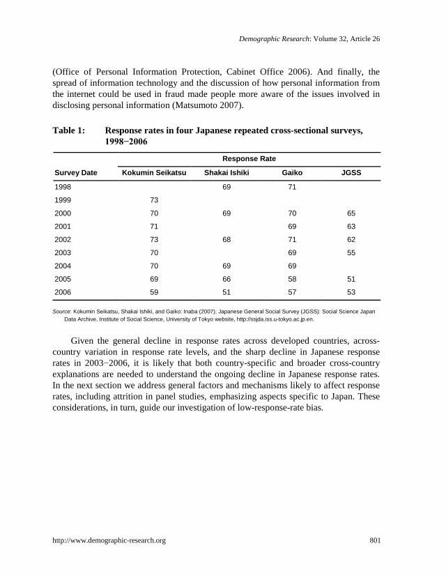
Japanese surveys experienced substantial declines in response rates around the turn of the 21st century. Table 1 shows the response rate trend for four repeated cross-sectional survey programs in Japan from 1998 to 2006. All four are national surveys measuring attitudes on various topics7. As can be seen in Table 1, by 2006 all four had response rates below 60%. Several Japan-specific arguments have been advanced for this dramatic decline. There was a sharp increase in crimes involving fraudulently-obtained personal information used to bilk individuals, which prompted local authorities to warn residents to be wary of dubious calls or visits (Inaba 2007); presumably the wariness of strangers requesting things was extended to field workers for legitimate research projects. There were several widely reported incidents involving the accidental release of personal information, including the 2003 unauthorized release of more than 5 million pieces of personal information for individuals who accessed the Yahoo Japan website. Publicity surrounding the 2003 enactment of the Personal Information Protection Law (Kojin-joho Hogo Ho) heightened awareness of fraudulent use of personal information (Inaba 2007). Enforcement of this law began in 2005
7 More information on the specific survey programs can be found in Inaba (2007) or Synodinos and Yamada (2000).
Demographic Research: Volume 32, Article 26
http://www.demographic-research.org 801
(Office of Personal Information Protection, Cabinet Office 2006). And finally, the spread of information technology and the discussion of how personal information from the internet could be used in fraud made people more aware of the issues involved in disclosing personal information (Matsumoto 2007). Table 1: Response rates in four Japanese repeated cross-sectional surveys,
1998−2006
Response Rate
Survey Date Kokumin Seikatsu Shakai Ishiki Gaiko JGSS
1998
69 71
1999 73
2000 70 69 70 65
2001 71
69 63
2002 73 68 71 62
2003 70
69 55
2004 70 69 69
2005 69 66 58 51
2006 59 51 57 53 Source: Kokumin Seikatsu, Shakai Ishiki, and Gaiko: Inaba (2007); Japanese General Social Survey (JGSS): Social Science Japan
Data Archive, Institute of Social Science, University of Tokyo website, http://ssjda.iss.u-tokyo.ac.jp.en.
Given the general decline in response rates across developed countries, across-
country variation in response rate levels, and the sharp decline in Japanese response rates in 2003−2006, it is likely that both country-specific and broader cross-country explanations are needed to understand the ongoing decline in Japanese response rates. In the next section we address general factors and mechanisms likely to affect response rates, including attrition in panel studies, emphasizing aspects specific to Japan. These considerations, in turn, guide our investigation of low-response-rate bias.
Rindfuss et al.: Do low survey response rates bias results? Evidence from Japan
802 http://www.demographic-research.org
3. Factors and mechanisms affecting survey response rates
Obtaining data from a respondent8 is a social interaction involving potential respondents, data gatherers, and an assortment of intervening barriers and incentives, including the social environment and the survey design (e.g., Dillman, Smyth, and Christian 2009; Groves and Couper 1998). Let us consider potential respondents first. They have interests, psychological predispositions, and obligations, which can make them more or less likely to cooperate with field staff, or even able to be located by field staff. Psychological predispositions are one example (Groves et al. 2009, Figure 2.3). Some people are cooperative, trusting, and/or highly value academic research, while others can be non-cooperative, suspicious, and stingy with their time. And some people might have different thresholds on various dimensions that need to be reached before they are willing to participate, as leverage-saliency theory suggests (Groves, Singer, and Corning 2000). For example, a news story about a confidentiality breach might push them not to respond when otherwise they might have; or their interest in the topic of the survey might make them more likely to respond. Evidence from the U.S. suggests that those not interested in the substantive topic of the research project are more likely to refuse participation (Couper 1997).
Demographic and life-style characteristics of respondents can also influence their willingness to participate. One example involves the time during the week when the potential respondent is contactable. Aspects of their work (including long work hours), hobbies, volunteer activities, commuting, and other activities could make them difficult to reach (e.g., Vercruyssen, van de Putte, and Stoop 2011). Experienced interviewers often schedule their first visit to a potential respondent’s dwelling unit during the daylight hours to obtain clues (e.g., children’s bikes or toys in the yard) about the likely best time to visit the respondent (Groves and Couper 1998). Some might be more likely to change dwelling units because of family-type events (marriage, childbearing, and marital dissolution) or for work-related reasons, thus making them more difficult to be tracked in a longitudinal study (e.g., Sakamoto 2006; Voorpostel and Lipps 2011).
In a panel survey, the respondent’s experience in prior waves can affect their willingness to participate in the current wave (Lepkowski and Couper 2002). To the extent that the previous experience was positive (for example, the respondent enjoyed interacting with the interviewer, and found the questions stimulating) then that person is more likely to participate in the current wave. The obverse is also expected.
Data gatherers also have characteristics that affect the likelihood of potential respondents cooperating, with some having more cachet with potential respondents than
8 There are numerous methods for obtaining information from a respondent, including face-to-face interviews, telephone interviews, web-based interviews, and mail-out-mail-back approaches. For linguistic ease we use the generic term “contact” to represent these different data collection modes.
Demographic Research: Volume 32, Article 26
http://www.demographic-research.org 803
others. A respected government agency or a prestigious university is more likely to elicit a positive response from potential respondents than a commercial marketing company (e.g., Groves et al. 2012). An organization’s procedures, including training given to field workers, could influence response rates. Similarly, field workers vary in their abilities (including training, experience, and basic personality traits), which can affect the likelihood of a potential respondent cooperating (Dijkstra and Smit 2002; Durrant et al. 2010; Maynard, Freese, and Schaeffer 2010; West and Olson 2010). Factors include their outward appearance (mannerisms, age, size, facial expressions, race/ethnicity, and clothing), their cleverness in locating places, and their persuasive abilities. For example, there are country-level differences in data collectors’ attitudes and behaviors, with Canada and Sweden being high on using ‘foot-in-the-door’ approaches9 and Belgium and the Netherlands low (Hox and de Leeuw 2002).
There are also a wide variety of intervening considerations, both obstacles and facilitating factors, that affect the likelihood of successful data collection effort (Dillman, Smyth, and Christian 2009). One example is a gatekeeper between the field worker and the potential respondent’s dwelling unit (Durrant and D’Arigo 2011). This could be a person, such as doormen found in many Manhattan apartment buildings, or an automated system that operates a gate to a community or a front door to an apartment building. With the automated system, the field worker needs to push a button corresponding to the potential respondent’s dwelling unit, and then the audio, and sometimes video, components of the system allow potential respondents to make a decision without having to have a face-to-face encounter with the field worker. Such systems are very common in urbanized Japan. Caller ID functions on phones are a similar obstacle. Within a household there might be a person who usually answers the phone or the door, and that person could facilitate or hinder the likelihood of an interview.
The ease with which it is possible to find a street address is also important, and here Japan presents a special case because building numbers do not necessarily run consecutively on a street or block; rather they sometimes reflect the temporal order in which buildings were built. For panel studies, national postal services can play an important role in forwarding survey plans to panel members who change their dwelling units and informing the sender of the panel member’s new address. In Japan mail is forwarded for one year, but the sender is not notified of the new address. In the U.S., an important source of information for tracing panel study members is commercial services such as InfoUSA (www.infousa.com), Experian (www.experian.com), and Credit Plus (www.creditplus.com). For example, Experian claims to have demographic
9 These are approaches whereby the interviewers attempt to engage the potential respondent, typically at the door of the dwelling unit, in a conversation with the aim of learning what might motivate the potential respondent to participate, and then address those issues to convert the person into being a respondent.
Rindfuss et al.: Do low survey response rates bias results? Evidence from Japan
804 http://www.demographic-research.org
information on 235 million people. Such commercial services are not available in Japan.
Finally, aspects of the general social environment in a country or a neighborhood can affect the likelihood of the potential respondent cooperating with data gatherers. As discussed above, in Japan the publicity surrounding the 2003 enactment of the Act on the Protection of Personal Information (Kojin-joho Hogo Ho) is an example. In the United States, a wide variety of strategies has been used to try to persuade initial refusers to participate in the survey, including increasing the incentive paid to the potential respondent or sending a different interviewer to the address. In Japan, currently, once a potential respondent refuses to be interviewed, it is then illegal to go back and try to persuade him or her to change their mind. Other aspects of the social environment would include perceptions of crime in the neighborhood and group norms regarding cooperation with researchers (e.g., Groves et al. 2006).
4. Data
There are three sources of data for this paper: 1) the 2000 National Survey on Family and Economic Conditions (hereafter “2000 panel”), 2) a 2009 longitudinal follow-up of the 2000 panel (hereafter “2009 panel”), and 3) a new cross-sectional survey, the 2009 National Survey on Family and Economic Conditions (hereafter “2009 cross section”). The 2000 panel and the 2009 cross section were stratified two-stage national probability samples, with the first stage being a sample of geographic primary sampling units (PSUs). In the second stage, Japan’s basic residence registration (jumin kihon daicho) system was used. This system covers the entire resident population and contains each individual’s name, age, sex, and current address. By using the data from the basic residence registration system, unlike the typical cross-sectional survey in the United States (e.g., Lessler and Kalsbeek 1992), we know the age, sex, and place of residence of both responders and non-responders. To evaluate bias in survey data it is crucial to have auxiliary data for both non-respondents and respondents (Bethlehem, Cobben, and Schouten 2011). Japan’s basic residence registration provides auxiliary data on age, sex, and geographic location. The 2009 panel attempted to follow all respondents from 200010, and hence for both responders and non-responders in the 2009 panel all information collected in 2000 is available to serve as auxiliary data. Both the 2000 panel and 2009 cross section were limited to men and women aged 20−49. The 2009 panel has data from 2,356 respondents compared to 4,482 respondents in 2000, and the 2009 cross section has 3,112 respondents.
10 Under Japanese law it was not permissible in 2009 to contact non-responders from the 2000 fieldwork.
Demographic Research: Volume 32, Article 26
http://www.demographic-research.org 805
The 2000 panel was the baseline survey for the panel study. Three hundred and fifty locales were randomly selected based on the 1995 population census tract distribution. Then 20 individuals aged 20−49 were randomly selected within each locale, using the population registers based on current residence. Individuals aged 20−39 were selected at twice the rate of those aged 40−49. Among those selected the response rate varied by place of residence, sex, and age. Sample weights were estimated, inversely proportional to the probability of being selected and responding by age, sex, and place of residence. The design of the 2009 cross section was essentially the same, except that the first sampling stage was based on the 2005 population census tract distribution.
For all three data collection efforts, the mode of data collection is different from those typically used in the U.S. or other Western countries. Potential respondents were first sent a postcard informing them about the project, including its scientific purpose11, and indicating that a field worker would soon visit. Field workers then contacted potential respondents, described the project12, and, if the person agreed to participate, a self-administered questionnaire was left for the respondent to complete and was subsequently picked up by the field worker. When the completed questionnaire was collected, the respondent was given a 2,000 yen (approximately US$25) gift certificate as well as a postcard to notify the survey agency of future address changes. Yamada and Synodinos (1994) report that, in Japan, drop-off pick-up self-administered surveys have higher response rates than personal interviews, but the differences are not large. For the panel, between 2000 and 2009 periodic newsletters and postcards were sent to both keep them informed about the study and to request updated address information if they had moved.
5. Some terminology and the logic behind our analysis
We distinguish between biases that are ‘distributional’ compared to ‘relational’. By distributional, we mean the descriptive features of the univariate distribution of some variable (e.g., proportions, means, or standard deviations), whether a social demographic variable like age or marital status or a more substantive variable like fertility intentions or attitudes. Reporting the percentage of respondents who think that “a preschool-age child suffers if the mother works” would be an example of potential
11 The postcard also indicated that Keio University was the Japanese academic unit responsible for the study, and that Shin Joho Center was the survey organization conducting the fieldwork. 12 When the field worker contacted the potential respondent, he/she was also handed a letter on Keio University letterhead which again described the study, indicated a URL for a Keio University website that explained the study in detail, including phone and fax numbers of Keio University and Shin Joho Center in case the respondent wanted to verify the study’s legitimacy.
Rindfuss et al.: Do low survey response rates bias results? Evidence from Japan
806 http://www.demographic-research.org
distributional non-response bias if the responders differ from the non-responders on this attitudinal item. Relational bias involves the relationship between a set of independent variables and a dependent variable. To continue with “the preschool child suffers” example, we would say that relational bias exists if the effects of the independent variables with “the child suffers” attitudinal item differs significantly between responders and non-responders. It is possible to have distributional bias without relational bias, and vice versa. For many social demographic research purposes, relational bias is more problematic than distributional bias, although this clearly depends on the research question.13
Our general logic for the 2009 panel, to examine the extent to which there is bias due to non-response, is to compare the responses of the year 2000 respondents for responders and non-responders from the 2009 data collection wave. We take the 2000 panel members and divide them by whether or not they responded in 2009, and then see whether they differ on their observed 2000 responses. If yes, we take this as evidence of distributional bias. For relational bias, within a multivariate framework using respondent characteristics and dependent variables from the 2000 data, we include a 2009 panel response/non-response variable and test whether there are significant interactions involving the 2009 panel response/non-response variable and the other right-hand side variables for a wide variety of outcome variables. We take the presence of a significant interaction as evidence of relational bias. The untestable assumption is that if responders and non-responders differ on an observed 2000 panel variable or on an observed 2000 panel relationship, they would also differ on the same variable or relationship if we had 2009 observations for the 2009 non-responders. It is important to add here that attrition in a panel design is a different issue than non-response in a cross-sectional survey. Thus, while our panel results are based on a stronger test, we caution against over-interpreting how they apply to the cross-sectional survey.
For the 2009 cross section, the only observed variables for non-responders are those in the basic residence registration: age, sex, and residence location. To look for bias beyond these three variables we make the untestable assumption, which has been a common assumption in the survey research literature (e.g., Curtin, Presser, and Singer 2000, 2005; Groves 2006), that there is a continuum that ranges from more-willing14 responders to reluctant responders to non-responders. We divide our responders into more- and less-willing, thus providing measurements on the full range of observed variables. We then proceed with the same logic as above for the panel. There is some evidence suggesting this continuum of resistance assumption may not hold (Lin and
13 We use the terms “distributional” and “relational” because substantive population researchers talk about distributions of a variable and relationships (causal or associational) between several variables. In much of the survey research literature, “distributional” would be “univariate,” and “relational” would be “multivariate.” 14 “Willing” here includes a wide variety of factors that might make it easier or more difficult to contact the potential respondent and persuade him or her to respond to the survey.
Demographic Research: Volume 32, Article 26
http://www.demographic-research.org 807
Schaeffer 1995), and so we place more emphasis on the results from the panel analyses than the cross-sectional analyses if the two produce different results.
For the 2009 cross section we have two measures that tap the more-willing versus less-willing continuum: a) the date during the fieldwork the completed questionnaire was picked up; and b) how many times a fieldworker needed to visit the respondent’s dwelling unit before obtaining a completed questionnaire.15 From these we created three different willingness-to-respond variables. The first is simply a measure of the date when the field worker picked up the completed questionnaire, with three categories: in the first quarter, the second quarter, or the second half of the fieldwork. The second is the number of visits required to obtain a completed questionnaire: one or two, three, and four or more, with approximately 30% of the cases in this last category. And finally, we use a ‘date by visits’ variable: a) completed in the first half of the field work with one or two visits; b) completed in the first half with three or more visits; and c) completed in the second half of the field work. Ideally, we would like to have had a much wider array of measures of willingness to cooperate, difficulty in finding the dwelling unit, characteristics of the field worker, and other relevant variables. These are called “paradata” in the survey research literature (Couper and Lyberg 2005), and this is a topic to which we return in the discussion section. (We only have the date and number of visits measures because we asked for them once we realized how low the response rate was going to be and Shin Joho Center, the survey agency in charge of the fieldwork, happened to have them.)
Note that the panel and cross-sectional tests differ from one another in several ways. The panel test examines ‘panel retention’, which includes losing track of the panel member because he or she changes dwelling units. For the panel, we know more information about non-responders than simply age, sex, and place of residence. Further, field workers might have had idiosyncratic reasons for visiting some dwelling units before others. We regard the panel tests as stronger than the cross-sectional ones. To the extent that the panel and cross-sectional tests produce similar results, we will have more confidence in the results of the panel tests.
Since results from others examining non-response bias suggest that bias varies from item to item within a survey (Keeter et al. 2000; Groves and Peytcheva 2008; Groves et al. 2012; Olson 2006; MaCurdy, Mroz, and Gritz 1998; Peytcheva and Groves 2009), we examine a wide range of items. Fertility intentions are the total number of children wanted for those who want more children and the total number already born for those who do not want any more children. Because the 2000 panel did not ask never-married individuals how many children they had, the fertility intentions analyses are restricted to 2000 panel ever-married respondents. We measure marital happiness for those who are currently married in 2000 using a scale consisting of three
15 These variables are not available for the 2000 or the 2009 panels.
Rindfuss et al.: Do low survey response rates bias results? Evidence from Japan
808 http://www.demographic-research.org
items: an overall question on how satisfied they are with their marriage; whether their sense of emotional security would be better or worse if they were not married; and whether their overall satisfaction with life would be better or worse if they were not married. There are 17 attitudinal items dealing with family and work issues, as well as three scales that combined items into a) women’s employment and gender roles, b) life in the absence of having children or getting married, and c) non-traditional behaviors such as cohabitation and non-marital fertility (Choe et al. 2014). For the currently married, we examine the number of hours husbands and wives spend cleaning, cooking, and shopping for household necessities, as well as a summary measure of hours spent on all three groups of household tasks (Tsuya et al. 2012). And, finally, there are social-network-type items that ask respondents whether they know anyone in four relationship domains (sibling, other relatives, friends, and co-workers) who has engaged in five different non-traditional family behaviors (had a baby in childcare, cohabited, had a non-marital birth, said that he/she does not want to ever marry, and reached age 35 and still not married) along with a positive item from the work sphere (received a job promotion in the previous five years) (Rindfuss et al. 2004). There are 24 (4 by 6) “know” items.
We use a variety of control/background variables, including sex, age, size of place of residence, rural-urban origin, number of siblings, and education. Marital status, parenthood status, and co-residing with one’s parents are highly correlated, making it difficult to include each separately in a regression analysis. For example, since only 2% of all births are non-marital, the overwhelming majority of parents are married. To deal with this cross-variable correlation we created a single marital and family variable with the following seven categories: a) never married, lives with parents; b) never married, does not live with parents; c) married with children, lives with parents; d) married without children; lives with parents; e) married with children, does not live with parents; f) married without children, does not live with parents; and g) post-married. Note that for married respondents, parents could also refer to respondents’ in-laws.
6. Results
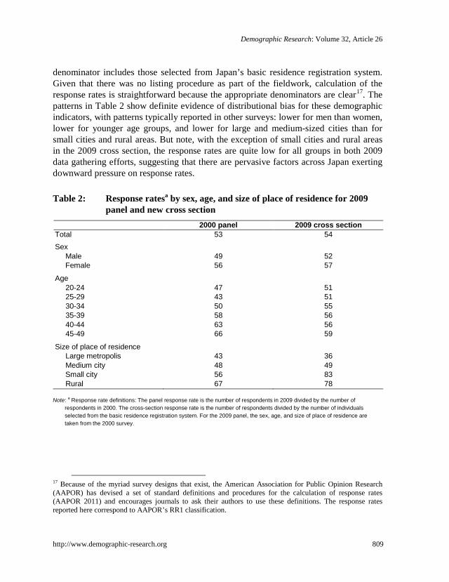
6.1 Response rates by demographic characteristics
Overall response rates as well as response rates by sex, age, and size of place of residence are shown in Table 2. For the 2009 panel the denominator is composed of those who were actual respondents in 2000.16 For the new cross section the
16 The 2000 survey had an overall response rate of 64%. The response rate was particularly low for those aged 20-24 (55%). For the remainder, the response rate was 71%.
Demographic Research: Volume 32, Article 26
http://www.demographic-research.org 809
denominator includes those selected from Japan’s basic residence registration system. Given that there was no listing procedure as part of the fieldwork, calculation of the response rates is straightforward because the appropriate denominators are clear17. The patterns in Table 2 show definite evidence of distributional bias for these demographic indicators, with patterns typically reported in other surveys: lower for men than women, lower for younger age groups, and lower for large and medium-sized cities than for small cities and rural areas. But note, with the exception of small cities and rural areas in the 2009 cross section, the response rates are quite low for all groups in both 2009 data gathering efforts, suggesting that there are pervasive factors across Japan exerting downward pressure on response rates. Table 2: Response ratesa by sex, age, and size of place of residence for 2009
panel and new cross section
2000 panel 2009 cross section Total 53 54 Sex Male 49 52 Female 56 57 Age 20-24 47 51 25-29 43 51 30-34 50 55 35-39 58 56 40-44 63 56 45-49 66 59 Size of place of residence Large metropolis 43 36 Medium city 48 49 Small city 56 83 Rural 67 78
Note: a Response rate definitions: The panel response rate is the number of respondents in 2009 divided by the number of
respondents in 2000. The cross-section response rate is the number of respondents divided by the number of individuals selected from the basic residence registration system. For the 2009 panel, the sex, age, and size of place of residence are taken from the 2000 survey.
17 Because of the myriad survey designs that exist, the American Association for Public Opinion Research (AAPOR) has devised a set of standard definitions and procedures for the calculation of response rates (AAPOR 2011) and encourages journals to ask their authors to use these definitions. The response rates reported here correspond to AAPOR’s RR1 classification.
Rindfuss et al.: Do low survey response rates bias results? Evidence from Japan
810 http://www.demographic-research.org
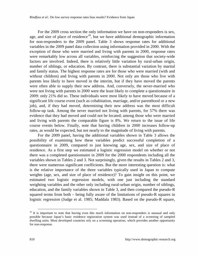
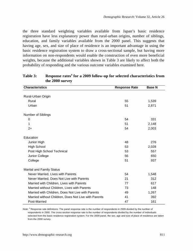
For the 2009 cross section the only information we have on non-responders is sex, age, and size of place of residence18, but we have additional demographic information for non-responders to the 2009 panel. Table 3 shows response rates for additional variables in the 2009 panel data collection using information provided in 2000. With the exception of those who were married and living with parents in 2000, response rates were remarkably low across all variables, reinforcing the suggestion that society-wide factors are involved. Indeed, there is relatively little variation by rural-urban origin, number of siblings, or education. By contrast, there is substantial variation by marital and family status. The highest response rates are for those who were married (with and without children) and living with parents in 2000. Not only are those who live with parents less likely to have moved in the interim, but if they have moved the parents were often able to supply their new address. And, conversely, the never-married who were not living with parents in 2000 were the least likely to complete a questionnaire in 2009: only 21% did so. These individuals were most likely to have moved because of a significant life course event (such as cohabitation, marriage, and/or parenthood or a new job), and, if they had moved, determining their new address was the most difficult follow-up task. Among the never married not living with parents, for 57% there was evidence that they had moved and could not be located; among those who were married and living with parents the comparable figure is 8%. We return to the issue of life course events below. Finally, note that having children in 2000 increases follow-up rates, as would be expected, but not nearly to the magnitude of living with parents.
For the 2009 panel, having the additional variables shown in Table 3 allows the possibility of examining how these variables predict successful completion of a questionnaire in 2009, compared to just knowing age, sex, and size of place of residence. As a first step we estimated a logistic regression model on whether or not there was a completed questionnaire in 2009 for the 2000 respondents including all the variables shown in Tables 2 and 3. Not surprisingly, given the results in Tables 2 and 3, there were numerous significant coefficients. But the more interesting question is: what is the relative importance of the three variables typically used in Japan to compute weights (age, sex, and size of place of residence)? To gain insight on this point, we estimated two logistic regression models, with one just including the standard weighting variables and the other only including rural-urban origin, number of siblings, education, and the family variables shown in Table 3, and then compared the pseudo-R squared terms from both – being fully aware of the limitations of pseudo-R squares in logistic regression (Judge et al. 1985; Maddala 1983). Based on the pseudo-R square,
18 It is important to note that having even this much information on non-responders is unusual and only possible because Japan’s basic residence registration system was used instead of a screening of sampled dwelling units. Most developed countries rely on a screening operation, which provides another opportunity for non-response.
Demographic Research: Volume 32, Article 26
http://www.demographic-research.org 811
the three standard weighting variables available from Japan’s basic residence registration have less explanatory power than rural-urban origins, number of siblings, education, and family variables available from the 2000 panel. This suggests that having age, sex, and size of place of residence is an important advantage in using the basic residence registration system to draw a cross-sectional sample, but having more information on non-respondents would enable the construction of even more beneficial weights, because the additional variables shown in Table 3 are likely to affect both the probability of responding and the various outcome variables examined here. Table 3: Response ratesa for a 2009 follow-up for selected characteristics from
the 2000 survey Characteristics Response Rate Base N
Rural-Urban Origin
Rural 55 1,539 Urban 51 2,871
Number of Siblings
0 54 331 1 51 2,148 2+ 54 2,003
Education
Junior High 48 276 High School 53 2,028 Post High School Technical 53 557 Junior College 56 650 College 51 937
Marital and Family Status
Never Married, Lives with Parents 54 1,548 Never Married, Does Not Live with Parents 21 312 Married with Children, Lives with Parents 77 617 Married without Children, Lives with Parents 73 148 Married with Children, Does Not Live with Parents 49 1,267 Married without Children, Does Not Live with Parents 41 392 Post-Married 47 161
Note: a Response rate definitions: The panel response rate is the number of respondents in 2009 divided by the number of
respondents in 2000. The cross-section response rate is the number of respondents divided by the number of individuals selected from the basic residence registration system. For the 2009 panel, the sex, age and size of place of residence are taken from the 2000 survey.
Rindfuss et al.: Do low survey response rates bias results? Evidence from Japan
812 http://www.demographic-research.org
6.2 Distributional bias
We now turn to the question of whether there is evidence of distributional bias for the more substantive variables of interest (fertility intentions, marital happiness, attitudes, housework, and knowing someone who has engaged in various family or work behaviors). There are 57 such variables. Here we summarize the results. (More details of the variables by tests are displayed in Appendix Table 1.) For the cross section, there are three different variables used in the tests: date the completed questionnaire was picked up, number of visits required to obtain the completed questionnaire, and date by number of visits. For each test-variable by substantive-variable distribution we used a chi-square or analysis of variance (ANOVA) procedure, as appropriate, to see if the distribution of the substantive variable was significantly different across the test-variable categories. Weights based on sex, age, and size of place of residence were used to calculate the distributions. With three test variables and 57 substantive variables, 171 significance tests were performed. Under the assumption of the independence of these 171 tests and using 0.05 criteria for significance, by chance one would expect 9 significant tests. We find that 8 tests indicate significant differences – fewer than expected by chance.
For the panel there is but one test: whether the distribution on the 2000 substantive variable differs between those who responded in 2009 and those who did not, again using a chi-square or ANOVA procedure, as appropriate. Twenty of the 57 tests were significant, including 7 of the 8 household tasks tests. These results are quite different from the cross-sectional results and more in line with work in the labor economics literature on panel studies (e.g., Lillard and Panis 1998; MaCurdy, Mroz, and Gritz 1998). The cross-sectional surveys use the basic residence registration system files as the second stage sampling frame and this system is up to date on address changes. The 2009 panel begins with the 2000 address and then attempts to trace those who have moved. We expect that the difference in distributional bias between the 2009 cross section and panel is the result of differential lost-to-follow-up due to a non-random subset of the 2000 panel having moved and the inability to find some of them. Below in section 6.4 we present circumstantial evidence supporting this. 6.3 Relational bias
For relational bias, our procedure is to estimate a baseline logistic regression, ordered probit or multiple regression as appropriate, where the dependent variable is one of the 57 substantive variables and the independent variables include all 7 demographic and life course variables (sex, age, size of place of residence, number of siblings, rural-
Demographic Research: Volume 32, Article 26
http://www.demographic-research.org 813
urban origin, education, and marriage/family status) and the test indicator19. For the cross-sectional analysis, again there are 3 test indicators (date, number of visits, and date by number of visits) and for the panel analysis there is one (whether successfully followed up or not in 2009). Then, for each of the 7 demographic and life course variables we estimate a model that includes all 7 demographic/life course variables and an interaction between one test variable and the demographic/life course variable using a global significance test,20 that is, testing whether the model with the interaction is a significant improvement over the model without the interaction.
Consider the cross-sectional results first. There are 57 substantive variables by 7 demographic/life course variables by 3 test variables for a total of 1,197 significance tests. Using the conventional 5% cutoff, we would expect 60 significant interactions by chance. We find only 43 significant interactions. Further, as can be seen in Appendix Table 1, for these 43 significant interactions there is no evident patterning by the 57 substantive variables, the 7 demographic/life-course variables, or the 3 test variables.
For the panel, there are 57 substantive variables by 7 demographic/life course variables for a total of 399 interaction tests, and one would expect 20 to be significant by chance. Sixteen were significant. In short, for neither the cross section nor the panel is there substantial evidence of relational bias. 6.4 Life course events and panel retention
Life course events, such as getting married or divorced, can differentially affect the likelihood of response/non-response in the 2009 panel versus the 2009 cross section because: a) changing dwelling units is frequently associated with such life course events; and b) we obtain respondents’ addresses differently in the two data gathering processes. For the 2009 cross section, addresses for those selected to be in the sample are obtained from the basic residence registration system, which is updated within two weeks of a person changing dwelling units. For the 2009 panel we start with their 2000 address, updated if they had responded to periodic requests for address updates. But if they moved without providing a new address we had to track them, asking those at the
19 These regression analyses do not adjust for the cluster design of the sample for two reasons. First, adjusting for the cluster design tends to increase standard errors and thus reduce the likelihood of a significant effect. Since finding few significant effects would be evidence of no relational bias, not correcting for the cluster design is a conservative approach. Second, the survey design was such that there were relatively few respondents per cluster. For example, in the 2009 cross section there were 8.9 respondents, on average, per cluster. In a variety of analyses with these data we find empirically that correcting for the cluster design rarely matters and this is consistent with Monte Carlo simulations on the effect of correcting for cluster design (Guilkey and Murphy 1993). 20 In Appendix Table 1, under the heading “relational tests with interactions”, each cell shows the significance (or insignificance) of one global interaction test.
Rindfuss et al.: Do low survey response rates bias results? Evidence from Japan
814 http://www.demographic-research.org
old address to provide the new address or to forward the questionnaire to the panel member at the new address. So if experiencing a life course event is positively correlated with moving, then the 2009 panel should have a higher likelihood of non-response among those experiencing a life course event than the 2009 cross section, because the basic residence registration system would be more current on address changes.
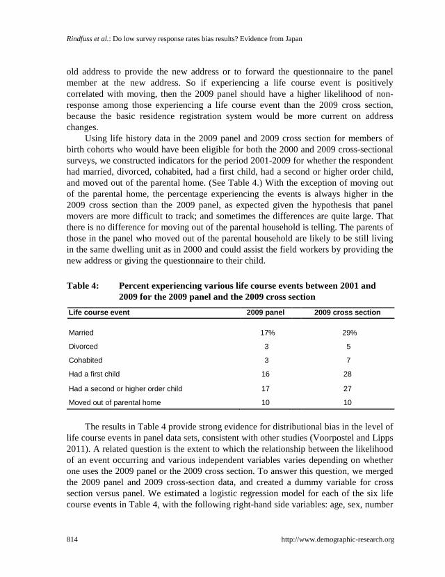
Using life history data in the 2009 panel and 2009 cross section for members of birth cohorts who would have been eligible for both the 2000 and 2009 cross-sectional surveys, we constructed indicators for the period 2001-2009 for whether the respondent had married, divorced, cohabited, had a first child, had a second or higher order child, and moved out of the parental home. (See Table 4.) With the exception of moving out of the parental home, the percentage experiencing the events is always higher in the 2009 cross section than the 2009 panel, as expected given the hypothesis that panel movers are more difficult to track; and sometimes the differences are quite large. That there is no difference for moving out of the parental household is telling. The parents of those in the panel who moved out of the parental household are likely to be still living in the same dwelling unit as in 2000 and could assist the field workers by providing the new address or giving the questionnaire to their child. Table 4: Percent experiencing various life course events between 2001 and
2009 for the 2009 panel and the 2009 cross section Life course event 2009 panel 2009 cross section
Married 17%
29% Divorced 3
5
Cohabited 3
7 Had a first child 16
28
Had a second or higher order child 17
27 Moved out of parental home 10
10
The results in Table 4 provide strong evidence for distributional bias in the level of
life course events in panel data sets, consistent with other studies (Voorpostel and Lipps 2011). A related question is the extent to which the relationship between the likelihood of an event occurring and various independent variables varies depending on whether one uses the 2009 panel or the 2009 cross section. To answer this question, we merged the 2009 panel and 2009 cross-section data, and created a dummy variable for cross section versus panel. We estimated a logistic regression model for each of the six life course events in Table 4, with the following right-hand side variables: age, sex, number
Demographic Research: Volume 32, Article 26
http://www.demographic-research.org 815
of siblings, rural upbringing, and an indicator of cross section versus panel. We then tested for interactions, one at a time, between the cross-section versus panel indicator and the four background variables − a total of 24 interaction tests. Three of the tests were significant: rural upbringing by marriage, rural upbringing and having a first child, and number of siblings and having a second or higher order child. Thus, overall, there is some, but limited, evidence that relationships between the likelihood of an occurrence of a life course event and various independent variables vary depending on whether the 2009 panel or the 2009 cross section is used.
The rural upbringing interactions reinforce the concern that in panel studies higher rates of attrition are associated with life course events. The rural 2009 panel members are the least likely to report having experienced the events, followed closely by urban 2009 panel members. And the rural 2009 cross-sectional respondents are the most likely to report having experienced the events. That the 2009 panel respondents are least likely to experience the events is as expected: panel members who marry and have a child are more likely to move and be lost to follow-up.
7. Summary
In recent years, in Japan and other countries, social support to cooperate with data gatherers has declined, resulting in an increase in non-cooperation by potential respondents. The two 2009 Japanese fieldwork operations examined here had response rates just above 50%, which raises questions about non-response bias, especially in the population research community.
We find that response rates vary substantially by such demographic variables as age, sex, size of place of residence, and especially for the panel by the 2000 marital and family status. But, even more important, non-response is high in all groups with the exception of panel members living with parents in 2000. The patterning of this variation is as one would expect a priori. For the panel, but not the cross section, we also find significant distributional bias for several of the more substantive variables. But when we looked at relational bias, that is, the extent to which the relationship between various independent variables and an array of substantive dependent variables varied by non-response or respondent cooperation, we do not find substantial evidence of relational bias: there were fewer significant interactions than one would have expected by chance.
With respect to experiencing life course events such as marrying or having a child, we find evidence that those who experienced these events were more difficult to follow in the panel, and the likely reason is that they moved and could not be traced. But, again, we find quite limited evidence for relational bias.
Rindfuss et al.: Do low survey response rates bias results? Evidence from Japan
816 http://www.demographic-research.org
8. Discussion
8.1 Our results and common intuition
Our results suggest that potential bias from low response and high attrition rates is less than conventional demographic wisdom would have predicted. Non-response bias is higher for distributional than for relational analyses, and it varies across items within a survey. These findings are consistent with a line of research on attrition in labor economics (Lillard and Panis 1998; Ziliak and Kiesner 1998; van der Berg, Lindeboom, and Ridder 1994; MaCurdy, Mroz, and Gritz 1998; Fitzgerald, Gottschalk, and Moffitt 1998), in the survey research field (Curtin, Presser, and Singer 2000; Groves 2006; Groves and Peytcheva 2008; Groves et al. 2009; Keeter et al. 2000; Keeter et al. 2006; Merkle and Edelman 2002; Peytcheva and Groves 2009), and in a study of nurses (Smith 2009). Results from this nursing study are instructive as an example of a mail-out mail-back survey with a low response rate (27% in California and 39% in Pennsylvania). After obtaining the initial low response rates, Smith selected a small subsample of non-respondents, and used, among other things, financial incentives and a shorter questionnaire to improve response rates. The efforts worked and they had a response rate over 90% in the non-respondent survey. Comparing the low- and high-response surveys, Smith finds no evidence of bias in the low-response survey.
How do we reconcile this growing body of findings that low response rates need not necessarily lead to biased results with our intuition and the perceived common wisdom in the population research community? Beginning with Rubin’s 1976 article, there have been considerable advances in understanding the biases that may be present in analyses of data sets with missing data. Little and Rubin (2002) provide an overview. For our purposes, we point out that many of the statistical procedures for handling missing data rest on the ‘missing at random’ assumption (MAR), which is that data on some variable, Y, are MAR if the probability that Y is missing does not depend on the actual value of Y once a set of X variables is controlled for. Put differently, missingness on Y can depend on a set of observed X variables, but cannot depend on the unobserved (missing) values of Y. The better the relationship between the set of X variables and Y, the less likely it is that bias will be found. So, especially in our relational bias tests, where a variety of X variables are controlled in a regression model, the likelihood is increased that the MAR assumption holds and that unbiased results can be obtained. Since non-response and the kinds of variables used as control variables in regression models tend to be correlated, including control variables in regression models likely reduces, and perhaps eliminates, non-response bias that might otherwise be present (e.g., Fitzgerald, Gottschalk, and Moffitt 1998). And so, logic extended, the more
Demographic Research: Volume 32, Article 26
http://www.demographic-research.org 817
control variables related to non-response that are available, the less likely it is that non-response bias will be present.
There are several implications of our results for population researchers. First, evidence of non-response bias in the distribution of characteristics, behaviors, and attitudes is common, and we need to be careful when reporting distributions from data sources with low or even moderate response rates. Second, evidence of bias in studies examining relationships among variables is uncommon, and we should not automatically assume that a study of relationships using data with a low response or follow-up rate is questionable. Third, if we assume that low response rates will be a feature of survey research in developed countries for the foreseeable future - and this is undoubtedly going to be the case - then checking for response rate bias should be a routine step in data analysis. Further, just because response rate bias was not found when examining one variable in a data set does not mean that it is not present for others in that same data set. Indeed, reviews of non-response bias studies find that there is more variation in bias within surveys than across surveys, that the level of non-response does not predict the likelihood of non-response bias, and that there is no necessary relationship between biases on control variables and substantive variables (Groves 2006; Groves and Peytcheva 2008; Peytcheva and Groves 2009). 8.2 Paradata
One type of data available to those doing survey research and which was used here is paradata, defined as information about the data collection process itself (Bethlehem, Cobben, and Schouten 2011; Couper 1997, 2000; Couper and Lyberg 2005; Wagner 2010). The two paradata variables used above were number of visits required to obtain a completed questionnaire and the date the completed questionnaire was collected. With only a trivial additional cost, many other paradata variables could have been recorded (e.g., Biemer, Chen, and Wang 2013; Couper and Kreuter 2013; Durrant and D’Arrigo 2011; Wagner et al. 2012). West (2013) has shown that paradata in the National Survey of Family Growth is predictive of both response propensity and such population variables as marriage, cohabitation, and fertility. Paradata can be used in the construction of weights (Beaumont 2005; Plewis, Calderwood, and Ketende 2012; Sikkel, Hox, and de Leeuw 2009). Examples of paradata include whether there was a building or neighborhood gatekeeper (a human security guard or some type of electronic gatekeeper); type of structure (such as trailer, single family detached house, and so forth); whether there was a household gatekeeper who had to agree/disagree to provide access to the potential respondent or information on how to reach the potential respondent; whether the potential respondent kept appointments; whether the potential
Rindfuss et al.: Do low survey response rates bias results? Evidence from Japan
818 http://www.demographic-research.org
respondent was offered extra incentives to participate; and the time of day and day of the week of attempted contacts. Additional, potentially relevant paradata would be information on the field worker assigned the case, including basic demographic characteristics (age, sex, marital status, education), past history (years worked as a field worker, response rates in previous surveys, ability to convert initial hesitation of potential respondents to participate), and the field worker’s familiarity with the neighborhood where the potential respondents resides. In addition, field workers can be trained to observe and record aspects of the dwelling unit (Rindfuss et al. 2007).
Further, neighborhood data could be obtained by a variety of methods. In most countries, fine-grain census information is available. Field workers can be trained to record observations about the neighborhood, although there are concerns about the quality of interviewer observations (Casas-Cordero et al. 2013; West 2013). Such observation need not be as detailed as the work of Sampson and colleagues in Chicago (e.g., Sampson and Raudenbush 1999), but field workers could systematically record the amount of litter, presence of graffiti, evidence of abandoned buildings, overall impression of the socio-economic status of the neighborhood, and the extent to which the neighborhood has mixed socio-economic status. 8.3 Extra effort/incentives at the end of fieldwork: An improvement or not?
Survey research organizations have begun to use paradata during the actual data collection process to identify aspects of non-response, build a response propensity model predicting the likelihood that a current non-responder could be converted to a responder, as well as to identify what alterations in the survey protocols might be most successful in the response conversion, sample from non-responders, and then alter the survey protocols to convert non-responses into responses. This approach has been termed “responsive design” (Groves and Heeringa 2006), and the part of the data collection process where the revised protocol is used is the “response phase.” Responsive design is being used increasingly in the U.S., and the question with which we conclude this paper is: what might be the implications of responsive design for non-response bias?
To address this issue we use the example of the U.S. National Survey of Family Growth Cycle 6 (NSFG), conducted March 2002 – February 2003 among women and men aged 15−44, which employed a responsive design approach, and its evaluation in an article by Axinn and colleagues (2011), which shows that the special efforts to convert reluctant respondents affects both descriptive and regression results. NSFG used a screening phase whereby an individual in a sampled dwelling unit is asked to participate in a very short interview to determine whether an eligible respondent resides
Demographic Research: Volume 32, Article 26
http://www.demographic-research.org 819
in the dwelling unit. Thus, there are two points where non-response can occur: screening and recruiting eligible respondents. During the fieldwork, paradata was collected at both the screening and recruiting stages. These paradata were used to produce scores for both types of non-response predicting the likelihood of converting them into respondents, and a sample of non-responders was chosen such that it had a “high mean probability of being interviewed, but including some low probability cases” (Axinn, Link, and Groves 2011: 1131). During the response phase, the following revisions were made in the fieldwork protocols: only the most productive interviewers were used; the use of proxy informants for screening questions was increased; a small incentive for completing the screening was introduced; and incentives for the actual interviews were doubled.
The NSFG regular respondents and responsive-design respondents differ in age, whether working full-time, race/ethnicity, nativity, and education. As would be expected, the two types of respondents differ distributionally on a range of partnership and fertility behaviors. When Axinn and colleagues (2011) interact a regular versus responsive-design variable with various independent variables in regression models that examine a range of demographic dependent variables, they find a substantial number of significant interactions and some cases where the sign changes.
One lesson from the Axinn et al. (2011) study is that analysts using data sets that employ a responsive design need to carefully check whether including cases collected during the response phase alters the substantive results. If the answer is “yes”, then the analyst has to decide which set of results are more likely to be correct. In making this decision it will be important to carefully consider the details of the response phase, and to consider that using enhanced efforts on converting difficult cases may lead to measurement errors in the responses of difficult cases (Fricker and Tourangeau 2010; Olson 2013).
9. Acknowledgements
We thank Robert Retherford and Naohiro Ogawa for data on the response rate trend for Mainichi Shinbun’s National Opinion Survey on Family Planning, and Aat Liefbroer for reponse rates for wave 1 of the Generations and Gender Programme. Discussions with Herb Smith at the start of the analysis were very helpful, as were comments on previous drafts from William Axinn, Ken Bollen, David Guilkey, Martin Piotrowski, Chirayath Suchindran, James Wagner, Brady West, two anonymous reviewers and an associate editor. The analyses reported here were partially supported by a grant from NICHD to the East-West Center (5R01HD042474).
Rindfuss et al.: Do low survey response rates bias results? Evidence from Japan
820 http://www.demographic-research.org
References
American Association, for Public Opinion Research (AAPOR) (2011). Standard definitions: Final dispositions of case codes and outcome rates for surveys. AAPOR.
Atrostic, B.K., Bates, N., Burt, G., and Silberstein, A. (2001). Nonresponse in U.S. government household surveys: Consistent measures, recent trends and new insights. Journal of Official Statistics 17(2): 209−226.
Axinn, W.G., Link, C.F., and Groves, R.M. (2011). Responsive survey design, demographic data collection, and models of demographic behavior. Demography 48: 1127−1149. doi:10.1007/s13524-011-0044-1.
Beaumont, J.-F. (2005). On the use of data collection process information for the treatment of unit nonresponse through weight adjustment. Survey Methodology 31(2): 227−231.
Bethlehem, J., Cobben, F., and Schouten, B. (2011). Handbook of nonresponse in household surveys. Hoboken, NJ: John Wiley and Sons. doi:10.1002/ 9780470891056.
Biemer, P.P., Chen, P., and Wang, K. (2013). Using level-of-effort paradata in non-response adjustments with application to field surveys. Journal of the Royal Statistical Society: Series A 176(1): 147−168. doi:10.1111/j.1467-985X. 2012.01058.x.
Brick, J.M. and Williams, D. (2013). Explaining rising nonresponse rates in cross-sectional surveys. The ANNALS of the American Academy of Political and Social Science 645: 36−59. doi:10.1177/0002716212456834.
Casas-Cordero, C., Creuter, F., Wang, Y., and Babey, S. (2013). Assessing the measurement error properties of interviewer observations of neighborhood characteristics. Journal of the Royal Statistical Society: Series A 176(1): 227−249. doi:10.1111/j.1467-985X.2012.01065.x.
Choe, M.K., Bumpass, L.L., Tsuya, N.O., and Rindfuss, R.R. (2014). Non-traditional family-related attitudes in Japan: Macro and micro determinants. Population and Development Review 40(2): 241−271. doi:10.1111/j.1728-4457.2014.00672.x.
Couper, M.P. (1997). Survey introductions and data quality. Public Opinion Quarterly 61(2): 317−338. doi:10.1086/297797.
Demographic Research: Volume 32, Article 26
http://www.demographic-research.org 821
Couper, M.P. (2000). Usability evaluation of computer-assisted instruments. Social Science Computer Review 18(4): 384−396. doi:10.1177/089443930001800402.
Couper, M.P. and Lyberg, L. (2005). The use of paradata in survey research. In: Proceedings of the 55th Session of the International Statistical Institute, Sydney. Voorburg: International Statistical Institute.
Couper, M.P. and Kreuter, F. (2013). Using paradata to explore item level response times in surveys. Journal of the Royal Statistical Society: Series A 176: 271−286. doi:10.1111/j.1467-985X.2012.01041.x.
Curtin, R., Presser, S., and Singer, E. (2000). The effects of response rate changes on the index of consumer sentiment. Public Opinion Quarterly 64(2): 413−428. doi:10.1086/318638.
Curtin, R., Presser, S., and Singer, E. (2005). Changes in telephone survey nonresponse over the past quarter century. Public Opinion Quarterly 69(1): 87−98. doi:10.1093/poq/nfi002.
De Leeuw, E. and de Heer, W. (2002). Trends in household survey nonresponse: A longitudinal and international comparison. In: Groves, R.M., Dillman, D.A., Entinge, J.L., and Little, R.J.A. (eds.). Survey nonresponse. NY: John Wiley and Sons: 41−54.
Dijkstra, W. and Smit, J.H. (2002). Persuading reluctant recipients in telephone surveys. In: Groves, R.M., Dillman, D.A., Entinge, J.L., and Little, R.J.A. (eds.). Survey nonresponse. NY: John Wiley and Sons: 121−134.
Dillman, D.A., Smyth, J.D., and Christian, L.M. (2009). Internet, mail and mixed-mode surveys: the tailored design method. Hoboken, NJ: John Wiley and Sons.
Durrant, G.B., Groves, R.M., Staetsky, L., and Steele, F. (2010). Effects of interviewer attitudes and behaviors on refusal in household surveys. Public Opinion Quarterly 74(1): 1−36. doi:10.1093/poq/nfp098.
Durrant, G.B. and D’Arigo, J. (2011). Using paradata to predict best times of contact, conditioning on household and interviewer influences. Journal of the Royal Statistical Society: Series A 174: 1029−1049. doi:10.1111/j.1467-985X. 2011.00715.x.
Fitzgerald, J., Gottschalk, P., and Moffitt, R. (1998). An analysis of sample attrition in panel data. The Journal of Human Resources 33(2): 251−299. doi:10.2307/ 146433.
Rindfuss et al.: Do low survey response rates bias results? Evidence from Japan
822 http://www.demographic-research.org
Fricker, S. and Tourangeau, R. (2010). Examining the relationship between nonresponse propensity and data quality in two national household surveys. Public Opinion Quarterly 74(5): 934−955. doi:10.1093/poq/nfq064.
Groves, R.M. (2006). Nonresponse rates and nonresponse bias in household surveys. Public Opinion Quarterly 70(5): 646−675. doi:10.1093/poq/nfl033.
Groves, R.M. (2011). Three eras of survey research. Public Opinion Quarterly 75(5): 861−871. doi:10.1093/poq/nfr057.
Groves, R.M. and Couper, M.P. (1998). Nonresponse in household interview surveys. New York: John Wiley and Sons. doi:10.1002/9781118490082.
Groves, R.M., Singer, E., and Corning, A. (2000). Leverage-saliency theory of survey participation: Description and an illustration. Public Opinion Quarterly 64(3): 299−308. doi:10.1086/317990.
Groves, R.M., Couper, M.P., Presser, S., Singer, E., Tourangeau, R., Acosta, G.P., and Nelson, L. (2006). Experiments in producing nonresponse bias. Public Opinion Quarterly 70(5): 720−736. doi:10.1093/poq/nfl036.
Groves, R.M. and Heeringa, S.G. (2006). Responsive design for household surveys: Tools for actively controlling survey errors and costs. Journal of the Royal Statistical Society: Series A 169(part 3): 439−457.
Groves, R.M. and Peytcheva, E. (2008). The impact of nonresponse rates on nonresponse bias. Public Opinion Quarterly 72(2): 167−189. doi:10.1093/ poq/nfn011.
Groves, R.M., Pressor, S., Tourangeau, R., West, B.T., Couper, M.P., Singer, E., and Toppe, C. (2012). Support for the survey sponsor and nonresponse bias. Public Opinion Quarterly 76(3): 512−524. doi:10.1093/poq/nfs034.
Groves, R.M., Fowler Jr., F.J., Couper, M.P., Lepkowski, J.M., Singer, E., and Tourangeau, R. (2009). Survey methodology. Hoboken, NJ: John Wiley and Sons.
Guilkey, D.K. and Murphy, J.L. (1993). Estimation and testing in the random effects probit model. Journal of Econometrics 59(3): 301−317. doi:10.1016/0304-4076 (93)90028-4.
Hox, J. and de Leeuw, E. (2002). The influence of interviewers’ attitude and behavior on household survey nonresponse: An international comparison. In: Groves, R.M., Dillman, D.A., Entinge, J.L., and Little, R.J.A. (eds.). Survey nonresponse. NY: John Wiley and Sons: 103−120.
Demographic Research: Volume 32, Article 26
http://www.demographic-research.org 823
Inaba, A. (2007). Problems relating to declining response rates to social surveys in Japan: Trends after 2000. International Journal of Japanese Sociology 16: 23−34. doi:10.1111/j.1475-6781.2007.00095.x.
Japanese General, Social Survey (JGSS). Social Science Japan Data Archive. Institute of Social Science, University of Tokyo. http://ssjda.iss.u-tokyo.ac.jp/en.
Judge, G.G., Griffiths, W.E., Hill, R.C., Lutkepohl, H., and Lee, T.-C. (1985). The theory and practice of econometrics. New York: Wiley. doi:10.1017/ S0266466600011294.
Keeter, S. (2012). Assessing the Representativeness of Public Opinion Surveys [electronic resource]. http://www.people-press.org/2012/05/15/assessing-the-representativeness-of-public-opinion-surveys/.
Keeter, S., Miller, C., Kohut, A., Groves, R.M., and Presser, S. (2000). Consequences of reducing nonresponse in a national telephone survey. Public Opinion Quarterly 66(1): 125−148. doi:10.1086/317759.
Keeter, S., Kennedy, C., Dimock, M., Best, J., and Craighill, P. (2006). Gauging the impact of growing nonresponse on estimates from a national RDD telephone survey. Public Opinion Quarterly 70(5): 759−779. doi:10.1093/poq/nfl035.
Lepkowski, J.M. and Couper, M.P. (2002). Nonresponse in the second wave of longitudinal household surveys. In: Groves, R.M., Dillman, D.A., Entinge, J.L., and Little, R.J.A. (eds.). Survey nonresponse. NY: John Wiley and Sons: 121−134.
Lessler, J.T. and Kalsbeck, W.D. (1992). Nonsampling error in surveys. New York: Wiley.
Lillard, L. and Panis, C.W.A. (1998). Panel attrition from the panel study of income dynamics. The Journal of Human Resources 33(2): 437−457. doi:10.2307/ 146436.
Lin, I.-F. and Schaeffer, N.C. (1995). Using survey participants to estimate the impact of nonparticipation. Public Opinion Quarterly 59(2): 236−258. doi:10.1086/ 269471.
Little, R.J.A. and Rubin, D.B. (2002). Statistical analysis with missing data. Hoboken, NJ: John Wiley and Sons. doi:10.1002/9781119013563.
MaCurdy, T., Mroz, T., and Gritz, R.M. (1998). An evaluation of the national longitudinal survey of youth. Journal of Human Resources 33(2): 345−436. doi:10.2307/146435.
Rindfuss et al.: Do low survey response rates bias results? Evidence from Japan
824 http://www.demographic-research.org
Maddala, G.S. (1983). Limited-dependent and qualitative variables in econometrics. Cambridge: Cambridge University Press. doi:10.1017/CBO9780511810176.
Matsumoto, W. (2007). A study on technical and cultural differences in survey methodology between Japan and the United States. International Journal of Japanese Sociology 16: 10−22. doi:10.1111/j.1475-6781.2007.00096.x.
Maynard, D.W., Freese, J., and Schaeffer, N.C. (2010). Calling for participation: Requests, blocking moves, and rational (inter)action in survey introductions. American Sociological Review 75(5): 791−814. doi:10.1177/00031224103 79582.
Merkle, D.M. and Edelman, M. (2002). Nonresponse in exit polls: A comprehensive analysis. In: Groves, R.M., Dillman, D.A., Entinge, J.L., and Little, R.J.A. (eds.). Survey nonresponse. NY: John Wiley and Sons: 243−258.
Mouw, T. and Kalleberg, A.L. (2010). Occupations and the structure of wage inequality in the United States, 1980s to 2000s. American Sociological Review 75(3): 402−431. doi:10.1177/0003122410363564.
Office of Personal Information Protection, Cabinet Office (2006). Act on the Protection of Personal Information. Tokyo: Cabinet Office, Government of Japan.
Olson, K. (2006). Survey participation, nonresponse bias, measurement error bias, and total bias. Public Opinion Quarterly 70(5): 737−758. doi:10.1093/poq/nfl038.
Olson, K. (2013). Do nonresponse follow-ups improve or reduce data quality? A review of the existing literature. Journal of the Royal Statistical Society: Series A 176(part1): 129−145.
Peytcheva, E. and Groves, R.M. (2009). Using variation in response rates of demographic subgroups as evidence of nonresponse bias in survey estimates. Journal of Official Statistics 25(2): 193−201.
Plewis, I., Calderwood, L., and Ketende, S. (2012). Assessing the accuracy of response propensities in longitudinal studies. Survey Methodology 38(2): 167−171.
Rindfuss, R.R., Choe, M.K., Bumpass, L.L., and Tsuya, N.O. (2004). Social networks and family change in Japan. American Sociological Review 69(6): 838−861. doi:10.1177/000312240406900605.
Rindfuss, R.R., Piotrowski, M., Thongthai, V., and Prasartkul, P. (2007). Measuring housing quality in the absence of a monetized real estate market. Population Studies 61(1): 35−52. doi:10.1080/00324720601103858.
Demographic Research: Volume 32, Article 26
http://www.demographic-research.org 825
Rubin, D.B. (1976). Inference and missing data. Biometrika 63(3): 581−592. doi:10.1093/biomet/63.3.581.
Sakamoto, K. (2006). Datsuraku ni kansuru bunseki (sample attrition analysis). The Japanese Journal of Labour Studies 551(June): 55−70.
Sampson, R.J. and Raudenbush, S.W. (1999). Systematic social observation of public spaces: A new look at disorder in urban neighborhoods. American Journal of Sociology 105(3): 603−651. doi:10.1086/210356.
Sikkel, D., Hox, J., and de Leeuw, E. (2009). Using auxiliary data for adjustment in longitudinal research. In: Peter Lynn, P. (ed.). Methodology of longitudinal surveys. Chichester, UK: Wiley: 141−156. doi:10.1002/9780470743874.ch9.
Singer, E. (2006). Nonresponse bias in household surveys. Public Opinion Quarterly 70(5): 637−645. doi:10.1093/poq/nfl034.
Smith, H.L. (2009). Double sample to minimize bias due to non-response in a mail survey. Philadelphia, Pa: Population Studies Center, University of Pennsylvania, PSC working paper series, No. 09-05.
Steeh, C.G. (1981). Trends in nonresponse rates, 1952-1979. Public Opinion Quarterly 45(1): 40−57. doi:10.1086/268633.
Synodinos, N.E. and Yamada, S. (2000). Response rate trends in Japanese surveys. International Journal of Public Opinion Research 12(1): 48−72. doi:10.1093/ijpor/12.1.48.
Tsuya, N.O., Bumpass, L.L., Choe, M.K., and Rindfuss, R.R. (2012). Employment and household tasks of Japanese couples, 1994–2009. Demographic Research 27(24): 705−718. doi:10.4054/DemRes.2012.27.24.
Van der Berg, G.J., Lindeboom, M., and Ridder, G. (1994). Attrition in longitudinal panel data, and the empirical analysis of dynamic labour market behavior. Journal of Applied Econometrics 9: 421–435. doi:10.1002/jae.3950090408.
Vercruyssen, A., van de Putte, B., and Stoop, I.A.L. (2011). Are they really too busy for survey participation? The evolution of busyness and busyness claims in Flanders. Journal of Official Statistics 27(4): 619−632.
Voorpostel, M. and Lipps, O. (2011). Attrition in the Swiss household panel: Is change associated with drop-out? Journal of Official Statistics 27(2): 301−318.
Rindfuss et al.: Do low survey response rates bias results? Evidence from Japan
826 http://www.demographic-research.org
Wagner, J. (2010). The fraction of missing information as a tool for monitoring the quality of survey data. Public Opinion Quarterly 74(2): 223−243. doi:10.1093/ poq/nfq007.
Wagner, J., West, B.T., Kirgis, N., Lepkowski, J.M., Axin, W.G., and Ndiaye, S.K. (2012). Use of paradata in a responsive design framework to manage a field data collection. Journal of Official Statistics 28(4): 477−499.
West, B.T. (2013). An examination of the quality and utility of interviewer observations in the National Survey of Family Growth. Journal of the Royal Statistical Society: Series A 176(part 1): 211−225. doi:10.1111/j.1467-985X.2012.01038.x.
West, B.T. and Olson, K. (2010). How much of interviewer variance is really nonresponse error variance? Public Opinion Quarterly 74(5): 1104−1126. doi:10.1093/poq/nfq061.
Yamada, S. and Synodinos, N.E. (1994). Public opinion surveys in Japan. International Journal of Public Opinion Research 6: 118−138. doi:10.1093/ijpor/6.2.118.
Ziliak, J.P. and Kniesner, T.J. (1998). The importance of sample attrition in life cycle labor supply estimation. The Journal of Human Resources 33(2): 507−530. doi:10.2307/146439.
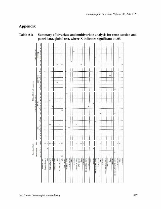
Demographic Research: Volume 32, Article 26
http://www.demographic-research.org 827
Appendix
Table A1: Summary of bivariate and multivariate analysis for cross-section and panel data, global test, where X indicates significant at .05
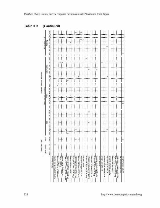
Rindfuss et al.: Do low survey response rates bias results? Evidence from Japan
828 http://www.demographic-research.org
Table A1: (Continued)