Do Reorganization Costs Matter for Efficiency?

Evidence from a Bankruptcy Reform in Colombia

Xavier Giné and Inessa Love*

Abstract

This paper studies the effect of the length of reorganization on the efficiency of bankruptcy laws. We develop a simple model that predicts that in a regime with lengthy reorganizations and thus high reorganization costs, the law fails to achieve the efficient outcome of liquidating unviable businesses and reorganizing viable ones. We test the model using the Colombian bankruptcy reform of 1999. Using data from 1,924 firms filing for bankruptcy between 1996 and 2003, we find that the pre-reform reorganization proceeding was so inefficient that it failed to separate economically viable firms from inefficient ones. In contrast, by substantially lowering the statutory deadline for reorganization, the reform improved the selection of viable firms into reorganization. In this sense, the new law increased the efficiency of the bankruptcy system in Colombia.

JEL: G33 G34 Keywords: bankruptcy reform, reorganization, liquidation, Colombia

_____________________________________________

* Emails: xgine@worldbank.org and ilove@worldbank.org. Both authors are affiliated with the World Bank, 1818 H Street, Washington, DC 20433. We wish to thank Fernando Montes-Negret for sparking our interest in this topic, Enrique Aguirre and the Superintendencia de Sociedades for the data and Rodolfo Danies Lacouture, the Superintendent, for insightful comments on an earlier draft. We also wish to thank Jaime Alberto Gomez, Jorge Pinzón, Felipe Trias and Carlos Urrutia for very useful conversations about the intricacies of the bankruptcy law in Colombia. We finally wish to thank Rei Odawara for excellent research assistance and to Jishnu Das, Asli Demirguc-Kunt, Quy-Toan Do, Leora Klapper, Soledad Martínez Peria, Claudio Raddatz and Kenichi Ueda for valuable comments.

1

I. Introduction

Nearly ninety countries around the world have reformed their bankruptcy codes since

World War II and over half of them have done so during the last decade. The extent to

which these reforms will succeed depends on their design and the context in which the

new codes are binding (Claessens, S., et al., 2001; Franks and Loranth, 2005; Hart, 2000

and World Bank, 2004, 2005 and 2006). Yet, all countries seek to improve the efficiency

of the bankruptcy system by encouraging the reorganization of viable firms and the

liquidation of unviable ones. This requires a delicate balance (White, 1989). On the one

hand, if the law is lenient towards failing firms, it will inevitably allow inefficient firms

to continue operations. On the other, if the law favors liquidation, it will also liquidate

viable firms.

Due to this trade-off, the design of bankruptcy laws is still a much debated topic

(Claessens and Klapper, 2003; Smith and Strömberg, 2004 and references therein). The

debate has focused on comparing two stylized bankruptcy proceedings: cash auctions or

liquidations and structured bargainings or reorganizations. Critics of reorganizations

argue that conflicting interests among claimholders and managers lead to excessively

lengthy and costly negotiations (Baird, 1986; Aghion et al., 1992). Critics of liquidations

claim that they contribute to the inefficient sale of assets due to market illiquidity and

transaction costs (Shleifer and Vishny, 1992; Aghion et al., 1992).1

While there is a growing literature estimating the costs of bankruptcy (Bris et al.

2005 for a review), there is little empirical evidence assessing how these costs affect the

ability of laws to separate viable businesses from unviable ones, a key to ensuring

efficiency. This paper attempts to fill this gap by using a bankruptcy reform that took

place in Colombia.

In the midst of financial crisis, facing a backlog of failing businesses entering a

very inefficient bankruptcy process, Colombia adopted a new reorganization code in late

1999. This law, known as Law 550, streamlined the reorganization process by

establishing shorter statutory deadlines for reorganization plans, reducing opportunities

for appeal by debtors and requiring mandatory liquidation in cases of failed negotiations.

1 Using data from Sweden, Stromberg (2000) show that liquidations also suffer from conflicts of interest among claimholders.

2

We present a simple model that describes the decision to reorganize or liquidate a

financially distressed firm as a function of reorganization costs. In a regime with high

idiosyncratic reorganization costs, some viable businesses may be liquidated if the costs

they face are too high. In this case, the bankruptcy system fails to separate viable from

unviable firms, resulting in inefficient outcomes. In contrast, when reorganization costs

are low, the model predicts that better quality firms are more likely to choose

reorganization, resulting in a clear separation between firms that reorganize and those

that liquidate. In this regime, as a result of both lower costs and better selection, the

recovery after reorganization is significantly improved thus contributing to more efficient

outcomes. The Colombian reform can be seen as a natural experiment with two regimes

that match our model – a pre-reform regime with high reorganization costs and the post-

reform regime with low costs.

We use a unique dataset obtained from the Colombian Superintendence of

Companies which includes a total of 1,924 bankruptcy cases, representing the universe of

cases filed between 1996 and 2004, conveniently spanning the reform episode. We also

use data of about 14,000 active companies that report to the same Superintendence over

the same time period. One attractive feature of the dataset is that it predominantly

consists of non-listed firms thus complementing the US literature, which has focused

mainly on public firms.2 We use data from financial statements and accounting-based

models (e.g. Z-score model of Altman 1968 and 2000) to construct an indicator of

financial distress.

We show that the reform made reorganization an attractive option for distressed

but viable firms. First, we find that the duration of reorganization proceedings

significantly decreases overall and also relative to the duration of liquidations with the

new reorganization code. While data on the direct costs of reorganization do not exist in

Colombia, this finding is in line with our model’s assumption of lower costs after the

reform, since the length of the process is likely to be a major indirect cost of the

2 The literature on reorganization costs in the US mostly draws conclusions from the relatively small number of public corporations (see for example Altman, 1984; Weiss, 1990 and Weiss and Wruck, 1998). A notable exception is Bris et al. (2005), which use a sample of 286 public and private firms, the largest sample in the US, and Davydenko and Franks (2005) who use a large sample of small firms from France, Germany and the UK.

3

reorganization process. Second, under the old law, we observe that firms filing for

reorganization are indistinguishable from those filing for liquidation based on several

measures of financial health. In contrast, relatively healthier (and hence more viable)

firms are more likely to file for reorganization after the new law, producing a clear

separation in the distribution of the two types of firms. Finally, we find that the level of

recovery after the reorganization episode is significantly improved under the new law.

While under the old law firms hovered at about the same low level of financial health for

years after entering into reorganization, we observe a clear recovery under the new law.

We conclude that the new law increased the efficiency of the bankruptcy system in

Colombia.

Previous bankruptcy studies analyze the existing laws of a given country or make

comparisons across different countries. Evidence from the US Chapter 11 reorganizations

offers mixed conclusions on the magnitude of these costs. While Altman (1984) and

Hotchkiss (1995) among others find high Chapter 11 costs, Alderson and Betker (1995)

and Maksimovic and Phillips (1998) find them to be low. More recently, Bris et al.

(2005) show that reorganization costs are heterogeneous across firms but comparable to

US Chapter 7 liquidations costs, although reorganizations as compared to liquidations

preserve the assets better. In contrast, Thorburn (2000) finds that liquidations in Sweden,

which have a statutory deadline, are faster and cheaper than reorganizations in the US.

Bris et al. (2005), however, question the validity of the comparison because the US and

Sweden differ from each other in many other ways besides the bankruptcy codes.

In this paper, we look at the impact of a statutory deadline in the reorganization

proceeding but avoid country comparisons by studying a bankruptcy reform in a country.

We exploit the fact that the reform only affects the reorganization proceeding, allowing

us to compare firms that file for reorganization to firms filing for liquidation before and

after the law. However, since the law was introduced because of a major financial crisis,

we need to make sure that we can attribute the effects to the new law and not the

changing macroeconomic conditions.3 Similarly, a gradual improvement of the judiciary

system could also confound the results. We address these concerns by controlling for

3 See Uribe and Vargas (2002) or Urrutia and Zárate (2001) for details about the causes and magnitude of the crisis.

4

overall trends and making sure that the crisis did not affect differently reorganizations

relative to liquidations. We find that the crisis had the same effect on both groups of

firms, thus suggesting that our identification strategy is valid.

The rest of the paper is organized as follows. Section II develops the model and

Section III outlines the main testable implications. Sections IV and V present and

describe the data in detail. Section VI presents our empirical specifications, Sections VII

and VIII discuss the main results and robustness tests and Section IX concludes. The

background information on the bankruptcy system in Colombia and details of the new

reorganization Law 550 of 1999 are presented in Appendix 1.

II. Model

In this section we develop a model in the spirit of White (1994) that focuses on

the decision to reorganize or liquidate as a function of reorganization costs, which are

specific to the firm (Bris et al., 2005).

A. Assumptions

At date0 , firm i obtains a loan to finance a project that yields an idiosyncratic

return (cash-flow) of at date 1 and at date . The lender (bank) agrees to give the

loan in exchange for repayments

1ix 2ix 2

p at dates 1 and . The repayment schedule is the

same for all firms.

2

If the return from the project at date , , is lower than then firm i is in

financial distress. We follow Kahl (2000) and others and assume that at this point the

bank gains control of the firm and decides whether to liquidate or reorganize the firm. If

liquidation is chosen, the bank obtains

1 1ix p

1ixL + , pL < where L is the scrap value of the

firm's assets. If instead reorganization is chosen, the bank obtains current cash-flow

and allows the firm to continue its operations until date when a new payment will

be made. At date , the value of the firm's assets is zero and the firm is shut down. Thus,

liquidation values at each date are equal for all firms.

1ix

2 2ip

2

Since managers obtain a payoff of zero if the firm is liquidated but may get

“lucky” and receive a positive payoff (net of bank repayment and reorganization costs) if

5

the firm is reorganized, they will always prefer reorganization to liquidation. The bank

however must weight the immediate gain of liquidation against expected net gain of

reorganization.

Letting the firm's net return at date be 2 )()( 222 iiiii xcxxn −= , repayment to the

bank will be 2ip p if net return satisfies but it will only equal net return

if . The cost of reorganization

pxn ii ≥)( 2

)( 2ii xn pxn ii <)( 2 )(⋅ic may include fixed and variable

costs which may depend on the idiosyncratic return itself. But more importantly, as

shown in Bris et al. (2005) for the US and in our empirical results of Section VII.A,

reorganization costs are specific to the firm. Thus, firms may face different expected

reorganization costs at date 1 despite realizing the same returns at dates 1 and .

2ix

2 4 This is

the reason why the cost function )(⋅ic is indexed by . Without loss of generality, we

assume that these costs are bounded above by

i

)( 2ixc . Thus, )()(0 22ix ii xcc ≤≤ . The

only other restriction we impose on these reorganization costs is that the net return

function for firm at date 2 , , be strictly increasing in . i )( 2ii xn 2ix

We assume that there are two types of firms in the economy: economically viable

and unviable firms. A fraction θ of economically viable firms obtain returns x from the

probability density function while unviable (inefficient) firms draw 0),( ≥xxf H x from

the distribution . By definition, the density functions 0),( ≥xxf L HLjf j ,),( =⋅ are such

that , where [ ] [ LpEHpE || 22 > ] [ ] HLjjpE ,,|2 = can be written as

[ ] [ ]∫−

−−+=)(

0

12222

1

))((1)()(|pn

jj pnFpdxxfxnjpE (1)

4 The difference in reorganization costs may come from the specific nature of the firm’s assets or operations, or the bankruptcy process itself, which could carry a large idiosyncratic component, for example, the length of the process could depend on qualifications and experience of a judge or promoter assigned to the case.

6

In addition, we assume that HLjf j ,),( =⋅ satisfy the strict monotone likelihood

ratio property (MLRP).5 With this assumption, the realized return provides

information about the expected return that will be taken into account by the bank

when deciding whether to liquidate or reorganize a distressed firm. In addition, since at

date the bank only knows the proportion of viable firms and loan size is equal for all

firms, the repayment schedule is also the same for every firm.

1ix

2ix

0

Assuming no discounting, the bank will reorganize firm i at date 1 if

[ ] LxpE ii ≥12 | . (2)

Using Bayes Law and dropping subscript i , the expectation in the left hand side

can be written as follows:

[ ] [ ] [ ] [ ] [ ]LpExLHpExHxpE ||Pr||Pr| 212112 +=

[ ] [ ]

)()1()(|)(|)(

11

2121

xfxfLpExfHpExf

LH

LH

θθ −++

= .

where is given by Equation 1. [ ] HLjjpE ,,|2 =

B. Implications

We now discuss the predictions of our model in the context of the Colombian

reform. Since the main purpose of Law 550 was to shorten the statutory deadlines of

reorganizations, we model it as a reduction in the maximum cost from )(⋅Bc (before Law

550) to )(⋅Ac (after Law 550), )()( ⋅>⋅ AB cc . We interpret this cost as the time it takes to

approve a reorganization plan. A potential indirect cost is the time that managers have to

spend in meetings with creditors. Less time involved in actually running the firm may

5 Let xx > , then strict MLRP implies that 0)()()()( >− xfxfxfxf HLLH . See Milgrom (1981) for further details.

7

result in lower cash-flows. Likewise, a prime direct cost is lawyer’s fees, and so the

shorter the proceeding and the less lawyer involvement in a more streamline process, the

lower the expenses should be. As already mentioned, because we do not have data on

direct costs, we use the length of the process as a proxy for theist overall cost.

Figure 1 explains in a graph the decision that banks face at date by plotting the

payoffs to liquidation and reorganization in Equation 2 in the relevant range of observed

cash-flow at date 1, , when the firm is in distress,

1

1ix pxi <1 . The liquidation value is the

same in both panels because only reorganization was affected by the change in the law.

The expected payoff to reorganization can be written as:

⎩⎨⎧ <

=otherwise,

if ]|)([]|[ 112

12 pxxxxnE

xpE ipiiiiii

where is defined as the observed cash-flow at date 1 that makes the net

expected payoff to reorganization equal to

ipx

p .6 Given the assumption of MLRP, expected

net cash-flow at date is increasing in observed cash-flow at date 1, . For a

firm that expects reorganization costs to be zero, expected net cash-flow for a distressed

firm equals that of an active firm and is simply the expected cash-flow itself. This is

given by the top increasing line as

)( 2ii xn 2 1ix

2ix

1x goes from 0 to , and the horizontal line at

for . Since cash-flows are not affected by the law, the payoff to reorganization for

firms that expects zero costs is the same (as shown in the left and right panel of Figure 1).

The key difference arises when expected reorganization costs are positive. The bottom

increasing line from to plots expected net cash-flow for a firm that expects

the maximal reorganization costs. As described above, these expected costs are higher

before the law (left panel) than after (right panel).

px p

pxx >1

0 p )( 2ii xn

6 More formally, is such that . Notice that could be higher, equal or lower than .

Since reorganization costs only matter if the firm is in financial distress, that is, when cash-flows at date satisfy , if the threshold is such that , then is irrelevant. This is the case in both panels of Figure 1 when expected reorganization costs are maximum. However, in the example of Figure 1, when expected reorganization costs are zero we have that and thus appears in Figure 1.

ipx pxxnE ipii =]|)([ 2 ipx p

1px i ≤≤ 10 ipx pxip > ipx

px ip < ipx

8

Because costs are specific to the firm, a firm in distress before the law with a

relatively high cash-flow could be liquidated if the expected reorganization costs were

high, while a firm with a low cash-flow could be reorganized if the expected

reorganization costs were low. In other words, depending on the distribution of expected

reorganization costs across firms, the distribution of cash-flows between firms that

restructure and those that liquidate before the law could be the same. In this case, the law

induces reorganization costs that are so high that prevent firms with relatively high cash-

flows (most likely economically viable firms) from reorganizing.

After the law is introduced, however, reorganization costs decrease substantially.

There is a threshold cash-flow at date 1 , , such that if date 1 cash-flow satisfies

, then it is never optimal to liquidate even if the firm expect the maximum

reorganization costs. Firms with may still be either liquidated or reorganized,

depending on the expectation of

*x*

1 xx >

*1 xx <

)(⋅ic . As a result, liquidated firms will tend to have

lower cash-flows than reorganized firms.7 After the reform, reorganization costs are

lower, so banks prefer to always reorganize firms with relatively high cash-flows. In

essence, the bankruptcy system is able to separate and rehabilitate firms that are expected

to be viable from those that are not.

C. Discussion

The model just described is very stylized but does deliver the prediction that if

costs are large enough, the bankruptcy law may fail to achieve one of its prime

objectives: the screening of viable firms from unviable ones. Simplicity however comes

at the cost of abstracting from potentially important issues. For example, it has only one

creditor, like in Kahl (2002), so we do not model coordination frictions among creditors,

as in Bulow and Shoven (1978), Gertner and Scharfstein (1991) or Strömberg (2000). We

7 Figure 1 is drawn assuming that the expected repayment to the bank when the firm does not expect reorganization costs (or expects net cash-flow ) is higher than its liquidation value even if the firm obtained zero cash-flow at date . If this assumption does not hold, then firms with very low cash-flow would always be liquidated, before and after the reform. It would still be the case that in the high cost regime (before Law 550), firms with relatively high cash-flows could still be liquidated if reorganization costs expected by the firm were large enough.

2x

1

9

also abstract from ex-ante efficiency discussions, as we only focus on the decision to

reorganize or restructure once the firm is in financial distress.

The model however can easily be extended to a setup similar to Kahl (2002) to

explore another dimension of efficiency in bankruptcy laws. Kahl (2002) presents an

interesting model where in the context of uncertainty about the firm's viability, a strategy

of delayed liquidation where the firm is allowed to continue but is kept highly leveraged

may be desirable, as it allows creditors to observe future firm performance and to make a

better informed decision. In our model of heterogeneous and uncertain reorganization

costs, banks could regret having reorganized firms that ex-post ended up with a large cost

of reorganization. If at date 1 distressed firms were allowed to continue producing

without incurring reorganization costs but actual reorganization cost were still realized at

date , then if banks were given another chance to choose between liquidation and

continuation, they would in some cases revert their decisions and force firms to a

mandatory liquidation. The likelihood of this event depends on how large the

reorganization costs can be. Because reorganization costs are significantly lower after the

reform, the number of reorganization cases that end up in mandatory liquidation should

be lower. We test this prediction below.

2

Finally, the model assumes that liquidation values and the distribution of cash-

flows remain unaffected by the introduction of the law. But because the law is introduced

during a major crisis, one could make the argument following Shleifer and Vishny (1992)

that adverse macroeconomic conditions may lower liquidation values (as well as the

distribution of cash-flows). This is particularly important in the context of the model

because the result of separation of viable and unviable firms obtained from a relative

improvement of reorganization costs could also come from lower liquidation values.8 We

offer a test of this assumption below.

III. Testable Assumptions and Implications

8 Changes in the distribution of cash-flows are analogous to changes in reorganization costs. A worsening of the distribution of cash-flows (as an increase in reorganization costs) will result in more liquidations and thus will work against the separation of viable from unviable firms.

10

This section describes the testable assumptions and implications of the model that

follow from the introduction of the new law: (A) reduction in reorganization time, (B)

selection of healthier firms into reorganization, and (C) faster recovery of reorganized

firms.

The results are driven by two different types of firms: those that would have filed

for reorganization under both laws, and those that would not file under the old law (either

because they filed for liquidation or were involved in out-of-court settlements) but now

file under the new reorganization proceeding. We consider them together in the analysis

of Section VI.

A. Duration of Reorganization

In light of our model, we interpret the effect of Law 550 as a decline in

reorganization costs. One obvious component of the overall cost of reorganization is the

time it takes to approve the reorganization plan (Franks and Torous, 1989 or more

recently Bris et al., 2005). Since the new law limited the negotiations to a maximum of

eight months, one would expect total costs (direct and indirect) to also decrease on

average. Due to absence of data on direct costs of reorganizations, we use duration of the

process as our proxy for the costs.

Hypothesis A1. The duration of reorganization decreases after the new law is

introduced (overall and relative to liquidations).

The model assumes that liquidation values did not change. Since we use duration

as a proxy for costs, we test this assumption by using indirect liquidation costs (measured

by the duration of liquidations) as a proxy for liquidation value: 9

Hypothesis A2. The duration of liquidation remains constant, and thus liquidation

values do not change.

To test the validity of these hypotheses, we compare the length of reorganization

and liquidation cases before and after the law.

9 Liquidation values could also be driven by the fluctuations in the scrap value of the assets that are uncorrelated with the costs of liquidation as measured by the length of the process. We don’t have adequate data to test this assumption.

11

B. Selection into Reorganization

The main implication from the model is that the reform contributed to the

efficiency of the bankruptcy law by separating viable from non viable firms. Before the

law, reorganization was so inefficient that it failed to separate viable from unviable firms.

Here we test whether the new Law 550 improved the efficiency of the bankruptcy system

by allowing viable firms to choose reorganization as a now attractive alternative.

Hypothesis B1. Before the new law, liquidating firms are indistinguishable from

reorganizing firms, while after the law, liquidating firms have weaker financial health,

relative to reorganizing firms.

Also as discussed in the previous section, the resulting efficiency of the

reorganization procedure should result in a lower proportion of reorganization cases that

end up in mandatory liquidation.

Hypothesis B2. The number of reorganizations that result in mandatory

liquidation is lower after the new law.

C. Recovery after Reorganization

As a direct result of both lower costs and better selection, the recovery of

distressed firms after reorganization should improve significantly.

Hypothesis C. Reorganized firms recover faster after the new law.

IV. Data

The data used come from the Superintendence of Companies of Colombia. We

use two different datasets, bankruptcy filings and financial statements. We now explain

each one in more detail.

A. Bankruptcy Data

These data include the universe of liquidations (L) and reorganizations (R) filed

with the Superintendence from 1995 until 2004. R firms are divided into Concordato and

Acuerdo, depending on the time of the filing. Before 2000 (under Law 222), the firm

filed a Concordato, while after 2000 (under the Law 550), it filed an Acuerdo.

12

All cases report the starting date but only about half report the ending date. Many

of the ending dates are missing because the process is still ongoing, especially among

liquidations.10 For firms that have a start and end of the filing, we construct a

DURATION variable that measures the length of the proceeding in months.

Since reorganization automatically ends in mandatory liquidation if negotiations

break down, in many cases the same firm files first for reorganization and later for

liquidation. In our analysis, we only use data of the firm’s initial filing. Thus, if the firm

first applied for reorganization and then was forced to liquidate, we only use data from its

reorganization. While this shortens our liquidation sample by about half of the total

number of liquidations observed, this rule ensures that all firms enter liquidation directly,

and not as a result of failed reorganizations.

Table 1A reports the distribution of firms that entered bankruptcy proceedings

under each of the three cases. We have a total of 1,924 initial filings. About a quarter of

these firms file for liquidation directly and the rest of file for reorganization. About half

of our sample filed under the old law.

In addition to initial filings, Table 1A also reports the total number of mandatory

liquidations in the second column. A total of 214 firms that originally filed a Concordato

and 184 firms that filed an Acuerdo have later on filed for liquidation.11 As discussed

above, all these secondary filings are excluded from analysis. This allows us to focus on

the initial filing decision, which we believe is the most affected by the legal reform.

B. Financial Data

In addition to firms that filed for liquidation or reorganization, we have data for

all firms that periodically report to the Superintendence of Companies. By law, all firms

with sales or assets exceeding 6,000 minimum wages in the fiscal year, foreign branches,

commercial consortiums, livestock funds and special interest firms as declared by the

president are required to provide financial statements once a year to the Superintendence.

10 We found 13 Concordato cases with a recorded starting date after 2000. Since the new law was passed in December 1999, there should be no Concordato cases after 1999. We therefore drop these 13 cases from our sample. 11 In addition, 50 firms that filed a Concordato under the old law, later filed an Acuerdo under the new law (not shown in Table 1A). Of these cases, 21 failed and moved to mandatory liquidation.

13

Our sample consists then of larger firms although virtually none is listed in the

Colombian stock exchange. Table 1B reports the sector breakdown. The data cover the

period 1996-2003 and contain about 14,000 firms with close to 70,000 firm-year

observations. We refer to this as the sample of active firms.

We merged our sample of bankrupt firms with the financial data sample using a

firm unique identifier. Out of 1,924 bankrupt firms only 1,201 firms have financial data

in at least one year, resulting in a total of about 5,400 firm-year observations. Our panel

is rather unbalanced and for many firms we only have one or a few years of data

available; some firms have only pre-filing data and some have only post-filing data. The

last three columns of Table 1A give the distribution of these firms with financial data

across three types of proceedings and initial time of the filing.

For our bankrupt firms we create a timeline around the time of filing. We refer to

the year of filing as year 0, the first year after filing as +1 and the year before filing as -1.

To study the filing decision, we would like to use financial data at the time of

filing (i.e. year 0). However, for some firms we have no data for the filing year, but have

some data from previous years.12 To increase our sample size we use all firms that have

data for either year 0, -1 or -2. In total, we have 1,032 bankrupt firms with pre-filing

financial data. We refer to this as the bankrupt sample.

In addition to the filing decision, we are interested in comparing the speed of

recovery after filing for reorganization before and after the new law. To do this we

require pre and post filing data. To ensure that observed changes in performance are not

caused by changes in sample composition, we construct a sample of firms with available

financial data for the filing year and at least one year pre and post filing. Due to this

stricter data requirement, we have only around 300 firms with about 2,000 firm-year

observations. We refer to this as our time-series sample.

C. Matched Sample of Active Firms

12 For example, we have 794 firms with data for the filing year. In addition, we have 166 firms with financial data for year -1 (but no data for the filing year) and additional 73 firms have data for year -2 (but no data for year 0 or -1).

14

Our filing data include years with different macroeconomic conditions, including

an episode of major financial crisis in 1999. To control for differences in macroeconomic

conditions affecting our bankrupt firms, we create a matched sample of active firms. For

each firm in our bankrupt sample we pick one active firm that matches the bankrupt firm

by size, year and industry. First, we pick all active firms in the same industry and same

year as the bankrupt firm.13 Then, for each bankrupt firm we find an active firm (among

all active firms available in the same year and industry) that is closest in absolute distance

to the size of the bankrupt firm, based on total assets. We make sure that the same active

firm is not assigned to two different bankrupt firms in different years. We end up with

1,032 matched (M) firms (one for each firm in our bankrupt sample), referred to as the

matching sample.

D. Variables

We focus on several financial characteristics of the firm. On the liability side, we

calculate the following indebtedness ratios: total liabilities, trade credit and total debt, all

scaled by total assets (we refer to these ratios as TL_TA, TRADE_TA and DEBT_TA,

respectively). We also look at two performance ratios: ROA – return on assets, calculated

as income before taxes over total assets and RE_TA - the ratio of retained earnings over

assets. The former reports the performance of the firm in the year prior to the filing and

the latter reflects cumulative performance over time, i.e. firms that continually have been

making losses will have low (or even negative) retained earnings.

Our main firm characteristic is the Z-score index constructed by Altman (1968)

and updated by Altman (2000). It combines indebtedness, performance and liquidity

measures and is commonly used as an indicator of financial distress.14 Based on Altman

(2000) model estimated for non-publicly listed firms, the Z-score is given by:

13 Thus, if a bankrupt firm has data for year 0, we use that year to find a match, but if it has financial data for year -1 or -2, we use that year to find a match. 14 Although recent research has challenged the use of accounting-based models such as Altman’s in favor of Black-Scholes-Merton default probability models (Hillgeist et al., 2004), these models require stock market data. Unfortunately, most of the firms in our sample are non-listed firms. But even if we had stock market data, it remains to be settled whether the stock market in Colombia is efficient, as BSM default probability models assume. In any event, rather than using the Z-score to predict actual default, we use it a measure of firm financial health in order to assess the impact of the law.

15

Z-score=0.717*WC_TA + 0.847*RE_TA+ 3.107*ROA+ 0.420*BVE_TL+0.998*S_TA

where, WC_TA is working capital (defined as current assets minus current liabilities over

total assets), which is a measure of liquidity, ROA and RE_TA are describe above,

BVE_TL is the ratio of book value of equity over total liabilities (a measure of

indebtedness similar to the ratio of total liabilities to total assets) and S_TA is a ratio of

total sales over total assets, which is used as another performance measure. We report the

results for the composite Z-score, as it presents the overall measure of financial health. In

most cases, since the sub-components of the Z-score behave similarly to the overall

measure, the results are not reported (but are available on request). Finally, we use firm

size (calculated as log of total assets) and firm age as controls.

To eliminate influential observations, we clean the data and remove outliers on all

ratios. For ratios that are bounded from below by zero we only remove 1% of outliers on

the top. For unbounded ratios we remove 1% on the top and the bottom of the

distribution.15 For Z-score we remove outliers for each individual component before

constructing the Z-score.

Table 1C reports basic summary statistics for our two samples of bankrupt firms

and matched firms. As Table 1C shows, there is no difference in size and age between

bankrupt and matched active firms.

V. Descriptive Analysis

In this section we present graphical evidence and univariate mean tests. Figure 2

plots kernel density distributions of the Z-score for R (reorganizations), L (liquidations)

and M (matched active firms) before and after the change in the law. The vertical lines

indicate the mean of each distribution.16 As Figure 2 shows, before the new law was

15 The exception is the return on assets, for which we remove 2% on the top and bottom ends because this variable has very long tails. In addition, for our time-series tests we remove outliers before and after constructing the matched sample. 16 Although the model derives testable implications from the firm returns, we use the Z-score index as both are related. Return on assets (ROA) is a component of the overall Z-score index.

16

introduced, R and L firms have very similar density distributions of Z-scores. Thus, firms

filing for reorganization were not significantly different from the firms filing for

liquidation. However, after the new law was introduced, the differences in the

distributions of R and L firms become more pronounced. Firms that liquidate are now

clearly weaker relative to firms that reorganize. The whole distribution of L-firms shifted

to the left with the new reorganization proceeding. In addition, the sample of matched

active firms seems better off as its kernel density distribution has moved slightly to the

right as compared to before the law. This presents the first evidence in support of

Hypothesis B1.

We further examine the data using univariate mean tests of the variables described

in Section IV.D. We first make pair-wise comparisons before and after the law

(comparing R to L firms, R to M firms and L to M firms) and later we make before and

after comparisons for each firm category. Tables 2A and 2B present the results.

Several patterns seem to emerge from the data. Not surprisingly, columns 5 and 6

of Table 2A show that R and L firms are significantly different from M firms: they have

higher levels of debt (including bank debt and trade credit debt) and lower performance.

Their overall financial health, measured by Z-score, is significantly weaker. In fact,

active firms have on average positive Z-scores, while bankrupt firms have negative Z-

scores.

The most interesting result comes from the comparison between R and L before

and after the law. In column 4 of Table 2A we see that R firms are not significantly

different from L firms before the law based on all six characteristics reported. However,

from column 10 we see that R firms are significantly different from L firms after the law

in five out of six characteristics. R firms have lower levels of total liabilities and trade

credit obligations (and lower, but not statistically different levels of bank debt), better

operating performance and higher overall Z-scores. These results confirm the graphical

evidence of Figure 1 and provide additional evidence in support of Hypothesis B1.

17

Table 2B presents a different cut of the data.17 We again find that L firms are

significantly worse after the law, having more debt and lower performance on all

measures.

Finally, the duration of both liquidations and reorganizations is shorter after the

new law. The difference is much more pronounced for reorganizations, from an average

of 34 months before the law to 12 months after. The difference for liquidations is more

modest, with a change from 49 to 33 months. Recall however that duration can only be

computed if both start and end dates are available. Since liquidations are usually long, our

sample of finished liquidations is biased towards relatively short liquidations, especially

after the law was introduced. We explore these differences more rigorously in Section

VII.A.

VI. Regression Models

In this section we present the econometric models used to test formally the

assumptions and implications of the model described in Section III. All models compare

reorganizations to liquidations before and after the law. In some specifications we include

the sample of active firms.

A. Duration of Reorganization

We are interested in comparing the length of reorganization and liquidation cases

before and after the law. The model we use is given by:

Durationi = β1Afteri + β2Ri+ β3Afteri* Ri + Xi’γ + ei, (2)

where After is a dummy equal to one if the filing date occurred after the new law,

R is a dummy for firms filing for reorganization and vector X contains control variables

like firm age and size.

17 Although the means presented in this table are the same as those reported in Tables 2A, we compare here firms in the same category (R, L and M) before and after the law.

18

Since half of the cases lack the end date, we assume that these cases are still

unfinished.18 To properly account for these unfinished cases, we estimate a Cox

proportional hazard model. Coefficients in the hazard model of Equation (2) that are

larger than one and significant are to be interpreted as increasing the probability that

cases will end. Therefore, variables associated with positive and significant coefficients

will contribute to shorter durations. The coefficient β1 shows the effect of the new law on

the length of liquidations and therefore tests Hypothesis A2. It should be insignificant.

Coefficient β2 picks up the average difference in the duration between reorganization and

liquidations before the law. Finally, β3 picks up the length of reorganization as compared

to liquidations after the law, and if Hypothesis A1 is correct, it should be positive and

significant.

B. Selection into Reorganization

We estimate the following model combining the sample of bankrupt firms with

the matched sample of active firms:

Yi = β1Afteri + β2BBi+ β3Afteri* Bi + β4BiB

*Ri + β5Afteri*Bi*Ri + Xi’γ +ei (3)

Here Y is one of the 6 dependent variables described in the previous section. In

addition, B is a dummy for bankrupt firms (i.e. this dummy is equal to one for either R or

L firms). We estimate these models by OLS, with heteroskedasticity-adjusted (White)

standard errors.19

In this specification, β1 shows the effect of the new law on active companies, β2

shows the difference between bankrupt and active firms before the new law, β3 shows the

difference between bankrupt and active firms after the new law, β4 shows the difference

between R and L before the new law and β5 shows the same difference after the new law.

18 The latest closing date in our data is August 3, 2004. 19 Note that B*R dummy is the same as R (in that R firms are included in B category), but we present it in the form of interaction to highlight that in this model we not only compare firms that reorganize (R) to those liquidate (L) among bankrupt firms but we also compare bankrupt firms to active firms.

19

The coefficient of interest is β5, the differential impact that the new law had on R versus L

firms.20

C. Recovery after Reorganization

Finally, we want to test whether the new law contributed to a faster recovery of

reorganized firms. Naturally, we do not have any post filing data for liquidation cases.

Presumably these firms closed down or at least ceased to produce financial statements.

Thus, this analysis is done only using reorganization cases. As already mentioned in

Section IV.B, the sample for this analysis is smaller because of limited pre and post-law

data availability.

Again, we focus on the Z-score as our main indicator. We expect to obtain

something similar to a V-shape: a declining pattern before the filing as financial health

deteriorates, and an increasing pattern (i.e. recovery) after the filing. We are interested to

see whether this shape is affected by the law reform. Thus, we are interested in the slopes

of time-trend variables. We define two time-trend variables: pre-filing period (Pretrend)

and post-filing period (Posttrend). The Pretrend variable takes values -1, -2, -3 for years

before the filing (and zero otherwise) and Posttrend variable takes value 1 in the year of

filing, value of 2 in the first year after the filing and so on.21

Since the law was passed in 1999, the worst year of the crisis, firms filing after

the law face an expansionary period while those that filed before the law faced the

contraction. Thus, the effect of the overall macroeconomic conditions could be

confounded with the effect of the new law that we are trying to capture. To remedy this

problem, we assume that both bankrupt and active firms are equally affected by the

macroeconomic conditions (an assumption that we are able to test in the next section).

Our dependent variables are therefore defined as the difference in Yit between bankrupt

and matched active firm. The model is given by

20 We also run two simpler models: the first compares bankrupt firms with active firms, i.e. in effect restricting the model to β1, β2 and β3. The second model compares R to L firms, limiting the sample to include only bankrupt firms and thus only estimating β1, β4 and β5. The results are similar and not shown but available upon request. 21 We also experimented with defining post-trend starting in the year after the filing (instead of the year of the filing) and including separate dummies for the filing year and we obtained similar results.

20

DiffYit = β1Afteri + β2Pretrendit+ β3Postrendit+ β4Afteri* Pretrendit + (4)

β5Afteri*Postrendit+Xi’γ +eit.

In this model, β2 shows the slope of DiffYit for years preceding the filing for firms

that filed before the law. Analogously, β3 shows the slope of DiffYit for the years after the

filing again for firms that filed before the law. We expect β2 to be negative (i.e. Z-scores

decreasing over time) and β3 to be positive if the firms recovers after the reorganization.

The interaction of trends with the After dummy will show differences in pre and post

trend slopes for firms filing after the new law relatively to the slopes on these trends for

firms filing under the old system.

VII. Regression Results

A. Duration of Reorganization

Table 3 reports the hazard ratios from the Cox proportional hazard model in

specification (2). In Column 1 the whole sample of firms for which we have duration data

is used. Column 2 reports the same regression as Column 1 estimated on the sample of

firms with financial data. The rest of columns include additional controls.22

We find that the AFTER coefficient is not significant in any specification. This

implies that there are no differences in the length of liquidations before and after the law

as Hypothesis A2 suggests. Second, reorganization proceedings seem to have shorter

duration, especially after the reform. Before the reform, the marginal probability to finish

the reorganization process (at any point in time) is 3 times that of the probability to finish

liquidation. However, after the new law, this difference jumps to 14-25 times (depending

on the specification). These results provide strong evidence that the law reform was very

effective in shortening the length of reorganization, as Hypothesis A1 suggests.

22 The number of observations is 1,896. The total number of bankrupt firms is 1,924 as shown in Table 1A. A total of 28 observations are dropped either because the start date is missing or the end date comes before the start date.

21

The last specification explores the relationship between duration and Z-score at

the time of filing. We find that while the length of liquidation does not depend on initial

Z-score, healthier firms have shorter reorganizations. This effect is stronger (about twice

as much) after the law. In terms of the equations depicted in Figure 1, this finding

suggests that the expected net cash-flows for the firm that expects the maximum

reorganization costs (bottom increasing line as goes from 0 to p) has higher slope than

expected cash-flow from 0 to p (upper increasing line as goes from 0 to p). Before the

law this effect is smaller than after the law.

1x

1x

B. Selection into Reorganization

Table 4 reports our baseline results of the specification given in (3) which

analyzes the financial conditions of firms at the time of filing. We focus our discussion

on the Z-score results reported in Column 6. Bankrupt firms have significantly lower Z-

scores relative to active firms as the coefficient on the B dummy is negative and very

significant, with a t-statistic of 9.7. This difference between bankrupt and active firms is

even more pronounced after the new law as evidenced by the coefficient on After*B that

is negative and significant. At the same time, the After coefficient suggests that active

firms appear in better shape after the new law.

The coefficients of interest are the interactions B*R and After*B*R. The first one

is not significant, suggesting that under the old law there was no significant difference

between firms filing for reorganization (i.e. R firms) and the firms filing for liquidation

(i.e. L firms). However, the triple interaction is positive and significant at 1%, suggesting

that under the new law there is significant difference between L and R firms and that R

firms have higher Z-scores relative to L firms. In other words, after the new law R firms

are significantly healthier relative to L firms. These results confirm those obtained in the

graphical analysis and mean tests and support our Hypothesis B1.

We observe similar patterns in other dependent variables, although significance is

somewhat weaker than the overall Z-score measure. The coefficient on the triple

interaction is significant for ROA, RE_TA, and for LIA_TA (at 11%). These results

provide strong evidence for the effectiveness of the new law in separating healthier firms

for reorganization.

22

We also compare the number of reorganizations that result in mandatory

liquidations before and after the new law. Table 1A shows that about 40 percent of firms

filing for reorganization under the old law ended up in liquidation, while only about 26

percent did so under the new law. This difference is statistically significant with a t-

statistic of close to 6. This result, validating Hypothesis B2, is further evidence that Law

550 contributed to the efficiency of the Colombian bankruptcy system.

C. Recovery after Reorganization

Finally, we study the time-series patterns in the Z-score for reorganizing firms.

Note that our sample for this test contains firms with at least one pre-filing data point and

at least one post-filing data point. Table 5A reports the average Z-scores for firms filing

before and after the law and Figure 3 plots these means on a graph. We observe a clear

pattern of declining Z-scores before filing, as expected. The financial health deteriorates

as firms get closer to the verge of insolvency. This declining pre-filing pattern is

observed for firms filing before and after the law. However, the recovery patterns are

quite different in the two regimes. Before the law, no clear recovery is observed. Firms

that filed for reorganization, if anything, are getting worse. In contrast, the recovery is

very pronounced after the introduction of Law 550, with a clear upward trend in the years

following the filing.

Table 5B presents the regression analysis corresponding to the graphical evidence

just described. As expected, the Pretrend coefficient is negative for performance

measures (ROA and RE_TA) and positive for leverage measures, suggesting that before

the filing, leverage is increasing while performance is deteriorating. There is no

significant difference in pre-trend patterns before and after the law. However, there is a

significant difference in the Posttrend after the new law – the coefficient is positive and

significant for the Z-score (but insignificant for individual measures). We consider the Z-

score results to be the most important as this measure represents the overall index of

financial health. These results suggest that after the new law, the reorganization process

results in a more pronounced recovery in the years following the filing. This is in stark

contrast to the post-filing pattern under the old law, which showed a continuous

deterioration in firm performance. This evidence validates our Hypothesis C.

23

VIII. Robustness to Crisis and Trend

As mentioned in the introduction, the new law was introduced in the midst of a

major financial crisis in late 1999. For our identification strategy to work, we need to

make sure that the crisis did not have a differential effect on R relative to L firms.

Otherwise, the effects we observe after the introduction of the law could also be due to

the crisis itself. We test this by creating two crisis windows: year 1999 (the worst year of

the crisis) and years 1998-2000, which span the worst crisis year. Fortunately, since our

sample covers 1996-2003, we have several years outside of the crisis window on both

sides (before and after the law), which allows us to test whether our results are influenced

by the crisis.

Another potential concern with our results is that the effect that we attribute to the

law reform could actually come from a gradual improvement in the efficiency of the

bankruptcy system over time. To test that we create a linear time trend and use it in

interactions in the same fashion as our After variable.

The crisis and trend regressions are presented in Table 6A for our duration results

and Table 6B for Z-score.

In both tables, the first column reproduces the baseline specification for

comparison: in Table 6A it is model 1 from Table 3 and in Table 6B it is model 7 from

Table 4. Model 2 adds the trend and its interactions, Model 3 adds Crisis99 and its

interactions, Model 4 adds Crisis98_00, Model 5 adds Crissis99 and trend and Model 6

adds Crisis98_00 and trend.

Our main interactions with After*R (Table 6A) and After*B and After*B*R (in

Table 6B) remain significant in all the specifications, suggesting that the difference

between the pre-reform and post-reform periods is not related to the financial crisis.

In Table 6B we see that Crisis99 dummy is significant and negative, suggesting

that all firms were worse off during 1999, but Crisis98_00 is not significant, so the worst

of the crisis is limited to 1999. Neither Crisis*B, nor Crisis*B*R interactions are

significant, suggesting that crisis did not have any differential effect on bankrupt firms

(relative to active) or R firms relative to L firms. Since Crisis has the same effect on the

24

whole distribution of firms, our identification strategy, that is, comparing bankrupt to

active and R to L, is valid.

It is important to reiterate that the results presented Section VII.C on recovery

after reorganization are not confounded by the crisis because the dependent variables are

defined as the difference between the bankrupt firms and the matched sample of active

firms. From the results reported above we know that crisis did not have any differential

effects on Z-scores of bankrupt relative to active firms. Thus, the difference in recovery is

a result of the law because the crisis effect is differenced out.

IX. Conclusions

This paper studies the role that the length of reorganization plays in the efficiency

of bankruptcy laws. We develop a simple model that predicts that in a regime with high

costs (or lengthy reorganizations), the law fails to achieve the efficient outcome of

liquidating unviable businesses and reorganizing viable ones.

We test the model using Colombia as an example. In 1999, amidst a major crisis,

the Colombian Congress replaced the existing corporate reorganization proceeding with a

more streamlined procedure that limited negotiations to a maximum of eight months and

stipulated that failure to reach an agreement would result in mandatory liquidation.

We use data from all filing firms in Colombia between 1996 and 2003, spanning

the change in the reorganization law, to provide evidence that the new law increased the

efficiency of the bankruptcy system in Colombia. We first show that indirect

reorganization costs, as measured by the duration of the reorganization process, have

significantly decreased after the reform as intended. Second, we show that the pre-reform

reorganization proceeding was so inefficient that it failed to separate economically viable

firms from inefficient ones. In contrast, by imposing a statutory deadline on the length of

reorganizations, the new law succeeds in selecting healthier (and hence more viable)

firms filing for reorganization. Finally, we show that the recovery of reorganized firms is

significantly improved after the reform, as a result of the statutory deadline and the better

selection of viable firms that ensued.

Although we only analyze a change in the indirect costs of reorganization, we

believe that from a policy standpoint, this paper highlights the relevance of the design of

25

bankruptcy laws. A reduction in the costs (both direct and indirect) associated with filing

can contribute to the overall efficiency of the economy and should be a priority in the

agenda for economic reforms.

26

Appendix 1. Background on Colombian Bankruptcy Law Reform.23

In 1995, the Law 222 was enacted in an attempt to reduce the judiciary burden by

allowing disputes among creditors and debtors to be resolved under the Superintendence

of Companies. In addition, the superintendence, under the Ministry of Industry and

Commerce, is in charge of supervising firms to prevent insolvency and fraud. The law

established the procedures for both mandatory liquidation and restructuring under the

Concordato proceedings. Voluntary liquidation was and is still regulated by the

Commercial Code.

Before Law 222, mandatory liquidations were civil bankruptcy proceedings that

lasted for many years because civil courts lacked capacity and specific business

knowledge. Under Law 222, however, mandatory liquidation proceedings are still

lengthy, usually taking more than three years to resolve. The length of the proceedings in

practice implies that a substantial part of the assets of the debtor are lost either because

they lose value over time (indirect cost) or are spent towards paying the fees and

expenses of the liquidation (direct costs). As a result, the perception is that mandatory

liquidation is very inefficient.

Although more authority was given to the superintendence, the Concordato

proceedings under Law 222 still suffered from being excessively long. In essence, too

much leverage was given to the debtor in the negotiations with creditors. Delays were

favorable to debtors as they allowed them to suspend the debt service, and also granted

protection by the stay against execution actions commenced by creditors (Tamayo et al.,

2002).

This situation resulted in many private agreements (workouts), mainly between

the financial institutions and the debtor, outside the scope of the Concordato. These

agreements were typically used to restructure and reschedule the debtor’s obligations but

are considered onerous by both parties as it is difficult to reach agreements. In Colombia,

they are regulated by the general Civil Law under the principle of freedom of will of all

the parties involved.

23 This Section draws from Urrutia (2004).

27

Starting in 1998 after decades of consistent growth, the Colombian economy

suffered a major recession. The severity of the crisis forced the government to propose

several bills to Congress. One of them replaced the sections of Law 222 that concerned

the reorganization proceeding and became known as Law 550 after it was approved by

Congress in December of 1999.

The Law 550 applies to all types of companies, regardless of their organizational

nature, except for financial institutions. The entity responsible for conducting the

proceedings is the Superintendence of Companies24 as was the case under Law 222, or

the relevant superintendence in charge of its supervision.

The Acuerdo, or reorganization proceeding under Law 550, is divided into two

major phases during which the management of the bankrupt firm remains in charge. The

first consists of the determination of votes and claims according to the parties’ stake in

the firm. In the second, the negotiation and voting of the reorganization plan takes place.

Each phase may last for a maximum of 4 months and failure to meet the deadline results

in mandatory liquidation.

After a reorganization case was filed under old Law 222, the superintendence

appointed a controller and a provisional committee of creditors. Past experience showed

that the creditors committee and the controller interfered many times with the task of

managing the company. Therefore, Law 550 eliminates the need to appoint a creditors

committee and the controller for the proceedings. Instead, the Law 550 creates the figure

of the promoter, an independent person also appointed by the relevant superintendence.25

The promoter gathers and analyzes business and financial information of the debtor,

compiles a complete list of creditors, facilitates the negotiations among the creditors,

conceives the restructuring plan and coordinates the voting process for approval of the

restructuring agreement. The promoter participates actively in the negotiations and

determines the voting rights among the parties involved. For his or her services, the

24 Although the proceedings are administrative rather than judicial, Law 550 grants to the superintendence the power and authority to make certain decisions which have the force of a final judgment. 25 Sometimes, creditors and debtor may suggest a candidate for consideration, and practice has shown that when this happens, the Superintendent accepts the candidate suggested.

28

promoter is paid a success fee, thus having a stake in ensuring that an agreement will be

reached.

Under Law 222, any Concordato agreement had to be approved by the debtor. In

practice, this implied that the debtor effectively had the veto power, regardless of his or

her stake in the firm. To solve this problem, Law 550 establishes that shareholders of the

debtor company are “internal creditors”, one of the five different classes26 of creditors

among which voting rights are distributed according to their claims to the firm.

The number of votes needed to approve a reorganization plan also changed.

Under Law 222, the Concordato required a majority vote of 75 percent of all creditors

recognized in the proceedings, which many times became an insurmountable obstacle due

to lack of interest of certain creditors which simply neglected to participate in the

proceedings. In contrast, under Law 550 the Acuerdo only requires a 51 percent majority

of the eligible votes of creditors to approve the restructuring agreement.

Although Law 550 is an important improvement with respect to the previous law,

a report commissioned by the superintendence shows some dissatisfaction among firms

that filed for reorganization with regards to access to fresh credit. It thus seems that banks

are still reluctant to give credit to firms under reorganization.

In addition, several practitioners in Colombia have pointed out some

improvements that if introduced could result in lower coordination costs among creditors

and debtors and therefore lead to faster agreements. Currently under Law 550, once the

reorganization plan is approved with the required majority of creditors, it is binding by all

parties. Dissenting creditors may file lawsuits before the relevant superintendence but this

is problematic as small creditors may object to the plan delaying its implementation

although their claim is relatively small.

Law 550 was to be in force only for a five year term. The government and

Congress approved a bill that will extend the application of Law 550 until December

2006, while Congress discusses the new insolvency draft law.

26 Claims are classified by the law both for purposes of voting and priority of claims. There are five different classes of creditors: Internal creditors, External creditors, Employees and retired employees, Governmental entities, Financial institutions. For purposes of priority the classification is that of the Civil Code.

29

REFERENCES

Aghion, P., O. Hart and J. Moore, 1992, The economics of bankruptcy reform, Journal of Law and Economics 8, 523-546.

Alderson, M.J. and B.L. Betker, 1995, Liquidation costs and capital structure, Journal of Financial Economics 39, p. 45-69.

Altman, E.I., 1968, Finanical ratios, discriminant analysis and the prediction of corporate bankruptcy, Journal of Finance 23, 589-609.

______, 1984, A further empirical investigation of the bankruptcy cost question, Journal of Finance 39, 1067-1089.

______, 2000, Predicting financial distress of companies: Revisiting the Z-score and Zeta Models, Stern School of Business, New York University, mimeo.

Baird, D. G, 1986, The uneasy case for corporate reorganizations, Journal of Legal Studies 15, 125-147.

Bris, A., I. Welch and N. Zhu, 2005, The Costs of Bankruptcy: Chapter 7 Liquidation vs. Chapter 11 Reorganization, Journal of Finance (Forthcoming)

Bulow, J.I. and J.B. Shoven, 1978, The bankruptcy decision, The Bell Journal of Economics 9, 437-456.

Claessens, S., Djankov, S., Mody, A., and Stiglitz, J. 2001, Resolution of Financial Distress: An international Perspective on the Design of Bankruptcy Laws, An overview and Chapter 1.

______, and Klapper, L. F., 2003, Bankruptcy around the world: explanations of its relative use, The World Bank, Policy Research Working Paper Series, 1-42.

Davydenko, S and J. Franks, 2005, Do Bankruptcy Codes Matter? A Study of Defaults in France, Germany and the UK, Finance Working paper 89/2005, European Corporate Governance Institute.

Franks J.R. and G. Loranth, 2005, “A Study of Inefficient Going Concerns in Bankruptcy.” CEPR Discussion Paper 5035, Centre for Economic Policy Research, London.

______ and Torous, W.N., 1989, An empirical investigation of U.S. firms in reorganization, Journal of Finance 44, 747-769.

Hart, O., 2000 Different Approaches to Bankruptcy, NBER working paper 7921. Hillegeist, S.A, Keating, E.K., Cram, D.P., and Lundstedt, K.G., 2004, Assessing the

probability of bankruptcy, Review of Accounting Studies 9, 5-34. Hotchkiss, Edith S., 1995, Post-bankruptcy performance and management turnover,

Journal of Finance 50, 3-21. Kahl, M., 2002, Economics distress, financial distress, and dynamic liquidation, The

Journal of Finance 57, 135-168. Gertner, R. and D. Scharfstein, 1991, A theory of workouts and the effects of

reorganization law, Journal of Finance 4, 1189-1221. Maksimovic, V. and M.G. Phillips, 1998, Asset efficiency and reallocation decisions

of bankrupt firms, Journal of Finance 53, 1495-1532. Milgrom, P., 1981, Good News and bad news: representation theorems and

applications, The Bell Journal of Economics 12, 380-391. Shleifer, A., and Vishny, R.W., 1992, Liquidation values, and debt capacity: A

market equilibrium approach, Journal of Finance 47, 1343-1366. Smith, D.C., and Strömberg, P., 2004, Maximizing the value of distressed assets:

Bankruptcy law and the efficient reorganization of firms, prepared for the World Bank conference on Systematic Financial Distress.

Stromberg, P., 2000, Conflicts of Interest and Market Illiquidity in Bankruptcy Auctions: Theory and Tests, Journal of Finance 55, 2641-2692.

30

Tamayo, D. F. Visbal and M. Nuñez, 2002, El Sesgo Anti-Acreedor en los Contratos de Garantía y en los Procesos de Reestructuración de la Ley 550 de 1999. In González Muñoz, C., A. García and A. Carrasquillo, El Sector Financiero de Cara al Siglo XXI, ANIF, Bogotá.

Thorburn, K.S., 2000, Bankruptcy auctions: Costs, debt recovery and firm survival, Journal of Financial Economics 58, 337-368.

Uribe, J.D. and H. Vargas, 2002, Financial Reform, Crisis and Consolidation in Colobmia, Borradores de Economía 204, Banco de la República, Colombia.

Urrutia, C, 2004 Insolvency Reform in Colombia, prepared for the World Bank, Brigard & Urrutia, Bogotá, Colombia.

Urrutia, M and Zárate, J.P 2001, La Crisis Financiera de Fin de Siglo, Banco de la República, Colombia.

White, M.J., 1994, Corporate bankruptcy as a filtering device: Chapter 11 reorganizations and out-of-court debt restructurings, Journal of Law, Economics, and Organization 10, 268-295.

______, 1989, The corporate bankruptcy decision, Journal of Economic Perspectives 3, 129-151.

Weiss, Lawrence, A., 1990, Bankruptcy resolution: Direct costs and violation of priority of claims, Journal of Financial Economics 27, 285-314.

______, and K.H. Wruck, 1998, Information problems, conflicts of interest and asset stripping: Chapter 11’s failure in the case of Eastern Airlines, Journal of Financial Economics 48, 55-97.

World Bank, 2006, Closing a business, Doing business in 2006: Creating Jobs, 67-76. ______, 2005, Closing a business, Doing business in 2005: Removing Obstacles to

Growth, 67-78. ______, 2004, Closing a business, Doing business in 2004: Understanding

Regulations, 71-103, 112-114.

31

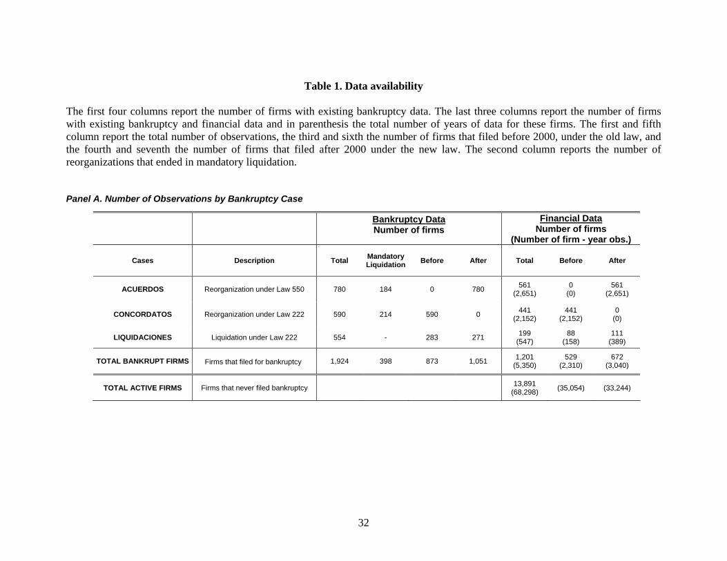
Table 1. Data availability The first four columns report the number of firms with existing bankruptcy data. The last three columns report the number of firms with existing bankruptcy and financial data and in parenthesis the total number of years of data for these firms. The first and fifth column report the total number of observations, the third and sixth the number of firms that filed before 2000, under the old law, and the fourth and seventh the number of firms that filed after 2000 under the new law. The second column reports the number of reorganizations that ended in mandatory liquidation.

Panel A. Number of Observations by Bankruptcy Case

Bankruptcy Data Number of firms

Financial Data Number of firms

(Number of firm - year obs.)

Cases Description Total Mandatory Liquidation Before After Total Before After

ACUERDOS Reorganization under Law 550 780 184 0 780 561 (2,651)

0 (0)

561 (2,651)

CONCORDATOS Reorganization under Law 222 590 214 590 0 441 (2,152)

441 (2,152)

0 (0)

LIQUIDACIONES Liquidation under Law 222 554 - 283 271 199 (547)

88 (158)

111 (389)

TOTAL BANKRUPT FIRMS Firms that filed for bankruptcy

1,924

398

873 1,051 1,201

(5,350) 529

(2,310) 672

(3,040)

TOTAL ACTIVE FIRMS

Firms that never filed bankruptcy 13,891

(68,298)

(35,054)

(33,244)

32

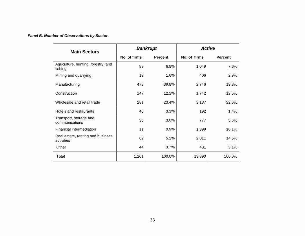
Panel B. Number of Observations by Sector

Bankrupt Active Main Sectors

No. of firms Percent No. of firms Percent

Agriculture, hunting, forestry, and fishing 83 6.9% 1,049 7.6%

Mining and quarrying 19 1.6% 406 2.9%

Manufacturing 478 39.8% 2,746 19.8%

Construction 147 12.2% 1,742 12.5%

Wholesale and retail trade 281 23.4% 3,137 22.6%

Hotels and restaurants 40 3.3% 192 1.4%

Transport, storage and communications 36 3.0% 777 5.6%

Financial intermediation 11 0.9% 1,399 10.1%

Real estate, renting and business activities 62 5.2% 2,011 14.5%

Other 44 3.7% 431 3.1%

Total 1,201 100.0% 13,890 100.0%

33

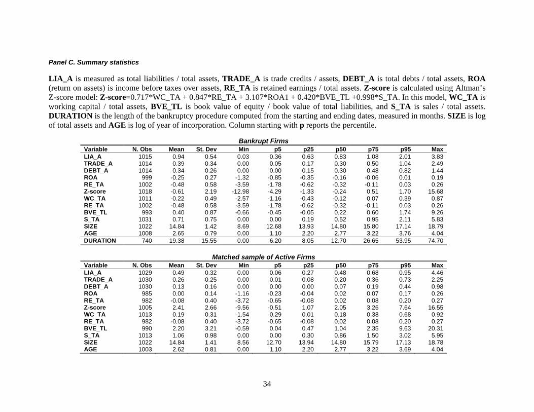
Panel C. Summary statistics LIA_A is measured as total liabilities / total assets, TRADE_A is trade credits / assets, DEBT_A is total debts / total assets, ROA (return on assets) is income before taxes over assets, RE_TA is retained earnings / total assets. Z-score is calculated using Altman’s Z-score model: Z-score=0.717*WC_TA + 0.847*RE_TA + 3.107*ROA1 + 0.420*BVE_TL +0.998*S_TA. In this model, WC_TA is working capital / total assets, BVE_TL is book value of equity / book value of total liabilities, and S_TA is sales / total assets. DURATION is the length of the bankruptcy procedure computed from the starting and ending dates, measured in months. SIZE is log of total assets and AGE is log of year of incorporation. Column starting with p reports the percentile.

Bankrupt Firms Variable N. Obs Mean St. Dev Min p5 p25 p50 p75 p95 Max LIA_A 1015 0.94 0.54 0.03 0.36 0.63 0.83 1.08 2.01 3.83 TRADE_A 1014 0.39 0.34 0.00 0.05 0.17 0.30 0.50 1.04 2.49 DEBT_A 1014 0.34 0.26 0.00 0.00 0.15 0.30 0.48 0.82 1.44 ROA 999 -0.25 0.27 -1.32 -0.85 -0.35 -0.16 -0.06 0.01 0.19 RE_TA 1002 -0.48 0.58 -3.59 -1.78 -0.62 -0.32 -0.11 0.03 0.26 Z-score 1018 -0.61 2.19 -12.98 -4.29 -1.33 -0.24 0.51 1.70 15.68 WC_TA 1011 -0.22 0.49 -2.57 -1.16 -0.43 -0.12 0.07 0.39 0.87 RE_TA 1002 -0.48 0.58 -3.59 -1.78 -0.62 -0.32 -0.11 0.03 0.26 BVE_TL 993 0.40 0.87 -0.66 -0.45 -0.05 0.22 0.60 1.74 9.26 S_TA 1031 0.71 0.75 0.00 0.00 0.19 0.52 0.95 2.11 5.83 SIZE 1022 14.84 1.42 8.69 12.68 13.93 14.80 15.80 17.14 18.79 AGE 1008 2.65 0.79 0.00 1.10 2.20 2.77 3.22 3.76 4.04 DURATION 740 19.38 15.55 0.00 6.20 8.05 12.70 26.65 53.95 74.70

Matched sample of Active Firms Variable N. Obs Mean St. Dev Min p5 p25 p50 p75 p95 Max LIA_A 1029 0.49 0.32 0.00 0.06 0.27 0.48 0.68 0.95 4.46 TRADE_A 1030 0.26 0.25 0.00 0.01 0.08 0.20 0.36 0.73 2.25 DEBT_A 1030 0.13 0.16 0.00 0.00 0.00 0.07 0.19 0.44 0.98 ROA 985 0.00 0.14 -1.16 -0.23 -0.04 0.02 0.07 0.17 0.26 RE_TA 982 -0.08 0.40 -3.72 -0.65 -0.08 0.02 0.08 0.20 0.27 Z-score 1005 2.41 2.66 -9.56 -0.51 1.07 2.05 3.26 7.64 16.55 WC_TA 1013 0.19 0.31 -1.54 -0.29 0.01 0.18 0.38 0.68 0.92 RE_TA 982 -0.08 0.40 -3.72 -0.65 -0.08 0.02 0.08 0.20 0.27 BVE_TL 990 2.20 3.21 -0.59 0.04 0.47 1.04 2.35 9.63 20.31 S_TA 1013 1.06 0.98 0.00 0.00 0.30 0.86 1.50 3.02 5.95 SIZE 1022 14.84 1.41 8.56 12.70 13.94 14.80 15.79 17.13 18.78 AGE 1003 2.62 0.81 0.00 1.10 2.20 2.77 3.22 3.69 4.04

34

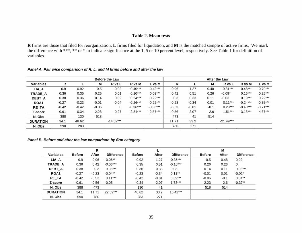
Table 2. Mean tests R firms are those that filed for reorganization, L firms filed for liquidation, and M is the matched sample of active firms. We mark the difference with ***, ** or * to indicate significance at the 1, 5 or 10 percent level, respectively. See Table 1 for definition of variables. Panel A. Pair wise comparison of R, L, and M firms before and after the law

Before the Law After the Law Variables R L M R vs L R vs M L vs M R L M R vs L R vs M L vs M

LIA_A 0.9 0.92 0.5 -0.02 0.40*** 0.42*** 0.96 1.27 0.48 -0.31*** 0.48*** 0.79*** TRADE_A 0.36 0.35 0.26 0.01 0.10*** 0.09*** 0.42 0.51 0.26 -0.09* 0.16*** 0.25*** DEBT_A 0.38 0.36 0.14 0.02 0.24*** 0.22*** 0.3 0.33 0.11 -0.03 0.19*** 0.22***

ROA1 -0.27 -0.23 -0.01 -0.04 -0.26*** -0.22*** -0.23 -0.34 0.01 0.11*** -0.24*** -0.35*** RE_TA -0.42 -0.42 -0.06 0 -0.36*** -0.36*** -0.53 -0.81 -0.1 0.28*** -0.43*** -0.71*** Z-score -0.61 -0.34 2.23 -0.27 -2.84*** -2.57*** -0.56 -2.07 2.6 1.51*** -3.16*** -4.67*** N. Obs 388 130 518 473 41 514

DURATION 34.1 48.62 -14.52*** 11.71 33.2 -21.49*** N. Obs 590 283 780 271

Panel B. Before and after the law comparison by firm category

R L M Variables Before After Difference Before After Difference Before After Difference

LIA_A 0.9 0.96 -0.06** 0.92 1.27 -0.35*** 0.5 0.48 0.02 TRADE_A 0.36 0.42 -0.06*** 0.35 0.51 -0.16*** 0.26 0.26 0 DEBT_A 0.38 0.3 0.08*** 0.36 0.33 0.03 0.14 0.11 0.03***

ROA1 -0.27 -0.23 -0.04** -0.23 -0.34 0.11** -0.01 0.01 -0.02* RE_TA -0.42 -0.53 0.11*** -0.42 -0.81 0.39*** -0.06 -0.1 0.04** Z-score -0.61 -0.56 -0.05 -0.34 -2.07 1.73*** 2.23 2.6 -0.37** N. Obs 388 473 130 41 518 514

DURATION 34.1 11.71 22.39*** 48.62 33.2 15.42*** N. Obs 590 780 283 271

35

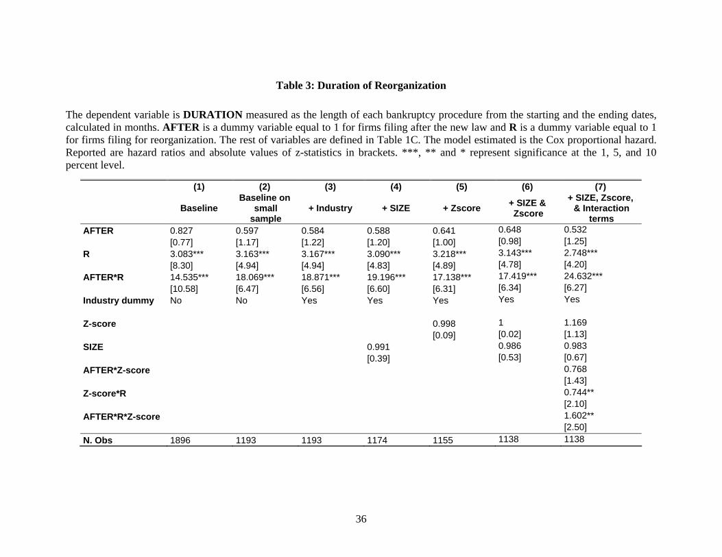
Table 3: Duration of Reorganization

The dependent variable is DURATION measured as the length of each bankruptcy procedure from the starting and the ending dates, calculated in months. AFTER is a dummy variable equal to 1 for firms filing after the new law and R is a dummy variable equal to 1 for firms filing for reorganization. The rest of variables are defined in Table 1C. The model estimated is the Cox proportional hazard. Reported are hazard ratios and absolute values of z-statistics in brackets. ***, ** and * represent significance at the 1, 5, and 10 percent level.

(1) (2) (3) (4) (5) (6) (7)

Baseline Baseline on

small sample

+ Industry + SIZE + Zscore + SIZE & Zscore

+ SIZE, Zscore, & Interaction

terms AFTER 0.827 0.597 0.584 0.588 0.641 0.648 0.532 [0.77] [1.17] [1.22] [1.20] [1.00] [0.98] [1.25] R 3.083*** 3.163*** 3.167*** 3.090*** 3.218*** 3.143*** 2.748*** [8.30] [4.94] [4.94] [4.83] [4.89] [4.78] [4.20] AFTER*R 14.535*** 18.069*** 18.871*** 19.196*** 17.138*** 17.419*** 24.632*** [10.58] [6.47] [6.56] [6.60] [6.31] [6.34] [6.27] Industry dummy No No Yes Yes Yes Yes Yes Z-score 0.998 1 1.169 [0.09]

[0.39]

[0.02] [1.13] SIZE 0.991 0.986 0.983 [0.53] [0.67] AFTER*Z-score 0.768 [1.43] Z-score*R 0.744** [2.10] AFTER*R*Z-score 1.602** [2.50] N. Obs 1896 1193 1193 1138 1138 1174 1155

36

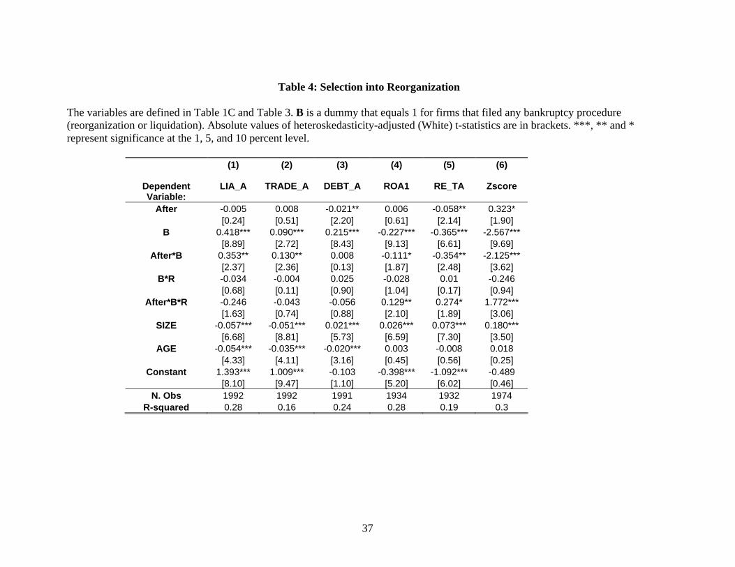
Table 4: Selection into Reorganization The variables are defined in Table 1C and Table 3. B is a dummy that equals 1 for firms that filed any bankruptcy procedure (reorganization or liquidation). Absolute values of heteroskedasticity-adjusted (White) t-statistics are in brackets. ***, ** and * represent significance at the 1, 5, and 10 percent level.

(1) (2) (3) (4) (5) (6)

Dependent Variable:

LIA_A TRADE_A DEBT_A ROA1 RE_TA Zscore

After -0.005 0.008 -0.021** 0.006 -0.058** 0.323* [0.24] [0.51] [2.20] [0.61] [2.14] [1.90]

B 0.418*** 0.090*** 0.215*** -0.227*** -0.365*** -2.567*** [8.89] [2.72] [8.43] [9.13] [6.61] [9.69]

After*B 0.353** 0.130** 0.008 -0.111* -0.354** -2.125*** [2.37] [2.36] [0.13] [1.87] [2.48] [3.62]

B*R -0.034 -0.004 0.025 -0.028 0.01 -0.246 [0.68] [0.11] [0.90] [1.04] [0.17] [0.94]

After*B*R -0.246 -0.043 -0.056 0.129** 0.274* 1.772*** [1.63] [0.74] [0.88] [2.10] [1.89] [3.06]

SIZE -0.057*** -0.051*** 0.021*** 0.026*** 0.073*** 0.180*** [6.68] [8.81] [5.73] [6.59] [7.30] [3.50]

AGE -0.054*** -0.035*** -0.020*** 0.003 -0.008 0.018 [4.33] [4.11] [3.16] [0.45] [0.56] [0.25]

Constant 1.393*** 1.009*** -0.103 -0.398*** -1.092*** -0.489 [8.10] [9.47] [1.10] [5.20] [6.02] [0.46]

N. Obs 1992 1992 1991 1934 1932 1974 R-squared 0.28 0.16 0.24 0.28 0.19 0.3

37

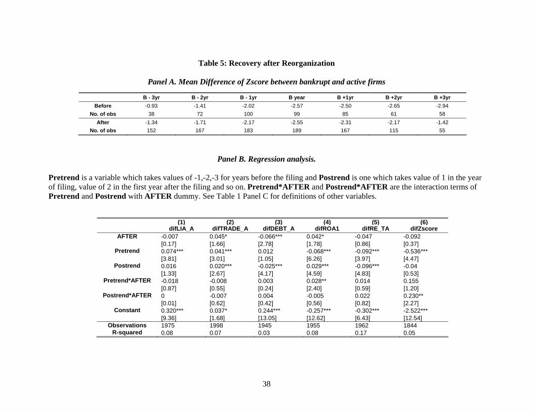
Table 5: Recovery after Reorganization

Panel A. Mean Difference of Zscore between bankrupt and active firms

B - 3yr B - 2yr B - 1yr B year B +1yr B +2yr B +3yr Before -0.93 -1.41 -2.02 -2.57 -2.50 -2.65 -2.94

No. of obs 38 72 100 99 85 61 58 After -1.34 -1.71 -2.17 -2.55 -2.31 -2.17 -1.42

No. of obs 152 167 183 189 167 115 55

Panel B. Regression analysis.

Pretrend is a variable which takes values of -1,-2,-3 for years before the filing and Postrend is one which takes value of 1 in the year of filing, value of 2 in the first year after the filing and so on. Pretrend*AFTER and Postrend*AFTER are the interaction terms of Pretrend and Postrend with AFTER dummy. See Table 1 Panel C for definitions of other variables.

(1) (2) (3) (4) (5) (6) difLIA_A difTRADE_A difDEBT_A difROA1 difRE_TA difZscore

AFTER -0.007 0.045* -0.066*** 0.042* -0.047 -0.092 [0.17] [1.66] [2.78] [1.78] [0.86] [0.37]

Pretrend 0.074*** 0.041*** 0.012 -0.068*** -0.092*** -0.536*** [3.81] [3.01] [1.05] [6.26] [3.97] [4.47]

Postrend 0.016 0.020*** -0.025*** 0.029*** -0.096*** -0.04 [1.33] [2.67] [4.17] [4.59] [4.83] [0.53]

Pretrend*AFTER -0.018 -0.008 0.003 0.028** 0.014 0.155 [0.87] [0.55] [0.24] [2.40] [0.59] [1.20]

Postrend*AFTER 0 -0.007 0.004 -0.005 0.022 0.230** [0.01] [0.62] [0.42] [0.56] [0.82] [2.27]

Constant 0.320*** 0.037* 0.244*** -0.257*** -0.302*** -2.522*** [9.36] [1.68] [13.05] [12.62] [6.43] [12.54]

Observations 1975 1998 1945 1955 1962 1844 R-squared 0.08 0.07 0.03 0.08 0.17 0.05

38

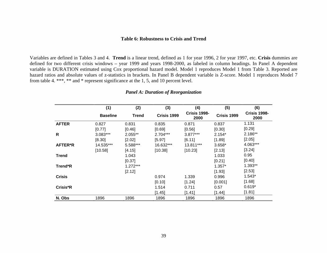
Table 6: Robustness to Crisis and Trend

Variables are defined in Tables 3 and 4. Trend is a linear trend, defined as 1 for year 1996, 2 for year 1997, etc. Crisis dummies are defined for two different crisis windows – year 1999 and years 1998-2000, as labeled in column headings. In Panel A dependent variable is DURATION estimated using Cox proportional hazard model. Model 1 reproduces Model 1 from Table 3. Reported are hazard ratios and absolute values of z-statistics in brackets. In Panel B dependent variable is Z-score. Model 1 reproduces Model 7 from table 4. ***, ** and * represent significance at the 1, 5, and 10 percent level.

Panel A: Duration of Reorganization

(1) (2) (3) (4) (5) (6)

Baseline Trend Crisis 1999 Crisis 1998-2000 Crisis 1999 Crisis 1998-

2000 AFTER 0.827 0.831 0.835 0.871 0.837 1.131 [0.77] [0.46] [0.69] [0.56] [0.30] [0.29] R 3.083*** 2.055** 2.704*** 3.877*** 2.154* 2.186** [8.30] [2.02] [5.97] [6.11] [1.89] [2.05] AFTER*R 14.535*** 5.588*** 16.632*** 13.811*** 3.658* 4.063*** [10.58] [4.15] [10.38] [10.23] [2.13] [3.24] Trend 1.043 1.033 0.95 [0.37] [0.21] [0.40] Trend*R 1.272*** 1.357* 1.393** [2.12] [1.93] [2.53] Crisis 0.974 1.339 0.996 1.543* [0.10] [1.24] [0.001] [1.68] Crisis*R 1.514 0.711 0.57 0.619* [1.45] [1.41] [1.44] [1.81] N. Obs 1896 1896 1896 1896 1896 1896

39

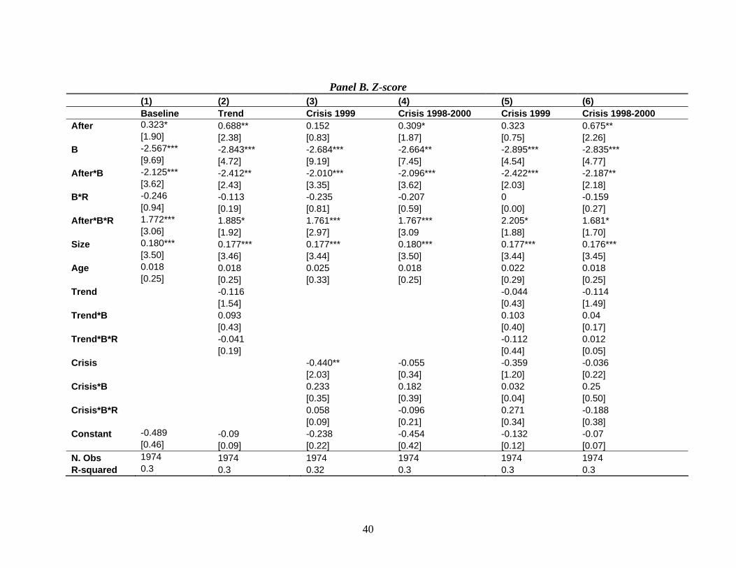
Panel B. Z-score (1) (2) (3) (4) (5) (6) Baseline Trend Crisis 1999 Crisis 1998-2000 Crisis 1999 Crisis 1998-2000 After 0.323* 0.688** 0.152 0.309* 0.323 0.675** [1.90] [2.38] [0.83] [1.87] [0.75] [2.26] B -2.567*** -2.843*** -2.684*** -2.664** -2.895*** -2.835*** [9.69] [4.72] [9.19] [7.45] [4.54] [4.77] After*B -2.125*** -2.412** -2.010*** -2.096*** -2.422*** -2.187** [3.62] [2.43] [3.35] [3.62] [2.03] [2.18] B*R -0.246 -0.113 -0.235 -0.207 0 -0.159 [0.94] [0.19] [0.81] [0.59] [0.00] [0.27] After*B*R 1.772*** 1.885* 1.761*** 1.767*** 2.205* 1.681* [3.06] [1.92] [2.97] [3.09 [1.88] [1.70] Size 0.180*** 0.177*** 0.177*** 0.180*** 0.177*** 0.176*** [3.50] [3.46] [3.44] [3.50] [3.44] [3.45] Age 0.018 0.018 0.025 0.018 0.022 0.018 [0.25] [0.25] [0.33] [0.25] [0.29] [0.25] Trend -0.116 -0.044 -0.114 [1.54] [0.43] [1.49] Trend*B 0.093 0.103 0.04 [0.43] [0.40] [0.17] Trend*B*R -0.041 -0.112 0.012 [0.19] [0.44] [0.05] Crisis -0.440** -0.055 -0.359 -0.036 [2.03] [0.34] [1.20] [0.22] Crisis*B 0.233 0.182 0.032 0.25 [0.35] [0.39] [0.04] [0.50] Crisis*B*R 0.058 -0.096 0.271 -0.188 [0.09] [0.21] [0.34] [0.38] Constant -0.489 -0.09 -0.238 -0.454 -0.132 -0.07 [0.46] [0.09] [0.22] [0.42] [0.12] [0.07] N. Obs 1974 1974 1974 1974 1974 1974 R-squared 0.3 0.3 0.32 0.3 0.3 0.3

40

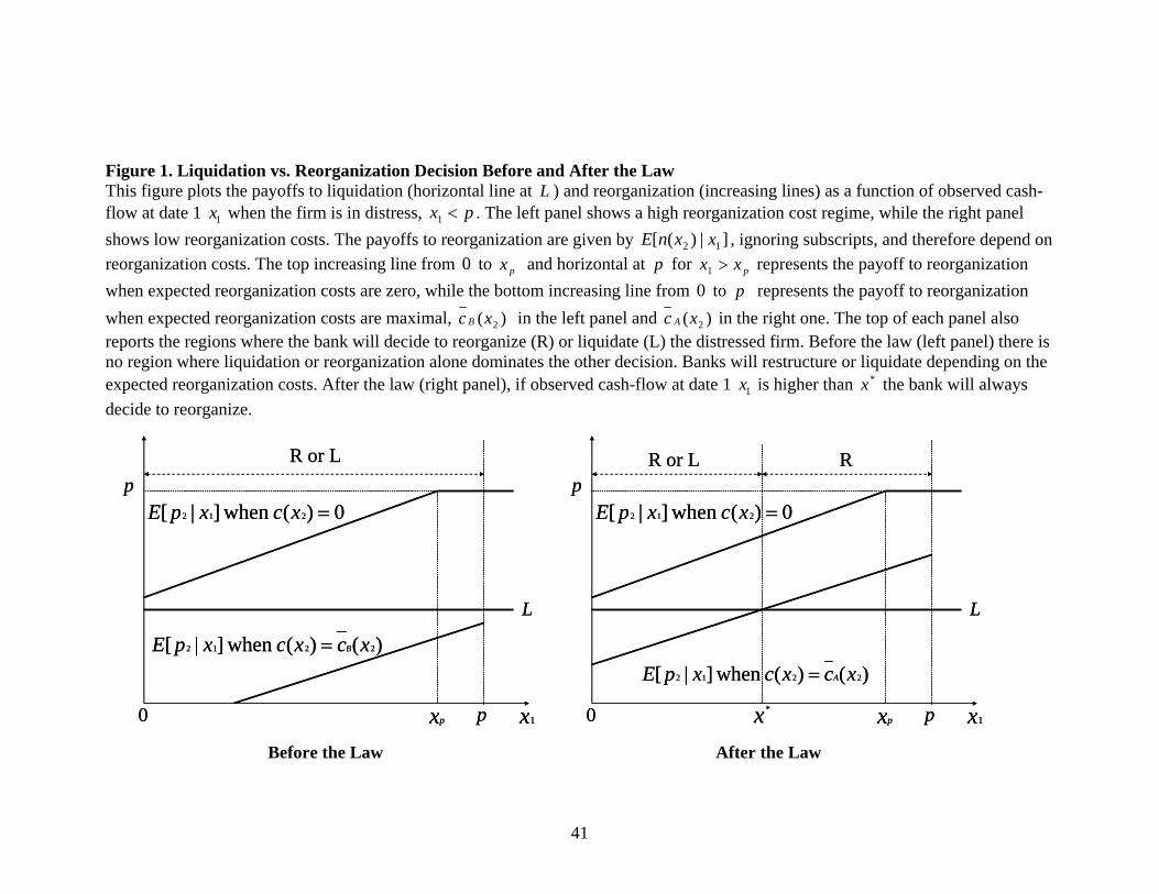
Figure 1. Liquidation vs. Reorganization Decision Before and After the Law This figure plots the payoffs to liquidation (horizontal line at L ) and reorganization (increasing lines) as a function of observed cash-flow at date 1 1x when the firm is in distress, px <1 . The left panel shows a high reorganization cost regime, while the right panel shows low reorganization costs. The payoffs to reorganization are given by , ignoring subscripts, and therefore depend on reorganization costs. The top increasing line from 0 to and horizontal at for represents the payoff to reorganization when expected reorganization costs are zero, while the bottom increasing line from to represents the payoff to reorganization when expected reorganization costs are maximal,

]|)([ 12 xxnEpx p pxx >1

0 p)( 2xc B in the left panel and )( 2xc A in the right one. The top of each panel also

reports the regions where the bank will decide to reorganize (R) or liquidate (L) the distressed firm. Before the law (left panel) there is no region where liquidation or reorganization alone dominates the other decision. Banks will restructure or liquidate depending on the expected reorganization costs. After the law (right panel), if observed cash-flow at date 1 1x is higher than *x the bank will always decide to reorganize.

1x

L

0)( when ]|[ 212 =xcxpE

Before the Law After the Law

p

p0

)()( when ]|[ 2212 xcxcxpE B=

R or L

px 1x

L

0)( when ]|[ 212 =xcxpEp

p0 *x

)()( when ]|[ 2212 xcxcxpE A=

R or L R

px 1x

L

0)( when ]|[ 212 =xcxpEp

p0 *x

)()( when ]|[ 2212 xcxcxpE A=

R or L R

px1x

L

0)( when ]|[ 212 =xcxpEp

)()( when ]|[ 2212 xcxcxpE B=

R or L

p0 px

41

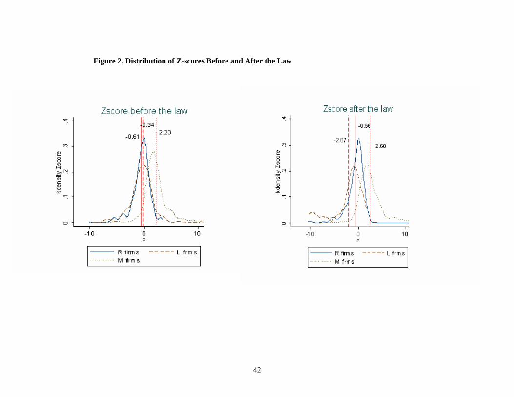
Figure 2. Distribution of Z-scores Before and After the Law

42

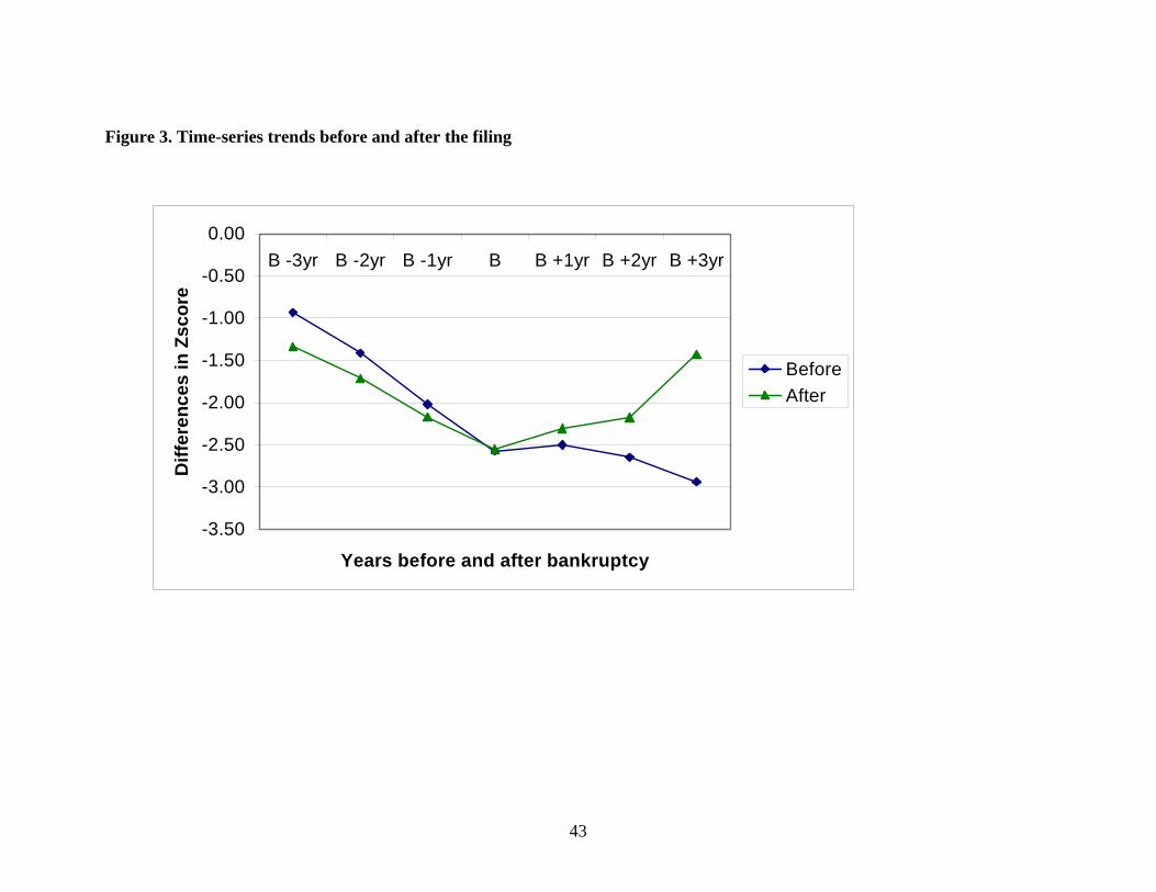
Figure 3. Time-series trends before and after the filing

-3.50

-3.00

-2.50

-2.00

-1.50

-1.00

-0.50

0.00B -3yr B -2yr B -1yr B B +1yr B +2yr B +3yr

Years before and after bankruptcy

Diff

eren

ces

in Z

scor

e

BeforeAfter

43