cs.uccs.educs.uccs.edu/~gsc/pub/master/phuynh/doc/phuynhThesisV1.docx · Web viewThe SkyPilot’s mesh network solution combines standard-based Wi-Fi access with a high performance

SIMULATION AND ANALYSIS OF WIRELESS MESH NETWORK

IN SMART GRID – ADVANCED METERRING INFRASTRUCTURE

by

PHILIP HUU HUYNH

B.A., The University of Economic, Vietnam, 1996.

A thesis submitted to the Faculty of Graduate School of the

University of Colorado at Colorado Springs

in partial fulfillment of the

requirements for the degree of

Master of Science

Department of Computer Science

2011

ii

Thesis for the Master of Science degree by

Philip Huu Huynh

has been approved for the


by

_______________________________________________________

Advisor: Dr. C. Edward Chow

_______________________________________________________

Dr. Jugal K. Kalita

_______________________________________________________

Dr. Rory Lewis

_____________________

Date

iii

Simulation and Analysis of Wireless Mesh Network in

Smart Grid – Advanced Meterring Infrastructure

by

Philip Huu Huynh

Master of Science, Computer Science

Thesis directed by Associate Dean Professor C. Edward Chow


Abstract

In this thesis the use of Wireless Mesh Network (WMN) technologies as the Advanced

Metering Infrastructure (AMI) for the collecting of meter data in real-time was proposed

and analyzed. A Google Maps mashup was developed to display the locations of the

meters and light poles, which can be selected for mounting the WiMAX or Wi-Fi

network devices. A NS-3 simulator was developed to simulate the network traffic of

meter data collection over the WMN and to allow us evaluating different topologies and

to see if their capacities are adequate to report all meter values to the data center within

one second. A JavaScript program was developed to analyze the meter density within

different service areas of Colorado Springs Utilities. The information can be used for

antennae placement planning.

We proposed a hybrid WiMAX and Wi-Fi mesh network to address the cost and

efficiency issues. In local service area, we can use lower cost Wi-Fi mesh network to

iv

connect smart meters to the WiMAX Base Stations. From those WiMAX Base Stations,

we utilize the long distance links provided by WiMAX point-to-point connection mode to

collect meters from a local service areas to a handful of take out points. From take-out

points, high speed optical fiber connections are to be used transport the meter data to the

data center. We evaluate the design trade offs of these WMN choices through the NS-3

simulations. The simulation results show that with this type of WMN (6 WiMAX Base

Stations and 540 Wi-Fi Access Points), it is feasible to collect meter data from 150,000

smart meters within one second.

The Smart Grid Wireless Infrastructure Planning (SG-WIP) Google Maps mashup tool

can be integrated with the simulator and allow the planner to interactively adjust the

planning of wireless network devices such as WiMAX Base Stations, or Wi-Fi Access

Points on the light poles in certain service areas.

v

Acknowledgments

(will fill the content to thank Dr. Chow, Faculty, CSU)

vi

Table of Contents

(will fill the table of contents)

vii

List of Tables

(will fill the list of tables)

viii

List of Figures

(will fill list of figures)

Chapter 1IntroductionRecently many utilities started to deploy smart grids for collecting meter data [1, 5].

The main reasons are to reduce the cost by not sending people to read the meter data and

by avoiding generating excess power through correct prediction of the load profile using

the aggregated meter values. To correctly predict the load profile and perform load

forecasting, utilities need to collect meter data in real time.

Utilities have hundreds of thousands of meters installed in their service areas, and want to

network these meters for metering collection. The wireless communication technologies

have been popularly deployed in the local areas and the metropolitan areas because of

their conveniences in the cost, network installation and maintenance. Taking advantages

of the wireless technologies, utilities can network their meters and the data center for data

communication. However, if the underlined wireless technologies do not provide enough

bandwidth, then the meter data cannot be delivered to the data center in time. The

WiMAX technology allows us networking the meters and the data center with the

broadband data transmission at long distance and higher bandwidth [8, 20]. Therefore,

the wireless networking solution for real-time metering collection is feasible. The

important question is to design of the wireless infrastructure and their topology so that it

can be scaled up and meet the cost and real-time performance requirements, given huge

wireless meters to be served in large areas. For example, The Wi-Fi mesh technology

2

can be employed as part of a hybrid wireless infrastructure with WiMAX and Wi-Fi to

allow the deployment at the reasonable low cost [7, 14].

The wireless technologies such as WiMAX, and Wi-Fi are high performance, scalable,

and secured [14]. Taking the advantages of these network technologies, utilities can

deploy the smart grid wireless communications infrastructure for the real-time metering

collection. The real-time meter data can save the operation costs and reduce the

electricity market price.

1.1 Thesis Statement

In this thesis we plan to address the following important question: Is the wireless mesh

network infrastructure applicable for the real-time meter data collection? It is a

challenge facing the smart grid wireless infrastructure planners. We intend to conduct a

simulation analysis of the wireless communication infrastructure for the smart grid to

answer this question.

1.2 Goals

In this thesis, we propose to research and develop a wireless communication

infrastructure solution using the wireless mesh network technologies for the smart grid.

Tools and techniques will be developed for the planning and designing the wireless

infrastructure. The performance and scalability properties of the proposed wireless

infrastructure are evaluated. We focus on these network properties because they are the

important factors that affect the performance of the real-time meter data collection.

3

1.3 Contributions

This thesis will contribute to the smart grid research by investigating the wireless mesh

network that is employed as a communication infrastructure solution for the real-time

metering collection. The wireless infrastructure planning tools in this thesis will benefit

not only the researchers but also the utilities. The network infrastructure planners and

researchers can use the planning tools to conduct surveys about wireless network

topologies. Moreover, the infrastructure planners and designers can use the tools to refine

their network designs.

Another contribution of this thesis is to provide a communication network solution that is

low cost, and secured. It allows the utilities to have an alternative option for their AMI

wireless infrastructure. The proposed wireless infrastructure with the wireless mesh

technologies are cheap, far-reaching, and scalable.

Chapter 2Background and Related Works

2.1 Introduction to Smart Grid / Advanced Metering

Infrastructure

Growing the need for the Smart Grid (SG)

A smart grid [1, 2, 3] delivers electricity from suppliers to consumers using two-way

digital communication technology. Smart grid allows controlling appliances at

consumer’s homes to save energy, and reduce cost. The operation status of the smart

grids can be monitored in real time, so the smart grids are more reliable. Many

governments are promoting such a modernized electricity network as a way of addressing

energy independence, global warming and emergency resilience issues.

5

Figure 2. 1 Smart grid overview (source: U.S. Department of Energy)

Figure 2.1 shows an overview of the smart grid. Utilities can archive energy efficiency

and maintain the competitive of services by taking advantages of the smart grid and its

market benefits. The smart grid solutions that utilize the information technology for data

collection, monitoring and control, data analysis and information communication

infrastructure, will cost-effectively protect revenues today, while laying the foundations

for future services.

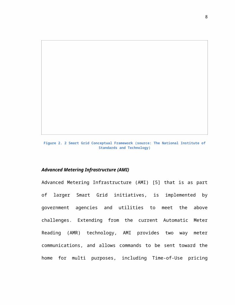
Figure 2.2 shows the conceptual framework of smart grid. The components includes

Service Provider, Operations, Markets, Bulk Generation, Transmission, Distribution, and

Customer.

6

Figure 2. 2 Smart Grid Conceptual Framework (source: The National Institute of Standards and Technology)

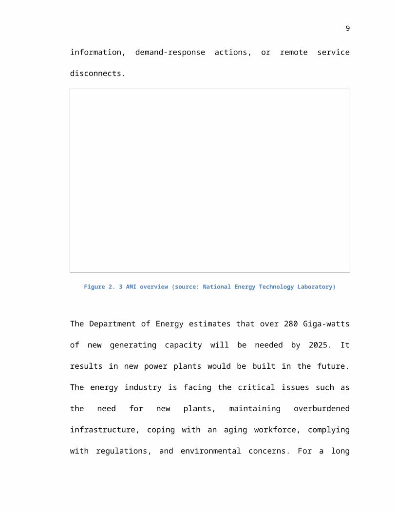
Advanced Metering Infrastructure (AMI)

Advanced Metering Infrastructure (AMI) [5] that is as part of larger Smart Grid

initiatives, is implemented by government agencies and utilities to meet the above

challenges. Extending from the current Automatic Meter Reading (AMR) technology,

AMI provides two way meter communications, and allows commands to be sent toward

the home for multi purposes, including Time-of-Use pricing information, demand-

response actions, or remote service disconnects.

7

Figure 2. 3 AMI overview (source: National Energy Technology Laboratory)

The Department of Energy estimates that over 280 Giga-watts of new generating capacity

will be needed by 2025. It results in new power plants would be built in the future. The

energy industry is facing the critical issues such as the need for new plants, maintaining

overburdened infrastructure, coping with an aging workforce, complying with

regulations, and environmental concerns. For a long time, the energy industry has

rightfully focused on the supply side of this challenge. But now, the demand side of the

equation can be significantly impacted by the existing of the wireless mesh networking

[13].

8

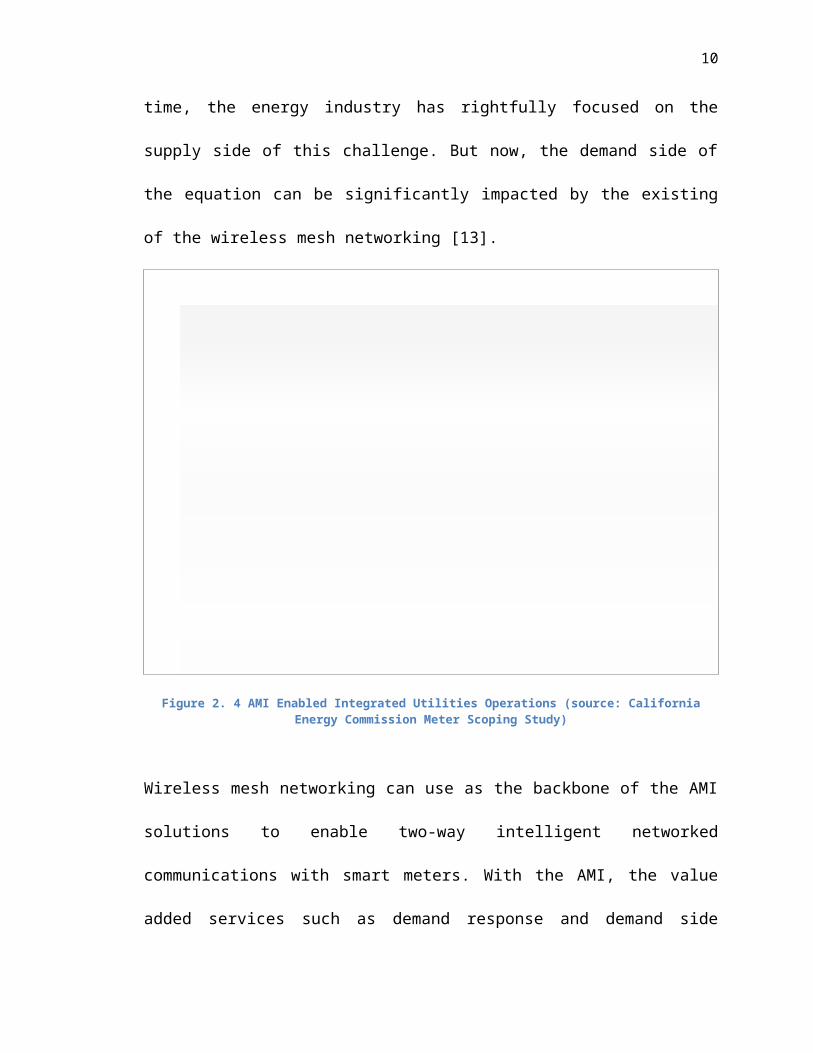
Figure 2. 4 AMI Enabled Integrated Utilities Operations (source: California Energy Commission Meter Scoping Study)

Wireless mesh networking can use as the backbone of the AMI solutions to enable two-

way intelligent networked communications with smart meters. With the AMI, the value

added services such as demand response and demand side management would be

enabled, besides meter reading. AMI solutions allows interoperable networks and

systems across the entire power structure aid in the management and control of energy

consumption, improve operations management, conserve the environment, and adhere to

evolving regulations [5].

2.2 Introduction to Wireless Mesh Network (WMN)

9

What is WMN?

A WMN [7, 10, 11] is a communications network made up of radio nodes organized in a

mesh topology. Wireless mesh networks often consist of mesh clients, mesh routers and

gateways. The mesh clients are often laptops, cell phones and other wireless devices

while the mesh routers forward traffic to and from the gateways which may but need not

connect to the Internet. A mesh network is reliable and offers redundancy. When one

node can no longer operate, the rest of the nodes can still communicate with each other,

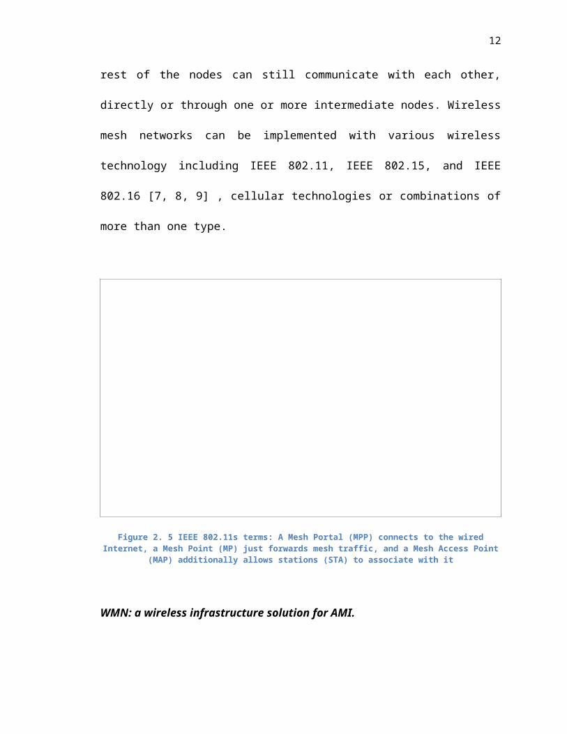
directly or through one or more intermediate nodes. Wireless mesh networks can be

implemented with various wireless technology including IEEE 802.11, IEEE 802.15, and

IEEE 802.16 [7, 8, 9] , cellular technologies or combinations of more than one type.

Figure 2. 5 IEEE 802.11s terms: A Mesh Portal (MPP) connects to the wired Internet, a Mesh Point (MP) just forwards mesh traffic, and a Mesh Access Point (MAP) additionally allows stations (STA) to associate with it

WMN: a wireless infrastructure solution for AMI.

10

When the WMN technology is applied in AMI solutions, it can bring new components to

the electrical grids, such as self-managing and self-healing mesh networking, intelligent

meters, and bridging to Home Area Networks (HAN) [5] for connectivity with energy

consuming appliances. The real time communication between the smart meters and the

utility’s data center provides detailed usage data while also receives and display Time-of-

Use (TOU) pricing information, and offers other on-demand abilities such as remote

connect or disconnect, unrestricted monitoring and control, etc. Customers are able to

access the usage data for tailoring consumption and minimizing energy expenses while

helping balance overall network demand.

When WMNs are used in the AMI, they can provide the following features [13, 18]:

Low cost of management and maintenance - WMNs are self-organizing and

require no manual address/route/channel assignments. It is simple to manage

thousands or millions of devices resulting in the lowest total cost of ownership.

Increased reliability – The WMN routing mechanisms provide the redundant paths

between the sender and receiver of the wireless connection. Communication

reliability is significantly increased because of the eliminations of single point

failures and potential bottleneck links. Network robustness against potential

problems, e.g., node failures and path failures due to RF interferences or obstacles,

can also be ensured by the existence of multiple possible alternative routes.

Scalability, flexibility and lower costs - WMNs are self-organizing and allow true

scalability. Nodes and Gateways are easily added at a very low cost with:

o No limitation on number of hops

o No network address configuration

11

o No managed hierarchical architecture

o No hard limitation on number of Nodes per Gateway

Robust security – WMNs have the security standards that allows all

communications in AMI are protected by mutual device authentication and derived

per-session keys using high bit rate AES encryption. This hardened security

approach allows for authentication as well as confidentiality and integrity

protection in each communication exchange between every pair of network

devices – Smart meters, Relays, or Wireless Gateways.

2.3 Related Works

2.3.1 Colorado Springs Utility AMI Network Infrastructure

A brief introduction

The Colorado Springs Utility AMI wireless network infrastructure used the Point-to-

Multi Point topology where 902-928MHz concentrators are used to collect meter data in

a neighbor area mounting on the light pole, eight take-out points are used to poll and

collect meter data from hundreds of concentrators. Telecommunication links and fiber

connections are used to connect take-out points to the data center. The current meter data

reading interval is five minutes for electric, fifteen minutes for gas and water meters [6].

2.3.2 SkyPilot’s Synchronous Mesh Network Solution


12

MetroFi has deployed a mesh network in the Silicon Valley – California [ref]. The

installed wireless mesh metropolitan area network can provide the Internet access service

to the resident user in a geographical area that covers about 250,000 households. The

SkyPilot’s Synchronous Mesh Network solution was employed to build this mesh

network. The SkyPilot’s mesh network solution combines standard-based Wi-Fi access

with a high performance wireless mesh backhaul network using SkyGate nodes to

interface with the Internet, SkyExtender DualBand nodes that integrate Wi-Fi access and

mesh backhaul [15].

Figure 2. 7 SkyPilot Mesh Network Architecture (source: SkyPilot)

The mesh network MetroFi is a success deployment of the WMN onto the large

geographical area. However, in the AMI meter data collection application, there is a

different in the network traffic pattern compared to the regular Web applications. The

Web applications usually need the connection with low bandwidth uplink, and high

Figure 2. 6 A SkyExtender was installed on the street light pole (source: SkyPilot)

13

bandwidth downlink. In contrast, the AMI meter data reporting process requires the high

bandwidth uplink connections to send the data from smart meters to data center.

We can make an assumption that we intend to use the MetroFi network for the AMI

communication infrastructure solution. Then, there is a research opportunity about the

MetroFi or WMN performance – Whether the WMN is suitable for the AMI network

infrastructure, especially for the real-time meter data reporting application?

2.3.3 EkaNet™ Smart Network - Wireless mesh network

solution for the Smart grid/AMI


The wireless mesh infrastructure EkaNet [16] includes the smart meter nodes, ranger

extension nodes, and gateway nodes. The smart meter nodes are networking together to

form the wireless mesh network. It means that, the communication between a smart meter

node and the gateway will replay on a number of other smart meters. The range extension

nodes are used to help connect the out of coverage nodes. The gateway nodes provide the

interface to the Internet network.

14

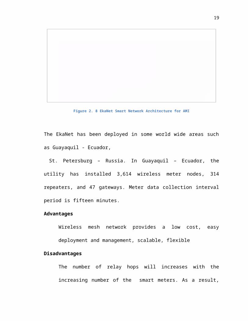
Figure 2. 8 EkaNet Smart Network Architecture for AMI

The EkaNet has been deployed in some world wide areas such as Guayaquil - Ecuador,

St. Petersburg – Russia. In Guayaquil – Ecuador, the utility has installed 3,614 wireless

meter nodes, 314 repeaters, and 47 gateways. Meter data collection interval period is

fifteen minutes.

Advantages

Wireless mesh network provides a low cost, easy deployment and management,

scalable, flexible

Disadvantages

The number of relay hops will increases with the increasing number of the smart

meters. As a result, the network performance will go down fast, especially in the

service place where the smart meter density is high, i.e. hundreds of smart meters

in the area 100 meters by 100 meters. In the high resident density area, the mesh

topology will not be a good choice for the network performance goal. Instead, the

point-to-multipoint topology such as Wi-Fi infrastructure mode would provide a

better network performance.

15

2.3.4 “Coverage and Capacity of A Wireless Mesh

Network” – A research conducted by –H. Huang, L. -C.

Wang, C. -J. Chang


The authors proposed a multi-channel ring-based wireless mesh network and develop an

analytical framework to evaluate the capacity and coverage of such a network [32]. They

suggested a distance-based rate adaption scheme and established a PHY/MAC cross-layer

performance model based on the CSMA MAC protocol with RTS/CTS. Based on the

derived throughput model, they apply the mixed-integer nonlinear programming

optimization approach to maximize the capacity (throughput) and service coverage of a

mesh cell, in which the number of rings in a mesh cell and the radius for each ring are

determined.

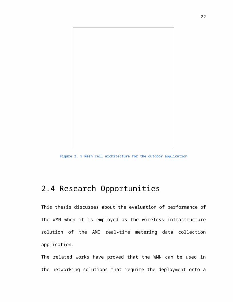
The Figure 2.9 shows the proposed architecture of an outdoor WMN [32]. The authors

define a mesh cell is a cell in which each user forwards or relays traffic for others to the

central gateway. In each mesh cell, only the gateway connects directly to the Internet.

16

Figure 2. 9 Mesh cell architecture for the outdoor application

2.4 Research Opportunities

This thesis discusses about the evaluation of performance of the WMN when it is

employed as the wireless infrastructure solution of the AMI real-time metering data

collection application.

The related works have proved that the WMN can be used in the networking solutions

that require the deployment onto a large geographical area, such as the AMR/AMI

metering data collection application. However, the WMN infrastructure needs a high

bandwidth for transmitting the meter data from the smart meters to the data center in real-

17

time. The conducted researches have shown that the WMN network bandwidth is

affected by the hop number. The more hop number is the WMN routing path, the less

performance is the WMN [18, 19, 21].

2.5 Summary

In general, the wireless mesh network infrastructure can provides a cheap solution,

compared to the wire network, connecting the smart meters to the utility data center.

However, to answer the challenge question, whether the wireless mesh infrastructure is

suitable for the real-time meter data reporting process, this thesis will go into more detail

in the analysis of the performance property of the wireless network infrastructure

solution. We will develop new tools and techniques to assist the planning and design

phase. We will also use the network simulation method to evaluate the network

performance.

Chapter 3Problem and Solution

3.1 Problem Statement

The WMN contributes many advantages to the AMI Communication Network solution.

However, there are challenge questions in planning, designing and deployment of WMN.

• Does the WMN meet the network performance requirements for real-time Meter

Data Collection?

• What is the trade-off between the Performance and Scalability, for cost

optimization?

This thesis will answer these challenge questions by using simulation method.

3.2 Approach

3.2.1 Develop a Network Model for Communication

Network

For the network researching, planning and designing, we will develop and implement a

network topology planning application. The application can assist the network planning

and design phase, for example the planning of antennae placement of the wireless

19

devices, or research the network traffic based on the smart meters density in the service

areas.

For the simulation of AMI real-time meter data reporting application, we will develop a

hybrid WMN model for AMI wireless infrastructure solution. The hybrid WMN model

employs a network architecture that uses the wireless mesh technologies, and the point-

to-multipoint technologies to network many thousands of wireless nodes together for the

network communication. The hybrid WMN model uses the WiMAX (IEEE 802.16d) and

Wi-Fi (IEEE 802.11 a/b) technologies [17, 21].

We are interested in the hybrid architecture because it is high performance and scalable.

These properties are very important because AMI meter data reporting application will be

deployed in the large areas.

3.2.2 Simulate the AMI Meter Data Reporting process

Many network simulation experiments will be created. The WMN simulation process is

divided into the smaller network topologies simulation processes. We can create and

simulate the simulation experiments for Wireless LAN, Wireless NAN, Wireless MAN,

and WAN topologies.

We also develop a network traffic generator application that simulates the real time meter

data reporting process from the smart meters to the data center.

The network simulation process can be implemented on the simulation software NS-3

[24].

3.2.3 Analyze the simulation results

20

The network throughput (the number of messages received in one second) will be derived

from the simulation results to see whether the communication network can transport the

meter data from all of the meters to the data center in one second.

The WMN model is also investigated about the trade-off between the scalability and the

performance, and that can help the optimization in the network designing phase.

3.3 Summary

For the WMN infrastructure solution, there are some issues concerning about the AMI

meter data collection application. We will briefly discus the issues and the solutions.

Firstly, the application deployment is throughout a large geographical area, such as a city

or a metropolitan. So, there is the need for the installation of the large wireless networks

or so called wireless metropolitan area network (WMAN). This issue can be

accomplished by carefully planning the network topology and capacity.

In this thesis, we will introduce the wireless networking solutions using the modern

wireless network technologies such as WiMAX and Wi-Fi. We also discuss the planning

and designing of the WMAN infrastructure using these wireless networking technologies.

We will develop the tools and techniques to assist the planning and designing process.

Secondly, how we can evaluate the performance of such larger wireless network

infrastructure. In the scope of this thesis, for evaluating network performance

measurement, we will use the network simulation method to accomplish this issue.

We will develop a network model for our wireless mesh network infrastructure solution.

Then we will simulate the network model using the network simulation software NS-3.

The simulation results will be analyzed for the evaluation of the network performance.

Chapter 4Planning, Designing, and Implementing the Simulation

4.1 Introduction to Smart Grid Wireless

Infrastructure Planning (SG-WIP) Tool

The SG-WIP is a Wireless Network Topology Planning Application. We has developed

this planning tool to assist the planning, and designing phase of the AMI wireless

network infrastructure. Figure 4.1 shows the GUI of SG-WIP.

The SG-WIP is a Google Maps mashup [29, 30]. It can provide the information about the

geographical location of the network topologies, network devices, or the residential

housing units in the service areas of the utility.

22

Figure 4. 1 SG-WIP tool for planning AMI wireless infrastructure network in Colorado Springs

In the network planning phase, we has conducted some researches that use the SGWIP

tool.

The research for antenna placement of the WiMAX/Wi-Fi networks has employed the

SG-WIP platform as a tool to extract information of the geographical network

topologies such as housing unit locations, or street light poles.

Figure 4.2 shows the planning antennae placement for the smart meters and the

WiMAX/Wi-Fi gateway on the Google Maps.

23

Figure 4. 2 Using SG-WIP tool for planning the antennae position. The WiMAX/Wi-Fi gateway was place on streetlight pole.

The research about housing unit density of the designing wireless networks has also

used the SGWIP platform to gather the distribution of the housing units.

Table 5.1 shows the range of number housing units in the LAN, NAN, WAN

topologies. The dimensioning information is helpful for the designing of smart grid

network simulation. For example, Table 5.1 shows the number of housing units in the

LAN, NAN, MAN topologies for the conducted simulation.

Low Bound (housing units)

High Bound (housing units) Simulation

LAN 0 51 50NAN 0 1,054 950MAN 0 40,501 27,000

Table 5. 1 The range of housing units in the LAN, NAN, MAN topologies in Colorado Springs.

24

Figure 4.3 shows the WLAN topology size 100x100 square meters that has fifty

housing units.

Figure 4. 3 This WLAN topology (100x100 square meters) has a high density of resident housing units.

The exported information about the network topologies from SG-WIP platform, as well

as the research results about the housing unit density, and the antenna locations can help

the AMI network infrastructure researchers and designers in the simulation and analysis

of the wireless network infrastructure of the AMI.

25

4.2 Planning the Network Simulation

The following network topologies will be simulated:

o Wireless Local Area Network (WLAN)

o Wireless Neighborhood Area Network (WNAN)

o Wireless Metropolitan Area Network (WMAN)

o Wide Area Network (WAN)

The main purpose is for evaluating the network throughput of the Hybrid

WiMAX/Wi-Fi Infrastructure that will be employed for the AMI meter reading

reporting application

o Network topologies

WiMAX, Wi-Fi technologies

Grid Topology: with pre-defined distance between wireless nodes

Adequate bandwidth data link connection

o Applications

Traffic pattern: Up-link data flows from the Smart Meter nodes to the

Utilities Data Center node

Each Smart Meter sends one meter reading message to the Data Center in

every second. The network throughput is calculated based on the number

of arrived messages in every one second at the Data center.

o The network throughput is measured from many simulation experiments that

have the inputs as following:

Number of Smart Meter nodes

26

Number of Wireless Mesh Hops, and Access Points

Number of WiMAX/Wi-Fi Gateways

Number of WiMAX Base Stations

The transmission delay (Tx Delay) of a meter data message is designed to measure

the average delay of the transmission of a meter data message throughout the network

infrastructure.

4.3 Designing the Network Simulation

4.3.1 Physical Network Model

4.3.1.1 Hybrid WMN Architecture

There are three types of WMNs: Flat WMN, Hierarchical WMN, and Hybrid WMN [21].

The brief description for these WMN categories are as following:

4.3.1.1.1 Flat Wireless Mesh Network

The flat WMN includes nodes that have roles as both client and router. The nodes can

perform the networking functionalities such as routing, network configuration, services,

and other applications. This architecture is similar to the Ad-hoc wireless network and it

is the simplest type among the three WMN architecture types. Its disadvantages are lack

of network scalability and high resource constraints.

4.3.1.1.2 Hierarchical Wireless Mesh Network

The hierarchical WMN has multiple tiers or levels. The client nodes form the lowest tier

in the hierarchy. The client nodes communicate together through the backbone network

formed by WMN routers. The WMN routers are the dedicated nodes for routing

27

functions. They are not source or destination of data traffic like the client nodes. In the

backbone network, there are some router nodes that may have an external connections to

the other resources such as the Internet, and other servers in a wired networks, then such

nodes are called gateway nodes.

4.3.1.1.3 Hybrid Wireless Mesh Network

Hybrid WMN is a special case of the hierarchical WMN where the WMN utilizes other

wireless networks for communication. For example, the hierarchical WMN that has the

client and router nodes used the Wi-Fi technology, can employ the infrastructure-based

networks such as cellular, WiMAX, or satellite networks to connect to the Internet.

The hybrid WMNs can utilize multiple technologies for both WMN backbone and

backhaul. Since the growth of the WMNs depend heavily on the ability to work with

other existing wireless networking solutions, this architecture type is very important in

the future.

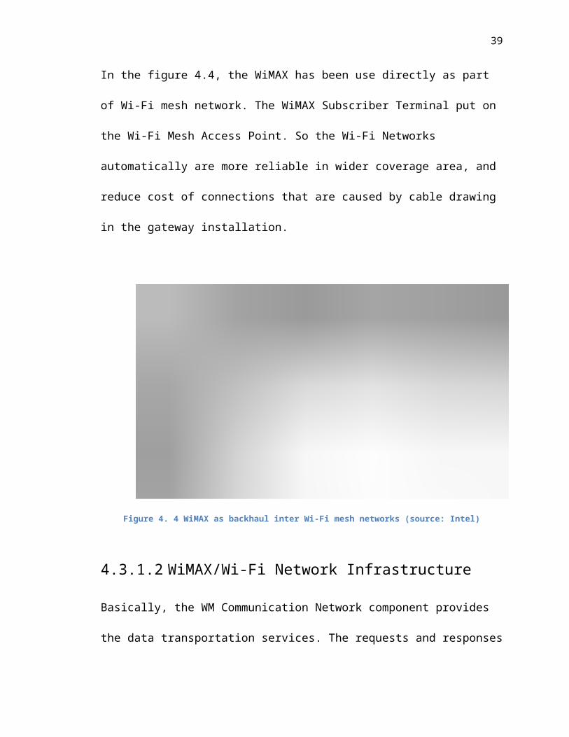
In the figure 4.4, the WiMAX has been use directly as part of Wi-Fi mesh network. The

WiMAX Subscriber Terminal put on the Wi-Fi Mesh Access Point. So the Wi-Fi

Networks automatically are more reliable in wider coverage area, and reduce cost of

connections that are caused by cable drawing in the gateway installation.

28

Figure 4. 4 WiMAX as backhaul inter Wi-Fi mesh networks (source: Intel)

4.3.1.2 WiMAX/Wi-Fi Network Infrastructure

Basically, the WM Communication Network component provides the data transportation

services. The requests and responses from Meter Data Center component and Wi-Fi

Smart Meter component will be delivered by the using to the transportation services of

WM Communication Network component.

The WM Communication Network component has three layers of network services like

the first three layers of the OSI model [22]:

29

Figure 4. 5 Logical view of the WM Communication Network includes the first three layers of the OSI model

The WM Communication Network is an integrated Wireless Mesh Network (WMN),

which uses Wi-Fi and WiMAX technologies [17]. The WM Communication Network has

the WiMAX Base Station, the WiMAX/Wi-Fi Gateway, and Wi-Fi Dual Band Mesh

Routers.

The figure 4.6 shows the physical model of the wireless mesh communication network.

The WiMAX Base Stations are connected to the Meter Data Center through wired

network. The Wi-Fi mesh routers are at the bottom level of the network hierarchy and can

connect with the Wi-Fi smart meters. Wi-Fi smart meters connect to the meter data center

via the hybrid WiMAX/Wi-Fi Communication Network.

30

Figure 4. 6 Physical model of the WM Communication Network. The network hierarchy includes the Wi-Fi Mesh Routers, the WiMAX/Wi-Fi Gateways, and the WiMAX BS.

31

4.3.1.3 Overview of NS-3 WiMAX Module

The NS-3 WiMAX model attempts to provide an accurate MAC and PHY level

implementation of the IEEE 802.16 specification with the Point-to-multipoint (PMP)

mode and the Wireless MAN-OFDM PHY layer. The WiMAX model composed of three

layers:

The MAC Convergence Sub layer (MAC-CS)

The MAC Common Part Sub layer (MAC-CPS)

The Physical (PHY) layer

The MAC Convergence Sub layer (CS)

The MAC-CS in this module implements the Packet CS, designed to work with the

packet-based protocols at higher layers. The CS is responsible of receiving packet from

the higher layer and from peer stations, classifying packets to appropriate connections (or

service flows) and processing packets. It keeps a mapping of transport connections to

service flows. This enables the MAC CPS identifying the Quality of Service (QoS)

parameters associated to a transport connection and ensuring the QoS requirements.

The MAC Common Part Sub layer (MAC-CPS)

The MAC Common Part Sub layer (CPS) is the main sub layer of the IEEE 802.16 MAC

and performs the fundamental functions of the MAC. The module implements the Point-

Multi-Point (PMP) mode. In PMP mode BS is responsible of managing communication

among multiple SSs. The key functionalities of the MAC-CPS include framing and

addressing, generation of MAC management messages, SS initialization and registration,

service flow management, bandwidth management and scheduling services.

Framing and Management Messages

32

The module implements a frame as a fixed duration of time, i.e., frame boundaries are

defined with respect to time. Each frame is further subdivided into downlink (DL) and

uplink (UL) sub frames. The module implements the Time Division Duplex (TDD) mode

where DL and UL operate on same frequency but are separated in time. A number of DL

and UL bursts are then allocated in DL and UL sub frames, respectively. Since the

standard allows sending and receiving bursts of packets in a given DL or UL burst, the

unit of transmission at the MAC layer is a packet burst. The module implements a special

Packet Burst data structure for this purpose. A packet burst is essentially a list of packets.

In the case of DL, the sub frame is simulated by transmitting consecutive bursts

(instances Packet Burst). In case of UL, the sub frame is divided, with respect to time,

into a number of slots. The bursts transmitted by the SSs in these slots are then aligned to

slot boundaries. The frame is divided into integer number of symbols and Physical Slots

(PS) which helps in managing bandwidth more effectively. The number of symbols per

frame depends on the underlying implementation of the PHY layer. The size of a DL or

UL burst is specified in units of symbols.

Network Entry and Initialization

The network entry and initialization phase is basically divided into two sub-phases, (1)

Scanning and synchronization and (2) Initial ranging. The entire phase is performed by

the LinkManager component of SS and BS.

Connections and Addressing

All communication at the MAC layer is carried in terms of connections. The standard

defines a connection as a unidirectional mapping between the SS and BS's MAC entities

for the transmission of traffic. The standard defines two types of connections: the

33

Management Connections for transmitting control messages and the Transport

Connections for data transmission. Note that each connection maintains its own

transmission queue where packets to transmit on that connection are queued. The

ConnectionManager component of BS is responsible of creating and managing

connections for all SSs.

Scheduling Services

The module supports the four scheduling services defined by the IEEE 802.16-2004

standard:

Unsolicited Grant Service (UGS)

Real-Time Polling Services (rtPS)

Non Real-Time Polling Services (nrtPS)

Best Effort (BE)

These scheduling services behave differently with respect to how they request bandwidth

as well as how the it is granted. Each service flow is associated to exactly one scheduling

service, and the QoS parameter set associated to a service flow actually defines the

scheduling service it belongs to. When a service flow is created the UplinkScheduler

calculates necessary parameters such as grant size and grant interval based on QoS

parameters associated to it.

WiMAX PHY Model

The Wireless MAN OFDM PHY specifications is implemented. This specification is

designed for non-light-of-sight (NLOS) including fixed and mobile broadband wireless

access. The proposed model uses a 256 FFT processor, with 192 data subcarriers. It

34

supports all the seven modulation and coding schemes specified by Wireless MAN-

OFDM. It is composed of two parts: the channel model and the physical model.

Channel model

When a physical device sends a packet (FEC Block) to the channel, the channel handles

the packet, and then for each physical device connected to it, it calculates the propagation

delay, the path loss according to a given propagation model and eventually forwards the

packet to the receiver device.

Physical model

The physical layer performs two main operations: (i) It receives a burst from a channel

and forwards it to the MAC layer, (ii) it receives a burst from the MAC layer and

transmits it on the channel.

Transmission Process: A burst is a set of WiMAX MAC PDUs. At the sending process, a

burst is converted into bit-streams and then splitted into smaller FEC blocks which are

then sent to the channel with a power equal P_tx.

Reception Process: The reception process includes the following operations:

1- Receive a FEC block from the channel. 2- Calculate the noise level. 3- Estimate the

signal to noise ratio (SNR) with the following formula. 4- Determine if a FEC block can

be correctly decoded. 5- Concatenate received FEC blocks to reconstruct the original

burst. 6- Forward the burst to the upper layer.

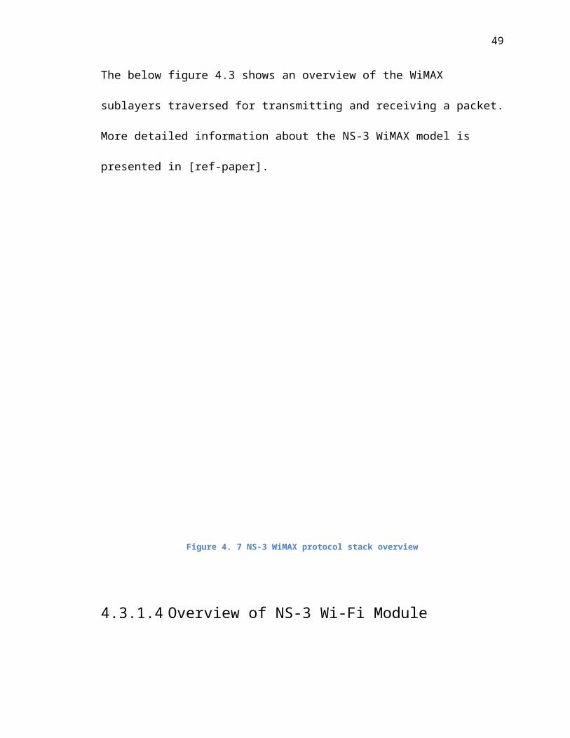
The below figure 4.3 shows an overview of the WiMAX sublayers traversed for

transmitting and receiving a packet. More detailed information about the NS-3 WiMAX

model is presented in [ref-paper].

35

Figure 4. 7 NS-3 WiMAX protocol stack overview

4.3.1.4 Overview of NS-3 Wi-Fi Module

The NS-3 802.11 model provides an accurate MAC-level implementation of the 802.11

specification and the PHY-level model of the 802.11a and 802.11b specifications.

There are four levels that were implemented in the current implementation:

The PHY layer model

The so-called MAC low models

The so-called MAC high models

A set of Rate control algorithms used by the MAC low models

36

The PHY layer implements a single 802.11a model in the ns3::WifiPhy class, and

recently extended to cover 802.11b physical layers.

The MAC low layer is split in 3 components:

ns3::MacLow takes care of RTS/CTS/DATA/ACK transactions

ns3::DcfManager and ns3::DcfState implement the DCF functions

ns3::DcaTxop and ns3::EdcaTxopN handle the packet queue, packet

fragmentation, and packet retransmissions.

The MAC high models contain the implementations for three Wi-Fi topological elements

– Access Point (AP) implemented in ns3::ApWifiMac, non-AP Station (STA)

implemented in ns3::StaWifiMac, and STA in an Independent Basic Service Set (IBSS)

implemented in ns3::AdhocWifiMac.

Rate control Algorithms include:

ns3::ArfWifiManager

ns3::AarfWifiManager

ns3::IdealWifiManager

ns3::CrWifiManager

ns3::OnoeWifiManager

ns3::AmrrWifiManager

ns3::CaraWifiManager

ns3::AarfcdWifiManager

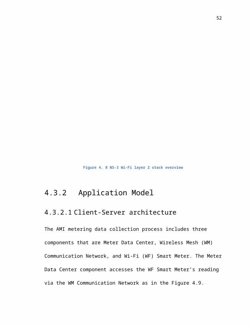
The below figure 4.4 shows the overview of the Wi-Fi L2 sublayers traversed for

transmitting and receiving a packet. More detailed information about the NS-3 Wi-Fi

model is presented in [ref-paper].

37

Figure 4. 8 NS-3 Wi-Fi layer 2 stack overview

4.3.2 Application Model

4.3.2.1 Client-Server architecture

The AMI metering data collection process includes three components that are Meter Data

Center, Wireless Mesh (WM) Communication Network, and Wi-Fi (WF) Smart Meter.

The Meter Data Center component accesses the WF Smart Meter’s reading via the WM

Communication Network as in the Figure 4.9.

38

Figure 4. 9 Smart meters access the Meter data center through the Wireless mesh communication network

4.3.2.2 Meter data traffic generation

Our current software simulates constant bit rate traffic. We allow users specifying the

starting time of packet streams. This allows for better network performance since the

packets from different nodes will not collide. It also helps debug the end to end

transmission and ensures that the network properly delivers the packets.

4.3.2.3 NS-3 Server application

An UDP protocol Server. It receives the meter messages.

4.3.2.4 NS-3 Client application

An UDP protocol Client. It sends the meter messages to the Server.

4.3.3 WLAN Simulation Design

4.3.3.1 Topology Configuration

Standard: Wi-Fi IEEE 802.11b

Connection mode: Infrastructure

Smart Meter (SM) at random position within the coverage area of the

corresponding AP

39

The Wi-Fi AP has the coverage range of 100 meters

Number of SMs: [1 – 100]

Wi-Fi link capacity: 11Mbps

4.3.3.2 Application Configuration

Server application is installed on the AP.

Client application is installed on SM.

Each Client application will send one meter message with 20 bytes length

to the Server application by using the Internet protocol UDP.

The Client application’s Data-Rate property is set to 20 bytes x 8 bits =

160bps = 0.160kbps

4.3.3.3 Simulation Planning

Repeatedly running the simulation scenarios with the different number of

SMs

Output: the network throughput, Tx Delay

4.3.3.4 Results Analysis and Conclusion

Calculate the average network throughput, Tx delay

Conclusion: Do the AP receive all of the messages from the SMs in 1

second?

4.3.4 WNAN Simulation Design


Standard: Wi-Fi IEEE 802.11a

40

Connection mode: Mesh

The Mesh Routers (MR) /Access Points (AP) are installed in the Grid

topology

o Distance between adjacent nodes (horizontal and vertical): 200

meters

Number of MRs/APs: [1 – 9]



Server application is installed on the Gateway (GW).

Client application is installed on APs.

Each Client application will send 100 messages, which have 20 bytes

length, to the Server application by using the Internet protocol UDP.

The Client application’s Data-Rate property is set to 100 x 20 bytes x 8

bits = 16000bps = 16kbps



MRs and APs

Output: the network throughput, Tx delay



Conclusion: Do the GW receive all of the messages from the APs in 1

second?

41

4.3.5 WMAN Simulation Design


Standard: WiMAX IEEE 802.16d

Connection mode: Point-To-Multipoint

The Subscribers (SS)/Gateways (GW) are installed in the grid topology.

Distance between adjacent nodes (horizontal and vertical): 1,000 meters

Number of SSs/GWs: [1 -10]

WiMAX link capacity: 4Mbps


Server application is installed on the Base Station (BS).

Client application is installed on SSs.

Client application will send 900 messages, which have 20 bytes length, to

the Server application by using the Internet protocol UDP.

The Client application’s Data-Rate property is set to 900 x 20 bytes x 8

bits = 144,000bps = 144kbps



SSs/GWs




42

Conclusion: Do the BS receive all of the messages from the SSs/GWs in 1

second?

4.3.6 WAN Simulation


Standard: Ethernet EEE 802.3

Connection mode: Point-To-Point

The BSs are connected to the Hub (or Data Center) in the Star topology

Number of BS: [1-20]

Ethernet link capacity: 10Mbps


Server application is installed on the Hub (or DC)

Client application is installed on BSs.

Client application will send 9,000 messages, which have 20 bytes length,

to the Server application by using the Internet protocol UDP.

The Client application’s Data-Rate property is set to 9,000 x 20 bytes x 8

bits = 1,440,000bps = 1.44Mbps



BSs



43


Conclusion: Do the DC receive all of the messages from the BSs in 1

second?

4.4 Implementing the Network Simulation

4.4.1 WLAN Simulation

4.4.1.1 NS-3 Script

Name: sm-ap-sim.cc

Description: This script implements the network model that simulates the

AMI meter data reporting process in a WLAN topology. The simulation

scenarios have one Wi-Fi Access Point (AP) and a number of the smart

meters (SM). The network devices are layout in a grid topology. The AMI

meter data reporting application will send the meter messages from the

SMs to the AP.

The source code of this script is in the Appendix session.

Syntax:

o Input:

nbSM - number of smart meter nodes to create [1]

duration - duration of the simulation in seconds [10]

verbose - turn on all WimaxNetDevice log components [false]

data-rate - packet data rate [0.160kbps]

statistic-start - the statistic is started at (second) [0]

44

o Output:

In every second:

Transmit (Tx) Packets, Receive (Rx) Packets, and

Maximum Tx Delay

In simulation period:

Average Transmit (Tx), Receive (Rx), and Transmit Delay

(TxDelay)

4.4.1.2 Linux Shell Script

Name: sm-ap-sim.sh

Description: Batch running the WLAN simulation application. This shell

script generates many WLAN simulation scenarios. Then it simulates the

scenarios, and logs the simulation results in the text files.

Syntax:

Input: none

Output: List of the log file names that store the simulation results

4.4.2 WNAN Simulation

4.4.2.1 NS-3 Script

Name: ap-gw-sim.cc


AMI meter data reporting process in a WNAN topology. The simulation

scenarios have one WiMAX/Wi-Fi gateway and a number of the mesh

45

routers. The network devices are layout in a grid topology. Some of the

mesh routers are configured as the APs. The AMI meter data reporting

application will send the meter messages from the APs to the gateway.


Syntax:

o Input:

x-size - number of columns of the grid [3]

y-size - Number of rows of the grid [3]

step - distance between two adjacent nodes (meter) [190]

access-points - number of Wi-Fi APs [1]

data-rate - packet data rate [20kbps]

statistic-start - the statistic is started at (second) [0]

o Output:

In every second:


Maximum Tx Delay



(TxDelay)


Name: ap-gw-sim.sh

46

Description: Batch running the WNAN simulation application. This shell

script generates many WNAN simulation scenarios. Then it simulates the


Syntax:

o Input: none

o Output:

List of the log file names that store the simulation results

4.4.3 WMAN Simulation

4.4.3.1 NS-3 Script

Name: gw-bs-sim.cc


AMI meter data reporting process in a WMAN topology. The simulation

scenarios have one WiMAX Base Station and a number of the Subscriber

Stations (or WiMAX/Wi-Fi Gateways). The network devices are layout in

a grid topology. The AMI meter data reporting application will send the

meter messages from the Subscriber Stations to the Base Station.


Syntax:

o Input:

nbSS - number of subscriber station to create [1]

scheduler - type of scheduler to use with the network devices [0]

47

duration - duration of the simulation (second) [10]


data-rate - packet data rate [144kbps]

statistic-start - statistic started at (second) [0]

o Output:

In every second:


Maximum Tx Delay



(TxDelay)


Name: gw-bs-sim.sh

Description: Batch running the WMAN simulation application. This shell

script generates many WMAN simulation scenarios. Then it simulates the


Syntax:

o Input: none

o Output: List of the log file names that store the simulation results

4.4.4 WAN Simulation

4.4.4.1 NS-3 Script

48

Name: bs-dc-sim.cc


AMI meter data reporting process in a MAN topology. The simulation

scenarios have one Hub and a number of the WiMAX Base Stations. The

network devices are layout in a star topology. The AMI meter data

reporting application will send the meter messages from the Base Stations

to the Hub node (or the Data Center).


Syntax:

o Input:

nbBS - number of base station to create [1]

duration - duration of the simulation (second) [10]


data-rate - packet data rate [1.44Mbps]

statistic-start - statistic started at (second) [0]

o Output:

In every second:


Maximum Tx Delay



(TxDelay)


49

Name: bs-dc-sim.sh

Description: Batch running the WAN simulation application. This shell

script generates many WAN simulation scenarios. Then it simulates the


Syntax:

o Input: none

o Output: List of the log file names that store the simulation results

Chapter 5Simulation Results and Analysis

5.1 Simulation Experiments

We has conducted four types of the network simulation experiments based on the type of

network topologies, including WLAN, WNAN, WMAN, and WAN topologies. We has

run each simulation experiment at least five times to compare the simulation results.

After the results were validated, the results from the last simulation were used to prepare

the input for a new simulation cycle of the parent network in the hierarchy. For example,

the WLAN simulation shows that there are 100 UDP packets transmitted in one second

from the SMs to the AP. Then, in the parent network, WNAN, the APs will be configured

to send the same number of packets received from the WLAN simulation, or 100 packets

in this example.

5.1.1 WLAN simulation experiment

The goal of the experiments is to evaluate the network throughput and the UDP packet

transmission delay with the different number of SMs in the WLAN topologies.

There are 11 experiments conducted to simulate the meter data traffic from the SMs to

the AP. The number of SMs is different between the scenarios, and between 1 and 100.

The location of the AP is fixed, but the location of the SMs were generated randomly in

51

each scenario. Based on the analysis of the Colorado Springs Utility network described

in Chapter 4, we observed there are average 50 SMs within 100x100 meter square area.

That is the reason we choose 50 as the number of SMs in a WLAN topology for the

simulation. The simulations results are shown and discussed in Section 5.3.1.

5.1.2 WNAN simulation experiment

The goal of the experiment is to evaluate the network throughput and the UDP packet

transmission delay with the different number of MRs and APs in the WNAN topologies.

There are 9 experiments conducted to simulate the meter data traffic from the APs to the

GW. The number of APs is different between the experiments, and from 1 to 9. The

network devices, GW and MRs/APs were installed in a grid topology with the distance

between nodes is 200 meters. GW position is at the left-top node. MRs/APs are installed

at other nodes of grid. The number of hops in a mesh routing path will increase with the

increasing number of the MSs/APs. The NS-3 mesh simulation module which we used in

this study limits the number of APs to nine. The simulations results are shown and

discussed in Section 5.3.2.

5.1.3 WMAN simulation experiment

The goal of the experiment is to evaluate the network throughput and the UDP packet

transmission delay with the different number of GWs in the WMAN topologies.

There are 10 experiments conducted to simulate the meter data traffic from the GWs to

the BS. The number of GWs is different between the experiments, and from 1 to 10. The

52

network devices, BS and GWs were installed in a grid topology with the distance

between nodes is 1,000 meters. BS position is at the left-top node. GWs are installed at

other nodes of grid. The NS3 WiMAX simulation module which we used in this study

limits the number of GWs to 20 but we have observed if the number of GWs increases

beyond ten, the packets will be lost.

Improve meter data transmission through packet aggregation

To improve the meter data transmission in the WMAN, we observed that the WiMAX

frame duration length is about 5 milliseconds that causes the maximum number of frames

processed in one second at a WiMAX/Wi-Fi gateway is about 200. It is not a good

utilization because there is only one meter data packet put in the sending UDP packet

during 5 ms of frame processing time. Instead, we can send more than one meter data

packets in one sending UDP packet by aggregating the received meter data packets at the

gateway into a single UDP packet and transmitting it with a WiMAX frame. For

example, in 5ms duration, the WiMAX connection with a transmission speed of 1Mbps

can deliver 5,000 bits or 625 bytes. If the length of the meter UDP packet is 20 bytes,

then the number of meter packets can be transmitted in one second is 31.

To evaluate the proposed improvement, we conduct simulation experiments , where 10

gateways connected to the base station in WiMAX point-to-multipoint mode. The

network performance is measured against the number of meter data packets put in a

WiMAX frame. The simulation parameter “number of meter data packets” increased until

the network is overloaded, or the number of received packets less than the number of sent

packets. The simulation results are shown and discussed in Section 5.3.3.

53

5.1.4 WAN simulation experiment

The goal of the experiments is to evaluate the network throughput and the UDP packet

transmission delay with the different number of BSs in the WAN topologies.

There are 7 experiments conducted to simulate the meter data traffic from the BSs to the

DC. The number of BSs is different between the experiments, and between 1 and 7. The

network devices, DC and BSs, were installed in a star topology. The connection between

DC and BS is Point-to-Point that simulates that optical fiber connection. To evaluate the

affect of the cable length to the transmission delay of a UDP packet, we conduct 11

experiments that have the cable length changed from 1km to 100km. The simulations

results are shown and discussed in Section 5.3.4.

5.2 Simulation Data Collection

Because the network infrastructure simulation process was divided into four sub-

networks such as WLAN, WNAN, WMAN, and WAN simulations. We can orderly

simulate and analyze each type of network topology. Therefore, we collected the

simulation results in each sub-network simulation. The simulation results were displayed

on the standard output device by the NS-3 C++ scripts. Four Linux shell scripts were

developed to run the simulation experiments many times for result validation. We has

modified the original standard output into the text file for offline further analysis.

5.3 Simulation Results

54

The following tables show the simulation results. The specification of the simulation

design, and the NS-3 simulation implementation are included in Chapter 4.

5.3.1 WLAN Simulation Results

5.3.1.1 Experiment 1: WLAN topology with 50 SMs

Topology configuration

Standard: Wi-Fi IEEE 802.11a

Connection mode: Infrastructure

The number of smart meters which the Wi-Fi AP serves: 50


Smart meter location: random position within the coverage area of the AP

NS3 SimulationTime in Sec

# of Tx Packets

# of Rx Packets Avg Tx Delay (µs)

# of Tx Packets / Meter

Total Processing Delay (µs)

1 0 0 0 1 02 0 0 0 1 03 50 50 36,011 1 36,0114 50 50 9,800 1 9,8005 50 50 10,025 1 10,0256 50 50 10,211 1 10,2117 50 50 9,418 1 9,4188 50 50 9,581 1 9,5819 50 50 9,164 1 9,16410 50 50 10,685 1 10,68511 50 50 9,587 1 9,58712 50 50 10,023 1 10,02313 50 50 9,993 1 9,99314 50 50 9,835 1 9,83515 50 50 10,038 1 10,03816 50 50 10,735 1 10,73517 50 50 9,701 1 9,70118 50 50 9,940 1 9,940

55

19 50 50 9,805 1 9,80520 50 50 11,209 1 11,209

Table 5. 2 WLAN simulation results with 50 SMs. The table shows the statistical data in every one second.

The first two second periods of the simulation were in the initialization phase of the Wi-

Fi network infrastructure mode. In the initialization period, there were no data sent in the

first two seconds. Moreover, the third second period shows that the average delay to be

36,011 µseconds. This is due to the Wi-Fi nodes need to resolve the AP’s IP address

before they send the UDP meter data packets to it. Otherwise, the average delay is

converged to about 10,000 µseconds.

5.3.1.2 Summary of conducted WLAN simulation experiments

# of Meters

# of Tx Packets

# of Rx Packets

Avg. Tx Delay (µs)

# of Tx Packets / meter


1 1 1 156 1 15610 10 10 1,420 1 1,42020 20 20 3,127 1 3,12730 30 30 5,326 1 5,32640 40 40 7,479 1 7,47950 50 50 9,985 1 9,98560 60 60 12,367 1 12,36770 70 70 14,559 1 14,55980 80 80 16,866 1 16,86690 90 90 19,371 1 19,371100 100 100 21,132 1 21,132

Table 5. 3 WLAN simulations with different number of SMs. The statistical data on a row is the results of an simulation experiment.

5.3.2 WNAN Simulation Results

5.3.2.1 Experiment 1: WNAN topology with 9 APs

56

Topology Configuration

Standard: Wi-Fi IEEE 802.11s

Connection mode: Mesh


The Mesh Routers (MR) /Access Points (AP) are installed in a grid topology

Distance between adjacent nodes (horizontal and vertical): 200 meters

NS-3 Simulation Time in Sec

# of Tx Packets

# of Rx Packets

Avg Tx Delay (µs)

# of Tx Packets / APs


1 441 374 5,037 50 251,8392 450 405 8,031 50 401,5553 450 400 730 50 36,5184 450 412 3,718 50 185,8945 450 450 685 50 34,2396 450 265 4,959 50 247,9757 450 374 234,084 50 11,704,2168 450 303 189 50 9,4429 450 456 5,507 50 275,36310 450 450 224 50 11,20711 450 450 213 50 10,63612 450 450 227 50 11,36613 450 450 203 50 10,17114 450 450 198 50 9,89915 450 450 206 50 10,29516 450 450 208 50 10,39117 450 450 213 50 10,66518 450 450 198 50 9,88619 450 450 264 50 13,22320 450 450 219 50 10,96021 450 450 199 50 9,95922 450 450 191 50 9,53823 450 450 190 50 9,49024 450 450 251 50 12,55025 450 450 293 50 14,63726 450 450 290 50 14,47527 450 450 266 50 13,308

57

28 450 450 239 50 11,95029 450 450 246 50 12,28130 450 450 214 50 10,67731 450 450 152 50 7,59132 450 450 158 50 7,90133 450 450 130 50 6,47834 450 450 130 50 6,52435 450 450 277 50 13,85136 450 450 245 50 12,22937 450 450 240 50 12,01038 450 450 236 50 11,80939 450 450 236 50 11,78640 450 450 5,472 50 273,62041 450 450 146 50 7,28942 450 450 148 50 7,39643 450 450 146 50 7,28744 450 450 146 50 7,30845 450 450 2,828 50 141,38646 450 450 192 50 9,62147 450 450 192 50 9,60848 450 450 200 50 9,98049 450 450 191 50 9,53950 450 450 268 50 13,39051 450 450 176 50 8,82452 450 450 180 50 9,00153 450 450 179 50 8,93354 450 450 176 50 8,78955 450 450 243 50 12,12556 450 450 206 50 10,29757 450 450 190 50 9,49358 450 450 189 50 9,44059 450 450 192 50 9,61060 450 450 205 50 10,26661 450 450 2,937 50 146,84262 450 450 227 50 11,34863 450 450 231 50 11,55364 450 450 233 50 11,64065 450 450 231 50 11,53366 450 450 5,518 50 275,91267 450 450 246 50 12,30568 450 450 237 50 11,83569 450 450 233 50 11,63170 450 450 236 50 11,784

58

71 450 450 269 50 13,46772 450 450 170 50 8,48573 450 450 175 50 8,73174 450 450 164 50 8,19075 450 450 171 50 8,52676 450 450 1,340 50 66,99477 450 450 159 50 7,96078 450 450 161 50 8,06679 450 450 161 50 8,04980 450 450 165 50 8,24381 450 450 250 50 12,52282 450 450 214 50 10,69283 450 450 221 50 11,05084 450 450 215 50 10,74285 450 450 223 50 11,15186 450 450 2,877 50 143,87287 450 450 254 50 12,71788 450 450 244 50 12,18689 450 450 247 50 12,35490 450 450 254 50 12,71891 450 450 2,881 50 144,02692 450 449 156 50 7,80893 450 450 151 50 7,55994 450 450 149 50 7,44095 450 450 148 50 7,37896 450 450 173 50 8,66797 450 450 1,206 50 60,29898 450 450 128 50 6,39799 450 450 130 50 6,499100 450 450 130 50 6,479

Table 5. 4 Simulation results for WLAN 3x3 grid topology with nine APs. The table shows the statistical data in every one second.

The initialization phase of the Wi-Fi Mesh network in the simulation occurred in the first

nine seconds. The mesh routing protocol needs to construct the routing path between the

APs and the gateway before UDP packets can be delivered to the receiver or mesh

gateway. This explains why there were the lost packets in the network initialization

period.

59

Other observation is the big jump on the delay of packet transmission at some simulation

seconds, i.e. 40, 45, 66. That is due to the changing in the routing path of the mesh

network. The new routing paths have more hops than the former ones. As a result, the

delay time has rapidly increased with the hop number on the routing path [21].

In the first second period, the number of sent UDP packets was less than 450. That is due

to the schedule for starting of traffic applications. The start time of traffic applications on

the APs were extendedly shifted for the performance measurement. The traffic

applications that has the starting time shifted far away from the starting of the first

simulation second, could not send all 50 UDP packets in the first second as planning. As

a result, the total sent packets in the first second were less than 450.

The delay time was converged to 500 µseconds.

5.3.2.2 Summary of conducted WNAN simulation experiments

# of APs

# of Tx Packets

# of Rx Packets

Avg. Tx Delay (µs)

# of Tx Packets / APs


1 50 50 0 50 02 100 100 21 50 1,0363 150 150 29 50 1,4324 200 200 34 50 1,6965 250 250 64 50 3,2036 300 300 103 50 5,1627 350 350 113 50 5,6498 400 400 158 50 7,8799 450 450 496 50 24,800Table 5. 5 WNAN simulation results. The statistical data on a row is the results of an simulation experiment.

5.3.3 WMAN Simulation Results

5.3.3.1 Experiment 1: WMAN topology with 10 GWs

60


Standard: WiMAX IEEE 802.16d

Connection mode: Point-To-Multipoint

WiMAX link capacity: 4Mbps

The Subscribers (SS)/Gateways (GW) are installed in the grid topology

Distance between adjacent nodes (horizontal and vertical): 1,000

meters


# of Tx Packets

# of Rx Packets

Avg Tx Delay (µs)

# of Tx Packets / GW


1 0 0 0 180 02 0 0 0 180 03 0 0 0 180 04 0 0 0 180 05 0 0 0 180 06 0 0 0 180 07 1791 1782 5,315 180 956,7048 1800 1803 5,266 180 947,9649 1800 1803 5,312 180 956,07610 1800 1800 5,372 180 966,89811 1800 1802 5,348 180 962,59712 1800 1799 5,297 180 953,51713 1800 1797 5,305 180 954,90114 1800 1793 5,315 180 956,68915 1800 1802 5,315 180 956,61916 1800 1799 5,295 180 953,11117 1800 1804 5,290 180 952,21818 1800 1801 5,368 180 966,23619 1800 1802 5,277 180 949,81020 1800 1803 5,312 180 956,09121 1800 1798 5,394 180 970,94022 1800 1801 5,314 180 956,60423 1800 1798 5,297 180 953,54124 1800 1797 5,369 180 966,49525 1800 1796 5,311 180 955,962

61

26 1800 1800 5,333 180 959,90027 1800 1802 5,382 180 968,78428 1800 1805 5,228 180 941,10829 1800 1800 5,237 180 942,59530 1800 1803 5,383 180 968,973

Table 5. 6 Simulation results for WMAN point-to-multipoint topology with ten GWs. The table shows the statistical data in every one second.

There were no packets sent in the first six seconds as planning because of WiMAX

network initialization period. The number of sent packets in the seventh second was less

than 1,800 as planning because of the shifted starting time of traffic applications.

The IEEE 802.16d standard has the frame time of 5 milli-seconds [31]. As a result, the

maximum number of WiMAX frames that can be sent in one second, is 180. The average

delay time of a UDP packet is close to the standard frame time.

5.3.3.2 Summary of conducted WMAN simulation experiments

# of GWs

# of Tx Packets

# of Rx Packets Avg. Tx Delay (µs)

# of Tx Packets / GW


1 180 180 5,147 180 926,5092 360 360 5,158 180 928,5043 540 540 5,171 180 930,7434 720 720 5,166 180 929,8965 900 900 5,161 180 928,9346 1080 1080 5,159 180 928,6437 1260 1260 5,166 180 929,8838 1440 1440 5,158 180 928,5139 1620 1620 5,229 180 941,18110 1800 1800 5,321 180 957,790

Table 5. 7 WMAN simulation results. The statistical data on a row is the results of an simulation experiment.

5.3.3.3 Summary of conducted experiments for the WMAN improved design

# of Meter

# of Tx Packets

# of Rx Packets

Total of Tx

Total of Rx

Tx Delay (µs)

# of Tx Packets /

Total Processing

62

Data Packets / Tx Packet

Meter Data Packets

Meter Data Packets Gateway Delay (µs)

1 1,800 1,800 1,800 1,800 5,319 180 957,3372 1,800 1,800 3,600 3,600 5,320 180 957,6083 1,800 1,800 5,400 5,400 5,320 180 957,6084 1,800 1,800 7,200 7,200 5,348 180 962,6085 1,800 1,800 9,000 9,000 5,348 180 962,7146 1,800 1,800 10,800 10,800 5,349 180 962,8797 1,800 1,800 12,600 12,600 5,374 180 967,3638 1,800 1,800 14,400 14,400 5,375 180 967,4699 1,800 1,800 16,200 16,200 5,456 180 982,12010 1,800 1,800 18,000 18,000 5,456 180 982,12011 1,800 1,800 19,800 19,800 5,458 180 982,41912 1,800 1,800 21,600 21,600 5,481 180 986,61313 1,800 1,800 23,400 23,400 5,483 180 986,91214 1,800 1,800 25,200 25,200 5,483 180 986,98515 1,800 1,800 27,000 27,000 5,457 180 982,33016 1,800 1,786 28,800 28,576 5,418 180 975,15117 1,800 1,786 30,600 30,362 5,441 180 979,464

Table 5. 8 shows the of simulation results of an WMAN topologies experiments that have 10 gateways. The number of meter data packets (length of 20 bytes) put in a sending UDP packet was changed until the UDP packet is fragmented.

In the above experiment, the number of UDP packets sent in one second is very close to the maximum WiMAX frames can send in one second (about 200), that will cause the network being overloaded when the UDP packets fragmented. For example, the number of received packets is less than the number of sent packets when there are 16 or 17 meter data packets in a UDP packet.

5.3.4 WAN Simulation Results

5.3.4.1 Experiment 1: WAN (Star) topology with 3 BSs


Link capacity: 10Mbps

Medium Transmission Delay: 3.3 us/km for optical fiber, cable length is a

random number

63

BSs are connected to the Data Center in the Star topology

Distance between DC and BS: in range from 1 km to 100km

Connection mode: Point-to-point topology


# of Packets Tx

# of Packets Rx

Avg Tx Delay (µs)

# of Tx Packets / BS


1 0 0 0 1,800 02 5,400 5,397 293 1,800 527,4703 5,400 5,400 293 1,800 527,4704 5,400 5,400 293 1,800 527,4705 5,400 5,400 293 1,800 527,4706 5,400 5,400 293 1,800 527,4707 5,400 5,400 293 1,800 527,4708 5,400 5,400 293 1,800 527,4709 5,400 5,400 293 1,800 527,47010 5,400 5,400 293 1,800 527,47011 5,400 5,400 293 1,800 527,47012 5,400 5,400 293 1,800 527,47013 5,400 5,400 293 1,800 527,47014 5,400 5,400 293 1,800 527,47015 5,400 5,400 293 1,800 527,47016 5,400 5,400 293 1,800 527,47017 5,400 5,400 293 1,800 527,47018 5,400 5,400 293 1,800 527,47019 5,400 5,400 293 1,800 527,47020 5,400 5,400 293 1,800 527,470

Table 5. 9 Simulation results for WAN point-to-point connection based star topology with three BSs. The table shows the statistical data in every one second.

The initialization period is in first two seconds. From the third second, the WAN network

has the average delay at 293 µseconds. The star topology has the point-to-point

connections between data center and base stations. This WAN network can provide a

very high bandwidth.

64

5.3.4.2 Summary of conducted experiments for the WAN

optimized design

# of Base Stations

Tx Packets

Rx Packets

# of Meter Data Packets / Packet

Total Tx Meter Packets

Total Rx Meter Packets

Avg. Tx Delay (µs)

# of Tx Packets / BS


1 1,800 1,800 15 27,000 27,000 260 1,800 468,0702 3,600 3,600 15 54,000 54,000 291 1,800 524,5003 5,400 5,400 15 81,000 81,000 293 1,800 527,4704 7,200 7,200 15 108,000 108,000 293 1,800 527,4705 9,000 9,000 15 135,000 135,000 252 1,800 453,8146 10,800 10,800 15 162,000 162,000 248 1,800 447,2807 12,600 12,600 15 189,000 189,000 214 1,800 385,756

Table 5. 10 WAN simulation results. The statistical data on a row is the results of an simulation experiment.

Cable Length (km)

# of Tx Packets

# of Rx Packets

# of Meter Data Packets / Tx Packet

Total Tx Meter Data Packets

Total Rx Meter Data Packets

Avg. Tx Delay (µs)


1 1,800 1,800 15 27,000 27,000 6 10,69010 1,800 1,800 15 27,000 27,000 36 64,15020 1,800 1,800 15 27,000 27,000 69 123,55030 1,800 1,800 15 27,000 27,000 102 182,95040 1,800 1,800 15 27,000 27,000 135 242,35050 1,800 1,800 15 27,000 27,000 168 301,75060 1,800 1,800 15 27,000 27,000 201 361,15070 1,800 1,800 15 27,000 27,000 234 420,55080 1,800 1,800 15 27,000 27,000 267 479,95090 1,800 1,800 15 27,000 27,000 300 539,350100 1,800 1,800 15 27,000 27,000 333 598,750Table 5. 11 shows the of simulation results of the WAN topologies experiments that have one BS. The length of the optical fiber cable that connects the BS and the DC, was changed to evaluate the total processing delay at a BS.

5.4 Simulation Results Analysis

65

5.4.1 WLAN Results Analysis

The Figure 5.1 show the simulation results in every one NS-3 second for the WLAN

topology that has 50 smart meters. Fifty UDP packets that sent from fifty smart meters,

received at the AP with the average transmission delay of 10 ms.

We can see that, the delay time of a package and the total transmission delay converge to

10 millisecond.

2 4 6 8 10 12 14 16 18 20 220510152025303540455055

0

2,000

4,000

6,000

8,000

10,000

12,000

WLAN (IEEE 802.11a) w/ 50 SMs Simulation

Packets Tx Packets RxAvg Tx Delay (us) Total Processing Delay (us)

NS-3 Sim Seconds

Pack

ets

Tim

e (u

s)

Figure 5. 1 simulation results in every one second for the WLAN Infrastructure mode topology with one AP and fifty SMs in the network.

66

0 20 40 60 80 100 1200

20

40

60

80

100

120

0

5,000

10,000

15,000

20,000

25,000

WLAN (IEEE 802.11a) w/ variable SMs Simu-lation

Packets Tx Packets RxTotal Processing Delay (us)

SMs

Pack

ets

Tim

e (u

s)

Figure 5. 2 simulation results for the WLAN infrastructure mode topology. The number of SMs is assigned from the one to one hundred in the experiments to evaluate the changing of the total processing delay at the SMs.

Figure 5.2 shows the simulation results for the WLAN infrastructure mode topology. The

number of SMs is assigned from the one to one hundred in the experiments to evaluate

the changing of the total processing delay at the SMs. The number of the UDP packets

sent and received in every one second for the simulation duration versus the number of

the SMs in many different simulation scenarios. The total processing delay is also plotted

on the chart.

We can see that, the network has successfully transmitted the UDP packets in every one

second from the senders (or smart meters) to the receiver (or AP).

Moreover, we can see that the total processing delay increases linearly with the number

of smart meters. The total processing delay at one smart meter is below the one second

67

threshold when the number of smart meters in the WLAN topology is equal or less than

seventy.

5.4.2 WNAN Results Analysis

0 10 20 30 40 50 60 70 80 90 1000

50

100

150

200

250

300

350

400

450

500

0

50,000

100,000

150,000

200,000

250,000

300,000

WNAN (IEEE 802.11s Mesh) w/ 9 APs Simu-lation


NS-3 Sim Seconds

Pack

ets

Tim

e (u

s)

Figure 5. 3 simulation results in every one second for the WNAN 3x3 mesh topology with nine APs and one GW. AP sent 50 packets in every one second to the GW.

Figure 5.4 shows simulation results in every one second for the WNAN 3x3 mesh

topology with nine APs and one GW. AP sent 50 packets in every one second to the GW.

There are total 450 UDP packets sent to the GW in every second. The number of sent

68

and received UDP packets are equal in every second. We also see that, the total

transmission delay converge to 500 millisecond.

0 1 2 3 4 5 6 7 8 90

100

200

300

400

500

0

5,000

10,000

15,000

20,000

25,000

30,000

WNAN (IEEE 802.11s Mesh) w/ variable APs Simulation

Packets Tx Avg. Packets RxTotal Processing Delay (us)

APs

Pack

ets

Tim

e (u

s)Figure 5. 5 simulation results of the WNAN 3x3 grid topology with nine MRs and one GW in the network.

Figure 5.4 shows the simulation results for the WNAN 3x3 grid topology. There are nine

MRs and one GW in the network. The number of APs are assigned from the one to nine

in the experiments to evaluate the changing of the total processing delay at the APs.

The number of the UDP packets sent and received in every one second for the simulation

duration versus the number of the APs in many different simulation scenarios. The total

processing delay is also plotted on the chart.

69


second from the senders (or APs) to the receiver (or GW).

Moreover, we can see that the total processing delay increases rapidly with the number of

APs. The line of total processing time likes a parabolic arc. That is due to the increasing

hop count on the mesh routing path [12, 21]. The total processing delay at one AP for

sending fifty 20-bytes packets is below the one second threshold.

5.4.3 WMAN Simulation Results

5 10 15 20 25 30 351770

1775

1780

1785

1790

1795

1800

1805

1810

0

200,000

400,000

600,000

800,000

1,000,000

1,200,000

WMAN (IEEE 802.16d) w/ 10 GWs Simulation


NS-3 Sim Seconds

Pack

ets

Tim

e (u

s)

Figure 5. 6. simulation results of WMAN point-to-multipoint topology with one BS and ten GWs in the network. GW sent 180 packets in every one second to the BS.

Figure 5.5 shows the simulation results in every one second for the WMAN point-to-

multipoint topology. There are one BS and ten GWs in the network. GW sent 180 packets

in every one second to the BS. There are 1,800 UDP packets sent to the BS in every

second. The number of received packets are not exactly equal the number of sent packets

70

in every second. The difference between them is between -5 and 5 packets. If a packet

does not arrive in the same second, it will arrive in the next second. The average delay of

a packet that is about 5.5 milliseconds, can validate this hypothesis.

We also see that, the total transmission delay converges to 930 milliseconds.

0 1 2 3 4 5 6 7 8 9 100

400

800

1,200

1,600

2,000

920,000930,000940,000950,000960,000970,000980,000990,0001,000,000

WMAN (IEEE 802.16d) w/ variable GWs Simulation

Packets Tx Avg. Packets RxTotal Processing Delay (us)

GWs

Pack

ets

Tim

e (u

s)

Figure 5. 7 simulation results for the WMAN topology. The number of GWs are assigned from the one to ten in the experiments to evaluate the changing of total processing delay at the GWs.

In the Figure 5.6 , the number of the UDP packets sent and received in every one second

for the simulation duration versus the number of GWs for different simulation

experiments. The total processing delay is also plotted on the chart.


second from the senders (or GWs) to the receiver (or BS).

Moreover, we can see that the total processing delay is between 930 and 960

milliseconds. It does not increase with the number of the GWs. This is due to the

71

WiMAX network or 802.16d standard has a fixed frame time (5ms) that is independent to

the number of the subscribers.

Impact on the network performance by aggregating meter data

Figure 5.7 shows the simulation results for the WMAN point-to-multipoint topology from

many experiments. There was one BS and ten GWs in the network. GW sent 180 packets

to the BS in every second. The number of meter data packets put in a transmitted UDP

packet was assigned from the one to seventeen packets to evaluate the changing of total

processing delay at the BSs in the experiments. Figure 5.7 shows the improvement of

network performance when the number of meter data packets are aggregated in a

transmitted UDP packet or the length of loaded data in one WiMAX frame. The number

of meter data packet was increased until the network going to the overloaded state. As we

can see on the chart, when the number of meter packets is less than 16, the network

successfully transmitted all of the UDP packets. This is due to the sending UDP packet

that contains a designated number of meter data packets, is not fragmented in the

transmission. Moreover, the traffic application was programmed to send out in every

second the number of UDP packets that can be delivered completely by the network in

one second.

However, the network is overloaded when the number of embedded meter data packets is

equal or greater than 16. This is due to the UDP packets was fragmented in the

transmission. That caused number of received packets in one second less than the number

of sent packets. As a result, the average transmission delay of a packet was increased.

72

0 2 4 6 8 10 12 14 16 180

5,000

10,000

15,000

20,000

25,000

30,000

35,000

940,000945,000950,000955,000960,000965,000970,000975,000980,000985,000990,000

WMAN (IEEE 802.16d) w/ 10 GWs, various sub-packet lengths simulation

Packets Tx Packets RxTotal Sub Packet Tx Total Sub Packet RxTotal Processing Delay (us)

Number of meter data packets

Pack

ets

Tim

e (u

s)

Figure 5. 8. Impact on the network performance by aggregating meter data .

5.4.4 WAN Simulation Results

73

0 5 10 15 20 255,394

5,396

5,398

5,400

5,402

0

100,000

200,000

300,000

400,000

500,000

600,000

WAN (Star Topology) w/ 3 BSs Simulation

Packets Tx Packets RxAvg Tx Delay (us) Total Tx Delay (us)

NS-3 Sim Seconds

Pack

ets

Tim

e (u

s)

Figure 5. 9 simulation results in every one second for the WAN star topology with DC and three BSs in the network. BS sent 1,800 packets in every one second to the DC.

Figure 5.10 shows the simulation results in every one second for the WAN star topology.

There are one DC and three BSs in the network. The connection between the DC and BS

is point-to-point. BS sent 1,800 packets in every one second to the DC. There are total of

5,400 packets sent to the DC in every second. The number of sent and received UDP

packets are equal in every second. We also see that, the total transmission delay

converges to 520 milliseconds.

74

0 1 2 3 4 5 6 7 80

20,000

40,000

60,000

80,000

100,000

120,000

140,000

160,000

180,000

200,000

0

100,000

200,000

300,000

400,000

500,000

600,000

WAN (Star Topology) w/ various BSs simulation

Packets Tx Packets RxTotal Meter Packet Tx Total Meter Packet RxTotal Processing Delay (us)

BSs

Pack

ets

Tim

e (u

s)

Figure 5. 11 simulation results for the WAN star topology from many experiments.

Figure 5.12 shows the simulation results for the WAN star topology from many

experiments. The number of BSs was assigned from the one to seven to evaluate the

changing of total processing delay at the BSs in the experiments. The number of the UDP

packets sent and received in every one second for the simulation duration versus the

number of BSs for different simulation experiments. The total processing delay is also

plotted on the chart.


second from the senders (or BSs) to the receiver (or the data center).

Moreover, we can see that the total processing delay is independent from the number of

the BSs. This is due to the BSs were connected to the data center in the point-to-point

75

connections. The network can transmit over 180,000 meter data packets that sent from

seven BSs, and the total processing time at each BS is less than 600 milliseconds.

However, the average delay is affected by the distribution of the BSs around the data

center.

0 20 40 60 80 100 1200

5,000

10,000

15,000

20,000

25,000

30,000

0

100,000

200,000

300,000

400,000

500,000

600,000

700,000

WAN (Star Topology) w/ various cable lengths simulation

Packets Tx Packets RxTotal Meter Packet Tx Total Meter Packet RxTotal Processing Delay (us)

Cable Length

Pack

ets

Tim

e (u

s)

Figure 5. 13 simulation results for the WAN star topology with one DC and one BS. The length of the optical fiber cable was assigned from the one to 100 kilometers.

Figure 5.14 shows the simulation results for the WAN star topology from many

experiments. There was one DC and one BS in the network. BS sent 1,800 packets to the

DC in every second. The length of the optical fiber cable that connects the DC and BS

was assigned from the one to 100 kilometers to evaluate the changing of total processing

delay at the BS in the experiments. We can see that the total processing time was linearly

76

increased with the length of the optical fiber cables that connect the BSs and the data

center.

Chapter 6Lessons Learned

6.1 The Development of SG-WIP Planning Tool

SG-WIP web application is a Google Maps mashup. The developing process is followed

the steps Requirement Spec, Design Spec, Coding and Testing, Deployment.

One of the most challenges of the Web application development process is the debugging

task. The debugging web pages has to be opened in a Web browser that supports the

debugging tool, such as the Developer Tools in the Microsoft Internet Explorer.

However, the debugging tool of the Web browser can only debug the scripts that run on

the client machine, i.e. JavaScript. The Google Maps mashup SG-WIP uses PHP

language at the Web server and JavaScript at the client browser. When a web page is

running at the client browser, the server scripts of that web page has been executed on the

web server before it is sent to the browser. So the debugging tool at the web browser can

not be used for the server scripts. Because we can not interactively debug the server

scripts from the browser tools, we need to log the running information of the server

scripts for the program tracing. We also converted the PHP server pages into the

executable programs and ran them on the server to test and debug the server scripts much

easier.

Another difficulty is the collecting of the housing unit geographical locations for the

residential density analysis, and the street light poles geographical locations for the

78

planning of the wireless antennae. We have the helps of CSU to get needed infrastructure

information for planning the AMI communication network in the simulation process.

Although the infrastructure information collection was a sophisticate process because

there were constrains on the data release policy from CSU, the topology planning tool has

the real world geographical location of the housing units and the streetlight poles to

display and process. Thus, the simulation network model is designed closer to the real

world.

6.2 The Development of Smart Grid Simulation

Model

This thesis employed the modern wireless network technologies such as WiMAX and

Wi-Fi. Network simulation tools help the network researchers evaluating their solutions,

designing new network devices or communication protocols. We has used two network

simulation software NS-3 and NCTUns [25] in researching and developing the

WiMAX/Wi-Fi communication infrastructure for AMI.

NCTUns has a great GUI that allows visually building the network topologies,

simulating, and animating the network simulation. We used the NCTUns to quickly

construct the simulation scenarios in the thesis proposal development phase.

NS-3 was used to construct the complicated parameterized wireless network model in this

thesis. There are hundreds thousand of the wireless nodes (smart meters) simulated using

the NS-3 simulator. One of the greatest features of NS-3 is providing the programmable

79

network modules such as WiMAX, Wi-Fi, CSMA under the Object Oriented

Programming (OOP) style in C++ language.

However, NS-3 is still in developing phase. There are not much help documents

published. I have found a bug in the WiMAX module that limits the number of the

Subscriber Stations to under twenty nodes in any simulation scenario. More information

about this bug is following the URL:

http://www.nsnam.org/bugzilla/show_bug.cgi?id=1025

NS-3 is free and open source project. It has been quickly accepted and supported by the

network research community.

6.3 The Simulation Process in NS-3

6.3.1 Initialization Phase of the Wireless Networks

NS-3 wireless network models such as WiMAX, and Wi-Fi perform the Initialization

phase at the starting of simulation duration. The time length of the initialization phase is

dependent on the network type, for example, the WiMAX topology with one BS and ten

SSs needs six seconds.

The simulation experiment designs should take this fact into account when making

decision about the start time of the network traffic applications.

6.3.2 The bugs in the NS-3 source code

NS-3 is still in the development phase. Whether you like it or not, the bugs are existing in

the source code, and they will affect to your simulation experiments.

https://webmail.uccs.edu/Redirect/www.nsnam.org/bugzilla/show_bug.cgi?id=1025

80

As I mentioned about the bug in the WiMAX module, I has sent the bug report to the

authors of the WiMAX module and immediately received their responses.

However, the open source software like NS-3 has been rapidly developing and receiving

the supports from the network research and development community. When there is a

bug reported, there are hundreds of the researchers around the world who can help

solving it immediately. As a result, the open source software NS-3 simulator will be more

and more reliable and helpful.

Chapter 7Simulation Limitations and Future Work

The proposed network model is implemented as a parameterized simulator in NS-3.

There are many featured variables that were used as the input of the simulator, such as

number of network device nodes, distance between nodes, data rates, etc. However, there

are some limitations that were not modeled in the simulator, for example, the height of

the nodes, geographical locations.

7.1 Display the Simulation Results on the SGWIP

Planning Tool

In this thesis, the designed simulation scenarios are based on the analysis of the

household density in the service areas [reference paper]. Because the real world network

topologies are complicated, in the simulation, we used only one featured simulation

scenario designed for a specific kind of the network topology i.e. WAN, WMAN,

WNAN, and WLAN.

82

We can use our SGWIP planning tool to edit the network topologies, simulation the trial

topologies, and display the simulation results on the GUI display. Then, we can compare

the different planned topologies to select the better one.

The SGWIP planning tool can be extended to export the network topologies and planning

results including the placement of antennae as a file.

The NS-3 network model can be modified to accept an arbitrary network topology as an

input. The real world topologies can then be simulated with the NS-3 network model and

produce simulation results for further analysis.

7.2 Alternative Method for Application Traffic

Simulation

The alternative method for application traffic simulation is the sending packet at a

random time. The packets are randomly sent from the smart meters to the data center

through the communication infrastructure. When the packets are transmitted in the

communication infrastructure, they will be logged in the trace files on the intermediate

network nodes along the routing path.

One of the advantages of this traffic simulation method is the randomly sending time of

the packets, which makes the simulation closer to the real world. However, in the

complicated simulation scenarios, such as in this thesis, the alternative method needs

more computing resources such as CPU time for random number generation, memory

space, storage space for trace files.

83

7.3 Improve the Antenna Placement Algorithm

The antenna placement algorithm in the SGWIP application should take into account the

network availability property when it searches for the antenna position. For network

availability improvement, the antenna will cover not only the corresponding network

area, but also its neighborhood networks. If the antenna of a network is down, the

working antenna in one of the neighborhood network areas will become the

corresponding one.

7.4 Store the Real-time Meter Data in the Database

Management System (DBMS)

DBMS is needed to store the real-time meter data for efficient data access and

management. The real-time metering collection process may pass a large amount of

meter data to the DBMS in less than one second. It opens an opportunity for a research of

the DBMS for the real-time meter data. The possible solution can employ the real-time

DBMS technologies, and the distributed computing technologies.

7.5 Evaluate the Performance of the Network Model

with the AMI real-time Demand Response

Applications

84

Demand response is one of the important goals of the AMI deployment. In contrast to the

metering collection, the demand response supporting applications will request the meter

data from the data center for the consumer’s demand analysis. Then the demand response

applications can help the consumers optimize their energy usage. Although this subject is

out of the scope of this thesis, it can contribute to the AMI researcher community an

other interesting performance evaluation of the WMN WiMAX/Wi-Fi infrastructure.

Chapter 8ConclusionAMI is being implemented by many utilities around the world. AMI contributes the

benefits not only to the utilities but also to the consumers. AMI real-time meter data

collection can give the utilities and consumers the ability to access the real-time meter

data. Consumers are benefits from the sharing real-time meter data because they can

monitor and actively adjust their demand of electric, gas, and water to save money.

Utilities are benefits from the real-time meter data because they can use the real-time

meter data to improve the quality of load profile charts, and load prediction. So the

utilities can save the fuel usage of power plants and reduce the price of electricity.

Many utilities have implemented the AMI wireless infrastructures for collecting meter

data automatically. However, most of the deployed wireless infrastructure did not support

or have not supported yet the real-time meter data collection. The intervals for meter data

collection are typically higher than one minute. The current meter data collecting period

is often in the range between fifteen and forty five minutes.

One of the main contributions of this thesis is the development a methodology for

measuring the performance of the hybrid WiMAX/Wi-Fi communication infrastructure

for the real-time metering data collection. The second contribution is the development of

a software tool SG-WIP for planning and designing the AMI wireless infrastructure using

the real utility light poles and meters GIS data from the city of Colorado Springs,

Colorado. The third contribution is the development of a simulator SG-SIM to evaluate

86

the performance of the hybrid WiMAX/Wi-Fi AMI network. We proposed a

parameterized WiMAX/Wi-Fi network model and implemented it in the NS-3 platform.

Experiments were conducted using the network simulation process, including the WLAN

(Wi-Fi) simulation, the WNAN (Wi-Fi Mesh) simulation, the WMAN (WiMAX)

simulation, and the WAN (optical fiber point-to-point connection) simulation. The

simulation results show that the proposed WiMAX/Wi-Fi WMN infrastructure can

transport the meter data from 160,000 smart meters in the CSU service areas to the data

center in one second.

From the simulation result analysis, we can conclude that the high scalability property of

WiMAX/Wi-Fi WMN helps flexibly extend the coverage area of the AMI wireless

infrastructure without degrading the network performance.

This thesis provides the utilities an AMI wireless communication infrastructure solution

that employs the WiMAX/Wi-Fi WMN architecture for real-time metering data

collection. The proposed WiMAX/Wi-Fi infrastructure allows the utilities deploying an

AMI wireless communication infrastructure not only at low cost of installation and

maintenance but also with high performance, scalability, and security.

Bibliography

[1] U.S. Department of Energy, “Smart Grid”,

<http://www.oe.energy.gov/smartgrid.htm>

[2] U.S Department of Energy, “Smart Grid: An Introduction”,

<http://www.oe.energy.gov/SmartGridIntroduction.htm>

[3] “Smart Grid”, <http://en.wikipedia.org/wiki/Smart_grid>

[4] National Institute of Standards and Technology, “NIST Framework and Roadmap for

Smart Grid Interoperability Standards, Release 1.0”, Jan. 2010.

[5] National Energy Technology Laboratory white paper “Advanced Metering

infrastructure”, February 2008.

[6] Edward Chow, “Secure Smart Grids”, Department of Computer Science, University

of Colorado at Colorado Springs, 2009.

[7] IEEE Standard 802 Part 11: Wireless LAN Medium Access Control (MAC) and

Physical Layer (PHY) Specifications, 2007.

[8] IEEE Standard 802 Part 15.1: Wireless Medium Access Control (MAC) and Physical

Layer (PHY) Specifications for Personal Area Networks (WPANs), 2005.

[9] IEEE Standard 802 Part 16: Air Interface for Broadband Wireless Access Systems,

2009.

[10] IEEE, “Draft amendment: ESS mesh networking”, IEEE P802.11s Draft 1.00,

November 2006.

http://www.oe.energy.gov/SmartGridIntroduction.htm

http://www.oe.energy.gov/smartgrid.htm

88

[11] Prasant Mohapatra, “Wireless Mesh Networks”, Department of Computer Science

University of California, Davis.

[12] I. F. Akyildiz, X. Wang, and W. Wang, "Wireless Mesh Networks: A Survey,"

Computer Networks Journal (Elsevier), vol. 47, no. 4, pp. 445-487, Mar. 2005.

[13] Srini Krishnamurthy, “Smart AMI Network Solutions Enable the Smart Grid”,

ElectricEnergyOnline.com, <http://www.electricenergyonline.com/?

page=show_article&mag=55&article=395>

[14] MetroFi, <http://en.wikipedia.org/wiki/MetroFi>

[15] SkyPilot, <http://skypilot.trilliantinc.com>

[16] EkaNet, <http://www.ekasystems.com/ekanet.htm>

[17] “Understanding Wi-Fi and WiMAX as Metro-Access Solutions”, Intel Corporation

white paper, 2004.

[18] B. Liu, Z. Liu, and D. Towsley, "On the capacity of hybrid wireless networks", in

Proceedings of IEEE INFOCOM, Mar. 2003, vol. 2, pp. 1543-1552.

[19] S. Zhao and D. Raychaudhuri, "On the Scalability of Hierarchical Hybrid Wireless

Networks, Proceedings of the Conference on Information Sciences and Systems (CISS

2006), March 2006, pp. 711-716.

[20] S. Zhao, I. Seskar and D. Raychaudhuri, "Performance and Scalability of Self-

Organizing Hierarchical Ad-Hoc Wireless Networks," Proceedings of the IEEE Wireless

Communications and Networking Conference (WCNC'04), Atlanta, GA. March 2004,

pp. 132-137.

http://www.ekasystems.com/ekanet.htm

http://skypilot.trilliantinc.com/

http://en.wikipedia.org/wiki/MetroFi

89

[21] J. –H. Huang, L. -C. Wang, C. -J. Chang, “Wireless Mesh Network: Architecture

and Protocols”, chapter title “Architectures and Deployment Strategies for Wireless Mesh

Networks”, Springer 2008.

[22] “OSI Model”, <http://en.wikipedia.org/wiki/OSI_model>

[23] WiMAX community, <http://www.wimax.com>

[24] The Network Simulator Ns-3, <http://www.isi.edu/nsnam/ns/>

[25] NCTUns 6.0 Network Simulator and Emulator,

<http://nsl.csie.nctu.edu.tw/nctuns.html>

[26] “The Protocol Developer Manual for the NCTUns 6.0”, Network and System

Laboratory, Department of Computer Science, National Chiao Tung University, Taiwan

2010.

[27] S.M. Huang, Y.C. Sung, S.Y. Wang, and Y.B. Lin, “NCTUns Simulation Tool for

WiMAX Modeling,” Third Annual International Wireless Internet Conference, October

22 – 24, 2007, Austin, Texas, USA. (EI and ISI indexed, sponsored by ICST, ACM, and

EURASIP)

[28] N.B. Salem and J.-P. Hubaux, "Securing Wireless Mesh Networks," Wireless

Comm., vol. 13, no. 2, 2006, pp. 50–55.

[29] Michael Purvis, Jeffrey Sambells, and Cameron Turner, “Beginning Google Maps

Applications with PHP and Ajax”, Apress, 2006.

[30] Google Maps JavaScript V3,

<http://code.google.com/apis/maps/documentation/javascript/>

http://code.google.com/apis/maps/documentation/javascript/

90

[31] M.A. Ismail, G. Piro, L.A. Grieco, T. Turletti, “An Improved IEEE 802.16 WiMAX

Module for the NS-3”, SIMUTools ’10 Proceedings of the 3rd International ICST

Conference on Simulation Tools and Techniques, Article No. 63, 2010.

[32] J. –H. Huang, L. -C. Wang, C. -J. Chang, “Coverage and Capacity of A Wireless

Mesh Network”, in Proc. WirelessCom’05, Jun. 2005.

Appendix A SG-WIP User Manual

A.1 The Installation

A.1.1 System Requirements

Apache Web Server

PHP module

MySQL Server

A.1.2 The Database

The database is named “sgwip”. There is a user account name “sgwip” created for

accessing the database from the Web application “SG-WIP”. The “sgwip” account need

proper access permission to allow the Web application “SG-WIP” access the tables in the

database.

A.1.3 The SG-WIP Application

The URL of the SG-WIP for downloading is at

http://cs.uccs.edu/~gsc/pub/master/phuynh/src/sgwip.zip

The Web application SG-WIP is installed on the Apache Web server.

For example the application was install on the local web server as the following Linux

Fedora file system: /usr/share/sgwip

92

Figure A. 1 SG-WIP installed on the Apache web server

93

A.2 The GUI Operations

A.2.1 Open the main page

In the Web browser, open the following URL: http://scad.eas.uccs.edu/sgwip/wan.html

Figure A. 2 The home page of SG-WIP

http://scad.eas.uccs.edu/sgwip/wan.html

94

A.2.2 Generate the WAN topology for first times of viewing

Click the menu item “New”

Wait for the GUI being generated and displayed on the Google maps (this process

may take many seconds to finish the job)

Click the menu item “WAN”

Figure A. 3 WAN topology includes twelve WiMAX Base Stations

95

Note: To return back to the WAN topology in the current path of the topology

exploration

A.2.3 Generate the MAN topology for first times of viewing

Click on the corresponding rectangle from the WAN topology GUI. A rectangle is a

Google Maps overlay object that represents for a network topology.

Wait for the network topology GUI being generated and displayed on the Google

Maps (this process may take many seconds to finish the job)

Click the menu item “MAN”

Note: To return back to the MAN topology in the current path of the topology exploration

A.2.4 Generate the Neighborhood Area Network (NAN) for 1st times viewing

Figure A. 4 WMAN Topology includes WiMAX BS, and WiMAX/Wi-Fi Gateways.

96

Click on the corresponding rectangle from the MAN topology GUI. A rectangle is a



maps (this process may take many seconds to finish the job)

Figure A. 5 WNAN Topology includes WiMAX/Wi-Fi gateway, and Mesh routers/Access Points.

Click the menu item “NAN”

Note: To return back to the NAN topology in the current path of the topology

exploration

97

A.2.5 Generate the LAN topology for first times of viewing

Click on the corresponding rectangle from the NAN topology GUI. A rectangle is a



maps (this process may take many seconds to finish the job)

Figure A. 6 WLAN Topology includes Wi-Fi Access Point, and Smart meters.

Click the menu item “LAN”

Note: To return back to the LAN topology in the current path of the topology

exploration

98

A.2.6 Change the antenna location of a network devices

The antennae of the wireless network devices such as WiMAX basestation, WiMAX/Wi-

Fi gateway, or AP/Mesh Router can be re-located to a better place within the topology.

Click the menu item “On-Change-Antenna-Loc”

Click the changed Antenna

Navigate to the destination network topology where there is an hanging object such as

street light poles, or the housing/building unit.

Click the target hanging object to select a new location for the antenna.

Appendix BSG-SIM Simulator Running Examples

B.1 The WLAN Simulation[phuynh@scad ns-3.9]$ ./waf --run "examples/sg-sim/sm-ap-sim --nbSM=1 --statistic-start=4"Waf: Entering directory `/root/ns-allinone-3.9/ns-3.9/build'Waf: Leaving directory `/root/ns-allinone-3.9/ns-3.9/build''build' finished successfully (1.273s)1 0 0 0ns2 0 0 0ns3 1 1 6082144ns4 1 1 1540048ns5 1 1 1540048ns6 1 1 1540048ns7 1 1 1540048ns8 1 1 1540048ns9 1 1 1540048ns10 1 1 1540048nsAvg. Tx packets/second:1Avg. Rx packets/second:1Avg. Tx delay (milliseconds):1

[phuynh@scad ns-3.9]$ ./waf --run "examples/sg-sim/sm-ap-sim --nbSM=10 --statistic-start=4"Waf: Entering directory `/root/ns-allinone-3.9/ns-3.9/build'Waf: Leaving directory `/root/ns-allinone-3.9/ns-3.9/build''build' finished successfully (1.272s)1 0 0 0ns2 0 0 0ns3 10 10 66400682ns4 10 10 19814024ns5 10 10 19277024ns6 10 10 19915025ns7 10 10 20013025ns

100

8 10 10 19392024ns9 10 10 20553025ns10 10 10 20255025nsAvg. Tx packets/second:10Avg. Rx packets/second:10Avg. Tx delay (milliseconds):19

[phuynh@scad ns-3.9]$ ./waf --run "examples/sg-sim/sm-ap-sim --nbSM=100 --statistic-start=4"Waf: Entering directory `/root/ns-allinone-3.9/ns-3.9/build'[ 519/1090] cxx: examples/sg-sim/sm-ap-sim.cc -> build/debug/examples/sg-sim/sm-ap-sim_3.o[1090/1090] cxx_link: build/debug/examples/sg-sim/sm-ap-sim_3.o build/debug/examples/sg-sim/sg-onoff-application_3.o -> build/debug/examples/sg-sim/sm-ap-simWaf: Leaving directory `/root/ns-allinone-3.9/ns-3.9/build''build' finished successfully (4.568s)1 0 0 0ns2 0 0 0ns3 100 100 688476554ns4 100 100 197641136ns5 100 100 195392137ns6 100 100 199219136ns7 100 100 197660136ns8 100 100 197337137ns9 100 100 201163137ns10 100 100 201171136nsAvg. Tx packets/second:100Avg. Rx packets/second:100Avg. Tx delay (milliseconds):198

101

B.2 The WNAN Simulation[phuynh@scad ns-3.9]$ ./waf --run "examples/sg-sim/ap-gw-sim --data-rate=16kbps --time=30 --access-points=1 --x-size=1 --y-size=1 --interfaces=4 --step=300 --statistic-start=12"Waf: Entering directory `/root/ns-allinone-3.9/ns-3.9/build'Waf: Leaving directory `/root/ns-allinone-3.9/ns-3.9/build''build' finished successfully (1.247s)1 99 99 0ns2 100 100 0ns3 100 100 0ns4 100 100 0ns5 100 100 0ns6 100 100 0ns7 100 100 0ns8 100 100 0ns9 100 100 0ns10 100 100 0ns11 100 100 0ns12 100 100 0ns13 100 100 0ns14 100 100 0ns15 100 100 0ns16 100 100 0ns17 100 100 0ns18 100 100 0ns19 100 100 0ns20 100 100 0ns21 100 100 0ns22 100 100 0ns23 100 100 0ns24 100 100 0ns25 100 100 0ns26 100 100 0ns27 100 100 0ns28 100 100 0ns29 100 100 0ns30 100 100 0nsAvg. Tx packets/second:100Avg. Rx packets/second:100Avg. Tx delay (milliseconds):0

102

[phuynh@scad ns-3.9]$ ./waf --run "examples/sg-sim/ap-gw-sim --data-rate=16kbps --time=30 --access-points=4 --x-size=2 --y-size=2 --interfaces=4 --step=300 --statistic-start=12"Waf: Entering directory `/root/ns-allinone-3.9/ns-3.9/build'Waf: Leaving directory `/root/ns-allinone-3.9/ns-3.9/build''build' finished successfully (1.252s)1 396 380 103982400ns2 400 400 874410ns3 400 400 856410ns4 400 400 866410ns5 400 400 902410ns6 400 400 211025206ns7 400 400 41414ns8 400 400 41414ns9 400 400 41414ns10 400 400 41414ns11 400 400 894996ns12 400 400 41414ns13 400 400 41414ns14 400 400 41414ns15 400 400 41414ns16 400 400 1273064ns17 400 400 41414ns18 400 400 41414ns19 400 400 41414ns20 400 400 41414ns21 400 400 1223822ns22 400 400 41414ns23 400 400 41414ns24 400 400 41414ns25 400 400 41414ns26 400 400 1135480ns27 400 400 41414ns28 400 400 41414ns29 400 400 41414ns30 400 400 41414nsAvg. Tx packets/second:400Avg. Rx packets/second:400Avg. Tx delay (milliseconds):0 [phuynh@scad ns-3.9]$ ./waf --run "examples/sg-sim/ap-gw-sim --data-rate=16kbps --time=30 --access-points=6 --x-size=2 --y-size=3 --interfaces=4 --step=300 --statistic-start=12"Waf: Entering directory `/root/ns-allinone-3.9/ns-3.9/build'

103

Waf: Leaving directory `/root/ns-allinone-3.9/ns-3.9/build''build' finished successfully (1.272s)1 594 570 106987685ns2 600 600 1632058ns3 600 600 1441058ns4 600 600 1642057ns5 600 600 1837642ns6 600 372 205857651ns7 600 828 1639371823ns8 600 600 1255824ns9 600 600 1337824ns10 600 600 1255824ns11 600 600 3000281ns12 600 600 1382824ns13 600 600 2284941ns14 600 600 321064ns15 600 600 321064ns16 600 600 2713123ns17 600 600 1274290ns18 600 600 993955ns19 600 600 319412ns20 600 600 319412ns21 600 600 989117ns22 600 600 924711ns23 600 600 2113878ns24 600 600 319412ns25 600 600 319412ns26 600 600 2505356ns27 600 600 808770ns28 600 600 2939821ns29 600 600 318997ns30 600 600 318997nsAvg. Tx packets/second:600Avg. Rx packets/second:600Avg. Tx delay (milliseconds):1 [phuynh@scad ns-3.9]$ ./waf --run "examples/sg-sim/ap-gw-sim --data-rate=16kbps --time=30 --access-points=9 --x-size=3 --y-size=3 --interfaces=4 --step=300 --statistic-start=12"Waf: Entering directory `/root/ns-allinone-3.9/ns-3.9/build'Waf: Leaving directory `/root/ns-allinone-3.9/ns-3.9/build''build' finished successfully (1.272s)1 891 738 119623509ns2 900 901 1001745189ns

104

3 900 900 2325664ns4 900 900 2484352ns5 900 853 4331459ns6 900 420 207812067ns7 900 652 1639814429ns8 900 588 206033357ns9 900 918 210843707ns10 900 900 1398469ns11 900 900 2194660ns12 900 900 3773257ns13 900 900 3320283ns14 900 900 2380716ns15 900 900 832062ns16 900 900 4425319ns17 900 900 2087537ns18 900 900 3081115ns19 900 900 2029719ns20 900 900 1498443ns21 900 900 3893531ns22 900 900 2187714ns23 900 900 2989236ns24 900 900 955469ns25 900 900 1240705ns26 900 900 2895261ns27 900 900 2384426ns28 900 900 4603544ns29 900 900 821468ns30 900 900 853298nsAvg. Tx packets/second:900Avg. Rx packets/second:900Avg. Tx delay (milliseconds):2

105

B.3 The WMAN Simulation [phuynh@scad ns-3.9]$ ./waf --run "examples/sg-sim/gw-bs-sim --nbSS=1 --duration=30 --statistic-start=10"Waf: Entering directory `/root/ns-allinone-3.9/ns-3.9/build'Waf: Leaving directory `/root/ns-allinone-3.9/ns-3.9/build''build' finished successfully (1.291s)1 0 0 0ns2 0 0 0ns3 0 0 0ns4 0 0 0ns5 0 0 0ns6 0 0 0ns7 900 892 12140304ns8 900 901 11695508ns9 900 901 11917504ns10 900 902 12139374ns11 900 900 12139064ns12 900 901 12138628ns13 900 901 11916180ns14 900 891 11915853ns15 900 910 12137866ns16 900 892 12137472ns17 900 902 11915024ns18 900 900 12136936ns19 900 901 11914387ns20 900 901 11913951ns21 900 902 12136048ns22 900 900 12135696ns23 900 900 12135260ns24 900 901 12135034ns25 900 892 11912460ns26 900 901 11912276ns27 900 901 12134104ns28 900 902 12133794ns29 900 900 11689065ns30 900 901 11911061nsAvg. Tx packets/second:900Avg. Rx packets/second:900Avg. Tx delay (milliseconds):12 [phuynh@scad ns-3.9]$ ./waf --run "examples/sg-sim/gw-bs-sim --nbSS=5 --duration=30 --statistic-start=10"Waf: Entering directory `/root/ns-allinone-3.9/ns-3.9/build'

106

Waf: Leaving directory `/root/ns-allinone-3.9/ns-3.9/build''build' finished successfully (1.261s)1 0 0 0ns2 0 0 0ns3 0 0 0ns4 0 0 0ns5 0 0 0ns6 0 0 0ns7 4496 4463 12279339ns8 4500 4505 12278987ns9 4500 4505 12278635ns10 4500 4507 12193302ns11 4500 4502 12278141ns12 4500 4505 12277831ns13 4500 4505 12192456ns14 4500 4468 12277211ns15 4500 4495 12276859ns16 4500 4503 12191400ns17 4500 4509 12191090ns18 4500 4501 12275845ns19 4500 4504 12275661ns20 4500 4505 12190202ns21 4500 4510 12274873ns22 4500 4500 12052408ns23 4500 4503 12137719ns24 4500 4497 12188962ns25 4500 4466 12273801ns26 4500 4505 12051143ns27 4500 4505 12188032ns28 4500 4509 11913989ns29 4500 4500 12272561ns30 4500 4505 12272293nsAvg. Tx packets/second:4500Avg. Rx packets/second:4500Avg. Tx delay (milliseconds):12 [phuynh@scad ns-3.9]$ ./waf --run "examples/sg-sim/gw-bs-sim --nbSS=10 --duration=30 --statistic-start=10"Waf: Entering directory `/root/ns-allinone-3.9/ns-3.9/build'Waf: Leaving directory `/root/ns-allinone-3.9/ns-3.9/build''build' finished successfully (1.268s)1 0 0 0ns2 0 0 0ns3 0 0 0ns

107

4 0 0 0ns5 0 0 0ns6 0 0 0ns7 8991 8935 20416344ns8 9000 9007 20415908ns9 9000 9002 20415724ns10 9000 9024 20415372ns11 9000 9004 20415062ns12 9000 8994 20414626ns13 9000 8991 20414484ns14 9000 8951 20414132ns15 9000 9010 20413864ns16 9000 9007 20413470ns17 9000 9013 20413244ns18 9000 9007 20412892ns19 9000 9007 20412582ns20 9000 9010 20412314ns21 9000 9009 20412004ns22 9000 8999 20411694ns23 9000 8982 20411342ns24 9000 8998 20411116ns25 9000 8965 20410680ns26 9000 9009 20410496ns27 9000 9011 20410186ns28 9000 9013 20409792ns29 9000 9004 20409566ns30 9000 9010 20409214nsAvg. Tx packets/second:9000Avg. Rx packets/second:9000Avg. Tx delay (milliseconds):20

108

B.4 The WAN Simulation [phuynh@scad ns-3.9]$ ./waf --run "examples/sg-sim/bs-dc-sim --nbBS=3 --duration=10 --statistic-start=3 --data-rate=1.44Mbps"Waf: Entering directory `/root/ns-allinone-3.9/ns-3.9/build'Waf: Leaving directory `/root/ns-allinone-3.9/ns-3.9/build''build' finished successfully (1.261s)1 0 0 0ns2 27000 26943 2079999ns3 27000 27000 2079999ns4 27000 27000 2079999ns5 27000 27000 2079999ns6 27000 27000 2079999ns7 27000 27000 2079999ns8 27000 27000 2079999ns9 27000 27000 2079999ns10 27000 27000 2079999nsAvg. Tx packets/second:27000Avg. Rx packets/second:27000Avg. Tx delay (milliseconds):2

[phuynh@scad ns-3.9]$ ./waf --run "examples/sg-sim/bs-dc-sim --nbBS=5 --duration=10 --statistic-start=3 --data-rate=1.44Mbps"Waf: Entering directory `/root/ns-allinone-3.9/ns-3.9/build'Waf: Leaving directory `/root/ns-allinone-3.9/ns-3.9/build''build' finished successfully (1.266s)1 0 0 0ns2 45000 44905 2079999ns3 45000 45000 2079999ns4 45000 45000 2079999ns5 45000 45000 2079999ns6 45000 45000 2079999ns7 45000 45000 2079999ns8 45000 45000 2079999ns9 45000 45000 2079999ns10 45000 45000 2079999nsAvg. Tx packets/second:45000Avg. Rx packets/second:45000Avg. Tx delay (milliseconds):2

[phuynh@scad ns-3.9]$ ./waf --run "examples/sg-sim/bs-dc-sim --nbBS=10 --duration=10 --statistic-start=3 --data-rate=1.44Mbps"Waf: Entering directory `/root/ns-allinone-3.9/ns-3.9/build'Waf: Leaving directory `/root/ns-allinone-3.9/ns-3.9/build'

109

'build' finished successfully (1.265s)1 0 0 0ns2 90000 89810 2079999ns3 90000 90000 2079999ns4 90000 90000 2079999ns5 90000 90000 2079999ns6 90000 90000 2079999ns7 90000 90000 2079999ns8 90000 90000 2079999ns9 90000 90000 2079999ns10 90000 90000 2079999nsAvg. Tx packets/second:90000Avg. Rx packets/second:90000Avg. Tx delay (milliseconds):2

[phuynh@scad ns-3.9]$ ./waf --run "examples/sg-sim/bs-dc-sim --nbBS=15 --duration=10 --statistic-start=3 --data-rate=1.44Mbps"Waf: Entering directory `/root/ns-allinone-3.9/ns-3.9/build'Waf: Leaving directory `/root/ns-allinone-3.9/ns-3.9/build''build' finished successfully (1.264s)1 0 0 0ns2 135000 134715 2079999ns3 135000 135000 2079999ns4 135000 135000 2079999ns5 135000 135000 2079999ns6 135000 135000 2079999ns7 135000 135000 2079999ns8 135000 135000 2079999ns9 135000 135000 2079999ns10 135000 135000 2079999nsAvg. Tx packets/second:135000Avg. Rx packets/second:135000Avg. Tx delay (milliseconds):2

[phuynh@scad ns-3.9]$ ./waf --run "examples/sg-sim/bs-dc-sim --nbBS=20 --duration=10 --statistic-start=3 --data-rate=1.44Mbps"Waf: Entering directory `/root/ns-allinone-3.9/ns-3.9/build'Waf: Leaving directory `/root/ns-allinone-3.9/ns-3.9/build''build' finished successfully (1.271s)1 0 0 0ns2 180000 179620 2079999ns3 180000 180000 2079999ns4 180000 180000 2079999ns5 180000 180000 2079999ns

110

6 180000 180000 2079999ns7 180000 180000 2079999ns8 180000 180000 2079999ns9 180000 180000 2079999ns10 180000 180000 2079999nsAvg. Tx packets/second:180000Avg. Rx packets/second:180000Avg. Tx delay (milliseconds):2

Documents

cs.uccs.educs.uccs.edu/~gsc/pub/master/phuynh/doc/phuynhThesisV1.docx · Web viewThe SkyPilot’s mesh network solution combines standard-based Wi-Fi access with a high performance