Document de Travail - econ.iastate.edu

Propositions for the building of a quantitative Austrian modelling:an answer to Prof. Rizzo and to Prof. Vriend

Université Paris X-NanterreMaison Max Weber (bâtiments K et G)

200, Avenue de la République92001 NANTERRE CEDEX

Tél et Fax : 33.(0)1.40.97.59.07Email : [email protected]

Document de Travail Working Paper

2007-09

Rodolphe BUDA

EconomiX

Université Paris X Nanterre

http://economix.u-paris10.fr/

UMR 7166 CNRS

Propositions for the Building of a

Quantitative Austrian Modelling: An Answer

to Prof. Rizzo and to Prof. Vriend

Rodolphe Buda∗

Economix UMR 7166 CNRS, University of Paris 10†

April 1, 2007

∗The author would like to thank here the anonymous referee for his remarks and advises.†200, Avenue de la République, 92001 NANTERRE Cedex - FRANCE - Tel. : 01-40-

97-77-88 Fax.: 01-47-21-46-89 - e-mail : [email protected]

1

Summary

In this paper, we try to promote the building of a Quantitative Austrian Modelling(QAM). QAM must be viewed as a complementary quantitative prolongation of the Aus-trian methods and as a complementary approach to the already existing quantitative ap-proaches - especially we would like here to answer to the appeal of Prof. N.J.Vriend [61].As we explain it in the first part, our approach resulted from a critical view of the econo-metric procedures by Austrian methods and, from a theoretical instrumental study of theeconometric models. We define the main properties to quantitative approaches and espe-cially to the QAM. In the second part, we present QAM principles and equations (of theAUSTRIAN model), and justify it according to the classical Austrian point of view. TheQAM could be viewed as an answer to Prof. M.J.Rizzo [49] about the relationship betweenthe Praxeology and the Econometrics. Indeed, according to its properties, even if QAMwon’t be able to recreate any observable data, it could give a consistent pattern where theother quantitative approaches could fit. Especially, QAM could help, we hope so, to an-swer the question we asked about the quality of the econometric behavioral equations [8],in providing two levels of data, from where we could extract a relationship useful to correctobservable econometric data. QAM is in building.

Résumé

Ce papier propose de faire la promotion d’une modélisation autrichienne quantitative(en anglais QAM). Cette modélisation doit être considée comme un prolongement de laméthode autrichienne et comme une modélisation complémentaire de celles déjà existantes- en particulier, nous aimerions répondre ici à l’appel du Professeur N.J.Vriend [61].Comme nous l’expliquons dans la première partie, notre approche est autant le résultatd’une vision critique - basée sur la méthode autrichienne - des procédures économétriques,que d’une étude instrumentale des modèles économétriques. Cette étude nous a conduit àdéfinir les propriétés des approches quantitatives en générale et de la QAM en particulier.Dans la seconde partie, nous présentons les équations (du modèle AUSTRIAN) et les an-crages de la QAM à la tradition autrichienne. Nous mettons en évidence le lien qu’ellepermet d’établir entre la Praxéologie et l’Econométrie, répondant en cela, nous l’espérons,au souhait du Professeur M.J.Rizzo [49]. Bien qu’elle ne permette pas de retrouver de don-nées observables, la QAM peut fournir des résultats qui peuvent être rapprochés de ceuxobtenus par les autres méthodes quantitatives, en particulier l’économétrie. Ainsi, grâceà ses deux niveaux de résultats de simulation, la QAM devrait permettre de contribuerà améliorer la qualité des équations économétriques de comportement [8]. Cependant, letravail accompli n’est qu’une première étape.

Key-words : Austrian Economics - Agent-based Computational Eco-nomics - Methodological Individualism - Quantitative approaches - Econo-metrics - Micro-Macroeconomic Bridge

JEL Classification : B41, B53, C5, C63, C87, C88Austrian Classification : AE1, AE3, AE5, AE9, AE14

Propositions for the Building of a Quantitative Austrian Modelling 3

Contents

Summary / Résumé 2

Contents 3

List of Figures and Tables 4

0 - Introduction 5

I - The Critique of the Econometric Procedures 5

1. The computational tools of the Keynesian Method Approch 6a - Instrumental point of view of the econometric models 6

i - Large Scale (Multidimensional) Modelling 6ii - High Accuracy Calculation 7

b - The Fundamental Diagnostic of the econometric problem 7i - Lucas’ Critique 7ii - The Theoretical Neutrality of the Economic Algorithms 8

2. The Individualism Method Approach 9a - A Simulation-Experimentation approach of the problem 9

i - Simulation Market Models 9ii - Experiment Market System 10

b - A First Conclusion About the Limits of Calculation 11i - Generalization of the Simulation Market Model 11ii - Typology of Modelling Representations 12

II - An Austrian Answer to the Econometric Problem : the QAM 14

1. The Quantitative Approachs of Modelling 14a - The QPQM Approach and Classification of the Quantitative Modeling 14

i - An Absurd Approach to describe the Properties of Quantitative Models 14ii - Classification of Modelling 14

b - Relevance of the Quantitative Approach Translation 16i - Quantitative Translation of the Austrian Topics 16ii - The Links between Econometrics, QAM and Experiment 17

2. Presentation and Expected Contribution of The QAM 19a - AUSTRIAN model : a first release of the QAM 19

i - Equations of the Model 19ii - Future Developpement of the Model 22

b - The Parallel Use of AUSTRIAN with Econometrics 24i - Ceteris Paribus Assumption Examination 24ii - The Austrian Procedure of the Econometric Correction 25

III - Some Temporary Concluding Remarks 27

References 29

Appendix 1 - The SINGUL Model 35

Appendix 2 - Impossibility and Uselessness of QPQM’s Building 37

4 Rodolphe Buda, Economix UMR 7166 CNRS, University of Paris 10

List of Figures and Tables

Fig.1 - ECHANGE General Algorithm 11Fig.2 - From Tools Building to Instrumental Analysis 13Fig.3 - The Links Beetween the Different Approches 17Fig.4 - Proximity to the Reality and the EE-QAM-SE Use 19Fig.5 - Network Production Process 22Fig.6 - Providing Relationship Between Firms 22Fig.7 - Agent Communication Process in AUSTRIAN 23Fig.8 - An Austrian Econometric Correction Procedure 26

AUSTRIAN : An Essay of Quantitative Austrian Model 21SINGUL Model 35

Table 1: Typology of Modelling Representations 13Table 2: Quality Criteria of Quantitative Models and Theories 14Table 3: An Essay of Quantitative Techniques and Method’s Typology 15Table 4: Exhaustive Transactions Account 37Table 5: Transactions Duration (Thousand seconds) 38


0 - Introduction

During the seventies, the keynesian econometric modelling reached thetop level of its use, then since it decreased. The main way used by econo-metricians to solve the problem is obviously based on statistical ground.However, in a previous paper [8], we suggested that the solution should be torebuilt the behavioral econometric equation, in involving a methodologicalindividualism point of view. This paper describes the links we found betweenthe Econometric modelling and the Austrian Approach to get econometricequations better, and finally the track for the building of a quantitative mod-elling based on an Austrian approach.

The first part explains how we was led from an instrumental to an in-dividualism approach to analyze the econometric problem - during Pr.Rizzo[49] considered that Econometrics could be used to provide some quantitativehistorical results (or rules) to the Praxeology.

In the second part, we present the classification we obtained from thedifferent quantitative modelling methods, hence we built a new one - an Aus-trian one - we called Quantitative Austrian Modelling (QAM). We presentproperties and the expected results of such modelling, used in the same timewith econometrics. Pr.Vriend [60] wished that Austrian Economists andAgent-Based Computational Economics Economists to work together. Wehope QAM answer to these wishes.

I - The Critique of the Econometric Procedures

Our purpose was initially to get better econometric models. We firstlyconsider the problem of accuracy - so we worked to multidimensional mod-els - then we considered the problem of the specification of the behavioraleconometric equations. That implied we had to consider that problem ac-cording to a new point of view - different than statistical one. The indi-vidualism methodological point of view seemed to be appropriated to thispurpose. Such an approach already used by the Agent-based ComputationalEconomics [57]. However, our purpose - to get news specification of behav-ioral econometric equations - led us to analyze the problem according to apraxeological point of view. The final question was to conciliate the econo-metric models - aggregated - with the individual models ; in other words,the generalization of the individual procedures. Thus we presented a firstquantitative modelling typology.


1. The computational tools of the Keynesian Method Approch

The instrumental analysis of the econometric problem led us to a newquestion. Is the choice of algorithm neutral according to a theoretical pointof view ?

a - Instrumental point of view of the econometric models

An intuitive method to get econometric models better consists to dis-aggregate the sample1. We worked to multidimensional models - multi-periodical, multi-sectoral, multi-regional models2.

i - Large Scale (Multidimensional) Modelling

The disaggregation of the models involves that we encounter new instru-mental problems. When econometrician-developer has to manage large scalesample, he usually encounters problems of resource’s limits. When we de-velop multi-dimensional systems, we could think we only have to transposethe classical algorithms to all the dimensions of the model3. The resolutionof multi-dimensional models is longer than mono-dimensional one too4.

1- See [47, 2] for an overview of the computational method for macro-econometricmodels.

2- We indeed have built a multi-dimensional economic modelling software, SIMUL. Thetypical problems of the econometrics software implementation: SIMUL usually can quicklyestimate and solve multi-dimensional econometric equations systems. It only needs an in-struction for such an equation by equation according to Y r,s

t = Xr,st .ar,s + ε

r,st . SIMUL is

divided into some modules. Mainly, one module manages econometric estimation proce-dures, another manages the data bank and another manages the resolution of the systems.For an overview of SIMUL software, see [9, 12].

3- Unfortunately, the limits of resources, especially the data memory one, prevents thiseasy transposition. The developers already know, some languages don’t manage data-memory efficiently. Even if the memory of computers increases, the size of the data-memory of such language is limited to 640 Ko - e.g. : Turbo-Pascal. M.S.Khanniche &S.H.Yong had developed an algorithm ("A Solution to Memory Limit of DOS Based LargeFinite Element Programs", Advances in Engineering Software, 21, 1994, pp.99-112.), butwe have developed another one. We don’t explain here the algorithmic problems linkedto this program. See [13] and our paper "From hyper-matrix to vector: an AlternativeMethod to Manage DOS Data-Memory Shortage", Working Paper GAMA, University ofParis 10, 9 p., 2003.

4- So, we have developed new faster algorithms, which decreases the size of iterationsduring calculation. We especially developed an algorithm for two dimensional aggregationcalculation - see [12] and our paper "Two Dimensional Aggregation Procedure : An Alter-native to The Matrix Algebraic Algorithm", Working Paper GAMA, University of Paris10, 26 p., 2005.


ii - High Accuracy Calculation

Even if a very few of papers specify5 that problem, the econometrician-developer has to study the problem of accuracy calculation6 - to increaseaccuracy of the models7, even if this correction never would reach perfection.

From all these previous instrumental questions, a new question appears :Is the upper level of disaggregation should be the individual one ? However,that choice would not resolve our problem, because the individual and thedisaggregated equations should not be the same one.

b - The Fundamental Diagnostic of the econometric problem

i - Lucas’ Critique

The problem consists to ask the following general problem, already no-ticed by R.Lucas [36] : How to correct the behavioral econometric equation? The diagnostic we suggested [8] - a self-evident proposition in a sense -was, that econometric behavioral equations suffer of a lack analogical rep-resentation of the economic behavior. These equations are more aggregatedto correctly represent the actual economic behaviors8. Thus, we aimed ourwork at a better representation of the markets9. Even if the Lucas’s critiquewas not based on Austrian grounds, L.M.Lachmann [30] and then T.Basse[4] advised to introduce it into the Austrian topics, and more generally to

5- The Handbook of Computational Economics [2] don’t specify it, but let’s quoteM.E.Jerrell, "Interval Arithmetic for Input-Output Models with Inexact Data", Com-putational Economics, 1997, 10(1), pp.89-100.

6- We indeed know that the representation of the number by the computer - the famousfloating-point arithmetics - is imperfect. We developed a multi-precision arithmetics - theGNOMBR library software. See our paper "Macroeconomic Modelling Accuracy’s ControlTool : GNOMBR", Working Paper GAMA, University of Paris 10, aug., 21 p. (+ GNOMBRsoftware), 1996.

7- The main use of such arithmetics for macroeconomic or econometric models, is todecrease floating point error diffusion, but not to increase the number of significant digits ofresults. For a interesting overview of the computer’s arithmetics problem, see M.Daumas& J.M.Muller (Eds), Qualité des calculs sur ordinateur - vers des arithmétiques plus fiables?, Paris, Masson, Informatique, 1997, 164 p.

8- The econometric equations suffer of their of the weakness of explanation [18].9- Let’s quote the originally work of M.Allais [1] who have built a macro-account from

summing of micro-account, in using differential calculation. This work get very clearly abridge between the individual to the global level. However, we didn’t follow this path tobuilt a modelling independent to national account theory.


apply econometric procedures only to historical investigations10. M.J.Rizzo[49] and more recently, R.Batemarco [5] think that the gap between Theo-retical models and Econometric models could be resolved by praxeologicalmethod. Moreover, Econometrics could be used to give historical (but notprospective) economic rules and M.J.Rizzo (ibid.) think that Econometriccould help praxeological method to set its principles with their empirical(quantitative) results.

ii - The Theoretical Neutrality of the Economic Algorithms

Until the birth of computational economics [2, 57], the economic calcu-lation search and the mathematics search (especially the numerical analysis)were separated. But the assumption of algorithmic neutrality must be leftnow. Firstly, is there a continuum between the disaggregated level modelsand hypothetical individualized models ? - see [12]. Unfortunately, we knowthat paradoxically, the accuracy result of the econometrics models does notcontinuously increase when the disaggregation level increases. Thus, two as-sumptions: 1̊ that means that there is an optimal level of disaggregation ;or (not exclusively) 2̊ that means that we can’t keep the same specificationof the equations with the disaggregation level and the individual level.

Secondly, calculation of the solution needs some algorithms. Let’s con-sider now, we previously explained that we sometimes choose between algo-rithms, or we have to change algorithms according to technical difficulties.Is the choice of algorithm significant or not ? Does algorithm’s change implyanother solution ? It seems to be obvious that another algorithm shouldgive the same solution as the referent algorithm. It’s even one of the criteriaof the development of new algorithms. However, it seems that, in fact, themore complex is the level of representation of the model, the more importantis the choice of the algorithm11. The Austrian methodology gave us sometools of analysis of this problem ; especially the Austrian representation ofthe Market. We firstly aim our study at the building of a simulation modelof market. But we need to built an experimental model of market too toprovide a validation of the simulation results.

10- "[. . .] econometrics in fact can be a very helpful research tool for economists studyinghistorical events." [4].

11- We know that the solution of the equilibrium calculation by a centralized process isdifferent than a parallel (decentralized) one - see [44].


2. The Individualism Method Approach

a - A Simulation-Experimentation approach of the problem

We developed two complementary tools to simulate the market process.This path did’t led us to conclude directly. However we obtain some conclu-sions about the limits of calculation in economics.

i - Simulation Market Models

A first step [12] to build a market’s simulation model consists to representsome operators on a same market under imperfect competition12 withoutany auctioneer. That means that all agents can’t make their transactionsat the same time13. The main default of such these models was the poorrepresentation of the information flows, and the bargaining. Furthermore, itwas a model of pure exchange, without production14.

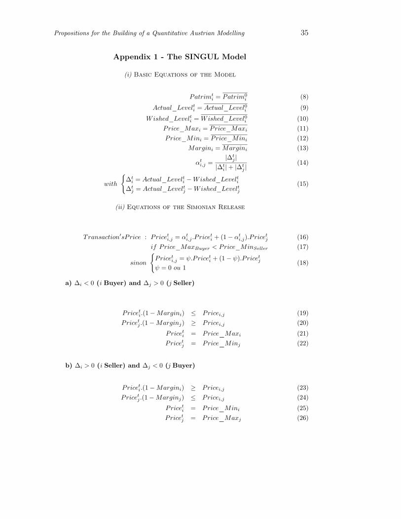
SINGUL is a very short period model with only one good. The agentscan’t keep quantities of this good over the level they indeed need. So, theycan’t speculate. SINGUL simulates the behavior of the N total numberof agents. For each agent SINGUL calculates the initial patrimony (1)- see complete equations set in Appendix 1 -, initial actual commoditieslevel (2), wished commodities level (3), "mind price" - it’s a kind ofhidden price : if the agent wants to buy the good, he won’t pay morethan a maximum price ; if the agent wants to sell the good, he won’tto be paid less than a minimum price - (4) and (5), and the negotiationmargin which determines the interval of transaction.The i-the agent meets a total number of Pi other agents. Their ranks areselected by random choice among N-1 ranks. The i-the agent negotiatesthe price of one unit of the good. At the beginning of the simulation, ifthe difference

∆ti = ActualLevelti −WishedLevelti

is negative, positive (resp.) then the agent is seller, buyer (resp.). Whenthe difference becomes equal to zero, then the agent leaves the market.

12- We developed MEREDIT based on the exchange of commodities and informationimperfection. See our paper "An Essay of Communication between Agents Modelling :MEREDIT", Working Paper GAMA, University of Paris 10, nov., (+ MEREDIT software),1994. We assumed false or true data endowment to be compared with a general true datamatrix. But we left this assumption because of its lack of subjectivism.

13- Iterations start from 1 to N where N represents the number of agents of the economy.14- We built another centralized and without auctioneer model. This one was without

information management, but with a better representation of goods supply, demand andbargaining, the model SINGUL [10]. Such a model was proposed according to a walriasiancomparison by P.Albin & D.K.Foley, "Decentralized, Dispersed Exchange Without anAuctioneer", Journal of Economic Behavior and Organization, 18, pp.27-51, 1992.


During the negotiation (9, 10) between the two agents i-the and j-the,they won’t be motivated with the same strength (given by the α param-eter).

αti,j =

|∆tj |

|∆ti| + |∆t

j |

Then price is calculated according to this difference of motivation15:

Priceti,j = αt

i,j .P riceti + (1 − αt

i,j).P ricetj

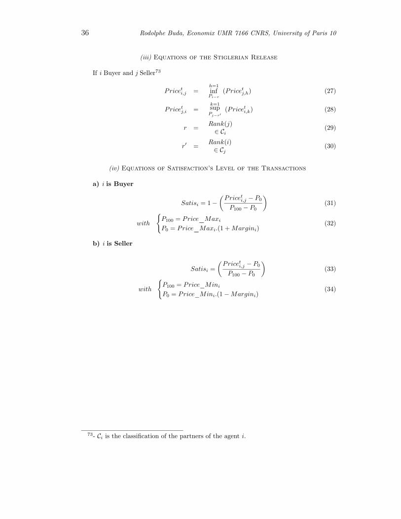
One of the two agents, who has got the greater difference, will acceptthe price condition of the other agent more easily. But the conclusion oftransaction happens only if the price belongs to both negotiation inter-vals. Neither agent knows the negotiation margin of his partner16. Themodel calculates to simulation run modes: a stiglerian one (agent meetsall his partner and chooses the best one, if reciprocity is true), and thesimonian one (agent deals with any partner, at each times the conditionsare filled).

Such simulation models can’t be validated by econometric procedures.Moreover, we would be wrong in trying to correct econometric equation withother econometric tools.

ii - Experiment Market System

Experimental validation appears to be the best one17. We present nowthe ECHANGE software [10, 13] designed to validate the SINGUL model.

ECHANGE software can (will be able to) run under two modes on a net-work system. The teacher e.g., can lead the system with the pilot modeand his pupils (or students) use operator mode but the pilot is not anauctioneer. ECHANGE simulates the transactions : the operator nor re-ally buys the goods neither do these goods really exist. The exchangestake place over a short period (we assume a daily period) and the goodshave been chosen among the leisure of the pupils.Each operator exists for the other one through his advertisement(s). Ateach period, the operator can write advertisements and/or answer to one(to buy and/or sell). They have to pay for information (advertisements).

15- Sometimes, the buyer’s "mind price" is greater than the seller one. We assume, onlyone of the two partners understands this fact and then agrees with the price of his partner.

16- The algorithm of partner’s choice is a Gale-Shapley one - See L.S.Gale & D.Shapley,"College Admissions and the Stability of Marriage", The American Mathematical Monthly,69(1), p.9-15, 1962.

17- Even if L.Mises [41] didn’t advise experiment in economics, V.L.Smith thinks theexperimental economics as it appeared in the sixties could be used according to Austrianeconomics methods "Experimental economics, created in the 50 years since Human Action,is kind to the Austrians in enabling us to demonstrate that the spontaneous order, operatingthrough property right institutions, exhibits the desirable characteristics that the Austriansclaimed for it." [54].


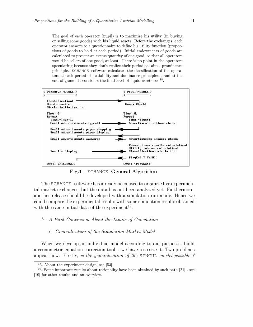
The goal of each operator (pupil) is to maximize his utility (in buyingor selling some goods) with his liquid assets. Before the exchanges, eachoperator answers to a questionnaire to define his utility function (propor-tions of goods to hold at each period). Initial endowments of goods arecalculated to present an excess quantity of one good, so that all operatorswould be sellers of one good, at least. There is no point in the operatorsspeculating because they don’t realize their periodical aim - prominenceprinciple. ECHANGE software calculates the classification of the opera-tors at each period - insatiability and dominance principles -, and at theend of game - it considers the final level of liquid assets too18.

Fig.1 - ECHANGE General Algorithm

The ECHANGE software has already been used to organize five experimen-tal market exchanges, but the data has not been analyzed yet. Furthermore,another release should be developed with a simulation run mode. Hence wecould compare the experimental results with some simulation results obtainedwith the same initial data of the experiment19.

b - A First Conclusion About the Limits of Calculation

i - Generalization of the Simulation Market Model

When we develop an individual model according to our purpose - builda econometric equation correction tool -, we have to resize it. Two problemsappear now. Firstly, is the generalization of the SINGUL model possible ?

18- About the experiment design, see [53].19- Some important results about rationality have been obtained by such path [21] - see

[19] for other results and an overview.


and by the way, how to introduce the production process ? Secondly, What arethe limits of calculation in economics ? This last question implies anotherquestion: For whom have we to make economic calculation ? There are threeanswers. The answer of macroeconomics is the State, the Austrian one isindividual (managers already make economic calculation), and the economicsearcher one is economic science could need it.

Economic calculation already exits at the individual level and built themarket itself. When agent uses this calculation procedure, he neither usesnor needs the whole information of the economy [25, 26]. As soon as we wantto get modelling with the whole information, we encounter problems withdata availability and treatment.

ii - Typology of Modelling Representations

According to the quantitative point of view, we have to aggregate themodel and/or the results. Thus we lose a lot of information. We encounterproblems with the census of the transaction20. Even if we would have gotthis information, or if we use representative sample data, we encounter arith-metics computer problem which decreases the accuracy of the results21. Ac-cording to the qualitative point of view, we have to decrease the complexity ofthe real world. Thus, some relationship would disappear during aggregations[43]. Especially, we encounter the famous Quételet paradox22. Furthermore,the aggregation is debatable, especially the homogeneity assumption23 [11].Thus, our temporary answer was, SINGUL-Generalized modelling was impos-sible. However, we’ll see in the second part, that the impossibility is actuallynot a complete one.

If we observe the evolution of economic calculation modelling - see Table 1-, we can notice that the first macro-econometric model’s builders developed

20- The data census problem is a human one too - see Appendix 2 and [48].21- About the quantitative problems, see Appendix 2 and our paper R.Buda (1996,

op.cit.).22- The new entity obtained after aggregation usually have no longer same properties as

his individuals. For a general point of view, see the Paradox of Quételet (1835) ; see tooC.W.J.Granger, "The Effect of Aggregation on Non-Linearity", Working Paper UniversityCalifornia San Diego, Aug., 1989, 25 p.

23- The products indeed are still transforming during the period of observation - thisproblem is known by statisticians when they try to calculate price indexes. This trans-formation can be slow or chaotic, but anyway the product is no longer the same from thebeginning to the end of the period. Such samples data of products can’t be aggregated be-cause, the homogeneity hypothesis is now wrong - exists inheritance relationship betweenthe different goods.


very aggregated and mono-computer procedures, then they progressively dis-aggregated them.

Table 1: Typology of Modelling Representations

Aggregation Level

Very Strong Weak No

Com

pute

rs

Mono-dimensional MultidimensionalOnly One Macro-econometric Macro-econometric -

Modelling Modelling

A Few Market Socialism (I) -

A Lot Of - Market Socialism (II) ACE, AL, QAM

One Per Agent - - Market itself (*)

(*) If we consider operators as calculators in the market.

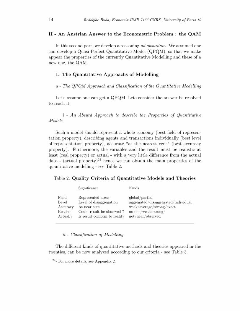
The Market socialism (I) - Lange-Lerner Model [32, 33, 34, 35] - andthen the Market Socialism (II) - Cockshott-Cottrell Model [15, 16, 17] -disaggregated and decentralized a lot the procedures. Finally, Agent-basedComputational Economics (ACE), Artificial Life (AL) [55] procedures andthe QAM we’ll present in the second part reach individual level of modellingwith a lot of computers - about our general approach, see Fig.2.

Fig.2 - From Tools Building to Instrumental Analysis


II - An Austrian Answer to the Econometric Problem : the QAM

In this second part, we develop a reasoning ad absurdum. We assumed onecan develop a Quasi-Perfect Quantitative Model (QPQM), so that we makeappear the properties of the currently Quantitative Modelling and these of anew one, the QAM.

1. The Quantitative Approachs of Modelling

a - The QPQM Approach and Classification of the Quantitative Modelling

Let’s assume one can get a QPQM. Lets consider the answer he resolvedto reach it.

i - An Absurd Approach to describe the Properties of QuantitativeModels

Such a model should represent a whole economy (best field of represen-tation property), describing agents and transactions individually (best levelof representation property), accurate "at the nearest cent" (best accuracyproperty). Furthermore, the variables and the result must be realistic atleast (real property) or actual - with a very little difference from the actualdata - (actual property)24 hence we can obtain the main properties of thequantitative modelling - see Table 2.

Table 2: Quality Criteria of Quantitative Models and Theories

Significance Kinds

Field Represented areas global/partialLevel Level of disaggregation aggregated/disaggregated/individualAccuracy At near cent weak/average/strong/exactRealism Could result be observed ? no one/weak/strong/Actually Is result conform to reality not/near/observed

ii - Classification of Modelling

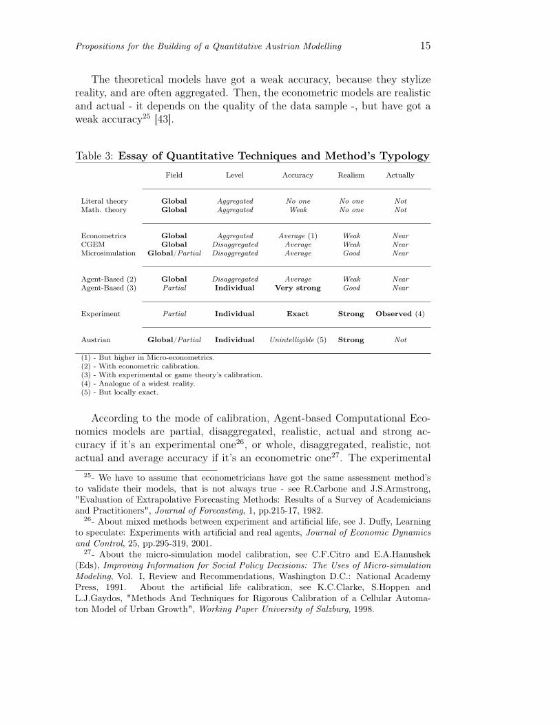
The different kinds of quantitative methods and theories appeared in thetwenties, can be now analyzed according to our criteria - see Table 3.

24- For more details, see Appendix 2.


The theoretical models have got a weak accuracy, because they stylizereality, and are often aggregated. Then, the econometric models are realisticand actual - it depends on the quality of the data sample -, but have got aweak accuracy25 [43].

Table 3: Essay of Quantitative Techniques and Method’s Typology

Field Level Accuracy Realism Actually

Literal theory Global Aggregated No one No one NotMath. theory Global Aggregated Weak No one Not

Econometrics Global Aggregated Average (1) Weak NearCGEM Global Disaggregated Average Weak NearMicrosimulation Global/Partial Disaggregated Average Good Near

Agent-Based (2) Global Disaggregated Average Weak NearAgent-Based (3) Partial Individual Very strong Good Near

Experiment Partial Individual Exact Strong Observed (4)

Austrian Global/Partial Individual Unintelligible (5) Strong Not

(1) - But higher in Micro-econometrics.(2) - With econometric calibration.(3) - With experimental or game theory’s calibration.(4) - Analogue of a widest reality.(5) - But locally exact.

According to the mode of calibration, Agent-based Computational Eco-nomics models are partial, disaggregated, realistic, actual and strong ac-curacy if it’s an experimental one26, or whole, disaggregated, realistic, notactual and average accuracy if it’s an econometric one27. The experimental

25- We have to assume that econometricians have got the same assessment method’sto validate their models, that is not always true - see R.Carbone and J.S.Armstrong,"Evaluation of Extrapolative Forecasting Methods: Results of a Survey of Academiciansand Practitioners", Journal of Forecasting, 1, pp.215-17, 1982.

26- About mixed methods between experiment and artificial life, see J. Duffy, Learningto speculate: Experiments with artificial and real agents, Journal of Economic Dynamicsand Control, 25, pp.295-319, 2001.

27- About the micro-simulation model calibration, see C.F.Citro and E.A.Hanushek(Eds), Improving Information for Social Policy Decisions: The Uses of Micro-simulationModeling, Vol. I, Review and Recommendations, Washington D.C.: National AcademyPress, 1991. About the artificial life calibration, see K.C.Clarke, S.Hoppen andL.J.Gaydos, "Methods And Techniques for Rigorous Calibration of a Cellular Automa-ton Model of Urban Growth", Working Paper University of Salzburg, 1998.


models are individual, with an exact accuracy, realistic and actual, but neverglobal. QAM is an individual - each individual is described -, global28,realistic - by experimental validation of the equations - but not actual -because we can’t calibrate the real-world parameters of economies29 :

"Economic equations describe only an imaginary condition that differsfrom the actual condition and that can never be realized." (L.von Mises[42])

globally unintelligible - because we don’t try to aggregate individual re-sults - but locally exact ones.

b - Relevance of the Quantitative Approach Translation

i - Quantitative Translation of the Austrian Topics

Austrian economics usually never uses mathematical (differential calcu-lation, statistics etc.) except arithmetics and logic. However, we think thatthe QAM could introduce a systematical use of arithmetics in the Austrianlogic analysis, especially to investigate its main topics (equilibrium, institu-tions, etc.). We’ll examine the original location of the QAM among the otherquantitative approaches.

QAM as an Austrian consistent deduction prolongation tool : Austrianeconomists usually deny the interest of the mathematical formulation in eco-nomic and social science [40, 24, 42]. However we think QAM follows theprinciples of Austrian economics. Indeed, QAM uses neither differential equa-tions nor econometric procedures. Furthermore, QAM must neither be usedto make predictive nor historical simulations. QAM exists to help investiga-tion of economic and social mechanisms described by the Austrian economics.QAM uses a lot of modules which simulates individual behaviors. Each mod-ule simulates an agent during its action - according to a praxeological pointof view. Each one indeed follows his own purpose (constitution of a basket ofcommodities, production of goods etc.) - according to the subjectivism prin-ciple. Each one looks for information and commodities in his environment incontacting other agent, during simulation - according to a catallaxical pointof view. A lot of demonstrations of L.Mises, F.Hayek or most of Austrian

28- In using an internet implementation, like the program of prime factorization of largeintegers led to test the safety of the RSA public key against the attempt of cracking [51].

29- ACE modelling implies a step of validation, by calibration - see M.C.Kathleen,"Validating Computational Models", Working Paper, Carnegie Mellon University, Sept.,1996, 40 p.


economists, are based on the logic30 but the conclusion is often undetermined:"... when the variable x increases, it involves the variable y decreases, but inthe same time the increase of z involves the increase of y, so that we can’tconclude.". We think that QAM could help the Austrian economists to leavesuch indetermination.

QAM as investigation tool of Austrian topics : Whatever the accuracydegree of the representation no model would be able to simulate the wholereality. Building a model means we have to choose to simplify some mecha-nisms or to hide some other considered (or assumed) insignificant. However,we think that QAM has reached an interesting level of individual represen-tation so that, QAM could help us to get a better understanding of marketmechanism, spontaneous order31, institutions genesis, hayekian productionprocess, or equilibrium tendencies32. QAM could help to show the mecha-nism of incitives during a market socialism procedures33. However, we thinkthat QAM interest is not only inside the Austrian economics thought.

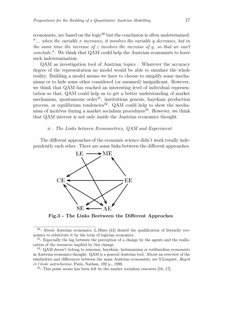
ii - The Links between Econometrics, QAM and Experiment

The different approaches of the economic science didn’t work totally inde-pendently each other. There are some links between the different approaches.

Fig.3 - The Links Beetween the Different Approches

30- About Austrian economics, L.Mises [41] denied the qualification of literarily eco-nomics to substitute it by the term of logician economics.

31- Especially the lag between the perception of a change by the agents and the reallo-cation of the resources implied by this change.

32- QAM doesn’t belong to misesian, hayekian, lachmannian or rothbardian economistsin Austrian economics thought. QAM is a general Austrian tool. About an overview of thesimilarities and differences between the main Austrian economists, see S.Longuet, Hayeket l’école autrichienne, Paris, Nathan, 192 p., 1998.

33- This point seems has been left by the market socialism renewers [16, 17].


The topic is obviously too large to be described into some words, but wecan highlight the following links between the different approaches. Literarilyeconomics (LE) appeared in antique era34 provides to the mathematical eco-nomics35 (ME) concepts, analysis or mechanisms which are mathematicallytranslated. Computational economics36 (CE) is mainly the discretization ofthe ME37. Our QAM (AE) is partially inherited from the CE and validatedby the experimental economics38 (EE). Especially, N.J.Vriend [62, 61, 59, 58]worked on the game theory design representation of markets. He has devel-oped some models based on hayekian principles (spontaneous order, infor-mation contagions, interactive adaptative agents) and wished that Austrianeconomists join ACE [60]. EE and econometrics39 (SE for statistical eco-nomics) are linked since the technical of simulation and experiment havebeen simultaneously used.

All approaches we recalled, however developed some methods indepen-dently each other. They sometimes have connections to progress, but theyare fundamentally independent according to their methods. Such an inde-pendence provides to each approach some validation tools from the otherone. In other words, the method of one approach could be relevant if themethod (an obviously independent one) of another approach gives the sameresult. That’s the reason why, we finally think that, as we’ll show it below,AE could help SE. Paradoxically, one of the main quantitative progress weassign to the QAM, is indeed the correction of the econometric behavioralequations.

Quantitative data and reality : For many reasons, the reality has beenand will never be completely "caught" by any modeler40. Even if modelerwould go into the field of his analysis, he could mistake or misunderstandan important data he however should have to keep. For example, a man iswalking on the street, which data we have to keep ? He comes from the marketand has just bought foods ; he falls on the street, the major is responsiblebecause, the floor was not safe, he saw advertising on a wall, and so on. Thissimple example shows us that, no quantitative modelling, could reach the

34- We could say that the LE was the initial form of economic science appeared underthe name of political economy.

35- Appeared between XVII and XIX-th centuries.36- Appeared at the end of the XX-th century.37- QAM isn’t such a discretization of mathematical economic theory.38- Appeared in the second part of the XX-th century.39- Appeared in the first part of the XX-th century.40- A subjectivist - [31] - bias exists into the observation of the modeler himself.


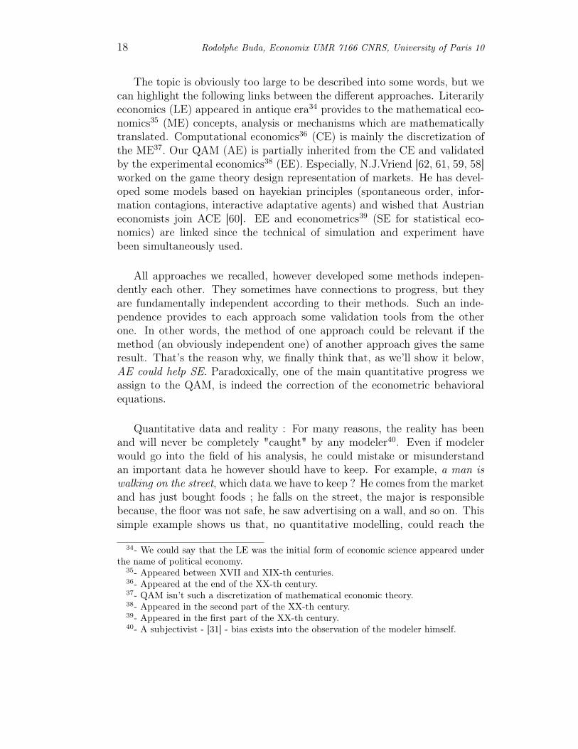
perfect level of realism. However, all approaches don’t suffer from this lackof realism according to the same degree - see Fig.4. The EE is obviouslythe nearest approach from the reality - but the observation is not exactlythe reality, only an analogy41. Then, because of it individual level and itscalibration according to statistical data, CE is the following nearest approachfrom the reality. QAM (AE) according to its individual modelling level,comes after in the reality’s proximity order, because we explained QAMdoes’nt try to describe directly the reality. Then SE because of its aggregationmodelling level, comes after. Finally, LE and ME because of their abstractionanalysis level, can’t represent observable facts.

Fig.4 - Proximity to the Reality and the EE-QAM-SE Use

2. Presentation and Expected Contribution of The QAM

a - AUSTRIAN model : a first release of the QAM

i - Equations of the Model

AUSTRIAN a total endogeneous individual model [14]: With SINGULmodel we did’nt resolve the endogeneouzed production problem ; SINGULwas only a commodities exchange simulation model. Given the productionprocess method, the question was the following : how to allocate factors toeach producer ? We had to leave the mathematical calibration. It would meanto solve a too big system of equations or to leave the global property. Wehad to leave experimental calibration too. It would mean to collect a too bigdata sample in a very quick time. Random calibration was left too, becausethe system would lose its coherence. We finally solved the system in startingit at the assumed earliest era of the Mankind. At the begin of the simulation,we indeed assumed that economy gets only a very short set of primary goods,

41- Unfortunately the reality that ME would try to describe could be different than theEE one. Moreover, about behavior, the link between EE and Economic Theory (EE-MEand EE-LE) is not an univoque one - see [52].


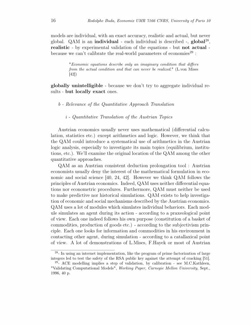
that each agent produces alone42. The dynamics of the system is given bythe differential ability of each agent. Each agent progressively produces moregoods than it needs so that, excess of goods for most of them appears. Thusthe conditions of exchange appeared. The main disadvantage of this way isthe probable long time to lead simulation to industrial economy. However, wedon’t try to simulate our actual economy. It’s more important to validate thebehavioral equation by experiment, than to validate the outcomes from theseequations. According to an individual level, it could be quasi impossible toget a simulation which would lead us to our real one43. The main advantageis the complete endogenous process of the simulation. The starting economyis a no monetary one, but progressively a common good is chosen to be themoney. In other words, after a lot of periods, the simulation should makeappear a money44. Hence the economy should become a monetary economy,after it was a barter economy. Furthermore AUSTRIAN simulates flows ofcommodities, payments and information ; the system itself creates it goods(a new combination of inputs gets a new good), money and information.

Description of the main equations45: AUSTRIAN is an individual levelsimulation model46. Each agent is a human being, not only a producer -producer eats every time, so he could be viewed as a consumer too -, notonly a consumer47. After the primary economic era, the simulation reaches anindustrial era where the number of goods is more important and productionorganization is developed. The endowment of the t period of simulation aregiven by the previous period48.

42- Each agent produces only one, two or three goods, among ten or twelve available inthe economy.

43- Given an economy of ten millions of people one million of goods, in doing such a simu-lation, we estimated the probability to reach our industrial state could be approximativelyto 1 per 101000000000, if we don’t try to reach each step - see Appendix 2.

44- The current simulation only run under a barter economy, but we assume that aparticular good could be choosen by agents, and become the money of the economy. Wehave to make simulation to answer definitively.

45- The following equations are not yet implemented into the current model, becausewe’re always working on the technical change problem.

46- The program is available. Contact me by e-mail.47- AUSTRIAN model, like the ACE Model [56], : starts at a primary ere of the economy,

but in AUSTRIAN model individuals are not assigned exclusively consumer or producer.48- In fact, it’s difficult to talk about period. During the large simulation, a lot of

computers will simulate each agent. The transactions between two agents will depend onthe availability of them. Each of them will live at least three different period during a day: leisure, work, sleep periods.


AUSTRIAN : An Essay of Quantitative Austrian Model

P jk =

D

infd=1

(

P jd

)

(1)

Ci =J

∑

j=1

αj · Pjk · Bj

i (2)

P ns =

E

infe=1

(

P ne

)

(3)

Wmz =

F

inff=1

(

Lmf

)

(4)

Vj =N

∑

n=1

βn · P ns · Bn

j +N

∑

n=1

γm · Wmz · Lm

j (5)

Pj = Vj + Fj (6)

Pb,s = ηb,s · Ps + (1 − ηb,s) · Pb (7)

Each agent looks for his own purpose. Consumers49 look for their best util-ity50 and managers for their best profit. During transactions, a process ofbargaining can appear - exchange is based on the subjective use-value givenby each agent to the commodities ([41],pp.119-26). At each period, consumeri tries to get a set of goods Bj

i - according to his own tastes51. Each con-sumer i tries to find the good at the lowest price. When consumer looks forBj, he compares prices of the D producers (or dealers) he can ask. Then hechooses the good Bj from k that price is lower (1). For each period, the costof consumption for the consumer i is given by (2). Each manager i tries toget maximum profit. When manager tries to produce the good Bj, he looksfor Kj

n capital-input and Ljm which are the lowest price. When manager con-

tacts the E providers of the Kn input, he chooses the s provider, which getshim lowest price input52 (3). According to the same ground, he chooses zworker among the F workers, which gives him lowest price labor (4). PriceP j of Bj that the manager get on his market is composed by cost-price V j

and profit margin F j - according to the management’s behavior (5) and (6).

49- We’ll use the terms of consumer and manager (resp.) but the correct term shouldbe individual as consumer and individual as manager (resp.).

50- We replaced the program Max U under income constraints with the programMin|Sc− Sd| under income constraints - Sc and Sd (resp.) for current stock and wishedstock (resp.). AUSTRIAN don’t simulates a general or a partial equilibrium a priori. TheAustrians don’t agree all on this question.

51- Each agent translates his own welfare by a specifical basket of good.52- Capital-input is evaluated per unit, and labor-input per worked hours.


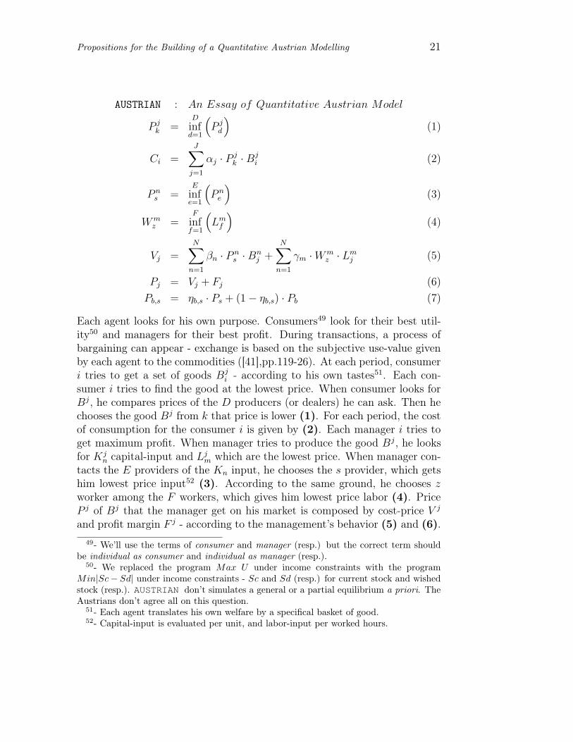
The bargaining process between buyer and seller (7) to determine the pricesis the same as the SINGUL model.

Fig.5 - Network Production Process

ii - Future Developpement of the Model

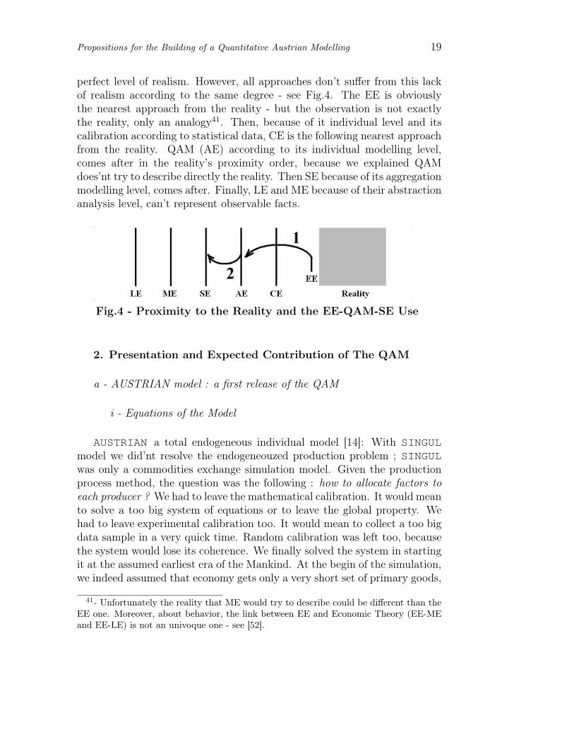
The technical change in the economy: The organization of production isgiven by a networks pattern. Firm is managed by a manager (M) - see Fig.5- who learnt or discovered a production process. Fig.5, his firm produces theoutput o from input three inputs i1, i2, i3 worked by two workers W1 and W2

(reps.) who receive wages w1 and w2 (reps.). Inputs come from the providingmarket PM1 and W2 and output is sold to customers market CM

53. Thetechnical change implies a new good or a change of process - complete one orjust a substitution of one or more of the inputs54. All the goods sold returna profit π to the manager.

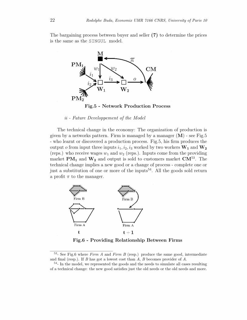
Fig.6 - Providing Relationship Between Firms

53- See Fig.6 where Firm A and Firm B (resp.) produce the same good, intermediateand final (resp.). If B has got a lowest cost than A, B becomes provider of A.

54- In the model, we represented the goods and the needs to simulate all cases resultingof a technical change: the new good satisfies just the old needs or the old needs and more.


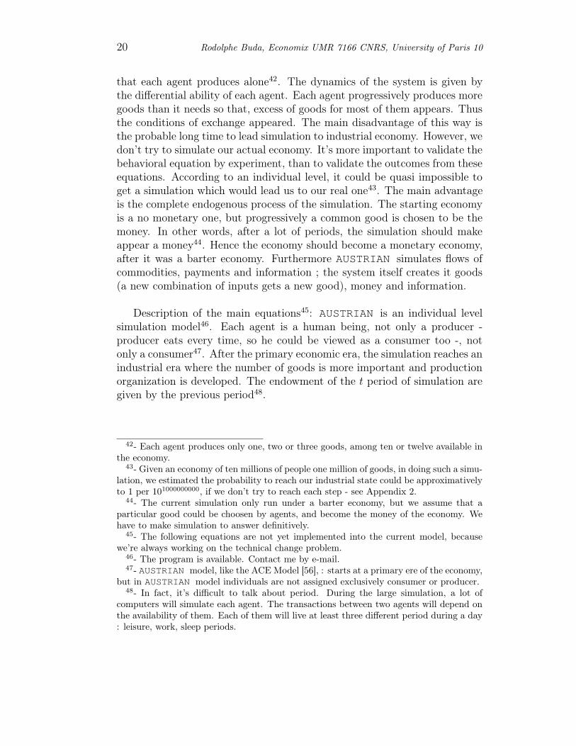
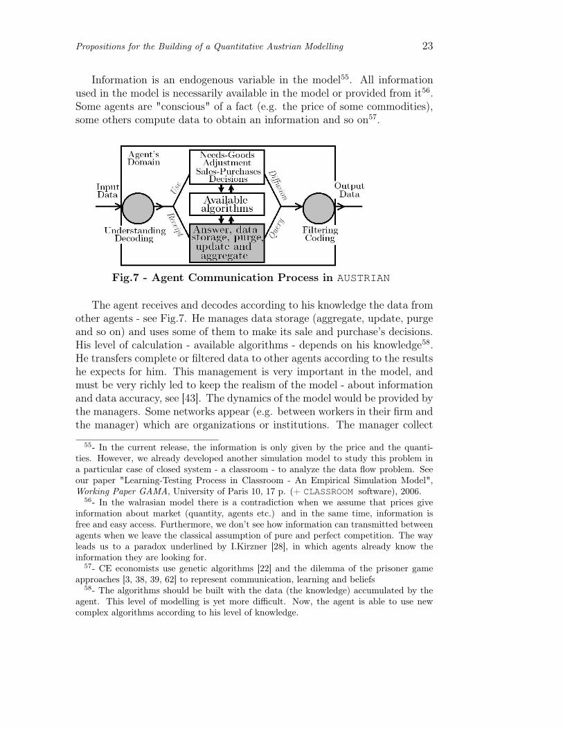
Information is an endogenous variable in the model55. All informationused in the model is necessarily available in the model or provided from it56.Some agents are "conscious" of a fact (e.g. the price of some commodities),some others compute data to obtain an information and so on57.

Fig.7 - Agent Communication Process in AUSTRIAN

The agent receives and decodes according to his knowledge the data fromother agents - see Fig.7. He manages data storage (aggregate, update, purgeand so on) and uses some of them to make its sale and purchase’s decisions.His level of calculation - available algorithms - depends on his knowledge58.He transfers complete or filtered data to other agents according to the resultshe expects for him. This management is very important in the model, andmust be very richly led to keep the realism of the model - about informationand data accuracy, see [43]. The dynamics of the model would be provided bythe managers. Some networks appear (e.g. between workers in their firm andthe manager) which are organizations or institutions. The manager collect

55- In the current release, the information is only given by the price and the quanti-ties. However, we already developed another simulation model to study this problem ina particular case of closed system - a classroom - to analyze the data flow problem. Seeour paper "Learning-Testing Process in Classroom - An Empirical Simulation Model",Working Paper GAMA, University of Paris 10, 17 p. (+ CLASSROOM software), 2006.

56- In the walrasian model there is a contradiction when we assume that prices giveinformation about market (quantity, agents etc.) and in the same time, information isfree and easy access. Furthermore, we don’t see how information can transmitted betweenagents when we leave the classical assumption of pure and perfect competition. The wayleads us to a paradox underlined by I.Kirzner [28], in which agents already know theinformation they are looking for.

57- CE economists use genetic algorithms [22] and the dilemma of the prisoner gameapproaches [3, 38, 39, 62] to represent communication, learning and beliefs

58- The algorithms should be built with the data (the knowledge) accumulated by theagent. This level of modelling is yet more difficult. Now, the agent is able to use newcomplex algorithms according to his level of knowledge.


all the time technical (which can update his own production technique: howto produce a particular good ?) and trade information (which help him tocalculate the better quantity and prices of his products)59.

Furthermore, we could represent justice problems. We could indeed sim-ulate robberies - transfer without any compensation of goods with a decreaseof the health capital of the victim -, murders - health capital of the victimdecreases to zero - and so on. This network could be observed also in termsof "rules" [27].

b - The Parallel Use of AUSTRIAN with Econometrics

i - Ceteris Paribus Assumption Examination

QAM is based on a massive parallel simulation. It means that eachagent is represented by an independent program which runs on a computer- SINGUL was a processional program. All computers are linked by a net-work60. At last, the choice of periodical step must be done very attentively.

"All such balances and statements are virtually interim balances and in-terim statements. They describe as well as possible the state of affairs atan arbitrarily chosen instant while life and action go on and do not stop.It is possible to wind up individual business units, but the whole systemof social production never ceases." ([41],p.214)61.

If we choose a too long periodical step then the simulation could be very long,if we choose a too short periodical steps, then the cohesion of the system isbroken. Now, the AUSTRIAN model is only implemented on mono-processorcomputer and can only simulate the primary economic ere.

QAM neither tries to make retro-simulations nor obtain whole results.QAM simulation must not be used like econometric one. It means, econo-metric simulation consists in testing the effect of the variation of a variableto the whole system, but, because of its endogenous form, such simulationis impossible with QAM. Furthermore, because of its inertia, when a largesimulation is running, we can’t stop it so easily like an econometric one. Thatimplies particular properties of its simulations.

We could indeed leave the ceteris paribus assumption usually used inthe econometric models. In using econometric and QAM models, we could

59- L.Lachmann [31] proposed to make difference between additive information andcomplementary information.

60- A LAN - Local Area Network - to test the model - or Internet to make the firstsimulation.

61- We underlined the idea we wanted to highlight.


better appreciate the actual weight of the ceteris paribus assumption. Wecould reach here the purpose of collaboration between Econometrics andPraxeology assigned by M.J.Rizzo [49].

ii - The Austrian Procedure of the Econometric Correction

Econometricians built models in choosing to link two or more variablesfrom a sample data observed at the same time of each variable. We describehere the classical method of the OLS - Ordinary Least Square62. Econometricequation simplifies reality and assumes some global regularities exist betweensocioeconomic variables followed by each agent (if we consider by examplethe cross series data). Unfortunately, each agent doesn’t follow exactly theglobal regularity represented by the estimated equation: the residuals vectorε will never be null, it’s impossible63 and unnecessary. So, the main pathof the Econometrics consists in finding new procedures to extract as muchinformation as possible from the residuals64. The problem becomes morecomplex as soon as the econometrician has to estimate simultaneously two(or more) equations into a model. That is the reason why one decided to con-sider economic variables like stochastic one and no more deterministic one65.Thus, econometric models became some virtual representation of reality. An-other problem proceeds from the quality of the data used in the econometricequations. Unfortunately, econometricians can’t control this point [43].

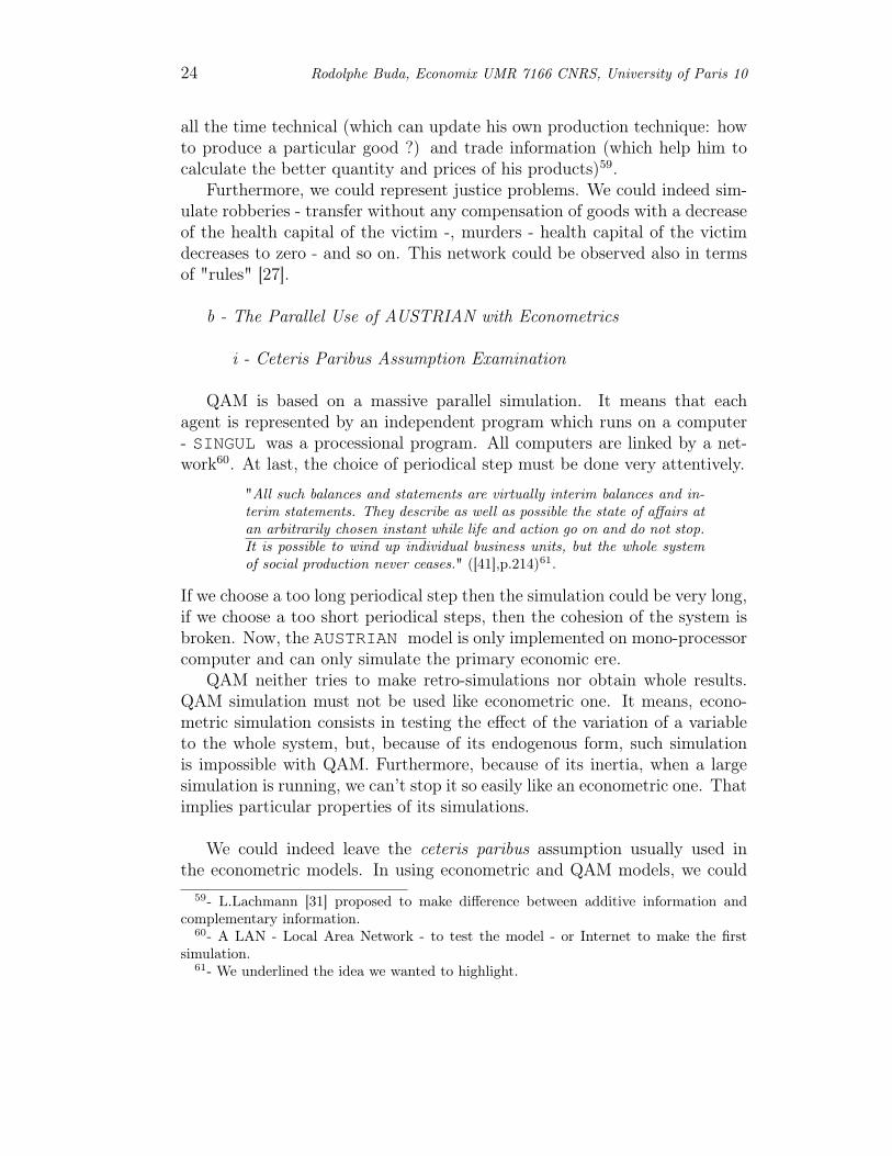
We think that QAM could help econometrician here. To achieve this pur-pose, we assume we make a large simulation with a QAM model (AUSTRIAN).At each simulation, the system is indeed able to provide two level of data66:the "systemic data" (parameters of the agents, level of stocks, currency, tasks,etc.) and the "endogenous data" (data that agent have exchanged together,true or false, complete or not, high frequency sampling or not, etc.)67. The

62- Given two variables Y and X observed at T periods (time series data) or observedfor N agents (cross series data), econometrician uses OLS method to calculate the bestequation which links the vectors Y and X. He finally obtain Y = a.X + ε where a is acoefficient and ε "keeps" the part of information of Y which is not explained by X.

63- The probability of a1 = a2 = . . . = aN can’t be equal to 100%.64- See R.Davidson & J.G.MacKinnon, Econometric Theory and Methods, Oxford, Ox-

ford University Press, 2004.65- A change introduced by T.Haavelmo [23] and studied by J.Marschak [37] too.66- The modeler who would try to study these data should choose a sample data but

could’nt study the complete data sample, supposed a large simulation.67- In a previous study, we describe the mechanism of a pedagogical software - OSCAR

for Outil de Simulation de Comptes A Reconstituer - devoted to the national accountteaching. The software would calculate some data from a sample of data and from some


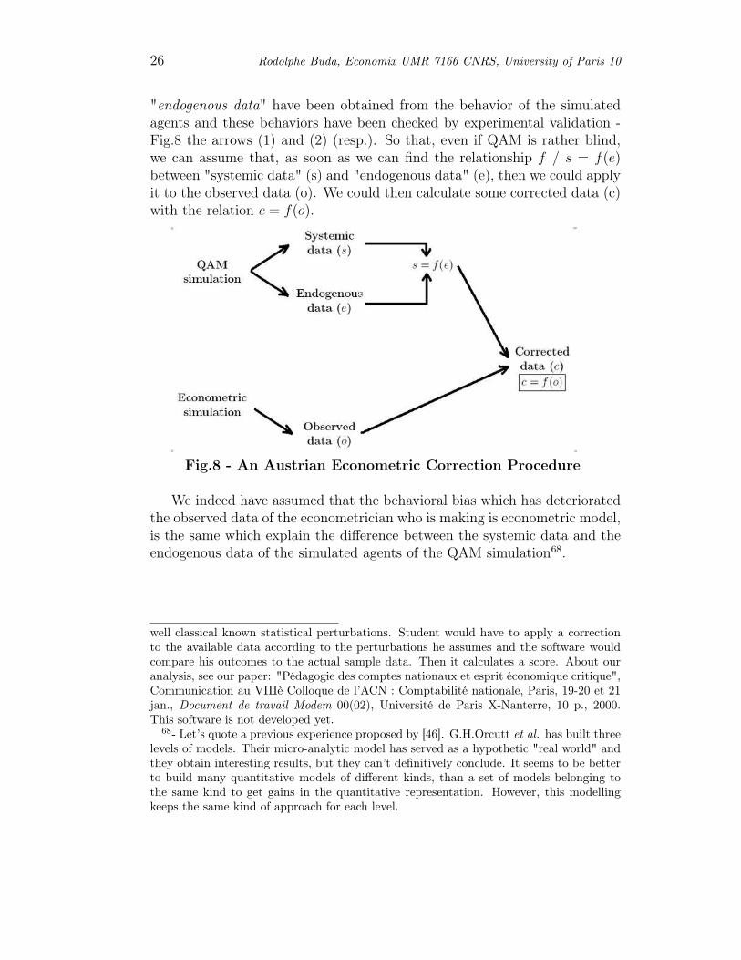
"endogenous data" have been obtained from the behavior of the simulatedagents and these behaviors have been checked by experimental validation -Fig.8 the arrows (1) and (2) (resp.). So that, even if QAM is rather blind,we can assume that, as soon as we can find the relationship f / s = f(e)between "systemic data" (s) and "endogenous data" (e), then we could applyit to the observed data (o). We could then calculate some corrected data (c)with the relation c = f(o).

Fig.8 - An Austrian Econometric Correction Procedure

We indeed have assumed that the behavioral bias which has deterioratedthe observed data of the econometrician who is making is econometric model,is the same which explain the difference between the systemic data and theendogenous data of the simulated agents of the QAM simulation68.

well classical known statistical perturbations. Student would have to apply a correctionto the available data according to the perturbations he assumes and the software wouldcompare his outcomes to the actual sample data. Then it calculates a score. About ouranalysis, see our paper: "Pédagogie des comptes nationaux et esprit économique critique",Communication au VIIIè Colloque de l’ACN : Comptabilité nationale, Paris, 19-20 et 21jan., Document de travail Modem 00(02), Université de Paris X-Nanterre, 10 p., 2000.This software is not developed yet.

68- Let’s quote a previous experience proposed by [46]. G.H.Orcutt et al. has built threelevels of models. Their micro-analytic model has served as a hypothetic "real world" andthey obtain interesting results, but they can’t definitively conclude. It seems to be betterto build many quantitative models of different kinds, than a set of models belonging tothe same kind to get gains in the quantitative representation. However, this modellingkeeps the same kind of approach for each level.


III - Some Temporary Concluding Remarks

QAM is ambitious because it needs to use a lot of computers through aparallel simulation69. But QAM is reasonable, because QAM calculation islimited to the representation of some potential economies.

AUSTRIAN model is in building70. Firstly, we now work on a betterspecification of the individual agent data-management - more exactly to thetranslation into equations. Secondly, we are looking for the better kind ofrelationship we should built between the systemic and the endogenous data.But this question depends widely on the answer of the previous question.

Anyway, we think that, QAM could help Austrian economists in theiranalyzes and investigations, and QAM would provide too a large storage oftwo-level data which could be analyzed by econometricians, to adjust theirown models and to reconciliate them with stylized theories - especially theycould leave the ceteris paribus assumption.

As individual level of modelling, QAM reinforces the micro-macro bridgeasserted (or assumed) by microeconomics but never improved, and seriouslyworked by the CE and would perhaps decrease the existing gap betweenAustrians and other economists - see [6, 7]. The "communication failurebetween the Austrians and other economists" ([6], p.44) could disappear if theAustrians would provide a quantitative answer to the quantitative questionof the other economists. On the other hand, we could compare outcomesfrom the game theory design of the ACE with these from QAM.

Now, about the question of the respective domain of the ACE and theQAM, it seems that we can say, QAM uses some tools of the ACE and seeksmainly the same purposes. In a sense, we can say that QAM belongs tothe ACE economic school. But, in another sense, QAM is not linked toequilibrium or games theory71 that could be better to the Austrian analysis.

69- Biologists and Mathematicians (resp.) have already such an experience of this pro-cedure to analyze DNA and Prime numbers (resp.) - see [51].

70- The current model AUSTRIAN is implemented in Turbo-Pascal 7.0 and don’t reachthe monetary and industrial step of the simulation. It run on only one computer. Moreoverthe final release will be implemented in Java and will turn on Internet.

71- Especially to the microeconomic formulation - see [20] about such a modelling.


Finally, we think that paradoxically, QAM could help Austrianeconomists in their investigations about the limits of calculation in economics,especially about the renewed debate of the socialism calculation. Even if cal-culation abilities have significantly increased with the current computers, thesocialist calculation renewers have not denied the problem of the incentives.QAM could help to investigate this question.


References

[1] Allais M., Les fondements comptables de la macro-économique - les équa-tions comptables entre quantités globales et leurs applications, Paris,PUF, Collection Dito, 96 p., 1954.

[2] Amman H.M., Kendrick D.A. & Rust J. (Eds), Handbook of Computa-tional Economics, Vol.1, Amsterdam, North-Holland, 827 p., 1996.

[3] Axelrod R., "The Evolution of Strategies in the Iterated Prisoner’sDilemma", in L.Davis (Ed.), Genetic Algoritms and Simulated Anneal-ing, Pitman, London, 1987.

[4] Basse T., "An Austrian Version of the Lucas Critique", Quarterly Jour-nal of Austrian Economics, 9(1), Spring, pp.15-26, 2006.

[5] Batemarco R., "Positive Economics and Praxeology: The Clash ofPrediction and Explanation", Atlantic Economic Journal, July, 13(2),pp.31-27, 1985.

[6] Boettke P.J., Calculation and Coordination - Essays on socialism andtransitional political economy, London, Routledge, 352 p., 2001.

[7] ————, "Information and Knowledge: Austrian Economics in Searchof its Uniqueness", The Review of Austrian Economics, 15(4), pp.263-274, 2002.

[8] Buda R., "La macroéconomie comme processus de communication :pour une formalisation finaliste des équations de comportement", Sémi-naire MODEM junior, Université de Paris 10, 15 mai 1997, 18 p., 1994.

[9] ————, "SIMUL - Manuel de références et guide d’utilisation version3.1", Document de travail GAMA, Université de Paris 10, 60 p., 1999 +Le logiciel SIMUL.

[10] ————, "Market Exchange Modelling - Experiment, Simulation Al-gorithms, and Theoretical Analysis", Communication in ExperimentalEconomics - ESA, Grenoble, 7-8 oct., Working Paper MODEM, 99(13),University of Paris 10, 18 p. (+ SINGUL and ECHANGE softwares),1999.

[11] ————, "Quantitative Economic Modelling vs Methodological Indi-vidualism ?", Communication at AHTEA Colloque : "What does anAustrian Applied Economic look like ?", Paris, May 18th-19th 2000,Working Paper MODEM, 00(09), University of Paris 10, 24 p., 2000.


[12] ————, "Les algorithmes de la modélisation : une analyse critiquepour la modélisation économique", Document de Recherche MODEM,Université de Paris 10, 01(44), 97 p., 2001.

[13] ————, "ECHANGE 2.0 - Marché sur réseau - Guide d’installation etmanuel d’utilisation", Document de travail GAMA, Université de Paris10, 177 p., 2002.

[14] ————, "AUSTRIAN 1.0 (Automatic Simulation of Trade InteractiveAgreements in a Network) - Programs", Working Paper GAMA, Uni-versity of Paris 10, 2005.

[15] Cockshott W.P., "Application of Artificial Intelligence techniques toEconomic Planning", Future Computing Systems, 2, pp.429-43, 1990.

[16] Cockshott W.P. and Cottrell A., "Calculation, Complexity and Plan-ning: the Socialist Calculation Debate Once Again", Review of PoliticalEconomy, 5(1), pp.73-112, 1993.

[17] ————, "Economic planning, computers and labor values", presentedat the conference Karl Marx and the Challenges of the 21st Century,Havana, Cuba, May 5-8, 16 p., 2003.

[18] Cowen R. & Rizzo M.J., "The Genetic-Causal Tradition and the ModernEconomic Theory", Kyclos, 49(3), pp.273-317, 1996.

[19] Duffy J., "Agent-Based Models and Human Subject Experiments", inTesfatsion L. & K.L. Judd (Eds), Handbook of Computational Eco-nomics, Vol.2 - Agent-Based Computational Economics, Amsterdam,North Holland, (forthcomming) 2006.

[20] Foss N.,"Austrian Economics and Game Theory: A Stocktaking and anEvaluation", Review of Austrian Economics, 13, pp.41-58, 2000.

[21] Gode D.K. & S.Sunder, "Allocative Efficiency of Markets with Zero-intelligence Traders : Market as a partial Substitute for Individual Ra-tionality", Journal of Political Economy, 95, pp.1217-39, 1993.

[22] Goldberg D.E., Genetic Algorithms in Search, Optimization, and Ma-chine Learning, Reading (Mass.), Addison Wesley, 1989.

[23] Haavelmo T., "The Inadequacy of Testing Dynamic Theory by Com-paring Theoretical Solutions and Observed Cycles", Econometrica, 8,pp.312-321, 1940.


[24] Hayek F.A.(Ed.), Collectivist Economic Planning - Critical Studies onthe Possibilities of Socialism, London, Routeledge & Kegan Paul Ltd,293 p., 1935.

[25] Hayek F.A. Von. 1937. "Economics and Knowledge", Economica, 4,pp.33-54, 1937.

[26] ————, "The Use of Knowledge in Society", American Economic Re-view, 35(4), pp.519-30, 1945.

[27] ————, Law, Legislation and Liberty - Vol.1 - Rules and Order, Lon-don, Routeledge, 191 p., 1973.

[28] Kirzner I., Perception, Opportunities and Profit, Chicago, Chicago UP,274 p., 1979.

[29] Kydland F.E. and E.C.Prescott, "The Computational Experiment: AnEconometric Tool", The Journal of Economic Perspectives, 10(1), Win.,pp.69-85, 1996.

[30] Lachmann L.M., "Austrian Economics in the Age of the Neo-RicardianCounterrevolution", in Edwin G. Dolan (ed.), The Foundations of Mod-ern Austrian Economics, Kansas City, Sheed and Ward, pp.215-23,1976.

[31] ————, The Market as an Economic Process, Oxford, Basil Blackwell,173 p., 1986.

[32] Lange O.R., "On the Economic Theory of Socialism : Part One", TheReview of Economic Studies, 4(1), oct., pp.53-71, 1936.

[33] ————, "On the Economic Theory of Socialism : Part Two", TheReview of Economic Studies, 4(2), feb., pp.123-42, 1937.

[34] ————, "The Computer and the Market" in C.H. Feinstein (Ed.), So-cialism, Capitalism and Economic Growth, Cambridge, Cambrige Uni-versity Press, pp.158-161, 1969.

[35] Lerner A.P., The Economics of Control - Principles of Walfare Eco-nomics, New York, Macmillan, 428 p., 1944.

[36] Lucas R.E.Jr., "Econometric Policy Evaluation : A Critique", Journalof Political Economy, 83(6), pp.1113-44, 1976.


[37] Marschak J., "Economic Interdependence and Statistical Analysis",inO.Lange (Ed.), in Studies in Mathematical Economics and Economet-rics - Memory of Henry Schultz, University of Chicago Press, Chicago,pp.135-150, 1942.

[38] Miller J.H., Butts C. and Rode D., "Communication and Cooperation",Journal of Economic Behavior and Organization, 47, pp.179-95, 2002.

[39] Miller J.H. and S.Moser, "Communication and Coordination", Complex-ity, 9, pp.31-40, 2004.

[40] Mises L.(Von), "Les équations de l’économie mathématique et le prob-lème du calcul économique en régime socialiste", Revue d’économie poli-tique, 97(6), pp.899-906, 1938, (Repr.1987).

[41] ————, Human Action: A Treatise on Economics, New Haven, YaleUniversity Press, 906 p., 1949.

[42] ————, "Comments About the Mathematical Treatment of EconomicProblems", Journal of Libertarian Studies, 1(2), pp.97-100, 1977.

[43] Morgenstern O., On the Accuracy of Economic Observations, Princeton,Princeton University Press, 1950.

[44] Nagurney A., (1996), "Parallel Computation", H.M.Amman,D.A.Kendrick & J.Rust (Eds), Handbook of Computational Eco-nomics, Amsterdam, North-Holland, pp.335-406, 1996.

[45] Orcutt G.H., "A New Type of Socio-Economic System", The Review ofEconomics and Statistics, 39(2), may, pp.116-23, 1957.

[46] Orcutt G.H., Watts H.W. & Edwards J.B., "Data Aggregation and In-formation Loss", The Americal Economic Review, 58(4), sep., pp.773-87,1968.

[47] Pauletto G., Computational Solution of Large-Scale MacroeconometricModels Series: Advances in Computational Economics, Vol.7, 1997, 180p.

[48] Polanyi M., The Logic of Liberty - Reflections and Rejoinders, Chicago,Chicago University Press, 256 p., 1951.

[49] Rizzo M.J., "Praxeology and Econometrics: A Critique of PositivistEconomics", L.Spardo (Ed.), New Directions in Austrian Economics,Kansas City, Sheed Andrews and McMeel, pp.40-56, 1979.


[50] Rothbard M.N., "Praxeology as the Method of the Social Sciences", inM. Natanson, (Ed.), Phenomenology and the Social Sciences, EvanstonU., Northwestern University Press, pp.31-61, 1973.

[51] Rust J., "Dealing with the Complexity of Economic Calculations", Com-putational Economics 9610002, Economics Working Paper Archive atWUSTL, revised 21 Oct 1997.

[52] Samuelson L., "Economic Theory and Experimental Economics", Jour-nal of Economic Literature, 43(1), pp.65-107, 2005.

[53] Smith V.L., "An Experimental Study of Competitive Market Behavior",Journal of Political Economy, 70, pp.111-37., 1962.

[54] ————, "Reflections on Human Action after 50 Years", Cato Journal,19(2), pp.195-214, 1999.

[55] Tesfatsion L., "Special Issue on Agent-Based Economics - Introduction",Computational Economics, 18(1), pp.1-8, oct. 2001.

[56] ————, "Agent-Based Computational Economics: A ConstructiveApproach To Economic Theory", in Tesfatsion L. & K.L. Judd (Eds),Handbook of Computational Economics, Vol.2 - Agent-Based Computa-tional Economics, Amsterdam, North Holland, (forthcomming) 2006.

[57] Tesfatsion L. & K.L. Judd (Eds), Handbook of Computational Eco-nomics, Vol.2 - Agent-Based Computational Economics, Amsterdam,North Holland, 872 p., (forthcomming) 2006.

[58] Vriend N.J., "ACE Models of Endogenous Interactions", in L.Tesfatsion& K.J.Judd (Eds.), Handbook of Computational Economics - Vol.2:Agent-Based Computational Economics, Amsterdam, Elsevier, pp.1047-79, 2006.

[59] ————, "On Information-contagious Behavior" in W.Barnett,C.Deissenberg & G.Feichtinger (Eds.), Economic Complexity: Non-linear Dynamics, Multi-agents Economies, and Learning - ISETE Vol.14, Amsterdam, Elsevier, pp. 125-57, 2004.

[60] ————, "Was Hayek an Ace72 ?", Southern Economics Journal, 68(4),pp.811-40, 2002.

72- Agent-based Computational Economics.


[61] ————, "A Model of Market-making", European Journal of Economicand Social Systems, 15(3), pp.185-202, 2001.

[62] ————, "Self-Organisation of Markets: An Example of a Computa-tional Approach", Computational Economics, 8(3), pp.205-231, 1995.


Appendix 1 - The SINGUL Model

(i) Basic Equations of the Model

Patrimti = Patrim0

i (8)

Actual_Levelti = Actual_Level0i (9)

Wished_Levelti = Wished_Level0i (10)

Price_Maxi = Price_Maxi (11)

Price_Mini = Price_Mini (12)

Margini = Margini (13)

αti,j =

|∆tj |

|∆ti| + |∆t

j |(14)

with

{

∆ti = Actual_Levelti −Wished_Levelti

∆tj = Actual_Leveltj −Wished_Leveltj

(15)

(ii) Equations of the Simonian Release

Transaction′sPrice : Priceti,j = αt

i,j .P riceti + (1 − αt

i,j).P ricetj (16)

if Price_MaxBuyer < Price_MinSeller (17)

sinon

{

Priceti,j = ψ.Pricet

i + (1 − ψ).P ricetj

ψ = 0 ou 1(18)

a) ∆i < 0 (i Buyer) and ∆j > 0 (j Seller)

Priceti.(1 −Margini) ≤ Pricei,j (19)

Pricetj .(1 −Marginj) ≥ Pricei,j (20)

Priceti = Price_Maxi (21)

Pricetj = Price_Minj (22)

b) ∆i > 0 (i Seller) and ∆j < 0 (j Buyer)

Priceti.(1 −Margini) ≥ Pricei,j (23)

Pricetj .(1 −Marginj) ≤ Pricei,j (24)

Priceti = Price_Mini (25)

Pricetj = Price_Maxj (26)


(iii) Equations of the Stiglerian Release

If i Buyer and j Seller73

Priceti,j =

h=1

infPi−r

(Pricetj,h) (27)

Pricetj,i =

k=1

supPj−r′

(Priceti,k) (28)

r =Rank(j)∈ Ci

(29)

r′ =Rank(i)∈ Cj

(30)

(iv) Equations of Satisfaction’s Level of the Transactions

a) i is Buyer

Satisi = 1 −

(

Priceti,j − P0

P100 − P0

)

(31)

with

{

P100 = Price_Maxi

P0 = Price_Maxi.(1 +Margini)(32)

b) i is Seller

Satisi =

(

Priceti,j − P0

P100 − P0

)

(33)

with

{

P100 = Price_Mini

P0 = Price_Mini.(1 −Margini)(34)

73- Ci is the classification of the partners of the agent i.


Appendix 2 - Impossibility and Uselessness of QPQM’s Building

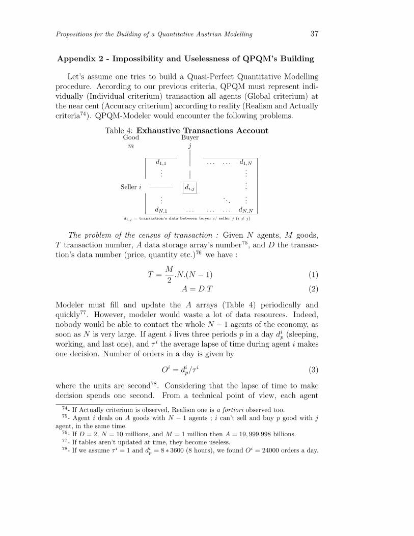
Let’s assume one tries to build a Quasi-Perfect Quantitative Modellingprocedure. According to our previous criteria, QPQM must represent indi-vidually (Individual criterium) transaction all agents (Global criterium) atthe near cent (Accuracy criterium) according to reality (Realism and Actuallycriteria74). QPQM-Modeler would encounter the following problems.

Table 4: Exhaustive Transactions AccountGood Buyerm j

∣

∣

d1,1

∣

∣ . . . . . . d1,N

...∣

∣

...

Seller i ———– di,j

...

.... . .

...dN,1 . . . . . . . . . dN,N

di,j = transaction’s data between buyer i/ seller j (i 6= j)

The problem of the census of transaction : Given N agents, M goods,T transaction number, A data storage array’s number75, and D the transac-tion’s data number (price, quantity etc.)76 we have :

T =M

2.N.(N − 1) (1)

A = D.T (2)

Modeler must fill and update the A arrays (Table 4) periodically andquickly77. However, modeler would waste a lot of data resources. Indeed,nobody would be able to contact the whole N − 1 agents of the economy, assoon as N is very large. If agent i lives three periods p in a day di

p (sleeping,working, and last one), and τ i the average lapse of time during agent i makesone decision. Number of orders in a day is given by

Oi = dip/τ

i (3)

where the units are second78. Considering that the lapse of time to makedecision spends one second. From a technical point of view, each agent

74- If Actually criterium is observed, Realism one is a fortiori observed too.75- Agent i deals on A goods with N − 1 agents ; i can’t sell and buy p good with j

agent, in the same time.76- If D = 2, N = 10 millions, and M = 1 million then A = 19, 999.998 billions.77- If tables aren’t updated at time, they become useless.78- If we assume τ i = 1 and di

p = 8 ∗ 3600 (8 hours), we found Oi = 24000 orders a day.


could indeed program decisions so that order spends one second e.g. on theInternet79.

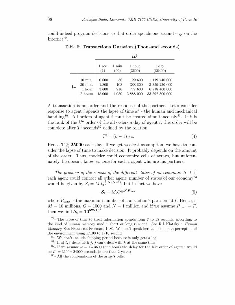
Table 5: Transactions Duration (Thousand seconds)

ω1 sec 1 min 1 hour 1 day(1) (60) (3600) (86400)

τ10 min. 0.600 36 129 600 1 119 740 00030 min. 1.800 108 388 800 3 359 230 0001 hour 3.600 216 777 600 6 718 460 000

5 hours 18.000 1 080 3 888 000 33 592 300 000

A transaction is an order and the response of the partner. Let’s considerresponse to agent i spends the lapse of time ωi - the human and mechanicalhandling80. All orders of agent i can’t be treated simultaneously81. If k isthe rank of the kth order of the all orders a day of agent i, this order will becomplete after T i seconds82 defined by the relation

T i = (k − 1) ∗ ω (4)

Hence T / 25000 each day. If we get weakest assumption, we have to con-sider the lapse of time to make decision. It probably depends on the amountof the order. Thus, modeler could economize cells of arrays, but unfortu-nately, he doesn’t know ex ante for each i agent who are his partners.

The problem of the census of the different states of an economy: At t, ifeach agent could contact all other agent, number of states of our economy83

would be given by St = M.Q1

2.N.(N−1), but in fact we have

St = M.Q1

2.N.Pmax (5)

where Pmax is the maximum number of transaction’s partners at t. Hence, ifM = 10 millions, Q = 1000 and N = 1 million and if we assume Pmax = T ,then we find St = 10

525.109

79- The lapse of time to treat information spends from 7 to 15 seconds, according tothe kind of human memory used : short or long run one. See R.L.Klatzky : HumanMemory, San Francisco, Freeman, 1980. We don’t speak here about human perception ofthe environment using 1/100 to 1/10 second.

80- We don’t include shipping period because it only gets a lag.81- If at t, i deals with j, j can’t deal with k at the same time.82- If we assume ω = 1 ∗ 3600 (one hour) the delay for the last order of agent i would

be Li = 3600 ∗ 24000 seconds (more than 2 years)83- All the combinations of the array’s cells.

Documents

Document de Travail - econ.iastate.edu