Documentation

Brian Kolb and Levi Lentz

PROPhet was written by Brian Kolb and Levi Lentz in the group of Alexie Kolpak at MIT.

Contents

I Introduction 5

II Installation 6

MPI based compile 6

1

Serial compile 6

Linking with the LAMMPS1 MD package 6

Automatic Install . . . . . . . . . . . . . . . . . . . . . . . . . . . . . . . . . . . . 7

Manually linking PROPhet to LAMMPS . . . . . . . . . . . . . . . . . . . . . . . 7

III Quick start / tutorial 8

1 Example : Building a potential (structure → energy) 8

1.1 Introduction . . . . . . . . . . . . . . . . . . . . . . . . . . . . . . . . . . . . 8

1.2 Setting up the PROPhet input file . . . . . . . . . . . . . . . . . . . . . . . . 9

1.3 Training . . . . . . . . . . . . . . . . . . . . . . . . . . . . . . . . . . . . . . 12

1.4 Validate . . . . . . . . . . . . . . . . . . . . . . . . . . . . . . . . . . . . . . 13

1.5 Predict . . . . . . . . . . . . . . . . . . . . . . . . . . . . . . . . . . . . . . . 15

1.6 LAMMPS . . . . . . . . . . . . . . . . . . . . . . . . . . . . . . . . . . . . . 16

1.7 Further information . . . . . . . . . . . . . . . . . . . . . . . . . . . . . . . . 17

IV Reference guide 18

2 command line flags 18

2.1 -train . . . . . . . . . . . . . . . . . . . . . . . . . . . . . . . . . . . . . . . . 18

2.2 -run . . . . . . . . . . . . . . . . . . . . . . . . . . . . . . . . . . . . . . . . 19

2.3 -validate . . . . . . . . . . . . . . . . . . . . . . . . . . . . . . . . . . . . . . 19

3 Specifying data 19

2

Organizing the actual data . . . . . . . . . . . . . . . . . . . . . . . . . . . . . . . 19

Specifying data to PROPhet . . . . . . . . . . . . . . . . . . . . . . . . . . . . . . 20

Per-code caveats . . . . . . . . . . . . . . . . . . . . . . . . . . . . . . . . . . . . 21

The user_input file . . . . . . . . . . . . . . . . . . . . . . . . . . . . . . . . . . . 22

4 The input file 24

4.1 network_type . . . . . . . . . . . . . . . . . . . . . . . . . . . . . . . . . . . 26

4.2 hidden . . . . . . . . . . . . . . . . . . . . . . . . . . . . . . . . . . . . . . 26

4.3 input . . . . . . . . . . . . . . . . . . . . . . . . . . . . . . . . . . . . . . . . 26

4.4 output . . . . . . . . . . . . . . . . . . . . . . . . . . . . . . . . . . . . . . . 27

4.5 transfer . . . . . . . . . . . . . . . . . . . . . . . . . . . . . . . . . . . . . . 27

4.6 algorithm . . . . . . . . . . . . . . . . . . . . . . . . . . . . . . . . . . . . . 27

4.7 threshold . . . . . . . . . . . . . . . . . . . . . . . . . . . . . . . . . . . . . 28

4.8 Niterations . . . . . . . . . . . . . . . . . . . . . . . . . . . . . . . . . . . . 28

4.9 Nprint . . . . . . . . . . . . . . . . . . . . . . . . . . . . . . . . . . . . . . . 28

4.10 Ncheckpoint . . . . . . . . . . . . . . . . . . . . . . . . . . . . . . . . . . . . 28

4.11 checkpoint_in . . . . . . . . . . . . . . . . . . . . . . . . . . . . . . . . . . . 29

4.12 checkpoint_out . . . . . . . . . . . . . . . . . . . . . . . . . . . . . . . . . . 29

4.13 regularization . . . . . . . . . . . . . . . . . . . . . . . . . . . . . . . . . . . 29

4.14 precondition_output . . . . . . . . . . . . . . . . . . . . . . . . . . . . . . . 30

4.15 sd_momentum . . . . . . . . . . . . . . . . . . . . . . . . . . . . . . . . . . 30

4.16 line_min_epsilon . . . . . . . . . . . . . . . . . . . . . . . . . . . . . . . . . 30

4.17 Rcut . . . . . . . . . . . . . . . . . . . . . . . . . . . . . . . . . . . . . . . . 31

4.18 Nradial . . . . . . . . . . . . . . . . . . . . . . . . . . . . . . . . . . . . . . . 31

3

4.19 Nangular . . . . . . . . . . . . . . . . . . . . . . . . . . . . . . . . . . . . . 31

4.20 Mapping function specification . . . . . . . . . . . . . . . . . . . . . . . . . 31

4.20.1 G1 . . . . . . . . . . . . . . . . . . . . . . . . . . . . . . . . . . . . . 32

4.20.2 G2 . . . . . . . . . . . . . . . . . . . . . . . . . . . . . . . . . . . . . 32

4.20.3 G3 . . . . . . . . . . . . . . . . . . . . . . . . . . . . . . . . . . . . . 32

4.20.4 G4 . . . . . . . . . . . . . . . . . . . . . . . . . . . . . . . . . . . . . 33

4.21 data . . . . . . . . . . . . . . . . . . . . . . . . . . . . . . . . . . . . . . . . 33

4.22 include . . . . . . . . . . . . . . . . . . . . . . . . . . . . . . . . . . . . . . . 34

4.23 downsample . . . . . . . . . . . . . . . . . . . . . . . . . . . . . . . . . . . 34

5 Output 35

6 The checkpoint file 35

V Theory 37

7 Charge density 37

8 Structure 38

References 40

4

Part I

Introduction

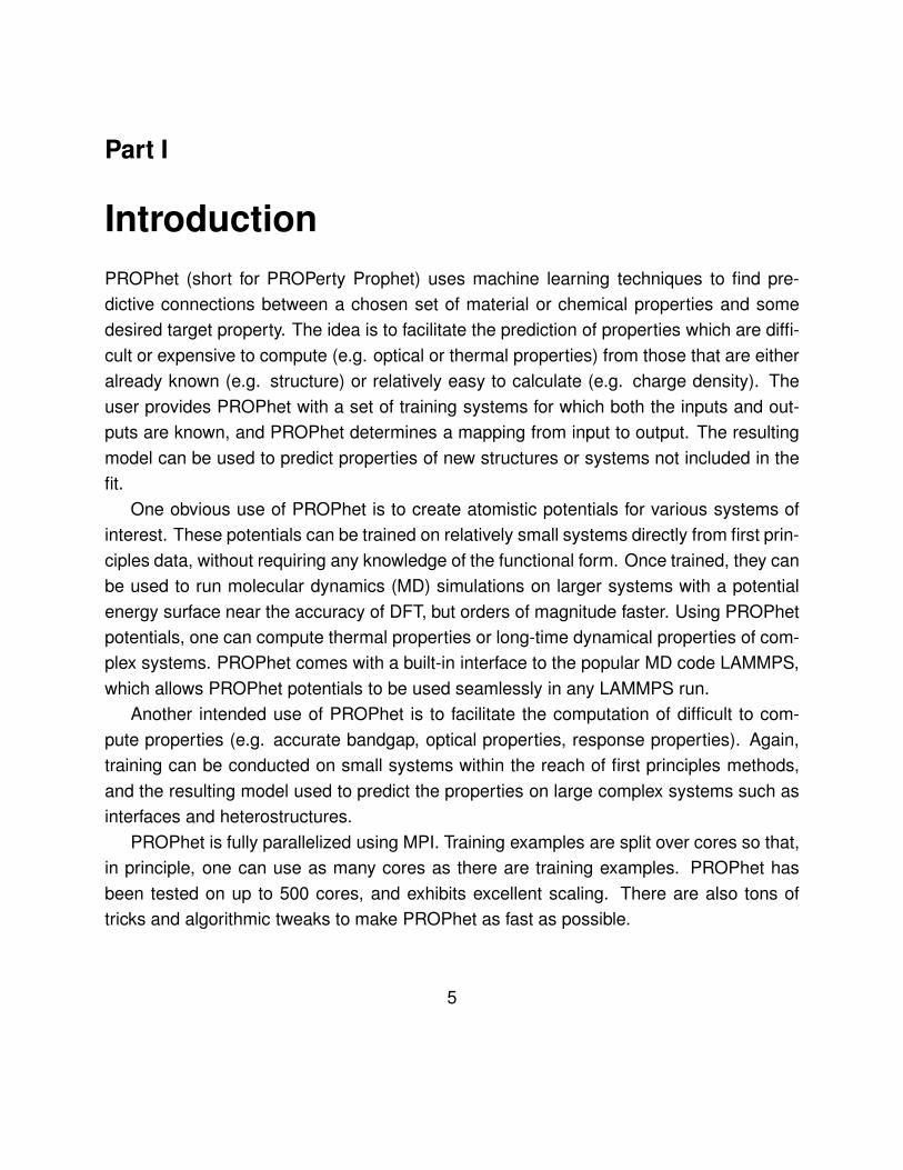
PROPhet (short for PROPerty Prophet) uses machine learning techniques to find pre-

dictive connections between a chosen set of material or chemical properties and some

desired target property. The idea is to facilitate the prediction of properties which are diffi-

cult or expensive to compute (e.g. optical or thermal properties) from those that are either

already known (e.g. structure) or relatively easy to calculate (e.g. charge density). The

user provides PROPhet with a set of training systems for which both the inputs and out-

puts are known, and PROPhet determines a mapping from input to output. The resulting

model can be used to predict properties of new structures or systems not included in the

fit.

One obvious use of PROPhet is to create atomistic potentials for various systems of

interest. These potentials can be trained on relatively small systems directly from first prin-

ciples data, without requiring any knowledge of the functional form. Once trained, they can

be used to run molecular dynamics (MD) simulations on larger systems with a potential

energy surface near the accuracy of DFT, but orders of magnitude faster. Using PROPhet

potentials, one can compute thermal properties or long-time dynamical properties of com-

plex systems. PROPhet comes with a built-in interface to the popular MD code LAMMPS,

which allows PROPhet potentials to be used seamlessly in any LAMMPS run.

Another intended use of PROPhet is to facilitate the computation of difficult to com-

pute properties (e.g. accurate bandgap, optical properties, response properties). Again,

training can be conducted on small systems within the reach of first principles methods,

and the resulting model used to predict the properties on large complex systems such as

interfaces and heterostructures.

PROPhet is fully parallelized using MPI. Training examples are split over cores so that,

in principle, one can use as many cores as there are training examples. PROPhet has

been tested on up to 500 cores, and exhibits excellent scaling. There are also tons of

tricks and algorithmic tweaks to make PROPhet as fast as possible.

5

Part II

Installation

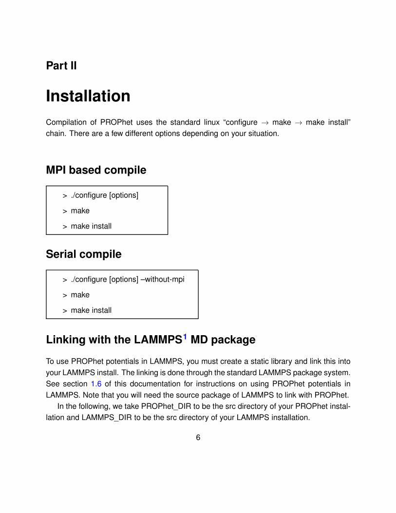
Compilation of PROPhet uses the standard linux “configure → make → make install”

chain. There are a few different options depending on your situation.

MPI based compile

> ./configure [options]

> make

> make install

Serial compile

> ./configure [options] –without-mpi

> make

> make install

Linking with the LAMMPS1 MD package

To use PROPhet potentials in LAMMPS, you must create a static library and link this into

your LAMMPS install. The linking is done through the standard LAMMPS package system.

See section 1.6 of this documentation for instructions on using PROPhet potentials in

LAMMPS. Note that you will need the source package of LAMMPS to link with PROPhet.

In the following, we take PROPhet_DIR to be the src directory of your PROPhet instal-

lation and LAMMPS_DIR to be the src directory of your LAMMPS installation.

6

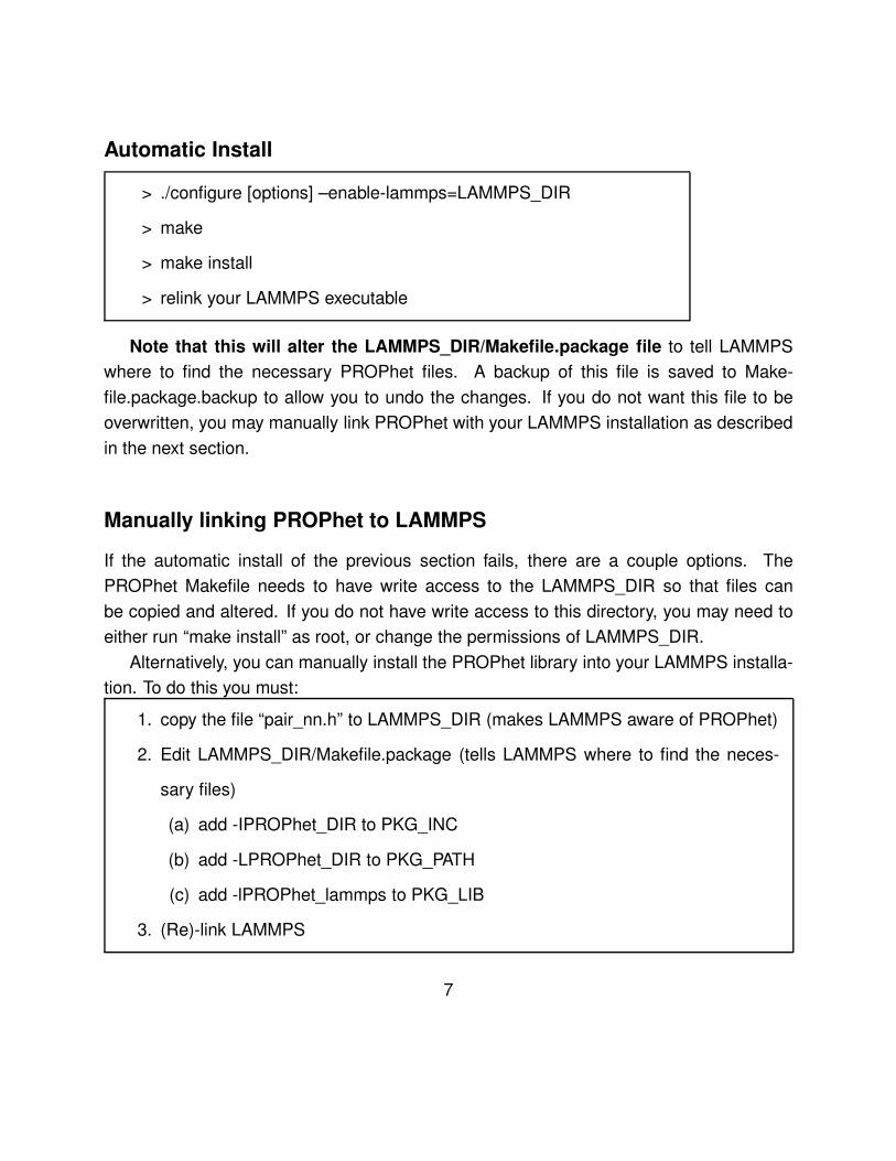
Automatic Install

> ./configure [options] –enable-lammps=LAMMPS_DIR

> make

> make install

> relink your LAMMPS executable

Note that this will alter the LAMMPS_DIR/Makefile.package file to tell LAMMPS

where to find the necessary PROPhet files. A backup of this file is saved to Make-

file.package.backup to allow you to undo the changes. If you do not want this file to be

overwritten, you may manually link PROPhet with your LAMMPS installation as described

in the next section.

Manually linking PROPhet to LAMMPS

If the automatic install of the previous section fails, there are a couple options. The

PROPhet Makefile needs to have write access to the LAMMPS_DIR so that files can

be copied and altered. If you do not have write access to this directory, you may need to

either run “make install” as root, or change the permissions of LAMMPS_DIR.

Alternatively, you can manually install the PROPhet library into your LAMMPS installa-

tion. To do this you must:

1. copy the file “pair_nn.h” to LAMMPS_DIR (makes LAMMPS aware of PROPhet)

2. Edit LAMMPS_DIR/Makefile.package (tells LAMMPS where to find the neces-

sary files)

(a) add -IPROPhet_DIR to PKG_INC

(b) add -LPROPhet_DIR to PKG_PATH

(c) add -lPROPhet_lammps to PKG_LIB

3. (Re)-link LAMMPS

7

Part III

Quick start / tutorial

1 Example : Building a potential (structure → energy)

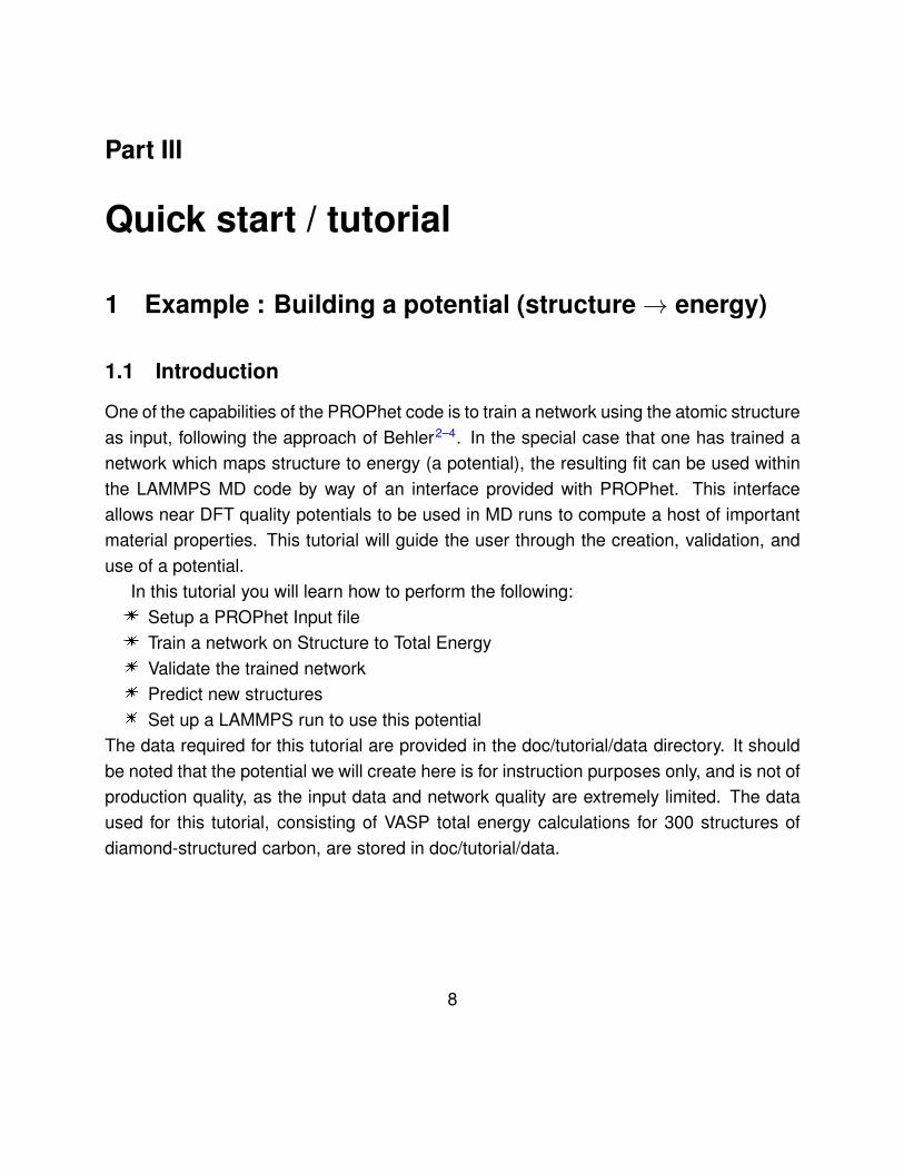
1.1 Introduction

One of the capabilities of the PROPhet code is to train a network using the atomic structure

as input, following the approach of Behler2–4. In the special case that one has trained a

network which maps structure to energy (a potential), the resulting fit can be used within

the LAMMPS MD code by way of an interface provided with PROPhet. This interface

allows near DFT quality potentials to be used in MD runs to compute a host of important

material properties. This tutorial will guide the user through the creation, validation, and

use of a potential.

In this tutorial you will learn how to perform the following:

E Setup a PROPhet Input file

E Train a network on Structure to Total Energy

E Validate the trained network

E Predict new structures

E Set up a LAMMPS run to use this potential

The data required for this tutorial are provided in the doc/tutorial/data directory. It should

be noted that the potential we will create here is for instruction purposes only, and is not of

production quality, as the input data and network quality are extremely limited. The data

used for this tutorial, consisting of VASP total energy calculations for 300 structures of

diamond-structured carbon, are stored in doc/tutorial/data.

8

1.2 Setting up the PROPhet input file

PROPhet uses a single required input file (by default called “input_file”), which holds all

the parameters for the run. PROPhet will expect this file in the directory in which it runs. A

different file name can be specified on the command line with the -in FILE flag. Throughout

this tutorial, we will be using the term input_file as a generic reference to whatever file is

specified for the main input. A fully annotated input_file is supplied with the distribution of

PROPhet (in doc/input_file).

In this tutorial, we will create a potential mapping structure to total energy. Within

the doc/tutorial directory are a number of files, 3 of which are called “input_train”, “in-

put_validate”, and “input_predict”. These are the main PROPhet input files for each stage

of the tutorial. It is generally not necessary to split different phases of the calculations into

different input files, as only minor changes are needed depending on the run. The files

are split here only for convenience.

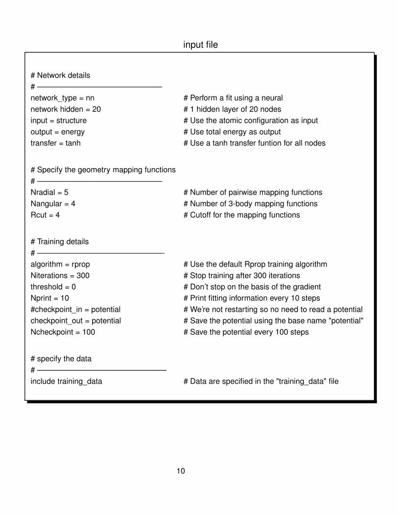
If you examine the input_train file you will find the following:

9

input file

# Network details

# ————————————————

network_type = nn # Perform a fit using a neural

network hidden = 20 # 1 hidden layer of 20 nodes

input = structure # Use the atomic configuration as input

output = energy # Use total energy as output

transfer = tanh # Use a tanh transfer funtion for all nodes

# Specify the geometry mapping functions

# ————————————————

Nradial = 5 # Number of pairwise mapping functions

Nangular = 4 # Number of 3-body mapping functions

Rcut = 4 # Cutoff for the mapping functions

# Training details

# ————————————————-

algorithm = rprop # Use the default Rprop training algorithm

Niterations = 300 # Stop training after 300 iterations

threshold = 0 # Don’t stop on the basis of the gradient

Nprint = 10 # Print fitting information every 10 steps

#checkpoint_in = potential # We’re not restarting so no need to read a potential

checkpoint_out = potential # Save the potential using the base name "potential"

Ncheckpoint = 100 # Save the potential every 100 steps

# specify the data

# ————————————————–

include training_data # Data are specified in the "training_data" file

10

You will notice this input file is broken into four primary areas: "Network Details", "Ge-

ometry Mapping", "Training Details" and "Data Specification". Note that the grouping is

for readability and is not required. With the exception of the “data” statement (described

in data) the input file can be in any order. Also, the input file is case insensitive and

whitespace is ignored.

The Network Details section defines the type of machine learning we will be using.

Currently only neural networks (nn) are implemented. “hidden” specifies the topology of

the network. We are using a single layer of 20 nodes here to make a quick fit. More

layers can be specified with additional integers, each one giving the number of nodes in

that layer (for example, “hidden = 35 35” would give 2 layers, each with 35 nodes). “input”

and “output” define the properties that the network will be trained to, here we are inputting

’structure’ to the network and the output is ’energy.’ Finally, “transfer” is the type of transfer

function in the nodes. We are using hyperbolic tangent functions (tanh).

The Geometry Mapping section defines the key values for generation of the mappings

functions (see Section Mapping function specification and Reference4 for details). In this

case “Nradial” and “Nangular” define 5 and 4 functions, respectively, to be generated

internally by the code. Care must generally be taken here, since, in multi-species systems,

the number of radial and angular functions grows rapidly due to the interaction differences

between the different species. As an example, if we were training CO$_2$ data, Nradial

= 5 would actually generate 10 different 2-body functions per atom in the system. These

would correspond to X-O and X-C interactions (X being the central atom type) for each

of the 5 functions requested. In the case of Nangular = 5, this would swell to 15 as the

X-C-C, X-C-O, and X-O-O interactions have to all be treated separately. Finally, “Rcut” is

the cutoff radius (in \AA) for the mapping functions.

The Training Details section describes how the network is converged. The main point

here to comment on is the “checkpoint_in” and “checkpoint_out” lines. When performing

a training run with PROPhet, the file “checkpoint_out” will be written every “Ncheckpoint”

iterations. This allows for the option to restart the calculation if it gets interrupted before

either “Niterations” or “threshold” are met. If a restart (or a validation, to be describe

later) is desired, un-commenting “checkpoint_in” allows for the network to be reread and

restarted.

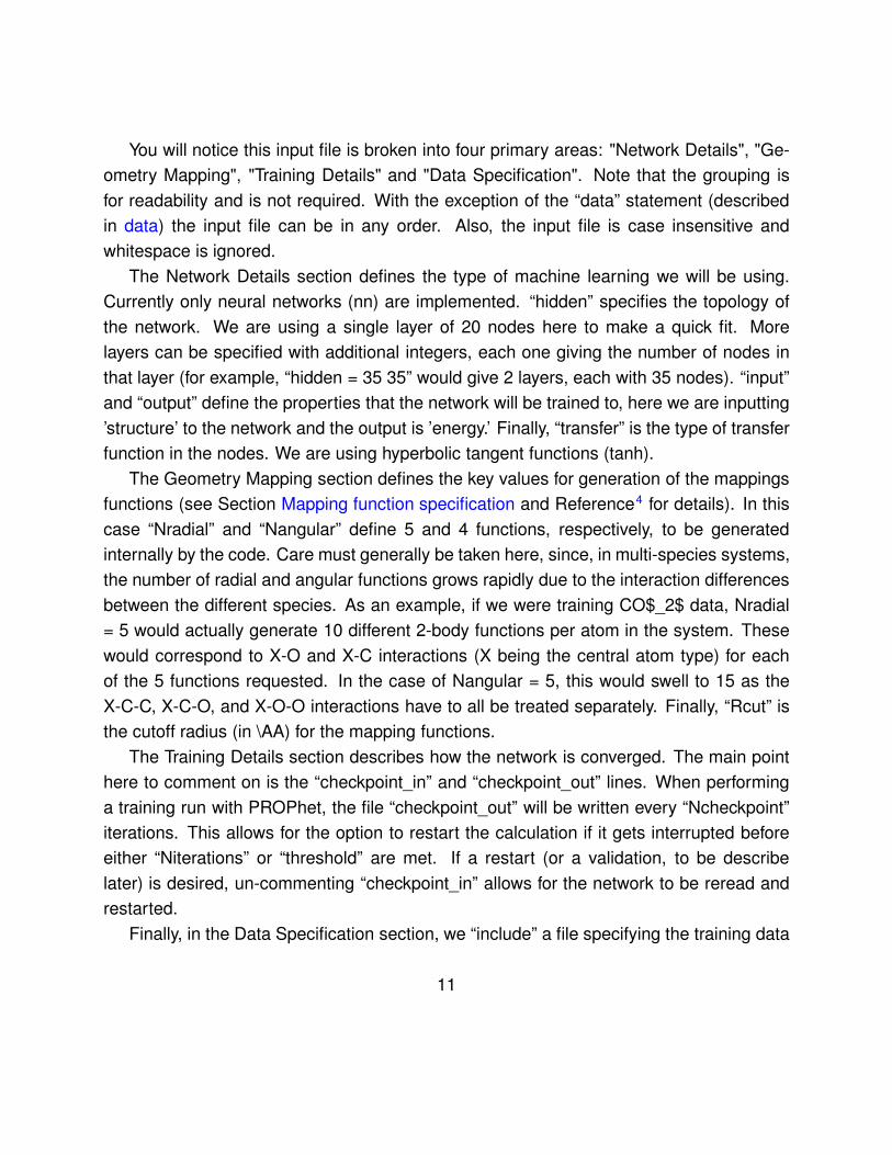
Finally, in the Data Specification section, we “include” a file specifying the training data

11

into the input_file. This is to increase readability as data specification is just a list of

directory locations. While these locations can be specified directly in the input_file, it is

easier to read if you place them in a separate file. The “include” flag in PROPhet works

similarly to the same flag in C/C++, placing the contents of the included file at the spot

where “include” was invoked. For example, this include file training_data looks like the

following:

training_data

data code=vasp

./data/1

./data/2

./data/3

./data/4...

The “code” flag specifies the code that was used to generate the data. Currently VASP,

FHIAims, and Quantum Espresso (QE) can all be specified here. With this information,

PROPhet can read many desired properties directly from the ab initio output files. It is

worth noting that for qe, the energy is not stored in standardized output files. Therefore,

PROPhet cannot read the energy directly from a QE run and this must be specified with

the “user_input” mechanism (see The user_input file).

Now that a basic understanding of the input_file has been described (take a look a the

fully annotated file in the distribution and Section 4 for other options), we are ready to train

the network.

1.3 Training

Examine the input_train and the training_data files. The former contains the parameters

for this training run and the latter contains the data we will use for training. You will notice

that we are only including 250 structures in this training set. The other 50 are set aside

12

to check that the trained potential can predict new structures not included in the training.

This will be performed in the Predict section.

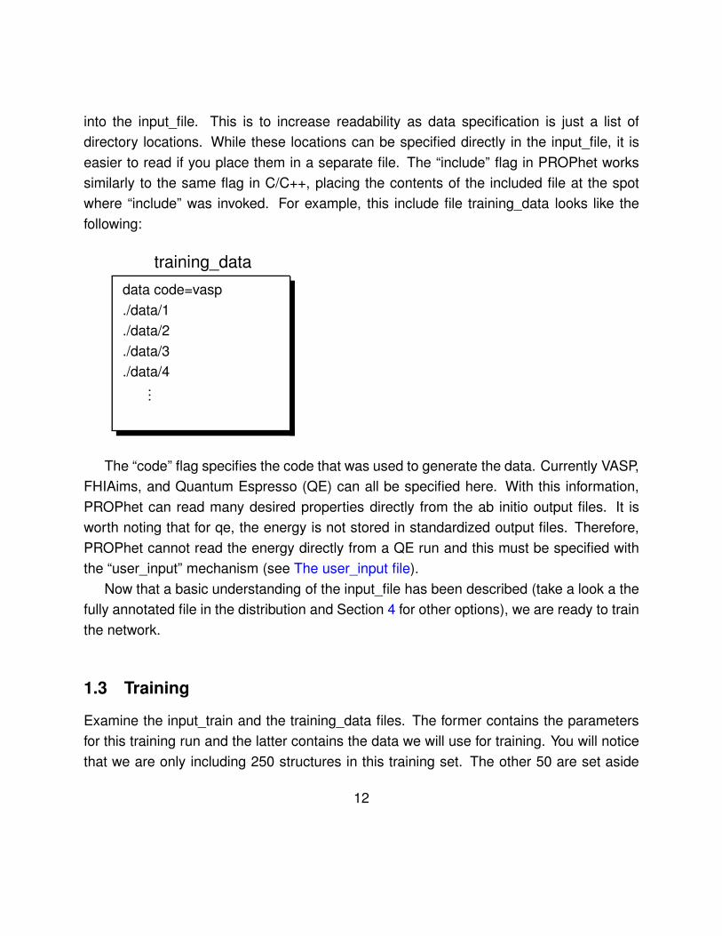
To train the network, you simply specify the “-train” command line flag, as:

> mpirun PROPhet -in input_train -train

Note that “-train” is the default behavior, so the flag can actually be left off.

PROPhet will run for 300 iterations (as is set in the input_file). (Again, note that a

production network will need to be trained with many more data points and iterations.)

The current error of the network is given in the second column of the output. The units of

this quantity are the same as the units of the target values you provided to PROPhet, in

this case, since we are using VASP data, the units are eV. At the completion of the run

you should see a new file called potential_C, which holds the parameters and details of

the current fit. The name of this file is specified in the “checkpoint_out” parameter in the

input_file. Note that the method PROPhet uses to fit structures creates a separate network

for each atomic species present. Thus, the name specified in “checkpoint_out” is the base

name of the files, and PROPhet will automatically append the atomic symbol to this name,

creating a separate file for each atom type and storing the appropriate parameters in each.

Here we have only 1 type, so PROPhet has created only 1 checkpoint file. The checkpoint

file (which is written every Ncheckpoint training steps) is used to restart an interrupted run,

or to use the network for predictions/MD after it has been created. Section 6 discusses

the format of this file.

We now have a PROPhet potential, ready to be tested and used.

1.4 Validate

The first step in making sure that you have a working network is to validate it. A validation

simply ’fires’ the network with a given set of inputs and performs a minimal analysis. This

helps verify that the network is a faithful representation of the data it was trained on.

PROPhet will generate some simple measures of the fidelity of the fit.

Take a look at input_validate and training_data files. The only difference between the

input_train and input_validate files is that the “checkpoint_in” line is un-commented in the

13

latter. When you run with a “-validate” flag PROPhet will read the already trained network

from the file specified in “checkpoint_in” and then ’fire’ it against the data you provide it.

As with the “checkpoint_out” flag, “checkpoint_in” should specify only the base name of

the potential, and PROPhet will automatically handle the atomic species suffixes it added.

To run this manually simply add the “-validate” command line flag as:

> mpirun PROPhet -in input_validate -validate

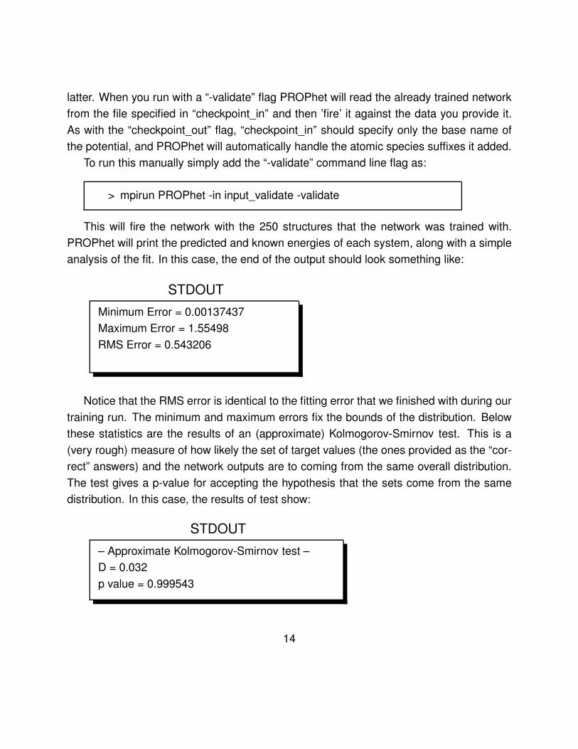
This will fire the network with the 250 structures that the network was trained with.

PROPhet will print the predicted and known energies of each system, along with a simple

analysis of the fit. In this case, the end of the output should look something like:

STDOUT

Minimum Error = 0.00137437

Maximum Error = 1.55498

RMS Error = 0.543206

Notice that the RMS error is identical to the fitting error that we finished with during our

training run. The minimum and maximum errors fix the bounds of the distribution. Below

these statistics are the results of an (approximate) Kolmogorov-Smirnov test. This is a

(very rough) measure of how likely the set of target values (the ones provided as the “cor-

rect” answers) and the network outputs are to coming from the same overall distribution.

The test gives a p-value for accepting the hypothesis that the sets come from the same

distribution. In this case, the results of test show:

STDOUT

– Approximate Kolmogorov-Smirnov test –

D = 0.032

p value = 0.999543

14

This test is meant only as a guide to compare different fits, and the results should

not be taken to be quantitative measures of fitness.

1.5 Predict

The power of PROPhet is the ability to predict properties of interest for systems that were

not used in fitting. By setting aside the 50 structures in the beginning of the training, we

can now test the network on those 50 structures. In other words, we want to ’fire’ the

network while feeding in these unknown structures.

Take a look at input_predict and training_data. You will notice that input_predict is iden-

tical to that in the validation example except for the data included. In “predict_data” you

will only find 50 data points, none of which were included in the fit. To test the predictive

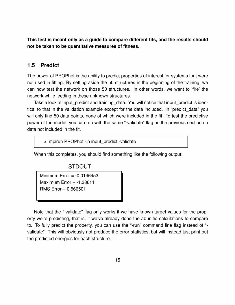
power of the model, you can run with the same “-validate” flag as the previous section on

data not included in the fit.

> mpirun PROPhet -in input_predict -validate

When this completes, you should find something like the following output:

STDOUT

Minimum Error = -0.0146453

Maximum Error = -1.38611

RMS Error = 0.566501

Note that the “-validate” flag only works if we have known target values for the prop-

erty we’re predicting, that is, if we’ve already done the ab initio calculations to compare

to. To fully predict the property, you can use the “-run” command line flag instead of “-

validate”. This will obviously not produce the error statistics, but will instead just print out

the predicted energies for each structure.

15

1.6 LAMMPS

Once you have a potential, you probably want to do something with it. PROPhet includes

an interface to the popular MD code LAMMPS5, so you can use PROPhet potentials in

sophisticated MD runs. Using PROPhet potentials within LAMMPS is fairly straightforward.

(Note that you will need to use a LAMMPS executable that has had PROPhet linked in.

This process is described in section II. If you run the following without a properly compiled

LAMMPS executable, the code will simply die at the potential setting step.) The key lines

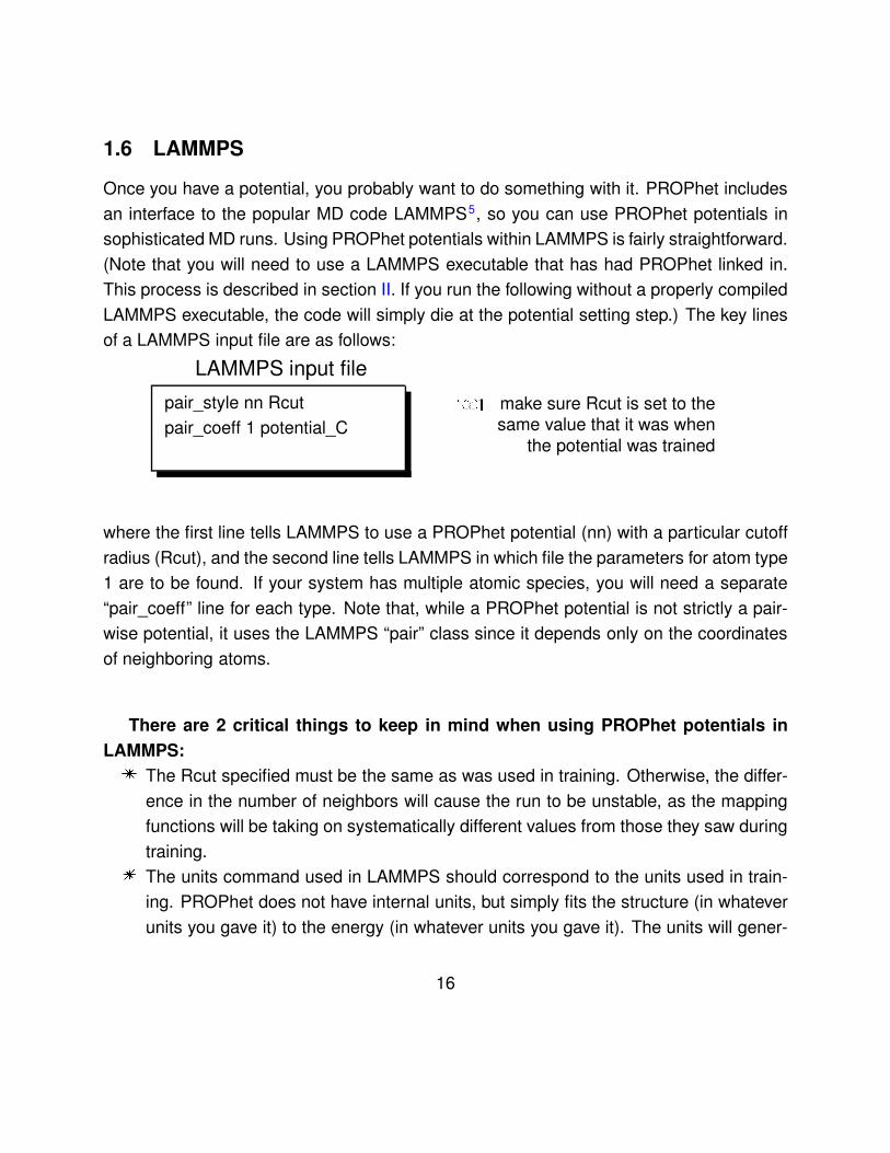
of a LAMMPS input file are as follows:

LAMMPS input file

pair_style nn Rcut

pair_coeff 1 potential_C

L make sure Rcut is set to thesame value that it was when

the potential was trained

where the first line tells LAMMPS to use a PROPhet potential (nn) with a particular cutoff

radius (Rcut), and the second line tells LAMMPS in which file the parameters for atom type

1 are to be found. If your system has multiple atomic species, you will need a separate

“pair_coeff” line for each type. Note that, while a PROPhet potential is not strictly a pair-

wise potential, it uses the LAMMPS “pair” class since it depends only on the coordinates

of neighboring atoms.

There are 2 critical things to keep in mind when using PROPhet potentials in

LAMMPS:

E The Rcut specified must be the same as was used in training. Otherwise, the differ-

ence in the number of neighbors will cause the run to be unstable, as the mapping

functions will be taking on systematically different values from those they saw during

training.

E The units command used in LAMMPS should correspond to the units used in train-

ing. PROPhet does not have internal units, but simply fits the structure (in whatever

units you gave it) to the energy (in whatever units you gave it). The units will gener-

16

ally depend on which code generated the data, unless units were converted explicitly

before training.

1.7 Further information

This is the basic flow of using PROPhet to fit system properties. This tutorial has given

an example of fitting atomic structure to the total energy, but there are many other proper-

ties that PROPhet can extract automatically from data files (see section 4.3 for a list). In

addition, since the property of interest may not be in this list, PROPhet provides a mecha-

nism by which the user can provide their own property data. This mechanism is discussed

in section 3. Note that, because of a complication in the way Quantum Espresso stores

information in its files, PROPhet cannot automatically extract the total energy from a QE

run. If you want to use the energy from a QE run in a PROPhet fit, you must use this

mechanism.

17

Part IV

Reference guide

This section is intended to be a reference for the input and command line parameters

needed to run PROPhet effectively.

2 command line flags

Most control parameters should be specified in the input file. Command line flags are used

to tell PROPhet where to find the input file, and what to do with what it finds there. For

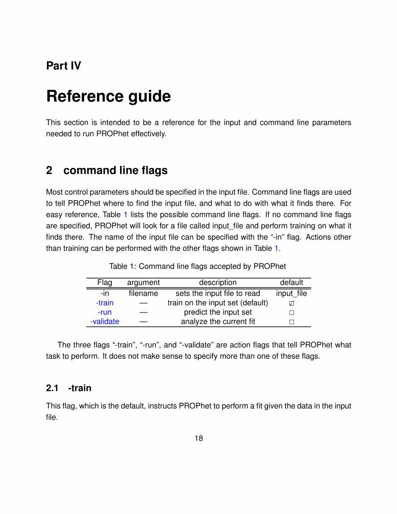
easy reference, Table 1 lists the possible command line flags. If no command line flags

are specified, PROPhet will look for a file called input_file and perform training on what it

finds there. The name of the input file can be specified with the “-in” flag. Actions other

than training can be performed with the other flags shown in Table 1.

Table 1: Command line flags accepted by PROPhet

Flag argument description default

-in filename sets the input file to read input_file-train — train on the input set (default) 2

-run — predict the input set 2

-validate — analyze the current fit 2

The three flags “-train”, “-run”, and “-validate” are action flags that tell PROPhet what

task to perform. It does not make sense to specify more than one of these flags.

2.1 -train

This flag, which is the default, instructs PROPhet to perform a fit given the data in the input

file.

18

2.2 -run

This flag instructs PROPhet to perform predictions on the data using a pre-existing fit.

Note that that “checkpoint_in”, which specifies the existing network, must be specified in

the input file (see Section 4).

2.3 -validate

This flag tells PROPhet to perform some analysis of a pre-existing fit. Generally, this

should be done with the fitting data after the fit has been performed. PROPhet will print

out all the network outputs and their associated targets, as well as some statistics re-

garding the fit. Included is an approximate Kolmogorov-Smirnov statistic, which indicates

the likelihood that two distributions are the same. In this case, the two distributions are

the set of network outputs and the set of targets. If these are deemed significantly differ-

ent, it is likely the fit needs to be improved. This statistic is advantageous as it makes no

assumptions about the form of the distributions, and is robust to shape and scale changes.

3 Specifying data

The most important part of using PROPhet is specifying the data set for training or predic-

tions (we will call these the training examples). For many properties, PROPhet can extract

the data automatically from the output files of several codes (currently VASP, Quantum

Espresso, and FHI-aims). For VASP and Quantum Espresso, the data are extracted from

the xml files they write, while the data are pulled from a plain text output file for FHI-Aims.

Organizing the actual data

There should be a separate base directory for each different training example (generally a

training example will correspond to a particular structure). If multiple properties are being

used as inputs/output, they can come from a single run or several different runs. If the

19

runs are separate, the data for each property should be stored in subdirectories of the

base directory for that training example. These can be named as desired, we will tell

PROPhet how to find the data next.

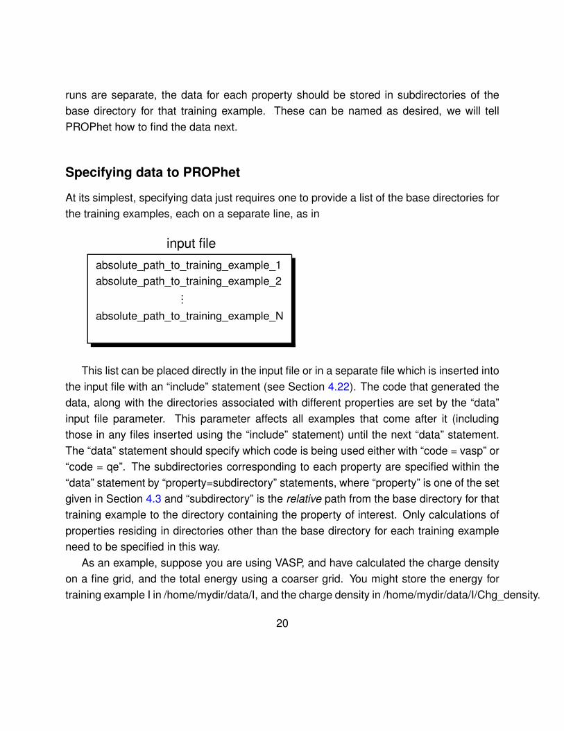
Specifying data to PROPhet

At its simplest, specifying data just requires one to provide a list of the base directories for

the training examples, each on a separate line, as in

input file

absolute_path_to_training_example_1

absolute_path_to_training_example_2...

absolute_path_to_training_example_N

This list can be placed directly in the input file or in a separate file which is inserted into

the input file with an “include” statement (see Section 4.22). The code that generated the

data, along with the directories associated with different properties are set by the “data”

input file parameter. This parameter affects all examples that come after it (including

those in any files inserted using the “include” statement) until the next “data” statement.

The “data” statement should specify which code is being used either with “code = vasp” or

“code = qe”. The subdirectories corresponding to each property are specified within the

“data” statement by “property=subdirectory” statements, where “property” is one of the set

given in Section 4.3 and “subdirectory” is the relative path from the base directory for that

training example to the directory containing the property of interest. Only calculations of

properties residing in directories other than the base directory for each training example

need to be specified in this way.

As an example, suppose you are using VASP, and have calculated the charge density

on a fine grid, and the total energy using a coarser grid. You might store the energy for

training example I in /home/mydir/data/I, and the charge density in /home/mydir/data/I/Chg_density.

20

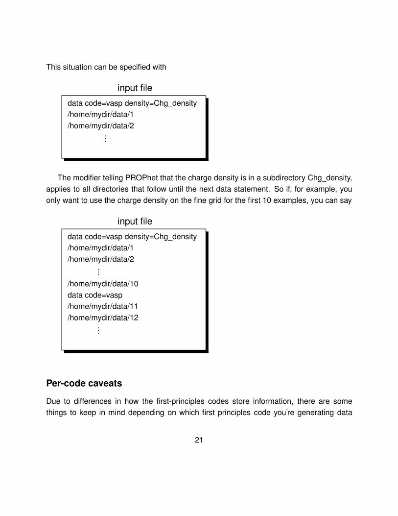
This situation can be specified with

input file

data code=vasp density=Chg_density

/home/mydir/data/1

/home/mydir/data/2...

The modifier telling PROPhet that the charge density is in a subdirectory Chg_density,

applies to all directories that follow until the next data statement. So if, for example, you

only want to use the charge density on the fine grid for the first 10 examples, you can say

input file

data code=vasp density=Chg_density

/home/mydir/data/1

/home/mydir/data/2...

/home/mydir/data/10

data code=vasp

/home/mydir/data/11

/home/mydir/data/12...

Per-code caveats

Due to differences in how the first-principles codes store information, there are some

things to keep in mind depending on which first principles code you’re generating data

21

with.

VASP VASP writes an xml file (vasprun.xml) to the directory in which the run is conducted,

so this is the directory that should be given to PROPhet.

QE Quantum Espresso creates a subdirectory (by default called pwscf.save) in which it

stores the xml and charge density files. This subdirectory should be used as the

base directory for specifying QE data to PROPhet. Also, the total energy is not

written to the QE xml file. If you want to use energy computed with QE with a

network you must either use the user_input file (see Section 3) or put the energy into

the xml file yourself by adding the line <TOTAL_ENERGY> put_QE_energy_here

</TOTAL_ENERGY> to the xml file of each training example.

FHI-Aims FHI-Aims does not write standard files during runtime. Instead, it prints its data

to STDOUT, which must be redirected to a file. Rather than require the user to name

this file a certain ways, PROPhet requires that the name of the file instead of the

directory in which it resides as is the case for VASP and QE data.

The user_input file

It is possible to use PROPhet with properties not handled by the built-in interface. These

can be given to PROPhet via a special file called “user_input”. Lines in this file correspond

to values you want PROPhet to use for training. Each line corresponds to a single property,

which can be either a scalar or a vector. As with built-in properties, these user-defined

properties are given to PROPhet in “input” and “output” statements in the input file using

the parameter

user#

where # is an integer giving the line number of that property (starting from 1) in the

user_input file.

For example, suppose you wanted a network to fit the 9 elements of the dielectric

tensor and the total energy to the fermi level, you could do this by specifying

22

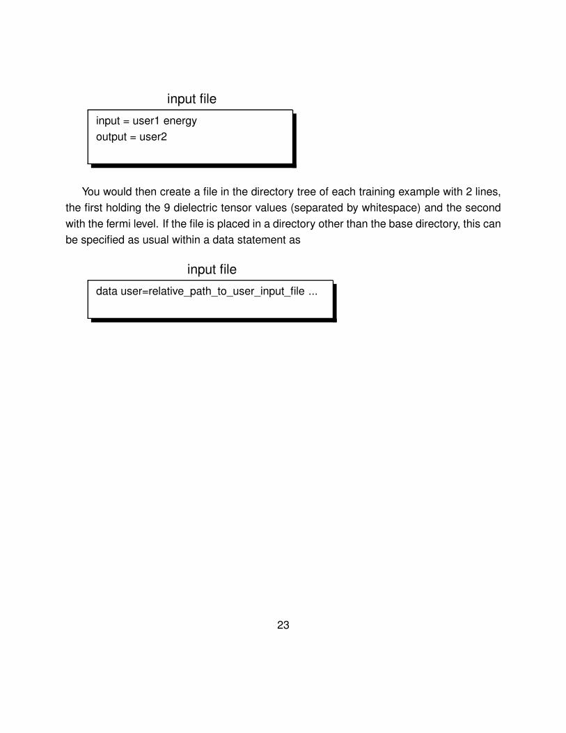
input file

input = user1 energy

output = user2

You would then create a file in the directory tree of each training example with 2 lines,

the first holding the 9 dielectric tensor values (separated by whitespace) and the second

with the fermi level. If the file is placed in a directory other than the base directory, this can

be specified as usual within a data statement as

input file

data user=relative_path_to_user_input_file ...

23

4 The input file

The input file of PROPhet is free format; whitespace is ignored and the file is not case

sensitive (with the exception of directory/file names). Comments can be started with the

“#” character. Parameters are specified by parameter=value pairs, and can be given in

any order, with the exception of data blocks (see section 4.21).

24

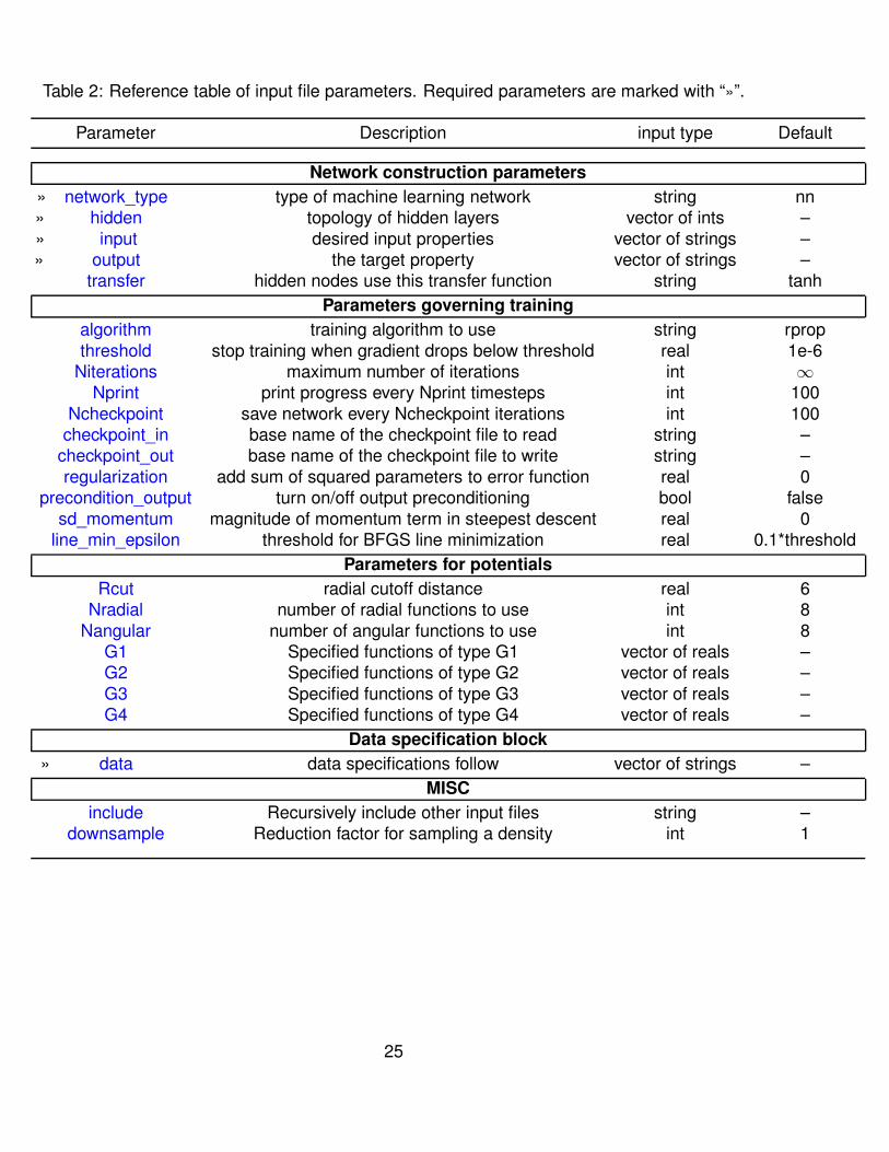
Table 2: Reference table of input file parameters. Required parameters are marked with “»”.

Parameter Description input type Default

Network construction parameters

» network_type type of machine learning network string nn» hidden topology of hidden layers vector of ints –» input desired input properties vector of strings –» output the target property vector of strings –

transfer hidden nodes use this transfer function string tanh

Parameters governing training

algorithm training algorithm to use string rpropthreshold stop training when gradient drops below threshold real 1e-6

Niterations maximum number of iterations int ∞

Nprint print progress every Nprint timesteps int 100Ncheckpoint save network every Ncheckpoint iterations int 100

checkpoint_in base name of the checkpoint file to read string –checkpoint_out base name of the checkpoint file to write string –regularization add sum of squared parameters to error function real 0

precondition_output turn on/off output preconditioning bool falsesd_momentum magnitude of momentum term in steepest descent real 0

line_min_epsilon threshold for BFGS line minimization real 0.1*threshold

Parameters for potentials

Rcut radial cutoff distance real 6Nradial number of radial functions to use int 8

Nangular number of angular functions to use int 8G1 Specified functions of type G1 vector of reals –G2 Specified functions of type G2 vector of reals –G3 Specified functions of type G3 vector of reals –G4 Specified functions of type G4 vector of reals –

Data specification block

» data data specifications follow vector of strings –

MISC

include Recursively include other input files string –downsample Reduction factor for sampling a density int 1

25

4.1 network_type

value string

description This determines the underlying machine learning method to use. Currently

only neural_networks (nn) are implemented.

4.2 hidden

value vector of ints

description This determines the network topology by specifying the hidden nodes. There

should be 1 integer for each layer, specifying the number of nodes in that layer. For

example, a network with 2 hidden layers of 10 and 15 nodes would be specified by

“hidden = 10 15”. Note that input and output layers are not specified here, but are

determined automatically by PROPhet.

4.3 input

value vector of strings

description These are the system properties to use as input to the network. The current

built-in possibilities are

Eenergy Edensity Eenergy

Evolume Edft_gap Egw_gap

Euser# (see The user_input file)

PROPhet will automatically extract these properties from the output files of their runs.

With the exception of “structure”, which can currently only be used alone, any combination

of these properties can be specified for input.

26

4.4 output

value string

description Same as input, except that currently only a single output can be specified.

Also, it is not possible to use “structure” as an output.

4.5 transfer

value string

description The non-linear transfer function to be used by hidden nodes (the output node

is always linear). Current options are

E tanh

E tanh_spline

Specifying the transfer function in the input file sets all hidden nodes with this function.

The transfer function can be set on a per-node basis by editing the checkpoint file (see

Section 6)

4.6 algorithm

value string

description This sets the training algorithm to use. Current options are

E rprop

E steepest_descent

E bfgs

Rprop (which is the default) specifies a flavor of the resilient backpropagation algorithm

and is an excellent choice in the initial stages of training when one starts far from the

minimum.

Steepest descent is steepest descent with an adaptive step size. One can couple this

with the “sd_momentum” parameter to use a momentum term that includes a portion (set

by the magnitude of sd_momentum) of the previous step into the current step.

BFGS invokes the limited memory BFGS algorithm, and is a good choice when close

to the minimum. This option performs a line minimization using Brent’s method at each

27

step. Because of this, care should be taken that one has reached a convex and relatively

smooth region of parameter space (i.e. generally don’t use this in the initial stages of

training). Also, the line minimization can require many sub-steps, so each step can take

significantly longer than either Rprop or steepest_descent, but more progress should be

made on each step.

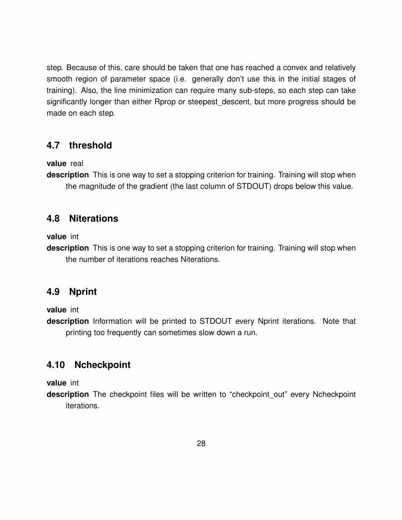
4.7 threshold

value real

description This is one way to set a stopping criterion for training. Training will stop when

the magnitude of the gradient (the last column of STDOUT) drops below this value.

4.8 Niterations

value int

description This is one way to set a stopping criterion for training. Training will stop when

the number of iterations reaches Niterations.

4.9 Nprint

value int

description Information will be printed to STDOUT every Nprint iterations. Note that

printing too frequently can sometimes slow down a run.

4.10 Ncheckpoint

value int

description The checkpoint files will be written to “checkpoint_out” every Ncheckpoint

iterations.

28

4.11 checkpoint_in

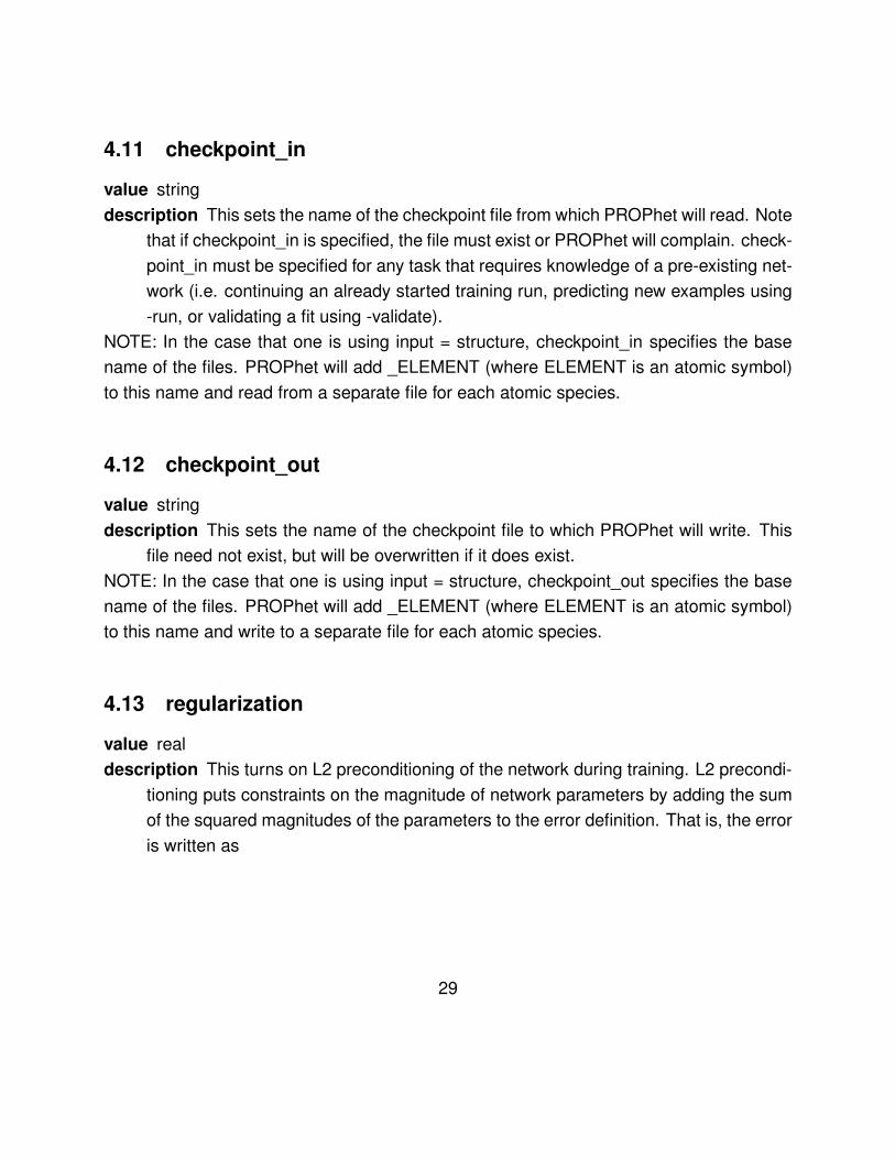
value string

description This sets the name of the checkpoint file from which PROPhet will read. Note

that if checkpoint_in is specified, the file must exist or PROPhet will complain. check-

point_in must be specified for any task that requires knowledge of a pre-existing net-

work (i.e. continuing an already started training run, predicting new examples using

-run, or validating a fit using -validate).

NOTE: In the case that one is using input = structure, checkpoint_in specifies the base

name of the files. PROPhet will add _ELEMENT (where ELEMENT is an atomic symbol)

to this name and read from a separate file for each atomic species.

4.12 checkpoint_out

value string

description This sets the name of the checkpoint file to which PROPhet will write. This

file need not exist, but will be overwritten if it does exist.

NOTE: In the case that one is using input = structure, checkpoint_out specifies the base

name of the files. PROPhet will add _ELEMENT (where ELEMENT is an atomic symbol)

to this name and write to a separate file for each atomic species.

4.13 regularization

value real

description This turns on L2 preconditioning of the network during training. L2 precondi-

tioning puts constraints on the magnitude of network parameters by adding the sum

of the squared magnitudes of the parameters to the error definition. That is, the error

is written as

29

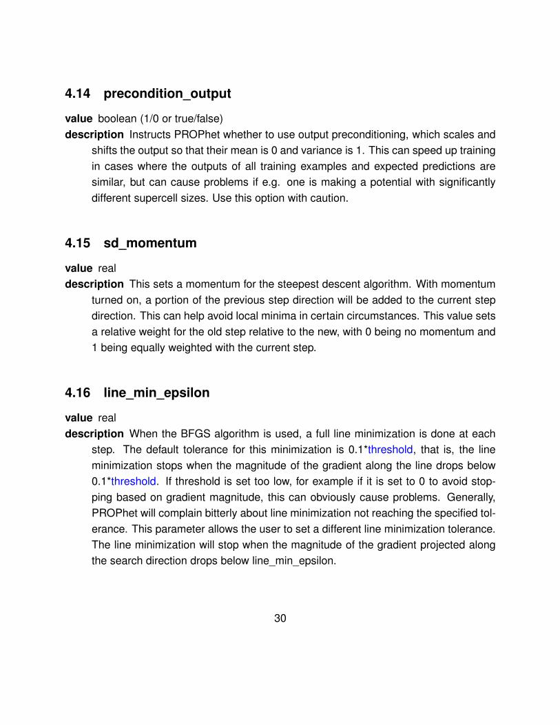
4.14 precondition_output

value boolean (1/0 or true/false)

description Instructs PROPhet whether to use output preconditioning, which scales and

shifts the output so that their mean is 0 and variance is 1. This can speed up training

in cases where the outputs of all training examples and expected predictions are

similar, but can cause problems if e.g. one is making a potential with significantly

different supercell sizes. Use this option with caution.

4.15 sd_momentum

value real

description This sets a momentum for the steepest descent algorithm. With momentum

turned on, a portion of the previous step direction will be added to the current step

direction. This can help avoid local minima in certain circumstances. This value sets

a relative weight for the old step relative to the new, with 0 being no momentum and

1 being equally weighted with the current step.

4.16 line_min_epsilon

value real

description When the BFGS algorithm is used, a full line minimization is done at each

step. The default tolerance for this minimization is 0.1*threshold, that is, the line

minimization stops when the magnitude of the gradient along the line drops below

0.1*threshold. If threshold is set too low, for example if it is set to 0 to avoid stop-

ping based on gradient magnitude, this can obviously cause problems. Generally,

PROPhet will complain bitterly about line minimization not reaching the specified tol-

erance. This parameter allows the user to set a different line minimization tolerance.

The line minimization will stop when the magnitude of the gradient projected along

the search direction drops below line_min_epsilon.

30

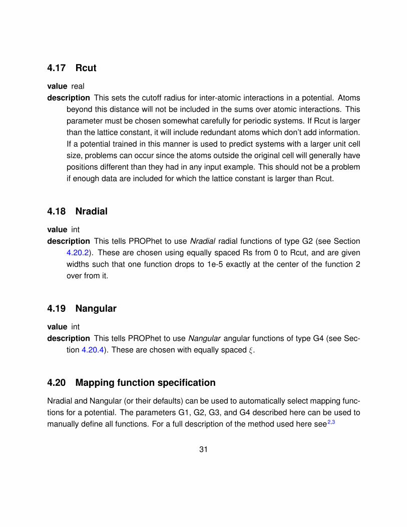
4.17 Rcut

value real

description This sets the cutoff radius for inter-atomic interactions in a potential. Atoms

beyond this distance will not be included in the sums over atomic interactions. This

parameter must be chosen somewhat carefully for periodic systems. If Rcut is larger

than the lattice constant, it will include redundant atoms which don’t add information.

If a potential trained in this manner is used to predict systems with a larger unit cell

size, problems can occur since the atoms outside the original cell will generally have

positions different than they had in any input example. This should not be a problem

if enough data are included for which the lattice constant is larger than Rcut.

4.18 Nradial

value int

description This tells PROPhet to use Nradial radial functions of type G2 (see Section

4.20.2). These are chosen using equally spaced Rs from 0 to Rcut, and are given

widths such that one function drops to 1e-5 exactly at the center of the function 2

over from it.

4.19 Nangular

value int

description This tells PROPhet to use Nangular angular functions of type G4 (see Sec-

tion 4.20.4). These are chosen with equally spaced ξ.

4.20 Mapping function specification

Nradial and Nangular (or their defaults) can be used to automatically select mapping func-

tions for a potential. The parameters G1, G2, G3, and G4 described here can be used to

manually define all functions. For a full description of the method used here see2,3

31

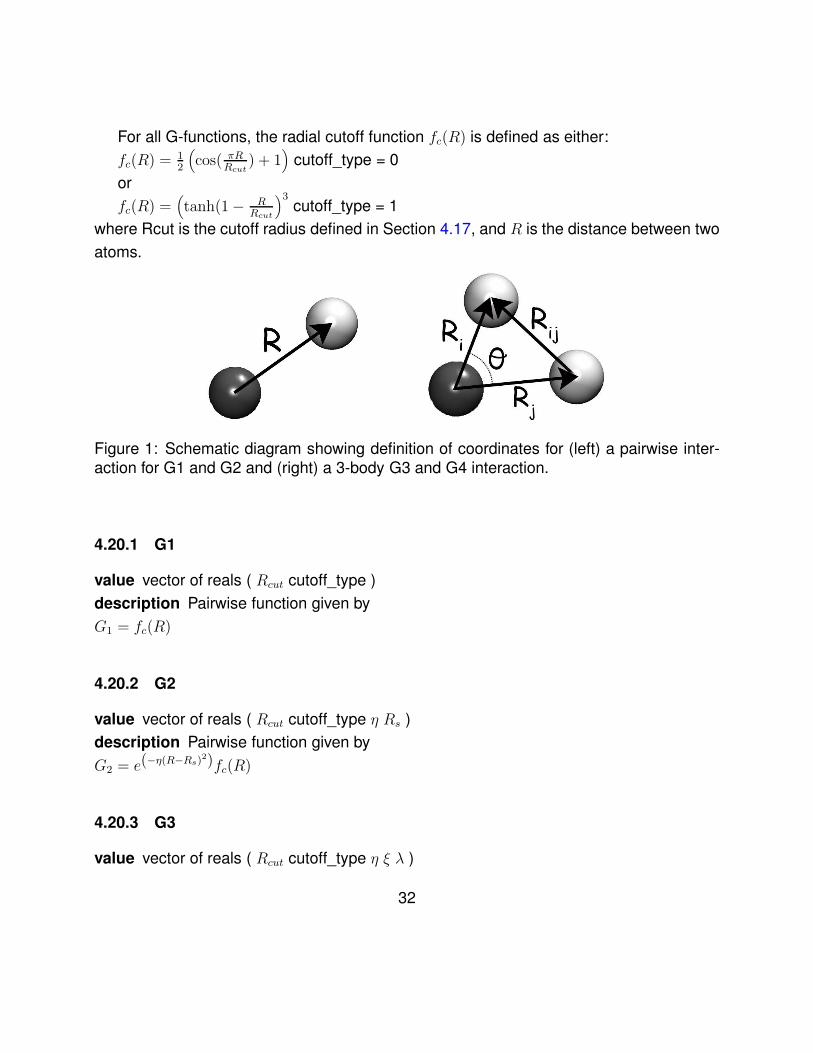
For all G-functions, the radial cutoff function fc(R) is defined as either:

fc(R) = 12

(

cos( πRRcut

) + 1)

cutoff_type = 0

or

fc(R) =(

tanh(1− RRcut

)3cutoff_type = 1

where Rcut is the cutoff radius defined in Section 4.17, and R is the distance between two

atoms.

Figure 1: Schematic diagram showing definition of coordinates for (left) a pairwise inter-action for G1 and G2 and (right) a 3-body G3 and G4 interaction.

4.20.1 G1

value vector of reals ( Rcut cutoff_type )

description Pairwise function given by

G1 = fc(R)

4.20.2 G2

value vector of reals ( Rcut cutoff_type η Rs )

description Pairwise function given by

G2 = e(−η(R−Rs)2)fc(R)

4.20.3 G3

value vector of reals ( Rcut cutoff_type η ξ λ )

32

description 3-body function given by

G3 = 2(1−ξ) (1 + λ cos(θ))ξ e(−η(R2

i+R2

j+R2

ij))fc(Ri)fc(Rj)fc(Rij)

(see Figure ?? for coordinate definitions).

4.20.4 G4

value vector of reals (Rcut cutoff_type η ξ λ )

description 3-body function given by

G4 = 2(1−ξ) (1 + λ cos(θ)) e(−(R2

i+R2

j))fc(Ri)fc(Rj)

(see Figure ?? for coordinate definitions)

4.21 data

value vector of strings (format parameter=value)

description While data in PROPhet are specified as a series of input lines containing

base directory/file names, this critical parameter modifies how these data are han-

dled. The modification affects all input lines that follow until the next data statement.

The most important parameter here is “code” which tells PROPhet which code (cur-

rently VASP, QE, or FHIAims) was used to generate the data. PROPhet will extract

the necessary properties directly from the output files. Note that any code can be

used with PROPhet if the data can be massaged into the format of one of these

codes. The remaining parameters modify the directory (relative to the base) for each

property specified in “input”. This feature allows different properties to be computed

in separate runs. For example, to do a network fitting the DFT band gap (computed

in the base directory) to the band gap computed with the GW method (computed in

a subdirectory called GW), both computed in VASP, the data line should read “data

code=vasp gw_gap=GW”. Note that if all properties are to be taken from a single

run, only the “code” parameter needs to be specified.

33

4.22 include

value string (filename)

description This powerful parameter allows the user to recursively insert input files. The

include parameter in PROPhet works similarly to the way it works in the C/C++ lan-

guage. The file named in “value” is essentially pasted to this location in the input

file. This command can be stacked, i.e. a file included can itself contain include

directives. This parameter can be used to easily switch data sets for training and

testing. The different sets can be specified in different files which are selected with

the appropriate “include” statement. It can also be used to switch training schemes

for the same data set.

4.23 downsample

value int

description When providing a charge density to PROPhet, it is sometimes useful to

speed calculations by sampling the density on a coarser grid than the one pro-

vided. Setting “downsample” resamples the density by averaging over blocks of

size N ×N ×N . Note that it is currently only possible to use this flag with densities

from VASP, and the blocks must be cubic (i.e. you can’t specify different step sizes

per direction).

34

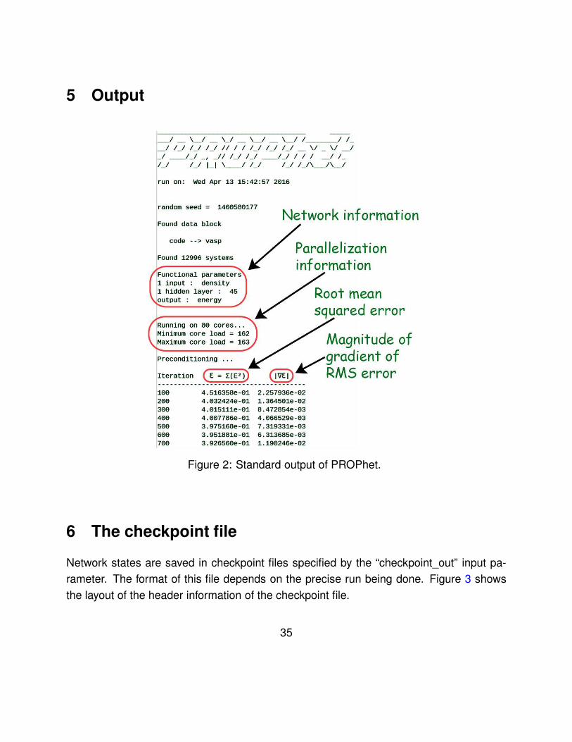
5 Output

Figure 2: Standard output of PROPhet.

6 The checkpoint file

Network states are saved in checkpoint files specified by the “checkpoint_out” input pa-

rameter. The format of this file depends on the precise run being done. Figure 3 shows

the layout of the header information of the checkpoint file.

35

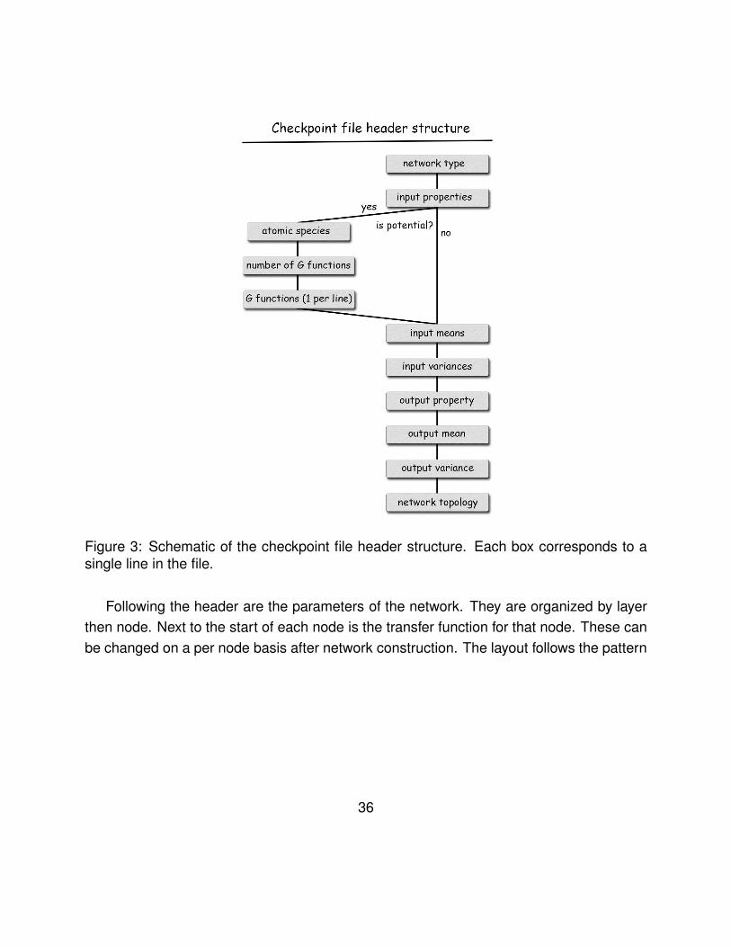
Figure 3: Schematic of the checkpoint file header structure. Each box corresponds to asingle line in the file.

Following the header are the parameters of the network. They are organized by layer

then node. Next to the start of each node is the transfer function for that node. These can

be changed on a per node basis after network construction. The layout follows the pattern

36

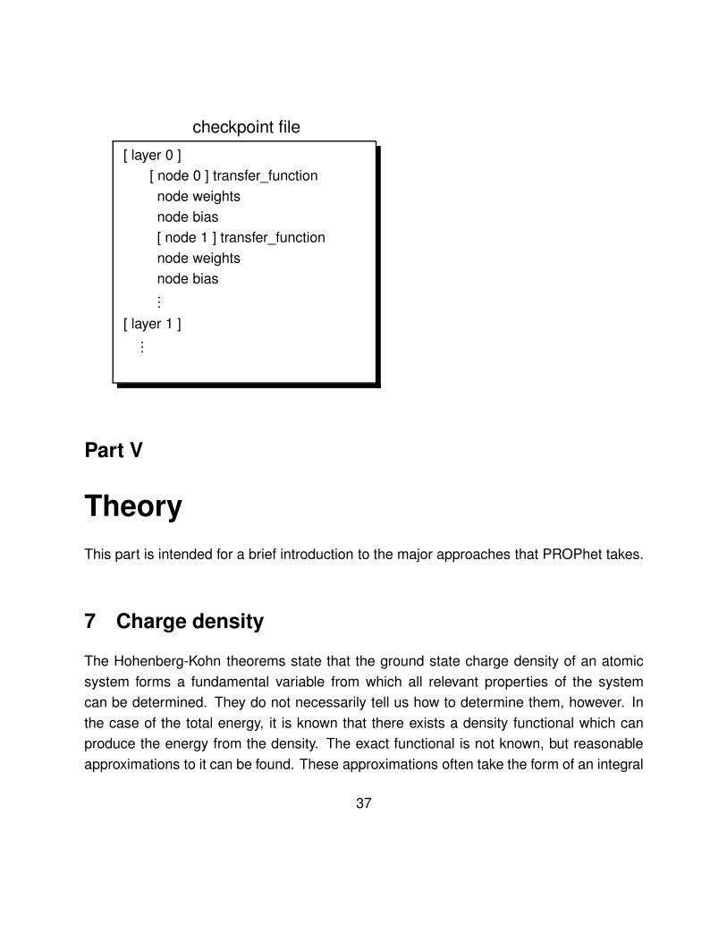
checkpoint file

[ layer 0 ]

[ node 0 ] transfer_function

node weights

node bias

[ node 1 ] transfer_function

node weights

node bias...

[ layer 1 ]...

Part V

Theory

This part is intended for a brief introduction to the major approaches that PROPhet takes.

7 Charge density

The Hohenberg-Kohn theorems state that the ground state charge density of an atomic

system forms a fundamental variable from which all relevant properties of the system

can be determined. They do not necessarily tell us how to determine them, however. In

the case of the total energy, it is known that there exists a density functional which can

produce the energy from the density. The exact functional is not known, but reasonable

approximations to it can be found. These approximations often take the form of an integral

37

over some function of the charge density (LDA) or the density and its gradient (GGA).

In principle procedure could hold for approximations of properties besides energy, except

that there is no intuitive form for the function.

This is precisely the situation in which machine learning techniques excel. The entire

purpose of machine learning approaches such as neural networks, is to find mappings

between inputs and outputs when no functional form can be found a priori. The trick with

using machine learning here, is to determine how to give the network a charge density.

The idea is to use an approach similar to that taken to form LDA, that is, to write the

functional for some property A as,

A =

ˆ

f (ρ) dΩ .

The function f(ρ) is an unknown function that we seek to find via machine learning.

To perform this learning task, PROPhet performs the integral explicitly for each charge

density. For every point in the density the current network is fired and the results are

summed after scaling by an appropriate dΩ (as determined by the sampling of the charge

density). The resulting integral is compared to the target value for each training example

and the error computed. Once all training examples have been computed, the gradient of

the error with respect to network parameters is computed in the usual way.

8 Structure

Using the atomic structure (conformation) as an input requires a means by which to map

atomic coordinates to input for a network. The network input should reflect the fact that

exchange of two indistinguishable particles does not change the system’s properties and

also any relevant spatial symmetry. One must also ensure that the input vector to the

network always has the same size and each of its elements always means the same thing.

These restrictions actually rule out many intuitive methods to give the atomic structure to

a network.

PROPhet performs the mapping of atomic coordinates to network inputs using the

38

method of Behler and Parrinello2–4. In this approach, each atom in the system has a sep-

arate network associated with it. This differs from most previous approaches that used 1

network for the entire system. The networks for all atoms of a given type (e.g. Au) are

identical, but generally different from the networks for other types. To determine the value

of a system property (e.g. energy) the networks are summed over, with each one pro-

ducing the contribution to the energy from its individual atom. This summing over atomic

contributions automatically satisfies the exchange symmetry mentioned above, since the

sum is independent of the order in which it is taken.

The input to the network for each atom is a set of numbers which together form a de-

scriptor of the chemical environment in which that atom resides. The numbers are found

by evaluating special mapping functions. Different choices can be made for these map-

ping functions so long as they can be normalized and reflect necessary symmetries. In

PROPhet, the mapping functions are given by the G1, G2, G3, and G4 functions discussed

in Section Mapping function specification. Each of these functions takes the internal co-

ordinates corresponding to a particular interaction and produces a number. The sum of

these numbers over all interactions for a particular mapping function forms the value that

is given to the network for that function. The summing over interactions is important, since

the network must always be given the same number of inputs, but coordination numbers

can change for different structures (during and MD simulation for example).

The interactions considered for each atom are limited to those inside some chosen

cutoff radius. The use of a cutoff radius not only speeds computation, but allows the

networks trained on a system of a given size to be used for systems with a different size, so

long as there are roughly similar numbers of atoms inside the cutoff radii of both systems.

This is a substantial advantage over methods that use a single network for the entire

system, since these generally must be trained and used on a single system with the same

number and types of atoms. This is especially advantageous since ab initio calculations

are generally expensive and generally must be limited to relatively small systems. With

PROPhet, you can train on small systems that are accessible to ab initio approaches, but

run predictions (or MD simulations in the case of fitting potentials) on systems of more or

less arbitrary size.

A full description of the method is outside the scope of this documentation, but we refer

the interested reader to the literature2,3.

39

References

(1) Plimpton, S. J. Comp. Phys. 1995, 117, 1–19.

(2) Behler, J.; Parrinello, M. Phys. Rev. Lett. 2007, 98, 146401.

(3) Behler, J. Journal of Physics: Condensed Matter 2014, 26, 183001.

(4) Behler, J. International Journal of Quantum Chemistry 1032.

(5) LAMMPS website. http://lammps.sandia.gov/.

40