Documenting Earthquake-Induced Liquefaction Using ...publicationslist.org/data/thomas.oommen/ref-52/Documenting... · Documenting Earthquake-Induced Liquefaction Using Satellite Remote

Documenting Earthquake-Induced Liquefaction Using

Satellite Remote Sensing Image Transformations

THOMAS OOMMEN1

Department of Geological Engineering, Michigan Technological University,1400 Townsend Drive, Houghton, MI 49931

LAURIE G. BAISE

Department of Civil and Environmental Engineering, Tufts University,Medford MA 02155

RUDIGER GENS

Alaska Satellite Facility, Geophysical Institute, University of Alaska–Fairbanks,Fairbanks, AK 99775

ANUPMA PRAKASH

Geophysical Institute, University of Alaska–Fairbanks, Fairbanks, AK 99775

RAVI P. GUPTA

Department of Earth Sciences, Indian Institute of Technology,Roorkee 247667, India

Key Terms: Earthquake, Liquefaction, Remote Sens-ing, Bhuj

ABSTRACT

Documenting earthquake-induced liquefaction ef-fects is important to validate empirical liquefactionsusceptibility models and to enhance our understandingof the liquefaction process. Currently, after anearthquake, field-based mapping of liquefaction canbe sporadic and limited due to inaccessibility and lackof resources. Alternatively, researchers have usedchange detection with remotely sensed pre- and post-earthquake satellite images to map earthquake-inducedeffects. We hypothesize that as liquefaction occurs insaturated granular soils due to an increase in porepressure, liquefaction-induced surface changes shouldbe associated with increased moisture, and spectralbands/transformations that are sensitive to soil mois-ture can be used to identify these areas. We verify ourhypothesis using change detection with pre- and post-earthquake thermal and tasseled cap wetness imagesderived from available Landsat 7 Enhanced ThematicMapper Plus (ETM+) for the 2001 Bhuj earthquake inIndia. The tasseled cap wetness image is directly related

to the soil moisture content, whereas the thermal imageis inversely related to it. The change detection of thetasseled cap transform wetness image helped todelineate earthquake-induced liquefaction areas thatcorroborated well with previous studies. The extent ofliquefaction varied within and between geomorpholog-ical units, which we believe can be attributed todifferences in the soil moisture retention capacitywithin and between the geomorphological units.

INTRODUCTION

Historically, liquefaction-related ground failureshave caused extensive structural and lifeline damagearound the world. Recent examples of these effectsinclude the damage produced during the 2001 Bhuj,India, 2010 Haiti, and 2010 and 2011 New Zealandearthquakes. It is observed from these earthquakesthat the occurrence of co-seismic liquefaction isrestricted to areas that contain saturated, near-surfacegranular sediments. Documenting earthquake-inducedliquefaction is important for developing case historydata sets of liquefaction. Recent work by Oommenet al. (2011) has shown that the bias due to thedifference in the ratio of the occurrence/non-occurrenceof liquefaction between the data set and population canadversely affect the ability to develop accurate proba-bilistic liquefaction susceptibility models (Oommen and

1Corresponding author: phone: 906-487-2045, fax: 906-487-3371,email: [email protected].

Environmental & Engineering Geoscience, Vol. XIX, No. 4, November 2013, pp. 303–318 303

Baise, 2010; Oommen et al., 2010). Thus, withimproved and more complete liquefaction case historydata sets, earthquake professionals will be able to refineexisting empirical prediction methods and enhancetheir understanding of liquefaction processes.

Currently, after an earthquake, the damagesinduced by the earthquake are documented byreconnaissance teams (Rathje and Adams, 2008).However, large earthquakes such as the 2001 M7.7Bhuj earthquake, which shook 70% of India, killed20,000 people, and made 600,000 people homeless,pose a great challenge to field reconnaissance teamsattempting to document the entire suite of liquefac-tion effects. These challenges are due to (1) inacces-sibility of sites immediately after the earthquake, (2)the short life span of surface manifestations ofliquefaction effects, (3) difficulty in mapping theareal extent of the failure, and (4) lack of resources.

Satellite remote sensing involves imaging thesurface of Earth in various spectral bands at differentspatial and temporal resolutions and can provide anunbiased record of events. Previous researchers haveused pre- and post-earthquake images to mapearthquake-induced effects (Gupta et al., 1995;Kohiyama and Yamazaki, 2005; Mansouri et al.,2005; Rathje et al., 2005; Huyck et al., 2006; Kayenet al., 2006; Rathje et al., 2006; and Eguchi et al.,2010). These images are often used to aid reconnais-sance teams (Hisada et al., 2005; Huyck et al., 2005).The current approach of computer-based processing ofthese images to support reconnaissance efforts fallsinto two general categories: (1) use of pre- and post-earthquake data to identify change, and (2) use of onlypost-earthquake imagery to identify damage. Thelimitation of the former approach is that if ideal pre-to post-earthquake image pairs are unavailable, thereis no quality measure of non-earthquake-inducedchanges (e.g., seasonal vegetation changes) for thefinal change detection map. The approach of thematicclassification using only post-earthquake images needssufficient training instances for the supervised classi-fication. The training instances of liquefaction-inducedsurface effects are only obtained from field reconnais-sance efforts. Therefore, neither approach sufficientlyaids the field reconnaissance teams in rapidly docu-menting liquefaction-induced surface effects.

The objective of this research is to describe andverify the utility of satellite remote sensing for aidingreconnaissance teams in better identifying liquefac-tion-induced surface effects using spectral bands/transformations that are sensitive to soil moisture.We hypothesize that because liquefaction occurs insaturated granular soils due to increase in porepressure, which often results in vertical flow of water,liquefaction-induced surface changes should have an

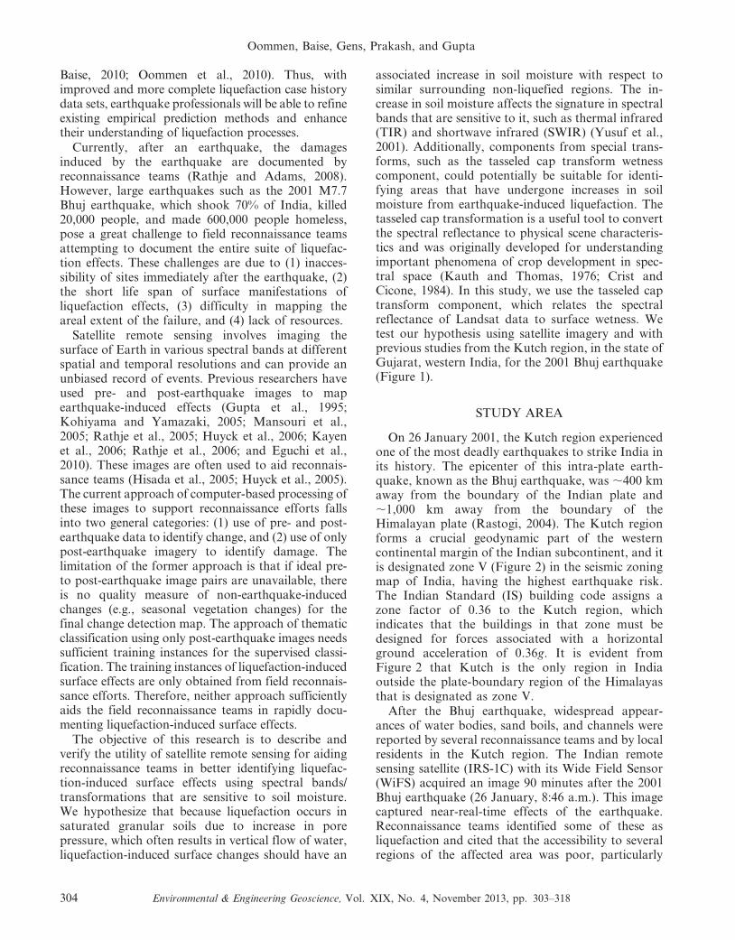
associated increase in soil moisture with respect tosimilar surrounding non-liquefied regions. The in-crease in soil moisture affects the signature in spectralbands that are sensitive to it, such as thermal infrared(TIR) and shortwave infrared (SWIR) (Yusuf et al.,2001). Additionally, components from special trans-forms, such as the tasseled cap transform wetnesscomponent, could potentially be suitable for identi-fying areas that have undergone increases in soilmoisture from earthquake-induced liquefaction. Thetasseled cap transformation is a useful tool to convertthe spectral reflectance to physical scene characteris-tics and was originally developed for understandingimportant phenomena of crop development in spec-tral space (Kauth and Thomas, 1976; Crist andCicone, 1984). In this study, we use the tasseled captransform component, which relates the spectralreflectance of Landsat data to surface wetness. Wetest our hypothesis using satellite imagery and withprevious studies from the Kutch region, in the state ofGujarat, western India, for the 2001 Bhuj earthquake(Figure 1).

STUDY AREA

On 26 January 2001, the Kutch region experiencedone of the most deadly earthquakes to strike India inits history. The epicenter of this intra-plate earth-quake, known as the Bhuj earthquake, was ,400 kmaway from the boundary of the Indian plate and,1,000 km away from the boundary of theHimalayan plate (Rastogi, 2004). The Kutch regionforms a crucial geodynamic part of the westerncontinental margin of the Indian subcontinent, and itis designated zone V (Figure 2) in the seismic zoningmap of India, having the highest earthquake risk.The Indian Standard (IS) building code assigns azone factor of 0.36 to the Kutch region, whichindicates that the buildings in that zone must bedesigned for forces associated with a horizontalground acceleration of 0.36g. It is evident fromFigure 2 that Kutch is the only region in Indiaoutside the plate-boundary region of the Himalayasthat is designated as zone V.

After the Bhuj earthquake, widespread appear-ances of water bodies, sand boils, and channels werereported by several reconnaissance teams and by localresidents in the Kutch region. The Indian remotesensing satellite (IRS-1C) with its Wide Field Sensor(WiFS) acquired an image 90 minutes after the 2001Bhuj earthquake (26 January, 8:46 a.m.). This imagecaptured near-real-time effects of the earthquake.Reconnaissance teams identified some of these asliquefaction and cited that the accessibility to severalregions of the affected area was poor, particularly

Oommen, Baise, Gens, Prakash, and Gupta

304 Environmental & Engineering Geoscience, Vol. XIX, No. 4, November 2013, pp. 303–318

due to earthquake-induced damage (Bilham, 2001;Mohanty et al., 2001; Narula and Choubey, 2001;Saraf et al., 2002; Singh et al., 2002; and Ramakrish-nan et al., 2006). In this study, we use satellite images

acquired by the National Aeronautics and SpaceAdministration (NASA) Landsat Enhanced ThematicMapper to evaluate its use in mapping earthquake-induced liquefaction-related surface effects.

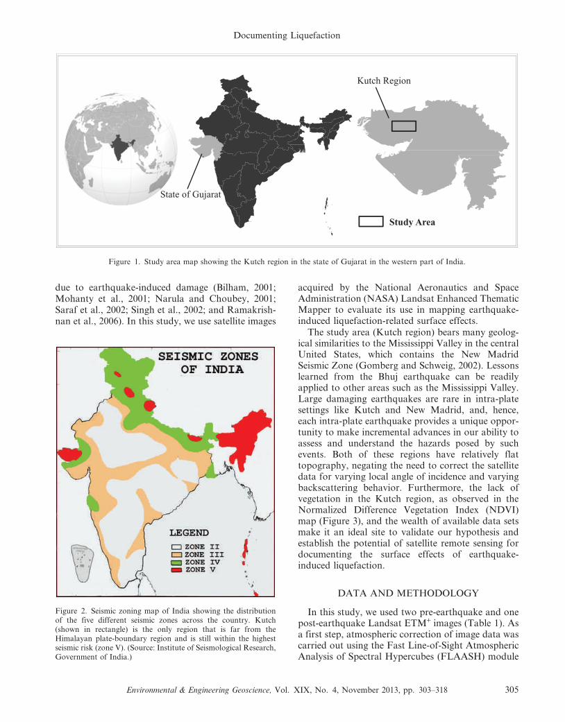
The study area (Kutch region) bears many geolog-ical similarities to the Mississippi Valley in the centralUnited States, which contains the New MadridSeismic Zone (Gomberg and Schweig, 2002). Lessonslearned from the Bhuj earthquake can be readilyapplied to other areas such as the Mississippi Valley.Large damaging earthquakes are rare in intra-platesettings like Kutch and New Madrid, and, hence,each intra-plate earthquake provides a unique oppor-tunity to make incremental advances in our ability toassess and understand the hazards posed by suchevents. Both of these regions have relatively flattopography, negating the need to correct the satellitedata for varying local angle of incidence and varyingbackscattering behavior. Furthermore, the lack ofvegetation in the Kutch region, as observed in theNormalized Difference Vegetation Index (NDVI)map (Figure 3), and the wealth of available data setsmake it an ideal site to validate our hypothesis andestablish the potential of satellite remote sensing fordocumenting the surface effects of earthquake-induced liquefaction.

DATA AND METHODOLOGY

In this study, we used two pre-earthquake and onepost-earthquake Landsat ETM+ images (Table 1). Asa first step, atmospheric correction of image data wascarried out using the Fast Line-of-Sight AtmosphericAnalysis of Spectral Hypercubes (FLAASH) module

Figure 2. Seismic zoning map of India showing the distributionof the five different seismic zones across the country. Kutch(shown in rectangle) is the only region that is far from theHimalayan plate-boundary region and is still within the highestseismic risk (zone V). (Source: Institute of Seismological Research,Government of India.)

Figure 1. Study area map showing the Kutch region in the state of Gujarat in the western part of India.

Documenting Liquefaction


of the Environment for Visualizing Images (ENVI).All other data-processing steps were carried out usingthe Erdas Imagine software package. Field data for thestudy area were limited, at best. We used the tasseledcap transform wetness component of the Landsatimage and the land surface temperature (LST) derivedfrom the thermal band as a proxy for soil moisture. Tomap the change in soil moisture, we calculated thechange in the tasseled cap transform wetness compo-nent between the pre- and post-earthquake images.

A direct change detection through subtraction ofpre- and post-earthquake images captures changesdue to the earthquake and other non-earthquake-related changes (e.g., seasonal changes). If the pre-and post-earthquake images are very closely spaced intime (difference on the order of days), the seasonalinfluence is disregarded, and the detected changes areattributed to the earthquake event. For the Bhujearthquake, we had an ideally timed data setconsisting of a January pre-earthquake image and aFebruary post-earthquake image. Unfortunately, theJanuary image was cloudy over large parts of thestudy area, and the effect of the cloud cover could notbe completely removed through atmospheric correc-tion and digital processing techniques. We therefore

relied on the November pre-earthquake images forthe change detection.

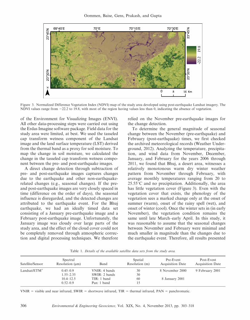
To determine the general magnitude of seasonalchange between the November (pre-earthquake) andFebruary (post-earthquake) times, we first checkedthe archived meteorological records (Weather Under-ground, 2012). Analyzing the temperature, precipita-tion, and wind data from November, December,January, and February for the years 2006 through2011, we found that Bhuj, a desert area, witnesses arelatively monotonous warm dry winter weatherpattern from November through February, withaverage monthly temperatures ranging from 20 to25.55uC and no precipitation. Additionally, the areahas little vegetation cover (Figure 3). Even with thevegetation cover that exists, the phenology of thevegetation sees a marked change only at the onset ofsummer (warm), onset of the rainy spell (wet), andonset of winter (cool). Once the winter sets in (in earlyNovember), the vegetation condition remains thesame until late March–early April. In this study, itwas reasonable to assume that the seasonal changesbetween November and February were minimal andmuch smaller in magnitude than the changes due tothe earthquake event. Therefore, all results presented

Figure 3. Normalized Difference Vegetation Index (NDVI) map of the study area developed using post-earthquake Landsat imagery. TheNDVI values range from 222.2 to 19.8, with most of the region having values less than 0, indicating the absence of vegetation.

Table 1. Details of the available satellite data sets from the study area.

Satellite/SensorSpectral

Resolution (mm) BandSpatial

Resolution (m)Pre-Event

Acquisition DatePost-Event

Acquisition Date

Landsat/ETM+ 0.45–0.9 VNIR: 4 bands 30 8 November 2000 9 February 20011.55–2.35 SWIR: 2 bands 3010.4–12.5 TIR: 1 band 60 8 January 20010.52–0.9 Pan: 1 band 15

VNIR 5 visible and near infrared, SWIR 5 shortwave infrared, TIR 5 thermal infrared, PAN 5 panchromatic.



later in the paper are direct change detection betweenthe November and February images.

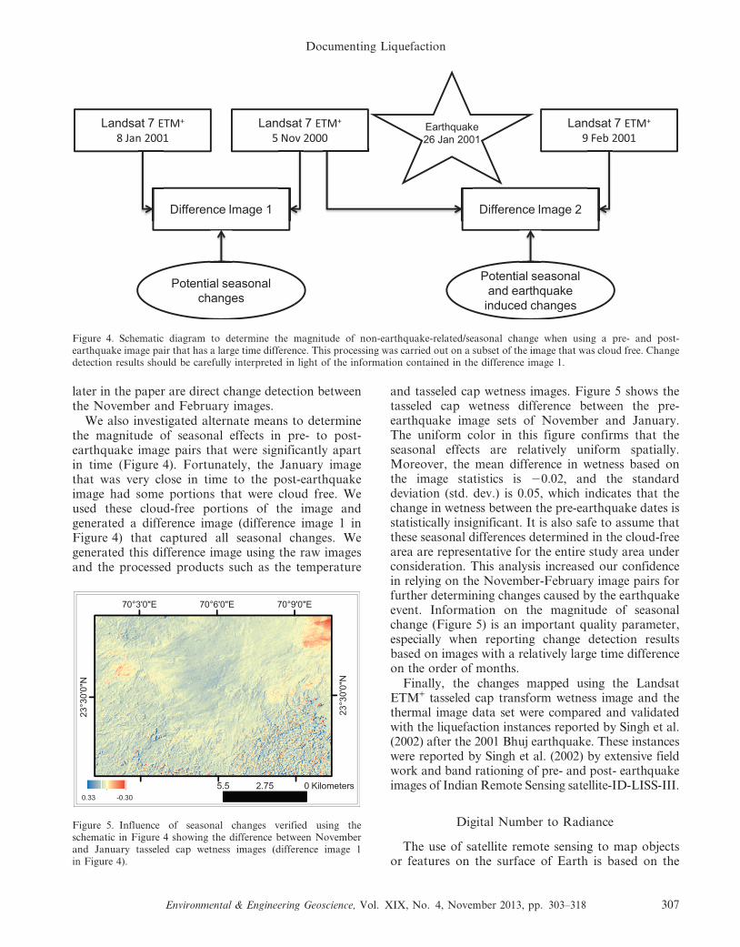
We also investigated alternate means to determinethe magnitude of seasonal effects in pre- to post-earthquake image pairs that were significantly apartin time (Figure 4). Fortunately, the January imagethat was very close in time to the post-earthquakeimage had some portions that were cloud free. Weused these cloud-free portions of the image andgenerated a difference image (difference image 1 inFigure 4) that captured all seasonal changes. Wegenerated this difference image using the raw imagesand the processed products such as the temperature

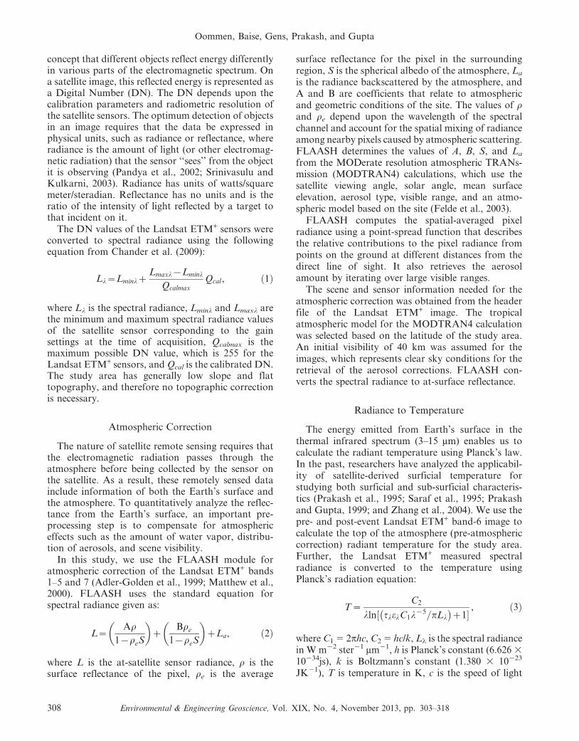
and tasseled cap wetness images. Figure 5 shows thetasseled cap wetness difference between the pre-earthquake image sets of November and January.The uniform color in this figure confirms that theseasonal effects are relatively uniform spatially.Moreover, the mean difference in wetness based onthe image statistics is 20.02, and the standarddeviation (std. dev.) is 0.05, which indicates that thechange in wetness between the pre-earthquake dates isstatistically insignificant. It is also safe to assume thatthese seasonal differences determined in the cloud-freearea are representative for the entire study area underconsideration. This analysis increased our confidencein relying on the November-February image pairs forfurther determining changes caused by the earthquakeevent. Information on the magnitude of seasonalchange (Figure 5) is an important quality parameter,especially when reporting change detection resultsbased on images with a relatively large time differenceon the order of months.

Finally, the changes mapped using the LandsatETM+ tasseled cap transform wetness image and thethermal image data set were compared and validatedwith the liquefaction instances reported by Singh et al.(2002) after the 2001 Bhuj earthquake. These instanceswere reported by Singh et al. (2002) by extensive fieldwork and band rationing of pre- and post- earthquakeimages of Indian Remote Sensing satellite-ID-LISS-III.

Digital Number to Radiance

The use of satellite remote sensing to map objectsor features on the surface of Earth is based on the

Figure 4. Schematic diagram to determine the magnitude of non-earthquake-related/seasonal change when using a pre- and post-earthquake image pair that has a large time difference. This processing was carried out on a subset of the image that was cloud free. Changedetection results should be carefully interpreted in light of the information contained in the difference image 1.

Figure 5. Influence of seasonal changes verified using theschematic in Figure 4 showing the difference between Novemberand January tasseled cap wetness images (difference image 1in Figure 4).



concept that different objects reflect energy differentlyin various parts of the electromagnetic spectrum. Ona satellite image, this reflected energy is represented asa Digital Number (DN). The DN depends upon thecalibration parameters and radiometric resolution ofthe satellite sensors. The optimum detection of objectsin an image requires that the data be expressed inphysical units, such as radiance or reflectance, whereradiance is the amount of light (or other electromag-netic radiation) that the sensor ‘‘sees’’ from the objectit is observing (Pandya et al., 2002; Srinivasulu andKulkarni, 2003). Radiance has units of watts/squaremeter/steradian. Reflectance has no units and is theratio of the intensity of light reflected by a target tothat incident on it.

The DN values of the Landsat ETM+ sensors wereconverted to spectral radiance using the followingequation from Chander et al. (2009):

Ll~LminlzLmaxl{Lminl

Qcalmax

Qcal , ð1Þ

where Ll is the spectral radiance, Lminl and Lmaxl arethe minimum and maximum spectral radiance valuesof the satellite sensor corresponding to the gainsettings at the time of acquisition, Qcalmax is themaximum possible DN value, which is 255 for theLandsat ETM+ sensors, and Qcal is the calibrated DN.The study area has generally low slope and flattopography, and therefore no topographic correctionis necessary.

Atmospheric Correction

The nature of satellite remote sensing requires thatthe electromagnetic radiation passes through theatmosphere before being collected by the sensor onthe satellite. As a result, these remotely sensed datainclude information of both the Earth’s surface andthe atmosphere. To quantitatively analyze the reflec-tance from the Earth’s surface, an important pre-processing step is to compensate for atmosphericeffects such as the amount of water vapor, distribu-tion of aerosols, and scene visibility.

In this study, we use the FLAASH module foratmospheric correction of the Landsat ETM+ bands1–5 and 7 (Adler-Golden et al., 1999; Matthew et al.,2000). FLAASH uses the standard equation forspectral radiance given as:

L~Ar

1{reS

� �z

Bre

1{reS

� �zLa, ð2Þ

where L is the at-satellite sensor radiance, r is thesurface reflectance of the pixel, re is the average

surface reflectance for the pixel in the surroundingregion, S is the spherical albedo of the atmosphere, La

is the radiance backscattered by the atmosphere, andA and B are coefficients that relate to atmosphericand geometric conditions of the site. The values of rand re depend upon the wavelength of the spectralchannel and account for the spatial mixing of radianceamong nearby pixels caused by atmospheric scattering.FLAASH determines the values of A, B, S, and La

from the MODerate resolution atmospheric TRANs-mission (MODTRAN4) calculations, which use thesatellite viewing angle, solar angle, mean surfaceelevation, aerosol type, visible range, and an atmo-spheric model based on the site (Felde et al., 2003).

FLAASH computes the spatial-averaged pixelradiance using a point-spread function that describesthe relative contributions to the pixel radiance frompoints on the ground at different distances from thedirect line of sight. It also retrieves the aerosolamount by iterating over large visible ranges.

The scene and sensor information needed for theatmospheric correction was obtained from the headerfile of the Landsat ETM+ image. The tropicalatmospheric model for the MODTRAN4 calculationwas selected based on the latitude of the study area.An initial visibility of 40 km was assumed for theimages, which represents clear sky conditions for theretrieval of the aerosol corrections. FLAASH con-verts the spectral radiance to at-surface reflectance.

Radiance to Temperature

The energy emitted from Earth’s surface in thethermal infrared spectrum (3–15 mm) enables us tocalculate the radiant temperature using Planck’s law.In the past, researchers have analyzed the applicabil-ity of satellite-derived surficial temperature forstudying both surficial and sub-surficial characteris-tics (Prakash et al., 1995; Saraf et al., 1995; Prakashand Gupta, 1999; and Zhang et al., 2004). We use thepre- and post-event Landsat ETM+ band-6 image tocalculate the top of the atmosphere (pre-atmosphericcorrection) radiant temperature for the study area.Further, the Landsat ETM+ measured spectralradiance is converted to the temperature usingPlanck’s radiation equation:

T~C2

lln½ tlelC1l{5=pLl

� �z1�

, ð3Þ

where C1 5 2phc, C2 5 hc/k, Ll is the spectral radiancein W m22 ster21 mm21, h is Planck’s constant (6.626 3

10234js), k is Boltzmann’s constant (1.380 3 10223

JK21), T is temperature in K, c is the speed of light



(2.998 3 108 ms21), tl is the atmospheric transmit-tance, and el is the spectral emissivity.

Equation 3 can be simplified for Landsat ETM+ as:

T~K2

ln K1

Llz1

� �{273, ð4Þ

where K15 666.09 W m22 ster21 mm21, K2 5

1260.56 K, and T is the temperature in uC (Chanderet al., 2009).

Land surface temperature (LST) is a valuablediagnostic of soil moisture measurement because soilsurface temperature increases with decreasing soilwater content (less evaporative cooling), while mois-ture depletion in the plant root zone results instomatal closure, reduced transpiration, and elevatedcanopy temperatures (Anderson et al., 2007; Eltahir,1998; and Vicente-Serrano et al., 2004). Shih andJordan (1993) found a coefficient of correlation (r) of0.84 between LST and soil moisture content.

Tasseled Cap Transformation

In this study, we use the tasseled cap transformationcoefficients for Landsat ETM+ reflectance developedby Huang et al. (2002) (Table 2). Huang et al. (2002)developed this transformation using several-hundredfield observations of soil, impervious surfaces, densevegetation, and moisture content. The field data wereused to determine the rotation of the principal axesobtained from principal component analysis (PCA) bypreserving its orthogonality. The technique utilizes aGram-Schmidt sequential orthogonal transformation(Huang et al., 2002). The difference between tasseledcap and PCA is that while PCA places an a priori orderon the principal directions in the data, the Gram-Schmidt approach allows the user to choose the orderof the calculation based on a physical interpretation ofthe image. This transformation converts the LandsatETM+ band (bands 1–5, 7) reflectance into six axes, ofwhich three major axes correspond to physicalcharacteristics such as brightness, greenness, andwetness. We make use of the Landsat ETM+ imagetasseled cap transform wetness axes to evaluate the

increase in surface wetness/moisture content betweenthe pre- and post-earthquake coverage.

Change Detection

An important application of satellite remotesensing data is to detect changes occurring on thesurface of Earth. Change detection methods can becategorized broadly as either supervised or unsuper-vised according to the nature of the data-processingtechnique applied (Lu et al., 2004). Supervised changedetection is based on a supervised classification method,which requires the availability of a ground truth in orderto derive a suitable training set for the learning processof the classifier, whereas the unsupervised changedetection approach performs change detection bymaking a direct comparison of the pre- and post-earthquake images. Unsupervised change detection ismainly carried out using one of the following: (1) imagedifferencing, (2) image ratioing, (3) change vectoranalysis, or (4) PCA. These change detection techniqueshave been reviewed by several researchers (Singh, 1989;Mouat et al., 1993; Deer, 1995; Coppin and Bauer,1996; Jensen et al., 1997; Prakash and Gupta, 1998;Serpico and Bruzzone, 1999; and Yuan et al., 1999). Inthis study, the unsupervised change detection isperformed by image differencing as follows:

D(x)~I2(x){I1(x), ð5Þ

where D(x) is the difference image, I2(x) is the post-earthquake image, and I1(x) is the pre-earthquakeimage. The image differencing results in positive andnegative values in areas of surface change and near-zerovalues in areas of no change. The difference image oftenproduces a distribution that is approximately Gaussianin nature, with pixels of no change distributed aroundthe mean and changed pixels distributed in the tails ofthe distribution (Gupta, 2003). A necessary pre-processing step before image differencing is normaliza-tion or standardization to reduce the inherent variabil-ity between the multi-temporal data sets (pre- and post-earthquake image) (Warner and Chen, 2001). In thisstudy, image standardization is applied before imagedifferencing. A change class map was developed from

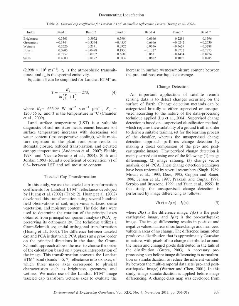
Table 2. Tasseled cap coefficients for Landsat ETM+ at-satellite reflectance (source: Huang et al., 2002).

Index Band 1 Band 2 Band 3 Band 4 Band 5 Band 7

Brightness 0.3561 0.3972 0.3904 0.6966 0.2286 0.1596Greenness 20.3344 20.3544 20.4556 0.6966 20.0242 20.2630Wetness 0.2626 0.2141 0.0926 0.0656 20.7629 20.5388Fourth 0.0805 20.0498 0.1950 20.1327 0.5752 20.7775Fifth 20.7252 20.0202 0.6683 0.0631 20.1494 20.0274Sixth 0.4000 20.8172 0.3832 0.0602 20.1095 0.0985



the difference image by simply thresholding it accord-ing to the following decision rule:

B xð Þ~1, if D xð Þj jwt

0, otherwise

�, ð6Þ

where B(x) denotes the change map, and t denotes thethreshold. The minimum number of change classes in achange map is two (i.e., positive and negative change

classes). In this study, we used 11 change classes withfive positive change classes, five negative changeclasses, and one no-change class, with the thresholdsbeing evenly spaced between 21 and +1.

ANALYSIS RESULTS AND DISCUSSION

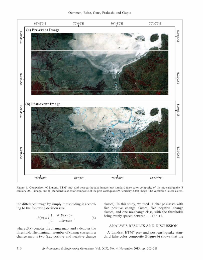
A Landsat ETM+ pre- and post-earthquake stan-dard false color composite (Figure 6) shows that the

Figure 6. Comparison of Landsat ETM+ pre- and post-earthquake images: (a) standard false color composite of the pre-earthquake (8January 2001) image, and (b) standard false color composite of the post-earthquake (9 February 2001) image. The vegetation is seen as red.



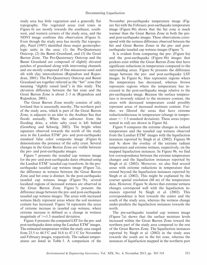
study area has little vegetation and a generally flattopography. The vegetated areas (red tones inFigure 6) are mostly towards the southeast, south-west, and western corners of the study area, and theNDVI image confirms this observation (Figure 3).Even though the study area has mostly flat topogra-phy, Patel (1997) identified three major geomorpho-logic units in the area: (1) the Pre-QuaternaryOutcrop, (2) the Banni Grassland, and (3) the GreatBarren Zone. The Pre-Quaternary Outcrop and theBanni Grassland are composed of slightly elevatedpatches of grassland along with intervening channelsand are mostly composed of fine micaceous sand andsilt with clay intercalations (Rajendran and Rajen-dran, 2001). The Pre-Quaternary Outcrop and BanniGrassland are together referred as the ‘‘bet’’ zone (betmeaning ‘‘slightly raised land’’) in this study. Theelevation difference between the bet zone and theGreat Barren Zone is about 2–3 m (Rajendran andRajendran, 2001).

The Great Barren Zone mostly consists of saltylowland that is seasonally marshy. The northern partof the study area, which is part of the Great BarrenZone, is adjacent to an inlet to the Arabian Sea thatfloods annually. When the saltwater from theflooding dries, a white salty crust is left behind(Gomberg and Schweig, 2002). The bright whitesignature observed towards the north of the studyarea in the Landsat ETM+ pre- and post-earthquakestandard false color composite image (Figure 6)demonstrates the presence of the salty crust. Severalchanges in the Great Barren Zone are visible betweenthe pre- and post-earthquake images.

Figure 7 presents the tasseled cap wetness imagefor the pre- and post-earthquake dates obtained usingthe Landsat ETM+ tasseled cap transform. In the pre-earthquake tasseled cap wetness image (Figure 7a),the difference in wetness between the Great BarrenZone and bet zone is distinct. In the post-earthquaketasseled cap wetness image (Figure 7b), severallocalized regions of increased wetness are observed inthe Great Barren Zone. Figure 7c presents thedifference image between the pre- and post-earthquaketasseled cap wetness images. The areas with increasedwetness likely represent areas where the soil moisturecontent has increased. Figure 7d represents the areasof extreme increase in tasseled cap wetness, whereextreme increase is defined as a change in wetnessmagnitude of .+1.5 standard deviation.

Figure 8 presents the computed LST for the pre- andpost-earthquake dates using the Landsat ETM+ images.The estimated temperature within the study area rangedfrom 23.5 to 44.5uC and 16.8 to 47.1uC for Novemberand February images, respectively. The radiant temper-atures are listed in Table 3. A comparison of the

November pre-earthquake temperature image (Fig-ure 8a) with the February post-earthquake temperatureimage (Figure 8b) shows that the bet zone is muchwarmer than the Great Barren Zone in both the pre-and post-earthquake images. These observations corre-spond with the wetness difference observed between thebet and Great Barren Zones in the pre- and post-earthquake tasseled cap wetness images (Figure 7).

It is evident from comparing the pre- (Figure 8a)and the post-earthquake (Figure 8b) images thatpockets exist within the Great Barren Zone that havesignificant reductions in temperature compared to thesurrounding areas. Figure 8c presents the differenceimage between the pre- and post-earthquake LSTimages. In Figure 8c, blue represents regions wherethe temperature has decreased, whereas brownrepresents regions where the temperature has in-creased in the post-earthquake image relative to thepre-earthquake image. Because the surface tempera-ture is inversely related to the moisture content, theareas with decreased temperature could possiblyrepresent areas of increased moisture content. Fur-ther, we filtered the areas that have extremereduction/decrease in temperature (change in temper-ature ,21.5 standard deviation). These areas (repre-sented in red) are shown in Figure 8d.

Figure 9 compares the extreme changes in radianttemperature and the tasseled cap wetness observedfrom the Landsat ETM+ images with the liquefactioninstances reported by Singh et al. (2002). Figures 9band 9c show the overlay of the extreme radianttemperature and extreme wetness, respectively, on themapped liquefaction instances. In Figure 9b, we findlow correspondence between the extreme temperaturechanges and the liquefaction instances reported bySingh et al. (2002). Moreover, we also find severalareas with extreme reductions in temperature thatextend beyond the liquefaction instances reported bySingh et al. (2002). This might be explained by thecoarser spatial resolution (60 m) of the temperaturedata. However, Figure 9c shows that extreme wetnesschanges correspond well with the liquefaction in-stances reported by Singh et al. (2002). Thiscorrespondence is best towards the center and thesouth of the study area, whereas the wetness changeunder-predicts the liquefaction instances towards thenorth.

The pre-earthquake tasseled cap wetness image(Figure 7a) shows that the surface moisture levelsincreased within the Great Barren Zone toward thenorthern part of the study area compared to the restof the Great Barren Zone. The liquefaction instancesreported by Singh et al. (2002) in the study areatowards the south are in the bet zone, whereas theinstances of liquefaction mapped in the northern part



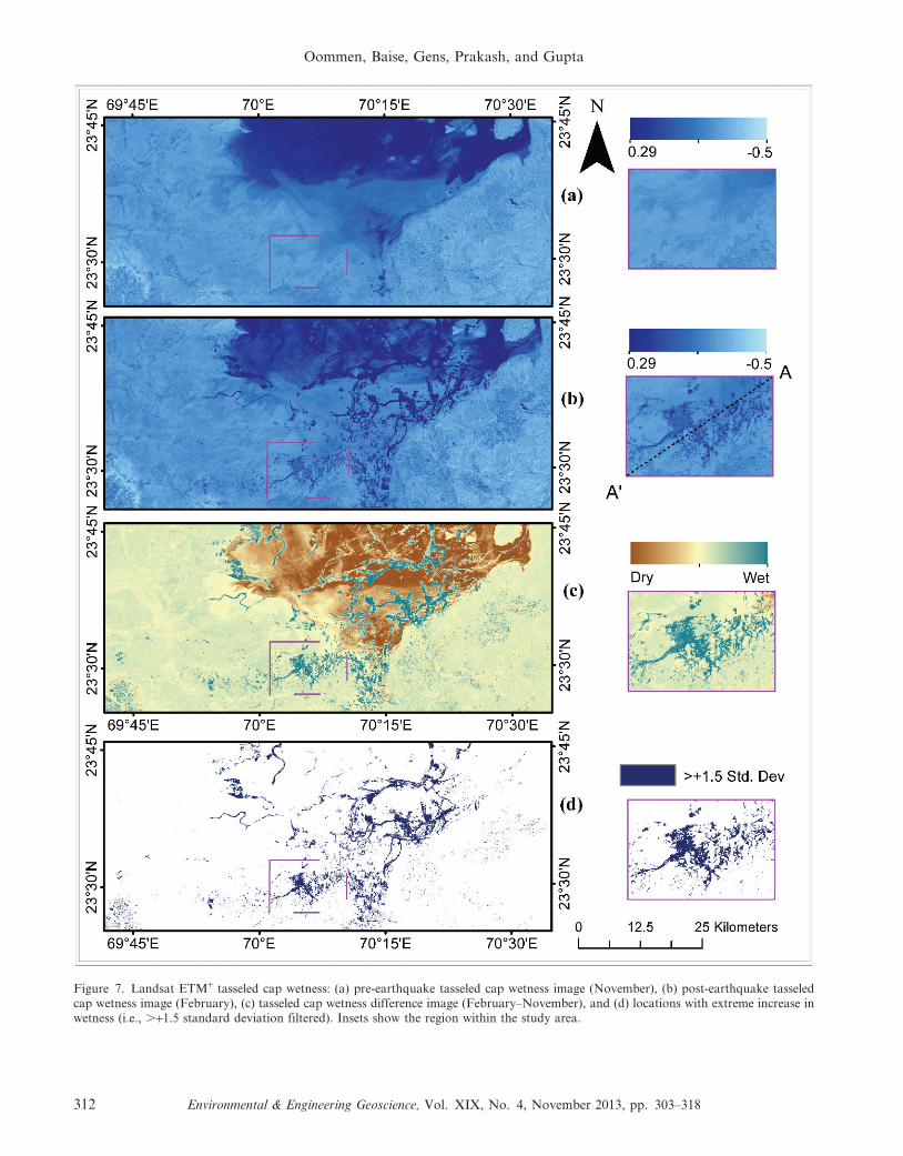
Figure 7. Landsat ETM+ tasseled cap wetness: (a) pre-earthquake tasseled cap wetness image (November), (b) post-earthquake tasseledcap wetness image (February), (c) tasseled cap wetness difference image (February–November), and (d) locations with extreme increase inwetness (i.e., .+1.5 standard deviation filtered). Insets show the region within the study area.



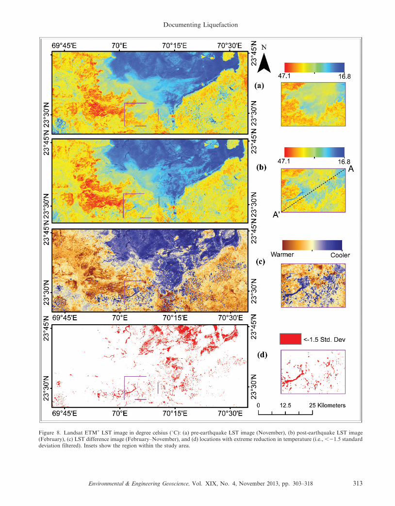
Figure 8. Landsat ETM+ LST image in degree celsius (uC): (a) pre-earthquake LST image (November), (b) post-earthquake LST image(February), (c) LST difference image (February–November), and (d) locations with extreme reduction in temperature (i.e., ,21.5 standarddeviation filtered). Insets show the region within the study area.



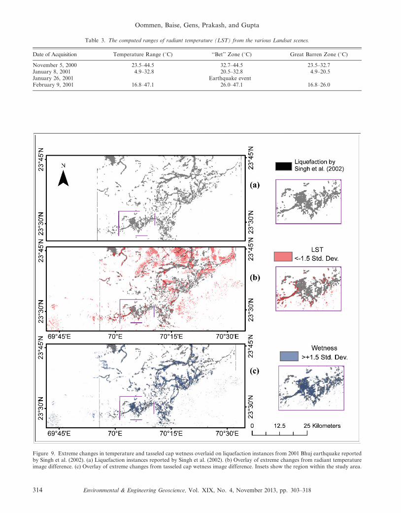
Table 3. The computed ranges of radiant temperature (LST) from the various Landsat scenes.

Date of Acquisition Temperature Range (uC) ‘‘Bet’’ Zone (uC) Great Barren Zone (uC)

November 5, 2000 23.5–44.5 32.7–44.5 23.5–32.7January 8, 2001 4.9–32.8 20.5–32.8 4.9–20.5January 26, 2001 Earthquake eventFebruary 9, 2001 16.8–47.1 26.0–47.1 16.8–26.0

Figure 9. Extreme changes in temperature and tasseled cap wetness overlaid on liquefaction instances from 2001 Bhuj earthquake reportedby Singh et al. (2002). (a) Liquefaction instances reported by Singh et al. (2002). (b) Overlay of extreme changes from radiant temperatureimage difference. (c) Overlay of extreme changes from tasseled cap wetness image difference. Insets show the region within the study area.



of the study area are in the Great Barren Zone. Thereason why the liquefaction instances within theGreat Barren Zone in the north are not identifiedwell from the extreme changes is probably because thesoil in the north is already wet, and the magnitude ofchange in wetness is smaller compared to the southernregion. This could also be related to the soil retentioncapacity of the geomorphological units. Therefore,incorporating the pre-earthquake variability in mois-ture content and the variability in soil moistureretention capacity of the geomorphological units, andfiltering the extreme changes based on these charac-teristics will be critical when using remote sensing tomap earthquake-induced liquefaction.

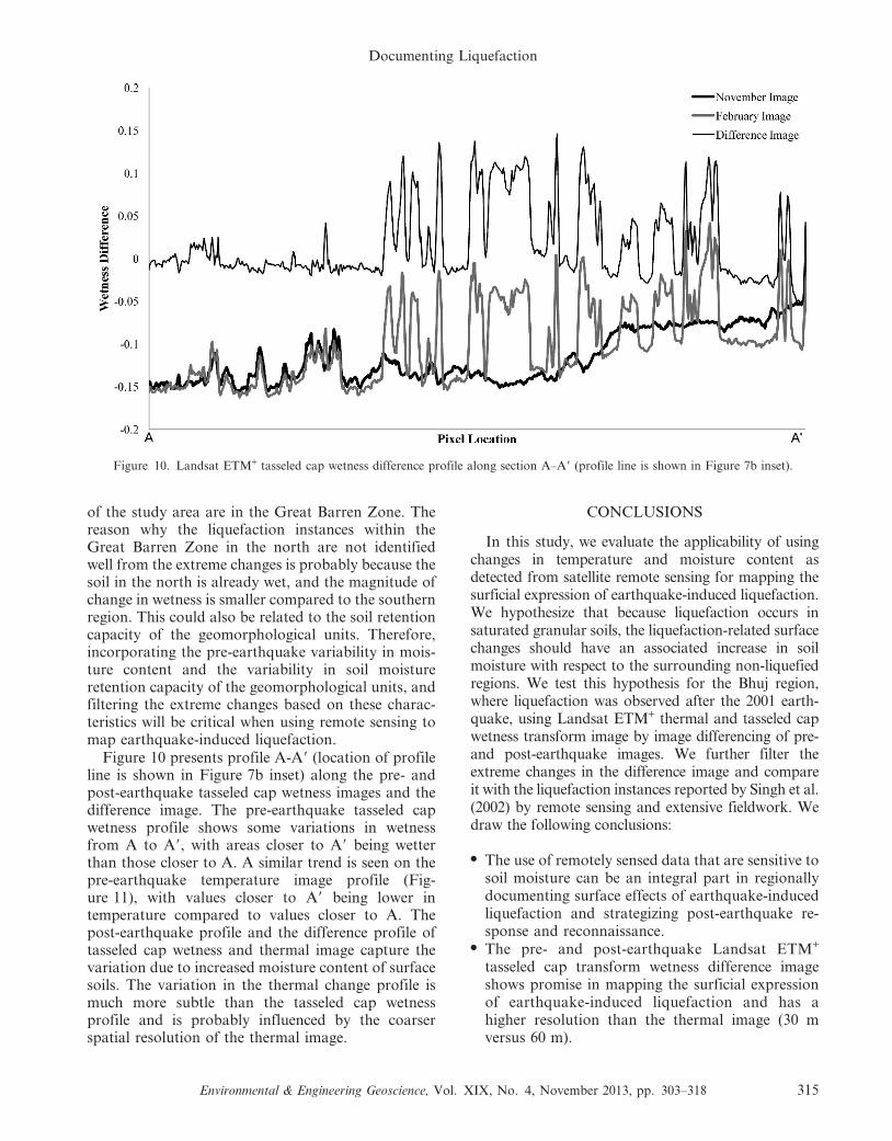
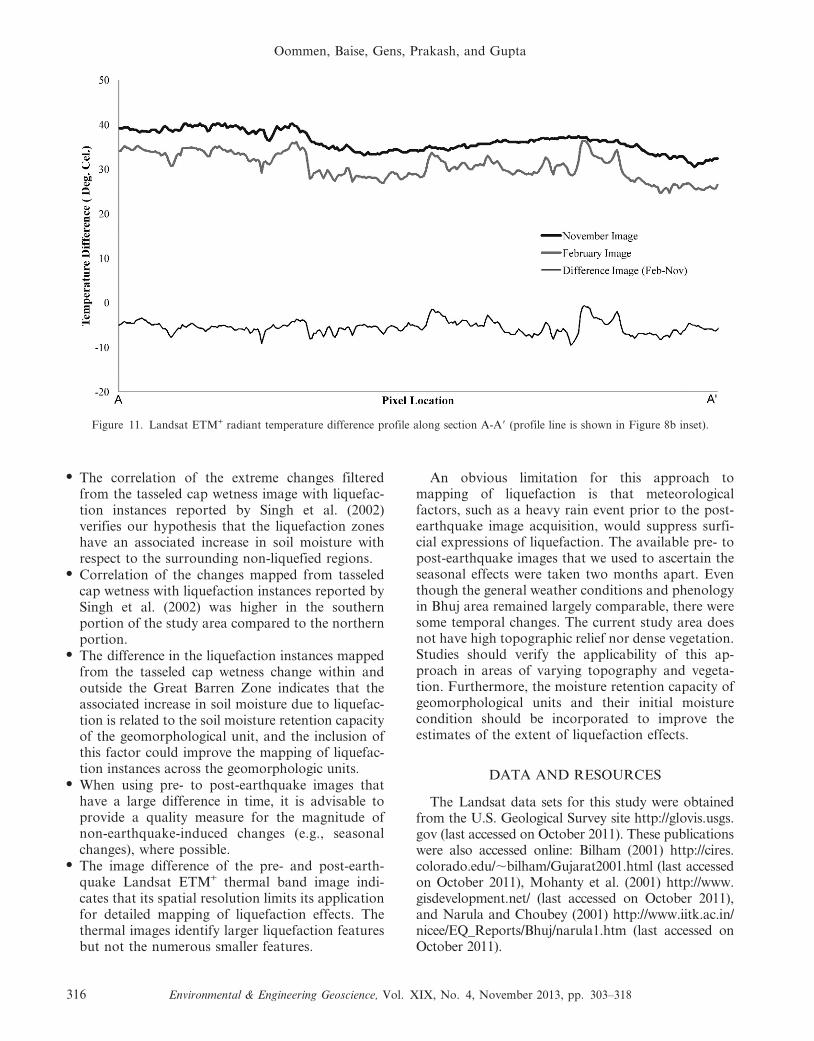
Figure 10 presents profile A-A9 (location of profileline is shown in Figure 7b inset) along the pre- andpost-earthquake tasseled cap wetness images and thedifference image. The pre-earthquake tasseled capwetness profile shows some variations in wetnessfrom A to A9, with areas closer to A9 being wetterthan those closer to A. A similar trend is seen on thepre-earthquake temperature image profile (Fig-ure 11), with values closer to A9 being lower intemperature compared to values closer to A. Thepost-earthquake profile and the difference profile oftasseled cap wetness and thermal image capture thevariation due to increased moisture content of surfacesoils. The variation in the thermal change profile ismuch more subtle than the tasseled cap wetnessprofile and is probably influenced by the coarserspatial resolution of the thermal image.

CONCLUSIONS

In this study, we evaluate the applicability of usingchanges in temperature and moisture content asdetected from satellite remote sensing for mapping thesurficial expression of earthquake-induced liquefaction.We hypothesize that because liquefaction occurs insaturated granular soils, the liquefaction-related surfacechanges should have an associated increase in soilmoisture with respect to the surrounding non-liquefiedregions. We test this hypothesis for the Bhuj region,where liquefaction was observed after the 2001 earth-quake, using Landsat ETM+ thermal and tasseled capwetness transform image by image differencing of pre-and post-earthquake images. We further filter theextreme changes in the difference image and compareit with the liquefaction instances reported by Singh et al.(2002) by remote sensing and extensive fieldwork. Wedraw the following conclusions:

N The use of remotely sensed data that are sensitive tosoil moisture can be an integral part in regionallydocumenting surface effects of earthquake-inducedliquefaction and strategizing post-earthquake re-sponse and reconnaissance.

N The pre- and post-earthquake Landsat ETM+

tasseled cap transform wetness difference imageshows promise in mapping the surficial expressionof earthquake-induced liquefaction and has ahigher resolution than the thermal image (30 mversus 60 m).

Figure 10. Landsat ETM+ tasseled cap wetness difference profile along section A–A9 (profile line is shown in Figure 7b inset).



N The correlation of the extreme changes filteredfrom the tasseled cap wetness image with liquefac-tion instances reported by Singh et al. (2002)verifies our hypothesis that the liquefaction zoneshave an associated increase in soil moisture withrespect to the surrounding non-liquefied regions.

N Correlation of the changes mapped from tasseledcap wetness with liquefaction instances reported bySingh et al. (2002) was higher in the southernportion of the study area compared to the northernportion.

N The difference in the liquefaction instances mappedfrom the tasseled cap wetness change within andoutside the Great Barren Zone indicates that theassociated increase in soil moisture due to liquefac-tion is related to the soil moisture retention capacityof the geomorphological unit, and the inclusion ofthis factor could improve the mapping of liquefac-tion instances across the geomorphologic units.

N When using pre- to post-earthquake images thathave a large difference in time, it is advisable toprovide a quality measure for the magnitude ofnon-earthquake-induced changes (e.g., seasonalchanges), where possible.

N The image difference of the pre- and post-earth-quake Landsat ETM+ thermal band image indi-cates that its spatial resolution limits its applicationfor detailed mapping of liquefaction effects. Thethermal images identify larger liquefaction featuresbut not the numerous smaller features.

An obvious limitation for this approach tomapping of liquefaction is that meteorologicalfactors, such as a heavy rain event prior to the post-earthquake image acquisition, would suppress surfi-cial expressions of liquefaction. The available pre- topost-earthquake images that we used to ascertain theseasonal effects were taken two months apart. Eventhough the general weather conditions and phenologyin Bhuj area remained largely comparable, there weresome temporal changes. The current study area doesnot have high topographic relief nor dense vegetation.Studies should verify the applicability of this ap-proach in areas of varying topography and vegeta-tion. Furthermore, the moisture retention capacity ofgeomorphological units and their initial moisturecondition should be incorporated to improve theestimates of the extent of liquefaction effects.

DATA AND RESOURCES

The Landsat data sets for this study were obtainedfrom the U.S. Geological Survey site http://glovis.usgs.gov (last accessed on October 2011). These publicationswere also accessed online: Bilham (2001) http://cires.colorado.edu/,bilham/Gujarat2001.html (last accessedon October 2011), Mohanty et al. (2001) http://www.gisdevelopment.net/ (last accessed on October 2011),and Narula and Choubey (2001) http://www.iitk.ac.in/nicee/EQ_Reports/Bhuj/narula1.htm (last accessed onOctober 2011).

Figure 11. Landsat ETM+ radiant temperature difference profile along section A-A9 (profile line is shown in Figure 8b inset).



ACKNOWLEDGMENTS

This research was supported by the U.S. GeologicalSurvey, Department of the Interior, National Earth-quake Hazards Reduction Program (NEHRP)through awards G10AP00025 and G10AP00026.The views and conclusions contained in this docu-ment are those of the authors and should not beinterpreted as necessarily representing the official poli-cies, either expressed or implied, of the U.S. government.The authors sincerely thank Drs. Jeff Keaton, CharlesM. Brankman, and the unknown reviewer for theirconstructive comments and suggestions.

REFERENCES

ADLER-GOLDEN, S. M.; MATTHEW, M. W.; BERNSTEIN, L. S.;

LEVINE, R. Y.; BERK, A.; RICHTSMEIER, S. C.; ACHARYA, P. K.;

ANDERSON, G. P.; FELDE, G. W.; GARDNER, J.; HOKE, M. P.;

JEONG, L. S.; PUKALL, B.; MELLO, J.; RATKOWSKI, A.; AND

BURKE, H. H., 1999. Atmospheric Correction for Short-Wave

Spectral Imagery Based on MODTRAN4. Society of Photo-

optical Instrumentation Engineers (SPIE) Proceeding, Imag-

ing Spectrometry, Vol. 3753, pp. 61–69.

ANDERSON, M.; NORMAN, J.; MECIKALSKI, J.; OTKIN, J.; AND

KUSTAS, W., 2007, A climatological study of evapotranspira-

tion and moisture stress across the continental U.S. based on

thermal remote sensing: Journal of Geophysical Research,

Vol. 112, D10117, doi: 10.1029/2006JD007506.

BILHAM, R., 2001, 26 January 2001 Bhuj earthquake, Gujarat,

India: Electronic document, available at http://cires.colorado.

edu/,bilham/Gujarat2001.html

CHANDER, G.; MARKHAM, B.; AND HELDER, D., 2009, Summary of

current radiometric calibration coefficients for Landsat MSS,

TM, ETM+, and EO-1 ALI sensors: Remote Sensing of

Environment, Vol. 113, No. 5, pp. 893–903.

COPPIN, P. AND BAUER, M., 1996, Digital change detection in forest

ecosystem with remote sensing imagery: Remote Sensing of

Environment, Vol. 13, pp. 207–234.

CRIST, E. P. AND CICONE, R. C., 1984, A physically-based

transformation of Thematic Mapper data—The TM tasseled

cap: IEEE Transactions on Geosciences and Remote Sensing,

Vol. GE-22, No. 3, pp. 252–263.

DEER, P., 1995, Digital Change Detection Techniques in Remote

Sensing: Defence Science and Technology Organisation

Technical Report, p. 44.

EGUCHI, R. T.; GILL, S. P.; GHOSH, S.; SVEKLA, W.; ADAMS, B. J.;

EVANS, G.; TORO, J.; SAITO, K.; AND SPENCE, R., 2010, The

January 12, 2010, Haiti earthquake: A comprehensive

damage assessment using very high resolution areal imagery.

In 8th International Workshop on Remote Sensing for Disaster

Management: Tokyo Institute of Technology, Tokyo, Japan.

ELTAHIR, E. A. B., 1998, A soil moisture-rainfall feedback

mechanism: Water Resources Research, Vol. 34, No. 4,

pp. 765–776.

FELDE, G. W.; ANDERSON, G. P.; COOLEY, T. W.; MATTHEW, M.

W.; ADLER-GOLDEN, S. M.; BERK, A.; AND LEE, J., ‘‘Analysis

of Hyperion data with the FLAASH atmospheric correction

algorithm.’’ Geoscience and Remote Sensing Symposium,

2003. IGARSS ’03. Proceedings. 2003 IEEE International,

vol. 1, no., pp.90, 92. vol. 1, 21-25 July 2013. Doi: 10.1109/

IGARSS.2003.1293688

GOMBERG, J. AND SCHWEIG, E., 2002, East Meets Midwest: An

Earthquake in India Helps Hazard Assessment in the Central

United States: U.S. Geological Survey Fact Sheet (FS-007-

02).

GUPTA, R. P., 2003, Remote Sensing Geology, 2nd ed.: Springer-Verlag, Heidelberg, 656 p.

GUPTA, R. P.; CHANDER, R.; TEWARI, A. K.; AND SARAF, A. K.,

1995, Remote-sensing delineation of zones susceptible toseismically induced liquefaction in the Ganga plains:

Journal of the Geological Society of India, Vol. 46, No. 1,

pp. 75–82.

HISADA, Y.; SHIBAYAMA, A.; AND GHAYAMGHAMIAN, M. R., 2005,

Building damage and seismic intensity in Bam city from the

2003 Iran, Bam, earthquake, Bull. Earthquake ResearchInstitute (ERI), 79, pp. 81–93.

HUANG, C.; WYLIE, B.; YANG, L.; HOMER, C.; AND ZYLSTRA, G.,

2002, Derivation of a tasselled cap transformation based onLandsat 7 at satellite reflectance: International Journal of

Remote Sensing, Vol. 23, No. 8, pp. 1741–1748.

HUYCK, C.; ADAMS, B.; CHO, S.; CHUNG, H. C.; AND EGUCHI, R.,2005, Towards rapid citywide damage mapping using

neighborhood edge dissimilarities in very high-resolutionoptical satellite imagery—Application to the 2003 Bam,

Iran earthquake: Earthquake Spectra, Vol. 21, No. S1, pp. 255–

266.

HUYCK, C.; MATSUOKA, M.; TAKAHASHI, Y.; AND VU, T., 2006,

Reconnaissance technologies used after the 2004 Niigata-ken

Chuetsu, Japan, earthquake: Earthquake Spectra, Vol. 22,pp. 133–145.

JENSEN, J. R.; COWEN, D.; NARUMALANI, M.; AND HALLS, J., 1997,

Principles of change detection using digital remote sensordata. In integration of Geographic Information Systems and

Remote Sensing Star, J.L., Estes, J.E. and McGwire, K.C(Eds.), Cambridge University Press. Cambridge, pp. 37–54.

KAUTH, R. J. AND THOMAS, G. S., 1976, The tasseled cap—A

graphic description of the spectral temporal development ofagricultural crops as seen in Landsat. In Proceedings on the

Symposium on Machine Processing of Remotely Sensed Data:

West Lafayette, Indiana, LARS, Purdue University,pp. 41–51.

KAYEN, R.; PACK, R.; BAY, J.; SUGIMOTO, S.; AND TANAKA, H.,

2006, Ground-Lidar visualization of surface and structuraldeformation of the Niigata Ken Chuetsu, 23 October 2004,

earthquake: Earthquake Spectra, Vol. 22, pp. 147–162.

KOHIYAMA, M. AND YAMAZAKI, F., 2005, Damage detection for2003 Bam, Iran, earthquake using Terra-Aster satellite

imagery: Earthquake Spectra, Vol. 21, No. S1, pp. 267–274.

LU, P. D.; MAUSEL, E. B.; AND MORAN, E., 2004, Change detectiontechniques: International Journal of Remote Sensing, Vol. 25,

No. 12, pp. 2365–2407.

MANSOURI, B.; SHINOZUKA, M.; HUYCK, C.; AND HOUSHMAND, B.,

2005, Earthquake-induced change detection in the 2003 Bam,

Iran, earthquake by complex analysis using Envisat ASARdata: Earthquake Spectra, Vol. 21, pp. 275–284.

MATTHEW, M. W.; ADLER-GOLDEN, S. M.; BERK, A.; RICHTSMEIER,

S. C.; LEVINE, R. Y.; BERNSTEIN, L. S.; ACHARYA, P. K.;ANDERSON, G. P.; FELDE, G. W.; HOKE, M. P.; RATKOWSKI, A.,

BURKE, H. H.; KAISER, R. D.; AND MILLER, D. P., 2000, Status

of atmospheric correction using a MODTRAN4-bashedalgorithm. Society of Photo-optical Instrumentation Engineers

(SPIE) Proceeding, Algorithms for Multispectral, Hyperspec-tral, and Ultraspectral Imagery, VI -4049, pp. 199–207.

MOHANTY, K.; MAITI, K.; AND NAYAK, S., 2001, Change Detection

Techniques: GIS@Development, v3: Electronic document,available at http://www.gisdevelopment.net/



MOUAT, D. A.; MAHIN, G. C.; AND LANCASTER, J., 1993, Remotesensing techniques in the analysis of change detection:Geocarto International, Vol. 2, pp. 39–50.

NARULA, P. L. AND CHOUBEY, S. K., 2001, Macroseismic Surveys forthe Bhuj (India) Earthquake of 26 January 2001: Electronicdocument, available at http://www.iitk.ac.in/nicee/EQ_Reports/Bhuj/narula1.htm

OOMMEN, T. AND BAISE, L. G., 2010, Model development andvalidation for intelligent data collection for lateral spreaddisplacements: ASCE Journal of Computing in Civil Engi-neering, Vol. 24, No. 6, pp. 467–477.

OOMMEN, T.; BAISE, L. G.; AND VOGEL, R. M., 2010, Validationand application of empirical liquefaction models: ASCEJournal of Geotechnical and Geoenvironmental Engineering,Vol. 136, No. 12, pp. 1618–1633.

OOMMEN, T.; BAISE, L. G.; AND VOGEL, R., 2011, Sampling biasand class imbalance in maximum likelihood logistic regres-sion: Mathematical Geosciences, Vol. 43, No. 1, pp. 99–120.

PANDYA, M. R.; SINGH, R.; MURALI, K. R.; BABU, P. N.;KIRANKUMAR, A. S.; AND DADHWAL, V. K., 2002, Bandpasssolar exoatmospheric irradiance and Rayleigh optical thick-ness of sensors on board Indian remote sensing satellites-1B,-1C, -1D, and P4: IEEE Transactions on Geoscience andRemote Sensing, Vol. 40, No. 3, pp. 714–718.

PATEL, P. P., 1997, Ecoregions of Gujarat: Gujarat EcologyCommission 163, GERI Campus, Race Course Road,Vadodara 390 007, India.

PRAKASH, A. AND GUPTA, R. P., 1998, Land-use mapping andchange detection in a coal mining area—A case study in theJharia coalfield, India: International Journal of RemoteSensing, Vol. 19, No. 3, pp. 391–410.

PRAKASH, A. AND GUPTA, R. P., 1999, Surface fires in Jhariacoalfield, India—Their distribution and estimation of areaand temperature from TM data: International Journal ofRemote Sensing, Vol. 20, No. 10, pp. 1935–1946.

PRAKASH, A.; SASTRY, R. G. S.; GUPTA, R. P.; AND SARAF, A. K.,1995, Estimating the depth of buried hot features fromthermal IR remote sensing data—A conceptual approach:International Journal of Remote Sensing, Vol. 16, No. 13,pp. 2503–2510.

RAJENDRAN, C. P. AND RAJENDRAN, K., 2001, Characteristics ofdeformation and past seismicity associated with the 1819Kutch earthquake, northwestern India: Bulletin of theSeismological Society of America, Vol. 91, No. 3, pp. 407–426.

RAMAKRISHNAN, D.; MOHANTY, K. K.; NAYAK, S. R.; AND

CHANDRAN, R. V., 2006, Mapping the liquefaction inducedsoil moisture changes using remote sensing technique: Anattempt to map the earthquake induced liquefaction aroundBhuj, Gujarat, India: Geotechnical and Geological Engineer-ing, Vol. 24, No. 6, pp. 1581–1602.

RASTOGI, B. K., 2004, Damage due to the Mw 7.7 Kutch, India,earthquake of 2001: Tectonophysics, Vol. 390, No. 1–4, pp. 85–103.

RATHJE, E. M. AND ADAMS, B. J., 2008, The role of remote sensingin earthquake science and engineering: Opportunities andchallenges: Earthquake Spectra, Vol. 24, No. 2, pp. 471–492.

RATHJE, E. M.; CRAWFORD, M.; WOO, K.; AND NEUENSCHWANDER,A., 2005, Damage patterns from satellite images from the

2003 Bam, Iran, earthquake: Earthquake Spectra, Vol. 21,No. S1, pp. 295–307.

RATHJE, E.; KAYEN, R.; AND WOO, K. S., 2006, Remote sensingobservations of landslides and ground deformation from the2004 Niigata Ken Chuetsu earthquake: Soils and Founda-

tions, Vol. 46, No. 6, pp. 831–842.

SARAF, A. K.; PRAKASH, A.; SENGUPTA, S.; AND GUPTA, R. P., 1995,Landsat TM data for estimating ground temperature and depthof subsurface coal fire in the Jharia coalfield, India: International

Journal of Remote Sensing, Vol. 16, No. 12, pp. 2111–2124.

SARAF, A. K.; SINVHAL, A.; SINVHAL, H.; GHOSH, P.; AND SARMA,B., 2002, Satellite data reveals 26 January 2001 Kutchearthquake-induced ground changes and appearance of waterbodies: International Journal of Remote Sensing, Vol. 23, No. 9,pp. 1749–1756.

SERPICO, S. AND BRUZZONE, L., 1999, Change Detection: WorldScientific Publishing, Singapore.

SHIH, S. AND JORDAN, J., 1993, Use of Landsat Thermal-IR dataand GIS in soil-moisture assessment: Journal of Irrigation and

Drainage Engineering, Vol. 119, No. 5, pp. 868–879.

SINGH, A., 1989, Digital change detection techniques usingremotely sensed data: International Journal of Remote

Sensing, Vol. 10, No. 6, pp. 989–1003.

SINGH, R. P.; BHOI, S.; AND SAHOO, A. K., 2002, Changes observedin land and ocean after Gujarat earthquake of 26 January2001 using IRS data: International Journal of Remote Sensing,Vol. 16, No. 23, pp. 3123–3128.

SRINIVASULU, J. AND KULKARNI, A. V., 2003, Estimation of spectralreflectance of snow from IRS-1D LISS-iii sensor over theHimalayan terrain: Journal of Earth System Science,Vol. 113, No. 1, pp. 117–128.

VICENTE-SERRANO, S.; PONS-FERNANDEZ, X.; AND CUADRAT-PRATS,J., 2004, Mapping soil moisture in the Central Ebro Rivervalley (northeast Spain) with Landsat and NOAA satelliteimagery: A comparison with meteorological data: Internation-

al Journal of Remote Sensing, Vol. 25, No. 20, pp. 4325–4350.

WARNER, T. A. AND CHEN, X., 2001, Normalization of Landsatthermal imagery for the effects of solar heating andtopography: International Journal of Remote Sensing,Vol. 22, No. 5, pp. 773–788.

WEATHER UNDERGROUND, 2012, Weather Underground: Electro-nic document, available at http://www.wunderground.com/cgi-bin/findweather/hdfForecast?query5Bhuj+India

YUAN, D.; ELVIDGE, C.; AND LUNETTA, R. S., 1999, Multispectral

Methods for Land Cover Change Analysis: Lunetta, R.S.,Elvidge, C.D. (Eds), Remote Sensing Change Detection:Environmental Monitoring Methods and Applications. Tylor& Francis. London, pp. 21–39.

YUSUF, Y.; MATSUOKA, M.; AND YAMAZAKI, F., 2001, Damageassessment after 2001 Gujarat earthquake using Landsat-7satellite images: Journal of the Indian Society of Remote

Sensing, Vol. 29, No. 1, pp. 3–16.

ZHANG, G.; ROBERTSON, P.; AND BRACHMAN, R., 2004, Estimatingliquefaction-induced lateral displacements using the StandardPenetration Test or Cone Penetration Test: Journal of Geotech-

nical and Geoenvironmental Engineering, Vol. 8, No. 130,pp. 861–871.



Documents

Documenting Earthquake-Induced Liquefaction Using ...publicationslist.org/data/thomas.oommen/ref-52/Documenting... · Documenting Earthquake-Induced Liquefaction Using Satellite Remote