Embed Size (px)
Citation preview

No 2007 – 02January
Does Risk Aversion Drive Financial Crises?Testing the Predictive power of Empirical Indicators
_____________
Virginie CoudertMathieu Gex

2
Does Risk Aversion Drive Financial Crises?Testing the Predictive power of Empirical Indicators
_____________
Virginie CoudertMathieu Gex
No 2007 – 02January

Does Risk Aversion Drive Financial Crises?Testing the Predictive power of Empirical Indicators
3
TABLE OF CONTENTS
Summary...............................................................................................................................3
Abstract.................................................................................................................................5
Résumé ..................................................................................................................................6
Résumé court ........................................................................................................................8
SUMMARY ..............................................................................................................................5
ABSTRACT..............................................................................................................................6
RÉSUMÉ .................................................................................................................................7
1. INTRODUCTION ................................................................................................................9
2. THEORETICAL FRAMEWORK.........................................................................................10
2.1 Risk aversion in the CCAPM ................................................................................102.2 Consistency with the CAPM .................................................................................122.3 Consistency with factor models.............................................................................14
3. THE RISK AVERSION INDICATORS .................................................................................14
3.1 Indicators of the GRAI type ..................................................................................143.2 A PCA indicator ....................................................................................................163.3 Simple and aggregated indicators: the VIX and the LCVI ....................................173.4 Other measures: the ICI.........................................................................................183.5 Comparison of the indicators.................................................................................18
4. TESTING THE PREDICTIVE POWER OF THE INDICATORS ..............................................19
4.1 Definition of currency crises .................................................................................194.3 The dependent variable..........................................................................................224.4 The models used ....................................................................................................224.5 Assessing the predictive power .............................................................................23
5. FORECASTING OF CURRENCY CRISES............................................................................24
5.1 Significance of the control variables and the risk aversion indicators...................245.2 Predictive power for currency crises .....................................................................24
6. FORECASTING OF STOCK MARKET CRISES....................................................................25
6.1 Significance of the control variables and the risk aversion indicators...................256.2 Predictive power for stock market crises...............................................................256.3 Can stock market reversals be predicted?..............................................................26
7. CONCLUSION..................................................................................................................27

CEPII, Working Paper No 2007 - 02
4
References ...........................................................................................................................28
Appendix 1: the database ..................................................................................................38
Appendix 2: risk aversion indicators graphs ...................................................................40
Appendix 3: currency and stock market crises ...............................................................41
List of Working Papers released by CEPII......................................................................47

Working paper No 2007- 02
DOES RISK AVERSION DRIVE FINANCIAL CRISES?TESTING THE PREDICTIVE POWER OF EMPIRICAL INDICATORS
NON-TECHNICAL SUMMARY
Financial institutions often refer to empirical risk aversion indicators to gauge investors’market sentiment. Fluctuations in risk aversion are generally considered as a factorexplaining crises. Periods of strong risk appetite can create speculative bubbles on financialprices, building up vulnerabilities. Then a sudden reversal in risk aversion may triggersharp falls in asset prices and prompt a financial crisis.
A crucial point is to clearly define the concept of risk aversion. In the framework of assetpricing models, more precisely the Consumption CAPM (CCAPM), a risk premium can bedecomposed into a “price of risk”, which is common to all assets, and a “quantity of risk”,which is specific to each asset. The empirical indicators of risk aversion used by financialinstitutions aim at assessing this “price of risk”.
Those empirical indicators can be put together in four main groups. 1) The indicators of theGRAI (Global Risk Aversion Index) type are based on the idea that an increase in riskaversion should lead to a rise in risk premia across all markets, but the rise should begreater on the riskiest markets (Persaud, 1996, Kumar and Persaud, 2002). By using theCAPM, regarded as a special case of the CCAPM, this idea amounts to assessing changesin risk aversion as the correlation between price changes and their volatility. 2) Riskaversion can also be estimated as the common factor driving risk premia. This commonfactor can be evaluated through a factor analysis such as the Principal Component Analysis(PCA). 3) Some financial institutions also use raw series, as the VIX which is the impliedvolatility on the S&P 500, or combinations of raw series. 4) There are also other indicators,such as the State Street’s one which does not fall into the previous categories.
In order to assess the relevance of all these empirical indicators, we investigate their abilityto forecast exchange rate and stock market crises, by constructing “early warning signals”of crises. We use logit and multilogit models that link a qualitative variable representingcrises to a set of quantitative exogenous variables. In a first model, the explanatoryvariables are the usual ones found in the economic literature. In a second model we add riskaversion indicators to these control variables. In a third one, risk aversion indicators aretaken as the only explicative variable.
The results show that most of the considered risk aversion indicators have the expectedpositive sign and are significant in the regressions. Moreover, in the multilogit models, riskaversion remains high during the months following the crisis. As regard to their predictivepower, which is tested in-the-sample, the results are quite different according to the type ofcrises. For currency crises, the indicators barely improve the prediction made by the usualcontrol variables. By contrast, in the case of stock market crises, most indicators yieldsatisfactory results. The best predicting performances are obtained by a principalcomponent analysis on risk premia.
CEPII, Working Paper No 2007 - 02
6
ABSTRACT
Financial institutions often refer to empirical risk aversion indicators to gauge investors’market sentiment. These indicators, which are estimated in diverse ways, often showdiffering developments, although it is not possible to directly assess which is the mostappropriate. Here, we consider the most well-known of these indicators and constructothers with standard methods. As financial crises generally coincide with periods in whichrisk aversion increases, we try to check if these indicators rise just before the crises and alsoif they are able to forecast crises. We estimate logit and multilogit models of financialcrises – exchange rate and stock market crises – using control variables and each of the riskaversion indicators. In-sample simulations allow us to assess their respective predictivepowers. Risk aversion indicators are found to be good leading indicators of stock marketcrises, but less so for currency crises.
JEL Classification: C33, E44, F37, G12.
Keywords: Risk aversion; Leading indicators of crises, Currency crises, Stockmarket crises, Crises prediction.

Does Risk Aversion Drive Financial Crises?Testing the Predictive power of Empirical Indicators
7
L’AVERSION POUR LE RISQUE EXPLIQUE-T-ELLE LES CRISES FINANCIERES ?UN TEST SUR LA CAPACITÉ PRÉDICITVE DES INDICATEURS EMPIRIQUES
RÉSUMÉ NON TECHNIQUE
De nombreuses institutions financières utilisent des indicateurs d’aversion pour le risquepour évaluer l’humeur des investisseurs. Les fluctuations de l’aversion pour le risque sontsouvent considérées comme un facteur explicatif des crises. Les périodes de fort appétitpour le risque peuvent être à l’origine de bulles spéculatives sur le prix des actifs financiers,créant ainsi des vulnérabilités. Un effondrement brutal de l’optimisme des investisseurspeut ensuite conduire à une forte baisse des prix et provoquer une crise financière.
Un point déterminant consiste à définir clairement le concept d’aversion pour le risque. Lecadre théorique fourni par les modèles de détermination des prix d’actifs, et plusprécisément le Consumption CAPM (CCAPM), permet de décomposer une prime de risqueen un « prix du risque », commun à tous les actifs, et une « quantité de risque », spécifiqueà chaque actif. Les différents indicateurs que nous utilisons dans ce papier cherchent àévaluer ce « prix du risque ».
Ces indicateurs empiriques peuvent être classés en quatre groupes. 1) Les indicateurs detype GRAI (Global Risk Aversion Index) sont basés sur l’idée qu’une augmentation del’aversion pour le risque devrait conduire à une augmentation des primes de risque sur tousles marchés, cependant cette augmentation devrait être plus importante sur les marchés lesplus risqués (Persaud, 1996, Kumar et Persaud, 2002). En utilisant le CAPM, considérécomme un cas particulier du CCAPM, cette idée revient à mesurer les évolutions del’aversion pour le risque à travers la corrélation entre les variations de prix et les volatilitésde ces variations sur un panel de différents actifs. 2) Il est possible d’estimer l’aversionpour le risque comme le facteur commun à un ensemble de primes de risque. Une analysefactorielle, telle que l’Analyse en Composantes Principales (ACP) permet de mesurer cefacteur commun. 3) Quelques institutions financières utilisent également des séries brutes,comme le VIX, qui est égal à la volatilité implicite sur le S&P 500, ou des combinaisons deséries brutes. 4) D’autres indicateurs, comme celui de State Street, n’entrent dans aucunedes catégories précédentes.
Pour juger de la pertinence de ces indicateurs empiriques, nous nous intéressons à leurcapacité à prévoir les crises de change et les crises boursières, en construisant des« indicateurs avancés » de crise. Nous utilisons des modèles logit et multilogit qui relientune variable qualitative représentant la crise à un ensemble de variables quantitatives. Unpremier modèle retient pour variables explicatives les variables habituelles trouvées dans lalittérature économique. Dans un second modèle, nous ajoutons les indicateurs d’aversionpour le risque à ces variables de contrôle. Dans un troisième modèle, les indicateursd’aversion pour le risque sont utilisés comme seules variables explicatives.
Les résultats montrent que les plupart des indicateurs considérés ont le signe positif attenduet sont significatifs dans les régressions. De plus, dans les modèles multilogit, l’aversionpour le risque reste élevée durant les mois suivant la crise. Concernant leur pouvoir

CEPII, Working Paper No 2007 - 02
8
prédictif, qui est testé ici à l’intérieur de l’échantillon, les résultats sont différents selon letype de crise. Pour les crises de change, les indicateurs améliorent à peine les prévisionsobtenues avec les variables de contrôle habituelles. Dans le cas des crises boursières, laplupart des indicateurs donnent des résultats satisfaisants. Les meilleures performancessont obtenues par une ACP sur les primes de risque.
RÉSUMÉ
De nombreuses institutions financières utilisent des indicateurs d’aversion pour le risquepour évaluer l’humeur des investisseurs. Ces indicateurs, estimés de différentes façons,présentent souvent des évolutions hétérogènes sans qu’il soit possible de les départagerdirectement. Ici, nous étudions les indicateurs empiriques les plus souvent utilisés et enconstruisons d’autres à partir des méthodes les plus connues. Les crises financièrescoïncident généralement avec les périodes durant lesquelles l’aversion pour le risqueaugmente. Nous essayons donc de voir si ces indicateurs connaissent une hausse juste avantles crises et également s’ils permettent de prédire ces crises. Nous estimons des modèleslogit et multilogit des crises financières – crises de change et crises boursières – en utilisantdes variables de contrôle. Les simulations réalisées sur notre échantillon nous permettentd’évaluer leur pouvoir prédictif respectif. Les résultats obtenus incitent à conclure que lesindicateurs d’aversion pour le risque sont de bons indicateurs avancés des crises boursières,beaucoup moins pour les crises de change.
Classement JEL : C33, E44, F37, G12.
Mots Clés : Aversion pour le risque, Indicateurs avancés de crise, crises dechange, crises boursières; prévision de crise.
Does Risk Aversion Drive Financial Crises?Testing the Predictive power of Empirical Indicators
9
DOES RISK AVERSION DRIVE FINANCIAL CRISES?TESTING THE PREDICTIVE POWER OF EMPIRICAL INDICATORS
Virginie Coudert1, Mathieu Gex
2
1. INTRODUCTION
Fluctuations in investor risk aversion are often cited as a factor to explain crises onfinancial markets. The alternation between periods of optimism prompting investors tomake risky investments, and periods of pessimism, when they retreat to the safest forms ofinvestments, could be at the root of sharp fluctuations in asset prices (Borio, Kennedy andProwse, 1994). Strong “risk appetite” leading to investors’ excessive optimism can createspeculative bubbles on financial prices, building up vulnerabilities. Then a sudden reversalin risk aversion may trigger sharp falls in asset prices and prompt a financial crisis. Oneproblem in assessing the different periods, “risk appetite” or risk aversion, is clearlydistinguishing the risk perceived by agents from risk aversion itself.
Theoretically, risk aversion can be precisely defined within the framework of asset pricingmodels (Campbell, Lo and MacKinlay, 1997, Cochrane, 2001). In this context, a riskpremium can be decomposed into a “price of risk”, which is common to all assets, and a“quantity of risk” which is specific to each asset. Risk aversion can be considered as the“price of risk” obtained in this way. Other authors refer to “risk appetite”, which is just thesame “price of risk” with a negative sign (Kumar and Persaud, 2002, Gai and Vause, 2006).
Empirically, several methods have been developed in order to assess risk aversion.However, they yield indicators, which often show differing developments. The aim of thepaper is to assess their respective relevance and their ability to predict crises.
Here we consider the most well-known ones: the GRAI type indicators, introduced byKumar and Persaud (2002), based on the correlation between volatilities and changes inasset prices; indicators using a principal components analysis (PCA) on risk premia, asconstructed by Sløk and Kennedy (2004); the VIX, using implicit volatility of optionprices, created by the Chicago Board Options Exchange (CBOE, 2004); the LCVI, asynthetic indicator constructed by J.P. Morgan (Prat-Gay and McCormick, 1999, andKantor and Caglayan, 2002); the ICI, used by State Street and based on the movements ininvestors’ portfolios (Froot and O’Connell, 2003). We calculate the two first categories: theGRAI and a PCA indicator with empirical data on financial prices; we use the originalseries provided by their authors for the VIX, LCVI and ICI.
1 Banque de France, DGO, DCSF, 31 rue Croix des Petits Champs, 75001 Paris – email :[email protected] , CEPN, université Paris 13, CEPII, 9 rue Georges Pitard, 75015 Paris.
2 Banque de France, 31 rue des Petits Champs, 75001 Paris, CERAG, université Grenoble 2.

CEPII, Working Paper No 2007 - 02
10
We then test these indicators ability to forecast currency and stock market crises. Muchwork has been done to attempt to construct “leading indicators” of crises, since the Mexicancrisis in 1995 (Kaminsky, Lizondo and Reinhart, 1997, Berg and Patillo, 1999, Bussièreand Fratzscher, 2006). The idea underlying this research has been to identify economicvariables that behave in a particular way prior to periods of crisis. Their aim is to assessprobabilities of crisis at a specific horizon (generally one or two years), taking account ofthe information available on the economic variables. Most of them use logit models thatlink a qualitative endogenous variable (equal to 1 for crises and 0 for quiet periods) to a setof quantitative exogenous variables (Frankel and Rose, 1996, Sachs, Tornell and Velasco,1996, Radelet and Sachs, 1996). These models are estimated for a large number ofcountries and periods. We use the same method here, adding risk aversion indicators to theusual variables.
Section 2 theoretically states the risk aversion concept which will be used in the frameworkof standard asset pricing models (CCAPM and CAPM). Section 3 describes the empiricalmethods for constructing the risk aversion indicators. Section 4 gives the definition ofcrises for foreign exchange and stock markets; it also presents the different logit andmultilogit models used for forecasting. We successively use these models with controlvariables and/or with each risk aversion indicator. Section 5 gives the estimation results andin-sample simulations for currency crises; section 6 for stock market crises and reversals.Section 7 concludes.
2. THEORETICAL FRAMEWORK
2.1 Risk aversion in the CCAPM
The CCAPM allows to link asset prices to the consumer’s utility function. To keep itsimple, we assume that there is a single risky asset, that the agent can buy and sell freely,two periods, t and t+1, constant consumer prices and a utility function that is separable overtime. The agent’s non-financial income in period t+1 is a stochastic variable depending onthe state of the world in t+1. The agent maximises his expected utility by choosing anoptimal quantity of asset to buy in the first period, as in the following programme.
{ }( ) ( )[ ]
⎪⎪⎩
⎪⎪⎨
⎧
+=−=
+
+++
+
ξξ
δξ
111
1max
ttt
ttt
ttt
xycpyc
cuEcu
(1)
We denote consumption in t as tc , non-financial revenue as ty , the price of the asset as tp ,gross income from the asset 1+tx , and the quantity of asset bought in t as ξ. δ is theintertemporal discount factor, which captures the consumer’s preference for present.
The price of the asset tp is deduced from the first order condition:

Does Risk Aversion Drive Financial Crises?Testing the Predictive power of Empirical Indicators
11
( )( ) ⎥
⎦
⎤⎢⎣
⎡′′
= ++
11
tt
ttt x
cucuEp δ (2)
The asset price expressed in equation (2) can be interpreted as the expected income 1+tx ,discounted by a discount factor, denoted 1+tm and referred to as the “stochastic discountfactor” (SDF, thereafter):
( )11 ++= tttt xmEp (3)
with( ) ( )[ ]ttt cucum ′′= ++ 11 δ (4)
To express the risk premia, we use the gross return on the asset, dividing income 1+tx by
the price tp (i.e. ttt pxR 11 ++ = )1:
( )111 ++= tt RmE (5)
By definition, the income from a risk-free asset does not vary with states of the world,which amounts to saying that the risk-free rate in t+1, denoted f
tR 1+ , is known in advance:
( )11
1
++ =
t
ft mE
R (6)
By definition, the risk premium equals the difference ( ) ftt RRE 11 ++ − , i.e. the expected excess
return on the risky asset compared to that on the risk-free asset.
Considering equations (5) and (6), we have:
( ) ( ) fttt
ftt RRmRRE 1111 ,cov +++++ −=− (7)
The risk premium therefore equals minus the covariance of the return on the risky assetwith the SDF multiplied by the risk-free rate. It can be decomposed as follows:
( ) ( )( )
( )( ) ⎟
⎟⎠
⎞⎜⎜⎝
⎛⎟⎟⎠
⎞⎜⎜⎝
⎛−=−
+
+
+
++++
1
1
1
1111
varvar
,cov
t
t
t
ttftt mE
mm
mRRRE (8)
Generally speaking, assuming there are several assets subscripted from i = 1 to n:
( ) ( )( )
( )( ) ⎟
⎟⎠
⎞⎜⎜⎝
⎛⎟⎟⎠
⎞⎜⎜⎝
⎛−=−
+
+
+
++++
1
1
1
1111
varvar
,cov
t
t
t
titf
tit mE
mm
mRRRE (9)
1 To lighten the notation, from now on, we suppress the subscripts on Et, as well as on the variance and
covariance, for they are all calculated in time t.

CEPII, Working Paper No 2007 - 02
12
which can be written in the form:
( ) mmif
tit RRE λβ ,11 =− ++ (10)
with
( )( )1
11, var
,cov
+
++−=t
tit
mi mmR
β (11)
and
( )( )1
1var
+
+=t
tm mE
mλ (12)
We can consider that mλ is the price of risk, which is common to all assets, and that mi,β isthe specific quantity of risk associated with each asset.
Often, the price of risk mλ is regarded as corresponding to risk aversion. We do the same inthis paper. However, to avoid any confusion, it should be distinguished from the parameterof risk aversion in the consumer’s utility function. For example, using the conventional
power utility function ( ) γ
γ−
−= 1
11
tt ccu , where γ is the coefficient of relative risk aversion,
the SDF is written:
( ) γδ −++ = ttt ccm 11 . (13)
The expected return and price of risk depend on the rate of growth in consumption, denotedc∆ :
( )( )c
RRE
c
ccif
tit
∆=
+=
∆
∆∆++
var,11
γλ
λβ(14)
2.2 Consistency with the CAPM
The CCAPM model may be regarded as being a general representation from which theother models currently used to determine asset prices can be deduced. The CAPM ofSharpe (1964) and Lintner (1965a, 1965b) may be considered a particular case of theCCAPM. We therefore express the SDF depending on the return, denoted W
tR 1+ , on the
“wealth portfolio” held by the consumer. This return WR thus serves to approximate themarginal utility of consumption:
Wtt bRam 11 ++ −= (15)
Does Risk Aversion Drive Financial Crises?Testing the Predictive power of Empirical Indicators
13
a and b are parameters > 0.2
WR is proxied by the return on a broad portfolio of stocks regarded as “the marketportfolio”. The return on the market portfolio, denoted mR , equals the average return onall of the assets indexed by i = 1 to n weighted by their share iα , so that:
∑ ++ =i
iti
mt RR 11 α (16)
This assumes that the consumer’s wealth is invested across the whole of the market. If thereturn on the market portfolio is denoted mR , the SDF will then be:
mtt bRam 11 ++ −= (17)
Using equations (7) and (17) and assuming again that there are several assets, indexed byi = 1 to n, then:
( ) ( ) ( )mt
it
ft
ft
mt
it
ft
ft
it RRbRRbRaRRRRE 111111111 ,cov,cov +++++++++ +=−−= (18)
The expression of the risk premium is obtained by dividing and multiplying the right sideof equation (18) by ( )m
tR 1var + :
( ) ( ) ( )( ) ⎟⎟
⎠
⎞⎜⎜⎝
⎛+=
+
++++++ m
t
mt
itm
tf
tf
tit R
RRRbRRRE1
111111 var
,covvar (19)
Identifying to equation (6), we can write (19) in the following form, which is consistentwith the CCAPM:
( ) mmif
tit RRE λβ ,11 += ++ (20)
with
( )( )m
t
mt
it
mi RRR
1
11, var
,cov
+
++=β (21)
and
( )( )m
t
mt
m RER
b1
1var
+
+=λ (22)
2 The theoretical values of these parameters are obtained by setting: 1 = Et(mt+1 RW
t+1) et 1 = Et(mt+1)Rft+1.

CEPII, Working Paper No 2007 - 02
14
The market return plays a similar role to that of changes in consumption in the previousmodel.
2.3 Consistency with factor models
The Arbitrage Pricing Theory (APT) (Ross, 1976), based on the lack of arbitrageopportunities, relies on the assumption that yields on different securities depend on one ormore common factors which are not directly observable. APT specifies neither theirnumber nor their nature. In the framework of the CAPM, the only factor to consider is themarket return. In other models, several factors are retained. For instance, Fama and French(1996) show that a three-factor model may explain the change in excess return of US stocksportfolios. The SDF is expressed according to a number of factors f, which may be differentfrom consumption or market returns.
bfm tt '11 ++ = (23)
As the factors f are not directly observable, a factor analysis method, such as a PrincipalComponent Analysis (PCA), is needed to estimate them (see Cochrane, 2001, p. 175).
3. THE RISK AVERSION INDICATORS
3.1 Indicators of the GRAI type
An increase in risk aversion should lead to a rise in risk premia across all markets, but therise should be greater on the riskiest markets. This is the idea on which the Global RiskAversion Index (GRAI) is based, devised by Persaud (1996): changes in risk aversion maytherefore be represented by the correlation across different assets between price variationsand their volatility.
The framework is given by a CAPM model of the type that we can express as in (20), (21)and (22). If we add an assumption of independent returns on different markets, the riskpremium on each security i no longer depends on the covariance with other premia, butonly on the security’s variance (denoted 2
iσ ).
( ) ( )( ) 2
2
1
1111 var
,cov
m
iimt
iti
itf
tit R
RRRREσσαλαλ ==−
+
++++ (24)
By deriving formula (24) in relation to λ, we obtain the change in the expected riskpremium when risk aversion increases:
( )[ ]2
211
m
iif
tit RRE
σσα
λ=
∂−∂ ++ (25)
Thus, an increase in risk aversion results in an increase in the expected risk premium of theasset i that is proportional to the volatility of asset i’s return, according to equation (25).
Does Risk Aversion Drive Financial Crises?Testing the Predictive power of Empirical Indicators
15
By deriving formula (24) in relation to 2iσ , we obtain the change in the risk premium
across the different assets 1,…, n when the asset’s volatility, i.e. the risk associated with i,increases:
( )[ ]22
11
m
i
i
ft
it RRE
σλα
σ=
∂−∂ ++ (26)
Equation (26) shows that an increase in asset i’s volatility brings about an increase in therisk premium of i that is proportional to the risk aversion, but does not depend on i’svolatility.
The GRAI indicators calculated use variations in prices rather than in expected excessreturns, which explains the change in sign in the correlation.
The expected return equals the anticipated change in price:
( ) ti
tit PPERE −= ++ )( 11 (27)
By assuming that ( )itPE 1+ is constant and using (27) and (24), we obtain:
[ ]2
2
m
iitPσσα
λ−=
∂∂
(28)
The GRAI is therefore calculated as a correlation with a negative sign between pricechanges of the different assets and their volatility. By construction, the GRAI does notmeasure levels of risk aversion but rather changes in it. Spearman’s correlation is oftenused, which is a correlation between ranks of variables. Instead of a correlation, aregression coefficient between price variations and volatilities may also be used (which isalso given a negative sign). The indicator is then called the Risk Aversion Index (RAI), asproposed by Wilmot, Mielczarski and Sweeney, (2004).
In order to be entirely rigorous, confidence intervals need to be constructed around theestimated values. When this is done, GRAI indicators are often found to be in a non-significant area (more than half of the values in Kumar and Persaud’s study). However, itmust be admitted that these confidence intervals are not calculated for other empirical riskaversion indicators. Kumar and Persaud (2002) applied this approach to ex post excessreturns on foreign exchange markets, Baek et al. (2005) on developed and emerging stockmarkets. Several financial institutions and private banks, such as the IMF and J.P. Morgan,subsequently constructed their own GRAI. Other like Crédit Suisse First Boston (Wilmot,Mielczarski and Sweeney, 2004) and the Deutsche Bundesbank (2005) have constructedRAIs.
From a theoretical standpoint, the construction is based on simplifying assumptions that areprobably not borne out in reality, notably, the independence of excess returns and theindependence between expected future prices and variations in risk aversion (Misina, 2003,

CEPII, Working Paper No 2007 - 02
16
2006). From an empirical point of view, the GRAI and RAI also display some limitations.The measurements show that these indicators are very volatile. This seems counter-intuitive, as a good indicator should be stable during quiet periods. Moreover, changes inthe indicator over time differ quite markedly depending on the period chosen for thecalculations of volatility of returns as well as on the market concerned.
We calculate a GRAI and a RAI for the foreign exchange and stock markets using monthlydata. Volatility is calculated over the two previous years. For the currency GRAI, thesample comprises 12 to 15 currencies quoted against the US dollar depending on theperiods for which data are available; excess returns are equal to the spread between the 3-month forward rate and the actual spot rate three months later. For the stock market GRAI,the sample is made up of the main stock market indices of 27 developed and emergingeconomies.
3.2 A PCA indicator
As shown in section 2.3, in the framework of a factor model, a PCA should be applied torisk premia in order to identify common factors in their variations. The first common factorcan generally be interpreted as the price of risk, if certain conditions are met, notably that itincreases with each risk premium. In fact, this indicator is constructed exactly like aweighted average of risk premia, the weighting being given by the PCA.
PCA allows to extract from a set of n quantitative variables correlated among one another alist of p new variables called “factors” f1,…, fp (p ≤ n) that are uncorrelated among oneanother. The common factors are constructed as linear combinations of n initial variables.In order to condense the information, only the k first factors are considered, as they explain,by construction, the bulk of total variance. The proportion of total variance accounted forby these k first factors constitutes an overall measure of the quality of the PCA. Choosinghow many factors to use is difficult. Two criteria are often used to make this choice: theJoliffe criterion – which consists in cutting off once the percentage of explained variancereaches a certain threshold (for example 80%) – and the Kaiser criterion, which only keepseigenvalues greater than one if the correlation matrix is worked on.
This PCA approach is used by Sløk and Kennedy (2004) on stock and bond markets indeveloped and emerging market countries. According to them, the variance-explainedweighted average of the first two common factors is strongly correlated with the OECD’sleading indicator of industrial production and a measure of global liquidity. In this case,therefore, PCA captures the impact of the risk of the overall macroeconomic environmentand liquidity risk on changes in risk premia. McGuire and Schrijvers (2003) studied – alsousing PCA – common developments in risk premia in 15 emerging market countries. Thefirst factor, which explains the bulk of the common variation, is interpreted as representingthe investor risk aversion. The Deutsche Bundesbank (2004) calculates a risk aversionindicator by means of PCA using risk premia on investment and speculative gradecorporate bonds in developed countries and sovereign risk premia for some Asian and LatinAmerican countries.
Here we calculate a PCA indicator on risk premia. The risk premia used have been chosenso as to be representative of the changes observed across the fixed income market as a

Does Risk Aversion Drive Financial Crises?Testing the Predictive power of Empirical Indicators
17
whole. These are, on the one hand, option adjusted spreads (OAS) on corporate bonds andswap spreads for the major developed markets; and, on the other, the EMBI Globalsovereign spread and a corporate spread for emerging market economies.
3 Details of these
series are given in Appendix 1. The estimation period is from December 1998, when theindices used for emerging market countries were introduced, to December 2005. Themethod used here is PCA carried out using a set of standardised risk premia.
The results show that the first factor explains 68% of the common variation of risk premia.The correlation of each of the risk premia with this first factor is positive. In addition, all ofthe original risk premia are well represented in this first factor, the weightings being ofcomparable order of magnitude (Table 1); there is therefore no problem of over- or under-representation of certain series. For these reasons, we can consider that this first commonfactor gives a good representation of risk aversion.
The second factor explains 19% of the common variation of risk premia. We analyse itsince it satisfies the Joliffe criterion, at the 80% threshold, and the Kaiser criterion. Thissecond factor is negatively correlated with a measure of global liquidity. This isapproximated here by the inverse of average short-term rates of the four largest economies(United States, euro area, United Kingdom and Japan), weighted by GDP (ρ = -0,69). Wealso note a high positive correlation between the second factor and swap spreads, which areoften regarded as being strongly influenced by global liquidity developments.
3.3 Simple and aggregated indicators: the VIX and the LCVI
Some analysts use raw series to estimate changes in investors’ perception of risk. Forinstance, the price of gold is sometimes used on the basis that, during periods ofuncertainty, investors reallocate their wealth to assets traditionally perceived as safe, suchas gold. The same is true of the Swiss franc exchange rate.
The implied volatility of options is also used to provide an indication of the amounts aninvestor is prepared to pay to protect himself from the risk of price fluctuations. TheVolatility Index (VIX), used in the following sections, equals the implied volatility on theS&P 500. It is regarded by many market analysts as a direct gauge of fear (CBOE, 2004).
Several indicators have been created by aggregating elementary series. These measures arerelatively simple to put in place and can be easily interpreted. In most cases, they areweighted averages of a number of variables. The best-known indicators of this type are J.P.Morgan’s Liquidity, Credit and Volatility Index or LCVI (Prat-Gay and McCormick, 1999,and Kantor and Caglayan, 2002), UBS’s Risk Index (Germanier, 2003), Merrill Lynch’sFinancial Stress Index (Rosenberg, 2003) and the Risk Perception Indicator of the Caissedes Dépôts et Consignations (Tampereau and Teiletche, 2001).
3 Risk premia on stock markets are not used on account of the great disparity in results obtained using the
principal methods, which are mainly based on the Gordon-Shapiro model but with different underlyingassumptions.
CEPII, Working Paper No 2007 - 02
18
We select the LCVI, often regarded as being a satisfactory measure of risk aversion.Dungey et al. (2003), for example, use it to study changes in risk aversion during thefinancial crises in emerging markets. The LCVI aggregates three types of information: first,two series capturing liquidity developments (yield spreads between a benchmark and little-traded US Treasury bills and spreads on US swaps); second, two risk premia indicators(yield spreads on speculative grade corporate bonds and the EMBI); and third, threemeasures regarded in this approach as representative of market volatility (the VIX,volatility on foreign exchange markets and the Global Risk Aversion Index – GRAI).
These aggregate indicators may seem limited in their power to explain risk perception, asthe underlying elementary variables are influenced by many factors other than investors’propensity to take risks. This is not offset by aggregating them, which consists, more orless, in calculating an arithmetical average, with an arbitrary weighting of the differentseries.
3.4 Other measures: the ICI
We also select the State Street’s Investor Confidence Index (ICI) which is based on ameasure in volume terms rather than prices (Froot and O’Connell, 2003). This index can beregarded as a GRAI calculated in terms of quantities. A rise in it corresponds to an increasein risky assets in the portfolio of a range of investors. It thus points to a trend of growingrisk appetite, and a fall signals the reverse. In order to compare it directly with other riskaversion indicators, we give it a negative sign. The index is calculated every month usingState Street’s proprietary database on the portfolios of institutional investors.
Option prices are also used to extract information on risk aversion. Indicators based onoption prices are obtained by comparing risk-neutral probabilities, calculated on optionsprices, with investors’ subjective probabilities (Tarashev et al., 2003, Scheicher, 2003,Bliss and Panigirtzoglou, 2004, for a survey, see Gai and Vause, 2004). We have not usedthis type of indicator here as it is tricky to estimate empirically subjective probabilitiesusing historical data. We have not used either in our comparison indicators based on theoptimisation under constraint of a consumption model, of which the Goldman Sachsindicator is an example (Ades and Fuentes, 2003). Indeed, many studies have shown thatthe CCAPM underperform models that use market data, such as the CAPM, and concludeto its low explicative power (Mankiw and Shapiro, 1986, Cochrane, 1996, Hansen andSingleton, 1982, 1983 and Wheatley, 1988). However, the CCAPM theoretical model isstill not discredited since these poor empirical findings may come from specifications onthe utility function or on the parameters (Campbell and Cochrane, 2000).
3.5 Comparison of the indicators
The different indicators react more or less to periods of crisis (see Appendix 2, theseperiods are identified by vertical columns). Prior to the Asian crisis in 1997 and the Russiancrisis in the summer of 1998, the VIX and LCVI show a rise in risk aversion. Prior to theAsian crisis in 1997 and the Russian crisis in the summer of 1998, the VIX and LCVI show

Does Risk Aversion Drive Financial Crises?Testing the Predictive power of Empirical Indicators
19
a rise in risk aversion.4 However, the GRAI and RAI do not display any very clear trend.
During the stock market crisis in the early 2000s, several indicators signal an increase inrisk aversion: the PCA, the GRAI and the RAI (which are positive as they point to a rise inrisk aversion). The VIX, LCVI and ICI do not show any very clear trend. The terroristattacks of 11 September 2001 coincide with a peak of risk aversion in the VIX, the LCVIand the PCA. The other indicators do not record any particular change at this time.
One reassuring point to be underlined, however, is that these indicators are positivelycorrelated between one another, even if the variations in them differ. The cross-correlationsof these indicators show that 21 out of 28 of these correlations are positive (Table 2). Of theseven remaining, only three are significantly different from zero.
4. TESTING THE PREDICTIVE POWER OF THE INDICATORS
We attempt to determine whether the risk aversion indicators described above can serve asleading indicators of crises, or whether they can help to improve forecasts using existingmodels. All along, we assume that a “good” risk aversion indicator should increase before acurrency or stock market crisis.
We carry out two estimates: on the foreign exchange market and on the stock market.Theoretically, investor risk aversion is the same on all markets, as a rational investormaximises his expected gains by making investment choices across all types of assets. Wewill therefore use the same risk aversion indicators, except for the GRAI where we havetwo distinct indicators. The sample of panel data includes monthly data for the period fromJuly 1995 to September 2005 for 20 emerging countries for currency crises and 27countries for stock market crises. The countries and exact sources of the series are given inAppendix 1.
4.1 Definition of currency crises
In order to construct leading indicators of crises, an essential first step is to identify thecrisis periods that occurred in the sample under review. Crisis periods are identified by so-called “simultaneous” indicators, which will be used to construct the model’s dependentvariable. The usual method consists in first of all constructing a “pressure” indicator on theforeign exchange market (for example, Sachs, Tornell and Velasco, 1996, Kaminsky,Lizondo and Reinhart, 1997, Corsetti, Pesenti and Roubini, 1998, Burkart and Coudert,2002, Bussière and Fratzscher, 2006).
For each country i, the pressure indicator, denoted tiC ,′ , equals a weighted average of thecurrency’s depreciation, ei,t, and relative losses in international reserves, ri,t.
4 In the case of the LCVI, only the Russian crisis is concerned, as the series is only available from the end
of 1997.

CEPII, Working Paper No 2007 - 02
20
tititititi reC ,,,,, )1( αα −+=′ (29)
( ) ( ) ( )[ ]tittittitti ree ,,,, var1var1var1 +=α
The weighting used between the two series is inversely proportional to their conditionalvariance. The reference currency to measure depreciation is the dollar for all the currenciesof Latin America and Asia, since they are regarded as being more or less part of a “dollararea”. In the case of European currencies, we have used the euro (and the Deutsche Markbefore 1999) except when the currency was pegged to another currency. For example, whencurrencies were pegged to a basket, it is the change relative to this basket that is considered(for example, Hungary and Poland from July 1995 to December 1999). Countries that havehad periods of hyperinflation (defined here by inflation higher than 150% in the sixpreceding months) are given particular treatment (in our sample, Bulgaria and Romania). Inthis case, we split the sample into two sub-samples: a sub-period of normal inflation andanother of hyperinflation, as the measurement of averages and standard deviations isdifferent for these two types of period.
When the pressure indicator goes above a certain threshold, it is deemed that there is acurrency crisis. The threshold used is generally two or three standard deviations above themean. The greater the number of standard deviations, the smaller the number of identifiedcrises. Here we set the number of standard deviations to 3. This threshold allows to detectall the known crises in the sample (the Asian countries in the second half of 1997 or inBrazil in January 1999 and Argentina in January 2002). The currency crisis indicator Ci,t isthen defined as
.otherwise,0
3if1
,
,,,,
=
+′>′=Currencyti
titittiCurrencyti
C
CCC σ(30)
The average tiC ,′ and standard deviation ti,σ are first calculated on data from August 1993to December 1997, then conditionally by gradually adding one month to the sample. Hereagain in the case of hyperinflation countries, we split the sample into two sub-samples.
We add an extra criterion to avoid counting the same crisis several times: if a crisis isdetected within a 12-month period following another crisis, it is automatically cancelledout. In total, 18 crises are detected, that is, an average 0.9 crisis per country over the period(Appendix 3.1).
Does Risk Aversion Drive Financial Crises?Testing the Predictive power of Empirical Indicators
21
4.2 Definition of stock market crises
There are fewer studies that address stock market crises. Nonetheless, it seems reasonableto define a stock market crisis as a sharp and rapid drop in share prices or in an index.
5 Two
methods are used. Mishkin and White (2002) identify crises as falls in the price of asecurity or an index below a certain threshold (set arbitrarily at 20%) over a chosen timeperiod (which may be a week, a month, a year, etc.)
Patel and Sarkar’s approach (1998) consists in calculating an indicator, the CMAX, whichdetects extreme price levels over a given period (set to 24 months). This involves dividingthe current price by the maximum price over the previous 2-year period. If Pi,t is the stockprice at time t and i, the country, then:
( )24,,
,, ,,max −
=titi
titi PP
PCMAX
K(31)
This indicator equals 1 when ( )24,,, ,,max −= tititi PPP K .This is the case when that is amonotonous upward trend during the preceding 2 years. The more prices fall, the closerCMAXi,t gets to 0. Here again, to define crises, a threshold is used to identify periods whenCMAXi,t is abnormally low. The threshold used is generally equal to the mean less two orthree standard deviations.
Over our sample, by using a threshold of two standard deviations below the mean, weidentify crises that correspond to recognised events over the period (see Appendix 3.1). Thestock market crisis indicator Stock
tiC , is defined as following:
.otherwise,0
2if1
,
,,,,
=
−<=Stockti
tititiStockti
C
CMAXCMAXC σ(32)
In order to have a sufficiently large sample, the mean tiCMAX , and standard deviation
ti,σ are first calculated over 10 years from March 1995 to March 2005 and thenconditionally by gradually adding one month at a time to the sample. As with currencycrises, if a crisis is detected within a 12-month period following another crisis, it isautomatically cancelled out. There are 30 crises in the sample, i.e. an average of 1.1 crisesper country. They all occur during the stock market fall in the early 2000s (see Appendix2).
5 An alternative approach consists in seeking to detect the bursting of speculative bubbles, defined as the
emergence of a substantial and lasting deviation of a share price or index from its fundamental price,followed by an adjustment period then a return to the fundamental equilibrium. The difficulty inapplying/implementing this method lies in the practical determination of the fundamental value as well asthe econometric identification of these bubbles (Boucher, 2004).

CEPII, Working Paper No 2007 - 02
22
Given the indicator’s construction, the fall in share prices is already well under way when itsignals a crisis. It is not, therefore, the turning point that is identified, but rather the point atwhich there has already been an abnormal drop in prices. On the other hand, the advantageof this indicator is that it only identifies confirmed crises that wipe out a substantial share ofthe gains made over the two previous years.
4.3 The dependent variable
Using the crises defined above, we construct an indicator denoted Ii,t composed solely of 0sand 1s. It equals 1 for the 12 months preceding crises and the crisis itself, and 0 in the quietperiods. The 11 months following the crisis are excluded from the sample as the post-crisisperiod is irrelevant for the estimates and may even distort estimates if it is aggregated withquiet periods:
{ }{ }
.otherwise,01assuch11,,1if..
1assuch12,,0if1
,
,,
,,
=
=∈∃=
=∈∃=
−
+
ti
ktiti
ktiti
ICkanI
CkIK
K
(33)
The number of 1s in this indicator is therefore roughly 12 times bigger than the number ofcrises actually spotted. This is the indicator used as a dependent variable in the regressionsthat follow. In seeking to estimate the probability that the variable Ii,t is equal to 1, weestimate the probability of a crisis within a one-year horizon. For the sake of brevity, wewill refer to this indicator Ii,t as a “crisis indicator”, using a misnomer.
For multilogit models, a second variable Ji,t is constructed in order to discriminate theperiods just following the crises. It is equal to the previous one, except that it is set to 2during the 11 periods following the crises.
{ }.otherwise,
1assuch11,,1if2
,,
,,
titi
ktiti
IJCkJ
=
=∈∃= −K(34)
4.4 The models used
We carry out three types of estimate in turn. First, we estimate a base model, denotedModel (1), with the explanatory variables that are generally used to predict crises. Thismodel is as follows:
( ) ⎟⎟⎠
⎞⎜⎜⎝
⎛+== ∑
=
n
k
ktikti XfI
1,0, 1Pr αα (35)
where Ii,t is the crisis indicator variable described above, ktiX , the explanatory variables for
crises, and f a logistical function of the type: ( ) z
z
eezf+
=1
.

Does Risk Aversion Drive Financial Crises?Testing the Predictive power of Empirical Indicators
23
Secondly, Model (2) estimates the same equation with the control variables ktiX , by adding
a risk aversion indicator λt among the explanatory variables:
( ) ⎟⎟⎠
⎞⎜⎜⎝
⎛++== +
=∑ tn
n
k
ktikti XfI λααα 1
1,0, 1Pr (36)
We try out, in turn, the VIX, the LCVI, the PCA, the GRAI, the RAI and the ICI as the riskaversion indicator λt.
Thirdly, Model (3) estimates the same equation with the risk aversion indicator as the onlyexplanatory:
( ) ( )tnti fI λαα 10, 1Pr ++== (37)
The aim is to compare the results obtained with these three similar types of model. To dothis, the estimation sample must be identical. However, as some of our indicators (LCVI,PCA and ICI) start later – in December 1998 – we estimate Models (2) and (3), which usethese variables over this truncated period. In order to be able to compare them with the basemodels, we re-estimate this model over the same period.
In the same way, we estimate successively three multilogit models which include post-crisis periods by using Ji,t as the crisis indicator variable.
6 We want to see if this method
improves the quality of the models as well as their predictive power.
For currency crises, most studies use the same explanatory variables in their model (for anexhaustive list, see Berg and Patillo, 1999). Here we tried out a number of variables andused those that are significant for our sample. These are the real exchange rate (against thedollar for Asian and Latin American countries and against the euro for European countries,quoted directly, with an increase corresponding to a depreciation of the emergingeconomy’s currency); official international reserves as a ratio of broad money, in year-on-year terms; and the interest rate on the money market taken in real terms.
For the stock market, the explanatory variables used, among those proposed by Boucher(2004), are the following: the price earnings ratio (PER) in level terms, the year-on-yearchange in stock prices, and real interest rates. All of these explanatory variables have beenstandardised for each country in order to obtain homogenous data for all countries.
4.5 Assessing the predictive power
The fitted values of the regression results give the estimated probabilities of a crisis. Inorder to obtain genuine crisis “predictions”, we should estimate the models over a givenperiod, then simulate them out-of-sample, that is, over a period subsequent to the estimates. 6 For a detailed discussion of multilogit models, see Pindyck and Rubinfeld (1998), section 11.2.
CEPII, Working Paper No 2007 - 02
24
Here we calculate these fitted values in the sample, because the time span of our data is toolimited to shorten the estimation period. In addition, it would have been difficult to use thisas a basis to assess the model’s power to predict crises, as the sample includes very fewcrises at the end of the period.
In order to obtain crisis predictions, a probability threshold needs to be set, above which itis decided that a crisis is predicted by the model. Here we have used 20%, to present theresults. This level is comparable to those chosen in similar studies (see, for example, Bergand Patillo, who review existing models in order to compare them and set thresholds at25% and 50%).
We assess the predictive power of the models by calculating two ratios: the percentage ofcorrectly predicted crises, which equals the number of crises correctly predicted divided bythe total number of crises; the ratio of “false alarms”, which equals the number of criseswrongly predicted divided by the number of crises predicted.
5. FORECASTING OF CURRENCY CRISES
5.1 Significance of the control variables and the risk aversion indicators
In Models (1) and (2), the explanatory variables of currency crises have the expected signs(Table 3). Appreciation of the real exchange rate and a fall in international reserves relativeto broad money are supposed to increase the risk of crisis, which corresponds to thenegative signs found. The sign is positive on the real interest rate, an increase in which maysignal a central bank’s difficulty in maintaining the currency’s parity. These three variablesare significantly different from zero at the 99% level over the two estimation periods. Theestimates are markedly more fragile for the shorter period as the number of crises issmaller, falling from 18 to 7 (for example, the Asian crises in 1997 disappear from thesample).
In Models (2) and (3), the risk aversion variables have the expected positive sign, whichmeans that a rise in them contributes to increasing the probability of a crisis. The onlyexceptions are the ICI, which is found negative, and the LCVI, not significantly differentfrom zero (Table 3 and 4).
The multilogit estimates confirm the results for the pre-crisis periods. They also improvethe regression quality (McFadden pseudo R² and likelihood). In the post-crisis periods,most significant risk aversion indicators have a positive coefficient (except the PCA inModel (2)) (Tables 5 and 6). The positive sign found could be interpreted by the fact thatinvestors remain timid during a certain period of time after the crises. On the contrary, ifthere was an instant renewal of optimism after the crisis, the sign would have beennegative.
5.2 Predictive power for currency crises
Sixty-one percent of crises are correctly predicted by the base Model, when estimated onthe longer period (July 1995 to September 2005); the ratio of false alarms is 59% (Table 3).

Does Risk Aversion Drive Financial Crises?Testing the Predictive power of Empirical Indicators
25
Graphs of estimated probabilities of crises are given for four countries in Appendix 3.2. Aspreviously noticed, when estimation is made on the reduced period (starting in December1998), results are less reliable, which implies that the percentage of correctly predictedcrises falls (to 24%).
Introducing a risk aversion indicator only slightly improves the model’s forecasts. The bestperforming risk aversion indicators – the GRAI and the PCA – only add 2% to thepercentage of correctly predicted crises compared to the base model, while slightlyreducing the ratio of false alarms. The RAI and the VIX only add 1%, the LCVI 0%. Whentaken alone in model (3), the predictive capacity of all risk aversion indicators is null (Table4). Results are not very different with multilogit models (Table 5 and 6). Here, theindicators PCA and LCVI improve the predictive power of the model by 4% on the reducedperiod.
6. FORECASTING OF STOCK MARKET CRISES
6.1 Significance of the control variables and the risk aversion indicators
Unlike in the previous case, shortening the estimation period does not reduce the quality ofthe estimates. Indeed, the number of crises in the sample is not affected if we start ourestimates in December 1998, given that all of the stock market crises took place in the early2000s. As a result, here we only present the results for the shorter period, which makes itpossible to compare the accuracy of the different indicators directly.
All of the explanatory variables introduced into the base model of stock market crises aresignificant (Table 7). The sign is positive for the PER, an increase in which may indicate anovervaluation of stock prices. It is negative for returns, which already tend to decline at theonset of the crisis, as well as for real interest rates.
When they are introduced into the regressions on stock market crises, the risk aversionindicators are significant and positive both with the other explanatory variables (Table 7) orwhen taken alone (Table 8). Here again, the only exception is the ICI.
In the multilogit estimates, the post-crisis periods are mainly associated with negativecoefficients for risk aversion indicators, (Tables 9 and 10), which means that the riskaversion decreases just after the crisis.
6.2 Predictive power for stock market crises
The base model predicts 84% of stock market crises, with a false alarm ratio of 50%.Appendix 3.2 gives the results for 4 selected countries. Added into a regression with thecontrol variables, the risk aversion indicators lightly increase these good results in terms ofprediction (Table 7). One interesting result is that even when they are taken alone, all therisk aversion indicators obtain good results (with the exception of the LCVI). The PCAperform best, with 75% of crises correctly predicted and 62% of false alarms, then come theGRAI and the RAI (with 56% to 67% of crises correctly predicted and around 70% of false

CEPII, Working Paper No 2007 - 02
26
alarms) (Table 8). As for currency crises, multilogit models do not improve these forecasts(Tables 9 and 10).
How can the PCA’s good performance be explained? As the PCA is a linear combination ofthe eight spreads on which it is calculated, we may wonder whether the estimates would befurther improved by replacing this PCA indicator in regressions by the spreads themselves.The results show that the eight spreads give estimates that are more or less equivalent tothose obtained with the PCA (Table 11): for example 88% of correctly predicted crises,versus 87% with the PCA in Model (2); 76% versus 75% in Model (3). Using a syntheticindicator such as the PCA is therefore preferable.
These good results in predicting stock market crises should be interpreted, recalling that itis not the turning point that is predicted by the model, but a point when the drop in stockprices is already such that the situation is “abnormal”. Consequently, it is not surprising thatrisk aversion has already started to increase before the crisis thus defined breaks out.
6.3 Can stock market reversals be predicted?
By construction, the previous indicator detects stock market crisis once the prices havealready strongly fallen down. So it detects crises when they are already well developed. It isalso interesting to observe the behaviour of the risk aversion indicators around the reversalpoints, when the prices are the highest.
We detect stock market reversals using the stock market crises previously displayed. Whena crisis is identified, we detect the reversal point as the maximum price over the twoprevious years:
{ }
( )⎪⎩
⎪⎨
⎧
=
=∈∃
=
+
+
24,,,
,
,
,,maxand
1assuch24,,0if1
tititi
kti
ti
PPP
CkR
K
K
(38)
As for previous crisis indicators, we construct the reversal indicator tiI ,′ that equals 1during the reversal and the 12 preceding months; 0 during the quiet periods. The 11 monthsfollowing the reversal are excluded from the sample. For multilogit models, the reversalindicator tiJ ,′ equals tiI ,′ except for the post crises periods, for which it is set to 2.
All the dependent variables are significant in Model (1) (Table 12). The risk aversionindicators are significant and positive in Model (2) and (3), except the ICI (Tables 12 and13). Therefore, risk aversion increases during the periods preceding the crises. This matchesthe investor’s feeling of wariness regarding the carrying on with the market upward trend.
Here again, multilogit models improve the estimates. The behaviour of risk aversionindicators is homogenous during the post-crisis period: in Models (2) and (3), theindicators’ coefficients are significant and positive, except the ICI (Tables 14 and 15). Thepositive sign means that risk aversion carries on increasing after the reversal. This is

Does Risk Aversion Drive Financial Crises?Testing the Predictive power of Empirical Indicators
27
consistent with the fact that the crisis is not instantly cleared up, but span a certain amountof time.
Model (1) allows to predict 51% of the reversals, with a false alarms ratio of 65%. Some ofthe risk aversion indicators improve the forecasts, notably the PCA and the LCVI (70% and66% of correctly predicted crises) (Table 12). When used alone, the best performances inreversals detection are also obtained by the PCA and the LCVI (35% and 46%). On theother hand, the VIX and the RAI’s predictive power are null (Table 13). The false alarmsratio remains high for all the indicators (more than 70%). The multilogit models do notimprove significantly these forecasts (Tables 14 and 15). Finally, predicting reversals givesweaker performances than forecasting crises, as previously defined. An explanation couldbe that risk aversion keeps increasing after the reversal, along with the development of thecrisis.
7. CONCLUSION
Empirical risk aversion indicators are intended to provide a synthetic indication of marketsentiment with regard to risk. Here, we try to test the relevance of the most commonly usedindicators. Assuming that risk aversion increases before crises, we compare the ability ofthese indicators to forecast financial crises. For this, we use logit and multilogit models ofcurrency and stock market crises successively with and without control variables. Theresults show that most of them are significant as leading indicators in the regressions. Themultilogit models also show that risk aversion indicators remain high during the monthsfollowing the crisis.
As regard to their predictive power, the results are quite different according to the type ofcrises. For currency crises, the indicators barely improve the prediction made by the usualcontrol variables, such as the real exchange rate, the ratio of reserves to money supply andthe real interest rates. They also perform poorly when taken alone in the regression. Bycontrast, in the case of stock market crises and reversals, most of the risk aversionindicators tested yield satisfactory results. The best predicting performances are obtained bya principal component analysis on risk premia.

CEPII, Working Paper No 2007 - 02
28
REFERENCES
Ades A., Fuentes M., 2003. Risk aversion. Goldman Sachs, Foreign Exchange Market,October, pp. 28-31.
Baek I., Bandopadhyaya A., Du C., 2005. Determinants of market-assessed sovereign risk:economic fundamentals or market risk appetite?. Journal of International Money andFinance 24 (4), 533-548.
Berg A., Pattilo C., 1999. Are currency crises predictable? A test. IMF Staff Paper No 46-2.
Bliss R., Panigirtzoglou N., 2004. Option-implied risk aversion estimates, Journal ofFinance 59 (1), 407-446.
Borio C., Kennedy N., Prowse S., 1994. Exploring aggregate asset price fluctuations acrosscountries: measurement, determinants, and monetary policy implications. BISEconomic Paper No 40.
Boucher C., 2004. Identification et comparaison des crises boursières. In Boyer R., DehoveM., Plihon D. (Eds.), Les crises financières, Conseil d’Analyse Economique, report No50, pp. 375-396.
Burkart O., Coudert V., 2002. Leading indicators of currency crises for emerging countries.Emerging Markets Review 3 (2), 107-133.
Bussière M., Fratzscher M., 2006. Towards a new early warning system of financial crises.Journal of International Money and Finance 25 (6), 953-973.
Campbell J., Cochrane J., 2000. Explaining the poor performance of consumption-basedasset pricing models. Journal of Finance 50 (6), 2863-2878.
Campbell J., Lo A., MacKinlay A., 1997. The econometrics of financial markets. PrincetonUniversity Press, Princeton, New Jersey.
Chicago Board Options Exchange, 2004. VIX, CBOE volatility index. White Paper.
Cochrane J., 1996. A cross-sectional test of an investment-based asset pricing model.Journal of Political Economy 104 (3), 572-621.
Cochrane J., 2001. Asset pricing. Princeton University Press, Princeton, New Jersey.
Corsetti G., Pesenti P., Roubini N., 1998. Paper tigers? A model of the Asian crisis. NBERWorking Paper No 6783.
Deutsche Bundesbank, 2004. Indicators of international investors’ risk aversion. MonthlyReport No 56-10, pp. 69-73.
Deutsche Bundesbank, 2005. Risk appetite in a dynamical financial market environment.Monthly Report No 57-10, pp. 85-97.
Dungey M., Fry R., González-Hermosillo B., Martin V., 2003. Characterizing global riskaversion for emerging markets during financial crises. IMF Working Paper No 03/251.
Fama E., French K., 1996. The CAPM is wanted, dead or alive. Journal of Finance 49 (5),1579-1593.
Frankel J., Rose A., 1996. Currency crashes in emerging markets: empirical indicators.Journal of International Economics 41 (3-4), 351-366.
Froot K., O’Connell P., 2003. The risk tolerance of international investors, NBER WorkingPaper No 10157.
Does Risk Aversion Drive Financial Crises?Testing the Predictive power of Empirical Indicators
29
Gai P., Vause N., 2006. Measuring investors’ risk appetite. International Journal of CentralBanking 2 (1), 167-188.
Germanier B, 2003. Updated risk index. Foreign exchange note, Union des BanquesSuisses, September.
Hansen L., Singleton K., 1982. Generalized instrumental variables estimation of nonlinearrational expectations models. Econometrica 50 (5), 1269-1286.
Hansen L., Singleton K., 1983. Stochastic consumption, risk aversion, and the temporalbehaviour of asset returns. Journal of Political Economy 91 (2), 249-265.
Kamnisky G., Lizondo S., Reinhart C., 1997. Leading indicators of currency crises. IMFWorking Paper No 97/79.
Kantor L., Caglayan M., 2002. Using equities to trade FX: introducing the LCVI. J.P.Morgan Chase Bank, Global Foreign Exchange Research, Investment Strategies No 7.
Kumar M., Persaud A., 2002. Pure contagion and investors’ shifting risk appetite: analyticalissues and empirical evidence. International Finance 5 (3), 401-436.
Lintner J., 1965a. The valuation of risky assets and the selection of risky investment instock portfolios and capital budgets. Review of Economics and Statistics 47 (1), 13-37.
Lintner J., 1965b. Security prices and maximal gains from diversification. Journal ofFinance 20 (4), 587-615.
Lubochinsky C., 2002. Quel crédit accorder aux spreads de crédit ?. Banque de France,Revue de la Stabilité Financière No 1, pp. 85-102.
Mankiw G., Shapiro M., 1986. Risk and return: consumption versus market beta. Review ofEconomics and Statistics 68 (3), 452-459.
McGuire P., Schrijvers M., 2003. Common factors in emerging market spreads. BISQuarterly Review, December, pp. 65-78.
Mishkin F., White E., 2002. US stock market crashes and their aftermath: implications formonetary policy. NBER Working Paper No 8992.
Misina M., 2003. What does the risk-appetite index measure?. Bank of Canada WorkingPaper No 2003-23.
Misina M., 2006. Benchmark index of risk appetite. Bank of Canada Working Paper No2006-16.
Patel S., Sarkar A., 1998. Crises in developed and emerging stock markets. FinancialAnalysts Journal 54 (6), 50-59.
Persaud A., 1996. Investors’ changing appetite for risk. J.P. Morgan Securities, GlobalForeign Exchange Research, July.
Pindyck R., Rubinfeld D., 1998. Econometric models and financial forecasts. McGraw-Hill,fourth edition, Boston, Massachusetts.
Prat-Gay X., McCormick J., 1999. Introducing our new “Liquidity and credit premiaupdate”. J.P. Morgan Securities, Global FX and Precious Metals Research, August.
Radelet S., Sachs J., 1998. The east Asian financial crisis: diagnosis, remedies, prospects.Brookings Paper 28 (1), 1-74.

CEPII, Working Paper No 2007 - 02
30
Rosenberg D., 2003. Introducing Merrill Lynch’s proprietary weekly indicators. MerrillLynch, The Market Economist, June, pp. 4-10.
Ross S., 1976. The arbitrage theory of capital asset pricing. Journal of Economic Theory 13(3), 341-360.
Sachs J., Tornell A., Velasco A., 1996. Financial crises in emerging markets: the lessonsfrom 1995. Brookings Paper 27 (1), 147-199.
Scheicher M., 2003. What drives investor risk aversion? Daily evidence from the Germanequity market. BIS Quarterly Bulletin, June, pp. 69-77.
Sharpe W., 1964, “Capital asset prices: a theory of market equilibrium under condition ofrisk”, Journal of Finance 19 (3), 425-442.
Sløk T., Kennedy M., 2004. Factors driving risk premia. OECD Working Paper No 385.
Tampereau Y., Teiletche J., 2001. Comment mesurer l’aversion pour le risque ?. CDC IxisCapital Markets, Note Flash No 2001-155.
Tarashev N., Tsatsaronis K., Karampatos D., 2003. Investors’ attitude towards risk: whatcan we learn from options?. BIS Quarterly Bulletin, June, pp. 59-68.
Wheatley S., 1988. Some tests of international equity integration. Journal of FinancialEconomics 21 (2), 177-212.
Wilmot J., Mielczarski P., Sweeney J., 2004. Global risk appetite index. Credit Suisse FirstBoston, Global Strategy Research, Market Focus, February.
Does Risk Aversion Drive Financial Crises?Testing the Predictive power of Empirical Indicators
31
Table 1 - Principal components
1st factor 2nd factorEigenvalue 5.46 1.51Proportion of explained variance 68.3% 18.9%Proportion of cumulative explained variance 68.3% 87.1%Eigenvectors
United States OAS speculative grade corporate bond spread 0.36 -0.38OAS investment grade corporate bond spread 0.40 -0.01Swap spread 0.31 0.53
Euro area OAS speculative grade corporate bond spread 0.39 -0.31OAS investment grade corporate bond spread 0.41 0.06Swap spread 0.32 0.50
Emerging countries EMBI Global spread 0.31 0.16Corporate bond spread 0.31 -0.44
Table 2 - Cross-correlations of risk aversion indicatorsStock market
GRAICurrency
RAIStock market
RAI PCA VIX LCVI ICI
Currency GRAI 0.08 0.85*** 0.07 0.00 -0.19** 0.08 0.03
Stock market GRAI 0.18* 0.85*** 0.59*** 0.31*** 0.36*** -0.25Currency RAI 0.15 0.11 -0.13 0.13 -0.07Stock market RAI 0.45*** 0.20* 0.26** -0.27PCA 0.84*** 0.50*** -0.48***VIX 0.55*** -0.32*LCVI 0.00
Significantly different from zero at the * 90%, ** 95%, *** 99% confidence levels.
Table 3 - Logit estimates, currency crises, Models (1) and (2)Estimation period: 07/1995 – 09/2005
Number of observations = 2186Estimation period: 12/1998 – 09/2005
Number of observations = 1521
BaseModel (1)
Model(2)
GRAI
Model(2)
RAI
Model(2)
VIX
BaseModel
(1)
Model (2)PCA
Model (2)LCVI
Model (2)ICI
Constant 1.50*** 0.29*** 1.43*** 1.17*** -0.20 2.03** -0.07 -2.83*Real exchange rate -4.47*** -4.26*** -4.42*** -5.21*** -2.93*** -5.43*** -2.86*** -3.35***Reserves/M2 -0.96*** -0.92*** -0.92*** -0.97*** -0.89*** -0.93*** -0.91*** -0.93***Real interest rate 1.19*** 1.21*** 1.21*** 1.12*** 1.76*** 0.60*** 0.78*** 0.72***Risk aversionindicator 0.86*** 0.26*** 0.05*** 0.34*** 0.00 -0.03*
Log likelihood -508.2 -501.4 -504.0 -502.9 -289.6 -249.1 -289.6 -256.0Pseudo R² 0.16 0.17 0.17 0.17 0.04 0.06 0.04 0.05Correctly predictedcrisesa 61.2% 63.4% 62.5% 62.9% 24.1% 26.6% 24.1% 26.6%
False alarmsb 59.1% 57.6% 58.8% 57.8% 65.5% 61.1% 66.1% 65.0%Significantly different from zero at the * 90%, ** 95%, *** 99% confidence levels (Student’s t).a Number of crises predicted correctly as % of total number of crises.b Number of crises wrongly correctly as % of number of crises predicted.

CEPII, Working Paper No 2007 - 02
32
Table 4 - Logit estimates, currency crises, Model (3)Estimation period: 07/1995 – 09/2005
Number of observations = 2186Estimation period: 12/1998 – 09/2005
Number of observations = 1521
GRAI RAI VIX PCA LCVI ICI
Constant -2.20*** -2.20*** -2.80*** -3.00*** -3.24*** -4.54***
Risk aversion indicator 0.35*** 1.11*** 0.03*** 0.15*** 0.00 -0.02
Log likelihood -736.9 -732.0 -647.2 -307.3 -311.1 -311.1
Pseudo R² 0.01 0.01 0.00 0.01 0.00 0.00
Correctly predicted crisesa 0% 0.9% 0% 0% 0% 0%
False alarmsb n.a. 88.9% n.a. n.a. n.a. n.a.
Notes: see Table 3.n.a.: no crisis predicted by the model.
Table 5 - Multilogit estimates, currency crises, Models (1) and (2)Estimation period: 07/1995 – 09/2005
Number of observations = 2391Estimation period: 12/1998 – 09/2005
Number of observations = 1618
BaseModel (1)
Model (2)GRAI
Model (2)RAI
Model (2)VIX
BaseModel (1)
Model (2)PCA
Model (2)LCVI
Model (2)ICI
Pre-crisis period
Constant 1.53*** 1.32*** 1.44*** 1.18*** -0.44 1.83** -0.30 -2.71
Real exchange rate -4.31*** -4.21*** -4.36*** -5.04*** -2.72*** -5.28*** -2.67*** -3.04***
Reserves/M2 -0.97*** -0.94*** -0.93*** -0.98*** -0.99*** -1.04*** -1.00*** -1.03***
Real interest rate 0.92*** 0.96*** 0.96*** 0.86*** 0.83*** 0.71*** 0.84*** 0.80***
Risk aversion indicator 0.98*** 0.31*** 0.04*** 0.35*** 0.00 -0.03
Post-crisis period
Constant -3.18*** -3.27*** -3.25*** -3.22*** -3.51*** -3.75*** -3.91*** 0.16
Real exchange rate 0.58** 0.67** 0.64** 0.55** 0.33 0.58 0.39 0.43
Reserves/M2 -0.93*** -0.91*** -0.91*** -0.92*** 1.10*** -1.14*** -1.08*** -1.08***
Real interest rate 0.65*** 0.66*** 0.66*** 0.63*** 0.82*** 0.90*** 0.81*** 0.86***
Risk aversion indicator 0.55** 0.13 0.00 -0.17** 0.01 0.03**
Log likelihood -1382.9 -1098.0 -1101.6 -1103.5 -540.0 -526.2 -539.2 -535.8
Pseudo R² 0.23 0.23 0.23 0.23 0.15 0.17 0.15 0.15
Correctly predictedcrisesa 60.8% 61.2% 59.9% 61.6% 25.3% 29.1% 29.1% 31.7%
False alarmsb 57.4% 58.1% 58.3% 58.2% 69.2% 68.9% 66.2% 65.3%
Notes: see Table 3.

Does Risk Aversion Drive Financial Crises?Testing the Predictive power of Empirical Indicators
33
Table 6 - Multilogit estimates, currency crises, Model (3)Estimation period: 07/1995 – 09/2005
Number of observations = 2460Estimation period: 12/1998 – 09/2005
Number of observations = 1640
GRAI RAI VIX PCA LCVI ICI
Pre-crisis period
Constant -2.19*** -2.19*** -2.79*** -3.00*** -3.24*** -4.56***
Risk aversion indicator 1.10*** 0.34*** 0.03** 0.15*** 0.01 -0.02
Post-crisis period
Constant -2.28*** -2.29*** -3.26*** -2.75*** -3.56*** -1.26
Risk aversion indicator 0.28 0.10 0.04*** 0.10* 0.02*** 0.01
Log likelihood -1452.9 -1442.4 -1452.9 -680.1 -674.8 -678.8
Pseudo R² 0.01 0.01 0.01 0.01 0.01 0.00
Correctly predicted crisesa 0% 0% 0% 0% 0% 0%
False alarmsb n.a. n.a. n.a. n.a. n.a. n.a.
Notes: see Table 3.n.a.: no crisis predicted by the model.
Table 7 - Logit estimates, stock market crises, Models (1) and (2)Estimation period: 12/1998 – 09/2005
Number of observations = 1950
BaseModel (1)
Model (2)GRAI
Model (2)RAI
Model (2)VIX
Model (2)PCA
Model (2)LCVI
Model (2)ICI
Constant -2.97*** -2.96*** -2.84*** -3.79*** -3.37*** -2.51*** -5.74***
PER 0.43*** 0.46*** 0.44*** 0.42*** 0.43*** 0.41*** 0.42***
Returns -2.33*** -2.22*** -2.22** -2.18*** -1.80*** -2.36*** -2.28***
Real interest rate -0.20** -0.25*** -0.25*** -0.23*** -0.33*** -0.16* -0.21**
Risk aversion indicator 1.27*** 0.60*** 0.04*** 0.53*** -0.01** 0.03***
Log likelihood -555.5 -540.6 -538.8 -552.1 -497.0 -552.5 -552.2
Pseudo R² 0.33 0.35 0.35 0.34 0.40 0.34 0.34
Correctly predicted crisesa 84.4% 86.0% 84.1% 84.4% 86.6% 84.8% 84.4%
False alarmsb 49.9% 48.3% 48.1% 48.8% 48.5% 50.0% 48.9%
Notes: see Table 3.
Table 8 - Logit estimates, stock market crises, Model (3)Estimation period: 12/1998 – 09/2005
Number of observations = 1950
GRAI RAI VIX PCA LCVI ICI
Constant -1.66*** -1.54*** -4.86*** -2.40*** -1.44*** -6.94***
Risk aversion indicator 1.78*** 0.97*** 0.14*** 0.68*** 0.00 -0.06***
Log likelihood -822.9 -816.0 -784.4 -669.1 -871.4 -848.2
Pseudo R² 0.05 0.06 0.09 0.21 0.01 -0.02
Correctly predicted crisesa 56.7% 66.4% 43.3% 74.5% 0% 26.5%
False alarmsb 73.2% 70.6% 77.5% 61.9% n.a. 84.1%
Notes: see Table 3.n.a.: no crisis predicted by the model.
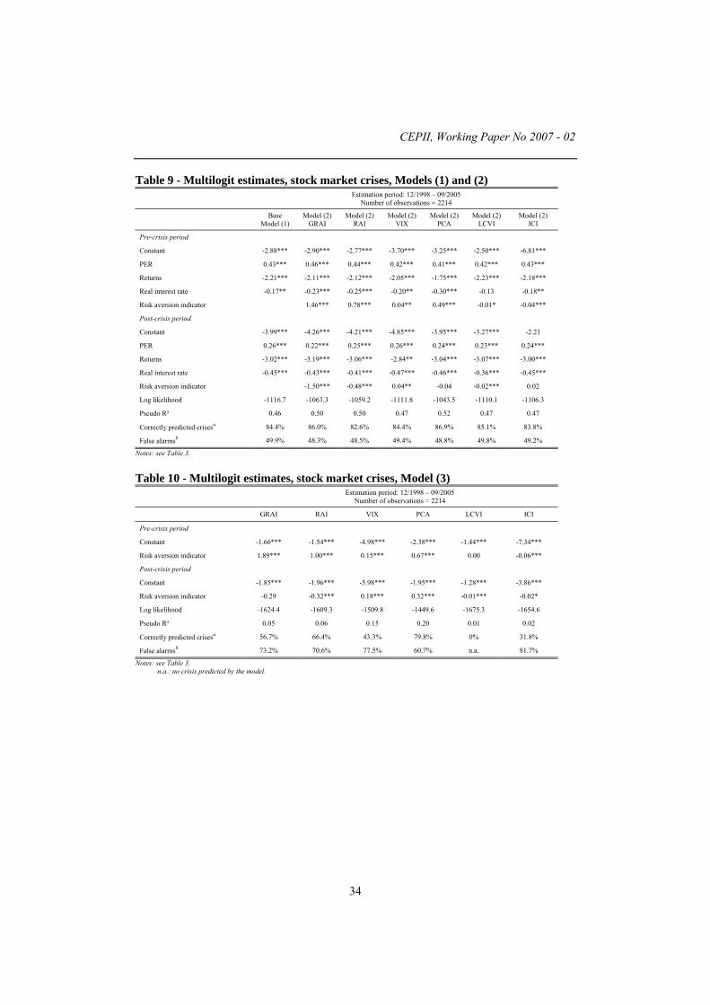
CEPII, Working Paper No 2007 - 02
34
Table 9 - Multilogit estimates, stock market crises, Models (1) and (2)Estimation period: 12/1998 – 09/2005
Number of observations = 2214
BaseModel (1)
Model (2)GRAI
Model (2)RAI
Model (2)VIX
Model (2)PCA
Model (2)LCVI
Model (2)ICI
Pre-crisis period
Constant -2.88*** -2.90*** -2.77*** -3.70*** -3.25*** -2.50*** -6.81***
PER 0.43*** 0.46*** 0.44*** 0.42*** 0.41*** 0.42*** 0.43***
Returns -2.21*** -2.11*** -2.12*** -2.05*** -1.75*** -2.23*** -2.18***
Real interest rate -0.17** -0.23*** -0.25*** -0.20** -0.30*** -0.13 -0.18**
Risk aversion indicator 1.46*** 0.78*** 0.04** 0.49*** -0.01* -0.04***
Post-crisis period
Constant -3.99*** -4.26*** -4.21*** -4.85*** -3.95*** -3.27*** -2.21
PER 0.26*** 0.22*** 0.25*** 0.26*** 0.24*** 0.23*** 0.24***
Returns -3.02*** -3.19*** -3.06*** -2.84** -3.04*** -3.07*** -3.00***
Real interest rate -0.45*** -0.43*** -0.41*** -0.47*** -0.46*** -0.36*** -0.45***
Risk aversion indicator -1.50*** -0.48*** 0.04** -0.04 -0.02*** 0.02
Log likelihood -1116.7 -1063.3 -1059.2 -1111.8 -1043.5 -1110.1 -1106.3
Pseudo R² 0.46 0.50 0.50 0.47 0.52 0.47 0.47
Correctly predicted crisesa 84.4% 86.0% 82.6% 84.4% 86.9% 85.1% 83.8%
False alarmsb 49.9% 48.3% 48.5% 49.4% 48.8% 49.8% 49.2%
Notes: see Table 3.
Table 10 - Multilogit estimates, stock market crises, Model (3)Estimation period: 12/1998 – 09/2005
Number of observations = 2214
GRAI RAI VIX PCA LCVI ICI
Pre-crisis period
Constant -1.66*** -1.54*** -4.98*** -2.38*** -1.44*** -7.34***
Risk aversion indicator 1.89*** 1.00*** 0.15*** 0.67*** 0.00 -0.06***
Post-crisis period
Constant -1.85*** -1.96*** -5.98*** -1.95*** -1.28*** -3.86***
Risk aversion indicator -0.29 -0.32*** 0.18*** 0.32*** -0.01*** -0.02*
Log likelihood -1624.4 -1609.3 -1509.8 -1449.6 -1675.3 -1654.6
Pseudo R² 0.05 0.06 0.15 0.20 0.01 0.02
Correctly predicted crisesa 56.7% 66.4% 43.3% 79.8% 0% 31.8%
False alarmsb 73.2% 70.6% 77.5% 60.7% n.a. 81.7%
Notes: see Table 3.n.a.: no crisis predicted by the model.
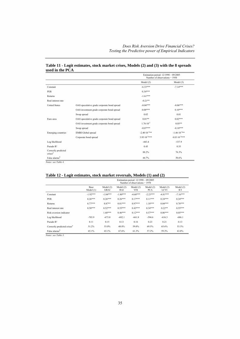
Does Risk Aversion Drive Financial Crises?Testing the Predictive power of Empirical Indicators
35
Table 11 - Logit estimates, stock market crises, Models (2) and (3) with the 8 spreadsused in the PCA
Estimation period: 12/1998 – 09/2005Number of observations = 1950
Model (2) Model (3)
Constant -6.33*** -7.14***
PER 0.34***
Returns -1.61***
Real interest rate -0.21**
United States OAS speculative grade corporate bond spread -0.04*** -0.06***
OAS investment grade corporate bond spread 0.08*** 0.10***
Swap spread 0.02 0.01
Euro area OAS speculative grade corporate bond spread 0.01** 0.02***
OAS investment grade corporate bond spread 1.76·10-3 0.05**
Swap spread -0.07*** -0.10***
Emerging countries EMBI Global spread -2.40·10-3** -1.46·10-3**
Corporate bond spread 3.95·10-3*** 4.83·10-3***
Log likelihood -443.4 -537.9
Pseudo R² 0.45 0.35
Correctly predictedcrisesa 88.2% 76.3%
False alarmsb 44.7% 50.6%
Notes: see Table 4.
Table 12 - Logit estimates, stock market reversals, Models (1) and (2)Estimation period: 12/1998 – 09/2005
Number of observations = 1970
BaseModel (1)
Model (2)GRAI
Model (2)RAI
Model (2)VIX
Model (2)PCA
Model (2)LCVI
Model (2)ICI
Constant -1.92*** -1.84*** -1.80*** -4.60*** -2.23*** -4.81*** -7.16***
PER 0.26*** 0.26*** 0.26*** 0.17*** 0.11*** 0.24*** 0.24***
Returns 0.77*** 0.87** 0.81*** 0.97*** 1.18*** 0.84*** 0.78***
Real interest rate 0.58*** 0.52*** 0.55*** 0.43*** 0.34*** 0.22** 0.55***
Risk aversion indicator 1.68*** 0.46*** 0.12*** 0.57*** 0.06*** 0.05***
Log likelihood -703.9 -673.0 -692.1 -661.8 -594.6 -616.3 -686.1
Pseudo R² 0.11 0.15 0.13 0.16 0.23 0.21 0.13
Correctly predicted crisesa 51.2% 53.0% 48.8% 59.0% 69.5% 65.6% 53.3%
False alarmsb 65.1% 65.1% 67.6% 61.3% 57.2% 59.3% 63.8%
Notes: see Table 3.
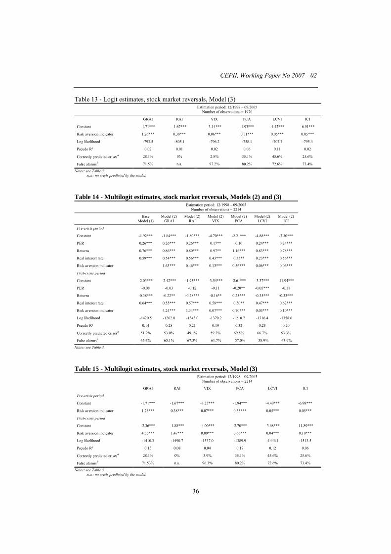
CEPII, Working Paper No 2007 - 02
36
Table 13 - Logit estimates, stock market reversals, Model (3)Estimation period: 12/1998 – 09/2005
Number of observations = 1970
GRAI RAI VIX PCA LCVI ICI
Constant -1.71*** -1.67*** -3.14*** -1.93*** -4.42*** -6.91***
Risk aversion indicator 1.26*** 0.38*** 0.06*** 0.31*** 0.05*** 0.05***
Log likelihood -793.5 -805.1 -796.2 -758.1 -707.7 -795.4
Pseudo R² 0.02 0.01 0.02 0.06 0.11 0.02
Correctly predicted crisesa 28.1% 0% 2.8% 35.1% 45.6% 25.6%
False alarmsb 71.5% n.a. 97.2% 80.2% 72.6% 73.4%
Notes: see Table 3.n.a.: no crisis predicted by the model.
Table 14 - Multilogit estimates, stock market reversals, Models (2) and (3)Estimation period: 12/1998 – 09/2005
Number of observations = 2214
BaseModel (1)
Model (2)GRAI
Model (2)RAI
Model (2)VIX
Model (2)PCA
Model (2)LCVI
Model (2)ICI
Pre-crisis period
Constant -1.92*** -1.84*** -1.80*** -4.70*** -2.21*** -4.88*** -7.30***
PER 0.26*** 0.26*** 0.26*** 0.17** 0.10 0.24*** 0.24***
Returns 0.76*** 0.86*** 0.80*** 0.97** 1.16*** 0.83*** 0.78***
Real interest rate 0.59*** 0.54*** 0.56*** 0.43*** 0.35** 0.23*** 0.56***
Risk aversion indicator 1.63*** 0.46*** 0.13*** 0.56*** 0.06*** 0.06***
Post-crisis period
Constant -2.03*** -2.42*** -1.95*** -3.54*** -2.61*** -3.37*** -11.94***
PER -0.08 -0.03 -0.12 -0.11 -0.20** -0.05*** -0.11
Returns -0.38*** -0.22** -0.28*** -0.16** 0.25*** -0.35*** -0.33***
Real interest rate 0.64*** 0.55*** 0.57*** 0.58*** 0.50** 0.47*** 0.62***
Risk aversion indicator 4.24*** 1.34*** 0.07*** 0.70*** 0.03*** 0.10***
Log likelihood -1420.5 -1262.0 -1343.0 -1370.2 -1210.7 -1316.4 -1358.6
Pseudo R² 0.14 0.28 0.21 0.19 0.32 0.23 0.20
Correctly predicted crisesa 51.2% 53.0% 49.1% 59.3% 69.5% 66.7% 53.3%
False alarmsb 65.4% 65.1% 67.3% 61.7% 57.0% 58.9% 63.9%
Notes: see Table 3.
Table 15 - Multilogit estimates, stock market reversals, Model (3)Estimation period: 12/1998 – 09/2005
Number of observations = 2214
GRAI RAI VIX PCA LCVI ICI
Pre-crisis period
Constant -1.71*** -1.67*** -3.27*** -1.94*** -4.49*** -6.98***
Risk aversion indicator 1.25*** 0.38*** 0.07*** 0.33*** 0.05*** 0.05***
Post-crisis period
Constant -2.36*** -1.88*** -4.00*** -2.70*** -3.68*** -11.89***
Risk aversion indicator 4.35*** 1.47*** 0.09*** 0.66*** 0.04*** 0.10***
Log likelihood -1410.3 -1490.7 -1537.0 -1389.9 -1446.1 -1513.5
Pseudo R² 0.15 0.08 0.04 0.17 0.12 0.06
Correctly predicted crisesa 28.1% 0% 3.9% 35.1% 45.6% 25.6%
False alarmsb 71.53% n.a. 96.3% 80.2% 72.6% 73.4%
Notes: see Table 3.n.a.: no crisis predicted by the model.

Does Risk Aversion Drive Financial Crises?Testing the Predictive power of Empirical Indicators
37
APPENDIX 1: THE DATABASE
The GRAI
The currency GRAI comprises 12 to 15 currencies quoted against the dollar according tothe periods for which the data are available: the Norwegian krone, the Czech koruna, theSwedish krona, the Deutsche Mark then the euro from 1999, the Australian dollar, theCanadian dollar, the Hong Kong dollar, the Singapore dollar, the New Zealand dollar, theSwiss franc, pound sterling, the Mexican peso, the South African rand, the yen and thePolish zloty.
The currency RAI is made up of 12 currencies over the whole period as a different numberof series over time would produce abrupt changes in the regression coefficient, whichwould distort the calculation.
The stock market GRAI and RAI include the major stock market indices of 27 developedand emerging economies: Argentina, Australia, Austria, Belgium, Brazil, Canada,Denmark, Finland, France, Germany, Greece, Hong Kong, Indonesia, Ireland, Italy, Japan,Malaysia, Netherlands, Norway, New Zealand, Portugal, South Africa, Spain, Sweden,Turkey, the United Kingdom and the United States.
Components of the PCA
Eight risk premia are used in the PCA. The data are taken from Bloomberg:
4 OAS corporate bond spreads for the euro area and the United States:7 for each
area, one spread for investment grade and another for speculative grade. Thesespreads are calculated by Merrill Lynch;
2 spreads for emerging markets: first, the EMBI Global,8 representing the risk
premium on their dollar-denominated external sovereign debt, calculated sincemid-1998 by J.P. Morgan on a large panel of emerging market countries; andsecond, an index of corporate debt, denominated in dollars or euro and issuedabroad, of a large number of emerging market countries. This index is calculatedby the bank Merrill Lynch and satisfies certain liquidity conditions;
2 swap spreads, one for the euro area and one for the United States.
7 For this, we use bonds that have an optional component – the option adjusted duration – to calculate the
credit spread between two bonds with the same maturity (Lubochinsky, 2002).8 The Emerging Markets Bond Index Global (EMBI Global) is an index that represents the average price of
bonds in emerging market countries.

CEPII, Working Paper No 2007 - 02
38
Crisis indicators
Currency crisis
The countries selected are the following: Argentina, Brazil, Bulgaria, Chile, Colombia,Czech Republic, Estonia, Hungary, Indonesia, Latvia, Lithuania, Mexico, Philippines,Poland, Romania, Singapore, South Korea, Thailand, Uruguay and Venezuela.
The sample period is from March 1995 to September 2005.
The data were taken from the IMF’s International Financial Statistics (IFS) database for the1995-2005 period as monthly data (quarterly data were made monthly by means of linearinterpolation): total reserves minus gold, line 1 l.d; money, line 34, quasi-money, line 35, toobtain the reserves/M2 ratio; real exchange rate, line ae, consumer prices, line 64, tocalculate the real exchange rate; and money market rate, lines 60, 60b or 60a (depending onthe availability of data and in this order of preference), to calculate the real interest rate(with the aid of consumer prices).
Stock market crisis
The countries selected are the following: Argentina, Australia, Austria, Belgium, Brazil,Canada, Denmark, Finland, France, Germany, Greece, Hong Kong, Indonesia, Ireland,Italy, Japan, Malaysia, Netherlands, Norway, New Zealand, Portugal, South Africa, Spain,Sweden, Turkey, the United Kingdom, and the United States.
The estimation period is from December 1995 to September 2005.
The indices, taken from Bloomberg, are the following: DAX (Germany), S&P/TSXComposite (Canada), DJIA (United States), CAC 40 (France), OMX Stockholm 30(Sweden), AEX (Pays-Bas), BEL20 (Belgium), MIB30 (Italia), Nikkei (Japan), FTSE 100(United Kingdom), IBEX 35 (Spain), PSI General (Portugal), OMX Copenhagen 20(Denmark), OMX Helsinki (Finland), ATX (Austria), Irish overall (Ireland), OBX(Norway), ASE General (Greece), ISE National 100 (Turkey), Johannesburg StockExchange (South Africa), S&P/ASX 200 (Australia), NZX Top 10 (New Zealand), HangSeng (Hong Kong), Kuala Lumpur Composite (Malaysia), Jakarta Composite (Indonesia),MERVAL (Argentina), BOVESPA Stock (Brazil). The returns have been calculated usingthese indices. The PER on these indices have also been obtained from Bloomberg. Interestrates have been taken from the IMF’s IFS database and calculated in the same way as forcurrency crises.

Does Risk Aversion Drive Financial Crises?Testing the Predictive power of Empirical Indicators
39
APPENDIX 2: RISK AVERSION INDICATORS GRAPHS
GRAI calculated on the foreign exchange market
1995 1996 1997 1998 1999 2000 2001 2002 2003 2004 2005-0.75
-0.50
-0.25
0.00
0.25
0.50
0.75
GRAI calculated on the stock market
1995 1996 1997 1998 1999 2000 2001 2002 2003 2004 2005-0.75
-0.50
-0.25
0.00
0.25
0.50
0.75
RAI calculated on the foreign exchange market
1995 1996 1997 1998 1999 2000 2001 2002 2003 2004 2005-2.4
-1.6
-0.8
-0.0
0.8
1.6
2.4
RAI calculated on the stock market
1995 1996 1997 1998 1999 2000 2001 2002 2003 2004 2005-2.4
-1.6
-0.8
-0.0
0.8
1.6
2.4
Risk aversion indicator measuredby the first component of the PCA
1999 2000 2001 2002 2003 2004 2005-4
-3
-2
-1
0
1
2
3
4
5
VIX
1995 1996 1997 1998 1999 2000 2001 2002 2003 2004 200510
15
20
25
30
35
40
45
LCVI
1998 1999 2000 2001 2002 2003 2004 200510
20
30
40
50
60
70
80
90
100
ICI
1998 1999 2000 2001 2002 2003 2004 2005-115
-110
-105
-100
-95
-90
-85
-80
Note: vertical columns: Asian crisis (07/1997 – 12/1997), Russian crisis and failure of LTCM (08/1998 – 09/1998) and downtrend on the main stockmarkets (09/2000 – 09/2002). Vertical line: terrorist attacks September, 11th, 2001.

CEPII, Working Paper No 2007 - 02
40
APPENDIX 3: CURRENCY AND STOCK MARKET CRISES
1. Identification of crises
Estimation period: 07/1995 – 09/2005
Currency crises Stock market crises
Argentina January 2002 Argentina May 2002
Brazil January 1999 Australia September 2002
Bulgaria May 1996 Austria September 1998
Chilli Belgium September 2002
Colombia September 1998 Brazil July 2002
Czech Republic May 1997 et August 1998 Canada September 2001 and September 2002
Estonia June 2003 Denmark July 2002
Hungary Finland August 2001
Indonesia April 1997 France July 2002
Korea December 1997 Germany September 2002
Latvia Greece September 2001
Lithuania Hong Kong July 1998
Mexico Indonesia
Philippines September 1997 Ireland July 2002
Poland August 1998 and March 2005 Italy July 2002
Romania July 1996 and November 1999 Japan September 2001
Singapore December 1997 Malaysia January 1998
Thailand July 1997 Netherlands September 2002
Uruguay April 2002 New Zealand August 1998
Venezuela February 2002 Norway September 2002
Portugal September 2001 and September 2002
South Africa August 1998
Spain September 2001 and September 2002
Sweden June 2002
Turkey November 2000
United Kingdom July 2002
United States September 2001 and September 2002

Does Risk Aversion Drive Financial Crises?Testing the Predictive power of Empirical Indicators
41
Number of identified crises by year
Currency crises
1995 1996 1997 1998 1999 2000 2001 2002 2003 2004 20050
2
5
8
10
12
15
18
20
Stock market crises
1995 1996 1997 1998 1999 2000 2001 2002 2003 2004 20050
2
5
8
10
12
15
18
20

CEPII, Working Paper No 2007 - 02
42
Identification of currency crises: pressure index (full line) and crisis threshold (dotted line) for 4 selected countriesArgentina
1995 1996 1997 1998 1999 2000 2001 2002 2003 2004 2005-0.10
-0.05
0.00
0.05
0.10
0.15
0.20
0.25
0.30
0.35
Brazil
1995 1996 1997 1998 1999 2000 2001 2002 2003 2004 2005-0.15
-0.10
-0.05
0.00
0.05
0.10
0.15
0.20
0.25
Korea
1995 1996 1997 1998 1999 2000 2001 2002 2003 2004 2005-0.15
-0.10
-0.05
0.00
0.05
0.10
0.15
0.20
0.25
0.30
Thailand
1995 1996 1997 1998 1999 2000 2001 2002 2003 2004 2005-0.100
-0.075
-0.050
-0.025
-0.000
0.025
0.050
0.075
0.100
0.125
Note: vertical lines: identified crises. Vertical columns: pre-crisis periods.
Identification of stock market crises: CMAX (full line) and crisis threshold (dotted line) for 4 selected countries
Germany
1999 2000 2001 2002 2003 2004 20050.3
0.4
0.5
0.6
0.7
0.8
0.9
1.0
1.1
France
1999 2000 2001 2002 2003 2004 20050.4
0.5
0.6
0.7
0.8
0.9
1.0
1.1
United Kingdom
1999 2000 2001 2002 2003 2004 20050.5
0.6
0.7
0.8
0.9
1.0
1.1
United States
1999 2000 2001 2002 2003 2004 20050.65
0.70
0.75
0.80
0.85
0.90
0.95
1.00
1.05
Note: vertical lines: identified crises. Vertical columns: pre-crisis periods.Identification of stock market reversals: CMAX (full line) and crisis threshold (dotted line) for 4 selected countries

Does Risk Aversion Drive Financial Crises?Testing the Predictive power of Empirical Indicators
43
Germany
1999 2000 2001 2002 2003 2004 20050.3
0.4
0.5
0.6
0.7
0.8
0.9
1.0
1.1
France
1999 2000 2001 2002 2003 2004 20050.4
0.5
0.6
0.7
0.8
0.9
1.0
1.1
United Kingdom
1999 2000 2001 2002 2003 2004 20050.5
0.6
0.7
0.8
0.9
1.0
1.1
United States
1999 2000 2001 2002 2003 2004 20050.65
0.70
0.75
0.80
0.85
0.90
0.95
1.00
1.05
Note: vertical lines: identified reversals. Vertical columns: pre-crisis periods.

CEPII, Working Paper No 2007 - 02
44
2. Simulation with control variables
Currency crisis probabilities for 4 selected countriesLogit estimates, Model (1)
Argentina
1995 1996 1997 1998 1999 2000 2001 2002 2003 2004 20050.00
0.25
0.50
0.75
1.00
Cutoff = 0.20
Brazil
1995 1996 1997 1998 1999 2000 2001 2002 2003 2004 20050.00
0.25
0.50
0.75
1.00
Cutoff = 0.20
Korea
1995 1996 1997 1998 1999 2000 2001 2002 2003 2004 20050.00
0.25
0.50
0.75
1.00
Cutoff = 0.20
Thailand
1995 1996 1997 1998 1999 2000 2001 2002 2003 2004 20050.00
0.25
0.50
0.75
1.00
Cutoff = 0.20
Note: vertical lines: identified crises. Vertical columns: pre-crisis periods.
Stock market crisis probabilities for 4 selected countriesLogit estimates, Model (1)
Germany
1999 2000 2001 2002 2003 2004 20050.00
0.25
0.50
0.75
1.00
Cutoff = 0.20
France
1999 2000 2001 2002 2003 2004 20050.00
0.25
0.50
0.75
1.00
Cutoff = 0.20

Does Risk Aversion Drive Financial Crises?Testing the Predictive power of Empirical Indicators
45
United Kingdom
1999 2000 2001 2002 2003 2004 20050.00
0.25
0.50
0.75
1.00
Cutoff = 0.20
United States
1999 2000 2001 2002 2003 2004 20050.00
0.25
0.50
0.75
1.00
Cutoff = 0.20
Note: vertical lines: identified crises. Vertical columns: pre-crisis periods.
Stock market reversal probabilities for 4 selected countriesLogit estimates, Model (1)
Germany
1999 2000 2001 2002 2003 2004 20050.00
0.25
0.50
0.75
1.00
Cutoff = 0.20
France
1999 2000 2001 2002 2003 2004 20050.00
0.25
0.50
0.75
1.00
Cutoff = 0.20
United Kingdom
1999 2000 2001 2002 2003 2004 20050.00
0.25
0.50
0.75
1.00
Cutoff = 0.20
United States
1999 2000 2001 2002 2003 2004 20050.00
0.25
0.50
0.75
1.00
Cutoff = 0.20
Note: vertical lines: identified reversals. Vertical columns: pre-crisis periods.

CEPII, Working Paper No 2007 - 02
46
List of working papers released by CEPII9
No Title Authors
2007-01
World Growth and International Capital Flows in theXXIst Century: A prospective analysis with theINGENUE 2 model
10
M. Aglietta, V. BorgyJ. Château, M. Juillard
J. le Cacheux,G. Le Garrec &.
V. Touzé
2006-27 Current Account Reversals and Long TermImbalances : Application to the Central and EasternEuropean Countries
K. Benhima & O.Havrylchyk
2006-26 Do Legal Origins and Brankruptcy Laws : theEuropean Experience (1808-1914)
J. Sgard
2006-25 Taux d’intérêt et marchés boursiers : une analyseempirique de l’intégration financière internationale
V. Borgy & V. Mignon
2006-24 On Legal Origins & Bankruptcy Laws : the EuropeanExperience (1808-1914)
J. Sgard
2006-23 Market Access Impact on Individual Wage: Evidencefrom China
L. Hering & S. Poncet
2006-22 FDI in Chinese Cities: Spillovers and Impact onGrowth
N. Madariaga& S. Poncet
2006-21 Are Financial Distortions an Impediment to EconomicGrowth? Evidence from China
A. Guariglia& S. Poncet
2006-20 World Consistent Equilibrium Exchange Rates A. Bénassy-Quéré,A. Lahrèche-Révil
& V. Mignon
2006-19 Institutions and Bilateral Asset Holdings V. Salins& A. Bénassy-Quéré
2006-18 Vertical Production Networks: Evidence from France M. Fouquin,L. Nayman
9 Working papers are circulated free of charge as far as stocks are available; thank you to send your request
to CEPII, Sylvie Hurion, 9, rue Georges-Pitard, 75015 Paris, or by fax : (33) 01 53 68 55 04 or by e-mailsylvie.hurion @ cepii.fr. Also available on: \\www.cepii.fr. Working papers with * are out of print. Theycan nevertheless be consulted and downloaded from this website.9 Les documents de travail sont diffusés gratuitement sur demande dans la mesure des stocks disponibles.
Merci d’adresser votre demande au CEPII, Sylvie Hurion, 9, rue Georges-Pitard, 75015 Paris, ou parfax : (33) 01 53 68 55 04 ou par e-mail sylvie.hurion @ cepii.fr. Egalement disponibles sur : \\www.cepii.fr.Les documents de travail comportant * sont épuisés. Ils sont toutefois consultable sur le web CEPII.10
We thank Agnès Benassy-Quéré for her valuable remarks and suggestions on a previous version of thepaper.
Does Risk Aversion Drive Financial Crises?Testing the Predictive power of Empirical Indicators
47
& L. Wagner
2006-17 Import Prices, Variety and the Extensive Margin ofTrade
G. Gaulier& I. Méjean
2006-16 The Long Term Growth Prospects of the WorldEconomy: Horizon 2050
S. Poncet
2006-15 Economic Integration in Asia: Bilateral Free TradeAgreements Versus Asian Single Market
M. H. Bchir& M. Fouquin
2006-14 Foreign Direct Investment in China: Reward orRemedy?
O. Havrylchyk& S. Poncet
2006-13 Short-Term Fiscal Spillovers in a Monetary Union A. Bénassy-Quéré
2006-12 Can Firms’ Location Decisions Counteract theBalassa-Samuelson Effect?
I. Méjean
2006-11 Who’s Afraid of Tax Competition? Harmless TaxCompetition from the New European Member States
A. Lahrèche-Révil
2006-10 A Quantitative Assessment of the Outcome of theDoha Development Agenda
Y. Decreux& L. Fontagné
2006-09 Disparities in Pension Financing in Europe: Economicand Financial Consequences
J. Château& X. Chojnicki
2006-08 Base de données CHELEM-BAL du CEPII H. Boumellassa& D. Ünal-Kesenci
2006-07 Deindustrialisation and the Fear of Relocations in theIndustry
H. Boulhol& L. Fontagné
2006-06 A Dynamic Perspective for the Reform of the Stabilityand Gowth Pact
C. Deubner
2006-05 China’s Emergence and the Reorganisation of TradeFlows in Asia
G. Gaulier, F. Lemoine& D. Ünal-Kesenci
2006-04 Who Pays China's Bank Restructuring Bill? G. Ma
2006-03 Structural Determinants of the Exchange-Rate Pass-Through
G. Gaulier,A. Lahrèche-Révil
& I. Méjean
2006-02 Exchange-Rate Pass-Through at the Product Level G. Gaulier,A. Lahrèche-Révil
& I. Méjean
2006-01 Je t'aime, moi non plus : Bilateral Opinions andInternational Trade
A.C. Disdier& T. Mayer
2005-23 World Trade Competitiveness: A DisaggregatedView by Shift-Share Analysis
A. Cheptea, G. Gaulier& S. Zignago
2005-22 Chômage et réformes du marché du travail au Japon E. Dourille-Feer

CEPII, Working Paper No 2007 - 02
48
2005-21 Profitability of Foreign and Domestic Banks inCentral and Eastern Europe: Does the Mode of EntryMatter?
O. Havrylchyk &E. Jurzyk
2005-20 ECB Governance in an Enlarged Eurozone A. Bénassy-Quéré &E. Turkisch
2005-19 What Are EU Trade Preferences Worth for Sub-Saharan Africa and Other Developing Countries?
F. Candau & S. Jean
2005-18 Binding Overhang and Tariff-Cutting Formulas M.H. Bchir, S. Jean &D. Laborde
2005-17 International Trade and Income Distribution:Reconsidering the Evidence
I. Bensidoun, S. Jean &A. Sztulman
2005-16 China and the Relationship between the Oil Price andthe Dollar
A. Bénassy-Quéré,V. Mignon & A. Penot
2005-15 Consequences of Alternative Formulas forAgricultural Tariff Cuts
S. Jean, D. Laborde &W. Martin
2005-14 Is Erosion of Tariff Preferences a Serious Concern? A. Bouët, L. Fontagné& S. Jean
2005-13 The Consequences of Agricultural TradeLiberalization for Developing Countries:Distinguishing Between Genuine Benefits and FalseHopes
J.C. Bureau, S. JeanA. Matthews
2005-12 From Bound Duties to Actual Protection: IndustrialLiberalisation in the Doha Round
M.H. Bchir,L. Fontagné & S. Jean
2005-11 Impact de l'ouverture financière sur les inégalitésinternes dans les pays émergents
A. Bénassy-Quéré &V. Salins
2005-10 Disentangling Horizontal and Vertical Intra-IndustryTrade
L. Fontagné,M. Freudenberg &
G. Gaulier
2005-09 China's Integration in East Asia: Production Sharing,FDI & High-Tech Trade
G. Gaulier, F. LemoineD. Ünal-Kesenci
2005-08 Tax Competition and Public Input A. Bénassy-Quéré,N. Gobalraja &
A. Trannoy
2005-07 Trade Liberalisation, Growth and Poverty in Senegal:A Dynamic Microsimulation CGE Model Analysis
N. Annabi, F. Cissé,J. Cockburn &
B. Decaluwé
2005-06 Migration, Trade and Wages A. Hijzen & P. Wright
2005-05 Institutional Determinants of Foreign Investment A. Bénassy-Quéré,M. Coupet & T. Mayer

Does Risk Aversion Drive Financial Crises?Testing the Predictive power of Empirical Indicators
49
2005-04 L’économie indienne : changements structurels etperspectives à long terme
S. Chauvin &F. Lemoine
2005-03 Programme de travail du CEPII pour 2005
2005-02 Market Access in Global and Regional Trade T. Mayer& S. Zignago
2005-01 Real Equilibrium Exchange Rate in China V. Coudert &C. Couharde
2004-22 A Consistent, ad-valorem Equivalent Measure ofApplied Protection Across the World: The MAcMap-HS6 Database
A. Bouët, Y. Decreux,L. Fontagné, S. Jean
& D. Laborde
2004-21 IMF in Theory: Sovereign Debts, Judicialisation andMultilateralism
J. Sgard
2004-20 The Impact of Multilateral Liberalisation on EuropeanRegions: a CGE Assessment
S. Jean & D. Laborde
2004-19 La compétitivité de l'agriculture et des industriesagroalimentaires dans le Mercosur et l'Unioneuropéenne dans une perspective de libéralisationcommerciale
N. Mulder, A. Vialou,B. David,
M. Rodriguez &M. Castilho
2004-18 Multilateral Agricultural Trade Liberalization: TheContrasting Fortunes of Developing Countries in theDoha Round
A. Bouët, J.C. Bureau,Y. Decreux & S. Jean
2004-17 UK in or UK out? A Common Cycle Analysisbetween the UK and the Euro Zone
J. Garnier
2004-16 Regionalism and the Regionalisation of InternationalTrade
G. Gaulier, S. Jean &D. Ünal-Kesenci
2004-15 The Stock-Flow Approach to the Real Exchange Rateof CEE Transition Economies
B. Egert,A. Lahrècche-Révil &
K. Lommatzsch
2004-14 Vieillissement démographique, épargne et retraite :une analyse à l’aide d’un modèle d’équilibre général àagents hétérogènes
C. Bac & J. Chateau
2004-13 Burden Sharing and Exchange-Rate Misalignmentswithin the Group of Twenty
A. Bénassy-Quéré,P. Duran-Vigneron,
A. Lahrèche-Révil &V. Mignon
2004-12 Regulation and Wage Premia S. Jean & G. Nicoletti
2004-11 The Efficiency of Fiscal Policies: a Survey of theLiterature
S. Capet
2004-10 La réforme du marché du travail en Allemagne : les S. Capet

CEPII, Working Paper No 2007 - 02
50
enseignements d’une maquette
2004-09 Typologie et équivalence des systèmes de retraites P. Villa
2004-08 South – South Trade: Geography Matters S. Coulibaly &L. Fontagné
2004-07 Current Accounts Dynamics in New EU Members:Sustainability and Policy Issues
P. Zanghieri
2004-06 Incertitude radicale et choix du modèle P. Villa
2004-05 Does Exchange Rate Regime Explain Differences inEconomic Results for Asian Countries?
V. Coudert & M. Dubert
2004-04 Trade in the Triad: How Easy is the Access to LargeMarkets?
L. Fontagné, T. Mayer& S. Zignago
2004-03 Programme de travail du CEPII pour 2004
2004-02 Technology Differences, Institutions and EconomicGrowth: a Conditional Conditional Convergence
H. Boulhol
2004-01 Croissance et régimes d’investissement P. Villa

Working paper No 2007- 02
CEPIIDOCUMENTS DE TRAVAIL / WORKING PAPERS
Si vous souhaitez recevoir des Documents de travail,merci de remplir le coupon-réponse ci-joint et de le retourner à :
Should you wish to receive copies of the CEPII’s Working papers,just fill the reply card and return it to:
Sylvie HURION – PublicationsCEPII – 9, rue Georges-Pitard – 75740 Paris – Fax : (33) 1.53.68.55.04
M./Mme / Mr./Mrs ..................................................................................................................
Nom-Prénom / Name-First name .............................................................................................
Titre / Title ...............................................................................................................................
Service / Department................................................................................................................
Organisme / Organisation ........................................................................................................
Adresse / Address.....................................................................................................................
Ville & CP / City & post code..................................................................................................Pays / Country.............................................................. Tél......................................................Your e-mail ..............................................................................................................................
Désire recevoir les Document de travail du CEPII n° :
Wish to receive the CEPII’s Working Papers No:..................................................................
..................................................................................................................................................
..................................................................................................................................................
..................................................................................................................................................
..................................................................................................................................................
..................................................................................................................................................
..................................................................................................................................................
..................................................................................................................................................
..................................................................................................................................................
Souhaite être placé sur la liste de diffusion permanente (pour les bibliothèques)Wish to be placed on the standing mailing list (for Libraries).

Titre
52