NBER WORKING PAPER SERIES

DOES THE EFFECT OF POLLUTION ON INFANT MORTALITY DIFFER BETWEENDEVELOPING AND DEVELOPED COUNTRIES? EVIDENCE FROM MEXICO

CITY

Eva O. Arceo-GomezRema HannaPaulina Oliva

Working Paper 18349http://www.nber.org/papers/w18349

NATIONAL BUREAU OF ECONOMIC RESEARCH1050 Massachusetts Avenue

Cambridge, MA 02138August 2012

We thank Jon Hill and Katherine Kimble for excellent research assistance. We are grateful to DavidCard, Janet Currie, Olivier Deschenes, Heather Royer, Heidi Williams, Catherine Wolfram and LucasDavis for helpful comments, as well as seminar participants at CEPR Development Meetings Pre-Conference,the ARE Berkeley Seminar, the Environment and Human Capital Conference, and the UC Santa BarbaraLabor Lunch. We especially thank Marta Vicarelli for providing us with the temperature data. Thisproject was funded in part by the Harvard Center for Population and Development Studies and UCMexus.The views expressed herein are those of the authors and do not necessarily reflect the views of theNational Bureau of Economic Research.

NBER working papers are circulated for discussion and comment purposes. They have not been peer-reviewed or been subject to the review by the NBER Board of Directors that accompanies officialNBER publications.

© 2012 by Eva O. Arceo-Gomez, Rema Hanna, and Paulina Oliva. All rights reserved. Short sectionsof text, not to exceed two paragraphs, may be quoted without explicit permission provided that fullcredit, including © notice, is given to the source.

Does the Effect of Pollution on Infant Mortality Differ Between Developing and DevelopedCountries? Evidence from Mexico CityEva O. Arceo-Gomez, Rema Hanna, and Paulina OlivaNBER Working Paper No. 18349August 2012JEL No. O1,Q53

ABSTRACT

Much of what we know about the marginal effect of pollution on infant mortality is derived from developedcountry data. However, given the lower levels of air pollution in developed countries, these estimatesmay not be externally valid to the developing country context if there is a nonlinear dose relationshipbetween pollution and mortality or if the costs of avoidance behavior differs considerably betweenthe two contexts. In this paper, we estimate the relationship between pollution and infant mortalityusing data from Mexico. We find that an increase of 1 parts per billion in carbon monoxide (CO) overthe last week results in 0.0032 deaths per 100,000 births, while a 1 �g/m3 increase in particulate matter(PM10) results in 0.24 infant deaths per 100,000 births. Our estimates for PM10 tend to be similar(or even smaller) than the U.S. estimates, while our findings on CO tend to be larger than those derivedfrom the U.S. context. We provide suggestive evidence that a non-linearity in the relationship betweenCO and health explains this difference.

Eva O. Arceo-GomezCIDE – División de EconomíaCarretera México-Toluca 3655, Lomas de Santa FeMéxico, D.F. 01210eva.arceo@cide.edu

Rema HannaKennedy School of GovernmentHarvard University79 JFK StreetCambridge, MA 02138and NBERRema_Hanna@hks.harvard.edu

Paulina Oliva Department of Economics 2127 North Hall University of California Santa Barbara, CA 93106 and NBER oliva@econ.ucsb.edu

1  

I. INTRODUCTION

Pollution is a grave concern in much of the developing world, with levels that are often orders of

magnitude higher than in developed countries. Using comparable data, Greenstone and Hanna

(2011) document air pollution levels that are five to seven times higher in India and China than

in the United States. This may translate into many lost lives: The OECD estimates that almost

1.5 million individuals die from exposure to particulates each year, many more than who die

from malaria or unclean water. With pollution levels predicted to rise, the OECD claims that this

figure may exceed 3.5 million people per year by 2050, with most of these deaths occurring in

rapidly industrializing countries, such as India and China (OECD Outlook, 2011).

Much of what we know about the causal relationship between pollution and infant health

comes from developed country settings (for example, see Greenstone and Chay, 2003; Currie

and Neidell, 2005).1 However, there are two important reasons why these estimates may have

limited external validity to the developing country context. First, they may be limited if there is

a non-linear dose-response relationship between pollution and infant mortality. If we expect, for

example, that marginal changes in pollution are more damaging at higher levels of air pollution,

using developed country estimates would cause us to grossly underestimate the effect in many

developing countries. However, if there is an inflection point through which pollution needs to

fall beneath before health gains can be realized, using developed country estimates could

alternatively lead us to overestimate the effect. Similarly, due to a host of factors (i.e. disease

environments, access to health care), infant mortality rates are significantly higher in many

developing countries. As such, it is possible that pollution may exert a larger effect on infants if

they are already weakened by these other factors, or alternatively, it is possible that a marginal

increase in pollution may be negligible if these other factors supersede the pollution effect.

Second, the effect of pollution on health may be highly dependent on behavior (for

example, see Neidell and Moretti, 2011; Graff Zivin and Neidell, 2009; Deschenes, Greenstone

and Shapiro, 2012). Avoidance behavior may be costlier in the developing world, given less

access to health care and lower quality housing stock, which would imply that a marginal

decrease in pollution may have a larger overall health impact in the developing world. However,

                                                            1 Exceptions include Jayachandran (2006), who explores the impact of smoke from forest fires in Indonesia on infant health; Greenstone and Hanna (2011) who estimate the effect of mandated catalytic converters on infant mortality rates in India, but have a noisy estimate of the policy impact due to limited data; and Tanaka (2012), who measures the effect of more stringent environmental regulation in China.

2  

the effect could also be smaller if, for example, individuals have permanently adapted to bad

pollution by keeping infants indoors or wearing breathing masks regularly.2 Given these two

potential factors, applying estimates of the marginal effect of pollution that are derived from the

United States to developing countries may be highly misleading for policy. Furthermore, given

the theoretical ambiguity regarding the bias that these estimates would produce, it is difficult to

assess the direction in which we would be wrong.

The shortage of this type of analysis for developing countries stems from two main

challenges. First, data constraints tend to be more severe in developing countries. Quite

frequently, disaggregated data on infant births and deaths are not accurately recorded or

computerized. Even when the data are available, the validity of the data may be questionable as

there is substantial selection as to which births and deaths are registered. Moreover, there are

fewer stations systematically measuring pollution levels in developing countries, and so there is

potentially less variation in pollution to exploit.

Second, there is a simultaneity problem in estimating the relationship between pollution

and health. This problem is typically addressed by one of two methods. First, one can use a

policy instrument to tease out exogenous variation in pollution. However, despite the fact that

environmental regulations in developing countries often look similar to those in the United

States, they are often riddled with implementation and enforcement problems that result in more

limited impacts, resulting in a weak first stage. For example, Greenstone and Hanna (2011)

experience this problem when using environmental regulations in India as an instrument for

pollution.3 The second methodology typically used is a fixed effects model that controls for

time-invariant differences across locations and overall trends (see, for example, Currie and

Neidell, 2005). This type of empirical model can be challenging when using data from the

developing world, as the measurement error that may arise from using sparser pollution data than

in the United States may be exacerbated by the inclusion of fixed effects.4

In this study, we aim to address these problems and estimate the impact of pollution on

infant mortality in a developing country context. To do so, we construct weekly, municipality-                                                            2 As higher pollution is more visible, avoidance behaviors may be more likely since the costs of learning about pollution levels may be lower. 3 One exception is Tanaka (2012), which studies the effect of more stringent regulation in China on infant mortality. 4 As Currie and Neidell (2005) discuss, measurement error has also been noted in the United States context as well. Schlenker and Reed (2011) and Knittel, Miller, and Sanders (2011) find larger impacts of pollution on health when using an instrumental variables strategy as compared to fixed effects methods using United States data, which both claim is consistent with classical measurement error being exacerbated with the fixed effects methodology.

3  

level measures of pollution and mortality for 48 municipalities across Mexico City between the

years 1997 to 2006. Mexico City is a highly relevant context in which to study this relationship.

On average, it experiences both the high levels of pollution and mortality that are common in

many developing countries. However, given the high variance in pollution levels, the range of

pollution also encompasses a range similar to that observed in the United States. These two facts

will allow us to estimate the marginal effect of pollution at a range that is typical for developing

countries, and then to compare this estimate to the marginal effect at the ranges used in the

previous estimates for the United States.

We first employ a fixed effects technique, controlling for time-invariant characteristics of

municipalities, week fixed effects, and municipality-specific year trends. Using this method, we

find no impact of pollution on mortality. However, despite access to very high quality pollution

measures, station coverage is sparse: depending on the pollutant and year, our pollution

measures are derived from between 10 to 26 stations. Given that fixed effects models are

particularly sensitive to classical measurement error, our estimates may be severely biased

downward.

Instead, we exploit the meteorological phenomenon of thermal inversions. An inversion

occurs when a mass of hot air gets caught above a mass of cold air, trapping pollutants.

Conditional on temperature, inversions themselves do not represent a health risk per se other

than the accumulation of pollutants. As such, we can use the number of inversions in a given

week to instrument for pollution levels that week. We find that each additional inversion leads

to a 3.5 percent increase in particulate matter measuring 10µm or less (PM10) and a 5.4 percent

increase in carbon monoxide (CO), conditional on municipality fixed effects, municipality-

specific time trends, polynomials in temperature and weather controls.

With the instrumental variables strategy, we find robust evidence of pollution on infant

mortality. Our estimates imply that 1 µg/m3 increase in 24-hour PM10 results in 0.24 infant

deaths per 100,000 births. Similarly, 1 ppb increase in the 8-hour maximum for CO results in

0.0032 per 100,000 births.5 We find no significant effect on neonatal deaths (children 28 days

and younger). As a test of the causal pathway, we then separate deaths into those that are likely

to be pollution related (i.e. respiratory and cardiovascular disease) versus those that are less

                                                            5 As we illustrate below, these results are robust to different definitions of mortality, different controls for seasonality, the inclusion of outliers and different weather and temperature controls.

4  

likely to be pollution related (i.e. digestive, congenital, accidents, homicides, etc.). We find

statistically and policy significant effects of pollution on both neonatal and infant deaths from

respiratory and cardiovascular disease. As we would expect if we had indeed isolated the effect

of pollution from other factors (i.e. income, health preferences), we find no effect of pollution on

deaths from other causes.

Finally, we compare our estimates to those derived in the United States setting.

Specifically, we compare our estimates to Currie and Neidell (2005) [CN], Knittel, Miller, and

Sanders (2011) [KMS], Chay and Greenstone (2003) [CG], and Currie, Neidell, and Schmieder

(2009) [CNS].6 We find larger marginal effects of CO on infant mortality than CN and CNS;

we also find larger point estimates that KMS, but they do not observe a significant effect of CO

on infant mortality. We provide suggestive evidence that this is driven by non-linearities in the

effect of CO: constraining the Mexico City pollution data to be within the range of CO values

observed in the United States results in estimates that are roughly the same magnitude as CN.

For PM10, our results are near identical to CG’s results, despite the fact that the mean level of

pollution in their setting is roughly half of that in Mexico City. This is consistent with the fact

that we do not observe a non-linear effect for PM10 within our sample.7

The paper proceeds as follows. In Section II, we describe our empirical methods and

data, while we provide our findings in Section III. Section IV provides a discussion of our

estimates with those from the United States context. Section V concludes.

II. EMPIRICAL METHOD, DATA, AND SUMMARY STATISTICS

In this section, we first discuss some of the existing empirical methods for estimating the

relationship between air pollution and infant mortality. We then detail our empirical strategy in

Section II.B. Finally, we describe the data that we collected for this project.

II.A. Existing Empirical Methodologies

Our objective is to estimate the relationship between pollution ( ) in a municipality (m) in a

given week (w) and mortality per 100,000 live births ( ), or the parameter :

                                                            6 Note that other papers in the US context explore the effect of pollution on child and infant health (for example, see Lleras-Muney, 2010). We only include papers that study comparable infant mortality outcomes. 7 Although as we discuss more in depth below, we are highly cautious about this result because we have problems of power in our first stage for PM10. Thus, we only take this evidence as very suggestive.

5  

Equation 1:

where captures all unobserved determinants of mortality. There are many reasons to believe

the identification assumption does not hold in this case. For example, areas with low levels of

pollution may be richer, and thus have lower levels of mortality regardless of pollution. One

method to solve the endogeneity problem would be to estimate a fixed effects model:

Equation 2:

where is a set of municipality fixed effects that control for permanent differences across

municipalities, such as time-invariant socioeconomic characteristics. Similarly, is a set of

week fixed effects, which controls for common factors (e.g. city-wide economic shocks) in a

given week that could affect both pollution levels and infant mortality. The fixed effects model

represents a substantial improvement over the standard cross-sectional regression. However, two

concerns remain. First, may still be subject to bias if there are unobservable, time-varying

differences across municipalities. One way to account for this is to include municipality-

specific, linear time trends. However, this may not capture sharp or non-monotonic changes in

omitted pollution and infant mortality determinants, such as road improvements that could result

in fewer traffic jams and faster access for emergency vehicles, or similarly, protests and

demonstrations that results in disrupted travel patterns. Second, classical measurement error in

the pollution variable will bias downwards. Fixed effects estimators exacerbate measurement

error, biasing further towards zero. As compared to developed country settings, this may be

particularly problematic in developing countries, where pollution-monitoring stations are sparse:

for example, as we discuss below, we exploit data from 10 to 26 stations.

II.B. Exploiting Thermal Inversions in an Instrumental Variables Framework

We consider an instrumental variables strategy, which will likely minimize bias from both

endogeneity and classical measurement error. Specifically, we exploit a meteorological

phenomenon: the existence of thermal inversions. Inversions are a common occurrence in many

cities around the world, ranging from Mumbai, Los Angeles, San Paulo, Salt Lake City,

Santiago, Vancouver, Prague, etc.8 Air temperature in the troposphere usually falls with altitude

at about 6.5 degrees Celsius per 1,000 meters. However, sometimes there is a mass of hot air on

                                                            8 The great smog of 1952 in the UK was caused by an inversion episode and was blamed for upwards of 12,000 deaths (Bell and Davis, 2001). This incident sparked greater interest in environmental regulation in the UK.

6  

top of a mass of cold air; this is called a thermal inversion. There are typically three reasons why

this can occur: First, radiation inversions are generated in clear nights when the ground and the

air in touch with the ground are cooled faster than higher air layers. The conditions for radiation

inversions are more frequent in the winter: under clear conditions, the earth's infrared emissions

warm the higher layers of air. The cold ground temperatures cool causing the air that is close to

the ground to remain at a lower temperature than the air above. Second, inversions by subsidence

occur from vertical air movements when a layer of cold air descends between a layer of hot air.

Third, inversions can also be produced when layers of air at different temperatures move

horizontally and a layer of cold air develops below a layer of hot air (Jacobson, 2002).

The thermal inversion does not represent a health risk in itself, but when it occurs in

conjunction with high levels of vehicle and industrial emissions, it may result in the temporary

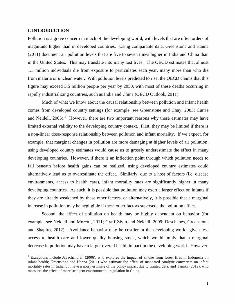
accumulation of pollutants.9 Specifically, when emissions are released in the atmosphere, they

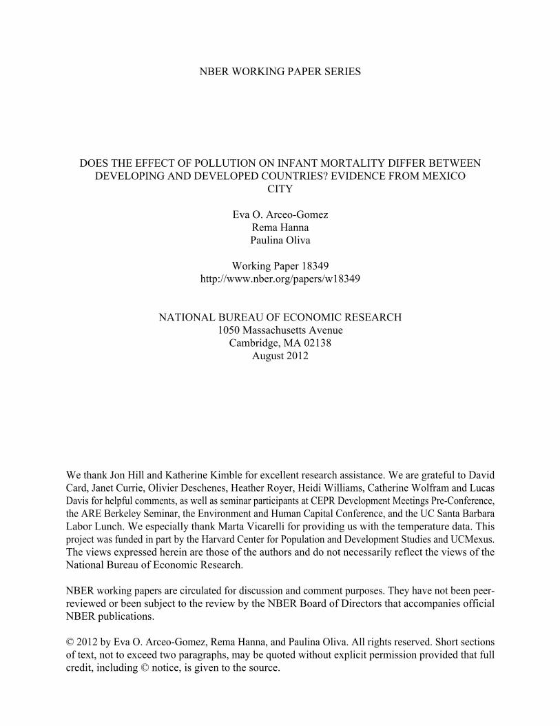
rise and can get trapped in the inversion (see Figure 1). As the sun energy equates the

temperatures of the cold and hot air masses, the "lid" effect disappears (the inversion “pops”),

and the pollutants rise again. Inversions may have substantial effects on the concentration levels

of certain types of pollutants, particularly primary pollutants (CO, particulate matter, NO, NOx,

and SOx, VOC) that may be released in the morning rush hours when the inversions typically

occur (Jacobson, 2002). Out of the primary pollutants, we would, therefore, expect the largest

effects for pollutants in which vehicles comprise a large share of their emissions. For example,

in Mexico City, 98 percent of CO emissions came from vehicles in 1998, and therefore, we

expect that a large share is released in the morning commute hours. In contrast, we may expect

weaker effects for pollutants like particulate matter, in which 36 percent is released by vehicles,

or SO2, in which only 21 percent is.

Inversions may have muted effects on secondary pollutants (O3, NO2, sulfuric acid),

which require time to mix from the primary pollutants, and therefore, may only appear later in

the day when it is likely that the inversions have already “popped” (Jacobson, 2002). Moreover,

inversions may inhibit the formation of these pollutants in other ways. For example, in the

particular case of O3, given that the chemical reactions that result in O3 require warmth and

                                                            9 See for example, Secretaría del Medio Ambiente del Distrito Federal, "Informe Climatológico Ambiental del Valle de México," 2005. 

7  

sunlight, the thick layers of pollution associated with thermal inversions may interfere with O3

formation.10

We can, therefore, formally test whether inversions increase the concentrations of

different types of pollutants (Equation 3) and, if so, we can use the number of thermal inversions

in a given week ( to instrument for pollution in Equation 4:

Equation 3: ∑ ℎ

Equation 4: ∑ ℎ

Note that varies at the week level, and therefore, week fixed effects are no longer identified

and errors may also be correlated within weeks.11 We therefore control for municipality-specific

week trends (w) and allow for errors to be clustered at the week level. We also include for

municipality fixed effects ( to control for time-invariant characteristics across municipalities,

and year fixed effects ( to account for city-wide year trends, such as recessions.12

Importantly, we include a flexible set of controls for temperature and weather conditions

(ℎ ) that includes a fourth polynomial in mean temperature, a third degree polynomial in

minimum and maximum temperatures during the week, a second degree polynomial in

precipitation, cloud cover and humidity measures. Controlling for temperature is important for

the exclusion restriction to hold, since inversions have a clear seasonal pattern and temperature

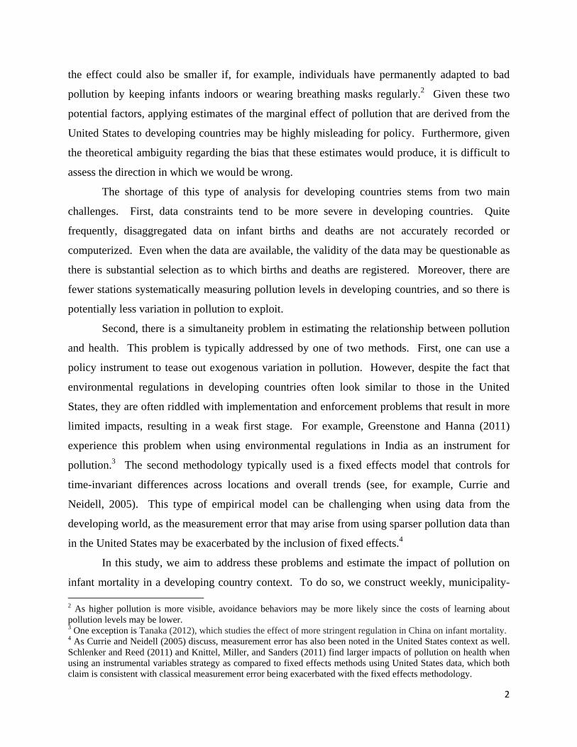
may independently affect infant mortality (Deschenes and Greenstone, 2011).13 Figure 2, Panel

A shows the average number of thermal inversions per week for each month of the year (bars), as

well as the average temperatures for each month of the year (spikes) measured by the right axis.

As expected, given the conditions necessary for a radiation inversion, a large share of the

inversions occurs in the winter (November-March). However, inversions also occur in months

with relatively high temperatures (April, May and October), which will allows us to disentangle

the effects of temperature on infant mortality from that of air pollution.

                                                            10 Ozone Formation, EPA, http://www.epa.gov/oar/oaqps/gooduphigh/bad.html#6 11 Note that as we exploit week-to-week variation within municipalities in this setting, sorting across different municipalities due to differential pollution should not be a large concern. Moreover, Hanna and Oliva (2011) show that sorting is nonetheless not a large concern within Mexico City as very few households move across census blocks, which are an even smaller geographic unit than municipalities. 12 As we illustrate below, our results are robust to different configurations of the control variables, such as omitting controls for minimum and maximum temperatures during the week, omitting municipality-specific time trends and including seasonal effects. 13 In addition, including precipitation, cloud cover and humidity is also essential as it is possible that an inversion can lead to a thunderstorm if moisture is trapped in the inversion.

8  

Note three additional specification details. First, all regressions are clustered at the week

level, which is the level of variation of our instrument. However, our estimates are robust to

alternative modeling assumptions for the error term; for example, our reduced form results

remain unchanged if we employ Conley standard errors to adjust for geospatial correlations (see

Appendix Table 1). Second, all regressions are weighed by the number of births in the

respective cohort (Appendix 1 also shows that the results are not sensitive to the weights). Third,

we can also try to disentangle the effects of different pollutants on infant health by taking

advantage of the fact that the inversion effect may vary based on the geographical features of a

location, such as its altitude. Specifically, this will allow us to create multiple instruments for

the pollution variables.

Finally, in addition to estimating the marginal effect of a change in average pollution, we

explore whether there is a non-linear dose-response relationship between pollution and infant

mortality. We estimate our IV model using a linear spline in pollution with a single node that

roughly corresponds to the range in each pollutant in Currie and Neidell (2005). In particular,

we use a cutoff of one standard deviation above the mean pollutant value in Currie and Neidell

(2005) to generate the splines.14 This allows us to assess whether our results differ from

previous studies in the United States due to non-linearities in the health-mortality relationship.

II.C. Data

We compiled a comprehensive dataset on pollution measures, weather conditions, and mortality

for Mexico City for the years 1997-2006. Each data source is described in detail below.

Neonatal and Infant Mortality

We constructed the mortality measures from data that we obtained for the Mexico City

Metropolitan Area (MCMA) from the Ministry of Health (Secretaría de Salud Pública). We

utilize two sources. First, we compiled data from death certificates, including information on

day of death, gender of the child, municipality of residence, age of the child at death, and cause

of death. Second, to compute mortality rates, we additionally gained access to the birth

certificate registry, which contains information on date of birth and municipality of residence.

                                                            14 We additionally test the robustness of the results to different definitions of the splines.

9  

We then computed weekly, municipality-level neonatal mortality rates (those that are 28

days of age and younger) and infant mortality rates (those that are one year old and younger).

To do so, for each week-municipality observation, we calculate the number of births in the last

28 days and in the last year.15 Mortality rates are then calculated by dividing the total number of

deaths in each week-municipality by the total number of live births in the corresponding age

group and then multiplying by 100,000. Thus, our coefficients can be interpreted as the number

of deaths in a week per 100,000 children born alive in the respective age cohort.

Pollution

Pollution data are notoriously absent in many developing countries. When available, they are

often only cross-sectional, or of mixed quality. In this paper, we are able to take advantage of a

relatively rich, panel dataset that is available for Mexico City, namely the Automatic Network of

Atmospheric Monitoring (RAMA). Measures are available for particulate matter under 10

micrometers (PM10), sulfur dioxide (SO2), carbon monoxide (CO) and ozone (O3). These data

are considered to be of high quality, and, as Davis (2008) points out, “[t]hese measures are

widely used in scientific publications...” However, it is important to note that they are drawn

from relatively few stations: PM10 is available for 10 stations from 1997 to 1999, and from 16

stations starting in 2000, SO2 is drawn from 26 stations, CO is drawn from 24 stations and O3 is

drawn from 21 stations.

From these data, we construct weekly measures of pollution for each of the 56

municipalities in Mexico City using the inverse of the distance to nearby stations as weights (see

Currie and Neidell (2005) for description of the methodology). Out of the 56 municipalities in

Mexico City for which we have infant mortality data, we include the 48 that are within 15

kilometers of a station. There is a tradeoff between constraining the sample to municipalities

that are even closer to at least one station for greater precision of the pollution measure and

increasing the distance cutoff to include more municipalities. As shown in Appendix Table 2,

our results are robust to different definitions of this cutoff.

We use the hourly measures of pollution to calculate the maximum daily 8-hour average

for CO and average this over the week, the maximum daily 24-hour average for PM10 and

                                                            15 Since 0.03 percent of the births certificates have missing month and day of birth, we adjust weekly estimates of births by dividing un-dated births equally among all weeks of the year.

10  

average this over the week, and then weekly averages for SO2 and for O3.16 All of these daily

measures are then averaged over the week.

Thermal Inversions

Thermal inversions are recorded by the Meteorological Unit of the local Ministry of

Environment. They conduct screenings almost every day, which consist of measuring hourly

temperatures at different altitudes using an aerostatic balloon.17 The existence of an inversion is

determined upon finding non-monotonic temperature gradients. Records are kept on the time

and temperature of the inversion rupture, so that one can also compute the number of hours an

inversion lasted, as well as the thickness of its layer. We aggregate the data to the weekly level

by computing the number of thermal inversions in a given week. To test non-linear effects of

pollution on infant mortality, we can also create indicator variables for 1, 2-3 and 4-7 thermal

inversions per week.

Temperature and Weather

We obtained temperature and weather variables as additional controls in our specification.

Hourly temperature measures are available from 24 stations in the RAMA network, and daily

level measures of humidity, precipitation and cloud measures are available daily from 219 local

weather stations. Using the same methodology to compute weekly, municipality-level measures

of pollution, we use this information to compute the temperature and weather controls.

II.D. Data Description

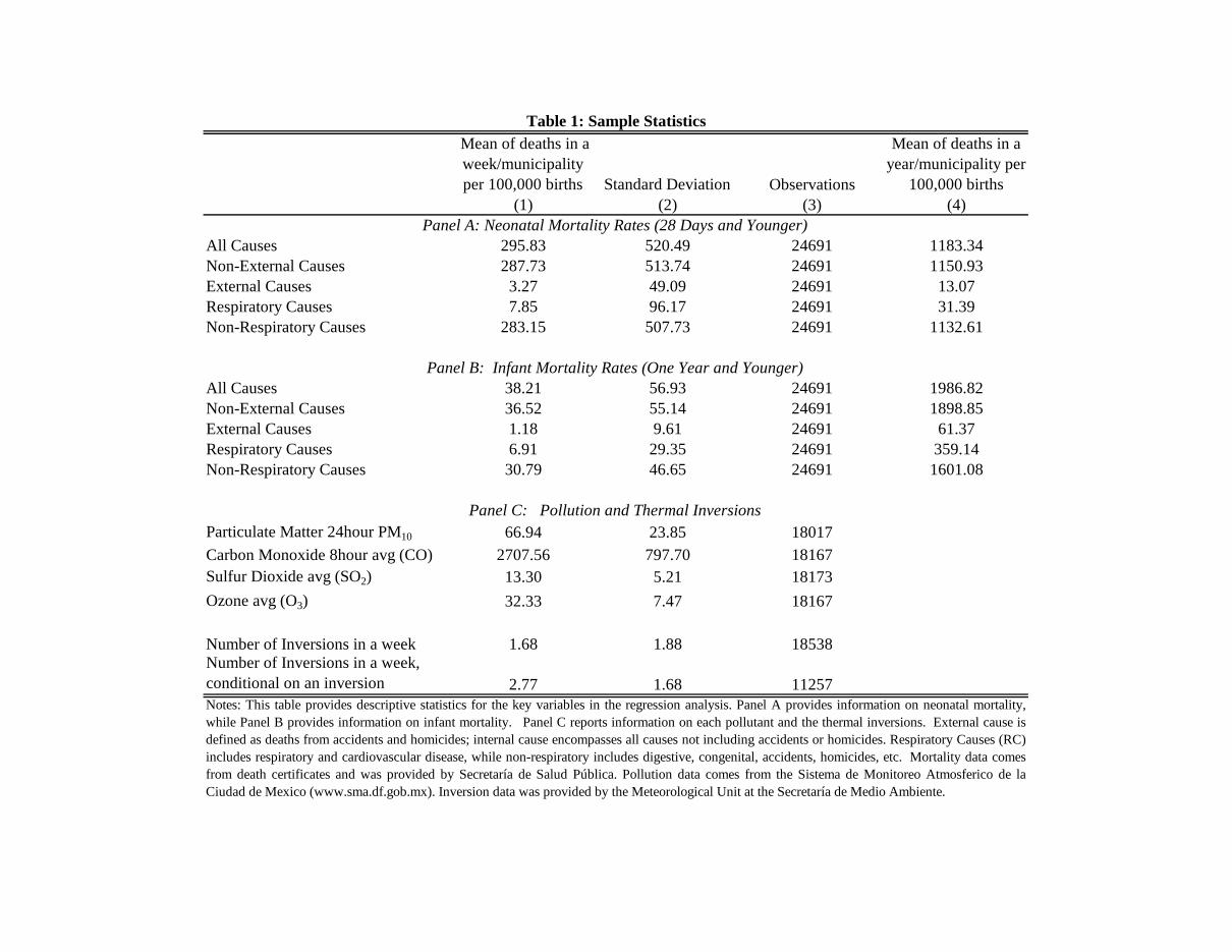
We describe the data in Table 1. In Panel A and B, we provide information on neonatal

mortality rates (for children that are 28 days and younger) and infant mortality rates (those that

are one year and younger) respectively. In addition to the means for the weekly measures used

in the regression analysis (Column (1)), we additionally include the mean across municipalities

in a given year per 100,000 births for ease of comparison with the U.S. figures (Column (4)).18

                                                            16 We use these measures for ease of comparison with Currie and Neidell (2005) and Knittel et al. (2011). However, our results are robust to alternative measures of pollution. 17 Of the 3,652 days within our sample period, we have data on whether an inversion occurred for 95 percent of these days. We drop the weeks in which we are missing inversion data. 18 Note that the weekly measure for infant deaths in Column 1 appears smaller than that of neonatal mortality, despite the fact that the later also includes neonatal deaths. The difference in magnitudes is mainly due to scaling:

11  

Over the period of study, yearly mortality rates are more than double in Mexico City than in the

United States: The neonatal mortality rate is 1183, while the U.S. rate is 460. Similarly, the

infant mortality rate in Mexico City was 1986, while the comparable US figures was 698.

Note that, we also provide mortality estimates, by cause of death. We can test whether

the effect of pollution on mortality is driven by deaths that we expect to be related to pollution.

We define this comparison in two ways. First, we can compare all internal deaths with all

external deaths (i.e., accident, homicides). This is a very strict definition, in that it assumes that

pollution affects all internal deaths, including for example those from digestive diseases, which

may or may not be affected by pollution. Moreover, there are relatively fewer deaths from

external sources (61.37 per 100,000), with relatively less variation, and so we may not capture an

effect with the same sample size due to power concerns. Therefore, we also compare diseases

that are more likely to be directly attributed to pollution (i.e., respiratory and cardiovascular

disease) versus those that are less likely to be directly attributed to pollution (digestive,

congenital, accidents, homicides, etc.).

In Panel C, we provide means for particulate matter of 10µm or less (PM10), carbon

monoxide (CO), ozone (O3), and sulfur dioxide (SO2), as well as summary information on

inversions.19 Despite falling pollution levels in Mexico City, the average is still quite high. For

example, the mean level of PM10 is about 67µm as compared to 39.45µm observed in California,

as documented by Currie and Neidell (2005). Inversions are fairly frequent: on average, there

are 1.7 inversions in a municipality-week. Conditional on an inversion occurring that week,

there is an average of 2.77 inversions in a municipality-week.

III. RESULTS

III.A. Correlations in Pollution and Health

Before we turn to the quasi-experimental approaches, we first describe the evolution of pollution

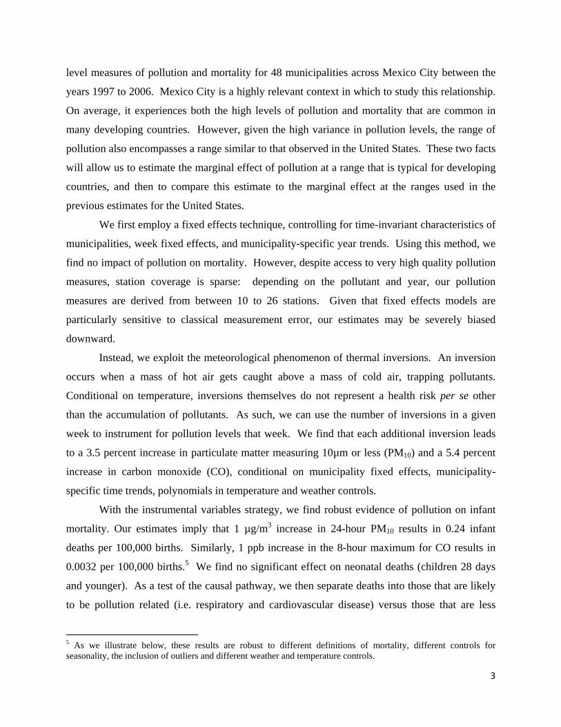
and infant mortality over time. In Figure 3, we graph average weekly neonatal (Panel A) and

infant mortality rates (Panel B) against each of the four air pollutants over time. Mexico City has                                                                                                                                                                                                 neonatal mortality rates are computed by dividing the number of deaths occurred in a single week within the 28 day cohort by the number of live births corresponding to that cohort. Hence, the denominator for the neonatal mortality figure is necessarily smaller than the denominator for the infant mortality figure. Column 4 shows mortality rates on a yearly basis. This column is computed by multiplying Column 1 by 4 (or 52/13) in the case of neonatal mortality and by 12 in the case of infant mortality. 19 Given the presence of outliers in the data, we trim the top and bottom 1 percent of values. The primary results remain largely unchanged if we do not trim the outliers as shown in Columns 5 and 6 of Appendix Table 4.

12  

been successful in reducing pollution city-wide over the 1997 to 2006 time period, with all four

air pollutants falling sharply over this period (Molina and Molina, 2002). As the figures

illustrate, mortality rates are also falling and, in some cases, the rates closely track pollution

changes.

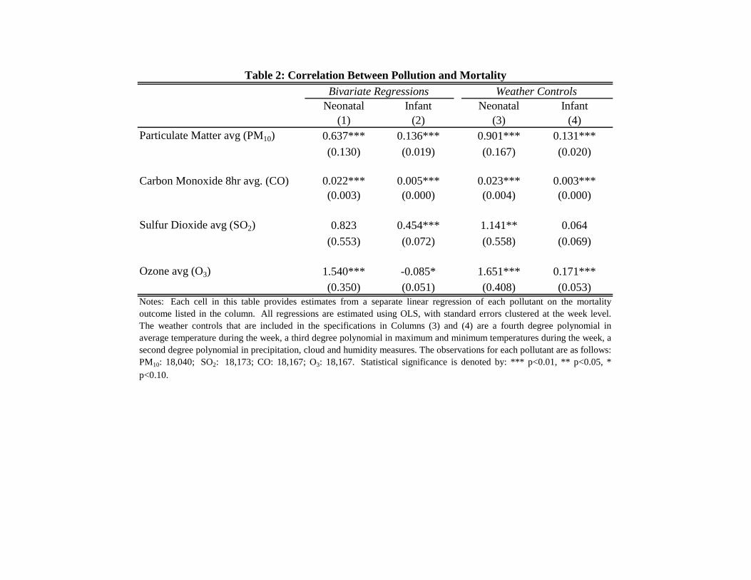
Table 2 quantifies these patterns. Specifically, we estimate Equation 1 for neonatal

mortality (Column (1)) and infant mortality (Column (2)). As the figure illustrates, we find a

large, significant, positive correlation, which is robust to the inclusion of flexible controls for

temperature and weather variables (Columns (3) and (4)). The magnitudes are fairly large: for

example, as shown in Column 4, a one µg/m3 increase in PM10 (1.5 percent increase) is

associated with 0.131 more infant deaths per 100,000 births per week, a one ppb (about 0.037

percent increase) in CO is linked to 0.003 more deaths, and a one ppb increase in O3 (a 3 percent

increase) is associated with 0.171 more deaths.

III.B. First Stage Estimates

We begin by examining the relationship between the occurrence of an inversion and each of the

four pollutants (PM10, CO, O3, and SO2), which comprises the first stage of our instrumental

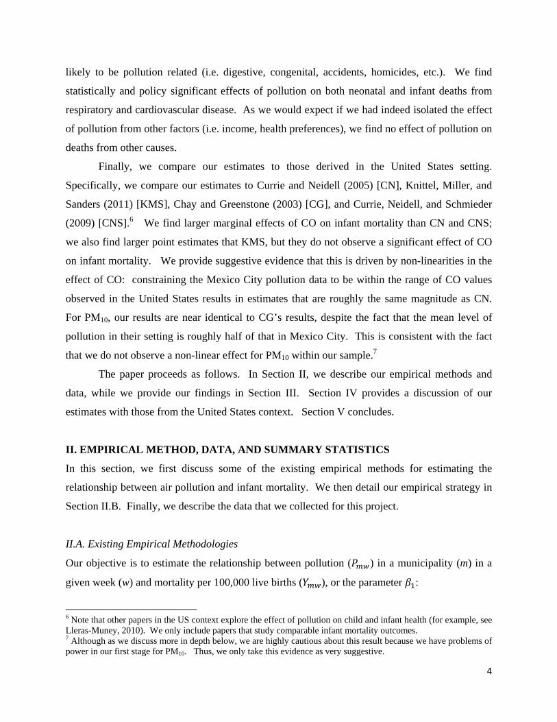
variables strategy. In Figure 4, we graph the average pollutant level by number of inversions.

As the figure illustrates, we observe a strong, and fairly linear, relationship between the number

of inversions the last week and PM10 and CO levels. In contrast, there does not appear to be an

obvious relationship between the number of inversions and either O3 or SO2.

We provide the corresponding regression analysis in Table 3. Specifically, we present

coefficient estimates from Equation 3. As suggested by the figure, inversions have a large and

significant effect on PM10 and CO. One additional inversion in the last week results in a 2

µg/m3, or 3.4 percent, increase in PM10 (Column 1). Similarly, one additional inversion results

in a 153 ppb, or 5.6 percent, increase in CO (Column 2). The effects on PM10 and CO are both

significant at the 1 percent level. There are no significant effects of thermal inversions on SO2

and O3 (Columns 3 and 4). These overall findings are consistent with the theoretical predictions

discussed in Section II.

III.C. Causal Estimates of Pollution on Infant Mortality and Health

13  

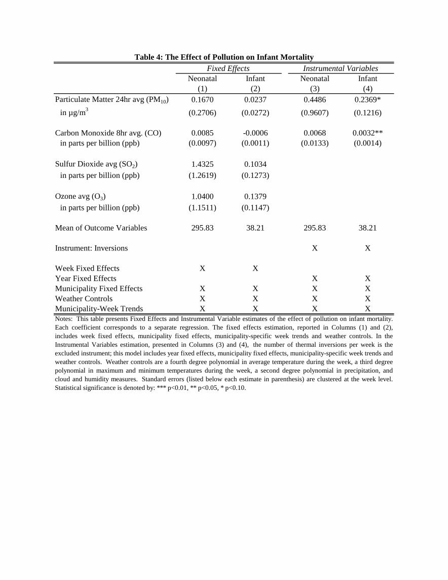
In Columns (1) and (2) of Table 4, we provide the coefficient estimates of the effect of each

pollutant on neonatal and infant mortality, respectively, from estimating Equation 2 (the fixed

effects model). Note that we additionally include municipality-specific week trends in this

model.20 In Columns (3) and (4), we provide our IV estimates for the individual effects of PM10

and CO on mortality; here, we report the coefficient estimates from Equation 4.21 As there is no

first stage result for SO2 or O3, we do not estimate an IV estimate for these pollutants.

Using a fixed effects strategy, we find no observable effects of pollution on mortality

(Columns (1) and (2)). As compared to the cross-sectional analysis with controls that is shown

in Columns (3) and (4) in Table 2, the fixed effects estimates, for the most part, tend to be small

in magnitude and much less precisely estimated. This is consistent with classical measurement

error.

Instead, we turn to our instrumental variables strategy. Here, we find large effects of

pollution on infant mortality, but smaller and non-significant effects on neonatal mortality. In

the case of infant mortality, a one µg/m3 increase in PM10 over the week leads to 0.23 deaths per

100,000 births, while a one ppb increase in CO leads to 0.032 deaths.22 This implies that a 1

percent increase in PM10 over a year leads to a 0.42 percent increase in infant mortality, while a 1

percent increase in CO results in a 0.23 percent increase. These findings are consistent with the

fact that death by respiratory diseases, which are likely affected by pollution exposure, are higher

share of total deaths for infants than for those under 28 days, and may reflect underlying

differences in ambient air exposure (i.e. infants may be more likely to be taken outside during the

day than newborns).

One concern is that models that estimate the effect of pollution on infant death within a

short timeframe, such a week, overstate the effect. This bias would occur if pollution simply

accelerates infant deaths by a short time period rather than causing additional deaths

                                                            20 As Appendix Table 3A shows, the results do not qualitatively change if we drop the municipality week trends (Columns (1) and (2)), include fewer temperature controls (Columns (3) and (4)), or drop the week fixed effects so that the estimate is more comparable to Currie and Neidell (2005) (Columns (5) and (6)). 21 Appendix Table 3B explores the robustness of the IV estimates to different control variables. As shown in Columns (1) and (2), the effects on neonatal and infant mortality are qualitatively similarly if we do not include the municipality-week trends, which suggest the inversions are for the most part uncorrelated with the trends in mortality that are unrelated to pollution. Relaxing the temperature controls (Columns (3) and (4)) leads to larger estimates for infant mortality, but the effects are still not significant for neonatal mortality. Including a more flexible time trend (Columns (5) and (6)) also results in qualitatively similar results. 22 Note that Table 4 reports effects of CO in terms of neonatal/infant deaths associated with one part per billion, which corresponds to an increase in CO concentration of 0.037 percent.

14  

(“harvesting”). We do not find evidence of this. We can see this in two ways. First, the effect

on neonatal deaths is much smaller in magnitude than infant deaths. Due to the scaling, we need

to multiply the infant mortality estimates to compare the neonatal and infant mortality estimates.

When doing this, it becomes apparent that the effects on neonatal mortality are not only

insignificant, but also 50 percent smaller in magnitude. The fact that we find smaller effects of

air pollution on children below the age of 28 days suggests that air pollution is not accelerating

death of already vulnerable children, but is causing death of children with otherwise long life

expectancies. Second, in Appendix Table 4A and 4B, we present the results of our analysis

when we aggregate the data to the month level rather than at the week level. If harvesting is an

issue of concern with our estimates, we would expect smaller effects when using data aggregated

at the month level. However, this is not the case.23

It is important to note that our IV results are very robust to changes in the model

specification, providing a high level of confidence in this strategy. In Appendix Table 5, we first

test whether our results are driven by changes in the denominator of the left hand side variable,

i.e., the number of births. This would be the case if pollution shocks have an impact in the

number of live births in the current week, which are included in the denominator. We perform

this check by estimating our IV model with the log of deaths as a dependent variable and the log

of births as an additional control variable. The results of this specification, reported in Columns

(1) and (2), can be compared with our main results divided by the average mortality rate. We

find that the results of the log specification for infant mortality are slightly smaller, but not

significantly different than our main estimates, and they are still significant at the 10 percent

level (the effects on neonatal remains insignificant across both models). Thus, it is unlikely that

the results are driven by changes in births.24

Second, we explore whether the seasonality in thermal inversions is driving our results.

This could be the case if our temperature and weather variables are not fully controlling for

climatic differences across seasons, or if the flu or other epidemics have similar timing with

                                                            23 To make the magnitudes of infant mortality coefficients comparable across Appendix Table 4B and our main results (Table 4), it is useful to compute the yearly mortality effects associated with both (i.e., multiplying coefficients in Table 4 (Column 2) by 52 and the coefficients in Appendix Table 4B (Column 2) by 12). The coefficients from monthly aggregated data appear about three times as large as the coefficients from weekly aggregated data. Note, however, that only the coefficients from the CO IV regression are reliable since the first stage for PM10 is lost when aggregating data at such a coarse level (See Appendix Table 4A). 24 Note that in Columns (3) and (4) of Appendix Table 5, we also show the estimates had we not dropped the top and bottom 1 percent of values in pollution and show that the results are not sensitive to their inclusion.

15  

thermal inversions, but are not fully controlled for by our temperature and weather variables.

We do this in several ways. First, we can control for mortality in the second largest city of

Mexico, Guadalajara, which shares similar weather patterns as Mexico City, but does not

experience inversions. As Appendix Figure 1 illustrates, Guadalajara also experience seasonal

patterns in mortality, albeit not as pronounced as in Mexico City. Including the mortality rate in

Guadalajara as a control (Columns (1) and (2) of Appendix Table 6A) does not qualitatively

affect the results; the effect of CO, if anything, actually increases when we control for the

mortality rate in Guadalajara. Second, we can directly include season fixed effects (Columns (3)

and (4) of Appendix Table 6A). The magnitude of the results remains qualitatively unchanged.

However, note that if we include both season and year fixed effects, the standard errors increase

substantially even though the magnitude of the estimates remains unchanged (Columns (4) and

(5)). Third, we can confirm whether the effect of pollution is similar across seasons, particularly

whether it differs across the winter and summer months. Appendix Table 6B shows these

results.25 Note that we observe a significant first stage for both the summer and winter months.26

On net, the effects on infant mortality do not appear to be significantly different across the winter

and summer months.

Next, in Table 5, we replicate the IV analysis for mortality that results from different

causes. This can be viewed as a placebo test: If we find that our pollution measure is resulting

in deaths that are unlikely to be related to pollution, we would conclude that our instrument

might be directly linked to unobserved socio-demographic determinants of mortality. We can

define pollutant-related deaths in two ways. First, we compare deaths from all types of internal

sources and those from purely external sources. We find no observable effect on either internal

or external effects for neonatal (Columns 1 and 2). The effect of pollution on infant mortality

appears to be driven by internal deaths (Column 6); there is no observable effect on external

deaths for infants. However, mortality from external sources is rare compared to that from

internal sources, meaning it would be more difficult to detect an effect on external deaths if there

indeed is one. Moreover, it is possible that external deaths are simply accidental and/or

immediate, and thus are altogether uncorrelated with income or health care quality.

                                                            25 For completeness, we show two possible definitions of seasons. Specifically, we can define summer from week 13 to week 42 (Columns 1 and 2) or from week 14 to 43 (Columns 3 and 4). The results are qualitatively similar across the two definitions. 26 The Angrist-Pischke F-statistics are above the Stock-Yogo 10 percent threshold for weak instruments.

16  

Therefore, we can also classify deaths by those that are more likely to be attributed to

pollution (i.e., respiratory and cardiovascular disease) versus those from sources that are less

likely (digestive, congenital, accidents, homicides, etc.). This is not a perfect separation, as

children who are weakened by high pollution may be more likely to pass away from other

sources (such as digestive disorders) and causes of death may be imperfectly diagnosed.

However, we should still expect the effect on respiratory diseases to be relatively large if

pollution is driving much of the effect, and not other socio-demographic characteristics. Our

results suggest that most of the deaths related to pollution are linked to respiratory and

cardiovascular causes: We find no effect on non-respiratory deaths for either neonatal (Column

3) or infant (Column 7) deaths. Importantly, if we focus on deaths from respiratory and

cardiovascular disease, we find large effects of pollution on both infant (Column 8) and neonatal

(Column 4) deaths. The fact that we find that the effect of pollution on mortality is driven

mainly by respiratory causes implies that our instrument is capturing exogenous variation in

pollution, and not just trends in socioeconomic characteristics.

Finally, in all the regressions above, the effect for any individual pollutant may be

capturing its own effect, as well as the effect of other pollutants. This is particularly problematic

given that we have used one main instrument to identify the effect of each pollutant.

Alternatively, we can include all pollutants in the same specification, so that the estimated effect

of each pollutant is purged of potential bias from the others. This results in multiple endogenous

variables, and therefore, we need to identify multiple instruments in order to estimate the causal

effect of each pollutant, conditional on one another.

We exploit the fact that the effect of the inversions on pollution may differ based on the

altitude of the municipality and the thickness of the inversion, and create three instruments: the

number of inversions, the number of inversions interacted with altitude, and the thickness of

inversion interacted with altitude. As Appendix Table 7 illustrates, PM10 concentrations are

lower at higher altitudes, presumably because higher areas are likely to be above the thermal

inversion layer. However, altitude does not seem to matter as much for CO concentrations,

unless the thermal inversion layer is thick. Thickness of the thermal inversion induces higher

concentrations of CO at higher altitudes. The Angrist-Pischke F-statistic for both estimated

equations is above the Stock-Yogo 10 percent critical value for single endogenous regressors,

17  

which suggests that our instrument combination induces at least some independent variation in

both pollutants.

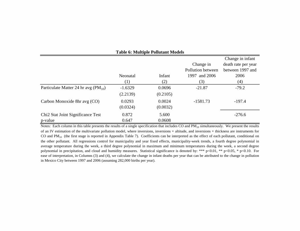
The IV estimates are presented in Table 6. We do not observe a significant effect of

either pollutant on neonatal mortality, and the two pollutant variables are jointly insignificant

Column (1)). While each pollutant is not an individually significant predictor for infant

mortality, the two pollutants are jointly significant in predicting infant mortality at the 10 percent

level (Column (2)).27 In terms of magnitude, we find that given the overall decline in pollution

in Mexico City from 1997 to 2006 (weighted by births), our estimates would predict a change in

the infant mortality rate that is due to pollution of 277 births per 100,000 (Columns (3) and (4)).

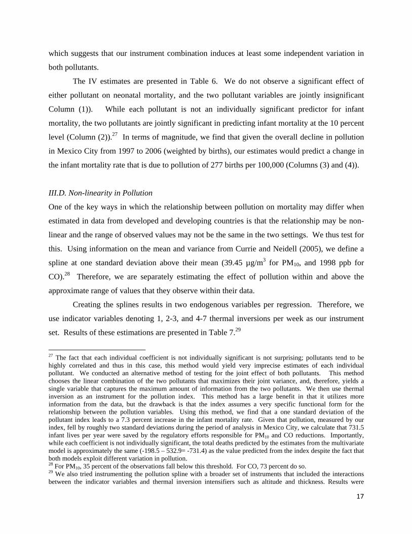
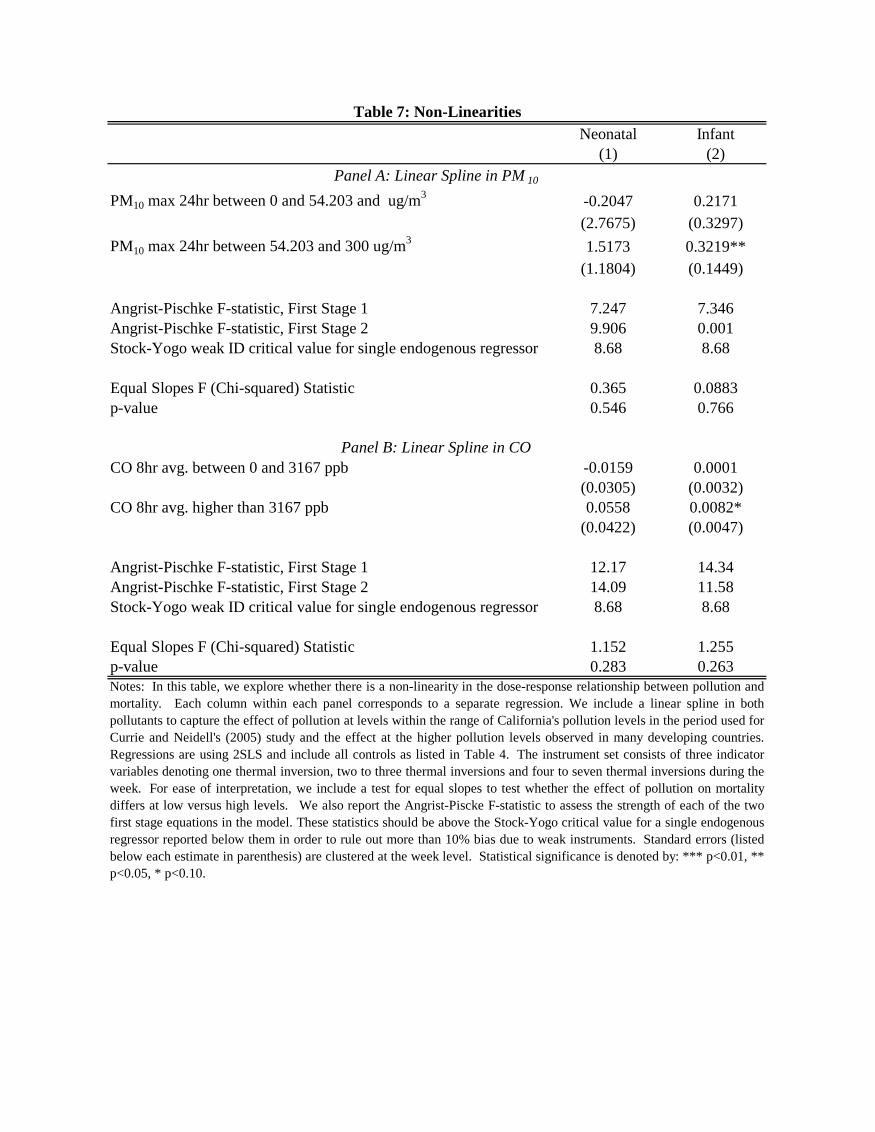
III.D. Non-linearity in Pollution

One of the key ways in which the relationship between pollution on mortality may differ when

estimated in data from developed and developing countries is that the relationship may be non-

linear and the range of observed values may not be the same in the two settings. We thus test for

this. Using information on the mean and variance from Currie and Neidell (2005), we define a

spline at one standard deviation above their mean (39.45 µg/m3 for PM10, and 1998 ppb for

CO).28 Therefore, we are separately estimating the effect of pollution within and above the

approximate range of values that they observe within their data.

Creating the splines results in two endogenous variables per regression. Therefore, we

use indicator variables denoting 1, 2-3, and 4-7 thermal inversions per week as our instrument

set. Results of these estimations are presented in Table 7.29

                                                            27 The fact that each individual coefficient is not individually significant is not surprising; pollutants tend to be highly correlated and thus in this case, this method would yield very imprecise estimates of each individual pollutant. We conducted an alternative method of testing for the joint effect of both pollutants. This method chooses the linear combination of the two pollutants that maximizes their joint variance, and, therefore, yields a single variable that captures the maximum amount of information from the two pollutants. We then use thermal inversion as an instrument for the pollution index. This method has a large benefit in that it utilizes more information from the data, but the drawback is that the index assumes a very specific functional form for the relationship between the pollution variables. Using this method, we find that a one standard deviation of the pollutant index leads to a 7.3 percent increase in the infant mortality rate. Given that pollution, measured by our index, fell by roughly two standard deviations during the period of analysis in Mexico City, we calculate that 731.5 infant lives per year were saved by the regulatory efforts responsible for PM10 and CO reductions. Importantly, while each coefficient is not individually significant, the total deaths predicted by the estimates from the multivariate model is approximately the same (-198.5 – 532.9= -731.4) as the value predicted from the index despite the fact that both models exploit different variation in pollution. 28 For PM10, 35 percent of the observations fall below this threshold. For CO, 73 percent do so. 29 We also tried instrumenting the pollution spline with a broader set of instruments that included the interactions between the indicator variables and thermal inversion intensifiers such as altitude and thickness. Results were

18  

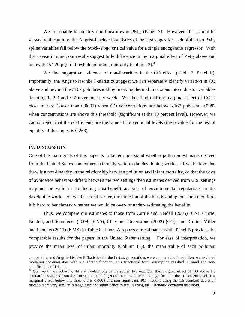
We are unable to identify non-linearities in PM10 (Panel A). However, this should be

viewed with caution: the Angrist-Pischke F-statistics of the first stages for each of the two PM10

spline variables fall below the Stock-Yogo critical value for a single endogenous regressor. With

that caveat in mind, our results suggest little difference in the marginal effect of PM10 above and

below the 54.20 µg/m3 threshold on infant mortality (Column 2).30

We find suggestive evidence of non-linearities in the CO effect (Table 7, Panel B).

Importantly, the Angrist-Pischke F-statistics suggest we can separately identify variation in CO

above and beyond the 3167 ppb threshold by breaking thermal inversions into indicator variables

denoting 1, 2-3 and 4-7 inversions per week. We then find that the marginal effect of CO is

close to zero (lower than 0.0001) when CO concentrations are below 3,167 ppb, and 0.0082

when concentrations are above this threshold (significant at the 10 percent level). However, we

cannot reject that the coefficients are the same at conventional levels (the p-value for the test of

equality of the slopes is 0.263).

IV. DISCUSSION

One of the main goals of this paper is to better understand whether pollution estimates derived

from the United States context are externally valid to the developing world. If we believe that

there is a non-linearity in the relationship between pollution and infant mortality, or that the costs

of avoidance behaviors differs between the two settings then estimates derived from U.S. settings

may not be valid in conducting cost-benefit analysis of environmental regulations in the

developing world. As we discussed earlier, the direction of the bias is ambiguous, and therefore,

it is hard to benchmark whether we would be over- or under- estimating the benefits.

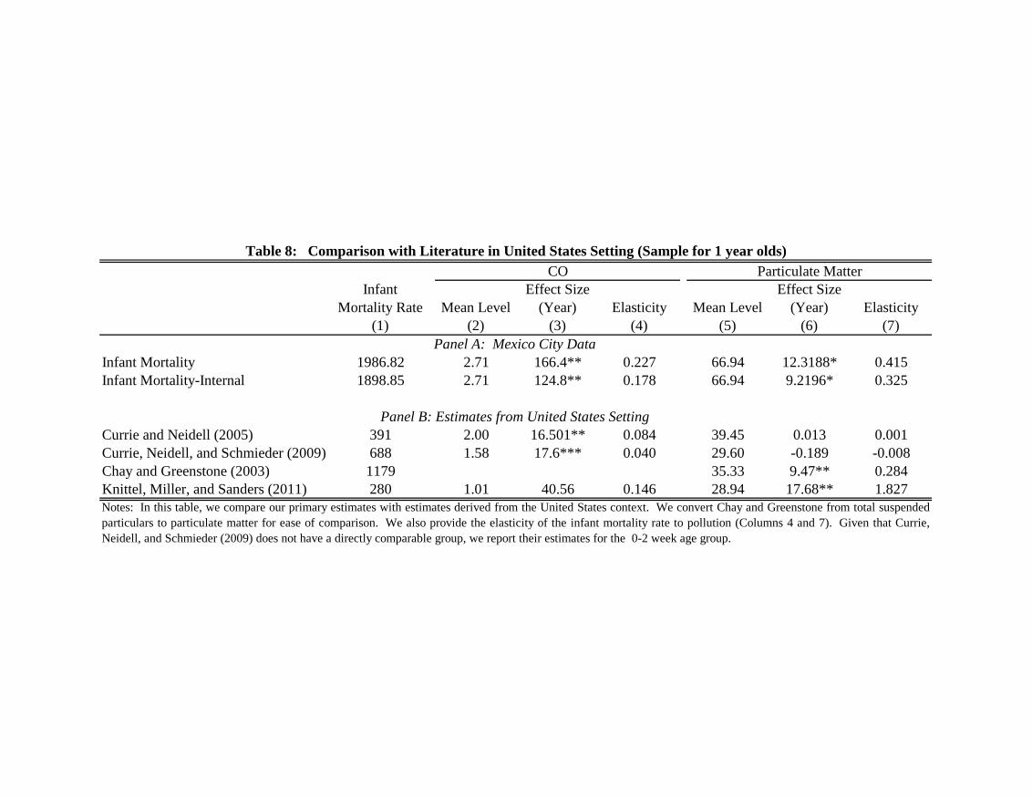
Thus, we compare our estimates to those from Currie and Neidell (2005) (CN), Currie,

Neidell, and Schmieder (2009) (CNS), Chay and Greenstone (2003) (CG), and Knittel, Miller

and Sanders (2011) (KMS) in Table 8. Panel A reports our estimates, while Panel B provides the

comparable results for the papers in the United States setting. For ease of interpretation, we

provide the mean level of infant mortality (Column (1)), the mean value of each pollutant                                                                                                                                                                                                 comparable, and Angrist-Pischke F-Statistics for the first stage equations were comparable. In addition, we explored modeling non-linearities with a quadratic function. This functional form assumption resulted in small and non-significant coefficients. 30 Our results are robust to different definitions of the spline. For example, the marginal effect of CO above 1.5 standard deviations from the Currie and Neidell (2005) mean is 0.0105 and significant at the 10 percent level. The marginal effect below this threshold is 0.0008 and non-significant. PM10 results using the 1.5 standard deviation threshold are very similar in magnitude and significance to results using the 1 standard deviation threshold.

19  

(Columns (2) and (5)), the point estimates (Columns (3) and (6)), and the elasticity (Columns (4)

and (7)). Note several features regarding the table. First, we use the estimates from the single

pollutant models because our subset of pollutants differs from these papers. Even though the

models are not fully comparable, we replicate this table using the multiple pollutant models in

Appendix Table 8 for completeness. Second, note that CG study total suspended particulates

(TSP) and not PM10. For comparability to our estimates, we follow KMS and convert the TSP

estimates using the following formula: PM10 = 0.55 TSP. Third, CG and KMS study internal

deaths rather than all deaths, so we additionally report the estimates for internal deaths for our

sample. Finally, we put all estimates at the year level for ease of comparison.

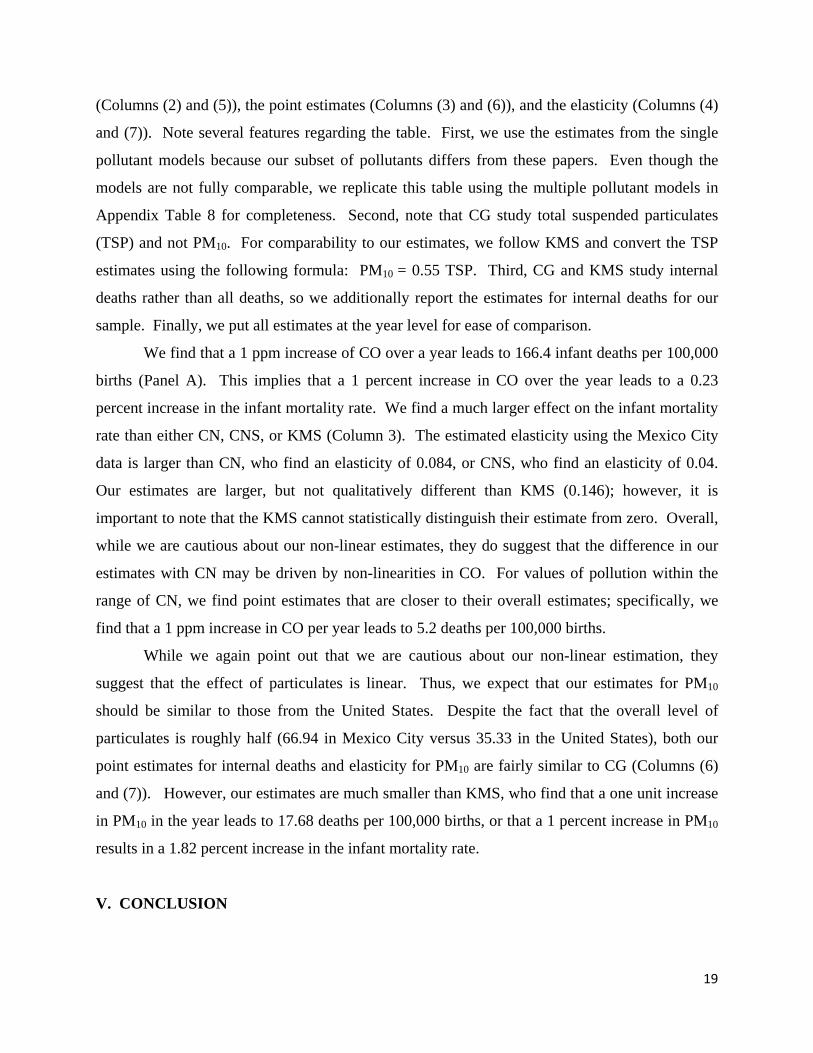
We find that a 1 ppm increase of CO over a year leads to 166.4 infant deaths per 100,000

births (Panel A). This implies that a 1 percent increase in CO over the year leads to a 0.23

percent increase in the infant mortality rate. We find a much larger effect on the infant mortality

rate than either CN, CNS, or KMS (Column 3). The estimated elasticity using the Mexico City

data is larger than CN, who find an elasticity of 0.084, or CNS, who find an elasticity of 0.04.

Our estimates are larger, but not qualitatively different than KMS (0.146); however, it is

important to note that the KMS cannot statistically distinguish their estimate from zero. Overall,

while we are cautious about our non-linear estimates, they do suggest that the difference in our

estimates with CN may be driven by non-linearities in CO. For values of pollution within the

range of CN, we find point estimates that are closer to their overall estimates; specifically, we

find that a 1 ppm increase in CO per year leads to 5.2 deaths per 100,000 births.

While we again point out that we are cautious about our non-linear estimation, they

suggest that the effect of particulates is linear. Thus, we expect that our estimates for PM10

should be similar to those from the United States. Despite the fact that the overall level of

particulates is roughly half (66.94 in Mexico City versus 35.33 in the United States), both our

point estimates for internal deaths and elasticity for PM10 are fairly similar to CG (Columns (6)

and (7)). However, our estimates are much smaller than KMS, who find that a one unit increase

in PM10 in the year leads to 17.68 deaths per 100,000 births, or that a 1 percent increase in PM10

results in a 1.82 percent increase in the infant mortality rate.

V. CONCLUSION

20  

There is a growing concern about the effects of pollution on health in the developing world.

Especially in their urban areas, high population densities and low quality health services are

colliding with high levels in harmful pollutant concentrations. This paper sheds light on the

importance of air quality improvements in the effort to curtail mortality rates.

Using a novel instrumental variables strategy, we find statistically significant effects of

pollution on infant mortality in Mexico City. Our estimates imply that a 1 ppb increase in CO

over a week leads to a 0.0032 per 100,000 births increase in the infant mortality rate, while a 1

µg/m3 increase in PM10 leads to a 0.24 per 100,000 births increase in their mortality rate. This

implies that a 1 percent increase in PM10 over a year leads to a 0.42 percent increase in infant

mortality, while a 1 percent increase in CO results in a 0.23 percent increase. Our results on CO

are generally larger than those estimated with data from the United States, while we find

comparable results for PM10 despite the fact that pollution levels are more than double in Mexico

City. This is consistent with our suggestive evidence of a non-linear relationship between CO

and infant mortality, and a linear relationship between PM10 and mortality. Thus, our findings

suggest that using U.S. data to estimate the benefits from cleaner air in the developing world may

be biased for pollutants that exhibit a non-linear relationship between pollution and mortality.

21  

WORKS CITED

Bell, M.L, and D.L. Davis, “Reassessment of the Lethal London Fog of 1952: Novel Indicators of Acute and Chronic Consequences of Acute Exposure to Air Pollution,” Environmental Health Perspectives, 109(2001), 389–394. Chay, Kenneth, and Michael Greenstone, “The Impact of Air Pollution on Infant Mortality: Evidence from Geographic Variation in Pollution Shocks Induced by a Recession,” Quarterly Journal of Economics, 118(2003), 1121-1167. Currie, Janet, and Matthew Neidell, “Air Pollution and Infant Health: What Can We Learn from California’s Recent Experience?” Quarterly Journal of Economics, 120(2005), 1003-1030. Currie, Janet, Matthew Neidell, and Johannes Schmieder, “Air Pollution and Infant Health: Lessons from New Jersey,” Journal of Health Economics, 28 (2009), 688 – 703. Davis, Lucas W., “The Effect of Driving Restrictions on Air Quality in Mexico City,” Journal of Political Economy, 116(2008), 38–81. Deschenes, Olivier, Michael Greenstone, and Joseph Shapiro, “Defending Against Environmental Insults: Drugs, Emergencies, Mortality and the NOx Budget Program Emissions Market,” Working Paper, 2012. González Calderón, Martha Hilda et al., “Informe Climatológico Ambiental del Valle de México,” Secretaría del Medio Ambiente, 2005. Greenstone, Michael, and Rema Hanna, “Environmental Regulations, Air and Water Pollution and Infant Mortality in India,” NBER Working Paper No. 17210, 2011. Hanna, Rema and Paulina Oliva, “The Effect of Pollution on Labor Supply: Evidence from a Natural Experiment in Mexico City,” NBER Working Paper No. 17302, 2012. Jacobson, M., Atmospheric Pollution. History, Science, and Regulation, 1st ed. (Cambridge, UK: Cambridge University Press, 2002). Jayachandran, Seema, “Air Quality and Early-Life Mortality during Indonesia’s Massive Wildfires in 1997,” Journal of Human Resources, 44(2009), 916–954. Knittel, Christopher, Douglas L. Miller, and Nicholas J. Sanders, “Caution, Drivers! Children Present: Traffic, Pollution, and Infant Health,” National Bureau of Economic Research Working Paper No. 17222, 2011. Lleras-Muney, Adriana, “The Needs of the Army: Using Compulsory Relocation in the Military to Estimate the Effect of Environmental Pollutants on Children's Health,” Journal of Human Resources, 35 (2010), 549-590.

22  

Molina, Luisa T., and Mario J. Molina. Air Quality in the Mexico Megacity: An Integrated Assessment. Dordrecht: Kluwer Academic Publishers, 2001. Moretti, Enrico, and Matthew Neidell, “Pollution, Health, and Avoidance Behavior: Evidence from the Ports of Los Angeles,” Journal of Human Resources, 46(2011), 154–75. OECD, “OECD Environmental Outlook to 2050: The Consequences of Inaction,” Publications de l'OCDE, 2012. Schlenker, Wolfram, and W. Reed Walker, “Airports, Air Pollution, and Contemporaneous Health,” National Bureau of Economic Research Working paper No. 17684, 2011.  

Tanaka, Shinsuke, “Environmental Regulations on Air Pollution in China and Their Impact on Infant Mortality,” Working Paper, 2012. Zivin, Joshua Graff and Matthew Neidell, “Days of haze: Environmental Information Disclosure and Intertemporal Avoidance Behavior,” Journal of Environmental Economics and Management, 58(2009), 119-128.

Mean of deaths in a week/municipality per 100,000 births Standard Deviation Observations

Mean of deaths in a year/municipality per

100,000 births(1) (2) (3) (4)

All Causes 295.83 520.49 24691 1183.34Non-External Causes 287.73 513.74 24691 1150.93External Causes 3.27 49.09 24691 13.07Respiratory Causes 7.85 96.17 24691 31.39Non-Respiratory Causes 283.15 507.73 24691 1132.61

All Causes 38.21 56.93 24691 1986.82Non-External Causes 36.52 55.14 24691 1898.85External Causes 1.18 9.61 24691 61.37Respiratory Causes 6.91 29.35 24691 359.14Non-Respiratory Causes 30.79 46.65 24691 1601.08

Particulate Matter 24hour PM10 66.94 23.85 18017

Carbon Monoxide 8hour avg (CO) 2707.56 797.70 18167Sulfur Dioxide avg (SO2) 13.30 5.21 18173

Ozone avg (O3) 32.33 7.47 18167

Number of Inversions in a week 1.68 1.88 18538Number of Inversions in a week, conditional on an inversion 2.77 1.68 11257

Table 1: Sample Statistics

Panel A: Neonatal Mortality Rates (28 Days and Younger)

Panel C: Pollution and Thermal Inversions

Panel B: Infant Mortality Rates (One Year and Younger)

Notes: This table provides descriptive statistics for the key variables in the regression analysis. Panel A provides information on neonatal mortality,while Panel B provides information on infant mortality. Panel C reports information on each pollutant and the thermal inversions. External cause isdefined as deaths from accidents and homicides; internal cause encompasses all causes not including accidents or homicides. Respiratory Causes (RC)includes respiratory and cardiovascular disease, while non-respiratory includes digestive, congenital, accidents, homicides, etc. Mortality data comesfrom death certificates and was provided by Secretaría de Salud Pública. Pollution data comes from the Sistema de Monitoreo Atmosferico de laCiudad de Mexico (www.sma.df.gob.mx). Inversion data was provided by the Meteorological Unit at the Secretaría de Medio Ambiente.

Neonatal Infant Neonatal Infant(1) (2) (3) (4)

Particulate Matter avg (PM10) 0.637*** 0.136*** 0.901*** 0.131***

(0.130) (0.019) (0.167) (0.020)

Carbon Monoxide 8hr avg. (CO) 0.022*** 0.005*** 0.023*** 0.003***(0.003) (0.000) (0.004) (0.000)

Sulfur Dioxide avg (SO2) 0.823 0.454*** 1.141** 0.064

(0.553) (0.072) (0.558) (0.069)

Ozone avg (O3) 1.540*** -0.085* 1.651*** 0.171***

(0.350) (0.051) (0.408) (0.053)

Table 2: Correlation Between Pollution and Mortality

Notes: Each cell in this table provides estimates from a separate linear regression of each pollutant on the mortalityoutcome listed in the column. All regressions are estimated using OLS, with standard errors clustered at the week level.The weather controls that are included in the specifications in Columns (3) and (4) are a fourth degree polynomial inaverage temperature during the week, a third degree polynomial in maximum and minimum temperatures during the week, asecond degree polynomial in precipitation, cloud and humidity measures. The observations for each pollutant are as follows:PM10: 18,040; SO2: 18,173; CO: 18,167; O3: 18,167. Statistical significance is denoted by: *** p<0.01, ** p<0.05, *

p<0.10.

Bivariate Regressions Weather Controls

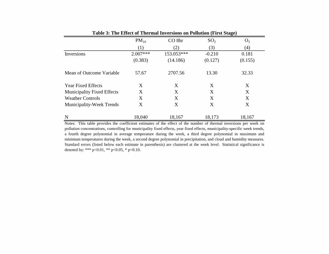
PM10 CO 8hr SO2 O3

(1) (2) (3) (4)Inversions 2.007*** 153.053*** -0.210 0.181

(0.383) (14.186) (0.127) (0.155)

Mean of Outcome Variable 57.67 2707.56 13.30 32.33

Year Fixed Effects X X X XMunicipality Fixed Effects X X X XWeather Controls X X X XMunicipality-Week Trends X X X X

N 18,040 18,167 18,173 18,167Notes: This table provides the coefficient estimates of the effect of the number of thermal inversions per week onpollution concentrations, controlling for municipality fixed effects, year fixed effects, municipality-specific week trends,a fourth degree polynomial in average temperature during the week, a third degree polynomial in maximum andminimum temperatures during the week, a second degree polynomial in precipitation, and cloud and humidity measures.Standard errors (listed below each estimate in parenthesis) are clustered at the week level. Statistical significance isdenoted by: *** p<0.01, ** p<0.05, * p<0.10.

Table 3: The Effect of Thermal Inversions on Pollution (First Stage)

Neonatal Infant Neonatal Infant(1) (2) (3) (4)

Particulate Matter 24hr avg (PM10) 0.1670 0.0237 0.4486 0.2369*

in µg/m3 (0.2706) (0.0272) (0.9607) (0.1216)

Carbon Monoxide 8hr avg. (CO) 0.0085 -0.0006 0.0068 0.0032**in parts per billion (ppb) (0.0097) (0.0011) (0.0133) (0.0014)

Sulfur Dioxide avg (SO2) 1.4325 0.1034in parts per billion (ppb) (1.2619) (0.1273)

Ozone avg (O3) 1.0400 0.1379in parts per billion (ppb) (1.1511) (0.1147)

Mean of Outcome Variables 295.83 38.21 295.83 38.21

Instrument: Inversions X X

Week Fixed Effects X XYear Fixed Effects X XMunicipality Fixed Effects X X X XWeather Controls X X X XMunicipality-Week Trends X X X X

Fixed Effects Instrumental VariablesTable 4: The Effect of Pollution on Infant Mortality

Notes: This table presents Fixed Effects and Instrumental Variable estimates of the effect of pollution on infant mortality.Each coefficient corresponds to a separate regression. The fixed effects estimation, reported in Columns (1) and (2),includes week fixed effects, municipality fixed effects, municipality-specific week trends and weather controls. In theInstrumental Variables estimation, presented in Columns (3) and (4), the number of thermal inversions per week is theexcluded instrument; this model includes year fixed effects, municipality fixed effects, municipality-specific week trends andweather controls. Weather controls are a fourth degree polynomial in average temperature during the week, a third degreepolynomial in maximum and minimum temperatures during the week, a second degree polynomial in precipitation, andcloud and humidity measures. Standard errors (listed below each estimate in parenthesis) are clustered at the week level.Statistical significance is denoted by: *** p<0.01, ** p<0.05, * p<0.10.

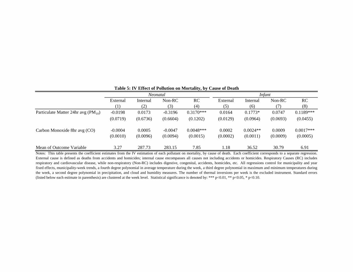
External Internal Non-RC RC External Internal Non-RC RC(1) (2) (3) (4) (5) (6) (7) (8)

Particulate Matter 24hr avg (PM10) -0.0198 0.0173 -0.3196 0.3170*** 0.0164 0.1773* 0.0747 0.1189***

(0.0719) (0.6736) (0.6604) (0.1202) (0.0129) (0.0964) (0.0693) (0.0455)

Carbon Monoxide 8hr avg (CO) -0.0004 0.0005 -0.0047 0.0048*** 0.0002 0.0024** 0.0009 0.0017***(0.0010) (0.0096) (0.0094) (0.0015) (0.0002) (0.0011) (0.0009) (0.0005)

Mean of Outcome Variable 3.27 287.73 283.15 7.85 1.18 36.52 30.79 6.91

InfantNeonatalTable 5: IV Effect of Pollution on Mortality, by Cause of Death

Notes: This table presents the coefficient estimates from the IV estimation of each pollutant on mortality, by cause of death. Each coefficient corresponds to a separate regression.External cause is defined as deaths from accidents and homicides; internal cause encompasses all causes not including accidents or homicides. Respiratory Causes (RC) includesrespiratory and cardiovascular disease, while non-respiratory (Non-RC) includes digestive, congenital, accidents, homicides, etc. All regressions control for municipality and yearfixed effects, municipality-week trends, a fourth degree polynomial in average temperature during the week, a third degree polynomial in maximum and minimum temperatures duringthe week, a second degree polynomial in precipitation, and cloud and humidity measures. The number of thermal inversions per week is the excluded instrument. Standard errors(listed below each estimate in parenthesis) are clustered at the week level. Statistical significance is denoted by: *** p<0.01, ** p<0.05, * p<0.10.

Neonatal Infant

Change in Pollution between

1997 and 2006

Change in infant death rate per year between 1997 and

2006(1) (2) (3) (4)

Particulate Matter 24 hr avg (PM10) -1.6329 0.0696 -21.87 -79.2

(2.2139) (0.2105)

Carbon Monoxide 8hr avg (CO) 0.0293 0.0024 -1581.73 -197.4(0.0324) (0.0032)

Chi2 Stat Joint Significance Test 0.872 5.600 -276.6p-value 0.647 0.0608Notes: Each column in this table presents the results of a single specification that includes CO and PM10 simultaneously. We present the results

of an IV estimation of the multivariate pollution model, where inversions, inversions × altitude, and inversions × thickness are instruments forCO and PM10 (the first stage is reported in Appendix Table 7). Coefficients can be interpreted as the effect of each pollutant, conditional on

the other pollutant. All regressions control for municipality and year fixed effects, municipality-week trends, a fourth degree polynomial inaverage temperature during the week, a third degree polynomial in maximum and minimum temperatures during the week, a second degreepolynomial in precipitation, and cloud and humidity measures. Statistical significance is denoted by: *** p<0.01, ** p<0.05, * p<0.10. Forease of interpretation, in Columns (3) and (4), we calculate the change in infant deaths per year that can be attributed to the change in pollutionin Mexico City between 1997 and 2006 (assuming 282,000 births per year).

Table 6: Multiple Pollutant Models

Neonatal Infant(1) (2)

PM10 max 24hr between 0 and 54.203 and ug/m3 -0.2047 0.2171(2.7675) (0.3297)

PM10 max 24hr between 54.203 and 300 ug/m3 1.5173 0.3219**(1.1804) (0.1449)

Angrist-Pischke F-statistic, First Stage 1 7.247 7.346Angrist-Pischke F-statistic, First Stage 2 9.906 0.001Stock-Yogo weak ID critical value for single endogenous regressor 8.68 8.68

Equal Slopes F (Chi-squared) Statistic 0.365 0.0883p-value 0.546 0.766

CO 8hr avg. between 0 and 3167 ppb -0.0159 0.0001(0.0305) (0.0032)

CO 8hr avg. higher than 3167 ppb 0.0558 0.0082*(0.0422) (0.0047)

Angrist-Pischke F-statistic, First Stage 1 12.17 14.34Angrist-Pischke F-statistic, First Stage 2 14.09 11.58Stock-Yogo weak ID critical value for single endogenous regressor 8.68 8.68

Equal Slopes F (Chi-squared) Statistic 1.152 1.255p-value 0.283 0.263Notes: In this table, we explore whether there is a non-linearity in the dose-response relationship between pollution andmortality. Each column within each panel corresponds to a separate regression. We include a linear spline in bothpollutants to capture the effect of pollution at levels within the range of California's pollution levels in the period used forCurrie and Neidell's (2005) study and the effect at the higher pollution levels observed in many developing countries.Regressions are using 2SLS and include all controls as listed in Table 4. The instrument set consists of three indicatorvariables denoting one thermal inversion, two to three thermal inversions and four to seven thermal inversions during theweek. For ease of interpretation, we include a test for equal slopes to test whether the effect of pollution on mortalitydiffers at low versus high levels. We also report the Angrist-Piscke F-statistic to assess the strength of each of the twofirst stage equations in the model. These statistics should be above the Stock-Yogo critical value for a single endogenousregressor reported below them in order to rule out more than 10% bias due to weak instruments. Standard errors (listedbelow each estimate in parenthesis) are clustered at the week level. Statistical significance is denoted by: *** p<0.01, **p<0.05, * p<0.10.

Table 7: Non-Linearities

Panel A: Linear Spline in PM 10

Panel B: Linear Spline in CO

Infant Mortality Rate Mean Level

Effect Size (Year) Elasticity Mean Level

Effect Size (Year) Elasticity

(1) (2) (3) (4) (5) (6) (7)

Infant Mortality 1986.82 2.71 166.4** 0.227 66.94 12.3188* 0.415Infant Mortality-Internal 1898.85 2.71 124.8** 0.178 66.94 9.2196* 0.325

Currie and Neidell (2005) 391 2.00 16.501** 0.084 39.45 0.013 0.001Currie, Neidell, and Schmieder (2009) 688 1.58 17.6*** 0.040 29.60 -0.189 -0.008Chay and Greenstone (2003) 1179 35.33 9.47** 0.284Knittel, Miller, and Sanders (2011) 280 1.01 40.56 0.146 28.94 17.68** 1.827Notes: In this table, we compare our primary estimates with estimates derived from the United States context. We convert Chay and Greenstone from total suspendedparticulars to particulate matter for ease of comparison. We also provide the elasticity of the infant mortality rate to pollution (Columns 4 and 7). Given that Currie,Neidell, and Schmieder (2009) does not have a directly comparable group, we report their estimates for the 0-2 week age group.

Table 8: Comparison with Literature in United States Setting (Sample for 1 year olds)CO Particulate Matter

Panel A: Mexico City Data

Panel B: Estimates from United States Setting

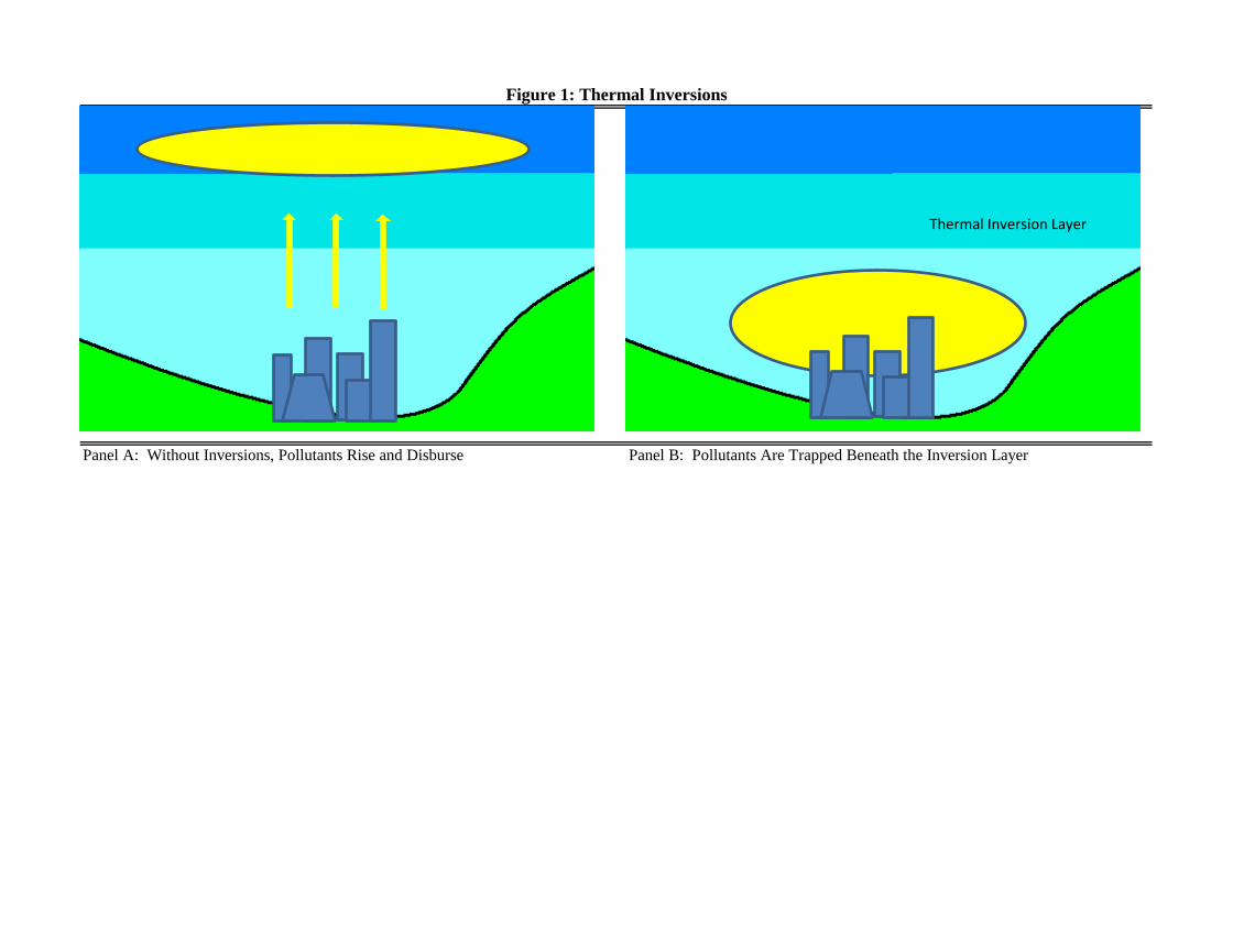
Panel A: Without Inversions, Pollutants Rise and Disburse Panel B: Pollutants Are Trapped Beneath the Inversion Layer

Figure 1: Thermal Inversions

Thermal Inversion Layer

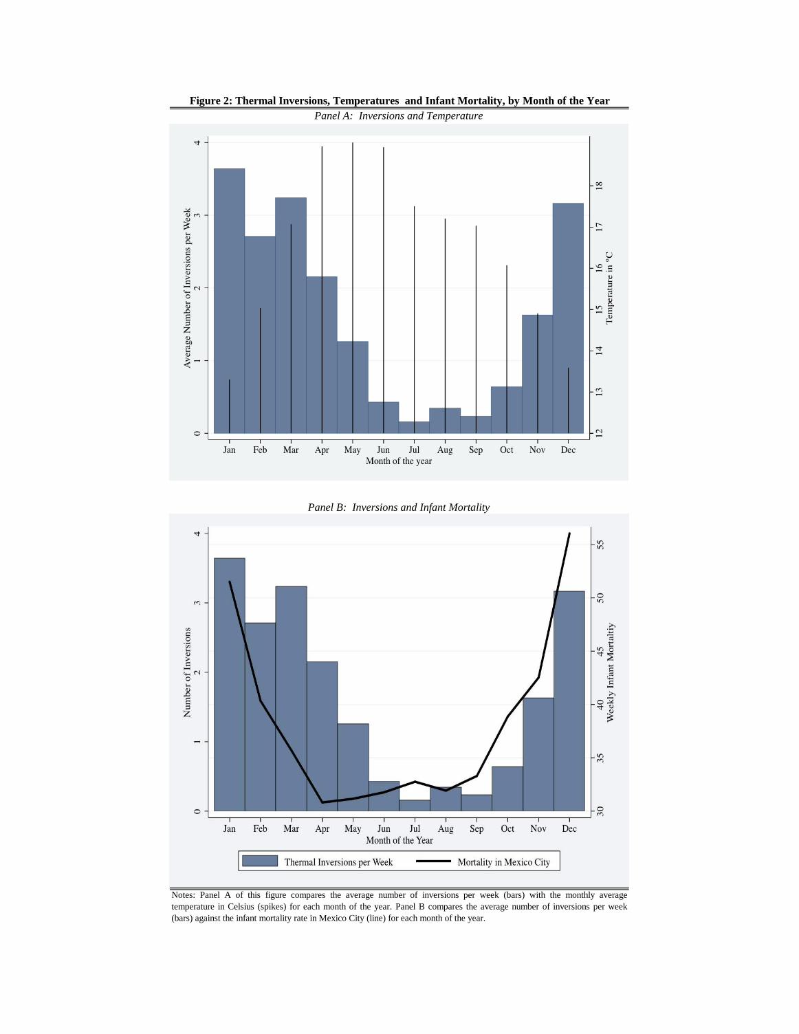
Figure 2: Thermal Inversions, Temperatures and Infant Mortality, by Month of the Year

Notes: Panel A of this figure compares the average number of inversions per week (bars) with the monthly averagetemperature in Celsius (spikes) for each month of the year. Panel B compares the average number of inversions per week(bars) against the infant mortality rate in Mexico City (line) for each month of the year.

Panel A: Inversions and Temperature

Panel B: Inversions and Infant Mortality

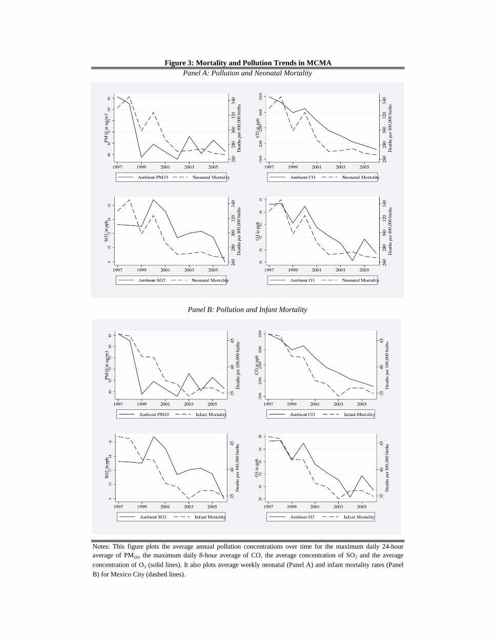
Figure 3: Mortality and Pollution Trends in MCMA

Panel B: Pollution and Infant Mortality

Panel A: Pollution and Neonatal Mortality

Notes: This figure plots the average annual pollution concentrations over time for the maximum daily 24-houraverage of PM10, the maximum daily 8-hour average of CO, the average concentration of SO2 and the average

concentration of O3 (solid lines). It also plots average weekly neonatal (Panel A) and infant mortality rates (Panel

B) for Mexico City (dashed lines).

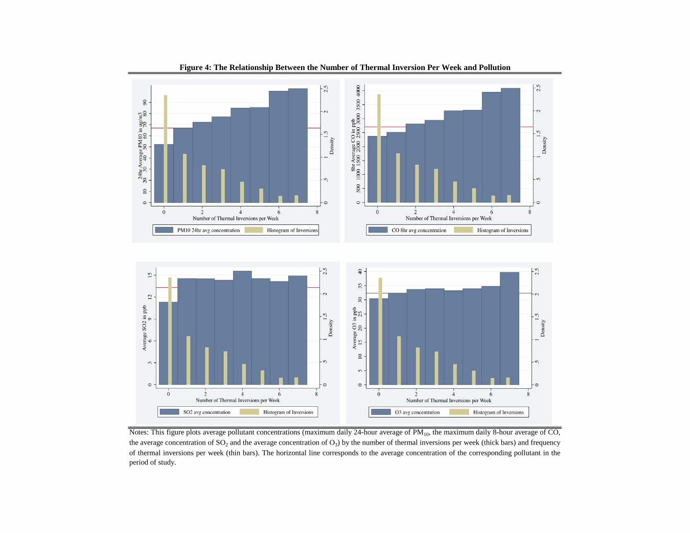
Figure 4: The Relationship Between the Number of Thermal Inversion Per Week and Pollution

Notes: This figure plots average pollutant concentrations (maximum daily 24-hour average of PM10, the maximum daily 8-hour average of CO,the average concentration of SO2 and the average concentration of O3) by the number of thermal inversions per week (thick bars) and frequencyof thermal inversions per week (thin bars). The horizontal line corresponds to the average concentration of the corresponding pollutant in theperiod of study.

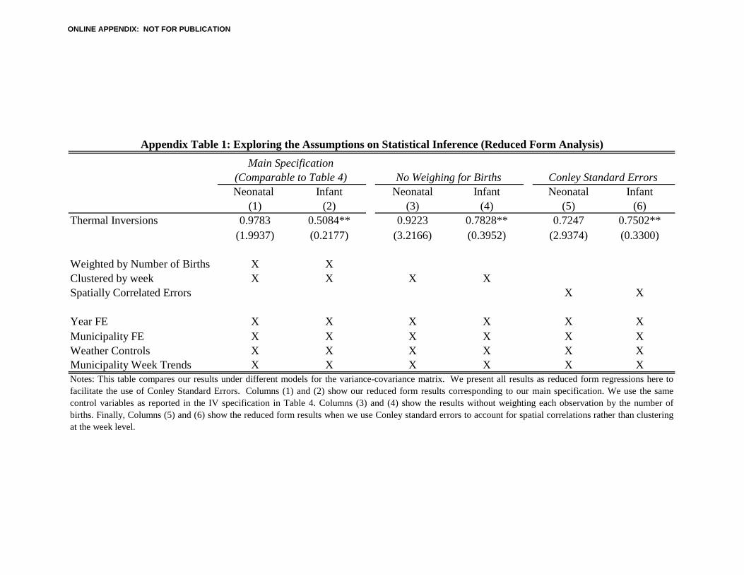
Neonatal Infant Neonatal Infant Neonatal Infant(1) (2) (3) (4) (5) (6)

Thermal Inversions 0.9783 0.5084** 0.9223 0.7828** 0.7247 0.7502**(1.9937) (0.2177) (3.2166) (0.3952) (2.9374) (0.3300)

Weighted by Number of Births X XClustered by week X X X XSpatially Correlated Errors X X

Year FE X X X X X XMunicipality FE X X X X X XWeather Controls X X X X X XMunicipality Week Trends X X X X X X

Appendix Table 1: Exploring the Assumptions on Statistical Inference (Reduced Form Analysis)

Main Specification (Comparable to Table 4) No Weighing for Births Conley Standard Errors

Notes: This table compares our results under different models for the variance-covariance matrix. We present all results as reduced form regressions here tofacilitate the use of Conley Standard Errors. Columns (1) and (2) show our reduced form results corresponding to our main specification. We use the samecontrol variables as reported in the IV specification in Table 4. Columns (3) and (4) show the results without weighting each observation by the number ofbirths. Finally, Columns (5) and (6) show the reduced form results when we use Conley standard errors to account for spatial correlations rather than clusteringat the week level.

ONLINE APPENDIX: NOT FOR PUBLICATION

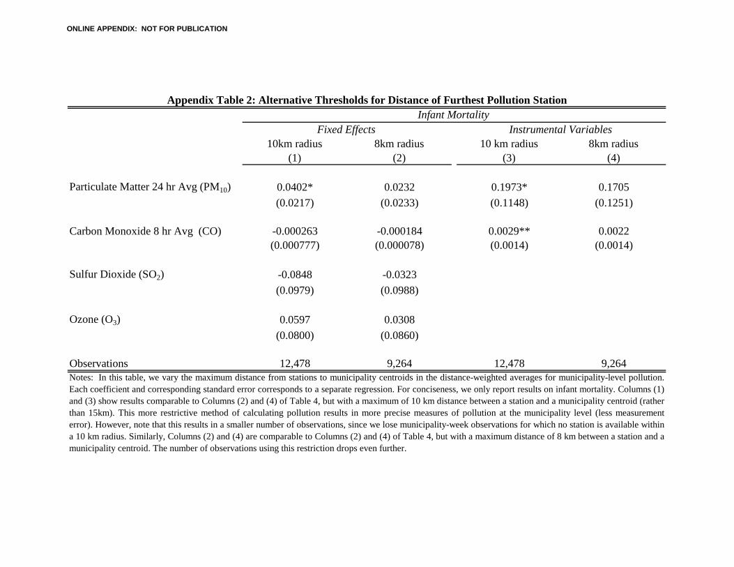
10km radius 8km radius 10 km radius 8km radius(1) (2) (3) (4)

Particulate Matter 24 hr Avg (PM10) 0.0402* 0.0232 0.1973* 0.1705(0.0217) (0.0233) (0.1148) (0.1251)

Carbon Monoxide 8 hr Avg (CO) -0.000263 -0.000184 0.0029** 0.0022(0.000777) (0.000078) (0.0014) (0.0014)

Sulfur Dioxide (SO2) -0.0848 -0.0323(0.0979) (0.0988)

Ozone (O3) 0.0597 0.0308(0.0800) (0.0860)

Observations 12,478 9,264 12,478 9,264

Instrumental Variables

Appendix Table 2: Alternative Thresholds for Distance of Furthest Pollution Station

Fixed Effects

Notes: In this table, we vary the maximum distance from stations to municipality centroids in the distance-weighted averages for municipality-level pollution.Each coefficient and corresponding standard error corresponds to a separate regression. For conciseness, we only report results on infant mortality. Columns (1)and (3) show results comparable to Columns (2) and (4) of Table 4, but with a maximum of 10 km distance between a station and a municipality centroid (ratherthan 15km). This more restrictive method of calculating pollution results in more precise measures of pollution at the municipality level (less measurementerror). However, note that this results in a smaller number of observations, since we lose municipality-week observations for which no station is available withina 10 km radius. Similarly, Columns (2) and (4) are comparable to Columns (2) and (4) of Table 4, but with a maximum distance of 8 km between a station and amunicipality centroid. The number of observations using this restriction drops even further.

Infant Mortality

ONLINE APPENDIX: NOT FOR PUBLICATION

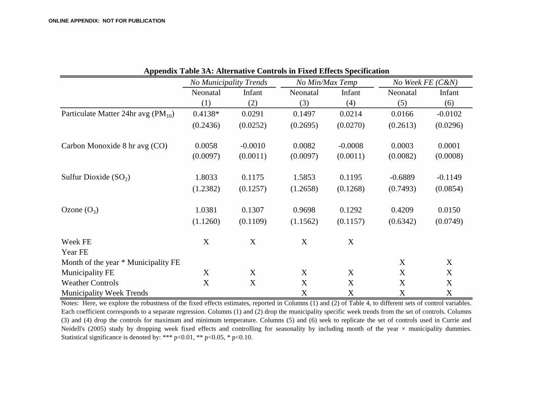
Neonatal Infant Neonatal Infant Neonatal Infant(1) (2) (3) (4) (5) (6)

Particulate Matter 24hr avg (PM10) 0.4138* 0.0291 0.1497 0.0214 0.0166 -0.0102(0.2436) (0.0252) (0.2695) (0.0270) (0.2613) (0.0296)

Carbon Monoxide 8 hr avg (CO) 0.0058 -0.0010 0.0082 -0.0008 0.0003 0.0001(0.0097) (0.0011) (0.0097) (0.0011) (0.0082) (0.0008)

Sulfur Dioxide (SO2) 1.8033 0.1175 1.5853 0.1195 -0.6889 -0.1149(1.2382) (0.1257) (1.2658) (0.1268) (0.7493) (0.0854)

Ozone (O3) 1.0381 0.1307 0.9698 0.1292 0.4209 0.0150(1.1260) (0.1109) (1.1562) (0.1157) (0.6342) (0.0749)

Week FE X X X XYear FEMonth of the year * Municipality FE X XMunicipality FE X X X X X XWeather Controls X X X X X XMunicipality Week Trends X X X X

Appendix Table 3A: Alternative Controls in Fixed Effects Specification

Notes: Here, we explore the robustness of the fixed effects estimates, reported in Columns (1) and (2) of Table 4, to different sets of control variables.Each coefficient corresponds to a separate regression. Columns (1) and (2) drop the municipality specific week trends from the set of controls. Columns(3) and (4) drop the controls for maximum and minimum temperature. Columns (5) and (6) seek to replicate the set of controls used in Currie andNeidell's (2005) study by dropping week fixed effects and controlling for seasonality by including month of the year × municipality dummies.Statistical significance is denoted by: *** p<0.01, ** p<0.05, * p<0.10.

No Municipality Trends No Min/Max Temp No Week FE (C&N)

ONLINE APPENDIX: NOT FOR PUBLICATION

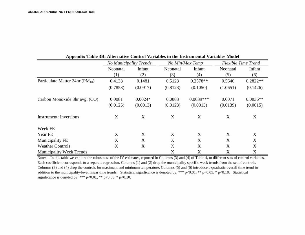
Neonatal Infant Neonatal Infant Neonatal Infant(1) (2) (3) (4) (5) (6)

Particulate Matter 24hr (PM10) 0.4133 0.1481 0.5123 0.2578** 0.5640 0.2822**(0.7853) (0.0917) (0.8123) (0.1050) (1.0651) (0.1426)

Carbon Monoxide 8hr avg. (CO) 0.0081 0.0024* 0.0083 0.0039*** 0.0071 0.0036**(0.0125) (0.0013) (0.0123) (0.0013) (0.0139) (0.0015)

Instrument: Inversions X X X X X X

Week FEYear FE X X X X X XMunicipality FE X X X X X XWeather Controls X X X X X XMunicipality Week Trends X X X XNotes: In this table we explore the robustness of the IV estimates, reported in Columns (3) and (4) of Table 4, to different sets of control variables. Each coefficient corresponds to a separate regression. Columns (1) and (2) drop the municipality specific week trends from the set of controls. Columns (3) and (4) drop the controls for maximum and minimum temperature. Columns (5) and (6) introduce a quadratic overall time trend in addition to the municipality-level linear time trends. Statistical significance is denoted by: *** p<0.01, ** p<0.05, * p<0.10. Statistical significance is denoted by: *** p<0.01, ** p<0.05, * p<0.10.

Appendix Table 3B: Alternative Control Variables in the Instrumental Variables ModelNo Municipality Trends No Min/Max Temp Flexible Time Trend

ONLINE APPENDIX: NOT FOR PUBLICATION

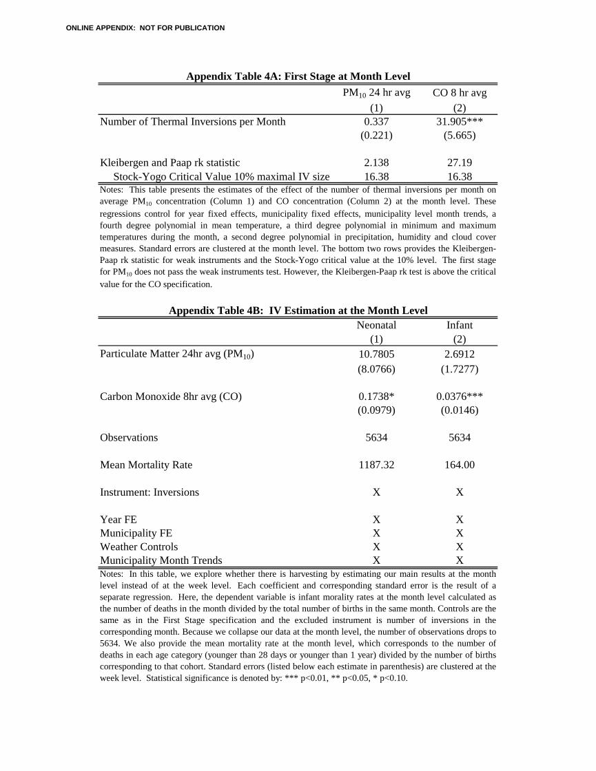
PM10 24 hr avg CO 8 hr avg(1) (2)

Number of Thermal Inversions per Month 0.337 31.905***(0.221) (5.665)

Kleibergen and Paap rk statistic 2.138 27.19Stock-Yogo Critical Value 10% maximal IV size 16.38 16.38

Neonatal Infant(1) (2)

Particulate Matter 24hr avg (PM10) 10.7805 2.6912(8.0766) (1.7277)

Carbon Monoxide 8hr avg (CO) 0.1738* 0.0376***(0.0979) (0.0146)

Observations 5634 5634

Mean Mortality Rate 1187.32 164.00

Instrument: Inversions X X

Year FE X XMunicipality FE X XWeather Controls X XMunicipality Month Trends X X

Appendix Table 4B: IV Estimation at the Month Level

Appendix Table 4A: First Stage at Month Level

Notes: In this table, we explore whether there is harvesting by estimating our main results at the monthlevel instead of at the week level. Each coefficient and corresponding standard error is the result of aseparate regression. Here, the dependent variable is infant morality rates at the month level calculated asthe number of deaths in the month divided by the total number of births in the same month. Controls are thesame as in the First Stage specification and the excluded instrument is number of inversions in thecorresponding month. Because we collapse our data at the month level, the number of observations drops to5634. We also provide the mean mortality rate at the month level, which corresponds to the number ofdeaths in each age category (younger than 28 days or younger than 1 year) divided by the number of birthscorresponding to that cohort. Standard errors (listed below each estimate in parenthesis) are clustered at theweek level. Statistical significance is denoted by: *** p<0.01, ** p<0.05, * p<0.10.

Notes: This table presents the estimates of the effect of the number of thermal inversions per month onaverage PM10 concentration (Column 1) and CO concentration (Column 2) at the month level. Theseregressions control for year fixed effects, municipality fixed effects, municipality level month trends, afourth degree polynomial in mean temperature, a third degree polynomial in minimum and maximumtemperatures during the month, a second degree polynomial in precipitation, humidity and cloud covermeasures. Standard errors are clustered at the month level. The bottom two rows provides the Kleibergen-Paap rk statistic for weak instruments and the Stock-Yogo critical value at the 10% level. The first stagefor PM10 does not pass the weak instruments test. However, the Kleibergen-Paap rk test is above the criticalvalue for the CO specification.

ONLINE APPENDIX: NOT FOR PUBLICATION

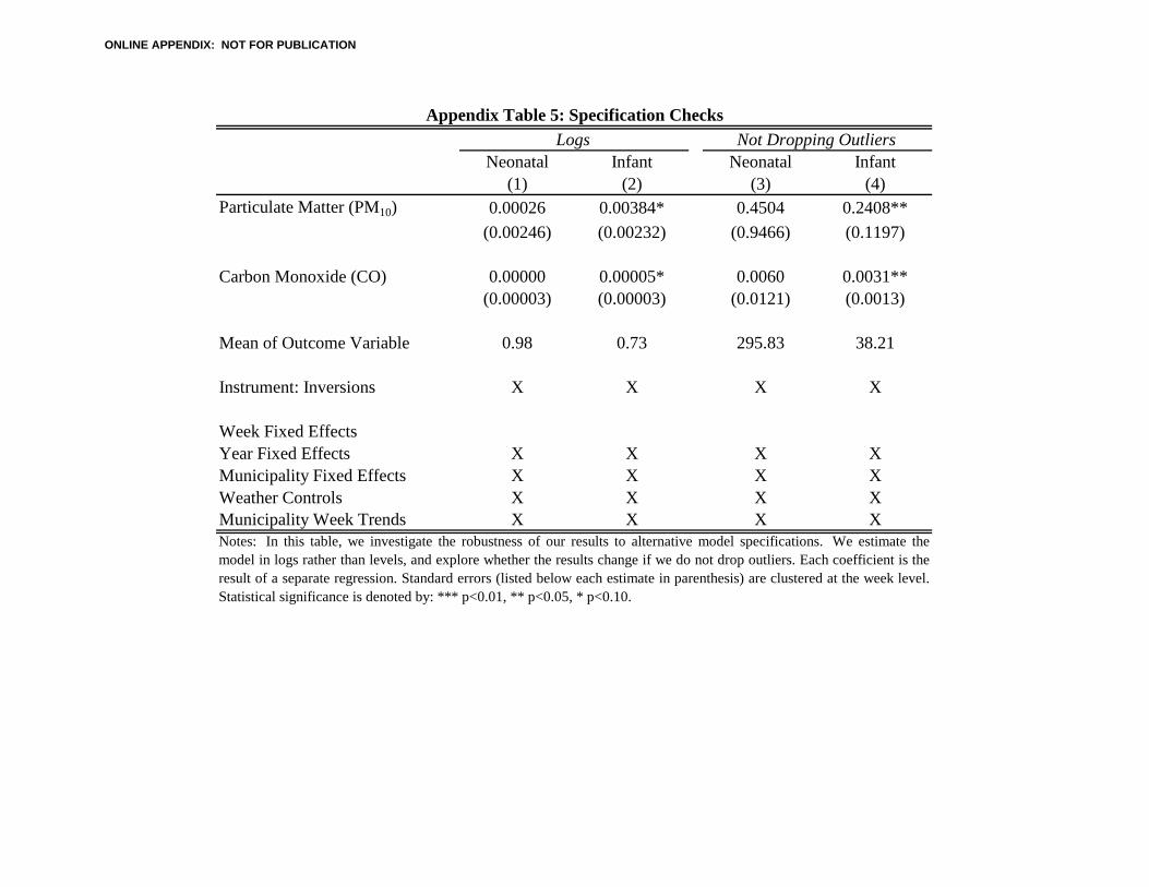
Neonatal Infant Neonatal Infant(1) (2) (3) (4)

Particulate Matter (PM10) 0.00026 0.00384* 0.4504 0.2408**(0.00246) (0.00232) (0.9466) (0.1197)

Carbon Monoxide (CO) 0.00000 0.00005* 0.0060 0.0031**(0.00003) (0.00003) (0.0121) (0.0013)

Mean of Outcome Variable 0.98 0.73 295.83 38.21

Instrument: Inversions X X X X

Week Fixed EffectsYear Fixed Effects X X X XMunicipality Fixed Effects X X X XWeather Controls X X X XMunicipality Week Trends X X X X

Logs Not Dropping OutliersAppendix Table 5: Specification Checks

Notes: In this table, we investigate the robustness of our results to alternative model specifications. We estimate themodel in logs rather than levels, and explore whether the results change if we do not drop outliers. Each coefficient is theresult of a separate regression. Standard errors (listed below each estimate in parenthesis) are clustered at the week level.Statistical significance is denoted by: *** p<0.01, ** p<0.05, * p<0.10.

ONLINE APPENDIX: NOT FOR PUBLICATION

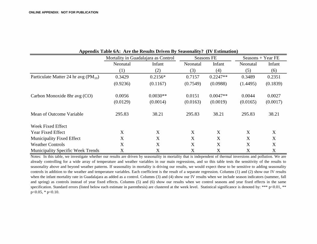
Neonatal Infant Neonatal Infant Neonatal Infant(1) (2) (3) (4) (5) (6)

Particulate Matter 24 hr avg (PM10) 0.3429 0.2156* 0.7157 0.2247** 0.3489 0.2351(0.9236) (0.1167) (0.7549) (0.0988) (1.4495) (0.1839)

Carbon Monoxide 8hr avg (CO) 0.0056 0.0030** 0.0151 0.0047** 0.0044 0.0027(0.0129) (0.0014) (0.0163) (0.0019) (0.0165) (0.0017)

Mean of Outcome Variable 295.83 38.21 295.83 38.21 295.83 38.21

Week Fixed EffectYear Fixed Effect X X X X X XMunicipality Fixed Effect X X X X X XWeather Controls X X X X X XMunicipality Specific Week Trends X X X X X X

Mortality in Guadalajara as Control Seasons FE Seasons + Year FEAppendix Table 6A: Are the Results Driven By Seasonality? (IV Estimation)

Notes: In this table, we investigate whether our results are driven by seasonality in mortality that is independent of thermal inversions and pollution. We arealready controlling for a wide array of temperature and weather variables in our main regressions, and so this table tests the sensitivity of the results toseasonality above and beyond weather patterns. If seasonality in mortality is driving our results, we would expect these to be sensitive to adding seasonalitycontrols in addition to the weather and temperature variables. Each coefficient is the result of a separate regression. Columns (1) and (2) show our IV resultswhen the infant mortality rate in Guadalajara as added as a control. Columns (3) and (4) show our IV results when we include season indicators (summer, falland spring) as controls instead of year fixed effects. Columns (5) and (6) show our results when we control seasons and year fixed effects in the samespecification. Standard errors (listed below each estimate in parenthesis) are clustered at the week level. Statistical significance is denoted by: *** p<0.01, **p<0.05, * p<0.10.

ONLINE APPENDIX: NOT FOR PUBLICATION

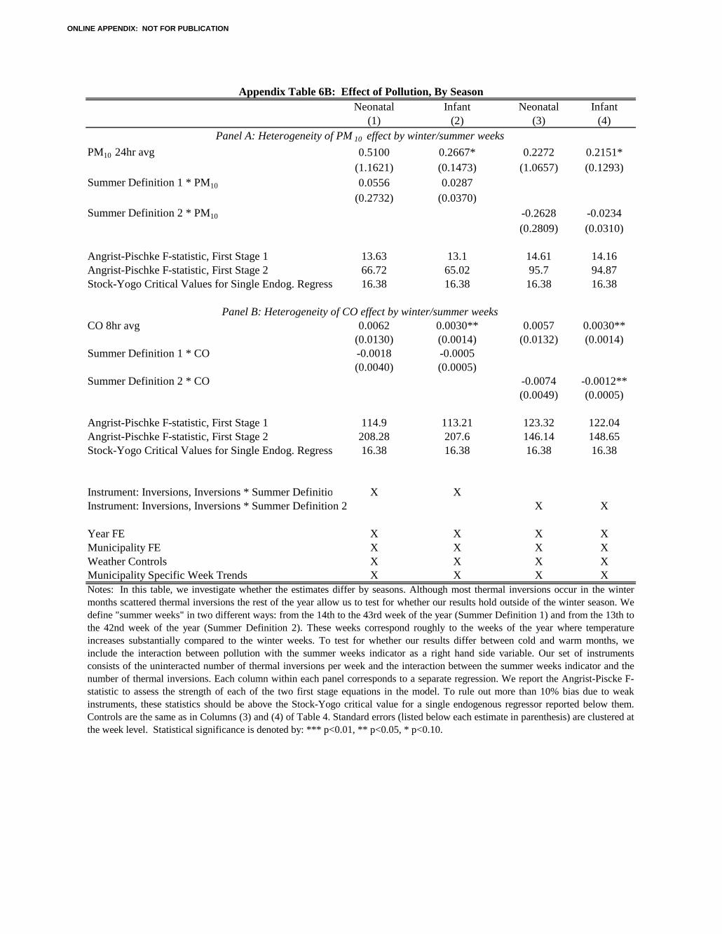
Neonatal Infant Neonatal Infant(1) (2) (3) (4)

PM10 24hr avg 0.5100 0.2667* 0.2272 0.2151*(1.1621) (0.1473) (1.0657) (0.1293)

Summer Definition 1 * PM10 0.0556 0.0287(0.2732) (0.0370)

Summer Definition 2 * PM10 -0.2628 -0.0234(0.2809) (0.0310)

Angrist-Pischke F-statistic, First Stage 1 13.63 13.1 14.61 14.16Angrist-Pischke F-statistic, First Stage 2 66.72 65.02 95.7 94.87Stock-Yogo Critical Values for Single Endog. Regress 16.38 16.38 16.38 16.38

CO 8hr avg 0.0062 0.0030** 0.0057 0.0030**(0.0130) (0.0014) (0.0132) (0.0014)

Summer Definition 1 * CO -0.0018 -0.0005(0.0040) (0.0005)

Summer Definition 2 * CO -0.0074 -0.0012**(0.0049) (0.0005)

Angrist-Pischke F-statistic, First Stage 1 114.9 113.21 123.32 122.04Angrist-Pischke F-statistic, First Stage 2 208.28 207.6 146.14 148.65Stock-Yogo Critical Values for Single Endog. Regress 16.38 16.38 16.38 16.38

Instrument: Inversions, Inversions * Summer Definitio X XInstrument: Inversions, Inversions * Summer Definition 2 X X

Year FE X X X XMunicipality FE X X X XWeather Controls X X X XMunicipality Specific Week Trends X X X X

Appendix Table 6B: Effect of Pollution, By Season

Notes: In this table, we investigate whether the estimates differ by seasons. Although most thermal inversions occur in the wintermonths scattered thermal inversions the rest of the year allow us to test for whether our results hold outside of the winter season. Wedefine "summer weeks" in two different ways: from the 14th to the 43rd week of the year (Summer Definition 1) and from the 13th tothe 42nd week of the year (Summer Definition 2). These weeks correspond roughly to the weeks of the year where temperatureincreases substantially compared to the winter weeks. To test for whether our results differ between cold and warm months, weinclude the interaction between pollution with the summer weeks indicator as a right hand side variable. Our set of instrumentsconsists of the uninteracted number of thermal inversions per week and the interaction between the summer weeks indicator and thenumber of thermal inversions. Each column within each panel corresponds to a separate regression. We report the Angrist-Piscke F-statistic to assess the strength of each of the two first stage equations in the model. To rule out more than 10% bias due to weakinstruments, these statistics should be above the Stock-Yogo critical value for a single endogenous regressor reported below them.Controls are the same as in Columns (3) and (4) of Table 4. Standard errors (listed below each estimate in parenthesis) are clustered atthe week level. Statistical significance is denoted by: *** p<0.01, ** p<0.05, * p<0.10.

Panel B: Heterogeneity of CO effect by winter/summer weeks

Panel A: Heterogeneity of PM 10 effect by winter/summer weeks

ONLINE APPENDIX: NOT FOR PUBLICATION

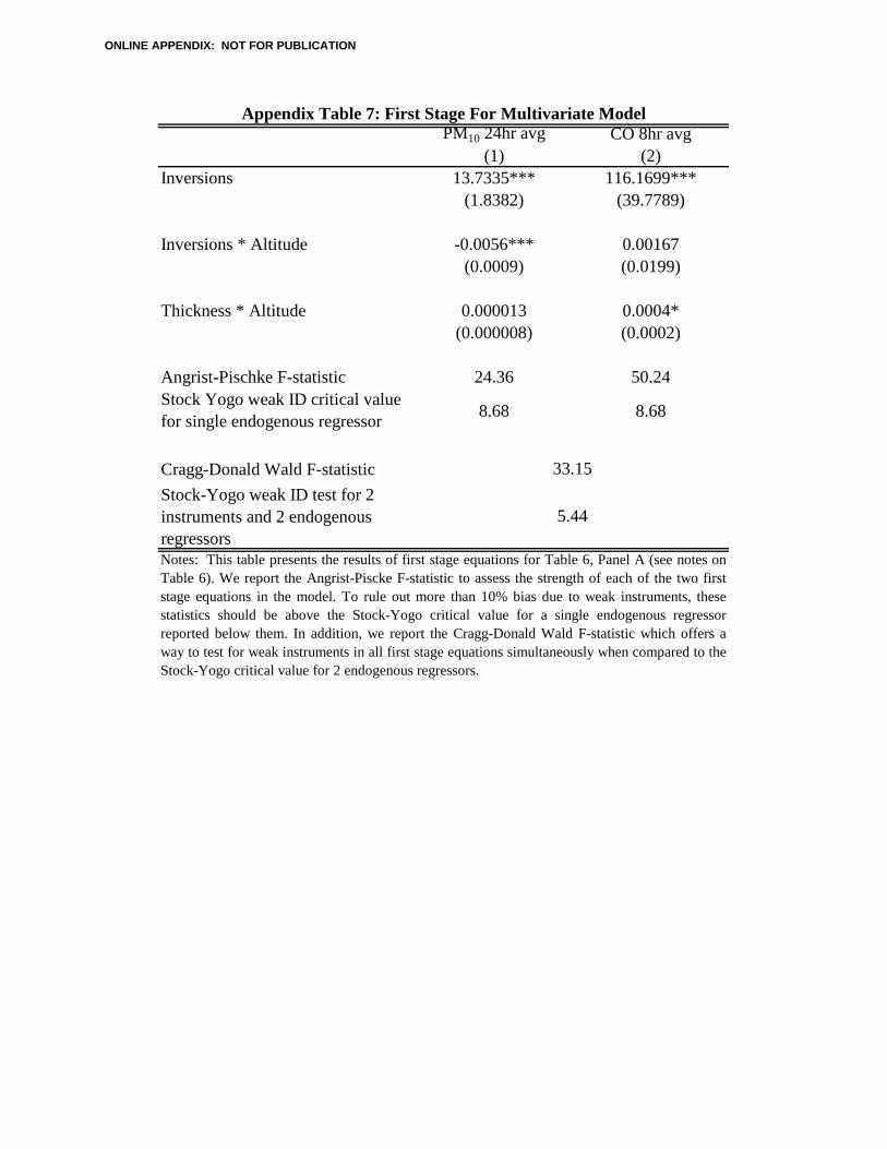
PM10 24hr avg CO 8hr avg(1) (2)

Inversions 13.7335*** 116.1699***(1.8382) (39.7789)

Inversions * Altitude -0.0056*** 0.00167(0.0009) (0.0199)

Thickness * Altitude 0.000013 0.0004*(0.000008) (0.0002)

Angrist-Pischke F-statistic 24.36 50.24Stock Yogo weak ID critical value for single endogenous regressor 8.68 8.68

Cragg-Donald Wald F-statisticStock-Yogo weak ID test for 2 instruments and 2 endogenous regressors

Appendix Table 7: First Stage For Multivariate Model

Notes: This table presents the results of first stage equations for Table 6, Panel A (see notes onTable 6). We report the Angrist-Piscke F-statistic to assess the strength of each of the two firststage equations in the model. To rule out more than 10% bias due to weak instruments, thesestatistics should be above the Stock-Yogo critical value for a single endogenous regressorreported below them. In addition, we report the Cragg-Donald Wald F-statistic which offers away to test for weak instruments in all first stage equations simultaneously when compared to theStock-Yogo critical value for 2 endogenous regressors.

33.15

5.44

ONLINE APPENDIX: NOT FOR PUBLICATION

Infant Mortality Rate Mean Level Effect Size

(Year) Elasticity Mean Level Effect Size (Year) Elasticity

(1) (2) (3) (4) (5) (6) (7)

Infant Mortality 1986.82 2.70756 124.8 0.170 66.94 3.6192 0.120

Currie and Neidell (2005) 391 1.998 18.125** 0.093 39.448 -0.226 -0.024Knittel, Miller, and Sanders (2011 280 1.01 80.6 0.291 28.94 18.2*** 1.881Notes: This table replicates Table 8 but uses the estimates from the multiple regression model rather than the single regression models.

Appendix Table 8: Comparison with Literature in United States Setting (Multiple Regression Results)CO Particulate Matter

Panel A: Mexico City Data

Panel B: Estimates from United States Setting

ONLINE APPENDIX: NOT FOR PUBLICATION

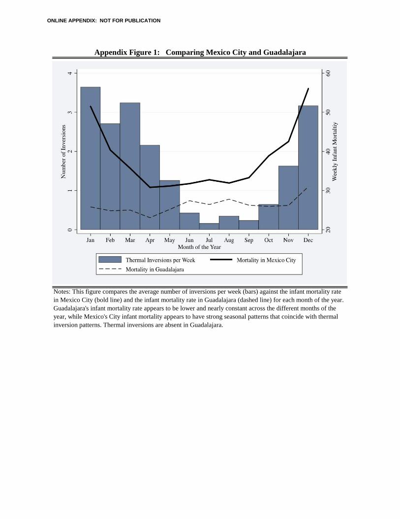
Appendix Figure 1: Comparing Mexico City and Guadalajara

Notes: This figure compares the average number of inversions per week (bars) against the infant mortality rate in Mexico City (bold line) and the infant mortality rate in Guadalajara (dashed line) for each month of the year. Guadalajara's infant mortality rate appears to be lower and nearly constant across the different months of the year, while Mexico's City infant mortality appears to have strong seasonal patterns that coincide with thermal inversion patterns. Thermal inversions are absent in Guadalajara.

ONLINE APPENDIX: NOT FOR PUBLICATION