Does the waterbed effect harm consumers?PRELIMINARY VERSION, PLEASE DO NOT QUOTE

Tommaso Majer

December 5, 2008

Departament d’Economia i d’Historia Economica, Edifici B

Universitat Autonoma de Barcelona

08193 Bellaterra (Barcelona), Spain

Abstract

In this paper I analyse how the exercise of buyer power can raise the

price of the wholesale good of the rival firms (the so-called waterbed

effect). In particular, I consider an economy with two markets: in the

first one, the wholesale market, an upstream firm sells an intermediate

good to two downstream firms. These firms use the input to produce

a final good that they sell to the consumers in the second market,

the final consumption market. The price of the intermediate good is

the outcome of simultaneous and independent negotiations between

the upstream and each downstream firm. I consider a setting with

asymmetric negotiations where a change of the bargaining power of

one of the two downstream firms provoques the waterbed effect.The

main contribution of the paper is the fact that I allow for any possible

distribution of bargaining power between the two parties and that the

value of the outside option of each part is endogenous. Furthermore, I

analyze the welfare consequences and I show how the intensity of the

downstream competition affects the existence of such effect.

1

1 Introduction

Usually a good reaches the final consumer after passing through many inter-

mediaries and distributors, and at each of these levels of distribution, buyers

and sellers determine the price of the product. However, until recent times,

economists have paid little attention to these intermediary steps and didn’t

focus their attention to these retailing and distribution activities. The tra-

ditional vision of a market when a unique price for input is fixed may not

be appropriate to describe such trade relations. For example, recently the

United Kingdom Competition Commission attempted to investigate these

kind of relashionships in the inquiry [19] into the grocery retailing sector.

One part of this investigation was about the complaints of small distributors

against the price manipulation induced by the large distributor chains. The

formers complained that the discount obtained by the latters (in particular

Tesco) resulted in higher supplier prices for the small grocery retailers.

This inquiry driven by the Competition Commission analyzing these com-

plaints, led to coin the term “waterbed effect”. To have an intuition of that,

imagine two people seated on a bed made of water. If one person puts on

weight he goes down because he becomes heavier and the other person goes

up, even if he doesn’t put on weight.

In the same way one firm when becomes larger or, in a wider sense, more

powerful, may lower its wholesale price and this discount may result in a

higher price for the other firms.

To define this effect, consider an economy with several downstream and up-

stream firms. Downstream firms buy an input from upstream firms that is

used to produce a consumption good. The price of such input is the outcome

of a negotiation between an upstream and a downstream firm. The waterbed

effect refers to the phenomenon by which the large downstream firms (in

terms of bargaining power) manages to obtain the input at a discount price.

In turn, this induces a (negative) externality on the smaller downstream firms

(those with low bargaining power) in the form of a higher price of the input.

In the UK grocery market the small distributors claimed that suppliers

overcharged them, because they needed to make up margins lost to the big

distributors. In other words, they claimed that the large retailers obtained a

2

price reduction of the price of the good bought from the suppliers, and that

this discount resulted in an higher price for them. That is, the waterbed

effect occurred.

At first glance, this effect may not be intuitive, because even if a down-

stream firm obtains a discount, it does not imply that the negotiated prices

should change. In fact, if it would possible for the supplier to raise its price

to other downstream firms, the supplier would have already done so.

At the end of the inquiry, the UK Competition Commission didn’t find

evidence of the relashionship between these discounts and the higher prices.

This paper contains an attempt to inquire into the rationale of this phe-

nomenon and here we present a model in which the waterbed effect is a

result of the strategic features of the negotiation processes. This point of

view is supported by some papers that explain how such effect arises from

the interaction of the firms involved in the downstream market and in the

negotiations. The added value of this paper to this literature is to generalize

the distribution of the bargaining power between the firms involved in the

negotiation process and to endogenize the value of the outside options.

We propose a simple framework with one upstream firm and two down-

stream firms in an economy with two markets. In the first one, the wholesale

market, the upstream firm sells an intermediate good to the two downstream

firms. The price of this input for each firm is determined by a simultaneous

and independent negotiation process. In the second market, the consumption

good market, the downstream firms compete for consumers.

The rationale is the following. We argue that if a downstream firm ob-

tains a discount in the price negotiated with the supplier, then this firm can

lower the price of its final good and increase the quantity of good sold in

the final consumption market. The decrease of the input price harms the

upstream firm, that will charge an higher price to the other downstream firm

in order to make the profits it didn’t make in the former negotiation. This

is possible only whether the competition in the downstream market is not

intense. When the downstream competition is intense, then the discount

obtained by the strong downstream firm harms the weak downstream firm

and then the upstream firm can not charge an higher price.

3

2 Literature

2.1 Bargaining

There is a recent literature studying the price formation between suppliers

and retailers using a negotiation mechanisms. Chae and Heidhues in [1]

study the effects of downstream coalitions on the bargaining power of a sin-

gle downstream firm and on the number of varieties that the upstream firm

will supply. They show that the bargaining power of the downstream firms

increases with respect to the bargaining power of the upstream firms and this

lowers the incentives for entry in the upstream production industry. Chae

and Heidhues [2] consider two markets (each one with one supplier and one

retailer) and investigate the effect of buyers’ alliances on the outcome of the

negotiation between the supplier and the retailer to determine the price of

the traded good. They find conditions under which the alliance benefits the

buyers. To solve their problem Chae and Heidhues use the Zeuthen-Nash

solution that extend the Nash solution in two directions: it extends it to

situations where a player bargains with multiple players simultaneously and

to situations where a negotiation party is a coalition of agents.

Inderst and Wey [9] study the incentives for horizontal merger in a model

of multilateral bargaining. In their model there are two suppliers and two

downstream firms. They propose a particular bargaining procedure and they

show that this procedure generates the Shapley value. They investigate the

distribution of the profits of the upstream and downstream firms under differ-

ent industry structures. Furthermore, they study how the horizontal merger

decision changes with different types of technologies. Raskovich [16] presents

a model of ordered bargaining where buyers choose the order in which they

bargain with suppliers of known characteristic. This is different from the

common assumption that meetings between traders are generated randomly.

He presents a static model with a finite number of suppliers with no capacity

constraints. In this model the outside option is determined endogenously

(the outside option was always treated as exogenous). All players have full

information and the game is common knowledge. One party makes a take-it-

or-leave-it-offer.If an offer p is accepted, they trade and the game finishes for

4

the buyer. If the offer is rejected, the two parties don’t trade and the buyers

bargains with another supplier. Raskovich finds that the strategic bargain-

ing outcome is equivalent to the generalized Nash bargaining solution and

he proves that a buyer starts bargain with the supplier that gives him the

expected highest payoff.

Faulı-Oller and Sandonıs [14] analyze the optimal two-part tariff that

a research laboratory should propose to sell a patented innovation to two

downstream firms. The innovation will be used by two firms that produce

differentiated goods. They analyze whether the research laboratory prefers to

sell the innovation or to merge with one of the firms in the downstream indus-

try. These authors [3] also consider one firm willing to transfer technological

knowledge. This firm has two different alternatives: licensing or merging.

They show that when both per-unit price and fixed fees are feasible, merger

should not be allowed.

2.2 Waterbed effect

The literature about the waterbed effect is scarce, probably because people

paid attention to the waterbed effect only after that the UK Competition

Commission started to investigating it.

Inderst and Mazzarotto present a literature survey of models of buyer power

[7]. They define bargaining power as the bargaining strength that a buyer

has with respect to the seller with whom it trades. They presents also a

section on waterbed effect, considered as a consequence of the exercise of

buyer power. They consider a monopolistic supplier producing an input

good at marginal cost k that sells the good at price w. If the supplier has all

the bargaining power and the retailer has no alternative supply sources, the

supplier will choose w to maximize its profits and the retailer chooses p. This

price will exceed the price chosen by a vertical integrated firm. There is the

double marginalization problem. If the supplier’s marginal cost are increasing

this problem is mitigated. If the retailer has all the bargaining power, the

wholesale price w is equal to the marginal cost of the supplier: w = k.

To eliminate the double marginalization problem they could use two-part

tariffs. But such contracts have no impacts on the retail price. Furthermore,

5

if the downstream demand is perfectly elastic, no pass-through to consumers

occur, as no market power could be exerted. If a powerful retailer obtains a

discount that is passed through into lower retail prices, this should benefit

its own customers. Authorities are worried about what such a process would

entail for the future structure of retail market. That is, if this effect could

result in higher concentration and prices when less powerful retailers exit the

market. It may be the case that less powerful retailers don’t lower prices

in response to competition. This could happen if suppliers raise wholesale

prices for the other retailers. One possible argument for the existence of this

waterbed effect can be linked to changes in upstream market. If the suppliers

must decrease the wholesale price, their profits decrease, and may be forced

to exit. The remaining suppliers have more power and can charge an higher

price. The increase of the buyer power can compensate the powerful retailer.

Another possibility is linked to changes in the downstream market. Ma-

jumdar in [11] considers a set-up in which there are two upstream firms and

several downstream firms that operate in different local markets. He shows

that a downstream firm can have an incentive to merge horizontally and that

the wholesale price for the new entity will decrease and the wholesale price

for the other downstream firms will increases. He shows that a merger may

cause the waterbed effect.

Inderst and Valletti [8] present a two stage model where the growth of

one firm causes the waterbed effect. In the second stage two downstream

firms compete in the final consumption market. In the first stage there is

a monopolist that makes a take-it-or-leave-it offer and the retailers decide

whether to accept the offer or switch to another supply source paying a fixed

cost. Finally, they show that with linear demand, low fixed cost and other

conditions, the waterbed effect exists and harms consumers.

Inderst [6] analyzes also how the exercise of buyer power can trigger and

accelerate concentration in the downstream industry. He shows how the ex-

istence of discount induces incentives for the big buyers to grow even further.

Finally, Genakos and Valletti [4] document empirically the existence of the

waterbed effect in the mobile telephony market.

The paper is organized as follows. I present the model and discuss the

assumptions in section 3. I find the conditions such that the waterbed effect

6

arises in a asymmetric bargaining setting in section 4. Section 5 presents the

welfare analysis and section 6 concludes. In the appendix A, I extend the

model and I consider the effects of an increase of the efficiency through a

reduction of the marginal cost.

3 The model

Now we introduce the model and we explain its added value. Consider a

two stage model with two downstream firms D1 and D2 and an upstream

firm U : in the first stage, U sells an intermediate good to D1 and D2. The

equilibrium input prices are determined by a negotiation between U and each

downstream firm. Thus, there are two negotiations and the outcomes will be

two wholesale prices w1 and w2, one for each downstream firm. In the second

stage, D1 and D2 compete in a final homogeneous consumption market and

sell their final good to consumers at a price pi.

U

D1 D2

w2w1

(β)(α)

(1− β)(1− α)

p p

final consumption market

3.1 The negotiations

The solution concept we use to find the price of the input good is that of Nash

bargaining solution. Consider the negotiation between U and Di. Profits of

U are ΠU , derived from selling the input good to both D1 and D2. Its

outside option is ΠifU and represents the profits of U when the negotiation

with Di fails and it sells the input good only to Dj. Furthermore, profits

of Di come from selling the final good to consumers. Its outside option is

7

Ai and represents the profits of Di when the negotiation fails. We consider

an asymmetric bargaining process where the bargaining power of D1 and D2

are respectively α and β. Accordingly, profits of downstream firm are related

through the simultaneous determination of w1(α, β) and w2(α, β). We make

the following assumption.

Assumption 3.1. The negotiations are independent and simultaneous.

We consider independent negotiations so that the model is more tractable.

Furthermore, the negotiations are simultaneous because we want to consider

a symmetric setting in order to isolate the effect of an increase in the bar-

gaining power.

3.2 The final consumption market

We assume D1 and D2 compete over the quantities in the final consumption

market and produce at constant marginal cost ci+wi (where ci is the constant

marginal production cost and wi is the unit price of the intermediate good).

They face inverse demand functions given by:

pi(qi, qj) = a− qi − γqj, i, j = 1, 2, i 6= j,

where γ ∈ [0, 1] represents the degree of product differentiation. Following

Singh and Vives [15], these demands come from the maximization problem

of a representative consumer with utility separable in money m given by:

u(q1, q2) = q1 + q2 −q21

2− q2

2

2− γq1q2 + m1.

Downstream firms maximize their profits over the quantities q1 and q2 re-

spectively.

Furthermore, we assume that:

Assumption 3.2. a ≥ γ(ci+wi)−2(cj+wj)

γ−2.

1The direct demand functions are given by:

qi =1

1 + γ− pi

1− γ2+ γ

pj

1− γ2.

Notice that these demands are not defined for γ = 1.

8

This means that the demand in the final consumption market is big

enough.2

In this setting, the waterbed effect refers to the situation in which one

firm obtains a discount on the wholesale price and this discount induces that

the upstream firm charges a higher price to the other downstream firm. The

discount can arise because of many reasons. In section 4 we focus on the

difference between the bargaining power and we assume the same marginal

cost for the downstream firms c1 = c2 = c. In appendix A we consider two

symmetric negotiation processes (i.e. α = β) and we the effects of an increase

in the efficiency of one downstream firm.

The added value of this model is that it considers a general bargain-

ing power distribution instead of the extreme case where the upstream firm

concentrate all bargaining power (see [6], [11] and [8]). Another important

feature of my model is that I endogenize the value of the outside option that is

almost always taken as exogenous (with the exception of Raskovich [16] and

Inderst [6]). In particular, the outside option is composed of a fixed cost and

of the profits that the firm obtains when the negotiation fails. These profits

still depend on the wholesale price of the other firm through the final con-

sumption market. Furthermore, the parameter γ allows me to study whether

the degree of differentiability of the goods matters in the determination of

the existence of the waterbed effect.

4 Asymmetric negotiations

In this section we derive conditions for the existence of the waterbed effect

when the downstream firms have different bargaining powers and the same

marginal production cost.

Assumption 4.1. Downstream firms D1 and D2 produce at equal marginal

production cost c1 = c2 = c and are endowed with different bargaining powers

α and β respectively.

2Notice that in the case γ = 0 (completely differentiated goods), this condition becomes:

a ≥ ci + wi.

9

We look for the subgame perfect equilibrium of the two-stage game. The

model in the final consumption market is solved by backward induction:

first we solve the competition over the quantities and second we solve the

bargaining games between the upstream firm and each downstream firm.

We define the waterbed effect as follows:

Definition 4.1 (Waterbed effect with asymmetric negotiations). The wa-

terbed effect exists if and only if:

∂w1

∂α< 0 and

∂w2

∂α> 0,

or equivalently∂w1

∂β> 0 and

∂w2

∂β< 0.

4.1 2nd stage: Final consumption market

In the final consumption market D1 and D2 compete over the quantities

selling a good taking (w1, w2) as given. Firm Di chooses the quantity qi that

maximizes its profits. The maximization problem of each downstream firms

is:

ΠD1= max

q1

p1(q1 + q2)q1 − (c + w1)q1

ΠD2= max

q2

p2(q1 + q2)q2 − (c + w2)q2.

The equilibrium quantity for Di is:

qi =2(wi + c− 1)− γ(wj + c− 1)

γ2 − 4(1)

and its profits are

ΠDi=

[2(wi + c− 1)− γ(wj + c− 1)]2

(γ2 − 4)2(2)

for i, j = 1, 2 and i 6= j. Notice that profits depend on the price in the

wholesale market.

10

4.2 1st stage: bargaining

The wholesale prices are the outcomes of the negotiation processes between

the upstream firm and each downstream firm. To characterize these prices,

we use the Nash bargaining solution concept. The upstream firm produces

at constant marginal cost k and sells the intermediate good at prices w1 and

w2 to D1 and D2 respectively. The quantities demanded by the downstream

firms are q1 and q2 found in (1).

The bargaining problem between U and D1 is the following:

maxw1

N1 = (ΠU − Π1fU )(1−α)(ΠD1

− A1)α

where:

• α ∈ (0, 1) is the bargaining power of D1.

• ΠU are the profits of the upstream firm when both negotiations succeed,

ΠU = (w1 − k)q1 + (w2 − k)q2.

wi is the price of the input good negotiated by downstream firm Di

and qi comes from (1).

• Π1fU are the profits of the upstream firm when the negotiation with D1

fails, then it sells the input good only to the second downstream firm,

Π1fU = (w2 − k)qc

2.

We denote by qc2 the quantity that D2 sells when it competes against

D1 when the latter buys its input good in an alternative market at

price wc.

Notice that qc2 is equal to q2 substituting w1 by wc:

qc2 =

2(wc + c− 1)− γ(w2 + c− 1)

γ2 − 4.

• ΠD1are the profits of downstream firm D1 if its negotiation succeeds

(2).

11

• A1 is the value of the outside option of D1,

A1 = ΠcD1− F ;

where ΠcD1

are the profits of D1 when its bargaining process fails and

it has to buy the input good at price wc:

ΠcD1

=[2(wc + c− 1)− γ(w2 + c− 1)]2

(γ2 − 4)2.

Furthermore we make the following assumption:

Assumption 4.2. F is a fixed cost that Di must pay in order to enter

in the alternative market.

The classical interpretation following the contribution of Katz [5] is

to suppose that a downstream firm has the alternative to integrate

backwards. Alternatively, we can suppose that another supplier bids

against the incumbent, and in this case F would be interpreted as a

fixed switching cost or a cost of searching a new supplier.

The presence of the fixed cost F allows the price of the input good

negotiated wi and in the alternative market wc to be different.

• The solution is w1(w2; α, γ, F, wc)

The negotiation between U and D2 is:

maxw2

N2 = (ΠU − Π2fU )(1−β)(ΠD2

− A2)β,

and the solution is w2(w1; β, a, b, F, wc)

Now we show that these two problems have a solution and then we derive

the conditions for the existence of the waterbed effect.

To simplify algebra we assume without loss of generality

Assumption 4.3. Both the marginal production cost of the upstream firm

and of the downstream firms are zero: k = c = 0.

After some manipulation, we can write these the first order conditions as

follows:

G1(w1, w2; t) = 0

G2(w1, w2; t) = 0(3)

12

where p is the vector of parameters t = (γ, α, β, F, wc). All the parameters

in t are strictly positive.

Proposition 4.1. If we consider the simple case in which the value of the

outside options equals to 0 and γ = 0, there always exists a pair (w∗

1(t), w∗

2(t)) ∈(0, 1/2) that solves system (3).

Proof. If the value of the outside option is 0 and γ = 0, the first order

conditions are functions only of w1 and w2 and the parameters are α, β.

Notice that the first order conditions are always continuous for all values of

α and β between 0 and 1. If we fix w1 and w2 in the interval (0, 1/2) we find

values of α =−2w2

2−1+3w2

2w2

1+w2−2w1−1

and β =−2w2

1−1+3w1

2w2

2−2w2+w1−1

that belong always in the

interval (0, 1) such that G1 = G2 = 0.3 I this way we ensure the existence of

a solution to the system (3) between (0, 1/2).

4.3 The waterbed effect

In this section and in the following one we show how the buyer power (repre-

sented by the bargaining power of D1) influences the wholesale equilibrium

prices and we explain why it is a source of the waterbed effect.

Proposition 4.2 (The waterbed effect). The waterbed exists when:

∂w∗

1

∂α= −CG2

w2< 0 (4)

∂w∗

2

∂α= CG2

w1> 0, (5)

where: C ≡ G1α

G1w1

G2w2

−G2w1

G1w2

and Giwj

is the derivative of the first order con-

dition of negotiation problem i with respect to wj, ∀ i, j = 1, 2.

Proof. Substituting in G = (G1, G2) the solution function w∗(t) = (w∗

1(t), w∗

2(t))T ,

we have the following identity:

G(w∗(t); t) ≡ 0 (6)

3Notice that α and β are always continuous for wi ∈ (0, 1).

13

Differentiating (6) with respect to α we have:

dGi

dα= Gi

w1

∂w∗

1

∂α+ Gi

w2

∂w∗

2

∂α+ Gi

α = 0 ∀i = 1, 2,

where Giwi

is the derivative of the first order condition Gi with respect to wi

and Giα is the derivative of the first order condition Gi with respect to α. We

obtain:[

G1w1

G1w2

G2w1

G2w2

][

∂w∗

1

∂α∂w∗

2

∂α

]

= −[

G1α

G2α

]

(7)

Since the Jacobian matrix J = DwG(w; t) is invertible, 4 then using Cramer’s

rule we obtain:∂wi

∂α= −|Ji|

|J | ,

where |Ji| is the matrix obtained by replacing the ith column of the Jacobian

J with the vector (G1α, G2

α).

Since G2α = 0, we can write the derivatives as follows:

∂w∗

1

∂α=

−G1αG2

w2

G1w1

G2w2−G2

w1G1

w2

= −CG2w2

∂w∗

2

∂α=

G1αG2

w1

G1w1

G2w2−G2

w1G1

w2

= CG2w1

,

where

C ≡ G1α

G1w1

G2w2−G2

w1G1

w2

.

4.4 Interpretation

What is the rationale underlying the waterbed effect? In a negotiation pro-

cess in which the solution price is given by the Nash bargaining solution,

the market power of each part is determinated by the bargaining power (in

our case is exogenous and is represented by α and 1 − α in the negotiation

between U and D1) and by the value of the profits and of the outside option

of each part.

4Notice that |J | = G1w1

G2w2−G2

w1G1

w26= 0.

14

Consider the negotiation between U and D1 and for the sake of simplicity we

analyze the case in which the value of the outside option is equal to zero. We

assume that we see an increase in the bargaining power of D1 (α increases).

This provoques a decrease of the input price for D1 (w1 decreases).

Consider now the negotiation between U and D2. We assume the bar-

gaining power of D2 doesn’t change (β is constant). The decrease of w1

affects the latter negotiation in two ways: on the one hand, the profits of the

upstream firm change because the price of the input good and the quantity

of final good sold in the final market have changed. On the other hand,

D1 becomes more competitive and this harms D2 that competes in the final

consumption market. So we have two different effects that compete in the

determination of w2. In the following paragraphs we consider different values

of the parameters that allow us to understand the rationale of the waterbed

effect.

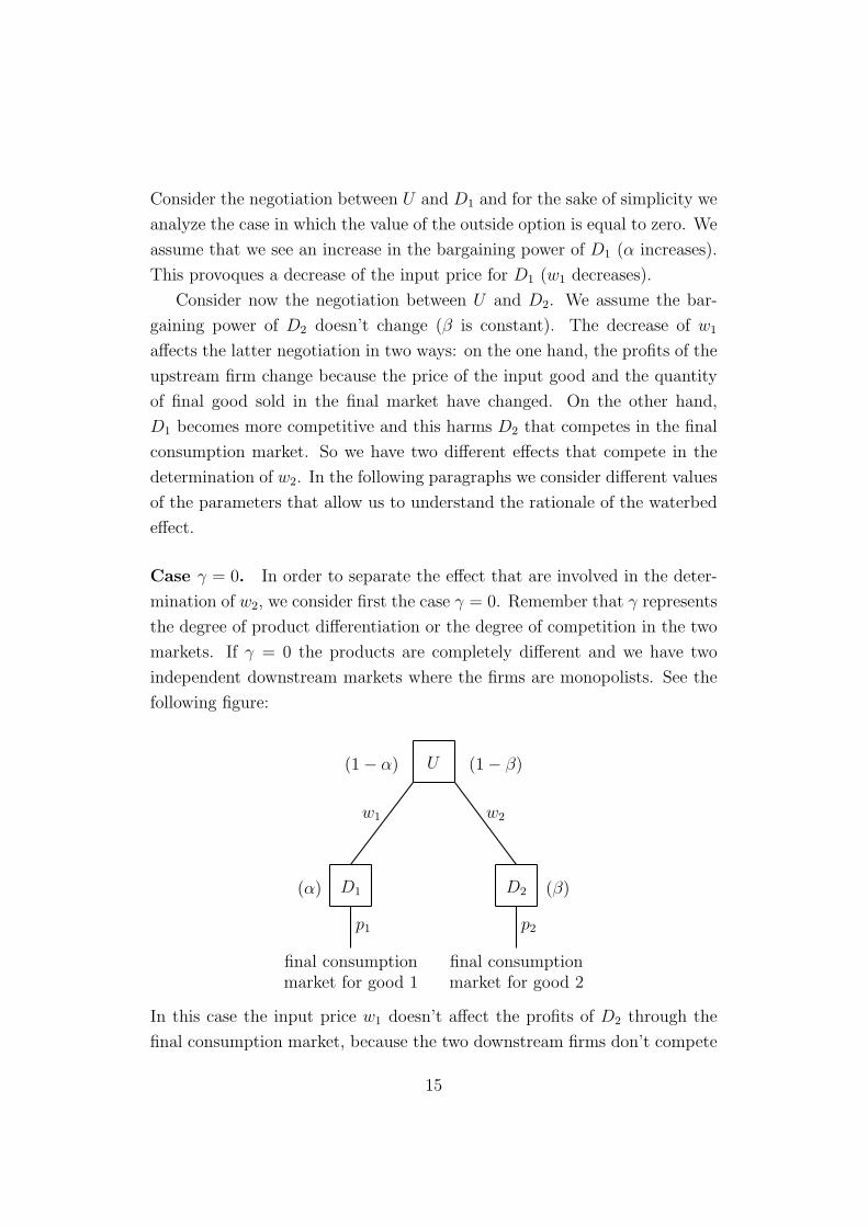
Case γ = 0. In order to separate the effect that are involved in the deter-

mination of w2, we consider first the case γ = 0. Remember that γ represents

the degree of product differentiation or the degree of competition in the two

markets. If γ = 0 the products are completely different and we have two

independent downstream markets where the firms are monopolists. See the

following figure:

U

D1 D2

w2w1

(β)(α)

(1− β)(1− α)

p1 p2

final consumptionmarket for good 1

final consumptionmarket for good 2

In this case the input price w1 doesn’t affect the profits of D2 through the

final consumption market, because the two downstream firms don’t compete

15

one against the other. Hence, we can analyze the effect through the upstream

market. Whether the profits of the upstream firm increase or not, it depends

on the elasticity of the demand function in the final consumption market. In

this case, it depends only on the elasticity of the demand function of market

where good 1 is sold.

On the one hand, when the demand is inelastic, a change in w1 doesn’t affect

the quantity sold q1 and then profits of U decrease. On the other hand,

when the demand is elastic, a decrease in w1 provoques a big increase of the

quantity sold, then the profits of U from selling to D1, w1q1(w1), increase.

With the specific linear demand function we used (pi = 1−qi−γqj), we have

that w1q1(w1) increases if and only if w1 > 12.

Consider now the case in which the demand in inelastic and then the

profits of U from selling to D1 decrease. Then, in the negotiation with

D2, the profits of the latter don’t depend on w1 and the profits of U have

decreased. Since the Nash bargaining solution maximizes the joint profits of

the parties, and the parties receive β% (D2) and (1− β)% (U) of the joints

profits, w2 has to compensate the losses of U , then w2 will increase and we

have the waterbed effect.

If the profits of U increase, then w2 will decrease.

Case γ ∈ [0, 1]. Fix a γ ∈ [0, 1]. When D1 becomes more efficient because

of an increment of α, then D2 have to compete in both downstream market

with a more efficient firm, and then its profits will decrease.

Consider now the negotiation between U and D2. The profits of both

parties are affected by the decrease of w1. The Nash bargaining solution will

compensate who results more harmed. If the losses of U are greater then the

ones of D2, then w2 will increase and we have the waterbed effect. In the

other case, in which the losses of D2 are greater, w2 decreases.

Hence, we can notice how the competition mitigates or even erases the

waterbed effect. Indeed, since the competition harms D2, its profits decrease

and then the Nash bargaining solution compensates it in order to recover the

losses due to the higher competition.

In particular, if we consider the negotiation between U and D2 we can

state the following proposition:

16

Proposition 4.3. In the negotiation between U and D2 solution price w2

increases when dw2

dw1

< 0.

When γ = 0, dw2

dw1

< 0 ←→ w1 ∈ (0, 1/2) and w2 ∈ (0, 1/2) ∀ β ∈ (0, 1).

When γ = 1, dw2

dw1

< 0 ←→ β ∈ (0, β) 5.

Proof. Consider the negotiation between U and D2. The first order condition

of this problem is:

Q = (1− β)πU

w2(w1, w2)

πU(w1, w2)+ β

πD2

w2(w1, w2)

πD2(w1, w2).

Using the implicit function theorem we have:

dw2

dw1

= −Qw1

Qw2

.

Using the specific demand function we introduced before, we have the fol-

lowing results:

γ = 0 if w1 ∈ (0, 1/2) and w2 ∈ (0, 1/2) for any β ∈ (0, 1) ←→ dw2

dw1

< 0

γ = 1 if β ∈ (0, β) ←→ dw2

dw1

< 0.

Notice that whether there is no downstream competition (γ = 0), the

profits of D2 doesn’t change and than the price w2 increases always when w1

and w2 are in the interval (0, 1/2).

When there is competition downstream, the waterbed effect arises only for

values of β < β.

4.5 Simulation

We simulated the results of our model introducing values of the parameters

in the first order conditions. Fixing β we can see how, due to an increase of

α, the input price w1 decreases and the input price w2 increases. In figure

1(a) we fixed γ = 0 and β = 0.2. Notice that the waterbed effect occurs for

α < 0.6; after this threeshold the input prices are negative. In figure 1(b) we

fixed γ = 1 and β = 0.6 and we find that the waterbed effect occurs only for

α ∈ (0.3, 0.8).

5β = f(w1, w2) where 0 < w2 < 1/2(√

2−1) and 0 < w1 < 1/2(4w2−1)+

√

1−6w2+6w2

2

2.

17

beta=0.2

0

0,05

0,1

0,15

0,2

0,25

0,3

0,35

0,4

0,45

0,1 0,2 0,3 0,4 0,5 0,6

alpha

w1

w2

(a)

beta=0.6

0

0,05

0,1

0,15

0,2

0,25

0,3

0,1 0,2 0,3 0,4 0,5 0,6 0,7

alpha

w1

w2

(b)

Figure 1: The input prices w1 and w2 for different values of α.

5 Welfare Analysis

In this section we analyze the effect of the waterbed effect on the consumers’

and total welfare.

5.1 Industry’s profits

Proposition 5.1. With completely differentiated products the total profits of

the industry increase if and only if −w′

1

w′

2

≥ w2

w1

.

With homogeneous products the total profits of the industry increases if and

only if 1−2w1−2w2 ≥ 0 and w′

1+w′

2 ≥ 0 or 1−2w1−2w2 ≤ 0 and w′

1+w′

2 ≤ 0.

Proof. The total profits of the industry are:

ΠI = ΠU + ΠD1+ ΠD2

Taking the derivatives we obtain:

∂ΠI

∂α=

[(

(γ − 2)γ + w1(6γ2 − 8)− 2γ3w2

)

∂w1

∂α+

(

(γ − 2)γ + w2(6γ2 − 8)− 2γ3w1

)

∂w2

∂α

]

(4− γ2)2.

The sign of ∂ΠI

∂αdepends on w1 and w2. We consider now the two extreme

cases, completely differentiated products (γ = 0) and homogeneous products

(γ = 1).

18

Differentiated products When γ = 0 we have:

∂ΠI

∂α= w1w

′

1 + w2w′

2.

The profits of the industry increase if and only if:

−w′

1

w′

2

≥ w2

w1

. (8)

Homogeneous products When γ = 1 we have:

∂ΠI

∂α= (1− 2w1 − 2w2)(w

′

1 + w′

2).

The profits of the industry increase if and only if:

1− 2w1 − 2w2 ≥ 0 or 1− 2w1 − 2w2 ≤ 0 (9)

w′

1 + w′

2 ≥ 0 w′

1 + w′

2 ≤ 0. (10)

With differentiated products, first of all, notice that if the waterbed

doesn’t occur, the profits of the industry always decrease: indeed, w′

2 is

positive, then (8) is never satisfied.

Since the two downstream firms are symmetric except the bargaining power,

we have that if α = β then w1 = w2 and that if α > β then w1 < w2. Hence,

consider two cases:

• i) When α < β, then w1 > w2. If −w′

1

w′

2

> 1, then the profits of the

industry is always increasing in α. This means that if D1 is the small

firm and its bargaining power increases, when there is waterbed effect

the profits of the industry increases.

• ii) When α > β, then w1 < w2. The sign of ∂ΠI

∂αdepends on the values

of the prices and their derivatives.

5.2 Consumers’ utility

Proposition 5.2. With completely differentiated products the consumers’

welfare increase if and only if −w′

1

w′

2

≥ 1+w2

1+w1

.

With homogeneous products the consumers’ welfare increases if and only if

w′

1 + w′

2 ≤ 0.

19

Proof. Following Singh and Vives [15], the demands we are using come from

the maximization problem of a representative consumer with utility separable

in money m given by:

U =q1 + q2 −q21

2− q2

2

2− γq1q2 + m

Substituting the optimal quantities and taking the derivatives we obtain:

∂U

∂α=

[(

(γ − 2)2 + w1(4− 3γ2)γ3w2

)

∂w1

∂α+

(

(γ − 2)2 + w2(4− 3γ2) + γ3w1

)

∂w2

∂α

]

(4− γ2)2.

As before, we consider the two extreme cases:

Differentiated products When γ = 0 we have:

∂U

∂α= −(1 + w1)w

′

1 − (1 + w1)w′

2.

The utility increases if and only if:

−w′

1

w′

2

≥ 1 + w2

1 + w1

. (11)

Notice again that when the waterbed effect doesn’t occur, equation (11) is

never satisfied.

Homogeneous products When γ = 1 we have:

∂U

∂α= −(1 + w1 + w2)(w

′

1 + w′

2).

The utility increases if and only if:

w′

1 + w′

2 ≤ 0. (12)

This means that, if the goods are perfectly homogeneous the utility of

the consumers increases if and only if the |w′

1| > |w′

2| (i.e. absolute value of

the discount obtained by D1 is greater than the increase of the price for D2).

20

5.3 Total welfare

Proposition 5.3. With completely differentiated products the total welfare

is always decreasing and with homogeneous products increases if and only if

(w′

1 + w′

2) < 0.

Proof. Consider now the total welfare:

∂TW

∂α=

∂ΠU

∂α+

∂U

∂α

When γ = 0, the total welfare never increases

w1w′

1 + w2w′

2 − (1 + w1)w′

1 − (1 + w1)w′

2 > 0

−2 > 0

When γ = 1, the total welfare increases if and only if (w′

1 + w′

2) < 0.

(1− 2w1 − 2w2)(w′

1 + w′

2)− (1 + w1 + w2)(w′

1 + w′

2) > 0

−3(w1 + w2)(w′

1 + w′

2) > 0

w′

1 + w′

2 < 0

With completely differentiated products the donwstream firms are monopo-

lists. Hence, an increase of α provoques a decrease of w1 and of p1.

6 Conclusions

If this paper we propose a rationale for the existence of the waterbed ef-

fect. We propose a complete model that captures the main features of the

strategic interactions among the upstream firm and the downstream firms

and that extends some limitations of other models proposing a theory for

such effect. Indeed in our paper we assume that the input prices are deter-

minated by bilateral negotiations between upstream and downstream firms

and we consider any distribution of bargaining power between the parties.

The rationale we propose differs from the ones proposed in the papers

closely related to mine (Valletti and Inderst [8] and Majumdar [11]). Here

the upstream firm is harmed by the strong donwstream firm because of the

21

discount that the latter obtains. For that reason, the upstream firm wants to

recover the losses in the negotiation with the other downstream firm. When

the other downstream firm is not harmed through the final consumption

market, then the price increases and the waterbed effect occurs. Instead,

when the downstream competition is intense enough, the gains in efficiency

obtained by the strong downstream firm harm the other downstream firm

and it will be the latter that will recover the losses obtaining a discount in

the negotiation. In this case the price for the weak firm decreases.

Hence, we can notice how in this model the competition mitigates or even

eliminates the waterbed effect.

The added value of this paper is that it generalizes the distribution of

bargaining power between the parties involved in the negotiations. Valletti

and Inderst in [8] assume that the upstream firm is a monopolist that makes

a take-it-or-leave-it offer. Here we relax this assumption allowing for any

distribution of power between upstream and downstream firms and we obtain

a more complete framework. What we find at the end is that the total

welfare always increases with completely differentiated goods and increases

when w′

1 + w′

2 < 0 with homogeneous goods.

The explication is the following: consider the case of completely differ-

entiated products. On the one hand, when the bargaining power of one

downstream firm is low, the upstream firm behaves as a monopolist in the

intermediate market and the downstream firm as a monopolist in the final

consumption market. Then we have a double marginalization problem. On

the other hand, when the downstream firm is relatively strong in the nego-

tiation, the margin of the upstream firm falls, the double marginalization

problem falls as well, then the final price for the consumers decreases and

then the total profits increase.

A Cost asymmetries

In this appendix we study the effect of a variation in the marginal production

cost of one downstream firm on the wholesale prices. In this preliminary

version we don’t have any results. What it follows is the setting we are

considering.

22

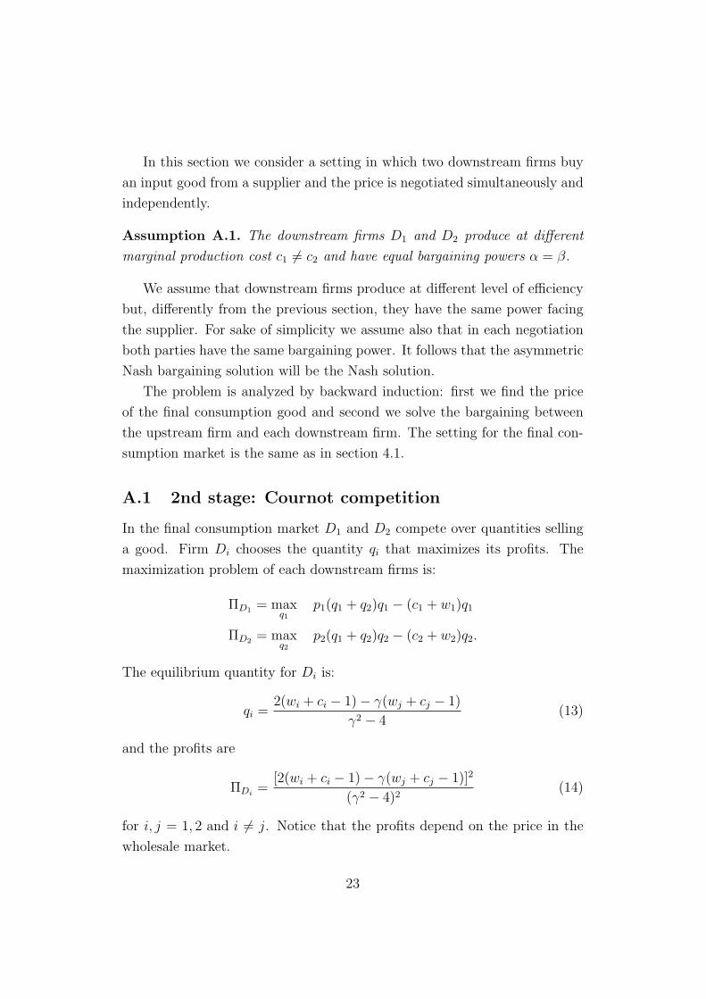
In this section we consider a setting in which two downstream firms buy

an input good from a supplier and the price is negotiated simultaneously and

independently.

Assumption A.1. The downstream firms D1 and D2 produce at different

marginal production cost c1 6= c2 and have equal bargaining powers α = β.

We assume that downstream firms produce at different level of efficiency

but, differently from the previous section, they have the same power facing

the supplier. For sake of simplicity we assume also that in each negotiation

both parties have the same bargaining power. It follows that the asymmetric

Nash bargaining solution will be the Nash solution.

The problem is analyzed by backward induction: first we find the price

of the final consumption good and second we solve the bargaining between

the upstream firm and each downstream firm. The setting for the final con-

sumption market is the same as in section 4.1.

A.1 2nd stage: Cournot competition

In the final consumption market D1 and D2 compete over quantities selling

a good. Firm Di chooses the quantity qi that maximizes its profits. The

maximization problem of each downstream firms is:

ΠD1= max

q1

p1(q1 + q2)q1 − (c1 + w1)q1

ΠD2= max

q2

p2(q1 + q2)q2 − (c2 + w2)q2.

The equilibrium quantity for Di is:

qi =2(wi + ci − 1)− γ(wj + cj − 1)

γ2 − 4(13)

and the profits are

ΠDi=

[2(wi + ci − 1)− γ(wj + cj − 1)]2

(γ2 − 4)2(14)

for i, j = 1, 2 and i 6= j. Notice that the profits depend on the price in the

wholesale market.

23

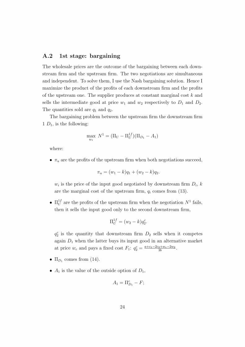
A.2 1st stage: bargaining

The wholesale prices are the outcome of the bargaining between each down-

stream firm and the upstream firm. The two negotiations are simultaneous

and independent. To solve them, I use the Nash bargaining solution. Hence I

maximize the product of the profits of each downstream firm and the profits

of the upstream one. The supplier produces at constant marginal cost k and

sells the intermediate good at price w1 and w2 respectively to D1 and D2.

The quantities sold are q1 and q2.

The bargaining problem between the upstream firm the downstream firm

1 D1, is the following:

maxw1

N1 = (ΠU − Π1fU )(ΠD1

− A1)

where:

• πu are the profits of the upstream firm when both negotiations succeed,

πu = (w1 − k)q1 + (w2 − k)q2.

wi is the price of the input good negotiated by downstream firm Di, k

are the marginal cost of the upstream firm, qi comes from (13).

• Π1fU are the profits of the upstream firm when the negotiation N1 fails,

then it sells the input good only to the second downstream firm,

Π1fU = (w2 − k)qc

2.

qc2 is the quantity that downstream firm D2 sells when it competes

again D1 when the latter buys its input good in an alternative market

at price wc and pays a fixed cost F1: qc2 = a+c1−2c2+wc−2w2

3b.

• ΠD1comes from (14).

• A1 is the value of the outside option of D1,

A1 = ΠcD1− F ;

24

where ΠcD1

are the profits of D1 when the bargaining process fails and

it has to pay the input good wc:

πcD1

=[2(wc + ci − 1)− γ(wj + cj − 1)]2

(γ2 − 4)2.

Furthermore, F are fixed cost that D1 must pay in order to enter in

the alternative market.

The negotiation between U and D2 is the following:

maxw2

N2 = (ΠU − Π2fU )(ΠD2

− A2).

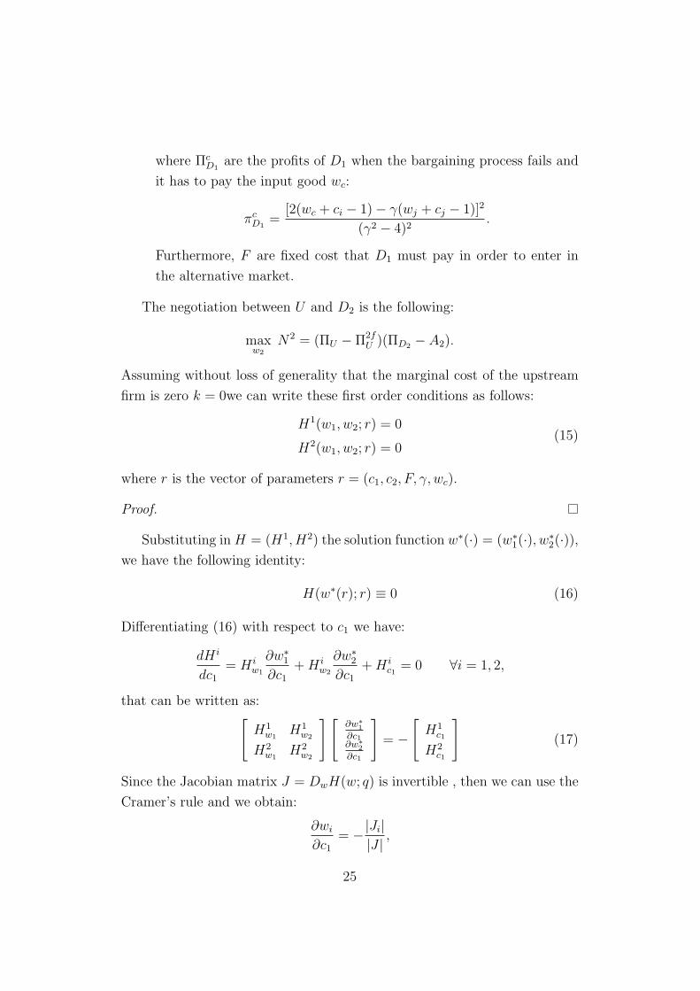
Assuming without loss of generality that the marginal cost of the upstream

firm is zero k = 0we can write these first order conditions as follows:

H1(w1, w2; r) = 0

H2(w1, w2; r) = 0(15)

where r is the vector of parameters r = (c1, c2, F, γ, wc).

Proof.

Substituting in H = (H1, H2) the solution function w∗(·) = (w∗

1(·), w∗

2(·)),we have the following identity:

H(w∗(r); r) ≡ 0 (16)

Differentiating (16) with respect to c1 we have:

dH i

dc1

= H iw1

∂w∗

1

∂c1

+ H iw2

∂w∗

2

∂c1

+ H ic1

= 0 ∀i = 1, 2,

that can be written as:[

H1w1

H1w2

H2w1

H2w2

][

∂w∗

1

∂c1∂w∗

2

∂c1

]

= −[

H1c1

H2c1

]

(17)

Since the Jacobian matrix J = DwH(w; q) is invertible , then we can use the

Cramer’s rule and we obtain:

∂wi

∂c1

= −|Ji||J | ,

25

where |Ji| is the matrix obtained by replacing the ith column of the Jacobian

J with the vector (H1c1

, H2c1

)T .

We can write the derivatives as follows:

∂w∗

1

∂c1

= − H1c1

H2w2−H2

c1H1

w2

H1w1

H2w2−H2

w1H1

w2

=H2

c1H1

w2−H1

c1H2

w2

D(18)

∂w∗

2

∂c1

= − H1w1

H2c1−H2

w1H1

c1

H1w1

H2w2−H2

w1H1

w2

=H2

w1H1

c1−H1

w1H2

c1

D, (19)

where

D ≡ H1w1

H2w2−H2

w1H1

w2.

References

[1] Chae S. and Heidhues P. (1999), “The Effects of Downstream Distributor

Chains on Upstream Producers Entry: A Bargaining Perspective”, CIC

Working Papers, Berlin.

[2] Chae S. and Heidhues P. (2004), “Buyers’ Alliances for Bargaining

Power”, Journal of Economics & Management Strategy, 13, 731-754.

[3] Faulı-Oller R. and Sandonıs J. (2003), “To merge or to license: im-

plications for competition policy”, International Journal of Industrial

Organization, 21, 655-672.

[4] Genakos C and Valletti T. (2007), “Testing the “waterbed” effect in the

mobile telephony”, Working Paper, May.

[5] Katz M. L. (1987), “The welfare effects of third degree price discrimi-

nation”, American Economic Review, 77, 154-167.

[6] Inderst R. (2007), “Leveraging buyer power”, International Journal of

Industrial Organization, 25, 908-924.

[7] Inderst R. and Mazzarotto N. (2006), “Buyer power. Sources, Conse-

quences, and Policy Responses”.

26

[8] Inderst R. and Valletti T. (2007), “Buyer power and the waterbed ef-

fect”, Working Paper.

[9] Inderst R. and Wey C. (2003), “Bargaining, Mergers, and Technology

Choice in Bilaterally Oligopolistic Industries”, The RAND Journal of

Economics, 34, 1-19.

[10] Motta M. (2004), Competition Policy. Theory and practice, Cambridge

University Press, Cambridge.

[11] Majumdar A. (2007), “Waterbed Effect And Buyer Merger”, Centre for

Competition Policy, University of East Anglia, CCP Working Paper,

May. International Journal of Industrial Organization, 24, 715-731.

[12] Shapiro C. and Kaplow L. (2007), “Antitrust”, in Handbook of Law and

Economics, forthcoming.

[13] Salop C. (1979), “Monopolistic Competition with Outside Goods”, The

Bell Journal of Economics, 10, 141-156.

[14] Sandonıs J. and Faulı-Oller R. (2006), “On the competitive effects of

vertical integration by a research laboratory”, International Journal of

Industrial Organization, 24, 715-731.

[15] Singh N. and Vives X. (1984), “Price and Quantity Competition in a

Differentiated Duopoly”, RAND Journal of Economics, 15, 546-554.

[16] Raskovich A. (2007), “Ordered bargaining”, Industrial Journal of In-

dustrial Organization, 25, 1126-1143.

[17] Tirole J. (2003), The theory of industrial organization, The MIT Press,

Cambridge, Massachusetts.

[18] UK Competition Commision (2007), Grocery Market Investigation,

available at this webpage www.competition-commission.org.uk/

inquiries/ref2006/grocery/pdf/emerging_thinking.pdf.

[19] UK Competition Commision (2007), Market investigation into

the supply of groceries in the UK, available at this webpage

27

http://www.competition-commission.org.uk/rep_pub/reports/

2008/538grocery.htm.

28