Embed Size (px)
Citation preview
HAL Id: tel-00011404https://tel.archives-ouvertes.fr/tel-00011404
Submitted on 18 Jan 2006
HAL is a multi-disciplinary open accessarchive for the deposit and dissemination of sci-entific research documents, whether they are pub-lished or not. The documents may come fromteaching and research institutions in France orabroad, or from public or private research centers.
L’archive ouverte pluridisciplinaire HAL, estdestinée au dépôt et à la diffusion de documentsscientifiques de niveau recherche, publiés ou non,émanant des établissements d’enseignement et derecherche français ou étrangers, des laboratoirespublics ou privés.
Dosimétrie personnalisée par simulation Monte CarloGATE sur grille de calcul. Application à la curiethérapie
oculaire.Lydia Maigne
To cite this version:Lydia Maigne. Dosimétrie personnalisée par simulation Monte Carlo GATE sur grille de calcul. Ap-plication à la curiethérapie oculaire.. Physique des Hautes Energies - Expérience [hep-ex]. UniversitéBlaise Pascal - Clermont-Ferrand II, 2005. Français. <tel-00011404>
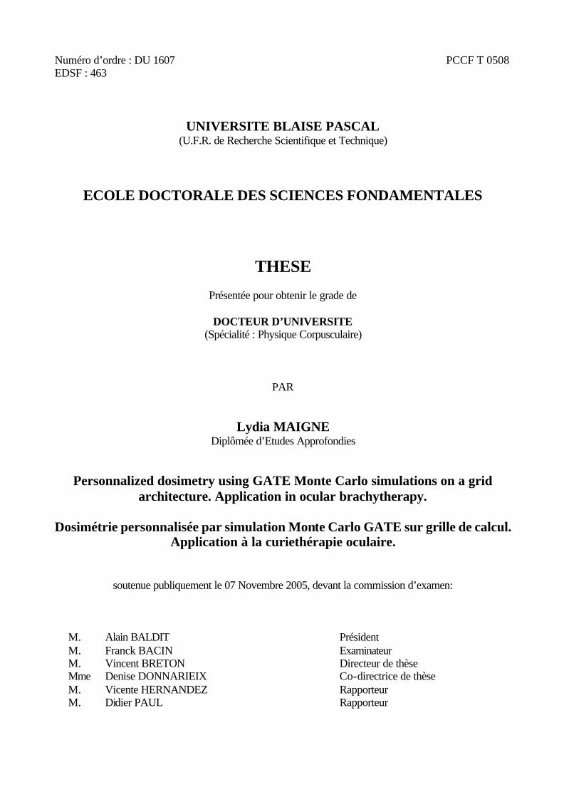
Numéro d’ordre : DU 1607 PCCF T 0508 EDSF : 463
UNIVERSITE BLAISE PASCAL (U.F.R. de Recherche Scientifique et Technique)
ECOLE DOCTORALE DES SCIENCES FONDAMENTALES
THESE
Présentée pour obtenir le grade de
DOCTEUR D’UNIVERSITE (Spécialité : Physique Corpusculaire)
PAR
Lydia MAIGNE Diplômée d’Etudes Approfondies
Personnalized dosimetry using GATE Monte Carlo simulations on a grid architecture. Application in ocular brachytherapy.
Dosimétrie personnalisée par simulation Monte Carlo GATE sur grille de calcul.
Application à la curiethérapie oculaire.
soutenue publiquement le 07 Novembre 2005, devant la commission d’examen:
M. M. M. Mme M. M.
Alain BALDIT Franck BACIN Vincent BRETON Denise DONNARIEIX Vicente HERNANDEZ Didier PAUL
Président Examinateur Directeur de thèse Co-directrice de thèse Rapporteur Rapporteur


A mes parents, A mes grand-parents,
A ma famille et mes amis.

Remerciements Le travail d’un doctorant est fondé en grande partie sur le support de son Laboratoire, de son équipe de recherche ainsi que de toutes les personnes rencontrées au cours des projets dans lesquels il est impliqué. Pour ma part, c’est bien grâce à toutes ces nombreuses collaborations effectuées au cours de ma thèse que mon étude a pu s’exprimer dans son intégralité. Le Laboratoire de Physique Corpusculaire a hébergé mes premiers pas dans le monde de la recherche ; d’abord au cours d’un stage JANUS au sein de l’équipe thermoluminescence puis au cours de mon stage de maîtrise dans l’équipe PCSV qui m’accueillera dans la suite de mon parcours de jeune chercheur lors d’un stage de DEA puis de ma thèse. Je tiens donc à remercier toutes les personnes m’ayant donné le goût pour la recherche mais aussi pour la persévérance ! Tout d’abord je tiens particulièrement à remercier Vincent Breton qui m’a fait confiance pour mener à bien la mission qui m’était confiée : participer au développement de la plate-forme de simulation GATE pour la dosimétrie mais aussi exploiter et appréhender les possibilités informatiques offertes par les grilles de calcul. Le challenge était de taille mais je voudrais te remercier Vincent, de m’avoir toujours lancé des défis, c’est bien grâce à ton exigence que j’ai pu évoluer tel que je l’ai fait au cours de ces trois années. Grâce à la co-direction de ma thèse par Denise Donnarieix, j’ai pu faire avancer mon travail en gardant toujours à l’idée cette finalité : tout travail de recherche en physique médicale doit toujours s’accompagner d’une concrétisation ou d’un bénéfice dans le traitement des tumeurs pour le patient. Merci pour ta présence et ton soutien tout au long de cette thèse. Tu as pu m’aider à garder un pied dans le monde la physique médicale et m’a toujours accueillie avec disponibilité au Centre Jean Perrin lorsque mes recherches l’exigeaient. Didier Paul, professeur à l’Université de Marseille II, spécialiste de la radioprotection, issu lui même d’une formation en physique médicale, m’a fait le grand plaisir de juger et commenter ce travail de thèse. Je tiens également à exprimer toute ma reconnaissance à Vicente Hernandez, professeur d’informatique à l’Université polytechnique de Valence en Espagne, pour avoir accepté d’être rapporteur. Je le remercie encore de m’avoir si bien accueillie à Valence pour présenter notre travail devant des médecins et physiciens médicaux espagnols.
Je désire adresser un remerciement tout particulier au professeur en ophtalmologie au Centre Hospitalier Gabriel Montpied de Clermont-Ferrand, Mr Franck Bacin, pour avoir accepté de faire partie de mon jury de thèse. L’excellence de votre travail ainsi que votre simplicité sont pour moi essentiels au jugement et à la critique de ma thèse. Merci également à Alain Baldit, directeur du Laboratoire de Physique Corpusculaire, pour la présidence de mon jury. Mon intégration dans la collaboration GATE depuis 2002 m’a permis de rencontrer et d’interagir avec de nombreux scientifiques travaillant dans le domaine de l’imagerie nucléaire ainsi que de la dosimétrie. Je voudrais remercier toutes les personnes ayant participé à mon épanouissement scientifique et m’ayant encouragée et guidée dans mes travaux de recherche : Christian Morel, Irène Buvat, Dennis Schaart, Assen Kirov, Manuel Bardiès, Sophie Kerhoas et tous les autres. Merci aussi à Sébastien Incerti et Michel Maire, faisant partie de la collaboration GEANT4, pour leur aide précieuse au cours de ces trois années. Les projets européens DataGrid et EGEE, dirigés tous deux jusqu’à cette année par Fabrizio Gagliardi, m’ont fait évoluer au sein de la recherche informatique et physique européenne. Je tiens particulièrement à remercier Fabrizio pour l’attention et la confiance qu’il m’a accordées dans ma prise de responsabilités au sein de cette collaboration pour les applications GATE. Merci aussi à Johan Montagnat pour son aide et son soutien en tant que responsable des applications biomédicales dans le projet EGEE. Je tiens aussi à ne pas oublier toutes les personnes avec lesquelles j’ai travaillé pour valoriser nos applications biomédicales auprès de la commission européenne : Roberto Barbera, Alberto Falzone, Ignacio Blanquer, Geneviève Romier, René Metery, Adeline Eynard, et tout particulièrement Yannick Legré avec lequel j’ai réalisé la démonstration de la « gridification » de GATE au cours de la clôture du projet DataGrid. Merci à toute l’équipe PCSV, aux thésards, aux ingénieurs pour m’avoir toujours aidée quand j’en avais besoin. Ziad, Cheick et Nicolas ; Florence, Jean, Emmanuel, Yannick encore et toujours, j’espère ne pas vous avoir trop ennuyés et stressés par mes questions et mes requêtes, merci pour votre soutien sans failles! Merci aussi aux stagiaires accueillis dans l’équipe pour leur aide au cours de cette thèse : Lucie, Romain, Joël, Jérôme et Florence. Merci également à David Hill pour sa disponibilité et son aide concernant l’utilisation de nombres pseudo-aléatoires dans nos simulations. Ces trois années n’ont pas du être les plus faciles à vivre pour mes amis et ma famille, je peux avouer, maintenant que tout se termine, que je leur en ai fait voir de toutes les couleurs ! Alors, d’abord toutes mes excuses si je n’ai pas toujours été disponible quand il le fallait, et permettez-moi de vous dire un grand merci pour tout l’amour que vous m’avez apporté durant mon parcours. Merci à mes grand-parents pour m’avoir épaulée (merci à ma grand-mère pour ses bons petits repas et son aide précieuse !), merci à mes parents, toujours présents (une pensée pour mon chat, qui a été mon régulateur de stress !), merci à Carole pour sa disponibilité et tous les moments de détente que nous avons pu passer ensemble, merci à tous les autres… et surtout merci à Jean Noël.
Contents INTRODUCTION GENERALE 1 GENERAL INTRODUCTION 7 CHAPTER I. 11 OCULAR BRACHYTHERAPY USING 106RU/106RH OPHTHALMIC APPLICATORS 11 INTRODUCTION 11 I.1. OCULAR BRACHYTHERAPY: A CLINICAL APPROACH 12 I.1.1. Ocular melanoma and benign tumour 12 I.1.1.A. Eye anatomy and tumour incidence 12 I.1.1.A.1. Eye tissues 12 I.1.1.A.2. Different type of tumours treated with 106Ru plaques 13 I.1.1.B. Tumour diagnosis 13 I.1.1.B.1. Photography 14 I.1.1.B.2. Ultrasound (echography) 14 I.1.1.B.3. Magnetic Resonnance Imaging (MRI) 14 I.1.1.B.4. Other diagnosis modalities: Biopsy and metastases detection 15 I.1.2. 106Ru/106Rh definition 15 I.1.3. The ophthalmic applicators 17 I.1.4. Dose prescription and treatment efficacy 18 I.1.4.A. The Collaborative Ocular Melanoma Study (COMS) 18 I.1.4.B. Treatments using 106Ru/106Rh ophthalmic applicators 19 I.1.4.C. Other radiotherapy and brachytherapy treatments 20 I.1.4.C.1. Ocular brachytherapy using 125I ophthalmic plaques 20 I.1.4.C.2. Ocular brachytherapy using bi-nuclide radioactive ophthalmic applicators 21 I.1.4.C.3. The protontherapy 22 I.2. QUALITY CONTROL AND DOSE MEASUREMENTS 23 I.2.1. Measurements 23 I.2.1.A. Absolute calibration of beta sources: the extrapolation chamber 23 I.2.1.B. Radiochromic film (RCF) 24 I.2.1.B.1. Radiochromic film calibrations 24 I.2.1.C. Thermoluminescence dosimeters (TLD) 25 I.2.1.D. Alanine pellets 25 I.2.1.E. Scintillator 25 I.2.1.F. Diamond 26 I.2.1.G. Diode 26 I.2.1.H. Polymer gel 26 I.2.1.I. Well type ionization chamber 26 I.2.2. Utilization of detectors in clinical routine 27 I.2.2.A. Detectors not well adapted 27

I.2.2.A.1. Extrapolation chamber 27 I.2.2.A.2. Polymer gel 27 I.2.2.A.3. TLD 27 I.2.2.A.4. Diamond detector 27 I.2.2.A.5. Alanine 28 I.2.2.B. Well adapted detectors 28 I.2.2.B.1. Well-type ionization chamber 28 I.2.2.B.2. Plastic scintillator 28 I.2.2.B.3. Plane-parallel ionization chamber 28 I.2.2.B.4. Diode 28 I.2.2.B.5. Radiochromic film 28 I.2.3. Phantom characterizations 28 I.3. QUALITY CONTROL OF OPHTHALMIC APPLICATORS 30 I.3.1. Parameters to study 30 I.3.1.A. Average radius (R50) 30 I.3.1.B. Source strength 30 I.3.1.B.1. Source strength specification by manufacturer 30 I.3.1.C. Source non-uniformity 31 I.3.1.D. Source asymmetry 32 I.3.2. Ophthalmic applicators calibration performed by BEBIG 32 I.3.2.A. Dose prescription modifications with NIST and ASMW calibrations 32 I.4. TREATMENT PLANNING USING PLAQUE SIMULATOR 33 I.4.1. Positioning the plaque on the eye 34 I.4.2. Calculating and displaying the dose distribution 34 I.4.2.A. The patch source dose function 34 I.4.2.A.1. The source strength S 35 I.4.2.A.2. The calibration constant A 35 I.4.2.A.3. The geometry factor G(r) 35 I.4.2.A.4. The radial dose function g(r) 36 I.4.2.A.5. The anisotropy function F(r,j) 37 I.4.2.B. Dosimetric calculations with Plaque Simulator in practice 37 CONCLUSION 39 References 39 CHAPTER II. 43 GRID TECHNOLOGIES AND HEALTH RELATED APPLICATIONS 43 INTRODUCTION 43 II.1. GRID FOR HEALTH RELATED APPLICATIONS 44 II.1.1. The challenges for eHealth 44 II.1.2. The HealthGrid association 45 II.1.3. Health grids: a grid scenario for radiotherapy planning (from the HealthGrid white paper [50 ]) 46 II.1.3.A. Processing simulations in a grid environment 46 II.1.3.B. Issues for therapy planning 46 II.1.3.B.1. A grid scenario for radiotherapy planning and treatment 47 II.2. GRID COMPUTING IN EUROPE 48 II.2.1. European and national grid projects 49 II.2.2. The European Datagrid Project (EDG) 50 II.2.2.A. Organization 50 II.2.2.B. Achievements and lessons learned 52 II.3. THE EGEE (ENABLING GRID FOR E-SCIENCE) PROJECT 53 II.3.1. Presentation 53 II.3.1.A.1. EGEE activities 53

II.3.1.A.2. The objectives of the NA4 54 II.3.1.B. The EGEE infrastructure 55 II.3.1.B.1. The Grid middleware 55 II.3.1.B.2. Machines and services part of the EGEE infrastructure 57 II.3.1.B.3. A typical job flow in EGEE 60 II.3.1.C. Requirements for a user to access the grid 62 II.3.1.C.1. Obtaining a certificate 62 II.3.1.C.2. Be part of a Virtual Organization (VO) 62 II.3.2. The grid computing efficacy 65 II.3.2.A. Workload data analysis on computing resources 65 II.3.2.B. Job requirements 67 II.3.2.C. Managing medical data in a grid environment 69 II.3.2.C.1. Storage and retrieval 69 II.3.2.C.2. Security and privacy 71 CONCLUSION 72 References 72 CHAPTER III. 75 THE GATE MONTE CARLO SIMULATION PLATFORM FOR DOSIMETRIC APPLICATIONS 75 INTRODUCTION 75 III.1. GATE: A MONTE CARLO PLATFORM FOR DOSIMETRY 76 III.1.1. Functionalities available and requirements for dosimetry applications 76 III.1.1.A. Geometry and Systems 76 III.1.1.A.1. Existing functionalities 76 III.1.1.A.2. Needed functionalities 76 III.1.1.B. Voxelized sources and phantoms: GATE calculations based on CT data 77 III.1.1.B.1. Definition of DICOM and Interfile formats 77 III.1.1.B.2. Needed functionalities 85 III.1.1.C. Source and detector movements, source decay 86 III.1.1.C.1. Existing functionalities 86 III.1.1.D. Information on interactions in media and output data 87 III.1.1.D.1. Existing functionalities 87 III.1.1.D.2. Needed functionalities 87 III.1.2. Platform improvements for dosimetric applications 88 III.1.2.A. Variance reduction techniques implementation in GATE 88 III.1.2.A.1. The geometrical importance sampling 88 III.1.2.A.2. Pulse height tallies 89 III.1.2.B. Visualisation of medical images in 3 dimensions 91 III.1.2.C. The parameterised volumes in GATE simulations 94 III.1.2.C.1. Particle transport in Geant4 94 III.1.2.C.2. Parameterised volume 94 III.2. VALIDATION OF GEANT4 ELECTROMAGNETIC PHYSICS FOR ELECTRONS 95 III.2.1. Interactions of electrons 95 III.2.1.A. Inelastic interaction with atomic electrons: ionization process 95 III.2.1.B. Inelastic interaction of electrons with nuclei: Bremsstrahlung 96 III.2.1.C. Electron stopping powers and ranges 96 III.2.2. Geant4 electromagnetic physics packages 97 III.2.2.A. The Standard package 98 III.2.2.A.1. The ionization process in the standard package 98 III.2.2.A.2. The bremsstrahlung process in the standard package 98 III.2.2.B. The Low Energy package: evaluated data driven approach 98 III.2.2.B.1. The ionization process in the Low Energy package 99
III.2.2.B.2. The Bremsstrahlung process in the Low Energy package 100 III.2.2.C. The Low Energy package: analytic approach 100 III.2.2.D. Specification of the GEANT4 physic processes in GATE 101 III.2.3. Multiple scattering implementation in GEANT4 101 III.2.3.A. The angular distribution 102 III.2.3.A.1. The tail of the distribution 102 III.2.3.A.2. The width of the angular distribution: correction of the Highland formula 103 III.2.3.B. The path length correction PLC 103 III.2.4. The step control and boundary crossing parameters in GEANT4 104 III.2.5. Evaluations and comparisons of stopping power and CSDA range for electrons 105 III.2.6. Beta ray point source dose distributions 106 III.2.6.A. Introduction 106 III.2.6.B. Monte Carlo calculation details 106 III.2.6.B.1. Uncertainties evaluation 107 III.2.6.C. Results 107 III.2.6.C.1. Monoenergetic beta point source dose kernels 107 III.2.6.C.2. Beta dose point kernels for 106Rh polyenergetic source 119 CONCLUSION 122 References 123 CHAPTER IV. 125 106RU/106RH OCULAR BRACHYTHERAPY TREATMENT PLANNING USING GATE. PRELIMINARY STUDIES USING CT IMAGES. 125 INTRODUCTION 125 IV.1. 106RU/106RH OCULAR BRACHYTHERAPY TREATMENT PLANNING USING GATE 126 IV.1.1. Theoretical calculation of the beta point source dose function for 106Ru/106Rh eye applicators, comparisons 126 IV.1.1.A. The function of Loevinger 126 IV.1.1.A.1. Definition 126 IV.1.2. Monte Carlo calculations of ocular brachytherapy treatments using 106Ru/106Rh ophthalmic applicators, comparisons 128 IV.1.2.A. GATE Monte Carlo calculation details 128 IV.1.2.A.1. Description 128 IV.1.2.A.2. Uncertainties evaluation 129 IV.1.2.B. Dose distribution on the central axis 129 IV.1.2.B.1. Influence of the cut value on electrons 129 IV.1.2.B.2. Evaluation of the impact of gamma rays on the dose deposited 131 IV.1.2.B.3. Comparisons and results 131 IV.1.2.C. Isodoses on the median plan 136 IV.1.2.D. Conclusion 145 IV.2. DOSIMETRIC STUDY FOR ELECTRONS IN TISSUE 146 IV.2.1. Correlation between CT numbers and tissue parameters needed for GATE simulations of clinical dose distributions 146 IV.2.1.A. Introduction 146 IV.2.1.B. X-ray attenuation coefficient and CT numbers 147 IV.2.1.C. Calculation of the CT numbers of human tissues 147 IV.2.1.C.1. Determination of the parameters k1 and k2 148 IV.2.1.C.2. Usage of interpolation functions to fit Hounsfield units to tissue parameters 152 IV.2.1.D. Conversion of Hounsfield units into tissue parameters for GATE simulations 157 IV.2.1.E. Influence of the media compositions on dosimetry 160 IV.2.1.F. Conclusion 165 CONCLUSION 165

References 166 CHAPTER V. 167 GATE APPLICATIONS IN A GRID ENVIRONMENT 167 INTRODUCTION 167 V.1. PARALLELIZATION OF GATE SIMULATIONS WITHIN EGEE 167 V.1.1. The installation 167 V.1.2. The parallelisation of GATE simulations and tests of submission to a grid environment 169 V.1.2.A. Introduction 169 V.1.2.B. The Random Number Generator (RNG) in Monte Carlo simulations 170 V.1.2.B.1. Principle 170 V.1.2.B.2. The parallelization of RNGs 171 V.1.2.C. Application of the parallel method 173 V.1.2.D. Sending the simulations on a grid environment 175 V.1.2.D.1. The Java Job Submission (JJS) tool 175 V.1.2.D.2. First approach for a web portal prototype to submit GATE simulations on the EDG testbed 176 V.1.2.E. Results 177 V.1.2.F. Comparison of the physical results 178 V.1.2.G. Tests of computing time using the JJS tool. 179 V.1.2.G.1. Influence of the number of threads on the computing time 179 V.1.2.G.2. Influence of partitioning on computing time. 180 V.1.2.H. Tests of computing time on the EGEE testbed using the usual LCG-2 jobs submission [22 ] 183 V.1.2.H.1. Influence of the jobs various status times 183 V.1.2.H.2. Influence of the jobs global computing times 184 V.1.2.I. Conclusion and future prospects 185 V.2. GATE APPLICATIONS ON THE GENIUS WEB PORTAL 186 V.2.1. Architecture and implementation of the portal 186 V.2.2. Encoded functionalites for GATE applications on the Genius web portal 187 V.2.2.A. Test phase on the GILDA infrastructure 188 V.2.2.B. Implementation of GATE functionalities 188 V.2.2.B.1. The files configuration 188 V.2.2.B.2. Creation of the GATE files 190 V.2.2.B.3. Creation of the JDL files 192 V.2.2.B.4. Launching of the simulations on the EGEE infrastructure 195 V.2.2.B.5. Job Monitoring and retrieving 197 V.2.2.B.6. Some remarks 199 V.3. DEISA AND EGEE: GATE PILOT APPLICATION ON A JOINT INFRASTRUCTURE 199 CONCLUSION 201 References 201 GENERAL CONCLUSION 203 CONCLUSION GENERALE 207 FIGURES AND TABLES 211 FIGURES 211 TABLES 217 PUBLICATIONS AND OTHER WORK 219

Introduction générale
1
Introduction générale La méthode Monte Carlo est un algorithme de calcul permettant de modéliser au plus près la physique liée aux processus de dépôts d’énergie, les algorithmes Monte Carlo sont donc prévus pour être plus précis que d’autres types d’algorithmes de calcul. Cependant, des calculs précis utilisant Monte Carlo conduisent à des temps de calcul très importants en comparaison avec les logiciels analytiques utilisés en routine clinique pour la planification des traitements du cancer. Pour résoudre ce problème, différents codes Monte Carlo ont déjà été développés pour un usage dédié à la radiothérapie. Les approximations ou les compromis mis en jeu dans ces codes, comme une modification du transport des électrons, une limitation du suivi des événements les moins probables, une méthode de transport des particules basée sur le passage de voxels, etc, permettent effectivement une réduction des temps de calcul. Dans l’équipe PCSV (Plate-forme de Calcul pour les Sciences du Vivant), membre du Laboratoire de Physique Corpusculaire de Clermont-Ferrand, la plate-forme de simulation Monte Carlo GATE (GEANT4 Application for Tomographic Emission) est utilisée dans les domaines d’applications liés à l’imagerie SPECT, TEP, à la radiothérapie et à la curiethérapie. De manière à étendre les qualités intrinsèques de GATE aux applications en dosimétrie, et après la release publique de GATE en mai 2004, la collaboration OpenGATE a mis en place deux groupes de travail pour étudier plus spécifiquement les aptitudes de la plate-forme de simulation pour la dosimétrie, un deuxième groupe est consacré à la réduction des temps de calcul des simulations en les divisant entre autre sur de multiples processeurs. Ces nouveaux champs de travail permettront à la plate-forme de rivaliser avec les codes de calcul Monte Carlo existant pour une utilisation en dosimétrie personnalisée exploitant des images voxélisées pour modéliser l’anatomie du patient. L’objectif de cette thèse était de valider la plate-forme GATE pour des calculs en dosimétrie utilisant des électrons et de déployer cette plate-forme sur un environnement de grille de calcul afin de réduire son temps d’exécution. Un prototype permettant la division, la répartition et le lancement des simulations GATE sur une architecture de grille est proposé pour permettre aux praticiens et physiciens médicaux de délivrer des distributions de dose de manière rapide et précise en utilisant un algorithme Monte Carlo. La curiethérapie oculaire utilisant des applicateurs ophtalmiques émetteurs bétas est l’application qui a bénéficié de nos recherches concernant les électrons et les calculs sur grille.
Introduction générale
2
Les traitements utilisant des faisceaux d’électrons ainsi que la curiethérapie utilisant ces mêmes rayonnements représentent 10 à 15 % des traitements quotidiens en routine clinique. Au Centre Jean Perrin de Clermont-Ferrand, les traitements de curiethérapie oculaire utilisant des applicateurs ophtalmiques de 106Ru/106Rh émetteurs béta sont préconisés dans le traitement des mélanomes de l’uvée ainsi que des kystes oculaires bénins. Environ deux patients bénéficient de ce traitement tous les mois. Les logiciels de planification de traitement (TPS) utilisés dans les départements d’oncologie des centres hospitaliers fournissent le moyen d’élaborer des planifications de traitement permettant une prescription de la dose au volume cible tout en préservant autant que possible les tissus sains alentours. Pour cela, le TPS doit être capable de calculer des distributions de dose avec une précision suffisante. A titre indicatif, il est recommandé de délivrer une dose avec une précision ne dépassant pas 2 à 3% ; pour des traitements plus spécifiques près de régions hétérogènes (cavités air/os), des différences significatives ont été démontrées entre les calculs Monte Carlo et les TPS. Même si, depuis quelques années, un intérêt grandissant est né pour les algorithmes de calcul de dose par Monte Carlo, ces codes doivent être néanmoins évalués de manière à devenir la meilleure alternative aux calculs analytiques pour des applications spécifiques en routine clinique, notamment avec l’utilisation d’images scanner pour modéliser le corps du patient. Le fait est que la simulation du transport des électrons et des positrons est bien plus difficile que celle des photons, c’est pourquoi, les traitements utilisant des électrons devraient bénéficier d’une amélioration de la précision du calcul de dose. La principale raison étant que la perte d’énergie moyenne d’un électron par interaction est très faible (quelques dizaines d’électron volts). Ceci a pour conséquence que des électrons d’énergie relativement élevée (quelques MeV) vont subir un très grand nombre d’interactions avant d’être effectivement absorbés dans le milieu. Un des objectifs de cette thèse était de valider l’utilisation de la plate-forme GATE pour une dosimétrie impliquant des électrons. Pour cela, les différentes librairies de GEANT4 avaient besoin d’être testées et comparées avec d’autres codes Monte Carlo ainsi que des mesures expérimentales. Pour la simulation du transport des électrons et des positrons, GEANT4 et la plupart des codes Monte Carlo actuellement disponibles ont recours aux théories de diffusion multiple qui permettent de simuler l’effet global d’un grand nombre d’événements sur un segment de trace pour une distance donnée (step). Du fait que les théories de diffusion multiple implémentées dans les codes Monte Carlo dits condensés, comme GEANT4, sont uniquement approximées et peuvent aboutir à des erreurs systématiques rendues évidentes par une dépendance des résultats de simulation envers la longueur de step adoptée dans le suivi des particules, nous avons étudié l’impact de l’implémentation de la diffusion multiple dans GEANT4 sur les simulations de points kernels pour des électrons mono-énergétiques et poly-énergétiques (distribution spatiale de l’énergie déposée dans des volumes cibles centrés sur une source radioactive ponctuelle par unité de masse du volume cible et par décroissance du point source). Les points kernels représentent la base du calcul de dose pour des distributions de source étendue en milieu homogène ou pour des doses moyennées dans des volumes finis. Les algorithmes de passage de frontière jouent également un rôle important dans la dose déposée par les électrons, en particulier lorsque les électrons déposent leur énergie dans des voxels de taille inférieure à 1 mm de côté lors d’une utilisation d’images scanner décrivant l’anatomie du patient dans les simulations.
Introduction générale
3
Nous utilisons ensuite la plate-forme GATE pour simuler les traitements de curiethérapie oculaire utilisant des applicateurs de 106Ru/106Rh qui demandent une connaissance précise de la dose déposée par les électrons sur de faibles distances. Ceci rend ces simulations d’autant plus intéressantes à comparer avec d’autres codes Monte Carlo, des calculs théoriques, des logiciels de planification de traitement et des mesures expérimentales. De manière à appliquer notre étude dosimétrique en milieu hétérogène, nous avons étudié l’impact des inhomogénéités des tissus sur la distribution de dose calculée avec GATE. Ce travail a été fondé sur la conversion des nombres Hounsfield en densité et poids élémentaires des tissus humains, données qui sont ensuite nécessaires aux calculs Monte Carlo. Pour valider notre transcription, nous avons développé un outil permettant la visualisation, la rotation et la coloration des images scanner obtenues en échelle de gris en fonction des paramètres tissulaires. Nous avons ensuite testé l’influence de la composition des tissus sur la dose déposée par des faisceaux de photons et d’électrons en utilisant GATE. Même si le coût des ressources de calcul est en constante baisse, facilitant ainsi le calcul intensif, les simulations GATE ne peuvent être envisagées dans une utilisation en routine clinique comme logiciel de planification de traitement du fait de leur temps de calcul prohibitifs sur simple processeur. Ajouté au fait que les chercheurs de la collaboration GATE ont exprimé un besoin d’accéder à de grandes ressources de calculs pour leurs simulations, une solution a été trouvée. Depuis 2000, les technologies de grille sont financées par l’union européenne pour faire face aux besoins de la communauté scientifique en terme de calcul, partage de données et stockage massif. Le projet européen IST DataGrid (2001-2004) puis le projet EGEE (Enabling Grids for E-SciencE) (2004-2006), identifient les simulations Monte Carlo utilisant GATE comme un domaine d’application pouvant bénéficier des technologies de grille pour un usage de celles-ci en routine clinique. Depuis le début du projet DataGrid, l’équipe PCSV et le Laboratoire de Physique Corpusculaire de Clermont-Ferrand ont été impliqués dans le calcul « gridifié » en déployant au sein des applications biomédicales, les simulations GATE pour des traitements utilisant des rayonnements. Durant le projet DataGrid, la priorité du travail s’est focalisée sur la méthode de parallélisation à adopter pour diviser les simulations GATE sur des processeurs distribués. Cette méthode est basée sur une méthode de division de séquences de nombres pseudo-aléatoires permettant à l’utilisateur d’allouer une séquence de nombres pseudo-aléatoires indépendante à chaque simulation Monte Carlo divisée et soumise sur grille. Le déploiement de GATE durant le projet DataGrid ayant été prometteur dans la réduction des temps de simulation, GATE est devenu une des applications pilotes au sein du projet EGEE, bénéficiant ainsi de ressources de calcul encore plus importantes ainsi que d’un environnement de production. De manière à permettre une utilisation transparente et interactive de GATE sur grille en routine clinique, une autre étude a été conduite au cours de cette thèse visant à développer toutes les fonctionnalités pour utiliser GATE sur un environnement de grille à partir d’un portail web sécurisé.
Introduction générale
4
Le Chapitre I est dédié à une description complète des traitements de curiethérapie oculaire, notamment ceux utilisant les applicateurs ophtalmiques de 106Ru/106Rh. Après une description des diagnostics de tumeurs oculaires et des caractéristiques des applicateurs ophtalmiques (géométrie, radio-émetteur), nous détaillons la prescription de la dose et l’efficacité des traitements en comparant les traitements de curiethérapie avec d’autres modalités de traitements utilisant d’autres radioéléments ou bien encore la protonthérapie. Les difficultés et les spécificités rencontrées dans le contrôle qualité et la mesure de la dose des plaques ophtalmiques sont développées ; une description complète du système de planification de traitement utilisé actuellement en routine clinique pour le calcul de dose en curiethérapie oculaire est ensuite effectuée. Les technologies de grille sont détaillées dans le Chapitre II, les deux projets de grille pour lesquels GATE a été déployé sont particulièrement décrits : les projets DataGrid et EGEE. L’intergiciel de grille ainsi que l’infrastructure de grille du projet EGEE sont discutés précisément en détaillant la fonction de chaque machine de grille, le suivi d’un job sur la grille ainsi que l’allocation des ressources pour les applications biomédicales. Les solutions pour une meilleure efficacité du calcul sur grille sont discutées en s’intéressant en particulier au système de gestion des jobs sur les noeuds de grille et la politique de soumission des jobs qui pourrait être améliorée. Finalement, nous insistons sur les besoins spécifiques rencontrés par les applications liées à la santé dans un environnement de grille. Nous mettons en évidence les services existant fournis par la grille dans un but d’utilisation de celle-ci à des fins médicales ainsi que les problématiques restant à résoudre en ce qui concerne le stockage et l’accès sécurisé aux données médicales. Après une analyse des caractéristiques clés de GATE lui permettant de devenir une plate-forme dédiée aux applications en dosimétrie, la validation des processus physiques de GEANT4 pour une étude de point kernel utilisant les électrons est détaillée dans le Chapitre III. Après une description des processus physiques mis en jeu dans les interactions électroniques, nous expliquons les implémentations successives de la diffusion multiple dans GEANT4 pour les versions 5.2.p02, 6.2.p02 et 7.0.p01. Les résultats obtenus avec les versions de GEANT4 (effet des implémentations différentes de la diffusion multiple) pour la modélisation des points kernels d’électrons mono-énérgétiques ainsi que du 106Rh sont comparés avec d’autres codes Monte Carlo. Une étude spécifique concernant la distribution angulaire des électrons après le passage d’une fine couche d’eau est ensuite conduite. Le Chapitre IV se destine à la validation des simulations GATE pour les traitements de curiethérapie oculaire utilisant le 106Ru/106Rh. Des comparaisons de GATE avec d’autres codes Monte Carlo, des calculs théoriques et des mesures sont présentées pour le calcul de la dose déposée sur l’axe central d’un œil d’eau virtuel ainsi que pour le calcul des isodoses dans le plan médian de l’œil. Est également présentée une étude concernant la transcription des nombres Hounsfield d’une image scanner en paramètres tissulaires nécessaires à l’exécution des simulations GATE en milieu hétérogène. Cette étude est préliminaire à l’utilisation des informations fournies par les images scanner pour des calculs dosimétriques avec GATE. Dans le Chapitre V, nous expliquons le travail effectué dans les projets de grille pour le déploiement des simulations Monte Carlo GATE. La modalité de parallélisation des simulations en divisant le générateur de nombres aléatoires est détaillé. Des tests de consistance du générateur
Introduction générale
5
aléatoire ont été conduits pour produire mille fichiers décrivant des séquences indépendantes de nombres aléatoires. Ensuite, des tests de temps de calcul obtenus dans un premier temps sur l’infrastructure DataGrid puis sur celle d’EGEE illustrent le gain en temps obtenu pour nos simulations. Une description des fonctionnalités développées pour une soumission parallèle, transparente et sécurisée des simulations GATE à partir d’un portail web est enfin présentée.

Introduction générale
6
General Introduction
7
General Introduction Monte Carlo method is the calculation algorithm that most closely models the actual physics of the energy deposition process, so Monte Carlo algorithms are expected to be capable of more accuracy than other kind of calculation algorithms. However, accurate calculations using Monte Carlo involve a very high computing time compared to analytic calculations used in routine cancer treatment planning. To address this problem, several codes have been already developed more specifically for use in radiotherapy. Approximations or compromises including modified electron transport, limited tracking for low probability events, voxel based transport method, etc, allow the reduction of calculation times. In the PCSV team (Plate-forme de Calcul pour les Sciences du Vivant) part of the Laboratoire de Physique Corpusculaire of Clermont-Ferrand, the GATE (GEANT4 Application for Tomographic Emission) Monte Carlo simulation platform is widely used in the fields of SPECT, PET, radiotherapy and brachytherapy. As a consequence of the attractive features of GATE for dosimetry applications, the OpenGATE collaboration, after the release of the open source package GATE in May 2004, set up two working groups to study specifically the features of the platform in dosimetry and in the reduction of the computation time by among other things split simulations on multiple processors. These new features will enable the GATE platform to compete with existing Monte Carlo codes for a usage in personnalized dosimetry treatments using voxelized images to model the patient’s anatomy. Our objective in this thesis was to validate the GATE platform for dosimetry calculations using electrons and deploy it on a grid environment to reduce the computation time. A prototype enabling the division, splitting and launching of GATE simulations on a grid architecture is proposed to face the needs of praticians and medical physicists into delivering accurate and fast dose distributions. Ocular brachytherapy using beta emitter ophthalmic applicators is the treatment that benefits of our work concerning electron transport and grid calculations. Electron beam treatments and brachytherapy using electrons represent about 10%-15% of the daily workload in clinical practice. In Centre Jean Perrin of Clermont-Ferrand, ocular brachytherapy treatments using 106Ru/106Rh beta emitter ophthalmic applicators are practised for eradication of uveal melanoma and benign ocular kystes. About two patients are treated per month with such technique. The treatment planning system (TPS) used in radiation oncology departments at hospital provides the means to design treatment plans for delivery of the prescribed dose to the target
General Introduction
8
volume while sparing the surrounding normal tissue as much as possible. This implies that the TPS must be able to calculate dose distributions with sufficient accuracy. As an indication, an accuracy in the dose distribution of 2-3% is considered as presently acceptable; for some specific treatments particularly in regions near air cavities and/or bones, significant differences have been demonstrated between pencil beam dose distributions and Monte Carlo calculations. Even if, since recent years, there has been widespread interest in the implementation of Monte Carlo dose calculation algorithms, those codes must be evaluated in order to become the best alternative to analytic calculations in clinical routine for some specific applications in particularly when using CT images to model the patient’s body. The fact is that the simulation of electron and positron transport is much more difficult than that of photons and therefore, treatments using electron radiations might benefit from improved dose calculation accuracy. The main reason is that the average energy loss of an electron in a single interaction is very small (few tens of eV). As a consequence, high-energy electrons suffer a large number of interactions before being effectively absorbed in the medium. One of the goal of this PhD thesis was to validate the usage of the GATE platform for dosimetry implying electrons. For that, the different GEANT4 physics packages needed to be tested and compared to other Monte Carlo codes and measurements. For high energy electrons and positrons, GEANT4 and most of the Monte Carlo codes currently available have recourse to multiple scattering theories which allow the simulation of the global effect of a large number of events in a track segment of a given length (step). Because multiple scattering theories implemented in condensed Monte Carlo, such like GEANT4, are only approximate and may lead to systematic errors, which can be made evident by the dependence of the simulation results on the adopted step length, we studied the impact of the GEANT4 multiple scattering implementation on monoenergetic and polyenergetic electron dose point kernels (spatial distribution of the energy deposited in target volumes centered about a point radionuclide source per mass of the target volume per decay of the point source) simulations. Point kernels are the basis for calculating doses from extended source distributions in homogeneous media or for averaging doses over finite volumes. Boundary crossing algorithms play also an important role in dose deposited by electrons, particularly when using CT images to describe patient’s body in the simulations where electrons deposit their energy in voxels less than 1 mm in size. We use then the GATE platform to simulate 106Ru/106Rh ocular brachytherapy treatments that require an accurate knowledge of the dose deposited by electrons over very short distances, which made those simulations particularly interesting to compare with other Monte Carlo codes, theoretical calculations, treatment planning and measurements. In order to apply our dosimetry study in heterogeneous media, we studied the impact of tissue inhomogeneities on clinical dose distributions calculated with GATE. This work was first based on the conversion of CT numbers into mass density and elemental weights of tissues that are required as input in our Monte Carlo calculations. To validate our transcription, we developed a tool to enable the visualization, rotation and colouring of gray scaled CT images in function of the tissue parameters and tested the influence of tissue compound on dose deposited by photon and electron beams using GATE.
General Introduction
9
Even though the cost of computing resources is continually decreasing thereby facilitating consequent calculations, GATE simulations couldn’t currently be used for clinical treatments planning for which the computing time remains too high on a single machine. In addition, a need from researchers part of the GATE collaboration willing to have access to large computing resources to run long simulations emerged. Since 2000, grid technologies are financed by the European Union to face the scientific community needs in terms of computing, data sharing and large storage. The European IST DataGrid (2001-2004) project and next the EGEE (Enabling Grids for E-sciencE) project (2004-2006), identify Monte Carlo simulations using GATE as an application domain that can benefit from grid technologies for the usage of the code in clinical practice. Since the beginning of the DataGrid project, the PCSV team and the Laboratoire de Physique Corpusculaire of Clermont-Ferrand got involved by deploying all along the work done during this thesis, among other biomedical applications, GATE simulations for radiation therapy. During the DataGrid project, the priority of this work was focused on the parallelization method necessary to split GATE simulations on distributed processors. This method is based on a pseudorandom sequence splitting method that allow the user to allocate independent random numbers sequence in each of the Monte Carlo sub-simulations divided and launched on the grid. As the deployment of GATE during the DataGrid project was promising in the reduction of the computation time, GATE became then a pilot application in the EGEE project by benefiting of larger computing resources and a production testbed. In order to enable a transparent and interactive use of GATE applications on the grid for an envisaged usage in clinical routine, an other work driven in this thesis was to develop all the functionalities to run GATE simulations from a secure web portal. The Chapter I is dedicated to a complete description of ocular brachytherapy clinical treatments using 106Ru/106Rh ophthalmic applicators. After a description of ocular tumour diagnosis and of the characteristics of the ophthalmic applicators (geometry, radionuclide), we detail the dose prescription and the treatment efficacy by comparing this brachytherapy treatments with other treatment modalities using other radionuclides or protontherapy. The difficulties and specificities encountered in the quality control and dose measurements of ocular plaques are developed to finish with a complete description of the treatment planning system dose calculation that is currently performed in clinical routine to deliver dose to tumours. Grid technologies are detailed in Chapter II, with a special focus on the two grid projects for which the deployment of GATE simulations was involved in: the DataGrid and the EGEE projects. The grid middleware and infrastructure concerning the last project is particularly discussed by detailing each grid machine functionnality, a typical job flow and resources allocated to biomedical applications. Solutions concerning a better grid computing efficacy is argued by interesting to the cluster batch queuing management and to the jobs submission policy that could improve gain in computing time. Finally we focus on the specific needs encounter by health related applications in a grid environment. We highlight the existing services of the grid for medical issues and the problematics that remain to be solved concerning the storage and secure access to medical data.
General Introduction
10
After an analysis of the key features for GATE to become a platform intended to dosimetry applications, GEANT4 physics validation for electron dose point kernels is detailed in Chapter III. After a description of the physic processes involved in electron interactions, we focus particularly our explanations on multiple scattering implementation in GEANT4 following the last versions 5.2.p02, 6.2.p02 and 7.0.p01. Comparisons of monoenergetic and 106Rh dose point kernels calculated using different GEANT versions (e.g different implementations of the Multiple scattering theory) are done with other Monte Carlo codes. A specific study of the angular distribution of electrons after the crossing of a thin water foil is presented. The Chapter IV is intended to the validation of GATE simulations for 106Ru/106Rh ocular brachytherapy treatments. Comparisons of GATE with other Monte Carlo codes, theoretical calculations and measurements are shown for the dose deposited along the central axis of a virtual water eye and on the median plan by calculating isodose contours. A study concerning the translation of CT numbers in tissue parameters for GATE calculations in heterogeneous media is presented. This study is a preliminary work to enable the use of CT image information in GATE calculations for dosimetry applications. In Chapter V, we explain the work done in Grid projects to deploy GATE Monte Carlo simulations. The modality of parallelization of simulations by splitting the random number generator is detailed. Consistency tests have been performed to produce the thousand files describing independent sequences of random numbers. Then, tests of computation time obtained first on the DataGrid and on the EGEE infrastructures, illustrate the gain in time obtained. A description of the functionalities developed for the transparent and secure submission of parallel GATE simulations from a web portal is presented.
Chapter I. Ocular brachytherapy using 106Ru/106Rh ophthalmic applicators
11
Chapter I.
Ocular brachytherapy using 106Ru/106Rh ophthalmic applicators INTRODUCTION Beta-ray emitting 106Ru/106Rh ophthalmic applicators have been used for close to 4 decades in the treatment of uveal melanoma, and also for benign tumours, it is now a well-practiced treatment in Centre Jean Perrin of Clermont-Ferrand. The specific shape of the applicators, the size of the tissue to irradiate and the use of beta particles make the calculation of dose distribution complicated. The very high dose gradient produced by such treatments on the distances relative to the size of an eye require accurate and fast tools for the dose calculations. Monte Carlo simulations are the best alternative to answer the specific needs for an accurate determination of the dose distributions. In the case of an utilization of such calculations in clinical routine, the reduction of the computation time is therefore the other priority to treat. This chapter is intended to understand better the incidence of uveal tumours and their treatment using brachytherapy technique with electrons. An accurate description of the features of the current analytic treatment planning system used for the dosimetry is discussed. The first part of this chapter describes the occurrence of ocular tumours and their treatments. After a description of eye tissues, an accurate description of the 106Ru/106Rh ocular brachytherapy is explained; first by describing the radioactive source and then the ophthalmic applicator designs. The dose prescription and comparison of treatments such like other brachytherapy treatments using photons or protontherapy are discussed next. A second part describes the measurements and quality control usually performed on 106Ru/106Rh plaques to calibrate the source, to determine the relative dose distribution along the central axis of the source and to determine the relative dose distribution as a function of position off of the central axis. Thanks to those measurements the dose is specified at any point. A final part is dedicated to the Plaque Simulator treatment planning system used in clinical routine in Centre Jean Perrin to calculate the dose distribution of clinical brachytherapy treatments, the duration of the treatment and the incidence of radiation field on soft tissues. A detailed description of the dose kernels calculations is done.

Chapter I. Ocular brachytherapy using 106Ru/106Rh ophthalmic applicators
12
I.1. OCULAR BRACHYTHERAPY: A CLINICAL APPROACH
I.1.1. Ocular melanoma and benign tumour
I.1.1.A. Eye anatomy and tumour incidence
I.1.1.A.1. Eye tissues
In the following, we make a brief description of the principle tissues which compose eye. This description isn’t exhaustive and is there to enable the reader to understand better ophthalmologic terms employed in the occurrence of eye tumours.
Figure I- 1: Simplified schema of the eye anatomy
The sclera
The sclera is commonly known as "the white of the eye." It is the tough, opaque tissue that serves as the eye's protective outer coat. Six tiny muscles connect to it around the eye and control the eye's movements. The optic nerve is attached to the sclera at the very back of the eye.
The choroid
The choroid lies between the retina and sclera. It is composed of layers of blood vessels that nourish the back of the eye. The choroid connects with the ciliary body toward the front of the eye and is attached to edges of the optic nerve at the back of the eye.
The ciliary body
The ciliary body lies just behind the iris. Attached to the ciliary body are tiny fiber "guy wires" called zonules. The crystalline lens is suspended inside the eye by the zonular fibers. Nourishment for the ciliary body comes from blood vessels which also supply the iris. One function of the ciliary body is the production of aqueous humor, the clear fluid that fills the front of the eye. It also controls accommodation by changing the shape of the crystalline lens.
The retina
The retina is a multi-layered sensory tissue that lines the back of the eye. It contains millions of photoreceptors that capture light rays and convert them into electrical impulses. These impulses travel along the optic nerve to the brain where they are turned into images. There are two types of photoreceptors in the retina: rods and cones. The retina contains approximately 6 million cones. The cones are contained in the macula, the portion of the retina
Chapter I. Ocular brachytherapy using 106Ru/106Rh ophthalmic applicators
13
responsible for central vision. They are most densely packed within the fovea, the very center portion of the macula. Cones function best in bright light and allow us to appreciate color. There are approximately 125 million rods. They are spread throughout the peripheral retina and function best in dim lighting. The rods are responsible for peripheral and night vision.
The lens
The crystalline lens is located just behind the iris. Its purpose is to focus light onto the retina. The nucleus, the innermost part of the lens, is surrounded by softer material called the cortex. The lens is encased in a capsular-like bag and suspended within the eye by tiny "guy wires" called zonules.
The cornea
The cornea is the transparent, dome-shaped window covering the front of the eye. It is a powerful refracting surface, providing 2/3 of the eye's focusing power. Like the crystal on a watch, it gives us a clear window to look through. Because there are no blood vessels in the cornea, it is normally clear and has a shiny surface. The cornea is extremely sensitive - there are more nerve endings in the cornea than anywhere else in the body. The adult cornea is only about 1/2 millimeter thick and is comprised of 5 layers: epithelium, Bowman's membrane, stroma, Descemet's membrane and the endothelium.
The iris
The colored part of the eye is called the iris. It controls light levels inside the eye similar to the aperture on a camera. The round opening in the center of the iris is called the pupil. The iris is embedded with tiny muscles that dilate (widen) and constrict (narrow) the pupil size. The iris is flat and divides the front of the eye (anterior chamber) from the back of the eye (posterior chamber). Its color comes from microscopic pigment cells called melanin. The color, texture, and patterns of each person's iris are as unique as a fingerprint.
I.1.1.A.2. Different type of tumours treated with 106Ru plaques
Uveal melanoma are the most frequent and dangerous among ocular tumours. The gravity of this type of cancer can lead to the loss of visual acuity until the total loss of eyesight and in a final step to the apparition of metastases. This type of malignant melanoma can be observed in specific eye tissues: the iris, the ciliary body and the choroid with respectively the corresponding frequency 1%, 18% and 81%. Benign tumours can also be treated using ocular brachytherapy, particularly the choroidal angiom and the anterior chamber kyste. In 1999, a study shown that the incidence of uveal melanomas in Western Europe was 0.7 per year per 100 000 persons [1 ]. Approximatively one patient per month is treated using 106Ru/106Rh ocular brachytherapy in Centre Jean Perrin of Clermont-Ferrand.
I.1.1.B. Tumour diagnosis
Three medical imaging modalities are used for the diagnosis, the location of the tumour in the eye and the determination of its size by the ophthalmologist.
Chapter I. Ocular brachytherapy using 106Ru/106Rh ophthalmic applicators
14
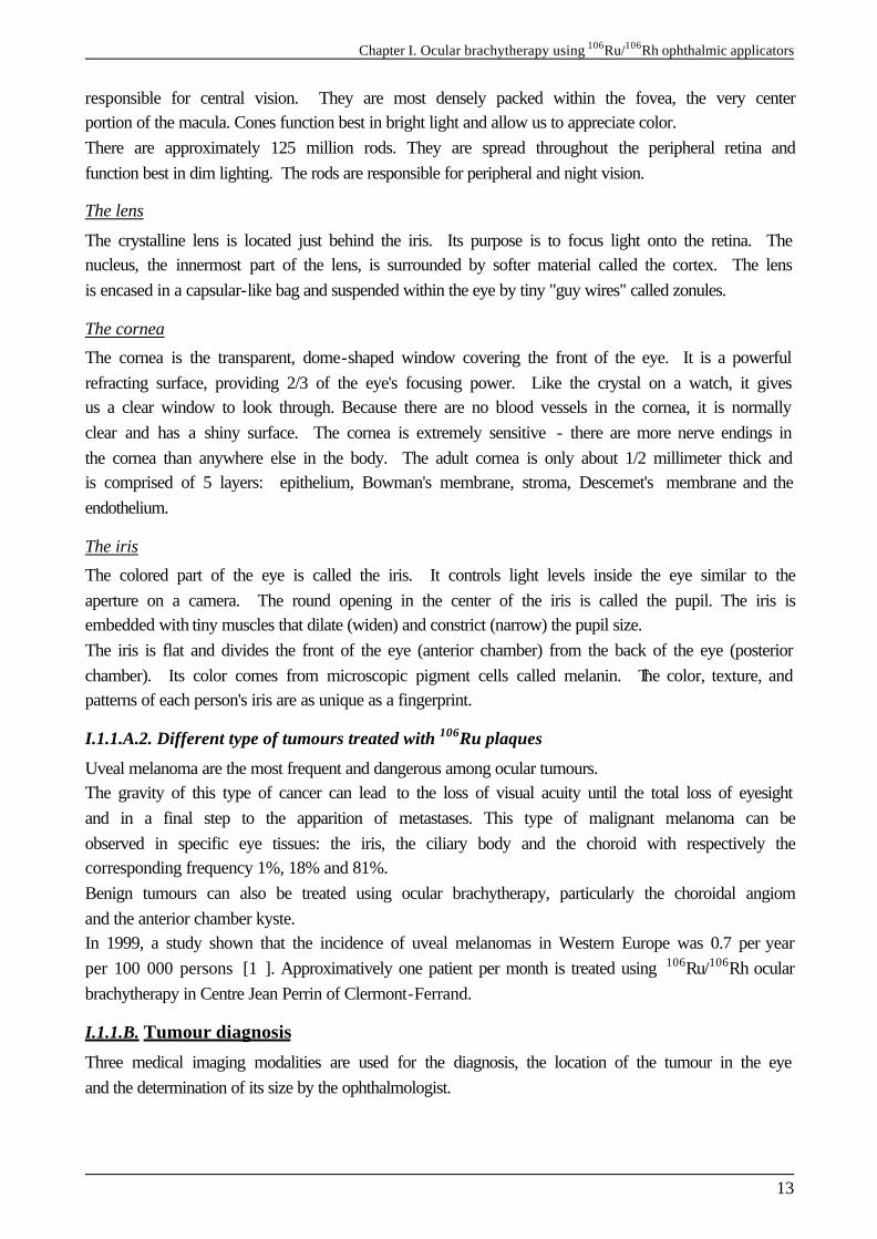
I.1.1.B.1. Photography
There are two types of special photographs ophthalmologists use to assist in diagnosis: fluorescein angiography and fundus photographs. § In fluorescein angiography, a special dye is injected into a vein in the arm. As the dye passes
through the blood vessels in the back of the eye, this allows for a view of the circulation of the retina and the layers beneath the retina, highlighting any abnormalities.
§ The fundus of the eye includes the retina, macula, fovea, optic disc and retinal vessels. In fundus photography, the inner lining of the eye is photographed with specially designed cameras through the dilated pupil. This is a non-invasive and painless procedure that produces a sharp view of the retina, the optic nerve and the retinal vessels.
Figure I- 2: Fundus of patient’s eye
Figure I- 3: Fundus image of a choroidal melanoma
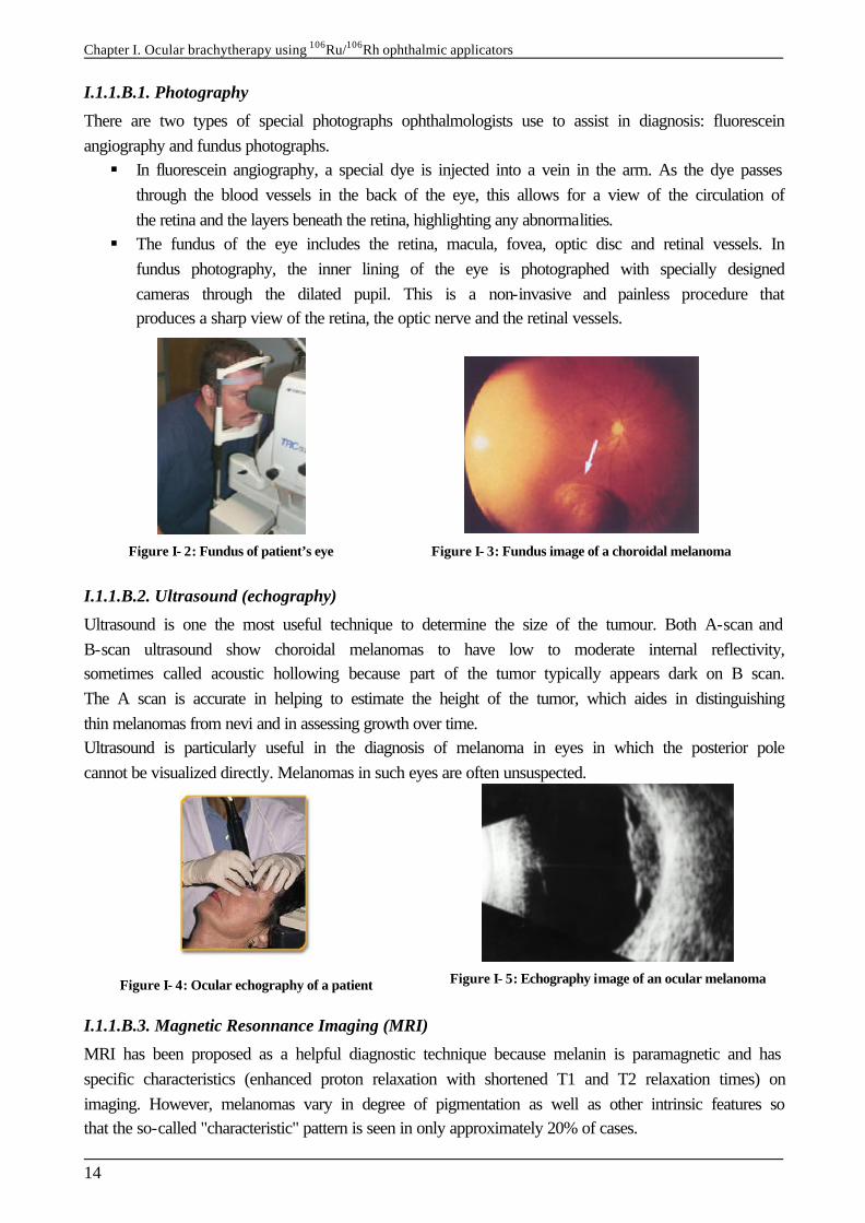
I.1.1.B.2. Ultrasound (echography)
Ultrasound is one the most useful technique to determine the size of the tumour. Both A-scan and B-scan ultrasound show choroidal melanomas to have low to moderate internal reflectivity, sometimes called acoustic hollowing because part of the tumor typically appears dark on B scan. The A scan is accurate in helping to estimate the height of the tumor, which aides in distinguishing thin melanomas from nevi and in assessing growth over time. Ultrasound is particularly useful in the diagnosis of melanoma in eyes in which the posterior pole cannot be visualized directly. Melanomas in such eyes are often unsuspected.
Figure I- 4: Ocular echography of a patient
Figure I- 5: Echography image of an ocular melanoma
I.1.1.B.3. Magnetic Resonnance Imaging (MRI)
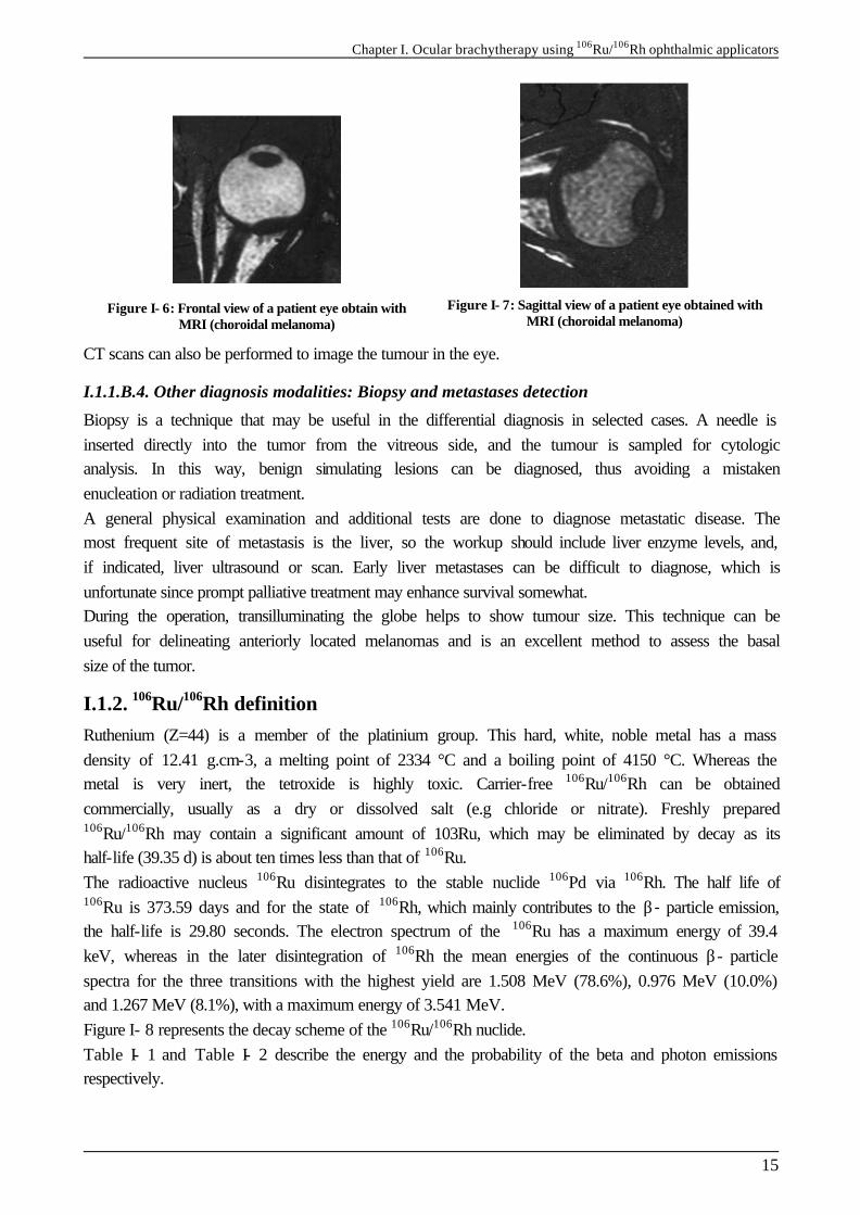
MRI has been proposed as a helpful diagnostic technique because melanin is paramagnetic and has specific characteristics (enhanced proton relaxation with shortened T1 and T2 relaxation times) on imaging. However, melanomas vary in degree of pigmentation as well as other intrinsic features so that the so-called "characteristic" pattern is seen in only approximately 20% of cases.
Chapter I. Ocular brachytherapy using 106Ru/106Rh ophthalmic applicators
15
Figure I- 6: Frontal view of a patient eye obtain with MRI (choroidal melanoma)
Figure I- 7: Sagittal view of a patient eye obtained with MRI (choroidal melanoma)
CT scans can also be performed to image the tumour in the eye.
I.1.1.B.4. Other diagnosis modalities: Biopsy and metastases detection
Biopsy is a technique that may be useful in the differential diagnosis in selected cases. A needle is inserted directly into the tumor from the vitreous side, and the tumour is sampled for cytologic analysis. In this way, benign simulating lesions can be diagnosed, thus avoiding a mistaken enucleation or radiation treatment. A general physical examination and additional tests are done to diagnose metastatic disease. The most frequent site of metastasis is the liver, so the workup should include liver enzyme levels, and, if indicated, liver ultrasound or scan. Early liver metastases can be difficult to diagnose, which is unfortunate since prompt palliative treatment may enhance survival somewhat. During the operation, transilluminating the globe helps to show tumour size. This technique can be useful for delineating anteriorly located melanomas and is an excellent method to assess the basal size of the tumor.
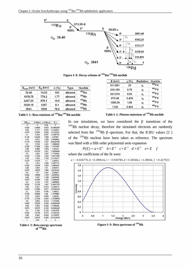
I.1.2. 106Ru/106Rh definition Ruthenium (Z=44) is a member of the platinium group. This hard, white, noble metal has a mass density of 12.41 g.cm-3, a melting point of 2334 °C and a boiling point of 4150 °C. Whereas the metal is very inert, the tetroxide is highly toxic. Carrier-free 106Ru/106Rh can be obtained commercially, usually as a dry or dissolved salt (e.g chloride or nitrate). Freshly prepared 106Ru/106Rh may contain a significant amount of 103Ru, which may be eliminated by decay as its half-life (39.35 d) is about ten times less than that of 106Ru. The radioactive nucleus 106Ru disintegrates to the stable nuclide 106Pd via 106Rh. The half life of 106Ru is 373.59 days and for the state of 106Rh, which mainly contributes to the β- particle emission, the half-life is 29.80 seconds. The electron spectrum of the 106Ru has a maximum energy of 39.4 keV, whereas in the later disintegration of 106Rh the mean energies of the continuous β- particle spectra for the three transitions with the highest yield are 1.508 MeV (78.6%), 0.976 MeV (10.0%) and 1.267 MeV (8.1%), with a maximum energy of 3.541 MeV. Figure I- 8 represents the decay scheme of the 106Ru/106Rh nuclide. Table I- 1 and Table I- 2 describe the energy and the probability of the beta and photon emissions respectively.
Chapter I. Ocular brachytherapy using 106Ru/106Rh ophthalmic applicators
16
Figure I- 8: Decay scheme of 106Ru/106Rh nuclide
Table I- 1: Beta emisions of 106Ru/106Rh nuclide
Table I- 2: Photon emissions of 106Rh nuclide
Table I- 3: Beta energy spectrum of 106Rh
In our simulations, we have considered the β transitions of the 106Rh nuclear decay, therefore the simulated electrons are randomly selected from the 106Rh β-spectrum. For that, the ICRU values [2 ] of the 106Rh nucleus have been taken as reference. The spectrum was fitted with a fifth order polynomial serie expansion
5 4 3 2( )P E a E b E c E d E e E f= × + × + × + × + × + where the coefficients of the fit were:
0.026776, 0.290614, 0.930780, 0.38568, 1.49044, 0.427923a b c d e f= − = = − = = =
Figure I- 9: Beta spectrum of 106Rh
Chapter I. Ocular brachytherapy using 106Ru/106Rh ophthalmic applicators
17
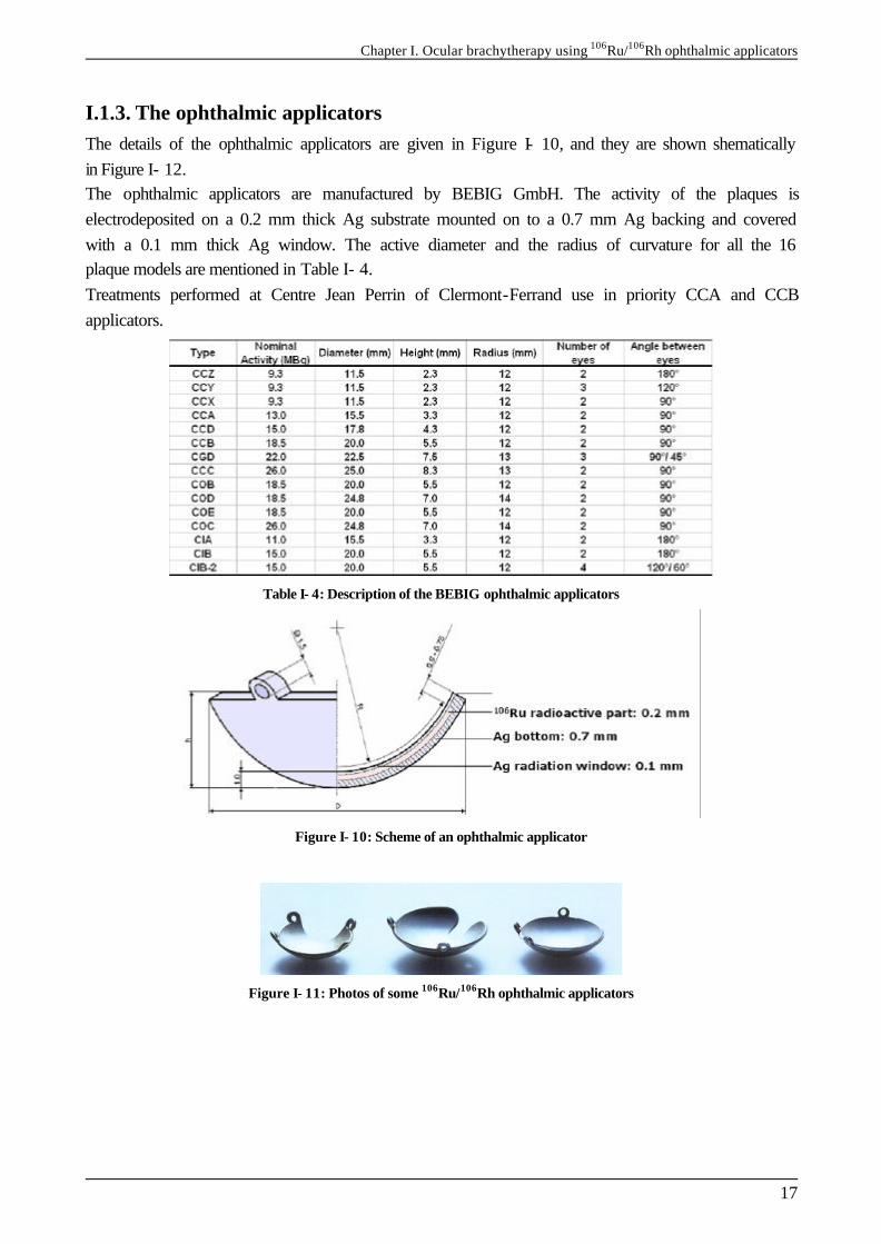
I.1.3. The ophthalmic applicators The details of the ophthalmic applicators are given in Figure I- 10, and they are shown shematically in Figure I- 12. The ophthalmic applicators are manufactured by BEBIG GmbH. The activity of the plaques is electrodeposited on a 0.2 mm thick Ag substrate mounted on to a 0.7 mm Ag backing and covered with a 0.1 mm thick Ag window. The active diameter and the radius of curvature for all the 16 plaque models are mentioned in Table I- 4. Treatments performed at Centre Jean Perrin of Clermont-Ferrand use in priority CCA and CCB applicators.
Table I- 4: Description of the BEBIG ophthalmic applicators
Figure I- 10: Scheme of an ophthalmic applicator
Figure I- 11: Photos of some 106Ru/106Rh ophthalmic applicators

Chapter I. Ocular brachytherapy using 106Ru/106Rh ophthalmic applicators
18
Figure I- 12: 16 types of Ru-106 ophthalmic plaques. The radioactive area is marked hatched.
I.1.4. Dose prescription and treatment efficacy
I.1.4.A. The Collaborative Ocular Melanoma Study (COMS)
In 1986, a COMS [3 ] sponsored by the National Eye Institute of the National Institute for Health among which 40 clinical centres of the United States and Canada participate, elaborate a prospective study in United states. The goal was to study the efficacy of the ocular brachytherapy treatments versus enucleation for the patient survival and the apparition of cancer metastasis. Enrollment of patients with ciliary body or choroidal melanoma began in 1987. Patients have been sorted into three groups: those with small, medium, and large tumors. Those with small tumors (up to 3 mm in elevation) are observed for tumor growth; if growth is sufficient to place the tumor in the medium group and if the patient remains eligible and willing, the eye is randomized for treatment. Patients with medium tumors (those between 3 mm and 8 mm in thickness and up to 16 mm in largest basal diameter) are randomized to either enucleation or plaque irradiation with iodine 125. Nearly 1200 patients have been enrolled in this arm of the study. Large tumors (greater than 8 mm in elevation and 16 mm in basal diameter) are randomized to receive external irradiation or no irradiation before standard enucleation. The cutoff between medium and large tumors was changed from 8-mm elevation to 10-mm elevation partway through the recruitment period. Before enrollment closed in 1994, 1003 patients were enrolled in this arm of the study. Part of the purpose of the COMS is to assess the natural history of the tumor in order to design effective management and also to evaluate therapy in a nonbiased fashion. Also, the study includes assessment of quality of life as well as vision retention in patients whose tumors are irradiated. As with other multicenter trials, one objective is to standardize observation and treatment criteria so that patients from different institutions can be compared. Developing standardized criteria is the only way we will be able to obtain sufficient data on a large enough group of patients to draw valid conclusions about natural history and treatment. A weakness of the study is that external charged particle treatment was not included. Also, there is no plan to compare efficacy of different plaque isotopes.

Chapter I. Ocular brachytherapy using 106Ru/106Rh ophthalmic applicators
19
More than a decade has passed since recruitment for the COMS began. Some preliminary results have been published recently, and one report confirms the very high accuracy rate of clinical diagnosis. Report No. 18 refers to I-125 Brachytherapy for Medium Choroidal Melanoma. No report has been written yet concerning 106Ru/106Rh brachytherapy.
I.1.4.B. Treatments using 106Ru/106Rh ophthalmic applicators
In Europe, Lommatzcsh pionneered the treatment of uveal melanomas in 1964 using ruthenium applicators, introducing these beta-emitting nuclides with directives for treatment [4 ][5 ][6 ][7 ]. As his results were good, many centres in Europe strated to use these applicators in the late 1970s and early 1980s [8 ][9 ][10 ][11 ][12 ][13 ][14 ]. A study performed in the Netherlands between 1984 and 1995 [1 ] explains the results of the treatment of 101 patients with 106Ru/106Rh ophthalmic applicators. It was demonstered that the tumour prominence and the given top dose were correlated strongly with the treatment outcome. 93.9 % of the patients were treated successfully resulting in a clinically complete remission in 62.6% whereas 31.3% kept a stable disease. It was shown that at a tumour top dose < 120 Gy five out of 22 tumours (23%) failed to respond, whereas at ≥ 120 Gy treatment only one out of 77 tumours did not respond, indicating that the top dose has to be at least 120 Gy. Müller et al. [15 ]and Pötter et al. [16 ] used a top dose of 150 Gy to obtain comparable results. A high success rate is also of vital importance as treatment failures are associated with a 2- to 3-fold increase in the rate of occurences of metastases [4 ]. The visual acuity is also of great importance for the patient’s quality of life. The Netheralnds study shown that a useful visual acuity of ≥ 0.3 was preserved in 51.5% of the 99 patients and visual acuity > 0.5 in 42.4% of the patients. Furthermore, a final visual acuity > 0.5 was found in 22.7% of the patients by Lommatzsch et al. [5 ] and in 27% by Pötter at al.[16 ]. It has been demonstered that the visual outcome after irradiation was better for peripherally than for centrally located tumours. The main reason for loss of central vision is radiation retinopathy in the macular area. The macular capillaries are highly sensitive to radiation and may be damaged by a low dose of 11-17 Gy [17 ][18 ]. An application of beta sources is the treatment of choroidal melanoma and retinoblastoma. These malignant diseases are treated with concave ruthenium plaques that can be stitched to the eye. At low dose rate the tumor is irradiated during a period varying from two up to fourteen days, depending on the activity of the source. The highenergy beta emitter ruthenium is used because tumor thickness can be up to 10 mm. Because the largest part of the absorbed dose is deposited in the first 10 mm from the source surface, and most tumors are situated at the posterior side of the eyeball, the absorbed dose to the lens usually is limited. The prescribed dose for treating choroidal melanoma is typically 80-120 Gy at the apex of the tumor. This is, however, limited by the surface dose that should not exceed 1000 Gy. In the literature the use of strontium sources for treatment of eye melanoma has also been reported [19 ]. Of all eye melanoma, uveal melanoma has the highest (yearly) incidence with six out of one million people. Over a period of 15 years the overall survival rate is estimated to be about 48% and the cumulative local treatment failure is 37%. Ciliar body melanoma (near the iris) and melanoma close to the optical nerve require use of applicators with a special shape.
Chapter I. Ocular brachytherapy using 106Ru/106Rh ophthalmic applicators
20
I.1.4.C. Other radiotherapy and brachytherapy treatments
I.1.4.C.1. Ocular brachytherapy using 125I ophthalmic plaques
COMS-type gold seeds carriers typically can be ordered in 5 sizes in 12-20 mm diameters. 125I rice-sized radioactive seeds are purchased and glued into the eye-plaque or seed carrier. The gold of the eye-plaque will block more than 99% of the radiation to the back and sides, creating a directional source. The active surface (facing us) is sewn onto the eye beneath the base of the intraocular tumor (just like it is done for 106Ru plaques). 125I is a low energy gammas emitter, the energies of the gamma rays generated are 27.202 keV (40.6 %), 27.472 keV (75.7 %), 30.98 keV (20.2 %), 31.71 keV (4.39 %) and 35.492 keV (6.68 %). Comparative study have been performed between the both brachytherapy using 125I seeds and 106Ru.
Figure I- 13: COMS iodine-125 ophthalmic applicators
Figure I- 14: Iodine-125 seeds in a COMS ophthalmic applicator.
Figure I- 15: Encapsulation of the iodine-125 seeds in a COMS applicator
With the 106Ru, Lommatzsch recomands 80-100 Gy at the top of the tumour with a dose rate of 5-10 Gy/h. With the iodine 125, by following the COMS protocol, for tumours of 3 to 5 mm in thickness, it is suitable to deliver 100 Gy at 5 mm in depth with a dose rate between 0.5 and 1.25 Gy/h to this point. Biological effects of such treatments have been compared in a lot of publications. We will refer here to the work performed at Centre Jean Perrin in collaboration with the ophthalmological clinic of the CHU G. Montpied of Clermont-Ferrand [20 ]. In that study, rabbit eyes have been irradiated with a CCZ ophthalmic plaques and with COMS iodine applicators of 12 mm in diameter. At 1 mm in depth the total dose deposited are comparable (317,1 Gy for 106Ru ophthalmic plaques and 326,9 Gy for iodine plaques), it is also the case for dose rate (3.07 Gy/h and 2.34 Gy/h respectively). The dose deposited is different for the both irradiation. High dose gradient from 106Ru plaques implies that the decreasing of the dose is very blunt, whereas for the iodine irradiation the decreasing of the dose is progressive (at 9mm far from the plaque, 6,6 Gy are delivered with the ruthenium-106 and 40,7 Gy with the iodine-125). The more important lesions have been observed using ruthenium-106 plaques whereas the dose delivered are lower for iodine-125. One year after the irradiation, irreversible lesions of the retina and optic nerve have been observed with the ruthenium-106 plaques whereas only few lesions of the external retina layer were observed.
Chapter I. Ocular brachytherapy using 106Ru/106Rh ophthalmic applicators
21
In clinical routine, iodine-125 plaques are used for larger tumors (thicknesses ranging from 6.5 mm to 11 mm). Those plaques show a dose fall-off factor of 2 per 4-5 mm water. For 100 Gy at the apex of an 8 mm tumor, the average sclera dose is 400 Gy, a value which is well tolerated. It has been reported that severe complications at neighboring structures overcame with iodine-125 plaque therapy [21 ][22 ]. For the tumour located in the posterior part of the eye, this treatment implicates a significant risk of retinopathy or opticus radiopathy. For large tumors, the necessity of applying a sufficient apex dose increases the risk to irradiate soft tissues at higher dose in the eye. Improvements on the plaque were done to limit the side effects during the irradiation. X-ray fluorescent foils were introduced into the applicator design (above or below the seeds depending on the backscatter or transmitted radiation want to be modified). The foils absorbed the photons of iodine-125 and emitted characteristic energy x-rays (15.8 keV for zirconium foil). The increasing cross-section of the photoelectric effect for these lower energies reduced the absorption lengths, causing a steeper dose fall-off. The dose distributions were then similar to those obtained with 103Pd radionuclide. Despite those modifications, it has been noticed that the iodine-125 plaques were not optimal for the treatments of the tumour in the range from 6.5 mm to 9 mm. It appeared also that dose to radiosensitive tissue in the eye remained high to preserve healthy tissues. Initial mortality findings published in 2001 (COMS Report No. 18) showed that survival rates for radiation therapy (I-125 brachytherapy) and enucleation (removal of the eye) are about the same. The five-year survival rate of patients who were treated with either radiation therapy or eye removal was 82 percent, considerably better than the 70 percent five-year survival rate that had been projected when the study was designed in 1985. Compared to immediate loss of vision when the eye is removed, eyes treated with radiation steadily lost vision gradually, with 63 percent having visual acuity of 20/200 or worse by three years after treatment (COMS Report No. 16).
I.1.4.C.2. Ocular brachytherapy using bi-nuclide radioactive ophthalmic applicators
Eye plaque brachytherapy with the radioactive nuclides 106Ru/106Rh and 125I has been established as an other standard treatment modality for years. In order to optimize the spatial dose distribution, the characteristics of both nuclides are exploited. The goal is to obtain a dose sparing effect at large distances contrary to iodine-125 plaques and give tolerable doses within the target volume and to the sclera for which the dose shouldn’t overlapp 1200 Gy during all the treatment. The bi-nuclide applicator consists of three elements. The design is based on a carrier calotte made of a gold alloy with lateral shielding rings and two fixation eyes for suturing the plaque onto the bulbus. In this calotte a 106Ru/106Rh plaque BEBIG type without fixation eyes is inserted and fixed with some silicone. The third part is a silicone inset with 8-12 symmetrically arranged iodine seeds, Amersham type 6711. However the dosimetry of a bi-nuclide applicator is difficult because the beta radiation of 106Ru has to pass through the silicone layer and the iodine seeds and because the iodine radiation is influenced by the silver 106Ru plaque (x-ray fluorescence effect), it has been shown that this type of applicators offers a considerable dose reduction at radiosensitive structures within the eye. For tumour thicknesses comprise between 6.5 and 9 mm, a bi-nuclide plaque reaches 40-80% of the dose deposition of an iodine-125 plaque at the opposite point. For tumours of 6.5 mm a sclera dose reduction of 20-30% can be observed compared to 106Ru/106Rh plaques. The gain of such plaque
Chapter I. Ocular brachytherapy using 106Ru/106Rh ophthalmic applicators
22
comparing to iodine plaque is that the dose at the lens decreases much faster for the bi-nuclide than for iodine-125 due to the steep dose fall-off of 106Ru/106Rh. For tumours of thicknesses of 10 mm and more, the application of bi-nuclide plaques is not advantageous.
I.1.4.C.3. The protontherapy
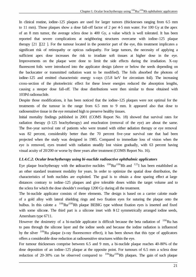
For specific location of choroidal melanoma and for high tumour thicknesses, the protontherapy is prefered to the brachytherapy.
Figure I- 16: Ocular nozzle and proton beam line schema of the Nice hadrontherapy platform.
Figure I- 17: The ocular nozzle
The cyclotron provides 65 MeV protons. The accelerator is a fixed frequency 25 MHz isochronous cyclotron with a peak voltage of 50 kV. Negative hydrogen ions are produced by an external source, axially injected and accelerated to 65 MeV. They are then extracted by a 60×10- 6 g cm- 2 carbon stripping foil and exiting protons are transported down the beam line to the treatment room. The main components of the ocular beam line are presented in Figure I- 16 and Figure I- 17. The incoming proton beam is completely defocused after the achromatic focal point of the last 90° bending magnet (M4), regarded as the source point for calculations, before reaching a 5×10- 3 -cm-thick tantalum foil. These elements act together as a single scatterer providing 12 m behind away, a flat beam at the irradiation point. In the vacuum part, upstream from the ocular nozzle, the beam aperture is limited to 5 cm diameter by two graphite collimators. Afterwards, decreasing the collimator size from 5 to 4.5 and finally 3.4 cm, only the central part of the beam is selected. The ocular nozzle part of the beam line is composed two brass collimators opened to a 5 cm diameter; a kapton foil 1.3×10⁻² cm thick, sparing vacuum to air, also closes its upstream extremity. This empty box holds the range shifter and the Lucite propeller, which are used to adapt the incoming proton beam in range and modulation. The following part contains two monitor chambers made of aluminized mylar, two 4.5 cm brass collimators, and an exiting copper nozzle of 3.4 cm internal diameter, which supports the final individual brass patient collimator. In the clinical situation spread out Bragg peaks (SOBP) are required to provide homogeneous irradiation in depth, z. The corresponding depthdose curve D(z) is obtained by adding the weighted contribution of individual (i) reduced Bragg peak curves Di(z) achieved by the introduction of a thickness of Lucite t,

Chapter I. Ocular brachytherapy using 106Ru/106Rh ophthalmic applicators
23
0
( ) ( )n
i ii
D z p D z=
= ∑
t=ns where pi represents the weighting factor of the reduced peak i, n is the total number of peaks needed to achieve a defined length of SOBP t, z is the depth of irradiation, and s is the thickness step of reducing material equal to 8×10⁻² cm. The irradiation is preceded by the location of the tumour and the positionning of tantale clips sutured to the sclera. 60 Gy are delivered to the tumour in four fractions and four days. A security margin of 2.5 mm around the tumour is fixed. The enucleation rate is about 10 % after a protontherapy treatment.
I.2. QUALITY CONTROL AND DOSE MEASUREMENTS
I.2.1. Measurements Physical measurements of dose distribution on ophthalmic applicators are difficult because the dose gradient of 106Ru/106Rh plaques is very high on a region of therapeutic interest which is less than 25 mm. This requires very small detectors that have to be positionned very precisely whith a good determination of the effective point of measurement. In the following sections, detectors for absorbed dose measurements on beta sources are described with a special emphasis on radiochromic films used particularly in the quality control of the source and the plastic scintillators use for the dose distribution measurement and calibration thanks to their small design.
I.2.1.A. Absolute calibration of beta sources: the extrapolation chamber
Extrapolation chambers are considered as the standard device for the dosimetry of beta particle sources. The extrapolation chamber allows the ionization volume to be varied to a vanishingly small amount. The US standards laboratory NIST uses such a chamber as a primary standard for the calibration of sealed beta sources [23 ]. Recently, at the NMi a primary standard was built for the dosimetry of clinical sealed beta sources, based on the principle of the extrapolation chamber. The extrapolation chamber is a parallel plate ionization chamber with variable air volume. The ionization volume is determined by the distance between the parallel plates and by the effective area of the central electrode. The central electrode, surrounded by a guard electrode, is situated at the center of one of the parallel plates. The other parallel plate is the entrance window of the ionization chamber. The central and guard electrodes are constructed from an electrically conductive and water equivalent plastic resembling polystyrene, called D400 (Standard Imaging, Middleton, WI, USA). The ionization current collected by the central electrode is measured at different plate distances and extrapolated to zero air volume, in order to approximate the ideal Bragg-Gray conditions. The extrapolated ionization current is a measure for the absorbed dose to air, taking into account the geometrical conditions and the materials used to construct the extrapolation chamber. The absorbed dose rate to water ( WD
•) can be determined from the ionization current measurements
using Bragg-Gray theory. The extrapolation chamber requires no radiation calibration but the area of the collecting electrode is a major limitation in the absolute accuracy of the measurements.
Chapter I. Ocular brachytherapy using 106Ru/106Rh ophthalmic applicators
24
I.2.1.B. Radiochromic film (RCF)
Radiochromic film has turned into the most widely used method for verification of the uniformity of beta sources, it can also be used to measure dose deposited by sources in solid phantoms. GafChromicTM (ISP Technologies Inc., Wayne, NJ, USA) is available in single and double layer versions. A thin layer of almost colorless emulsion is coated on a Polyethylene TerePhthalate (PTP) backing, forming a single or double sandwich of layers. The sensitive emulsion layer is between 7 and 40 µm thick, depending on the type of film. The total thickness can be between 0.1-0.3 mm. The sensitive layer turns blue upon irradiation and does not require post-irradiation processing. The sensitivity of most films is low, so that an absorbed dose of at least tens of Grays is needed. Films can be calibrated for absolute measurements [24 ]. The energy dependence is low in the energy range relevant for clinical beta sources (100 keV - 2 MeV, [42]). A major limitation of the radiochromic film is the variation in thickness of the sensitive layer resulting in a non-uniform response (up to 15% for MD55-2 [43]). Because of these variations, the measurement uncertainty is estimated to be about 7.5% for the absorbed dose. For absolute measurements a delay of at least 24 hours needs to be taken into account to minimize effects of incomplete film development. Uniformity information can be quantified by film densitometry [25 ]. Uniformity variations of more than ~ 10% can be detected (qualitatively) by the eye. In the literature radiochromic film measurements are described for both ophthalmic [26 ][27 ] and intravascular [24 ][28 ] sources. RCF will be used to measure dose deposited in a solid water phantom for some ophthalmic applicators. MD55-2 radiochromic films are used for the dosimetry of 106Ru/106Rh plaques. They support a dose range from 3 to 100 Gy, of 278 µm in thickness with two sensitive layers.
I.2.1.B.1. Radiochromic film calibrations
Because radiochromic film is tissue equivalent over a broad energy range, it was calibrated with a regular 6 MV photon beam of a linear accelerator. All measurements were performed at the dose maximum of the PDD. A fit was performed according to Equation I- 2, in which Dw is the absorbed dose to water and OD is the optical density according to the red channel of the RGB (Red-Green-Blue) based TIF file. This channel has the strongest correlation with darkening of the film. The OD was calculated using Equation I- 1. T in this equation is transmittance, expressing the ratio of the pixel value at a given absorbed dose and the pixel value of film that was not irradiated. 10 log( )OD T= − Equation I- 1
2 31 2 3wD a bOD b O D b OD= + + + Equation I- 2
The calibration curve is unique for each densitometer-film combination. Based on the specific shape of the curve a choice can be made for a 2nd or 3rd order polynomial. The uncertainty shown by the error bars is a combination of film non-uniformity and scanner noise. A flatbed transmission scanner is currently used for film densitometry (EPSON Expression 1680). This scanner is used in 3×16 bit mode with 12 bit colour depth. The films are scanned at 300 dpi (pixel size 0.08×0.08 mm2).
Chapter I. Ocular brachytherapy using 106Ru/106Rh ophthalmic applicators
25
I.2.1.C. Thermoluminescence dosimeters (TLD)
Although most hospitals make use of TLDs for dosimetry, dedicated TLDs are required for measurements on beta sources [28 ][29 ][30 ][31 ]. The most important property of these TLDs is their small size (as small as 0.1 mm thickness and 1 mm diameter for the active volume), which makes them suitable for determining the spatial distribution of the dose around a source. Due to their small size and water-equivalence these TLDs give only very small distortions of the radiation field. The TLDs are usually embedded in a solid phantom. Readout is performed afterwards by heating the TLDs and measuring the amount of light with a photomultiplier. Calibration is carried out in a clinical MeV electron beam or with a calibrated beta source. TLDs can also be used for measurements on concave ophthalmic applicators [32 ][33 ][34 ]. The estimated standard uncertainty (1σ) is between 8-10% depending on knowledge of precise phantom dimensions and TLD characteristics [29 ].
I.2.1.D. Alanine pellets
Dosimetry with alanine is based on the relative and non-destructive measurement of stable free radicals produced by radiation [29 ][35 ]. These dosemeters are read out with an X-band Electron Paramagnetic Resonance (EPR) spectrometer with a scan range of 0-2 mT. Advantages of the detector are the linear response and absence of energy dependence. The detector has a diameter of about 5 mm and a thickness of about 1 mm. These dimensions also determine the sensitive volume and therefore are a disadvantage of the method. Another disadvantage is the low sensitivity, because the EPR signal is very weak. An estimated standard uncertainty of 5-7% (1σ) can be expected in the region between 10-20 Gy [29 ].
I.2.1.E. Scintillator
Plastic scintillators were first introduced for dosimetry of brachytherapy sources at the University of Essen [36 ]. Plastic scintillator probes have a homogeneous sensitive volume with approximate water equivalence in density and atomic composition. Due to their high sensitivity, scintillation detectors can be designed with probe volumes as small as 1 mm3 or even less. Scintillation detectors offer the great advantage that they can be read out directly. The detector is based on light being generated in the plastic scintillator volume. The scintillation light is detected with a photomultiplier through an optical fiber that have to give sufficient transmission of scintillation light and the simultaneous Cerenkov compensation. The Essen plastic scintillator has a thickness of 0.4 mm and a diameter of 1 mm. Measurements on ophthalmic applicators (125I and 106Ru/106Rh) showed a contribution of Cherenkov light of no more than 2%. The OptidosTM is a commercial version of this system developed by PTW (PTW Freiburg GmbH, Freiburg, Germany). The plastic scintillator has a detection volume of 0.8 mm3 (1 mm thickness and 1 mm diameter) and an outer diameter of 5.2 mm, in the last years plastic scintillator size was reduced to 1 mm in diameter and 0.5 mm in height (BEBIG calibration). The system has no blind fiber for Cherenkov compensation. Measurements need to be accompanied by check source measurements to correct for changes in the detector sensitivity. The estimated standard uncertainty (1σ) is 3% for relative dosimetry with the larger plastic scintillator without Cherenkov compensation and 7% for the smaller scintillator with Cherenkov compensation [29 ].
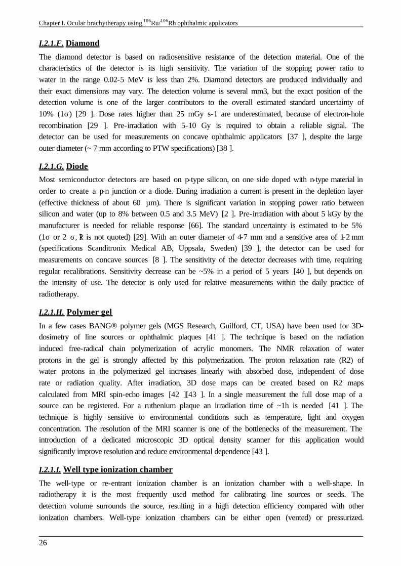
Chapter I. Ocular brachytherapy using 106Ru/106Rh ophthalmic applicators
26
I.2.1.F. Diamond
The diamond detector is based on radiosensitive resistance of the detection material. One of the characteristics of the detector is its high sensitivity. The variation of the stopping power ratio to water in the range 0.02-5 MeV is less than 2%. Diamond detectors are produced individually and their exact dimensions may vary. The detection volume is several mm3, but the exact position of the detection volume is one of the larger contributors to the overall estimated standard uncertainty of 10% (1σ) [29 ]. Dose rates higher than 25 mGy s-1 are underestimated, because of electron-hole recombination [29 ]. Pre-irradiation with 5-10 Gy is required to obtain a reliable signal. The detector can be used for measurements on concave ophthalmic applicators [37 ], despite the large outer diameter (~ 7 mm according to PTW specifications) [38 ].
I.2.1.G. Diode
Most semiconductor detectors are based on p-type silicon, on one side doped with n-type material in order to create a p-n junction or a diode. During irradiation a current is present in the depletion layer (effective thickness of about 60 µm). There is significant variation in stopping power ratio between silicon and water (up to 8% between 0.5 and 3.5 MeV) [2 ]. Pre-irradiation with about 5 kGy by the manufacturer is needed for reliable response [66]. The standard uncertainty is estimated to be 5% (1σ or 2 σ, ??k is not quoted) [29]. With an outer diameter of 4-7 mm and a sensitive area of 1-2 mm (specifications Scanditronix Medical AB, Uppsala, Sweden) [39 ], the detector can be used for measurements on concave sources [8 ]. The sensitivity of the detector decreases with time, requiring regular recalibrations. Sensitivity decrease can be ~5% in a period of 5 years [40 ], but depends on the intensity of use. The detector is only used for relative measurements within the daily practice of radiotherapy.
I.2.1.H. Polymer gel
In a few cases BANG® polymer gels (MGS Research, Guilford, CT, USA) have been used for 3D-dosimetry of line sources or ophthalmic plaques [41 ]. The technique is based on the radiation induced free-radical chain polymerization of acrylic monomers. The NMR relaxation of water protons in the gel is strongly affected by this polymerization. The proton relaxation rate (R2) of water protons in the polymerized gel increases linearly with absorbed dose, independent of dose rate or radiation quality. After irradiation, 3D dose maps can be created based on R2 maps calculated from MRI spin-echo images [42 ][43 ]. In a single measurement the full dose map of a source can be registered. For a ruthenium plaque an irradiation time of ~1h is needed [41 ]. The technique is highly sensitive to environmental conditions such as temperature, light and oxygen concentration. The resolution of the MRI scanner is one of the bottlenecks of the measurement. The introduction of a dedicated microscopic 3D optical density scanner for this application would significantly improve resolution and reduce environmental dependence [43 ].
I.2.1.I. Well type ionization chamber
The well-type or re-entrant ionization chamber is an ionization chamber with a well-shape. In radiotherapy it is the most frequently used method for calibrating line sources or seeds. The detection volume surrounds the source, resulting in a high detection efficiency compared with other ionization chambers. Well-type ionization chambers can be either open (vented) or pressurized.
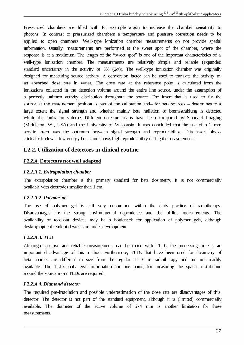
Chapter I. Ocular brachytherapy using 106Ru/106Rh ophthalmic applicators
27
Pressurized chambers are filled with for example argon to increase the chamber sensitivity to photons. In contrast to pressurized chambers a temperature and pressure correction needs to be applied to open chambers. Well-type ionization chamber measurements do not provide spatial information. Usually, measurements are performed at the sweet spot of the chamber, where the response is at a maximum. The length of the “sweet spot” is one of the important characteristics of a well-type ionization chamber. The measurements are relatively simple and reliable (expanded standard uncertainty in the activity of 5% (2σ)). The well-type ionization chamber was originally designed for measuring source activity. A conversion factor can be used to translate the activity to an absorbed dose rate in water. The dose rate at the reference point is calculated from the ionizations collected in the detection volume around the entire line source, under the assumption of a perfectly uniform activity distribution throughout the source. The insert that is used to fix the source at the measurement position is part of the calibration and– for beta sources – determines to a large extent the signal strength and whether mainly beta radiation or bremsstrahlung is detected within the ionization volume. Different detector inserts have been compared by Standard Imaging (Middleton, WI, USA) and the University of Wisconsin. It was concluded that the use of a 2 mm acrylic insert was the optimum between signal strength and reproducibility. This insert blocks clinically irrelevant low-energy betas and shows high reproducibility during the measurements.
I.2.2. Utilization of detectors in clinical routine
I.2.2.A. Detectors not well adapted
I.2.2.A.1. Extrapolation chamber
The extrapolation chamber is the primary standard for beta dosimetry. It is not commercially available with electrodes smaller than 1 cm.
I.2.2.A.2. Polymer gel
The use of polymer gel is still very uncommon within the daily practice of radiotherapy. Disadvantages are the strong environmental dependence and the offline measurements. The availability of read-out devices may be a bottleneck for application of polymer gels, although desktop optical readout devices are under development.
I.2.2.A.3. TLD
Although sensitive and reliable measurements can be made with TLDs, the processing time is an important disadvantage of this method. Furthermore, TLDs that have been used for dosimetry of beta sources are different in size from the regular TLDs in radiotherapy and are not readily available. The TLDs only give information for one point; for measuring the spatial distribution around the source more TLDs are required.
I.2.2.A.4. Diamond detector
The required pre-irradiation and possible underestimation of the dose rate are disadvantages of this detector. The detector is not part of the standard equipment, although it is (limited) commercially available. The diameter of the active volume of 2-4 mm is another limitation for these measurements.
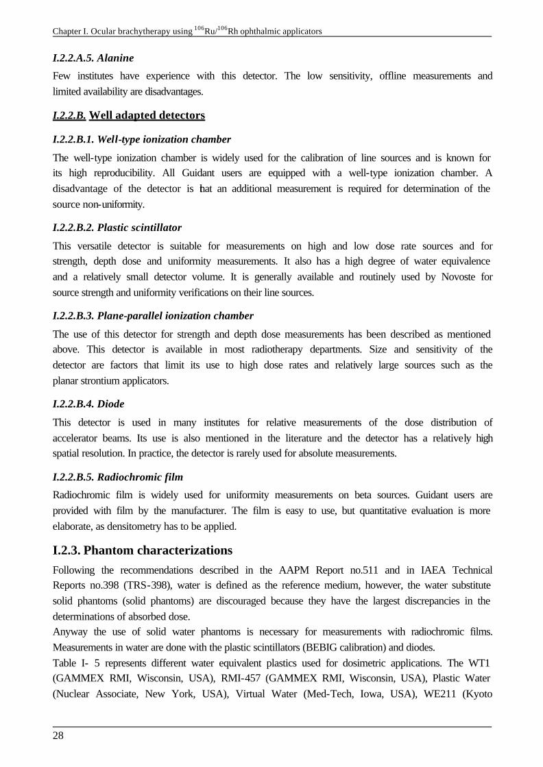
Chapter I. Ocular brachytherapy using 106Ru/106Rh ophthalmic applicators
28
I.2.2.A.5. Alanine
Few institutes have experience with this detector. The low sensitivity, offline measurements and limited availability are disadvantages.
I.2.2.B. Well adapted detectors
I.2.2.B.1. Well-type ionization chamber
The well-type ionization chamber is widely used for the calibration of line sources and is known for its high reproducibility. All Guidant users are equipped with a well-type ionization chamber. A disadvantage of the detector is that an additional measurement is required for determination of the source non-uniformity.
I.2.2.B.2. Plastic scintillator
This versatile detector is suitable for measurements on high and low dose rate sources and for strength, depth dose and uniformity measurements. It also has a high degree of water equivalence and a relatively small detector volume. It is generally available and routinely used by Novoste for source strength and uniformity verifications on their line sources.
I.2.2.B.3. Plane-parallel ionization chamber
The use of this detector for strength and depth dose measurements has been described as mentioned above. This detector is available in most radiotherapy departments. Size and sensitivity of the detector are factors that limit its use to high dose rates and relatively large sources such as the planar strontium applicators.
I.2.2.B.4. Diode
This detector is used in many institutes for relative measurements of the dose distribution of accelerator beams. Its use is also mentioned in the literature and the detector has a relatively high spatial resolution. In practice, the detector is rarely used for absolute measurements.
I.2.2.B.5. Radiochromic film
Radiochromic film is widely used for uniformity measurements on beta sources. Guidant users are provided with film by the manufacturer. The film is easy to use, but quantitative evaluation is more elaborate, as densitometry has to be applied.
I.2.3. Phantom characterizations Following the recommendations described in the AAPM Report no.511 and in IAEA Technical Reports no.398 (TRS-398), water is defined as the reference medium, however, the water substitute solid phantoms (solid phantoms) are discouraged because they have the largest discrepancies in the determinations of absorbed dose. Anyway the use of solid water phantoms is necessary for measurements with radiochromic films. Measurements in water are done with the plastic scintillators (BEBIG calibration) and diodes. Table I- 5 represents different water equivalent plastics used for dosimetric applications. The WT1 (GAMMEX RMI, Wisconsin, USA), RMI-457 (GAMMEX RMI, Wisconsin, USA), Plastic Water (Nuclear Associate, New York, USA), Virtual Water (Med-Tech, Iowa, USA), WE211 (Kyoto
Chapter I. Ocular brachytherapy using 106Ru/106Rh ophthalmic applicators
29
Kagaku, Kyoto, Japan), Polystyrene, Polymethyl Methacrylate (PMMA) and MixDP are commercially available materials.
Table I- 5: Water-equivalent plastics used for dosimetric measurements.
Figure I- 18, Figure I- 19 represent the NIST phantoms in WT1 plastic water used for the dosimetry of 106Ru/106Rh ophthalmic applicators using radiochromic films. Figure I- 20 shows an other phantom configuration used at the NYU Cornell Medical Center, RMI457 plastic was used. MD55-2 Gafchromic films of 278 µm in thickness are inserted between phantom slices to test the non-uniformity (see section I.3.1.c) of the source and make some dosimetric studies. An elaboration of a phantom in virtual water is under development at Laboratoire de Physique Corpusculaire in order to perform quality control on ophthalmic beta sources at Centre Jean Perrin.
Figure I- 18: NIST WT1 solid phantoms used for depth dose measurements.
Image courtesy of C. Soares, NIST, Washington DC
Figure I- 19: NIST WT1 solid phantom with different cap heights used for the concave
ophthalmic applicators.
Image courtesy of C. Soares, NIST, Washington DC
Figure I- 20: RMI457 solid water phantom and GAFCHROMIC MD-55 film,
Image courtesy of Samuel Trichter, NYU Cornell Medical Center, New York
Chapter I. Ocular brachytherapy using 106Ru/106Rh ophthalmic applicators
30
I.3. Quality control of ophthalmic applicators After the reception of ophthalmic sources, quality control on sources are highly recommended in order to check their uniformity and the dose distribution provided. Even if the sources are delivered with a calibration sheet provided by the manufacturer, it has been shown in the Report 14 of the Netherlands Commission on Radiation Dosimetry [44 ] that differences are observed by double checking the source strength and the non-uniformity of the sources.
I.3.1. Parameters to study
I.3.1.A. Average radius (R50)
The average radius (R50) is defined as the mean radius of the 50% isodose contour of a dose distribution in which 100% is given by the maximum absorbed dose. A precise description of how this radius can be calculated is given in the section on source non-uniformity (see below).
I.3.1.B. Source strength
The source strength of all planar and concave sources is defined as the dose rate at (r, z) = (0,1) mm following the recommendations of the ICRU report [45 ]. The IAEA [46 ] recommends using the same point but recognizes that performing measurements at these short distances is a difficult task. Effectively, the curvature of concave sources and minimum thickness of spacers limit the possibilities of performing measurements at 1 mm, even if detector dimensions are sufficiently small. The recommendation that is to determine the source strength at (r0, z0) = (0,2) mm has been followed by the BEBIG company in their measurements protocols, the reference dose rate is measured at r=0 and z=2 mm.
I.3.1.B.1. Source strength specification by manufacturer
BEBIG introduced a new standard in 2002 based on the NIST measurement protocol. Uncertainties of both old and new standards are specified. BEBIG is the only manufacturer that actually specifies activity and provides a conversion factor for the absorbed dose to water. Other manufacturers specify in a reference point in water.
I.3.1.C. Source non-uniformity
The source non-uniformity for eye applicators, as introduced in the ICRU report, is given by Equation I- 4:
max min( ) / 100%avgICRUU D D D• • •
= − × Equation I- 3
in which: UICRU = source non-uniformity (%), maxD
•= maximum absorbed dose rate, minD
•= minimum
absorbed dose rate, avgD•
= average absorbed dose rate. The report recommends that the non-uniformity should be determined at a specified depth over a specified area of the source. Although the principle can also be used for measurements with a larger detector such as a diode, this concept is especially suitable for scanned radiochromic films. The ICRU proposes to determine the non-uniformity at z = 1 mm depth, using 80% of R50. The calculation of the source non-uniformity is performed as follows:

Chapter I. Ocular brachytherapy using 106Ru/106Rh ophthalmic applicators
31
The maximum absorbed dose rate max maxD•
is determined. The pixels with 50% of max maxD
• are determined (for films, absorbed dose values are used, instead
of dose rate values). The coordinate of the field center (xc,yc) is determined through:
1 1
50 5050 501 1,
2 2
n mj ji i
c ci j
y yx xx y
n m
− +− +
= =
++ = =
∑ ∑ Equation I- 4
In which n is the number of rows and m is the number of columns with a dose rate larger than or equal to 50% of max maxD
•. The sign indicates the position with respect to the source center.
The average radius R50 can be calculated through:
( )2 250
1
1( 50 ) ( 50 )
q
c k c kk
R x x y yq =
= − + −
∑ Equation I- 5
in which q is the total number of 50% pixels. Finally, analogous to the concept for line sources, Equation I- 3 is applied, in which minD
•, maxD
•,
avgD•
are taken from the pixels with a distance smaller than 0.8R50 to (xc,yc). The ICRU recommends a maximum source non-uniformity UICRU of 20%. For concave sources the concept of non-uniformity can be applied in different ways: § in a concave surface parallel to the source surface, § in a plane perpendicular to the source axis.
Although uniformity measurements should preferably be performed parallel to the source surface, film measurements are only possible in a plane. In the literature, film measurements on concave ophthalmic sources are described in [29 ]. The concept of non-uniformity proposed by the ICRU has some disadvantages: § The non-uniformity does not give the maximum possible deviation from the source strength,
but only the difference between minimum and maximum. § The normalization is performed based on an average of the absorbed dose within the area of
interest and can therefore not be related directly to the source strength that is defined in a point on the axis.
I.3.1.D. Source asymmetry
It was decided by the NCS (Netherlands Commission on Radiation Dosimetry) in their report 14 to use a wider margin for the non-uniformity and to introduce an additional parameter for evaluating sources with respect to the asymmetry of the dose distribution. To quantify the asymmetry of the dose distribution of ophthalmic sources, the parameter for source asymmetry UAS is introduced: { }max minmax ( ) ( ) / ( ) 100%avgASU D r D r D r
• • • = − ×
Equation I- 6
In this expression the variation of the dose rate is calculated over a circle with a radius r. The maximum of this variation, with r ranging from zero to 0.8R50, determines the value of the asymmetry UAS. The asymmetry is defined parallel to the source surface. For concave sources, a film measurement in a plane may be used as an approximation of UAS.
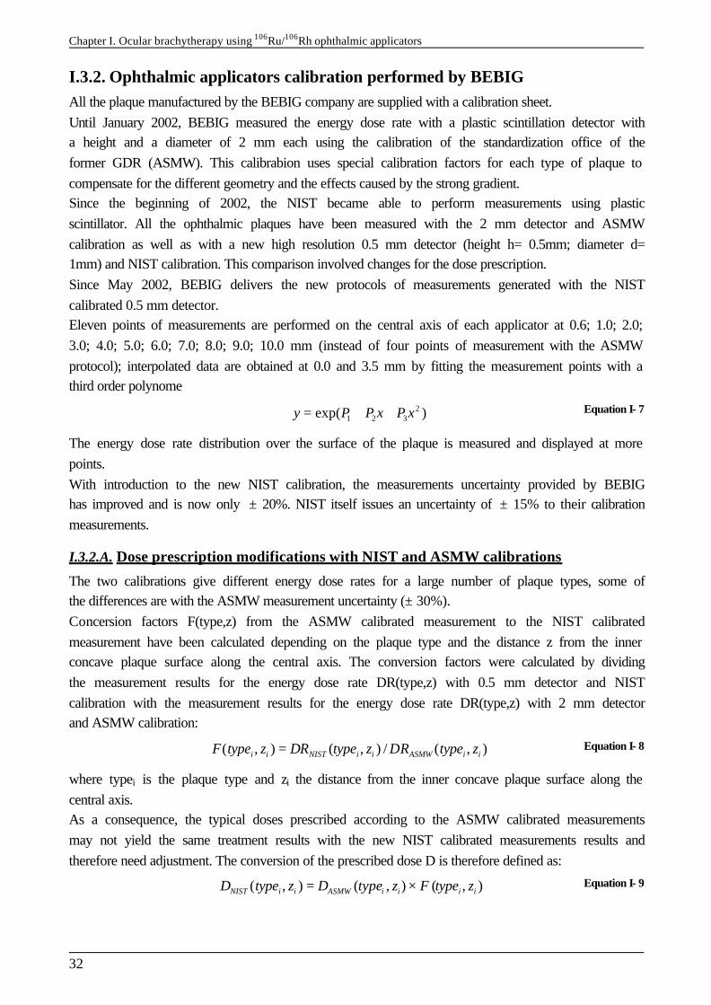
Chapter I. Ocular brachytherapy using 106Ru/106Rh ophthalmic applicators
32
I.3.2. Ophthalmic applicators calibration performed by BEBIG All the plaque manufactured by the BEBIG company are supplied with a calibration sheet. Until January 2002, BEBIG measured the energy dose rate with a plastic scintillation detector with a height and a diameter of 2 mm each using the calibration of the standardization office of the former GDR (ASMW). This calibrabion uses special calibration factors for each type of plaque to compensate for the different geometry and the effects caused by the strong gradient. Since the beginning of 2002, the NIST became able to perform measurements using plastic scintillator. All the ophthalmic plaques have been measured with the 2 mm detector and ASMW calibration as well as with a new high resolution 0.5 mm detector (height h= 0.5mm; diameter d= 1mm) and NIST calibration. This comparison involved changes for the dose prescription. Since May 2002, BEBIG delivers the new protocols of measurements generated with the NIST calibrated 0.5 mm detector. Eleven points of measurements are performed on the central axis of each applicator at 0.6; 1.0; 2.0; 3.0; 4.0; 5.0; 6.0; 7.0; 8.0; 9.0; 10.0 mm (instead of four points of measurement with the ASMW protocol); interpolated data are obtained at 0.0 and 3.5 mm by fitting the measurement points with a third order polynome
21 2 3exp( )y P P x P x= + + Equation I- 7
The energy dose rate distribution over the surface of the plaque is measured and displayed at more points. With introduction to the new NIST calibration, the measurements uncertainty provided by BEBIG has improved and is now only ± 20%. NIST itself issues an uncertainty of ± 15% to their calibration measurements.
I.3.2.A. Dose prescription modifications with NIST and ASMW calibrations
The two calibrations give different energy dose rates for a large number of plaque types, some of the differences are with the ASMW measurement uncertainty (± 30%). Concersion factors F(type,z) from the ASMW calibrated measurement to the NIST calibrated measurement have been calculated depending on the plaque type and the distance z from the inner concave plaque surface along the central axis. The conversion factors were calculated by dividing the measurement results for the energy dose rate DR(type,z) with 0.5 mm detector and NIST calibration with the measurement results for the energy dose rate DR(type,z) with 2 mm detector and ASMW calibration:
( , ) ( , ) / ( , )i i NIST i i ASMW i iF type z DR type z DR type z= Equation I- 8
where typei is the plaque type and zi the distance from the inner concave plaque surface along the central axis. As a consequence, the typical doses prescribed according to the ASMW calibrated measurements may not yield the same treatment results with the new NIST calibrated measurements results and therefore need adjustment. The conversion of the prescribed dose D is therefore defined as:
( , ) ( , ) ( , )NIST i i ASMW i i i iD type z D type z F type z= × Equation I- 9
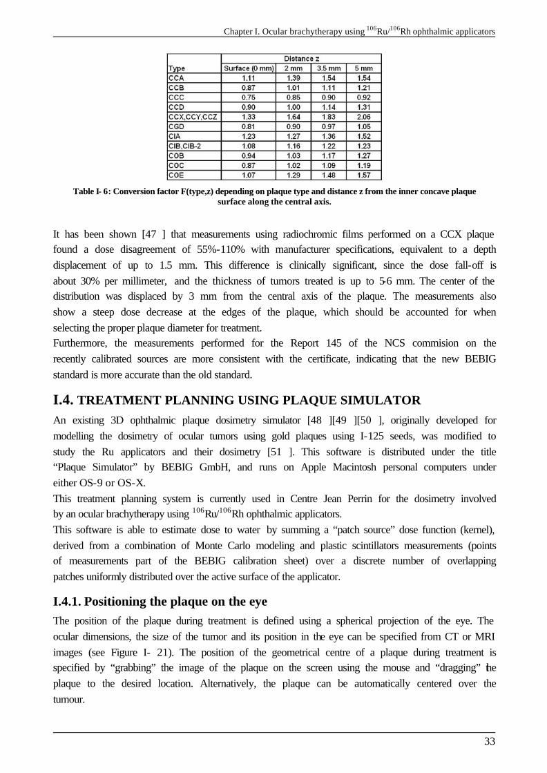
Chapter I. Ocular brachytherapy using 106Ru/106Rh ophthalmic applicators
33
Table I- 6: Conversion factor F(type,z) depending on plaque type and distance z from the inner concave plaque surface along the central axis.
It has been shown [47 ] that measurements using radiochromic films performed on a CCX plaque found a dose disagreement of 55%-110% with manufacturer specifications, equivalent to a depth displacement of up to 1.5 mm. This difference is clinically significant, since the dose fall-off is about 30% per millimeter, and the thickness of tumors treated is up to 5-6 mm. The center of the distribution was displaced by 3 mm from the central axis of the plaque. The measurements also show a steep dose decrease at the edges of the plaque, which should be accounted for when selecting the proper plaque diameter for treatment. Furthermore, the measurements performed for the Report 145 of the NCS commision on the recently calibrated sources are more consistent with the certificate, indicating that the new BEBIG standard is more accurate than the old standard.
I.4. TREATMENT PLANNING USING PLAQUE SIMULATOR An existing 3D ophthalmic plaque dosimetry simulator [48 ][49 ][50 ], originally developed for modelling the dosimetry of ocular tumors using gold plaques using I-125 seeds, was modified to study the Ru applicators and their dosimetry [51 ]. This software is distributed under the title “Plaque Simulator” by BEBIG GmbH, and runs on Apple Macintosh personal computers under either OS-9 or OS-X. This treatment planning system is currently used in Centre Jean Perrin for the dosimetry involved by an ocular brachytherapy using 106Ru/106Rh ophthalmic applicators. This software is able to estimate dose to water by summing a “patch source” dose function (kernel), derived from a combination of Monte Carlo modeling and plastic scintillators measurements (points of measurements part of the BEBIG calibration sheet) over a discrete number of overlapping patches uniformly distributed over the active surface of the applicator.
I.4.1. Positioning the plaque on the eye The position of the plaque during treatment is defined using a spherical projection of the eye. The ocular dimensions, the size of the tumor and its position in the eye can be specified from CT or MRI images (see Figure I- 21). The position of the geometrical centre of a plaque during treatment is specified by “grabbing” the image of the plaque on the screen using the mouse and “dragging” the plaque to the desired location. Alternatively, the plaque can be automatically centered over the tumour.
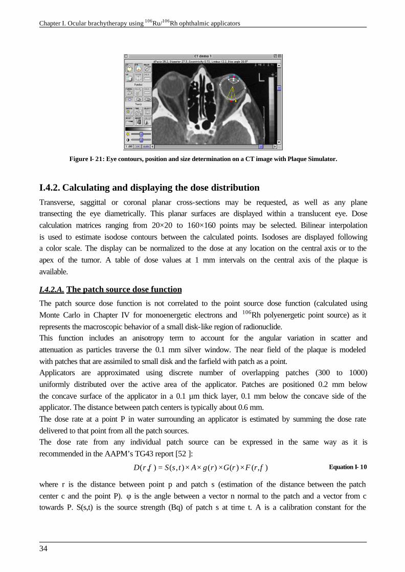
Chapter I. Ocular brachytherapy using 106Ru/106Rh ophthalmic applicators
34
Figure I- 21: Eye contours, position and size determination on a CT image with Plaque Simulator.
I.4.2. Calculating and displaying the dose distribution Transverse, saggittal or coronal planar cross-sections may be requested, as well as any plane transecting the eye diametrically. This planar surfaces are displayed within a translucent eye. Dose calculation matrices ranging from 20×20 to 160×160 points may be selected. Bilinear interpolation is used to estimate isodose contours between the calculated points. Isodoses are displayed following a color scale. The display can be normalized to the dose at any location on the central axis or to the apex of the tumor. A table of dose values at 1 mm intervals on the central axis of the plaque is available.
I.4.2.A. The patch source dose function
The patch source dose function is not correlated to the point source dose function (calculated using Monte Carlo in Chapter IV for monoenergetic electrons and 106Rh polyenergetic point source) as it represents the macroscopic behavior of a small disk-like region of radionuclide. This function includes an anisotropy term to account for the angular variation in scatter and attenuation as particles traverse the 0.1 mm silver window. The near field of the plaque is modeled with patches that are assimiled to small disk and the farfield with patch as a point. Applicators are approximated using discrete number of overlapping patches (300 to 1000) uniformly distributed over the active area of the applicator. Patches are positioned 0.2 mm below the concave surface of the applicator in a 0.1 µm thick layer, 0.1 mm below the concave side of the applicator. The distance between patch centers is typically about 0.6 mm. The dose rate at a point P in water surrounding an applicator is estimated by summing the dose rate delivered to that point from all the patch sources. The dose rate from any individual patch source can be expressed in the same way as it is recommended in the AAPM’s TG43 report [52 ]:
( , ) ( , ) ( ) ( ) ( , )D r S s t A g r G r F rφ φ= × × × × Equation I- 10
where r is the distance between point p and patch s (estimation of the distance between the patch center c and the point P). φ is the angle between a vector n normal to the patch and a vector from c towards P. S(s,t) is the source strength (Bq) of patch s at time t. A is a calibration constant for the
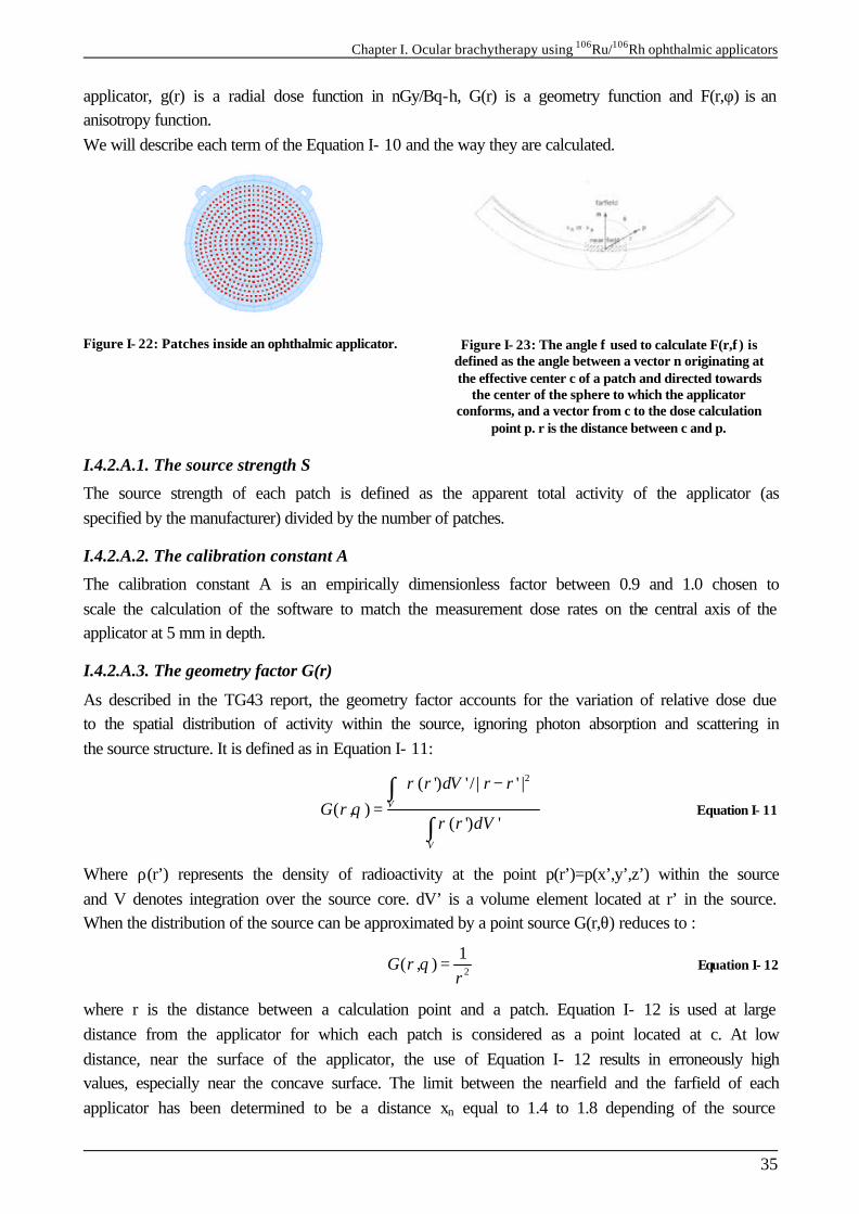
Chapter I. Ocular brachytherapy using 106Ru/106Rh ophthalmic applicators
35
applicator, g(r) is a radial dose function in nGy/Bq-h, G(r) is a geometry function and F(r,φ) is an anisotropy function. We will describe each term of the Equation I- 10 and the way they are calculated.
Figure I- 22: Patches inside an ophthalmic applicator.
Figure I- 23: The angle φ used to calculate F(r,φ) is defined as the angle between a vector n originating at the effective center c of a patch and directed towards
the center of the sphere to which the applicator conforms, and a vector from c to the dose calculation
point p. r is the distance between c and p.
I.4.2.A.1. The source strength S
The source strength of each patch is defined as the apparent total activity of the applicator (as specified by the manufacturer) divided by the number of patches.
I.4.2.A.2. The calibration constant A
The calibration constant A is an empirically dimensionless factor between 0.9 and 1.0 chosen to scale the calculation of the software to match the measurement dose rates on the central axis of the applicator at 5 mm in depth.
I.4.2.A.3. The geometry factor G(r)
As described in the TG43 report, the geometry factor accounts for the variation of relative dose due to the spatial distribution of activity within the source, ignoring photon absorption and scattering in the source structure. It is defined as in Equation I- 11: 2( ') ' / | ' |
( , )( ') '
V
V
r dV r rG r
r dV
ρθ
ρ
− =
∫
∫ Equation I- 11
Where ρ(r’) represents the density of radioactivity at the point p(r’)=p(x’,y’,z’) within the source and V denotes integration over the source core. dV’ is a volume element located at r’ in the source. When the distribution of the source can be approximated by a point source G(r,θ) reduces to :
2
1( , )G r
rθ = Equation I- 12
where r is the distance between a calculation point and a patch. Equation I- 12 is used at large distance from the applicator for which each patch is considered as a point located at c. At low distance, near the surface of the applicator, the use of Equation I- 12 results in erroneously high values, especially near the concave surface. The limit between the nearfield and the farfield of each applicator has been determined to be a distance xn equal to 1.4 to 1.8 depending of the source
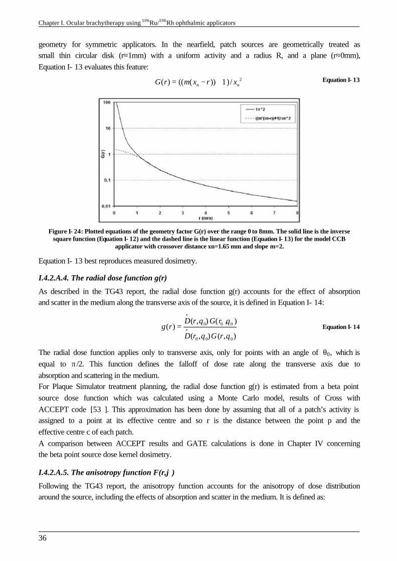
Chapter I. Ocular brachytherapy using 106Ru/106Rh ophthalmic applicators
36
geometry for symmetric applicators. In the nearfield, patch sources are geometrically treated as small thin circular disk (r≈1mm) with a uniform activity and a radius R, and a plane (r≈0mm), Equation I- 13 evaluates this feature: 2( ) (( ( )) 1)/n nG r m x r x= − + Equation I- 13
Figure I- 24: Plotted equations of the geometry factor G(r) over the range 0 to 8mm. The solid line is the inverse square function (Equation I- 12) and the dashed line is the linear function (Equation I- 13) for the model CCB
applicator with crossover distance xn=1.65 mm and slope m=2.
Equation I- 13 best reproduces measured dosimetry.
I.4.2.A.4. The radial dose function g(r)
As described in the TG43 report, the radial dose function g(r) accounts for the effect of absorption and scatter in the medium along the transverse axis of the source, it is defined in Equation I- 14:
0 0 0
0 0 0
( , ) ( , )( )
( , ) ( , )
D r G rg r
D r G r
θ θ
θ θ
•
•= Equation I- 14
The radial dose function applies only to transverse axis, only for points with an angle of θ0, which is equal to π/2. This function defines the falloff of dose rate along the transverse axis due to absorption and scattering in the medium. For Plaque Simulator treatment planning, the radial dose function g(r) is estimated from a beta point source dose function which was calculated using a Monte Carlo model, results of Cross with ACCEPT code [53 ]. This approximation has been done by assuming that all of a patch’s activity is assigned to a point at its effective centre and so r is the distance between the point p and the effective centre c of each patch. A comparison between ACCEPT results and GATE calculations is done in Chapter IV concerning the beta point source dose kernel dosimetry.
I.4.2.A.5. The anisotropy function F(r,ϕ)
Following the TG43 report, the anisotropy function accounts for the anisotropy of dose distribution around the source, including the effects of absorption and scatter in the medium. It is defined as:
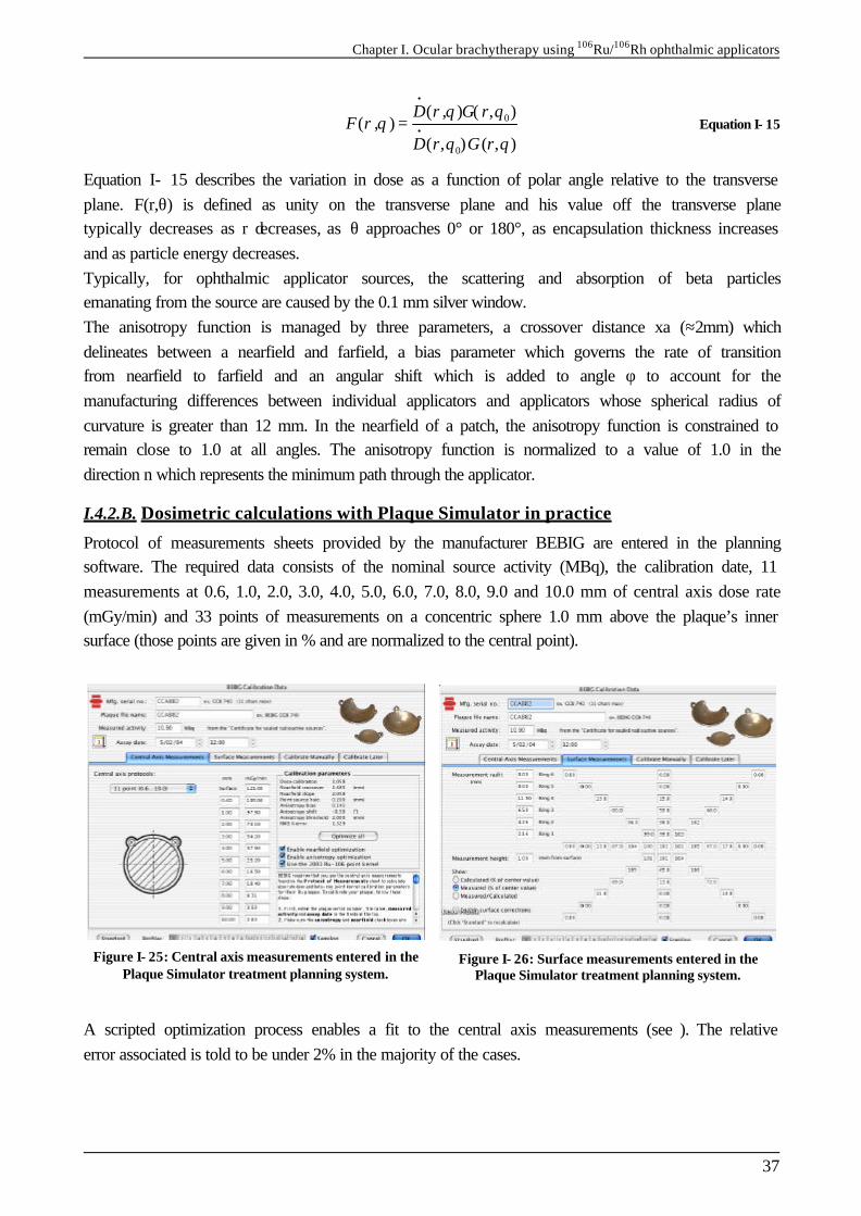
Chapter I. Ocular brachytherapy using 106Ru/106Rh ophthalmic applicators
37
0
0
( , ) ( , )( , )
( , ) ( , )
D r G rF r
D r G r
θ θθ
θ θ
•
•= Equation I- 15
Equation I- 15 describes the variation in dose as a function of polar angle relative to the transverse plane. F(r,θ) is defined as unity on the transverse plane and his value off the transverse plane typically decreases as r decreases, as θ approaches 0° or 180°, as encapsulation thickness increases and as particle energy decreases. Typically, for ophthalmic applicator sources, the scattering and absorption of beta particles emanating from the source are caused by the 0.1 mm silver window. The anisotropy function is managed by three parameters, a crossover distance xa (≈2mm) which delineates between a nearfield and farfield, a bias parameter which governs the rate of transition from nearfield to farfield and an angular shift which is added to angle φ to account for the manufacturing differences between individual applicators and applicators whose spherical radius of curvature is greater than 12 mm. In the nearfield of a patch, the anisotropy function is constrained to remain close to 1.0 at all angles. The anisotropy function is normalized to a value of 1.0 in the direction n which represents the minimum path through the applicator.
I.4.2.B. Dosimetric calculations with Plaque Simulator in practice
Protocol of measurements sheets provided by the manufacturer BEBIG are entered in the planning software. The required data consists of the nominal source activity (MBq), the calibration date, 11 measurements at 0.6, 1.0, 2.0, 3.0, 4.0, 5.0, 6.0, 7.0, 8.0, 9.0 and 10.0 mm of central axis dose rate (mGy/min) and 33 points of measurements on a concentric sphere 1.0 mm above the plaque’s inner surface (those points are given in % and are normalized to the central point).
Figure I- 25: Central axis measurements entered in the Plaque Simulator treatment planning system.
Figure I- 26: Surface measurements entered in the Plaque Simulator treatment planning system.
A scripted optimization process enables a fit to the central axis measurements (see ). The relative error associated is told to be under 2% in the majority of the cases.
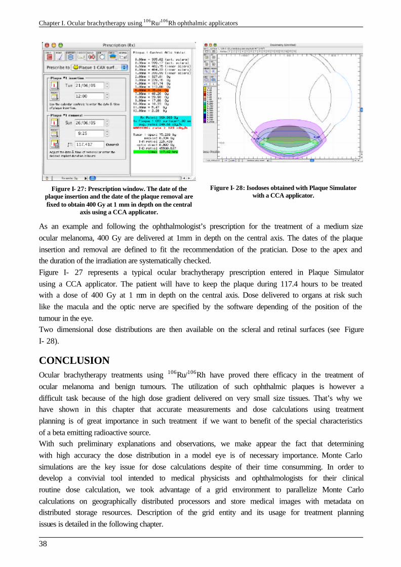
Chapter I. Ocular brachytherapy using 106Ru/106Rh ophthalmic applicators
38
Figure I- 27: Prescription window. The date of the plaque insertion and the date of the plaque removal are fixed to obtain 400 Gy at 1 mm in depth on the central
axis using a CCA applicator.
Figure I- 28: Isodoses obtained with Plaque Simulator with a CCA applicator.
As an example and following the ophthalmologist’s prescription for the treatment of a medium size ocular melanoma, 400 Gy are delivered at 1mm in depth on the central axis. The dates of the plaque insertion and removal are defined to fit the recommendation of the pratician. Dose to the apex and the duration of the irradiation are systematically checked. Figure I- 27 represents a typical ocular brachytherapy prescription entered in Plaque Simulator using a CCA applicator. The patient will have to keep the plaque during 117.4 hours to be treated with a dose of 400 Gy at 1 mm in depth on the central axis. Dose delivered to organs at risk such like the macula and the optic nerve are specified by the software depending of the position of the tumour in the eye. Two dimensional dose distributions are then available on the scleral and retinal surfaces (see Figure I- 28).
CONCLUSION Ocular brachytherapy treatments using 106Ru/106Rh have proved there efficacy in the treatment of ocular melanoma and benign tumours. The utilization of such ophthalmic plaques is however a difficult task because of the high dose gradient delivered on very small size tissues. That’s why we have shown in this chapter that accurate measurements and dose calculations using treatment planning is of great importance in such treatment if we want to benefit of the special characteristics of a beta emitting radioactive source. With such preliminary explanations and observations, we make appear the fact that determining with high accuracy the dose distribution in a model eye is of necessary importance. Monte Carlo simulations are the key issue for dose calculations despite of their time consumming. In order to develop a convivial tool intended to medical physicists and ophthalmologists for their clinical routine dose calculation, we took advantage of a grid environment to parallelize Monte Carlo calculations on geographically distributed processors and store medical images with metadata on distributed storage resources. Description of the grid entity and its usage for treatment planning issues is detailed in the following chapter.
Chapter I. Ocular brachytherapy using 106Ru/106Rh ophthalmic applicators
39
References [1 ] R.E. Tjho-Heslinga, J. Davelaar, H. M. Kemme, H. de Vroome, J.A. Oosterhuis, J.C. Bleeker,
J.W.H. Leer, “Results of ruthenium irradiation of uveal melanomas: the Dutch experience”, Radiotherapy and Oncology 53, pp 133-137, 1999.
[2 ] “Dosimetry of External Beta Rays for Radiation Protection”, ICRU report No. 56, 1997. [3 ] COMS (Collaborative Ocular Melanoma Study). http://www.jhu.edu/wctb/coms/ [4 ] Lommatzsch PK. “Treatment of choroidal melanoma with 106Ru/106Rh beta ray applicators”.
Surv. Ophtalmo.; 19(2): 85-100, 1974. [5 ] Lommatzsch PK. “Results after β-irradiation (106Ru/106Rh) of choroidal melanomas: 20 years’
experience. Br. J. Ophthalmol. ; 70:844-851, 1986. [6 ] Lommatzsch PK, Weise B., Ballin R., Ein Beitrag zur Optimierung der Bestrahlungszeit bei der
Behandlung des malignen Melanoms der Aderhaut mit β-Applikatoren (106Ru/106Rh). Klin. Monatsbl. Augenheilkd. 189:133-140, 1986.
[7 ] Lommatzsch PK, Kirsch IH. “106Ru/106Rh plaque radiotherapy for malignant melanomas of the choroid with follow-up results more than 5 years”. Doc. Ophthalmol. 68:225-238, 1988.
[8 ] Davelaar J., Schaling DF., Hennen LA., Broerse JJ., Dosimetry of ruthenium-106 eye applicators. Med. Phys. 19(3):691-694, 1992.
[9 ] Grange JD., Joshi G., Gérard JP., Jean-Louis B., Senténac I., Ayzac L. Bilan de dix années d’expériences de la béta-curiethérapie de contact par applicateur de ruthénium 106, pour mélanome de l’uvée. Revus de 207 cas et hommage à Lommatzsch. Ophtalmologie ; 9 :317-323, 1995.
[10 ] Kleineidam M., Guthoff R., Bentzen SM. Rates of local control, metas tasis, and overall survival in patients with posterior uveal melanomas treated with ruthenium-106 plaques. Radiother. Oncol.; 28:148-156, 1993.
[11 ] Seregard S., trampe EAF., Lax I., Kock E., Lundell G., Results following episcleral ruthenium plaque radiotherapy for posterior uveal melanoma. The Swedish experience. Acta. Ophthalmol. Scand.; 75: 11-16, 1997.
[12 ] Summanem P., Immonem I., Heikkonen J., Tommila P., Laatikainen L., Tarkkanen A. Survival of patients and metastatic and local recurrent tumour growth in malignant melanoma of the uvea after ruthenium plaque radiotherapy. Ophthal. Surg.; 25:82-90, 1993.
[13 ] Summanem P., Immonem I., Kivelä T., Tommila P., Heikkonen J., Tarkanen A. Visual outcome of eyes with malignant melanoma of the uvea after ruthenium plaque radiotherapy. Ophthal. Surg. Lasers; 26: 449-460, 1995.
[14 ] Summanem P., Immonem I., Kivelä T., Tommila P., Heikkonen J., Tarkanen A. Radiation related complications after ruthenium plaque radiotherapy of uveal melanoma. Br. J. Ophthalmol.; 80:732-739, 1996.
[15 ] Müller RP., Buss H., Pötter R., Kroll P., Haverkamp U. “Results of high dose 106-ruthenium irradiation of choroidal melanaomas.” Int. J. Radiat. Oncol. Biol. Phys. ; 12:1749-1755, 1986.
[16 ] Pötter R., Janssen K., Prott FJ., et al. Ruthenium-106 eye plaque brachytherapy in the conservative treatment of the uveal melanoma: evaluation of 175 patients treated with 150 Gy from 1981-1989. In: Wie gel T., Bornfeld N., Foerster MH., et al., editors. Radiotherapy of ocular disease. Front. Radiat. Ther. Oncol., 30., pp. 143-149, 1997.
[17 ] Polak BC, Wijngaarde R., Radiation retinopathy in patients with both diabetes mellitus and ophthalmic Graves’ disease. Orbit.; 14:71-74, 1995.
[18 ] Viebahn M., Barricks ME., Osterloh MD., Synergism between diabetic and radiation retinopathy. Br. J. Ophthalmol.; 75:629-632, 1991.
[19 ] Supe SJ, Mallikarjuna Rao S, Sawant SG. “Dosimetry of spherical Sr-90-Y-90 beta ray eye applicators.” Am J Roentgenol Radium Ther Nucl Med. 1975 Jan;123(1):36-41
[20 ] F. Bacin, S. Amara, J.L. Kemeny, R. Rozan, J.J. Bard, D. Donnarieix, « Etude comparative de l’irradiation béta (106Ru/106Rh) et de l’irradiation gamma (125I) sur l’œil de lapin », Ophthalmologica 1998 ; 212, pp429-438.
[21 ] S. Nag, J.M. Quivey, J.D. Earle, D. Followill, J. Fontanesi, P.T. Finger, “the American Brachytherapy Society recommendations for brachytherapy of uveal melanomas,” Int. J. Radiat. Oncol., Biol., Phys. 56, pp 544-555, 2003.
[22 ] P.T. Finger, “Tumor location affects the incidence of cataract and retinopathy after ophthalmic plaque radiation therapy,” Br. J. Ophthalmol. 84, pp 1068-1070, 2000.
Chapter I. Ocular brachytherapy using 106Ru/106Rh ophthalmic applicators
40
[23 ] J.S. Pruit, C.G. Soares, and M. Ehrlich, “Calibration of beta-particle radiation instrumentation and sources,”NBS Special publication 250-21, 1988.
[24 ] M. Piessens and N. Reynaert,”Verification of absolute dose rates for intravascular brachytherapy beta sources,”Phys.Med.Biol. 45: 2219-2231, 2000
[25 ] A. Niroomand-Rad, C.R. Blackwell, B.M. Coursey, K.P. Gall, J.M. Galvin, W.L. McLaughlin, A.S. Meigooni, R. Nath, J.E. Rodgers and C.G. Soares. “Radiochromic film dosimetry: recommendations of AAPM Radiation Therapy,” Committee Task Group 55. American Association of Physicists in Medicine Med.Phys. 25: 2093-2115, 1998.
[26 ] J.A. Sayeg and R.C. Gregory, “A new method for characterizing beta-ray ophthalmic applicator sources”, Med.Phys. 18: 453-461, 1991.
[27 ] C.G. Soares, “A method for the calibration of concave 90Sr+90Y ophthalmic applicators”, Phys.Med.Biol. 37: 1005-1007, 1992.
[28 ] C.G. Soares, D.G. Halpern and C.K. Wang, “Calibration and characterization of beta-particle sources for intravascular brachytherapy,” Med.Phys. 25: 339-346, 1998.
[29 ] C.G. Soares, S. Vynckier, H. Jarvinen, W.G. Cross, P. Sipila, D. Fluhs, B. Schaeken, F.A. Mourtada, G.A. Bass and T.T. Williams, “Dosimetry of beta-ray ophthalmic applicators: comparison of different measurement methods”, Med.Phys. 28: 1373-1384, 2001.
[30 ] C.S. Reft, F.T. Kuchnir, I. Rosenberg, and L.C. Myrianthopoulos, « Dosimetry of Sr-90 ophthalmic applicators », Med.Phys. 17: 641-646, 1990.
[31 ] D.R. Schaart, A.J. Bos, A.J. Winkelman and M.C. Clarijs, “The radial depth-dose distribution of a 188W/188Re beta line source measured with novel ultra-thin TLDs in a PMMA phantom: comparison with Monte Carlo simulations “, Phys.Med.Biol. 47: 3605-3627, 2002.
[32 ] L. Missotten, W. Dirven, A. Van der Schueren, A. Leys, G. De Meester and E. Van Limbergen, “Results of treatment of choroidal malignant melanoma with high-dose- rate strontium-90 brachytherapy. A retrospective study of 46 patients treated between 1983 and 1995”, Graefes Arch.Clin.Exp.Ophthalmol. 236: 164-173, 1998.
[33 ] W. Binder, A. Chiari and H. Aiginger, “Determination of the dose distribution of an ophthalmic 106Ru irradiator with TLDs and an eye phantom”, Rad.Prot.Dosim. 34: 275-278, 1990.
[34 ] D. Siddle and K. Langmack, “Calibration of strontium-90 eye applicator using a strontium external beam standard”, Phys.Med.Biol. 44: 1597-1608, 1999.
[35 ] B. Schaeken and P. Scalliet, “One year of experience with alanine dosimetry in radiotherapy”, Appl.Radiat.Isot. 47: 1177-1182, 1996.
[36 ] D. Flüs, M. Heintz, F. Indenkämpen, C. Wieczorek, H. Kolanski and U. Quast, “Direct reading measurement of absorbed dose with plastic scintillators,” Med.Phys. 23, pp 427-434 (1996).
[37 ] M. Heydarian, P.W. Hoban, W.A. Beckham, I.M. Borchardt and A.H. Beddoe,”Evaluation of a PTW diamond detector for electron beam measurements”, Phys.Med.Biol. 38: 1035-1042, 1993.
[38 ] S. Vatnitsky and H. Jarvinen, “Application of a natural diamond detector for the measurement of relative dose distributions in radiotherapy”, Phys.Med.Biol. 38: 173-184, 1993.
[39 ] G. Rikner and E. Grusell, “General specifications for silicon semiconductors for use in radiation dosimetry”, Phys.Med.Biol. 32: 1109-1117, 1987.
[40 ] I. Lax, “Dosimetry of 106Ru eye applicators with a p-type silicon detector”, Phys.Med.Biol. 36: 963-972, 1991.
[41 ] M.F. Chan, A.Y. Fung, Y.C. Hu, C.S. Chui, H. Amols, M. Zaider and D. Abramson, “The measurement of three dimensional dose distribution of a ruthenium- 106 ophthalmological applicator using magnetic resonance imaging of BANG polymer gels”, J.Appl.Clin.Med.Phys. 2: 85-89, 2001.
[42 ] M.J. Maryanski, G.S. Ibbott, P. Eastman, R.J. Schulz and J.C. Gore, “Radiation therapy dosimetry using magnetic resonance imaging of polymer gels”, Med.Phys. 23: 699-705, 1996.
[43 ] S.L. Meeks, F.J. Bova, M.J. Maryanski, L.A. Kendrick, M.K. Ranade, J.M. Buatti and W.A. Friedman, “Image registration of BANG gel dose maps for quantitative dosimetry verification”, Int.J.Radiat.Oncol.Biol.Phys. 43: 1135-1141, 1999.
[44 ] R.P. Kollaard, W.J.F. Dries, H.J. van Kleffens, A.H.L. Aalbers, J. van der Marel, J.P.A. Marijnissen, M. Piessens, D.R. Schaart, H. de Vroome, “Report 14 of the Netherlands Commission on Radiation Dosimetry”, “Quality control of sealed beta sources in brachytherapy, Recommendations on detectors, measurement procedures and quality control of beta sources”, August 2004.
[45 ] ICRU (International Commission on Radiation Units and Measurements), “Dosimetry of beta rays and low-energy photons for brachytherapy with sealed sources”, ICRU Report 72,
Chapter I. Ocular brachytherapy using 106Ru/106Rh ophthalmic applicators
41
rays and low-energy photons for brachytherapy with sealed sources”, ICRU Report 72, preliminary version, August 2001.
[46 ] IAEA (International Atomic Energy Agency), “Calibration of photon and beta ray sources used in brachytherapy”, IAEA-TECDOC-1274, Vienna, 2002. http://www-naweb.iaea.org/nahu/external/e3/publications.asp
[47 ] S. Trichter et al., “Treatment Planning for Ru-106 Eye Plaques”, Pitfalls and Remedies, Poster at RSNA 2002 - 88th Scientific Assembly and Annual Meeting.
[48 ] M. Astrahan, G. Luxton, G. Jozsef, T.D. Kampp, P. Liggett and M.D. Sapozink, “An interactive treatment planning system for ophthalmic plaque radiotherapy”, Int. J. Radiat. Oncol., Biol., Phys. 18, pp 679-687, 1990.
[49 ] M. Astrahan, G. Luxton, G. Joszef, P.Liggett and Z. Petrovich, “Optimization of I-125 ophthalmic plaque brachytherapy, “ Med. Phys. 17, pp 1053-1057, 1990.
[50 ] M. D. C. Evans, M.A. Astrahan and R. Bate, “Tumor localization using fundus view photography for episcleral plaque therapy”, Med. Phys. 17, pp 1053-1057, 1990.
[51 ] M.A. Astrahan, “A patch source model for treatment planning of ruthenium ophthalmic applicators”, Med. Phys. 30 (6), pp 1219-1228, June 2003.
[52 ] M.J. Rivard, B.M. Coursey, L.A. DeWerd, W.F. Hanson, M.S. Huq, G.S. Ibbott, M.G. Mitch, R. Nath, J.F. Williamson, “Update of AAPM Task Group No. 43 Report: A revised AAPM protocol for brachytherapy dose calculations”, Med. Phys. 31 (3), pp 633-673, March 2004.
[53 ] W.G. Cross, J. Hokkanen, H. Järvinen, F. Mourtada, P. Sipilä, C.G. Soares, S. Vynckier, “Calculation of beta-ray dose distributions from ophthalmic applicators and comparison with measurements in a model eye”, Med. Phys. 28 (7), pp 1385-1396, July 2001.

Chapter I. Ocular brachytherapy using 106Ru/106Rh ophthalmic applicators
42
Chapter II.Grid technologies and health related applications
43
Chapter II.
Grid technologies and health related applications INTRODUCTION Computers are still used much less extensively than they could be and it’s obvious to say that the average computing environment remains inadequate for computationally sophisticated purposes. To answer computational, large and distributed storage, and sharing datasets needs, the grid technologies appeared. From a technology point of view, radiotherapy is a highly complex procedure, involving a variety of computational operations for data gathering, processing and control. The modularity of the treatment process and the need of large data sets from different sources and nature (physics, mathematics, bio-statistics, biology, and medicine) make it a privileged candidate for healthgrid applications. In an enlarged Europe sharing data, expertise and computational resources will be a significant factor for a successful cost containment and improved access to a high overall quality of care in radiotherapy. It is an ideal tool for harmonising the cancer treatment as well as providing a common base for research collaboration. Adding the fact that Monte Carlo simulations are more and more integrated to the elaboration of accurate treatment planning for specific applications, such like ocular brachytherapy using 106Ru/106Rh ophthalmic applicators, the grid could be a great alternative to reduce the computation time involved by such calculations. Based on the HealthGrid White paper published in 2005 [50 ], the first part of this chapter is dedicated to grid for health related applications. Issues concerning eHealth are described first; the healthGrid association federating a large community of researchers implied in grid improvements for health applications is detailed next, to finish with a description of what it has been envisaged to use grids for radiotherapy planning. After an overview of the grid computing projects that appeared in Europe over the last four years, the European DataGrid Project (EDG) intended to develop middleware of a grid infrastructure is described in a next part. A subparts is intended to achievements realized over the period of the project to build the grid infrastructure.
Chapter II.Grid technologies and health related applications
44
The third part describes the nature of the production grid infrastructure EGEE by highlighting the computing efficacy involved by using the grid. A discussion on the specific needs for the management of medical imaging and metadata on the grid with the first achievements performed in that domain is then done.
II.1. GRID FOR HEALTH RELATED APPLICATIONS
II.1.1. The challenges for eHealth eHealth is becoming the 3rd industrial pillar of healthcare after phramaceutical and medical imaging device industries. The eHealth retailers predict a benefit of more than $22B (US) for the year 2004. Most of the challenges encounter in eHealth applications must be overcome in the next year and can benefit of the grid technologies. § First of all, the Health related data require long-term and large storage to store patient
records comprising images, bio-signals, plain text, videos, photographs or other forms of digital data.
§ The medical data (images, programs, etc…) must be linked with databases with medical information. Federated databases should then emerge between clinical centres, laboratories and hospitals.
§ Medical information can require high bandwidth connections to meet minimum delay requirements for the pratician. That implies that technologies must converge to a high-bandwidth communication networks between healthcare centres.
§ Obtain the same degree of electronic management of patient data over healthcare centres. The Electronic Patient Record (EPR) enabling a coherent access to and the management of the complete patient information should achieve an easier access to data. The standardization of the data recording should also be reached in a near future to facilitate their management and utilization by each medical actors.
§ Last but not least, the security is the most important issue. The access to the information must be performed only by authorized and authenticated persons and data must be encrypted to guarantee its confidentiality and integrity. Personal data are identified to be any piece of information in which its owner can be identified, either directly or in combination with information that is available or otherwise located. Furthermore, electronic archiving of personal data is strictly regulated by the European and national laws.
Grids applied to health related applications must provide services or middleware components that deal with the specific problems arising in the processing of biomedical data. Although the ultimate goal for eHealth in Europe would be the creation of a single health grid, i.e. a grid comprising all eHealth resources, naturally including security and authorization features to handle subsidiarity of independent nodes of the healthgrid, the development path will mostly likely include a set of specific health grids with perhaps rudimentary inter-grid interaction/interoperational capabilities. The future evolution of grid technologies addresses most precisely problems that are very appropriate for healthcare. Health grid applications are oriented to both the individualized healthcare and the epidemiology analysis. Individualized healthcare is improved by the efficient and
Chapter II.Grid technologies and health related applications
45
secure combination of immediate availability of personal clinical information and widespread availability of advanced services for diagnostic and therapy. Epidemiology healthgrids combine the information from a wide population to extract the knowledge that can lead to the discovery of new correlations between symptoms, diseases, genetic features or any other clinical data. Facing to the growing of interest into providing grid tools for health related applications in the last Grid projects, the Healthgrid entity has born. In the following we will refer to the “Healthgrid white paper” [42 ] and to related work in the EDG [50 ] and EGEE project to describe what are the prospects and requirements to turn a grid to a health related grid. In the next part, we will focus especially on the computational models in medical imaging and therapy to be deployed in a grid environment. The Healthgrid white paper and all the information related to grid computing dedicated to health applications can be found on the healthgrid web site http://www.healthgrid.org.
II.1.2. The HealthGrid association Over the last four years, a community of researchers working on Grid and High Performance Computing technologies started discussing the barriers and opportunities that grid technologies must face and exploit for the development of health-related applications. This interest lead to the first Healthgrid conference, held in Lyon, France, on January 16th-17th, 2003, with the focus of creating increased awareness about the possibilities and advantages linked to the deployment of grid technologies in health, ultimately targeting the creation of a European/international grid infrastructure for health. The topics of this conference converged with the position of the eHealth division of the European Commission, whose mandate from the Lisbon Meeting was “To develop an intelligent environment that enables ubiquitous management of citizens’ health status, and to assist health professionals in coping with some major challenges, risk management and the integration into clinical practice of advances in health knowledge.” In this context "Health" involves not only clinical procedures but covers the whole range of information from molecular level (genetic and proteomic information) over cells and tissues, to the individual and finally the population level (social healthcare). Grid technology offers the opportunity to create a common working backbone for all different members of this large "health family" and will hopefully lead to an increased awareness and interoperability among disciplines. The first HealthGrid conference led to the creation of the Healthgrid association, a non-profit research association legally incorporated in France but formed from the broad community of European researchers and institutions sharing expertise in health grids. After the second Healthgrid conference, held in Clermont-Ferrand on January 29th-30th, 2004, the need for a “white paper” on the current status and prospective of health grids was raised. Over fifty experts from different areas of grid technologies, eHealth applications and the medical world were invited to contribute to the preparation of this document. The association named Healthgrid [43 ] and governed by the French law of July 1, 1901 and the decree of August 16, 1901 has been founded in April 2003. The goal of the association is: § to contribute to the structuring of the European Research Area for health, by, for example,
favouring the use of grid technologies;
Chapter II.Grid technologies and health related applications
46
§ to offer active support and guidelines for the extension of the association's members contribution to society;
§ to supply information and other services relevant to the members of the association; § to encourage co-operation between the members of the association, notably in the creation
of effective networks of collaboration; § create partnerships of benefit to both higher education and scientific research in the field of
the health in its broadest sense, both within Europe and in the rest of the world. The HealthGrid is the coordinator of the SHARE project, part of the IST call 4, FP6 2004, intended to “Supporting and structuring HealthGrid Activities & Research in Europe: developing a roadmap”. The project will define a comprehensive and detailed European R&D roadmap, covering both technology and policy aspects, to guide and promote beneficial EU-wide uptake of HealthGrid technologies and applications into health research, and into health care service provision.
II.1.3. Health grids: a grid scenario for radiotherapy planning (from the HealthGrid white paper [50 ])
II.1.3.A. Processing simulations in a grid environment
Research communities in biocomputing or biomodelling and simulation have a strong need for resources that can be provided through the grid. Compliance with medical information standards is necessary for accessing large databases. There are many consolidated and emerging standards that must be taken into account. Complex and multimedia information such as images, signals, videos, etc. is clearly a target for grid and is more sensitive to data formats. Finally, flexibility is needed for the control of VOs at a large level. The management of resources should be more precise and dynamic, depending on many criteria such as urgency, users’ authorization or other administrative policies. Biocomputing medical applications are one of the family of healthgrid applications. The maturity of genetics and biomedical technologies brings them closer to medicine, and grand-challenge computing problems of biocomputing are currently being migrated to grid. Biomedical modelling and simulation is another important area for grid applications. For this second application, we will highlight in the following part the issues that have to reach to enable therapy planning in routine using a grid infrastructure.
II.1.3.B. Issues for therapy planning
Many human body models have been developed for therapy planning. Examples of numerical simulation used by health practitioners include radio-surgery/radio-therapy planning, electromagnetic source localisation (an inverse procedure to identify areas of disorder within the brain based on external EEG/MEG measurements), reconstructive maxillofacial surgery, etc. Today, most developments are in the transition between research use and clinical use. Grid can be used to provide access to appropriate computational services and deliver these to medical users. Healthgrid would need large scale deployment studies to allow the evaluation of a wide range of requirements, including local deployment aspects and practical experience with production grid use. The major challenges will be to ensure that services can be delivered into the user’s workplace in an
Chapter II.Grid technologies and health related applications
47
appropriate, ergonomic manner and that security, policy and legal constraints related to the use of patient data are fulfilled.
II.1.3.B.1. A grid scenario for radiotherapy planning and treatment
Radiotherapy and Genes
Presently patients are treated with standardised radiation doses. Gene profiling may enable an individualised adjustment of the dose so as to achieve tumour control in patients with a low radiosensitivity and avoid severe side effects in patients with above average sensitivity to radiation. In a first step a grid structure should allow research groups, each focusing on different molecular mechanisms, to access data in the distributed infrastructure for comparison studies. In a next step users should be able to submit the results of predictive tests for analysis to a shared software and expert platform for radiosensitivity grading. A similar approach can be followed for other aspects clinical decision making such as the assessment a tumour’s capacity for metastatic spread. For rapidly metastasising tumours, systemic (chemotherapy) treatment needs to be associated to the locally delivered radiotherapy. New tests now under development, predicting on the basis of gene profiling which tumours are most likely to metastasise, can make 60% of the chemotherapy currently administered e.g. for breast cancer, redundant. However, it takes a highly specialised team to interpret the results of these tests correctly. Grid-supported consultation of libraries of gene profiles or, alternatively, tele-consulting services offer also in these case excellent perspectives.
Medical images for radiotherapy treatments
Tissue electron density provided by CT scanning is still needed to calculate the dose delivered by photon and electron beams. To define the planning target volume (PTV) and organs-at-risk (OAR), new imaging modalities based on MR-imaging, MR-spectroscopy and PET are complementary to CT scans and become a requirement for high-precision high-dose radiotherapy. In contrast to CT scanning, the latter imaging modalities are available only in reference centres for reasons of cost and expertise. To secure access for all patients to optimal imaging for radiotherapy planning, the coordinating centre could perform a grid-mediated selection of an imaging centre, and the resulting complementary image acquisitions could be sent back through the grid. To reproduce the patient positioning and perform the complementary imaging in treatment-relevant conditions, the patient-individual immobilisation devices could be physically sent to the imaging centre. Alternatively, a retrospective registration grid service could be used to realign all the images in the relevant coordinate system. Many tools have been developed for computer-aided definition of PTV and OAR including anatomical atlases that can be warped to the patient-individual anatomy. A grid could make such tools and their upgrades in due time available to all groups involved in PTV and OAR definition. Nodes on the grid that provide expert help for patient-related problems in defining PTV and OAR are needed.
Monte Carlo simulations for dose calculation
Accuracy of Monte Carlo (MC) dose computation is excellent, provided that the computing power is sufficient to allow for enough runs to reduce the statistical noise. The grid is a natural alternative
Chapter II.Grid technologies and health related applications
48
to costly parallel computers. In this way, MC dose computations could become standard for radiotherapy quality assurance (QA), planning, and plan optimisation years before individual departments could afford a local investment that is capable to support MC. Requirements needed for such deployment include the existence of a service level agreement between the departments and the grid providers by which the grid level of performances in terms of security, stability and response time is guaranteed. Each delivery centre manages the commissioning of its own treatment units and incorporates both mechanical-physical and dosimetric parameters, including uncertainty flags, into an identity card that is accessible through the grid. This identity card will allow treatment-planning providers and computation services to establish, refine or fit their computational model of the linear accelerator. The identity card also contains the reference data so that periodical quality assurance (QA) procedures could make sure that the machine performs accordingly. One might expect that the cooperation through the grid between QA providers and delivery centres will streamline the QA procedures and harmonise the identity cards over the different accelerator types. The quality assurance of the treatment can also benefit from the grid, even if it is patient specific: once a treatment plan has been designed, some locations are selected to measure the dose level in a physical phantom that replaces the patient during the first treatment session. In parallel, the coordinating centre consults the grid for an independent dose computation service to compute the dose in the same set of points in the phantom. The comparison of the measured dose to the computed fractional dose is performed automatically at the delivery centre and will be submitted to the coordinating centre. In case of violation of tolerances, the treatment plan will be recomputed in patient and phantom by a second dose computation service in the grid. Alternatively, the coordinating centre may consult the grid for a virtual treatment at another delivery centre.
Conclusion
Those previous requirements describe what should be enable in a near future to compute and manage radiotherapy treatments in a grid environment. The work to perform in order to achieve all those described aspects is still long but, in this thesis, we began to reflect and develop tools for ocular brachytherapy treatments using Monte Carlo. In the following parts of this chapter, we enumerate and discuss what are the grid functionnalities enabled at this date and argue about the grid computing efficacy and medical data management, the two main aspects involved in radiotherapy treatments nowadays.
II.2. GRID COMPUTING IN EUROPE The computational grid can be associated by analogy to an electric power grid. Computation is equivalent to electricity and transmission and distribution technologies could be combined to grid capabilities. We talk about an infrastructure because computational grid is concerned by large-scale pooling resources but also by people, connections, data, etc. Different levels can be found for grid users: grid developers in charge of designing and implementing the basic services, tool developers who create the compilers, libraries that implement the programming models and services used by application developers, application developers who construct grid enabled applications and components, end users who will not write programs, but will use grid-enabled applications that make use of grid resources and services and finally system administrators who manage the infrastructure on which computational grids operate. All these features require a significant
Chapter II.Grid technologies and health related applications
49
hardware infrastructure for interconnections and software infrastructure to monitor and control this entity. Furthermore, grids have to develop a middleware layer capable of adressing application requirements coming from different scientific communities such as High Energy Physics, Earth Observation and Biomedical applications for which the requirements are surely the most complex and the most challenging for middleware developers.
II.2.1. European and national grid projects Since 2000, the European Commission has been financing Grid research under the fifth research framework program (FP5) with more than 50 million Euros, as part of the European Union's Information Society Technologies (IST) research [1 ]. In FP5, the focus was mainly on technology development and application pilots. The main projects in FP5 were the European Data Grid [2 ], GridLab [3 ], EUROGrid [4 ], CROSSGrid [5 ] and DATATAG [6 ]. In FP6, beginning in 2002 and extending to 2006, the European Union is funding Grid research with more than 140 million Euros, following a technology push/application pull approach (i.e., developing the underlying technologies and Grid-enabling "real-world" applications). The crucial enabling infrastructure for the current research Grid projects is GEANT [7 ], the world's most powerful research network which links more than 3,000 research institutions across Europe. In the first phase, the European Union has launched several significant Grid initiatives which help structure the Grid infrastructures in Europe and build upon the already established GEANT infrastructure, most notably EGEE (Enabling Grids for E-Science) [8 ] [9 ] and DEISA (operating a distributed/Grid terascale supercomputing facility across Europe) [10 ] . In 2004, the EU has approved another 12 FP6 Grid projects, among them four major projects with a focus on Grid infrastructure technologies that will create a critical mass of expertise and resources from across Europe: § CoreGrid is a "network of excellence" addressing longer term Grid research, creating the
foundations for the next-generation Grids toward 2010 and beyond. The project brings together existing Grid research communities by creating virtual centers of excellence.
§ NextGrid is an integrated project focusing on the underlying technologies of the Next Generation Grid, aiming to deliver a new Grid architecture by the end of the decade. The work addresses security and business models, taking into account requirements from sectors such as finance and media.
§ Akogrimo is developing mobile Grid architectures and services. Building on Europe's strengths in mobile communications, the project will demonstrate a vision of dynamic virtual organizations in pilot applications in e-health and e-learning.
§ SIMDAT is an integrated project developing generic Grid technologies for industry in the areas of data integration, collaboration and knowledge discovery. The focus is on the use of Grids to solve complex problems in important sectors such as aerospace, automotive, pharmacology and meteorology.
In addition, seven smaller projects (K-WF Grid, UniGrids, HPC4U, inteliGrid, OntoGrid, DataMining Grid and Provenance) focus on specific targets, such as knowledge extraction, workflows, data mining, collaboration, trust and security.

Chapter II.Grid technologies and health related applications
50
With the UK e-Science projects (investments of more than 118 million pounds) a vast variety of Grid research, middleware, applications and industry projects born such as: DAME (Distributed Aircraft Maintenance Environment); GridCast (Grid for television/radio broadcasting); RiskGrid (for risk assessment calculations in financial services); GRIA (Grid Resources for Industrial Applications); MyGrid (a Grid portal for Bioinformatics research); and OGSA-DAI (Grid Resources for data access and integration). At GGF12 [11 ] in Berlin in the spring of 2004, the German Minister for Education and Research announced a five-year, 100-million-Euro e-Science program. Germany started as early as 1996 with the development of UNICORE [12 ], a uniform access infrastructure connecting German supercomputer and research centers. Germany is now investing a larger portion of the 100 million Euros in the development of D-Grid, a countrywide general Grid research infrastructure and Grid services initiative, along with several community Grids for community-specific middleware and Grid-enabled applications that focus on specific research areas. Other national and regional Grid initiatives are: the French Grid5000 project, the e-Toile projects the Instruire project (for the Auvergne region); the Italian GRID.IT; the DutchGrid and the 40-million-Euro Dutch VL-e project to develop a virtual laboratory for e-Science in the Netherlands; the Grid-Ireland MarineGrid, CosmoGrid and WebCom-G projects; the NorduGrid with its Advanced Resource Connector (ARC) Grid middleware used by SweGrid, Estonian Grid, M-Grid in Finland, the Danish Production Grid and others; the Austrian Grid Initiative with focus on infrastructure, middleware and applications, and its ASKALON Grid application development and computing environment; Poland's PROGRESS Grid, combining resources in Krakow, Poznan, Lodz and other cities via its powerful PIONEER network; and the SEE-Grid for South Eastern European Grid-enabled e-Infrastructure Development, with partners from Greece, Bulgaria, Romania, Turkey, Hungary and Yugoslavia. Europe now has a long-term, coordinated and shared Grid R&D vision, mission, strategy, roadmap and funding, driven by the European Commission's IST Framework Programmes 5, 6 and 7 (the latter will start in 2007).
II.2.2. The European Datagrid Project (EDG) The European Datagrid IST project [2 ] has came to completion at the end of March 2004 after a final review by the european commission. The main objective of the project was to develop a middleware layer capable of addressing application requirements coming from three different communities: High Energy Physics, Earth Observation, and Biomedical applications. Early in the project, two communities were identified inside the biomedical applications working group: the bioinformatics and the medical imaging communities in which GATE applications was implied. The DataGrid project was organized in working groups (or Work packages) dedicated to the middleware (5 WPs), the testbed infrastructure (2 WPs), the application communities (3 WPs) and the project management (2 WPs).
II.2.2.A. Organization
Grid Work scheduling (WP1): The objectives of this WP were:

Chapter II.Grid technologies and health related applications
51
§ The optimisation of the program executing location in function of the availability of data, computing power and network.
§ The allocation of resources necessary to execute programs. § The development of a common interface to access resource management systems available
on the grid. § The definition of priorities and rights to access resources.
Data Management (WP2): The goal of this work package was to specify, develop, integrate and test tools and middleware infrastructure to coherently manage and share petabyte-scale information volumes in high-throughput production quality grid environments. The main purposes of this WP were to: § allow a secure access to massive amounts of data in a universal global name space, § move and replicate data at high speed from one geographical site to another, § manage synchronisation of remote replicas. § Develop a generic interface to heterogeneous mass storage management systems to enable
seamless and efficient integration of distributed resources. Information and monitoring services (WP3): The aim of this workpackage was to specify, develop, integrate and test tools and infrastructure to enable end-user and administrator access to status and error information in a Grid environment and to provide an environment in which application monitoring can be carried out. Fabric management (WP4): The objective of this WP was to develop tools enabling the installation and the automated management of the middleware components on computing resources (clusters). Mass Storage management (WP5): This WP was in charge of identify the different storage modalities used by the different scientific communities to develop a management file system. The Integration testbed and support WP (WP6) was in charge of testing the grid middleware. As a fully functional Data Grid depend critically on the nature and quality of the underlying network. Performance (bandwidth, latency), security, quality of service, and reliability are all key factors. Data Grid use the European (GEANT) and national research network infrastructures to provide a large set of network services between the computational and data resources that form the Data Grid testbeds thanks to the WP7 (Network services). This WP is in charge of four tasks: § Planning for provisioning of infrastructure for testbed operation § Network and Transport Services § Network and Grid traffic monitoring § Grid Security
The last three WPs group the scientific applications: Particle physics (LHC experiments) was represented by the WP8, the Earth Observation by the WP9 and biomedical applications, grouping medical imaging, bioinformatics and radiotherapy planification treatments using Monte Carlo was represented by WP10. GATE Monte Carlo applications have been designed to be one of the demonstration application presented to the European Comission during the final review of the EDG project in February 2004.
Chapter II.Grid technologies and health related applications
52
II.2.2.B. Achievements and lessons learned
The EDG project grouped more than 500 users under 12 organisations with more than 600 persons trained to use the Grid infrastructure. One million of lines of code have been produced under 7 major middleware releases. Six High Energy physics experiments, ten biomedical applications and five Earth Observation institutes joined the project as applications. At the end of the project the application testbed was constituted of 20 sites representing 1000 CPUs and 6 Mass storage systems. The early distributed testbed was based on Globus 1 [13 ]; after having established the Certification Authorities (see description in II.3.1.c.1), the development of the higher grid middleware started with the workload management, the data management, the Information services and the Fabric management (see description in II.3.1.b.2). The first testbed was deployed in the middle of 2001 on five sites and the first application evaluation started in december 2001 with a first High Energy Physics job run. In September 2001, the CERN launched the LCG project [15 ]. After the first review successfully passed on March 1st 2002, the evaluation by end users revealed the need to focus on the stability of the middleware rather than on new functionality. An open source license was established in June 2002 and the tutorial program started in July of the same year during GGF5. The second testbed was delivered at the end of 2002 (release 1.4.x) and allowed first production tests for applications. The 2nd annual review was successfully passed in February 2003 and the third testbed (release 2.x) enabling a better scalability and reliability was released at the end of August 2003, the release 2.1 was produced at the end of November 2003. Many components of the EDG 2.0 were deployed in the LCG-1 services (during summer 2003) and the EDG 2.1 largely influenced the LCG-2 components at the beginning of 2004. The final DataGrid review was presented in February 2004 and successfully passed, GATE applications was one of the demonstration presented to the European Comission as part of the biomedical applications. The main assets the DataGrid project developed are: § A large scale testbed continuously available throughout the project duration § The elaboration of 21 Certification Authority infrastructure § An innovative middleware with all the components described here after in part II.3.1.b.2. § A software released under OSI approved open source license that facilitates wide-spread
usage and encourages feedback. § Application groups that are an integral part of the project contributing to all aspects of work.
Lessons learned are numerous, one of them is that application groups need to be involved in all phases of the decisions. The middlewere prototypes should have been available for application testing early. The cross activities between the WPs need to be coordinated. Furthermore, it has been highlighted that different testbeds should have been distributed: one to test bleeding edge software and an other one for the production infrastructure. Security services need to be an integrated part from the very beginning of the project to fit requirements of users, in particularly for the biomedical community. The EGEE project, intended to develop a production testbed has benefited of the gained experience in the EDG project and also of the developments performed in the LCG-2 middleware. The EGEE production testbed is described in the next part with a discussion concerning the current grid computing efficacy.

Chapter II.Grid technologies and health related applications
53
II.3. THE EGEE (Enabling Grid for E-sciencE) PROJECT
II.3.1. Presentation The EGEE Grid will be built on the EU Research Network GÉANT [7 ] and exploit Grid expertise generated by many EU, national and international Grid projects to date. Funded by the European Commission, the EGEE project community has been divided into 12 partner federations, consisting of over 70 contractors and over 30 unfunded participants covering a wide-range of both scientific and industrial applications. The work being carried out in the project is organised into 11 activities. Two pilot application domains have been selected to guide the implementation and certify the performance and functionality of the evolving infrastructure. One is the Large Hadron Collider Computing Grid supporting physics experiments and the other is Biomedical, where several communities are facing equally daunting challenges to cope with the flood of bioinformatics and healthcare data. With funding of over 30 million euros from the European Commission, the project is one of the largest of its kind. EGEE is a two-year project conceived as part of a four-year programme, where the results of the first two years will provide the basis for assessing subsequent objectives and funding needs.
II.3.1.A.1. EGEE activities
EGEE is organized into eleven activities which come under three main areas: § Networking Activities (NA) which are the management and coordination of all the
commmunication aspects of the project § Specific Service Activities (SA) are the support, operation and management of the Grid as
well as the provision of network resources § Research Activities (JRA) concentrate on Grid research and development
EGEE Networking activities (NA): § Networking Activity 1 (NA1) is the overall management of the project. § Networking Activity 2 (NA2) is Information Dissemination and Outreach and includes tasks
such as running the external website, organising conferences and managing the distribution of publications.
§ Networking Activity 3 (NA3) is User Training and Induction and includes tasks such as organising on-site training and producing training and course material.
§ Networking Activity 4 (NA4) is Application Identification and Support and includes tasks such as supporting pilot applications and identifying new users. GATE applications are part of the NA4.
§ Networking Activity 5 (NA5) is Policy and International Cooperation and includes tasks such as liaising with parties interested in the EGEE project on an international level.
EGEE Specific Service Activities (SA): § Specific Service Activity 1 (SA1) is European Grid Support, Operation and Management
and includes tasks such as grid monitoring and control and resource and user support.
Chapter II.Grid technologies and health related applications
54
§ Specific Service Activity 2 (SA2) is Network Resource Provision and includes tasks such as policies and service level agreements.
EGEE Joint Research activities (JRA): § Joint Research Activity 1 (JRA1) is Middleware Re-engineering and Integration, it includes
tasks such as re-engineering existing middleware, integrating middleware, testing and validation.
§ Joint Research Activity 2 (JRA2) is Quality Assurance, it includes tasks such as ensuring that processes, products and operation services conform to project requirements, standards and procedures.
§ Joint Research Activity 3 (JRA3) is Security, it includes tasks such as developing security frameworks and policies and designing security mechanisms.
§ Joint Research Activity 4 (JRA4) is Network Service Development, it includes tasks such as developing interfaces to the network and advance reservations of network connectivity in terms of bandwidth, duration and quality of service.
Biomed applications are part of the NA4. In the following section we will describe the goals of the NA4 and the biomed applications implied in it.
II.3.1.A.2. The objectives of the NA4
§ Support the deployment and running of many different applications from various fields. At this date, twelve applications are part of the Biomed Applications. Each of them are part of sub-groups corresponding to different categories of applications:
ü "Pilot" applications will be used to test EGEE middleware and to evaluate performances. GATE (Geant4 Applications for Tomographic Emission), CDSS (Clinical Decision Support System) and GPS@ (Grid Genomic Web Portal) are part of this category.
ü "Internal" applications will come from within the project in the sense that they involve EGEE partners in collaboration with institutes external to the project. SiMRI 3D (Magnetic Resonance Image simulator), gPTM 3D (interactive radiological image visualization and processing tool), xmipp_Mlrefine (Macromolecular 3D structure analysis), GridGRAMM (Molecular Docking web), GROCK ( Mass screenings of molecular interactions web), WISDOM (grid-enabled docking platform for in sillico drug discovery) and Xmipp_assign_multiple_CTFs (Micrographia CTF calculation) are part of this category.
ü "External" applications which come from collaborations external to the project and will need support for deployment on EGEE. SPLATCHE (genome evolution modeling) and the Mammogrid project whom aim is to develop a European-wide database of mammograms that will be used to investigate a set of important healthcare applications as well as the potential of this Grid to support effective co-working between healthcare professionals throughout the EU.

Chapter II.Grid technologies and health related applications
55
§ Provide necessary feedback to Middleware and Operations, this particularly the case for pilot applications.
§ Produce deliverables: All along the 2 years of the duration of the project, report (deliverables) have to be presented. Concerning NA4, for which GATE and biomedical applications in general are part, six deliverables must be produced: during the third month of the project, DNA4.1 (Definition of Common Application Interface and Planning Document) elaborates the milestones of the NA4 applications; during the sixth month of the project, then follows DNA4.2 (Target Application Sector Strategy document) and for the ninth, fifteenth and twenty fourth month of the project, DNA4.3.1-3 concerning EGEE Application Migration Progress report are produced.
II.3.1.B. The EGEE infrastructure
II.3.1.B.1. The Grid middleware
The LCG middleware
As the EDG middleware isn’t upgraded any longer since the end of the project in February 2004 (EDG 2.1.2). The first middleware that will be used on the "production" infrastructure is the LHC Computing grid [14 ] [15 ] [16 ] [17 ] LCG-2. LCG-2 has been derived from the EDG middleware but offers a few more facilities and has better documentation. The Large Hadron Collider (LHC), which is being constructed at the European Organization for Particle Physics (CERN), will be the world’s largest and most powerful particle accelerator. The accelerator will start operation in 2007, and the experiments that will use it will generate large amounts of data. The processing of this data will require enormous computational and storage resources. The job of the LHC Computing Grid Project [15 ] –LCG– is to prepare the computing infrastructure for the simulation, processing and analysis of LHC data for all four of the LHC collaborations: ALICE, ATLAS, CMS and LHCB. The LCG-1 middleware (first version) was based on Globus 2.2.4 and benefited of the work done in EDG WP1 concerning the Resource Broker [18 ] and the Workload Management System (WMS) [19 ] implementation, the EDG WP2 Replica Management tools and the Glue 1.1 [24 ] information schema. The LCG modifications focus on the job managers to avoid shared filesystems problems, MDS and BDII-LDAP, Globus gatekeeper enhancements and bug fixes to EDG and Globus/VDT [25 ]. The LCG-2 release was available at the beginning of 2004, LCG-2 expands the services of LCG-1, with enough resources and functionality for the 2004 Computing Data Challenge. The LCG-2 middleware provides the experience on operating and managing a global grid service and benefits of a development program driven by data challenge experience: the data handling, the strenghtening of the infrastructure and the users and entity management (VO). The EGEE infrastructure was entirely based in April 2004 on the LCG-2 middleware to migrate in the middle of 2005 to a new one called gLite [26 ].
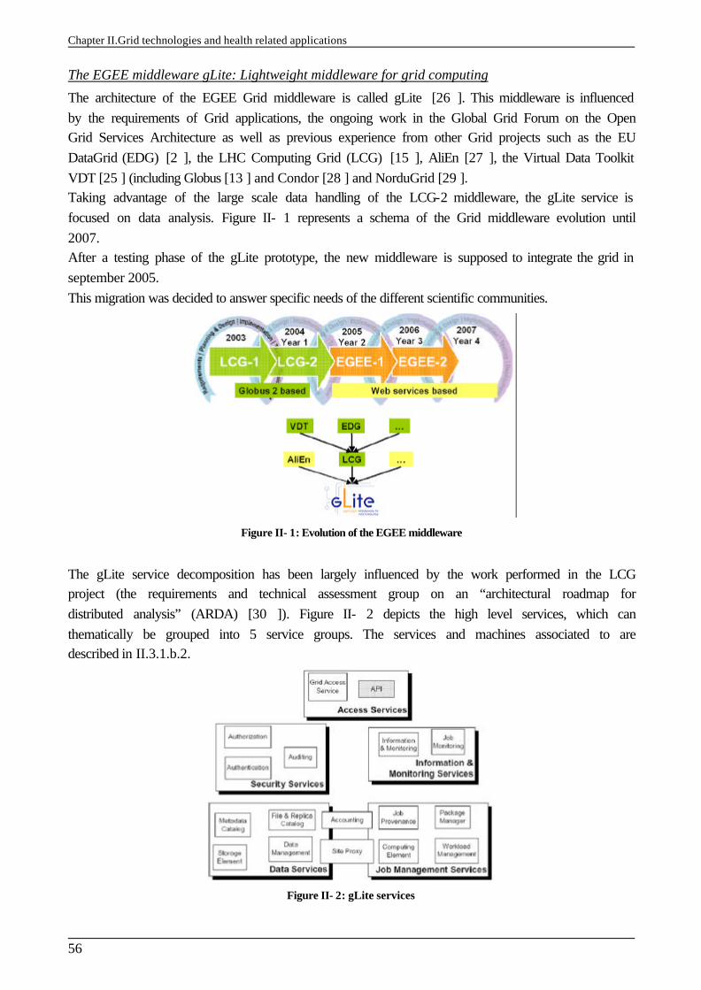
Chapter II.Grid technologies and health related applications
56
The EGEE middleware gLite: Lightweight middleware for grid computing
The architecture of the EGEE Grid middleware is called gLite [26 ]. This middleware is influenced by the requirements of Grid applications, the ongoing work in the Global Grid Forum on the Open Grid Services Architecture as well as previous experience from other Grid projects such as the EU DataGrid (EDG) [2 ], the LHC Computing Grid (LCG) [15 ], AliEn [27 ], the Virtual Data Toolkit VDT [25 ] (including Globus [13 ] and Condor [28 ] and NorduGrid [29 ]. Taking advantage of the large scale data handling of the LCG-2 middleware, the gLite service is focused on data analysis. Figure II- 1 represents a schema of the Grid middleware evolution until 2007. After a testing phase of the gLite prototype, the new middleware is supposed to integrate the grid in september 2005. This migration was decided to answer specific needs of the different scientific communities.
Figure II- 1: Evolution of the EGEE middleware
The gLite service decomposition has been largely influenced by the work performed in the LCG project (the requirements and technical assessment group on an “architectural roadmap for distributed analysis” (ARDA) [30 ]). Figure II- 2 depicts the high level services, which can thematically be grouped into 5 service groups. The services and machines associated to are described in II.3.1.b.2.
Figure II- 2: gLite services

Chapter II.Grid technologies and health related applications
57
All the services should be deployed and used independently, allowing their exploitation in different contexts. As the gLite grid services follow a Service Oriented Architecture, the interoperability among Grid services will be facilitated.
II.3.1.B.2. Machines and services part of the EGEE infrastructure
The User Interface
The User Interface (UI) is the gateway to the EGEE grid services. This machine hosts personal user account and user’s certificate. From the UI, a user can be authenticated and authorized to use the EGEE Grid resources. This is the component that allows users to access the functionalities offered by the Information, Workload and Data management services. It provides the Commands Line Interface (CLI) to perform the Grid operations.
The Computing Element and Storage Element
A Computing Element (CE) is defined as a Grid batch queue and it is identified by a pair <hostname>:<port>/<batch queue name>. This is currently used to define different queues for jobs of different lengths. Examples of CE names in Clermont-Ferrand site: clrce01.in2p3.fr:2119/jobmanager-lcgpbs-long clrce01.in2p3.fr:2119/jobmanager-lcgpbs-short A Computing Element is built usually on a homogeneous farm of computing nodes called Worker Nodes (WN) and a node acting as a Grid Gate (GG) or front-end to the rest of the Grid. The GG runs a Globus gatekeeper, the Globus GRAM (Globus Resource Allocation Manager) [Ref], the master server of a Local Resource Management System (LRMS), together with the a local Logging and Bookkeeping server (see ). The types of LRMS supported are the Portable batch System (PBS), the Load Sharing Facility (LSF) and Condor. While all WNs need only outbound connectivity, the Gate node must be accessible from outside the site. The GG is responsible for accepting jobs and dispatching them for execution to the WNs. On the WNs, all commands and Application Programming Interface (API) for performing actions on Grid resources and Grid data are available. Each EGEE site runs at least one CE and a farm of WNs behind it. A Storage Element (SE) provides uniform access and services to large storage spaces. The Storage Element may control large disk arrays, mass storage systems (MSS) and the like. Almost EGEE sites provide one or more SEs. A site can include at least a classic SE, which has a GSIFTP server [31 ].The GSIFTP protocol offers basically the functionality of FTP, i.e. used for the transfers of files, but enhanced to use GSI security. It is responsible for secure, fast and efficient file transfer to/from the Storage Element. Thus, the main file access protocol in the Grid is GSIFTP [31 ], which is used for the transfering of files, and which will be always supported by any Grid storage resource. However, for the remote access (and not only copy) of files stored in the SEs, the protocol to be used is the Remote File Input/Output protocol (RFIO) [32 ]. The resources described up to now constitute the compute and storage power of the LCG-2 Grid.
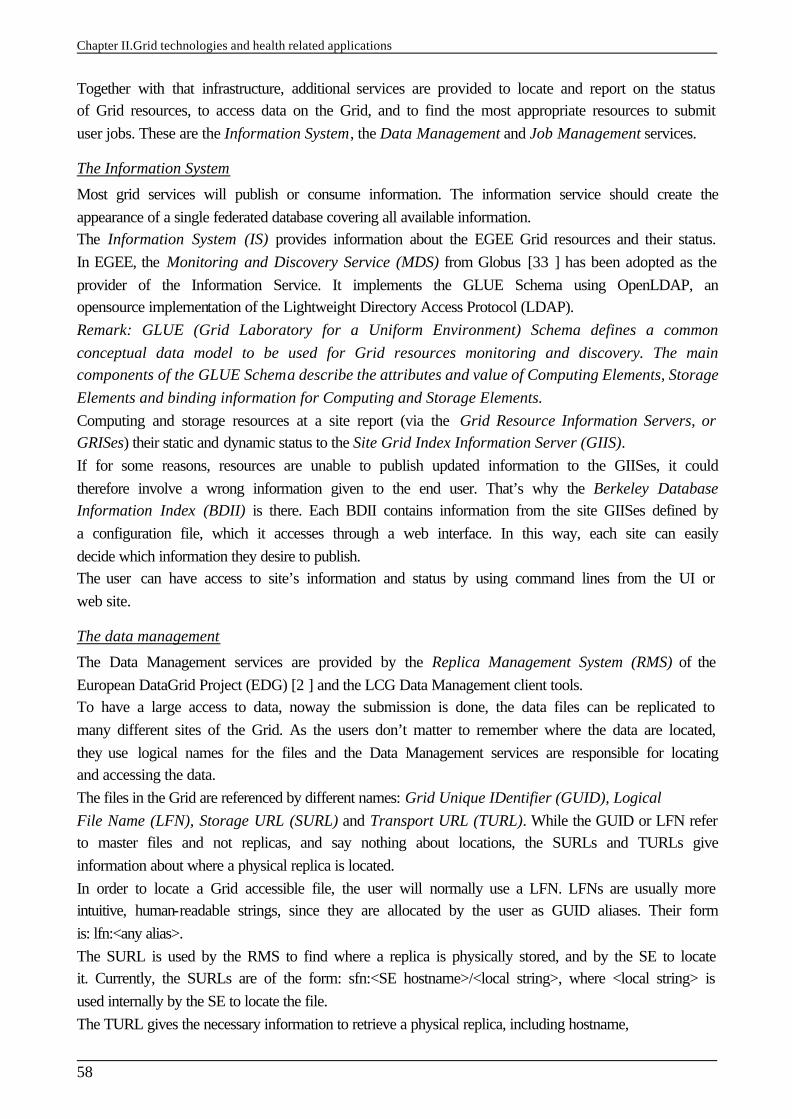
Chapter II.Grid technologies and health related applications
58
Together with that infrastructure, additional services are provided to locate and report on the status of Grid resources, to access data on the Grid, and to find the most appropriate resources to submit user jobs. These are the Information System, the Data Management and Job Management services.
The Information System
Most grid services will publish or consume information. The information service should create the appearance of a single federated database covering all available information. The Information System (IS) provides information about the EGEE Grid resources and their status. In EGEE, the Monitoring and Discovery Service (MDS) from Globus [33 ] has been adopted as the provider of the Information Service. It implements the GLUE Schema using OpenLDAP, an opensource implementation of the Lightweight Directory Access Protocol (LDAP). Remark: GLUE (Grid Laboratory for a Uniform Environment) Schema defines a common conceptual data model to be used for Grid resources monitoring and discovery. The main components of the GLUE Schema describe the attributes and value of Computing Elements, Storage Elements and binding information for Computing and Storage Elements. Computing and storage resources at a site report (via the Grid Resource Information Servers, or GRISes) their static and dynamic status to the Site Grid Index Information Server (GIIS). If for some reasons, resources are unable to publish updated information to the GIISes, it could therefore involve a wrong information given to the end user. That’s why the Berkeley Database Information Index (BDII) is there. Each BDII contains information from the site GIISes defined by a configuration file, which it accesses through a web interface. In this way, each site can easily decide which information they desire to publish. The user can have access to site’s information and status by using command lines from the UI or web site.
The data management
The Data Management services are provided by the Replica Management System (RMS) of the European DataGrid Project (EDG) [2 ] and the LCG Data Management client tools. To have a large access to data, noway the submission is done, the data files can be replicated to many different sites of the Grid. As the users don’t matter to remember where the data are located, they use logical names for the files and the Data Management services are responsible for locating and accessing the data. The files in the Grid are referenced by different names: Grid Unique IDentifier (GUID), Logical File Name (LFN), Storage URL (SURL) and Transport URL (TURL). While the GUID or LFN refer to master files and not replicas, and say nothing about locations, the SURLs and TURLs give information about where a physical replica is located. In order to locate a Grid accessible file, the user will normally use a LFN. LFNs are usually more intuitive, human-readable strings, since they are allocated by the user as GUID aliases. Their form is: lfn:<any alias>. The SURL is used by the RMS to find where a replica is physically stored, and by the SE to locate it. Currently, the SURLs are of the form: sfn:<SE hostname>/<local string>, where <local string> is used internally by the SE to locate the file. The TURL gives the necessary information to retrieve a physical replica, including hostname,
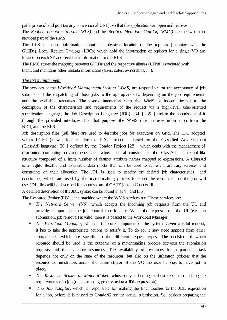
Chapter II.Grid technologies and health related applications
59
path, protocol and port (as any conventional URL); so that the application can open and retrieve it. The Replica Location Service (RLS) and the Replica Metadata Catalog (RMC) are the two main services part of the RMS. The RLS maintains information about the physical location of the replicas (mapping with the GUIDs). Local Replica Catalogs (LRCs) which hold the information of replicas for a single VO are located on each SE and feed back information to the RLS. The RMC stores the mapping between GUIDs and the respective aliases (LFNs) associated with them, and maintains other metada information (sizes, dates, ownerships. . . ).
The job management
The services of the Workload Management System (WMS) are responsible for the acceptance of job submits and the dispatching of those jobs to the appropiate CE, depending on the job requirements and the available resources. The user’s interaction with the WMS is indeed limited to the description of the characteristics and requirements of the request via a high-level, user-oriented specification language, the Job Description Language (JDL) [34 ] [35 ] and to the submission of it through the provided interfaces. For that purpose, the WMS must retrieve information from the BDII, and the RLS. Job description files (.jdl files) are used to describe jobs for execution on Grid. The JDL adopted within EGEE (it was identical for the EDG project) is based on the Classified Advertisement (ClassAd) language [36 ] defined by the Condor Project [28 ], which deals with the management of distributed computing environments, and whose central construct is the ClassAd, a record-like structure composed of a finite number of distinct attribute names mapped to expressions. A ClassAd is a highly flexible and extensible data model that can be used to represent arbitrary services and constraints on their allocation. The JDL is used to specify the desired job characteristics and constraints, which are used by the match-making process to select the resources that the job will use. JDL files will be described for submissions of GATE jobs in Chapter III. A detailed description of the JDL syntax can be found in [34 ] and [35 ]. The Resource Broker (RB) is the machine where the WMS services run. These services are: § The Network Server (NS), which accepts the incoming job requests from the UI, and
provides support for the job control functionality. When the request from the UI (e.g. job submission, job removal) is valid, then it is passed to the Workload Manager.
§ The Workload Manager, which is the core component of the system. Given a valid request, it has to take the appropriate actions to satisfy it. To do so, it may need support from other components, which are specific to the different request types. The decision of which resource should be used is the outcome of a matchmaking process between the submission requests and the available resources. The availability of resources for a particular task depends not only on the state of the resources, but also on the utilisation policies that the resource administrators and/or the administrator of the VO the user belongs to have put in place.
§ The Resource Broker or Match-Maker, whose duty is finding the best resource matching the requirements of a job (match-making process using a JDL expression).
§ The Job Adapter, which is responsible for making the final touches to the JDL expression for a job, before it is passed to CondorC for the actual submission. So, besides preparing the

Chapter II.Grid technologies and health related applications
60
CondorC submission file, this module is also responsible for creating the job wrapper script that creates the appropriate execution environment in the CE worker node (this includes the transfer of the input and of the output sandboxes). Then the job is passed to the Job control Service.
§ CondorC is the module responsible for performing the actual job management operations (job submission, job removal, etc.), issued on request of the Workload Manager.
§ Job Control Service (JCS), which finally performs the actual job management operations (job submission, removal. . . )
The Logging and Bookkeeping service (LB) is usually run on the RB machine. The LB logs all job management Grid events, which can then be retrieved by users or system administrators for monitoring or troubleshooting. All WMS components described before interact with the LB for logging information about the jobs they are handling and for querying information about them when needed. Moreover during the matchmaking phase the Resource Broker interacts with the Data Management Catalogs through the StorageIndex interface to resolve the locations of existing file names specified in the JDL Inputdata list, so that the submitted job would run on worker node, close to the used files. The WMS service also interacts with VOMS (see II.3.1.c.2) indirectly as it reads information about VO [38 ], groups and capabilities from the user’s proxy credentials issued by VOMS to enforce user authentication and authorization. The MyProxy service is contacted by the Proxy Renewal component of the WMS to renew automatically the credentials associated to long lived jobs. Last but not least the WMS interacts with the CEs for submitting jobs (this goes through CondorC) and for receiving synchronous/asynchronous notifications about resource status and characteristics. There could be configurations in which the WMS also interacts with the BDII to collect information about the whole resource pool available for a given VO.
II.3.1.B.3. A typical job flow in EGEE
Figure II- 3 illustrates the process that is followed by a job submitted to the Grid. The steps are defined as follow:
1) The user logs to the UI machine and creates a proxy certificate that authenticates him in every secure interaction, and has a limited lifetime. The user submits the job from the UI to the WMS, where the job will be executed on a computing node. The user can specify in the job description file one or more files to be copied from the UI to the RB node; this set of files is called Input Sandbox. The event is logged in the LB and the status of the job is SUBMITTED.
2) The WMS, and in particular the Match-Maker component, looks for the best available CE to
execute the job. To do so, the Match-Maker interrogates the BDII to query the status of computational and storage resources and the RLS to find location of data. The event is logged in the LB and the status of the job is WAITING.
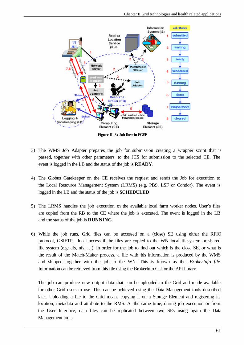
Chapter II.Grid technologies and health related applications
61
Figure II- 3: Job flow in EGEE
3) The WMS Job Adapter prepares the job for submission creating a wrapper script that is
passed, together with other parameters, to the JCS for submission to the selected CE. The event is logged in the LB and the status of the job is READY.
4) The Globus Gatekeeper on the CE receives the request and sends the Job for execution to
the Local Resource Management System (LRMS) (e.g. PBS, LSF or Condor). The event is logged in the LB and the status of the job is SCHEDULED.
5) The LRMS handles the job execution on the available local farm worker nodes. User’s files
are copied from the RB to the CE where the job is executed. The event is logged in the LB and the status of the job is RUNNING.
6) While the job runs, Grid files can be accessed on a (close) SE using either the RFIO
protocol, GSIFTP, local access if the files are copied to the WN local filesystem or shared file system (e.g: afs, nfs, …). In order for the job to find out which is the close SE, or what is the result of the Match-Maker process, a file with this information is produced by the WMS and shipped together with the job to the WN. This is known as the .BrokerInfo file. Information can be retrieved from this file using the BrokerInfo CLI or the API library.
The job can produce new output data that can be uploaded to the Grid and made available for other Grid users to use. This can be achieved using the Data Management tools described later. Uploading a file to the Grid means copying it on a Storage Element and registering its location, metadata and attribute to the RMS. At the same time, during job execution or from the User Interface, data files can be replicated between two SEs using again the Data Management tools.
Chapter II.Grid technologies and health related applications
62
If the job reaches the end without errors, the output (not large data files, but just small output files specified by the user in the so called Output Sandbox) is transferred back to the RB node. The event is logged in the LB and the status of the job is DONE.
7) At this point, the user can retrieve the output of his/her job from the UI using the WMS CLI or API. The event is logged in the LB and the status of the job is CLEARED.
Queries of the job status are addressed to the LB database from the UI machine. Also, from the UI it is possible to query the BDII for a status of the resources. If the site where the job is being run falls down, the job will be automatically resent to another CE that is analogue to the previous one, and following the same requirements the user asked for. In the case that this previous submissions are disabled (the user has the possibility to re-submit his jobs as he wants), the job will be marked as aborted. Users can get information about what happened by simply questioning the LB service.
II.3.1.C. Requirements for a user to access the grid
II.3.1.C.1. Obtaining a certificate
The first requirement the user must fulfil is to be in possession of a valid X.509 certificate issued by a recognized Certification Authority (CA). The role of a CA is to guarantee that a user is who he claims to be and is entitled to own his/her certificate. In general CAs are organized geographically and sometimes by research institute. Each CA follows the European Policy for Management Authority for Grid Authentication (EU Grid PMA) [39 ]. It is a body to establish requirements and best practices for grid identity providers to enable a common trust domain applicable to authentication of end-entities in inter-organisational access to distributed resourceshas its own procedure to release certificates.
II.3.1.C.2. Be part of a Virtual Organization (VO)
The second requirement for a Grid user is to belong to a Virtual Organization (VO). A VO is an entity, which corresponds typically to a particular organization or group of people in the real world. The membership of a VO grants specific privileges to the user. For example, a user belonging to the ATLAS VO will be able to read the ATLAS files or to exploit resources reserved to the ATLAS collaboration. Remark: This last specification is not suitable for the BIOMED VO because of confidentiality problems between each application and between users of each application. This is one of the special requirement of the BIOMED VO for the EGEE middleware gLite. Each medical data must be anonym and the access to it should be with privileges. This point is discussed in the sub-section concerning VOMS. It is not possible to access the Grid without being member of any VO. Every user is required to select his/her VO when registering and the supplied information is forwarded to the VO administration and resource prividers for validation before the registration process is completed.
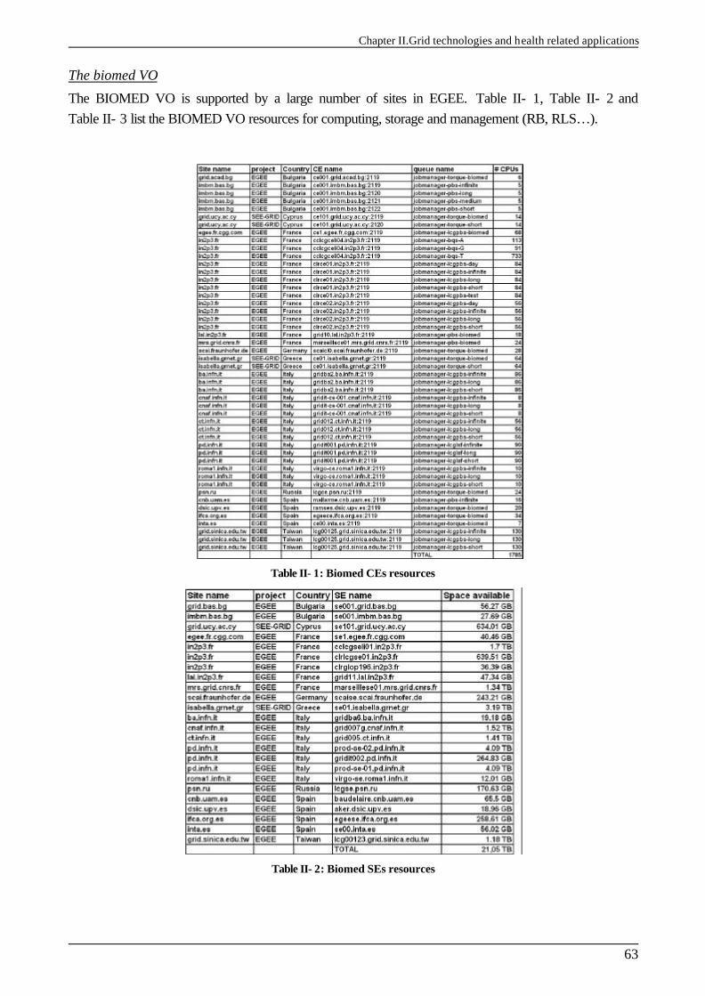
Chapter II.Grid technologies and health related applications
63
The biomed VO
The BIOMED VO is supported by a large number of sites in EGEE. Table II- 1, Table II- 2 and Table II- 3 list the BIOMED VO resources for computing, storage and management (RB, RLS…).
Table II- 1: Biomed CEs resources
Table II- 2: Biomed SEs resources
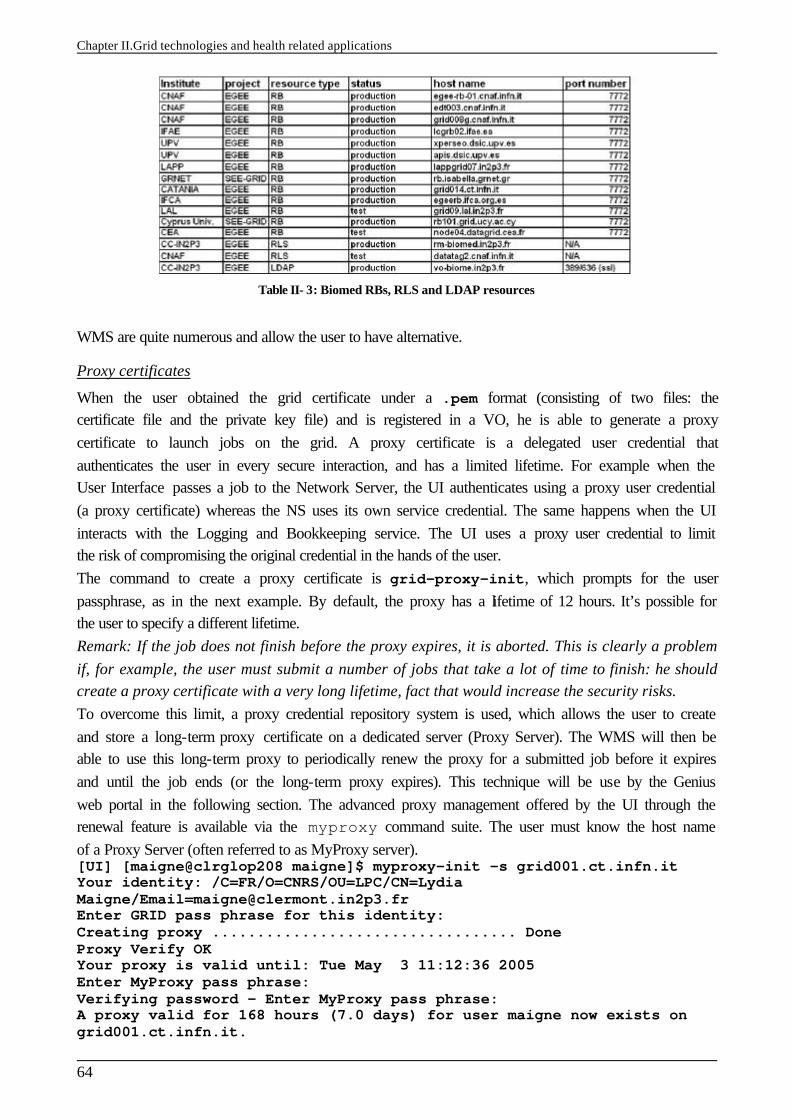
Chapter II.Grid technologies and health related applications
64
Table II- 3: Biomed RBs, RLS and LDAP resources
WMS are quite numerous and allow the user to have alternative.
Proxy certificates
When the user obtained the grid certificate under a .pem format (consisting of two files: the certificate file and the private key file) and is registered in a VO, he is able to generate a proxy certificate to launch jobs on the grid. A proxy certificate is a delegated user credential that authenticates the user in every secure interaction, and has a limited lifetime. For example when the User Interface passes a job to the Network Server, the UI authenticates using a proxy user credential (a proxy certificate) whereas the NS uses its own service credential. The same happens when the UI interacts with the Logging and Bookkeeping service. The UI uses a proxy user credential to limit the risk of compromising the original credential in the hands of the user. The command to create a proxy certificate is grid-proxy-init, which prompts for the user passphrase, as in the next example. By default, the proxy has a lifetime of 12 hours. It’s possible for the user to specify a different lifetime. Remark: If the job does not finish before the proxy expires, it is aborted. This is clearly a problem if, for example, the user must submit a number of jobs that take a lot of time to finish: he should create a proxy certificate with a very long lifetime, fact that would increase the security risks. To overcome this limit, a proxy credential repository system is used, which allows the user to create and store a long-term proxy certificate on a dedicated server (Proxy Server). The WMS will then be able to use this long-term proxy to periodically renew the proxy for a submitted job before it expires and until the job ends (or the long-term proxy expires). This technique will be use by the Genius web portal in the following section. The advanced proxy management offered by the UI through the renewal feature is available via the myproxy command suite. The user must know the host name of a Proxy Server (often referred to as MyProxy server). [UI] [maigne@clrglop208 maigne]$ myproxy-init –s grid001.ct.infn.it Your identity: /C=FR/O=CNRS/OU=LPC/CN=Lydia Maigne/[email protected] Enter GRID pass phrase for this identity: Creating proxy .................................. Done Proxy Verify OK Your proxy is valid until: Tue May 3 11:12:36 2005 Enter MyProxy pass phrase: Verifying password - Enter MyProxy pass phrase: A proxy valid for 168 hours (7.0 days) for user maigne now exists on grid001.ct.infn.it.
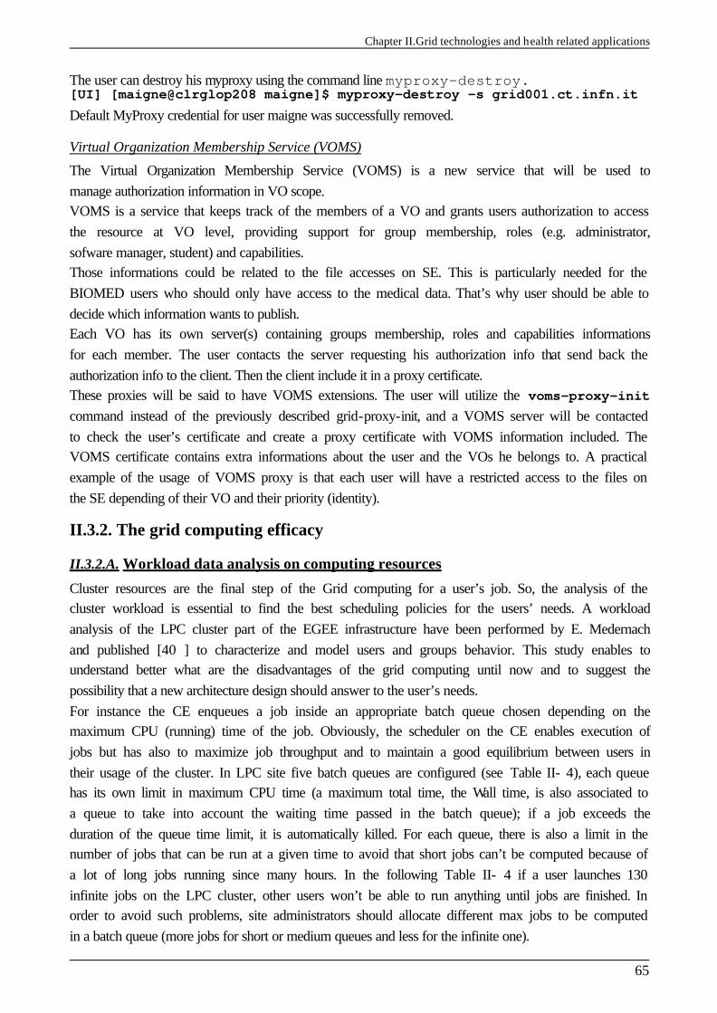
Chapter II.Grid technologies and health related applications
65
The user can destroy his myproxy using the command line myproxy-destroy. [UI] [maigne@clrglop208 maigne]$ myproxy-destroy -s grid001.ct.infn.it Default MyProxy credential for user maigne was successfully removed.
Virtual Organization Membership Service (VOMS)
The Virtual Organization Membership Service (VOMS) is a new service that will be used to manage authorization information in VO scope. VOMS is a service that keeps track of the members of a VO and grants users authorization to access the resource at VO level, providing support for group membership, roles (e.g. administrator, sofware manager, student) and capabilities. Those informations could be related to the file accesses on SE. This is particularly needed for the BIOMED users who should only have access to the medical data. That’s why user should be able to decide which information wants to publish. Each VO has its own server(s) containing groups membership, roles and capabilities informations for each member. The user contacts the server requesting his authorization info that send back the authorization info to the client. Then the client include it in a proxy certificate. These proxies will be said to have VOMS extensions. The user will utilize the voms-proxy-init command instead of the previously described grid-proxy-init, and a VOMS server will be contacted to check the user’s certificate and create a proxy certificate with VOMS information included. The VOMS certificate contains extra informations about the user and the VOs he belongs to. A practical example of the usage of VOMS proxy is that each user will have a restricted access to the files on the SE depending of their VO and their priority (identity).
II.3.2. The grid computing efficacy
II.3.2.A. Workload data analysis on computing resources
Cluster resources are the final step of the Grid computing for a user’s job. So, the analysis of the cluster workload is essential to find the best scheduling policies for the users’ needs. A workload analysis of the LPC cluster part of the EGEE infrastructure have been performed by E. Medernach and published [40 ] to characterize and model users and groups behavior. This study enables to understand better what are the disadvantages of the grid computing until now and to suggest the possibility that a new architecture design should answer to the user’s needs. For instance the CE enqueues a job inside an appropriate batch queue chosen depending on the maximum CPU (running) time of the job. Obviously, the scheduler on the CE enables execution of jobs but has also to maximize job throughput and to maintain a good equilibrium between users in their usage of the cluster. In LPC site five batch queues are configured (see Table II- 4), each queue has its own limit in maximum CPU time (a maximum total time, the Wall time, is also associated to a queue to take into account the waiting time passed in the batch queue); if a job exceeds the duration of the queue time limit, it is automatically killed. For each queue, there is also a limit in the number of jobs that can be run at a given time to avoid that short jobs can’t be computed because of a lot of long jobs running since many hours. In the following Table II- 4 if a user launches 130 infinite jobs on the LPC cluster, other users won’t be able to run anything until jobs are finished. In order to avoid such problems, site administrators should allocate different max jobs to be computed in a batch queue (more jobs for short or medium queues and less for the infinite one).
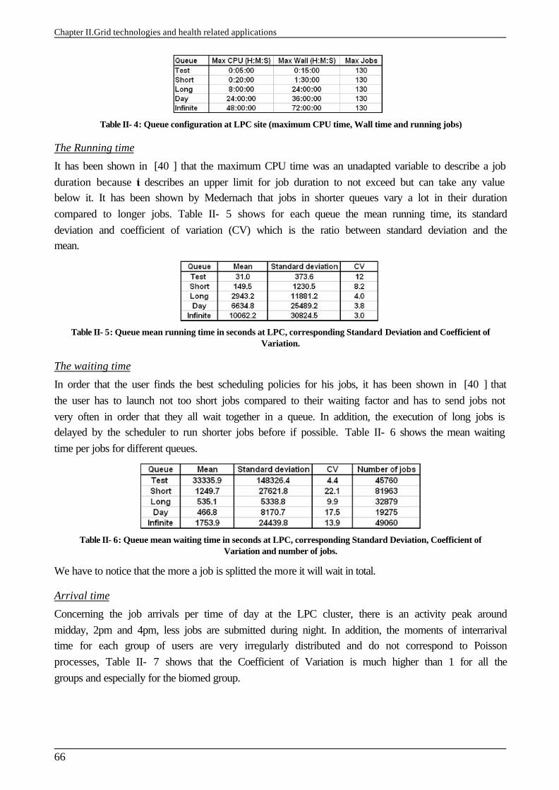
Chapter II.Grid technologies and health related applications
66
Table II- 4: Queue configuration at LPC site (maximum CPU time, Wall time and running jobs)
The Running time
It has been shown in [40 ] that the maximum CPU time was an unadapted variable to describe a job duration because it describes an upper limit for job duration to not exceed but can take any value below it. It has been shown by Medernach that jobs in shorter queues vary a lot in their duration compared to longer jobs. Table II- 5 shows for each queue the mean running time, its standard deviation and coefficient of variation (CV) which is the ratio between standard deviation and the mean.
Table II- 5: Queue mean running time in seconds at LPC, corresponding Standard Deviation and Coefficient of Variation.
The waiting time
In order that the user finds the best scheduling policies for his jobs, it has been shown in [40 ] that the user has to launch not too short jobs compared to their waiting factor and has to send jobs not very often in order that they all wait together in a queue. In addition, the execution of long jobs is delayed by the scheduler to run shorter jobs before if possible. Table II- 6 shows the mean waiting time per jobs for different queues.
Table II- 6: Queue mean waiting time in seconds at LPC, corresponding Standard Deviation, Coefficient of Variation and number of jobs.
We have to notice that the more a job is splitted the more it will wait in total.
Arrival time
Concerning the job arrivals per time of day at the LPC cluster, there is an activity peak around midday, 2pm and 4pm, less jobs are submitted during night. In addition, the moments of interrarival time for each group of users are very irregularly distributed and do not correspond to Poisson processes, Table II- 7 shows that the Coefficient of Variation is much higher than 1 for all the groups and especially for the biomed group.
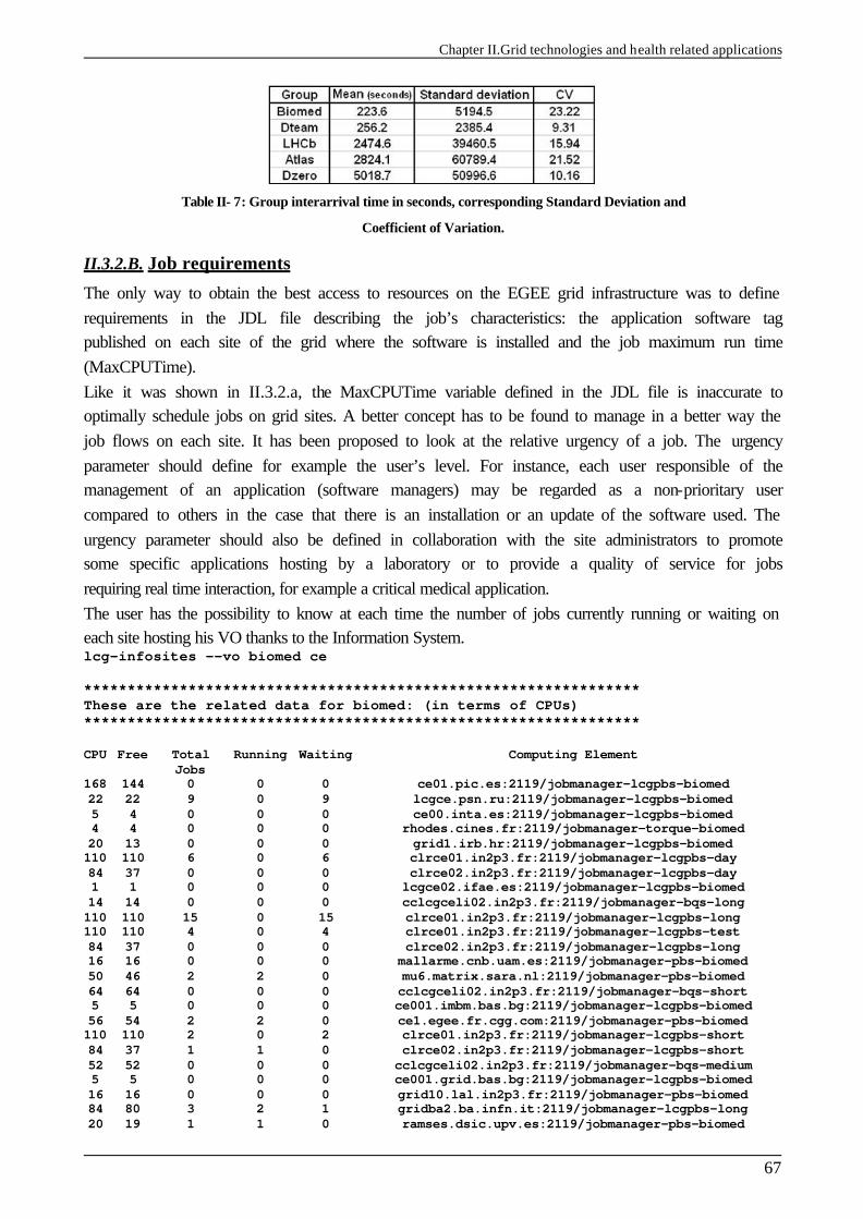
Chapter II.Grid technologies and health related applications
67
Table II- 7: Group interarrival time in seconds, corresponding Standard Deviation and
Coefficient of Variation.
II.3.2.B. Job requirements
The only way to obtain the best access to resources on the EGEE grid infrastructure was to define requirements in the JDL file describing the job’s characteristics: the application software tag published on each site of the grid where the software is installed and the job maximum run time (MaxCPUTime). Like it was shown in II.3.2.a, the MaxCPUTime variable defined in the JDL file is inaccurate to optimally schedule jobs on grid sites. A better concept has to be found to manage in a better way the job flows on each site. It has been proposed to look at the relative urgency of a job. The urgency parameter should define for example the user’s level. For instance, each user responsible of the management of an application (software managers) may be regarded as a non-prioritary user compared to others in the case that there is an installation or an update of the software used. The urgency parameter should also be defined in collaboration with the site administrators to promote some specific applications hosting by a laboratory or to provide a quality of service for jobs requiring real time interaction, for example a critical medical application. The user has the possibility to know at each time the number of jobs currently running or waiting on each site hosting his VO thanks to the Information System. lcg-infosites --vo biomed ce **************************************************************** These are the related data for biomed: (in terms of CPUs) **************************************************************** CPU Free Total
Jobs Running Waiting Computing Element
168 144 0 0 0 ce01.pic.es:2119/jobmanager-lcgpbs-biomed 22 22 9 0 9 lcgce.psn.ru:2119/jobmanager-lcgpbs-biomed 5 4 0 0 0 ce00.inta.es:2119/jobmanager-lcgpbs-biomed 4 4 0 0 0 rhodes.cines.fr:2119/jobmanager-torque-biomed 20 13 0 0 0 grid1.irb.hr:2119/jobmanager-lcgpbs-biomed 110 110 6 0 6 clrce01.in2p3.fr:2119/jobmanager-lcgpbs-day 84 37 0 0 0 clrce02.in2p3.fr:2119/jobmanager-lcgpbs-day 1 1 0 0 0 lcgce02.ifae.es:2119/jobmanager-lcgpbs-biomed 14 14 0 0 0 cclcgceli02.in2p3.fr:2119/jobmanager-bqs-long 110 110 15 0 15 clrce01.in2p3.fr:2119/jobmanager-lcgpbs-long 110 110 4 0 4 clrce01.in2p3.fr:2119/jobmanager-lcgpbs-test 84 37 0 0 0 clrce02.in2p3.fr:2119/jobmanager-lcgpbs-long 16 16 0 0 0 mallarme.cnb.uam.es:2119/jobmanager-pbs-biomed 50 46 2 2 0 mu6.matrix.sara.nl:2119/jobmanager-pbs-biomed 64 64 0 0 0 cclcgceli02.in2p3.fr:2119/jobmanager-bqs-short 5 5 0 0 0 ce001.imbm.bas.bg:2119/jobmanager-lcgpbs-biomed 56 54 2 2 0 ce1.egee.fr.cgg.com:2119/jobmanager-pbs-biomed 110 110 2 0 2 clrce01.in2p3.fr:2119/jobmanager-lcgpbs-short 84 37 1 1 0 clrce02.in2p3.fr:2119/jobmanager-lcgpbs-short 52 52 0 0 0 cclcgceli02.in2p3.fr:2119/jobmanager-bqs-medium 5 5 0 0 0 ce001.grid.bas.bg:2119/jobmanager-lcgpbs-biomed 16 16 0 0 0 grid10.lal.in2p3.fr:2119/jobmanager-pbs-biomed 84 80 3 2 1 gridba2.ba.infn.it:2119/jobmanager-lcgpbs-long 20 19 1 1 0 ramses.dsic.upv.es:2119/jobmanager-pbs-biomed
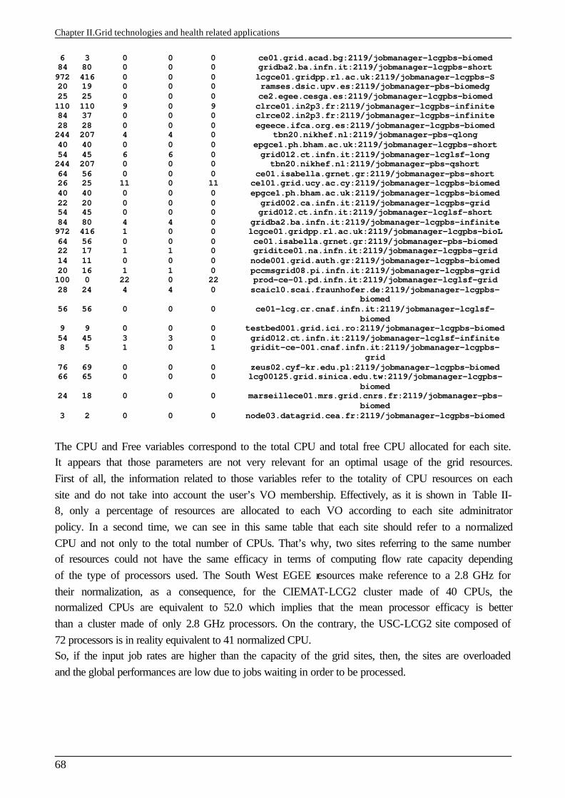
Chapter II.Grid technologies and health related applications
68
6 3 0 0 0 ce01.grid.acad.bg:2119/jobmanager-lcgpbs-biomed 84 80 0 0 0 gridba2.ba.infn.it:2119/jobmanager-lcgpbs-short 972 416 0 0 0 lcgce01.gridpp.rl.ac.uk:2119/jobmanager-lcgpbs-S 20 19 0 0 0 ramses.dsic.upv.es:2119/jobmanager-pbs-biomedg 25 25 0 0 0 ce2.egee.cesga.es:2119/jobmanager-lcgpbs-biomed 110 110 9 0 9 clrce01.in2p3.fr:2119/jobmanager-lcgpbs-infinite 84 37 0 0 0 clrce02.in2p3.fr:2119/jobmanager-lcgpbs-infinite 28 28 0 0 0 egeece.ifca.org.es:2119/jobmanager-lcgpbs-biomed 244 207 4 4 0 tbn20.nikhef.nl:2119/jobmanager-pbs-qlong 40 40 0 0 0 epgce1.ph.bham.ac.uk:2119/jobmanager-lcgpbs-short 54 45 6 6 0 grid012.ct.infn.it:2119/jobmanager-lcglsf-long 244 207 0 0 0 tbn20.nikhef.nl:2119/jobmanager-pbs-qshort 64 56 0 0 0 ce01.isabella.grnet.gr:2119/jobmanager-pbs-short 26 25 11 0 11 ce101.grid.ucy.ac.cy:2119/jobmanager-lcgpbs-biomed 40 40 0 0 0 epgce1.ph.bham.ac.uk:2119/jobmanager-lcgpbs-biomed 22 20 0 0 0 grid002.ca.infn.it:2119/jobmanager-lcgpbs-grid 54 45 0 0 0 grid012.ct.infn.it:2119/jobmanager-lcglsf-short 84 80 4 4 0 gridba2.ba.infn.it:2119/jobmanager-lcgpbs-infinite 972 416 1 0 0 lcgce01.gridpp.rl.ac.uk:2119/jobmanager-lcgpbs-bioL 64 56 0 0 0 ce01.isabella.grnet.gr:2119/jobmanager-pbs-biomed 22 17 1 1 0 griditce01.na.infn.it:2119/jobmanager-lcgpbs-grid 14 11 0 0 0 node001.grid.auth.gr:2119/jobmanager-lcgpbs-biomed 20 16 1 1 0 pccmsgrid08.pi.infn.it:2119/jobmanager-lcgpbs-grid 100 0 22 0 22 prod-ce-01.pd.infn.it:2119/jobmanager-lcglsf-grid 28 24 4 4 0 scaicl0.scai.fraunhofer.de:2119/jobmanager-lcgpbs-
biomed 56 56 0 0 0 ce01-lcg.cr.cnaf.infn.it:2119/jobmanager-lcglsf-
biomed 9 9 0 0 0 testbed001.grid.ici.ro:2119/jobmanager-lcgpbs-biomed 54 45 3 3 0 grid012.ct.infn.it:2119/jobmanager-lcglsf-infinite 8 5 1 0 1 gridit-ce-001.cnaf.infn.it:2119/jobmanager-lcgpbs-
grid 76 69 0 0 0 zeus02.cyf-kr.edu.pl:2119/jobmanager-lcgpbs-biomed 66 65 0 0 0 lcg00125.grid.sinica.edu.tw:2119/jobmanager-lcgpbs-
biomed 24 18 0 0 0 marseillece01.mrs.grid.cnrs.fr:2119/jobmanager-pbs-
biomed 3 2 0 0 0 node03.datagrid.cea.fr:2119/jobmanager-lcgpbs-biomed
The CPU and Free variables correspond to the total CPU and total free CPU allocated for each site. It appears that those parameters are not very relevant for an optimal usage of the grid resources. First of all, the information related to those variables refer to the totality of CPU resources on each site and do not take into account the user’s VO membership. Effectively, as it is shown in Table II- 8, only a percentage of resources are allocated to each VO according to each site adminitrator policy. In a second time, we can see in this same table that each site should refer to a normalized CPU and not only to the total number of CPUs. That’s why, two sites referring to the same number of resources could not have the same efficacy in terms of computing flow rate capacity depending of the type of processors used. The South West EGEE resources make reference to a 2.8 GHz for their normalization, as a consequence, for the CIEMAT-LCG2 cluster made of 40 CPUs, the normalized CPUs are equivalent to 52.0 which implies that the mean processor efficacy is better than a cluster made of only 2.8 GHz processors. On the contrary, the USC-LCG2 site composed of 72 processors is in reality equivalent to 41 normalized CPU. So, if the input job rates are higher than the capacity of the grid sites, then, the sites are overloaded and the global performances are low due to jobs waiting in order to be processed.
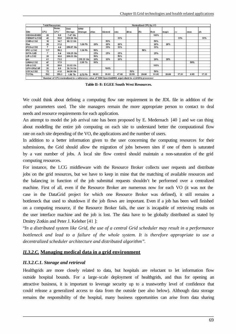
Chapter II.Grid technologies and health related applications
69
Table II- 8: EGEE South West Resources.
We could think about defining a computing flow rate requirement in the JDL file in addition of the other parameters used. The site managers remain the more appropriate person to contact to deal needs and resource requirements for each application. An attempt to model the job arrival rate has been proposed by E. Medernach [40 ] and we can thing about modelling the entire job computing on each site to understand better the computational flow rate on each site depending of the VO, the applications and the number of users. In addition to a better information given to the user concerning the computing resources for their submissions, the Grid should allow the migration of jobs between sites if one of them is saturated by a vast number of jobs. A local site flow control should maintain a non-saturation of the grid computing resources. For instance, the LCG middleware with the Resource Broker collects user requests and distribute jobs on the grid resources, but we have to keep in mine that the matching of available resources and the balancing in function of the job submittal requests shouldn’t be performed over a centralized machine. First of all, even if the Resource Broker are numerous now for each VO (it was not the case in the DataGrid project for which one Resource Broker was defined), it still remains a bottleneck that used to shutdown if the job flows are important. Even if a job has been well finished on a computing resource, if the Resource Broker fails, the user is incapable of retrieving results on the user interface machine and the job is lost. The data have to be globally distributed as stated by Dmitry Zotkin and Peter J. Keleher [41 ]: “In a distributed system like Grid, the use of a central Grid scheduler may result in a performance bottleneck and lead to a failure of the whole system. It is therefore appropriate to use a decentralized scheduler architecture and distributed algorithm”.
II.3.2.C. Managing medical data in a grid environment
II.3.2.C.1. Storage and retrieval
Healthgrids are more closely related to data, but hospitals are reluctant to let information flow outside hospital bounds. For a large-scale deployment of healthgrids, and thus for opening an attractive business, it is important to leverage security up to a trustworthy level of confidence that could release a generalized access to data from the outside (see also below). Although data storage remains the responsibility of the hospital, many business opportunities can arise from data sharing
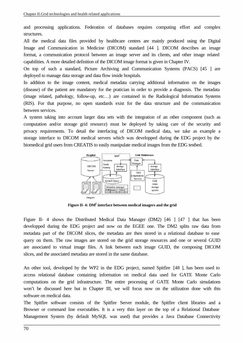
Chapter II.Grid technologies and health related applications
70
and processing applications. Federation of databases requires computing effort and complex structures. All the medical data files provided by healthcare centres are mainly produced using the Digital Image and Communication in Medicine (DICOM) standard [44 ]. DICOM describes an image format, a communication protocol between an image server and its clients, and other image related capabilities. A more detailed definition of the DICOM image format is given in Chapter IV. On top of such a standard, Picture Archiving and Communication Systems (PACS) [45 ] are deployed to manage data storage and data flow inside hospitals. In addition to the image content, medical metadata carrying additional information on the images (disease) of the patient are mandatory for the pratician in order to provide a diagnosis. The metadata (image related, pathology, follow-up, etc…) are contained in the Radiological Information Systems (RIS). For that purpose, no open standards exist for the data structure and the communication between services. A system taking into account larger data sets with the integration of an other component (such as computation and/or storage grid resource) must be deployed by taking care of the security and privacy requirements. To detail the interfacing of DICOM medical data, we take as example a storage interface to DICOM medical servers which was developped during the EDG project by the biomedical grid users from CREATIS to easily manipulate medical images from the EDG testbed.
Figure II- 4: DM2 interface between medical imagers and the grid
Figure II- 4 shows the Distributed Medical Data Manager (DM2) [46 ] [47 ] that has been developped during the EDG project and now on the EGEE one. The DM2 splits raw data from metadata part of the DICOM slices, the metadata are then stored in a relational database to ease query on them. The raw images are stored on the grid storage resources and one or several GUID are associated to virtual image files. A link between each image GUID, the composing DICOM slices, and the associated metadata are stored in the same database. An other tool, developed by the WP2 in the EDG project, named Spitfire [48 ], has been used to access relational database containing information on medical data used for GATE Monte Carlo computations on the grid infrastructure. The entire processing of GATE Monte Carlo simulations won’t be discussed here but in Chapter III, we will focus now on the utilization done with this software on medical data. The Spitfire software consists of the Spitfire Server module, the Spitfire client libraries and a Browser or command line executables. It is a very thin layer on the top of a Relational Database Management System (by default MySQL was used) that provides a Java Database Connectivity
Chapter II.Grid technologies and health related applications
71
driver. It’s using Web Service technology (Jakarta Tomcat) to provide connections to a few user-definable database operations. Spitfire gives a quick an easy access to data, but it is not supposed to be used as a full-fledged Data Management System. The access patterns have to be simple: single or few row lookups and inserts, updates and deletes and information on the tables. Spitfire makes use of the Grid Authentication (X.509 certificates) and an additional authorization. Furthermore, management of distributed databases and data mining capabilities are important tools for many biomedical applications in fields such epidemiology, drug design or even diagnosis. Expert system services running on the grid must be able to interrogate large distributed databases to extract such knowledge as may lead to the early detection of new sources of diseases, risk populations, evolution of diseases or suitable proteins to fight against specific diseases.
II.3.2.C.2. Security and privacy
Security in grid infrastructures is currently adequate for research platforms, but it must be improved in the future to ensure privacy of data in real healthgrids. In order to convince physicians and patients to use grids for their data storage and processing needs, many functionalities need to be provided such as: § Reliable authentication of users § Secure transfer of data between grid elements § Secure storage of data on a grid element § Anonymization of medical records § Access control for resources (data, storage space or computing power) § Tamper-proof logging of operations performed on medical files § Robustness against denial-of-service attacks
The grid infrastructure is able now to answer some requirements for a biomedical usage of the resources, we will detail below what is the status of the grid technologies. Concerning the authentication of users: This subject is well adressed in grid environment. The use of a public key infrastructure (PKI) with certification authorities (CA) and X.509 certificates are sufficient to access the grid resources. The EGEE middleware relies on Globus [13 ] and its public key-based infrastructure [38 ] to answer those needs. Concerning the secure transfer of data: the grid benefits of well researched area such as SSL/TLS, IpSec or SSH and GridFTP for data transfers [49 ]. The EGEE middleware uses this last technology but not yet the encrypted protocol included in. Concerning the secure storage of data: Encrypted storage systems exist but fail to adhere to the dynamic nature of grid access permissions. Mechanisms have to be elaborated to share the decryption keys between users authorized to access data. A solution has been deployed by Seitz et al. [46 ] to provide access to decryption keys based on access permissions. Concerning anonymization: Failure on privacy in biomedical personal information causes irreparable damage, since there is no way to retrieve the situation. Even if the name and address of the patient are removed on the medical file, it is still possible to re-identified the patient using secondary information. A promising approach to deal with anonymisation is described in [50 ].
Chapter II.Grid technologies and health related applications
72
Concerning Authorization and access control: In addition to the cross-organizational nature of grid access permissions, the medical field adds other inherent problems, the confidentiality and a restricted access to data for users part of the same VO. Effectively, the membership of users within those groups must be clarified to have a restricted access to data. Concerning traceability: The grid must provide a log-keeping system enabling the update of information about access requests on the medical data located on the storage element. Concerning the availability of services: measures to prevent denial-of-service attacks are not specific to grid architectures. One thing to keep in mind is that the security services shouldn’t be relied on a single centralized service. Grid technologies can ease the access to replicated resources and information, just requiring the user to have a permanent Internet connection.
CONCLUSION The EDG project was a pioneer in identifying the biomedical domain as a relevant area of application for grid technologies. Conferences and workshops organized in the biomedical domain, with the creation of international entities such as the HealthGrid association or the GGF Life Science research group [52 ] aim to federate research projects and communities in this field. The EGEE project hosts a lot of biomedical applications in which GATE is a pilot deployment, benefiting of the experience gained in the EDG project. As we described it, the functionalities of the Grid are numerous but remain often unadapted to a usage of the grid in clinical routine in addition to the biomedical research needs. The best usage of the grid capabilities has to be found to obtain a sufficient gain in time for the computation of GATE treatment plannings. In the following chapter, we will concentrate on the set up of GATE applications in such Grid infrastructure and the convenient tools developed to enable an inexperienced grid user (physician, medical physicist…) to use the Monte Carlo accuracy in medical treatment planning. The parallelisation of the simulations associated to computing time tests, the data management associated to the usage of medical images in treatment planning, the outputs analysis and a web portal user interface are one of the fields treated. A joint submission between two grid infrastructures, the DEISA and EGEE projects is the next issue to test advantage of supercomputing calculations in medical physics treatment planning.
References [1 ] European Union's Information Society Technologies (IST) research
http://www.cordis.lu/ist/results [2 ] EDG (2001). European DataGrid IST project, FP5, jan. 2001-feb. 2004,
http://www.edg.org/. [3 ] GridLab
http://www.gridlab.org/ [4 ] EUROGrid
http://www.eurogrid.org/ [5 ] CROSSGrid
http://www.crossgrid.org/ [6 ] DATATAG
http://datatag.web.cern.ch/datatag/ [7 ] GEANT
http://www.geant.net/

Chapter II.Grid technologies and health related applications
73
[8 ] EGEE (2004). European IST project of the FP6, Enabling Grids for E-science and industry in Europe, apr. 2004-mar. 2006, http://www.eu-egee.org/.
[9 ] EGEE Middleware Architecture and Planning (Release 1), https://edms.cern.ch/document/476451, 26 August, 2004.
[10 ] DEISA (2004), European IST project of the FP6, http://www.deisa.org/
[11 ] GGF, Global Grid Forum http://www.gridforum.org/
[12 ] UNICORE, Uniform Interface to Computing Resources http://unicore.sourceforge.net/
[13 ] Foster, I. and Kesselman, C. (1997). Globus: A Metacomputing Infrastructure Toolkit. International Journal of Supercomputer Applications , 11(2):115-128.
[14 ] LCG-1 User Guide http://grid-deployment.web.cern.ch/grid-deployment/eis/docs/LCG-1-UserGuide.htm
[15 ] LHC Computing Grid Project http://lcg.web.cern.ch/LCG/
[16 ] LCG User Developer Guide http://grid-deployment.web.cern.ch/grid-deployment/cgi-bin/index.cgi?var=eis/docs
[17 ] LCG Middleware Developers Guide http://grid-deployment.web.cern.ch/grid-deployment/cgi-bin/index.cgi?var=documentation
[18 ] The EDG-Brokerinfo User Guide - Release 2.x. 6th August 2003 http://server11.infn.it/workload-grid/docs/edg-brokerinfo-user-guide -v2 2.pdf
[19 ] Workload Management Software – GUI User Guide. Nov 24th, 2003 http://server11.infn.it/workload-grid/docs/DataGrid-01-TEN-0143-0 0.pdf
[20 ] User Guide for the EDG Local Replica Catalog 2.1.x http://edg-wp2.web.cern.ch/edg-wp2/replication/docu/r2.1/edg-lrc-userguide.pdf
[21 ] User Guide for the EDG Replica Metadata Catalog 2.1.x http://edg-wp2.web.cern.ch/edg-wp2/replication/docu/r2.1/edg-rmc-userguide.pdf
[22 ] User Guide for the EDG Replica Optimization Service 2.1.x http://edg-wp2.web.cern.ch/edg-wp2/replication/docu/r2.1/edg-ros-userguide.pdf
[23 ] User Guide for the Replica Location Index 2.1.x http://edg-wp2.web.cern.ch/edg-wp2/replication/docu/r2.1/edg-rli-userguide.pdf
[24 ] The GLUE schema http://www.cnaf.infn.it/˜sergio/datatag/glue/
[25 ] The Virtual Data Toolkit VDT http://www.cs.wisc.edu/vdt/
[26 ] gLite [27 ] AliEn
http://alien.cern.ch [28 ] The Condor Project.
http://www.cs.wisc.edu/condor/ [29 ] NorduGrid
http://www.nordugrid.org [30 ] ARDA, Architectural Roadmap for Distributed Analysis
http://cern.ch/arda [31 ] GSIFTP Tools for the Data Grid http://www.globus.org/datagrid/deliverables/gsiftp-tools.html [32 ] RFIO: Remote File Input/Output
http://doc.in2p3.fr/doc/public/products/rfio/rfio.html [33 ] MDS (Monitoring and Discovery Service) 2.2 Features in the Globus Toolkit 2.2 Release
http://www.globus.org/mds/ [34 ] Job Description language HowTo. December 17th, 2001
http://server11.infn.it/workload-grid/docs/DataGrid-01-TEN-0102-0 2-Document.pdf [35 ] JDL Attributes – Release 2.x. Oct 28th, 2003
http://server11.infn.it/workload-grid/docs/DataGrid-01-TEN-0142-0 2.pdf [36 ] Classified Advertisements. Condor.
http://www.cs.wisc.edu/condor/classad [37 ] Foster, I., Kesselman, C., and Tuecke, S. (2001). The Anatomy of the Grid: Enabling Scalable
Chapter II.Grid technologies and health related applications
74
Virtual Organizations. International Journal of Supercomputer Applications , 15(3). [38 ] Foster, I., Kesselman, C., Tsudik, G., and Tuecke, S. (1998). A Security Architecture for
Computational Grids. In Proc. 5th ACM Conference on Computer and Communications Security Conference, pages 83{92, San Francisco, CA, USA.
[39 ] EU Grid PMA http://www.eugridpma.org/
[40 ] E. Medernach, Workload Analysis of a cluster in a Grid Environment, OICMS proceedings, June 2005.
[41 ] D. Zotkin, P.J. Keleher. Job length estimation and performance in backfilling schedulers. In HPDC, 1999.
[42 ] V. Breton, K. Dean and T. Solomonides, The HealthGrid White Paper. From Grid to HealthGrid, IOS Press 2005.
[43 ] HealthGrid (2003). HealthGrid Association, http://www.healthgrid.org/. [44 ] DICOM (1996). Digital Imaging and COmmunications in Medicine,
http://medical.nema.org/. [45 ] Huang, H. K. (1996). PACS: Picture Archiving and Communication Systems in Biomedical
Imaging. Hardcover. [46 ] Seitz L., Pierson J., and Brunie L. (2003a). Key management for encrypted data storage in
distributed systems. In Proceedings of the second Security In Storage Workshop (SISW). [47 ] Seitz, L., Pierson, J., and Brunie, L. (2003b). Semantic access control for medical applications in
grid environments. In Euro-Par 2003 Parallel Processing, volume LNCS 2790, pages 374-383. Springer.
[48 ] Spitfire http://edg-wp2.web.cern.ch/edg-wp2/spitfire
[49 ] Allcock, B., Bester, J., Bresnahan, J., Chervenak, A., Foster, I., Kesselman, C., Meder, S., Nefedova, V., Quesnal, D., and Tuecke, S. (2002). Data Management and Transfer in High Performance Computational Grid Environments. Parallel Computing Journal, 28(5):749-771.
[50 ] Claerhout, B. and De Moor, G. (2004). Privacy protection for healthgrid applications. to appear in the Methods of Information in Medcine journal.
[51 ] “Medical images simulations, storage, and processing, on the European DataGrid testbed”, J. Montagnat, F. Bellet, H. Benoit-Cattin, V. Breton, L. Brunie, H. Duque, Y. Legré, I.E. Magnin, L. Maigne, S. Miguet, J.-M. Pierson, L. Seitz, T. Tweed, Journal of Grid Computing, 2004.
[52 ] LSG-RG. Global Grid Forum Life Sciences Grid Research Group (2003) http://forge.gridforum.org/projects/lsg-rg.
Chapter III. The GATE Monte Carlo simulation platform for dosimetric applications
75
Chapter III.
The GATE Monte Carlo simulation platform for dosimetric applications INTRODUCTION GATE (Geant4 Application for Tomographic Emission) is born in December 2001 thanks to a joint effort between the University of Lausanne (Christian Morel and Daniel Strul), the University of Geneva (Giovanni Santin) and the LPC of Clermont-Ferrand (Vincent Breton and Delphine Lazaro). Since, OpenGATE meeting occur three times per year to discuss about the validations and the new developments of the platform. The OpenGATE collaboration published a joint paper in the journal Physics in Medicine in Biology [1 ] in 2004 relating all the implementations and features of the platform. At this date, three sub-working groups have been created inside the OpenGATE collaboration to focus on special fields related in particularly to dosimetric applications: the optimisation of the code, the parallelization of simulations on cluster and/or grid environment and the customization and validation of the platform for dosimetric studies. Effectively, in addition to an ease of use, a Monte Carlo code has to offer a compromise between time consuming and precision of the calculations in order to be used in clinical routine. Furthermore, the Monte Carlo code must be validated for dosimetric applications using in particularly electrons in water equivalent medium and in heterogeneous media (body and tumour volumes reconstructed using CT data). As the definition of the GATE platform has been widely described in some publications and thesis [2 ], we will discuss in a first part on the current functionalities and the requirements necessary to enable the use of GATE for dosimetric applications. A second part is intended to current and future developments enabling: § an efficient usage of the code infrastructure with the implementation of variance reduction
techniques, § the convivial visualization of CT data imported in the simulation, § an extended usage of the platform for dosimetric applications involving dose calculations
based on voxelized volumes (CT data).
Chapter III. The GATE Monte Carlo simulation platform for dosimetric applications
76
§ The validation of the GEANT4 electromagnetic processes implying electrons is detailed in a third part.
III.1. GATE: A MONTE CARLO PLATFORM FOR DOSIMETRY
III.1.1. Functionalities available and requirements for dosimetry applications GATE (Geant4 Application for Tomographic Emission) has been released for the first time in May 2004, with the production of the first open source package of the platform. The last version available is 1.1.0 compatible with GEANT4 version 6.2.p02. Version 1.2.0 compatible with GEANT4 version 7.0.p01 is under test at this date. The platform is encoded in C++ langage on the top of the GEANT4 software. The Scientific Linux 3.0 is the operating system used. The ease of use of the platform is enabled thanks to a scripted interface, all the encoding functionalities of GATE have been transcripted in command lines. The user only needs to call the script line related to the creation of a geometry, output format chosen, etc, to create his simulation.
III.1.1.A. Geometry and Systems
III.1.1.A.1. Existing functionalities
A lot of functionalities in the code are intended to nuclear medicine simulations, for example PET and SPECT system validations and image processing. Creation and definition of geometry (shape, dimensions, material allocated to, translation and rotation, repeaters) are very easy using the GATE command lines. In addition, predefined detector geometry systems are there to facilitate the hierarchical description of a tomograph. Each system can be described by components organized in a tree level structure, each component having its own specific role or ordering. As for an example of the cylindricalPET scanner system, the geometrical volumes containing crystals are grouped in matrices, themselves assembled in submodules and modules. At the top level of this structure, the sectors composed of modules are “repeated” on a cylindrical surface to build up the whole device. The main property of a system is that its geometry description is supported by specific list-mode or histogrammed (sinogram or projection) data output formats. Currently there are five systems available in GATE: one for SPECT, three for PET and a generic system appropriate to model novel tomographic paradigms.
III.1.1.A.2. Needed functionalities
To create specific geometry, for example an iodine brachytherapy source for wich rounded tips are positionned on each side of its cylinder shape, the user has to combine a cylindrical shape and two hemispherical tips joined to it by taking care that volumes don’t overlap between each other. In the same way, ophthalmic applicators with notches are impossible to create using this technique. GATE don’t integrate yet in its functionalities boolean operations that allow the creation of a new volume by the association of two others, nor the BREPS (Boundary Represented Solids) that enables the definition of volumes by describing their boundaries. Both topics are available in the GEANT4 software. Even if the creation of geometry is simple using command lines, GATE has to provide facilities to create complex geometry shapes for radiotherapy and brachytherapy experiments in order to be
Chapter III. The GATE Monte Carlo simulation platform for dosimetric applications
77
used for clinical routine treatments.In the case of dosimetry studies using linear accelerators or brachytherapy sources, the current system used is the generic system “scanner”. Five level components are associated to this system with no geometry fixed as it is the case for example with cylindricalPET system for which a box is allocated to each system components. As no system has been specifically created for linear accelerator nor for brachytherapy geometry building, the user has to post-analyze information concerning interactions occuring in each medium of interest which involves a considerable loss of time. Because geometrical concepts are common to many different linear accelerators, we could imagine to prefine a system for their hierarchical description. We could envisage the same for iodine brachytherapy sources and 106Ru/106Rh ophthalmic applicators.
III.1.1.B. Voxelized sources and phantoms: GATE calculations based on CT data
The current GATE versions enable the simulation of dosimetric studies in voxelized volumes such like CT data. The way to transcript the medical data to insert it in the simulation is quite simple. Two files are needed for the transcription of the medical data in the simulations: a binary file (image.raw) grouping the CT slices and a transcription file (range.dat) to assign to each voxel or, to a range of voxels material characteristics. In the following subparts we will talk about the medical images format that we have to deal with to perform Monte Carlo simulations with voxelized media: the DICOM and Interfile formats.
III.1.1.B.1. Definition of DICOM and Interfile formats
The DICOM standard
Medical images provided by hospitals or clinical centres are defined in the DICOM standard. DICOM, “Digital Imaging and Communication in Medicine” is a norm defining communication methods for the different medical imaging equipments. This norm has been developed to: § Promote communication of digital image information, regardless of device manufacturer § Facilitate the development and expansion of Picture Archiving and Communication Systems
(PACS) that can also interface with other systems of hospital information. § Allow the creation of diagnostic information data bases that can be interrogated by a wide
variety of devices distributed geographically.
DICOM has been emitted by the American College of Radiology (ACR), American College of Cardiology (ACC), American Society of Echocardiography (ASE), European Society of Cardiology (ESC), and American Society of Nuclear Cardiology (ASNC) in association with the NEMA (National Electrical Manufacturers Association) in 1984, and it was originally called the ACR/NEMA standard. This norm is currently updated by those two comittees with the help of international experts like the Japaneese Industry Association for Radiation Apparatus (JIRA) in Japan, and the Committé Européen de Normalisation (CEN TC 251) under the name MEDICOM in Europe. ACR is responsible for technical and medical instructions, whereas the role of the NEMA is dedicated to publications and legal issues to avoid infractions against anti-trust laws.
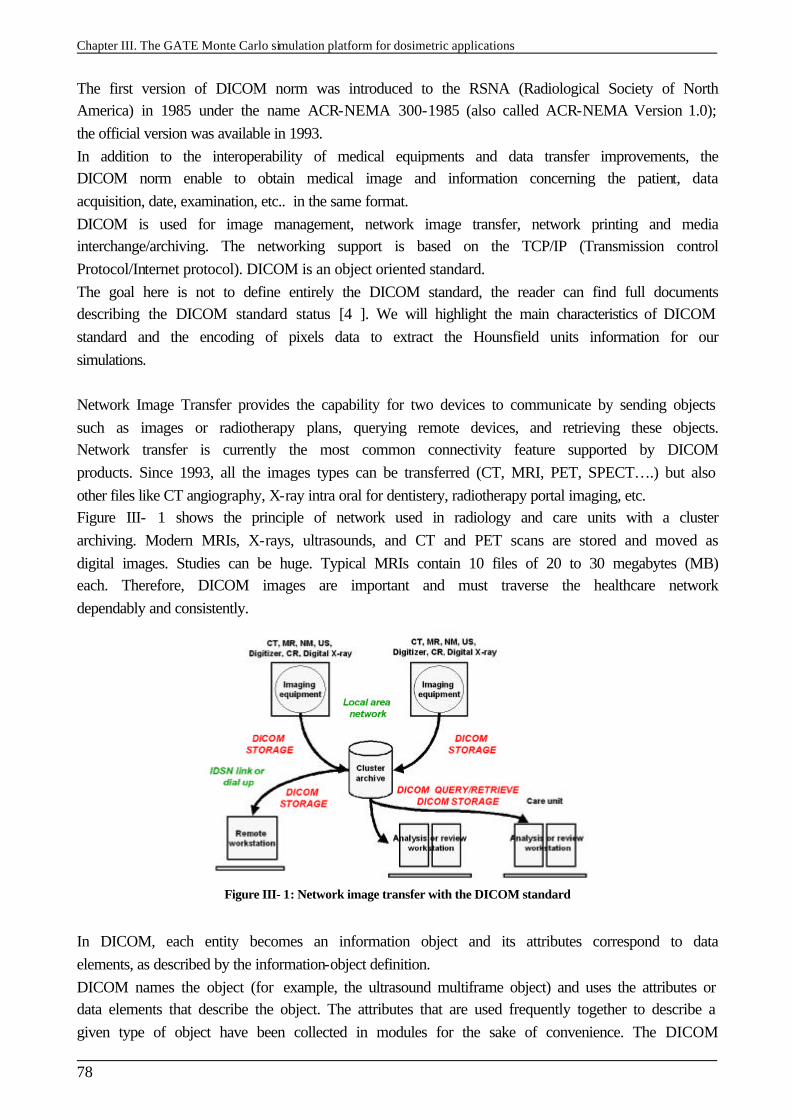
Chapter III. The GATE Monte Carlo simulation platform for dosimetric applications
78
The first version of DICOM norm was introduced to the RSNA (Radiological Society of North America) in 1985 under the name ACR-NEMA 300-1985 (also called ACR-NEMA Version 1.0); the official version was available in 1993. In addition to the interoperability of medical equipments and data transfer improvements, the DICOM norm enable to obtain medical image and information concerning the patient, data acquisition, date, examination, etc.. in the same format. DICOM is used for image management, network image transfer, network printing and media interchange/archiving. The networking support is based on the TCP/IP (Transmission control Protocol/Internet protocol). DICOM is an object oriented standard. The goal here is not to define entirely the DICOM standard, the reader can find full documents describing the DICOM standard status [4 ]. We will highlight the main characteristics of DICOM standard and the encoding of pixels data to extract the Hounsfield units information for our simulations. Network Image Transfer provides the capability for two devices to communicate by sending objects such as images or radiotherapy plans, querying remote devices, and retrieving these objects. Network transfer is currently the most common connectivity feature supported by DICOM products. Since 1993, all the images types can be transferred (CT, MRI, PET, SPECT….) but also other files like CT angiography, X-ray intra oral for dentistery, radiotherapy portal imaging, etc. Figure III- 1 shows the principle of network used in radiology and care units with a cluster archiving. Modern MRIs, X-rays, ultrasounds, and CT and PET scans are stored and moved as digital images. Studies can be huge. Typical MRIs contain 10 files of 20 to 30 megabytes (MB) each. Therefore, DICOM images are important and must traverse the healthcare network dependably and consistently.
Figure III- 1: Network image transfer with the DICOM standard
In DICOM, each entity becomes an information object and its attributes correspond to data elements, as described by the information-object definition. DICOM names the object (for example, the ultrasound multiframe object) and uses the attributes or data elements that describe the object. The attributes that are used frequently together to describe a given type of object have been collected in modules for the sake of convenience. The DICOM
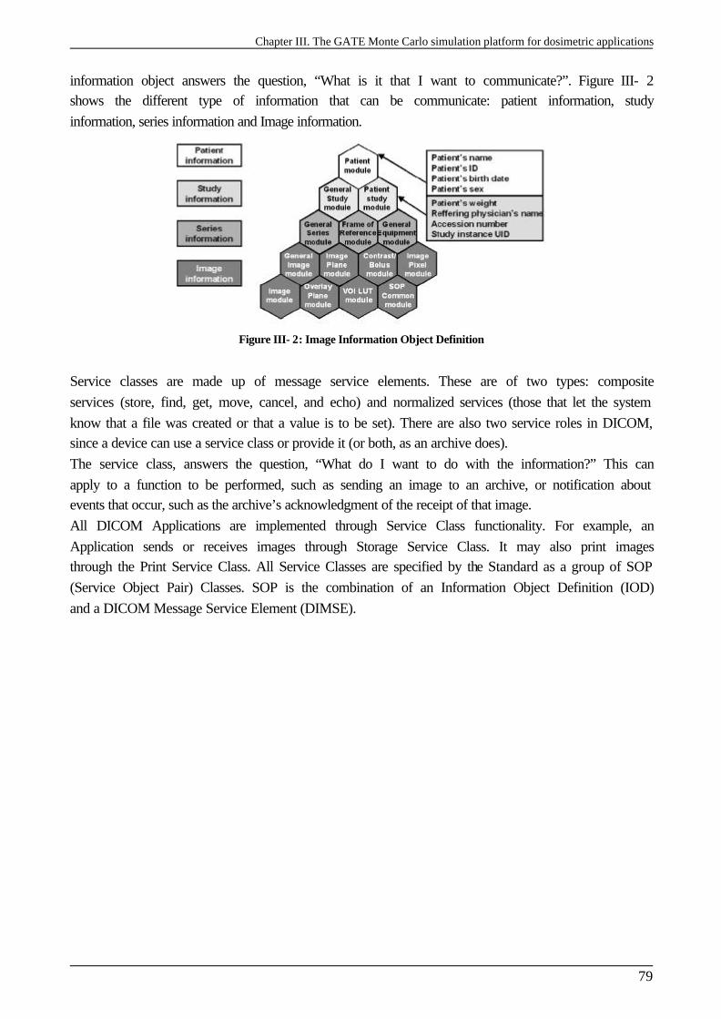
Chapter III. The GATE Monte Carlo simulation platform for dosimetric applications
79
information object answers the question, “What is it that I want to communicate?”. Figure III- 2 shows the different type of information that can be communicate: patient information, study information, series information and Image information.
Figure III- 2: Image Information Object Definition
Service classes are made up of message service elements. These are of two types: composite services (store, find, get, move, cancel, and echo) and normalized services (those that let the system know that a file was created or that a value is to be set). There are also two service roles in DICOM, since a device can use a service class or provide it (or both, as an archive does). The service class, answers the question, “What do I want to do with the information?” This can apply to a function to be performed, such as sending an image to an archive, or notification about events that occur, such as the archive’s acknowledgment of the receipt of that image. All DICOM Applications are implemented through Service Class functionality. For example, an Application sends or receives images through Storage Service Class. It may also print images through the Print Service Class. All Service Classes are specified by the Standard as a group of SOP (Service Object Pair) Classes. SOP is the combination of an Information Object Definition (IOD) and a DICOM Message Service Element (DIMSE).
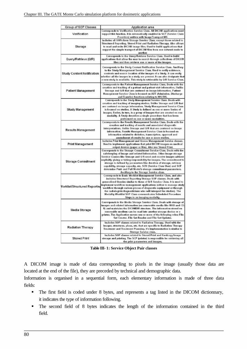
Chapter III. The GATE Monte Carlo simulation platform for dosimetric applications
80
Table III- 1: Service Object Pair classes
A DICOM image is made of data corresponding to pixels in the image (usually those data are located at the end of the file), they are preceded by technical and demographic data. Information is organised in a sequential form, each elementary information is made of three data fields: § The first field is coded under 8 bytes, and represents a tag listed in the DICOM dictionnary,
it indicates the type of information following. § The second field of 8 bytes indicates the length of the information contained in the third
field.
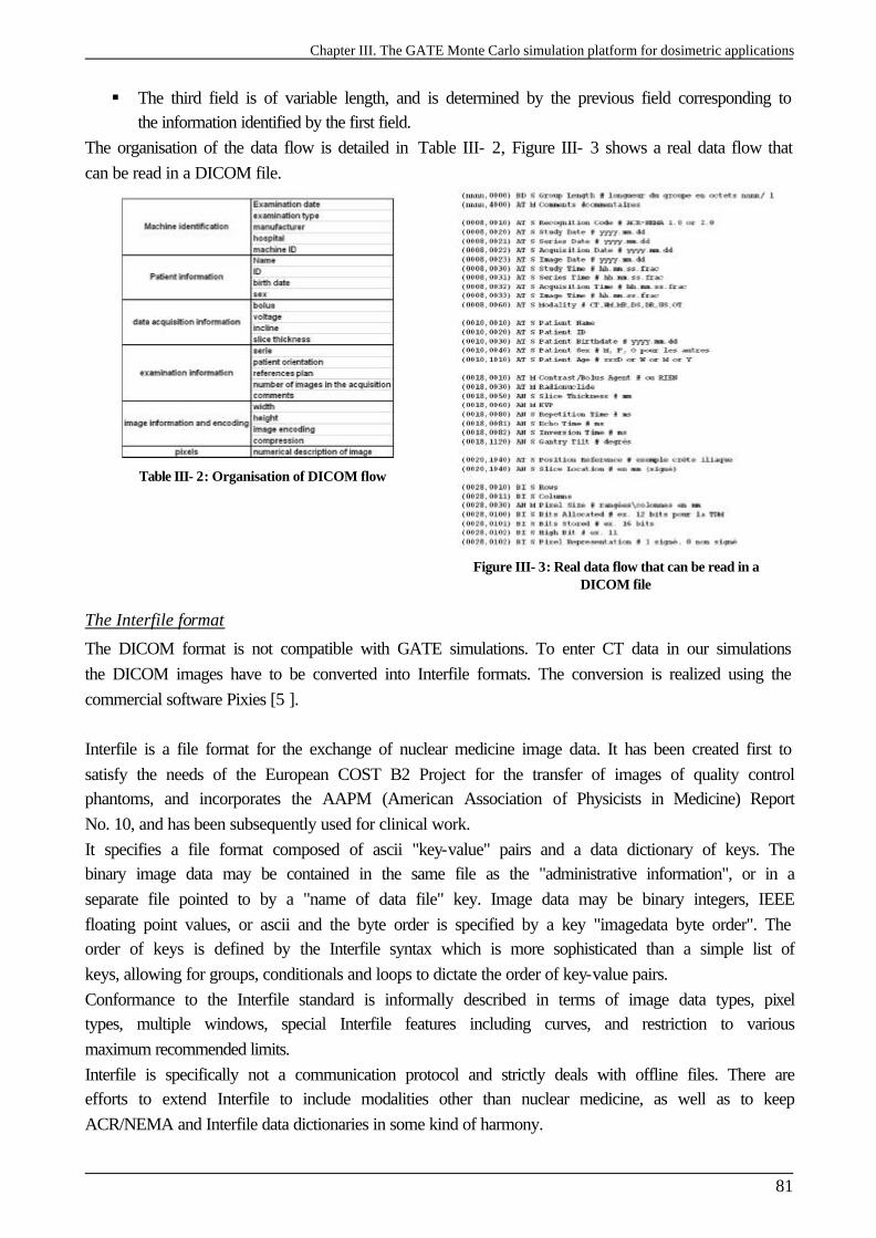
Chapter III. The GATE Monte Carlo simulation platform for dosimetric applications
81
§ The third field is of variable length, and is determined by the previous field corresponding to the information identified by the first field.
The organisation of the data flow is detailed in Table III- 2, Figure III- 3 shows a real data flow that can be read in a DICOM file.
Table III- 2: Organisation of DICOM flow
Figure III- 3: Real data flow that can be read in a DICOM file
The Interfile format
The DICOM format is not compatible with GATE simulations. To enter CT data in our simulations the DICOM images have to be converted into Interfile formats. The conversion is realized using the commercial software Pixies [5 ]. Interfile is a file format for the exchange of nuclear medicine image data. It has been created first to satisfy the needs of the European COST B2 Project for the transfer of images of quality control phantoms, and incorporates the AAPM (American Association of Physicists in Medicine) Report No. 10, and has been subsequently used for clinical work. It specifies a file format composed of ascii "key-value" pairs and a data dictionary of keys. The binary image data may be contained in the same file as the "administrative information", or in a separate file pointed to by a "name of data file" key. Image data may be binary integers, IEEE floating point values, or ascii and the byte order is specified by a key "imagedata byte order". The order of keys is defined by the Interfile syntax which is more sophisticated than a simple list of keys, allowing for groups, conditionals and loops to dictate the order of key-value pairs. Conformance to the Interfile standard is informally described in terms of image data types, pixel types, multiple windows, special Interfile features including curves, and restriction to various maximum recommended limits. Interfile is specifically not a communication protocol and strictly deals with offline files. There are efforts to extend Interfile to include modalities other than nuclear medicine, as well as to keep ACR/NEMA and Interfile data dictionaries in some kind of harmony.
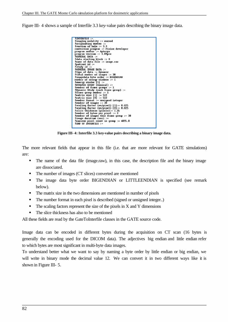
Chapter III. The GATE Monte Carlo simulation platform for dosimetric applications
82
Figure III- 4 shows a sample of Interfile 3.3 key-value pairs describing the binary image data.
Figure III- 4: Interfile 3.3 key-value pairs describing a binary image data.
The more relevant fields that appear in this file (i.e. that are more relevant for GATE simulations) are: § The name of the data file (image.raw), in this case, the description file and the binary image
are dissociated. § The number of images (CT slices) converted are mentioned § The image data byte order BIGENDIAN or LITTLEENDIAN is specified (see remark
below). § The matrix size in the two dimensions are mentioned in number of pixels § The number format in each pixel is described (signed or unsigned integer..) § The scaling factors represent the size of the pixels in X and Y dimensions § The slice thickness has also to be mentioned
All these fields are read by the GateToInterfile classes in the GATE source code. Image data can be encoded in different bytes during the acquisition on CT scan (16 bytes is generally the encoding used for the DICOM data). The adjectives big endian and little endian refer to which bytes are most significant in multi-byte data images. To understand better what we want to say by naming a byte order by little endian or big endian, we will write in binary mode the decimal value 12. We can convert it in two different ways like it is shown in Figure III- 5.
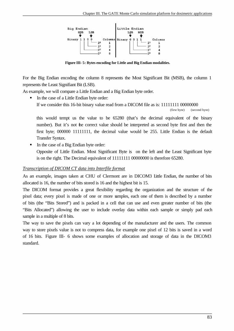
Chapter III. The GATE Monte Carlo simulation platform for dosimetric applications
83
Figure III- 5: Bytes encoding for Little and Big Endian modalities.
For the Big Endian encoding the column 8 represents the Most Significant Bit (MSB), the column 1 represents the Least Signifiant Bit (LSB). As example, we will compare a Little Endian and a Big Endian byte order. § In the case of a Little Endian byte order:
If we consider this 16-bit binary value read from a DICOM file as is: 11111111 00000000 (first byte) (second byte)
this would tempt us the value to be 65280 (that’s the decimal equivalent of the binary number). But it’s not the correct value should be interpreted as second byte first and then the first byte; 000000 11111111, the decimal value would be 255. Little Endian is the default Transfer Syntax.
§ In the case of a Big Endian byte order: Opposite of Little Endian. Most Significant Byte is on the left and the Least Significant byte is on the right. The Decimal equivalent of 11111111 00000000 is therefore 65280.
Transcription of DICOM CT data into Interfile format
As an example, images taken at CHU of Clermont are in DICOM3 Little Endian, the number of bits allocated is 16, the number of bits stored is 16 and the highest bit is 15. The DICOM format provides a great flexibility regarding the organization and the structure of the pixel data; every pixel is made of one or more samples, each one of them is described by a number of bits (the “Bits Stored”) and is packed in a cell that can use and even greater number of bits (the “Bits Allocated”) allowing the user to include overlay data within each sample or simply pad each sample in a multiple of 8 bits. The way to save the pixels can vary a lot depending of the manufacturer and the users. The common way to store pixels value is not to compress data, for example one pixel of 12 bits is saved in a word of 16 bits. Figure III- 6 shows some examples of allocation and storage of data in the DICOM3 standard.
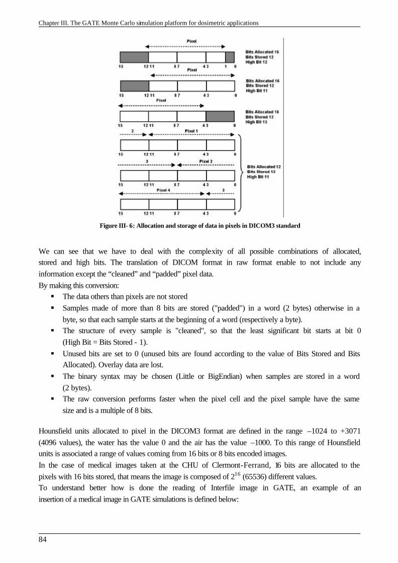
Chapter III. The GATE Monte Carlo simulation platform for dosimetric applications
84
Figure III- 6: Allocation and storage of data in pixels in DICOM3 standard
We can see that we have to deal with the complexity of all possible combinations of allocated, stored and high bits. The translation of DICOM format in raw format enable to not include any information except the “cleaned” and “padded” pixel data. By making this conversion: § The data others than pixels are not stored § Samples made of more than 8 bits are stored ("padded") in a word (2 bytes) otherwise in a
byte, so that each sample starts at the beginning of a word (respectively a byte). § The structure of every sample is "cleaned", so that the least significant bit starts at bit 0
(High Bit = Bits Stored - 1). § Unused bits are set to 0 (unused bits are found according to the value of Bits Stored and Bits
Allocated). Overlay data are lost. § The binary syntax may be chosen (Little or BigEndian) when samples are stored in a word
(2 bytes). § The raw conversion performs faster when the pixel cell and the pixel sample have the same
size and is a multiple of 8 bits. Hounsfield units allocated to pixel in the DICOM3 format are defined in the range –1024 to +3071 (4096 values), the water has the value 0 and the air has the value –1000. To this range of Hounsfield units is associated a range of values coming from 16 bits or 8 bits encoded images. In the case of medical images taken at the CHU of Clermont-Ferrand, 16 bits are allocated to the pixels with 16 bits stored, that means the image is composed of 216 (65536) different values. To understand better how is done the reading of Interfile image in GATE, an example of an insertion of a medical image in GATE simulations is defined below:
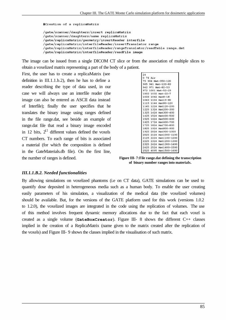
Chapter III. The GATE Monte Carlo simulation platform for dosimetric applications
85
The image can be issued from a single DICOM CT slice or from the association of multiple slices to obtain a voxelized matrix representing a part of the body of a patient. First, the user has to create a replicaMatrix (see definition in III.1.1.b.2), then he has to define a reader describing the type of data used, in our case we will always use an interfile reader (the image can also be entered as ASCII data instead of Interfile); finally the user specifies that he translates the binary image using ranges defined in the file range.dat, see beside an example of range.dat file that read a binary image encoded in 12 bits, 212 different values defined the voxels CT numbers. To each range of bits is associated a material (for which the composition is defined in the GateMaterials.db file). On the first line, the number of ranges is defined.
Figure III- 7:File range.dat defining the transcription of binary number ranges into materials.
III.1.1.B.2. Needed functionalities
By allowing simulations on voxelized phantoms (i.e on CT data), GATE simulations can be used to quantify dose deposited in heterogeneous media such as a human body. To enable the user creating easily parameters of his simulation, a visualization of the medical data (the voxelized volumes) should be available. But, for the versions of the GATE platform used for this work (versions 1.0.2 to 1.2.0), the voxelized images are integrated in the code using the replication of volumes. The use of this method involves frequent dynamic memory allocations due to the fact that each voxel is created as a single volume (GateBoxCreator). Figure III- 8 shows the different C++ classes implied in the creation of a ReplicaMatrix (name given to the matrix created after the replication of the voxels) and Figure III- 9 shows the classes implied in the visualisation of such matrix.
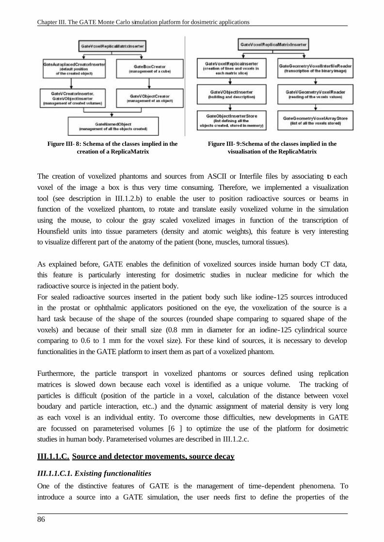
Chapter III. The GATE Monte Carlo simulation platform for dosimetric applications
86
Figure III- 8: Schema of the classes implied in the creation of a ReplicaMatrix
Figure III- 9:Schema of the classes implied in the visualisation of the ReplicaMatrix
The creation of voxelized phantoms and sources from ASCII or Interfile files by associating to each voxel of the image a box is thus very time consuming. Therefore, we implemented a visualization tool (see description in III.1.2.b) to enable the user to position radioactive sources or beams in function of the voxelized phantom, to rotate and translate easily voxelized volume in the simulation using the mouse, to colour the gray scaled voxelized images in function of the transcription of Hounsfield units into tissue parameters (density and atomic weights), this feature is very interesting to visualize different part of the anatomy of the patient (bone, muscles, tumoral tissues). As explained before, GATE enables the definition of voxelized sources inside human body CT data, this feature is particularly interesting for dosimetric studies in nuclear medicine for which the radioactive source is injected in the patient body. For sealed radioactive sources inserted in the patient body such like iodine-125 sources introduced in the prostat or ophthalmic applicators positioned on the eye, the voxelization of the source is a hard task because of the shape of the sources (rounded shape comparing to squared shape of the voxels) and because of their small size (0.8 mm in diameter for an iodine-125 cylindrical source comparing to 0.6 to 1 mm for the voxel size). For these kind of sources, it is necessary to develop functionalities in the GATE platform to insert them as part of a voxelized phantom. Furthermore, the particle transport in voxelized phantoms or sources defined using replication matrices is slowed down because each voxel is identified as a unique volume. The tracking of particles is difficult (position of the particle in a voxel, calculation of the distance between voxel boudary and particle interaction, etc..) and the dynamic assignment of material density is very long as each voxel is an individual entity. To overcome those difficulties, new developments in GATE are focussed on parameterised volumes [6 ] to optimize the use of the platform for dosimetric studies in human body. Parameterised volumes are described in III.1.2.c.
III.1.1.C. Source and detector movements, source decay
III.1.1.C.1. Existing functionalities
One of the distinctive features of GATE is the management of time-dependent phenomena. To introduce a source into a GATE simulation, the user needs first to define the properties of the
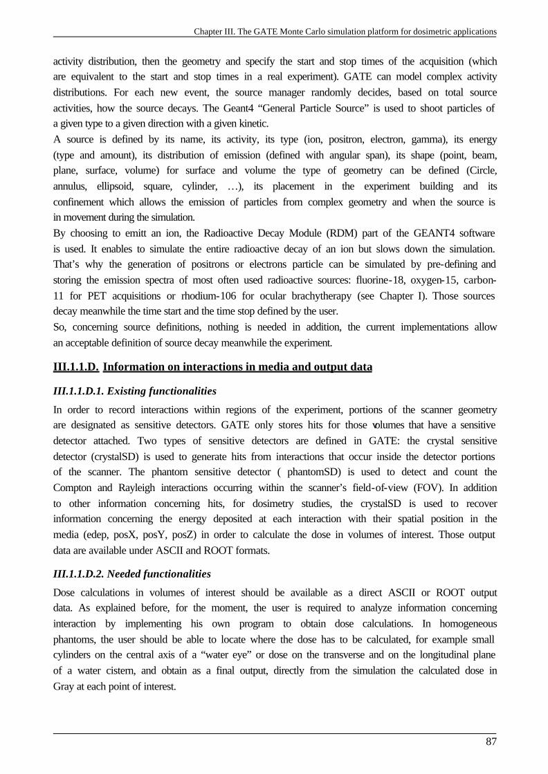
Chapter III. The GATE Monte Carlo simulation platform for dosimetric applications
87
activity distribution, then the geometry and specify the start and stop times of the acquisition (which are equivalent to the start and stop times in a real experiment). GATE can model complex activity distributions. For each new event, the source manager randomly decides, based on total source activities, how the source decays. The Geant4 “General Particle Source” is used to shoot particles of a given type to a given direction with a given kinetic. A source is defined by its name, its activity, its type (ion, positron, electron, gamma), its energy (type and amount), its distribution of emission (defined with angular span), its shape (point, beam, plane, surface, volume) for surface and volume the type of geometry can be defined (Circle, annulus, ellipsoid, square, cylinder, …), its placement in the experiment building and its confinement which allows the emission of particles from complex geometry and when the source is in movement during the simulation. By choosing to emitt an ion, the Radioactive Decay Module (RDM) part of the GEANT4 software is used. It enables to simulate the entire radioactive decay of an ion but slows down the simulation. That’s why the generation of positrons or electrons particle can be simulated by pre-defining and storing the emission spectra of most often used radioactive sources: fluorine-18, oxygen-15, carbon-11 for PET acquisitions or rhodium-106 for ocular brachytherapy (see Chapter I). Those sources decay meanwhile the time start and the time stop defined by the user. So, concerning source definitions, nothing is needed in addition, the current implementations allow an acceptable definition of source decay meanwhile the experiment.
III.1.1.D. Information on interactions in media and output data
III.1.1.D.1. Existing functionalities
In order to record interactions within regions of the experiment, portions of the scanner geometry are designated as sensitive detectors. GATE only stores hits for those volumes that have a sensitive detector attached. Two types of sensitive detectors are defined in GATE: the crystal sensitive detector (crystalSD) is used to generate hits from interactions that occur inside the detector portions of the scanner. The phantom sensitive detector ( phantomSD) is used to detect and count the Compton and Rayleigh interactions occurring within the scanner’s field-of-view (FOV). In addition to other information concerning hits, for dosimetry studies, the crystalSD is used to recover information concerning the energy deposited at each interaction with their spatial position in the media (edep, posX, posY, posZ) in order to calculate the dose in volumes of interest. Those output data are available under ASCII and ROOT formats.
III.1.1.D.2. Needed functionalities
Dose calculations in volumes of interest should be available as a direct ASCII or ROOT output data. As explained before, for the moment, the user is required to analyze information concerning interaction by implementing his own program to obtain dose calculations. In homogeneous phantoms, the user should be able to locate where the dose has to be calculated, for example small cylinders on the central axis of a “water eye” or dose on the transverse and on the longitudinal plane of a water cistern, and obtain as a final output, directly from the simulation the calculated dose in Gray at each point of interest.
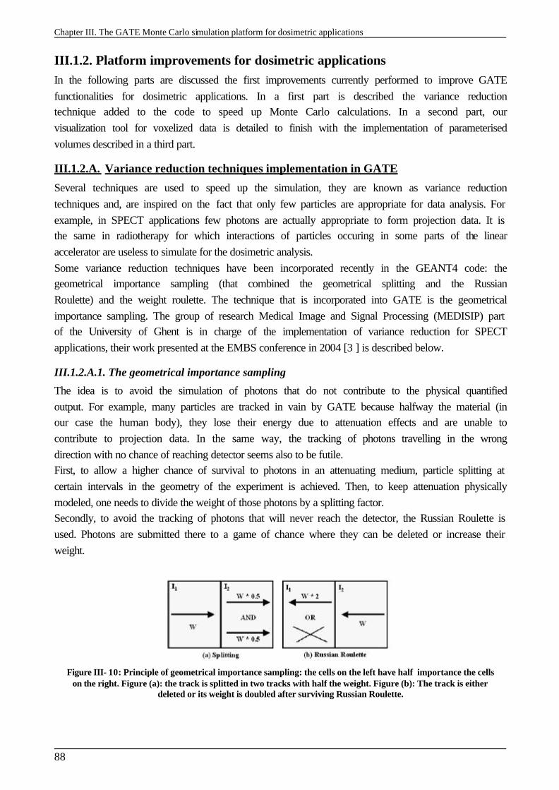
Chapter III. The GATE Monte Carlo simulation platform for dosimetric applications
88
III.1.2. Platform improvements for dosimetric applications In the following parts are discussed the first improvements currently performed to improve GATE functionalities for dosimetric applications. In a first part is described the variance reduction technique added to the code to speed up Monte Carlo calculations. In a second part, our visualization tool for voxelized data is detailed to finish with the implementation of parameterised volumes described in a third part.
III.1.2.A. Variance reduction techniques implementation in GATE
Several techniques are used to speed up the simulation, they are known as variance reduction techniques and, are inspired on the fact that only few particles are appropriate for data analysis. For example, in SPECT applications few photons are actually appropriate to form projection data. It is the same in radiotherapy for which interactions of particles occuring in some parts of the linear accelerator are useless to simulate for the dosimetric analysis. Some variance reduction techniques have been incorporated recently in the GEANT4 code: the geometrical importance sampling (that combined the geometrical splitting and the Russian Roulette) and the weight roulette. The technique that is incorporated into GATE is the geometrical importance sampling. The group of research Medical Image and Signal Processing (MEDISIP) part of the University of Ghent is in charge of the implementation of variance reduction for SPECT applications, their work presented at the EMBS conference in 2004 [3 ] is described below.
III.1.2.A.1. The geometrical importance sampling
The idea is to avoid the simulation of photons that do not contribute to the physical quantified output. For example, many particles are tracked in vain by GATE because halfway the material (in our case the human body), they lose their energy due to attenuation effects and are unable to contribute to projection data. In the same way, the tracking of photons travelling in the wrong direction with no chance of reaching detector seems also to be futile. First, to allow a higher chance of survival to photons in an attenuating medium, particle splitting at certain intervals in the geometry of the experiment is achieved. Then, to keep attenuation physically modeled, one needs to divide the weight of those photons by a splitting factor. Secondly, to avoid the tracking of photons that will never reach the detector, the Russian Roulette is used. Photons are submitted there to a game of chance where they can be deleted or increase their weight.
Figure III- 10: Principle of geometrical importance sampling: the cells on the left have half importance the cells on the right. Figure (a): the track is splitted in two tracks with half the weight. Figure (b): The track is either
deleted or its weight is doubled after surviving Russian Roulette.
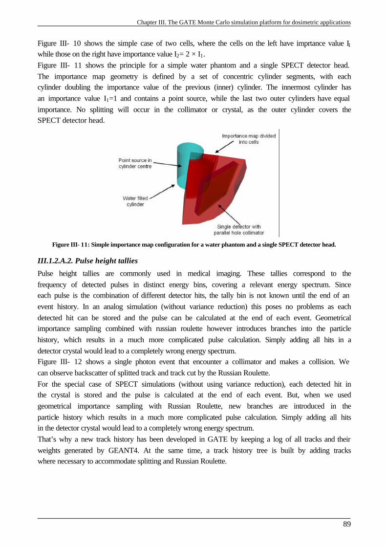
Chapter III. The GATE Monte Carlo simulation platform for dosimetric applications
89
Figure III- 10 shows the simple case of two cells, where the cells on the left have imprtance value I1 while those on the right have importance value I2= 2 × I1. Figure III- 11 shows the principle for a simple water phantom and a single SPECT detector head. The importance map geometry is defined by a set of concentric cylinder segments, with each cylinder doubling the importance value of the previous (inner) cylinder. The innermost cylinder has an importance value I1=1 and contains a point source, while the last two outer cylinders have equal importance. No splitting will occur in the collimator or crystal, as the outer cylinder covers the SPECT detector head.
Figure III- 11: Simple importance map configuration for a water phantom and a single SPECT detector head.
III.1.2.A.2. Pulse height tallies
Pulse height tallies are commonly used in medical imaging. These tallies correspond to the frequency of detected pulses in distinct energy bins, covering a relevant energy spectrum. Since each pulse is the combination of different detector hits, the tally bin is not known until the end of an event history. In an analog simulation (without variance reduction) this poses no problems as each detected hit can be stored and the pulse can be calculated at the end of each event. Geometrical importance sampling combined with russian roulette however introduces branches into the particle history, which results in a much more complicated pulse calculation. Simply adding all hits in a detector crystal would lead to a completely wrong energy spectrum. Figure III- 12 shows a single photon event that encounter a collimator and makes a collision. We can observe backscatter of splitted track and track cut by the Russian Roulette. For the special case of SPECT simulations (without using variance reduction), each detected hit in the crystal is stored and the pulse is calculated at the end of each event. But, when we used geometrical importance sampling with Russian Roulette, new branches are introduced in the particle history which results in a much more complicated pulse calculation. Simply adding all hits in the detector crystal would lead to a completely wrong energy spectrum. That’s why a new track history has been developed in GATE by keeping a log of all tracks and their weights generated by GEANT4. At the same time, a track history tree is built by adding tracks where necessary to accommodate splitting and Russian Roulette.
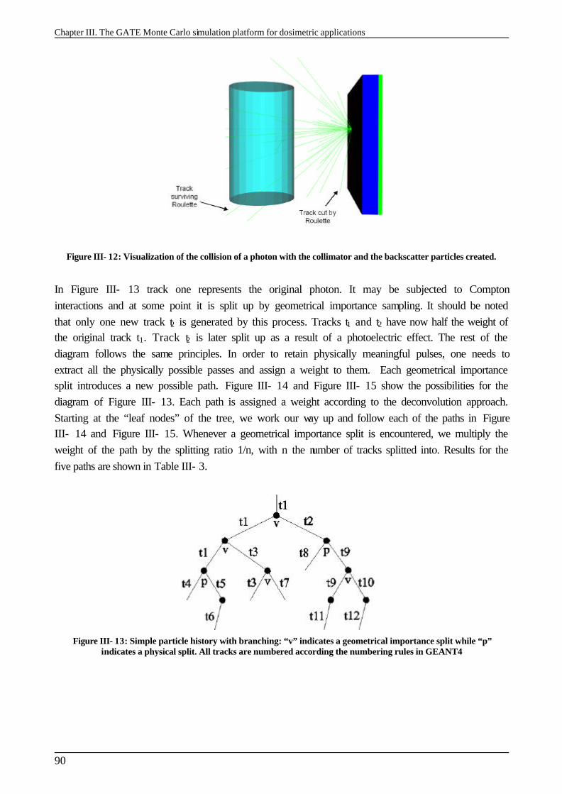
Chapter III. The GATE Monte Carlo simulation platform for dosimetric applications
90
Figure III- 12: Visualization of the collision of a photon with the collimator and the backscatter particles created.
In Figure III- 13 track one represents the original photon. It may be subjected to Compton interactions and at some point it is split up by geometrical importance sampling. It should be noted that only one new track t2 is generated by this process. Tracks t1 and t2 have now half the weight of the original track t1. Track t2 is later split up as a result of a photoelectric effect. The rest of the diagram follows the same principles. In order to retain physically meaningful pulses, one needs to extract all the physically possible passes and assign a weight to them. Each geometrical importance split introduces a new possible path. Figure III- 14 and Figure III- 15 show the possibilities for the diagram of Figure III- 13. Each path is assigned a weight according to the deconvolution approach. Starting at the “leaf nodes” of the tree, we work our way up and follow each of the paths in Figure III- 14 and Figure III- 15. Whenever a geometrical importance split is encountered, we multiply the weight of the path by the splitting ratio 1/n, with n the number of tracks splitted into. Results for the five paths are shown in Table III- 3.
Figure III- 13: Simple particle history with branching: “v” indicates a geometrical importance split while “p” indicates a physical split. All tracks are numbered according the numbering rules in GEANT4
Chapter III. The GATE Monte Carlo simulation platform for dosimetric applications
91
Figure III- 14: Two physically possible branches from the right side of Figure III- 13.
Figure III- 15: Three physically possible branches from the left side of Figure III- 13.
It is now possible to group crystal hits together by simply looking up if they belong to the same ”physical” path and thus form an actual pulse. In this case it could be that only paths 1, 2 and 4 result in actual pulses, but not paths 3 and 5 in Table III- 3 if there are crystal hits tied to paths 1, 2 and 4, but not to paths 3 and 5. Note that the sum of weights of all paths in a track history tree equals 1, thus the total weight is conserved. A track can increase its weight by surviving Russian Roulette. In this case it could be scattered towards a region of higher importance and be subjected to geometrical importance splitting. Figure 6 shows how this is dealt with. The track history adds the same track t1 with its new weight 1 - as it is doubled by Russian Roulette - as a physical branch. This ”new” track acts as a parent for the tracks produced by the splitting which follows in this case and represents in fact the same physical track t1 but with a doubled weight. By adding the track in the history tree in this way, we make sure that a parent track t1 with the appropriate weight can be located for any subsequent tracks.
Table III- 3: The five paths with their respective weight. The sum of weights: 0.25+0.25+0.125=1.
III.1.2.B. Visualisation of medical images in 3 dimensions
The solution was found to create an external module to enable the visualisation of medical images described as Interfile format. The C++ langage has been chosen for the module encoding, the OpenGL has been used for the visualisation part and the display management. This module is compatible with a Linux system (Xlib library). The input data necessary for the visualisation are:
- a file describing the image (info.visu); - the binary image (image.raw); - an ASCII transcription file (range.dat)
Figure III- 16 represents an example of “info.visu” file to describe the medical data to be visualised.
Chapter III. The GATE Monte Carlo simulation platform for dosimetric applications
92
Figure III- 16: File “info.visu” describing the medical data: name of the image,transcription file, number of voxels and their dimensions
All the parameters described in this file are mandatory to visualise the medical data to use in GATE simulations. § The fichierRAW parameter defines the binary image (CT slices) to use. § The fichierRange parameter defines the transcription of the ranges of voxels. § The fichierSortieRAW parameter defines the resulting binary image, after the user
modifications. § The fichierObjets parameter is a file describing the geometries to insert near or inside the
voxelized medical slices. § The fichierSortieObjets parameter is the file created after modifications of the user. § The numCoupe parameter is for describing the number of slices part of the medical binary
image § The numPixelX, numPixelY parameters describe the number of pixels in the X and Y
dimensions in the binary file. § The sizePixelX, sizePixelY, sizePixelZ parameters define the voxel dimensions in the binary
file. The module is composed of two parts: § A dialogue screen describing all the functionalities available: zoom, translation of the slices,
rotation of the slices, coordinate axes, moving on the different slices, adding of a slice, remove of a slice, registration, creation and insertion of volumes.
§ A visualisation screen that shows the voxelized slices to the user.
Figure III- 17 represents a screenshot of the C++ module. Thanks to this visualization tool, we are able to quantify the range of voxels for which we have defined a tissue associated to. Effectively the particularity of the viewer is to enable the coloring of voxels following some range values. The file table.visu allows the user to fix colours to visualize voxels ranges by describing them with a Red Green Blue (RGB) encoding.
Chapter III. The GATE Monte Carlo simulation platform for dosimetric applications
93
Figure III- 17: Screenshot of the C++ module enabling the visualisation of medical data. On the left part, the dialogue screen enable the user to manage the image. On the right part the creen of visualisation
Table III- 4: File table.visu. The color Red (255 0 0) has been assigned to the material Mat19-80 (for
Hounsfield number between 19 and 80 H)
Figure III- 18: Range of materials between 19 and 80 H visualized in red color by the Linux viewer.
Chapter III. The GATE Monte Carlo simulation platform for dosimetric applications
94
III.1.2.C. The parameterised volumes in GATE simulations
III.1.2.C.1. Particle transport in Geant4
Several levels occur in the particle transport : run (initialization, termination, and overall control of running a pre-defined number of histories), event (simulation of one history), track (an intermediate level between event and step), step( advancing one step). The unit of particle propagation is step, i.e, relocation of the particle from the current position to the next position. The G4SteppingManager class is responsible for the management of the particle transport. The GetPhysicalInteractionLength (GPIL) functions of all registered processes for the current type of particle in transport are invoked, and the travelling distance by every process is calculated (for G4Transportation) or sampled (for physics processes). The process with the minimum step length will be selected to be the one to constrain the step size; next, the AlongStepDoIt method of all continuous and continuous-discrete process with the minimum step length and the processes whose PostStepDoIt method will be executed no matter their step length will be invoked. The states of the particle (spatial position, energy, direction, spin, traveling time,etc) are updated during and at the end of each step. The step size is critical for computational efficiency. Due to the continuous energy loss, the step size should be small so that the difference of the cross sections at the beginning and at the end of the step is small enough. On the other hand, the step size cannot be too small in order not to increase the computing time too much.
III.1.2.C.2. Parameterised volume
In GATE (GEANT4) the best volume type for hosting up to tens of millions of CT voxels is a parameterised volume. Parameterised Volumes are repeated volumes in the case in which the multiple copies of a volume can be different in size, solid type, or material. Therefore for CT voxels defined in a parameterised volume, the dimensions and materials can all be different (even if the dimensions of the voxels are the same in CT images, the material allocation can be different for each voxel). A great advantage of parameterised volume is the high efficiency in memory usage. Effectively, in the case of ReplicaMatrix, each rectangular voxel is defined as a single volume (an object of G4Box), therefore the total memory is much larger since we have to save information concerning the mother volume, the name of the voxels and assign material density and composition. For a parameterised volume, although the volume is functionally divided into a certain number of daughter volumes (e.g, CT voxels), there is always only one volume object existent at any given time. This volume is used to represent all the daughter volumes by dynamically changing its properties of volume type, dimensions, location, and material. Each time when a particle encounters the boundary of the current volume, the properties of this volume will be refreshed to reflect those of the next daughter volume the particle will enter. The memory saving with parameterised volume for CT data is tremendous. To define a parameterised volume, the optimized direction X, Y, Z or all three directions have to be chosen to group the voxels in order to improve the transport efficiency. During optimization, the spatial span of each daughter volume along the designated optimization direction in the

Chapter III. The GATE Monte Carlo simulation platform for dosimetric applications
95
parameterised volume is determined. The parameterised volume is then sliced with a thickness of one half of the minimum span. Each daughter volume (CT voxels) in a parameterised volume is given an exclusive index number (copy number) as the identifier, and this number is stored in the corresponding slice vectors. When a particle reaches the parameterised volume from outside, this copy number stored in the slice vector will be examined to find the daughter volume the particle will go into. In the case of the particle is already in the parameterized volume, when a particle arrives at the boundary of a voxel, a new voxel is searched from the vector of the current slice or one of its neighboring slices. When a particle goes from one voxel to another, we have to search the voxel where the particle will enter in. To improve the search mechanism of the voxel without modiying the Geant4 code, is to use one parameterised volume for one CT slice. The selected optimization axis should be parallel to the CT slice. For the case of 512 × 512 voxels per slice, the maximum number of voxels searched each time is 1024.
III.2. VALIDATION OF GEANT4 ELECTROMAGNETIC PHYSICS FOR ELECTRONS
III.2.1. Interactions of electrons Any energy loss process must calculate the continuous and discrete energy loss in a material. Below a given energy threshold the energy loss is continuous and above it the energy loss is simulated by the explicit production of secondary particles. Hard ionisation events generate secondary electrons and hard bremsstrahlung collisions generate secondary photons. The energy loss of the primary and the phase state of the secondary particles is generated by sampling from the appropriate probability density functions decribing the processes. Two processes play an important role in electron interactions with matter: § Inelastic collisions of electrons with atomic electrons: the Möller cross section § Inelastic interaction of electrons with nuclei: Bremsstrahlung
III.2.1.A. Inelastic interaction with atomic electrons: ionization process
When an electron gets inside a medium, interactions with atomic electrons occur. Each of this interaction involves an energy loss Q that can take the value 0 to the cinetic energy of the electron τ. An incident electron is subjected to a lot of interactions before being stopped. This slowing down is caracterised by the linear energy transfer which is the mean energy transferred to the medium (dE) by the electron per unit of length. The Bethe-Bloch formula, caracterising the energy loss per length unit, must be modified in order to take into account the low electron mass involving that the mass of the incident particle (electron) is equal to the mass of the target particle (atomic electron) and the fact that the electrons aren’t distinguishable.
2 4 2
22 20
2
4 ( 2)ln ( )
(4 )2
k
coll e
e
cdE NZ z eF
dx m ZIm c
π τ ττ
πε υ
+ − = × + −
Equation III- 1

Chapter III. The GATE Monte Carlo simulation platform for dosimetric applications
96
with 22
(2 1)ln28( ) 1
( 1)F
ττ
τ βτ
− += − +
+
τ :the cinetic energy of the electron, me: masse of an electron,
/ cβ υ= ,
ck is a correction parameter that depends of energy and of the atomic number Z, I: mean ionisation potential. This quantity is difficult to calculate as it groups the global atomic properties (excitation levels and relative differential cross sections of those excitations). It has been measured for different materials and parameterised in function of Z.
1.19
12 7 / 13/
9.76 58.8 13
Z eV ZI Z
Z eV Z−
+ <=
+ ≥ Equation III- 2
III.2.1.B. Inelastic interaction of electrons with nuclei: Bremsstrahlung
The interaction of a fast electron impiging on a neutral atom involves the curving of the trajectory of the electron under the coulombian force effect; the energy transfered is practically nul. The electron submitted to this acceleration radiates energy by the production of a photon with an energy E deducted from the kinetic energy of the electron. The radiative energy loss is given by
4
2 4 2
( 1) 2 44ln
137 3r e e
dE NEZ Z e Edx m c m c
+ − = −
Equation III- 3
Bombarding electrons can also eject electrons from the inner shells of the atoms of the metal target, and the quick filling of those vacancies by electrons dropping down from higher levels gives rise to sharply defined characteristic x-rays. The energy loss by inelastic collisions is the major process involves in water at the energies used in brachytherapy treatments using electrons. The Bremsstrahlung process is predominant at high energy and for high Z media (approximatively 100 MeV in water and 10 MeV in lead).
III.2.1.C. Electron stopping powers and ranges
§ The maximum range, Rp, is the thickness of absorber at which the recorded transmission reduces to an undetectable level. To measure, it is therefore a rather arbitrary quantity depending on the threshold sensitivity of the detector. Usually it will be larger than the extrapolated range.
§ The extrapolated range Rex, is determined by extrapolation of the linear portion of the transmission curve to the abscissa. For low-energy electrons, because of the occurrence of large energy transfers and angular deviations, Rex is the quantity which, on the available experimental evidence, most closely corresponds to the theoretical RCSDA range in the continuous slowing down approximation (CSDA). The continuous slowing down approximation (CSDA) range represents the path length that an electron would traverse when slowing down from its original energy E to a stop, if its rate of energy loss along the track were equal to the mean rate of energy loss.
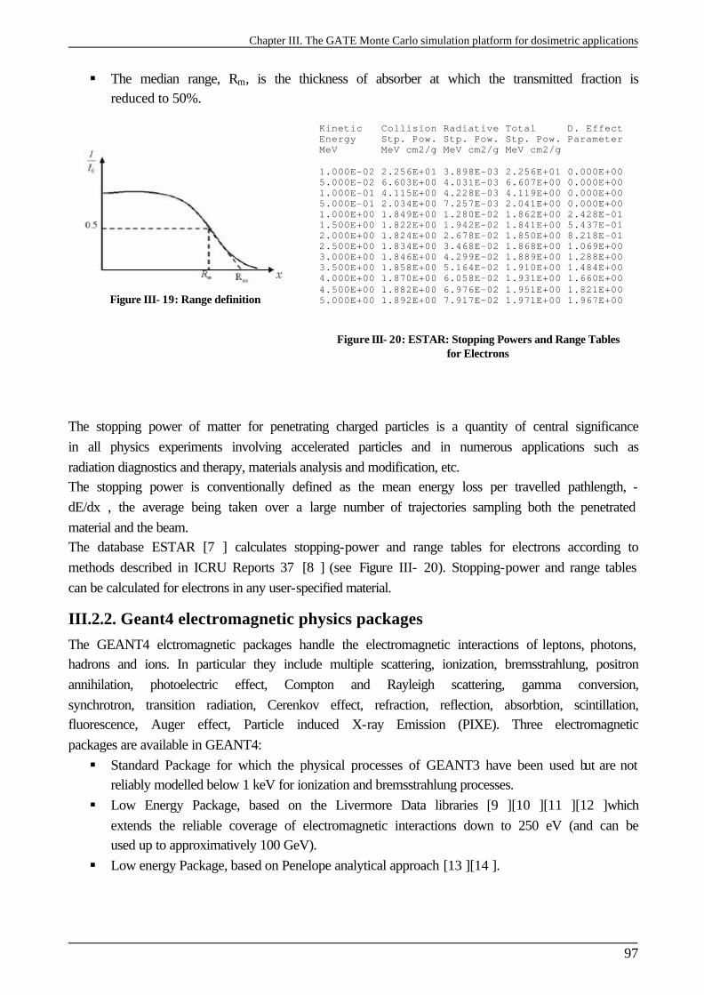
Chapter III. The GATE Monte Carlo simulation platform for dosimetric applications
97
§ The median range, Rm, is the thickness of absorber at which the transmitted fraction is reduced to 50%.
Figure III- 19: Range definition
Kinetic Collision Radiative Total D. Effect Energy Stp. Pow. Stp. Pow. Stp. Pow. Parameter MeV MeV cm2/g MeV cm2/g MeV cm2/g 1.000E-02 2.256E+01 3.898E-03 2.256E+01 0.000E+00 5.000E-02 6.603E+00 4.031E-03 6.607E+00 0.000E+00 1.000E-01 4.115E+00 4.228E-03 4.119E+00 0.000E+00 5.000E-01 2.034E+00 7.257E-03 2.041E+00 0.000E+00 1.000E+00 1.849E+00 1.280E-02 1.862E+00 2.428E-01 1.500E+00 1.822E+00 1.942E-02 1.841E+00 5.437E-01 2.000E+00 1.824E+00 2.678E-02 1.850E+00 8.218E-01 2.500E+00 1.834E+00 3.468E-02 1.868E+00 1.069E+00 3.000E+00 1.846E+00 4.299E-02 1.889E+00 1.288E+00 3.500E+00 1.858E+00 5.164E-02 1.910E+00 1.484E+00 4.000E+00 1.870E+00 6.058E-02 1.931E+00 1.660E+00 4.500E+00 1.882E+00 6.976E-02 1.951E+00 1.821E+00 5.000E+00 1.892E+00 7.917E-02 1.971E+00 1.967E+00
Figure III- 20: ESTAR: Stopping Powers and Range Tables for Electrons
The stopping power of matter for penetrating charged particles is a quantity of central significance in all physics experiments involving accelerated particles and in numerous applications such as radiation diagnostics and therapy, materials analysis and modification, etc. The stopping power is conventionally defined as the mean energy loss per travelled pathlength, -dE/dx , the average being taken over a large number of trajectories sampling both the penetrated material and the beam. The database ESTAR [7 ] calculates stopping-power and range tables for electrons according to methods described in ICRU Reports 37 [8 ] (see Figure III- 20). Stopping-power and range tables can be calculated for electrons in any user-specified material.
III.2.2. Geant4 electromagnetic physics packages The GEANT4 elctromagnetic packages handle the electromagnetic interactions of leptons, photons, hadrons and ions. In particular they include multiple scattering, ionization, bremsstrahlung, positron annihilation, photoelectric effect, Compton and Rayleigh scattering, gamma conversion, synchrotron, transition radiation, Cerenkov effect, refraction, reflection, absorbtion, scintillation, fluorescence, Auger effect, Particle induced X-ray Emission (PIXE). Three electromagnetic packages are available in GEANT4: § Standard Package for which the physical processes of GEANT3 have been used but are not
reliably modelled below 1 keV for ionization and bremsstrahlung processes. § Low Energy Package, based on the Livermore Data libraries [9 ][10 ][11 ][12 ]which
extends the reliable coverage of electromagnetic interactions down to 250 eV (and can be used up to approximatively 100 GeV).
§ Low energy Package, based on Penelope analytical approach [13 ][14 ].

Chapter III. The GATE Monte Carlo simulation platform for dosimetric applications
98
III.2.2.A. The Standard package
The standard package [15 ] provides a variety of models based on an analytical approach to describe the interactions of electrons, positrons, photons and charged hadrons in the enrgy range between 1 keV and 100 TeV. The models assume that the atomic electrons are quasi-free (i.e, their binding energy is neglected except for photoelectric effect) while the atomic nucleus is fixed (i.e., the recoil momentum is negelected).
III.2.2.A.1. The ionization process in the standard package
The G4eIonisation class provides the continuous and discrete energy losses of electrons and positrons due to ionization in a material GEANT4 uses the Möller differential cross section, σM, to treat inelastic collisions of electrons with atomic electrons (e-e-) above a given threshold energy. The Möller cross section, which was derived for collisions with free electrons at rest, is given by
( )( )22
2 2 2
12 1 1 1 2 1 1( , , ) ln
1 2 1e
cutr Z x
Z E T xx x x
γπ γσ
β γ γ γ
− − − = × − + − − − − Equation III- 4
with 2
2 2
2
/
1 (1/ )
/( )cut
E mc
x T E mc
γ
β γ
=
= −
= −
The direction of the ejected electron is generated with respect to the direction of the incident particle. The azimuthal angle φ is generated isotropically and the polar angle θ is calculated from energy-momentum conservation. This information is used to calculate the energy and momentum of both the scattered incident particle and the ejected electron, and to transform them to the global coordinate system.
III.2.2.A.2. The bremsstrahlung process in the standard package
The G4eBremsstrahlung class provides the energy loss of electrons and positrons due to the radiation of photons in the field of a nucleus. Above a given threshold energy the energy loss is simulated by the explicit production of photons. Below the threshold the emission of soft photons is treated as a continuous energy loss. The parameterisation of the energy loss and the total cross section is given in the GEANT4 Physics Reference Manual [16 ].
III.2.2.B. The Low Energy package: evaluated data driven approach
The Low Energy package extends the range of accuracy of electromagnetic interactions down to lower energy than the Standard package. The Low Energy package exploits evaluated data libraries (EPDL97 [9 ], EEDL [10 ], EADL [11 ]) that provide data for the calculation of the cross-sections and the sampling of the final state for the modeling of photon and electron interactions with matter. The current implementation of low energy electron and photon processes can be used down to 250 eV. For now, GATE involves the use of the standard and low energy electromagnetic packages for the photon processes and the standard electromagnetic package only for the processes implying electrons. It adopts different models depending on the energy range and the particle charge. In the
Chapter III. The GATE Monte Carlo simulation platform for dosimetric applications
99
high energy domain (> 2 MeV) the Bethe-Bloch formula, while in the low energy one (< 1 keV for protons) the free electron model are applied respectively. In the intermediate energy range parameterized models based on experimental data from Ziegler [17 ] and ICRU reviews are implemented; corrections due to the molecular structure of materials and the effect of the nuclear stopping power are taken into account.
III.2.2.B.1. The ionization process in the Low Energy package
The sampling method is based on energy spectra of delta rays contained in the EEDL, and the process is treated as a number of discrete interactions. The energy spectrum data are available as a function of sub-shell. Subsequent fluorescence is treated. The class G4LowEnergyIonisation calculates the continuous energy loss due to electron ionisation and simulates δ-ray production by electrons. The δ-electron production threshold for a given material, Tc, is used to separate the continuous and the discrete parts of the process. The energy loss of an electron with the incident energy, T, is expressed via the sum over all atomic shells, s, and the integral over the energy, t, of δ-electrons. The δ-electron production cross-section is a complimentary function:
max
max
0.1
( ) ( )
T
Tcs T
seV
d dtdtT Td dtdt
σ
σ σσ
=
∫∑
∫ Equation III- 5
where Tmax=0.5T is the maximum energy transfered to a δ-electron, σs(T) is the total cross-section for the shell, s, at a given incident kinetic energy, T, and 0.1 eV is the low energy limit of the EEDL data. The probability of emission of a δ-electron with kinetic energy, t, from a sub-shell, s, of binding energy, Bs, as the result of the interaction of an incoming electron with kinetic energy, T, is described by:
2
( ) , s
s
t Bd P x with xdt x T Bσ += =
+ Equation III- 6
where the parameter x is varied from min (0.1 )/( )s sx eV B T B= + + to 0.5. The function, P(x), is parameterised differently in 3 regions of x: from xmin to x1 the linear interpolation with linear scale of 4 points is used; from x1 to x2 the linear interpolation with logarithmic scale of 16 points is used; from x2 to 0.5 the following interpolation is applied:
22 1
( ) 1 (1 ) *(0.5 )/1 1
xP x gx g x g A x x
x x = − + − + − + − − −
Equation III- 7
where A is a fit coefficient, g is expressed via the gamma factor of the incoming electron: 2(2 1) /g γ γ= − Equation III- 8
For the high energy case (x >> 1) the formula of P(x) is transformed to the Möller electron-electron scattering formula. The value of the coefficient, A, for each element is obtained as a result of the fit on the spectrum from the EEDL data for those energies which are available in the database. The values of x1 and x2
Chapter III. The GATE Monte Carlo simulation platform for dosimetric applications
100
are chosen for each atomic shell according to the spectrum of δ-electrons in this shell. Note that x1 corresponds to the maximum of the spectrum, if the maximum does not coincide with xmin. The dependence of all 24 parameters on the incident energy, T, is evaluated from a logarithmic interpolation. The sampling of the final state proceeds in three steps. First a shell is randomly selected, then the energy of the δ-electron is sampled, finally the angle of emission of the scattered electron and of the δ-ray is determined by energy-momentum conservation taken into account electron motion on the atomic orbit. The interaction leaves the atom in an excited state. The deexcitation of the atom is simulated. Sampling of the excitations is carried out for both the continuous and the discrete parts of the process.
III.2.2.B.2. The Bremsstrahlung process in the Low Energy package
The class G4LowEnergyBremsstrahlung calculates the continuous energy loss due to low energy gamma emission and simulates the gamma production by electrons. The gamma production threshold for a given material wc used to separate the continuous and the discrete parts of the process. The energy loss of an electron with the incident energy T re expressed via the integrand over energy of the gammas. The angular distribution of the emitted photons with respect to the incident electron can be sampled according to three alternative generators described below. The direction of the outcoming electron is determined from the energy-momentum balance. These generators are currently implemented in G4ModifiedTsai, G4Generator2BS and G4Generator2BN classes.
III.2.2.C. The Low Energy package: analytic approach
The physics models developed for the Penelope Simulation Toolkit (PENetration and Energy Loss of Positrons and Electrons) [13 ] have been implemented in GEANT4 as an alternative and independent set of processes in the Low Energy Package. The models, specifically developed for Monte Carlo simulation, are based on an approach which combines numerical databases with analytical cross section models for the different interaction mechanisms. In particular, they include low-energy and atomic effects (e.g. Doppler broadening, shell effects) and can be applied to energies from a few hundred eV to about 1 GeV [14 ]. The G4PenelopeIonisation class calculates the continuous energy loss due to electron and positron ionisation and simulates the δ-ray production by electrons and positrons. The electron production threshold Tc for a given material is used to separate the continuous and the discrete parts of the process. The simulation of inelastic collisions of electrons and positrons is performed on the basis of a Generalized Oscillation Strength (GOS) model [18 ]. It is assumed that GOS splits into contributions from the different atomic electron shells. The total cross section σ -(E) for the inelastic collision of electrons of energy is calculated analytically. It can be split into contributions from distant longitudinal, distant transverse and close interactions,
Chapter III. The GATE Monte Carlo simulation platform for dosimetric applications
101
, ,( ) d i s l dist cloEσ σ σ σ− −= + + Equation III- 9
III.2.2.D. Specification of the GEANT4 physic processes in GATE
In GATE, the physical processes specified for electrons and positrons transport are hard coded in the software and can not be altered. User can define the photon processes list (photo-electric effect, Compton scattering, Rayleigh effect and gamma conversion); and for each process, the user can select the specific energy model (standard electromagnetic physics, low energy electromagnetic physics or do not simulate the interaction). For electrons and positrons, the standard electromagnetic package is used. Charged particles are tracked to the end of their range. A cut allows the user to suppress particles whose range would be less than a user defined value that we name the range cut. As a consequence, there is no tracking cuts but only production thresholds. For photons the absorption length defines the cut. GATE allows the choice of three types of cut: the cut concerning secondary electrons (setElectronCut), the cut concerning the delta rays (setDeltaRayCut) and cut for X-rays (setXRayCut). The cuts concerning delta rays and X-rays production are always applied using the low-energy electromagnetic package.
III.2.3. Multiple scattering implementation in GEANT4 In GEANT4, the electron step algorithm is modelled in the multiple scattering process. A brief discussion follows concerning the implementation of the process and the corrected parameters concerning the angular distribution between 5.2.p02, 6.2.p02 and 7.0.p01 GEANT4 versions and the different dosimetric studies obtained as a consequence of these modifications. Multiple Scattering (MSC) simulation algorithms can be classified as either "detailed" or "condensed". In the detailed algorithms, all the collisions/interactions experienced by the particle are simulated. This simulation can be considered as exact; it gives the same results as the solution of the transport equation. However, it can be used only if the number of collisions is not too large, a condition fulfilled only for special geometries (such as thin foils), or low enough kinetic energies. For larger kinetic energies the average number of collisions is very large and the detailed simulation becomes very inefficient. In all condensed history Monte Carlo programs, the effect of the large number of elastic interactions which occur over a given pathlength is modelled by means of a multiple scattering theory; the global effects of the collisions are simulated at the end of a track segment. The global effects generally computed in these codes are the net displacement, energy loss, and change of direction of the charged particle. Most particle physics simulation codes use the multiple scattering theories of Molière [18 ], Goudsmit and Saunderson [20 ] and Lewis [19 ]. The theories of Molière and Goudsmit-Saunderson, which are exact if the cross section remains constant over a step, describe the angular deflection of electrons after travelling a given pathlength. The Lewis theory computes the moments of the spatial distribution as well. None of these MSC theories gives the probability distribution of the spatial displacement. Therefore each of the MSC simulation codes incorporates its own algorithm to determine the spatial displacement of the charged particle after a given step. These

Chapter III. The GATE Monte Carlo simulation platform for dosimetric applications
102
algorithms are not exact, and are responsible for most of the uncertainties in the MSC codes. Therefore the simulation results can depend on the value of the step length and generally one has to select the value of the step length carefully. A new class of MSC simulation, the "mixed" simulation algorithms, appeared in the literature recently. The mixed algorithm simulates the "hard" collisions one by one and uses a MSC theory to treat the effects of the "soft" collisions at the end of a given step. Such algorithms can prevent the number of steps from becoming too large and also reduce the dependence on the step length. As it was stated before, for the majority of photon and electron interaction processes, there are three implementations available: Standard, Low-energy and Penelope. The charged particle multiple scattering process is an exception in which alternative models are not available. The MSC model used in GEANT4 belongs to the class of condensed simulations, class II. The model is based on Lewis' MSC theory and uses model functions to determine the angular and spatial distributions after a step. The functions have been chosen in such a way as to give the same moments of the (angular and spatial) distributions as the Lewis theory. This theory is applicable for all scattering angles, and it allows electron step sizes to be arbitrarily small.
III.2.3.A. The angular distribution
The angular distribution is approximately Gaussian for small scattering angles in both versions, but the width of the distribution has been changed between the versions; the Highland formula has been corrected for the central part of the distribution. There are differences in the tail of the distribution as well.
III.2.3.A.1. The tail of the distribution
GEANT4 version 5.2.p02
In the Geant4 version 5.2.p02, the angular distribution u=cosθ is sampled according to a model function g(u). The functional form of the function is
[ ]1 3 2( ) ( ) (1 ) ( ) (1 ) ( )g u p qg u q g u p g u= + − + − Equation III- 10
where 0 , 1p q≤ ≤ , gi are simple functions of u=cosθ (normalized in [ ]1,1u ∈ − ). These functions have been chosen as
(1 )1 1 0
2 2 0
3 3
( ) 1 1
1( ) 1 1
(1 )( ) 1 1
a u
c
g u C e u u
g u C u uu
g u C u
− −= − ≤ ≤ ≤
= − ≤ ≤ ≤−
= − ≤ ≤
where a>0, c>0 and u0 are model parameters, Ci normalization constants. For small scattering angle θ, g1(u) is close to the Gaussian 2 2
0exp( / 2 )θ θ− with 20 1/ aθ = , while g(u) has a Rutherford-like tail
for large θ, if c is not far from 2.
GEANT4 version 6.2.p02
In the 6.2.p02 version, the g2(u) function as the form
2 21
( )( )c
g u Cb u
=−
with b>0

Chapter III. The GATE Monte Carlo simulation platform for dosimetric applications
103
It involves a modification in the Rutherford-like tail for large θ.
GEANT4 version 7.0.p01 Nothing has been modified in this version concerning the tail of the distribution.
III.2.3.A.2. The width of the angular distribution: correction of the Highland formula
GEANT4 version 5.2.p02
In the 5.2.p02 version, the original Highland-Lynch-Dahl formula is used and give the parameterisation of the central part of the distribution as
0 0 0
13.6/ (1 0.038ln / )
MeVz x X x X
cpθ
β= + Equation III- 11
where θ0 is the width of the approximate Gaussian projected angle distribution, p, βc and z are the momentum, velocity and charge number of the incident particle, and x/X0 is the thickness of the scattering medium in radiation lengths.
GEANT4 version 6.2.p02
In this version, for electrons and positrons, the width given by the Highland formula was bigger than the value observed by Hanson (with 10% of differences at small angles). Therefore, a modified correction term was introduced:
The original correction term 0
1 0.038lnxX
+
has been replaced by a term of the form
2
1 20 0
1 ln lnx x
c cX X
+ +
for x/X0 <1.
The constants c1 and c2 were chosen in such a way that the Hanson data is reproduced in the simulation.
GEANT4 version 7.0.p01
The width of the central part of the distribution has been modified, the modified formula for θ0 is 0.555
0
13.60
MeV xz
cp Xθ
β =
Equation III- 12
This formula gives much smaller step dependence in the angular distribution and describes the available electron scattering data better than the Highland form.
III.2.3.B. The path length correction PLC
In every electron step, a path length correction (PLC) is performed to calculate the energy loss along the step. The PLC refers to the transformation between the electron geometrical path length and the true path length. The geometrical path length is defined as the straight-line distance of the step and the true path length takes into account the path curvature and so, is longer than the geometrical path length. After the electron is transported along its initial geometrical path, the code samples the mean lateral displacement and the scattering angle.
Chapter III. The GATE Monte Carlo simulation platform for dosimetric applications
104
The mean lateral displacement accounts for the lateral deflection of the electron along the step, whereas the scattering angle determines the direction vector of the next step. These two quantities are not correlated in the GEANT4 model. To prevent the step to cross a boundary, a safety radius that corresponds to the distance to the closest boundary, from all directions is compared to the lateral displacement. If the safety radius is smaller, the electron is relocated laterally to a distance equal to the safety. The PLC is not correlated to the scattering angle, and the lateral displacement is switched off when the electron stops at the interface.
III.2.4. The step control and boundary crossing parameters in GEANT4 The particle step length is determined by the volume boundaries, thresholds for secondary particle production and the location of the discrete interaction site. For electrons, the production threshold is specified in terms of range which is then internally converted to energy for every material. The following lines represent the standard output generated by a GEANT4 execution. Production cuts have been fixed to 10 µm for electrons, 1 mm for positrons and 1 µm for photons. The conversion of range in energy is given for the materials used in the simulation, here, there’s Air, Water and Silver materials. ========= Table of registered couples ============================== Index : 0 used in the geometry : Yes recalculation needed : No Material : Air Range cuts : gamma 1 mum e- 10 mum e+ 1 mm Energy thresholds : gamma 990 eV e- 990 eV e+ 990 eV Region(s) which use this couple : DefaultRegionForTheWorld Index : 1 used in the geometry : Yes recalculation needed : No Material : Water Range cuts : gamma 1 mum e- 10 mum e+ 1 mm Energy thresholds : gamma 990 eV e- 6.44974 keV e+ 338.695 keV Region(s) which use this couple : DefaultRegionForTheWorld Index : 2 used in the geometry : Yes recalculation needed : No Material : Silver Range cuts : gamma 1 mum e- 10 mum e+ 1 mm Energy thresholds : gamma 990 eV e- 61.9458 keV e+ 1.37814 MeV Region(s) which use this couple : DefaultRegionForTheWorld All particles created in the simulation are tracked down to zero kinetic energy. The user is able to fix step size constraints using three parameters: The Maximum step size can be specified for any given volume thanks to the G4UserLimits class. A step function with the arguments dRoverRange and finalRange. The dRoverRange variable refers to the fractional range reduction, which is the maximum fraction of the stopping range that an electron can travel in a step. The step size decreases gradually until it is smaller than finalRange. The Step control near interfaces is determined by fr. When an electron crosses an interface, the step size is reduced such that it stops at the boundary first. As it gets transported away from a boundary into a new volume, the step length s is controlled by a parameter known as fr,
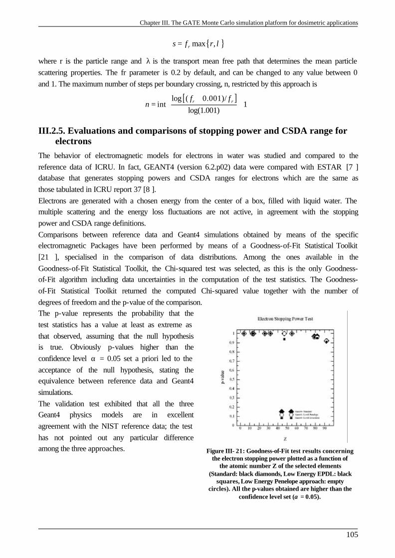
Chapter III. The GATE Monte Carlo simulation platform for dosimetric applications
105
{ }max ,rs f r λ=
where r is the particle range and λ is the transport mean free path that determines the mean particle scattering properties. The fr parameter is 0.2 by default, and can be changed to any value between 0 and 1. The maximum number of steps per boundary crossing, n, restricted by this approach is
[ ]log ( 0.001)/int 1
log(1.001)r rf f
n +
= +
III.2.5. Evaluations and comparisons of stopping power and CSDA range for electrons
The behavior of electromagnetic models for electrons in water was studied and compared to the reference data of ICRU. In fact, GEANT4 (version 6.2.p02) data were compared with ESTAR [7 ] database that generates stopping powers and CSDA ranges for electrons which are the same as those tabulated in ICRU report 37 [8 ]. Electrons are generated with a chosen energy from the center of a box, filled with liquid water. The multiple scattering and the energy loss fluctuations are not active, in agreement with the stopping power and CSDA range definitions. Comparisons between reference data and Geant4 simulations obtained by means of the specific electromagnetic Packages have been performed by means of a Goodness-of-Fit Statistical Toolkit [21 ], specialised in the comparison of data distributions. Among the ones available in the Goodness-of-Fit Statistical Toolkit, the Chi-squared test was selected, as this is the only Goodness-of-Fit algorithm including data uncertainties in the computation of the test statistics. The Goodness-of-Fit Statistical Toolkit returned the computed Chi-squared value together with the number of degrees of freedom and the p-value of the comparison. The p-value represents the probability that the test statistics has a value at least as extreme as that observed, assuming that the null hypothesis is true. Obviously p-values higher than the confidence level α = 0.05 set a priori led to the acceptance of the null hypothesis, stating the equivalence between reference data and Geant4 simulations. The validation test exhibited that all the three Geant4 physics models are in excellent agreement with the NIST reference data; the test has not pointed out any particular difference among the three approaches.
Figure III- 21: Goodness-of-Fit test results concerning the electron stopping power plotted as a function of
the atomic number Z of the selected elements (Standard: black diamonds, Low Energy EPDL: black
squares, Low Energy Penelope approach: empty circles). All the p-values obtained are higher than the
confidence level set (α = 0.05).
Chapter III. The GATE Monte Carlo simulation platform for dosimetric applications
106
III.2.6. Beta ray point source dose distributions
III.2.6.A. Introduction
Radial distributions of dose around isotropic point sources of electrons or beta emitters in an infinite water medium, or dose-point-kernels are the basis of many dosimetry problems for medical applications. This calculation is the basis for calculate doses from extended source distributions in homogeneous media or for averaging doses over finite volumes. In ocular brachytherapy, dose deposited from 106-Ru ophthalmic applicators of a given shape and of a given dimension can be derived from the calculation of dose point kernels. Analytical methods fail to account for the 3D nature of radiation transport and all relevant energy deposition processes. Monte Carlo simulations of dose point kernels is the only practical method for calculation that can consider all interactions of importance for the transport of secondary particles.
III.2.6.B. Monte Carlo calculation details
In Monte Carlo simulations, the dose around a point source is obtained by scoring the energy deposited in thin concentric spherical shells around the source per particle decay. Dose estimation techniques have been developed for photons, the linear track length kerma estimator of Williamson [22 ] that estimates the kerma by scoring tracks crossing a volume is widely used now, but there are no alternatives for electrons. In Monte Carlo calculations, the energy scored in a spherical shell delimited by the radii R1 and R2 divided by the shell mass is taken as the dose at some effective radius of the shell R1<Reff<R2. The effective radius Reff is actually the distance of a hypothetical zero thickness scoring shell from the source that would yield the same result as the finite thickness scoring shell delimited by R1 and R2 used in the calculations. The energy deposited in spherical shells has been scored to obtain dose point kernels in water for 50 keV, 100 keV, 200 keV, 1MeV and 4 MeV monoenergetic electron point sources and for 106-Rh beta sources. To model the beta sources we generated electrons following the spectrum from the ICRU Report 56 [23 ]. A cut-off of 2 keV have been chosen for the simulations. The dose distribution is converted into a dimensionless quantity as suggested by Cross [24 ] to become a slowly varying quantity with energy, making interpolation in energy more accurate with relatively wide energy intervals. This dimensionless quantity is defined as
2( / , ) 4 ( , ) /E Ej r r E r D r E r Eπρ= Equation III- 13
with r being the radial distance to the middle of the spherical shells, rE the nominal CSDA range (see Table III- 5 for the values of the CSDA range for the different electron energies, values have been taken from the NIST web database ESTAR [7 ]), ρ the density of the medium, and D(r,E) the dose per incident particle at distance r. The quantity defined in Equation III-13 represents the fraction of emitted energy that is deposited in a spherical shell of scaled radius r/rE to r/rE + d(r/rE).
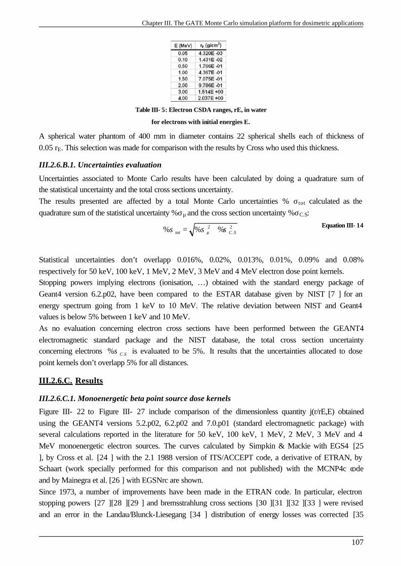
Chapter III. The GATE Monte Carlo simulation platform for dosimetric applications
107
Table III- 5: Electron CSDA ranges, rE, in water
for electrons with initial energies E.
A spherical water phantom of 400 mm in diameter contains 22 spherical shells each of thickness of 0.05 rE. This selection was made for comparison with the results by Cross who used this thickness.
III.2.6.B.1. Uncertainties evaluation
Uncertainties associated to Monte Carlo results have been calculated by doing a quadrature sum of the statistical uncertainty and the total cross sections uncertainty. The results presented are affected by a total Monte Carlo uncertainties % σtot calculated as the quadrature sum of the statistical uncertainty %σµ and the cross section uncertainty %σC.S:
2 2
.% % %tot µ C Sσ σ σ= + Equation III- 14
Statistical uncertainties don’t overlapp 0.016%, 0.02%, 0.013%, 0.01%, 0.09% and 0.08% respectively for 50 keV, 100 keV, 1 MeV, 2 MeV, 3 MeV and 4 MeV electron dose point kernels. Stopping powers implying electrons (ionisation, …) obtained with the standard energy package of Geant4 version 6.2.p02, have been compared to the ESTAR database given by NIST [7 ] for an energy spectrum going from 1 keV to 10 MeV. The relative deviation between NIST and Geant4 values is below 5% between 1 keV and 10 MeV. As no evaluation concerning electron cross sections have been performed between the GEANT4 electromagnetic standard package and the NIST database, the total cross section uncertainty concerning electrons .% C Sσ is evaluated to be 5%. It results that the uncertainties allocated to dose point kernels don’t overlapp 5% for all distances.
III.2.6.C. Results
III.2.6.C.1. Monoenergetic beta point source dose kernels
Figure III- 22 to Figure III- 27 include comparison of the dimensionless quantity j(r/rE,E) obtained using the GEANT4 versions 5.2.p02, 6.2.p02 and 7.0.p01 (standard electromagnetic package) with several calculations reported in the literature for 50 keV, 100 keV, 1 MeV, 2 MeV, 3 MeV and 4 MeV monoenergetic electron sources. The curves calculated by Simpkin & Mackie with EGS4 [25 ], by Cross et al. [24 ] with the 2.1 1988 version of ITS/ACCEPT code, a derivative of ETRAN, by Schaart (work specially performed for this comparison and not published) with the MCNP4c code and by Mainegra et al. [26 ] with EGSNrc are shown. Since 1973, a number of improvements have been made in the ETRAN code. In particular, electron stopping powers [27 ][28 ][29 ] and bremsstrahlung cross sections [30 ][31 ][32 ][33 ] were revised and an error in the Landau/Blunck-Liesegang [34 ] distribution of energy losses was corrected [35
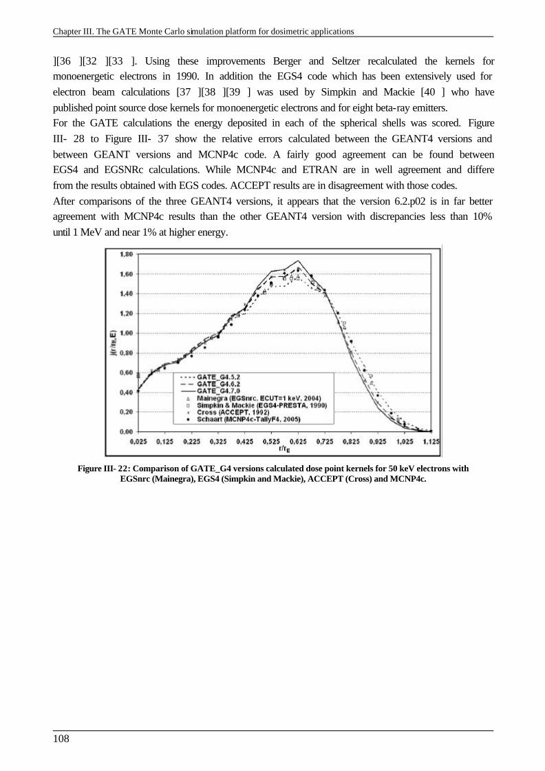
Chapter III. The GATE Monte Carlo simulation platform for dosimetric applications
108
][36 ][32 ][33 ]. Using these improvements Berger and Seltzer recalculated the kernels for monoenergetic electrons in 1990. In addition the EGS4 code which has been extensively used for electron beam calculations [37 ][38 ][39 ] was used by Simpkin and Mackie [40 ] who have published point source dose kernels for monoenergetic electrons and for eight beta-ray emitters. For the GATE calculations the energy deposited in each of the spherical shells was scored. Figure III- 28 to Figure III- 37 show the relative errors calculated between the GEANT4 versions and between GEANT versions and MCNP4c code. A fairly good agreement can be found between EGS4 and EGSNRc calculations. While MCNP4c and ETRAN are in well agreement and differe from the results obtained with EGS codes. ACCEPT results are in disagreement with those codes. After comparisons of the three GEANT4 versions, it appears that the version 6.2.p02 is in far better agreement with MCNP4c results than the other GEANT4 version with discrepancies less than 10% until 1 MeV and near 1% at higher energy.
Figure III- 22: Comparison of GATE_G4 versions calculated dose point kernels for 50 keV electrons with EGSnrc (Mainegra), EGS4 (Simpkin and Mackie), ACCEPT (Cross) and MCNP4c.
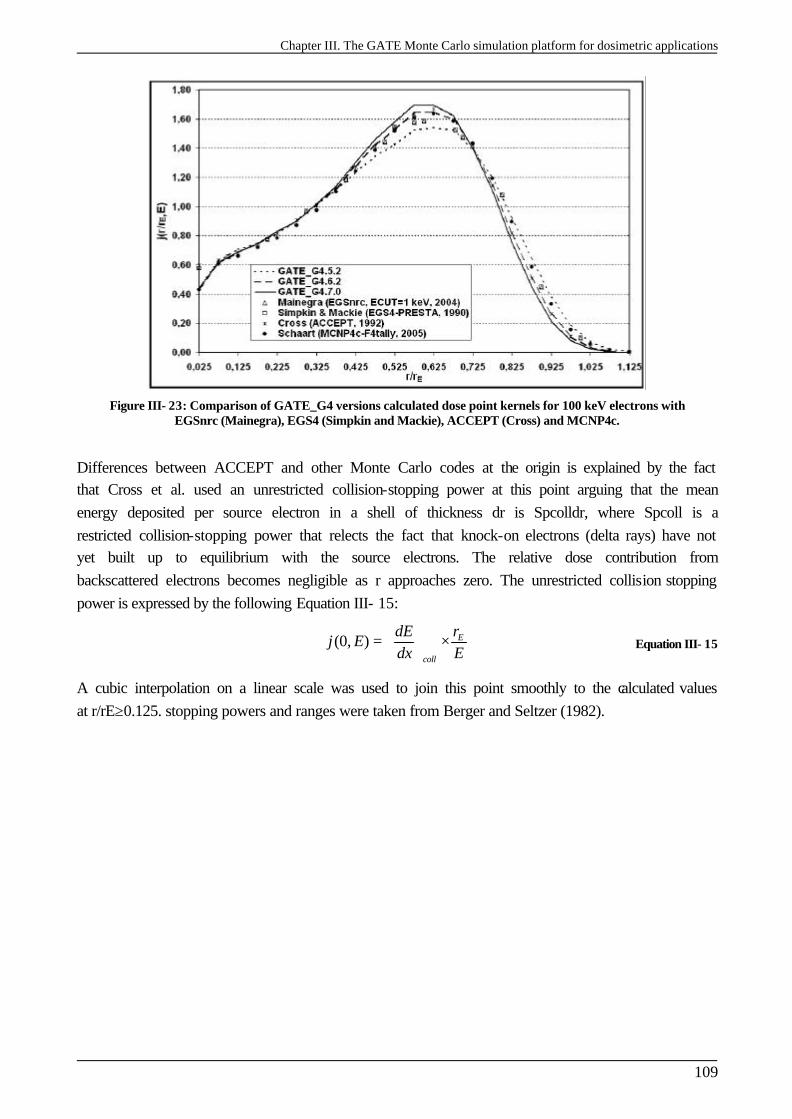
Chapter III. The GATE Monte Carlo simulation platform for dosimetric applications
109
Figure III- 23: Comparison of GATE_G4 versions calculated dose point kernels for 100 keV electrons with EGSnrc (Mainegra), EGS4 (Simpkin and Mackie), ACCEPT (Cross) and MCNP4c.
Differences between ACCEPT and other Monte Carlo codes at the origin is explained by the fact that Cross et al. used an unrestricted collision-stopping power at this point arguing that the mean energy deposited per source electron in a shell of thickness dr is Spcolldr, where Spcoll is a restricted collision-stopping power that relects the fact that knock-on electrons (delta rays) have not yet built up to equilibrium with the source electrons. The relative dose contribution from backscattered electrons becomes negligible as r approaches zero. The unrestricted collision stopping power is expressed by the following Equation III- 15:
(0, ) E
coll
rdEj E
dx E = ×
Equation III- 15
A cubic interpolation on a linear scale was used to join this point smoothly to the calculated values at r/rE≥0.125. stopping powers and ranges were taken from Berger and Seltzer (1982).
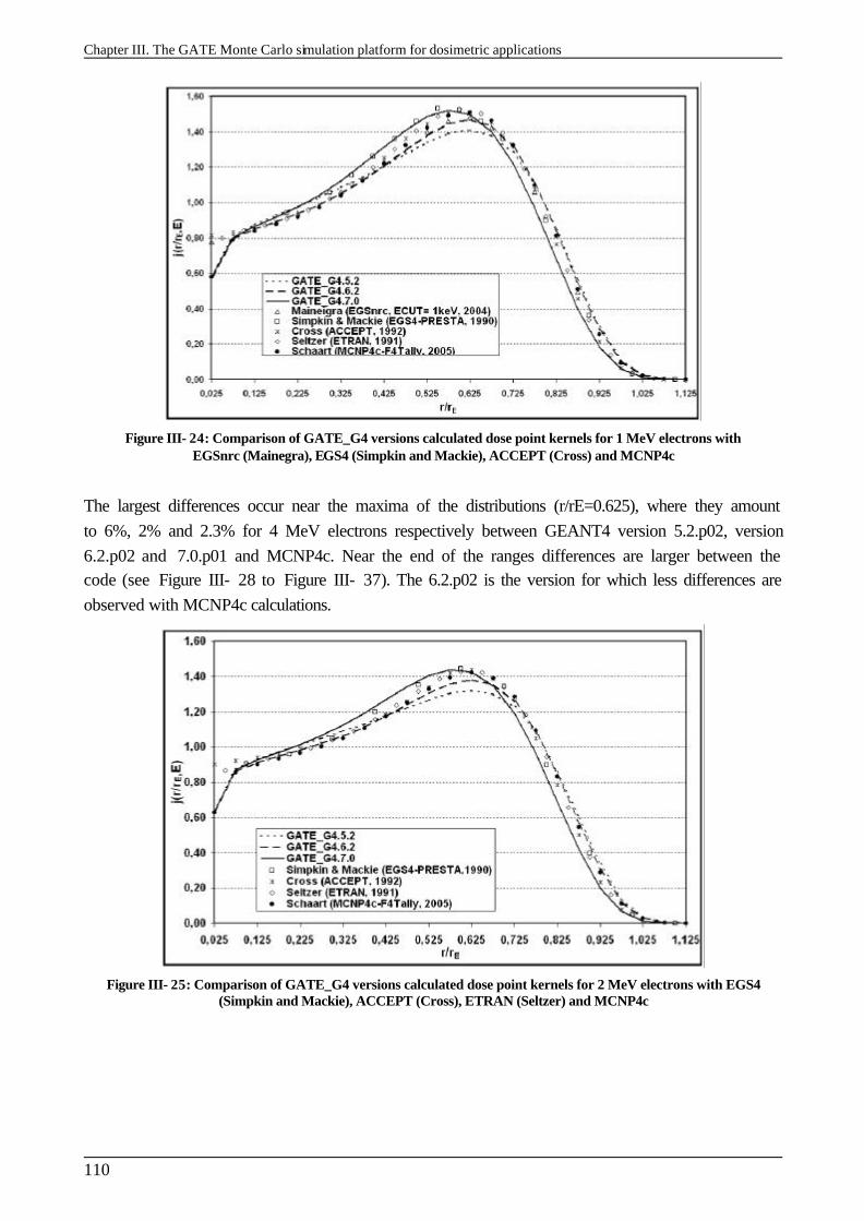
Chapter III. The GATE Monte Carlo simulation platform for dosimetric applications
110
Figure III- 24: Comparison of GATE_G4 versions calculated dose point kernels for 1 MeV electrons with EGSnrc (Mainegra), EGS4 (Simpkin and Mackie), ACCEPT (Cross) and MCNP4c
The largest differences occur near the maxima of the distributions (r/rE=0.625), where they amount to 6%, 2% and 2.3% for 4 MeV electrons respectively between GEANT4 version 5.2.p02, version 6.2.p02 and 7.0.p01 and MCNP4c. Near the end of the ranges differences are larger between the code (see Figure III- 28 to Figure III- 37). The 6.2.p02 is the version for which less differences are observed with MCNP4c calculations.
Figure III- 25: Comparison of GATE_G4 versions calculated dose point kernels for 2 MeV electrons with EGS4 (Simpkin and Mackie), ACCEPT (Cross), ETRAN (Seltzer) and MCNP4c
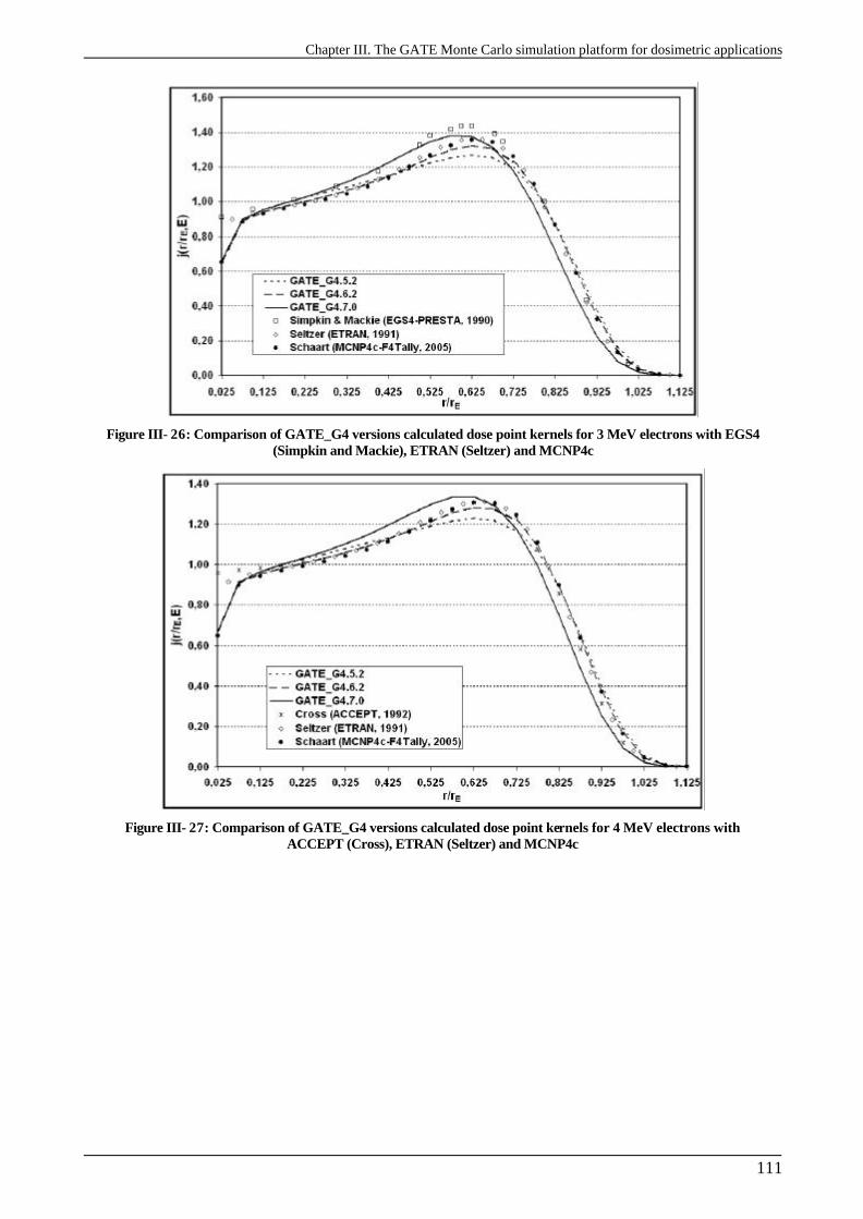
Chapter III. The GATE Monte Carlo simulation platform for dosimetric applications
111
Figure III- 26: Comparison of GATE_G4 versions calculated dose point kernels for 3 MeV electrons with EGS4 (Simpkin and Mackie), ETRAN (Seltzer) and MCNP4c
Figure III- 27: Comparison of GATE_G4 versions calculated dose point kernels for 4 MeV electrons with ACCEPT (Cross), ETRAN (Seltzer) and MCNP4c
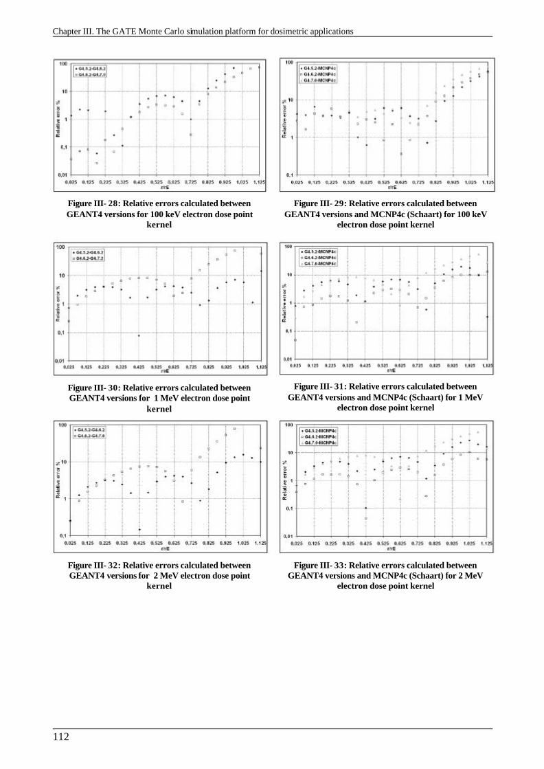
Chapter III. The GATE Monte Carlo simulation platform for dosimetric applications
112
Figure III- 28: Relative errors calculated between GEANT4 versions for 100 keV electron dose point
kernel
Figure III- 29: Relative errors calculated between GEANT4 versions and MCNP4c (Schaart) for 100 keV
electron dose point kernel
Figure III- 30: Relative errors calculated between GEANT4 versions for 1 MeV electron dose point
kernel
Figure III- 31: Relative errors calculated between GEANT4 versions and MCNP4c (Schaart) for 1 MeV
electron dose point kernel
Figure III- 32: Relative errors calculated between GEANT4 versions for 2 MeV electron dose point
kernel
Figure III- 33: Relative errors calculated between GEANT4 versions and MCNP4c (Schaart) for 2 MeV
electron dose point kernel
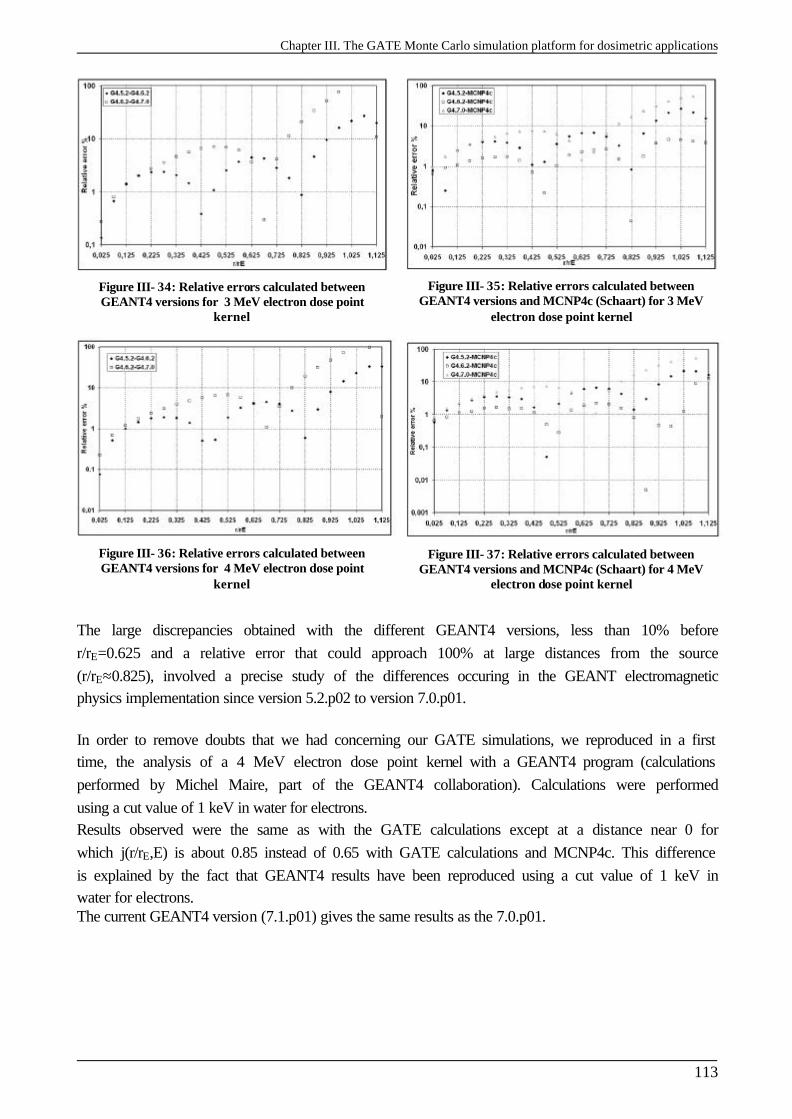
Chapter III. The GATE Monte Carlo simulation platform for dosimetric applications
113
Figure III- 34: Relative errors calculated between GEANT4 versions for 3 MeV electron dose point
kernel
Figure III- 35: Relative errors calculated between GEANT4 versions and MCNP4c (Schaart) for 3 MeV
electron dose point kernel
Figure III- 36: Relative errors calculated between GEANT4 versions for 4 MeV electron dose point
kernel
Figure III- 37: Relative errors calculated between GEANT4 versions and MCNP4c (Schaart) for 4 MeV
electron dose point kernel
The large discrepancies obtained with the different GEANT4 versions, less than 10% before r/rE=0.625 and a relative error that could approach 100% at large distances from the source (r/rE≈0.825), involved a precise study of the differences occuring in the GEANT electromagnetic physics implementation since version 5.2.p02 to version 7.0.p01. In order to remove doubts that we had concerning our GATE simulations, we reproduced in a first time, the analysis of a 4 MeV electron dose point kernel with a GEANT4 program (calculations performed by Michel Maire, part of the GEANT4 collaboration). Calculations were performed using a cut value of 1 keV in water for electrons. Results observed were the same as with the GATE calculations except at a distance near 0 for which j(r/rE,E) is about 0.85 instead of 0.65 with GATE calculations and MCNP4c. This difference is explained by the fact that GEANT4 results have been reproduced using a cut value of 1 keV in water for electrons. The current GEANT4 version (7.1.p01) gives the same results as the 7.0.p01.
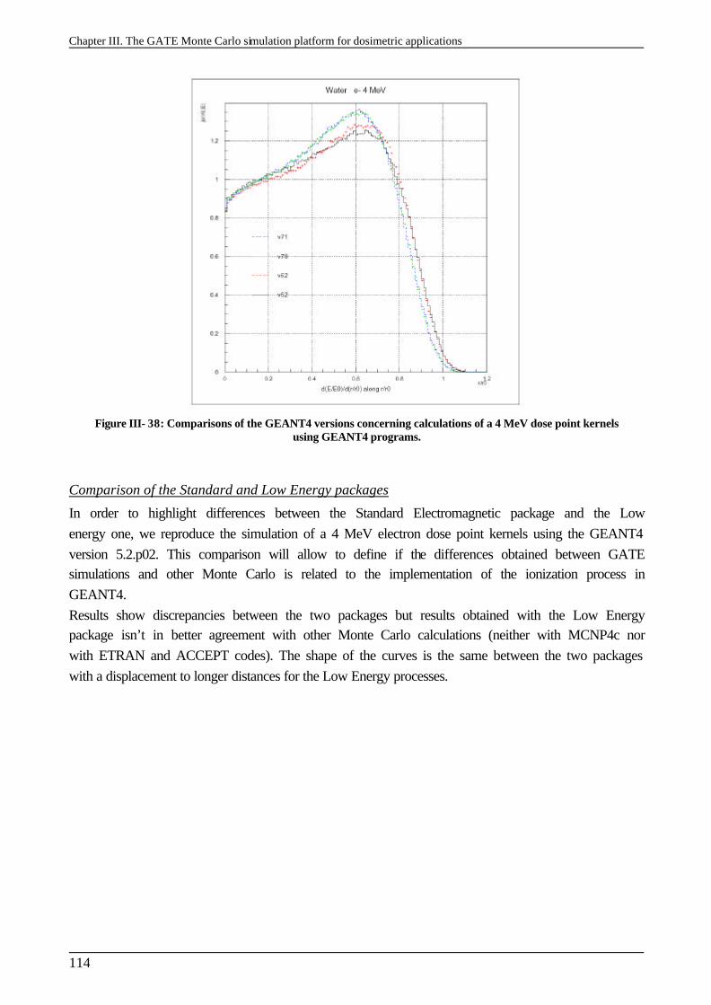
Chapter III. The GATE Monte Carlo simulation platform for dosimetric applications
114
Figure III- 38: Comparisons of the GEANT4 versions concerning calculations of a 4 MeV dose point kernels using GEANT4 programs.
Comparison of the Standard and Low Energy packages
In order to highlight differences between the Standard Electromagnetic package and the Low energy one, we reproduce the simulation of a 4 MeV electron dose point kernels using the GEANT4 version 5.2.p02. This comparison will allow to define if the differences obtained between GATE simulations and other Monte Carlo is related to the implementation of the ionization process in GEANT4. Results show discrepancies between the two packages but results obtained with the Low Energy package isn’t in better agreement with other Monte Carlo calculations (neither with MCNP4c nor with ETRAN and ACCEPT codes). The shape of the curves is the same between the two packages with a displacement to longer distances for the Low Energy processes.
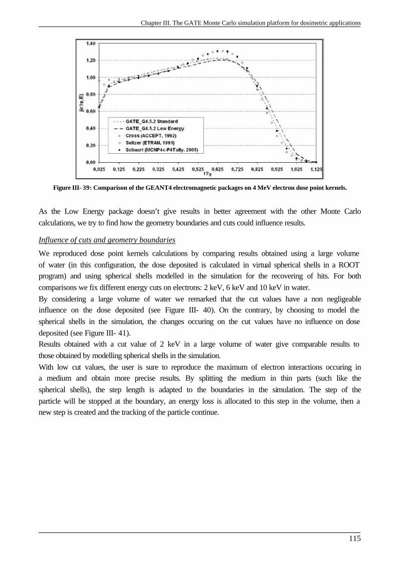
Chapter III. The GATE Monte Carlo simulation platform for dosimetric applications
115
Figure III- 39: Comparison of the GEANT4 electromagnetic packages on 4 MeV electron dose point kernels.
As the Low Energy package doesn’t give results in better agreement with the other Monte Carlo calculations, we try to find how the geometry boundaries and cuts could influence results.
Influence of cuts and geometry boundaries
We reproduced dose point kernels calculations by comparing results obtained using a large volume of water (in this configuration, the dose deposited is calculated in virtual spherical shells in a ROOT program) and using spherical shells modelled in the simulation for the recovering of hits. For both comparisons we fix different energy cuts on electrons: 2 keV, 6 keV and 10 keV in water. By considering a large volume of water we remarked that the cut values have a non negligeable influence on the dose deposited (see Figure III- 40). On the contrary, by choosing to model the spherical shells in the simulation, the changes occuring on the cut values have no influence on dose deposited (see Figure III- 41). Results obtained with a cut value of 2 keV in a large volume of water give comparable results to those obtained by modelling spherical shells in the simulation. With low cut values, the user is sure to reproduce the maximum of electron interactions occuring in a medium and obtain more precise results. By splitting the medium in thin parts (such like the spherical shells), the step length is adapted to the boundaries in the simulation. The step of the particle will be stopped at the boundary, an energy loss is allocated to this step in the volume, then a new step is created and the tracking of the particle continue.
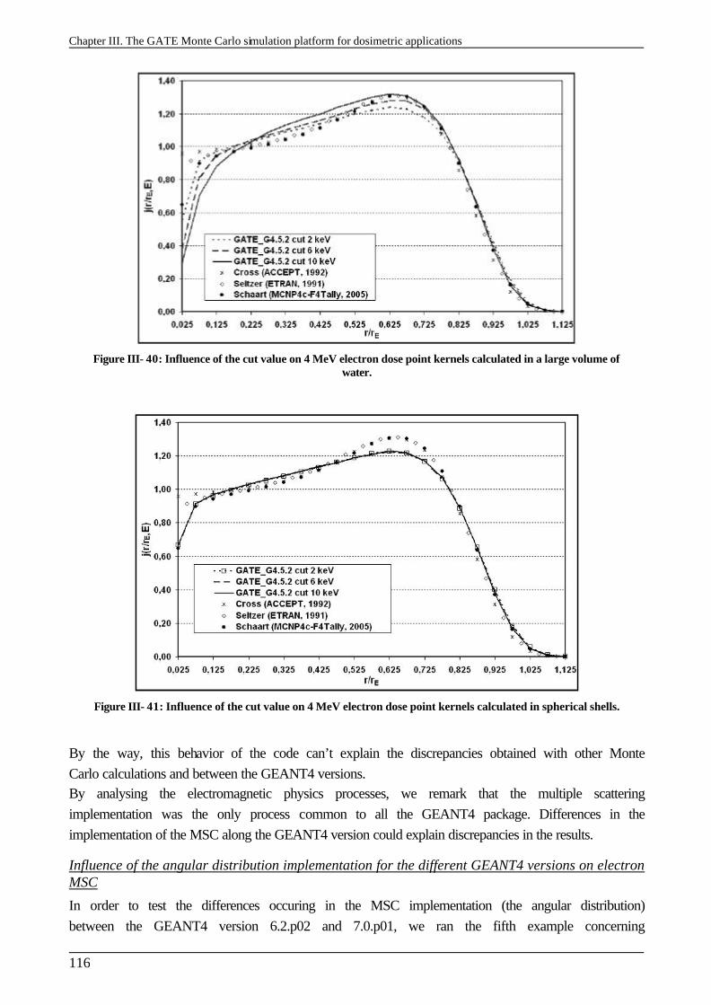
Chapter III. The GATE Monte Carlo simulation platform for dosimetric applications
116
Figure III- 40: Influence of the cut value on 4 MeV electron dose point kernels calculated in a large volume of water.
Figure III- 41: Influence of the cut value on 4 MeV electron dose point kernels calculated in spherical shells.
By the way, this behavior of the code can’t explain the discrepancies obtained with other Monte Carlo calculations and between the GEANT4 versions. By analysing the electromagnetic physics processes, we remark that the multiple scattering implementation was the only process common to all the GEANT4 package. Differences in the implementation of the MSC along the GEANT4 version could explain discrepancies in the results.
Influence of the angular distribution implementation for the different GEANT4 versions on electron MSC
In order to test the differences occuring in the MSC implementation (the angular distribution) between the GEANT4 version 6.2.p02 and 7.0.p01, we ran the fifth example concerning
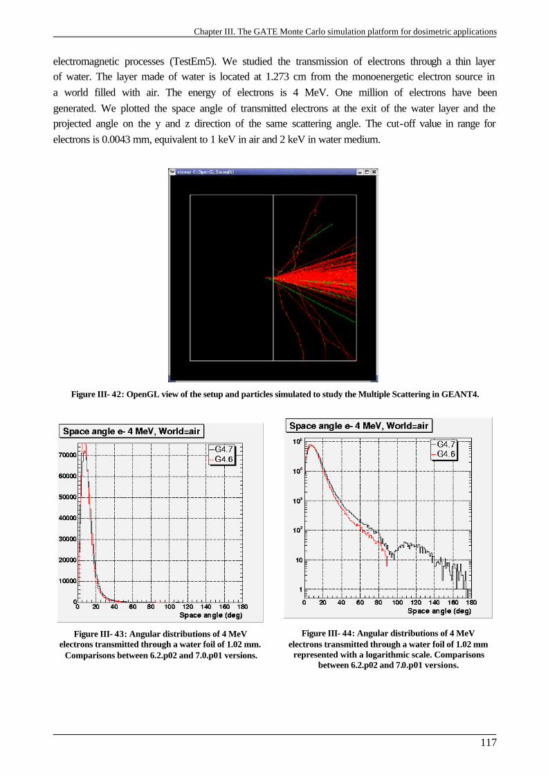
Chapter III. The GATE Monte Carlo simulation platform for dosimetric applications
117
electromagnetic processes (TestEm5). We studied the transmission of electrons through a thin layer of water. The layer made of water is located at 1.273 cm from the monoenergetic electron source in a world filled with air. The energy of electrons is 4 MeV. One million of electrons have been generated. We plotted the space angle of transmitted electrons at the exit of the water layer and the projected angle on the y and z direction of the same scattering angle. The cut-off value in range for electrons is 0.0043 mm, equivalent to 1 keV in air and 2 keV in water medium.
Figure III- 42: OpenGL view of the setup and particles simulated to study the Multiple Scattering in GEANT4.
Figure III- 43: Angular distributions of 4 MeV electrons transmitted through a water foil of 1.02 mm.
Comparisons between 6.2.p02 and 7.0.p01 versions.
Figure III- 44: Angular distributions of 4 MeV electrons transmitted through a water foil of 1.02 mm
represented with a logarithmic scale. Comparisons between 6.2.p02 and 7.0.p01 versions.
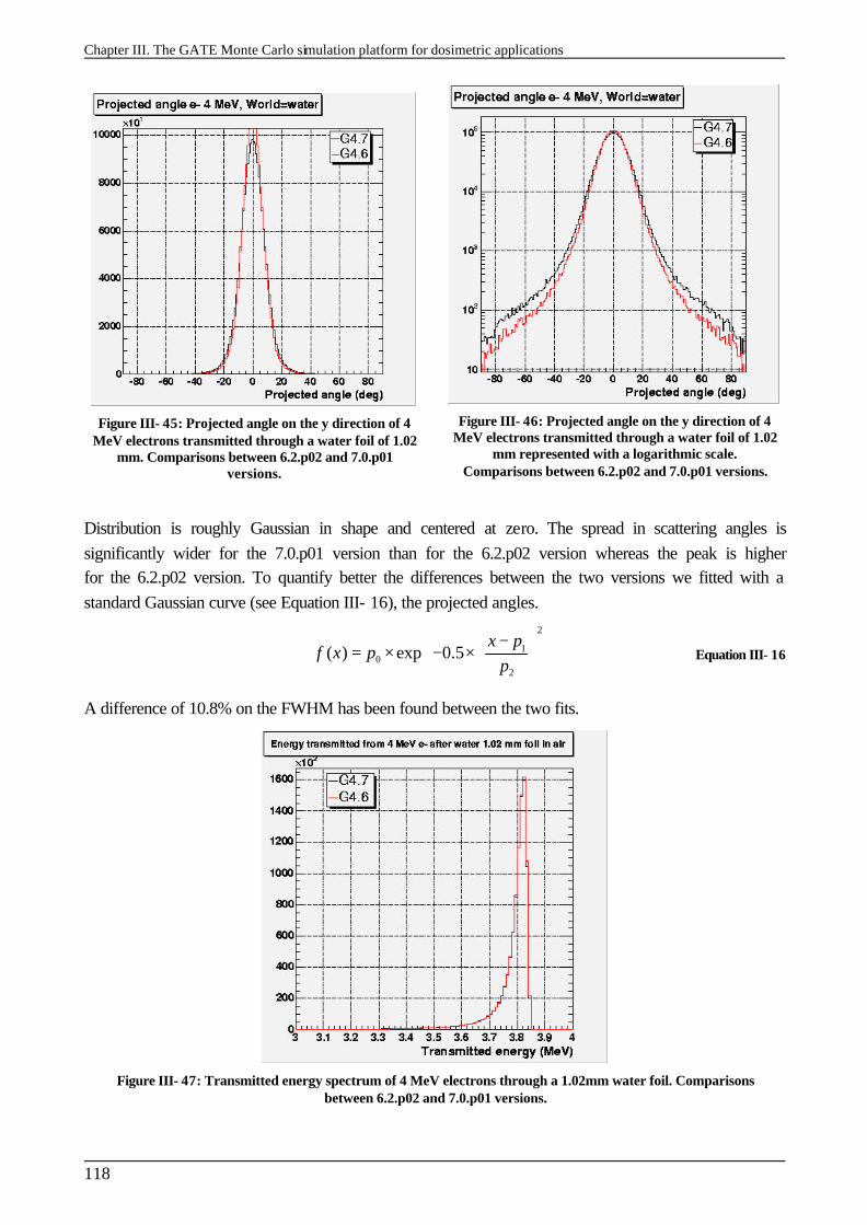
Chapter III. The GATE Monte Carlo simulation platform for dosimetric applications
118
Figure III- 45: Projected angle on the y direction of 4 MeV electrons transmitted through a water foil of 1.02
mm. Comparisons between 6.2.p02 and 7.0.p01 versions.
Figure III- 46: Projected angle on the y direction of 4 MeV electrons transmitted through a water foil of 1.02
mm represented with a logarithmic scale. Comparisons between 6.2.p02 and 7.0.p01 versions.
Distribution is roughly Gaussian in shape and centered at zero. The spread in scattering angles is significantly wider for the 7.0.p01 version than for the 6.2.p02 version whereas the peak is higher for the 6.2.p02 version. To quantify better the differences between the two versions we fitted with a standard Gaussian curve (see Equation III- 16), the projected angles.
2
10
2
( ) exp 0.5x p
f x pp
− = × − ×
Equation III- 16
A difference of 10.8% on the FWHM has been found between the two fits.
Figure III- 47: Transmitted energy spectrum of 4 MeV electrons through a 1.02mm water foil. Comparisons between 6.2.p02 and 7.0.p01 versions.
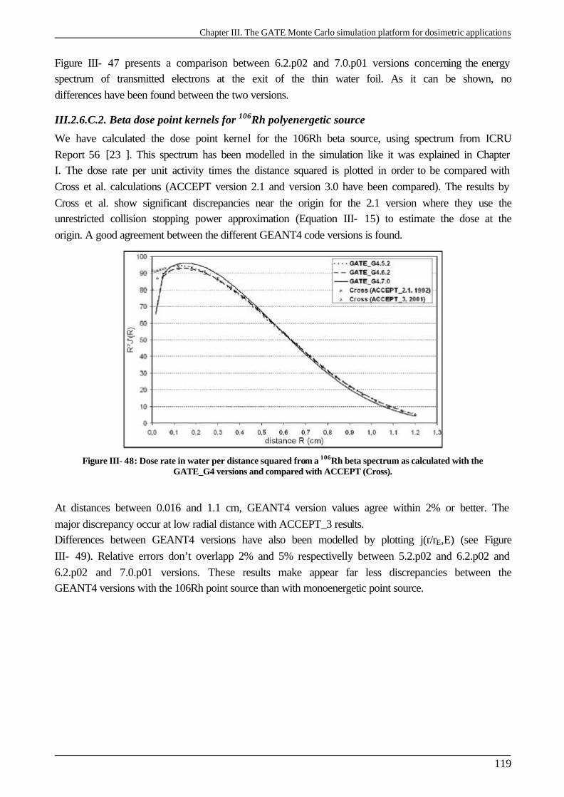
Chapter III. The GATE Monte Carlo simulation platform for dosimetric applications
119
Figure III- 47 presents a comparison between 6.2.p02 and 7.0.p01 versions concerning the energy spectrum of transmitted electrons at the exit of the thin water foil. As it can be shown, no differences have been found between the two versions.
III.2.6.C.2. Beta dose point kernels for 106Rh polyenergetic source
We have calculated the dose point kernel for the 106Rh beta source, using spectrum from ICRU Report 56 [23 ]. This spectrum has been modelled in the simulation like it was explained in Chapter I. The dose rate per unit activity times the distance squared is plotted in order to be compared with Cross et al. calculations (ACCEPT version 2.1 and version 3.0 have been compared). The results by Cross et al. show significant discrepancies near the origin for the 2.1 version where they use the unrestricted collision stopping power approximation (Equation III- 15) to estimate the dose at the origin. A good agreement between the different GEANT4 code versions is found.
Figure III- 48: Dose rate in water per distance squared from a 106Rh beta spectrum as calculated with the GATE_G4 versions and compared with ACCEPT (Cross).
At distances between 0.016 and 1.1 cm, GEANT4 version values agree within 2% or better. The major discrepancy occur at low radial distance with ACCEPT_3 results. Differences between GEANT4 versions have also been modelled by plotting j(r/rE,E) (see Figure III- 49). Relative errors don’t overlapp 2% and 5% respectivelly between 5.2.p02 and 6.2.p02 and 6.2.p02 and 7.0.p01 versions. These results make appear far less discrepancies between the GEANT4 versions with the 106Rh point source than with monoenergetic point source.
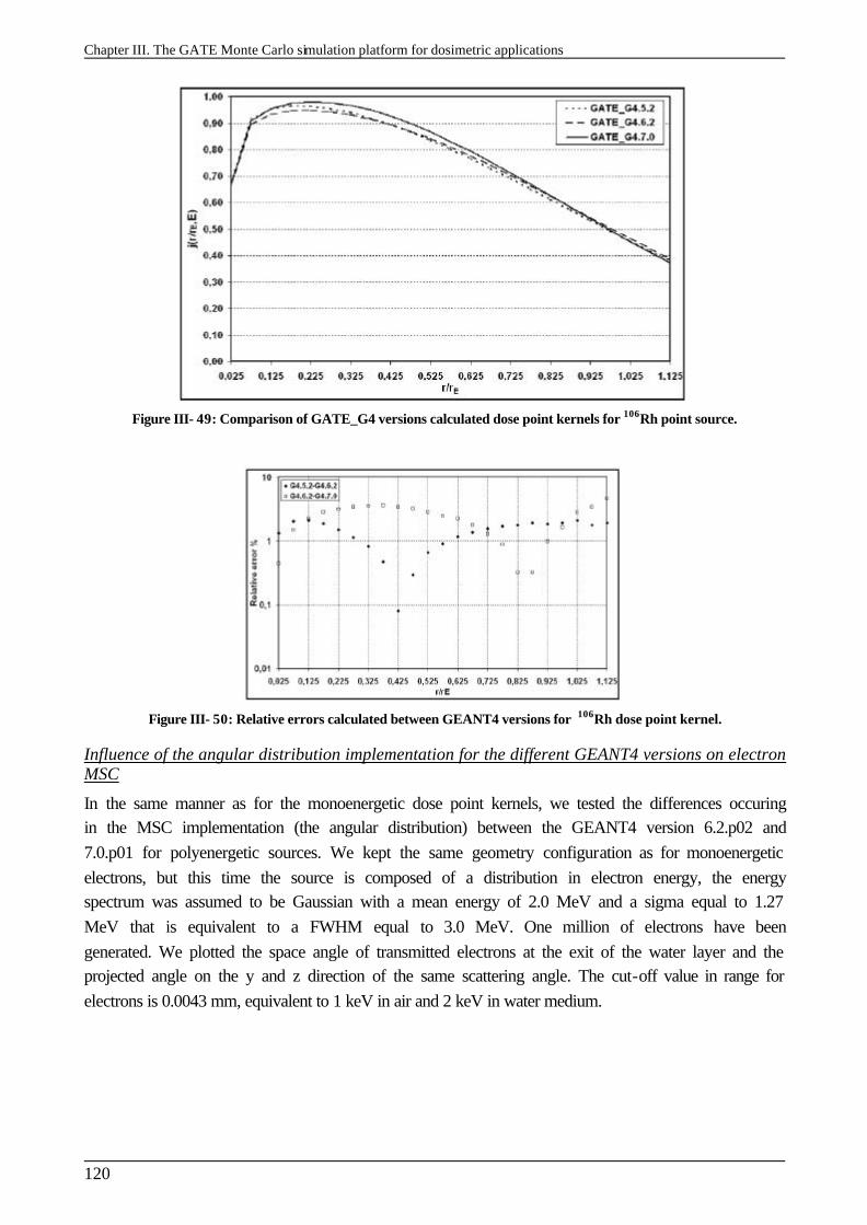
Chapter III. The GATE Monte Carlo simulation platform for dosimetric applications
120
Figure III- 49: Comparison of GATE_G4 versions calculated dose point kernels for 106Rh point source.
Figure III- 50: Relative errors calculated between GEANT4 versions for 106Rh dose point kernel.
Influence of the angular distribution implementation for the different GEANT4 versions on electron MSC
In the same manner as for the monoenergetic dose point kernels, we tested the differences occuring in the MSC implementation (the angular distribution) between the GEANT4 version 6.2.p02 and 7.0.p01 for polyenergetic sources. We kept the same geometry configuration as for monoenergetic electrons, but this time the source is composed of a distribution in electron energy, the energy spectrum was assumed to be Gaussian with a mean energy of 2.0 MeV and a sigma equal to 1.27 MeV that is equivalent to a FWHM equal to 3.0 MeV. One million of electrons have been generated. We plotted the space angle of transmitted electrons at the exit of the water layer and the projected angle on the y and z direction of the same scattering angle. The cut-off value in range for electrons is 0.0043 mm, equivalent to 1 keV in air and 2 keV in water medium.
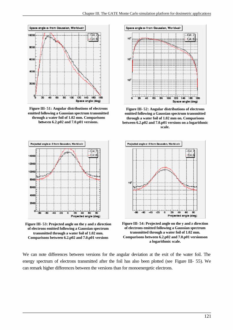
Chapter III. The GATE Monte Carlo simulation platform for dosimetric applications
121
Figure III- 51: Angular distributions of electrons emitted following a Gaussian spectrum transmitted
through a water foil of 1.02 mm. Comparisons between 6.2.p02 and 7.0.p01 versions.
Figure III- 52: Angular distributions of electrons emitted following a Gaussian spectrum transmitted through a water foil of 1.02 mm on. Comparisons
between 6.2.p02 and 7.0.p01 versions on a logarithmic scale.
Figure III- 53: Projected angle on the y and z direction of electrons emitted following a Gaussian spectrum
transmitted through a water foil of 1.02 mm. Comparisons between 6.2.p02 and 7.0.p01 versions
Figure III- 54: Projected angle on the y and z direction of electrons emitted following a Gaussian spectrum
transmitted through a water foil of 1.02 mm. Comparisons between 6.2.p02 and 7.0.p01 versionson
a logarithmic scale.
We can note differences between versions for the angular deviation at the exit of the water foil. The energy spectrum of electrons transmitted after the foil has also been plotted (see Figure III- 55). We can remark higher differences between the versions than for monoenergetic electrons.
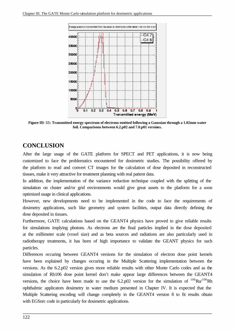
Chapter III. The GATE Monte Carlo simulation platform for dosimetric applications
122
Figure III- 55: Transmitted energy spectrum of electrons emitted following a Gaussian through a 1.02mm water foil. Comparisons between 6.2.p02 and 7.0.p01 versions.
CONCLUSION After the large usage of the GATE platform for SPECT and PET applications, it is now being customized to face the problematics encountered for dosimetric studies. The possibility offered by the platform to read and convert CT images for the calculation of dose deposited in reconstructed tissues, make it very attractive for treatment planning with real patient data. In addition, the implementation of the variance reduction technique coupled with the splitting of the simulation on cluster and/or grid environments would give great assets to the platform for a soon optimized usage in clinical applications. However, new developments need to be implemented in the code to face the requirements of dosimetry applications, such like geometry and system facilities, output data directly defining the dose deposited in tissues. Furthermore, GATE calculations based on the GEANT4 physics have proved to give reliable results for simulations implying photons. As electrons are the final particles implied in the dose deposited at the millimeter scale (voxel size) and as beta sources and radiations are also particularly used in radiotherapy treatments, it has been of high importance to validate the GEANT physics for such particles. Differences occuring between GEANT4 versions for the simulation of electron dose point kernels have been explained by changes occuring in the Multiple Scattering implementation between the versions. As the 6.2.p02 version gives more reliable results with other Monte Carlo codes and as the simulation of Rh106 dose point kernel don’t make appear large differences between the GEANT4 versions, the choice have been made to use the 6.2.p02 version for the simulation of 106Ru/106Rh ophthalmic applicators dosimetry in water medium presented in Chapter IV. It is expected that the Multiple Scattering encoding will change completely in the GEANT4 version 8 to fit results obtain with EGSnrc code in particularly for dosimetric applications.
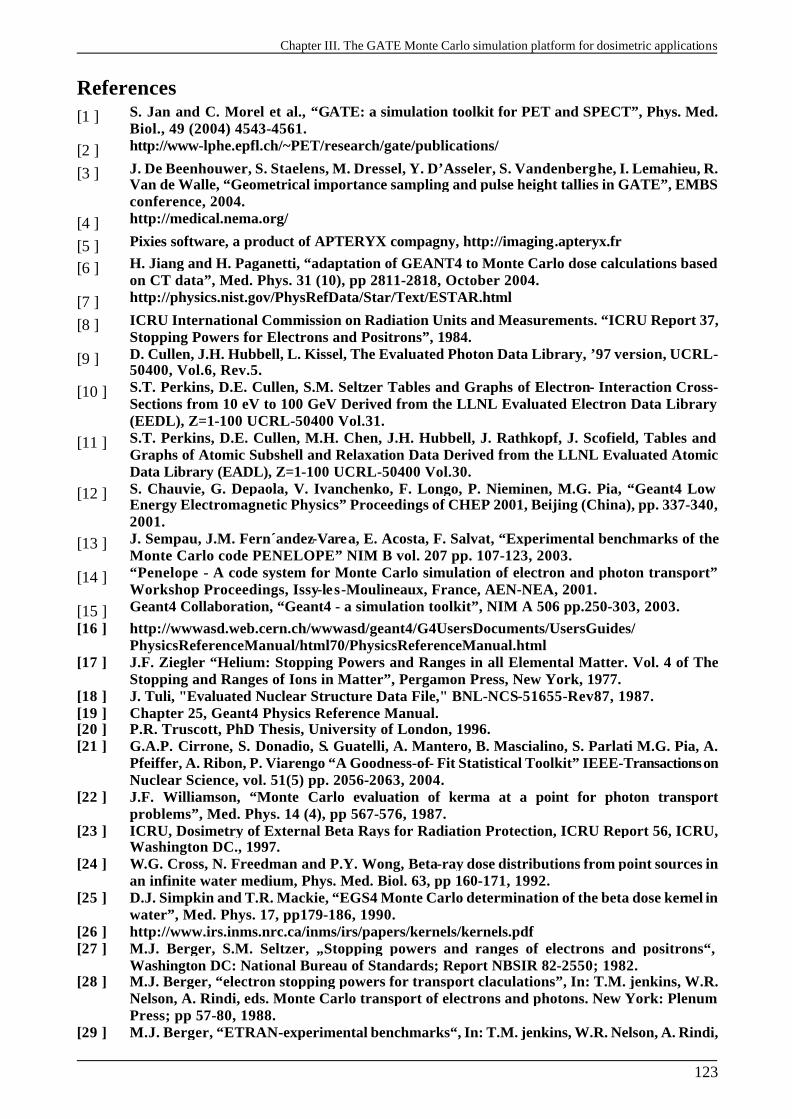
Chapter III. The GATE Monte Carlo simulation platform for dosimetric applications
123
References [1 ] S. Jan and C. Morel et al., “GATE: a simulation toolkit for PET and SPECT”, Phys. Med.
Biol., 49 (2004) 4543-4561. [2 ] http://www-lphe.epfl.ch/~PET/research/gate/publications/
[3 ] J. De Beenhouwer, S. Staelens, M. Dressel, Y. D’Asseler, S. Vandenberghe, I. Lemahieu, R. Van de Walle, “Geometrical importance sampling and pulse height tallies in GATE”, EMBS conference, 2004.
[4 ] http://medical.nema.org/
[5 ] Pixies software, a product of APTERYX compagny, http://imaging.apteryx.fr
[6 ] H. Jiang and H. Paganetti, “adaptation of GEANT4 to Monte Carlo dose calculations based on CT data”, Med. Phys. 31 (10), pp 2811-2818, October 2004.
[7 ] http://physics.nist.gov/PhysRefData/Star/Text/ESTAR.html
[8 ] ICRU International Commission on Radiation Units and Measurements. “ICRU Report 37, Stopping Powers for Electrons and Positrons”, 1984.
[9 ] D. Cullen, J.H. Hubbell, L. Kissel, The Evaluated Photon Data Library, ’97 version, UCRL-50400, Vol.6, Rev.5.
[10 ] S.T. Perkins, D.E. Cullen, S.M. Seltzer Tables and Graphs of Electron- Interaction Cross-Sections from 10 eV to 100 GeV Derived from the LLNL Evaluated Electron Data Library (EEDL), Z=1-100 UCRL-50400 Vol.31.
[11 ] S.T. Perkins, D.E. Cullen, M.H. Chen, J.H. Hubbell, J. Rathkopf, J. Scofield, Tables and Graphs of Atomic Subshell and Relaxation Data Derived from the LLNL Evaluated Atomic Data Library (EADL), Z=1-100 UCRL-50400 Vol.30.
[12 ] S. Chauvie, G. Depaola, V. Ivanchenko, F. Longo, P. Nieminen, M.G. Pia, “Geant4 Low Energy Electromagnetic Physics” Proceedings of CHEP 2001, Beijing (China), pp. 337-340, 2001.
[13 ] J. Sempau, J.M. Fern´andez-Varea, E. Acosta, F. Salvat, “Experimental benchmarks of the Monte Carlo code PENELOPE” NIM B vol. 207 pp. 107-123, 2003.
[14 ] “Penelope - A code system for Monte Carlo simulation of electron and photon transport” Workshop Proceedings, Issy-les-Moulineaux, France, AEN-NEA, 2001.
[15 ] Geant4 Collaboration, “Geant4 - a simulation toolkit”, NIM A 506 pp.250-303, 2003. [16 ] http://wwwasd.web.cern.ch/wwwasd/geant4/G4UsersDocuments/UsersGuides/
PhysicsReferenceManual/html70/PhysicsReferenceManual.html [17 ] J.F. Ziegler “Helium: Stopping Powers and Ranges in all Elemental Matter. Vol. 4 of The
Stopping and Ranges of Ions in Matter”, Pergamon Press, New York, 1977. [18 ] J. Tuli, "Evaluated Nuclear Structure Data File," BNL-NCS-51655-Rev87, 1987. [19 ] Chapter 25, Geant4 Physics Reference Manual. [20 ] P.R. Truscott, PhD Thesis, University of London, 1996. [21 ] G.A.P. Cirrone, S. Donadio, S. Guatelli, A. Mantero, B. Mascialino, S. Parlati M.G. Pia, A.
Pfeiffer, A. Ribon, P. Viarengo “A Goodness-of- Fit Statistical Toolkit” IEEE-Transactions on Nuclear Science, vol. 51(5) pp. 2056-2063, 2004.
[22 ] J.F. Williamson, “Monte Carlo evaluation of kerma at a point for photon transport problems”, Med. Phys. 14 (4), pp 567-576, 1987.
[23 ] ICRU, Dosimetry of External Beta Rays for Radiation Protection, ICRU Report 56, ICRU, Washington DC., 1997.
[24 ] W.G. Cross, N. Freedman and P.Y. Wong, Beta-ray dose distributions from point sources in an infinite water medium, Phys. Med. Biol. 63, pp 160-171, 1992.
[25 ] D.J. Simpkin and T.R. Mackie, “EGS4 Monte Carlo determination of the beta dose kernel in water”, Med. Phys. 17, pp179-186, 1990.
[26 ] http://www.irs.inms.nrc.ca/inms/irs/papers/kernels/kernels.pdf [27 ] M.J. Berger, S.M. Seltzer, „Stopping powers and ranges of electrons and positrons“,
Washington DC: National Bureau of Standards; Report NBSIR 82-2550; 1982. [28 ] M.J. Berger, “electron stopping powers for transport claculations”, In: T.M. jenkins, W.R.
Nelson, A. Rindi, eds. Monte Carlo transport of electrons and photons. New York: Plenum Press; pp 57-80, 1988.
[29 ] M.J. Berger, “ETRAN-experimental benchmarks“, In: T.M. jenkins, W.R. Nelson, A. Rindi, eds. Monte Carlo transport of electrons and photons. New York: Plenum Press; pp 57-80,
Chapter III. The GATE Monte Carlo simulation platform for dosimetric applications
124
eds. Monte Carlo transport of electrons and photons. New York: Plenum Press; pp 57-80, 1988.
[30 ] S.M. Seltzer, M.J. Berger, “Bremsstrahlung spectra from electron interactions with screened atomic nuclei and orbital electrons”, Nucl. Instrum. Meth. B12:95-134, 1985.
[31 ] S.M. Seltzer, M.J. Berger, “Bremsstrahlung energy spectra from electrons with kinetic energy 1 keV-10 GeV incident on screened nuclei and orbital electrons of neutral atoms with Z=1-100. At. Data and Nucl. Data Tables 35:345-418; 1986.
[32 ] S.M. Seltzer, M.J. Berger, „Cross sections for bremsstrahlung production and electron impact ionization”, In: T.M. jenkins, W.R. Nelson, A. Rindi, eds. Monte Carlo transport of electrons and photons. New York: Plenum Press;pp 323-344, 1988.
[33 ] S.M. Seltzer, M.J. Berger, “An overview of ETRAN Monte Carlo methods”, In: T.M. jenkins, W.R. Nelson, A. Rindi, eds. Monte Carlo transport of electrons and photons. New York: Plenum Press;pp 81-114, 1988.
[34 ] O. Blunck, S. Liesegang, “On the energy loss of fast electrons in thin films”, Z. für Phys. 128:500-505; 1950 (in German).
[35 ] J.A. Halbleib, “Structure and operation of the ITS code system”, In: T.M. jenkins, W.R. Nelson, A. Rindi, eds. Monte Carlo transport of electrons and photons. New York: Plenum Press;pp 249-262, 1988.
[36 ] J.A. Halbleib, “Applications of the ITS code”, In: T.M. jenkins, W.R. Nelson, A. Rindi, eds. Monte Carlo transport of electrons and photons. New York: Plenum Press;pp 263-286, 1988.
[37 ] D.W.O. Rogers, “Fluence to dose equivalent conversion factors calculated with EGS3 for electrons from 100 keV to 20 GeV and photons from 11 keV to 20 GeV. Health Phys. 45:891-914, 1984.
[38 ] D.W.O Rogers, A.F. Bielajew, “Differences in electron depth dose curves calculated with EGS and ETRAN and improved energy range relationships”, Med. Phys. 13:687-694, 1986.
[39 ] A.F. Bielajew, D.W.O. Rogers, “Presta: the parameter reduced electron-step transport algorithm for electron Monte Carlo transport”, Nucl. Inst. Methods B18:165-181, 1987.
[40 ] D.J. Simpkin, T.R. Mackie, “EGS4 Monte Carlo determination of the beta dose kernel in water”, Med. Phys. 17:179-186, 1990.
Chapter IV. 106Ru/106Rh ocular brachytherapy treatment planning using GATE. Preliminary studies using CT images.
125
Chapter IV. 106Ru/106Rh ocular brachytherapy treatment planning using GATE. Preliminary studies using CT images. INTRODUCTION The integration of point kernels is used in some hospitals and laboratories for calculating dose in the eye and elsewhere. In Centre Jean Perrin the analytic software Plaque Simulator (version 5.3.2) uses a cruder method that consists into summing over some hundreds of individual point sources to estimate the dose rates in a modelled eye. The goal is to quantify how accurately eye applicator doses can be calculated by different methods using Monte Carlo, integration of point kernels or analytic calculations. We compare in a first part our GATE Monte Carlo results using the GEANT4 version 6.2.p02 with measurements and the previous cited three calculation methods. Doses are calculated in water on the central axis and on the median plan of the beta emitter ophthalmic applicators. After a validation in aqueous media, the ambition is to use GATE Monte Carlo platform on voxellized images described by CT slices. In order to perform such treatment planning with GATE, in a second part, we study the impact of the translation of CT numbers on tissue parameters (density and atomic composition of human tissues) on the dose deposited by photon and electron beams. Soft and bone tissues described by a gray scale in CT slices are identified to be well translated by colouring the corresponded Hounsfield units in voxels using the tool in Chapter IV. Then, the influence of the translation of tissue parameters on the dose deposited by electron and photon beams is studied.

Chapter IV. 106Ru/106Rh ocular brachytherapy treatment planning using GATE. Preliminary studies using CT images.
126
IV.1. 106Ru/106Rh OCULAR BRACHYTHERAPY TREATMENT PLANNING USING GATE
IV.1.1. Theoretical calculation of the beta point source dose function for 106Ru/106Rh eye applicators, comparisons
The beta point kernels for radionuclides can be obtained from theoretical calculations. Loevinger [1 ] proposed in 1956, a function describing the β emission of radionuclides based on the data available at that time. Two types of measurement can be performed. First, the measurements can be performed using extrapolation chambers on extended plane sources; an homogeneous medium and dimensions of the beta plane source larger than the diameter of the chamber have been chosen for a reliable measurement. A second method is to measure the dose distribution around a point source of a β-emitting radionuclide in air (isodoses in air are sufficiently extended to allow the usage of large size detectors). The air must be free and the scattering produced by objects must be negligible. Then, dose distributions in tissue are derived from dose distributions in air by applying corrections concerning the differences in medium composition and density [2 ][3 ]. From these types of measurements, the beta point source dose function can be derived using mathematics. By taking into account more recent experimental data (those of Cross in 1967) [4 ], and the theoretical studies of Berger [3 ][5 ], a new function has been established.
IV.1.1.A. The function of Loevinger
IV.1.1.A.1. Definition
The function proposed by Loevinger is the following:
2( ) 1 exp 1 exp(1 )( )
BJ c
c cρυξ ρυξ
ξ ρυξ ρυξρυξ
= − − + × − Equation IV-1
[ ] 0with for cρυξ≡ ≥ where J(ξ) is the absorbed dose rate at a distance ξ (in cm) from the point source (in Gy MBq-1h-1) υ is an apparent absorption coefficient (in cm2 g-1) ρ is the density of the homogeneous medium (in g cm-3) c is a dimensionless parameter, which gives the value of the first term inside the curly bracket at ξ = 0 and also the value ρυξ at which this term becomes and remains zero, B is a normalising constant, evaluated by the requirement that the total energy absorbed in avery large sphere must just be the energy emitted.
( ) ( )2 3
22 31 1 3 2 1
4.60 10EB
GyMBq h MeVgcm cm g
βρ υα
−
−− − − −
= × Equation IV-2
with 1 2 23 ( 1)c c eα − = − − To match accurately the Berger and Cross data, the following expression has been proposed by Vynckier and Wambersie [6 ]:
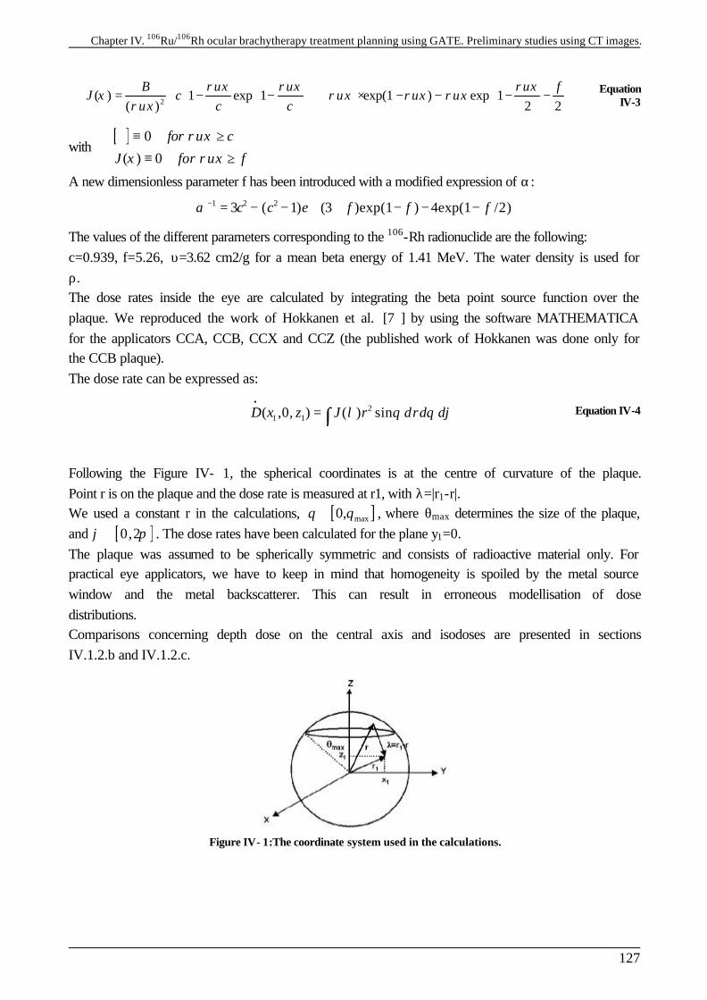
Chapter IV. 106Ru/106Rh ocular brachytherapy treatment planning using GATE. Preliminary studies using CT images.
127
2( ) 1 exp 1 exp(1 ) exp 1
( ) 2 2B f
J cc c
ρυξ ρυξ ρυξξ ρυξ ρυξ ρυξ
ρυξ = − − + × − − − −
Equation IV-3
with [ ] 0
( ) 0
for c
J for f
ρυξ
ξ ρυξ
≡ ≥
≡ ≥
A new dimensionless parameter f has been introduced with a modified expression of α: 1 2 23 ( 1) (3 )exp(1 ) 4exp(1 /2)c c e f f fα − = − − + + − − −
The values of the different parameters corresponding to the 106-Rh radionuclide are the following: c=0.939, f=5.26, υ=3.62 cm2/g for a mean beta energy of 1.41 MeV. The water density is used for ρ. The dose rates inside the eye are calculated by integrating the beta point source function over the plaque. We reproduced the work of Hokkanen et al. [7 ] by using the software MATHEMATICA for the applicators CCA, CCB, CCX and CCZ (the published work of Hokkanen was done only for the CCB plaque). The dose rate can be expressed as:
2
1 1( ,0, ) ( ) sinD x z J r drd dλ θ θ ϕ•
= ∫ Equation IV-4
Following the Figure IV- 1, the spherical coordinates is at the centre of curvature of the plaque. Point r is on the plaque and the dose rate is measured at r1, with λ=|r1-r|. We used a constant r in the calculations, [ ]max0,θ θ∈ , where θmax determines the size of the plaque, and [ ]0,2ϕ π∈ . The dose rates have been calculated for the plane y1=0. The plaque was assumed to be spherically symmetric and consists of radioactive material only. For practical eye applicators, we have to keep in mind that homogeneity is spoiled by the metal source window and the metal backscatterer. This can result in erroneous modellisation of dose distributions. Comparisons concerning depth dose on the central axis and isodoses are presented in sections IV.1.2.b and IV.1.2.c.
Figure IV- 1:The coordinate system used in the calculations.
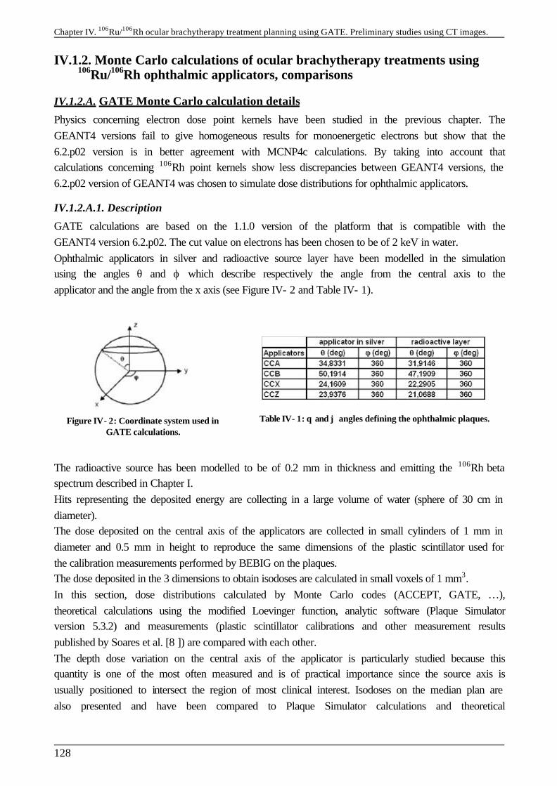
Chapter IV. 106Ru/106Rh ocular brachytherapy treatment planning using GATE. Preliminary studies using CT images.
128
IV.1.2. Monte Carlo calculations of ocular brachytherapy treatments using 106Ru/106Rh ophthalmic applicators, comparisons
IV.1.2.A. GATE Monte Carlo calculation details
Physics concerning electron dose point kernels have been studied in the previous chapter. The GEANT4 versions fail to give homogeneous results for monoenergetic electrons but show that the 6.2.p02 version is in better agreement with MCNP4c calculations. By taking into account that calculations concerning 106Rh point kernels show less discrepancies between GEANT4 versions, the 6.2.p02 version of GEANT4 was chosen to simulate dose distributions for ophthalmic applicators.
IV.1.2.A.1. Description
GATE calculations are based on the 1.1.0 version of the platform that is compatible with the GEANT4 version 6.2.p02. The cut value on electrons has been chosen to be of 2 keV in water. Ophthalmic applicators in silver and radioactive source layer have been modelled in the simulation using the angles θ and ϕ which describe respectively the angle from the central axis to the applicator and the angle from the x axis (see Figure IV- 2 and Table IV- 1).
Figure IV- 2: Coordinate system used in GATE calculations.
Table IV- 1: θ and ϕ angles defining the ophthalmic plaques.
The radioactive source has been modelled to be of 0.2 mm in thickness and emitting the 106Rh beta spectrum described in Chapter I. Hits representing the deposited energy are collecting in a large volume of water (sphere of 30 cm in diameter). The dose deposited on the central axis of the applicators are collected in small cylinders of 1 mm in diameter and 0.5 mm in height to reproduce the same dimensions of the plastic scintillator used for the calibration measurements performed by BEBIG on the plaques. The dose deposited in the 3 dimensions to obtain isodoses are calculated in small voxels of 1 mm3. In this section, dose distributions calculated by Monte Carlo codes (ACCEPT, GATE, …), theoretical calculations using the modified Loevinger function, analytic software (Plaque Simulator version 5.3.2) and measurements (plastic scintillator calibrations and other measurement results published by Soares et al. [8 ]) are compared with each other. The depth dose variation on the central axis of the applicator is particularly studied because this quantity is one of the most often measured and is of practical importance since the source axis is usually positioned to intersect the region of most clinical interest. Isodoses on the median plan are also presented and have been compared to Plaque Simulator calculations and theoretical
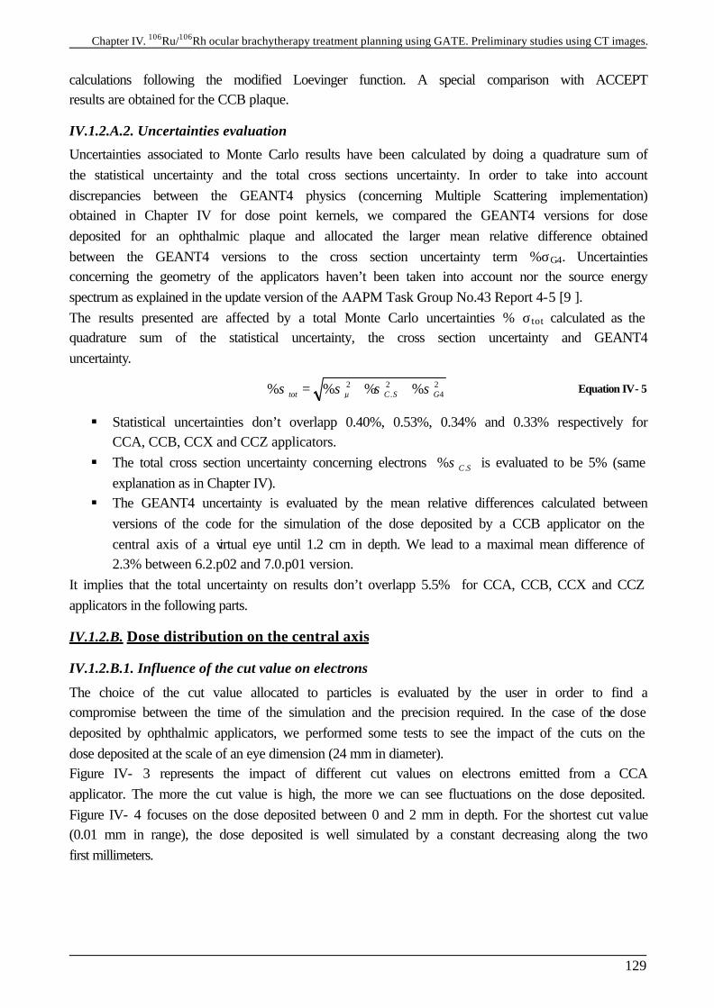
Chapter IV. 106Ru/106Rh ocular brachytherapy treatment planning using GATE. Preliminary studies using CT images.
129
calculations following the modified Loevinger function. A special comparison with ACCEPT results are obtained for the CCB plaque.
IV.1.2.A.2. Uncertainties evaluation
Uncertainties associated to Monte Carlo results have been calculated by doing a quadrature sum of the statistical uncertainty and the total cross sections uncertainty. In order to take into account discrepancies between the GEANT4 physics (concerning Multiple Scattering implementation) obtained in Chapter IV for dose point kernels, we compared the GEANT4 versions for dose deposited for an ophthalmic plaque and allocated the larger mean relative difference obtained between the GEANT4 versions to the cross section uncertainty term %σG4. Uncertainties concerning the geometry of the applicators haven’t been taken into account nor the source energy spectrum as explained in the update version of the AAPM Task Group No.43 Report 4-5 [9 ]. The results presented are affected by a total Monte Carlo uncertainties % σtot calculated as the quadrature sum of the statistical uncertainty, the cross section uncertainty and GEANT4 uncertainty.
2 2 2
. 4% % % %tot µ C S Gσ σ σ σ= + + Equation IV- 5
§ Statistical uncertainties don’t overlapp 0.40%, 0.53%, 0.34% and 0.33% respectively for CCA, CCB, CCX and CCZ applicators.
§ The total cross section uncertainty concerning electrons .% C Sσ is evaluated to be 5% (same explanation as in Chapter IV).
§ The GEANT4 uncertainty is evaluated by the mean relative differences calculated between versions of the code for the simulation of the dose deposited by a CCB applicator on the central axis of a virtual eye until 1.2 cm in depth. We lead to a maximal mean difference of 2.3% between 6.2.p02 and 7.0.p01 version.
It implies that the total uncertainty on results don’t overlapp 5.5% for CCA, CCB, CCX and CCZ applicators in the following parts.
IV.1.2.B. Dose distribution on the central axis
IV.1.2.B.1. Influence of the cut value on electrons
The choice of the cut value allocated to particles is evaluated by the user in order to find a compromise between the time of the simulation and the precision required. In the case of the dose deposited by ophthalmic applicators, we performed some tests to see the impact of the cuts on the dose deposited at the scale of an eye dimension (24 mm in diameter). Figure IV- 3 represents the impact of different cut values on electrons emitted from a CCA applicator. The more the cut value is high, the more we can see fluctuations on the dose deposited. Figure IV- 4 focuses on the dose deposited between 0 and 2 mm in depth. For the shortest cut value (0.01 mm in range), the dose deposited is well simulated by a constant decreasing along the two first millimeters.
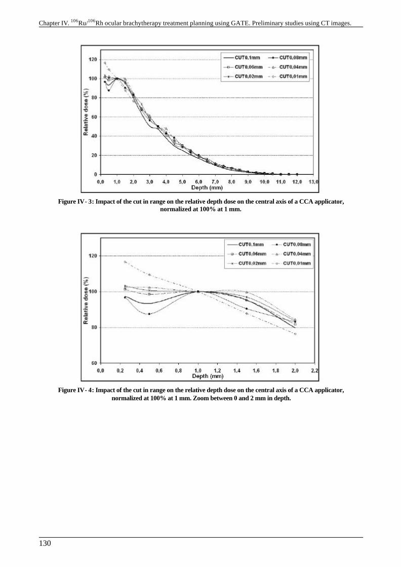
Chapter IV. 106Ru/106Rh ocular brachytherapy treatment planning using GATE. Preliminary studies using CT images.
130
Figure IV- 3: Impact of the cut in range on the relative depth dose on the central axis of a CCA applicator, normalized at 100% at 1 mm.
Figure IV- 4: Impact of the cut in range on the relative depth dose on the central axis of a CCA applicator, normalized at 100% at 1 mm. Zoom between 0 and 2 mm in depth.
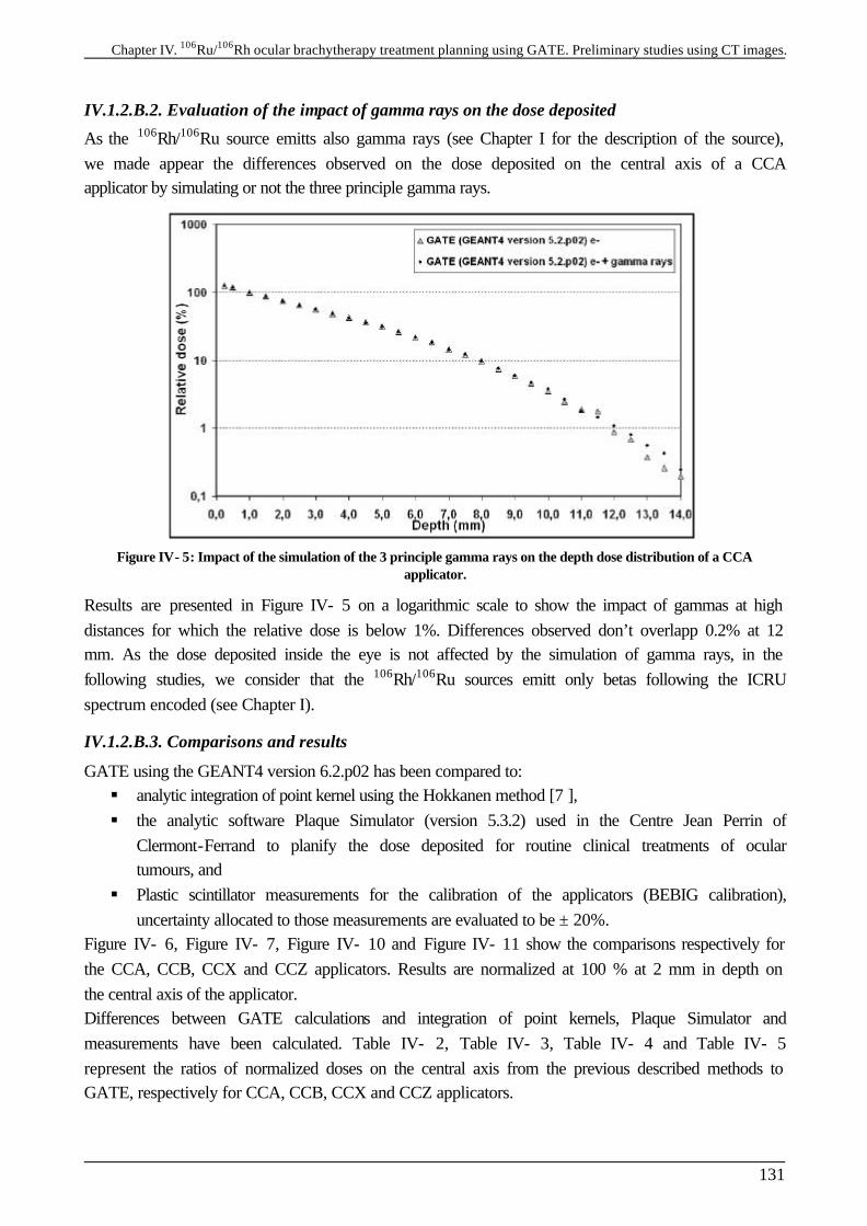
Chapter IV. 106Ru/106Rh ocular brachytherapy treatment planning using GATE. Preliminary studies using CT images.
131
IV.1.2.B.2. Evaluation of the impact of gamma rays on the dose deposited
As the 106Rh/106Ru source emitts also gamma rays (see Chapter I for the description of the source), we made appear the differences observed on the dose deposited on the central axis of a CCA applicator by simulating or not the three principle gamma rays.
Figure IV- 5: Impact of the simulation of the 3 principle gamma rays on the depth dose distribution of a CCA applicator.
Results are presented in Figure IV- 5 on a logarithmic scale to show the impact of gammas at high distances for which the relative dose is below 1%. Differences observed don’t overlapp 0.2% at 12 mm. As the dose deposited inside the eye is not affected by the simulation of gamma rays, in the following studies, we consider that the 106Rh/106Ru sources emitt only betas following the ICRU spectrum encoded (see Chapter I).
IV.1.2.B.3. Comparisons and results
GATE using the GEANT4 version 6.2.p02 has been compared to: § analytic integration of point kernel using the Hokkanen method [7 ], § the analytic software Plaque Simulator (version 5.3.2) used in the Centre Jean Perrin of
Clermont-Ferrand to planify the dose deposited for routine clinical treatments of ocular tumours, and
§ Plastic scintillator measurements for the calibration of the applicators (BEBIG calibration), uncertainty allocated to those measurements are evaluated to be ± 20%.
Figure IV- 6, Figure IV- 7, Figure IV- 10 and Figure IV- 11 show the comparisons respectively for the CCA, CCB, CCX and CCZ applicators. Results are normalized at 100 % at 2 mm in depth on the central axis of the applicator. Differences between GATE calculations and integration of point kernels, Plaque Simulator and measurements have been calculated. Table IV- 2, Table IV- 3, Table IV- 4 and Table IV- 5 represent the ratios of normalized doses on the central axis from the previous described methods to GATE, respectively for CCA, CCB, CCX and CCZ applicators.
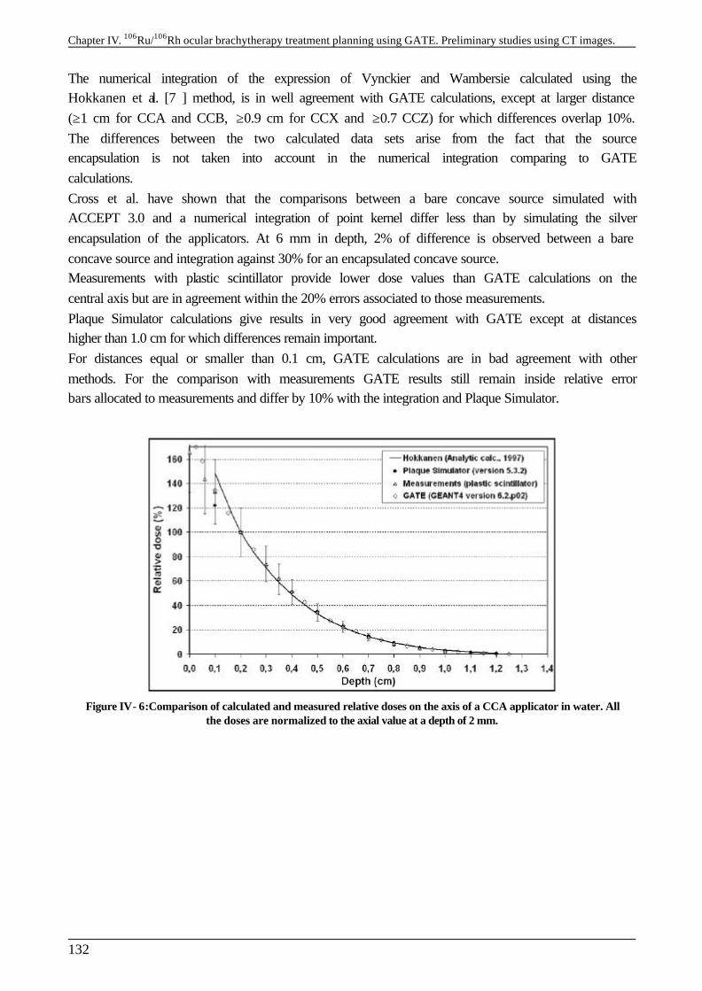
Chapter IV. 106Ru/106Rh ocular brachytherapy treatment planning using GATE. Preliminary studies using CT images.
132
The numerical integration of the expression of Vynckier and Wambersie calculated using the Hokkanen et al. [7 ] method, is in well agreement with GATE calculations, except at larger distance (≥1 cm for CCA and CCB, ≥0.9 cm for CCX and ≥0.7 CCZ) for which differences overlap 10%. The differences between the two calculated data sets arise from the fact that the source encapsulation is not taken into account in the numerical integration comparing to GATE calculations. Cross et al. have shown that the comparisons between a bare concave source simulated with ACCEPT 3.0 and a numerical integration of point kernel differ less than by simulating the silver encapsulation of the applicators. At 6 mm in depth, 2% of difference is observed between a bare concave source and integration against 30% for an encapsulated concave source. Measurements with plastic scintillator provide lower dose values than GATE calculations on the central axis but are in agreement within the 20% errors associated to those measurements. Plaque Simulator calculations give results in very good agreement with GATE except at distances higher than 1.0 cm for which differences remain important. For distances equal or smaller than 0.1 cm, GATE calculations are in bad agreement with other methods. For the comparison with measurements GATE results still remain inside relative error bars allocated to measurements and differ by 10% with the integration and Plaque Simulator.
Figure IV- 6:Comparison of calculated and measured relative doses on the axis of a CCA applicator in water. All the doses are normalized to the axial value at a depth of 2 mm.
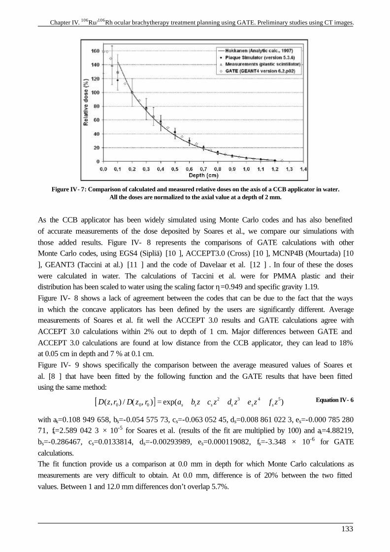
Chapter IV. 106Ru/106Rh ocular brachytherapy treatment planning using GATE. Preliminary studies using CT images.
133
Figure IV- 7: Comparison of calculated and measured relative doses on the axis of a CCB applicator in water. All the doses are normalized to the axial value at a depth of 2 mm.
As the CCB applicator has been widely simulated using Monte Carlo codes and has also benefited of accurate measurements of the dose deposited by Soares et al., we compare our simulations with those added results. Figure IV- 8 represents the comparisons of GATE calculations with other Monte Carlo codes, using EGS4 (Sipliä) [10 ], ACCEPT3.0 (Cross) [10 ], MCNP4B (Mourtada) [10 ], GEANT3 (Taccini at al.) [11 ] and the code of Davelaar et al. [12 ] . In four of these the doses were calculated in water. The calculations of Taccini et al. were for PMMA plastic and their distribution has been scaled to water using the scaling factor η=0.949 and specific gravity 1.19. Figure IV- 8 shows a lack of agreement between the codes that can be due to the fact that the ways in which the concave applicators has been defined by the users are significantly different. Average measurements of Soares et al. fit well the ACCEPT 3.0 results and GATE calculations agree with ACCEPT 3.0 calculations within 2% out to depth of 1 cm. Major differences between GATE and ACCEPT 3.0 calculations are found at low distance from the CCB applicator, they can lead to 18% at 0.05 cm in depth and 7 % at 0.1 cm. Figure IV- 9 shows specifically the comparison between the average measured values of Soares et al. [8 ] that have been fitted by the following function and the GATE results that have been fitted using the same method: [ ] 2 3 4 5
0 0 0( , ) / ( , ) exp( )s s s s s sD z r D z r a b z c z d z e z f z= + + + + + Equation IV- 6
with as=0.108 949 658, bs=-0.054 575 73, cs=-0.063 052 45, ds=0.008 861 022 3, es=-0.000 785 280 71, fs=2.589 042 3 × 10⁻⁵ for Soares et al. (results of the fit are multiplied by 100) and as=4.88219, bs=-0.286467, cs=0.0133814, ds=-0.00293989, es=0.000119082, fs=-3.348 × 10⁻⁶ for GATE calculations. The fit function provide us a comparison at 0.0 mm in depth for which Monte Carlo calculations as measurements are very difficult to obtain. At 0.0 mm, difference is of 20% between the two fitted values. Between 1 and 12.0 mm differences don’t overlap 5.7%.

Chapter IV. 106Ru/106Rh ocular brachytherapy treatment planning using GATE. Preliminary studies using CT images.
134
Figure IV- 8: Comparison of GATE calculations with other Monte Carlo codes and measurements concerning relative doses on the axis of a CCB applicator in water. All the doses are normalized to the axial value at a depth
of 1 mm.
Figure IV- 9: Comparisons of fitted GATE results with average measured values in water (Soares et al.)
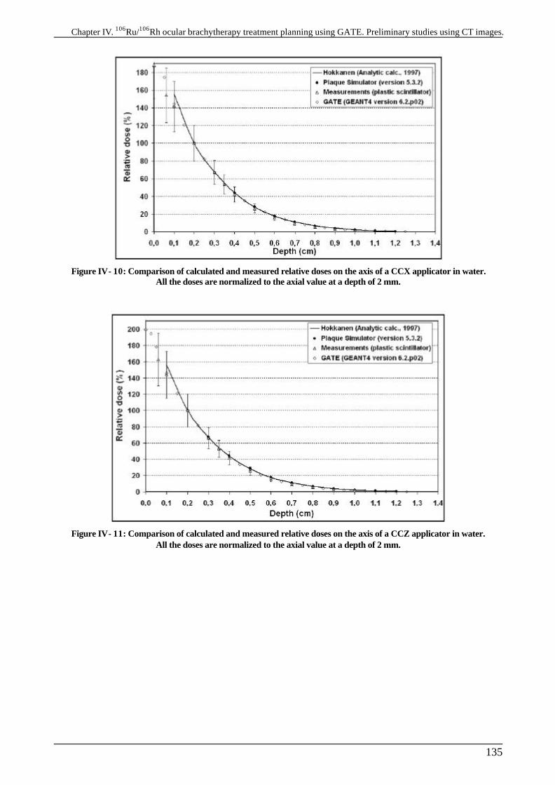
Chapter IV. 106Ru/106Rh ocular brachytherapy treatment planning using GATE. Preliminary studies using CT images.
135
Figure IV- 10: Comparison of calculated and measured relative doses on the axis of a CCX applicator in water. All the doses are normalized to the axial value at a depth of 2 mm.
Figure IV- 11: Comparison of calculated and measured relative doses on the axis of a CCZ applicator in water. All the doses are normalized to the axial value at a depth of 2 mm.
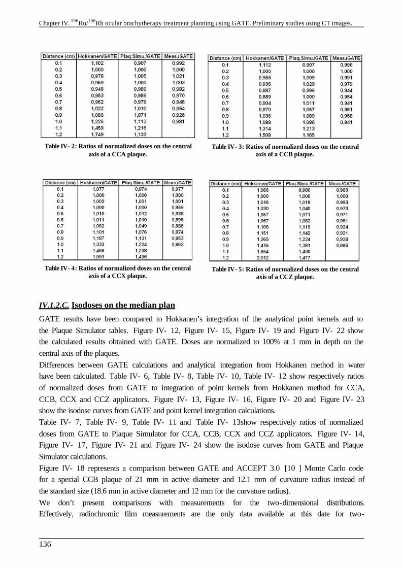
Chapter IV. 106Ru/106Rh ocular brachytherapy treatment planning using GATE. Preliminary studies using CT images.
136
Table IV- 2: Ratios of normalized doses on the central axis of a CCA plaque.
Table IV- 3: Ratios of normalized doses on the central axis of a CCB plaque.
Table IV- 4: Ratios of normalized doses on the central axis of a CCX plaque.
Table IV- 5: Ratios of normalized doses on the central axis of a CCZ plaque.
IV.1.2.C. Isodoses on the median plan
GATE results have been compared to Hokkanen’s integration of the analytical point kernels and to the Plaque Simulator tables. Figure IV- 12, Figure IV- 15, Figure IV- 19 and Figure IV- 22 show the calculated results obtained with GATE. Doses are normalized to 100% at 1 mm in depth on the central axis of the plaques. Differences between GATE calculations and analytical integration from Hokkanen method in water have been calculated. Table IV- 6, Table IV- 8, Table IV- 10, Table IV- 12 show respectively ratios of normalized doses from GATE to integration of point kernels from Hokkanen method for CCA, CCB, CCX and CCZ applicators. Figure IV- 13, Figure IV- 16, Figure IV- 20 and Figure IV- 23 show the isodose curves from GATE and point kernel integration calculations. Table IV- 7, Table IV- 9, Table IV- 11 and Table IV- 13show respectively ratios of normalized doses from GATE to Plaque Simulator for CCA, CCB, CCX and CCZ applicators. Figure IV- 14, Figure IV- 17, Figure IV- 21 and Figure IV- 24 show the isodose curves from GATE and Plaque Simulator calculations. Figure IV- 18 represents a comparison between GATE and ACCEPT 3.0 [10 ] Monte Carlo code for a special CCB plaque of 21 mm in active diameter and 12.1 mm of curvature radius instead of the standard size (18.6 mm in active diameter and 12 mm for the curvature radius). We don’t present comparisons with measurements for the two-dimensional distributions. Effectively, radiochromic film measurements are the only data available at this date for two-
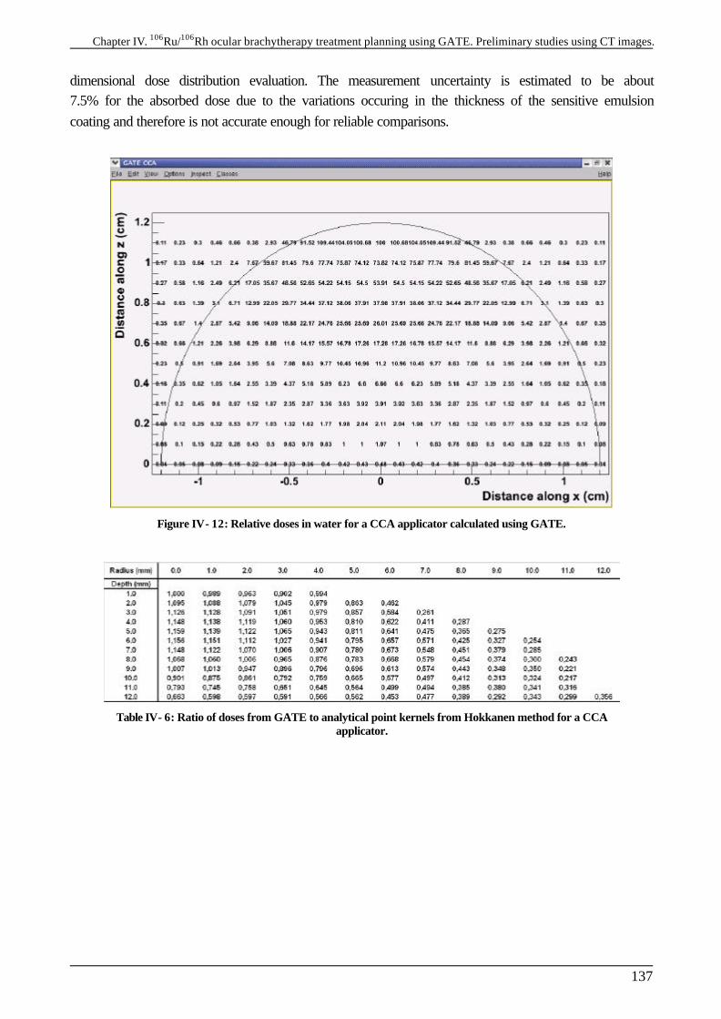
Chapter IV. 106Ru/106Rh ocular brachytherapy treatment planning using GATE. Preliminary studies using CT images.
137
dimensional dose distribution evaluation. The measurement uncertainty is estimated to be about 7.5% for the absorbed dose due to the variations occuring in the thickness of the sensitive emulsion coating and therefore is not accurate enough for reliable comparisons.
Figure IV- 12: Relative doses in water for a CCA applicator calculated using GATE.
Table IV- 6: Ratio of doses from GATE to analytical point kernels from Hokkanen method for a CCA applicator.
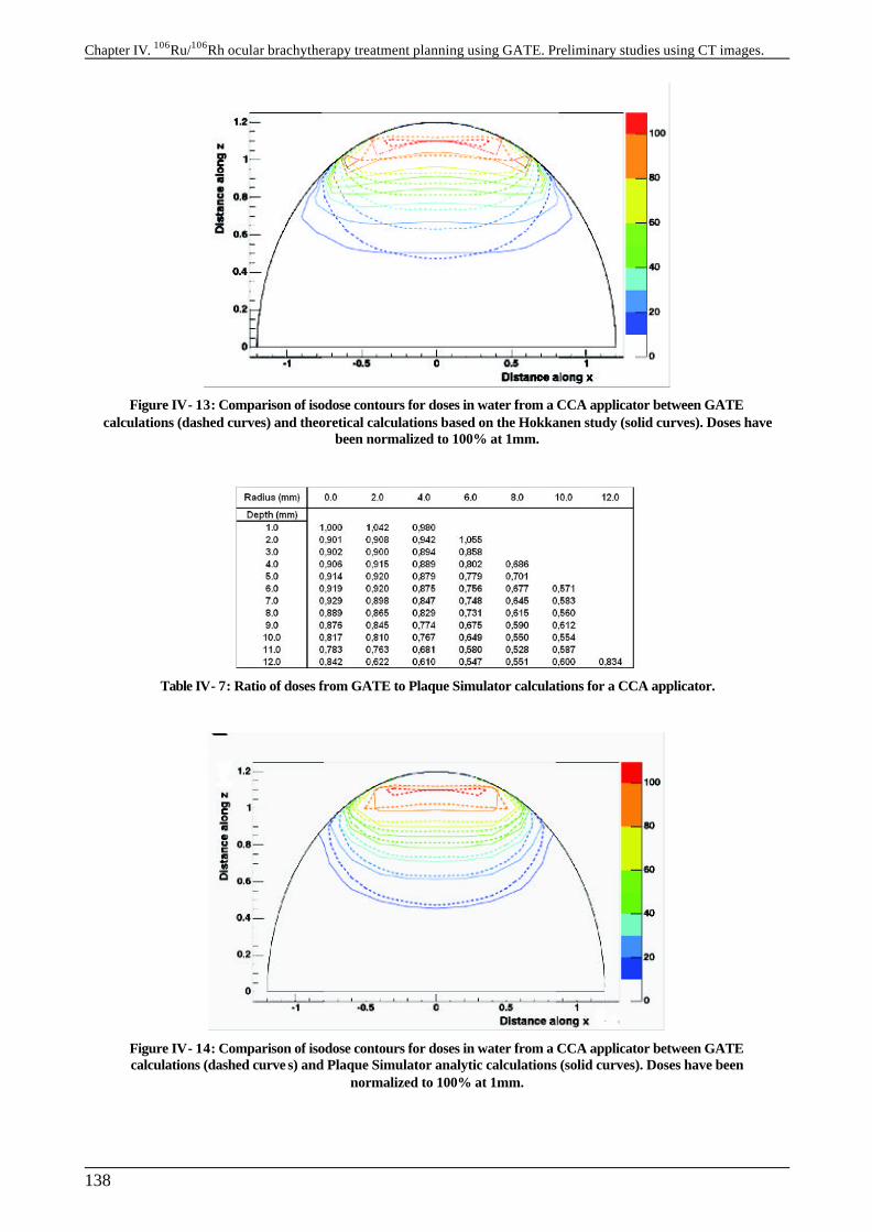
Chapter IV. 106Ru/106Rh ocular brachytherapy treatment planning using GATE. Preliminary studies using CT images.
138
Figure IV- 13: Comparison of isodose contours for doses in water from a CCA applicator between GATE calculations (dashed curves) and theoretical calculations based on the Hokkanen study (solid curves). Doses have
been normalized to 100% at 1mm.
Table IV- 7: Ratio of doses from GATE to Plaque Simulator calculations for a CCA applicator.
Figure IV- 14: Comparison of isodose contours for doses in water from a CCA applicator between GATE calculations (dashed curve s) and Plaque Simulator analytic calculations (solid curves). Doses have been
normalized to 100% at 1mm.
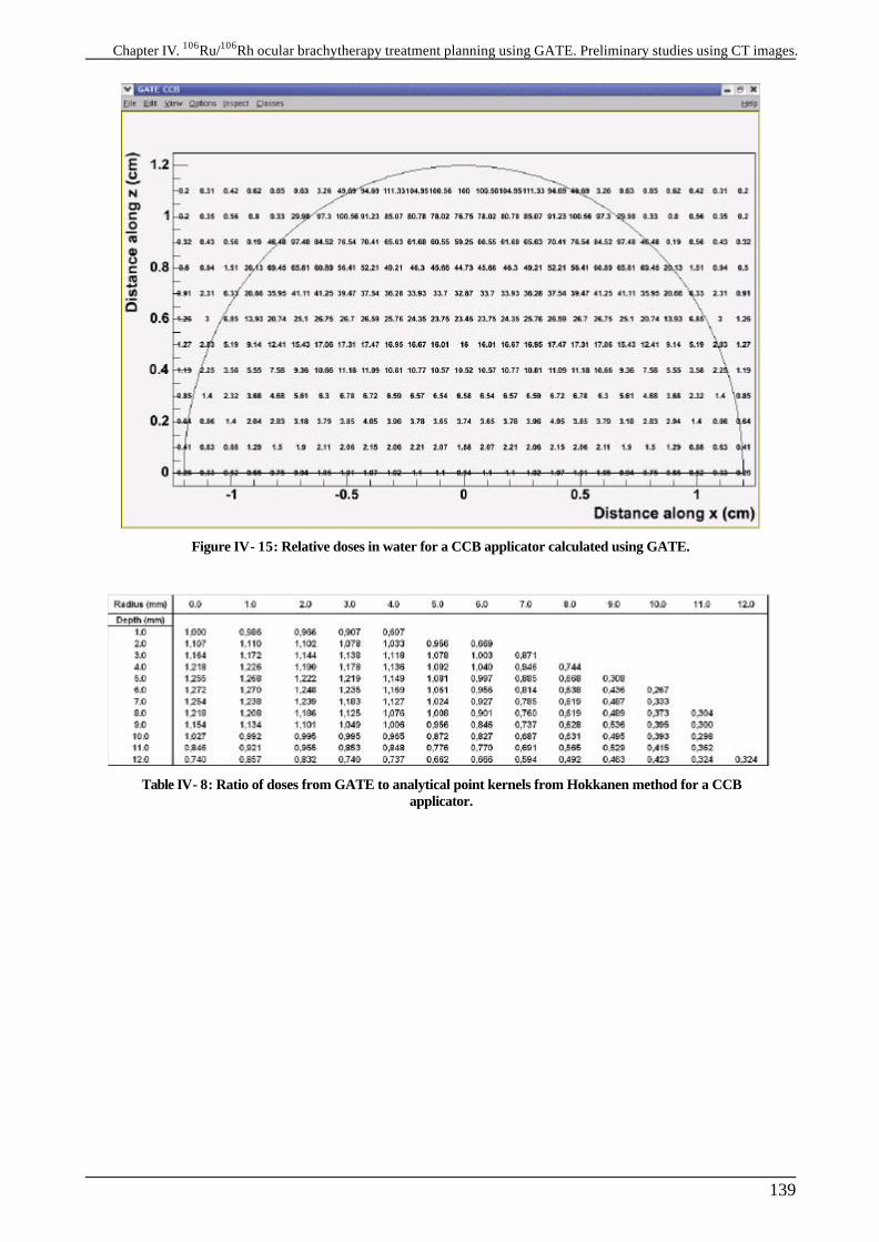
Chapter IV. 106Ru/106Rh ocular brachytherapy treatment planning using GATE. Preliminary studies using CT images.
139
Figure IV- 15: Relative doses in water for a CCB applicator calculated using GATE.
Table IV- 8: Ratio of doses from GATE to analytical point kernels from Hokkanen method for a CCB applicator.
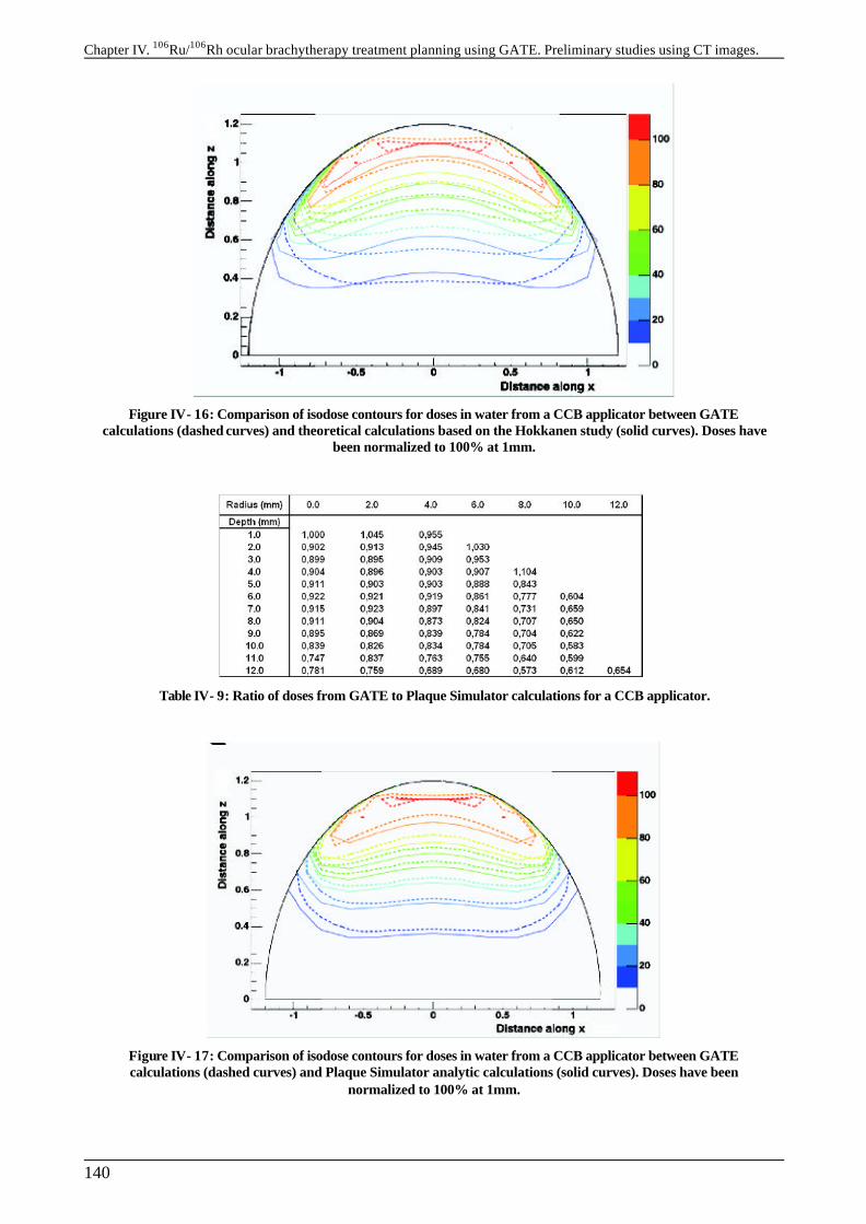
Chapter IV. 106Ru/106Rh ocular brachytherapy treatment planning using GATE. Preliminary studies using CT images.
140
Figure IV- 16: Comparison of isodose contours for doses in water from a CCB applicator between GATE calculations (dashed curves) and theoretical calculations based on the Hokkanen study (solid curves). Doses have
been normalized to 100% at 1mm.
Table IV- 9: Ratio of doses from GATE to Plaque Simulator calculations for a CCB applicator.
Figure IV- 17: Comparison of isodose contours for doses in water from a CCB applicator between GATE calculations (dashed curves) and Plaque Simulator analytic calculations (solid curves). Doses have been
normalized to 100% at 1mm.

Chapter IV. 106Ru/106Rh ocular brachytherapy treatment planning using GATE. Preliminary studies using CT images.
141
Figure IV- 18: Comparison of isodose contours for doses in water from a CCB applicator between GATE calculations (dashed curves) and ACCEPT 3.0 calculations from Cross et al. (solid curves). Doses have been
normalized to 100% at 1mm.
Figure IV- 19: Relative doses in water for a CCX applicator calculated using GATE.
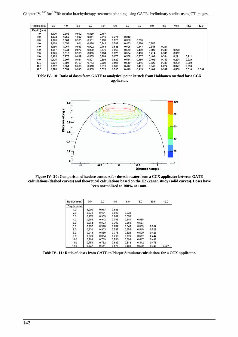
Chapter IV. 106Ru/106Rh ocular brachytherapy treatment planning using GATE. Preliminary studies using CT images.
142
Table IV- 10: Ratio of doses from GATE to analytical point kernels from Hokkanen method for a CCX applicator.
Figure IV- 20: Comparison of isodose contours for doses in water from a CCX applicator between GATE calculations (dashed curves) and theoretical calculations based on the Hokkanen study (solid curves). Doses have
been normalized to 100% at 1mm.
Table IV- 11: Ratio of doses from GATE to Plaque Simulator calculations for a CCX applicator.
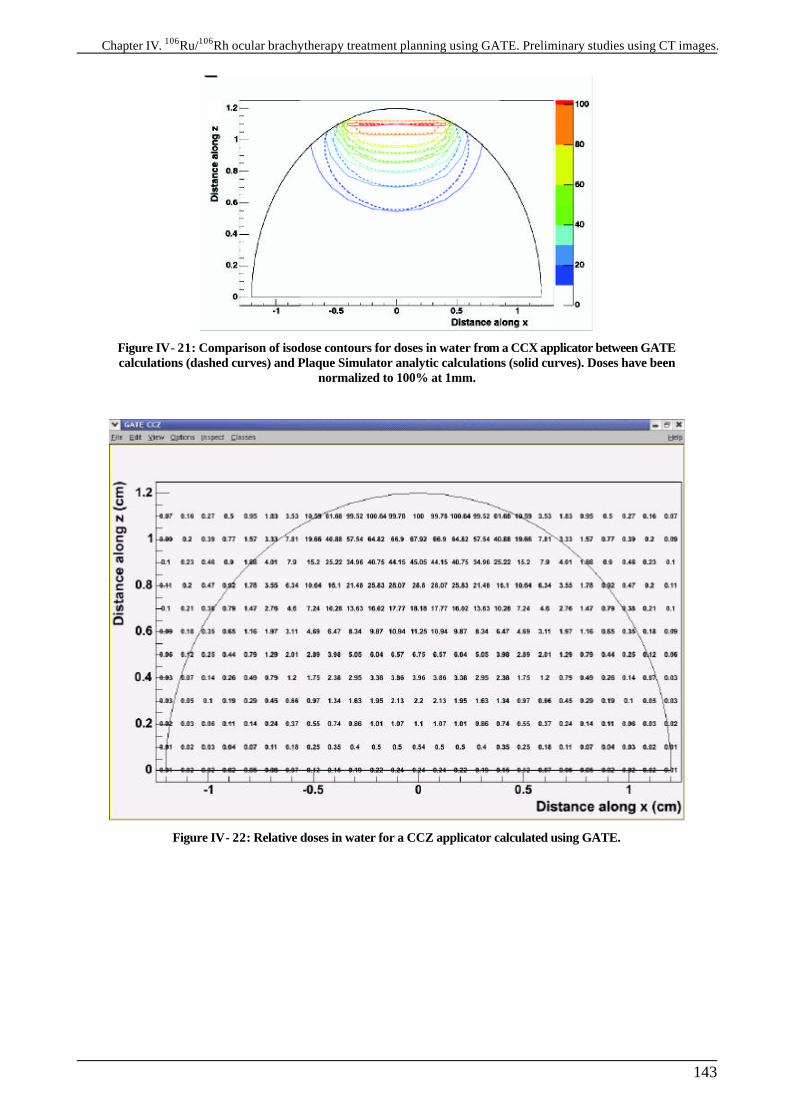
Chapter IV. 106Ru/106Rh ocular brachytherapy treatment planning using GATE. Preliminary studies using CT images.
143
Figure IV- 21: Comparison of isodose contours for doses in water from a CCX applicator between GATE calculations (dashed curves) and Plaque Simulator analytic calculations (solid curves). Doses have been
normalized to 100% at 1mm.
Figure IV- 22: Relative doses in water for a CCZ applicator calculated using GATE.
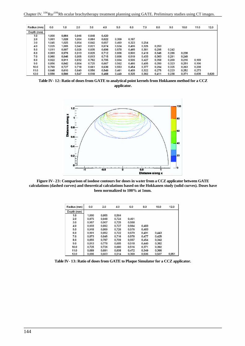
Chapter IV. 106Ru/106Rh ocular brachytherapy treatment planning using GATE. Preliminary studies using CT images.
144
Table IV- 12: Ratio of doses from GATE to analytical point kernels from Hokkanen method for a CCZ applicator.
Figure IV- 23: Comparison of isodose contours for doses in water from a CCZ applicator between GATE calculations (dashed curves) and theoretical calculations based on the Hokkanen study (solid curves). Doses have
been normalized to 100% at 1mm.
Table IV- 13: Ratio of doses from GATE to Plaque Simulator for a CCZ applicator.
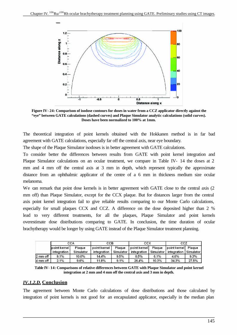
Chapter IV. 106Ru/106Rh ocular brachytherapy treatment planning using GATE. Preliminary studies using CT images.
145
Figure IV- 24: Comparison of isodose contours for doses in water from a CCZ applicator directly against the “eye” between GATE calculations (dashed curves) and Plaque Simulator analytic calculations (solid curves).
Doses have been normalized to 100% at 1mm.
The theoretical integration of point kernels obtained with the Hokkanen method is in far bad agreement with GATE calculations, especially far off the central axis, near eye boundary. The shape of the Plaque Simulator isodoses is in better agreement with GATE calculations. To consider better the differences between results from GATE with point kernel integration and Plaque Simulator calculations on an ocular treatment, we compare in Table IV- 14 the doses at 2 mm and 4 mm off the central axis at 3 mm in depth, which represent typically the approximate distance from an ophthalmic applicator of the centre of a 6 mm in thickness medium size ocular melanoma. We can remark that point dose kernels is in better agreement with GATE close to the central axis (2 mm off) than Plaque Simulator, except for the CCX plaque. But for distances larger from the central axis point kernel integration fail to give reliable results comparing to our Monte Carlo calculations, especially for small plaques CCX and CCZ. A difference on the dose deposited higher than 2 % lead to very different treatments, for all the plaques, Plaque Simulator and point kernels overestimate dose distributions comparing to GATE. In conclusion, the time duration of ocular brachytherapy would be longer by using GATE instead of the Plaque Simulator treatment planning.
Table IV- 14: Comparisons of relative differences between GATE with Plaque Simulator and point kernel integration at 2 mm and 4 mm off the central axis and 3 mm in depth.
IV.1.2.D. Conclusion
The agreement between Monte Carlo calculations of dose distributions and those calculated by integration of point kernels is not good for an encapsulated applicator, especially in the median plan
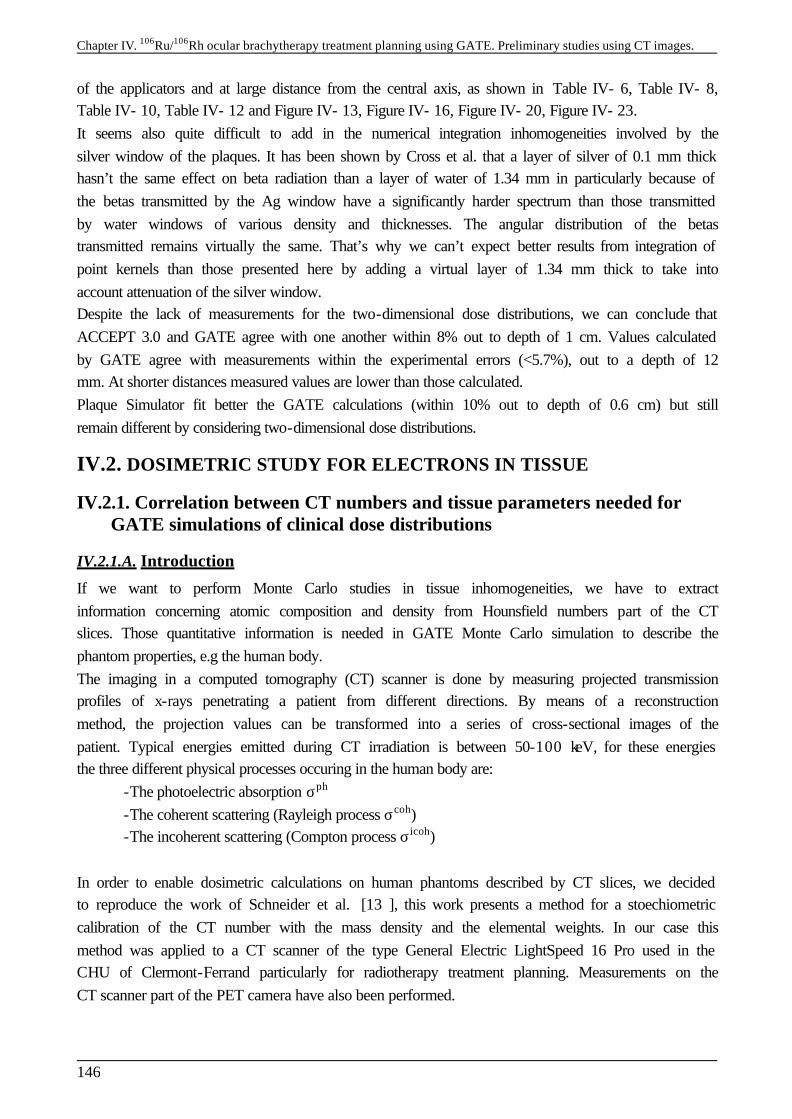
Chapter IV. 106Ru/106Rh ocular brachytherapy treatment planning using GATE. Preliminary studies using CT images.
146
of the applicators and at large distance from the central axis, as shown in Table IV- 6, Table IV- 8, Table IV- 10, Table IV- 12 and Figure IV- 13, Figure IV- 16, Figure IV- 20, Figure IV- 23. It seems also quite difficult to add in the numerical integration inhomogeneities involved by the silver window of the plaques. It has been shown by Cross et al. that a layer of silver of 0.1 mm thick hasn’t the same effect on beta radiation than a layer of water of 1.34 mm in particularly because of the betas transmitted by the Ag window have a significantly harder spectrum than those transmitted by water windows of various density and thicknesses. The angular distribution of the betas transmitted remains virtually the same. That’s why we can’t expect better results from integration of point kernels than those presented here by adding a virtual layer of 1.34 mm thick to take into account attenuation of the silver window. Despite the lack of measurements for the two-dimensional dose distributions, we can conclude that ACCEPT 3.0 and GATE agree with one another within 8% out to depth of 1 cm. Values calculated by GATE agree with measurements within the experimental errors (<5.7%), out to a depth of 12 mm. At shorter distances measured values are lower than those calculated. Plaque Simulator fit better the GATE calculations (within 10% out to depth of 0.6 cm) but still remain different by considering two-dimensional dose distributions.
IV.2. DOSIMETRIC STUDY FOR ELECTRONS IN TISSUE
IV.2.1. Correlation between CT numbers and tissue parameters needed for GATE simulations of clinical dose distributions
IV.2.1.A. Introduction
If we want to perform Monte Carlo studies in tissue inhomogeneities, we have to extract information concerning atomic composition and density from Hounsfield numbers part of the CT slices. Those quantitative information is needed in GATE Monte Carlo simulation to describe the phantom properties, e.g the human body. The imaging in a computed tomography (CT) scanner is done by measuring projected transmission profiles of x-rays penetrating a patient from different directions. By means of a reconstruction method, the projection values can be transformed into a series of cross-sectional images of the patient. Typical energies emitted during CT irradiation is between 50-100 keV, for these energies the three different physical processes occuring in the human body are:
-The photoelectric absorption σph
-The coherent scattering (Rayleigh process σcoh) -The incoherent scattering (Compton process σicoh) In order to enable dosimetric calculations on human phantoms described by CT slices, we decided to reproduce the work of Schneider et al. [13 ], this work presents a method for a stoechiometric calibration of the CT number with the mass density and the elemental weights. In our case this method was applied to a CT scanner of the type General Electric LightSpeed 16 Pro used in the CHU of Clermont-Ferrand particularly for radiotherapy treatment planning. Measurements on the CT scanner part of the PET camera have also been performed.

Chapter IV. 106Ru/106Rh ocular brachytherapy treatment planning using GATE. Preliminary studies using CT images.
147
IV.2.1.B. X-ray attenuation coefficient and CT numbers
The linear attenuation coefficient µ(E,t) of a tissue at position t along the projection line with length s is defined by the following equation:
1
( ) ( )n
iA i
i i
E N EAω
µ ρ σ=
=
∑ Equation IV-5
with ρ (g.cm-3) the mass density, NA(mol-1) the Avogadro constant (6.022045 × 10²³), I the element index, ωi the elemental weight, σi (barn/atom) the total cross section σi
ph+σicoh+σi
icoh and Ai (g mol-1) the atomic mass. In all this study, we will assume that the reconstructed attenuation values of the different tissues are completely independent of the location of the tissues. The mean attenuation can then be described in function of the polychromatic spectrum of x-rays defined by the independent spectral function
( )f E∧
as:
__ ( ) ( , )
( )( )
f E E s dEs
f E dE
µµ
∧
∧= ∫∫
Equation IV-6
The values of __
µ are then converted into Hounsfield units H (CT numbers):
__
__
2
1 1000H O
Hµ
µ
= −
Equation IV-7
This CT number is defined in such way that water has always the value 0 and air the value –1000. As it is noticed by Schneider, the ratio (
__ __
2/ H Oµ µ ) slightly depends on the spectral function f∧
(E) and therefore the CT number is scanner-dependent quantity with fixed values for water and air. We can then rely the tissue parameters (density and elemental weights) with the Hounsfield units, e.g the ratio (
__ __
2/ H Oµ µ ) with the equation:
____
__12
2
1 1( )
ni
iAiH O i
H O
N EAωµ
σρ µµ =
=
∑
Equation IV-8
IV.2.1.C. Calculation of the CT numbers of human tissues
For the range of diagnostic x-ray energies and the elements contained in human tissues, the total cross section can be expressed by the following approximation shown by Rutherford et al. (1976) [14 ]:
2.86 4.62( ) ( ) ( ) ( )KN sca phi i i iE Z K E Z K E Z K Eσ = + + Equation IV-9
with KKN denoting the Klein-Nishina coefficient, Ksca defining the coherent scattering as well as the binding correction for the incoherent scattering and Kph the photoelectric absorption.
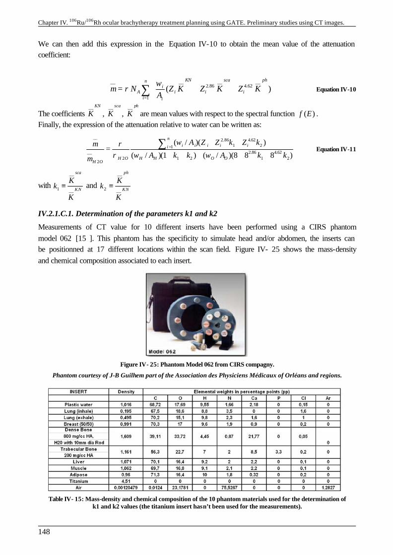
Chapter IV. 106Ru/106Rh ocular brachytherapy treatment planning using GATE. Preliminary studies using CT images.
148
We can then add this expression in the Equation IV-10 to obtain the mean value of the attenuation coefficient:
__ __ __ __
2.86 4.62
1
( )KN sca phn
iA i i i
i i
N Z K Z K Z KAω
µ ρ=
= + +
∑ Equation IV-10
The coefficients __ KN
K , __ sca
K , __ ph
K are mean values with respect to the spectral function ( )f E∧
. Finally, the expression of the attenuation relative to water can be written as:
__ 2.86 4.621 21
__ 2.86 4.622 1 2 1 2
2
( / )( )
( / )(1 ) ( / )(8 8 8 )
ni i i i ii
H O H H O OH O
A Z Z k Z k
A k k A k k
ωµ ρρ ω ωµ
=+ +
=+ + + + +
∑ Equation IV-11
with
__
1 __
sca
KN
Kk
K≡ and
__
2 __
ph
KN
Kk
K≡
IV.2.1.C.1. Determination of the parameters k1 and k2
Measurements of CT value for 10 different inserts have been performed using a CIRS phantom model 062 [15 ]. This phantom has the specificity to simulate head and/or abdomen, the inserts can be positionned at 17 different locations within the scan field. Figure IV- 25 shows the mass-density and chemical composition associated to each insert.
Figure IV- 25: Phantom Model 062 from CIRS compagny.
Phantom courtesy of J-B Guilhem part of the Association des Physiciens Médicaux of Orléans and regions.
Table IV- 15: Mass-density and chemical composition of the 10 phantom materials used for the determination of k1 and k2 values (the titanium insert hasn’t been used for the measurements).
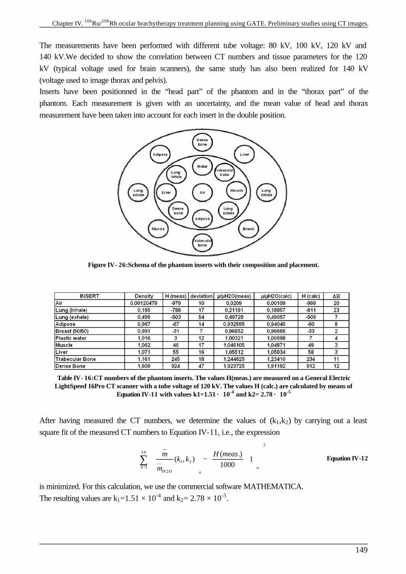
Chapter IV. 106Ru/106Rh ocular brachytherapy treatment planning using GATE. Preliminary studies using CT images.
149
The measurements have been performed with different tube voltage: 80 kV, 100 kV, 120 kV and 140 kV.We decided to show the correlation between CT numbers and tissue parameters for the 120 kV (typical voltage used for brain scanners), the same study has also been realized for 140 kV (voltage used to image thorax and pelvis). Inserts have been positionned in the “head part” of the phantom and in the “thorax part” of the phantom. Each measurement is given with an uncertainty, and the mean value of head and thorax measurement have been taken into account for each insert in the double position.
Figure IV- 26:Schema of the phantom inserts with their composition and placement.
Table IV- 16:CT numbers of the phantom inserts. The values H(meas.) are measured on a General Electric LightSpeed 16Pro CT scanner with a tube voltage of 120 kV. The values H (calc.) are calculated by means of
Equation IV-11 with values k1=1.51 × 10⁻⁴ and k2= 2.78 × 10⁻⁵
After having measured the CT numbers, we determine the values of (k1,k2) by carrying out a least square fit of the measured CT numbers to Equation IV-11, i.e., the expression
2__
10
1 2__1
2
( .)( , ) 1
1000n nH O n
H meask k
µ
µ=
− + ∑ Equation IV-12
is minimized. For this calculation, we use the commercial software MATHEMATICA. The resulting values are k1=1.51 × 10⁻⁴ and k2= 2.78 × 10⁻⁵.

Chapter IV. 106Ru/106Rh ocular brachytherapy treatment planning using GATE. Preliminary studies using CT images.
150
Figure IV- 27:Calculated versus measured Hounsfield units of the phantom inserts (values listed in Table IV- 16).
Then, by means of Equation IV-7 and Equation IV-11 together with the above values of k1 and k2 we have calculated the CT numbers of 71 human tissues, whose mass densities and elemental weights are taken from the literature [16 ][17 ]. They are listed in Table IV- 17 and Table IV- 18 respectively for soft and skeletal tissues.
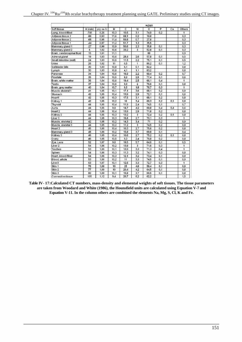
Chapter IV. 106Ru/106Rh ocular brachytherapy treatment planning using GATE. Preliminary studies using CT images.
151
Table IV- 17:Calculated CT numbers, mass-density and elemental weights of soft tissues. The tissue parameters are taken from Woodard and White (1986), the Hounsfield units are calculated using Equation V-7 and
Equation V-11. In the column others are combined the elements Na, Mg, S, Cl, K and Fe.
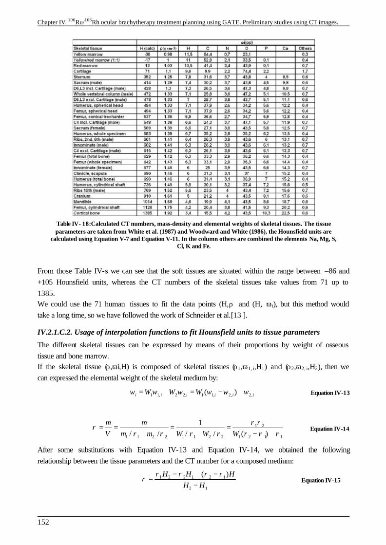
Chapter IV. 106Ru/106Rh ocular brachytherapy treatment planning using GATE. Preliminary studies using CT images.
152
Table IV- 18:Calculated CT numbers, mass-density and elemental weights of skeletal tissues. The tissue parameters are taken from White et al. (1987) and Woodward and White (1986), the Hounsfield units are
calculated using Equation V-7 and Equation V-11. In the column others are combined the elements Na, Mg, S, Cl, K and Fe.
From those Table IV-s we can see that the soft tissues are situated within the range between –86 and +105 Hounsfield units, whereas the CT numbers of the skeletal tissues take values from 71 up to 1385. We could use the 71 human tissues to fit the data points (H,ρ) and (H, ωi), but this method would take a long time, so we have followed the work of Schneider et al.[13 ].
IV.2.1.C.2. Usage of interpolation functions to fit Hounsfield units to tissue parameters
The different skeletal tissues can be expressed by means of their proportions by weight of osseous tissue and bone marrow. If the skeletal tissue (ρ,ωi,H) is composed of skeletal tissues (ρ1,ω1, i,H1) and (ρ2,ω2, i,H2), then we can expressed the elemental weight of the skeletal medium by:
1 1, 2 2, 1 1, 2, 2,( )i i i i i iW W Wω ω ω ω ω ω= + = − + Equation IV-13
1 2
1 1 2 2 1 1 2 2 1 2 1 1
1/ / / / ( )
m mV m m W W W
ρ ρρ
ρ ρ ρ ρ ρ ρ ρ= = = =
+ + − + Equation IV-14
After some substitutions with Equation IV-13 and Equation IV-14, we obtained the following relationship between the tissue parameters and the CT number for a composed medium:
1 2 2 1 2 1
2 1
( )H H HH H
ρ ρ ρ ρρ
− + −=
− Equation IV-15
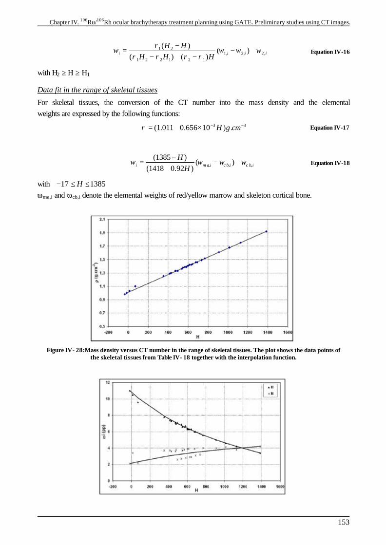
Chapter IV. 106Ru/106Rh ocular brachytherapy treatment planning using GATE. Preliminary studies using CT images.
153
1 2
1, 2, 2,1 2 2 1 2 1
( )( )
( ) ( )i i i i
H HH H H
ρω ω ω ω
ρ ρ ρ ρ−
= − +− + −
Equation IV-16
with H2 ≥ H ≥ H1
Data fit in the range of skeletal tissues
For skeletal tissues, the conversion of the CT number into the mass density and the elemental weights are expressed by the following functions:
3 3(1.011 0.656 10 ) .H g cmρ − −= + × Equation IV-17
, , ,(1385 )
( )(1418 0.92 )i m a i c b i c b i
HH
ω ω ω ω−
= − ++
Equation IV-18
with 17 1385H− ≤ ≤ ωma,i and ωcb,i denote the elemental weights of red/yellow marrow and skeleton cortical bone.
Figure IV- 28:Mass density versus CT number in the range of skeletal tissues. The plot shows the data points of the skeletal tissues from Table IV- 18 together with the interpolation function.
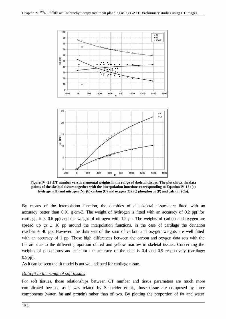
Chapter IV. 106Ru/106Rh ocular brachytherapy treatment planning using GATE. Preliminary studies using CT images.
154
Figure IV- 29:CT number versus elemental weights in the range of skeletal tissues. The plot shows the data points of the skeletal tissues together with the interpolation functions corresponding to Equation IV-18: (a)
hydrogen (H) and nitrogen (N), (b) carbon (C) and oxygen (O), (c) phosphorus (P) and calcium (Ca).
By means of the interpolation function, the densities of all skeletal tissues are fitted with an accuracy better than 0.01 g.cm-3. The weight of hydrogen is fitted with an accuracy of 0.2 pp( for cartilage, it is 0.6 pp) and the weight of nitrogen with 1.2 pp. The weights of carbon and oxygen are spread up to ± 10 pp around the interpolation functions, in the case of cartilage the deviation reaches ± 40 pp. However, the data sets of the sum of carbon and oxygen weights are well fitted with an accuracy of 1 pp. Those high differences between the carbon and oxygen data sets with the fits are due to the different proportion of red and yellow marrow in skeletal tissues. Concerning the weights of phosphorus and calcium the accuracy of the data is 0.4 and 0.9 respectively (cartilage: 0.9pp). As it can be seen the fit model is not well adapted for cartilage tissue.
Data fit in the range of soft tissues
For soft tissues, those relationships between CT number and tissue parameters are much more complicated because as it was related by Schneider et al., those tissue are composed by three components (water, fat and protein) rather than of two. By plotting the proportion of fat and water

Chapter IV. 106Ru/106Rh ocular brachytherapy treatment planning using GATE. Preliminary studies using CT images.
155
of the soft tissues between Adipose tissue3 and Connective tissue, we can remarked that those tissues are divided in two parts following their composition: adrenal tissue 3 to adrenal gland and Small intestine to connective tissue. The interpolation functions obtained for the fit of soft tissues are: For the tissues between adipose tissue 3 (at) and adrenal gland (ag):
3 3(1.012 0.952 10 ) .H g cmρ − −= + × Equation IV-19
, , ,(17.67 0.93 )
( )(106.25 0.1 )i a t i ag i a g i
HH
ω ω ω ω−
= − ++
Equation IV-20
with 86 19H− ≤ ≤ For the tissues between small intestine (si) and connective tissue (ct):
3 3(1.003 1.110 10 ) .H g cmρ − −= + × Equation IV-21
, , ,(108.15 1.03 )
( )(81.27 0.09 )i si i c t i c t i
HH
ω ω ω ω−
= − ++
Equation IV-22
with 24 105H≤ ≤ Plots of the functions together with the data points for soft tissues are shown in Figure IV- 30 and Figure IV- 31. The data points of the mass density are fitted with an accuracy better than 0.02 g.cm-3. The weights of hydrogen and nitrogen are respectively fitted with an accuracy better than 0.1 and 2.5 respectively for the range of soft tissues between adipose tissue3 and adrenal gland, and are better than 0.4 and 2.4 in the range between small intestine and connective tissue. The weights of carbon and oxygen are respectively not well fitted (accuracy of 30.0 and 32.0 pp for at-ag, 11.2 and 11.4 pp for si-ct). The sum of carbon and oxygen weights are fitted with an accuracy of 2pp.
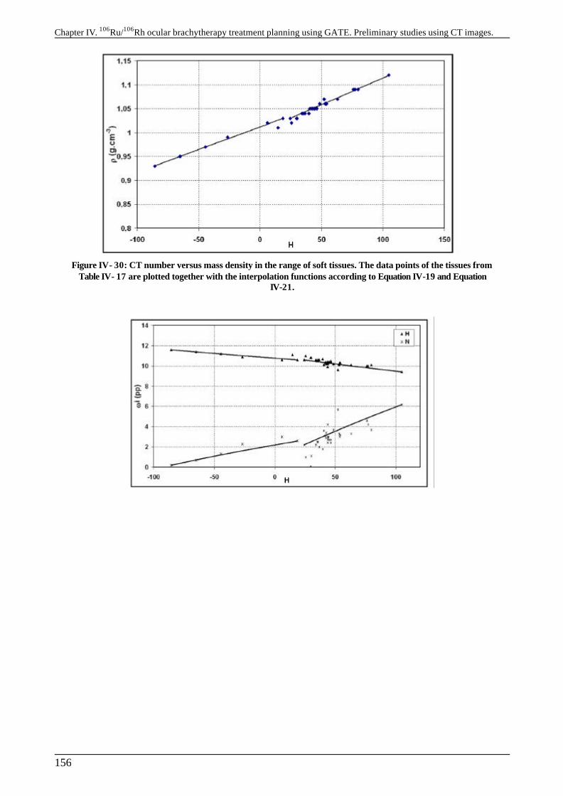
Chapter IV. 106Ru/106Rh ocular brachytherapy treatment planning using GATE. Preliminary studies using CT images.
156
Figure IV- 30: CT number versus mass density in the range of soft tissues. The data points of the tissues from Table IV- 17 are plotted together with the interpolation functions according to Equation IV-19 and Equation
IV-21.
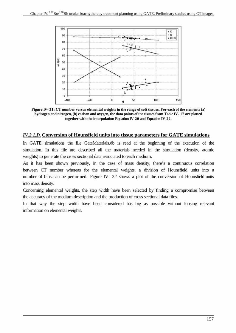
Chapter IV. 106Ru/106Rh ocular brachytherapy treatment planning using GATE. Preliminary studies using CT images.
157
Figure IV- 31: CT number versus elemental weights in the range of soft tissues. For each of the elements (a) hydrogen and nitrogen, (b) carbon and oxygen, the data points of the tissues from Table IV- 17 are plotted
together with the interpolation Equation IV-20 and Equation IV-22.
IV.2.1.D. Conversion of Hounsfield units into tissue parameters for GATE simulations
In GATE simulations the file GateMaterials.db is read at the beginning of the execution of the simulation. In this file are described all the materials needed in the simulation (density, atomic weights) to generate the cross sectional data associated to each medium. As it has been shown previously, in the case of mass density, there’s a continuous correlation between CT number whereas for the elemental weights, a division of Hounsfield units into a number of bins can be performed. Figure IV- 32 shows a plot of the conversion of Hounsfield units into mass density. Concerning elemental weights, the step width have been selected by finding a compromise between the accuracy of the medium description and the production of cross sectional data files. In that way the step width have been considered has big as possible without loosing relevant information on elemental weights.
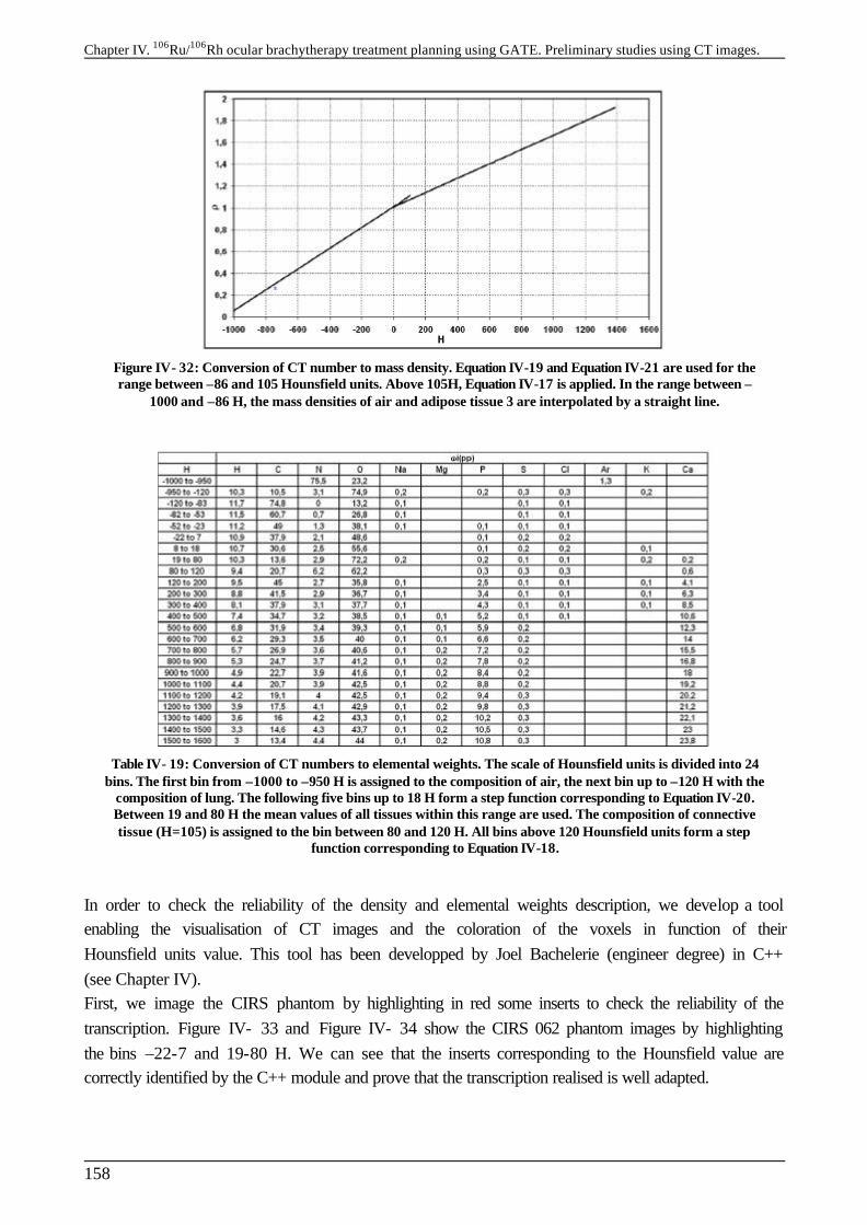
Chapter IV. 106Ru/106Rh ocular brachytherapy treatment planning using GATE. Preliminary studies using CT images.
158
Figure IV- 32: Conversion of CT number to mass density. Equation IV-19 and Equation IV-21 are used for the range between –86 and 105 Hounsfield units. Above 105H, Equation IV-17 is applied. In the range between –
1000 and –86 H, the mass densities of air and adipose tissue 3 are interpolated by a straight line.
Table IV- 19: Conversion of CT numbers to elemental weights. The scale of Hounsfield units is divided into 24 bins. The first bin from –1000 to –950 H is assigned to the composition of air, the next bin up to –120 H with the
composition of lung. The following five bins up to 18 H form a step function corresponding to Equation IV-20. Between 19 and 80 H the mean values of all tissues within this range are used. The composition of connective tissue (H=105) is assigned to the bin between 80 and 120 H. All bins above 120 Hounsfield units form a step
function corresponding to Equation IV-18.
In order to check the reliability of the density and elemental weights description, we develop a tool enabling the visualisation of CT images and the coloration of the voxels in function of their Hounsfield units value. This tool has been developped by Joel Bachelerie (engineer degree) in C++ (see Chapter IV). First, we image the CIRS phantom by highlighting in red some inserts to check the reliability of the transcription. Figure IV- 33 and Figure IV- 34 show the CIRS 062 phantom images by highlighting the bins –22-7 and 19-80 H. We can see that the inserts corresponding to the Hounsfield value are correctly identified by the C++ module and prove that the transcription realised is well adapted.
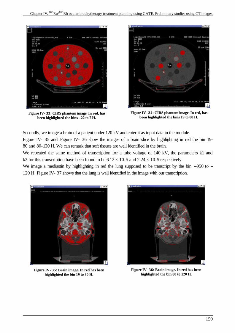
Chapter IV. 106Ru/106Rh ocular brachytherapy treatment planning using GATE. Preliminary studies using CT images.
159
Figure IV- 33: CIRS phantom image. In red, has been highlighted the bins –22 to 7 H.
Figure IV- 34: CIRS phantom image. In red, has been highlighted the bins 19 to 80 H.
Secondly, we image a brain of a patient under 120 kV and enter it as input data in the module. Figure IV- 35 and Figure IV- 36 show the images of a brain slice by highlighting in red the bin 19-80 and 80-120 H. We can remark that soft tissues are well identified in the brain. We repeated the same method of transcription for a tube voltage of 140 kV, the parameters k1 and k2 for this transcription have been found to be 6.12 × 10⁻⁵ and 2.24 × 10⁻⁵ respectively. We image a mediastin by highlighting in red the lung supposed to be transcript by the bin –950 to –120 H. Figure IV- 37 shows that the lung is well identified in the image with our transcription.
Figure IV- 35: Brain image. In red has been highlighted the bin 19 to 80 H.
Figure IV- 36: Brain image. In red has been highlighted the bin 80 to 120 H.
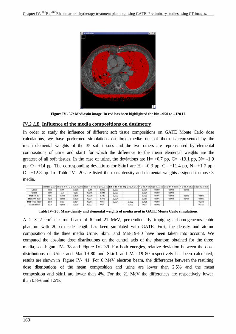
Chapter IV. 106Ru/106Rh ocular brachytherapy treatment planning using GATE. Preliminary studies using CT images.
160
Figure IV- 37: Mediastin image. In red has been highlighted the bin –950 to –120 H.
IV.2.1.E. Influence of the media compositions on dosimetry
In order to study the influence of different soft tissue compositions on GATE Monte Carlo dose calculations, we have performed simulations on three media: one of them is represented by the mean elemental weights of the 35 soft tissues and the two others are reprensented by elemental compositions of urine and skin1 for which the difference to the mean elemental weights are the greatest of all soft tissues. In the case of urine, the deviations are H= +0.7 pp, C= -13.1 pp, N= -1.9 pp, O= +14 pp. The corresponding deviations for Skin1 are H= -0.3 pp, C= +11.4 pp, N= +1.7 pp, O= +12.8 pp. In Table IV- 20 are listed the mass-density and elemental weights assigned to those 3 media.
Table IV- 20: Mass-density and elemental weights of media used in GATE Monte Carlo simulations.
A 2 × 2 cm2 electron beam of 6 and 21 MeV, perpendicularly impiging a homogeneous cubic phantom with 20 cm side length has been simulated with GATE. First, the density and atomic composition of the three media Urine, Skin1 and Mat-19-80 have been taken into account. We compared the absolute dose distributions on the central axis of the phantom obtained for the three media, see Figure IV- 38 and Figure IV- 39. For both energies, relative deviation between the dose distributions of Urine and Mat-19-80 and Skin1 and Mat-19-80 respectively has been calculated, results are shown in Figure IV- 41. For 6 MeV electron beam, the differences between the resulting dose distributions of the mean composition and urine are lower than 2.5% and the mean composition and skin1 are lower than 4%. For the 21 MeV the differences are respectively lower than 0.8% and 1.5%.
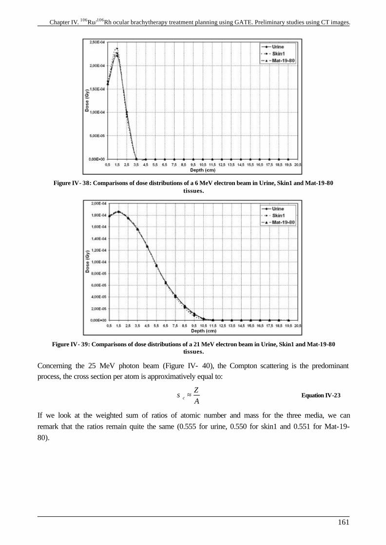
Chapter IV. 106Ru/106Rh ocular brachytherapy treatment planning using GATE. Preliminary studies using CT images.
161
Figure IV- 38: Comparisons of dose distributions of a 6 MeV electron beam in Urine, Skin1 and Mat-19-80 tissues.
Figure IV- 39: Comparisons of dose distributions of a 21 MeV electron beam in Urine, Skin1 and Mat-19-80 tissues.
Concerning the 25 MeV photon beam (Figure IV- 40), the Compton scattering is the predominant process, the cross section per atom is approximatively equal to:
c
ZA
σ ≈ Equation IV-23
If we look at the weighted sum of ratios of atomic number and mass for the three media, we can remark that the ratios remain quite the same (0.555 for urine, 0.550 for skin1 and 0.551 for Mat-19-80).
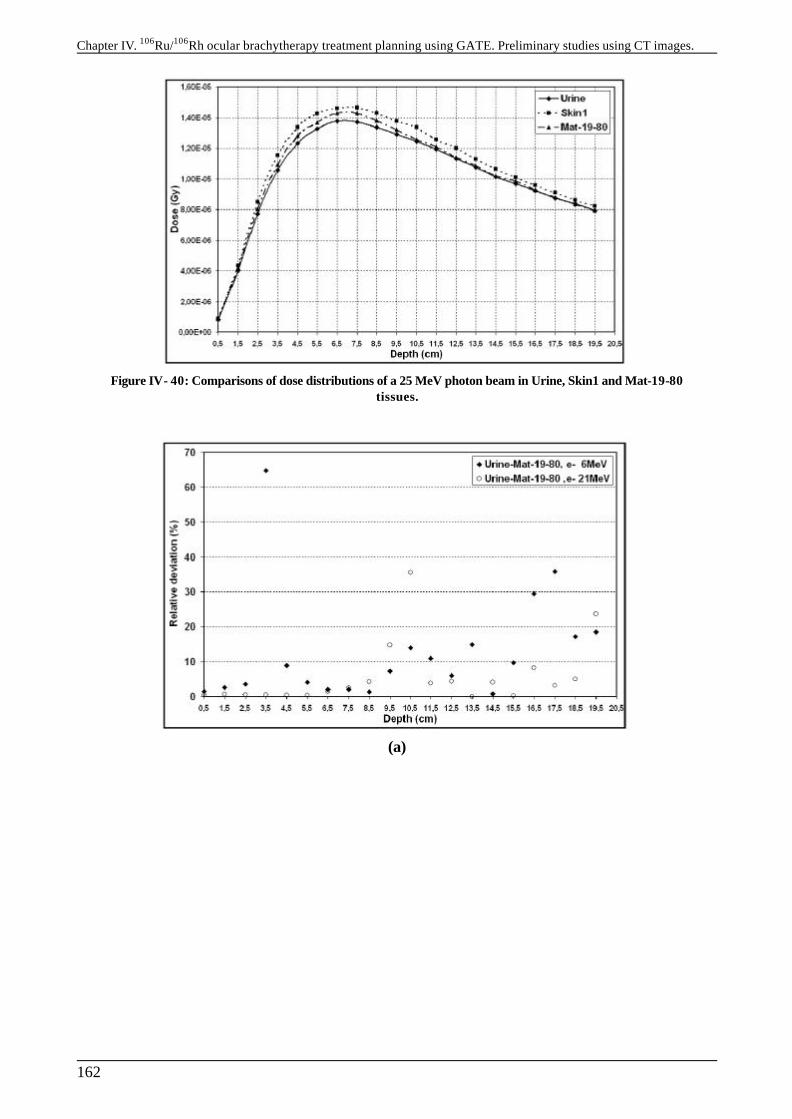
Chapter IV. 106Ru/106Rh ocular brachytherapy treatment planning using GATE. Preliminary studies using CT images.
162
Figure IV- 40: Comparisons of dose distributions of a 25 MeV photon beam in Urine, Skin1 and Mat-19-80 tissues.
(a)
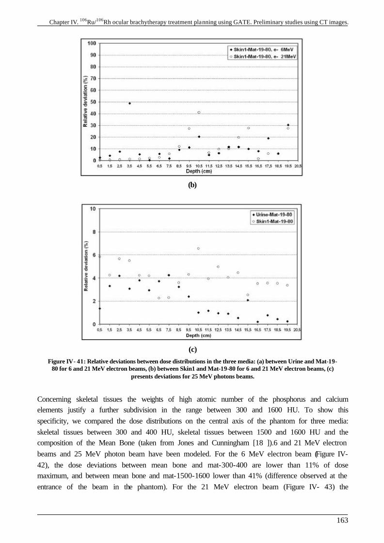
Chapter IV. 106Ru/106Rh ocular brachytherapy treatment planning using GATE. Preliminary studies using CT images.
163
(b)
(c) Figure IV- 41: Relative deviations between dose distributions in the three media: (a) between Urine and Mat-19-
80 for 6 and 21 MeV electron beams, (b) between Skin1 and Mat-19-80 for 6 and 21 MeV electron beams, (c) presents deviations for 25 MeV photons beams.
Concerning skeletal tissues the weights of high atomic number of the phosphorus and calcium elements justify a further subdivision in the range between 300 and 1600 HU. To show this specificity, we compared the dose distributions on the central axis of the phantom for three media: skeletal tissues between 300 and 400 HU, skeletal tissues between 1500 and 1600 HU and the composition of the Mean Bone (taken from Jones and Cunningham [18 ]).6 and 21 MeV electron beams and 25 MeV photon beam have been modeled. For the 6 MeV electron beam (Figure IV- 42), the dose deviations between mean bone and mat-300-400 are lower than 11% of dose maximum, and between mean bone and mat-1500-1600 lower than 41% (difference observed at the entrance of the beam in the phantom). For the 21 MeV electron beam (Figure IV- 43) the
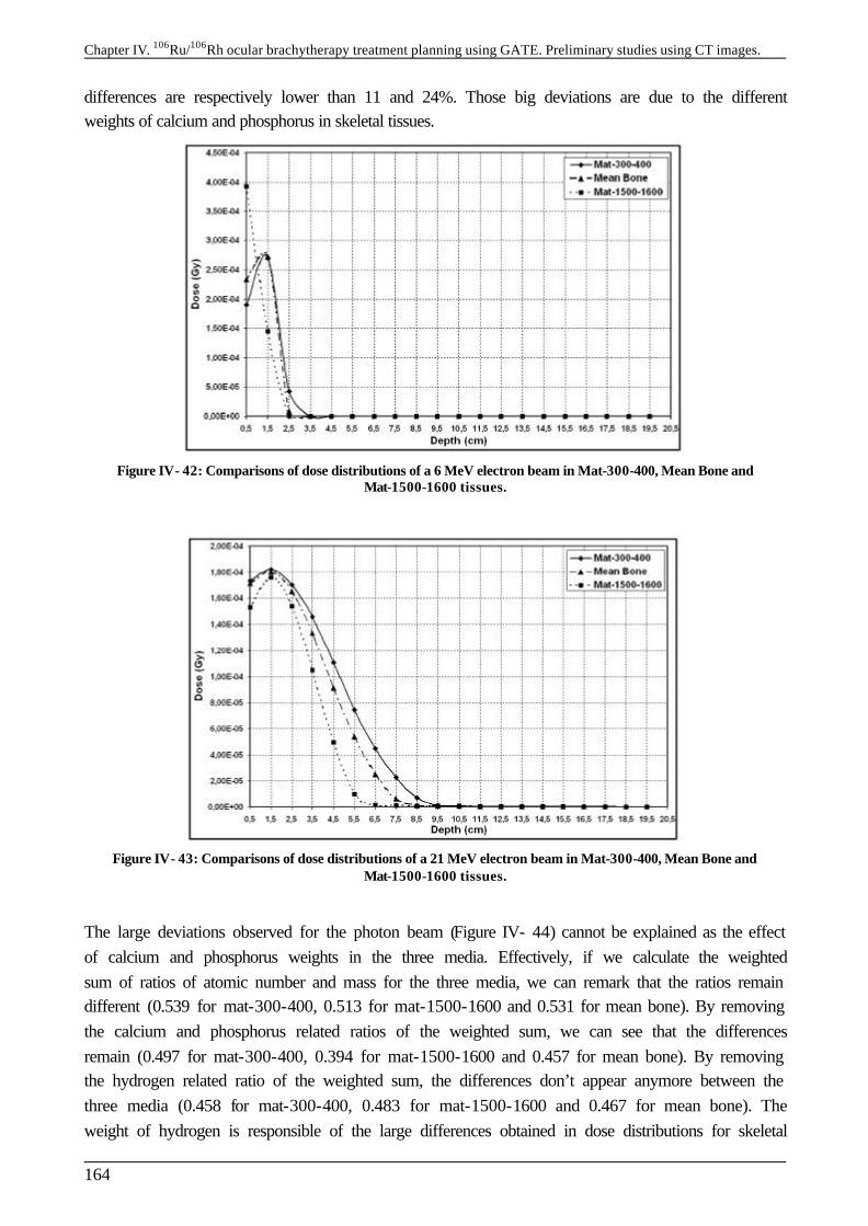
Chapter IV. 106Ru/106Rh ocular brachytherapy treatment planning using GATE. Preliminary studies using CT images.
164
differences are respectively lower than 11 and 24%. Those big deviations are due to the different weights of calcium and phosphorus in skeletal tissues.
Figure IV- 42: Comparisons of dose distributions of a 6 MeV electron beam in Mat-300-400, Mean Bone and Mat-1500-1600 tissues.
Figure IV- 43: Comparisons of dose distributions of a 21 MeV electron beam in Mat-300-400, Mean Bone and Mat-1500-1600 tissues.
The large deviations observed for the photon beam (Figure IV- 44) cannot be explained as the effect of calcium and phosphorus weights in the three media. Effectively, if we calculate the weighted sum of ratios of atomic number and mass for the three media, we can remark that the ratios remain different (0.539 for mat-300-400, 0.513 for mat-1500-1600 and 0.531 for mean bone). By removing the calcium and phosphorus related ratios of the weighted sum, we can see that the differences remain (0.497 for mat-300-400, 0.394 for mat-1500-1600 and 0.457 for mean bone). By removing the hydrogen related ratio of the weighted sum, the differences don’t appear anymore between the three media (0.458 for mat-300-400, 0.483 for mat-1500-1600 and 0.467 for mean bone). The weight of hydrogen is responsible of the large differences obtained in dose distributions for skeletal
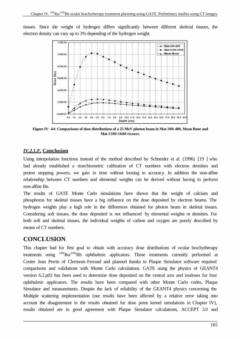
Chapter IV. 106Ru/106Rh ocular brachytherapy treatment planning using GATE. Preliminary studies using CT images.
165
tissues. Since the weight of hydrogen differs significantly between different skeletal tissues, the electron density can vary up to 3% depending of the hydrogen weight.
Figure IV- 44: Comparisons of dose distributions of a 25 MeV photon beam in Mat-300-400, Mean Bone and Mat-1500-1600 tissues.
IV.2.1.F. Conclusion
Using interpolation functions instead of the method described by Schneider et al. (1996) [19 ] who had already established a stoechiometric calibration of CT numbers with electron densities and proton stopping powers, we gain in time without loosing in accuracy. In addition the non-affine relationship between CT numbers and elemental weights can be derived without having to perform non-affine fits. The results of GATE Monte Carlo simulations have shown that the weight of calcium and phosphorus for skeletal tissues have a big influence on the dose deposited by electron beams. The hydrogen weights play a high role in the differences obtained for photon beam in skeletal tissues. Considering soft tissues, the dose deposited is not influenced by elemental weights or densities. For both soft and skeletal tissues, the individual weights of carbon and oxygen are poorly described by means of CT numbers.
CONCLUSION This chapter had for first goal to obtain with accuracy dose distributions of ocular brachytherapy treatments using 106Ru/106Rh ophthalmic applicators. Those treatments currently performed at Centre Jean Perrin of Clermont-Ferrand and planned thanks to Plaque Simulator software required comparisons and validations with Monte Carlo calculations. GATE using the physics of GEANT4 version 6.2.p02 has been used to determine dose deposited on the central axis and isodoses for four ophthalmic applicators. The results have been compared with other Monte Carlo codes, Plaque Simulator and measurements. Despite the lack of reliability of the GEANT4 physics concerning the Multiple scattering implementation (our results have been affected by a relative error taking into account the disagreement in the results obtained for dose point kernel simulations in Chapter IV), results obtained are in good agreement with Plaque Simulator calculations, ACCEPT 3.0 and

Chapter IV. 106Ru/106Rh ocular brachytherapy treatment planning using GATE. Preliminary studies using CT images.
166
measurements on the central axis of the plaques. The fast and easy method consisting into integrating dose point kernels to obtain isodoses don’t give reliable results near the ophthalmic applicator (distance lower than 1mm) and is in bad agreement with GATE concerning isodoses on the median plan. The second part of this chapter was dedicated to the determination of an accurate correlation between density and atomic composition of human tissues with CT numbers. Thanks to the CIRS phantom 062 we established a stoechiometric calibration of CT numbers with tissue parameters for the CT scan providing images for radiotherapy treatments. This method enabled a better determination of the calcium and phosphorus weights in the bone composition which are responsible for high differences in dose distributions of electron beams.
References [1 ] R. Loevinger, E.M. Japha, G.L. Brownell, in radiation Dosimetry ed. G.L. Hine and G.L.
Brownell, New York; Academic Press, 1956. [2 ] W.G. Cross in Phys. Med. Biol. 18, 611, 1968. [3 ] M.J. Berger, MIRD Suppl. 5 5, 1971. [4 ] W.G. Cross, Can. J. Phys. 45 2021, 1967. [5 ] M.J. Berger, Medical Radionuclides: Radiation dose and effects (AEC Symposium Series
N°20) in ed. R.J. Cloutier, C.L. Edwards, W.S. Snyder, Oak Ridge Conf. 69 p 1212, 1970. [6 ] S. Vynckier and A. Wambersie, “Dosimetry of beta sources in radiotherapy I. The beta point
source dose function”, Phys. Med. Biol., Vol.27, N°11, pp 1339-1347, 1982. [7 ] J. Hokkanen, J. Heikkonen, P. Holmberg, “Theoretical calculations of dose distributions for
beta-ray eye applicators”, Med. Phys. 24 (2), pp 211-213, 1997. [8 ] C.G. Soares, S. Vynckier, H. Järvinen, W.G. Cross, P. Sipilä, D. Flühs, B. Schaeken, F.A.
Mourtada, G.A. Bass and T.T. Williams, “Dosimetry of beta-ray ophthalmic applicators: Comparison of different measurement methods”, Med. Phys. 28 (7), pp 1373-1384, July 2001.
[9 ] M.J. Rivard, B.M. Coursey, L.A. DeWerd, W.F. Hanson, M. Saiful Huq, G.S. Ibbott, M.G. Mitch, R. Nath, J.F. Williamson, “Update of AAPM Task Group No.43 Report: A revised AAPM protocol for brachytherapy dose calculations”, Med. Phys. 31 (3), pp 633-673, March 2004.
[10 ] W.G. Cross, J. Hokkanen, H. Järvinen, F. Mourtada, P. Sipilä, C.G. Soares, S. Vynckier, “Calculation of beta-ray dose distributions from ophthalmic applicators and comparison with measurements in a model eye”, Med. Phys. 28 (7), pp 1385-1396, 2001.
[11 ] G. Taccini, F. Cavagnetto, G. Coscia, S. Garelli and A. Pilot, “The determination of dose characteristics of ruthenium ophthalmic applicators using radiochromic film”, Med. Phys. 24 (12), pp 2034-2037, December 1997.
[12 ] J. Davelaar, D.F. Schaling, L.A. Hennen, J.J. Broerse, “Dosimetry of ruthenium-106 eye applicators”, Med. Phys. 19 (3), pp 691-694, May/June 1992.
[13 ] W. Schneider, T. Bortfeld and W. Schlegel, “Correlation between CT numbers and tissue parameters needed for Monte Carlo simulations of clinical dose distributions”, Phys. Med. Biol. 45, pp 459-478, 2000.
[14 ] R.A. Rutherford, B.R. Pullan and I. Isherwood, “Measurement of effective atomic number and electron density using an EMI scanner”, Neuroradiology 11, pp 15-21, 1976.
[15 ] http://www.cirsinc.com/062_rad.html [16 ] D.R. White, H.Q. Woodard and S.M. Hammond, “Average soft tissue and bone models for use
in radiation dosimetry”, Br.J.Radiol., 60 pp907-913, 1987. [17 ] H.Q. Woodard and D.R. White, “The composition of body tissues”, Br. J.Radiol., 59, pp 1209-
1219, 1986. [18 ] H.E. Johns and J.R. Cunningham, “The Physics of Radiology”, Springfield, IL: Thomas,
1983. [19 ] U. Schneider, E. Pedroni and A. Lomax, „The calibration of CT Hounsfield units for
radiotherapy treatment planning”, Phys. Med. Biol. 41, pp 111-124, 1996.
Chapter V.GATE Applications in a Grid Environment
167
Chapter V.
GATE Applications in a Grid Environment INTRODUCTION In radiotherapy-brachytherapy the goal is to evaluate accurately the absorbed dose in complex phantoms and at interfaces of tissue, where analytic calculations have shown some limits. The main drawback of Monte Carlo simulations is their high computing time. The aim of our research is to reduce the computing time by parallelizing a simulation on geographically distributed processors by benefiting of a grid architecture. The method is based on the parallelization of the Random Number Generator (RNG) used in Monte Carlo simulations. In order to let benefit the praticians and the physicists of the considerable gain in time that could be reached thanks to the distributed calculations, a web portal has been customized for GATE applications, asking the user for all the parameters necessary to launch the simulation and retrieve results. Different tests have been done in order to show first, the reliability of the physical results obtained by concatenation of parallelized output data and secondly the time gained for jobs execution using different modalities of submission and different infrastructure. Requirements and use cases caracterizing GATE applications in a grid environment have been detailed [1 ] in and largely mentioned in the EGEE NA4 deliverables [2 ] [3 ]and application migration report [4 ]. The first part will be dedicated to the method used to parallelize GATE simulations. Multiple computing time tests highlight the efficacy of such submission in a grid infrastructure. In a second part is described the transparent and secure access to the grid developed for GATE users and provided by the GENIUS web portal. Finally a synergy between the supercomputing grid DEISA and the EGEE infrastructure is discussed to run on the both infrastructures GATE simulations.
V.1. PARALLELIZATION OF GATE SIMULATIONS WITHIN EGEE
V.1.1. The installation The Experiment Software Manager (ESM) is the person from an experiment responsible for the installation of new software in the different sites. The ESM must have privileges to install software in a particular area of the CEs. There is dedicated space for each one of the supported VOs. An environmental variable holds the path to that space, for biomed applications, its format is the following: $VO_BIOMED_SW_DIR
Chapter V.GATE Applications on a Grid Environment
168
If a site uses a shared file system for the WNs of its CEs, then the software is installed once in the filesystem, and the jobs that want to use it just need to use the $VO_BIOMED_SW_DIR variable to access the software. The GATE platform installation is not trivial as it depends of a large number of softwares to be executed. GATE is a C++ encoded platform and needs to be compiled with a defined environment before each installation. The installation of GATE platform depends on different requirements: § The operating system:
During the EDG project and at the beginning of the first year of the EGEE project, the operating system supporting the middleware and components of the grid was the Linux Redhat version 7.3 (RH7.3). Since April 2005, the operating system move to the Scientific Linux 3.0 (SL3). GATE installations have to adapt to the operating system changes and compiler versions (gcc 2.96 for RH7.3 and gcc 3.2.3 for SL3).
§ The related softwares: ü The GEANT4 software with the data files for specific physics processes associated
to: the three GATE versions that have been installed on the EDG first and then on the EGEE infrastructure are gate_v1.0.2 compatible with the GEANT4 software version 5.2.p02 on the EDG infrastructure and also on the LCG-2-EGEE-0 infrastructure. The gate_v1.1.0 and gate_v1.2.0 respectively compatible with the 6.2.p02 and 7.0.p01 GEANT4 versions have been installed during the first year of the EGEE project on the SL3 operating system.
ü The CLHEP software, needed for the generation of pseudorandom numbers in the Monte Carlo simulations. (CLHEP-1.8.1.0 compatible with the 6.2.p02 and 7.0.p01 GEANT4 versions)
ü The data analysis softwares such as ROOT, AIDA, etc. The ROOT software [5 ] has been installed to enable the analysis of results (ROOT version 4.03.02 compatible with GEANT4 version 7.0.p01 and GATE version 1.2.0).
ü A visualization interface Mesa5.0.2 enabling the use of OpenGL to check geometry construction and particle’s trajectories during GATE simulations.
§ The declaration of environment variables related to the previous software installations. As the installation of such softwares is not applicable to a grid environment using the usual procedure (generally the execution of a configuration script before a make or a gmake compilation), the choice has been done to create precompiled packages of those softwares using a packaging system available on Redhat distributions and named Redhat Package Manager (RPM). The packages must be created each time the operating system evolves and/or the compiler changes. For the SL3 operating system with the gcc 3.2.3 compiler version, the following packages have been created for the installation of the GATE platform (example is given for GATE-1.2.0 version compatible with the 4.7.0.p01 GEANT4 version):
Package Description GATE-1.2.0-1.i386.rpm GATE version 1.2.0 platform
GATE-geant4-7.0.p01-1.i386.rpm GEANT4 (version 7.0.p01) source code
GATE-geant4-G4EMLOW-2.3-1.noarch.rpm, GEANT4 data files for description of the physic processes.
Chapter V.GATE Applications in a Grid Environment
169
GATE-geant4-PhotonEvaporation-2.0-1.noarch.rpm,
GATE-geant4-RadiativeDecay-3.0-1.noarch.rpm,
GATE-geant4-G4NDL-3.7-1.noarch.rpm
the physic processes.
GATE-CLHEP-1.8.1.0-1.i386.rpm CLHEP version 1.8.1.0 .
GATE-root-4.03.02-1.i386.rpm ROOT version 4.03.02 analysis software.
GATE-Mesa-5.0.2-1.i386.rpm OpenGL visualization
GATE-env-1.2.0-1.noarch.rpm Scripts describing the environment for installations.
Those packages have been installed on each of the CEs hosting the biomed VO on the EGEE infrastructure. The packages have been installed by the software administrator by sending a job which create a gate/ repository under the $VO_BIOMED_SW_DIR area and perform the RPMs installation. After each installation of GATE on a site, a test-job is sent on the site to check the well-running of the platform with the ROOT analysis. Finally, the software must be published in the Information System (IS), so that the jobs requesting for a particular piece of software can be directed to the appropriate CE. For that purpose, a tag is added to the GlueHostApplicationSoftwareRunTimeEnvironment attribute of the IS using the following perl command line in a job for the LCG-2 middleware: perl /opt/lcg/bin/lcg-ManageVOTag –host <CE_HOST> -vo biomed --add -tag VO-biomed-GATE-1.2.0-1
At the date of the 2005, GATE version 1.1.0 compatible with the GEANT4 version 6.2.p02 have been installed on each site hosting the biomed VO (see Chapter II. for the biomed CEs resources).
V.1.2. The parallelisation of GATE simulations and tests of submission to a grid environment
V.1.2.A. Introduction
Monte Carlo simulations use random numbers responsible for the name given to this technique which was introduced during the development of atomic energy in the post World War II era. Even though the cost of computing resources is continually decreasing thereby facilitating consequent calculations, Monte Carlo simulations can’t currently be used for clinical treatments planning for which the computing time remains too high on a single machine. So, there is a real interest for parallel and distributed Monte Carlo simulations in order to provide very accurate studies in medical physics. A Random Number Generator (RNG) used in Monte Carlo calculations generally involves a recursive deterministic algorithm to produce a sequence of pseudo random numbers. Because particles ranges in matter are independent of each other, parallel simulations are produced by partitioning the random sequence into independent streams. Then, we present a method to display the simulations on geographically distributed processors using a grid environment. The final outcome of the application is to provide a web portal to launch simulations in parallel.
Chapter V.GATE Applications on a Grid Environment
170
V.1.2.B. The Random Number Generator (RNG) in Monte Carlo simulations
The computing time of a Monte Carlo simulation depends on different parameters: the number of particles generated during a simulation, the medium where particles interactions occur. Depending on the type of material filling the medium and the type of particles generated, the number of physical interactions can vary. The number of calls to the RNG is consequently dependant on these parameters [6 ]. Even if the computing time of a simulation depends also on the construction of the geometry, physical processes used, etc.., the parallelization of such parameters appears to be tricky and won’t be tackled in this study. Each Monte Carlo simulation uses a sequence of random numbers to reproduce the probability of the physical interactions in matter. The more numerous the interactions in a medium are, the longer the sequence of random numbers generated for the simulation is. A simple way to reduce the execution time of a Monte Carlo simulation used in physical experiments, is to sub-divide a long or a very long simulation into little ones by indexing to each simulation a sub-sequence of random numbers obtained by partitioning a long sequence of random numbers. Sub-sequences have to be independent and as we explained before this method is valid only because the particles emitted in simulations are not dependant on each other.
V.1.2.B.1. Principle
Physicists need very good random number generators for Monte Carlo calculations. Random numbers generators can be classified according to the three types of random numbers [6 ][7 ]: § Truly random numbers are unpredictable, they are not generated by a determinist process,
and must be produced by a random physical process such as radioactive decay. § Pseudorandom numbers are produced in the computer by a simple numerical algorithm, and
are therefore not truly random. § Quasirandom numbers are introduced to improve the accuracy of Monte Carlo integration;
these numbers are not independent and thus cannot be used generally. Statistically sound random number sequences usually satisfy a set of requirements that can be divided into three main classes: randomness, practical qualities and performance [8 ]. In practice, all the requirements are not easily achieved concurrently since some of them are antagonistic. Monte Carlo simulations are very sensitive to the statistical soundness of pseudorandom number generators and scientists usually use high quality generators. In our study, we use a Very Long Period (VLP) shuffled pseudo random number generator; the general technique in order to run this type of generator is: § The set up of an internal table, containing a large number of seeds (typically between 10 and
a few hundreds), and the values of a few indices (typically two) pointing to seeds in the table, are also initialized.
§ The generation of pseudorandom number by combining only those seeds corresponding to the current values of the indices.
§ The update of the seeds just used and the pseudorandom generation of new indices to point to other seeds.
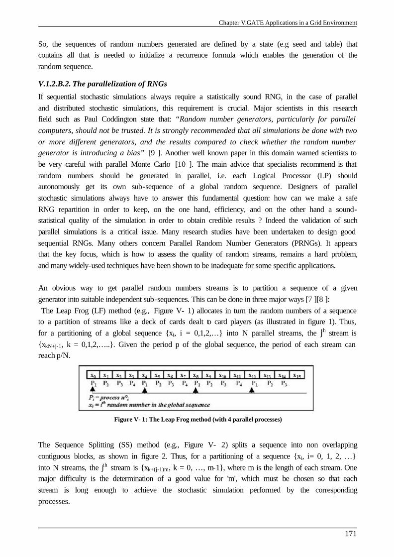
Chapter V.GATE Applications in a Grid Environment
171
So, the sequences of random numbers generated are defined by a state (e.g seed and table) that contains all that is needed to initialize a recurrence formula which enables the generation of the random sequence.
V.1.2.B.2. The parallelization of RNGs
If sequential stochastic simulations always require a statistically sound RNG, in the case of parallel and distributed stochastic simulations, this requirement is crucial. Major scientists in this research field such as Paul Coddington state that: “Random number generators, particularly for parallel computers, should not be trusted. It is strongly recommended that all simulations be done with two or more different generators, and the results compared to check whether the random number generator is introducing a bias” [9 ]. Another well known paper in this domain warned scientists to be very careful with parallel Monte Carlo [10 ]. The main advice that specialists recommend is that random numbers should be generated in parallel, i.e. each Logical Processor (LP) should autonomously get its own sub-sequence of a global random sequence. Designers of parallel stochastic simulations always have to answer this fundamental question: how can we make a safe RNG repartition in order to keep, on the one hand, efficiency, and on the other hand a sound-statistical quality of the simulation in order to obtain credible results ? Indeed the validation of such parallel simulations is a critical issue. Many research studies have been undertaken to design good sequential RNGs. Many others concern Parallel Random Number Generators (PRNGs). It appears that the key focus, which is how to assess the quality of random streams, remains a hard problem, and many widely-used techniques have been shown to be inadequate for some specific applications. An obvious way to get parallel random numbers streams is to partition a sequence of a given generator into suitable independent sub-sequences. This can be done in three major ways [7 ][8 ]: The Leap Frog (LF) method (e.g., Figure V- 1) allocates in turn the random numbers of a sequence to a partition of streams like a deck of cards dealt to card players (as illustrated in figure 1). Thus, for a partitioning of a global sequence {xi, i = 0,1,2,…} into N parallel streams, the jth stream is {xkN+j-1, k = 0,1,2,…..}. Given the period p of the global sequence, the period of each stream can reach p/N.
Figure V- 1: The Leap Frog method (with 4 parallel processes)
The Sequence Splitting (SS) method (e.g., Figure V- 2) splits a sequence into non overlapping contiguous blocks, as shown in figure 2. Thus, for a partitioning of a sequence {xi, i= 0, 1, 2, …} into N streams, the jth stream is {xk+(j-1)m, k = 0, …, m-1}, where m is the length of each stream. One major difficulty is the determination of a good value for 'm', which must be chosen so that each stream is long enough to achieve the stochastic simulation performed by the corresponding processes.
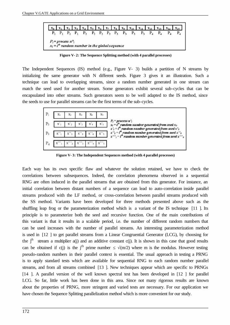
Chapter V.GATE Applications on a Grid Environment
172
Figure V- 2: The Sequence Splitting method (with 4 parallel processes)
The Independent Sequences (IS) method (e.g., Figure V- 3) builds a partition of N streams by initializing the same generator with N different seeds. Figure 3 gives it an illustration. Such a technique can lead to overlapping streams, since a random number generated in one stream can match the seed used for another stream. Some generators exhibit several sub-cycles that can be encapsulated into other streams. Such generators seem to be well adapted to the IS method, since the seeds to use for parallel streams can be the first terms of the sub-cycles.
Figure V- 3: The Independent Sequences method (with 4 parallel processes)
Each way has its own specific flaw and whatever the solution retained, we have to check the correlations between subsequences. Indeed, the correlation phenomena observed in a sequential RNG are often induced in the parallel streams that are obtained from this generator. For instance, an initial correlation between distant numbers of a sequence can lead to auto-correlation inside parallel streams produced with the LF method, or cross-correlation between parallel streams produced with the SS method. Variants have been developed for three methods presented above such as the shuffling leap frog or the parameterization method which is a variant of the IS technique [11 ]. Its principle is to parameterize both the seed and recursive function. One of the main contributions of this variant is that it results in a scalable period, i.e. the number of different random numbers that can be used increases with the number of parallel streams. An interesting parameterization method is used in [12 ] to get parallel streams from a Linear Congruential Generator (LCG), by choosing for the jth stream a multiplier a(j) and an additive constant c(j). It is shown in this case that good results can be obtained if c(j) is the jth prime number ≤ √(m/2) where m is the modulus. However testing pseudo-random numbers in their parallel context is essential. The usual approach in testing a PRNG is to apply standard tests which are available for sequential RNG to each random number parallel streams, and from all streams combined [13 ]. New techniques appear which are specific to PRNGs [14 ]. A parallel version of the well known spectral test has been developed in [12 ] for parallel LCG. So far, little work has been done in this area. Since not many rigorous results are known about the properties of PRNG, more stringent and varied tests are necessary. For our application we have chosen the Sequence Splitting parallelization method which is more convenient for our study.
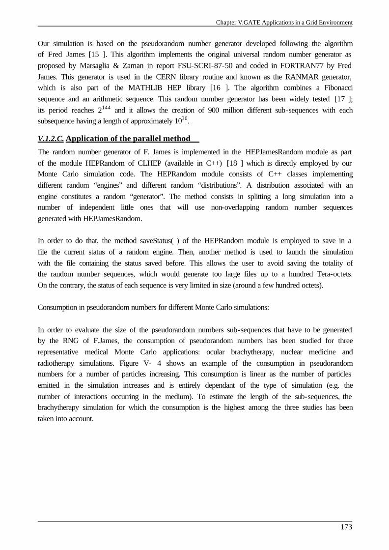
Chapter V.GATE Applications in a Grid Environment
173
Our simulation is based on the pseudorandom number generator developed following the algorithm of Fred James [15 ]. This algorithm implements the original universal random number generator as proposed by Marsaglia & Zaman in report FSU-SCRI-87-50 and coded in FORTRAN77 by Fred James. This generator is used in the CERN library routine and known as the RANMAR generator, which is also part of the MATHLIB HEP library [16 ]. The algorithm combines a Fibonacci sequence and an arithmetic sequence. This random number generator has been widely tested [17 ]; its period reaches 2144 and it allows the creation of 900 million different sub-sequences with each subsequence having a length of approximately 1030.
V.1.2.C. Application of the parallel method
The random number generator of F. James is implemented in the HEPJamesRandom module as part of the module HEPRandom of CLHEP (available in C++) [18 ] which is directly employed by our Monte Carlo simulation code. The HEPRandom module consists of C++ classes implementing different random “engines” and different random “distributions”. A distribution associated with an engine constitutes a random “generator”. The method consists in splitting a long simulation into a number of independent little ones that will use non-overlapping random number sequences generated with HEPJamesRandom. In order to do that, the method saveStatus( ) of the HEPRandom module is employed to save in a file the current status of a random engine. Then, another method is used to launch the simulation with the file containing the status saved before. This allows the user to avoid saving the totality of the random number sequences, which would generate too large files up to a hundred Tera-octets. On the contrary, the status of each sequence is very limited in size (around a few hundred octets). Consumption in pseudorandom numbers for different Monte Carlo simulations: In order to evaluate the size of the pseudorandom numbers sub-sequences that have to be generated by the RNG of F.James, the consumption of pseudorandom numbers has been studied for three representative medical Monte Carlo applications: ocular brachytherapy, nuclear medicine and radiotherapy simulations. Figure V- 4 shows an example of the consumption in pseudorandom numbers for a number of particles increasing. This consumption is linear as the number of particles emitted in the simulation increases and is entirely dependant of the type of simulation (e.g. the number of interactions occurring in the medium). To estimate the length of the sub-sequences, the brachytherapy simulation for which the consumption is the highest among the three studies has been taken into account.
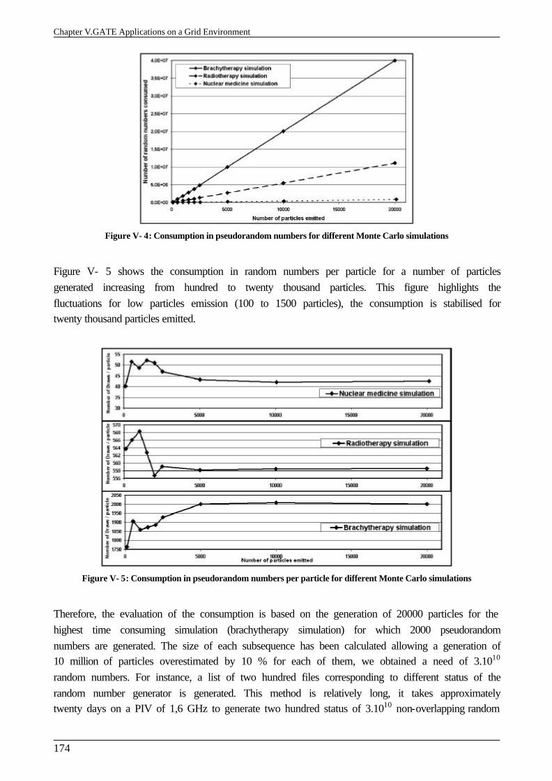
Chapter V.GATE Applications on a Grid Environment
174
Figure V- 4: Consumption in pseudorandom numbers for different Monte Carlo simulations
Figure V- 5 shows the consumption in random numbers per particle for a number of particles generated increasing from hundred to twenty thousand particles. This figure highlights the fluctuations for low particles emission (100 to 1500 particles), the consumption is stabilised for twenty thousand particles emitted.
Figure V- 5: Consumption in pseudorandom numbers per particle for different Monte Carlo simulations
Therefore, the evaluation of the consumption is based on the generation of 20000 particles for the highest time consuming simulation (brachytherapy simulation) for which 2000 pseudorandom numbers are generated. The size of each subsequence has been calculated allowing a generation of 10 million of particles overestimated by 10 % for each of them, we obtained a need of 3.1010 random numbers. For instance, a list of two hundred files corresponding to different status of the random number generator is generated. This method is relatively long, it takes approximately twenty days on a PIV of 1,6 GHz to generate two hundred status of 3.1010 non-overlapping random
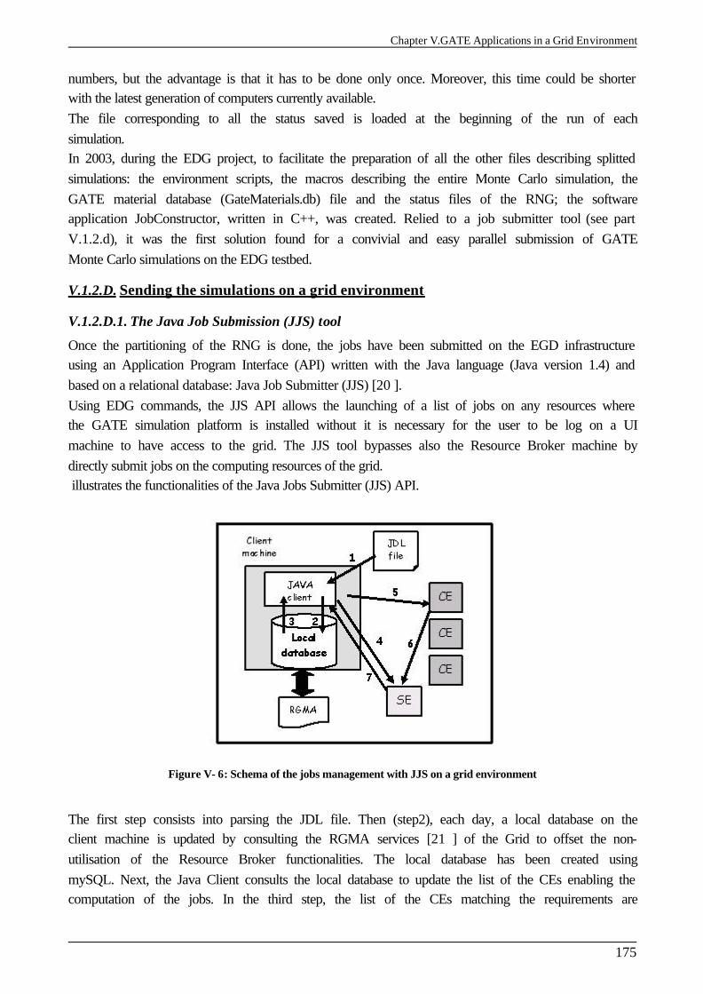
Chapter V.GATE Applications in a Grid Environment
175
numbers, but the advantage is that it has to be done only once. Moreover, this time could be shorter with the latest generation of computers currently available. The file corresponding to all the status saved is loaded at the beginning of the run of each simulation. In 2003, during the EDG project, to facilitate the preparation of all the other files describing splitted simulations: the environment scripts, the macros describing the entire Monte Carlo simulation, the GATE material database (GateMaterials.db) file and the status files of the RNG; the software application JobConstructor, written in C++, was created. Relied to a job submitter tool (see part V.1.2.d), it was the first solution found for a convivial and easy parallel submission of GATE Monte Carlo simulations on the EDG testbed.
V.1.2.D. Sending the simulations on a grid environment
V.1.2.D.1. The Java Job Submission (JJS) tool
Once the partitioning of the RNG is done, the jobs have been submitted on the EGD infrastructure using an Application Program Interface (API) written with the Java language (Java version 1.4) and based on a relational database: Java Job Submitter (JJS) [20 ]. Using EDG commands, the JJS API allows the launching of a list of jobs on any resources where the GATE simulation platform is installed without it is necessary for the user to be log on a UI machine to have access to the grid. The JJS tool bypasses also the Resource Broker machine by directly submit jobs on the computing resources of the grid. illustrates the functionalities of the Java Jobs Submitter (JJS) API.
Figure V- 6: Schema of the jobs management with JJS on a grid environment
The first step consists into parsing the JDL file. Then (step2), each day, a local database on the client machine is updated by consulting the RGMA services [21 ] of the Grid to offset the non-utilisation of the Resource Broker functionalities. The local database has been created using mySQL. Next, the Java Client consults the local database to update the list of the CEs enabling the computation of the jobs. In the third step, the list of the CEs matching the requirements are
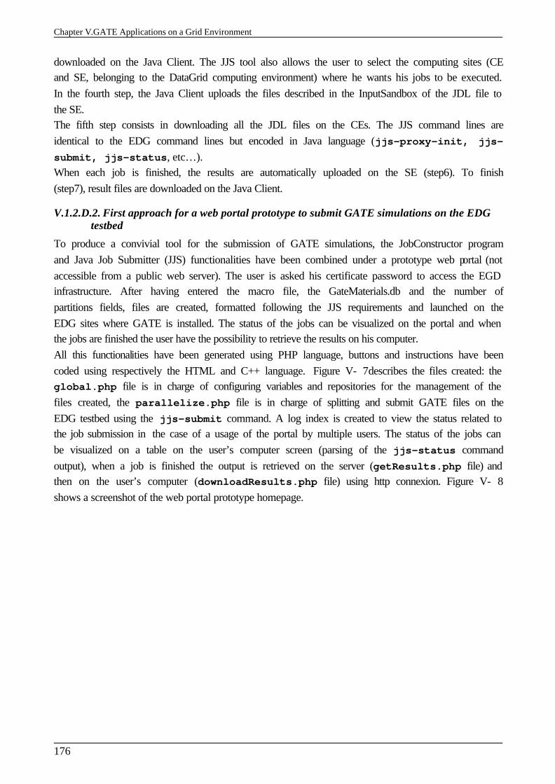
Chapter V.GATE Applications on a Grid Environment
176
downloaded on the Java Client. The JJS tool also allows the user to select the computing sites (CE and SE, belonging to the DataGrid computing environment) where he wants his jobs to be executed. In the fourth step, the Java Client uploads the files described in the InputSandbox of the JDL file to the SE. The fifth step consists in downloading all the JDL files on the CEs. The JJS command lines are identical to the EDG command lines but encoded in Java language (jjs-proxy-init, jjs-submit, jjs-status, etc…). When each job is finished, the results are automatically uploaded on the SE (step6). To finish (step7), result files are downloaded on the Java Client.
V.1.2.D.2. First approach for a web portal prototype to submit GATE simulations on the EDG testbed
To produce a convivial tool for the submission of GATE simulations, the JobConstructor program and Java Job Submitter (JJS) functionalities have been combined under a prototype web portal (not accessible from a public web server). The user is asked his certificate password to access the EGD infrastructure. After having entered the macro file, the GateMaterials.db and the number of partitions fields, files are created, formatted following the JJS requirements and launched on the EDG sites where GATE is installed. The status of the jobs can be visualized on the portal and when the jobs are finished the user have the possibility to retrieve the results on his computer. All this functionalities have been generated using PHP language, buttons and instructions have been coded using respectively the HTML and C++ language. Figure V- 7describes the files created: the global.php file is in charge of configuring variables and repositories for the management of the files created, the parallelize.php file is in charge of splitting and submit GATE files on the EDG testbed using the jjs-submit command. A log index is created to view the status related to the job submission in the case of a usage of the portal by multiple users. The status of the jobs can be visualized on a table on the user’s computer screen (parsing of the jjs-status command output), when a job is finished the output is retrieved on the server (getResults.php file) and then on the user’s computer (downloadResults.php file) using http connexion. Figure V- 8 shows a screenshot of the web portal prototype homepage.
Chapter V.GATE Applications in a Grid Environment
177
Figure V- 7: Prototype web portal algorithmic schema.
Figure V- 8: A web portal prototype for the parallelisation and submission of GATE simulations on the EDG testbed.
V.1.2.E. Results
All the calculations were distributed between the site of CC-IN2P3 worker nodes in Lyon and the site of Laboratoire de Physique Corpusculaire (LPC) in Clermont-Ferrand, on the EDG testbed. At this time (July 2003), CC-IN2P3 provided 200 dual-processors mixed in PIII 750 MHz, 1GHz and PIV at 1,4 GHz ; and the LPC provided 4 PIII mono-processors at 933 MHz. The distribution of jobs was managed by a batch manager developed at CC-IN2P3 named BQS (Batch Queuing System) and by PBS (Personal Batch System) at LPC. This management takes into account the CPU time specified by the user for his jobs.
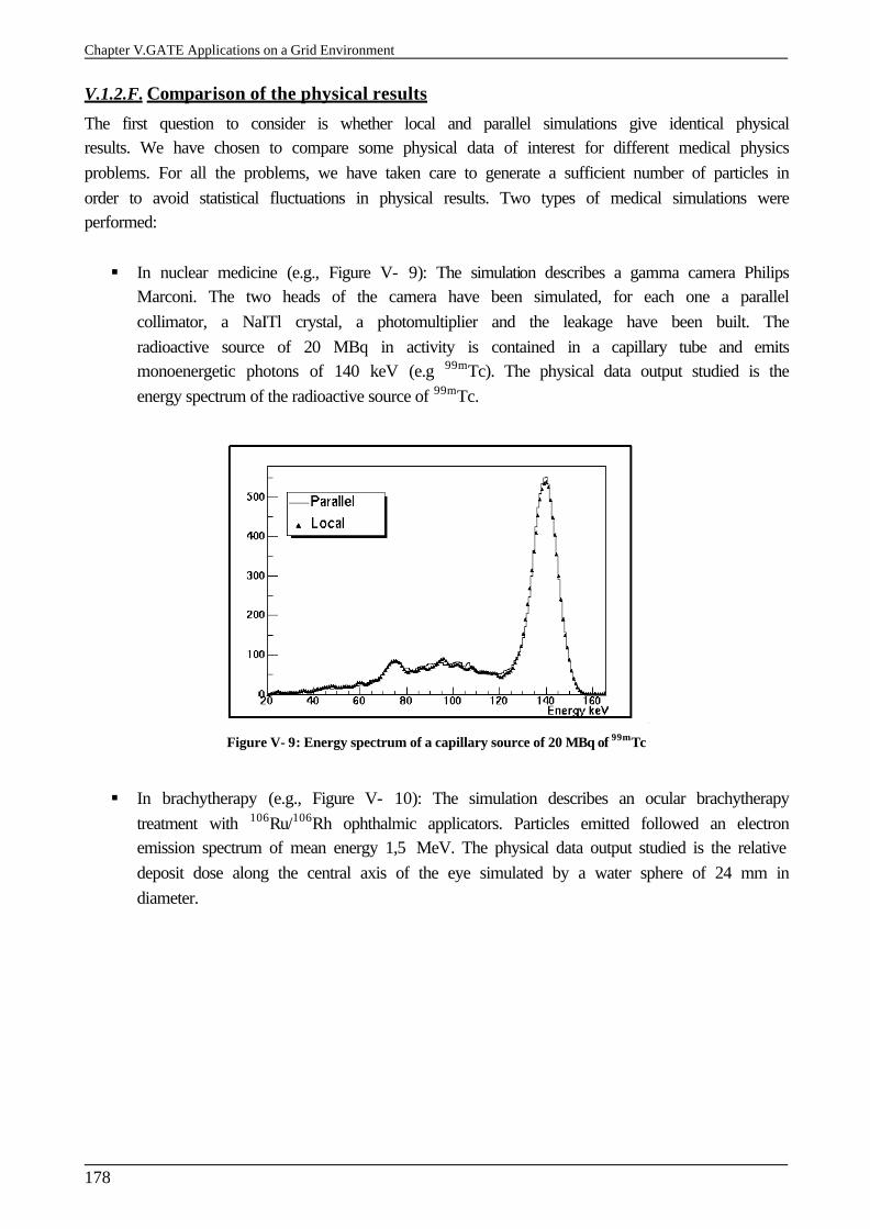
Chapter V.GATE Applications on a Grid Environment
178
V.1.2.F. Comparison of the physical results
The first question to consider is whether local and parallel simulations give identical physical results. We have chosen to compare some physical data of interest for different medical physics problems. For all the problems, we have taken care to generate a sufficient number of particles in order to avoid statistical fluctuations in physical results. Two types of medical simulations were performed: § In nuclear medicine (e.g., Figure V- 9): The simulation describes a gamma camera Philips
Marconi. The two heads of the camera have been simulated, for each one a parallel collimator, a NaITl crystal, a photomultiplier and the leakage have been built. The radioactive source of 20 MBq in activity is contained in a capillary tube and emits monoenergetic photons of 140 keV (e.g 99mTc). The physical data output studied is the energy spectrum of the radioactive source of 99mTc.
Figure V- 9: Energy spectrum of a capillary source of 20 MBq of 99mTc
§ In brachytherapy (e.g., Figure V- 10): The simulation describes an ocular brachytherapy
treatment with 106Ru/106Rh ophthalmic applicators. Particles emitted followed an electron emission spectrum of mean energy 1,5 MeV. The physical data output studied is the relative deposit dose along the central axis of the eye simulated by a water sphere of 24 mm in diameter.
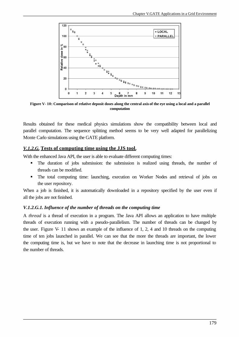
Chapter V.GATE Applications in a Grid Environment
179
Figure V- 10: Comparison of relative deposit doses along the central axis of the eye using a local and a parallel computation
Results obtained for these medical physics simulations show the compatibility between local and parallel computation. The sequence splitting method seems to be very well adapted for parallelizing Monte Carlo simulations using the GATE platform.
V.1.2.G. Tests of computing time using the JJS tool.
With the enhanced Java API, the user is able to evaluate different computing times: § The duration of jobs submission: the submission is realized using threads, the number of
threads can be modified. § The total computing time: launching, execution on Worker Nodes and retrieval of jobs on
the user repository. When a job is finished, it is automatically downloaded in a repository specified by the user even if all the jobs are not finished.
V.1.2.G.1. Influence of the number of threads on the computing time
A thread is a thread of execution in a program. The Java API allows an application to have multiple threads of execution running with a pseudo-parallelism. The number of threads can be changed by the user. Figure V- 11 shows an example of the influence of 1, 2, 4 and 10 threads on the computing time of ten jobs launched in parallel. We can see that the more the threads are important, the lower the computing time is, but we have to note that the decrease in launching time is not proportional to the number of threads.
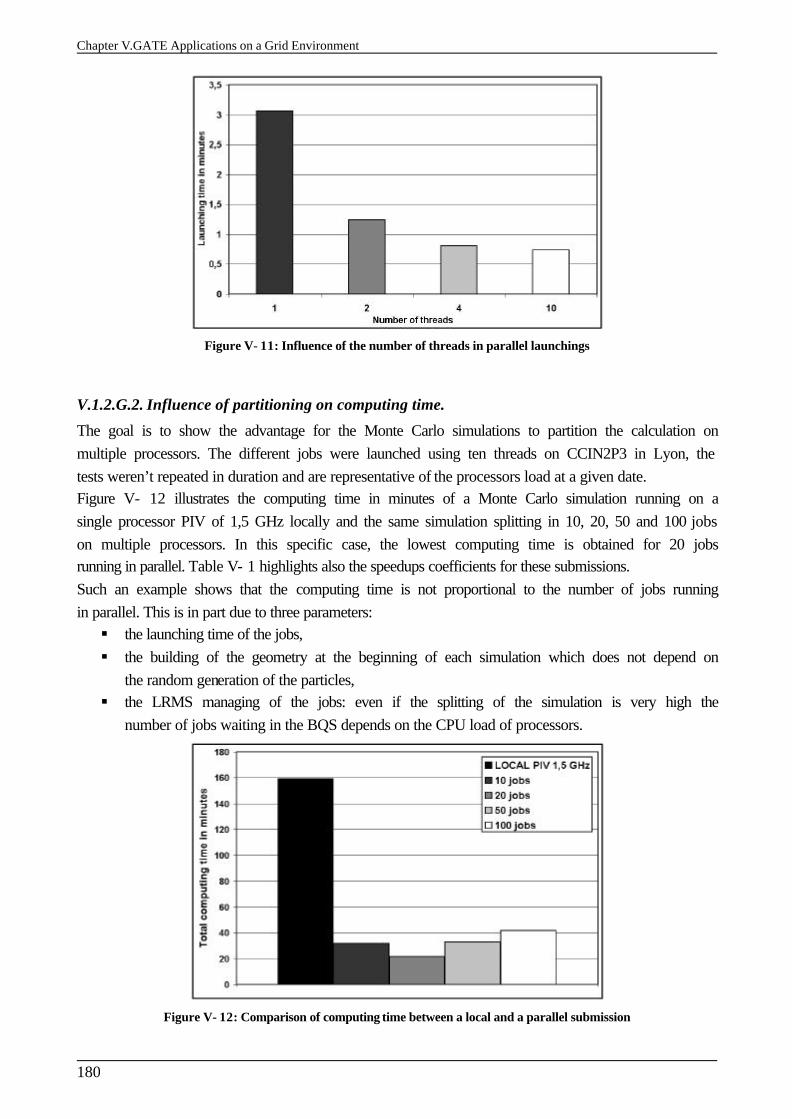
Chapter V.GATE Applications on a Grid Environment
180
Figure V- 11: Influence of the number of threads in parallel launchings
V.1.2.G.2. Influence of partitioning on computing time.
The goal is to show the advantage for the Monte Carlo simulations to partition the calculation on multiple processors. The different jobs were launched using ten threads on CCIN2P3 in Lyon, the tests weren’t repeated in duration and are representative of the processors load at a given date. Figure V- 12 illustrates the computing time in minutes of a Monte Carlo simulation running on a single processor PIV of 1,5 GHz locally and the same simulation splitting in 10, 20, 50 and 100 jobs on multiple processors. In this specific case, the lowest computing time is obtained for 20 jobs running in parallel. Table V- 1 highlights also the speedups coefficients for these submissions. Such an example shows that the computing time is not proportional to the number of jobs running in parallel. This is in part due to three parameters: § the launching time of the jobs, § the building of the geometry at the beginning of each simulation which does not depend on
the random generation of the particles, § the LRMS managing of the jobs: even if the splitting of the simulation is very high the
number of jobs waiting in the BQS depends on the CPU load of processors.
Figure V- 12: Comparison of computing time between a local and a parallel submission
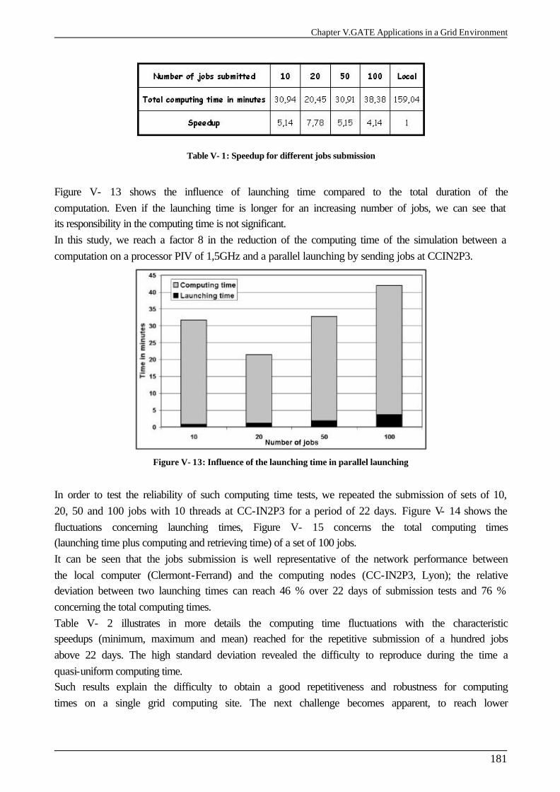
Chapter V.GATE Applications in a Grid Environment
181
Table V- 1: Speedup for different jobs submission
Figure V- 13 shows the influence of launching time compared to the total duration of the computation. Even if the launching time is longer for an increasing number of jobs, we can see that its responsibility in the computing time is not significant. In this study, we reach a factor 8 in the reduction of the computing time of the simulation between a computation on a processor PIV of 1,5GHz and a parallel launching by sending jobs at CCIN2P3.
Figure V- 13: Influence of the launching time in parallel launching
In order to test the reliability of such computing time tests, we repeated the submission of sets of 10, 20, 50 and 100 jobs with 10 threads at CC-IN2P3 for a period of 22 days. Figure V- 14 shows the fluctuations concerning launching times, Figure V- 15 concerns the total computing times (launching time plus computing and retrieving time) of a set of 100 jobs. It can be seen that the jobs submission is well representative of the network performance between the local computer (Clermont-Ferrand) and the computing nodes (CC-IN2P3, Lyon); the relative deviation between two launching times can reach 46 % over 22 days of submission tests and 76 % concerning the total computing times. Table V- 2 illustrates in more details the computing time fluctuations with the characteristic speedups (minimum, maximum and mean) reached for the repetitive submission of a hundred jobs above 22 days. The high standard deviation revealed the difficulty to reproduce during the time a quasi-uniform computing time. Such results explain the difficulty to obtain a good repetitiveness and robustness for computing times on a single grid computing site. The next challenge becomes apparent, to reach lower
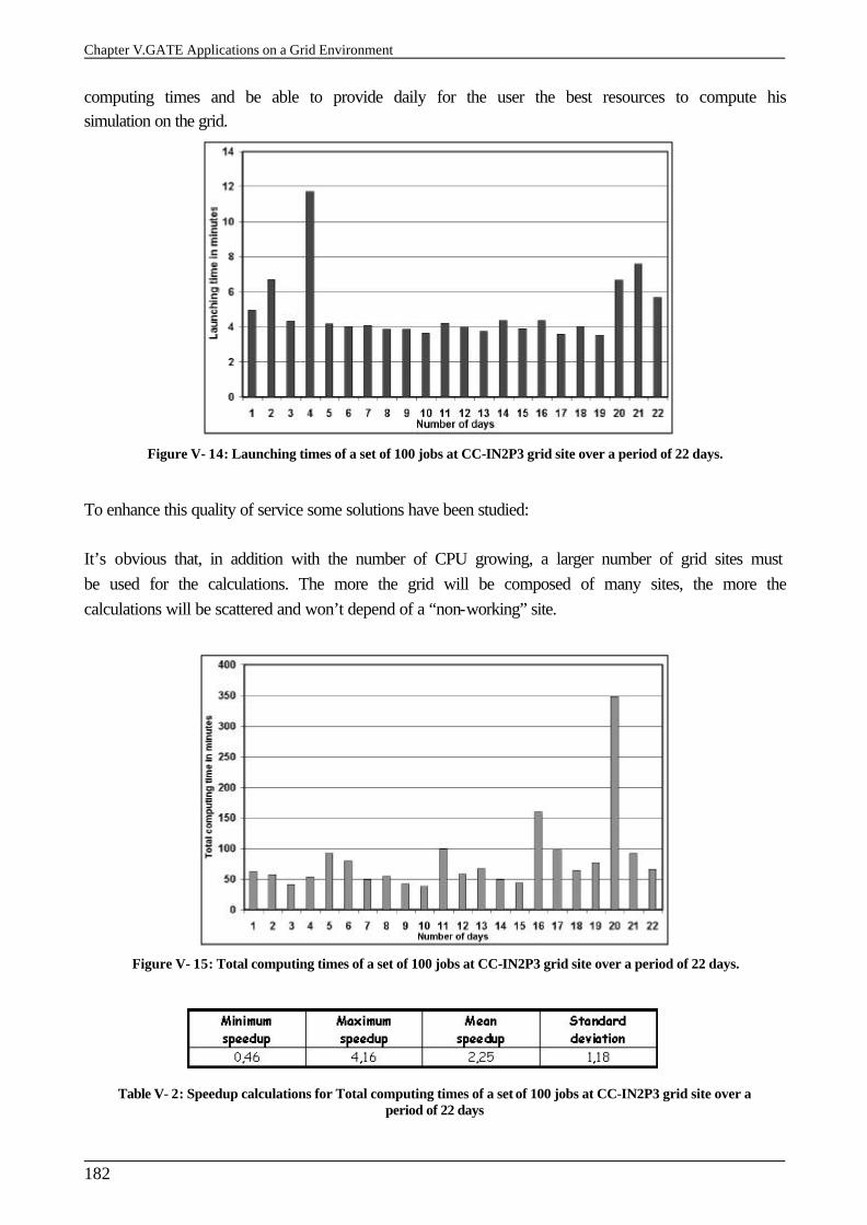
Chapter V.GATE Applications on a Grid Environment
182
computing times and be able to provide daily for the user the best resources to compute his simulation on the grid.
Figure V- 14: Launching times of a set of 100 jobs at CC-IN2P3 grid site over a period of 22 days.
To enhance this quality of service some solutions have been studied: It’s obvious that, in addition with the number of CPU growing, a larger number of grid sites must be used for the calculations. The more the grid will be composed of many sites, the more the calculations will be scattered and won’t depend of a “non-working” site.
Figure V- 15: Total computing times of a set of 100 jobs at CC-IN2P3 grid site over a period of 22 days.
Table V- 2: Speedup calculations for Total computing times of a set of 100 jobs at CC-IN2P3 grid site over a period of 22 days
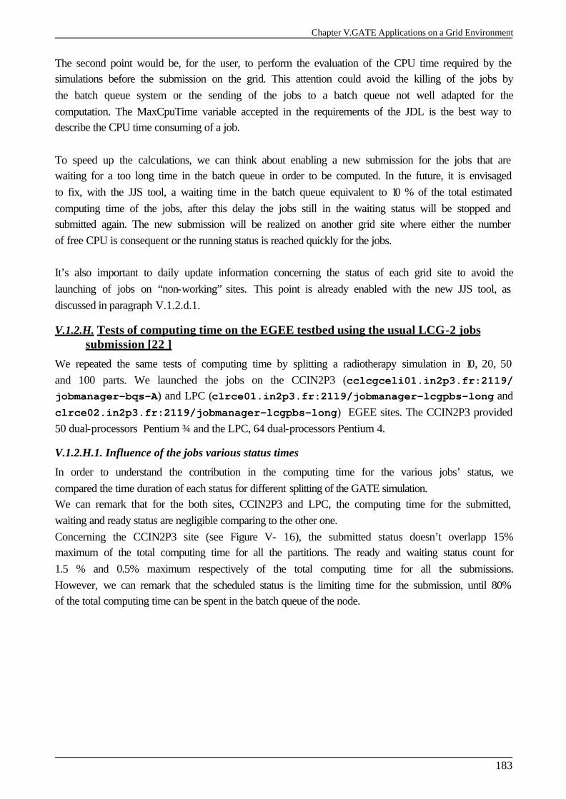
Chapter V.GATE Applications on a Grid Environment
183
The second point would be, for the user, to perform the evaluation of the CPU time required by the simulations before the submission on the grid. This attention could avoid the killing of the jobs by the batch queue system or the sending of the jobs to a batch queue not well adapted for the computation. The MaxCpuTime variable accepted in the requirements of the JDL is the best way to describe the CPU time consuming of a job. To speed up the calculations, we can think about enabling a new submission for the jobs that are waiting for a too long time in the batch queue in order to be computed. In the future, it is envisaged to fix, with the JJS tool, a waiting time in the batch queue equivalent to 10 % of the total estimated computing time of the jobs, after this delay the jobs still in the waiting status will be stopped and submitted again. The new submission will be realized on another grid site where either the number of free CPU is consequent or the running status is reached quickly for the jobs. It’s also important to daily update information concerning the status of each grid site to avoid the launching of jobs on “non-working” sites. This point is already enabled with the new JJS tool, as discussed in paragraph V.1.2.d.1.
V.1.2.H. Tests of computing time on the EGEE testbed using the usual LCG-2 jobs submission [22 ]
We repeated the same tests of computing time by splitting a radiotherapy simulation in 10, 20, 50 and 100 parts. We launched the jobs on the CCIN2P3 (cclcgceli01.in2p3.fr:2119/ jobmanager-bqs-A) and LPC (clrce01.in2p3.fr:2119/jobmanager-lcgpbs-long and clrce02.in2p3.fr:2119/jobmanager-lcgpbs-long) EGEE sites. The CCIN2P3 provided 50 dual-processors Pentium ¾ and the LPC, 64 dual-processors Pentium 4.
V.1.2.H.1. Influence of the jobs various status times
In order to understand the contribution in the computing time for the various jobs’ status, we compared the time duration of each status for different splitting of the GATE simulation. We can remark that for the both sites, CCIN2P3 and LPC, the computing time for the submitted, waiting and ready status are negligible comparing to the other one. Concerning the CCIN2P3 site (see Figure V- 16), the submitted status doesn’t overlapp 15% maximum of the total computing time for all the partitions. The ready and waiting status count for 1.5 % and 0.5% maximum respectively of the total computing time for all the submissions. However, we can remark that the scheduled status is the limiting time for the submission, until 80% of the total computing time can be spent in the batch queue of the node.
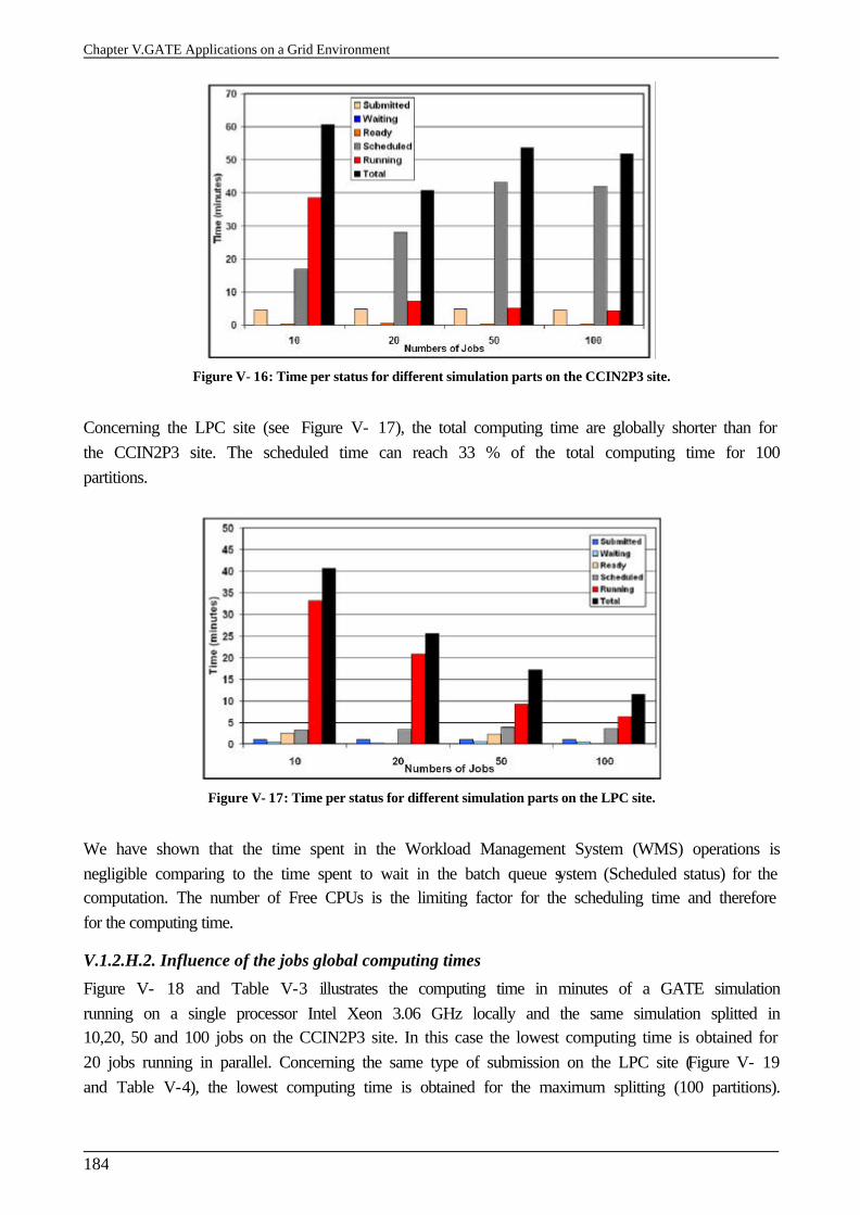
Chapter V.GATE Applications on a Grid Environment
184
Figure V- 16: Time per status for different simulation parts on the CCIN2P3 site.
Concerning the LPC site (see Figure V- 17), the total computing time are globally shorter than for the CCIN2P3 site. The scheduled time can reach 33 % of the total computing time for 100 partitions.
Figure V- 17: Time per status for different simulation parts on the LPC site.
We have shown that the time spent in the Workload Management System (WMS) operations is negligible comparing to the time spent to wait in the batch queue system (Scheduled status) for the computation. The number of Free CPUs is the limiting factor for the scheduling time and therefore for the computing time.
V.1.2.H.2. Influence of the jobs global computing times
Figure V- 18 and Table V-3 illustrates the computing time in minutes of a GATE simulation running on a single processor Intel Xeon 3.06 GHz locally and the same simulation splitted in 10,20, 50 and 100 jobs on the CCIN2P3 site. In this case the lowest computing time is obtained for 20 jobs running in parallel. Concerning the same type of submission on the LPC site (Figure V- 19 and Table V-4), the lowest computing time is obtained for the maximum splitting (100 partitions).
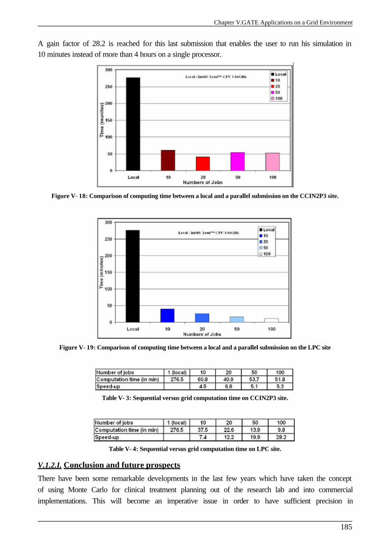
Chapter V.GATE Applications on a Grid Environment
185
A gain factor of 28.2 is reached for this last submission that enables the user to run his simulation in 10 minutes instead of more than 4 hours on a single processor.
Figure V- 18: Comparison of computing time between a local and a parallel submission on the CCIN2P3 site.
Figure V- 19: Comparison of computing time between a local and a parallel submission on the LPC site
Table V- 3: Sequential versus grid computation time on CCIN2P3 site.
Table V- 4: Sequential versus grid computation time on LPC site.
V.1.2.I. Conclusion and future prospects
There have been some remarkable developments in the last few years which have taken the concept of using Monte Carlo for clinical treatment planning out of the research lab and into commercial implementations. This will become an imperative issue in order to have sufficient precision in

Chapter V.GATE Applications on a Grid Environment
186
cancer treatments. However, the computing time using Monte Carlo calculations must stay comparable to what it is currently with analytical calculations. It can be seen that the parallelization of Monte Carlo simulations by splitting pseudorandom numbers generator sequences into a multitude of streams is a simple, rigorous and generic method (e.g it can be applied for each Monte Carlo codes used in physics with a pseudorandom number generator). The comparison between a local and a parallel computation of some physical results of interest shows that the output data stay unchanged and therefore validate the parallelization method used. The gain in computing time obtained by splitting the simulations is encouraging. Even if a parallel launching using a consequent number of threads speeds up the computing time, it is not responsible for the time consumption. The construction of the geometry in a Monte Carlo simulation and especially the CPU load of processors are the limiting factors in reducing time consumption. Up to now, 1000 status of the pseudorandom numbers generator have been generated and allow the user to parallelize a simulation in 1000 jobs. With the CPU resources increasing in future grid projects, we can expect to reach up to a factor 1000 in order to reduce time consumption. Thereafter, the development of a convivial tool to split, launch and retrieve Monte Carlo simulations on a grid environment using a web portal is the answer to the parallelization of Monte Carlo simulations in physics.
V.2. GATE APPLICATIONS ON THE GENIUS WEB PORTAL At the beginning of 2002, the Italian INFN Grid Project [23 ] started the GENIUS Portal Project in conjunction with the Italian web company NICE srl [24 ]. The goal of this collaboration was to create a web portal that would overcome all the difficulties related to the complex command lines interfaces (CLI) and the job description language (JDL) that a user encounters when he has to submit his application in a grid environment. We will describe first the architecture and implementation of the portal, the services offered and to finish the work realized (since April 2004) to customize the portal in order to allow transparent GATE jobs submission and management on the EGEE-LCG2 infrastructure.
V.2.1. Architecture and implementation of the portal The GENIUS [25 ] [26 ] web portal is carried out on the top of the middleware services of the EGEE infrastructure (and before the EU DataGrid Project). The layout of the portal can be described by a three-tier architecture model, see Figure V- 20. From the user’s workstation (the client, on the right top on the figure), a web browser is running (Internet Explorer and Mozilla are the two web browsers compatible with GENIUS) and enable the access to the EGEE grid infrastructure by having access to the User Interface. The EGEE User interface (UI) machine (the server, on the left side of the figure) runs the Apache web server, the Java/XML framework EngineFrame developed by NICE and GENIUS itself. From the User interface via the portal the user has access to the remote resources: the Grid.
Chapter V.GATE Applications on a Grid Environment
187
Figure V- 20: Three-tier architecture of the GENIUS portal
Using those services, the user can interact with files on the UI and from there the user can launch jobs to the grid and manage the data belonging to his VO membership. In order to guarantee a secured access to the grid, GENIUS has been implemented with a multi-layered security infrastructure: § All web transactions are executed under the Secure Socket Layer (SSL) via HTTPS § The user has to obtain an account on a UI machine of the grid and be part of a VO. § At each time a user wants to interact with files on the UI machine, he is prompted for the
username and password he obtained on that machine. § When the user wants to interact with the grid (submission, monitoring, data management,
etc), he has to create the credentials from a MyProxy server using the command line: [maigne@grid019:~]$ myproxy-init -s grid001.ct.infn.it Your identity: /C=IT/O=GILDA/OU=Personal Certificate/L=Laboratoire de Physique Corpusculaire/CN=Lydia MAIGNE/[email protected] Enter GRID pass phrase for this identity: Creating proxy ............................... Done Proxy Verify OK Your proxy is valid until: Thu Apr 21 09:51:11 2005 Enter MyProxy pass phrase: Verifying password - Enter MyProxy pass phrase: A proxy valid for 168 hours (7.0 days) for user maigne now exists on grid001.ct.infn.it. To increase the security, usernames and passwords typed on the browser are not saved anywhere, they are streamed under the https protocol and then destroyed. The GENIUS portal logs out automatically if no actions have been done on the web browser for more than 30 minutes to avoid unwanted accesses, see Figure V- 21. As the user is authenticated and authorized to use the portal, he can have access to more than 100 functionalities on it, all the GENIUS services are described in the User’s manual that can be browsed from the official site [27 ]. In the following, we will concentrate on all the developments performed for GATE applications.
V.2.2. Encoded functionalites for GATE applications on the Genius web portal In order to enable a transparent and interactive use of GATE applications on the grid, we have developed, in joint collboration with the department of Physics and Astronomy of the Catania university, all the functionalities to run GATE simulations on distributed resources, see Figure V- 22.

Chapter V.GATE Applications on a Grid Environment
188
Those developments are intended to researchers part of the GATE collaboration willing to have access to large computing resources to run long simulations but has been designed also to answer the needs of physician and medical physicist in a clinical structure (typically the Centre Jean Perrin) to compute dosimetric studies using Monte Carlo high precision for specific applications; ocular brachytherapy treatments using ophthalmic applicators of 106Ru/106Rh are one of them. We will explain in the following the current and future developments done on the GENIUS portal to enable a transparent and convenient access to the grid for GATE applications. Two informatic languages are used to implement functionalities on the portal: § Bash coded files enable to define and call all the command lines interface needed for the
application, the creation of files such like scripts, jdls and the interactions with the grid (submission, monitoring, etc).
§ XML coded files enable the creation of the buttons and functionalities appearing on the web portal screen.
V.2.2.A. Test phase on the GILDA infrastructure
The functionalities dedicated to GATE applications have first been encoded for the GILDA VO and infrastructure intended to tutorials and demonstrations [28 ]. The UI hosting the GENIUS portal was located in Catania (recheable to https://grid-tutor.ct.infn.it) to have access to the GILDA grid. GATE has been installed in a first time on each site of the GILDA infrastructure. After some improvements and testing, the GENIUS portal customized for GATE applications has been installed on the EGEE UI of Clermont-Ferrand (recheable to https://clrglop208.in2p3.fr) to enable launching and monitoring on the EGEE-LCG2 infrastructure. In the following we will explain the organisation of the files and the portal functionalities as part of the BIOMED VO services.
V.2.2.B. Implementation of GATE functionalities
V.2.2.B.1. The files configuration On the UI, two files locations are used: The XML file is located in /opt/genius/apache/htdocs/biomed/ under the name biomed.grid.xml The bash files are located in /opt/genius/ef/plugins/infngrid/bin/biomed/ under the names: biomed.grid.sh/gate/gate.grid.sh /gate/start_gate_jobs.sh /gate/templates/script.sh /gate/templates/script.sh.lfn /gate/templates/gate_job.jdl.template /gate/templates/gate.job.jdl.template.last /gate/Root_macros/merge.C /gate/Root_macros/Viewer.C
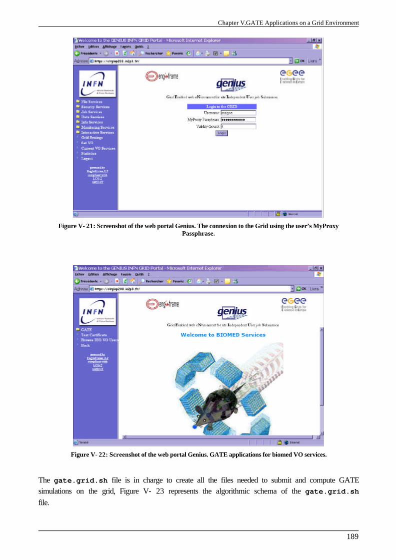
Chapter V.GATE Applications on a Grid Environment
189
Figure V- 21: Screenshot of the web portal Genius. The connexion to the Grid using the user’s MyProxy Passphrase.
Figure V- 22: Screenshot of the web portal Genius. GATE applications for biomed VO services.
The gate.grid.sh file is in charge to create all the files needed to submit and compute GATE simulations on the grid, Figure V- 23 represents the algorithmic schema of the gate.grid.sh file.
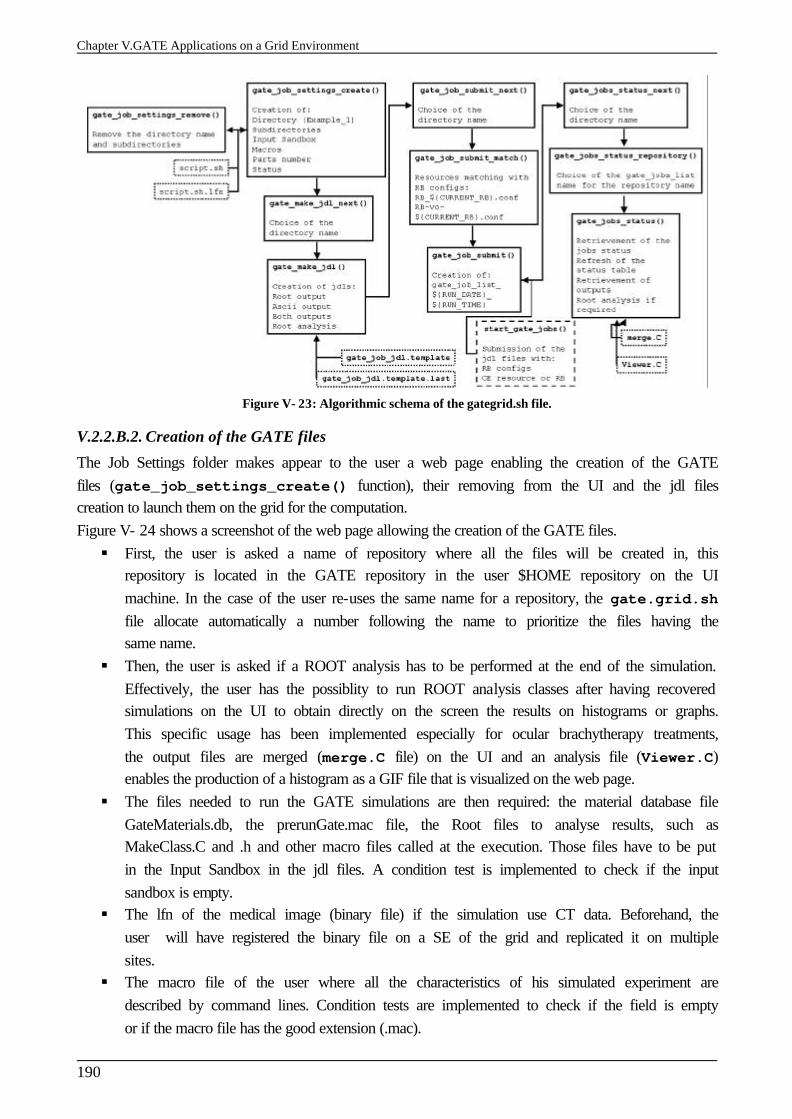
Chapter V.GATE Applications on a Grid Environment
190
Figure V- 23: Algorithmic schema of the gategrid.sh file.
V.2.2.B.2. Creation of the GATE files
The Job Settings folder makes appear to the user a web page enabling the creation of the GATE files (gate_job_settings_create() function), their removing from the UI and the jdl files creation to launch them on the grid for the computation. Figure V- 24 shows a screenshot of the web page allowing the creation of the GATE files. § First, the user is asked a name of repository where all the files will be created in, this
repository is located in the GATE repository in the user $HOME repository on the UI machine. In the case of the user re-uses the same name for a repository, the gate.grid.sh file allocate automatically a number following the name to prioritize the files having the same name.
§ Then, the user is asked if a ROOT analysis has to be performed at the end of the simulation. Effectively, the user has the possiblity to run ROOT analysis classes after having recovered simulations on the UI to obtain directly on the screen the results on histograms or graphs. This specific usage has been implemented especially for ocular brachytherapy treatments, the output files are merged (merge.C file) on the UI and an analysis file (Viewer.C) enables the production of a histogram as a GIF file that is visualized on the web page.
§ The files needed to run the GATE simulations are then required: the material database file GateMaterials.db, the prerunGate.mac file, the Root files to analyse results, such as MakeClass.C and .h and other macro files called at the execution. Those files have to be put in the Input Sandbox in the jdl files. A condition test is implemented to check if the input sandbox is empty.
§ The lfn of the medical image (binary file) if the simulation use CT data. Beforehand, the user will have registered the binary file on a SE of the grid and replicated it on multiple sites.
§ The macro file of the user where all the characteristics of his simulated experiment are described by command lines. Condition tests are implemented to check if the field is empty or if the macro file has the good extension (.mac).

Chapter V.GATE Applications on a Grid Environment
191
§ The number of partitions that corresponds to the splitting number of the simulation. For this splitting especially, the gategrid.sh file is in charge of finding the number of particles emitted in the simulation, the time of emission of those particles and the output file names created in the macro file (for the moment the portal manages ascii and root output formats. In function of the number of partitions, files will be duplicated and the number of particles emitted in each file is divided. A condition test is implemented to check if the number of partitions is between the values 1 and 200.
§ The status files necessary to run simulations by using non overlapping random numbers. A thousand of random status files have been created to launch multiple GATE simulations. Figure V- 25 shows a direct access to the repository STATUS/ in the $HOME/GATE/ repository offered to the user. A condition test is implemented to check if the number of files given by the user is equal to the number of partitions.
§ Finally on the UI, are created the splitted files: the macro files macro###.mac, the script files script###.sh that will be executed on each node, the required files and the status files status###.rndm.
Prepared template files just need to be completed with the requirements of the user automatically by the portal. Figure V- 26 represents the script template that is modified by the GENIUS portal by taking into account the parameters of the user to obtain the final script to be submitted on the grid, see Figure V- 27. The lfn name or Root analysis are taken into account in the script creation if the user selects those fields.
For a number of partitions equal to four, in the GATE repository located in the $HOME, we can see appear the following sub-directories with a Root analysis required: $HOME/GATE/Example_1/macro/
macro000.mac macro001.mac macro002.mac macro003.mac
$HOME/GATE/Example_1/script/ script000.sh script001.sh script002.sh script003.sh
$HOME/GATE/Example_1/required/ GateMaterials.db prerunGate.mac Batch000.C Batch001.C Batch002.C Batch003.C AnalyseClass000.C AnalyseClass001.C AnalyseClass002.C AnalyseClass003.C AnalyseClass000.h AnalyseClass001.h AnalyseClass002.h AnalyseClass003.h
$HOME/GATE/Example_1/status/ status0000.rndm status0001.rndm status0002.rndm
status0003.rndm
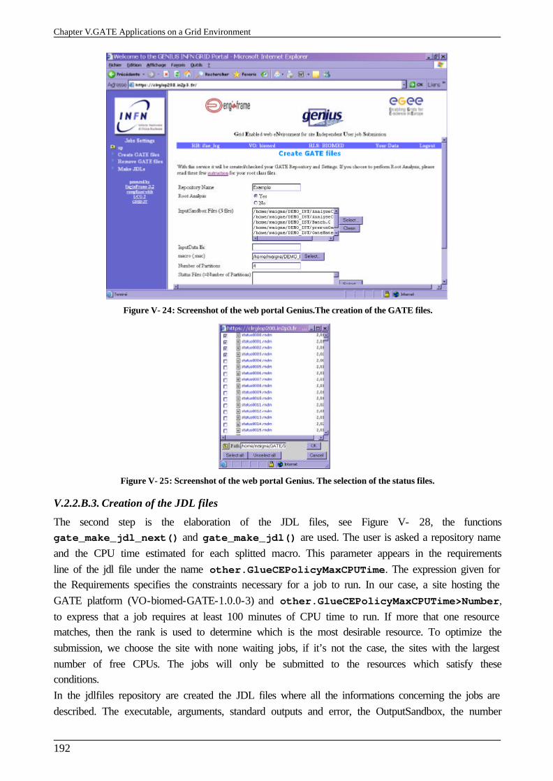
Chapter V.GATE Applications on a Grid Environment
192
Figure V- 24: Screenshot of the web portal Genius.The creation of the GATE files.
Figure V- 25: Screenshot of the web portal Genius. The selection of the status files.
V.2.2.B.3. Creation of the JDL files
The second step is the elaboration of the JDL files, see Figure V- 28, the functions gate_make_jdl_next() and gate_make_jdl() are used. The user is asked a repository name and the CPU time estimated for each splitted macro. This parameter appears in the requirements line of the jdl file under the name other.GlueCEPolicyMaxCPUTime. The expression given for the Requirements specifies the constraints necessary for a job to run. In our case, a site hosting the GATE platform (VO-biomed-GATE-1.0.0-3) and other.GlueCEPolicyMaxCPUTime>Number,
to express that a job requires at least 100 minutes of CPU time to run. If more that one resource matches, then the rank is used to determine which is the most desirable resource. To optimize the submission, we choose the site with none waiting jobs, if it’s not the case, the sites with the largest number of free CPUs. The jobs will only be submitted to the resources which satisfy these conditions. In the jdlfiles repository are created the JDL files where all the informations concerning the jobs are described. The executable, arguments, standard outputs and error, the OutputSandbox, the number
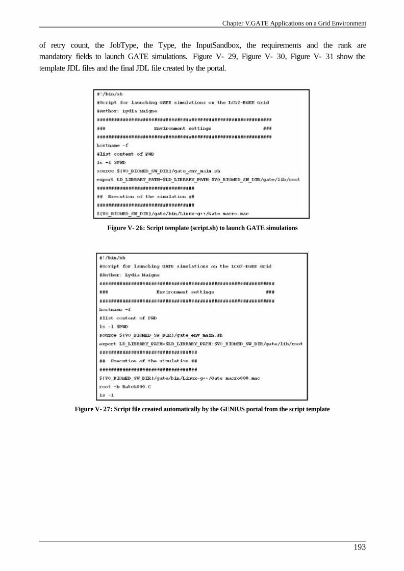
Chapter V.GATE Applications on a Grid Environment
193
of retry count, the JobType, the Type, the InputSandbox, the requirements and the rank are mandatory fields to launch GATE simulations. Figure V- 29, Figure V- 30, Figure V- 31 show the template JDL files and the final JDL file created by the portal.
Figure V- 26: Script template (script.sh) to launch GATE simulations
Figure V- 27: Script file created automatically by the GENIUS portal from the script template
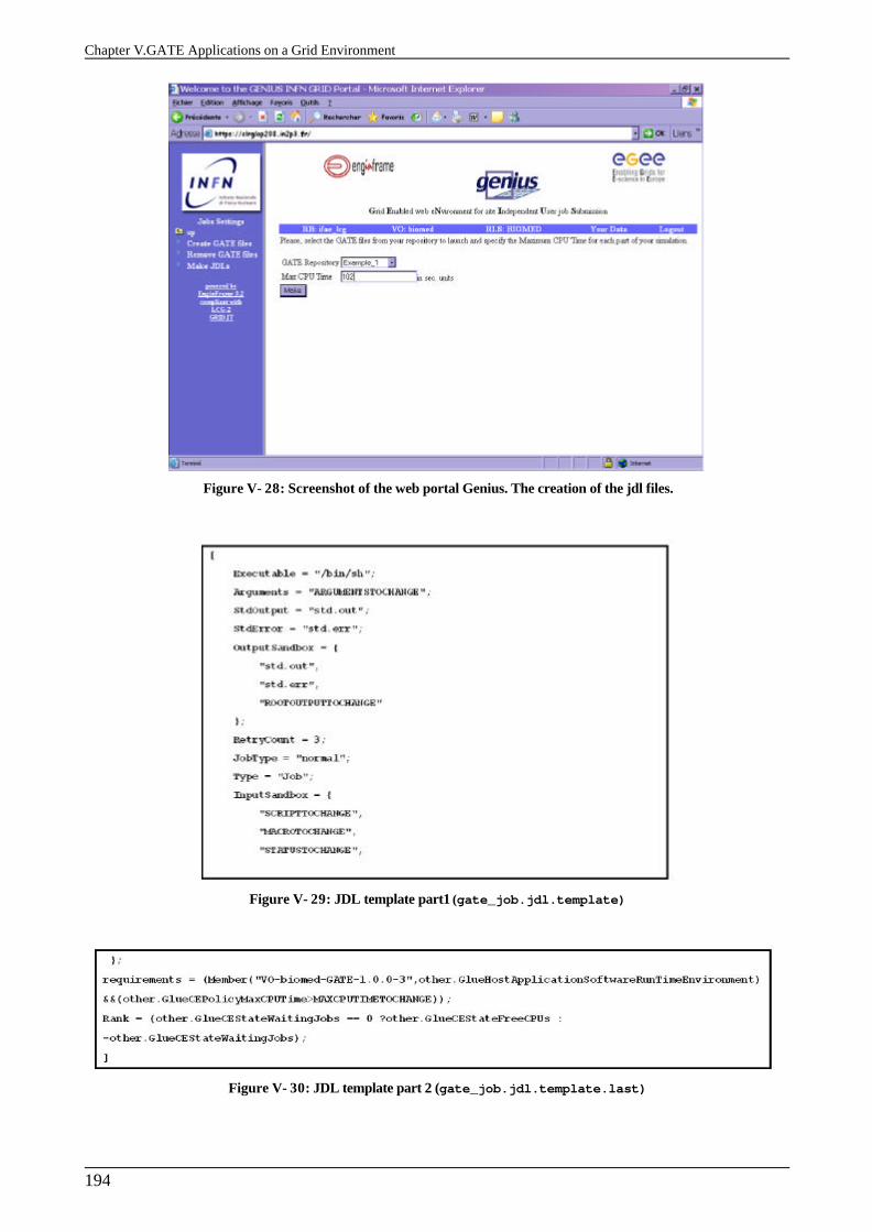
Chapter V.GATE Applications on a Grid Environment
194
Figure V- 28: Screenshot of the web portal Genius. The creation of the jdl files.
Figure V- 29: JDL template part1 (gate_job.jdl.template)
Figure V- 30: JDL template part 2 (gate_job.jdl.template.last)
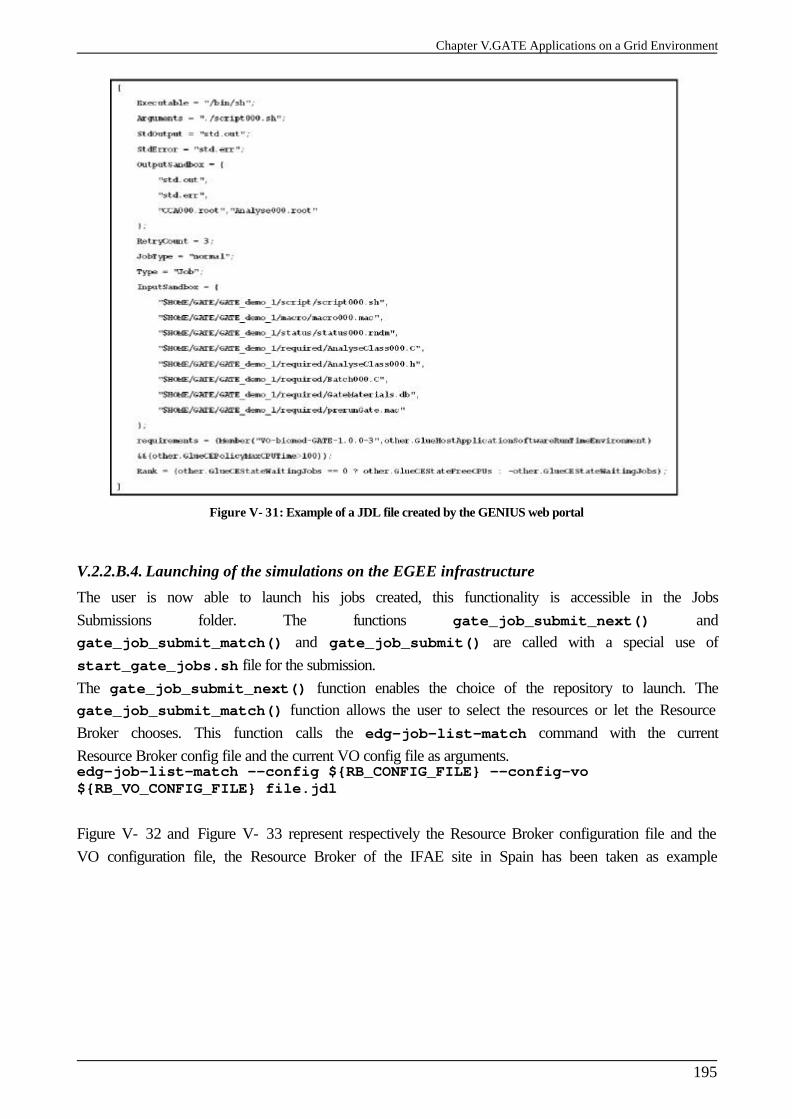
Chapter V.GATE Applications on a Grid Environment
195
Figure V- 31: Example of a JDL file created by the GENIUS web portal
V.2.2.B.4. Launching of the simulations on the EGEE infrastructure
The user is now able to launch his jobs created, this functionality is accessible in the Jobs Submissions folder. The functions gate_job_submit_next() and gate_job_submit_match() and gate_job_submit() are called with a special use of start_gate_jobs.sh file for the submission. The gate_job_submit_next() function enables the choice of the repository to launch. The gate_job_submit_match() function allows the user to select the resources or let the Resource Broker chooses. This function calls the edg-job-list-match command with the current Resource Broker config file and the current VO config file as arguments. edg-job-list-match --config ${RB_CONFIG_FILE} --config-vo ${RB_VO_CONFIG_FILE} file.jdl Figure V- 32 and Figure V- 33 represent respectively the Resource Broker configuration file and the VO configuration file, the Resource Broker of the IFAE site in Spain has been taken as example
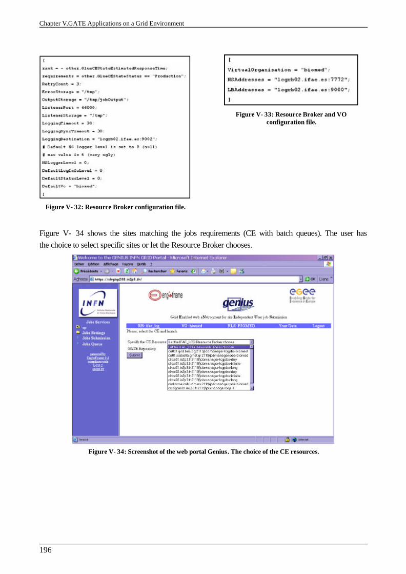
Chapter V.GATE Applications on a Grid Environment
196
Figure V- 32: Resource Broker configuration file.
Figure V- 33: Resource Broker and VO configuration file.
Figure V- 34 shows the sites matching the jobs requirements (CE with batch queues). The user has the choice to select specific sites or let the Resource Broker chooses.
Figure V- 34: Screenshot of the web portal Genius. The choice of the CE resources.
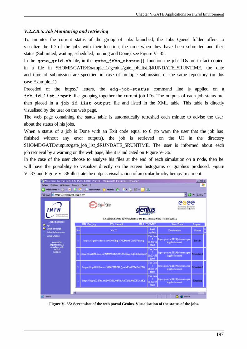
Chapter V.GATE Applications on a Grid Environment
197
V.2.2.B.5. Job Monitoring and retrieving
To monitor the current status of the group of jobs launched, the Jobs Queue folder offers to visualize the ID of the jobs with their location, the time when they have been submitted and their status (Submitted, waiting, scheduled, running and Done), see Figure V- 35. In the gate_grid.sh file, in the gate_jobs_status() function the jobs IDs are in fact copied in a file in $HOME/GATE/Example_1/.genius/gate_job_list_$RUNDATE_$RUNTIME, the date and time of submission are specified in case of multiple submission of the same repository (in this case Example_1). Preceded of the https:// letters, the edg-job-status command line is applied on a job_id_list_input file grouping together the current job IDs. The outputs of each job status are then placed in a job_id_list_output file and listed in the XML table. This table is directly visualised by the user on the web page. The web page containing the status table is automatically refreshed each minute to advise the user about the status of his jobs. When a status of a job is Done with an Exit code equal to 0 (to warn the user that the job has finished without any error outputs), the job is retrieved on the UI in the directory $HOME/GATE/outputs/gate_job_list_$RUNDATE_$RUNTIME. The user is informed about each job retrieval by a warning on the web page, like it is indicated on Figure V- 36. In the case of the user choose to analyse his files at the end of each simulation on a node, then he will have the possibility to visualize directly on the screen histograms or graphics produced. Figure V- 37 and Figure V- 38 illustrate the outputs visualization of an ocular brachytherapy treatment.
Figure V- 35: Screenshot of the web portal Genius. Visualisation of the status of the jobs.
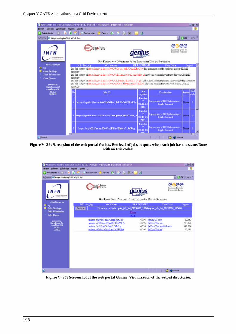
Chapter V.GATE Applications on a Grid Environment
198
Figure V- 36: Screenshot of the web portal Genius. Retrieval of jobs outputs when each job has the status Done with an Exit code 0.
Figure V- 37: Screenshot of the web portal Genius. Visualization of the output directories.
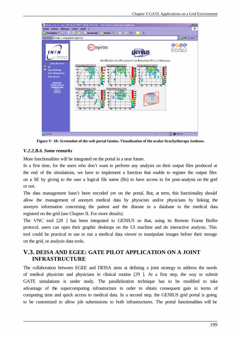
Chapter V.GATE Applications on a Grid Environment
199
Figure V- 38: Screenshot of the web portal Genius. Visualization of the ocular brachytherapy isodoses.
V.2.2.B.6. Some remarks
More functionalities will be integrated on the portal in a near future. In a first time, for the users who don’t want to perform any analysis on their output files produced at the end of the simulations, we have to implement a function that enable to register the output files on a SE by giving to the user a logical file name (lfn) to have access to for post-analysis on the grid or not. The data management hasn’t been encoded yet on the portal. But, at term, this functionality should allow the management of anonym medical data by physicists and/or physicians by linking the anonym information concerning the patient and the disease in a database to the medical data registerd on the grid (see Chapter II. For more details). The VNC tool [28 ] has been integrated to GENIUS so that, using its Remote Frame Buffer protocol, users can open their graphic desktops on the UI machine and do interactive analysis. This tool could be practical to use to run a medical data viewer to manipulate images before their storage on the grid, or analysis data tools.
V.3. DEISA AND EGEE: GATE PILOT APPLICATION ON A JOINT INFRASTRUCTURE
The collaboration between EGEE and DEISA aims at defining a joint strategy to address the needs of medical physicists and physicians in clinical routine [29 ]. At a first step, the way to submit GATE simulations is under study. The parallelization technique has to be modified to take advantage of the supercomputing infrastructure in order to obtain consequent gain in terms of computing time and quick access to medical data. In a second step, the GENIUS grid portal is going to be customized to allow job submissions to both infrastructures. The portal functionalities will be
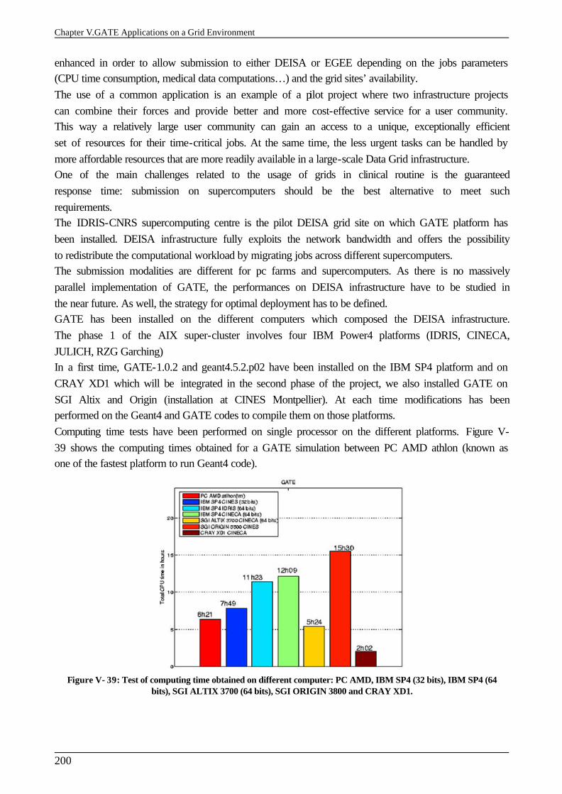
Chapter V.GATE Applications on a Grid Environment
200
enhanced in order to allow submission to either DEISA or EGEE depending on the jobs parameters (CPU time consumption, medical data computations…) and the grid sites’ availability. The use of a common application is an example of a pilot project where two infrastructure projects can combine their forces and provide better and more cost-effective service for a user community. This way a relatively large user community can gain an access to a unique, exceptionally efficient set of resources for their time-critical jobs. At the same time, the less urgent tasks can be handled by more affordable resources that are more readily available in a large-scale Data Grid infrastructure. One of the main challenges related to the usage of grids in clinical routine is the guaranteed response time: submission on supercomputers should be the best alternative to meet such requirements. The IDRIS-CNRS supercomputing centre is the pilot DEISA grid site on which GATE platform has been installed. DEISA infrastructure fully exploits the network bandwidth and offers the possibility to redistribute the computational workload by migrating jobs across different supercomputers. The submission modalities are different for pc farms and supercomputers. As there is no massively parallel implementation of GATE, the performances on DEISA infrastructure have to be studied in the near future. As well, the strategy for optimal deployment has to be defined. GATE has been installed on the different computers which composed the DEISA infrastructure. The phase 1 of the AIX super-cluster involves four IBM Power4 platforms (IDRIS, CINECA, JULICH, RZG Garching) In a first time, GATE-1.0.2 and geant4.5.2.p02 have been installed on the IBM SP4 platform and on CRAY XD1 which will be integrated in the second phase of the project, we also installed GATE on SGI Altix and Origin (installation at CINES Montpellier). At each time modifications has been performed on the Geant4 and GATE codes to compile them on those platforms. Computing time tests have been performed on single processor on the different platforms. Figure V- 39 shows the computing times obtained for a GATE simulation between PC AMD athlon (known as one of the fastest platform to run Geant4 code).
Figure V- 39: Test of computing time obtained on different computer: PC AMD, IBM SP4 (32 bits), IBM SP4 (64 bits), SGI ALTIX 3700 (64 bits), SGI ORIGIN 3800 and CRAY XD1.
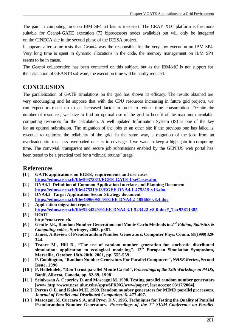
Chapter V.GATE Applications on a Grid Environment
201
The gain in computing time on IBM SP4 64 bits is inexistent. The CRAY XD1 platform is the more suitable for Geant4-GATE execution (72 biprocessors nodes available) but will only be integered on the CINECA site in the second phase of the DEISA project. It appears after some tests that Geant4 was the responsible for the very low execution on IBM SP4. Very long time is spent in dynamic allocations in the code, the memory management on IBM SP4 seems to be in cause. The Geant4 collaboration has been contacted on this subject, but as the IBM/xlC is not support for the installation of GEANT4 software, the execution time will be hardly reduced. CONCLUSION The parallelization of GATE simulations on the grid has shown its efficacy. The results obtained are very encouraging and let suppose that with the CPU resources increasing in future grid projects, we can expect to reach up to an increased factor in order to reduce time consumption. Despite the number of resources, we have to find an optimal use of the grid to benefit of the maximum available computing resources for the calculation. A well updated Information System (IS) is one of the key for an optimal submission. The migration of the jobs to an other site if the previous one has failed is essential to optimize the reliability of the grid. In the same way, a migration of the jobs from an overloaded site to a less overloaded one is to envisage if we want to keep a high gain in computing time. The convivial, transparent and secure job submissions enabled by the GENIUS web portal has been tested to be a practical tool for a “clinical routine” usage. References [1 ] GATE applications on EGEE, requirements and use cases
https://edms.cern.ch/file/503738/1/EGEE-GATE-UseCases.doc [2 ] DNA4.1 Definition of Common Application Interface and Planning Document
https://edms.cern.ch/file/475319/13/EGEE-DNA4.1-475319-v13.doc [3 ] DNA4.2 Target Application Sector Strategy document
https://edms.cern.ch/file/489669/8.4/EGEE-DNA4.2-489669-v8.4.doc [4 ] Application migration report
https://edms.cern.ch/file/523422//EGEE-DNA4.3.1-523422-v8-0.doc#_Toc93811385 [5 ] ROOT
http://root.cern.ch/ [6 ] Gentle J.E., Random Number Generation and Monte Carlo Methods in 2nd Edition, Statistics &
Computing collec, Springer, 2003, p381. [7 ] James, A Review of Pseudorandom Number Generators, Computer Phys. Comm. 60 (1990) 329-
344. [8 ] Traore M., Hill D., “The use of random number generation for stochastic distributed
simulation: application to ecological modeling”. 13th European Simulation Symposium, Marseille, October 18th-20th, 2001, pp. 555-559
[9 ] P. Coddington, "Random Number Generators For Parallel Computers", NHSE Review, Second Issue, 1996
[10 ] P. Hellekalek, "Don’t trust parallel Monte Carlo!", Proceedings of the 12th Workshop on PADS, Banff, Alberta, Canada, pp. 82-89, 1998
[11 ] Srinivasan A. Ceperley D. and Mascagni M. 1998. Testing parallel random number generators [www http://www.ncsa.uiuc.edu/Apps/SPRNG/www/paper/, last access: 03/17/2004].
[12 ] Percus O.E. and Kalos M.H. 1989. Random number generators for MIMD parallel processors. Journal of Parallel and Distributed Computing. 6. 477-497.
[13 ] Mascagni. M. Cuccaro S.A. and Pryor D.V. 1995. Techniques for Testing the Quality of Parallel Pseudorandom Number Generators. Proceedings of the 7th SIAM Conference on Parallel Processing for Scientific Computing. 279-284.
Chapter V.GATE Applications on a Grid Environment
202
Processing for Scientific Computing. 279-284. [14 ] Srinivasan A. 1998. Introduction to Parallel RNG [www http://archive.ncsa.uiuc.edu/
Science/CMP/RNG/www/paper/index.html, last access: 03/17/2004]. [15 ] G. Marsaglia and A. Zaman, Toward a Universal Random Number Generator, Florida State
University FSU-SCRI-87-50 (1987). [16 ] CLHEP Reference Guide
(http://wwwinfo.cern.ch/asd/lhc++/clhep/manual/RefGuide/index.html) [17 ] Noell Karl-L, Weber H. Faxhhochschule Wiesbaden, W. Germany, Department of Computer
Science. http://astronomy.swin.edu.au/~pbourke/analysis/random/randomlib.c
[18 ] CLHEP User Manual (http://wwwinfo.cern.ch/asd/lhc++/clhep/manual/UserGuide/index.html). (http://wwwinfo.cern.ch/asd/geant/geant4_public/Random.html).
[19 ] Segal B., “Grid computing : the European data project”, IEEE Nuclear Science Symposium and Medical Imaging Conference, Lyon, 15-20 October 2000.
[20 ] P. Calvat, JJS tool http://cc.in2p3.fr in Accueil>Espace Utilisateurs > Service et outils > Téléchargements
[21 ] R-GMA: Production Services for Information and Monitoring in the Grid Paper presented by John Walk at AHM2004 in Nottingham, UK http://hepunx.rl.ac.uk/egee/jra1-uk/
[22 ] C.O. Thiam, D. Donnarieix, V. Breton, Z. El Bitar, L. Maigne, « Computing grids for medical physics », proceedings of the 44èmes journées de la SFPM, Avignon 2005.
[23 ] INFN Grid Project http://grid.infn.it/
[24 ] NICE srl, EngineFrame http://engineframe.com
[25 ] ‘GENIUS: a web portal for the grid’,G.Andronico,R.Barbera,A.Falzone,G.Lo Re,A. Pulvirenti, A.Rodolico, Nucl.Instr.Meth. in Phys. Res. A 502 (2003) 433
[26 ] ‘GENIUS:a simple way to access computational and data grids’,G.Andronico,R.Barbera,A.Falzone,G.LoRe,A.Pulvirenti,A.Rodolico,Future Generation of Computer Systems 19 (2003) 805.
[27 ] GENIUS web site https://genius.ct.infn.it
[28 ] GILDA: the Grid INFN virtual Laboratory for Dissemination Activities’, G.Andronico, V. Ardizzone, R.Barbera, R.Catania,A.Carrieri,A.Falzone, E.Giorgio, G.La Rocca,S.Monforte, M.Pappalardo, G.Passaro, G.Platania, Proceedings of Tridentcom 2005, in press on IEEE Computer.
[29 ] TightVNC http://www.tightvnc.com/
[30 ] European Grid Project Synergy Roadmap in collaboration with DEISA and SEE-GRID EGEE DNA5.2 https://edms.cern.ch/document/533194
General Conclusion
203
General Conclusion This thesis aimed at the creation of a convivial usage of Monte Carlo simulations in clinical practice for dosimetry applications. The study of these features implied the validation of the GATE platform using the GEANT physics libraries for absorbed dose calculations concerning electrons, particularly in ocular brachytherapy. It has been decided to exploit a grid architecture functionalities to distribute our accurate Monte Carlo simulations in order to obtain a significant gain in computation time to compete with analytic softwares currently used in hospitals for radiotherapy treatment plannings. Since 2002, the GATE platform has been used for dosimetry applications in PCSV team. This work has been encouraged by the creation of two working groups among the OpenGATE collaboration after the release of the open source GATE package in May 2004: one concerning dosimetry and an other for cluster/grid processing. In addition, the involvement of our team and the Laboratoire de Physique Corpusculaire in the DataGrid and next in the EGEE projects enabled us to propose innovative solutions to reduce the computation time of our Monte Carlo platform in order to use it in a clinical practice or help researchers in their work. GATE and a grid infrastructure were the two primary tools to enable the approach of fast and accurate dosimetry calculations for a clinical practice. GATE has been first designed to answer the needs in SPECT and PET applications, the idea was to deal with this platform for dosimetric studies in brachytherapy and radiotherapy applications. As it has been demonstrated, the primary functionalities of the platform are not yet sufficient for a convivial and dedicated usage of Monte Carlo code for dosimetric studies but are encouraging. The first aspect is that geometry encoding is still restricted to simple predefined volumes that can’t be associated or can’t be overlaped between each other which limits the creation of complex geometries. Then, there’s no dedicated system for linear accelerators or radioactive sources features. Output data of the simulations concern for the moment basic information concerning each interaction of particles in media such like energy deposited and the position of interactions in space. A necessary implementation is required to evaluate the dose deposited in volumes of interest directly from the simulation without a post-analysis of data. Despite those negative points, the GATE platform with its ease of use, proposes or will propose in a near future attractive and convenient tools for dosimetry. The major asset of the platform is the possibility to import CT images in the simulations to describe patient’s body. The encoding of
General Conclusion
204
parameterised volumes in the platform will improve the tracking of particles in voxelized matrices representing tissue heterogeneities. The visualization of such matrices will also benefit of this feature. Validation of physic processes encoded in GEANT4 implying electrons is also a necessary step to compete with other Monte Carlo codes such as EGSnrc for which electron transport has been better developed with improved energy loss evaluation techniques and correct fictitious discret interactions. The simulation of monoenergetic and polyenergetic electron dose point kernels using GEANT4 standard and lowenergy physics packages and the comparison with other Monte Carlo codes of interest in the field of dosimetric applications has shown discrepancies. Differences between GEANT4 versions (5.2.p02, 6.2.p02 and 7.0.p01) in the simulation of the kernels highlighted the fact that the multiple scattering implementation was in cause with an inadequate angular distribution definition. A new implementation of the process is due in the release 8.0 of the GEANT4 software. In a second step, GATE using the standard package of GEANT4 version 6.2.p02 was tested for ocular brachytherapy treatment simulations using 106Ru/106Rh beta emitter sources. Comparisons of GATE results with other Monte Carlo, measurements and analytic calculations provided by the treatment planning software used in clinical practice showed a good behaviour of the platform for such dosimetry. In order to use CT data in GATE simulations, a procedure enabling the correlation between CT numbers and tissue parameters (density and atomic weights) has been developed and tested. This study has shown a well determination of the calcium, phosphorus and hydrogen weights in skeletal tissues. Carbon and oxygen weights in tissues (in particularly soft tissues) are poorly resolved by means of the CT numbers which imply to find an other alternative to describe soft tissues, for example using MRI images. Results of GATE calculations show the impact of atomic weights definition on dose distributions from electron and photon beams. As the computation time is one the major limiting factor for the utilization of Monte Carlo in a clinical practice, we engaged into splitting the simulations in a grid environment by taking into account the non reproducibility of the calculations. To achieve this goal, a detailed analysis of the Random Number Generator used by the GATE platform was done with an evaluation of the consumption in random numbers for different simulations in medical physic fields. As a consequence, a thousand of independent random number sequences were produced with a suitable size in order to fit the duration of simulations. We tested how the functionalities offered by a grid infrastructure could answer the needs in reducing the computation time and also could fit the requirements imposed by a deployment of tools for the medical staff. The DataGrid project was the first grid infrastructure on which we tested the parallelization of GATE simulations using the independent sequence splitting of the random number generator. Results concerning computation challenges obtained during the second year of the project was very encouraging. We reached up to a speed-up factor of 7.78 by splitting in 20 simulations, a simulation running in more than 2 hours and 30 minutes on a single 1.5 GHz processor. The deployment of GATE simulations on the EGEE production grid infrastructure
General Conclusion
205
improved again the gain in computation time thanks to the federation of more computing resources. An important speed-up factor of 28.2 was reached during our tests. An other major development integrated in this thesis was the creation of web services allowing the transparent submission of GATE simulations in a grid environment. The GATE platform was first packaged and installed on the 20 nodes of the grid hosting the biomed organisation at this date. An efficient and fast procedure of installation on the grid using grid middleware functionalities has been set up. Because of its multi-layered security infrastructure, the web portal GENIUS was chosen to host the encoding modalities to launch in a transparent way GATE simulations on the EGEE infrastructure. The functionalities encoded allow the end user to enter its GATE simulation and files associated to in order that it is divided into smaller simulations by associating independent random number sequences. The preparation of the necessary files to launch jobs on the grid are automatically created in background. The functionalities enable also the allocation of medical images to the simulations in the case of calculations on CT patient data for which GATE is able to plan a dosimetry. A first prototype of the GENIUS web portal (https://clrglop208.in2p3.fr) hosting GATE functionalities is now available using a secure internet connection and grid certificates. The web portal is accessible from the Centre Jean Perrin where medical physicists are able to launch GATE simulations on ocular brachytherapy using 106Ru/106Rh applicators. We can’t conclude at this date that GATE simulations distributed on a grid environment are used for clinical routine treatment planning. To enable such usage in a near future the work performed in this PhD thesis has to be followed by additional studies. Concerning the usage and testing of grid added value in the reduction of the calculation time for GATE simulations, some points have to be detailed following this priority order: § Large scale grid computing time tests need to be performed to evaluate failures and the gain
in time occuring in a daily usage of the grid. § Alternatives have to be proposed against grid bottlenecks that prevent a usage of the GATE
simulations in clinical practice, for example: the Resource Broker failures and the computing resources load balancing.
§ Encoding of the management of medical images in the next releases of the GENIUS web portal should be studied. Associated to a relational database located at hospital, it would enable the correlation between metadata related to patient such as the name, the pratician, the characteristics of the disease, etc, and anonym medical images registered on the grid.
§ A simplified utilization of the GENIUS web portal should be developed to allow its use by novice users. No time should be spent by the medical physicist or pratician to assimilate the functionalities proposed by the web portal, its utilization should be as intuitive as required. For the moment the prototype version has required training course to use it.
General Conclusion
206
Concerning the validation of the GATE platform for dosimetry applications: § dedicated developments for dosimetric applications in GATE, with the creation of new
systems to define linear accelerators and radioactive sources. Output data concerning dose deposited should also be implemented to facilitate the usage of the platform.
§ A validation of the GEANT4 accuracy for dosimetric calculations implying electrons. The criteria of comparison of the GATE platform with other Monte Carlo codes for dosimetry should take into account the availability, convenience of use, flexibility for simulating complex detector geometries and experimental arrangements and support and maintenance. In that way, GATE should be compared with the GEANT release 8.0 in a near future especially with EGSnrc and MCNP.
§ a validation of the incorporation of CT data in GATE simulations by benefiting of the transcription of CT numbers into tissue parameters developed in this thesis. This work would deserve a validation and a comparison with results obtained in homogeneous medium to estimate better the influence of density and atomic composition of tissue on dose distributions. Ocular brachytherapy treatments would benefit of an accurate location of the tumour with an allocation of correct density and tissue parameters to uveal melanoma and some eye structures.
Conclusion générale
207
Conclusion générale Cette thèse a abouti à la création d’une utilisation conviviale des simulations Monte Carlo en routine clinique pour les applications en dosimétrie. Cette étude a impliqué la validation de la plate-forme GATE utilisant les librairies physiques de GEANT4 pour le calcul de la dose absorbée par des électrons, notamment pour la curiethérapie oculaire. Il a été décidé d’exploiter les fonctionnalités d’une architecture de grille pour distribuer nos simulations Monte Carlo afin d’obtenir un gain significatif en temps de calcul de manière à rivaliser avec les logiciel analytiques actuellement utilisés en centres hospitaliers pour les planifications de traitement en radiothérapie. Depuis 2002, la plate-forme de simulation GATE a été utilisée pour des applications en dosimétrie dans l’équipe PCSV. Ce travail a été encouragé par la création de deux groupes de travail au sein de la collaboration OpenGATE après la parution du premier package dont les fichiers sources ont été rendus disponibles en mai 2004 : un concernant les calculs en dosimétrie et le second concernant le calcul sur ferme ou grille. De plus, la participation de notre équipe et du Laboratoire de Physique Corpusculaire dans les projets DataGrid et par la suite EGEE nous ont permis de proposer des solutions innovantes pour réduire le temps de calcul de notre plate-forme Monte Carlo dans le but de l’utiliser en routine clinique ou d’aider des chercheurs dans leur travail. GATE et l’infrastructure de grille ont été les deux outils premiers permettant une approche rapide et précise des calculs de dosimétrie pour la routine clinique. GATE a été dans un premier temps élaboré pour répondre aux besoins en imagerie SPECT et TEP, mais l’idée était d’utiliser cette plate-forme également pour des études dosimétriques en curiethérapie et radiothérapie. Comme il a été démontré, les premières fonctionnalités de la plate-forme ne sont pas encore suffisantes pour une utilisation conviviale et dédiée aux études dosimétriques mais sont néanmoins encourageantes. L’encodage des géométries dans GATE est restreint à l’utilisation de volumes géométriques simples prédéfinis qui ne peuvent ni être associées ni se recoupés pour créer des volumes complexes. De plus, aucun système n’est dédié pour la modélisation d’accélérateurs linéaires ou de sources radioactives. Enfin, les sorties de données des simulations traitent des informations standard relatives aux interactions des particules dans un milieu comme l’énergie déposée ou les positions d’interactions dans l’espace. Une implémentation est nécessaire pour permettre le calcul de dose déposée dans des volumes d’intérêt directement à l’issue d’une simulation et non plus grâce à une post-analyse des données.
Conclusion générale
208
En dépit de ces points négatifs, la plate-forme GATE avec sa facilité d’utilisation propose ou proposera dans un futur proche des outils pratiques et interactifs pour la dosimétrie. L’atout majeur de la plate-forme est la possibilité d’importer des images scanner dans les simulations pour décrire le corps du patient. L’encodage des volumes paramétrés dans GATE permettra le suivi des particules dans des matrices de voxels représentant les hétérogénéités des tissus. La visualisation aisée de ces matrices bénéficiera aussi de cette caractéristique. La validation des processus physiques encodés dans GEANT4 et impliquant les électrons est une étape nécessaire pour rivaliser avec d’autres codes Monte Carlo, en particulier EGSnrc pour lequel le transport des électrons a été développé avec une meilleure évaluation des techniques de perte d’énergie et des interactions discrètes corrigées. La simulation de point kernel d’électrons mono-énergétiques et poly-énergétiques utilisant les packages standard et basse énergie de GEANT4 ainsi que la comparaison avec d’autres codes Monte Carlo d’intérêt dans le domaine des applications dosimétriques ont montré des différences. Les différences entre les versions de GEANT4 (5.2.p02, 6.2.p02 et 7.0.p01) dans la simulation des points kernels a mis en évidence le fait que l’implémentation de la diffusion multiple était en cause avec une définition inappropriée de la distribution angulaire. Une nouvelle implémentation de ce processus est prévue pour la version 8.0 du logiciel GEANT4. Dans un deuxième temps, GATE utilisant le package standard de la version 6.2.p02 de GEANT4 a été testé pour des simulations de traitement de curiethérapie oculaire utilisant des sources de 106Ru/106Rh émettrices béta. Les comparaisons des résultats obtenus avec GATE et d’autres calculs Monte Carlo ainsi que des mesures et des calculs analytiques fournis par le logiciel de planification de traitement utilisé en routine clinique, ont montré un bon comportement de la plate-forme pour ce type de dosimétrie. Dans le but d’utiliser des données scanner dans les simulations GATE, une procédure a été développée et testée pour permettre une corrélation entre les nombres Hounsfield et les paramètres tissulaires (densité et poids atomiques). Cette étude a montré une bonne détermination des composés calcium, phosphore et hydrogène dans les tissus osseux. Les composés carbone et oxygène dans les tissus (en particulier les tissus mous) sont mal quantifiés au moyen des nombres Hounsfield ce qui implique de trouver une autre alternative pour décrire les tissus mous, par exemple en s’aidant des données de l’IRM. Les simulations GATE réalisées montrent l’impact de la définition des composés atomiques sur les distributions de dose causées par des faisceaux de photons et d’électrons. Comme le temps de calcul est un des facteurs majeurs limitant l’utilisation du Monte Carlo en pratique clinique, nous nous sommes engagés à diviser les simulations dans un environnement de grille en prenant en compte la non reproductibilité des calculs. Pour atteindre ce but, une analyse détaillée du générateur de nombres aléatoires utilisé par la plate-forme GATE a été effectuée avec une évaluation de la consommation de nombres aléatoires pour différentes simulations dans les domaines de la physique médicale. En conséquence, mille séquences de nombres pseudo-aléatoires de taille suffisante pour correspondre avec la durée des simulations réalisées, ont été produites.
Conclusion générale
209
Nous avons testé comment les fonctionnalités offertes par la grille pouvaient répondre aux besoins de réduction du temps de calcul et aussi au déploiement d’outils pour une équipe de soin médicale. Le projet DataGrid a mis en place la première infrastructure de grille sur laquelle nous avons testé la parallélisation des simulations GATE en utilisant des séquences indépendantes du générateur de nombres aléatoires. Les résultats concernant les challenges impliqués par de tels calculs ont été encourageants durant la deuxième année du projet. Un gain de 7.78 a été atteint en divisant une simulation se déroulant en plus de 2h30 sur un simple processeur de 1.5GHz en 20 simulations. Le déploiement des simulations GATE sur l’infrastructure de grille de production EGEE a amélioré encore ce gain grâce à la fédération de plus importantes ressources de calcul. Un gain maximum de 28.2 a été atteint durant nos tests. Un autre développement majeur intégré dans ce travail de thèse a été la création de services web permettant la soumission transparente de simulations GATE sur un environnement de grille. La plate-forme GATE a été tout d’abord packagée et installée sur 20 nœuds de la grille accueillant l’organisation biomed à ce jour. Une procédure d’installation rapide et efficace utilisant les fonctionnalités de l’intergiciel de grille a été mis en place. Grâce à son infrastructure de sécurité « multi-couches », le portail web GENIUS a été choisi pour accueillir les modalités pour soumettre de manière transparente, les simulations GATE sur l’infrastructure EGEE. Les fonctionnalités encodées permettent à l’utilisateur final de diviser sa simulation ainsi que ses fichiers associés en de plus petites simulations en associant à chacune d’elle une séquence de nombres aléatoires indépendante. La préparation des fichiers nécessaires pour le lancement des jobs sur la grille sont automatiquement crées en arrière plan. Les fonctionnalités permettant une allocation d’images médicales aux simulations dans le cas d’une planification de traitement utilisant des images scanner avec GATE sont disponibles. Un premier prototype du portail GENIUS accueillant les fonctionnalités pour GATE (https://clrglop208.in2p3.fr) est à présent disponible en utilisant une connexion internet sécurisée et des certificats d’authentification pour l’accès à l’infrastructure de grille. Le portail web est accessible depuis le Centre Jean Perrin où des physiciens médicaux sont capables de lancer des simulations GATE pour des traitements de curiethérapie oculaire utilisant des applicateurs de 106Ru/106Rh. Nous ne pouvons pas conclure à ce jour que les simulations GATE sont utilisées pour la planification des traitement en routine clinique grâce à l’environnement de grille de calcul. De manière à permettre une telle issue, le travail commencé au cours de cette thèse doit être poursuivi par des études additionnelles. Concernant l’étude des performances de la valeur ajoutée de la grille sur la réduction des temps de calcul des simulations, d’autres points sont à étudiés suivant cet ordre de priorité : § Des tests de temps de calcul à plus grande échelle sont nécessaires pour évaluer les limites
ainsi que le gain pouvant être obtenus par une utilisation journalière de la grille.
Conclusion générale
210
§ Des alternatives doivent être trouvées contre les goulots d’étranglements inhérent à la grille pour une utilisation de GATE en routine clinique, nous pouvons citer à titre d’exemple les inconvénients du Resource Broker et la distribution de la charge sur les ressources de calcul.
§ Les fonctionnalités concernant la gestion des images médicales sur grille devraient être encodées au niveau du portail web GENIUS. Associées à une base de données relationnelles localisée en centre hospitalier, la corrélation entre les méta-données relatives au patient, comme le nom du patient, du praticien, les caractéristiques de la maladie, etc, et les images médicales anonymes enregistrées sur la grille.
§ Une utilisation plus simplifiée du portail GENIUS devrait être mise en place pour les utilisateurs novices. Il est à prohiber une utilisation du portail qui ne serait pas la plus intuitive possible. Jusqu’à présent, l’utilisation du portail web a nécessité de cours pour apprendre son fonctionnement.
Concernant la validation de la plate-forme GATE pour les applications en dosimétrie : § Des développements dédiés pour effectuer des études dosimétriques avec GATE sont
nécessaires, de nouveaux systèmes aidant à la modélisation d’accélérateurs linéaires et de sources radioactives scellées sont à pourvoir. Les sorties de données relatives aux dose déposées devraient être implémentées.
§ Une validation du logiciel GEANT4 pour les applications en dosimétrie utilisant les électrons doit être poursuivie. De plus, les critères de choix de la plate-forme GATE en comparaison d’autres Monte Carlo devront se baser sur son accessibilité, sa facilité d’utilisation, sa flexibilité à simuler des géométries de détecteur complexes, des procédés de mesures expérimentales ainsi qu’un support et une maintenance du code. Dans cette perspective, GATE associé à la version 8.0 de GEANT4 devrait être comparé avec EGSnrc et MCNP.
§ Une validation concernant l’incorporation d’images scanner dans les simulations GATE doit être faite en bénéficiant de la transcription des nombres Hounsfield en paramètres tissulaires effectuée au cours de cette thèse. Ce travail servirait de validation et de comparaison avec des résultats obtenus en milieu homogène pour mieux estimer l’influence de la densité et de la composition atomique des tissus sur les distributions de dose. Les traitements de curiethérapie oculaire bénéficieraient en outre d’une meilleur localisation de la tumeur avec une allocation correcte de la densité et des paramètres tissulaires des mélanomes de l’uvée et des structures oculaires.
Figures and Tables
211
Figures and Tables Figures Figure I- 1: Simplified schema of the eye anatomy 12 Figure I- 2: Fundus of patient’s eye 14 Figure I- 3: Fundus image of a choroidal melanoma 14 Figure I- 4: Ocular echography of a patient 14 Figure I- 5: Echography image of an ocular melanoma 14 Figure I- 6: Frontal view of a patient eye obtain with MRI (choroidal melanoma) 15 Figure I- 7: Sagittal view of a patient eye obtained with MRI (choroidal melanoma) 15 Figure I- 8: Decay scheme of 106Ru/106Rh nuclide 16 Figure I- 9: Beta spectrum of 106Rh 16 Figure I- 10: Scheme of an ophthalmic applicator 17 Figure I- 11: Photos of some 106Ru/106Rh ophthalmic applicators 17 Figure I- 12: 16 types of Ru-106 ophthalmic plaques. The radioactive area is marked hatched. 18 Figure I- 13: COMS iodine-125 ophthalmic applicators 20 Figure I- 14: Iodine-125 seeds in a COMS ophthalmic applicator. 20 Figure I- 15: Encapsulation of the iodine-125 seeds in a COMS applicator 20 Figure I- 16: Ocular nozzle and proton beam line schema of the Nice hadrontherapy platform. 22 Figure I- 17: The ocular nozzle 22 Figure I- 18: NIST WT1 solid phantoms used for depth dose measurements. 29 Figure I- 19: NIST WT1 solid phantom with different cap heights used for the concave ophthalmic applicators. 29 Figure I- 20: RMI457 solid water phantom and GAFCHROMIC MD-55 film, 29 Figure I- 21: Eye contours, position and size determination on a CT image with Plaque Simulator. 34 Figure I- 22: Patches inside an ophthalmic applicator. 35 Figure I- 23: The angle f used to calculate F(r,f) is defined as the angle between a vector n originating at the effectivecenter c of a patch and directed towards the center of the sphere to which the applicator conforms, and a vector from c to the dose calculation point p. r is the distance between c and p. 35 Figure I- 24: Plotted equations of the geometry factor G(r) over the range 0 to 8mm. The solid line is the inverse square function (Equation I- 12) and the dashed line is the linear function (Equation I- 13) for the model CCB applicator with crossover distance xn=1.65 mm and slope m=2. 36 Figure I- 25: Central axis measurements entered in the Plaque Simulator treatment planning system. 37 Figure I- 26: Surface measurements entered in the Plaque Simulator treatment planning system. 37
Figures and Tables
212
Figure I- 27: Prescription window. The date of the plaque insertion and the date of the plaque removal are fixed to obtain 500 Gy at 1 mm in depth on the central axis using a CCA applicator. 38 Figure I- 28: Isodoses obtained with Plaque Simulator with a CCA applicator. 38 Figure II- 1: Evolution of the EGEE middleware 56 Figure II- 2: gLite services 56 Figure II- 3: Job flow in EGEE 61 Figure II- 4: DM2 interface between medical imagers and the grid 70 Figure III- 1: Network image transfer with the DICOM standard 78 Figure III- 2: Image Information Object Definition 79 Figure III- 3: Real data flow that can be read in a DICOM file 81 Figure III- 4: Interfile 3.3 key-value pairs describing a binary image data. 82 Figure III- 5: Bytes encoding for Little and Big Endian modalities. 83 Figure III- 6: Allocation and storage of data in pixels in DICOM3 standard 84 Figure III- 7:File range.dat defining the transcription of binary number ranges into materials. 85 Figure III- 8: Schema of the classes implied in the creation of a ReplicaMatrix 86 Figure III- 9:Schema of the classes implied in the visualisation of the ReplicaMatrix 86 Figure III- 10: Principle of geometrical importance sampling: the cells on the left have half importance the cells on the right. Figure (a): the track is splitted in two tracks with half the weight. Figure (b): The track is either deleted or its weight is doubled after surviving Russian Roulette. 88 Figure III- 11: Simple importance map configuration for a water phantom and a single SPECT detector head. 89 Figure III- 12: Visualization of the collision of a photon with the collimator and the backscatter particles created. 90 Figure III- 13: Simple particle history with branching: “v” indicates a geometrical importance split while “p” indicates a physical split. All tracks are numbered according the numbering rules in GEANT4 90 Figure III- 14: Two physically possible branches from the right side of Figure III- 12. 91 Figure III- 15: Three physically possible branches from the left side of Figure III- 12. 91 Figure III- 16: File “info.visu” describing the medical data: name of the image,transcription file, number of voxels and their dimensions 92 Figure III- 17: Screenshot of the C++ module enabling the visualisation of medical data. On the left part, the dialogue screen enable the user to manage the image. On the right part the creen of visualisation 93 Figure III- 18: Range of materials between 19 and 80 H visualized in red color by the Linux viewer. 93 Figure III- 19: Range definition 97 Figure III- 20: ESTAR: Stopping Powers and Range Tables for Electrons 97 Figure III- 21: Goodness-of-Fit test results concerning the electron stopping power plotted as a function of the atomic number Z of the selected elements (Standard: black diamonds, Low Energy EPDL: black squares, Low Energy Penelope approach: empty circles). All the p-values obtained are higher than the confidence level set (a = 0.05). 105 Figure III- 22: Comparison of GATE_G4 versions calculated dose point kernels for 50 keV electrons with EGSnrc (Mainegra), EGS4 (Simpkin and Mackie), ACCEPT (Cross) and MCNP4c. 108 Figure III- 23: Comparison of GATE_G4 versions calculated dose point kernels for 100 keV electrons with EGSnrc (Mainegra), EGS4 (Simpkin and Mackie), ACCEPT (Cross) and MCNP4c. 109 Figure III- 24: Comparison of GATE_G4 versions calculated dose point kernels for 1 MeV electrons with EGSnrc (Mainegra), EGS4 (Simpkin and Mackie), ACCEPT (Cross) and
110
Figures and Tables
213
electrons with EGSnrc (Mainegra), EGS4 (Simpkin and Mackie), ACCEPT (Cross) and MCNP4c Figure III- 25: Comparison of GATE_G4 versions calculated dose point kernels for 2 MeV electrons with EGS4 (Simpkin and Mackie), ACCEPT (Cross), ETRAN (Seltzer) and MCNP4c 110 Figure III- 26: Comparison of GATE_G4 versions calculated dose point kernels for 3 MeV electrons with EGS4 (Simpkin and Mackie), ETRAN (Seltzer) and MCNP4c 111 Figure III- 27: Comparison of GATE_G4 versions calculated dose point kernels for 4 MeV electrons with ACCEPT (Cross), ETRAN (Seltzer) and MCNP4c 111 Figure III- 28: Relative errors calculated between GEANT4 versions for 100 keV electron dose point kernel 112 Figure III- 29: Relative errors calculated between GEANT4 versions and MCNP4c (Schaart) for 100 keV electron dose point kernel 112 Figure III- 30: Relative errors calculated between GEANT4 versions for 1 MeV electron dose point kernel 112 Figure III- 31: Relative errors calculated between GEANT4 versions and MCNP4c (Schaart) for 1 MeV electron dose point kernel 112 Figure III- 32: Relative errors calculated between GEANT4 versions for 2 MeV electron dose point kernel 112 Figure III- 33: Relative errors calculated between GEANT4 versions and MCNP4c (Schaart) for 2 MeV electron dose point kernel 112 Figure III- 34: Relative errors calculated between GEANT4 versions for 3 MeV electron dose point kernel 113 Figure III- 35: Relative errors calculated between GEANT4 versions and MCNP4c (Schaart) for 3 MeV electron dose point kernel 113 Figure III- 36: Relative errors calculated between GEANT4 versions for 4 MeV electron dose point kernel 113 Figure III- 37: Relative errors calculated between GEANT4 versions and MCNP4c (Schaart) for 4 MeV electron dose point kernel 113 Figure III- 38: Comparisons of the GEANT4 versions concerning calculations of a 4 MeV dose point kernels using GEANT4 programs. 114 Figure III- 39: Comparison of the GEANT4 electromagnetic packages on 4 MeV electron dose point kernels. 115 Figure III- 40: Influence of the cut value on 4 MeV electron dose point kernels calculated in a large volume of water. 116 Figure III- 41: Influence of the cut value on 4 MeV electron dose point kernels calculated in spherical shells. 116 Figure III- 42: OpenGL view of the setup and particles simulated to study the Multiple Scattering in GEANT4. 117 Figure III- 43: Angular distributions of 4 MeV electrons transmitted through a water foil of 1.02 mm. Comparisons between 6.2.p02 and 7.0.p01 versions. 117 Figure III- 44: Angular distributions of 4 MeV electrons transmitted through a water foil of 1.02 mm represented with a logarithmic scale. Comparisons between 6.2.p02 and 7.0.p01 versions. 117 Figure III- 45: Projected angle on the y direction of 4 MeV electrons transmitted through a water foil of 1.02 mm. Comparisons between 6.2.p02 and 7.0.p01 versions. 118 Figure III- 46: Projected angle on the y direction of 4 MeV electrons transmitted through a water foil of 1.02 mm represented with a logarithmic scale. Comparisons between 6.2.p02 and 7.0.p01 versions. 118 Figure III- 47: Transmitted energy spectrum of 4 MeV electrons through a 1.02mm water foil. Comparisons between 6.2.p02 and 7.0.p01 versions. 118 Figure III- 48: Dose rate in water per distance squared from a 106Rh beta spectrum as calculated with the GATE_G4 versions and compared with ACCEPT (Cross).
119
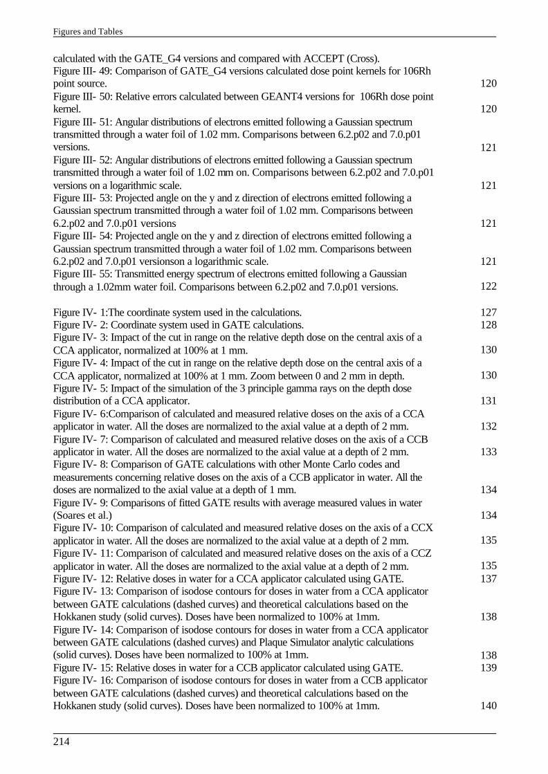
Figures and Tables
214
calculated with the GATE_G4 versions and compared with ACCEPT (Cross). Figure III- 49: Comparison of GATE_G4 versions calculated dose point kernels for 106Rh point source. 120 Figure III- 50: Relative errors calculated between GEANT4 versions for 106Rh dose point kernel. 120 Figure III- 51: Angular distributions of electrons emitted following a Gaussian spectrum transmitted through a water foil of 1.02 mm. Comparisons between 6.2.p02 and 7.0.p01 versions. 121 Figure III- 52: Angular distributions of electrons emitted following a Gaussian spectrum transmitted through a water foil of 1.02 mm on. Comparisons between 6.2.p02 and 7.0.p01 versions on a logarithmic scale. 121 Figure III- 53: Projected angle on the y and z direction of electrons emitted following a Gaussian spectrum transmitted through a water foil of 1.02 mm. Comparisons between 6.2.p02 and 7.0.p01 versions 121 Figure III- 54: Projected angle on the y and z direction of electrons emitted following a Gaussian spectrum transmitted through a water foil of 1.02 mm. Comparisons between 6.2.p02 and 7.0.p01 versionson a logarithmic scale. 121 Figure III- 55: Transmitted energy spectrum of electrons emitted following a Gaussian through a 1.02mm water foil. Comparisons between 6.2.p02 and 7.0.p01 versions. 122 Figure IV- 1:The coordinate system used in the calculations. 127 Figure IV- 2: Coordinate system used in GATE calculations. 128 Figure IV- 3: Impact of the cut in range on the relative depth dose on the central axis of a CCA applicator, normalized at 100% at 1 mm. 130 Figure IV- 4: Impact of the cut in range on the relative depth dose on the central axis of a CCA applicator, normalized at 100% at 1 mm. Zoom between 0 and 2 mm in depth. 130 Figure IV- 5: Impact of the simulation of the 3 principle gamma rays on the depth dose distribution of a CCA applicator. 131 Figure IV- 6:Comparison of calculated and measured relative doses on the axis of a CCA applicator in water. All the doses are normalized to the axial value at a depth of 2 mm. 132 Figure IV- 7: Comparison of calculated and measured relative doses on the axis of a CCB applicator in water. All the doses are normalized to the axial value at a depth of 2 mm. 133 Figure IV- 8: Comparison of GATE calculations with other Monte Carlo codes and measurements concerning relative doses on the axis of a CCB applicator in water. All the doses are normalized to the axial value at a depth of 1 mm. 134 Figure IV- 9: Comparisons of fitted GATE results with average measured values in water (Soares et al.) 134 Figure IV- 10: Comparison of calculated and measured relative doses on the axis of a CCX applicator in water. All the doses are normalized to the axial value at a depth of 2 mm. 135 Figure IV- 11: Comparison of calculated and measured relative doses on the axis of a CCZ applicator in water. All the doses are normalized to the axial value at a depth of 2 mm. 135 Figure IV- 12: Relative doses in water for a CCA applicator calculated using GATE. 137 Figure IV- 13: Comparison of isodose contours for doses in water from a CCA applicator between GATE calculations (dashed curves) and theoretical calculations based on the Hokkanen study (solid curves). Doses have been normalized to 100% at 1mm. 138 Figure IV- 14: Comparison of isodose contours for doses in water from a CCA applicator between GATE calculations (dashed curves) and Plaque Simulator analytic calculations (solid curves). Doses have been normalized to 100% at 1mm. 138 Figure IV- 15: Relative doses in water for a CCB applicator calculated using GATE. 139 Figure IV- 16: Comparison of isodose contours for doses in water from a CCB applicator between GATE calculations (dashed curves) and theoretical calculations based on the Hokkanen study (solid curves). Doses have been normalized to 100% at 1mm. 140
Figures and Tables
215
Figure IV- 17: Comparison of isodose contours for doses in water from a CCB applicator between GATE calculations (dashed curves) and Plaque Simulator analytic calculations (solid curves). Doses have been normalized to 100% at 1mm. 140 Figure IV- 18: Comparison of isodose contours for doses in water from a CCB applicator between GATE calculations (dashed curves) and ACCEPT 3.0 calculations from Cross et al. (solid curves). Doses have been normalized to 100% at 1mm. 141 Figure IV- 19: Relative doses in water for a CCX applicator calculated using GATE. 141 Figure IV- 20: Comparison of isodose contours for doses in water from a CCX applicator between GATE calculations (dashed curves) and theoretical calculations based on the Hokkanen study (solid curves). Doses have been normalized to 100% at 1mm. 142 Figure IV- 21: Comparison of isodose contours for doses in water from a CCX applicator between GATE calculations (dashed curves) and Plaque Simulator analytic calculations (solid curves). Doses have been normalized to 100% at 1mm. 143 Figure IV- 22: Relative doses in water for a CCZ applicator calculated using GATE. 143 Figure IV- 23: Comparison of isodose contours for doses in water from a CCZ applicator between GATE calculations (dashed curves) and theoretical calculations based on the Hokkanen study (solid curves). Doses have been normalized to 100% at 1mm. 144 Figure IV- 24: Comparison of isodose contours for doses in water from a CCZ applicator directly against the “eye” between GATE calculations (dashed curves) and Plaque Simulator analytic calculations (solid curves). Doses have been normalized to 100% at 1mm. 145 Figure IV- 25: Phantom Model 062 from CIRS compagny. 148 Figure IV- 26:Schema of the phantom inserts with their composition and placement. 149 Figure IV- 27:Calculated versus measured Hounsfield units of the phantom inserts (values listed in Table IV- 16). 150 Figure IV- 28:Mass density versus CT number in the range of skeletal tissues. The plot shows the data points of the skeletal tissues from Table IV- 18 together with the interpolation function. 153 Figure IV- 29:CT number versus elemental weights in the range of skeletal tissues. The plot shows the data points of the skeletal tissues together with the interpolation functions corresponding to Equation IV-18: (a) hydrogen (H) and nitrogen (N), (b) carbon (C) and oxygen (O), (c) phosphorus (P) and calcium (Ca). 154 Figure IV- 30: CT number versus mass density in the range of soft tissues. The data points of the tissues from Table IV- 17 are plotted together with the interpolation functions according to Equation IV-19 and Equation IV-21. 156 Figure IV- 31: CT number versus elemental weights in the range of soft tissues. For each of the elements (a) hydrogen and nitrogen, (b) carbon and oxygen, the data points of the tissues from Table IV- 17 are plotted together with the interpolation Equation IV-20 and Equation IV-22. 157 Figure IV- 32: Conversion of CT number to mass density. Equation IV-19 and Equation IV-21 are used for the range between –86 and 105 Hounsfield units. Above 105H, Equation IV-17 is applied. In the range between –1000 and –86 H, the mass densities of air and adipose tissue 3 are interpolated by a straight line. 158 Figure IV- 33: CIRS phantom image. In red, has been highlighted the bins –22 to 7 H. 159 Figure IV- 34: CIRS phantom image. In red, has been highlighted the bins 19 to 80 H. 159 Figure IV- 35: Brain image. In red has been highlighted the bin 19 to 80 H. 159 Figure IV- 36: Brain image. In red has been highlighted the bin 80 to 120 H. 159 Figure IV- 37: Mediastin image. In red has been highlighted the bin –950 to –120 H. 160 Figure IV- 38: Comparisons of dose distributions of a 6 MeV electron beam in Urine, Skin1 and Mat-19-80 tissues. 161 Figure IV- 39: Comparisons of dose distributions of a 21 MeV electron beam in Urine, Skin1 and Mat-19-80 tissues. 161 Figure IV- 40: Comparisons of dose distributions of a 25 MeV photon beam in Urine, Skin1 and Mat-19-80 tissues.
162
Figures and Tables
216
and Mat-19-80 tissues. Figure IV- 41: Relative deviations between dose distributions in the three media: (a) between Urine and Mat-19-80 for 6 and 21 MeV electron beams, (b) between Skin1 and Mat-19-80 for 6 and 21 MeV electron beams, (c) presents deviations for 25 MeV photons beams. 163 Figure IV- 42: Comparisons of dose distributions of a 6 MeV electron beam in Mat-300-400, Mean Bone and Mat-1500-1600 tissues. 164 Figure IV- 43: Comparisons of dose distributions of a 21 MeV electron beam in Mat-300-400, Mean Bone and Mat-1500-1600 tissues. 164 Figure IV- 44: Comparisons of dose distributions of a 25 MeV photon beam in Mat-300-400, Mean Bone and Mat-1500-1600 tissues. 165 Figure V- 1: The Leap Frog method (with 4 parallel processes) 171 Figure V- 2: The Sequence Splitting method (with 4 parallel processes) 172 Figure V- 3: The Independent Sequences method (with 4 parallel processes) 172 Figure V- 4: Consumption in pseudorandom numbers for different Monte Carlo simulations 174 Figure V- 5: Consumption in pseudorandom numbers per particle for different Monte Carlo simulations 174 Figure V- 6: Schema of the jobs management with JJS on a grid environment 175 Figure V- 7: Prototype web portal algorithmic schema. 177 Figure V- 8: A web portal prototype for the parallelisation and submission of GATE simulations on the EDG testbed. 177 Figure V- 9: Energy spectrum of a capillary source of 20 MBq of 99mTc 178 Figure V- 10: Comparison of relative deposit doses along the central axis of the eye using a local and a parallel computation 179 Figure V- 11: Influence of the number of threads in parallel launchings 180 Figure V- 12: Comparison of computing time between a local and a parallel submission 180 Figure V- 13: Influence of the launching time in parallel launching 181 Figure V- 14: Launching times of a set of 100 jobs at CC-IN2P3 grid site over a period of 22 days. 182 Figure V- 15: Total computing times of a set of 100 jobs at CC-IN2P3 grid site over a period of 22 days. 182 Figure V- 16: Time per status for different simulation parts on the CCIN2P3 site. 184 Figure V- 17: Time per status for different simulation parts on the LPC site. 184 Figure V- 18: Comparison of computing time between a local and a parallel submission on the CCIN2P3 site. 185 Figure V- 19: Comparison of computing time between a local and a parallel submission on the LPC site 185 Figure V- 20: Three-tier architecture of the GENIUS portal 187 Figure V- 21: Screenshot of the web portal Genius. The connexion to the Grid using the user’s MyProxy Passphrase. 189 Figure V- 22: Screenshot of the web portal Genius. GATE applications for biomed VO services. 189 Figure V- 23: Algorithmic schema of the gategrid.sh file. 190 Figure V- 24: Screenshot of the web portal Genius.The creation of the GATE files. 192 Figure V- 25: Screenshot of the web portal Genius. The selection of the status files. 192 Figure V- 26: Script template (script.sh) to launch GATE simulations 193 Figure V- 27: Script file created automatically by the GENIUS portal from the script template 193 Figure V- 28: Screenshot of the web portal Genius. The creation of the jdl files. 194 Figure V- 29: JDL template part1 (gate_job.jdl.template) 194 Figure V- 30: JDL template part 2 (gate_job.jdl.template.last) 194 Figure V- 31: Example of a JDL file created by the GENIUS web portal 195 Figure V- 32: Resource Broker configuration file. 196
Figures and Tables
217
Figure V- 33: Resource Broker and VO configuration file. 196 Figure V- 34: Screenshot of the web portal Genius. The choice of the CE resources. 196 Figure V- 35: Screenshot of the web portal Genius. Visualisation of the status of the jobs. 197 Figure V- 36: Screenshot of the web portal Genius. Retrieval of jobs outputs when each job has the status Done with an Exit code 0. 198 Figure V- 37: Screenshot of the web portal Genius. Visualization of the output directories. 198 Figure V- 38: Screenshot of the web portal Genius. Visualization of the ocular brachytherapy isodoses. 199 Figure V- 39: Test of computing time obtained on different computer: PC AMD, IBM SP4 (32 bits), IBM SP4 (64 bits), SGI ALTIX 3700 (64 bits), SGI ORIGIN 3800 and CRAY XD1.
200
Tables Table I- 1: Beta emisions of 106Ru/106Rh nuclide 16 Table I- 2: Photon emissions of 106Rh nuclide 16 Table I- 3: Beta energy spectrum of 106Rh 16 Table I- 4: Description of the BEBIG ophthalmic applicators 17 Table I- 5: Water-equivalent plastics used for dosimetric measurements. 29 Table I- 6: Conversion factor F(type,z) depending on plaque type and distance z from the inner concave plaque surface along the central axis. 33 Table II- 1: Biomed CEs resources 63 Table II- 2: Biomed SEs resources 63 Table II- 3: Biomed RBs, RLS and LDAP resources 64 Table II- 4: Queue configuration at LPC site (maximum CPU time, Wall time and running jobs) 66 Table II- 5: Queue mean running time in seconds at LPC, corresponding Standard Deviation and Coefficient of Variation. 66 Table II- 6: Queue mean waiting time in seconds at LPC, corresponding Standard Deviation, Coefficient of Variation and number of jobs. 66 Table II- 7: Group interarrival time in seconds, corresponding Standard Deviation and 67 Table II- 8: EGEE South West Resources. 69 Table III- 1: Service Object Pair classes 80 Table III- 2: Organisation of DICOM flow 81 Table III- 3: The five paths with their respective weight. The sum of weights: 0.25+0.25+0.125=1. 91 Table III- 4: File table.visu. The color Red (255 0 0) has been assigned to the material Mat19-80 (for Hounsfield number between 19 and 80 H) 93 Table III- 5: Electron CSDA ranges, rE, in water 107 Table IV- 1: q and j angles defining the ophthalmic plaques. 128 Table IV- 2: Ratios of normalized doses on the central axis of a CCA plaque. 136 Table IV- 3: Ratios of normalized doses on the central axis of a CCB plaque. 136 Table IV- 4: Ratios of normalized doses on the central axis of a CCX plaque. 136 Table IV- 5: Ratios of normalized doses on the central axis of a CCZ plaque. 136 Table IV- 6: Ratio of doses from GATE to analytical point kernels from Hokkanen method for a CCA applicator. 137 Table IV- 7: Ratio of doses from GATE to Plaque Simulator calculations for a CCA applicator. 138 Table IV- 8: Ratio of doses from GATE to analytical point kernels from Hokkanen method for a CCB applicator.
139
Figures and Tables
218
for a CCB applicator. Table IV- 9: Ratio of doses from GATE to Plaque Simulator calculations for a CCB applicator. 140 Table IV- 10: Ratio of doses from GATE to analytical point kernels from Hokkanen method for a CCX applicator. 142 Table IV- 11: Ratio of doses from GATE to Plaque Simulator calculations for a CCX applicator. 142 Table IV- 12: Ratio of doses from GATE to analytical point kernels from Hokkanen method for a CCZ applicator. 144 Table IV- 13: Ratio of doses from GATE to Plaque Simulator for a CCZ applicator. 144 Table IV- 14: Comparisons of relative differences between GATE with Plaque Simulator and point kernel integration at 2 mm and 4 mm off the central axis and 3 mm in depth. 145 Table IV- 15: Mass-density and chemical composition of the 10 phantom materials used for the determination of k1 and k2 values (the titanium insert hasn’t been used for the measurements). 148 Table IV- 16:CT numbers of the phantom inserts. The values H(meas.) are measured on a General Electric LightSpeed 16Pro CT scanner with a tube voltage of 120 kV. The values H (calc.) are calculated by means of Equation IV? 11 with values k1=1.51 ´ 10-4 and k2= 2.78 ´ 10-5 149 Table IV- 17:Calculated CT numbers, mass-density and elemental weights of soft tissues. The tissue parameters are taken from Woodard and White (1986), the Hounsfield units are calculated using equations X and Y. In the column others are combined the elements Na, Mg, S, Cl, K and Fe. 151 Table IV- 18:Calculated CT numbers, mass-density and elemental weights of skeletal tissues. The tissue parameters are taken from White et al. (1987) and Woodward and White (1986), the Hounsfield units are calculated using equations X and Y. In the column others are combined the elements Na, Mg, S, Cl, K and Fe. 152 Table IV- 19: Conversion of CT numbers to elemental weights. The scale of Hounsfield units is divided into 24 bins. The first bin from –1000 to –950 H is assigned to the composition of air, the next bin up to –120 H with the composition of lung. The following five bins up to 18 H form a step function corresponding to Equation IV? 20. Between 19 and 80 H the mean values of all tissues within this range are used. The composition of connective tissue (H=105) is assigned to the bin between 80 and 120 H. All bins above 120 Hounsfield units form a step function corresponding to Equation IV? 18.
158
Table IV- 20: Mass-density and elemental weights of media used in GATE Monte Carlo simulations.
160
Table V- 1: Speedup for different jobs submission 181 Table V- 2: Speedup calculations for Total computing times of a set of 100 jobs at CC-IN2P3 grid site over a period of 22 days
182
Table V- 3: Sequential versus grid computation time on CCIN2P3 site. 185 Table V- 4: Sequential versus grid computation time on LPC site. 185
Publications and other work
219
Publications and other work PUBLICATIONS
L.Maigne, D. Hill, P. Calvat, V. Breton, R. Reuillon, D.Lazaro, Y. Legré, D. Donnarieix, "Parallelization of Monte Carlo Simulations and Submission to a Grid Environment", Parallel Processing Letters journal, Vol. 14, No. 2 (June 2004), p 177-196.
S. Jan, G. Santin, D. Strul, S. Staelens, K. Assié, D. Autret, S. Avner, R. Barbier, M. Bardiès, P.M. Bloomfield, D. Brasse, V. Breton, P. Bruyndonckx, I. Buvat, A.F. Chatziioannou, Y. Choi, Y.H. Chung, C.Comtat, D.Donnarieix, L.Ferrer, S.J. Glick, C.J. Groiselle, D. Guez, P.-F. Honoré, S. Kerhoas-Cavata, A.S. Kirov, V. Kohli, M. Koole, M. Krieger, D.J. van der Laan, F. Lamare, G. Largeron, C. Lartizien, D. Lazaro, M.C. Maas, L. Maigne, F. Mayet, F. Melot, C. Merheb, E. Pennacchio, J. Perez, U. Pietrzyk, F.R. Rannou, M. Rey, D.R. Schaart, C.R. Schmidtlein, L. Simon, T.Y. Song, J.-M. Vieira, D. Visvikis, R. van de Walle, E. Wieërs, and C. Morel, “GATE: a simulation toolkit for PET and SPECT”, Phys. Med. Biol., 49 (2004) 4543-4561.
J. Montagnat, F. Bellet, H. Benoit-Cattin, V. Breton, L. Brunie, H. Duque, Y. Legré, I.E. Magnin, L. Maigne, S. Miguet, J.-M. Pierson, L. Seitz, T. Tweed, “Medical images simulations, storage, and processing, on the European DataGrid testbed”, Journal of Grid Computing, 2004.
D. Lazaro, I. Buvat, G. Loudos, D. Strul, G. Santin, N. Giokaris, D. Donnarieix, L. Maigne, V. Spanoudaki, S. Styliaris, S. Staelens and V. Breton, “Monte Carlo simulation of a CsI(Tl) gamma camera dedicated to small animal imaging using GATE”, Phys. Med. Biol., 49 271-285, 2004.
L. Maigne co-author part of the HealthGrid White Paper collaboration, “The HealthGrid White Paper”: chapter 4 on Computational Models of the Human Body, From Grid to Healthgrid, Studies in Health Technology and Informatics (vol. 112) IOS Press ISBN: 1-58603-510-X.
V. Breton, C. Blanchet, Y. Legré, L. Maigne & J. Montagnat, “Grid technology to biomedical applications”, Proceedings of High Performance Computing for Computational Science, VECPAR 2004 conference, Lecture Notes in Computer Science vol 3402 , edition Springer (2005) 204-218.
Publications and other work
220
CONFERENCES
L. Maigne, D. Donnarieix, V. Breton, Y. Legré, “Use of a calculation grid to run Monte Carlo simulation programs with the Geant4 Software in ocular brachytherapy”, Physica Medica, Vol. XIX, N°3, July-September 2003.
L. Berger, V. Breton, D. Donnarieix, D. Lazaro, L. Maigne, “Computation of P1 problem using the Monte Carlo code GATE” in Intercomparison on the usage of computational codes in radiation dosimetry, QUADOS Conference proceedings G. Gualdrini and P. Ferrari Editors, 2004.
D. Visvikis, M. Bardiès, S. Chiavassa, C. Danford, A. Kirov, F. Lamare, L. Maigne, S. Staelens, R. Taschereau, “Use of the GATE Monte Carlo package for dosimetry applications”, ITBS 2005 conference, to be published in NIMA journal.
S. Staelens, J. De Beenhouwer, D. Kruecker, L. Maigne, F. Rannou, L. Ferrer, Y. D’Asseler, I. Buvat, I. Lemahieu, “GATE: improving the computational efficiency”, ITBS 2005 conference, to be published in NIMA journal.


Abstract Although often quite time consuming, Monte Carlo method is the calculation algorithm that most closely models the actual physics of the energy deposition process. The idea is to use Monte Carlo calculations in daily cancer treatment using radiation to compete with treatment planning systems (TPS) in the delivering of absorbed dose to tumour for specific treatments. To achieve this goal, two points have been particularly studied in this thesis: the validation of the GATE platform for dosimetry applications using electrons, with a specific study concerning ocular brachytherapy treatments using 106Ru/106Rh ophthalmic applicators and the deployment of GATE simulations in a grid environment to reduce the very high computation time of those simulations. Monoenergetic and polyenergetic electron dose point kernels have been simulated using the GATE platform and compared with other Monte Carlo codes. Three versions of the GEANT4 physics package have been used for the comparisons (5.2, 6.2 and 7.0). Results show that the Multiple Scattering implementation is responsible for the discrepancies observed between the codes. Simulations of ocular brachytherapy treatments compared with Monte Carlo and measurements show a good agreement. The transcription of Hounsfie ld units from CT images of patient’s anatomy to tissue parameters is the other work presented for a next usage of GATE on voxelized images for personnalized dosimetry. The DataGrid and then the EGEE infrastructures were used to deploy GATE simulations to reduce their computation time in order to use them in clinical practice. The method used to parallelize the GATE simulations is the splitting of the random number generator (RNG) into independent sequences. Computing time tests performed on the grid testbeds show that a significant speed-up is obtained. Functionalities to split, launch and monitor GATE simulations on a grid infrastructure have been implemented on the GENIUS web portal. A first prototype of this portal is accessible from hospital to use the accurate Monte Carlo algorithms in a transparent and secure way for ocular cancer treatments. Keywords: GATE, GEANT4, EGEE, grid, Monte Carlo simulations, dosimetry, ocular brachytherapy, CT numbers.
Résumé Bien que souvent assez consommatrice en temps de calcul, la méthode Monte Carlo est l’algorithme de calcul qui modélise au plus près la physique liée aux processus de dépôts d’énergie. L’idée est d’utiliser les calculs Monte Carlo dans le traitement quotidien du cancer par rayonnement pour rivaliser avec les systèmes de planification de traitement (TPS) existants dans le but de délivrer une dose absorbée à la tumeur pour des traitements spécifiques. Pour atteindre cet objectif, deux points ont été particulièrement étudiés au cours de cette thèse : la validation de la plate-forme de simulation GATE pour des applications en dosimétrie utilisant des électrons, une étude particulière est faite concernant les traitements de curiethérapie oculaire utilisant des applicateurs ophtalmiques de 106Ru/106Rh, et le déploiement des simulations GATE dans un environnement de grille pour réduire les temps de calcul très élevés de ces simulations. Des points kernels de dose d’électrons mono-énergétiques et poly-énergétiques ont été simulés en utilisant la plate-forme GATE et comparés à d’autres codes Monte Carlo. Trois versions des packages de librairies ont été utilisées pour les comparaisons (5.2, 6.2 et 7.0). Les résultats montrent que l’implémentation de la diffusion multiple est responsable des différences observées e ntre les codes. Les simulations de traitements de curiethérapie oculaire comparées avec d’autres Monte Carlo et des mesures montrent un bon accord. La transcription des unités Hounsfield, à partir des données scanner sur l’anatomie du patient, en paramètre s tissulaires est l’autre étude présentée pour une utilisation prochaine de GATE sur des images voxélisées pour la dosimétrie personnalisée. Les infrastructures des projets DataGrid puis d’EGEE ont été utilisées pour déployer les simulations GATE afin de réduire leur temps de calcul dans le but de les utiliser en routine clinique. La méthode utilisée pour paralléliser les simulations GATE est la division du générateur de nombres aléatoires (RNG) en séquences indépendantes. Des tests de temps de calcul réalisés sur des bancs tests de grille montrent qu’un gain significatif est obtenu. Les fonctionnalités pour diviser, lancer et contrôler les simulations GATE sur une infrastructure de grille ont été implémentées sur le portail web GENIUS. Un premier prototype de ce portail est accessible à partir d’un centre hospitalier pour l’utilisation de la précision des algorithmes Monte Carlo de manière transparente et sécurisée pour des traitements de cancer de l’œil. Mots clés : GATE, GEANT4, EGEE, grille de calcul, simulations Monte Carlo, dosimétrie, curiethérapie oculaire, nombres Hounsfield.