Embed Size (px)
Citation preview


DEPARTMENT OF THE INTERIOR
BRUCE BABBITT, Secretary
U.S. GEOLOGICAL SURVEY
Dallas L. Peck, Director
Any use of trade, product, or firm names in this publication is for descriptive purposes only and does not imply endorsement
by the U.S. Government
Manuscript approved for publication, March 22, 1993
Text and illustrations edited by George A. Havach
Library of Congress Cataloging in Publication Data
The Loma Prieta, California, earthquake of October 17, 1989. (U.S. Geological Survey professional paper ; 1550) Includes bibliographical references. Contents: Earthquake occurrence / Malcom J.S. Johnston, editor ; William H. Bakun and William H. Prescott,
coordinators. ch. C. Preseismic observations. -Strong ground motion and ground failure / Thomas D. O'Rourke, editor ; Thomas L. Holzer, coordinator. ch. F. Marina District.
1. EarthquakesÑCalifornia-Lom Prieta Region. 2. EarthquakesÑCalifornia-Sa Francisco Bay Area. I. Series. QE535.2U6L66 1992 55 1.2'2'097946 92-32287
For sale by the Book and Open-File Report Sales, U.S. Geological Survey, Federal Center, Box 25286, Denver, CO 80225

SAN ANDREAS FAULT
SAN ANDREAS FAULT
MAGNETOMETER
SEISMOMETER - WATER WELL
TOP-Distortion in the Pacific and North American plates centered about the San Andreas fault due to the relentless plate move- ment, showing instruments used to monitor this distortion and the earthquakes that result from it. BOTTOM-Three-dimensional view of changes in elevation and horizontal displacement due to 1.1 m of oblique slip on ction of 7 the San Andreas fault that failed during the Loma Prieta earthquake. Although fault slip did not reach the Earth's surface, intense accelerations from the earthquake generated a complex series of surface cracks, fractures, and landslides around the epicentral region.

CONTENTS
Seismicity in the southern Santa Cruz Mountains during the 20-year period before the earthquake --------------
By Jean A. Olson and David P. Hill
Analysis of low-frequency-electromagnetic-field measurements near the epicenter ........................
By Anthony C. Fraser-Smith, Arrnan Bernardi, Robert A. Helliwell, Paul R. McGill, and O.G. Villard, Jr.
Seismomagnetic effects ........................................ By Robert J. Mueller and Malcolm J.S. Johnston
Near-field high-resolution strain measurements ------------ By Malcolm J.S. Johnston and Alan T. Linde
No convincing precursory geodetic anomaly observed --- By Michael Lisowski, James C. Savage, William H. Prescott,
Jerry L. Svarc, and Mark H. Murray
Detection of hydrothermal precursors to large northern California earthquakes ............................. -------
By Paul G. Silver, Natalie J. Valette-Silver, and Olga Kolbek
Borehole strain measurements of solid-earth-tidal amplitudes---------------------------------------------------
By Alan T. Linde, Michael T. Gladwin, and Malcolm J.S. Johnston
Page
Cl
3
17
27
31
47
53
59
67
73
81

THE LOMA PRIETA, CALIFORNIA, EARTHQUAKE OF OCTOBER 17,1989: EARTHQUAKE OCCURRENCE
PRESEISMIC OBSERVATIONS
INTRODUCTION
By Malcolm J.S. Johnston, U.S. Geological Survey
The October 17, 1989, Loma Prieta, Calif., Mc=7.1 earthquake (see U.S. Geological Survey staff, 1990, for general description) provided the first, opportunity in the history of fault monitoring in the United States to gather multidisciplinary preearthquake data in the near field of an M=7 earthquake. The data obtained include observations on seismicity, continuous strain, long-term ground dis- placement, magnetic field, and hydrology. The papers in this chapter describe these data, their implications for fault-failure mechanisms, the scale of prerupture nucle- ation, and earthquake prediction in general.
Of the 10 papers presented here, about half identify preearthquake anomalies in the data, but some of these re- sults are equivocal. Seismicity in the Loma Prieta region during the 20 years leading up to the earthquake was unre- markable (see Olson and Hill, this chapter). In retrospect, however, it is apparent that the principal southwest-dip- ping segment of the subsequent Loma Prieta rupture was virtually aseismic during this period. Two M=5 earth- quakes did occur near Lake Elsman near the junction of the Sargent and San Andreas faults within 2.5 and 15 months of, and 10 km to the north of, the Loma Prieta epicenter. Although these earthquakes were not on the sub- sequent rupture plane of the Loma Prieta earthquake and other M=5 earthquakes occurred in the preceding 25 years, it is now generally accepted that these events were, in some way, foreshocks to the main event.
The most intriguing observations were of increased ul- tra-low-frequency (ULF) magnetic noise near Corralitos, Calif. (see Fraser-Smith and others, this chapter), during the weeks to months before the earthquake and the months after the earthquake. These observations seem restricted to the frequency band 0.0 1-1 0 Hz because lower-frequency noise was not observed at 0.001 Hz at reactivated magne- tometer monitoring sites near Corralitos, Calif. (see Muel- ler and Johnston, this chapter). The observations raise several issues regarding a causative physical mechanism for these signals. Seismic signals also recorded near Cor- ralitos in the frequency band 0.1-10 Hz (see White and Ellsworth, this chapter) show no indication of increased noise, nor do strain signals at more distant sites (see
Johnston and Linde, this chapter). The four most likely physical mechanisms that could generate these signals in the hypocentral region are (1) dynamic changes in electri- cal conductivity due to strain-driven crack opening and closure; (2) dynamic charge generation due to strain, hy- drodynamic, and gas-dynamic processes; (3) electrokinetic effects due to dynamic pore-pressure variations; and (4) pi- ezomagnetic effects resulting from pore-pressure-driven stress changes modifying the magnetic properties of crustal rocks. The absence of detectable seismic or strain signals on nearby seismometers and borehole strainmeters at the 10-pmls and 10-"Is levels, respectively, strongly limits the size (that is, moment) of the source region driving the above-mentioned mechanisms.
Gladwin and others (this chapter) report possible precur- sory changes in shear-strain rate in a direction parallel to the San Andreas fault, as determined on a three-component borehole strainmeter some 40 km southeast of the epicen- ter. Although there initially was some support for these ob- servations in measurements of geodetic lines across the epicentral region (see Lisowski and others, 1990), more careful processing of these data indicates that this support was marginal and that no convincing geodetic anomaly was observed on geodetic lines crossing the epicentral re- gion before the Loma Prieta earthquake (see Lisowski and others, this chapter).
Another intriguing observation is the report of changes in streamflow from streams to the north of the epicenter (see Roeloffs, this chapter). Although this report seems un- equivocal, any associated changes in strain appear to have been limited in extent, because no change greater than about 1 microstrain was observed on the borehole strain- meter to the south of the epicentral region during this time (see Johnston and others, this chapter). Observations of changes in geyser activity at Calistoga, Calif., some 177 krn from the epicenter (see Silver and others, this chapter), are difficult to explain, particularly when high-quality strain measurements only several tens of kilometers from the epicenter were uneventful and changes in material properties, as indicated by the response to earth tides, were absent (see Linde and others, this chapter).

2 PRESEISMIC 0
REFERENCES CITED Lisowski, Michael, Prescott, W.H., savage, J.C., and Svarc, J.L., 1990, A
possible geodetic anomaly observed prior to the Lorna Prieta, Cali-
fornia, earthquake: Geophysical Research Letters, v. 17, no. 8, p. 1211-1214.
U.S. Geological Survey staff, 1990, The Lorna Prieta, California, earth- quake; an anticipated event: Science, v. 247, no. 4940, p. 286-293.
THE LOMA PRIETA, CALIFORNIA, EARTHQUAKE OF OCTOBER 17,1989: EARTHQUAKE OCCURRENCE
PRESEISMIC OBSERVATIONS
SEISMICITY IN THE SOUTHERN SANTA CRUZ MOUNTAINS DURING THE 20-YEAR PERIOD BEFORE THE EARTHQUAKE
CONTENTS
By Jean A. Olson and David P. Hill, U.S. Geological Survey
Page
C3 3 4 6 6
10 11 12 12
14 15 15 15
cause they occurred within 16 and 2% months, respectively, of the Loma Prieta earthquake. In the 25 years before the earthquake, however, two other M=5 events occurred along the Loma Prieta rupture zone: the 1964 (M=5.0) and 1967 (M=5.3) Corralitos earthquakes, located approximately 17 km east and 10 km southeast, respectively, of the Loma Prieta main shock. In view of these other M=5 events along the rupture zone, the temporal proximity of the Lake Elsman earthquakes and the Loma Prieta earthquake may be coincidental and not necessarily precursory. Thus, with the possible exception of the Lake Elsman earthquakes, seismicity patterns in the 20-year period before the Loma Prieta earthquake were essentially stable, showing no clear precursory changes.
INTRODUCTION ABSTRACT
We examine the spatial distribution of well-located earthquakes in the 20-year period before the earthquake, and their association with faults, along a 100-km-long ex- tent of the southern Santa Cruz Mountains. Several faults in the study area are clearly associated with background seismicity since 1969. Notably, however, the principal southwest-dipping part of the Loma Prieta rupture below 10-km depth was virtually aseismic. Most of the seismici- ty in the study area was associated with the creeping sec- tion of the San Andreas fault south of Pajaro Gap and adjacent faults to the east. However, the area centered 11 km north-northeast of the Loma Prieta main shock, near the intersection of the San Andreas and Sargent fault trac- es, also produced persistent seismicity, albeit at a much lower rate. This seismicity includes the 1988 (M=5.3) and 1989 (M=5.4) Lake Elsman earthquakes, which have fault- plane solutions consistent with oblique strike-slip and re- verse-slip components on a plane that dips about 65' NE. These events stand out against the background seismicity because they are a full unit of magnitude larger than other events within a 15-km radius for at least 74 years and be-
The October 17, 1989, Loma Prieta earthquake was the first major (Ms7) earthquake to occur anywhere along the main branch of the San Andreas fault zone since the great (M=8) San Francisco earthquake of 1906. Because the Loma Prieta earthquake occurred within the confines of the U.S. Geological Survey's (USGS) dense, regional seismic network that began operation in the late 1960's (Eaton, 1989), we have an exceptional record of well-located mi- croearthquakes in the preceding 20 years. In this paper, we document the spatiotemporal distribution of microearth- quakes from 1969 up to the time of the Loma Prieta earth- quake. Two noteworthy aspects of this preearthquake seismicity are that (1) the southwest-dipping part of the Loma Prieta rupture below 10-km depth was virtually qui- escent in the 20-year period before the earthquake, and (2) only two earthquakes stand out as unusual in this period: the 1988 (M=5.3) and 1989 (M=5.4) Lake Elsman earth- quakes, located 10 and 12 km, respectively, north-northeast of the Loma Prieta main shock. The record of Ms5 earth- quakes since 1910, however, includes two other M=5 events: the 1964 (M=5.0) and 1967 (M=5.3) Corralitos

c 4 PRESEISMIC OBSERVATIONS
earthquakes, located approximately 17 km east and 10 km southeast, respectively, of the Loma Prieta main shock.
Previous retrospective studies using data from the USGS' Central California Seismic Network (Calnet) to fo- cus on seismicity patterns along the San Andreas fault zone through the the Santa Cruz Mountains before the earthquake include those by King and others (1990), 01- son (1990), and Seeber and Arrnbruster (1990). Ellsworth (1990) and Hill and others (1990, 1991) provided an over- view of the seismotectonic fabric and earthquake history of the San Andreas fault system and extensive references to related studies.
38'
SEISMOTECTONIC SETTING
The San Andreas fault system in central California ac- commodates the relative motion between the Pacific and North American plates by right-lateral, strike-slip displace- ment distributed along several subparallel branches (fig. 1). The main branch, which cuts through the Santa Cruz Mountains and the San Francisco peninsula with a north- westward strike, juxtaposes Cretaceous granitic basement of the Salinian block on the west against melange of the Mesozoic Franciscan Complex and the Great Valley se- quence on the east, with a demonstrated post-Miocene off-
0 10 20 30 40 50 KILOMETERS I I 1 I I I
\ MAGNITUDES
Figure 1.-Santa Cruz Mountains area, Calif., showing locations of epicenters of (A) preearthquake events of Mzl.5 since January 1, 1969 (G.m.t.), and (B) events of Mil.5 between October 18 and December 31, 1989 (G.m.t.), including Loma Prieta main shock and aftershocks. Rectangle delimits study area. CF, Concord fault; GVF, Green Valley fault; SF, San Francisco.

SEISMICITY IN THE SOUTHERN SANTA CRUZ MOUNTAINS DURING THE 20-YEAR PERIOD BEFORE THE EARTHQUAKE CS
set of more than 300 km (Irwin, 1990). To the west, the San Gregorio fault skims the coast of the peninsula and merges with the principal branch of the San Andreas fault north of the Golden Gate near Bolinas Bay (fig. 1B). To the east, the Calaveras fault splays northward into the Hayward, Calaveras, and Green Valley-Concord faults.
The sections of the San Andreas fault system marked by dense lineations of epicenters in figure 1A show evidence of active fault creep. The central, creeping section of the main branch, which extends from the latitude of Pajaro Gap for 200 km to the southeast (see Hill and others, 1991), has a maximum, long-term creep rate of 30 m d y r in the central part of this section, close to the geodetically derived rate of 33 mm/yr measured across a 60-km-wide zone (Thatcher, 1990). Thus, along the central part of this creeping section, creep accommodates most of the slip, and the crustal blocks on either side of the fault are accu- mulating little, if any, shear strain (Thatcher, 1990). Active fault creep, however, is partially shunted to the north along the Calaveras-Hayward fault system; and the creep rate along the section of the San Andreas fault south of Pajaro Gap and its junction with the Calaveras fault ranges from 8 to 14 m d y r (Burford and Harsh, 1980; Schulz and others, 1982). Creep rates along the Calaveras-Hayward branches also diminish northward, from 13 mrnlyr along the southern section of the Calaveras fault to 3-6 m d y r along the northern sections of the Calaveras and Hayward faults, respectively (see Thatcher, 1990).
In contrast, the section of the fault that ruptured in the 1906 earthquake produces only sparsely scattered micro- earthquake activity and no fault creep. This section of the fault extends for more than 300 km between the north end of the creeping section along the main branch near Pajaro Gap and Cape Mendocino (see Hill and others, 1991). Be- fore the Loma Prieta earthquake, geodetic measurements indicated that this entire section of the fault was locked
since the 1906 earthquake and that shear strain was accu- mulating in the crustal blocks on either side of the fault (Thatcher, 1990).
The Santa Cruz Mountains section of the San Andreas fault zone that produced the Loma Prieta earthquake is canted nearly 10' counterclockwise to the N. 38' W. strike of the principal branch of the San Andreas fault through most of the central California Coast Ranges (fig. 1). This slight restrain- ing bend in the fault zone acts to increase the local compo- nent of crustal convergence across the fault zone, which, at least in part, is responsible for uplift of the Santa Cruz Mountains, together with terrace uplift along the coastline (Anderson, 1990; Valensise and Ward, 199 1) and Holocene displacement on the host of reverse faults locally subparallel to the San Andreas fault zone (McLaughlin, 1974). As Dietz and Ellsworth (1990) pointed out, the component of reverse slip associated with the earthquake is kinematically consist- ent with oblique convergence across this restraining bend.
The earthquake resulted from a 35- to 40-km-long, bilat- eral rupture beneath the Santa Cruz Mountains, with nearly equal parts of reverse slip and dextral strike-slip displace- ment along a plane dipping 70' SW. beginning at 18-km depth and extending to within 5 to 10 km of the surface. The 5-km depth to the top of the rupture surface is consis- tent with a planar, geodetic faulting model (Lisowski and others, 1990), although most seismologic data suggest that the primary, southwest-dipping part of the rupture was below about 10-krn depth (Dietz and Ellsworth, 1990; Beroza, 1991; Steidl and others, 1991; Wald and others, 1991). The rupture began 18 km northwest of Pajaro Gap and extended from the main-shock hypocenter about 13 krn to the northwest and 20 km to the southeast (Beroza, 199 1). The aftershock zone extended about 60 km beyond the rup- ture itself (Dietz and Ellsworth, 1990). By October 31, 1989, the south end of the aftershock zone overlapped the seismically active central section of the San Andreas fault
EXPLANATION MAGNITL
DISTANCE, IN KILOMETERS
Figure 2.-Study area, showing locations of epicenters of preearthquake events of Ma5 since March 11, 1910 (G.m.t.), and October 18, 1989 (G.m.t.), Loma Prieta main shock. Epicenters of events between 1910 and 1968 from Bolt and Miller (1975) and Toppozada and others (1978); epicenters of events since 1969 from Calnet catalog. Fault lines: solid, well located; dashed, approximately located or inferred; dotted, concealed by younger rocks or by lakes or bays.
C6 PRESEISMIC OBSERVATIONS
by about 3 km (Dietz and Ellsworth, 1990). The Loma Pri- eta rupture zone falls within the southernmost 40 km of the fault zone that broke in the 1906 earthquake, although geo- detic evidence suggests that the Loma Prieta rupture surface is distinct from the 1906 rupture surface, which appears to have involved pure dextral strike-slip displacement above about 10-km depth (Segall and Lisowski, 1990).
The record of instrumentally recorded earthquakes in the San Francisco Bay area is complete for magnitudes of 5 and greater since at least 1910 (Bolt and Miller, 1975; Top- pozada and others, 1978). The Seismograph Station of the University of California, Berkeley (UCB), operated 6 sta- tions in north-central California by 1940 and 17 by 1972. Since 19 10 and before the earthquake, a total of 13 M25 earthquakes were located in the study area (fig. 2), at least 4 of which occurred along the length of the Loma Prieta rupture zone within a 15-km-wide zone centered on the San Andreas fault trace: the 1964 (M=5.0) and 1967 (M=5.3) Corralitos earthquakes, and the 1988 (M=5.3) and 1989 (Ms5.4) Lake Elsman earthquakes. Location errors for the Corralitos earthquakes are about 10 km, and for events be- fore the 1960's greater than 10 km. Given the uncertainties in the epicentral locations of these pre- 1960 earthquakes, other events, such as the 1910 (M=5.5), 1914 (M=5.5), 1954 (M=5.3), and 1959 (M=5.3) earthquakes, may also have occurred along the Loma Prieta rupture zone.
DATA AND LOCATION METHOD
The USGS began installing dense clusters of telemetered seismic stations along the San Andreas fault in central California in 1967. By 1969, Calnet included 250 stations, permitting the uniform detection and location of Ms1.5 earthquakes occurring throughout central California (Eaton and others, 1970; Lee and Stewart, 1981; Eaton, 1989).
The Calnet-catalog hypocenters in the study area were calculated with the earthquake-location program HYPOIN- VERSE (Klein, 1989). The velocity model used by Calnet to locate events within the study area (fig. 3A) is a one- dimensional model based on the model calculated by Dietz and Ellsworth (1990) to locate Loma Prieta after- shocks (Fred Klein, written commun., 199 1). Both models consist of distinct P-wave-velocity profiles and station cor- rections for stations on either side of the San Andreas fault (fig. 3B). The main difference between the Calnet model and that of Dietz and Ellsworth is that the Calnet model has a linear velocity gradient within each layer and Dietz and Ellsworth's has homogeneous layer velocities. Another slight difference is that more stations outside the southern Santa Cruz Mountains area were used by Calnet to locate earthquakes in that area. The difference between hypocen- ter locations using each of these models is generally less than 1 km, and differences in the overall distribution of relative locations are neglibible.
The magnitudes of preearthquake events used in this study are duration magnitudes (MF) (Eaton, 1992) except for a few events with Mr. 24.0, for which amplitude magni- tudes from the UCB catalog (Mr) were substituted. We made this substitution because for events of Mr<4.0, MF closely approximates M,, whereas for events of MF 24.0 it does not (J.P. Eaton, oral commun., 1991).
Double-couple fault-plane solutions were calculated in this study by using hand-picked P-wave first-motion ob- servations and the FPFIT algorithm of Reasenberg and Oppenheimer (1985), which uses a grid-search procedure to minimize first-motion discrepancies.
SEISMICITY AND PRINCIPAL FAULTS
Maps, cross sections, and distance-time plots of all the well-located hypocenters in the study area are shown in figures 4 through 7. These plots, which have a common scale and orientation, provide a four-dimensional depiction of the seismicity in the study area for the 20-year period before the earthquake. Distances from northwest to south- east shown in these figures correspond to the parenthetic distances used in the following descriptions of seismicity patterns.
The extent of the aftershock zone with respect to the preearthquake seismicity since 1969 is illustrated in figure 4. To the south, the aftershocks extend 3 km into the dense lineation of epicenters along the creeping section of the San Andreas fault; to the north, they extend 3 to 5 km beyond the persistent seismicity cluster (km 30-40, figs. 4A, 4 0 near Lake Elsman where the Sargent fault inter- sects the San Andreas fault. Preearthquake seismicity along the intervening section of the aftershock zone was charac- terized by sparse events scattered several kilometers on ei- ther side of the San Andreas fault trace. In cross section (fig. 4 0 , the preearthquake seismicity delineates a broad, U-shaped distribution that forms a lower bound to the alongstrike distribution of aftershocks (fig. 4D). This depth distribution was first noted by Moths and others (1981) and Lindh and others (1982) for seismicity between 1969 and 198 1. A comparison of the cross section in figure 4C with the series of maps showing epicenters within successive 5- km depth intervals in figure 5 emphasizes that the U- shaped seismicity distribution is common to several struc- tures as far as 5 km on either side of the San Andreas fault. As illustrated in the series of cross sections in figure 6, this U-shaped depth distribution has been persistent since at least 1969. Within the section of the fault zone north of Pajaro Gap (km 67, fig. 4), preearthquake seismicity (figs. 4A, 4C) and aftershocks (figs. 4B, 4D) generally do not coincide, whereas south of Pajaro Gap, there is some over- lap with preearthquake hypocenters.
Figure 7 indicates that the epicentral patterns were es- sentially stable in the 20-year period before the earth-

SEISMICITY IN THE SOUTHERN SANTA CRUZ MOUNTAINS DURING THE 20-YEAR PERIOD BEFORE THE EARTHQUAKE C7
WESTERN MODEL (solid curve)
EASTERN MODEL (dashed curve) Y Z 2.53 0.0 5.44 2.5 6.29 8.9 6.69 24.0 7.98 26.0
>-WAVE VELOCITY, IN KILOMETERS PER SECOND
I I I I I I I I I I I
0 10 20 30 40 50 60 70 80 90 100 DISTANCE, IN KILOMETERS
Figure 3.-Velocity model. A, Focal depth (2) versus P-wave velocity (V) of crust beneath the Santa Cruz Mountains on east and west sides of the San Andreas fault trace. B, Study area (fig. l), showing locations of Calnet seismic stations. Dots and circles, stations for which eastern and western models are used, respectively. Fault lines: solid, well located; dashed, approximately located or inferred; dotted, concealed by younger rocks or by lakes or bays.

EXPLANATION MAGNITUDES
PRESEISMIC OBSERVATIONS
DISTANCE. IN KILOMETERS
Figure 4.-Maps (A, B) of study area (fig. 1) and cross sections (C, D) along line A-A', showing locations of epicenters and hypo- centers of preearthquake events since January 1, 1969 (G.m.t.) (A, 0, and of Loma Prieta main shock (star at km 45) and after- shocks between October 18 and December 31, 1989 (G.m.t.1 (B, D). Preearthquake subset includes 76 percent of all events located by Calnet in study area, which includes only events located by at least eight stations, with rms traveltime residual of less than 0.2 s, horizontal error of less than 1.0 km, and depth error of less than
2.0 km. Note that events located near five quarry blastsites in depth ranges of respective, known quarry hypocenters are omitted; two of these blastsites were located at surface trace of the San Andreas fault at km 73 and 92. in which case all events of less than 3-km depth, whether actual quarry blasts or earthquakes, are omitted. Zone B-B' shows location of cross sections in figure 8. CAP, Calaveras fault; SAP, San Andreas fault; SF, Sargent fault. Fault lines: solid, well located; dashed, approximately located or inferred; dotted, concealed by younger rocks or by lakes or bays.

SEISMICITY IN THE SOUTHERN SANTA CRUZ MOUNTAINS DURING THE 20-YEAR PERIOD BEFORE THE EARTHQUAKE C9
EXPLANATION
MAGNITUDES
DISTANCE, IN KILOMETERS
Figure 5.-Study area (fig. I), showing locations of epicenters of preearthquake events shown in figure 4A within depth intervals of (A) 0-5 km, (B) 5-10 km, (0 10-15 km, and (D) 15-20 km. Fault lines: solid, well located; dashed, approximately located or inferred; dotted, concealed by younger rocks or by lakes or bays.

c10 PRESEISMIC OBSERVATIONS
quake. Both the UCB catalog for 1910-72 (Bolt and Miller, 1975) and the historical record of major earth- quakes (Ellsworth, 1990) suggest that this basic pattern persisted since the 1906 earthquake, except for such poor- ly located M25 earthquakes as the 1967 Corralitos (M=5.3) earthquake that may have occurred in an other- wise seismically quiescent area (see figs. 2,4A).
In the following sections, we elaborate on some of the more noteworthy aspects of these preearthquake seismicity patterns.
AREA SOUTHEAST OF PA JAR0 GAP
A dense concentration of epicenters is closely aligned with the creeping section of the San Andreas fault south of Pajaro Gap (fig. 4A) at focal depths ranging from 2 to 12 km (figs. 4C, 5). The offset of these epicenters 3 to 5 km southwest of the surface trace of the San Andreas fault reflects systematic hypocentral mislocations associated with a strong contrast in P-wave velocity across the fault, although some of the offset may also reflect a steep (-70'
SW.) dip of this section of the San Andreas fault (Pavoni, 1973; Spieth, 1981).
Dense alignments of epicenters also occur along the south end of the Calaveras fault trace and subparallel to but northeast of the southern section of the Sargent fault trace (km 83-100 and 48-79, respectively, fig. 4A). The southeast termination of the latter alignment occurs at the conjugate, southwest-northeast-oriented Busch Ranch fault (Rogers, 1980). An alignment of epicenters along the Busch Ranch fault (km 78-82, fig. 4A) is primarily associ- ated with the M=5.2 earthquake on Thanksgiving Day (Nov. 28) 1974 and its aftershocks (see figs. 2, 7). A short, transverse alignment of epicenters spans the distance be- tween the San Andreas fault trace (km 63, fig. 4A) and the Sargent fault trace (km 50, fig. 4A). This transverse align- ment is not associated with any recognized surface fault. Like the events aligned along the adjacent section of the San Andreas fault, most of the earthquakes northeast of the Sargent fault have focal depths of 2 to 10 km (figs. 4C, 5). The events between the San Andreas and Sargent faults, however, extend slightly deeper, mostly from 6 to 14 km (fig. 5).
A LAKE ELSMAN PAJAR? G A P A ' 0 1 I I I I L '
EXPLANATION MAGNITUDES ''
10 20.0
21.0
20 J- ̂ - - I I I I I I
L I I I I
0 10 2 0 3 0 40 5 0 6 0 70 8 0 90 100
DISTANCE, IN KILOMETERS
Figure 6.ÑCros sections along line A-A' (fig. 4), showing locations of preearthquake events along strike of the San Andreas fault during years (A) 1969-75, (B) 1976-82, and (Q 1983-89 (G.m.t.),

SEISMICITY IN THE SOUTHERN SANTA CRUZ MOUNTAINS DURING THE 20-YEAR PERIOD BEFORE THE EARTHQUAKE C 1 1
AREA NORTHWEST OF PAJARO GAP
A few preearthquake events (km 26-49, figs. 4A, 4C) have focal depths of as much as 16 km beneath the section of the San Andreas fault trace east of the main-shock hy- pocenter (km 45, figs. 4B, 4D), but these events are too few to delineate a single planar structure. They could be associated with a continuous, vertical fault beneath the San Andreas fault trace (Olson, 1990) or, alternatively, with discontinuous, subparallel faults, as suggested by
Ellsworth and others (1990). A view of these events in a cross section perpendicular to the strike of the San Andre- as fault trace (fig. 8A) shows their vertical alignment be- neath the fault trace, but the reality of this alignment depends strongly on a single M-3.5 event in 1980 at 16-km depth (km 48, figs. 4A, 4C, 7), which has a fault-plane solution with nearly pure strike slip and a vertical, north- west-striking nodal plane (Olson, 1990). A comparison' with Loma Prieta aftershocks (fig. 85) shows that this event is located about 3.5 km northeast of the principal,
EXPLANATION MAGNITUDES
0 10 20 30 40 50 60 70 80 90 100
DISTANCE, IN KILOMETERS
Figure 7.-Time versus distance along line A-A' (fig. 4) for (A) Loma Prieta main shock and aftershocks and (B) preearthquake events. Conspicuous, persistent cluster of events at krn 80 is Thanksgiving Day 1974 earthquake (M-5.2) and its aftershocks on the Busch Ranch fault (Rogers, 1980).
c12 PRESEISMIC OBSERVATIONS
southwest-dipping volume of aftershocks. A vertical pro- jection of the San Andreas fault trace would intersect this volume of aftershocks at about 10-km depth. We note that no events occurred within 3.5 km of the main-shock hypo- center in the 20-year period before the earthquake.
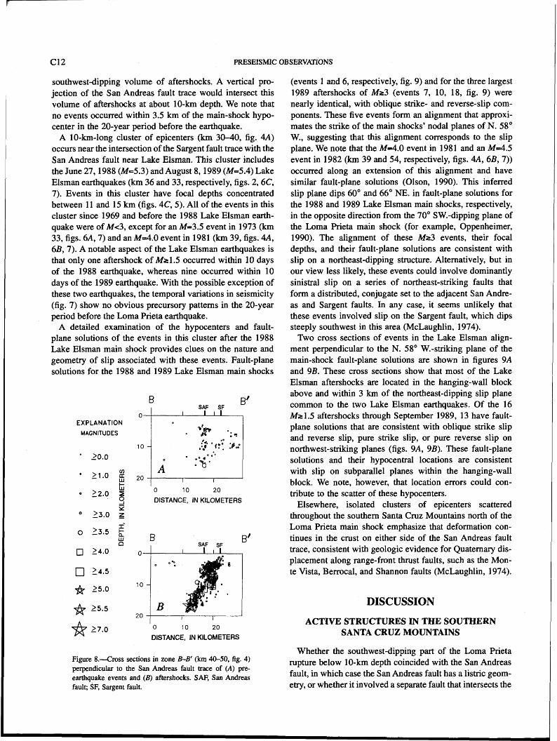
A 10-km-long cluster of epicenters (krn 30-40, fig. 4A) occurs near the intersection of the Sargent fault trace with the San Andreas fault near Lake Elsman. This cluster includes the June 27,1988 (M=5.3) and August 8,1989 (M=5.4) Lake Elsman earthquakes (krn 36 and 33, respectively, figs. 2,6C, 7). Events in this cluster have focal depths concentrated between 11 and 15 km (figs. 4C, 5). All of the events in this cluster since 1969 and before the 1988 Lake Elsman earth- quake were of Mc3, except for an M=3.5 event in 1973 (km 33, figs. 6A, 7) and an M=4.0 event in 1981 (krn 39, figs. 4A, 6B, 7). A notable aspect of the Lake Elsman earthquakes is that only one aftershock of Ms1.5 occurred within 10 days of the 1988 earthquake, whereas nine occurred within 10 days of the 1989 earthquake. With the possible exception of these two earthquakes, the temporal variations in seismicity (fig. 7) show no obvious precursory patterns in the 20-year period before the Loma Prieta earthquake.
A detailed examination of the hypocenters and fault- plane solutions of the events in this cluster after the 1988 Lake Elsman main shock provides clues on the nature and geometry of slip associated with these events. Fault-plane solutions for the 1988 and 1989 Lake Elsman main shocks
EXPLANATION MAGNITUDES
0 10 20
DISTANCE. IN KILOMETERS
0 10 20
DISTANCE. IN KILOMETERS
Figure 8.ÑCros sections in zone B-B' (km 40-50, fig. 4) perpendicular to the San Andreas fault trace of (A) pre- earthquake events and (B) aftershocks. SAP, San Andreas fault; SF, Sargent fault.
(events 1 and 6, respectively, fig. 9) and for the three largest 1989 aftershocks of M23 (events 7, 10, 18, fig. 9) were nearly identical, with oblique strike- and reverse-slip com- ponents. These five events form an alignment that approxi- mates the strike of the main shocks* nodal planes of N. 58' W., suggesting that this alignment corresponds to the slip plane. We note that the M=4.0 event in 1981 and an M=4.5 event in 1982 (km 39 and 54, respectively, figs. 4A, 6B, 7)) occurred along an extension of this alignment and have similar fault-plane solutions (Olson, 1990). This inferred slip plane dips 60' and 66' NE. in fault-plane solutions for the 1988 and 1989 Lake Elsman main shocks, respectively, in the opposite direction from the 70Â SW.-dipping plane of the Loma Prieta main shock (for example, Oppenheimer, 1990). The alignment of these M23 events, their focal depths, and their fault-plane solutions are consistent with slip on a northeast-dipping structure. Alternatively, but in our view less likely, these events could involve dominantly sinistral slip on a series of northeast-striking faults that form a distributed, conjugate set to the adjacent San Andre- as and Sargent faults. In any case, it seems unlikely that these events involved slip on the Sargent fault, which dips steeply southwest in this area (McLaughlin, 1974).
Two cross sections of events in the Lake Elsman align- ment perpendicular to the N. 58' W.-striking plane of the main-shock fault-plane solutions are shown in figures 9A and 9B. These cross sections show that most of the Lake Elsman aftershocks are located in the hanging-wall block above and within 3 km of the northeast-dipping slip plane common to the two Lake Elsman earthquakes. Of the 16 Ms 1.5 aftershocks through September 1989, 13 have fault- plane solutions that are consistent with oblique strike slip and reverse slip, pure strike slip, or pure reverse slip on northwest-striking planes (figs. 9A, 95). These fault-plane solutions and their hypocentral locations are consistent with slip on subparallel planes within the hanging-wall block. We note, however, that location errors could con- tribute to the scatter of these hypocenters.
Elsewhere, isolated clusters of epicenters scattered throughout the southern Santa Cruz Mountains north of the Loma Prieta main shock emphasize that deformation con- tinues in the crust on either side of the San Andreas fault trace, consistent with geologic evidence for Quaternary dis- placement along range-front thrust faults, such as the Mon- te Vista, Berrocal, and Shannon faults (McLaughlin, 1974).
DISCUSSION
ACTIVE STRUCTURES IN THE SOUTHERN SANTA CRUZ MOUNTAINS
Whether the southwest-dipping part of the Loma Prieta rupture below 10-km depth coincided with the San Andreas fault, in which case the San Andreas fault has a listric geom- etry, or whether it involved a separate fault that intersects the

SEISMICITY IN THE SOUTHERN SANTA CRUZ MOUNTAINS DURING THE 20-YEAR PERIOD BEFORE THE EARTHQUAKE C 13
NATION MAGNITUDE!
OF FAULT PLANE SOLUTIONS
0 21.5
0 22.0
0 3 . 0
0 3 . 5
0 24.0
0 24.5
0 25.0
EXPL - MAGNITUDE
OF EPICENTER!
AND HYPOCENTEF
. 20.0
21.0
22.0
23.0
0 23.5
-J 24.0
J 24.5
25.0
dip
-r----- KILOMETERS - 0 1 2 3 4 5 DISTANCE, IN KILOMETERS
in' .- /\ \ / -
b 122O15' 37O 122O 1 21Â 45' 36" 45'
4)
CM5.41 \ 7 9 KILOMETERS I I
0 1 2 I
[J
0 1 2 3 4 5 DISTANCE, IN KILOMETERS
Figure 9.-Lake Elsman area (inset), showing locations of epicenters and fault-plane solutions (for Mz1.5 events) and cross sections for earthquakes between (A) time of June 27, 1988 (G.m.t.), Lake Elsman (M=5.3) main shock up to time of August 8,1989 (G.m.t.), Lake Elsman main shock and (B) time of 1989 Lake Elsman main shock up to time of Loma Prieta main shock (fault-plane solutions are shown only for events through September). Hypocenters in cross sections are projected onto a plane through line C-C' that is perpendicular to main shocks' nodal planes striking N. 58' W., and
those nodal planes' dips of 60' and 66' NE. are shown, projected through each main-shock hypocenter. C, First-motion data for fault-plane solutions shown in figures 9A and 95, with corresponding numbers. Plusses, com- pressional first motion; circles, dilatational first motion; P, principal axis of compression; T, principal axis of extension. Headings list yearlmonthlday and hourlminute (G.m.t.); M, magnitude (see text); Z, depth (in kilometers). Fault lines: solid, well located; dashed, approximately located or inferred; dotted, concealed by younger rocks or by lakes or bays.

C14 PRESEISMIC OBSERVATIONS
San Andreas fault at about 10-km depth remains a matter of discussion (Dietz and Ellsworth, 1990; Olson, 1990). The few events between 10- and 16-km depth directly beneath the San Andreas fault trace and east of the main-shock hypo- center could be produced by either (1) the San Andreas fault, in which case the Loma Prieta rupture below 10-km depth involved a separate fault; or (2) discontinuous faults to the east of a southwest-dipping San Andreas fault, as Ellsworth and others (1990) suggested. In either case, several adjacent faults in the southern Santa Cruz Mountains clearly accom- modate both strike-slip motion and a small component of
crustal convergence. This complex system of interacting faults reflects a combination of the broad restraining bend that the San Andreas fault forms in the study area, the triple junction formed by the intersection of the San Andreas and Calaveras faults to the south, and regional transpression common to the entire San Francisco Bay region (Aydin and Page, 1984; Harbert and Cox, 1989; Harbert, 1991).
One notable aspect of both the preearthquake and after- shock hypocenters is the broad, U-shaped distribution de- fined by the deepest events in both time periods that spans a zone at least 10 krn wide. This depth distribution, which was first noted by Moths and others (1981) and Lindh and others (1982) for seismicity between 1969 and 1981, was one line of evidence they used to suggest that the southern Santa Cruz Mountains section of the San Andreas fault zone was likely to produce a large earthquake. Relative locations of preearthquake events and aftershocks in our study, however, show that the preearthquake events forrn- ing this U-shaped depth distribution are located northeast of the principal, southwest-dipping section of the Loma Prieta aftershock zone below about 10-km depth. Thus, this depth distribution is apparently related to crustal properties that span the 10-km width of the fault zone, rather than to prop- erties limited to a particular fault plane. For example, max- imum earthquake focal depths along the strike of the fault zone may be related in some way to the relatively high P- wave velocities calculated across the zone in three-dimen- sional velocity models (Eberhart-Phillips and others, 1990; Lees, 1990; Foxall and others, 1991). Foxall and others (1991) interpreted these high-velocity rocks as either up- thrusted gneissic or ultramafic subcrustal rocks.
PREVIOUS Ma:5 EARTHQUAKES ALONG THE LOMA PRIETA RUPTURE ZONE
The Lake Elsman earthquakes stand out against the back- ground seismicity for the 20-year period before the Loma Prieta earthquake because they are the only Ms5 earth- quakes along the rupture zone in that period and they oc- curred within 16 and 2% months beforehand (see fig. 7). They also are unusual because they are a full unit of mag- nitude larger than the preceding events in this spatial clus- ter within this time period. An examination of the catalogs by Bolt and Miller (1975) and Toppozada and others (1978) reveals that only one documented M25.0 event since 1910 occurred within a 15-km radius of the 1988 and 1989 Lake Elsman earthquakes: an M,=5.5 earthquake on November 9, 1914 (see fig. 2), as described Townley and Allen (1939):
VIII. Santa Cruz Mountains. From reports received and from field inves- tigations, Carl H. Beal determined the epicenter of this earthquake to have been near the small town of Laurel, Santa Cruz Co., near the crest of the Santa Cruz Mountains and about seven miles south of Los Gatos. Laurel is a mile southwest of the San Andreas fault. At Laurel two chim- neys were broken off, clocks were stopped, and plaster cracked * * *. The shock was felt * * * at distances of about 100 miles, indicating a shaken area of approximately 30,000 square miles. Figure 9.ÑContinued

SEISMICITY IN THE SOUTHERN SANTA CRUZ MOUNTAINS DURING THE 20-YEAR PERIOD BEFORE THE EARTHQUAKE C 15
Although this event may be considered an aftershock of the 1906 earthquake and evidently produced the highest intensi- ties near the San Andreas fault near Laurel, it need not have occurred on the San Andreas fault itself. It could, for exam- ple, have occurred on the same structure that produced the Lake Elsman earthquakes. Thus, the record of moderate earthquakes since 1910 indicates that the structure that pro- duced the Lake Elsman earthquakes had not produced Mz5.0 events since at least 1914, or within the past 74 years.
Five other Mz5 earthquakes since 1910 may also have occurred along the Loma Prieta rupture zone, east and southeast of the main shock. Only two of these earth- quakes, however, have epicenters located well enough to be associated with that zone to some degree of certainty (with- in -10 km): the 1964 (M=5.0) and 1967 (M=5.3) Corralitos earthquakes. A relocation of the 1964 earthquake (McEvil- ly, 1966) suggests that it was associated with the same structure which produces seismicity along and northeast of the south end of the Sargent fault. The 1967 epicenter, how- ever, is apparently located farther to the southwest and closer to the San Andreas fault trace. Thus, four moderate (M=5) earthquakes apparently occurred along the Loma Prieta rupture zone within the preceding 25 years.
SUMMARY
1. Well-located earthquakes in the study area since 1969 and before the Loma Prieta earthquake define conspicu- ous alignments along the creeping section of the San Andreas fault south of Pajaro Gap, along and east of the Sargent fault, and along the Busch Ranch and Calaveras faults. In addition, a cluster of events occurred along and east of a 10-krn-long section of the Sargent fault where it intersects the San Andreas fault. The events along and east of the Sargent fault apparently are not associated with that fault, which dips steeply southwest. The events near the north end of the Sargent fault include the 1988 (M=5.3) and the 1989 (M=5.4) Lake Elsman earth- quakes, located 10 and 12 km, respectively, north-north- east of the Loma Prieta main shock. Elsewhere, a few events occurred along the 35-km-long section of the San Andreas fault trace between Pajaro Gap and Lake Els- man, and isolated events occurred on both sides of the San Andreas fault trace throughout the southern Santa Cruz Mountains north of the Loma Prieta main shock.
2. Fault-plane solutions for both the 1988 and 1989 Lake Elsman main shocks show oblique strike slip and reverse slip on a plane that strikes N. 58' W. and dips 60'-66' NE., suggesting that these earthquakes may have oc- curred on a common, blind fault. Fault-plane solutions and hypocenters for most of the Lake Elsman aftershocks (Ms1.5) are consistent with oblique slip in the hanging- wall block on planes subparallel to the inferred slip plane common to the 1988 and 1989 Lake Elsman main shocks.
3. The Lake Elsman earthquakes are unusual even though they occurred within an area of persistent background
seismicity, because they were a full unit of magnitude larger than all other events recorded within a 15-km ra- dius during the preceding 74 years, because they are the only Mz5 events in the 20-year period before the Loma Prieta earthquake located along the rupture zone, and because they occurred within 16 and 2% months before- hand. Two other M25 earthquakes since 1960, however, also occurred along the rupture zone: the 1964 (M=5.0) and 1967 (M=5.3) Corralitos earthquakes, located ap- proximately 17 km east and 10 km southeast, respec- tively, of the Loma Prieta main shock. Given location errors greater than 10 km for earthquakes before 1960 in the southern Santa Cruz Mountains, other M25 events may have occurred along the rupture zone since 1910, including those in 1910 (M=5.5), 1914 (M=5.5), 1954 (Mz5.3) and 1959 (M=5.3).
4. The southwest-dipping section of the Loma Prieta rup- ture zone beneath 10-km depth produced virtually no microseismicity for at least 20 years before the Loma Prieta earthquake.
5. The hypocenters of earthquakes occurring in the study area since 1969 form a broad U-shaped distribution when projected onto a vertical plane parallel to the San Andre- as fault trace. This depth distribution of preearthquake seismicity approximately forms a lower bound to the dis- tribution of Loma Prieta aftershocks, even though the events below 10-km depth both before and after the earthquake occurred on different fault planes within the 10-km-wide zone.
ACKNOWLEDGMENTS
We thank J.P. Eaton, W.L. Ellsworth, A.G. Lindh, D.H. Oppenheimer, and P.A. Reasenberg for their helpful re- views of the manuscript, and F.W. Klein and D.H. Oppen- heimer for providing Calnet-catalog data.
REFERENCES CITED Anderson, R.S., 1990, Evolution of the northern Santa Cruz Mountains
by advection of crust past a San Andreas fault bend: Science, v. 249, no. 4967, p. 397-401.
Aydin, Atilla, and Page, B.M., 1984, Diverse Pliocene-Quaternary tectonics in a transform environment, San Francisco Bay region, California: Geological Society of America Bulletin, v. 95, no. 11, p. 1303-1317.
Beroza, G.C., 1991, Near-source modeling of the Loma Prieta earth- quake; evidence for hererogeneous slip and implications for earth- quake hazard: Seismological Society of America Bulletin, v. 81, no. 5, p. 1603-1621,
Bolt, B.A., and Miller, R.D., 1975, Catalog of earthquakes in northern California and adjoining areas, 1 January 1930-31 December 1972: Berkeley, University of California, Seismographic Station, 567 p.
Burford, R.O., and Harsh, P.W., 1980, Slip on the San Andreas fault in central California from alinement array surveys: Seismological So- ciety of America Bulletin, v. 70, no. 4, p. 1233-1261.
Dietz, L.D., and Ellsworth, W.L., 1990, The October 17, 1989 Loma Pri- eta, California, earthquake and its aftershocks; geometry of the se- quence from high-resolution locations: Geophysical Research Letters, v. 17, no. 9, p. 1417-1420.

C16 PRESEISMIC OBSERVATIONS
Eaton, J.P., 1989, Dense microearthquake network study of northern Cal- ifornia earthquakes, chap. 13 of Litehiser, J.J., ed., Observatory seis- mology, a centennial symposium for the Berkeley Seismographic Stations: Berkeley, University of California Press, p. 199-224.
1992, Determination of amplitude and duration magnitudes and site residuals from short-period seismographs in northern California: Seismological Society of America Bulletin, v. 82, no. 2, p. 533-579.
Eaton, J.P., Lee, W.H.K., and Pakiser, L.C., 1970, Use of microearth- quakes in the study of the mechanics of earthquake generation along the San Andreas fault in central California: Tectonophysics, v. 9, no. 2-3, p. 259-282.
Eberhart-Phillips, Donna, Labson, V.F., Stanley, W.D., Michael, A.J., and Rodriguez, B.D., 1990, Preliminary velocity and resistivity models of the Loma Prieta earthquake region: Geophysical Research Let- ters, v. 17, no. 8, p. 1235-1238.
Ellsworth, W.L., 1990, Earthquake history, 1769-1989, chap. 6 of Wal- lace, R.E., ed., The San Andreas fault system, California: U.S. Geo- logical Survey Professional Paper 1515, p. 153-188.
Ellsworth, W.L., Dietz, L.D., and Lindh, A.G., 1990, Accommodation of North America-Pacific plate motion along the Loma Prieta earth- quake rupture zone; where is the real San Andreas fault? [abs.]: Eos (American Geophysical Union Transactions), v. 71, no. 43, p. 1646.
Foxall, William, Michelini, Alberto, and McEvilly, T.V., 1991, Structure and fault processes of the Loma Prieta earthquake from a three- dimensional P-velocity model [abs.]: Eos (American Geophysical Union Transactions), v. 72, no. 44, supp., p. 3 11.
Harbert, William, 1991, Late Neogene relative motions of the Pacific and North American Plates: Tectonics, v. 10, no. 1, p. 1-15.
Harbert, William, and Cox, Allan, 1989, Late Neogene motion of the Pacific Plate: Journal of Geophysical Research, v. 94, no. B3, p. 3052-3064.
Hill, D.P., Eaton, J.P., and Jones, L.M, 1990, Seismicity, 1980-86, chap. 5 of Wallace, R.E., ed.. The San Andreas fault system, California: U.S. Geological Survey Professional Paper 15 15, p. 1 15-1 52.
Hill, D.P., Eaton, J.E., Ellsworth, W.L., Cockerham, R.S., Lester, F.W., and Corbett, E.J., 1991, The seismotectonic fabric of central Cali- fornia, in Slemmons, D.B., Engdahl, E.R., Blackwell, D.D., Schwartz, D.P., and Zoback, M.D., eds., Neotectonics of North America (DNAG Associated Volume GSMV-1): Boulder, Colo., Geological Society of America, p. 107-132.
Irwin, W.P., 1990, Geology and plate-tectonic development, chap. 3 of Wallace, R.E., ed., The San Andreas fault system, California: U.S. Geological Survey Professional Paper 15 15, p. 6 1-82.
King, G.C.P, Lindh, A.G., and Oppenheimer, D.H., 1990, Seismic slip, segmentation, and the Loma Prieta earthquake: Geophysical Re- search Letters, v. 17, no. 9, p. 1449-1452.
Klein, F.W., 1989, User's guide to HYPOINVERSE, a program for VAX computers to solve earthquake locations and magnitudes: U.S. Geo- logical Survey Open-File Report 89-314.58 p.
Lee, W.H.K., and Stewart, S.W., 1981, Principles and applications of mi- croearthquake networks: New York, Academic Press, 293 p.
Lees, J.M., 1990, Tomographic P-wave velocity images of the Loma Pri- eta earthquake asperity: Geophysical Research Letters, v. 17, no. 9, p. 1433-1436.
Lindh, A.G., Moths, B.L., Ellsworth, W.L., and Olson, J.A., 1982, His- toric seismicity of the San Juan Bautista, California region [abs.], in Hill, D.P., and Nishimura, Keiji, chairmen, U.S.-Japan Conference on Natural Resources (UJNR), Panel on Earthquake Prediction Technology Joint Meeting, 2d, Men10 Park, Calif., 198 1, Proceed- ings: U.S. Geological Survey Open-File Report 82-180, p. 45-50.
Lisowski, Michael, Prescott, W.H., Savage, J.C., and Johnston, M.J.S., 1990, Geodetic estimates of coseismic slip during the 1989 Loma Prieta, California earthquake: Geophysical Research Letters, v. 17, no. 9, p. 1437-1440.
McEvilly, T.V., 1966, The earthquake sequence of November 1964 near Corralitos, California: Seismological Society of America Bulletin, v. 56, no. 3, p. 755-773.
McLaughlin, R.J., 1974, The Sargent-Berrocal fault zone and its relation to the San Andreas fault system in the southern San Francisco Bay region and Santa Clara Valley, California: U.S. Geological Survey Journal of Research, v. 2, no. 5, p. 593-598.
Moths, B.L., Lindh, A.G., Ellsworth, W.L., and Fluty, L., 1981, Compari- son between the seismicity of the San Juan Bautista and Parkfield regions, California [abs.]: Eos (American Geophysical Union Trans- actions), v. 62, p. 958.
Olson, J.A., 1990, Seismicity in the twenty years preceding the 1989 Loma Prieta, California earthquake: Geophysical Research Letters, v. 17, no 9, p. 1429-1432.
Oppenheimer, D.H., 1990, Aftershock slip behavior of the 1989 Loma Prieta, California earthquake: Geophysical Research Letters, v. 17, no. 8, p. 1199-1202.
Pavoni, N., 1973, A structural model for the San Andreas fault zone along the northeast side of the Gablilan Range, in Kovach, R.L., and Nur, Amos, eds., Proceedings of the conference on tectonic problems of the San Andreas fault system: Stanford, Calif., Stanford University Publications in the Geological Sciences, v. 13, p. 259- 267.
Reasenberg, Paul, and Oppenheimer, D.H., 1985, FPFIT, FPPLOT, and FPPAGE, FORTRAN computer programs for calculating and dis- playing earthquake fault-plane solutions: U.S. Geological Survey Open-File Report 85-739, 109 p.
Rogers, T.H., 1980, Geology and seismicity at the convergence of the San Andreas and Calaveras fault zones near Hollister, San Benito County, California, in Streitz, Robert, and Sherburne, R.W., eds., Studies of the San Andreas fault zone in northern California: Cali- fornia Division of Mines and Geology Special Report 140, p. 19- 28.
Schulz, S.S., Mavko, G.M., Burford, R.O., and Stuart, W.D., 1982, Long- term fault creep observations in central California: Journal of Geo- physical Research, v. 87, no. B8, p. 6977-6982.
Seeber, Leonardo, and Arrnbruster, J.G., 1990, Fault kinematics in the 1989 Loma Prieta rupture area during 20 years before that event: Geophysical Research Letters, v. 17, no. 9, p. 1425-1428.
Segall, Paul, and Lisowski, Michael, 1990, Surface displacements in the 1906 San Francisco and 1989 Loma Prieta earthquakes: Science, v. 250, no. 4985, p. 1241-1244.
Spieth, M.A., 1981, Two detailed seismic studies in central California. Part I: Earthquake clustering and crustal structure studies of the San Andreas fault near San Juan Bautista. Part 11: Seismic velocity structure along the Sierra foothills near Oroville, California: Stan- ford, Calif., Stanford University, Ph.D. thesis, 174 p.
Steidl, J.H., Archuleta, R.J., and Hartzell, S.H., 1991, Rupture history of the 1989 Loma Prieta, California earthquake: Seismological Society of America Bulletin, v. 81, no. 5, p. 1573-1602.
Thatcher, Wayne, 1990, Present-day crustal movements and the mechan- ics of cyclic deformation, chap. 7 of Wallace, R.E., ed., The San Andreas fault system, California: U.S. Geological Survey Profes- sional Paper 1515, p. 153-188.
Toppozada, T.R., Parke, D.L., and Higgins, C.T., 1978, Seismicity of California, 1900-193 1: California Division of Mines and Geology Special Report 135,39 p.
Townley, S.D., and Allen, M.W., 1939, Descriptive catalog of earth- quakes of the Pacific coast of the United States, 1769 to 1928: Seis- mological Society of America Bulletin, v. 29, no. 1, p. 1-297.
Valensise, Gianluca, and Ward, S.N., 1991, Long-term uplift of the Santa Cruz coastline in response to repeated earthquakes along the San Andreas fault: Seismological Society of America Bulletin, v. 81, no. 5, p. 1694-1704.
Wald, D. J., Helmberger, D.V., and Heaton, T.H., 1991, Rupture model of the 1989 Loma Prieta earthquake from the inversion of strong mo- tions and broadband teleseismic data: Seismological Society of America Bulletin, v. 81, no. 5, p. 1540-1572.

THE LOMA PRIETA, CALIFORNIA, EARTHQUAKE OF OCTOBER 17,1989: EARTHQUAKEOCCURRENCE
PRESEISMIC OBSERVATIONS
ANALYSIS OF LOW-FREQUENCY-ELECTROMAGNETIC-FIELD MEASUREMENTS NEAR THE EPICENTER
By Anthony C. Fraser-Smith, Arman Bernardi,' Robert A. Helliwell, Paul R. McGill, and O.G. Villard, Jr., Stanford University
CONTENTS
ABSTRACT
We summarize the results of measurements of low-fre- quency electromagnetic fields by two independent moni- toring systems before the earthquake. Taken together, these measurements cover 25 narrow frequency bands in the more than six-decade frequency range 0.01 Hz-32 kHz, with a time resolution ranging from half an hour in the ultra-low-frequency (ULF) range (0.01-10 Hz) to 1 s in the extremely low frequencylvery low frequency (ELF1 VLF) range (10 Hz-32 kHz). The ULF system is located near Corralitos, Calif., about 7 km from the epicenter, and the ELFNLF system on the Stanford University campus, about 52 km from the epicenter. As previously reported, analysis of these ELFNLF data has revealed no precurso- ry activity, although the ULF data have some distinctive and anomalous features. First, a narrow-band signal in the range 0.05-0.2 Hz appeared about September 12 and per- sisted until the appearance of a second anomalous feature, which consisted of a substantial increase in the noise background starting on October 5 that covered almost the entire frequency range of the ULF system but was greatest at the lowest frequencies. Third, there was an anomalous dip in the noise background in the range 0.2-5 Hz starting 1 day before the earthquake. Finally and, possibly, most
current affiliation: Teknekron Communications Systems, Berkeley, CA 94704.
compelling, there was an increase to an exceptionally high level of activity in the range 0.01-0.5 Hz (that is, at the lowest frequencies) starting approximately 3 hours before the earthquake. There do not appear to have been any mag- netic-field fluctuations originating in the upper atmosphere that can account for this increase. Furthermore, although the measurement systems are sensitive to motion, seismic measurements indicate no significant shocks before the earthquake. Thus, the various anomalous features in the da- ta, particularly the large-amplitude increase in activity starting 3 hours before the earthquake, may have been magnetic precursors. The observation of the largest mag- netic-field amplitudes at the lowest frequencies, and the ab- sence of ELFNLF signals, suggest that the anomalous signals may have originated in the hypocentral region and propagated to the surface. If so, modeling with electric- and magnetic-dipole sources further suggests that the ULF signals could have been detected at the surface as far as 100 km from the epicenter.
INTRODUCTION
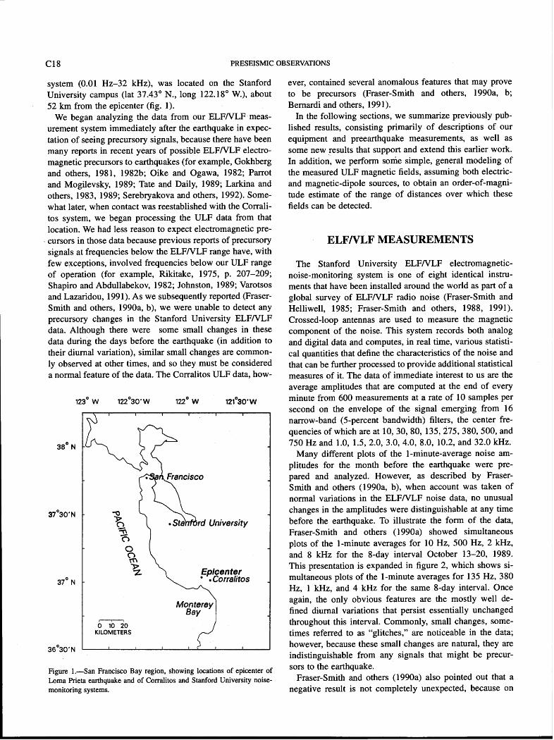
At 5:04 p.m. P.d.t. October 17, 1989 (0004:15.24 G.m.t. Oct. 1 8), a moderately large (Me =7.1) earthquake occurred "suddenly and without foreshock activity" in northern Cali- fornia (U.S. Geological Survey staff, 1990). Its epicenter (lat 37.039' N., long 121.879' W.) was located near Loma Prieta, one of the highest peaks in the California Coast Ranges, just south of the San Francisco Bay region (fig. 1). At the time of the earthquake, we were operating two inde- pendent electromagnetic-noise-monitoring systems at loca- tions relatively close to the epicenter, in continuation of a program of low-frequency-radio-noise measurements that has been in progress for several years. Taken together, these two systems provided complete coverage of magnet- ic-field changes over the broad frequency range from 0.01 Hz to 32 kHz. One, an ultra-low-frequency (ULF) system (0.01-10 Hz), was located at Corralitos, Calif. (lat 37.015' N., long 121.806' W.), only 7 km from the epicenter; and the other, an extremely lowlvery low frequency (ELFNLF)
C18 PRESEISMIC OBSERVATIONS
system (0.01 Hz-32 kHz), was located on the Stanford University campus (lat 37.43' N., long 122.18' W.), about 52 km from the epicenter (fig. 1).
We began analyzing the data from our ELFNLF meas- urement system immediately after the earthquake in expec- tation of seeing precursory signals, because there have been many reports in recent years of possible ELFNLF electro- magnetic precursors to earthquakes (for example, Gokhberg and others, 1981, 1982b; Oike and Ogawa, 1982; Parrot and Mogilevsky, 1989; Tate and Daily, 1989; Larkina and others, 1983, 1989; Serebryakova and others, 1992). Some- what later, when contact was reestablished with the Corrali- tos system, we began processing the ULF data from that location. We had less reason to expect electromagnetic pre- cursors in those data because previous reports of precursory signals at frequencies below the ELFNLF range have, with few exceptions, involved frequencies below our ULF range of operation (for example, Rikitake, 1975, p. 207-209; Shapiro and Abdullabekov, 1982; Johnston, 1989; Varotsos and Lazaridou, 1991). As we subsequently reported (Fraser- Smith and others, 1990a, b), we were unable to detect any precursory changes in the Stanford University ELFNLF data. Although there were some small changes in these data during the days before the earthquake (in addition to their diurnal variation), similar small changes are cornrnon- ly observed at other times, and so they must be considered a normal feature of the data. The Corralitos ULF data, how-
Monterey - 0 10 20
KILOMETERS
Figure 1.-San Francisco Bay region, showing locations of epicenter of Loma Prieta earthquake and of Corralitos and Stanford University noise- monitoring systems.
ever, contained several anomalous features that may prove to be precursors (Fraser-Smith and others, 1990a, b; Bernardi and others, 1991).
In the following sections, we summarize previously pub- lished results, consisting primarily of descriptions of our equipment and preearthquake measurements, as well as some new results that support and extend this earlier work. In addition, we perform some simple, general modeling of the measured ULF magnetic fields, assuming both electric- and magnetic-dipole sources, to obtain an order-of-magni- tude estimate of the range of distances over which these fields can be detected.
ELF/VLF MEASUREMENTS
The Stanford University ELFNLF electromagnetic- noise-monitoring system is one of eight identical instru- ments that have been installed around the world as part of a global survey of ELFNLF radio noise (Fraser-Smith and Helliwell, 1985; Fraser-Smith and others, 1988, 1991). Crossed-loop antennas are used to measure the magnetic component of the noise. This system records both analog and digital data and computes, in real time, various statisti- cal quantities that define the characteristics of the noise and that can be further processed to provide additional statistical measures of it. The data of immediate interest to us are the average amplitudes that are computed at the end of every minute from 600 measurements at a rate of 10 samples per second on the envelope of the signal emerging from 16 narrow-band (5-percent bandwidth) filters, the center fre- quencies of which are at 10, 30, 80, 135, 275, 380, 500, and 750 Hz and 1.0, 1.5, 2.0, 3.0, 4.0, 8.0, 10.2, and 32.0 kHz.
Many different plots of the 1-minute-average noise am- plitudes for the month before the earthquake were pre- pared and analyzed. However, as described by Fraser- Smith and others (1990a, b), when account was taken of normal variations in the ELFNLF noise data, no unusual changes in the amplitudes were distinguishable at any time before the earthquake. To illustrate the form of the data, Fraser-Smith and others (1990a) showed simultaneous plots of the 1-minute averages for 10 Hz, 500 Hz, 2 kHz, and 8 kHz for the 8-day interval October 13-20, 1989. This presentation is expanded in figure 2, which shows si- multaneous plots of the 1-minute averages for 135 Hz, 380 Hz, 1 kHz, and 4 kHz for the same 8-day interval. Once again, the only obvious features are the mostly well de- fined diurnal variations that persist essentially unchanged throughout this interval. Commonly, small changes, some- times referred to as "glitches," are noticeable in the data; however, because these small changes are natural, they are indistinguishable from any signals that might be precur- sors to the earthquake.
Fraser-Smith and others (1990a) also pointed out that a negative result is not completely unexpected, because on

ANALYSIS OF LOW-FREQUENCY-ELECTROMAGNETIC-FIELD MEASUREMENTS NEAR THE EPICENTER C19
three earlier occasions unsuccessful searches had been made for precursory signals in the Stanford University ELFIVLF noise data after local earthquakes of M-5 (Alum Rock, June 13, 1988, ML=5.3; Lake Ellsman 1, June 27, 1988, ML=5.0; Lake Ellsman 2, August 8, 1989, ML=5.2). Since the publication of these negative results, an exten- sive search has also been made for precursory signals in the ELFNLF wave data obtained by the low-altitude Dy- namics Explorer 2 (DE-2) satellite (apogee, -1,300 km; perigee, -300 km; inclination, -90') near the times of 60 earthquakes, but without success (Henderson and others, 1991). The results of these various studies show that measurable ELFNLF electromagnetic precursors are not always associated with earthquakes.
ULF MEASUREMENTS
The Corralitos magnetic-field-monitoring system is one of four new models that we have built to characterize and monitor the state of natural geomagnetic activity in the ULF range 0.01-10 Hz (Bernardi and others, 1989). They are conventional in many of their technical details, includ- ing their use of solenoidal coils as sensors; however, they differ significantly from previous systems used by our lab- oratory and others for measurements of ULF geomagnetic- field changes, through their use of a small computer as an integral part of the measurement system and through an emphasis on the real-time computation of digital measure- ments of the noise power as an alternative to analog chart
DATE (OCTOBER 1989)
Figure 2.-1-minute-average extremely low frequencylvery low frequency noise amplitudes measured during interval October 13-20, 1989, at Stanford University for frequencies of (A) 135 Hz, (B) 380 Hz, (0 1 kHz, and (D) 4 kHz. Earthquake occurred just after 0004 G.m.t. October 18 (arrow), followed immediately by an 8-hour power failure. Large transient impulses during 1-hour period immediately after recommencement of measurements are probably related to automatic restart, instead of aftershock activity. Note different ampli- tude scales.
c20 PRESEISMIC OBSERVATIONS
Table 1.-Frequency ranges for which magnet- ic-activity (MA) indices are computed, and their center frequencies
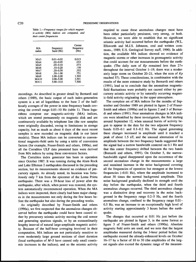
MA index
Center frequency frequency band (Hz) (Hz)
recordings. As described in greater detail by Bernardi and others (1989), the basic output of each index-generation system is a set of logarithms to the base 2 of the half- hourly averages of the power in nine frequency bands cov- ering the overall range 0.01-10 Hz (table 1). These loga- rithms compose our magnetic-activity (MA) indices, which are stored permanently on magnetic disk and are continuously available by telephone line (the raw samples were originally discarded, owing to limitations in storage capacity, but as much as about 6 days of the most recent samples is now recorded on magnetic disk in our latest models). These MA indices can be converted to conven- tional magnetic-field units by using a table of conversion factors (for example, Fraser-Smith and others, 1990a), and all the Corralitos ULF data presented here were derived from MA indices by using these conversion factors.
The Corralitos index generator has been in operation since October 1987. It was running during the Alum Rock and Lake Ellsman 2 earthquakes discussed in the preceding section, but its measurements showed no evidence of pre- cursory signals. As already noted, its location was fortu- itously only 7 km from the epicenter of the Loma Prieta earthquake. There was a 39-hour loss of power after the earthquake, after which, when power was restored, the sys- tem automatically recommenced operation. When the MA indices were inspected, there clearly had been major chang- es in the measurements not only during the few hours be- fore the earthquake but also during the preceding weeks.
As originally described by Fraser-Smith and others (1990a), we first suspected that the anomalous changes ob- served before the earthquake could have been caused ei- ther by precursory seismic activity moving the coil sensor and generating spurious signals, or by an extraordinarily lengthy interval of natural large-amplitude magnetic activi- ty. Because of the half-hour averaging involved in their computation, MA indices are not particularly sensitive to even moderately large ground motions of short duration (local earthquakes of M-5 have caused only small coseis- mic increases in the indices), and so the seismic activity
required to cause these anomalous changes must have been either particularly persistent, very strong, or both. However, we were able to establish that no significant seismic activity had occurred before the earthquake (W.L. Ellsworth and M.J.S. Johnston, oral and written com- muns., 1989; U.S. Geological Survey staff, 1990). In addi- tion, the available MA indices showed no evidence of magnetic storms or other increases in geomagnetic activity that could account for our measurements before the earth- quake. (The daily sum of Kp remained less than 27+ throughout the interval October 1-19; there was a moder- ately large storm on October 20-21, when the sum of Kp reached 57). These considerations, in combination with the results of the more extensive study by Bernardi and others (1991), lead us to conclude that the anomalous magnetic- field fluctuations were probably not caused either by pre- cursory seismic activity or by naturally occurring magnet- ic-field activity originating in the upper atmosphere.
The complete set of MA indices for the months of Sep- tember and October 1989 are plotted in figure 2 of Fraser- Smith and others (1990a) and in figures 2 and 3 of Bernar- di and others (1991). Four anomalous changes in MA indi- ces were identified by these investigators, the first starting around September 12, when unusual bursts of activity be- gan to appear in the data for the two adjacent frequency bands 0.05-0.1 and 0.1-0.2 Hz. The signal generating these changes increased in amplitude until it reached a peak of about 1.5 nT, and the unusual alternation of its amplitude between the two frequency bands suggested that the signal had a narrow bandwidth centered on 0.1 Hz and that this center frequency drifted between the two bands (Bernard! and others, 1991). On October 5, the narrow- bandwidth signal disappeared upon the occurrence of the second anomalous change in the measurements: a large and sustained increase in the noise background covering all the frequencies of operation but strongest at the lowest frequencies ( 4 . 01 Hz), where the amplitude increased to about 30 times the normal background amplitude. This noise background gradually declined in strength until the day before the earthquake, when the third and fourth anomalous changes occurred. The third anomalous change was a distinctive drop and recovery in the noise back- ground in the frequency range 0.2-5 Hz, and the fourth anomalous change, confined to the frequency range 0.01- 0.5 Hz, was an increase to an exceptionally high level of activity starting approximately 3 hours before the earth- quake.
The changes that occurred at 0.01 Hz just before the earthquake are plotted in figure 3, in the same format as figure 3 of Fraser-Smith and others (1990a). Absolute magnetic field units are used, and we note that the largest amplitudes measured during the 3-hour period before the earthquake exceed the already-enhanced levels on October 16-17 by a factor of 10 to 30 (the amplitudes of the larg- est signals also exceed the dynamic range of the measure-

ANALYSIS OF LOW-FREQUENCY-ELECTROMAGNETIC-FffiLD MEASUREMENTS NEAR THE EPICENTER C21
ment system, and so the measured amplitudes are actually smaller than the true values). The data obtained during the aftershock interval, some of which are plotted in figure 3, are of great interest, but their analysis is made difficult by the large number and variety of aftershocks, by the shak- ing response of the measurement system, and by the oc- currence of a magnetic storm on October 20-21. Analysis of these aftershock data fails to show any correlation be- tween the measured geomagnetic activity and the frequen- cy or magnitude of aftershocks (Fenoglio and others, 1991, 1992).
For comparison with figure 3, the same 0.01-Hz meas- urements for the month of August 1989 are plotted in fig- ure 4, which shows that the normal natural background noise is typically near 0.3 to 0.6 nT/&, with occasional short-lived bursts in the range 1-10 nT/&. An addition- al feature of these data is the absence of response to the occurrence of the ML=5.2 Lake Ellsman 2 earthquake at 0814 G.m.t. August 8, the epicenter of which was less than 30 km from Corralitos.
By converting the MA indices for each of the nine adja- cent narrow frequency bands into their equivalent ampli- tudes in magnetic-field units (for example, Fraser-Smith and others, 1990a) and then plotting amplitude against fre- quency for each half-hour interval, a succession of average spectra can be obtained to investigate changes in the fre- quency content of ULF magnetic-field fluctuations before the earthquake. A series of these spectra for the 8-hour period before the earthquake, starting at 1600 G.m.t. Octo- ber 17 and ending at 0000 G.m.t. October 18, is shown in figure 5. These spectra are almost identical for the two
16 17 18 19 20 21 22
DATE (OCTOBER 1989)
Figure 3.-Magnetic-field amplitude during interval October 16-22, 1989, at Corralitos for 0.01-Hz frequency. Earthquake occurred just after 0004 G.m.t. October 18, followed immediately by a power failure, whereupon magnetic field measurements went to zero. ~ d ~ e peaks after earthquake include many aftershocks, as well as a magnetic storm that peaked on October 20-21. Amplitudes can be converted to nanoteslas by taking account of bandwidth for measurements at 0.01 Hz, which here means multiplying by Ç/E or 0.0855.
half-hour intervals ending at 1600 and 1800 G.m.t., but their low-frequency content then increases rapidly; the largest increase occurs during the half-hour period ending at 0000 G.m.t.-that is, just before the earthquake. This increase is greatest for frequencies in the range 0.01-0.1 Hz and almost negligible for the highest frequencies (-10 Hz), in agreement with the results of studies of the MA- index plots by Fraser-Smith and others (1990a) and Ber- nardi and others (1991).
DATE (AUGUST 1989)
Figure 4.-Magnetic-field amplitude during August 1989 at Corralitos for 0.01-Hz frequency. Fluctuations shown here can be considered typical of normal changes in natural background noise measured at Corralitos. Nevertheless, we note that ML=5.2 Lake Ellsman 2 earthquake of 0814 G.m.t. August 8 occurred only a short distance away with no obvious effect on measurements. As in figure 3, amplitudes can be converted to nanoteslas by taking account of bandwidth for measurements at 0.01-Hz, which here means multiplying by A/=, or 0.0855.
FREQUENCY (Hz)
Figure 5.-Spectral variation of magnetic activity at Corralitos before Loma Prieta earthquake.
c22 PRESEISMIC OBSERVATIONS
DIPOLE MODELS
There are a surprisingly large number of possible genera- tion mechanisms for the ULF magnetic fields observed at Corralitos before the earthquake, many of which have al- ready been used to explain or predict electric- and magnet- ic-field changes before and during earthquakes. Some of the most commonly evoked mechanisms involve piezo- magnetic or piezoelectric effects, electrokinetic phenomena (or streaming potentials), and crustal-resistivity changes due to stress (for example, Stacey, 1964; Mizutani and oth- ers, 1976; Gokhberg and others, 1982a; Johnston, 1989). In addition, new mechanisms are still being proposed (for ex- ample, Draganov and others, 1991). Thus, the task of ex- plaining the Corralitos ULF magnetic fields is not so much one of identifying a single mechanism as distinguishing between several competing mechanisms. We do not have the resources to study all the various mechanisms to see whether any one of them can explain the Corralitos meas- urements, and so we confine ourselves here to a more lim- ited modeling effort in which we investigate the possible range of detection of the Corralitos ULF magnetic fields by applying earlier work (sponsored by the U.S. Office of Na- val Research) on the low-frequency electromagnetic fields generated by submerged dipole sources.
In the following analysis, which is directed solely to- ward estimating the distance range over which ULF mag- netic fields could have been measured, we simply assume that the source of the Loma Prieta ULF magnetic fields can be modeled by single electric- and/or magnetic-dipole sources situated in the hypocentral region. This assump- tion leaves open the actual mechanism of generation of these dipole sources (as indicated above, there are several possible mechanisms) and made plausible by the frequen- cy variation of the magnetic fields. As we mentioned, we were unable to measure any precursory ELF signals at Stanford University, about 50 km from the epicenter. At Corralitos, the largest ULF amplitudes were measured at the lowest frequencies (-0.01 Hz). We now show that this variation is consistent with electric- or magnetic-dipole sources situated in the ground at depths comparable to that of the Loma Prieta hypocenter.
The attenuation of electromagnetic fields generated by electric- or magnetic-dipole sources submerged in an elec- trically conducting medium is well characterized by the skin depth 6, defined as
where OD is the angular frequency (OD= 2nf), p is the perme- ability of the medium (which we assume to be the same as the permeability of free space, po, where p o = 4 ~ x Hlm) and o is the electrical conductivity. For a plane electromag- netic wave propagating into a conducting medium, 6 is a
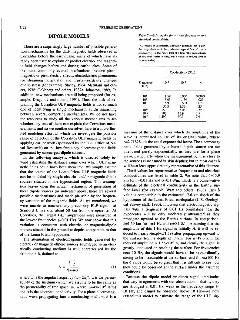
Table 2.-Skin depths for various frequencies and electrical conductivities
[All values in kilometers. Seawater generally has a con- ductivity close to 4 Slm, whereas typical "earth" has a conductivity in the range 0.01-0.1 Slm. The conductivity of dry rock varies widely, but a value of 0.0001 Slrn is representative]
Conductivity (Slm)
Frequency 1&-4 10-I 4 (Hz)
measure of the distance over which the amplitude of the wave is attenuated to 11e of its original value, where e=2.71828 ... is the usual exponential factor. The electromag- netic fields generated by a buried dipole source are not attenuated purely exponentially, as they are for a plane wave, particularly when the measurement point is close to the source (as measured in skin depths); but in most cases 6 will be at least approximately representative of this distance.
The 6 values for representative frequencies and electrical conductivities are listed in table 2. We note that 6=15.9 km for f=0.01 Hz and 0=0.1 Slrn, which is a conservative estimate of the electrical conductivity in the Earth's sur- face layer (for example, Watt and others, 1963). This 6 value is comparable to the estimated 17.6-km depth of the hypocenter of the Loma Prieta earthquake (U.S. Geologi- cal Survey staff, 1990), implying that electromagnetic sig- nals with a frequency of 0.01 Hz originating near the hypocenter will be only moderately attenuated as they propagate upward to the Earth's surface. In comparison, 6=1.59 krn for w=1 Hz and 0=0.1 Slrn. Assuming that the amplitude of this 1-Hz signal is initially A, it will be re- duced to nearly Aexp(-dl1.59) after propagating upward to the surface from a depth of d km. For d=17.6 km, the reduced amplitude is 1.56xlO-q, and clearly the signal is greatly attenuated on reaching the surface. For frequencies near 10 Hz, the signals would have to be extraordinarily strong to be measurable at the surface, and for roslOO Hz the 6 value would be so great that it is difficult to see how they could be observed at the surface under the assumed conditions.
Because the dipole model produces signal amplitudes that vary in agreement with our observations-that is, they are strongest at 0.01 Hz, weak in the frequency range 1- 10 Hz, and cannot be observed above 10 Hz-we now extend this model to estimate the range of the ULF sig-


C24 PRESEISMIC OBSERVATIONS
generate surface electrical effects or other changes that might launch ELFNLF signals into the atmosphere. Our failure to observe precursory ELFNLF noise so close to the epicenters of four moderate to large earthquakes, and the negative result of the Henderson and others (1991) sat- ellite study, show that ELF/VLF noise need not be a strong or an obvious feature of every earthquake.
Perhaps the most important aspect of the results present- ed here is our identification of the frequency range 0.01-1 Hz as a potential "window" for electromagnetic fields that might be generated by earthquakes at depths in the ap- proximate range 0-30 km. Lower frequency electromag- netic-field fluctuations can also escape without difficulty from sources situated within this depth range (and at greater depths), but the paucity of preearthquake observa- tions of electromagnetic signals with frequencies less than 0.01 Hz suggests that lower frequencies are either not gen- erated or only weakly generated. Further experimental and theoretical studies to investigate the possibility of electro- magnetic precursors to earthquakes in this frequency "win- dow" are clearly desirable.
ACKNOWLEDGMENTS
We thank Kathy Mathew for her assistance with the oper- ation of the Corralitos MA-index generator, and M.J.S. Johnston and W.L. Ellsworth of the U.S. Geological Survey for much helpful information. This research was supported by U.S. Office of Naval Research grants N00014-90-J- 1080 and N00014-92-J-1576 under contract N00014-83- K-0390.
REFERENCES CITED
Bakun, W.H., and Lindh, A.G., 1985, The Parkfield, California, earth- quake prediction experiment: Science, v. 229, no. 4714, p. 619-624.
Bernardi, Arman, 1989, Remote measurements of geomagnetic activity; signal processing in the presence of uncertainties in autocovariance estimates: Stanford, Calif., Stanford University, Ph.D. thesis, 120 p.
Bernardi, Arman, Fraser-Smith, A.C., McGill, P.R., and Villard, O.G., Jr., 1991, ULF magnetic field measurements near the epicenter of the Ms 7.1 Loma Prieta earthquake: Physics of the Earth and Planetary Interiors, v. 68, no. 1-2, p. 45-63.
Bernardi, Arman, Fraser-Smith, A.C., and Villard, O.G., Jr., 1989, Meas- urements of BART magnetic fields with an automatic geomagnetic pulsation index generator: Institute of Electrical and Electronics En- gineers Transactions on Electromagnetic Compatibility, v. 3 1, p. 413-417.
Draganov, A.B., Inan, U.S., and Taranenko, Y.N., 1991, ULF magnetic signatures at the earth surface due to ground water flow; a possible precursor to earthquakes: Geophysical Research Letters, v. 18, no. 6, p. 1127-1130.
Fenoglio, M.A., Fraser-Smith, A.C., and Beroza, G.C., 1991, Search for ultra-low frequency electromagnetic signals during the 1989 Loma Prieta earthquake aftershock sequence [abs.]: Eos (American Geo- physical Union Transactions), v. 72, supp., p. 330.
Fenoglio, M.A., Fraser-Smith, A.C., Beroza, G.C., and Johnston, M.J.S., in press, Comparison of ultra-low frequency electromagnetic signals with aftershock activity during the 1989 Loma Prieta earthquake se- quence: Seismological Society of America Bulletin.
Fraser-Smith, A.C., Bemardi, Arman, McGill, P.R., Ladd, M.E., Helli- well, R.A., and Villard, Jr., O.G., 1990a, Low-frequency magnetic field measurements near the epicenter of the Mr 7.1 Loma Prieta earthquake: Geophysical Research Letters, v. 17, no. 9, p. 1465- 1468.
1990b, ULF, ELF, and VLF electromagnetic field observations close to the epicenter of the Ms 7.1 Loma Prieta earthquake; possi- ble ULF precursors [abs.]: Eos (American Geophysical Union Transactions), v. 71, no. 8, p. 288.
Fraser-Smith, A.C., and Bubenik, D.M., 1980, Compendium of the UL- FjELF electromagnetic fields generated above a sea of finite depth by submerged harmonic dipoles: Stanford, Calif., Stanford Universi- ty, Stanford Electronic Laboratories Report SEL-79-025, 114 p.
Fraser-Smith, A.C., and Helliwell, R.A., 1985, The Stanford University ELF/VLF radiometer project; measurement of the global distribu- tion of ELFNLF electromagnetic noise: Institute of Electrical and Electronics Engineers International Symposium on Electromagnetic Compatibility, 1985, Proceedings, p. 305-31 1.
Fraser-Smith, A.C., Helliwell, R.A., Fortnam, B.R., McGill, P.R., and Teague, C. C., 1988, A new global survey of ELFNLF radio noise: Conference on Effects of Electromagnetic Noise and Interference on Performance of Military Radio Communication Systems, Lisbon, 1987, Proceedings, p. 4A-1 to 4A-9.
Fraser-Smith, A.C., McGill, P.R., Bernardi, Arman, Helliwell, R.A., and Ladd, M.E., 1991, Global measurements of low-frequency radio noise, in Environmental and space electromagnetics: Tokyo, Spring- er-Verlag, p. 191-200.
Gokhberg, M.B., Morgounov, V.A., and Aronov, Y.L., 1981, Radiofre- quency radiation during earthquakes: Akademiya Nauk SSSR Doklady, v. 248, p. 32-35.
Gokhberg, M.B., Gufel'd, I.L., and Dobrovol'skiy, I.P., 1982a, Sources of electromagnetic precursors of earthquakes: Akademiya Nauk SSSR Doklady, v. 250, p. 15-17.
Gokhberg, M.B., Morgounov, V.A., Yoshino, Toshio, and Tomizawa, I., 1982b, Experimental measurement of electromagnetic emissions possibly related to earthquakes in Japan: Journal of Geophysical Re- search, v. 87, no. B9, p. 7824-7828.
Henderson, T.R., Sonwalker, V.S., Helliwell, R.A., Inan, U.S., and Fra- ser-Smith, A.C., 1991, A search for ELFNLF emissions induced by earthquakes as observed in the ionosphere by the DE-2 satellite [abs.]: Eos (American Geophysical Union Transactions), v. 72, supp., p. 330.
Johnston, M.J.S., 1989, Review of magnetic and electric field effects near active faults and volcanoes in the U.S.A.: Physics of the Earth and Planetary Interiors, v. 57, no. 1-2, p. 47-63.
Larkina, V.I., Migulin, V.V., Molchanov, O.A., Kharkov, I.P., Inchin, A.S., and Schvetcova, V.B., 1989, Some statistical results on very low frequency radiowave emissions in the upper ionosphere over
. earthquake zones: Physics of the Earth and Planetary Interiors, v. 57, no. 1-2, p. 100-109.
Larkina, V.I., Nalivayko, A.V., Gershenzon, N.I., Gokhberg, M.B., Liper- ovskiy, V.A., and Shalimov, S.L., 1983, Observations of VLF emis- sion, related with seismic activity, on the Interkosmos-19 satellite: Geomagnetism and Aeronomy, v. 23, p. 684-687.
Mizutani, Hitoshi, Ishido, Tsuneo, Yokokura, Takanobu, and Ohnishi, Shuhei, 1976, Electrokinetic phenomena associated with earth- quakes: Geophysical Research Letters, v. 3, no. 7, p. 365-368.
Oike, Kazuo, and Ogawa, Toshio, 1982, Observations of electromagnetic radiation related with the occurrence of earthquakes: Kyoto, Japan, Kyoto University, Disaster Prevention Research Institute Annual Report, v. 25, no. B-1, p. 89-100.

ANALYSIS OF LOW-FREQUENCY-ELECTROMAGNETIC-FIELD MEASUREMENTS NEAR THE EPICENTER C25
Parrot, M., and Mogilevsky, M.M., 1989, VLF emissions associated with earthquakes and observed in the ionosphere and the magnetosphere: Physics of the Earth and Planetary Interiors, v. 57, p. 86-99.
Rikitake, Tsuneji, 1975, Earthquake prediction: Amsterdam, Elsevier, 357 p.
Serebryakova, O.N., Bilichenko, S.V., Chmyrev, V.M., Parrot, M., Rauch, J.L., LeFeuvre, F., and Pokhotelov, 0. A., 1992, Electromagnetic ELF radiation from earthquake regions as observed by low-altitude satellites: Geophysical Research Letters, v. 19, no. 2, p. 91-94.
Shapiro, V.A., and Abdullabekov, K.N., 1982, Anomalous variations of the geomagnetic field in East Fergana-magnetic precursor of the Alay earthquake with M-7.0 (1978 November 2): Royal Astronomi- cal Society Geophysical Journal, v. 68, no. 1, p. 1-5.
Stacey, F.D., 1964, The seismomagnetic effect: Pure and Applied Geo- physics, v. 58, no. 1, p. 5-22.
Tate, Joseph, and Daily, William, 1989, Evidence of electro-seismic phe- nomena: Physics of the Earth and Planetary Interiors, v. 57, no. 1-2, p. 1-10.
U.S. Geological Survey staff, 1990, The Loma Prieta, California, earth- quake; an anticipated event: Science, v. 247, no. 4940, p. 286-293.
Varotsos, P., and Lazaridou, M., 1991, Latest aspects of earthquake pre- diction in Greece based on seismic electric signals: Tectonophysics, v. 188, no. 3-1, p. 321-347.
Watt, A.D., Mathews, F.S., and Maxwell, E.L., 1963, Some electrical characteristics of the earth's crust: Institute of Electrical and Elec- tronics Engineers Proceedings, v. 51, no. 6, p. 897-910.


C28 PRESEISMIC OBSERVATIONS
DATA The magnetometer stations were not operational at the
time of or during the 3-year period before the earthquake, and so details of preseismic effects, if any, are unavailable. Because these data are obtained by using drift-free magne- tometers and are extremely stable over time, comparison of pre-1986 with postseismic data would allow identifica- tion of the net magnetic-field offset that occurred with the earthquake. To isolate local magnetic-field changes and re- duce the effects of ionospheric and magnetospheric distur- bances, synchronously sampled magnetic-field data from pairs of sites are differenced and averaged, and secular variation is removed. For example, 3-day averages of data referenced to station SJN (fig. 1) are plotted in figure 2. Comparison of data collected before 1986 with data ob- tained during the months after the earthquake indicate off- sets of 0.1 to 1.4 nT (table 1). The largest changes were observed at the stations located nearest the epicenter of the earthquake; standard deviations of these data range from 0.2 to 0.6 nT. To test this procedure of extrapolating from 1986 to 1989, continuous differenced data from pairs of stations with similar separations but at large (>I00 km) distances from the Loma Prieta region were subjected to identical processing, using data over the same time period (1983-present). Comparison of these data both with and without the 3-year data gap indicate that offsets estimated in this manner could be biased by as much as 0.7 nT.
Table 1 .-Predicted and observed changes in total magnetic field, refer- enced to station SJN (fig.]), as a function of distance from the epicenter of the Loma Prieta earthquake
[Errors shown for observed values are standard deviations of pre-1986 data. All observed values are within 0.7 nT of predicted values]
Station Predicted Observed Difference Distance (nT) (nT) observed minus (km)
predicted (nT)
EUC -1.1 -1.4k0.2 -0.3 7.3
SAR -1.4 -1.3 * 0.2 M. 1 28.3
NAN -0.5 -1.1 k 0.4 -0.6 3.9
ANZ -0.5 M.1 Â 0.6 M.6 3.9
SNJ -0.2 -0.3 k 0.1 -0.1 36.1
SJN Reference 41.9
HAR M.1 -0.6 Â 0.1 -0.7 49.2
LEW M.2 M.l k 0.1 -0.1 68.2
1984' 1986' 1988' YEARS
Figure 1.-Loma Prieta region, Calif., showing locations of magnetome- ter stations (dots) relative to epicenter of earthquake (star). Lines, major faults; heavy line, Loma Prieta rupture zone. Arrows denote direction of fault movement.
Figure 2.-Processed magnetic-field data from stations EUC (A), SAR (B), SNJ (C), and LEW (D), showing offsets between pre-1986 and post- seismic data referenced to station SJN (see fig. 1 for locations). All data are displayed with identical vertical scale, and plots from top to bottom represent increasing distance from epicenter of earthquake.

1 SEISMOMAGNETIC EFFECTS C29
DISCUSSION
Coseismic magnetic-field offsets can result from piezo- magnetic effects generated by an earthquake-related change in the local stress field. Estimates of the stress change from dislocation models of the earthquake were combined with a seismomagnetic model to calculate the expected magnetic-field change for the earthquake. This model was constructed for an earthquake in which the strike, dip, depth, fault length, fault width, and style of faulting were chosen to be consistent with the geodetically determined parameters (fig. 3; Plafker and Galloway, 1989). Aeromagnetic data indicate a magnetic high in the epicentral region of the earthquake; this anomaly was in- ferred to be caused by buried plutonic rocks similarto the gabbro exposed near station ANZ (fig. 1; Hanna and oth- ers, 1972). Magnetic measurements on the gabbro exposed near station ANZ indicate magnetizations of 2 to 3 Alm, whereas other rock types in the region ranged in magneti- zation from 0.01 to 0.7 A/m. For modeling purposes, a value of 1.5 A/m was chosen to represent the average re- gional magnetization. The contours of calculated magnet- ic-field change for this model are mapped in figure 3. The observed magnetic-field offsets can be approximately fitted by this seismomagnetic model of the earthquake (table 1). If anything, the model values systematically underestimate
isco,
' FAULT-MODEL PARAMETERS 41.8 km
Fault azimuth 131.73 70 SW 6.0 km
'-TI\ \ 12.8 km Strike-slip component 1.9 m right
Â¥< Lorna \<!\
KILOMETERS
Figure 3.-Loma Prieta region, Calif., showing contours of calculated magnetic-field (in nanoteslas) expected from earthquake. Dots, magne- tometer stations; star, epicenter of earthquake; lines, major faults; heavy line, Loma Prieta rupture zone. Fault parameters used to model event are listed in inset.
the observations but are within the uncertainty of the ob- served values. Minor modifications of the model parame- ters could generate a better fit.
An alternative explanation in terms of an electrokinetic model is possible (Fitterman, 1979) but unlikely. The mag- netic-field offsets have remained invariant for several months, with no indication of decay as the ground-water system stabilized. However, -because some ground-water flow did occur immediately after the earthquake, this proc- ess cannot be completely ruled out.
Large-amplitude electromagnetic fields in the ultra-low- frequency (ULF) ra.nge 0.01-10 Hz were observed near the epicenter of the earthquake (Fraser-Smith and others, 1990). The changes were observed before the earthquake and have continued after it. These ULF magnetic-field measurements were obtained at a site approximately 3 krn south of station EUC (fig. 1) and about the same distance from the hypocenter. The proton-precession magnetome- ters operated in the USGS network have a 10-minute sam- pling interval, measure total-magnetic-field intensity (least count, 0.1 nT), and are not designed to monitor magnetic- field fluctuations at frequencies of 0.01 to 10 Hz. Howev- er, owing to aliasing (Bendat and Piersol, 1966), the effect of 0.5- to 4-nT (A.C. Fraser-Smith, oral commun., 1990) increases in ULF magnetic-field noise could increase the apparent short-period background-noise level recorded by the precession magnetometers.
To search for increases in background noise in the total magnetic-field intensity at station EUC (fig. I), a 17-day section of data from 1984 was compared with a similar section in 1989 after the earthquake. Both sections contain data with similar levels of solar disturbance activity. The magnetic-field intensity at station EUC referenced to sta- tion SJN (fig. 1) is plotted in figure 4A, and power spectra obtained from the two sections of data in figure 4B. Both the differenced data plots and the power spectra indicate no significant differences between the total magnetic field in 1984 and after the earthquake. Total-magnetic-field data during the time period of the largest observed ULF mag- netic-field changes (3-hour period before the earthquake) are unavailable.
CONCLUSIONS
Two physical mechanisms could explain the seismomag- netic effects recorded after the earthquake: (1) The seismic- stress drop caused piezomagnetic effects and consequent local magnetic-field changes, or (2) substantial electrical currents were generated rapidly by either rupture-driven charge-generation mechanisms or earthquake-driven fluid flow (electrokinetic effects). The persistence of these chang- es for periods of months since the earthquake and the high conductivity of the Earth's crust appear to preclude electro- kinetic effects as primary physical mechanisms driving the

C30 PRESEISMIC OBSERVATIONS
changes. The observations are generally consistent in ampli- tude and sense with a reasonable seismomagnetic model of the event. Observed increases in ULF magnetic-field noise near the epicenter of the earthquake were not detected in the total-magnetic-field measurements.
ACKNOWLEDGMENTS
We thank A.C. Fraser-Smith and his colleagues at the STAR Laboratory of Stanford University, Stanford, Calif., for making the ULF magnetic-field records available to us.
0 5 10 15 DAYS
Sl s2
t 5x 1 o ' ~ 5 x 1 0 " ~ 5x11 o - ~
(20000 MIN) (2000 MIN) (200 MIN) (20 MIN)
FREQUENCY (C.P.M.)
Figure 4.-Comparative 17-day sections of magnetic-field data from sta- tion EUC referenced to station SJN (fig. 1) during 1984 (A) and 1989 (B), with corresponding power spectra (C and D, respectively). 95-per- cent-confidence limits in figures 4A and 4 5 are 12.1 and -5.1 db, respec- tively. Dominant power in figures 4C and 4D is at solar-spectral peaks S, and Sy.
REFERENCES CITED
Bendat, J.S., and Piersol, A.G., 1966, Measurements and analysis of ran- dom data: New York, John Wiley & Sons, 390 p.
Breiner, Sheldon, and Kovach, R.L., 1967, Local geomagnetic events as- sociated with displacements on the San Andreas fault: Science, v. 158, no. 3797, p. 116-118.
Davis, P.M., Jackson, D.D., and Johnston, M.J.S., 1980, Further evidence of localized geomagnetic field changes before the 1974 Thanksgiv- ing Day earthquake, Hollister, California: Geophysical Research Letters, v. 7, no. 7, p. 513-516.
Fitterman, D.V., 1979, Theory of electrokinetic-magnetic anomalies in a faulted half-space: Journal of Geophysical Research, v. 84, no. B 1 1, p. 6031-6040.
Fraker-Smith, A.C., Bernardi, Arrnan, McGill, P.R., Ladd, M.E., Helli- well, R.A., and Villard, O.G., Jr., 1990, Low-frequency magnetic field measurements near the epicenter of the Ms 7.1 Loma Prieta earthquake: Geophysical Research Letters, v. 17, no. 9, p. 1465- 1468.
Hanna, W.F., Brown, R.D., Jr., Ross, D.C., and Griscom, Andrew, 1972, Aeromagnetic reconnaissance and general geology map of the San Andreas fault between San Francisco and San Bernardino, Califor- nia: U.S. Geological Survey Geophysical Investigations Map GP- 8 15, scale 1 :250,000.
Honkura, Yoshimori, and Taira, S., 1983, Changes in the amplitudes of short-period geomagnetic variations as observed in association with crustal uplift in the Izu Peninsula, Japan: Earthquake Prediction Re- search, v. 2, no. 2, p. 115-125.
Johnston, M.J.S., 1986, Local magnetic fields, uplift, gravity, and dila- tional strain changes in southern California: Journal of Geomagne- tism and Geoelectricity, v. 38, no. 10, p. 933-947.
Johnston, M.J.S., and Mueller, R.J., 1987, Seismomagnetic observation during the 8 July 1986 magnitude 5.9 North Palm Springs earth- quake: Science, v. 237, no. 4819, p. 1201-1203.
Mueller, R.J., Johnston, M.J.S., Smith, B.E., and Keller, V.G., 1981, U.S. Geological Survey magnetometer network and measurement tech- niques in western U.S.A.: U.S. Geological Survey Open-File Report 81-1346,44 p.
Nagata, T., 1970, Basic magnetic properties of rocks under the effect of mechanical stresses: Tectonophysics, v. 9, p. 167-195.
Ohshiman, Naoto, Sasai, Yoichi, Ishikawa, Yoshinobu, Honkura, Yoshi- mori, and Tanaka, H., 1983, Local changes in the geomagnetic total intensity associated with crustal uplift in the Izu Peninsula, Japan: Earthquake Prediction Research, v. 2, no. 3, p. 209-219.
Plafker, George, and Galloway, J.P., eds., 1989, Lessons learned from the Loma Prieta, California, earthquake of October 17, 1989: U.S. Geo- logical Survey Circular 1045,48 p.
Rikitake, Tsuneji, 1979, Changes in the direction of magnetic vector of short-period geomagnetic variations before the 1972 Sitka, Alaska, earthquake: Journal of Geomagnetism and Geoelectricity, v. 31, no. 4, p. 4 4 1 4 5 .
Shapiro, V.A., and Abdullabekov, K.N., 1982, Anomalous variations of the geomagnetic field in East Fergake-magnetic precursor of the Alay earthquake with M=7.0 (1978 November 2): Royal Astronomi- cal Society Geophysical Journal, v. 68, no. 1, p. 1-5.
Smith, B.E., and Johnston, M.J.S., 1976, A tectonomagnetic effect ob- served before a magnitude 5.2 earthquake near Hollister, California: Journal of Geophysical Research, v. 81, no. 20, p. 3556-3560.
Stacey, ED., 1964, The seismomagnetic effect: Pure and Applied Geo- physics, v. 58, p. 5-22.

THE LOMA PRIETA, CALIFORNIA, EARTHQUAKE OF OCTOBER 17,1989: EARTHQUAKE OCCURRENCE
PRESEISMIC OBSERVATIONS
NEAR-SOURCE SHORT- TO INTERMEDIATE-PERIOD GROUND MOTIONS
By Randall A. White and William L. Ellsworth, U.S. Geological Survey
CONTENTS
Abstract - ................................................................... Introduction ................................................... --- ----- ----- Seismic-&~ acquisition and analysis - ....................... - -------- Microearthquake activity before the main shock .................... Moving-window spectral analysis --------------------------am---------
The search for correlated noise- -------------------- - ------- - ----------- Discussion ÑÑÑÑ------------------------------------------Ñ-F-- Conclusions- ............................................................... Acknowledgments-------------------------------------------------------- References cited .......................................................... Supplementary information: nontectonic sources of seismic
noise .................................................................... Animals walking - .................................................. Motor vehicles ...................................................... Trains ................................................................. Aircraft ............................................................... Weather .............................................................. Electric-power stations ............................................ Private electric generators, construction sites, and
miscellaneous sources ------------------------------------------
ABSTRACT
Page
C3 1 3 1 13 33 34 37 39 42 43 43
44 44 45 45 45 45 45
45
We have examined short- to intermediate-period ground motions recorded in the epicentral vicinity of the earthquake for evidence of any naturally occurring seismic signals dur- ing the 7%-hour period immediately before the main shock. Standard telemetered U.S. Geological Survey short-period- seismographic stations measure ground noise in the band 0.1 to about 20 Hz and can detect local earthquakes as small as MasO.0. Power-spectral densities of ground-motion noise were computed for consecutive 2.73-minute windows at three stations within 7 km of, one station about 35 km from, and one station about 70 km from the epicenter. There is no discernible change in seismic power over the range 0.1-5.0 Hz with the approach of the main shock.
We also examined records from the three stations clos- est to the epicenter for evidence of correlated energy, but none was observed. During this period, energy in the fre- quency ranges near 2-3 Hz and 10-13 Hz predominates, much of which can be traced to cultural sources, particu-
larly the energy above 8 Hz. Seismograms with nearly identical spectral characteristics were also recorded at these same stations on randomly selected dates more than 2 years before and 4% months after the earthquake, suggest- ing that nothing in the spectra during the 7%-hour period before the main shock derives from the impending event. From October 1, 1989, until the main shock, only seven earthquakes, none larger than Mz1.5, occurred within 10 km of the eventual aftershock zone. All seven of them oc- curred near the ends of the aftershock zone. Two of these earthquakes (M=0.8 and 1.2), which occurred only 3% hours before the main shock, nevertheless appear to be normal aftershocks of the August 8, 1989, Lake Elsman earthquake (M=5.2).
INTRODUCTION
The motivation for this study was to discover any fore- shocks or other short-term seismic signals that might pro- vide evidence for short-term precursory changes in the focal volume surrounding the main shock. To this end, we searched all the analog records from 21 stations located within 20 km of the main-shock epicenter, looking for rni- croearthquakes as small as M=0.0 during the 7%-hour peri- od before the main shock, and performed spectral analysis on the seismic data from 5 stations located 7 to 70 km from the epicenter, looking for changes in the amplitude of ground-motion noise and for correlated seismic noise over the useful bandwidth of standard U.S. Geological Survey (USGS) seismic stations, from 0.1 to 5 Hz. We found no foreshocks, changes in seismicity patterns, or any other anomalous seismic signals during this period that could be construed as possible seismic precursors to the earthquake.
SEISMIC-DATA ACQUISITION AND ANALYSIS
The USGS operates about 350 telemetered short-period- seismographic stations in northern and central California.

C32 PRESEISMIC OBSERVATIONS
At the time of the earthquake, 21 of these stations were located within 20 km of the epicenter, including 1 located within 1 km of the epicenter (fig. 1). The frequency-modu- lated (FM) analog signals from seismic stations are telem- etered to the USGS offices in Men10 Park, Calif., where they are continuously recorded on 9,600-ft-long, 1-in.- wide, 14-track magnetic tape. One tape is recorded each day on one of five continuously recording tape drives. The seismic signals are also digitized in realtime at 100 sam- ples per second, but only time windows containing local events are preserved (see fig. 5C, see Baton, 1977, for a more complete description of the USGS seismic-data ac- quisition and archiving scheme). Despite the severe low-
frequency rolloff, typical USGS seismic stations can detect measurable seismic energy at frequencies as low as 0.1 Hz. Data presented below will show that these short-peri- od-seismographic stations detect measurable seismic ener- gy in the frequency range 0.1-10 Hz.
This FM-tape system was designed to routinely record waveforms of earthquakes as small as M=l, as a backup to digital recording of earthquakes, which preserves only short periods of data containing earthquake seismograms. The daily tapes containing the Loma Prieta main shock were put aside for posterity and survived the normal data-compres- sion process intact; however, no other daily tape, for the 2- month period before the main shock, was retained.
Figure 1.-Loma Prieta region, Calif., showing locations of seismic sta- and dotted lines denote surface traces of faults with Holocene slip, in- tions near the Loma Prieta rupture zone. Stars, standard U.S. Geological ferred faults with Holocene slip, and suspected faults, respectively. ML, Survey short-period-seismographic stations: large stars with three-letter Moss Landing power station; SF BAY, San Francisco Bay; TV, television station codes, four of the five stations used in this study (the fifth station, transmission tower; ULF-EM, ultra-low-frequency electromagnetic re- BPR, is located 30 km to the south, outside map area). Solid, dashed, ceiver; WJ, Watsonville Junction.

mAR-SOURCE SHORT- TO INTFiRMEDMTE-PERIOD GROUND MOTIONS c33
MICROEARTHQUA= ACTIVITY BEFORE THE MAIN SHOCK
Seismicity in the San Francisco-Monterey Bay region in the 20-year period before the earthquake was studied by Olson (1990, p. 1430), who pointed out that "While some small events did occur along the Loma Prieta rupture zone in the seven weeks preceding the Loma Prieta earthquake, none of these were observed to be unusual when com- pared to the spatial distribution of the relocated seismicity since 1980."
Looking at the time period from October 1 until the main shock in more detail, we find that only seven earth- quakes, none larger than M=l.S, occurred within 10 km of the eventual Loma Prieta aftershock zone (fig. 2). Four of
these earthquakes occurred near the southeast end of the aftershock zone, and the other three, which are aftershocks of the August 8, 1989, Lake Elsman earthquake, occurred within the northwest end of the aftershock zone. The northernmost pair of these aftershocks occurred during the 7%-hour peri~d before the main shock, as we discuss in more detail below. The small cluster of earthquakes a few kilometers east of the San Andreas fault (upper corner, fig. 2) are noteworthy in that this area became highly active after the main shock: More than 90 events occurred there during the first 2 weeks of the aftershock sequence. The pre-main-shock cluster, however, was comparable in both the number of events and their magnitudes to several other sequences that occurred there during the preceding 20 years.
I I I I I I I
SF BAY EXPLANATION
MAGNITUDE
Figure 2.-Loma Prieta region* Calif.* showing seismicity near main-shock epicenter during the period October 1-17, 1989. Note that no events of M23 occurred in the region during this period. Two northernmost events within aftershock zone occurred 3% hours before main shock. See figure 1 for explanation of faults.

c34 PRESEISMIC OBSERVATIONS
In the rest of this section, we examine seismic activity during the 7%-hour period before the main shock (the dai- ly tapes containing the main shock begin at 1647 G.m.t. October 17). Analog records for this period were prepared on strip-chart paper at a speed of 6 c d s , using a low-pass filter with a corner at 16 Hz, which rolls off at 12 dB/oc- tave, to remove system noise, and a high-pass filter with a corner at 0.1 Hz, which rolls off at 6 dB/octave, to remove dc drift (Eaton, 1980). These records were carefully scanned for any seismic signals that may have been missed by either the human record readers or the automat- ic earthquake-detection algorithm. Normally, the seismic network can locate events as small as Ms0.5; however, by visually scanning the most sensitive stations in the area, we find that events as small as Ms0.0 can be detected in most areas along the eventual aftershock zone.
The only two microearthquakes that we identified during this period were the two Lake Elsman aftershocks dis- cussed above, which occurred 4 s apart about 3% hours before the main shock. The events originated near the northwest base of the rupture zone, 12 km beneath Lake Elsman. Waveforms of these events are shown in figure 3. These two microearthquakes have magnitudes of 0.8 and 1.2 and, owing to their small sizes, could not be detected at stations farther than about 30 km from Lake Elsman.
The only other signals that appear to be of tectonic ori- gin occurred at 1852 G.m.t. (fig. 4A). These signals cannot be seen clearly at any station other than JEC. If they are of tectonic origin, the magnitude of the largest event is about 0.0.
Next, we assembled a second set of continuous records for this period by passing the seismograms through a high- pass filter with a comer at 0.5 Hz, which rolls off at 12 dB/octave. Several types of seismic signals other than earthquakes are visible in these records (fig. 4). Of those signals whose sources can be traced, all are of cultural ori- gin, almost all from motor vehicles. Other sources known to produce seismic noise include moving animals, trains, aircraft, electric-power generators, construction sites, weather (including wind, rain, and hail), and flowing water. High-tension lines and radio and television trans- mitters can also generate electric currents along the ground surface that can, in turn, induce erroneous signals within the station transducers. In the supplementary section be- low, we summarize investigations into nontectonic sources of seismic noise in the vicinity of the earthquake.
Although the specific origin of many of the seismic sig- nals recorded during the hours before the main shock re- mains unclear, visual inspection of records for randomly selected dates long before and after the earthquake show similar signals. Specifically, we examined continuous FM tapes recorded on September 9, 1987, and March 3, 1990. For both dates, we produced 1-hour-long paper records at 6 c d s from 2300 to 0000 G.m.t., the time of day corre- sponding to the hour before the main shock. From the sec-
ond tape, we also produced an additional, 45-minute-long paper record for the time beginning at 0700 G.m.t. (mid- night local time) March 4, when cultural noise is very low. Visual comparison of the records from immediately before the main shock with the records from September 1987 and March 1990 shows many similarities, especially among the relatively short bursts of energy at frequencies of 2-4 and 10-13 Hz, indicating that these signals were not gen- erated by any process related to the earthquake. The record from March 4, 1990, recorded just after midnight local time, contains much less seismic noise overall and supports the notion that most of the aforementioned ener- gy is of cultural origin.
MOVING-WINDOW SPECTRAL ANALYSIS
To more fully examine the seismograms recorded in the 7%-hour period before the main shock, we use moving- window spectra to search for signals not seen in visual inspection of the records. Analog records were digitized at 100 samples per second from five stations: three, JBZ, JEC, and JPL, 5 to 7 km from the epicenter (fig. 1); one, HOR, about 35 km from the epicenter; and one, BPR, about 70 km from the epicenter. For control, we similarly digitized 1-hour-long sections of the record from station JBZ for September 30, 1987, and March 3, 1990. Both of these sections of record are for the time of day beginning at 2300 G.m.t., corresponding approximately to the hour immediately before the main shock, which is during the local afternoon rush-hour commute. The September 1987 record was chosen, in part, because it was recorded during the same season of the year (during the local apple har- vest) as the main shock. We also digitized a 5-minute-long section of the record from station JBZ for March 4, 1990, beginning at 0700 G.m.t., which corresponds to midnight local time, when cultural noise is very low. Using these data sets, we can compare the power spectra from the nearby stations with (1) those from more distant stations during the same period of time and (2) those from a near- by station at times long before and long after the main shock.
To illustrate these steps in our analysis, we examine a 163.84-s-long sample of relatively quiet record from sta- tion JBZ ending 10 minutes before the main shock (fig. 5A). A few, very small bursts of noise are apparent. For the reasons discussed below, we believe that these noise bursts are of cultural origin. The resulting power spectra, uncorrected for instrumental response, are plotted in figure 5B, and the total instrumental response in figure 5C (for a discussion of the limits of this type of seismic instrumen- tation, see Riedesel and others, 1990). To estimate the power spectrum, we first apply a cosine taper to 5 percent of each end of the window and then compute the period-

1 NEAR-SOURCE SHORT- TO INTERMEDIAm-PERIOD GROUND MOTIONS c35 I ogram, using the fast Fourier transform (FFT) method. ing spectral estimate is 0.013 Hz. The power-spectra1 den-
Variation in the estimated spectrum is further reduced by sity, corrected for instrumental response, is plotted in smoothing this periodogram. The bandwidth of the result- figure 5D.
I
JSSM V "5 s$ +p2 p 2 Distances 1 Azimuths 327 'T 11s . . a . , , I I , a ," - Distance= 7 Azimuth- 92 1
1 0.1
JHLM V Distances 10 Azimuth- 125 - . -- -I 0.1
JSTM V r Distance= 12 Azimuth- 66 u
JRGM V A
Distance= 14 Azimuth= 195 1 0 . 1
JTGM V Distance- 15 Azimuth= 164
P M V Di t n e 2 ' u h 158 1 0 . 1
CCOM V DistahceL 25 Azimuths 64 vL -
10 Seconds
Figure 3.-Waveforms for two events that occurred about 3% hours before main shock, showing 30-s-long records starting 6 s before first event, which originated at 2045:28.65 G.m.t. October 17. Four letter station code and component code are shown at left. P, P-wave onset; S, S-wave onset. At right end of each trace is a vertical scale bar appropriate for ground velocities at 10 Hz; note that bars range in length from 0.01 to 1.0 vm/s. -0 events of M=0.8 and 1.2 originated about 4.5 s apart at depth of 12 km beneath Lake Elsman, near northwest base of Lorna Prieta rupture zone. These events, which are the only earthquakes of M9.0 that occurred during the 7%-hour period before the main shock within the eventual aftershock zone, are aftershocks of the August 8, 1989, Lake Elsman earthquake (Mz5.2).
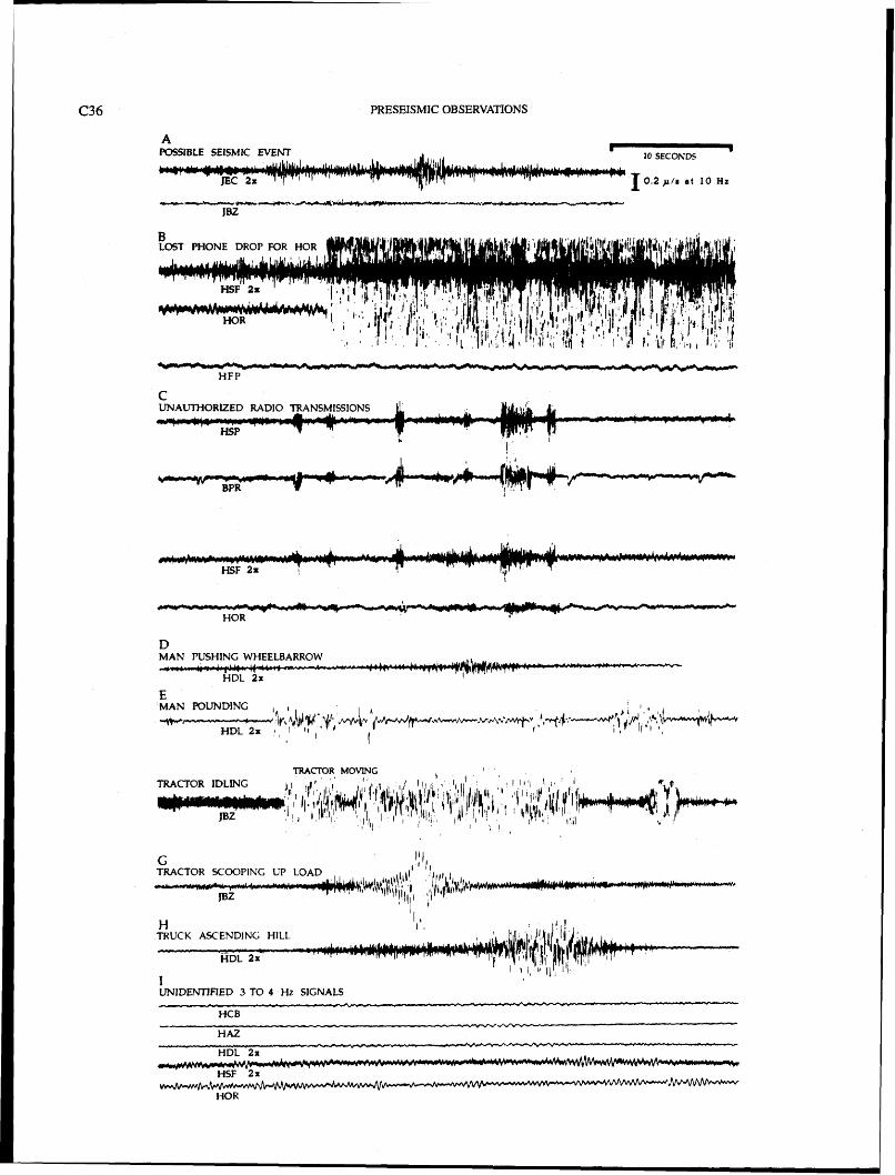
PRESEISMIC OBSERVATIONS
A KXSIBLE SEISMIC EVENT
!ST PHONE DROP FOR HOR fi
TRACTOR MOVING I
1
UNIDENTIFIED 3 TO 4 Hz SIGNALS
- -
HOR

mAR-SOURCE SHORT- TO INTFiRMEDIATE-PERIOD GROUND MOTIONS c37
Spectra obtained during all the above-mentioned time periods exhibit a form similar to this example, with very high spectral levels at the lowest frequencies and some- what-elevated spectral levels at the highest frequencies. For comparison, corrected spectra for typical periods of high and low true ambient seismic noise (Aki and Rich- ards, 1980, v. 1, p. 497) are also plotted in figure 5D.
To illustrate the actual system noise and its effects on the corrected spectra of true seismic noise, the spectra of a "step test," during which the geophone at station JPL was disconnected, are plotted in figure 6. This system noise is due to the combined effects of telemetry and amplifier noise. Also plotted in figure 6 are two sections of record containing seismic signals: (1) the first 2.5 minutes of the main shock at station JPL (the record is clipped) and (2) a section of quiet record from about 1 hour before the main shock. From the fact that the spectra for these two record sections behave as typical seismic noise, except at the high and low ends of the frequency range, where they follow the instrumental-noise spectra, we conclude that between 0.1 and 2.0 Hz we are detecting true seismic noise. When the seismic-to-electronic-noise ratio is large, we are able to detect seismic noise up to 20 Hz.
To investigate the temporal variation of the spectra, we divided the spectral band from 0.1 to 10 Hz into six fre- quency bands, as follows: 0.1-0.2 Hz, 0.2-0.5 Hz, 0.5-1.0 Hz, 1.0-2.0 Hz, 2.0-5.0 Hz, and 5.0-1 0.0 Hz. The average value of the power-spectral density within each frequency band was computed for each 163.84-s-long record section. A total of about 900 spectra were computed. The average values of the power-spectral density within each frequency band for consecutive 163.84-s windows at two stations within 7 km of, three stations about 35 km from, and one station about 70 km from the epicenter are plotted in fig- ure 7. Power-spectral densities, within each of the four frequency bands between 0.1 and 2.0 Hz, fluctuate ran- domly by a factor of less than 4 during the 7%-hour period before the main shock. In no case do we observe changes greater than a factor of 6 at these stations during this peri- od. Although there is some correlated behavior between spectral bands at a given station (for example, BPR), there
4 Figure 4.-Examples of signals recorded on seismograms fkom October 17, 1989. Horizontal scale and vertical scale, appropriate for ground ve- locity at 10 Hz, is shown at top right; station code followed by "2x9* indicates that vertical scale is twice that shown at top right. A, 1852 G.m.t.: only possible seismic events other than those shown in figure 3 may be these signals recorded at station JEC (fig. 1) only (M~0.0). B, 1719 G.m,t.: lost telephone drop for station HOR (fig. 1). C, 1839 G.m.t.: unauthorized radio transmissions interfere with U.S. Geological Survey receiver. D, 1900 G.m.t.: man pushing wheelbarrow. E, 1952 G.m.t.: man pounding. F, 2350 G.m.t.: tractor (idling at 800 rpm generated 13.3-Hz signal shown at each end, moving generated middle signal). G, 1946 G.m.t.: tractor scooping up load. H, 1859 G.m.t.: pickup truck ascending hill, then stopping. 1, Stations HCB, HAZ, and HDL at 1854 G.m.t., and stations HSF and HOR at 1832 G.m.t: unidentified 3- to 4-Hz signals.
is little evidence of correlated behavior between stations. Therefore, we conclude that the small seismic power-spec- tral-density fluctuations observed during the 7%-hour peri- od before the earthquake are in no way unusual and probably are unrelated to the impending earthquake.
The power spectra for station JBZ, nearest the epicenter and neaxest the ultra-low-frequency electromagnetic (ULF- EM) receiver (Fraser-Smith and others, 1990) are plotted in figure 8. These spectra include a 1-hour period on Sep- tember 9, 1987, a 1-hour period on March 3, and a 45- minute period just after midnight local time on March 4, 1990. Note the spikes in the higher-frequency bands. In those cases that can be verified, simultaneous large-ampli- tude spikes within the upper three frequency bands (2.0-20 Hz) correspond to times when motor vehicles passed with- in a few hundred meters of the station. During the 3-hour period immediately before the main shock, the missing data correspond to periods of intense cultural noise gener- ated by a tractor operating within 100 m of the station. The earlier missing data, ending 6.05 hours before the main shock, correspond to a 30-minute period during which a telemetry dropout occurred. Spectra for three other 163.84- s windows, when motor-vehicle noise dominates the ana- log records, were discarded. Of the remaining 120 win- dows, several contain short bursts of cultural noise less than about 20 s long. The most suggestive trend in the spectral levels is a gradual decrease within the band 0.5- 1.0 Hz by a factor of 2 to 3 during the hours before the earthquake. Looking at the data from September 1987 and March 1990, however, similar-size fluctuations apparently occur during the course of days when no significant earth- quakes occur. Therefore, we conclude that no noteworthy changes occur in the seismic power-spectral densities with- in the range 0.1-2.0 Hz at station JBZ during the 7%-hour period before the main shock.
THE SEARCH FOR CORRELATED NOISE
In this section, we examine the possibility that seismic waves of tectonic origin are present but below the ampli- tude of background ,noise. Such signals would escape de- tection by the methods used in the previous section. To search for such signals, we examine pairs of stations for evidence of correlated events, as indicated by cross-spectral coherency. The square of the coherency may be interpreted as the square of the correlation between the random Fourier coefficients of each series, at each particular frequency.
To perform this analysis, we first resampled the original data at 5 samples per second and divided the result into 102.4 (5 12 sample) segments. Power-spectral amplitudes and cross-spectral coherency were estimated from fast Fourier transforms, using a modified Daniel1 smoothing window with weights of (%, 1, 1, 1, %), resulting in a bandwidth of 0.012 Hz.

PRESEISMIC OBSERVATIONS
1 1 I I I 0 !iOQO 1 0000 15000 2 0 0 ~
SAMPLES (100 SAMPLESISEC) AT JBZ
FREQUENCY (Hz)
0.01 0.05 0.1 0.5 1 5 10 5 0 FREQUENCY (Hz)
0.01 0.05 0.1 0.5 1 5 10 !X
FREQUENCY (HZ)
Figure 5.-Time series, instrument response, and corrected power-spectral density from sta- tion JBZ. A, Relatively quiet, 163.84-s-long sample window ending 10 minutes before main shock. B, Uncorrected (relative) power spectra for section of record shown in figure 5A. C, Total instrumental displacement response to ground velocity for a VCO amplifier attenuation setting of 12 dB (most stations are set to either 12 or 18 dB). D, Power-spectral densities relative to 1.0 cm2/Hz, corrected for instrument response, for three different cases: upper Uagged) curve, spectrum for section of record shown in figure SA; upper and lower smooth curves, spectra for periods of high ("noisy")- and low ("quiet")-amplitude true ambient seis- mic noise (from Aki and Richards, 1980).
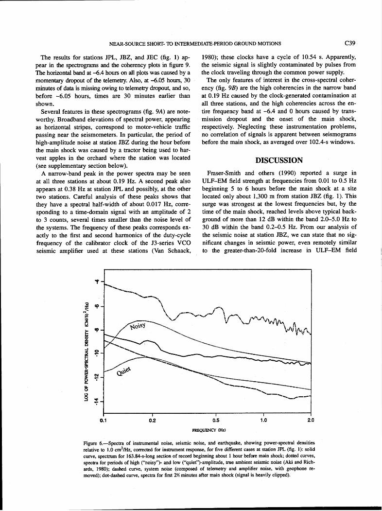
NEAR-SOURCE SHORT- TO INTEMEDIATE-PERIOD GROUND MOTIONS c39
The results for stations JPL, JBZ, and JEC (fig. 1) ap- pear in the spectrograms and the coherency plots in figure 9. The horizontal band at -6.4 hours on all plots was caused by a momentary dropout of the telemetxy. Also, at -6.05 hours, 30 minutes of data is missing owing to telemetry dropout, and so, before -6.05 hours, times are 30 minutes earlier than shown.
Several features in these spectrograms (fig. 9A) are note- worthy. Broadband elevations of spectral power, appearing as horizontal stripes, correspond to motor-vehicle traffic passing near the seismometers. In particular, the period of high-amplitude noise at station JBZ during the hour before the main shock was caused by a tractor being used to har- vest apples in the orchard where the station was located (see supplementary section below).
A narrow-band peak in the power spectra may be seen at all three stations at about 0.19 Hz. A second peak also appears at 0.38 Hz at station JPL and possibly, at the other two stations. Careful analysis of these peaks shows that they have a spectral half-width of about 0.017 Hz, corre- sponding to a time-domain signal with an amplitude of 2 to 3 counts, several times smaller than the noise level of the systems. The frequency of these peaks corresponds ex- actly to the first and second harmonics of the duty-cycle frequency of the calibrator clock of the J3-series VCO seismic amplifier used at these stations (Van Schaack,
1980); these clocks have a cycle of 10.54 s. Apparently, the seismic signal is slightly contaminated by pulses from the clock traveling through the common power supply.
The only features of interest in the cross-spectral coher- ency (fig. 9B) are the high coherencies in the narrow band at 0.19 Hz caused by the clock-generated contamination at all three stations, and the high coherencies across the en- tire frequency band at -6.4 and 0 hours caused by trans- mission dropout and the onset of the main shock, respectively. Neglecting these instrumentation problems, no correlation of signals is apparent between seismograms before the main shock, as averaged over 102.4-s windows.
DISCUSSION
Fraser-Smith and others (1990) reported a surge in ULF-EM field strength at frequencies from 0.01 to 0.5 Hz beginning 5 to 6 hours before the main shock at a site located only about 1,300 m from station JBZ (fig. 1). This surge was strongest at the lowest frequencies but, by the time of the main shock, reached levels above typical back- ground of more than 12 dB within the band 2.0-5.0 Hz to 30 dB within the band 0.2-0.5 Hz. From our analysis of the seismic noise at station JBZ, we can state that no sig- nificant changes in seismic power, even remotely similar to the greater-than-20-fold increase in ULF-EM field
Figure 6.-Spectra of instrumental noise, seismic noise, and earthquake, showing power-spectral densities relative to 1.0 cm2/Hz, corrected for instrument response, for five different cases at station JPL (fig. 1): solid curve, spectrum for 163.84-s-long section of record beginning about 1 hour before main shock; dotted curves, spectra for periods of high ("noisy*')- and low ("quiet")-amplitude, true ambient seismic noise (Aki and Rich- ards, 1980); dashed curve* system noise (composed of telemetry and amplifier noise, with geophone re- moved); dot-dashed curve* spectra for first 2% minutes after main shock (signal is heavily clipped).
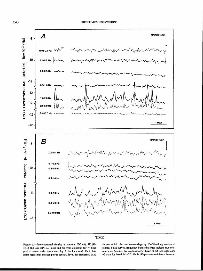
PIESEISMIC OBSERVATIONS
MAIN SHOCK
1 Hour
MAIN SHOCK
1 Hour
TIME
Figure 7.-Power-spectral density at stations JEC (A), JPL(B), shown at left, for one nonoverlapping 164.38-s-long section of HOR (0, and BPR (D) near and far from epicenter for 7%-hour record. Solid curves, frequency bands that best indicate true seis- period before main shock (see fig. 1 for locations). Each data mic noise (see text for explanation). Shown at left and right ends point represents average power-spectral level, for frequency band of data for band 0.1-0.2 Hz is 95-percent-confidence interval,
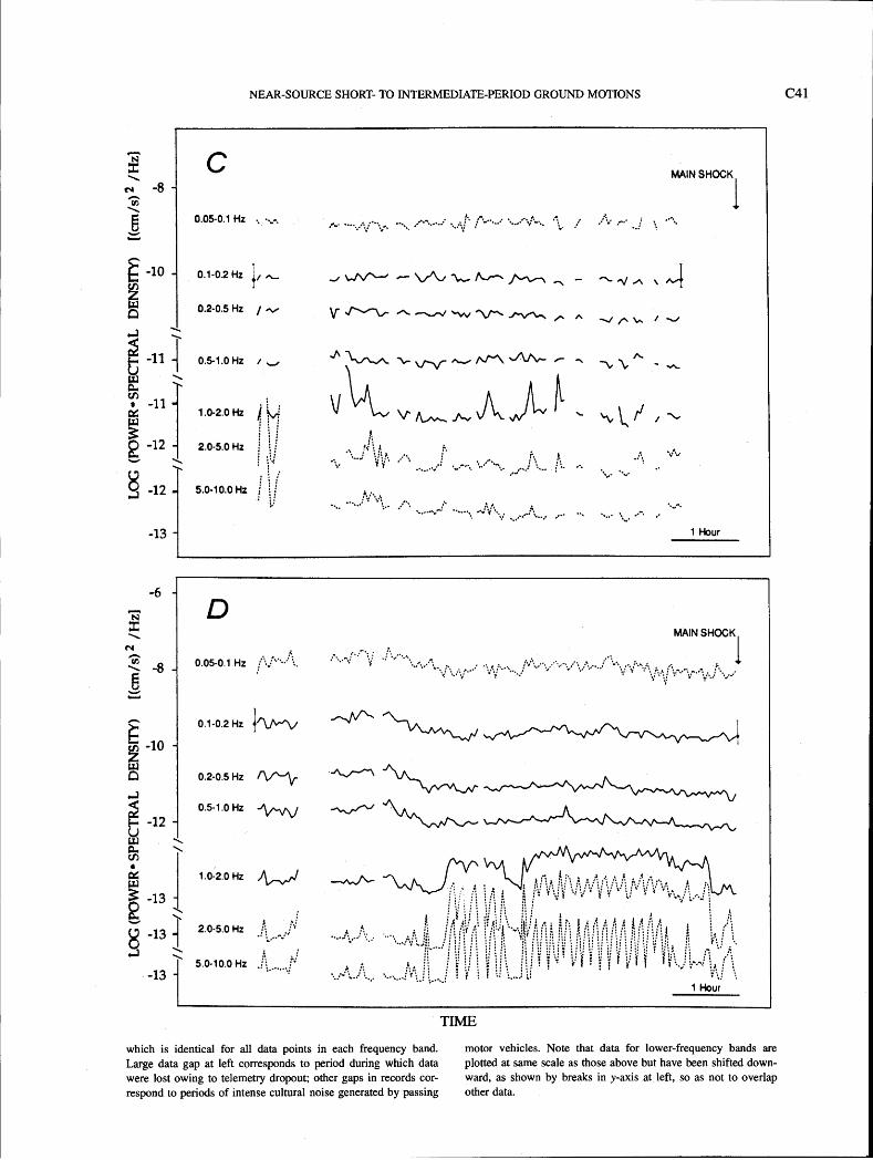
NEAR-SOURCE SHORT- TO INTERMEDIATE-PERIOD GROUND MOTIONS
-13 - 1 Hour
MAIN SHOCK,
1 Hour
TIME
which is identical for all data points in each frequency band. motor vehicles. Note that data for lower-frequency bands are Large data gap at left corresponds to period during which data plotted at same scale as those above but have been shifted down- were lost owing to telemetry dropout; other gaps in records cor- ward, as shown by breaks in y-axis at left, so as not to overlap respond to periods of intense cultural noise generated by passing other data.

C42 PRESEISMIC OBSERVATIONS
strength, occurred over the frequency range 0.1-5.0 Hz during this same period.
Could the October 17, 1989, ULF-EM energy surge have been caused by seismic shaking of the EM sensor? No. Bernardi and others (1991) showed that a horizontal angular rotation of the ULF-EM sensor by 0.02°-0.09 would be required to induce the surge they observed. Any motions of this magnitude, if of tectonic origin, would be readily apparent on the seismic record from station JBZ.
Although the lowest-frequency ranges studied by Fraser- Smith and others (1990) are lower than the detection threshold of the seismic stations studied here, the wave- length of seismic waves corresponding to that range is long enough that it should have shown up on ultrasensitive regional dilatometers. As in this study, no such signals were detected (see Johnston and others, this chapter).
CONCLUSIONS
1. During the 7%-hour period before the main shock, no foreshocks of M>O were detected by the standard USGS short-period-seismographic network.
2. During this period, no significant changes were noted in the power-spectral density of ground motion, at stations near or far from the epicenter, over the frequency band 0.1-10.0 Hz. The few changes detected are smaller than the daily variation seen between times of maximum and minimum cultural noise and are similar to those seen on records from randomly selected dates more than 2 years before and 4 months after the main shock.
3. During this period, there is no correlated seismic ener- gy, over the frequency band 0.1-5.0 Hz, among three stations located within 7 km of the epicenter.
1 Hour
Figure 8.-Power-spectral densities at station JBZ for 1-hour period on September 9, 1987 (left), for 7%-hour period immediately before main shock (middle), and for 1-hour period on March 3, 1990, and 45-minute period on March 4, 1990 (right). See figure 7 for explana- tion of axes, frequency bands, and 95-percent-confidence interval. During 3-hour period immediately before main shock, small gaps in record correspond to periods of intense cultural noise generated by a tractor operating within 100 m of station. 1-hour periods from 1987
TIME
and 1990 are at same time of day as 1-hour period immediately be- fore main shock, which corresponds to local commuter rush hour. 45- minute period on March 4, 1990, begins at midnight local time, when cultural noise levels are very low. High spectral densities in frequen- cy bands above 2 Hz are of cultural origin. Note that differences in spectral densities between rush hour and midnight local time on March 3, 1990, are greater than any changes immediately before earthquake.

NEAR-SOURCE SHORT- TO INTERMEDIATE-PERIOD GROUND MOTIONS C43
ACKNOWLEDGMENTS ing playbacks from analog tapes, and Willie Lee for help in digitizing those tapes. Finally, we thank Nancy King
We thank Tony Fraser-Smith and Arman Bemardi for and Willie Lee for their careful reviews of the manu~cript.
discussions regarding their ULF-EM data and for inspir- ing this study. We thank the landowners, especially at sta- tions JBZ and HDL, upon whose land USGS seismograph
REFERENCES CITED
stations are located, for help in identifying cultural Sources Aki, Keiiti, and Richards, PO., 1980, Quantitative seismology; theory of seismic noise. We thank Jeanie Taylor for help in mak- and methods: San Francisco, W.H. Freeman and Co., 2 v.
Station JPL Station JBZ Station JEC
0.0 0.5 1.0 1.5 2.0 2.5
FREQUENCY, IN HERTZ
Figure 9.-Power spectra at (A) and coherency between (B) stations JPL, JBZ, and JEC (fig. 1) for 7%-hour period before main shock (time is approximate). Final timeline at top of figures contains main shock. Gray scale in figure 9A corresponds to a power-spectral range of approximately 100 dB peak to peak, or about 50 dB in amplitude, with lighter shades representing lower power levels. Dark band at top corresponds to main shock, which is clipped at these stations. Dark band at about -6.4 hours actually corresponds to a 30-minute period during which data were lost owing to telemetry dropout, and so spectral amplitudes before -6.4 hours
are for times 30 minutes earlier than shown. On spectrogram for station JPL, other dark bands before -5 hours, which span entire frequency range shown, correspond to passing motor vehicles. On spectrogram for station JBZ, dark bands between -3 hours and -15 minutes, which span entire frequency range shown, correspond to a tractor operating within 100 m of seismic station. Gray scale in figure 9B represents a range of correlation coefficients from black, representing 1.0 (that is, perfect correlation), to white, representing 0.0 (that is, no correlation). Horizontal bands at about -6.4 hours correspond to a brief data-transmission dropout.

c44 PRESEISMIC OBSERVATIONS
Bernardi, Arman, Fraser-Smith, A.C., McGill, P.R., and Villard, O.G., Jr., 1991, ULF-magnetic field measurements near the epicenter of the Mc 7.1 Loma Prieta earthquake: Physics of the Earth and Planetary Interiors, v. 68, no. 1-2, p. 45-63.
Baton, J.P., 1977, Frequency response of the USGS short period teleme- tered seismic system and its suitability for network studies of local earthquakes: U.S. Geological Survey Open-File Report 77-844,45 p.
1980, Response arrays and sensitivity coefficients for standard configurations of the USGS short-period telemetered seismic sys- tem: U.S. Geological Survey Open-File Report 80-316, 32 p.
Fraser-Smith, A.C., Bernardi, Arman, McGill, P.R., Ladd, M.E., Helliwell, M.E., and Villard, O.G., Jr., 1990, Low-frequency magnetic field measurements near the epicenter of the Me 7.1 Loma Prieta earth- quake: Geophysical Research Letters, v. 17, no. 9, p. 1465-1468.
Olson, J.A., 1990, Seismicity in the twenty years preceding the Lorna Prieta, California earthquake: Geophysical Research Letters, v. 17, no. 9, p. 1429-1432.
Riedesel, M.A., Moore, R.D., and Orcutt, J.A., 1990, Limits of sensitivi- ty of inertia! seismometers with velocity transducers and electric amplifiers: Seismological Society of America Bulletin, v. 80, pt. A, no. 6, p. 1725-1752.
B JPL and JBZ
0.0 0.5 1.0 1.5 2.0 2.5
Figure 9.ÑContinued
Van Schaack, J.R., 1980, A code generating self-calibrating seismic ampli- fier, with a section on Crystal VCO center frequency stabilizer, by E.G. Jensen: U.S. Geological Survey Open-File Report 80-387,38 p.
SUPPLEMENTARY INFORMATION: NONTECTONIC SOURCES OF
SEISMIC NOISE
The following is a brief summary of our investigation into nontectonic sources of the seismic noise seen at USGS stations in the Loma Prieta region.
ANIMALS WALKING
Large animals, including livestock and humans, walking within tens of meters of seismic stations are generally obvi-
JPL and JEC JEC and JBZ
0.0 0.5 1.0 1.5 2.0 2.5
FREQUENCY, IN HERTZ

NEAR-SOURCE SHORT- TO INTERMEDIATE-PERIOD GROUND MOTIONS c45
ous by the steady thumping of the footsteps. Such a signal is shown in figure 4D and was verified by the property owner.
MOTOR VEHICLES
A stationary vehicle with the motor left idling, parked within a few hundred yards of a seismic station, generates a distinctive monochromatic signal with a frequency iden- tical to the rotation rate of the vehicle's crankshaft. Such signals, of 11 to 13 Hz, are shown in figures 4 F and 4G. The property owner verified that he operated a tractor, which idles at 700 to 800 rpm, near the station during the hours before the earthquake. A signal produced by a pass- ing vehicle is shown in figure 4H. Most signals generated by passing vehicles are similar but are generally stretched out over many tens of seconds.
Vehicles operated within a couple of hundred yards of a seismic station can saturate the amplifiers and cause clipped records. The above-mentioned tractor moving very near station JBZ (fig. 1) caused a clipped record during several intervals in the 3-hour period before the main shock (fig. 9A). Where roads pass within several hundred yards of seismic stations located along the same road, the progress of a vehicle can generally be tracked as it moves from one station to the next. Even when a vehicle passes near an isolated station and tracking is impossible, signals generated by moving vehicles can generally be distin- guished by the shape of the envelope and its frequency content. The seismic signature varies, depending on such factors as changes in driving speed and whether or not gear shifting or braking was involved, but generally it ap- pears as follows: a dominant frequency between 10 and 14 Hz and an amplitude that gradually increases for 30 to 60 s, then gradually decreases for 30 to 60 s (fig. 4H).
Visual identification of moving-vehicle noise is difficult when the vehicle moves slowly, erratically, or, especially, when it passes farther than 1 or 2 km from the seismic station. For these more distant vehicles, the dominant fre- quency should be lower, probably in the range 2-5 Hz, owing to attenuation of higher frequencies with distance. Because the main shock occurred during the height of the afternoon commute, as baseball fans were driving home to watch the World Series, we expect that noise levels should increase at lower frequencies, during the hour or so before the main shock. In fact, several low-amplitude, nearly monochromatic wavetrains with dominant frequencies of 3 to 4 Hz (fig. 47) that occur at various stations during this period may relate to traffic moving along local roads, includ- ing U.S. Interstate Highway 101, or moving freight trains.
TRAINS
We might expect freight and passenger trains to generate a seismic signal similar to what would be expected from an exceptionally heavy vehicle moving at a particularly
steady velocity, probably with a dominant frequency in the range 2 to 5 Hz, owing to the clatter of the wheels at the end of each section of rail. The Southern Pacific Railroad passenger- and freight-train log for Watsonville Junction (fig. 1) for the day of the main shock shows that trains passed the junction at 1828, 2005, 2021, 2149, 2159, 2228, 2303, and 2332 G.m.t. One 6-minute-long signal, with a dominant frequency of 3 Hz, is apparent on the record from station HOR (fig. 47) about 4 minutes after the train passed Watsonville Junction. Otherwise, there is no obvious correlation between the listed times and any seismic signals. Several low-amplitude, nearly monochro- matic wavetrains with dominant frequencies of 3 to 4 Hz that occur at various seismic stations throughout the day may relate to train movements.
AIRCRAFT
Air-traffic controller Ralph Lent, on duty that day at Monterey Airport, reported that air traffic in the epicentral area was very light and that commercial-airline flightpaths passed over the Coast Ranges to the southeast of the epi- central area, following U.S. Interstate Highway 101. The three principal operators of helicopters in this region-the Pacific Gas and Electric Co. (PG&E), the California High- way Patrol, and the U.S. Army-all reported that no heli- copters were in the area during this time.
WEATHER
California Department of Water Resources senior meteo- rologist Bill Mork stated that the weather was very clear and calm on the day of the earthquake. Winds were less than 10 knots, and there was no precipitation. Also, be- cause the region was in the midst of a prolonged drought, virtually all creeks and streams in the area were dry.
ELECTRIC-POWER STATIONS
PG&E reported that, except for a power outage on Au- gust 17, both power generators at Moss Landing (fig. 1) were operating at full capacity from August 1 through Oc- tober 7; subsequently, PG&E operated only one generator for the next 2+ months. Nothing significant happened on the day of the earthquake. One PG&E substation, located about 2 km east of Corralitos, Calif., reported no power outages or unusual changes on the day of the earthquake, nor during the previous 2+ months.
PRIVATE ELECTRIC GENERATORS, CONSTRUCTION SITES, AND MISCELLANEOUS SOURCES
Television Station KSBW reported no problems at their transmission tower (fig. 1) during the hours before the

C46 PRESEISMIC OBSERVATIONS
main shock, nor any since July 27, 1989. Little to no agri- earthquake (Thomas Burdette, USGS, oral commun., cultural water was being pumped locally on the day of the 1989). Many local property owners operate small electric earthquake, nor during the previous several weeks. Small- generators, some of which were certainly in operation er scale pumping, for personal consumption, is done by during the hours before the main shock. PG&E was not many local property owners on a daily basis, including, aware of any dc power usage in the area. Finally, we note certainly, the day of the earthquake. Although light con- that the earthquake occurred during the height of the ap- struction may have been under way in the vicinity, no evi- ple harvest, which may generate seismic and (or) ULF- dence of recent construction projects was obvious during EM noise other than that from the above-mentioned an automobile tour of the area a few weeks after the sources.

THE LOMA PRIETA, CALIFORNIA, EARTHQUAKE OF OCTOBER 17,1989: EARTHQUAKE OCCURRENCE
PRESEISMIC OBSERVATIONS
A REPORTED STREAMFLOW INCREASE
By Evelyn Roeloffs, U.S. Geological Survey
CONTENTS
ABSTRACT
Flow over Berry Creek Falls in Big Basin Redwoods State Park near Santa Cmz reportedly increased by a fac- tor of 3 to 5 about an hour before the earthquake. Al- though no continuous data are available to support this observation, every aspect of the report that could be veri- fied later was found to be correct. Such a large increase in streamflow could not have occurred without a substantial increase in the discharge from a spring situated 1.4 km upstream from the falls, because this spring supplied near- ly half of the flow over the falls during the month after the earthquake.
INITIAL REPORT
Dan Friend of Los Osos, Calif., reported an increase in streamflow before the earthquake. On October 17, 1989, Mr. Friend was hiking near Berry Creek Falls in Big Basin Redwoods State Park (fig. l), where he had previously worked for several years as a ranger.
About % to 1 hour before the earthquake, Mr. Friend was at the observation deck below Berry Creek Falls (fig. 2). An abrupt increase in the sound of the falls attracted his attention. Over the next 4 to 5 minutes, he saw the flow over the falls increase to a final level that he estimat- ed to be 3 to 5 times the original rate. Mr. Friend contin- ued hiking above the falls, and he was setting up camp along Berry Creek just above its confluence with West Berry Creek when the earthquake occurred. Several large boulders came rolling downhill toward the campsite, and
Berry Creek became turbid. Mr. Friend decided to hike out of the area immediately after the earthquake. On his way out toward the west boundary of the park (fig. I), he no- ticed that streams which had been nearly dry earlier in the day were now flowing and that several new springs had appeared, including one or more in the hiking trail about 100 m below the observation deck. West Berry Creek and Waddell Creek were both turbid after the earthquake.
FOLLOWUP INVESTIGATION
On November 12, 1989, I visited the Berry Creek Falls area (fig. 3). As Mr. Friend had described, there were two springs in the hiking trail below the falls, about 100 m be- low the observation deck (fig. 2). Large boulders had rolled down the hillsides of the canyon just below the falls, and several large trees had fallen, partly destroying the safety fence along the hiking trail where it switchbacks up from Waddell Creek to the crest of the falls. Several seeps were flowing from the hillside behind the trail, which is part of a mapped landslide (McJunkin, 1 983). The water flowing over Berry Creek Falls was turbid.
Above the falls, I estimated the flow in Berry Creek and West Berry Creek by measuring the channel width, three channel depths, and the time required for a float to travel a measured distance. These estimates indicated that the flow over Berry Creek Falls was coming about equally from both forks of Berry Creek. West Berry Creek, however, was much more turbid than Berry Creek, and so I followed the trail along West Berry Creek to identify the sources of its flow. There was one small seep on the east bank of the creek, and numerous small seeps issued from the face of the upper falls just east of the stream channel. However, most of the flow in West Berry Creek originated from a single spring at a slight bend in the creekbed 1.4 km above Berry Creek Falls. The pond above the spring vent was about 2 m wide, 1 m deep, and 3 m long. On that day, the water in the spring was turbid, gas bubbles were visible in the water, and the water was cool to the touch. Although iron algae stained the creekbed above and below the spring, no iron algae were visible in the spring vent.

C48 PRESEISMIC OBSERVATIONS
On the hike out, the flow in the east fork of Berry Creek at a point approximately due east of the spring in West Berry Creek was comparable to the flow just above its junction with West Berry Creek earlier that day.
There is no systematic program to monitor the flow in Berry Creek. Shortly after my November 12 visit, I spoke with Les Clark, a ranger in Big Basin Redwoods State Park. He told me that he believed the spring I had observed was often present at that place in West Berry Creek but that he had not seen gas bubbles in it before. I also spoke with R.O. Briggs, who lives alongside the Waddell Creek downstream of the Park and has monitored flow in the Waddell Creek for many years. He considered that the spring discharge might have been abnormally high for that time of the year.
On November 22, 1989, 1 revisited the Berry Creek Falls area with a hydrologic technician, who made the discharge measurements listed in table 1. Gas bubbles were still visi- ble in the spring 1.4 km above Berry Creek Falls, but the water in the spring-vent pond was no longer turbid. The discharge from the spring was fairly evenly distributed over the bottom of the pond overlying the vent. We also meas- ured temperature and conductivity, and collected samples of the water and gas in the spring and of the water in the creek above the spring. The spring-water temperature was 15.4' C, and its conductivity was 36 mS1m. The total flow over Berry Creek Falls on that day was 21.2 Lls, of which at least 9.3 Lls, or 44 percent, issued from the spring.
The maximum flow velocity in West Berry Creek just below the spring, as measured using a currentmeter on No- vember 22, was only about half as high as that estimated on November 12 by timing a float (table 1). Although the float method is crude, this comparison suggests that the spring discharge decreased markedly between November 12 and 22.
The analysis of the gas sample from the spring (table 2) is typical of gases from anoxic ground waters of meteoric origin (W.C. Evans, written commun., 1990). The enrich- ment in COi can be explained by soil-zone-respiration processes, and the trace of methane can be explained by subsurface bacterial action. Helium content does not indi- cate long-term isolation from the atmosphere. Nothing in the analysis suggests a deep or nonatmospheric origin for the gas. The bubbling of gases out of solution may have been caused by a slight temperature rise.
DISCUSSION
The report of increased streamflow over Berry Creek Falls deserves investigation as a possible precursor to the earthquake. Although retrospective reports of earthquake precursors must be regarded with skepticism, Mr. Friend's familiarity with Big Basin Redwoods State Park makes him a credible observer. The phenomenon that he de- scribed is well documented to have occurred at least as an
Figure 1.-Santa Cruz, Calif., area, showing location of Berry Creek Falls relative to mapped faults and aftershock area of Lorna Prieta earthquake (shaded). Fault lines dashed where approximately located, queried where inferred.

A REPORTED STREAMFLOW INCREASE c49
aftereffect of the earthquake. If the streamflow did not in- crease until after the earthquake, Mr. Friend would proba- bly not have been aware of it, because he stated that he left the Berry Creek Falls area immediately after the earth- quake. The damage to this area that was visible on No- vember 12, 1989, indicates that the area was a dangerous place to be at the time of the earthquake, and lends cre- dence to Mr. Friend's statement that he left quickly when the earthquake occurred. On our November 12 visit, we found springs in exactly the places that Mr. Friend had specified. Thus, all the aspects of Mr. Friend's report that could have been verified after the event have been checked and found to be accurate.
A threefold to fivefold increase in the streamflow over the Berry Creek Falls could not have occurred without a sub- stantial increase in discharge from the spring in West Berry Creek, 1.4 km north of the falls. There may also have been additional sources in Berry Creek (the east fork) for this increased flow, but we did not investigate them. In an open channel, a disturbance travels at a speed vtOt given by
"101 = V +&, (2)
where v is the undisturbed velocity in the channel, g is the acceleration due to gravity, and y is the depth of flow (for example, Henderson, 1966). The flowpath from the spring to Berry Creek Falls is predominantly in West Berry Creek, where the maximum velocity and depth measured on November 22, 1989, were 0.26 m/s and 0.1 m, respec- tively. Using these values in equation 1 yields vlOt=1.25 m/s. Before discharge from the spring increased, it might be more appropriate to assume a velocity of 0.22 m/s and a depth of 0.06 m, as measured on May 17, 1990, after the earthquake-related disturbance had ended. The lower ve- locity and shallower depth yield vlO1=0.99 mfs. These veloc- ity estimates imply that the increase in spring discharge would have had to take place from 19 to 24 minutes before Mr. Friend could have observed an increase in discharge over Berry Creek Falls. Equation 1 also shows that succes- sive wavefronts emanating from a disturbance which tends to increase the flow depth travel with increasing velocity, so that they tend to overtake previous wavefronts to form a disturbance with a sharp leading edge. Such a surge could account for the abruptness of the flow increase that Mr. Friend observed.
500 METERS u
Figure 2.-Berry Creek Falls area, showing locations of springs (circles) where observed on November 12, 1989. Discharge measurements are shown as determined on November 22, 1989. Square, observation deck where Dan Friend observed streamflow increase. Arrow along hiking trail indicates direction of travel on November 12, 1989.

C50 PRESEISMIC OBSERVATIONS
There are no continuous stream-gaging stations on Wad- dell Creek or any of its tributaries. Stream-gage records from other drainage basins near the Loma Prieta rupture zone show large postseismic increases in streamflow but in no way indicate that these increases preceded the earth- quake (Rojstaczer and Wolf, 1992). The stream gages, however, are located several kilometers downstream of the headwaters of each drainage, and so discharge increases at the headwaters would require V-1 to 1 hour to arrive at the gaging stations. Thus, the continuous discharge data do not rule out increases in spring discharge during the 1- hour period before the earthquake, if those increases oc- curred in the headwaters of the drainage basins.
The geology of the Berry Creek Falls area, including landslides that have caused movement toward the beds of Berry Creek, West Berry Creek, and the part of Waddell Creek immediately below Berry Creek Falls, is shown in figure 3. The beds of West Berry Creek and this stretch of Waddell Creek are on the Pliocene and Miocene Santa Cruz Mudstone and the conformably underlying Miocene Santa Margarita sandstone. Both Berry Creek Falls and the upper falls formed at contacts between these two formations
where the sandstone is downstream. The Santa Margarita Sandstone throughout much of its extent forms a confined aquifer capped by the less permeable Santa Cruz Mudstone (Akers and Jackson, 1977). However, the subsurface geom- etry of the Santa Margarita Sandstone in the area north of Waddell Creek is not well known, and the extent of fractur- ing in the Santa Margarita Sandstone varies spatially. In general, the outcrop of Santa Margarita Sandstone in the Berry Creek Falls area is part of a recharge zone where ground water enters the Santa Margarita Sandstone and flows downdip toward the west under the Pacific Ocean.
Many of the springs and seeps observed to be flowing on November 12, 1989, were at the toes of mapped landslides and (or) at contacts between the Santa Cruz Mudstone and Santa Margarita Sandstone. Landslide movement caused by the earthquake shaking may have generated the seeps in the landslide below Berry Creek Falls on the west bank of Waddell Creek. Seeps from the face of the upper falls clearly had their source in the mudstone.
The spring in the bed of West Berry Creek 1.4 krn above the falls emerges from Santa Cruz Mudstone at the toe of a small mapped landslide. This spring was discharging
Figure 3.ÑGeologi map of Berry Creek Falls area (after McJunkin, 1983). Tb, Butano Sandstone; Tsc, Santa Cruz Mudstone; Tsl, San Lorenzo Formation; Tsm, Santa Margarita Sandstone; Tv, Vaqueros Sandstone. Landslide areas are encircled; arrows show direction of sliding.
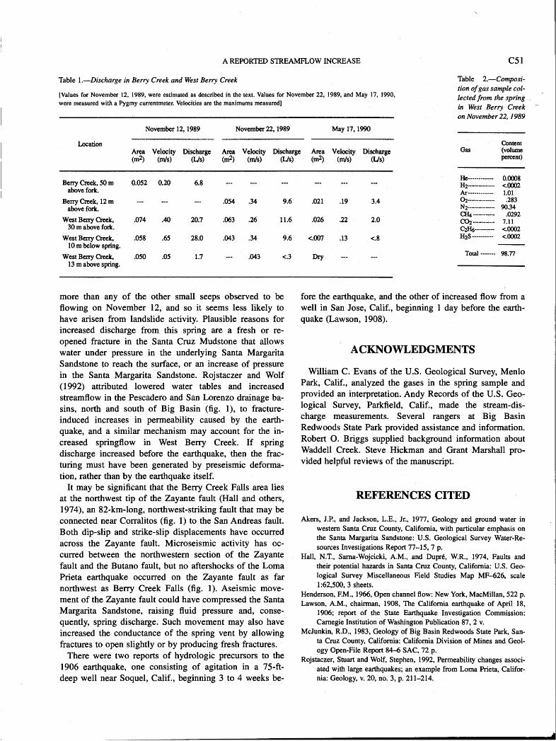
A REPORTED STREAMFLOW INCREASE c 5 1
Table 1.-Discharge in Berry Creek and West Berry Creek Table 2.-Composi- tion of gas sample col-
[Values for November 12, 1989, were estimated as described in the text. Values for November 22, 1989, and May 17, 1990, lected from the spring were measured with a Pygmy currentmeter. Velocities are the maximums measured] in West Berry Creek
November 12,1989 November 22,1989 May 17,1990
Location Area Velocity Discharge Area Velocity Discharge Area Velocity Discharge (m2) (ds) (Us) (m2) (ds) Us) (m2) (ds) (Us)
Berry Creek, 50 m 0.052 0.20 6.8 --- --- --- --- --- --- above fork.
Berry Creek, 12 m --- --- --- .054 .34 9.6 .021 .19 3.4 above fork.
WestBerryCreek, .074 .40 20.7 .063 .26 11.6 .026 .22 2.0 30 m above fork.
West Berry Creek, .058 .65 28.0 .043 .34 9.6 c.007 .13 <,8 10 m below spring.
West Berry Creek, .050 .05 1.7 --- .043 c.3 Dry --- --- 13 m above spring.
on November 22.1989
Content Gas (volume
percent)
more than any of the other small seeps observed to be flowing on November 12, and so it seems less likely to have arisen from landslide activity. Plausible reasons for increased discharge from this spring are a fresh or re- opened fracture in the Santa Cruz Mudstone that allows water under pressure in the underlying Santa Margarita Sandstone to reach the surface, or an increase of pressure in the Santa Margarita Sandstone. Rojstaczer and Wolf (1992) attributed lowered water tables and increased streamflow in the Pescadero and San Lorenzo drainage ba- sins, north and south of Big Basin (fig. I), to fracture- induced increases in permeability caused by the earth- quake, and a similar mechanism may account for the in- creased springflow in West Berry Creek. If spring discharge increased before the earthquake, then the frac- turing must have been generated by preseismic deforma- tion, rather than by the earthquake itself.
It may be significant that the Berry Creek Falls area lies at the northwest tip of the Zayante fault (Hall and others, 1974), an 82-km-long, northwest-striking fault that may be connected near Corralitos (fig. 1) to the San Andreas fault. Both dip-slip and strike-slip displacements have occurred across the Zayante fault. Microseismic activity has oc- curred between the northwestern section of the Zayante fault and the Butano fault, but no aftershocks of the Loma Prieta earthquake occurred on the Zayante fault as far northwest as Berry Creek Falls (fig. 1). Aseismic move- ment of the Zayante fault could have compressed the Santa Margarita Sandstone, raising fluid pressure and, conse- quently, spring discharge. Such movement may also have increased the conductance of the spring vent by allowing fractures to open slightly or by producing fresh fractures.
There were two reports of hydrologic precursors to the 1906 earthquake, one consisting of agitation in a 75-ft- deep well near Soquel, Calif., beginning 3 to 4 weeks be-
fore the earthquake, and the other of increased flow from a well in San Jose, Calif., beginning 1 day before the earth- quake (Lawson, 1908).
ACKNOWLEDGMENTS
William C. Evans of the U.S. Geological Survey, Men10 Park, Calif., analyzed the gases in the spring sample and provided an interpretation. Andy Records of the U.S. Geo- logical Survey, Parkfield, Calif., made the stream-dis- charge measurements. Several rangers at Big Basin Redwoods State Park provided assistance and information. Robert 0. Briggs supplied background information about Waddell Creek. Steve Hickman and Grant Marshall pro- vided helpful reviews of the manuscript.
REFERENCES CITED
Akers, J.P., and Jackson, L.E., Jr., 1977, Geology and ground water in western Santa Cruz County, California, with particular emphasis on the Santa Margarita Sandstone: U.S. Geological Survey Water-Re- sources Investigations Report 77-15, 7 p.
Hall, N.T., Sarna-Wojcicki, A.M., and Dupr6, W.R., 1974, Faults and their potential hazards in Santa Cruz County, California: U.S. Geo- logical Survey Miscellaneous Field Studies Map MF-626, scale 1:62,500,3 sheets.
Henderson, F.M., 1966, Open channel flow: New York, MacMillan, 522 p. Lawson, A.M., chairman, 1908, The California earthquake of April 18,
1906; report of the State Earthquake Investigation Commission: Carnegie Institution of Washington Publication 87, 2 v.
McJunkin, R.D., 1983, Geology of Big Basin Redwoods State Park, San- ta Cruz County, California: California Division of Mines and Geol- ogy Open-File Report 84-6 SAC, 72 p.
Rojstaczer, Stuart and Wolf, Stephen, 1992, Permeability changes associ- ated with large earthquakes; an example from Lorna Prieta, Califor- nia: Geology, v. 20, no. 3, p. 211-214.
THE LOMA PRIETA, CALIFORNIA, EARTHQUAKE OF OCTOBER 17,1989: EARTHQUAKE OCCURRENCE
PRESEISMIC OBSERVATIONS
NEAR-FIELD HIGH-RESOLUTION STRAIN MEASUREMENTS
CONTENTS
By Malcolm J.S. Johnston, U.S. Geological Survey; and
Alan T. Linde, Carnegie Institution of Washington
Page
C53 53 54 54 55 57 5 8 5 8
ABSTRACT
High-resolution strain recordings were made in deep boreholes throughout California before, during, and after the earthquake. The nearest dilatational strainmeters (sen- sitivity, 1 O-'O) and three-component tensor strainmeters (sensitivity, were 37 to 42 km, respectively, from the main-shock epicenter. High-quality data, including details of strain offsets, were recorded on both instruments through the earthquake. We have searched these data for indications of short-, intermediate-, and long-term strain redistribution and (or) fault slip that might have indicated imminent rupture. Short- and intermediate-term changes in both tensor strain and dilatational strain (not more than several nanostrain if any) during the minutes to months before the earthquake are at least 1,000 times smaller than that generated by the earthquake itself. If any short-term preseismic slip did occur at the nucleation point of the earthquake during the previous week, and if the type of slip was similar to that observed during the earthquake, its moment could be no more than dyne-cm. Stated an- other way, slip equivalent to that expected for an earth- quake with a magnitude of 5.3 could have occurred in the hypocentral region without the strainmeters detecting it at these distances and azimuthal positions. Longer-term changes in strain rate appear to have occurred in mid-1988 and mid-1989 at about the time of two ML=5 earthquakes in the hypocentral region on June 27, 1988, and August 8,
1989. Because regional strain redistribution in the epicen- tral area is not apparent in large-scale surface-displacement data over this region, these changes probably resulted from adjustment of nearby fault-slip rates at these times. Minor postseismic strain recovery (-14 percent) occurred in the month after the main shock.
INTRODUCTION
Although changes in the state of crustal stress and strain in the epicentral regions of moderate to large earthquakes have long been expected to precede the main shock (Mogi, 1985) and some intriguing indications of impending fault failure have been reported (for example, Kanamori and Cipar, 1974; Rikitake, 1976; Mogi, 1985; Linde and others, 1988), these signals have not been routinely observed. As instrumental sensitivity has increased and the effects of near-surface earth noise have been dramatically reduced (Sacks and others, 1971; Wyatt and others, 1982), quantifi- cation of "precursory" strain and tilt changes and identifi- cation of the underlying physics of failure have proved elusive (Johnston and others, 1987). Arrays of borehole in- struments have been installed in Japan (see summary by Mogi, 1981) and at several critical locations within the San Andreas fault system (Johnston and others, 1987) to inves- tigate these issues.
In expectation of a moderate to large earthquake in the Santa Cruz MountainsISan Juan Bautista section of the San Andreas fault, installation of an array of six deep-borehole dilatational strainmeters (Sacks and others, 1971) and two tensor strainmeters (Gladwin and others, 1987) was planned for this region in the early 1980's. However, only three of these eight instruments were actually installed (in 1982 and 1983), of which only two (one dilatometer and one tensor strainmeter) were operating at the time of the Loma Prieta earthquake (U.S. Geological Survey staff, 1990). High- resolution strain recordings were made on both of these in- struments through the time of the earthquake (Johnston and
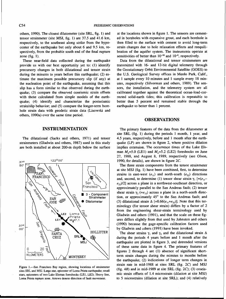
c54 PRESEISMIC OBSERVATIONS
others, 1990). The closest dilatometer (site SRL, fig. 1) and tensor strainmeter (site MSJ, fig. 1) are 37.5 and 41.6 km, respectively, to the southeast along strike from the hypo- center of the earthquake but only about 6 and 9.5 km, re- spectively, from the probable south end of the final rupture zone (fig. 1).
These near-field data collected during the earthquake provide us with our best opportunity yet to: (1) identify precursory changes in both dilatational and tensor strain during the minutes to years before this earthquake; (2) es- timate the maximum possible precursory slip (if any) at the nucleation point of the earthquake, assuming that this slip has a form similar to that observed during the earth- quake; (3) compare the observed coseismic strain offsets with those calculated from simple models of the earth- quake; (4) identify and characterize the postseismic strainJslip behavior; and (5) compare the longer-term bore- hole strain data with geodetic strain data (Lisowski and others, 1990a) over the same time period.
INSTRUMENTATION
The dilatational (Sacks and others, 1971) and tensor strainmeters (Gladwin and others, 1987) used in this study are both installed at about 200-m depth below the surface
Figure 1.-San Francisco Bay region, showing locations of strainmeter sites SRL and MSJ. Large star, epicenter of Lorna Prieta earthquake; small stars, epicenters of two Lake Elsman foreshocks (LEI, LE2). Heavy line, Loma Prieta rupture zone. Arrows denote direction of fault movement.
at the locations shown in figure 1. The sensors are cement- ed in boreholes with expansive grout, and each borehole is then filled to the surface with cement to avoid long-term strain changes due to hole relaxation effects and reequili- bration of the aquifer system. The instruments operate at sensitivities of better than 10-lo and respectively.
Data from the dilatational and tensor strainmeters are transmitted with 16- and 12-bit digital telemetry through the Geostationary Orbit Environmental Satellite (GOES) to the U.S. Geological Survey offices in Men10 Park, Calif., at 1 sample every 10 minutes and 1 sample every 18 min- utes, respectively (Silverman and others, 1989). The sen- sors, the installation, and the telemetry system are all calibrated together against the theoretical ocean-load-cor- rected solid-earth tides; this calibration is repeatable to better than 5 percent and remained stable through the earthquake to better than 1 percent.
OBSERVATIONS
The primary features of the data from the dilatometer at site SRL (fig. 1) during the periods 1 month, 1 year, and 4.5 years, respectively, before and 1 month after the earth- quake (LP) are shown in figure 2, where positive dilation implies extension. The occurrence times of the Lake Els- man ML=5.0 (LEI) and ML=5.2 (LE2) foreshocks on June 27, 1988, and August 8, 1989, respectively (see Olson, 1990, for details), are shown in figure 2C.
The three strain components from the tensor strainmeter at site MSJ (fig. 1) have been combined, first, to determine strains in east-west (ell) and north-south (eZ2) directions and, second, to determine (1) tensor shear strain y, [=(el e22)12] across a plane in a northwest-southeast direction, or approximately parallel to the San Andreas fault; (2) tensor shear strain y2 (=e12) across a plane in a north-south direc- tion, or approximately 45' to the San Andreas fault; and (3) dilatational strain A [=0.66(e,,+eZ2)]. Note that this ter- minology (for tensor shear strain) differs by a factor of 2 from the engineering shear-strain terminology used by Gladwin and others (1991), and that the scale on these fig- ures differs slightly from that used by Johnston and others (1990) because the gage-specific calibration factors used by Gladwin and others (1991) have been invoked.
The shear strains yl and y2 and the dilatational strain A during the periods 4 years before and 1 month after the earthquake are plotted in figure 3, and detrended versions of these same data in figure 4. The primary features of figures 2 through 4 are (1) absence of significant short- term strain changes during the minutes to months before the earthquake; (2) indications of longer term changes in strain rate in mid-1988 at sites SRL (fig. 2C) and MSJ (fig. 45) and in mid-1989 at site SRL (fig. 2 0 ; (3) coseis- mic strain offsets of 1.4 microstrain (dilation at site MSJ) to 5 microstrains (dilation at site SRL); and (4) relatively

NEAR-FIELD HIGH-RESOLUTION STRAIN MEASUREMENTS c55
minor postseismic strain recovery (- 14 percent) in the month after the earthquake, evident in all the strain data.
An expanded-scale plot of dilatational strain during the week before the earthquake (fig. 5A) shows more detail of the short-term strain immediately before the earthquake, and the same data with earth tides and atmospheric-load- ing effects removed are plotted in figure 55. The 95-per- cent-confidence limits of these data are 1.1 nanostrain. Thus, if short-term precursory strain changes occurred during the week before the earthquake, they could not have been more than a nanostrain or so. Similarly, during the month before the earthquake, precursory strain excur- sions could not have been more than about 5 nanostrain.
DISCUSSION
An important issue concerns the amount of precursory slip that might have occurred in the hypocentral region be- fore the earthquake. If we make the reasonable assumption that, if preseismic slip did occur, it had the same rupture mechanism as the subsequent earthquake, we can estimate the maximum precursory slip moment M generating strains of less than 1 nanostrain at the two strainmeter
sites during the minutes to weeks before the earthquake. Thus, taking the geodetically determined source mecha- nism (Lisowski and others, 1990a) and the seismically de- termined depth (Dietz and Ellsworth, 1990) of the earthquake to indicate precursory source type and location, and using Okada's (1985) dislocation-model formulation, we obtain dyne-cm. Using Aki's (1987) magnitu- delmoment relation, the largest allowable precursory slip moment at the earthquake source is equivalent to an earth- quake of M=5.3.
We are less certain about our measurements of strain- rate changes at periods of years or longer. Long-term changes in the geodetic lines were initially reported as a precursor to the earthquake by Lisowski and others (1990b). However, these changes have since been shown not to be significant (Lisowski and others, 1992). Never- theless, we have checked our borehole strainmeter data during the same period and note that strain-rate changes did occur in mid-1988 (shown for dilatometer data in fig. 2C and detrended fault-parallel shear strain y, in fig. 45). These changes correspond approximately to the time of the first Lake Elsman foreshock (LEI), as shown in figures 2C and 45. A less significant change in long-term strain rate occurred in mid-1989 at about the time of the second
TIME
Figure 2.-Dilatational strain recorded at site SRL (fig. 1) 1 month before and 1 month after (A), 1 year before and 1 month after (B), and 4.5 years before and 1 month after (Q Loma Prieta earthquake. Arrows denote occurrence times of Lake Elsman ML=5.0 (LEI) and ML=5.2 (LE2) foreshocks of June 27, 1988, and August 8, 1989, respectively, and of Loma Prieta earthquake (LP).

PRESEISMIC OBSERVATIONS
20 I
TIME (years)
Figure 3.-Tensor shear strains y , (A) and y2 (B) and dilatational strain ( 0 derived from tensor-strain data at site MSJ (fig. 1) 4 years before and 1 month after Loma Prieta earthquake. Arrows denote occurrence times of Lake Elsman ML=5.0 (LEI) and ML=5.2 (LE2) foreshocks of June 27, 1988, and August 8, 1989, respectively, and of Loma Prieta earthquake (LP).
TIME (years)
Figure 4.-Residuals of tensor shear strains y , (A) and y2 (B) and dilatational strain (Q plotted in figure 3, after removal of exponential functions determined by least-squares analysis. Exponentials result from curing of grout used to emplace instruments and from recovery of borehole stresses relieved during drilling, not from tectonic processes.

NEAR-FIELD HIGH-RESOLUTION STRAIN MEASUREMENTS c57
Lake Elsman foreshock on August 8, 1989 (fig. 2C). With so few data, however, it is difficult to place much signifi- cance on these long-term strain changes.
Although the measurements of coseismic strain offsets are too few to determine the source parameters of the earthquake, we can compare the observed offsets with those calculated from a best-fit static model of the earth- quake constrained by inversion of the surface geodetic data (Lisowski and others, 1990a). This comparison can be made by modeling the source as rectangular fault planes with uniform slip, using Okada's (1985) formulation for surface deformations due to a dislocation embedded in an elastic half-space. The calculated strain values at sites SRL and MSJ are quite sensitive to the details of complex fault geometry at the south end of the rupture zone (fig. I), although this geometry is poorly constrained by the large-scale geodetic data (Lisowski and others, 1990a) at this stage of analysis. Until a better fault-slip model for the south end of the Loma Prieta rupture zone is obtained, we cannot easily compare the observed and calculated strain offsets at sites SRL and MSJ.
The simplest interpretation of the immediate postseismic strain data is in terms of rebound following slight over- shoot of the fault rupture. Such an interpretation, however, is probably too simple because the geometry of fault rup- ture near and beneath these instruments is still changing, as indicated by continuing seismicity (aftershocks) and
varying surface displacements throughout this region (Lisowski and others, 1990a).
CONCLUSIONS
Short-term precursory strain changes are not apparent in the data from a dilatational strainmeter (located 37.5 krn downstrike from the main-shock epicenter) and a tensor strainmeter (located 41.6 km from the main-shock epicen- ter). If precursory strains actually occurred, they are less than 0.1 percent of the strain offset generated on these in- struments by the earthquake. These observations constrain the preseismic moment release at the nucleation point of the earthquake to less than dyne-cm. In other words, any aseismic slip in the hypocentral region greater than that which commonly occurs during an M=5.3 earthquake would have been detected on the strainmeters at these dis- tances and azimuthal positions. Using Kanamori and Anderson's (1975) relations between magnitude and source size for an M=5.3 earthquake, the amount of slip that might have occurred on a 7- by 7-km patch at the hypocen- ter could not have been more than about 7 cm. Though better positioned over the hypocentral region, geodetic measurements also would not detect this amount of fault slip by inversion of surface-displacement data because of poorer resolution (-1 cm in horizontal-displacement meas- urements; Lisowski and others, 1990a).
October 1989
Figure 5.-Dilatational strain. A, Data during week before Loma Prieta earthquake (LP). B, Same data at an expanded scale, with earth-tidal and atmospheric-loading effects removed.

C58 PRESEISMIC OBSERVATIONS
Long-term strain changes, such as might be expected from strain redistribution in the epicentral region, occurred in mid-1988 and mid-1989, at about the time of the two ML=5 Lake Elsman fores hocks in the h ypocen tral region on June 27, 1988, and August 8, 1989. However, because these changes are not clearly observed on geodetic lines over this area, they most likely resulted from more local changes in the spatial pattern of fault slip and are not re- lated directly to the Loma Prieta source region, or from larger scale regional strain, as proposed by Gladwin and others (1991). A more complete array of instruments was clearly needed around the epicenter of this earthquake to resolve this long-term-strain issue and such other issues as determination of the best coseismic-slip models and the details of postseismic-slip growth and geometry.
ACKNOWLEDGMENTS
We thank M.T. Gladwin for tensor strain data and Doug Myren for careful maintenance of the instruments.
REFERENCES CITED
Aki, Keiiti, 1987, Magnitude-frequency relation for small earthquakes; a clue to the origin of fm of large earthquakes: Journal of Geophysi- cal Research, v. 92, no. B2, p. 1349-1355.
Dietz, L.D., and Ellsworth, W.L., 1990, The October 17, 1989, Loma Prieta, California, earthquake and its aftershocks; geometry of the sequence from high-resolution locations: Geophysical Research Let- ters, v. 17, no. 9, p. 1417-1420.
Gladwin, M.T., Gwyther, R.L., Hart, R.H.G., Francis, M.F., and Johnston, M.J.S., 1987, Borehole tensor strain measurements in Cal- ifornia: Journal of Geophysical Research, v. 92, no. B8, p. 7981- 7988.
Gladwin, M.T., Gwyther, R.L., Higbie, J.W., and Hart, R.H.G,, 1991, A medium term precursor to the Loma Prieta earthquake?: Geophysi- cal Research Letters, v. 18, no. 8, p. 1377-1380.
Johnston, M.J.S., Linde, A.T., and Gladwin, M.T., 1990, Near-field high resolution strain measurements prior to the October 18, 1989, Loma Prieta Me 7.1 earthquake: Geophysical Research Letters, v. 17, no. 10, p. 1777-1780.
Johnston, M.J.S., Linde, A.T., Gladwin, M.T., and Borcherdt, R.D., 1987, Fault failure with moderate earthquakes: Tectonophysics, v. 144, no. 1-3, p. 189-206.
Kanamori, Hiroo, and Anderson, D.L., 1975, Theoretical basis of some empirical relations in seismology: Seismological Society of America Bulletin, v. 65, no. 5, p. 1073-1096.
Kanamori, Hiroo, and Cipar, J.J., 1974, Focal processes of the great Chil- ean earthquake, May 22, 1966: Physics of the Earth and Planetary Interiors, v. 9, p. 128-136.
Linde, A.T., Suyehiro, Kiyoshi, Miura, Satoshi, Sacks, I.S., and Takagi, Akio, 1988, Episodic aseismic earthquake precursors: Nature, v. 334, no. 6182, p. 513-515.
Lisowski, Michael, Prescott, W.H., Savage, J.C., and Johnston, M.J.S., 1990a, Geodetic estimate of coseismic slip during the 1989 Loma Prieta, California, earthquake: Geophysical Research Letters, v. 17, no. 9, p. 1437-1440.
Lisowski, Michael, Prescott, W.H., Savage, J.C., and Svarc, J.L., 1990b, A possible geodetic anomaly observed prior to the Loma Prieta earthquake: Geophysical Research Letters, v. 17, no. 8, p. 1211- 1214.
Mogi, Kiyoo, 1981, Earthquake prediction program in Japan, in Simpson, D.W., and Richards, P.G., eds., Earthquake prediction; an interna- tional review: Washington, D.C., American Geophysical Union, p. 635-666.
1985, Earthquake prediction: Tokyo, Academic Press, 355 p. Okada, Yoshimitsu, 1985, Surface deformation due to shear and tensile
faults in a half-space: Seismological Society of America Bulletin, v. 75, no. 4, p. 1135-1154.
Olson, J.A., 1990, Seismicity in the twenty years preceding the Loma Prieta, California earthquake: Geophysical Research Letters, v. 17, no. 9, p. 1429-1432.
Rikitake, Tsuneji, 1976, Earthquake prediction: Amsterdam, Elsevier, 357 p.
Sacks, I.S., Suyehiro, Shigeji, Evertson, D.W., and Yamagishi, Yoshiaki, 1971, Sacks-Evertson strainmeter, its installation in Japan and some preliminary results concerning strain steps: Papers in Meteorology and Geophysics, v. 22, p. 195-207.
Silverman, Stan, Mortensen, C.E., and Johnston, M.J.S., 1989, A satel- lite-based digital data system for low-frequency geophysical data: Seismological Society of America Bulletin, v. 79, no. 1, p. 189-198.
U.S. Geological Survey staff, 1990, The Loma Prieta, California, earth- quake; an anticipated event: Science, v. 247, no. 4940, p. 286-293.
Wyatt, F.K., 1988, Measurements of coseismic deformation in southern California; 1972-1982: Journal of Geophysical Research, v. 93, no. B7, p. 7923-7942.
Wyatt, F.K., Beckstrom, Kent, and Berger, Jon, 1982, The optical an- chor-a geophysical strainmeter: Seismological Society of America Bulletin, v. 72, no. 5, p. 1707-1715.

THE LOMA PRIETA, CALIFORNIA, EARTHQUAKE OF OCTOBER 17,1989: EARTHQUAKE OCCURRENCE
PRESEISMIC OBSERVATIONS
A SHEAR-STRAIN PRECURSOR
By Michael T. Gladwin, Ross L. Gwyther, and Rhodes H.G. Hart, University of Queensland, Australia
CONTENTS
ABSTRACT
The earthquake provided unique near-field borehole tensor strain observations. Medium-term data from a strainmeter installed at San Juan Bautista, Calif., showed a clear anomalous change in fault-parallel shear strain rate beginning about 1 year before the earthquake. The anoma- ly ultimately reached 30 percent of the coseismic offset. The signal resembles some of the changes in strain rates reported from the geodetic record and nearby creep anom- alies, suggesting a broad regional anomaly. The limited spatial sampling available, however, prevents determina- tion of a causal link useful for prediction between these data and the earthquake.
INTRODUCTION
Measurements of earth strain within several source di- mensions of an earthquake in the years before the event should yield information about the processes of strain ac- cumulation and concentration leading to failure, and may contribute to specific prediction of earthquakes.
Because the expected strain rates are about 1 micro- straidyr or less, strain data are potentially contaminated by spurious signals from ground-coupling problems and nontectonic effects from thermal, ground-water, or cultural sources (Agnew, 1986). Early near-surface point measure- ments provided little useful insight. Significant improve- ments in signal quality and stability, however, have been achieved with the deployment of borehole strainmeters at
depths of about 200 m. Quality borehole strain data have been obtained at such depths in Japan for nearly 20 years (Sacks and others, 1971). Instruments provide almost con- tinuous data at sensitivities more than 1,000 times greater than those of quality geodetic networks and, depending on the borehole depth and the complexity of local geology, operate in a relatively noise free environment. Limitations on the data focus on the representativeness of the small sample of rock surrounding the instrument, and on the reli- ability of the coupling of the instrument to the rock mass; measurements indicate that performance is not limited by the intrinsic sensitivity or stability of the instrument pack- age itself (Agnew, 1986; Gladwin and others, 1987). The borehole tensor strainmeter used here (Gladwin, 1984) measures both hydrostatic and shear strain in the ground with subnanostrain resolution and a long-term stability bet- ter than 100 nanostraidyr (Gladwin and others, 1987). These stability figures are also evident in the present data.
Two borehole instruments (a Sacks-Evertson dilatometer and a Gladwin tensor strainmeter) were operating in the region of the San Andreas fault at the time of the earth- quake. High-resolution recordings were made on each of these instruments before, during, and after the earthquake (Johnston and others, 1990). The tensor strainmeter in- stalled at San Juan Bautista, Calif., was located 40 km southeast of the epicenter and within about 10 km of the southward extent of the rupture zone (fig. 1). The data ob- tained during the 4-year period before the earthquake pro- vide a rare opportunity to observe local strain processes before a large earthquake. Data from the 2-year period after the earthquake also show significant signals, as dis- cussed in other chapters of this report.
DATA AND PROCESSING
The San Juan Bautista strainmeter was installed in late Sep- tember 1983 at a depth of 150 m, using an expansive grout. Day averages for the three components of the strainmeter are plotted in figure 2. Immediate postinstallation observations are dominated by grout compression of the instrument and by thermally controlled decay as the instrument site reestablished

C60 PRESEISMIC OBSERVATIONS
equilibrium with its surroundings. The installation was im- mediately after drilling, and so this grout curing was then followed by an exponential recovery of the virgin stress field relieved during the drilling process.
Exponential signals are irrelevant to the monitoring of strain changes that may be occurring in the region, and so
Figure 1.-Loma Prieta region, Calif., showing locations of major faults (solid lines), geodetic stations (triangles), and borehole strainmeter sites (squares): SJT, Gladwin tensor strainmeter; SRL, Sacks-Evertson dilatometer. Heavy line, Loma Priet. rupture zone; dashed lines, relevant geodetic lines; stars, epicenters of main shock (large) and two Lake Els- man foreshocks (small),
they were removed from the raw data by a least-squares analysis to produce the residual component data used in subsequent strain analysis. Residuals for the three gauge components from July 1986 are plotted in figure 3; no smoothing has been applied.
The residuals thus produced are sensitive to details of the exponential removal procedure. To obtain meaningful residuals in the present context of a search for possible precursory signals, regions of data that are contaminated by obvious nonexponential processes or are themselves in- volved in the time window of the precursors to be identi- fied must be excluded from the analysis. Disturbances of the record associated with the Morgan Hill, Calif., earth- quake of April 24, 1984, and experiments at the site result- ing in large transients due to downhole heating necessitated exclusion of the data from April 1984 to mid- 1986. All the data after March 1988, which might relate to the change in gradient evident on the raw records, were also excluded. The same regions were excluded for all components.
A wide range of data windows were investigated to veri- fy that the strain-rate change was not an artifact of the detrending procedure. The onset and characteristics of the linear-strain-rate anomaly was always evident even if the window was extended into 1989. The exponentials deter- mined are plotted (offset for better visibility) in figure 2. These exponential processes are to be expected from all standard rheologic models. The remarkable flatness of the residuals before mid-1988 indicates that the determined exponentials adequately describe the long-term recovery
Figure 2.-Three-component raw strain data from San Juan Bautista strainmeter site. Measurements are sim- ple day averages expressed in nominal microstrain measured within instrument. Fitted exponentials are also shown, offset for clarity. Instrument was nonoperational for several months in 1987.

A SHEAR-STRAIN PRECURSOR C6 1
of the hole. The measured grout-curing exponential time constants range from about 90 to 110 days, and the hole- recovery exponentials from about 800 to 1,000 days.
These residuals are combined to produce shear and areal strains, which are scaled by hole-coupling parameters to account for the areal- and shear-strain response of the in- strument inclusion (Gladwin and Hart, 1985). These pa- rameters are determined by a calibration procedure involving, for each gage, a comparison of individual tidal components of the theoretical earth-tidal strains (corrected for ocean loading) with tidal components of the strains ob- served on the instrument. The procedure by which individ- ual channels are tidally calibrated is described in detail by Hart and others (in press).
The resulting areal- and shear-strain records are plotted in figure 4. These records completely specify the strain field in the horizontal plane defined with the x-axis east and the y-axis north, where yl and y2 are shears with the maximum shear across northwest-southeast or northeast- southwest aad north-south or east-west planes, respective- ly; they are related to the tensor strain components e,, by the relations ea=em+eyy, yl=en-eyy, and y2=2ey. The con- vention of extension positive is used. To facilitate compar- ison of our data with geodetic records in the region, we have chosen to use engineering strains here rather than the tensor definitions used in our previous publications. For areal strain, we use the symbol ea rather than A (areal dila- tation) of Prescott and others (1979), because A commonly refers to volumetric dilatation. No other processing or fil-
tering has been applied to these records. The data show a negligible response to rainfall, and we have conducted no hydrologic studies of the region.
DISCUSSION
The coseismic areal-strain step seen in figure 4 is +2,140 nanostrain, yl=+l,840 nanostrain, and y2=-3,790 nano- strain. Strain axes on this figure differ from those previ- ously reported by Johnston and others (1990), which were in non-engineering units and were derived without the gage-specific calibration procedure used here. As noted by Johnston and others (1990), dislocation models based on large-scale geodetic data appear to be inappropriate for the southeast end of the rupture zone and do not at this stage predict the coseismic areal-strain steps for both Searle Road and San Juan Bautista, which recorded comparable expansions. No short-term (seconds to days) precursory signals are evident in the records (Johnston and others, 1990).
Apart from the coseisrnic step, these records are notable for their overall stability. The areal strain, for example, is constant at the 50-nanostrain level from 1986 to early 1989. Investigation of the instrumental response to the At2 and 0, tidal components indicates that coupling conditions have not changed significantly since 1986.
The most significant feature in the records is the onset of a strain-rate change in y, strain clearly identifiable over
Gage 3
Figure 3.-Three-component residuals of strain data from San Juan Bautista strainmeter after removal of exponentials; data after March 1988 were excluded from fit. Change of slope evident on all components represents nearly 20 percent of coseismic amplitude for gage 3, 25 percent for gage 2, and less than 10 percent for gage 1. LEI and LE2, times of two Lake Elsman foreshocks; LP, time of Loma Prieta main shock.

C62 PRESEISMIC OBSERVATIONS
3 months in late 1988. A steady additional strain-rate change of 1,140 nanostrainlyr was established, ultimately accumulating more than 30 percent of the coseismic step. Because the ea component is essentially constant, this change in the strain field is predominantly a shear. Fur- thermore, y , is the dominant shear, and so the maximum shear is approximately parallel to the San Andreas fault (striking N. 50' W. here), consistent with increased shear stress across the fault in the direction of subsequent fail- ure. The data imply a strain-rate change of approximately 370 nanostrain of compression per year for the e compo- nent and, during the early part of 1989, of approximately 570 nanostrain of extension for the eu component.
In fact, this anomaly ceased immediately after the earth- quake, and a new and higher rate of fault-parallel shear accumulation was established about 4 months later and has
continued for at least 18 months. These data (Gwyther and others, 1992) are discussed in other chapters of this report.
The power spectrum for the 3 years of areal-strain data plotted in figure 5 provides a reasonable estimate of the lowest anomalous signal detectable within any period range. Integration of the spectrum over the period band above 3 months indicates a standard deviation of approxi- mately 20 nanostrain for assumed-stationary data. This same standard deviation would be produced by a single 3- month-duration ramp excursion of 100-nanostrain ampli- tude at an arbitrary point in our 34-month record. A signal excursion similar to our anomaly can thus be identified as anomalous if it exceeds approximately 100 nanostrain in 3 months. By this criterion, the y, strain record was identifi- ably anomalous by November 1988, almost a year before the earthquake (fig. 6).
...................... ....................... ........................ ....................... c .u g -1000
8 ....................... g -2000
2 LEI LE2 LP
Figure 4.-Reduced areal and shear strains derived from residuals in figure 3. A, Areal strain. B, y l strain. C, y2 strain. Data have been calibrated and corrected for borehole amplification effects. LEI and LE2, times of two Lake Elsman foreshocks; LP, time of Loma Prieta main shock.

A SHEAR-STRAIN PRECURSOR C63
As shown in figure 1, the area to the north of the epicen- Elsman "foreshock." The least-squares-determined change ter is covered by a geodetic network of three lines radiating in gradient of the Allison line (-15.1+/-2.6 rnmlyr) appears from Lorna Prieta to Allison, Mount Hamilton, and Eagle to be better defined than for the Hamilton line (-8.1+/-2.2 Rock (Lisowski and others, 1990a, b). Lisowski and others mrnlyr). Lower rates are suggested by Global Positioning reported a marginally significant change in gradient for the Satellite (GPS) data for the Allison line. The dominant ef- Allison and Mount Hamilton lines after the June 1988 Lake fect is on the Allison line, which runs nearly north-south
year I
month week
Frequency (Hz)
Figure 5.-Power spectrum for 1,024 days of areal-strain data beginning approximately 1986.5.
1 LEI LE2 LP 1
Figure 6.-Areal- and shear-strain data for 3%-year period before Lorna Prieta earthquake. LEI and LE2, times of two Lake Elsman foreshocks; LP, time of Loma Prieta main shock.

C64 PRESEISMIC OBSERVATIONS
and measures the integral of the eyy component along its length. Geodetic data show an increased compressional rate through 1989 equivalent to 300 nanostrainlyr averaged over the line, comparable to the borehole measurement. The Mount Hamilton data indicate an average compressional strain rate of approximately 250 nanostrainlyr, in compari- son with the implied value of 180 nanostrainlyr from bore- hole data for the period mid-1988 to March 1989.
As noted above, our data imply an extension of 570 nanostrain in the en component, which would be expected to show on the Loma Prieta-to-Eagle Rock line. No such extension is evident, however, in the geodetic data for this interval, although the GPS data appear to indicate an ex- tension possibly as large as 650 nanostrainlyr over the same interval.
The similarity in the timing and possible magnitude of the borehole data to the change of gradient in mid-1988 of the geodetic measurements may be only coincidental. However there is also some indication of a regional creep anomaly during the 2-year period before the earthquake in the data from several creepmeters within 20 km of San Juan Bautista (Gwyther and others, 1992). Burford (1988) noted creep retardation before moderate earthquakes in ad- jacent regions. These creep data provide further support for a regional preearthquake strain anomaly, at least in the San Juan Bautista area, independent of the geodetic data.
Although other models are not excluded, the data could imply a regional increase in shear-strain rate acting to in- crease shear stress across the fault in the direction of failure approximately 1 year before the earthquake. This increase is remarkably linear and shows no evidence of accelerating failure. With such sparse coverage of the region, however, the temptation to identify this anomaly as a precursor must be resisted.
CONCLUSIONS
A well-established change in shear-strain rate was ob- served at the San Juan Bautista tensor strainmeter site al- most a year before the earthquake, with an ultimate amplitude of more than 30 percent of the final coseismic event. Together with geodetic data, this observation may indicate a regional loading of the fault in a direction con- sistent with final failure. No causal link to the event can be established, however, because of inadequate spatial sampling.
Although the anomaly may have been caused by a source in the immediate vicinity of the instrument, the similarity in amplitude, sense of shear, and time signature to the geodetic observations argue for a regional strain dis- turbance. Anomalous strain changes reported at the Searle Road dilatometer (Johnston and others, 1990) may also confirm this conclusion, although no compatible areal- strain effects are evident in our data.
The characteristics of the anomaly are not well de- scribed by any current theoretical precursor modeling studies, which predict short-term tertiary-creep phenome- na. This anomaly is better described as indicating a proc- ess of regional stress concentration caused by a localized departure from the regional tectonic strain rates as deter- mined by geodetic studies. A similar anomaly was report- ed (Wyss and others, 1990) for the active section of the San Andreas fault at Parkfield, Calif.
Immediately after the earthquake, the strain rate returned for about 10 days to its value before the anomaly (that is, mid-1988), then decreased for 2 months. By May 1990, after the Chittenden, Calif., aftershock sequence, a new and higher rate of shear strain accumulation had been es- tablished. These data, together with associated creep anomalies, are discussed in other chapters of this report.
As a case study, this observation strongly underlines the need to deploy adequate-size arrays of strain instruments, the importance of measuring the total strain field at each site rather than single components, and the importance and interdependence of short-baseline, high-resolution data and the absolute long-baseline data provided in this case by the geodetic array. Our results demonstrate that minimal processing of borehole data to remove borehole-equilibra- tion processes produces residuals with a stability adequate for short- to intermediate-term tectonic monitoring rele- vant to precursor studies. In this context, the observations reported here are the only objective pointer to performance expectations for a future array of borehole strainmeters.
ACKNOWLEDGMENTS
This research was supported by U.S. Geological Survey grants 14-08-0001 4 1 190 and 14-08-0001-G1376. The instruments were previously developed under awards from the Australian Research Grants Scheme and fabricated by R. Willoughby and staff in house. We thank J. Healy, M. Francis, R. Mueller, and R. Liechti for installation and maintenance support, K. Breckenridge for data retrieval, and A.T. Linde and M.J.S. Johnston for their extensive support and cooperation in the program.
REFERENCES CITED
Agnew, D.C., 1986, Strainmeters and tiltmeters: Reviews of Geophysics, v. 24, no. 3, p. 579-624.
Burford, R.O., 1988, Retardations in fault creep rates before local moder- ate earthquakes along the San Andreas fault system, central Califor- nia: Pure and Applied Geophysics, v. 120, no. 2-4, p. 499-529.
Gladwin, M.T.,1984, High precision multi component borehole deforma- tion monitoring: Reviews of Scientific Instruments, v. 55, p. 2011- 2016.
Gladwin, M.T., Gwyther, R.L., Hart, R.H.G., Francis, M.F., and Johnston, M.J.S., 1987, Borehole tensor strain measurements in California: Journal of Geophysical Research, v. 92, no. B8, p. 7981-7988.

A SHEAR-STRAIN PRECURSOR C65
Gladwin, M.T., and Hart, R.H.G., 1985, Design parameters for borehole strain instrumentation: Pure and Applied Geophysics, v. 123, p. 59- 88.
Gwyther, R.L., Gladwin, M.T., and Hart, R.H.G., 1992, A shear strain anomaly following the Loma Prieta earthquake: Nature, v. 356, no. 6365, p. 142-144.
Hart, R.H.G., Wyatt, F.K., Agnew, D.C., Gwyther, R.L., and Gladwin, M.T., in press, Tidal calibration of borehole strain instruments: Jour- nal of Geophysical Research.
Johnston, M.J.S., Linde, A.T., and Gladwin, M.T., 1990, Near-field high resolution strain measurements prior to the October 18, 1989, Loma Prieta Me 7.1 earthquake: Geophysical Research Letters, v. 17, no. 10, p. 1777-1780.
Lisowski, Michael, Prescott, W.H., Savage, J.C., and Johnston, M.J.S.,
1990a, Geodetic estimate of coseismic slip during the 1989 Loma Prieta, California, earthquake: Geophysical Research Letters, v. 17, no. 9, p. 1437-1440.
Lisowski, Michael, Prescott, W.H., Savage, J.C., and Svarc, J.L., 1990b, A possible geodetic anomaly observed prior to the Loma Prieta earthquake: Geophysical Research Letters, v. 17, no. 8, p. 1211- 1214.
Sacks, I. S., Suyehiro, Shigeji, Evertson, D.W., and Yamagishi, Yoshiaki, 1971, Sacks-Evertson strainmeter, its installation in Japan and some preliminary results concerning strain steps: papers in Meteorology and Geophysics, v. 22, p. 195-207.
Wyss, Max, Slater, L.E., and Burford, R.O., 1990, Decrease in deforma- tion rate as a possible precursor to the next Parkfield earthquake: Nature, v. 345, no. 6274, p. 428-431.

THE LOMA PRIETA, CALIFORNIA, EARTHQUAKE OF OCTOBER 17,1989: EARTHQUAKE OCCURRENCE
PRESEISMIC OBSERVATIONS
NO CONVINCING PRECURSORY GEODETIC ANOMALY OBSERVED
By Michael Lisowski, James C. Savage, William H. Prescott, Jerry L. Svarc, and Mark H. Murray, U.S. Geological Survey
CONTENTS
ABSTRACT
Monthly Geodolite measurements since mid- 198 1 of the distances from a geodetic station located 11 km from the epicenter of the Loma Prieta earthquake to three stations 30 to 40 km distant provide an unusually complete record of deformation in the epicentral region during the years before the earthquake. The rate of change in line length for the only line crossing the eventual rupture zone is con- stant during this entire interval. About 1.3 years before the earthquake, at about the time of the first Me5 foreshock, the rate of change in line length for the other two lines appears to increase. Other similar, though smaller, differ- ences in this rate are apparent in the 8-year record. How- ever, no increase in the deformation rate before the earthquake is apparent in measurements of the same lines made with the Global Positioning System. Thus, there does not appear to have been a geodetically detectable strain precursor to the earthquake.
INTRODUCTION
The earthquake ruptured a section of the San Andreas fault along which crustal deformation had been monitored since August 198 1. The monitoring consisted of frequent (approx- imately monthly) measurements of the distance from geo- detic station Loma Prieta (fig. 1) at the summit of the Santa Cruz Mountains to geodetic stations on three nearby moun- tains: Allison (43 km distant), Eagle Rock (31 km distant), and Mount Hamilton (3 1 km distant). Approximately annual
measurements of the distance from Loma Prieta to Eagle Rock and Mount Hamilton extend back to 1972. Line lengths are measured with a Geodolite, a precise electro-optical dis- tance-measuring instrument, and the refractivity correction is determined from meteorologic profiles measured from a small airplane flying along the line at the time of ranging (Savage and Prescott, 1973). The precision (lo) of measure- ment is about 9 mm for the line to Allison and about 7 mm for the lines to Eagle Rock and Mount Hamilton.
In addition to Geodolite measurements, Global Position- ing System (GPS, a radio-interferometric technique of de- termining relative position) measurements of the same lines were made approximately monthly since mid-1987 (Davis and others, 1989). The purpose of those measurements was to test the precision of the GPS measurements against the standard of the Geodolite measurements. The GPS measure- ments provide an independent determination of the distance between mountaintops and a unique determination of rela- tive horizontal- and vertical-position change.
A general description of the earthquake was given by the U.S. Geological Survey staff (1990). The epicenter is about 11 km southwest of geodetic station Loma Prieta (fig. I), and the focal depth is 17 km (Dietz and Ellsworth, 1990). The earthquake was caused by oblique slip on a 37-km- long segment of the San Andreas fault. The rupture plane dipped about 70' SW. A preliminary estimate of the slip on the fault is 1.6±0. m of right-lateral slip and 1.2±0. m of reverse slip in the depth interval 5-18 km (Lisowski and others, 1990). Geodetic station Loma Prieta is located 3.5 km from the San Andreas fault and approximately midway between the ends of the rupture zone.
The main shock was preceded by two M-5 earthquakes, which in retrospect have been identified as foreshocks. The earlier foreshock occurred at 14-km depth on June 27, 1988, and the later at 17-km depth on August 8, 1989. The June 27, 1988, foreshock was called the Lake Elsman earthquake by Oppenheimer and others (1990). The loca- tions of the epicenters of these foreshocks are shown in figure 1. The two foreshocks are about 10 km distant from the main shock.

C68 PRESEISMIC OBSERVATIONS
GEODOLITE MEASUREMENTS three different stations on Loma Prieta: Loma USE (1972- 1982.9), Loma DWR (1982.9-1984.8), and Loma NCER
The distances measured by Geodolite from Loma Prieta (1984.8 onward). The distances from station Loma DWR to Allison, Eagle Rock, and Mount Hamilton as a function are corrected for eccentricity to station Loma USE, the of time are shown in figure 2. Monitoring began in early original station. Station Loma DWR was used temporarily September 1981, and the last measurements shown were to monitor some additional lines not visible from station made on October 3, 1989, just 2 weeks before the earth- Loma USE. In 1983, the tablet at station Loma USE was quake. During the first year, measurements were made ap- vandalized, and a tablet stamped "Loma NCER was set in proximately biweekly, but subsequently they were made the same drill hole. No eccentric correction was applied to more nearly monthly. The shaded bands in figure 2 repre- the measurements from station Loma NCER, and no off- sent a smoothed version of the data, with each band lo sets in distance are obvious at the time when measure- wide. (The precise smoothing routine used is unimportant ments began from station Loma DWR or Loma NCER. because the smoothed curves are intended only as aids in The times of nearby Ma5 earthquakes are marked with visualizing trends in the data.) Measurements were made at solid vertical lines in figure 2. The Morgan Hill earth-
Figure 1.-Loma Prieta, Calif., region, showing locations of epicenters of main shock and two foreshocks (numbered stars): 1, June 27, 1988, Lake Elsman foreshock; 2, August 8, 1989, Lake Elsman foreshock; 3, October 17, 1989, main shock. Unnumbered stars, epicenters of Morgan Hill, Mount Lewis, and Alum Rock earthquakes; triangles, geodetic stations. Heavy lines show extent of ruptures as indicated by aftershocks. MSJ, Gladwin tensor strainmeter; SRL, Sacks-Evertson dilatometer.

NO CONVINCING PRECURSORY GEODETIC ANOMALY OBSERVED C69
quake (ML=6.2; Bakun and others, 1984), which occurred on April 24, 1984, near Mount Hamilton (fig. I), produced a coseismic offset in the line to Mount Hamilton. No off- sets are apparent at the time of the Mount Lewis (M=5.7; Oppenheimer and others, 1990) or Alum Rock (M=5.1; Oppenheimer and others, 1990) earthquakes (see fig. 1 for locations of epicenters). There appears to be a change in the trend of the line-length data for two of the lines (to Allison and Mount Hamilton) in mid-1988, at about the time of the first of the two Loma Prieta foreshocks; how- ever, no such change is obvious in the Eagle Rock data. Similar, though less significant, increases in the rate of line-length change also occur for the same two lines in mid-1986, after the Mount Lewis earthquake, and about 1.2 years before the Morgan Hill earthquake (1984.3). We conclude that the change in the trend observed in mid- 1988 in the lines to Allison and Mount Hamilton is only the most conspicuous of several similar changes evident in the 8-year record plotted in figure 2.
To judge the significance of this change in trend, we compare the rates of line-length change (dLldt) before and after the June 27, 1988, foreshock. We take the occurrence of this foreshock as an indication that the failure process is already underway; thus, it furnishes an independent criteri- on for dividing the data. The trends of the data before and after the foreshock are estimated from the slope of linear fits to the data. Estimated rates of line-length change for all the data before the foreshock (except for the line to Mount Hamilton, which is offset by the Morgan Hill earthquake) and for the subset of the data from station Loma NCER (late 1984) are listed in table 1. Only the change of slope in the line to Allison for the shorter inter- val before the foreshock (second line, table 1) is signifi- cant at the 20 level. The standard deviations listed in table 1 are based on our long-standing determination of the pre- cision of measurement of a distance L (that is, a^c^+b2L2, where o is the standard deviation in measuring the dis- tance L, a=3 mm, and b=0.2 ppm; Savage and Prescott,
Lorna USE
0.3
Lorna DWR ; Lorna NCER I I I
- -
1982 1983 1984 1985 1986 1987 1988 1989
YEAR
Figure 2.-Line length L measured by Geodolite (circles) and Global Positioning System GPS (squares) less a constant nominal length L,,, as a function of time for three lines radiating from Loma Prieta. Error bars represent lo on either side of plotted point; shaded band (lo wide) is a smoothed version of the data. Geodolite and GPS observations are between nearby, but not identical, geodetic stations. Solid vertical lines, times of nearby earthquakes; dashed vertical lines, times of change in Geodolite station on Loma Prieta.

C70 PRESEISMIC OBSERVATIONS
Table 1.-Rates of line-length change before and after the June 27, 1988, foreshock
[Standard deviations outside of parentheses are based on previous estimates of the survey precision; standard deviations in parentheses were determined by linear fits to the data]
Line
Before June 1988
start NO. dL/dt
(mm/yr)
Allison- - - - - Geodolite 1981.7 78 -12.5 A 0.5 (0.5) 1984.8 34 -8.7 A 1.4 (1.2)
GPS - - - 1987.2 12 -12.0 4~ (3.9)
Mount Hamilton Geodolite 1984.8 40 -11.3 Â 0.9 (0.7)
GPS - - - 1988.1 1 (1)
Eagle Rock- - - Geodolite 1981.7 98 4.4 Â 0.4 (0.3) 1984.8 38 6.5 A 1.0 (0.8)
GPS - - - 1987.7 5 29.1 & (7.5) 1987.9 4 15.7 A (8.5)
(1) Rate not determined.
1973). Also listed in parentheses in table 1 are the stand- ard deviations determined from linear fits to the data. These two estimates of standard deviation are reasonably consistent except for the postforeshock data for the lines to Allison and Mount Hamilton. Using those smaller post- foreshock standard deviations, we might conclude that the changes in slope for both lines are clearly significant. However, we believe that the smaller standard deviations are based on too few data to be reliable, and so we prefer to use the previous estimates.
GPS MEASUREMENTS
In addition to Geodolite observations, an independent determination of the distances from Loma Prieta to Alli- son, Eagle Rock, and Mount Hamilton was made by using GPS receivers (Davis and others, 1989). The GPS system measures the three-dimensional position of each receiver relative to the others. Approximately monthly GPS meas- urements of the relative positions of Allison, Eagle Rock, and Loma Prieta are available from early 1987 to mid- 1987; Mount Hamilton was added to the network in Janu- ary 1989. We have reduced the data with two different software packages, GAMIT developed at the Massachu- setts Institute of Technology and Bernese 3.2 developed at the University of Berne. We report the GAMIT bias-fixed, improved-orbit solutions. Results from the Bernese 3.2 re- duction are nearly identical, but two important surveys be- fore the earthquake could not be processed. Data reduction with the GAMIT software was described by Schaffrin and Bock (1988) and Dong and Bock (1989).
The distances from Loma Prieta to Allison, Eagle Rock, and Mount Hamilton as measured by GPS are shown by squares in figure 2. Because different monuments at Loma Prieta and Eagle Rock are used in the Geodolite and GPS
After June 1988
dL/dt Difference
No. (mm/yr)
(mmlyr)
surveys, the corresponding distances are not the same. Al- though local surveys are available to reduce the measured distances to the same baseline, we have chosen to show these measurements independently in figure 2 with an ar- bitrary offset between them.
The standard deviations for the GAMIT reduction of the GPS measurements of the distances to Allison, Eagle Rock, and Mount Hamilton are 3.8, 5.4, and 7.1 rnm, re- spectively, as estimated from the misfit to a weighted line- ar rate of change in time (table 2). These standard deviations are comparable to those for the Geodolite measurements (9.1, 6.8, and 6.8 mm, respectively). The larger GPS standard deviation in the length of the line to Eagle Rock relative to that to Allison is attributed to the orientation of these lines (Davis and others, 1989, p. 13645). Error in a GPS vector is generally given in terms of the north, east, and up components in a local coordinate system. The standard deviations in the lengths of the lines to Allison (a north-south line) and Eagle Rock (an east- west line) are similar to those predicted for the north and east components of a GPS vector of the same length by Larson and Agnew (1991) and Murray (1991). The stand- ard deviation in the length of the line to Mount Hamilton is greater than expected for a line that trends northeast. There are only seven GPS measurements of this distance, and the scatter in the data may not represent the precision of measurements.
The very high quality GPS measurements of the length of the line to Allison provide an independent measure of the rate of line-length change for that line. The fit to all the GPS data for that line indicates a rate dLldt=-12.4~1.2 mm/yr (table 2), and the fit to the postforeshock data alone a rate dL/dt=-14.9k2.2 mrnlyr (table 1). The standard de- viations in the slopes are estimated from a weighted least- squares linear fit to the data. The rate measured by GPS for the postforeshock interval (July 19884ctober 1989)

NO CONVINCING PRECURSORY GEODETIC ANOMALY OBSERVED
Table 2.-Average rates of line-length change
[Standard deviations outside of parentheses are based on previous estimates of the survey precision; standard deviations in parentheses were determined by linear fits to the data]
Line Method ~nterval NO. dLldt (mmlvri
Rms deviation (mm)
Allison - - - - - Geodolite 1981.7-1989.7 93 -11.8 A 0.4 (0.4)
GPS 1987.3-1989.7 24 -12.4 A (1.2)
Mount Hamilton Geodolite 1973.3-1984.2 53 -6.1 =1= 0.5 (0.4) 1984.3-1989.7 52 -10.9 =1= 0.6 (0.5)
GPS 1988.1-1989.7 7 -4.8 Â (5.2)
Eagle Rock- - - Geodolite 1972.5-1989.7 120 4.3 Â 0.2 (0.2) 1981.7-1989.7 112 4.6 =1= 0.3 (0.3)
GPS 1987.7-1989.7 17 7.4 & (2.6)
differs by 8.9k7.4 mm/yr from the same rate measured by Geodolite (table 1). The postforeshock GPS rate is consis- tent with the preforeshock GPS rate (table 1). Thus, the GPS measurements suggest no significant difference be- tween the preforeshock and postforeshock rates of change in the distance between Loma Prieta and Allison.
The standard deviations quoted for the GPS rates of line-length change were determined from the misfit to the linear trend. Had the same procedure been used for the Geodolite rates, the standard deviations would have been those listed in parentheses in table 1.
The GPS measurements provide unique data on the up- lift of Allison, Eagle Rock, and Mount Hamilton relative to Loma Prieta before the earthquake (fig. 3). The standard deviation (approx 20 mm) for the uplift measurements shown in figure 3 has been estimated from the standard deviation about the mean. A 20-mm standard deviation is
0.4 Eagle Rock - -8.1 Â 9.9 mmtyr -
L 1
- -I
Mount Hamilton O-' , -9.5 , ,  , 10.4 , mmlyr , ,,^Ñ^i,ll
87 88 89 90
Time, yr
Figure 3.-Uplift of Allison, Eagle Rock, and Mount Hamilton relative to Loma Prieta as a function of time. Error bars represent lo on either side of plotted point. Slope of linear fit with its standard deviation is shown in each plot.
comparable to what might be expected for first-order lev- els run between those stations (10 mm of random error and, possibly, 10 mm of systematic error). Our evaluation of figure 3 is that there is no evidence for significant verti- cal motion in the 2 years before the earthquake.
DISCUSSION
There are two questions to be discussed: Was there a significant precursory geodetic anomaly; and, if so, can such an anomaly be demonstrated to be related to the earthquake? Our interpretation is that the evidence for such an anomaly is unconvincing, and we are unable t o demonstrate any relation between the presumed anomaly and the earthquake.
The evidence relevant to an anomaly is plotted in figure 2. Although the change of slope in the lines to Allison and Mount Hamilton in mid-1988 is apparent in the Geodolite data, the significance of this change is marginal (table 1). No change of slope in the line to Allison is observed in the high-quality GPS measurements. Strong evidence against a regional precursory strain anomaly is the con- stancy of the rate of line-length change for the line to Ea- gle Rock, the only line crossing the eventual rupture zone. The line to Eagle Rock showed the greatest coseismic change (Lisowski and others, 1990). We might have ex- pected that the line most sensitive to coseismic change would also be the one most sensitive to preseismic change if any precursory anomaly actually occurred.
Even if such an anomaly were real, we are not con- vinced that it was a precursor to the Loma Prieta earth- quake. The presence of other changes of slope in the Geodolite line-length record (fig. 2) similar to those begin- ning in mid-1988 suggests that they are not necessarily a precursor to the earthquake; indeed, there is reason to as- sociate them with slip on the Calaveras or Hayward fault (fig. 1). This association is indicated by the absence of an anomaly in the line to Eagle Rock, suggesting that neither

C72 PRESEISMIC OBSERVATIONS
Eagle Rock nor Loma Prieta was involved in the anomaly. Then, the anomaly would involve motion at Allison and Mount Hamilton, presumably associated with slip on the Hayward or Calaveras fault.
Strainmeter measurements (Johnston and others, 1990; Gladwin and others, 1991) show a change in the strain rate beginning in mid-1988, about the same time as the anomaly observed in the Geodolite measurements of the lines to Allison and Mount Hamilton. The strainmeters are located about 40 km southeast of the epicenter, near the northwest end of the creeping section of the San Andreas fault (fig. 1). The Sacks-Everston dilatometer (sta. SRL) shows a decrease in the rate of areal strain (extension reckoned positive) in mid-1988. The Gladwin tensor strainmeter (sta. MSJ) shows an increase in the rate of right-lateral shear parallel to the San Andreas fault (y,), but no significant change in the rate of areal strain (A) or in the other independent component of shear (yz). The geo- detic data are inconsistent with a regional shear-strain anomaly near the source of the earthquake, as proposed by Gladwin and others (1991). The strain anomaly observed with the strainmeters is either a local phenomena or below the detection threshold of the geodetic instruments.
REFERENCES CITED
Bakun, W.H., Clark, M.M., Cockerham, R.S., Ellsworth, W.L., Lindh, A.G., Prescott, W.H., Shakal, A.F., and Spudich, Paul, 1984, The 1984 Morgan Hill, California, earthquake: Science, v. 225, no. 4659, p. 288-291.
Davis, J.L., Prescott, W.H., Svarc, J.L., and Wendt, K.J., 1989, Assess- ment of Global Positioning System measurements for studies of crustal deformation: Journal of Geophysical Research, v. 94, no. B10, p. 13635-13650.
Dietz, L.D., and Ellsworth, W.L., 1990, The October 17, 1989, Loma Prieta, California, earthquake and its aftershocks; geometry of the sequence from high-resolution locations: Geophysical Research Let- ters, v. 17, no. 9, p. 1417-1420.
Dong, Da-nan, and Bock, Yehuda, 1989, Global Positioning System net- work analysis with phase ambiguity resolution applied to crustal de- formation studies in California: Journal of Geophysical Research, v. 94, no. B4, p. 3949-3966.
Gladwin, M.T., Gwyther, R.L., Higbie, J.W., and Hart, R.H.G., 1991, A medium term precursor to the Loma Prieta earthquake?: Geophysi- cal Research Letters, v. 18, no. 8, p. 1377-1380.
Johnston, M.J.S., Linde, A.T., and Gladwin, M.T., 1990, Near-field high resolution strain measurements prior to the October 18, 1989, Loma Prieta Me 7.1 earthquake: Geophysical Research Letters, v. 17, no. 10, p. 1777-1780.
Larson, K.M., and Agnew, D.C., 1991, Application of the Global Posi- tioning System to crustal deformation measurement 1. Precision and accuracy: Journal of Geophysical Research, v. 96, no. B10, p. 16547-16565.
Lisowski, Michael, Prescott, W.H., Savage, J.C., and Johnston, M.J., 1990, Geodetic estimate of coseismic slip during the 1989 Loma Prieta, California, earthquake: Geophysical Research Letters, v. 17, no. 9, p. 1437-1440.
Murray, M.H., 1991, Global Positioning System measurement of crustal deformation in central California: Cambridge, Massachusetts Insti- tute of Technology, Ph.D. thesis, 3 10 p.
Oppenheimer, D.H., Bakun, W.H., and Lindh, A.G., 1990, Slip partition- ing of the Calaveras fault, California and prospects for future earth- quakes: Journal of Geophysical Research, v. 95, no. B6, p. 8483- 8498.
Savage, J.C., and Prescott, W.H., 1973, Precision of Geodolite distance measurements for determining fault movements: Journal of Geo- physical Research, v. 78, no. 26, p. 600145008.
Schaffrin, Burkhard, and Bock, Yehuda, 1988, A unified scheme for processing GPS dual-band phase observations: Bulletin Gkodesique, v. 62, no. 2, p. 142-160.
U.S. Geological Survey staff, 1990, The Loma Prieta, California, earth- quake; an anticipated event: Science, v. 247, no. 4940, p. 286-293.

THE LOMA PRIETA, CALIFORNIA, EARTHQUAKE OF OCTOBER 17,1989: EARTHQUAKE OCCURRENCE
PRESEISMIC OBSERVATIONS
DETECTION OF HYDROTHERMAL PRECURSORS TO LARGE NORTHERN CALIFORNIA EARTHQUAKES
By Paul G. Silver and Natalie J. Valette-Silver, Carnegie Institution of Washington;
and Olga Kolbek,
Calistoga, Calif.
CONTENTS
Page
C73 73 74 74 75 78 78 79 79
ABSTRACT
During the period 1973-91, the interval between erup- tion from a periodic geyser in northern California exhibit- ed precursory variations 1 to 3 days before the three largest earthquakes within a 250-km radius of the geyser, including the Loma Prieta earthquake. Such precursive signals are one of the prerequisites for successful earth- quake prediction. For the Loma Prieta earthquake, a simi- lar preseismic signal was recorded from a strainmeter located halfway between the geyser and the epicenter. All three large earthquakes were farther than 130 km from the geyser; its response suggests that precursors might be more easily found around, rather than within, the ultimate rupture zone of large California earthquakes.
INTRODUCTION
One of the basic questions in seismology is whether earthquakes have an observable preparatory phase, known as a precursor. This issue not only is central to our under- standing of the earthquake process but also is a prerequisite for successful earthquake prediction. One important ap- proach to this problem is the measurement of crustal defor- mation: in the far field (more than a few fault lengths away)
by long-period seismometers (Kanamori and Cipar, 1974; Cifuentes and Silver, 1989) and in the near field by strain- meters (Sacks and others, 1971; Linde and others, 1988; Gladwin and others, 1991). To observe precursory signals of duration longer than about an hour, however, measurements must be made in the near field because such signals do not radiate as seismic waves. This major advantage to near-field observations is partly offset by the requirement that the in- struments be near the impending earthquake; thus, paradox- ically, the location of a future earthquake must be predicted before observations relevant to detecting precursors can be made. One way out of this difficulty is to examine a variety of "accidental" strain indicators that can be monitored inex- pensively over a large area, such as the hydrologic varia- tions that commonly accompany tectonic strain. A wide variety of phenomena have been reported (Roeloffs, 1988; Kissin and Grinevsky, 1990). In recognition of the impor- tant role of hydrologic phenomena, water levels in wells are presently being monitored in many seismogenic regions of the world, and the levels have been carefully calibrated to known sources of crustal deformation, such as tidal strain. These observations are an integral part of earthquake-moni- toring programs in the United States, China, Japan, and the Commonwealth of Independent States.
Less commonly utilized are hydrothermal phenomena, such as temporal variations in geothermal wells (Silver and Valette-Silver, 1987) or changes in the interval between eruption (IBE) of periodic or Old Faithful-type geysers. The sensitivity of the IBE of geysers to the occurrence of earthquakes is, nevertheless, well known. For example, Old Faithful Geyser in Yellowstone National Park, Wyo., which has been monitored for more than four decades, has shown an increase in IBE after three large earthquakes, including the Borah Peak, Idaho, earthquake of October 28, 1983 (M~7.3) , particularly noteworthy because of its great dis- tance (240 km) from the geyser (Hutchinson, 1985; Woods, 1985). The possible presence of precursory variations has also been suggested (Rinehart, 1972).
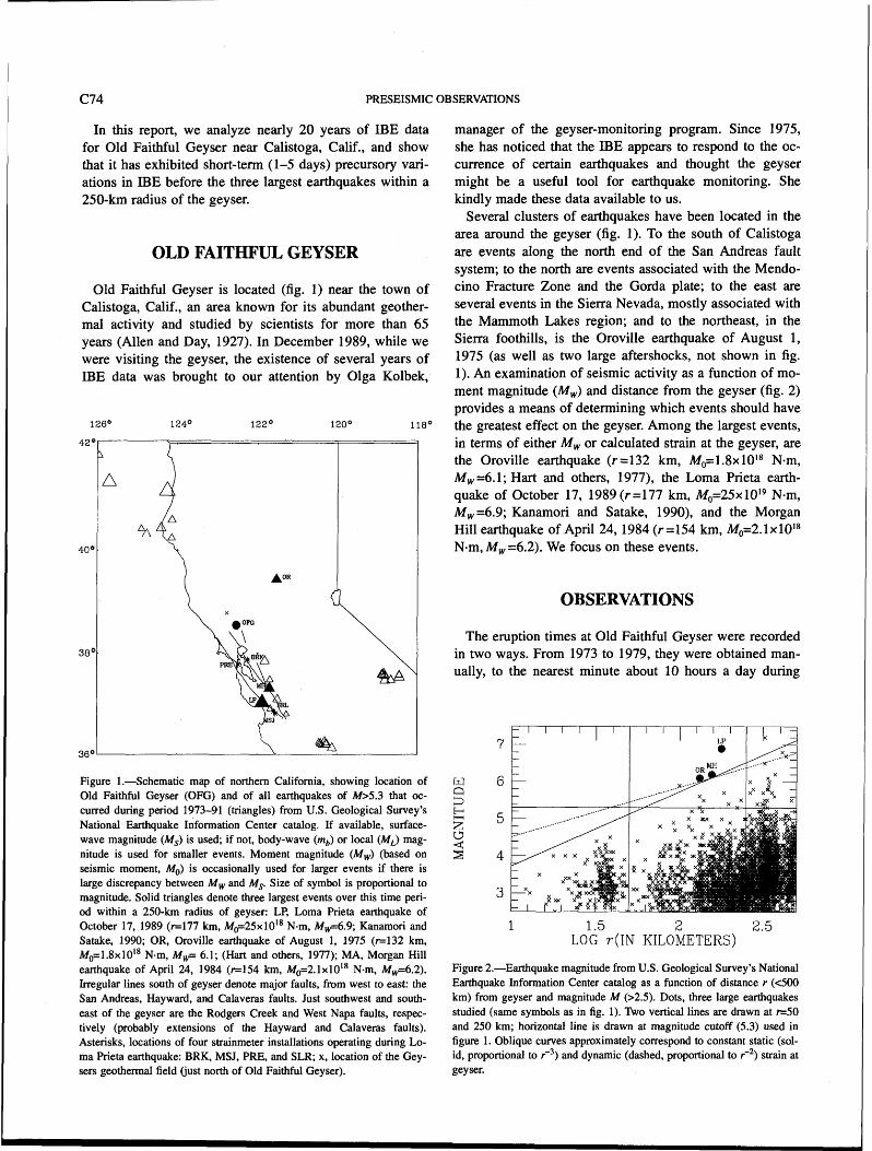
c74 PRESEISMIC OBSERVATIONS
In this report, we analyze nearly 20 years of IBE data for Old Faithful Geyser near Calistoga, Calif., and show that it has exhibited short-term (1-5 days) precursory vari- ations in IBE before the three largest earthquakes within a 250-krn radius of the geyser.
OLD FAITHFUL GEYSER
Old Faithful Geyser is located (fig. 1) near the town of Calistoga, Calif., an area known for its abundant geother- mal activity and studied by scientists for more than 65 years (Allen and Day, 1927). In December 1989, while we were visiting the geyser, the existence of several years of IBE data was brought to our attention by Olga Kolbek,
manager of the geyser-monitoring program. Since 1975, she has noticed that the IBE appears to respond to the oc- currence of certain earthquakes and thought the geyser might be a useful tool for earthquake monitoring. She kindly made these data available to us.
Several clusters of earthquakes have been located in the area around the geyser (fig. 1). To the south of Calistoga are events along the north end of the San Andreas fault system; to the north are events associated with the Mendo- cino Fracture Zone and the Gorda plate; to the east are several events in the Sierra Nevada, mostly associated with the Mammoth Lakes region; and to the northeast, in the Sierra foothills, is the Oroville earthquake of August 1, 1975 (as well as two large aftershocks, not shown in fig. 1). An examination of seismic activity as a function of mo- ment magnitude (Mw) and distance from the geyser (fig. 2) provides a means of determining which events should have the greatest effect on the geyser. Among the largest events, in terms of either Mw or calculated strain at the geyser, are the Oroville earthquake (r =I32 km, Mo=l .8x loi8 N-m, Mw =6.1; Hart and others, 1977), the Loma Prieta earth- quake of October 17, 1989 (r =I77 km, MO=25xl0l9 Nam, Mw =6.9; Kanamori and Satake, 1990), and the Morgan Hill earthquake of April 24,1984 ( r =I54 km, Mo=2. 1 x loi8 N-m, Mw =6.2). We focus on these events.
OBSERVATIONS
The eruption times at Old Faithful Geyser were recorded in two ways. From 1973 to 1979, they were obtained man- ually, to the nearest minute about 10 hours a day during
Figure 1.-Schematic map of northern California, showing location of Old Faithful Geyser (OFG) and of all earthquakes of M>5.3 that oc- curred during period 1973-91 (triangles) from U.S. Geological Survey's National Earthquake Information Center catalog. If available, surface- wave magnitude (Me) is used; if not, body-wave (mi.) or local (Mi) mag- nitude is used for smaller events. Moment magnitude (My/) (based on seismic moment, Mo) is occasionally used for larger events if there is large discrepancy between Mw and Me. Size of symbol is proportional to magnitude. Solid triangles denote three largest events over this time peri- od within a 250-km radius of geyser: LP, Loma Prieta earthquake of October 17, 1989 ( d 7 7 km, ~ ~ = 2 5 x l 0 ~ * N.m, Mw=6.9; Kanamori and Satake, 1990; OR, Oroville earthquake of August 1, 1975 (-132 km, ~ ~ = 1 . 8 x l 0 ~ ~ N-m, Mw= 6.1; (Hart and others, 1977); MA, Morgan Hill earthquake of April 24, 1984 (r=154 km, ~ ~ = 2 . 1 x l 0 ~ ~ N-m, Mw=6.2). Irregular lines south of geyser denote major faults, from west to east: the San Andreas, Hayward, and Calaveras faults. Just southwest and south- east of the geyser are the Rodgers Creek and West Napa faults, respec- tively (probably extensions of the Hayward and Calaveras faults). Asterisks, locations of four strainmeter installations operating during Lo- ma Prieta earthquake: BRK, MSJ, PRE, and SLR; x, location of the Gey- sers geothermal field (just north of Old Faithful Geyser).
1 1.5 2 2.5 LOG r ( I N KILOMETERS)
Figure 2.-Earthquake magnitude from U.S. Geological Survey's National Earthquake Information Center catalog as a function of distance r (400 km) from geyser and magnitude M (>2.5). Dots, three large earthquakes studied (same symbols as in fig. 1). Two vertical lines are drawn at r=50 and 250 km; horizontal line is drawn at magnitude cutoff (5.3) used in figure 1. Oblique curves approximately correspond to constant static (sol- id, proportional to r 3 ) and dynamic (dashed, proportional to r 2 ) strain at geyser.

DETECTION OF HYDROTHERMAL PRECURSORS TO LARGE NORTHERN CALIFORNIA EARTHQUAKES c75
working hours. Since 1980, they have been recorded auto- matically and continuously by an infrared sensor to the near- est minute for 1980,198 1,1982, and 1990, and to the nearest second for the other years. After checking carefully for tim- ing errors, these data were converted into an IBE time series (fig. 3).' Several well-defined peaks are evident in the IBE data, and the Oroville and Loma Prieta earthquakes coincide with two of them. In addition, during some periods of time the B E displays a multimodal (more than one dominant eruption interval) rather than unimodal (one predominant eruption interval) pattern. The cause of this multimodality is not entirely known, but it is a common feature of other geysers, such as Old Faithful Geyser in Yellowstone Nation- al Park, Wyo. (Rinehart, 1980; Kieffer, 1984; Kieffer, 1989). The time of the Morgan Hill earthquake appears to mark a change from unimodal to multimodal behavior.
RESULTS
For these three large earthquakes, we plotted the IBE records for 1 year of data and for 50 days of data centered
"The data plotted in figure 3 have been passed through a median filter to enhance coherent features. A median filter is similar to the more famil- iar running mean filter, except that the median, rather than the mean, is used. The median is preferred for time series with many isolated outliers, as is the case for the geyser data. This filter preserves the sharpness of steplike changes in a time series. The sample length in figure 3 is 20 samples, corresponding to 15 to 30 hours (see Press and others, p. 818).
around the origin times (fig. 4). The times of the Loma Prieta and Oroville earthquakes correspond to the largest interval-lengthening events within their respective years. For the Loma Prieta earthquake (fig. 4A), the IBE in- creased from 90 to 150 minutes and then returned to its preearthquake value after about 70 days. Similarly, for the Oroville earthquake, the IBE increased from 50 to 120 minutes and returned to its preearthquake value after about 40 days. For the Morgan Hill earthquake, the IBE (fig. 4C) changed from a unimodal (approx 40 minutes) to a trimodal (approx 25, 40, 50 minutes) pattern close to the event time; this pattern then persisted for at least the next 6 months.
More detailed plots (figs. 4D-4F) demonstrate the re- markable correspondence between event time and IBE be- havior and show that the IBE variations began before the earthquakes. Before the Loma Prieta earthquake, the IBE fluctuated around 90 minutes; within 4 days, it rapidly doubled. Closer examination reveals that an IBE lengthen- ing began at least 60 hours before the earthquake and reached a preearthquake value of about 100 minutes, well above the baseline defined by the previous month of data. The event time is seen as a local minimum between the preseismic and coseismic changes. Similarly, an IBE dou- bling began a day before the Oroville earthquake; there is a cluster of points (IBE, approx 80-90 minutes) signifi- cantly above the baseline for the previous month. Finally, the change from a unimodal to a highly scattered trimodal pattern actually occurred about a day before the Morgan Hill earthquake.
YEAR
Figure 3.-Interval before eruption (IBE) at Old Faithful Geyser, Calif. (dots), as a function of time; data have been passed through a median filter to enhance coherent features. Diamonds, magnitudes of events of Ma5.3 within 250 km of geyser; vertical lines are drawn at times of Oroville (OR), Morgan Hill (MH), and Loma Prieta (LP) earthquakes. Data are unavailable for 1987 (lost) and part of 1988 (owing to vandalism at geyser).

C76 PRESEISMIC OBSERVATIONS
We studied in detail the time period corresponding to every other earthquake of M ~ 5 . 2 between 200 and 500 krn away, of M>5.0 within a radius of 200 km, and of M>3.5 less than 50 km away from the geyser. None of these earthquakes coincides (within 1-2 days) with a change in IBE nearly as clearly as the three events plotted in figure 4. The closest earthquakes are the cluster of four relatively large local events (M-4) that occurred in August and Sep- tember 1989 (fig. 4A) about 40 km northwest of the geyser (fig. 1). Finally, none of these other events can provide an adequate explanation for either the preseismic or coseis- mic variations in IBE associated with the three major earthquakes shown in figure 4.
Figure 4.-Interval before eruption (IBE) at Old Faithful Geyser, Calif. (dots), as a function of time. A, Unfiltered IBE data for 1-year period centered on time of Loma Prieta earthquake (vertical line). Diamonds. earthquakes within a 50-km radius of geyser; crossed diamonds, earth- quakes of M-5.3 within 250 km of geyser. Event time coincides with largest episode of IBE lengthening in this period; IBE returned to pre- earthquake levels after about 70 days. Smaller IBE lengthening at 1989.7 may be associated with cluster of four events near the Geysers geothermal field (cross, fig. 1). B, Same as in figure 4A except for Oroville earthquake. Diamonds, main shock and two aftershocks. Event time coincides with largest episode of IBE lengthening in this period; IBE returned to pre- earthquake levels after about 40 days. C, Same as in figure 4A except for
Other physical phenomena might perturb the IBE, such as precipitation, changes in barometric pressure, and local hydrologic variations. These phenomena must be evaluated to ensure that they are not mistaken for changes of tectonic origin. Precipitation appears to have the largest effect. As shown in figure 4C, for example, the drop in IBE of 15 minutes coincides with the largest 1-day value of precipita- tion in the year shown (more than 9 cm). Closer exarnina- tion of the data for the period-6 months before the Morgan Hill earthquake, reveals that daily rainfall of more than 2.5 cm commonly coincided with a nearly instantaneous (with- in 1 day) decrease in IBE (approx 2 minutes in IBE per centimeter of precipitation). The effect of precipitation can
Morgan Hill earthquake. Event time coincides with change from unimodal to multimodal pattern of eruptions. Abrupt decrease in IBE near 1983.9 (arrow) coincides with largest daily precipitation of 9 cm in this period, suggesting that decrease was rain induced. D, Unfiltered IBE data for 50- day period centered on Loma Prieta earthquake. IBE lengthening began about 60 hours (0.0068 year) before earthquake (dashed vertical line). Rapid decreases in IBE after earthquake (arrows) coincide with largest 4- day interval of precipitation in this period, suggesting that decreases were related. E, Same as in figure 4 0 except for Oroville earthquake. IBE lengthening begins about a day before earthquake (dashed vertical line). F, Same as in figure 4D except for Morgan Hill earthquake. Change from unimodal to multimodal behavior occurs about 1 day before earthquake.
DETECTION OF HYDROTHERMAL PRECURSORS TO LARGE NORTHERN CALIFORNIA EARTHQUAKES c77
also be seen for the Loma Prieta earthquake: The largest 4- day period of precipitation of the year, commencing 5 days after the earthquake is closely associated with an abmpt drop in IBE after an initial coseismic rise (fig. 4D).
The most important question is whether precipitation could account for the signals we have attributed to tectonic causes. For the Loma Prieta and Oroville earthquakes, this question would be quite difficult because (1) there was no significant rainfall in the month before the Loma Prieta earthquake and in the 3 months before the Oroville earth- quake, and (2) precipitation appears to induce interval shortening, not interval lengthening. For the Morgan Hill earthquake, the answer is slightly less straightforward be- cause the IBE signal is a mode change, not a lengthening. In addition, although there was no significant rainfall in the month before the earthquake (max 2.5 cm), there was some precipitation (approx 1 cm) 4 and 8 days before the earth- quake. Nevertheless, considering the empirical evidence for an instantaneous IBE response to precipitation and the expected small change in IBE (1-2 minutes) from this
amount of rainfall, precipitation probably did not cause the preseismic and coseismic changes in eruptive mode.
Barometric pressure is another source of stress that plau- sibly can affect the B E . This notion was first considered by Rinehart (1972) for Old Faithful Geyser in Yellowstone National Park, Wyo., using IBE data from 1960 to 1969; he argued for a response on time scales of a year. Most important for our purposes is the effect of barometric pres- sure on the scale of days to weeks; however, we see no clear evidence for such an effect. There are no unusually large excursions in pressure that could plausibly account for the coseismic or preseismic signals that we have attrib- uted to tectonic causes. This conclusion is illustrated for the Loma Prieta earthquake in figure 5. There is, however, an observable indirect relation: An abrupt decrease in barometric pressure commonly precedes precipitation, and, as we have seen, this decrease can cause a corresponding decrease in IBE. This effect is particularly clear for the Loma Prieta and Morgan Hill earthquakes on the days of high precipitation mentioned above.
Figure 5.-3-hourly barometric pressure in San Francisco (upper trace) and extensometer record from station PRE (see fig. 1 for location) along direction N. 73' E. (lower trace) as a function of time for 100-day period before Loma Prieta earthquake. Dots show unfiltered interval-before-eruption (IBE) data from Old Faithful Geyser, Calif., for reference. Positive change in extensometer record corresponds to extension. Predominant periodic signal is due to tidal effects; largest excursion in record is rapid decrease in strain (dotted vertical line) beginning 7 days before earthquake (solid vertical line).
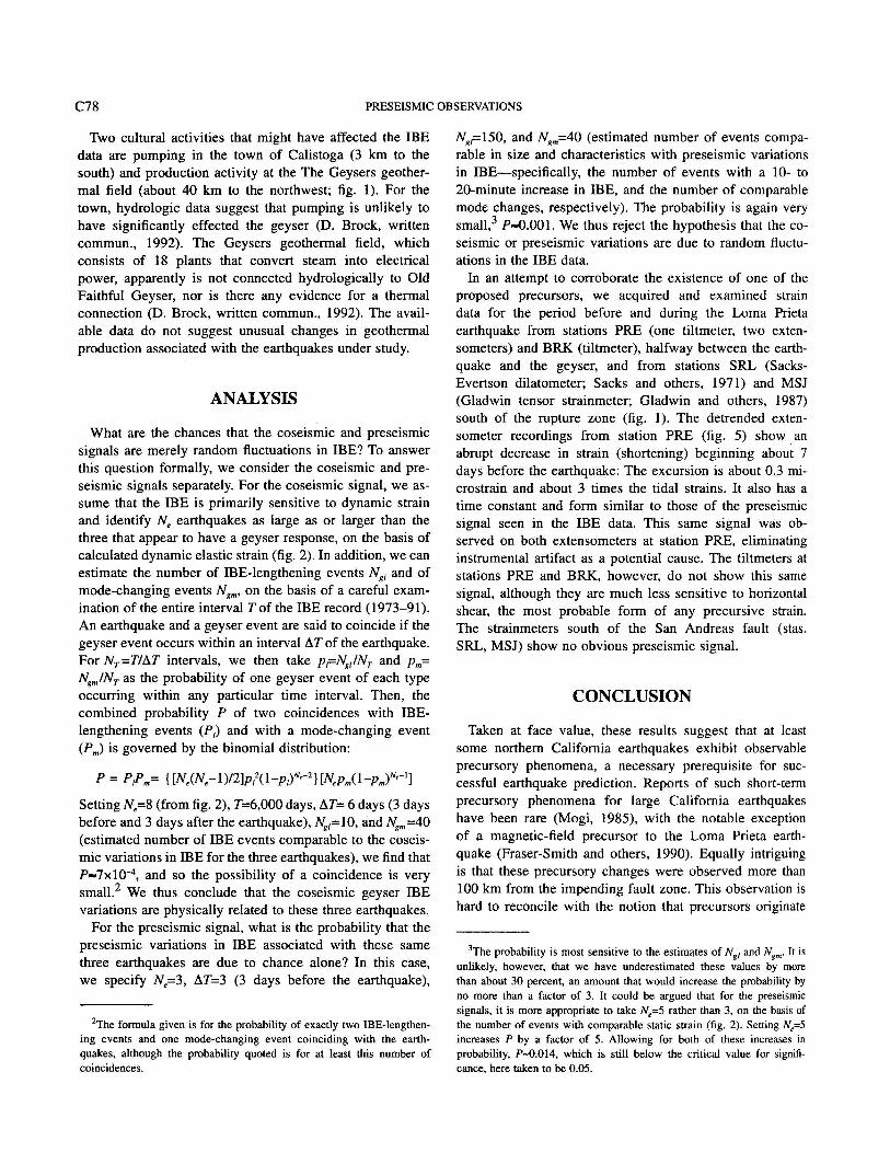
C78 PRESEISMIC OBSERVATIONS
Two cultural activities that might have affected the IBE data are pumping in the town of Calistoga (3 km to the south) and production activity at the The Geysers geother- mal field (about 40 km to the northwest; fig. 1). For the town, hydrologic data suggest that pumping is unlikely to have significantly effected the geyser (D. Brock, written commun., 1992). The Geysers geothermal field, which consists of 18 plants that convert steam into electrical power, apparently is not connected hydrologically to Old Faithful Geyser, nor is there any evidence for a thermal connection (D. Brock, written commun., 1992). The avail- able data do not suggest unusual changes in geothermal production associated with the earthquakes under study.
ANALYSIS
What are the chances that the coseismic and preseisrnic signals are merely random fluctuations in IBE? To answer this question formally, we consider the coseismic and pre- seismic signals separately. For the coseismic signal, we as- sume that the IBE is primarily sensitive to dynamic strain and identify N, earthquakes as large as or larger than the three that appear to have a geyser response, on the basis of calculated dynamic elastic strain (fig. 2). In addition, we can estimate the number of IBE-lengthening events NRi and of mode-changing events Ngm, on the basis of a careful exam- ination of the entire interval T of the IBE record (1973-91). An earthquake and a geyser event are said to coincide if the geyser event occurs within an interval AT of the earthquake. For NT=T/AT intervals, we then take ppNgi/% and pm= NgmWy as the probability of one geyser event of each type occurring within any particular time interval. Then, the combined probability P of two coincidences with IBE- lengthening events (Pi) and with a mode-changing event (Pm) is governed by the binomial distribution:
Setting N,=S (from fig. 2), T=6,000 days, AT= 6 days (3 days before and 3 days after the earthquake), Ngi=lO, and N -40 (estimated number of IBE events comparable to the coseis- mic variations in IBE for the three earthquakes), we find that P-7x10⁴, and so the possibility of a coincidence is very srnalla2 We thus conclude that the coseismic geyser IBE variations are physically related to these three earthquakes.
For the preseismic signal, what is the probability that the preseismic variations in IBE associated with these same three earthquakes are due to chance alone? In this case, we specify Ne=3, AT=3 (3 days before the earthquake),
h he formula given is for the probability of exactly two IBE-lengthen- ing events and one mode-changing event coinciding with the earth- quakes, although the probability quoted is for at least this number of coincidences.
NR,=150, and N - 4 0 (estimated number of events compa- rable in size and characteristics with preseismic variations in IBE-specifically, the number of events with a 10- to 20-minute increase in IBE, and the number of comparable mode changes, respectively). The probability is again very small,3 P-O.OO1. We thus reject the hypothesis that the co- seismic or preseismic variations are due to random fluctu- ations in the IBE data.
In an attempt to corroborate the existence of one of the proposed precursors, we acquired and examined strain data for the period before and during the Loma Prieta earthquake from stations PRE (one tiltmeter, two exten- someters) and BRK (tiltmeter), halfway between the earth- quake and the geyser, and from stations SRL (Sacks- Evertson dilatometer; Sacks and others, 1971) and MSJ (Gladwin tensor strainmeter; Gladwin and others, 1987) south of the rupture zone (fig. 1). The detrended exten- someter recordings from station PRE (fig. 5) show an abrupt decrease in strain (shortening) beginning about 7 days before the earthquake: The excursion is about 0.3 rni- crostrain and about 3 times the tidal strains. It also has a time constant and form similar to those of the preseismic signal seen in the IBE data. This same signal was ob- served on both extensometers at station PRE, eliminating instrumental artifact as a potential cause. The tiltmeters at stations PRE and BRK, however, do not show this same signal, although they are much less sensitive to horizontal shear, the most probable form of any precursive strain. The strainmeters south of the San Andreas fault (stas. SRL, MSJ) show no obvious preseismic signal.
CONCLUSION
Taken at face value, these results suggest that at least some northern California earthquakes exhibit observable precursory phenomena, a necessary prerequisite for suc- cessful earthquake prediction. Reports of such short-term precursory phenomena for large California earthquakes have been rare (Mogi, 1985), with the notable exception of a magnetic-field precursor to the Loma Prieta earth- quake (Fraser-Smith and others, 1990). Equally intriguing is that these precursory changes were observed more than 100 km from the impending fault zone. This observation is hard to reconcile with the notion that precursors originate
on he probability is most sensitive to the estimates of Ngi and Ngm. It is unlikely, however, that we have underestimated these values by more than about 30 percent, an amount that would increase the probability by no more than a factor of 3. It could be argued that for the preseismic signals, it is more appropriate to take Ne=5 rather than 3, on the basis of the number of events with comparable static strain (fig. 2). Setting N,=5 increases P by a factor of 5. Allowing for both of these increases in probability, P-0.014, which is still below the critical value for signifi- cance. here taken to be 0.05.

DETECTION OF HYDROTHERMAL PRECURSORS TO LARGE NORTHERN CALIFORNIA EARTHQUAKES c79
as preseismic slip on the fault. Although the coseismic dy- namic strains for the three earthquakes studied here are calculated to be quite large, about and probably ac- count for the coseismic geyser response, the preseismic static strains would be expected to be much smaller (Roeloffs, 1988), at most to Because we have been unable to detect tidal strains (tidal lines 01, M2) in the IBE data, corresponding to a strain of the strains caused by precursory slip on the fault would be far too small to explain the data. Strains of at least 10"' are proba- bly required and would most likely be due to variations in regional strain that serve to load the impending fault zone. Directional loading of the Loma Prieta rupture zone from the north, for example, could explain the preseismic strain (approx 3 ~ 1 0 ' ~ at station PRE, fig. 5), the presence of a preseismic signal at the geyser, and the absence of such a signal at stations south of the San Andreas fault. The ex- istence of precursory changes in regional strain is suggest- ed by other hydrologic data as well. Indeed, a recent worldwide compilation of precursory hydrologic phenome- na shows that most observations beyond a distance of 150 km from the associated earthquake cannot be explained by preseismic slip (Roeloffs, 1988) and so another mecha- nism, such as regional strain, is probably needed. In addi- tion, a recent statistical approach to earthquake prediction (Keilis-Borok and others, 1988) implies that large regions (several hundred square kilometers) may be involved in the preparatory phase of large seismic events.
How the IBE responds to tectonic strain is not entirely known, although some plausible explanations can be of- fered. The immediate reservoir of Old Faithful Geyser ex- tends to a depth of 70 m and is 30 cm in diameter (Rinehart, 1980); it is recharged by a deep, high-tempera- ture reservoir within fractured volcanic rocks. Temporal variations in IBE are probably controlled by changes in the volumetric-flow velocity Q associated with recharge (Kief- fer, 1989). Here, the closest analogy to the geyser would be the well-drawdown problem for a confined aquifer. As- suming Darcy flow, Q is then proportional to kAH, where k is the permeability and AH is the difference in hydraulic head between the point of recharge (Ho) and the well (HJ. A drop in Ho (increase in IBE) could result from microf- racturing of the confining material and partial draining of the aquifer. Such a mechanism has been proposed to ac- count for the observed striking reduction in well levels (by as much as 20 m) and increased streamflow at a distance of 20 to 40 km from the Loma Prieta earthquake, presumably owing to coseismic deformation (Rojstaczer, 1991). Alter- natively, strain-induced changes in reservoir volume could significantly change Ho if the recharge zone is small in comparison with the reservoir (for example, a narrow fault zone; see Carrigan and others, 1991). Finally, k could change through strain-induced variations in the size of pre- existing microfractures within the reservoir. In hydrologic
systems where fractures are nearly closed, large changes in permeability can occur with strains of about to (Amos Nur, written commun., 1992). Although we cannot at present choose between these mechanisms, they simply illustrate the plausibility of a close relation between the IBE of an Old Faithful-type geyser and tectonic strain.
ACKNOWLEDGMENTS
We thank the workers at Old Faithful Geyser, whose dil- igent monitoring has made this study possible; and D. Power, who along with J. Dunlap and A. Sawyer entered more than 150,000 eruption times into the computer. E. Roeloffs, P. Rydelek, G. Helffrich, and I. Cifuentes re- viewed the manuscript. We also thank A. Linde for numer- ous stimulating conversations, as well as S. Sacks, S. Kieffer, D. White, S. Rojstaczer, S. Hickman, J. Rinehart, C. Carrigan, and D. Brock for helpful discussions. Finally, we thank M. Acierno for computer support and J. Dunlap for assistance with manuscript preparation. This research was sponsored by the Department of Terrestrial Magne- tism, Carnegie Institution of Washington.
REFERENCES CITED
Allen, E.T., and Day, A.L., 1927, Steam wells and other thermal activity at "The Geysers" California: Carnegie Institution of Washington Publication 378, 106 p.
Camgan, C.R., King, G.C.P., Ban-, G.E., and Bixler, N.E., 1991, Poten- tial for water-table excursions induced by seismic events at Yucca Mountain, Nevada: Geology, v. 19, no. 12, p. 1157-1160.
Cifuentes, I.L., and Silver, P.G., 1989, Low-frequency source characteris- tics of the great 1960 Chilean earthquake: Journal of Geophysical Research, v. 94, no. Bl, p. 643-663.
Fraser-Smith, A.C., Bernardi, Arman, McGill, P.R., Ladd, M.E., Helliwell, R.A., and Villard, O.G., Jr., 1990, Low-frequency magnetic field measurements near the epicenter of the Me 7.1 Loma Prieta earth- quake: Geophysical Research Letters, v. 17, no. 9, p. 1465-1468.
Gladwin, M.T., Gwyther, R.L., Hart, R.H.G., Francis, M.F., and Johnston, M.J.S., 1987, Borehole tensor strain measurements in California: Journal of Geophysical Research, v. 92, no. B8, p. 7981-7988.
Gladwin, M.T., Gwyther, R.L., Higbie, J.W., and Hart, R.H.G., 1991, A medium term precursor to the Loma Prieta earthquake?: Geophysi- cal Research Letters, v. 18, no. 8, p. 1377-1380.
Hart, R.S., Butler, Rhett, Kanamori, Hiroo, 1977, Surface-wave con- straints on the August 1, 1975, Oroville earthquake: Seismological Society of America Bulletin, v. 67, no. 1, p. 1-7.
Hutchinson, R.A., 1985, Hydrothermal changes in the upper Geyser Ba- sin, Yellowstone National Park after the 1983 Borah Peak, Idaho, earthquake, in Stein, R.S., and Bucknam, R.C., eds., Proceedings of Workshop XXVIII on the Borah Peak, Idaho earthquake; volume A: U.S. Geological Survey Open-File Report 85-290-A, p. 612-624.
Kanamori, Hiroo, and Satake, Kenji, 1990, Broadband study of the 1989 Loma Prieta earthquake: Geophysical Research Letters, v. 17, no. 8, p. 1179-1182.
Kanamori, Hiroo, and Cipar, J.J., 1974, Focal process of the great Chil- ean earthquake May 22, 1960: Physics of the Earth and Planetary Interiors, v. 9, p. 128-136.

C80 PRESEISMIC OBSERVATIONS
Keilis-Borok, V.I., Knopoff, Leon, Rotwain, LM., and Allen, C.R., 1988, Intermediate-term prediction of occurrence times of strong earth- quakes: Nature, v. 335, no. 6192, p. 690-694.
Kieffer, S.W., 1984, Seismicity at Old Faithful Geyser; an isolated source of geothermal noise and possible analogue of volcanic seismicity: Journal of Volcanology and Geothermal Research, v. 22, no. 1-2, p. 59-95.
1989, Geologic nozzles: Reviews of Geophysics, v. 27, no. 1, p. 3-38.
Kissin, I.G., and Grinevsky, A.O., 1990, Main features of hydrogeodynamic earthquake precursors: Tectonophysics, v. 178, no. 2-4, p. 277-286.
Linde, A.T., Suyehiro, Kiyoshi, Miura, Satoshi, Sacks, IS., and Takagi, Akio, 1988, Episodic aseismic earthquake precursors: Nature, v. 334, no. 6182, p. 513-515.
Mogi, Kiyoo, 1985, Earthquake prediction: Tokyo, Academic Press, 355 p. Press, W.H., Flannery, B.P., Teukolsky, S.A., and Vetterling, W.T., 1986,
Numerical modeling: Cambridge, U.K., Cambridge University Press. Rinehart, J.S., 1972, Fluctuations in geyser activity caused by variations
in earth tidal forces, barometric pressure, and tectonic stresses: Jour- nal of Geophysical Research, v. 77, no. 2, p. 342-350.
1980, Geysers and geothermal energy: New York, Springer-Ver- lag, 223 p.
Roeloffs, E.A., 1988, Hydrologic precursors to earthquakes; a review: Pure and Applied Geophysics, v. 126, no. 2-4, p. 177-209.
Rojstaczer, S.A., 1991, Elastic deformation as a second order influence on groundwater flow in areas of crustal unrest [abs.]: Eos (Ameri- can Geophysical Union Transactions), v. 72, no. 17, p. 121.
Sacks, I.S., Suyehiro, Shigeji, Evertson, D.W., and Yamagishi, Yoshiaki, 1971, Sacks-Evertson strainmeter, its installation in Japan and some preliminary results concerning strain steps: Papers in Meteorology and Geophysics, v. 22, p. 195-207.
Silver, P.G., and Valette-Silver, N.J., 1987, A spreading episode at the southern end of the San Andreas fault system: Nature, v. 326, no. 6113, p. 589-593.
Wood, S.H., 1985, Regional increase in groundwater discharge after the 1983 Idaho earthquake; coseismic strain release, tectonic and natu- ral hydraulic fracturing, in Stein, R.S., and Bucknam, R.C., eds., Proceedings of Workshop XXVII on the Borah Peak, Idaho earth- quake; volume A: U.S. Geological Survey Open-File Report 85- 290-A, p. 573-592.
THE LOMA PRIETA, CALIFORNIA, EARTHQUAKE OF OCTOBER 17,198k m R m Q U A K E O C C U m N C E
PRESEISMIC OBSERVATIONS
BOREHOLE STRAIN MEASUREMENTS OF SOLm-EARTH-TmAL AMPLITUDES
By Alan T. Linde, Carnegie Institution of Washington; Michael T. Gladwin, University of Queensland, Australia; and
Malcolm J.S. Johnston, U S . Geological Survey
CONTENTS
ABSTRACT
The Loma Prieta earthquake pmvided an opportunity for a sensitive test of suggestions that earthquakes may be preceded by variations in earth-tidal strain amplitudes. Such variations have been pmposed as providing an ad- vantageous technique for detecting precursory changes in elastic parameters within a seismogenic zone. We have an- alyzed the data from two borehole strainmeters continu- ously operating within 40 km of the epicenter and within about 10 km of the south end of the rupture zone. We are unable to identify any precursory changes in tidal compo- nents M2 and 01 and estimate that any large-scale chang- es in Young's modulus must have been less than about 2 percent. If these results apply generally, we conclude that variations in elastic material properties before earthquakes do not occur throughout substantial volumes of the subse- quent hypocentral region.
INTRODUCTION
Nishimura (1950) first suggested that changes in earth- tidal response might be a useful method for monitoring crustal elastic properties and, possibly, predicting earth- quakes. Several other studies have been made on the tem- poral variations of tidal amplitudes in seismically active regions (for example, Mikumo and others, 1978; Kato, 1979; Ma0 and others, 1989), but none of these studies has provided strong evidence to support or refute the use- fulness of the technique for earthquake prediction. Finite-
element analysis has been used (Beaumont and Berger, 1974; Tanaka, 1976) to calculate tidal-response anomalies as a function of changes in the elastic properties of vari- ous-shaped source regions.
The Loma Prieta earthquake was the largest California earthquake in recent years and the largest to occur relatively close to any of the continuous strain-monitoring stations in California. Elsewhere (Johnston and others, 1990), we have reported on the absence of observed short-tern strain precur- sors to this earthquake. Johnston and Linde (1990), in a pre- liminary analysis of the data from one of these stations, re- ported on a precursory tidal-amplitude anomaly for this earth- quake, but their analysis included then-undetected artifacts in the data. We have now analyzed the data from two stations to determine whether any significant changes in tidal amplitudes occurred during the several years before the earthquake.
Initial plans for borehole strain instrumentation in the San Juan Bautista, Calif., area, just south of the Loma Prieta rupture zone (fig. l), called for the installation of a modest network of five to seven stations. Owing to various con- straints, however, only three instruments were installed, two of which were in operation during the study period: a tensor (three component) strainmeter (Gladwin and others, 1986) and a Sacks-Evertson strainmeter (dilatometer) (Sacks and others, 1971). The locations of these two stations in relation to the Loma Prieta rupture zone are mapped in figure 1; the tensor strainmeter (sta. SJT) is 38 km from the epicenter, and the dilatometer (sta. SRL) 33 km. The instrumental data are collected at the U.S. Geologi-
cal Survey offices in Men10 Park, Calif., via satellite digital telemetry (Silverman and others, 1989); station SJT is sam- pled every 18 minutes, and station SRL every 10 minutes. Both instruments have more than adequate sensitivity and frequency response to ensure that Earth tides can be detect- ed and recorded with good precision.
ANALYSIS We concentrate our analysis on the strain data from the
approximately 2-year period before the earthquake. Our

C82 PRESEISMIC OBSERVATIONS
conclusions apply to earlier data also, but for various tech- nical reasons (postinstallation effects, various instrument modifications, and less reliable telemetry) the earlier data vary more widely. For the period shown in figures 2 and 3, station SJT has been operating without modification, and the data stream has been consistently reliable and un- disturbed by site visits. Several problems, however, have complicated the record from station SRL. We have re- moved from the record any artifacts introduced by site vis- its, although we suspect that, after mid-March 1989, the data from station SRL may have been subjected to a slow- ly decreasing effective gain, apparent during 1990.
The tidal analyses have been carried out by using two inde- pendent procedures: a linear least-squares inversion (Glad- win and others, 1985). and the BAYTAP(G) routine based on Bayesian statistics (Ishiguro and others, 1984). Excellent agreement was obtained for the calculated tidal amplitudes. We have performed various tests with both real and synthetic data to ensure that the results are reliable and robust. Tempo- ral variations in tidal components M2 and 0 1 at the two stations are plotted in figure 2. We have used 60-day win- dows for our analysis, with sequential windows sliding for- ward by 30 days. The time tag associated with each analysis is taken as the midpoint of the window. From station SRL we obtain estimates of the dilatational strain. The instrument at station SJT records three components of strain, defined by
where the x-axis is east and the y-axis north. Note that all of the traces are characterized by long-term constancy of both tidal components M2 and 01. Formal error bars (lo) are given for all points, and in some places, particularly for the larger-amplitude signals, these error bars are obscured by the data points, In general, as we would expect, the errors are larger for smaller-amplitude signals, which are all shown at their absolute levels. Confidence in the reliability of our measurements is also enhanced by the fact that the M2-to-01 tidal-amplitude ratios for all strain components agree well with the theoretically calculated ratios. For all the tidal-amplitude signals, no variations are evident that can be considered significant in the 2-year period before the earthquake. The standard deviations of these values are about 1 percent for the M2 components of ea and V (dilata- tion) amplitudes, about 2 percent for the corresponding 0 1 components, and somewhat larger for the lower-amplitude tidal components. We estimate the threshold for detecting departures from constancy at about the 2-percent level.
During 1990, the instmment at station SRL has been characterized by a clear, steady decrease in gain due to the accumulated effects of a 1987 downhole leak in the cable or at the cablehead. A modification in the electronics al- lowed stable operation of the instrument, as evidenced by the constancy of the tidal admittance during 1988, but an inadvertent modification in March 1989 (asterisks, fig. 2) partly restored the pre-1987 configuration. (The instanta- neous gain change caused by this modification has been removed from the data.) This instrument measures dilata- tional strain, and because variations in atmospheric pres- sure cause corresponding changes in dilatational strain in the near-surface rock, we can check for changes in instru- mental gain by calculating the pressure admittance versus time. The pressure admittance and tidal components M2 (fig. 3A) and 0 1 (fig. 3B) versus time at station SRL after the March 1989 modification are plotted in figure 3; a faulty pressure transducer was also replaced at that time. Although we do not expect the pressure admittance and tidal amplitudes to track precisely (the effective bulk mod- ulus of near-surface material varies with, for example, ground-water content), starting at about 1990 both the pressure admittance and tidal amplitudes clearly show sim- ilar and consistent decreases. We have used the pressure admittance as a gain correction to the tidal amplitudes (cir- cles and dashed curves, fig. 2). This correction results in nearly constant tidal amplitudes until about mid-1990, when a real decrease in the pressure admittance may have occurred, and so the correction produces larger tidal ampli- tudes. The need for correcting these post-1990 tidal ampli- tudes somewhat decreases the weight we can give to these measurements from station SRL, but it appears that the postseismic tidal components M2 and 0 1 -it station SRL
Figure 1.-bma Prieta region, Calif., showing locations of mo~toring stations (squares) and major faults (lines). Heavy line, b m a Prieta mp- did not change significantly, consistent with their constan-
mne; s m , epicenem of b m a Keta e a t h q d e (large) and I.,&= CY at station SJT. (Note that these reservations do not ~ P P ~ Y Elsman foreshocks of 1988 and 1989 (small). to the preseismic and coseismic data from station SRL.)

BOREHOLE STRAIN MEASUREMENTS OF SOLID-EARTH-TIDAL AMPLITUDES C83
We do not detect any coseismic change in Earth tidal- strain amplitudes (at the 2-percent level), and the tidal am- plitudes after the earthquake are at the same levels as be- fore. Thus, any changes in elastic parameters introduced as a result of rock fracturing during the earthquake were also quite small or localized to a small volume. If we had re- ported a precursory effect without noticing any coseismic change, we might have questioned the validity of that re- sult, although for this type of phenomenon the absence of such change does not necessarily exclude the possibility of recording any precursory effect.
DISCUSSION
The finite-element models of Beaumont and Berger (1974) and Tanaka (1976) were published when dilatancy
was thought to be a wide-scale precursory phenomenon. The modeling estimates by Beaumont and Berger of varia- tions as large as 60 percent in tidal strain were based on large dilatant zones in which the seismic compressional- wave velocity was reduced by 15 percent. Although large effects are no longer considered likely, we can use our re- sults to place upper constraints on any precursory strain- induced variations in the elastic properties of the seismo- genic zone for the earthquake. The modeling by Beaumont and Berger indicates that our stations are favorably located for detection of any significant variations in elastic proper- ties within the site region. If such changes occurred before the earthquake, these stations would surely have been with- in about 30 km of such a zone, possibly as close as 10 or 15 km. Beaumont and Berger's work shows that this situa- tion would provide near-maximum sensitivity for detection
1988 1988.5 1989 1989.5 1990 1990.5 1991
YEAR
Figure 2.-Earth-tidal strain amplitudes of components M2 and 0 1 as a function of time at stations SRL and SJT (see fig. 1 for locations). Error bars are lo. LP, time of Loma Prieta earthquake; stars, time of an electronic change at station SRL (see text). Since 1990. data from station SRL have been gain corrected, using atmospheric-pressure response (dashed curves with circles). Larger values near end of station SRL traces apparently result from an overcorrection. We find no significant variations in these amplitudes before earthquake. Note also that earthquake has not had any significant coseismic or postseismic effect on tidal amplitudes.

C84 PRESEISMIC OBSERVATIONS
and that, even for a more remote source, the stations would be well placed to record the resulting tidal-amplitude changes. If such changes did occur, then changes in Young's modulus over any large (kilometers) spatial extent must have been less than about 2 percent. The correspond- ing change in V would be less than about 1 percent, a limit lower than that set from traveltime residuals for local earthquakes (Steppe and others, 1977) or for teleseismic events (Robinson and lyer, 1976). The alternative possibil- ity, which we cannot exclude, is that significant changes in Young's modulus occurred within a small preparation zone. Although this issue may remain important in the me- chanics of rupture, it appears to be academic in terms of precursor detection because we do not know the location
Figure 3.-Pressure admittance (circles) and tidal amplitudes (dots) of components M2 (A) and 0 1 (5) versus time at station SRL (fig. 1) after March 1989 electronic modification. Pressure admittance is negative be- cause an increase in atmospheric pressure causes contraction (negative strain) in near-surface rock. Although pressure admittance changes over time, both tidal amplitudes and pressure admittances clearly decrease systematically during 1990, owing to a slowly decreasing effective gain of instrument during that period.
- 1 - l l l l l l l l l l l l l l l t -
of initiation of a future earthquake and, in many cases, cannot physically locate instruments near such a location even if we did know it exactly.
We conclude that no identifiable (greater than 2 percent) precursory changes in solid-earth-tidal amplitudes oc- curred in the area about 35 km to the south of the epicen- ter. This result places a significant constraint on such precursory effects and corrects an earlier report of a posi- tive result for this effect: the preliminary work by Johnston and Linde (1990) was in error, principally be- cause not all the effects of electronic modifications to the instrument at station SRL were recognized and removed from the data at that time. The results obtained here are consistent with the report by Gladwin and others (1991), who noted the constancy of earth-tidal strain amplitudes before the earthquake. To the extent that our observations at the two stations can be generalized, it now appears less likely that variations in earth-tidal strain amplitudes can serve as earthquake precursors.
-2.0
ACKNOWLEDGMENTS
1989.5 1990 1990.5 1991 YEAR
Doug Myren provided valuable help in the operation of station SRL, and we appreciate the work of Kate Brecken- ridge in maintaining the data-acquisition files. Duncan Ag- new first noted that a site visit may have been overlooked in the preliminary work. We thank Y. Tamura for supplying a copy of the BAYTAP(G) analysis program and for dis- cussions on its use. The second author was supported in part by U.S. Geological Survey grant 14-08-0001-Gl376; the first author was supported in part by a grant from the Bilateral Science and Technology Program, Australian De- partment of Industry, Technology and Commerce, and in part by U.S. Geological Survey Grant 14-08-0001-G2064.
REFERENCES CITED
Beaumont, Christopher, and Berger, Jon, 1974, Earthquake prediction; modification of the Earth tide tilts and strains by dilatancy: Royal Astronomical Society Geophysical Journal, v. 39, no. 1, p. 11 1-121.
Gladwin, M.T., Gwyther, R.L., and Hart, R.H.G., 1985, Tidal calibration of borehole vector strain instruments [abs.]: Eos (American Geo- physical Union Transactions), v. 66, no. 46, p. 1057.
Gladwin, M.T., Gwyther, R.L., Hart, R.H.G., Francis, M.F., and Johnston, M.J.S., 1986, Borehole tensor strain measurements in California: Journal of Geophysical Research, v. 92, no. B8, p. 7981-7988.
Gladwin, M.T., Gwyther, R.L., Higbie, J.W., and Hart. R.H.G., 1991, A medium term precursor to the Lorna Prieta earthquake?: Geophysi- cal Research Letters, v. 18, no. 8, p. 1377-1380.
Ishiguro, M., Sato, Takahiro, Tamura, Y., and Ooe, Masatsugu, 1984, Tidal data analysis-an introduction to Baytap: Institute of Statisti- cal Mathematics Proceedings, v. 32, p. 71-85.
Johnston, M.J.S., and Linde, A.T., 1990, Possible change in Earth tidal response before the October 18, 1989, Loma Prieta ML 7.1 earth- quake [abs,]: EQS (American Geophysical Union Transactions), v. 71, no. 43, p. 1461.

BOREHOLE STRAIN MEASUREMENTS OF SOLID-EARTH-TIDAL AMPLITUDES C85
Johnston, M.J.S., Linde, A.T., and Gladwin, M.T., 1990, Near-field high resolution strain measurements prior to the October 18, 1989, Loma Prieta, Mr 7.1 earthquake: Geophysical Research Letters, v. 17, no. 10, p. 1777-1780.
Kato, Masaaki, 1979, Observations of crustal movements by newly-de- signed horizontal pendulum and water-tube tiltmeters with electro- magnetic transducers (2): Kyoto, Japan, Kyoto University, Disaster Prevention Research Institute Bulletin, v. 29, p. 83-97.
Mao, W.J., Ebblin, C., and Zadro, M., 1989, Evidence for variations of mechanical properties in the Friuli seismic area: Tectonophysics, v. 170, no. 3-4, p. 231-242.
Mikumo, Takeshi, Kato, Masaaki, h i , Hikaru, Wada, Yasuo, Tanaka, Torao, Shichi, Ryuichi, and Yamaxnoto, Atsuyuki, 1978, Possibility of temporal variations in Earth tidal strain amplitudes associated with major earthquakes, in Kisslinger, Carl, and Suzuki, Ziro, eds., Earthquake precursors; proceedings of the US-Japan Seminar on Theoretical and Experimental Investigations of Earthquake Precur- SOTS: Tokyo, Center for Academic Publications Japan, p. 123-136.
Nishimura, Eiichi, 1950, On Earth tides: American Geophysical Union Transactions, v. 31, no. 3, p. 357-376.
Robinson, Russell, and Iyer, H.M., 1976, Temporal and spatial variations of travel-time residuals in central California for Novaya Zemlya events: Seismological Society of America Bulletin, v. 66, no. 5, p. 1733-1 747.
Sacks, I.S., Suyehiro, Shigeji, Evertson, D.W., and Yamagishi, Yoshiaki, 1971, Sacks-Evertson strainmeter, its installation in Japan and some preliminary results concerning strain steps: Papers in Meteorology and Geophysics, v. 22, p. 195-207.
Silverman, Stan, Mortensen, C.E., and Johnston, M.J.S., 1989, A satel- lite-based digital data system for low-frequency geophysical data: Seismological Society of America Bulletin, v. 79, no. 1, p. 189-198.
Steppe, J.A., Bakun, W.H., and Bufe, C.G., 1977, Temporal stability of P-velocity anisotropy before earthquakes in central California: Seis- mological Society of America Bulletin, v. 67, no. 4, p. 1075-1090.
Tanaka, Torao, 1976, Effect of dilatancy on ocean load tides: Pure and Applied Geophysics, v. 114, p. 415-423.