DRAFTParticulate Matter CEMS Demonstration

Volume I: DuPont, Inc. Experimental Station On-SiteIncinerator, Wilmington, DE

U.S. Environmental Protection AgencyOffice of Solid Waste and Emergency Response (5305)401 M Street, SWWashington, DC 20460

December 1997

ACKNOWLEDGEMENT

This document was prepared by EPA’s Office of Solid Waste, Hazardous WasteMinimization and Management Division. Energy and Environmental Research Corporation(EER) provided technical support under EPA Contract No. 68-D2-0164. H. Scott Rauenzahnwas EPA’s Work Assignment Manager.

i

TABLE OF CONTENTSSection Page

1.0 INTRODUCTION . . . . . . . . . . . . . . . . . . . . . . . . . . . . . . . . . . . . . . . . . . . . . . . . . . 1-11.1 Demonstration Program Goal and Course of Development . . . . . . . . . . . . . . 1-31.2 Demonstration Program . . . . . . . . . . . . . . . . . . . . . . . . . . . . . . . . . . . . . . . . 1-9

1.2.1 Site Selection Rationale . . . . . . . . . . . . . . . . . . . . . . . . . . . . . . . . . . 1-101.2.2 Achievements and Apparent Limitations of the

Demonstration Program . . . . . . . . . . . . . . . . . . . . . . . . . . . . . . . . . . 1-111.3 Program Overview . . . . . . . . . . . . . . . . . . . . . . . . . . . . . . . . . . . . . . . . . . . . 1-121.4 Description of Facility and Monitors . . . . . . . . . . . . . . . . . . . . . . . . . . . . . . . 1-15

1.4.1 General Facility Description . . . . . . . . . . . . . . . . . . . . . . . . . . . . . . . 1-151.4.2 General Description of CEMS Technologies . . . . . . . . . . . . . . . . . . . 1-17

1.5 Program Scope . . . . . . . . . . . . . . . . . . . . . . . . . . . . . . . . . . . . . . . . . . . . . . . 1-20

2.0 TEST PROGRAM RESULTS . . . . . . . . . . . . . . . . . . . . . . . . . . . . . . . . . . . . . . . . . 2-12.1 Proposed Performance Specifications Calibration Testing . . . . . . . . . . . . . . . 2-22.2 Reference Method Protocol and Treatment of its Outliers . . . . . . . . . . . . . . . 2-4

2.2.1 Reference Method Protocol for the Demonstration Program . . . . . . . 2-42.2.2 Discussion of Outliers . . . . . . . . . . . . . . . . . . . . . . . . . . . . . . . . . . . . 2-7

2.3 Facility Operation Summary . . . . . . . . . . . . . . . . . . . . . . . . . . . . . . . . . . . . . 2-112.3.1 Facility Operation During RCA Testing . . . . . . . . . . . . . . . . . . . . . . . 2-152.3.2 Summary of Facility Operation Over the Test Program . . . . . . . . . . . 2-16

2.4 CEMS Calibration Relation Test Results . . . . . . . . . . . . . . . . . . . . . . . . . . . . 2-172.5 CEMS RCA Test Results . . . . . . . . . . . . . . . . . . . . . . . . . . . . . . . . . . . . . . . 2-292.6 Supporting Data . . . . . . . . . . . . . . . . . . . . . . . . . . . . . . . . . . . . . . . . . . . . . . 2-33

2.6.1 Cumulative Database . . . . . . . . . . . . . . . . . . . . . . . . . . . . . . . . . . . . 2-342.6.2 Scanning Electron Microscope Results . . . . . . . . . . . . . . . . . . . . . . . 2-35

2.6.2.1 Initial Analyses . . . . . . . . . . . . . . . . . . . . . . . . . . . . . . . . . 2-352.6.2.2 Additional Method 5 Filter Analysis Data . . . . . . . . . . . . . 2-36

2.6.3 Comparison of Like-technology Measurement Data . . . . . . . . . . . . . 2-372.6.4 1996 Trial Burn M5/CEMS Data Evaluation . . . . . . . . . . . . . . . . . . . 2-392.6.5 Particle Size Data . . . . . . . . . . . . . . . . . . . . . . . . . . . . . . . . . . . . . . . 2-402.6.6 Rollins and Lafarge PM CEMS Results . . . . . . . . . . . . . . . . . . . . . . . 2-41

2.7 Assessment of PM CEMS Cost and Data Availability . . . . . . . . . . . . . . . . . . 2-452.7.1 Preliminary Cost Assessment . . . . . . . . . . . . . . . . . . . . . . . . . . . . . . . 2-452.7.2 Preliminary Assessment of Data Availability . . . . . . . . . . . . . . . . . . . 2-47

2.8 Summary and Conclusions . . . . . . . . . . . . . . . . . . . . . . . . . . . . . . . . . . . . . . 2-49

3.0 TEST PROGRAM PROTOCOL . . . . . . . . . . . . . . . . . . . . . . . . . . . . . . . . . . . . . . . 3-13.1 Reference Method and CEMS Sampling Locations . . . . . . . . . . . . . . . . . . . . 3-63.2 Reference Method Sampling Procedures . . . . . . . . . . . . . . . . . . . . . . . . . . . . 3-6

3.2.1 Sample Train Description and Sampling Procedures . . . . . . . . . . . . . 3-9

ii

TABLE OF CONTENTS (Cont.)

Section Page

3.2.2 Calibration Procedures . . . . . . . . . . . . . . . . . . . . . . . . . . . . . . . . . . . 3-133.2.3 Data Reduction, Validation, and Reporting . . . . . . . . . . . . . . . . . . . 3-163.2.4 Sample Tracking, Shipping, Storage, and Custody Procedures . . . . . 3-18

3.3 CEMS Sampling and Analysis . . . . . . . . . . . . . . . . . . . . . . . . . . . . . . . . . . . . 3-183.3.1 Verewa F-904-KD Beta Gauge Monitor . . . . . . . . . . . . . . . . . . . . . . 3-193.3.2 Emissions SA 5M Beta Gauge Monitor . . . . . . . . . . . . . . . . . . . . . . . 3-213.3.3 Durag DR-300 Light-scattering Monitor . . . . . . . . . . . . . . . . . . . . . . 3-213.3.4 ESC P5A Light-scattering Monitor . . . . . . . . . . . . . . . . . . . . . . . . . . 3-223.3.5 Sigrist KTNR Light-scattering Monitor . . . . . . . . . . . . . . . . . . . . . . . 3-223.3.6 Jonas, Inc. . . . . . . . . . . . . . . . . . . . . . . . . . . . . . . . . . . . . . . . . . . . . . 3-233.3.7 CEMS Data Acquisition System . . . . . . . . . . . . . . . . . . . . . . . . . . . . 3-23

3.4 Scanning Electron Microscope Analytical Procedure . . . . . . . . . . . . . . . . . . 3-243.5 Process Data Acquisition . . . . . . . . . . . . . . . . . . . . . . . . . . . . . . . . . . . . . . . 3-24

4.0 QUALITY ASSURANCE/QUALITY CONTROL . . . . . . . . . . . . . . . . . . . . . . . . . 4-14.1 Quality Assurance Objectives . . . . . . . . . . . . . . . . . . . . . . . . . . . . . . . . . . . . 4-34.2 Reference Method QC . . . . . . . . . . . . . . . . . . . . . . . . . . . . . . . . . . . . . . . . . 4-6

4.2.1 Quality Control Procedures . . . . . . . . . . . . . . . . . . . . . . . . . . . . . . . . 4-74.2.2 QC for Flue Gas Sampling and Analysis . . . . . . . . . . . . . . . . . . . . . . 4-7

4.3 Field Data Reduction . . . . . . . . . . . . . . . . . . . . . . . . . . . . . . . . . . . . . . . . . . 4-104.3.1 Manual Methods Data Reduction . . . . . . . . . . . . . . . . . . . . . . . . . . . 4-124.3.2 Data Validation . . . . . . . . . . . . . . . . . . . . . . . . . . . . . . . . . . . . . . . . . 4-13

4.4 CEMS Data Acquisition/Reduction . . . . . . . . . . . . . . . . . . . . . . . . . . . . . . . 4-15

iii

APPENDICES

A - Modified Method 5 Evaluation and Procedure - Lab and Field StudyB - Method 5C - Calibration DataD - CEMS Minute Response Data During Monthly TestsE - Calibration RelationsF - Summary of Process Data During Test PeriodsG - Preliminary PM CEMS Test Sites Supporting DataH - Trial BurnI - Filter AnalysisJ - Particle Size ReportK - Revised Draft PS 11L - Draft Appendix FM - Draft Method 5iN - PM CEMS CostsO - Source for ISO 10155P - CEMS Maintenance LogsQ - PM CEMS Vendor SpecificationsR - CEMS Zero and Span Calibration Drift DataS - PM CEMS Continuous Raw DataT - Flue Gas ParametersU - PM CEMS Responses Converted to mg/dscm at 7% O2

V - PM CEMS Converted Data - Three-Hour Rolling Average

iv

LIST OF TABLES

Section Page

Table 2-1 Matrix of Calibration Relation Conditions . . . . . . . . . . . . . . . . . . . . . . . . . . . 2-52Table 2-2 Process Data from Monthly Tests . . . . . . . . . . . . . . . . . . . . . . . . . . . . . . . . . 2-53 Table 2-3 Summary of Method 5 Run Data and RSD . . . . . . . . . . . . . . . . . . . . . . . . . 2-63Table 2-4 CEMS PM Results . . . . . . . . . . . . . . . . . . . . . . . . . . . . . . . . . . . . . . . . . . . 2-72Table 2-5 Results of Linear Calibration Relation . . . . . . . . . . . . . . . . . . . . . . . . . . . . . . 2-76 Table 2-6 Calibration Range Effects on Linear Regression . . . . . . . . . . . . . . . . . . . . . . 2-77Table 2-7 Results of ESC and Sigrist Logarithmic Calibration Relations . . . . . . . . . . . 2-78Table 2-8 Summary of RCA Evaluation Results . . . . . . . . . . . . . . . . . . . . . . . . . . . . . 2-79Table 2-9 Summary of Cumulative Calibration Results . . . . . . . . . . . . . . . . . . . . . . . . 2-80Table 2-10 SEM / EDS Analytical Results of Filters . . . . . . . . . . . . . . . . . . . . . . . . . . . 2-81Table 2-11 Trial Burn Method 5 Results Summary . . . . . . . . . . . . . . . . . . . . . . . . . . . . 2-82Table 2-12 PM CEMS Data During Trial Burn . . . . . . . . . . . . . . . . . . . . . . . . . . . . . . . 2-83Table 2-13 RCA Evaluation Results for Trial Burn Data . . . . . . . . . . . . . . . . . . . . . . . . . 2-84Table 2-14 Summary of Particle Size Results . . . . . . . . . . . . . . . . . . . . . . . . . . . . . . . . . 2-85Table 2-15 Rollins Method 5 Summary . . . . . . . . . . . . . . . . . . . . . . . . . . . . . . . . . . . . . 2-86Table 2-16 Rollins CEMS Summary . . . . . . . . . . . . . . . . . . . . . . . . . . . . . . . . . . . . . . . . 2-88Table 2-17 Rollins and Lafarge Calibration Relation Results . . . . . . . . . . . . . . . . . . . . . . 2-89Table 2-18 Lafarge Method 5 Summary . . . . . . . . . . . . . . . . . . . . . . . . . . . . . . . . . . . . . 2-90Table 2-19 Lafarge CEMS Summary . . . . . . . . . . . . . . . . . . . . . . . . . . . . . . . . . . . . . . . 2-92Table 2-20 PM CEMS Estimated Cost Summary . . . . . . . . . . . . . . . . . . . . . . . . . . . . . . 2-93Table 3-1 Summary of PM/CEMS Characteristics . . . . . . . . . . . . . . . . . . . . . . . . . . . . 3-20Table 4-1 Summary of QA/QC for Stack Gas Examples . . . . . . . . . . . . . . . . . . . . . . . . 4-11

v

LIST OF FIGURES

Section Page

Figure 2-1 Comparison of ESA Linear Calibration Relations . . . . . . . . . . . . . . . . . . . . . 2-94Figure 2-2 Comparison of Verewa Linear Calibration Relations . . . . . . . . . . . . . . . . . . . 2-95Figure 2-3 Comparison of Durag Linear Calibration Relations . . . . . . . . . . . . . . . . . . . . 2-96Figure 2-4 Comparison of ESC Linear Calibration Relations . . . . . . . . . . . . . . . . . . . . . 2-97Figure 2-5 Comparison of Sigrist Linear Calibration Relations . . . . . . . . . . . . . . . . . . . . 2-98Figure 2-6 Comparison of ESC Quadratic Calibration Relations . . . . . . . . . . . . . . . . . . . 2-99Figure 2-7 Comparison of Sigrist Quadratic Calibration Relations . . . . . . . . . . . . . . . . . 2-100Figure 2-8 Statistical Evaluation of ESC Logarithmic Relation

for Initial Calibration . . . . . . . . . . . . . . . . . . . . . . . . . . . . . . . . . . . . . . . . . . 2-101Figure 2-9 Statistical Evaluation of ESC Logarithmic Relation

for Second Calibration . . . . . . . . . . . . . . . . . . . . . . . . . . . . . . . . . . . . . . . . . 2-102Figure 2-10 Statistical Evaluation of Sigrist Logarithmic Relation

for Initial Calibration. . . . . . . . . . . . . . . . . . . . . . . . . . . . . . . . . . . . . . . . . . . 2-103Figure 2-11 Statistical Evaluation of Sigrist Logarithmic Relation

for Second Calibration . . . . . . . . . . . . . . . . . . . . . . . . . . . . . . . . . . . . . . . . . 2-104Figure 2-12 ESA RCA Evaluation of Initial Calibration . . . . . . . . . . . . . . . . . . . . . . . . . . 2-105Figure 2-13 ESA RCA Evaluation of Second Calibration . . . . . . . . . . . . . . . . . . . . . . . . . 2-106Figure 2-14 Verewa RCA Evaluation of Initial Calibration . . . . . . . . . . . . . . . . . . . . . . . . 2-107Figure 2-15 Verewa RCA Evaluation of Second Calibration . . . . . . . . . . . . . . . . . . . . . . 2-108Figure 2-16 Durag RCA Evaluation of Initial Calibration . . . . . . . . . . . . . . . . . . . . . . . . . 2-109Figure 2-17 Durag RCA Evaluation of Second Calibration . . . . . . . . . . . . . . . . . . . . . . . 2-110Figure 2-18 ESC RCA Evaluation of Initial Calibration . . . . . . . . . . . . . . . . . . . . . . . . . . 2-111Figure 2-19 ESC RCA Evaluation of Second Calibration . . . . . . . . . . . . . . . . . . . . . . . . . 2-112Figure 2-20 Sigrist RCA Evaluation of Initial Calibration . . . . . . . . . . . . . . . . . . . . . . . . . 2-113Figure 2-21 Sigrist RCA Evaluation of Second Calibration . . . . . . . . . . . . . . . . . . . . . . . 2-114Figure 2-22 ESA Cumulative Linear Calibration Relation . . . . . . . . . . . . . . . . . . . . . . . . 2-115Figure 2-23 Verewa Cumulative Linear Calibration Relation . . . . . . . . . . . . . . . . . . . . . . 2-116Figure 2-24 Durag Cumulitive Linear Calibration Relation . . . . . . . . . . . . . . . . . . . . . . . . 2-117Figure 2-25 ESC Cumulative Logarithmic Calibration Relation . . . . . . . . . . . . . . . . . . . . 2-118Figure 2-26 Sigrist Cumulative Logarithmic Calibration Relation . . . . . . . . . . . . . . . . . . . 2-119Figure 2-27 Comparison of Like-Technology, Beta CEMS . . . . . . . . . . . . . . . . . . . . . . . 2-120Figure 2-28 Comparison of Like-Technology, Light-Scattering CEMS . . . . . . . . . . . . . . 2-121Figure 2-29 Comparison of Like-Technology, Method 5i . . . . . . . . . . . . . . . . . . . . . . . . . 2-122Figure 2-30 Durag RCA Evaluation of Trial Burn . . . . . . . . . . . . . . . . . . . . . . . . . . . . . . 2-123Figure 2-31 ESC RCA Evaluation of Trial Burn . . . . . . . . . . . . . . . . . . . . . . . . . . . . . . . 2-124Figure 2-32 ESA Data Availability . . . . . . . . . . . . . . . . . . . . . . . . . . . . . . . . . . . . . . . . . . 2-125Figure 2-33 Verewa Data Availability . . . . . . . . . . . . . . . . . . . . . . . . . . . . . . . . . . . . . . . 2-126Figure 2-34 Durag Data Availability . . . . . . . . . . . . . . . . . . . . . . . . . . . . . . . . . . . . . . . . 2-127

vi

LIST OF FIGURES

Section Page

Figure 2-35 ESC Data Availability . . . . . . . . . . . . . . . . . . . . . . . . . . . . . . . . . . . . . . . . . . 2-128Figure 2-36 Sigrist Data Availability . . . . . . . . . . . . . . . . . . . . . . . . . . . . . . . . . . . . . . . . 2-129Figure 3-1 DuPont Incineration Schematic . . . . . . . . . . . . . . . . . . . . . . . . . . . . . . . . . . . 3-2Figure 3-2 Stack Diagram at DuPont Incinerator . . . . . . . . . . . . . . . . . . . . . . . . . . . . . . 3-3Figure 3-3 Stack Schematic . . . . . . . . . . . . . . . . . . . . . . . . . . . . . . . . . . . . . . . . . . . . . . 3-4Figure 3-4 Sampling Port Configuration and Traverse Points

for Slip Stream at DuPont . . . . . . . . . . . . . . . . . . . . . . . . . . . . . . . . . . . . . . . 3-5Figure 3-5 Plant View Showing Locations of CEMS Sampling Axes . . . . . . . . . . . . . . . 3-7Figure 3-6 Plan View Showing Locations of all the Monitors . . . . . . . . . . . . . . . . . . . . . 3-8Figure 3-7 EPA Method 5 Sampling Train Schematic . . . . . . . . . . . . . . . . . . . . . . . . . . 3-11Figure 4-1 Project Organization for DuPont PM Demonstration . . . . . . . . . . . . . . . . . . 4-4

1-1

1.0 INTRODUCTION

The U.S. Environmental Protection Agency (EPA) currently regulates the burning of

hazardous waste in incinerators under 40 CFR Part 264/265, Subpart O and in boilers and industrial

furnaces under 40 CFR Part 266, Subpart H. The Agency proposed revised regulations applicable

to these hazardous waste combustion (HWC) devices. These rules are scheduled to be promulgated

in 1998. Included in the proposed regulations are draft performance specifications for particulate

matter (PM) continuous emissions monitoring systems (CEMS), and requirements for their use. In

support of these proposed monitoring requirements, EPA tested PM CEMS to determine their

performance characteristics and ascertain what data quality objectives are required for this type of

monitoring. The tests included an extended-period durability test.

To indicate compliance with a PM standard, EPA in the past has relied on the continuous

monitoring of a surrogate for PM, opacity, or operating parameter limits on parameters which affect

PM emissions established during an emissions test. Both approaches are described, below.

A continuous opacity monitor (COM) is used to demonstrate compliance with a separately-

enforceable opacity limit approximately aligned with, or near, the PM emission limit. However, using

a COM as a surrogate for PM has a serious limitation for certain sources within the scope of the

proposed HWC rule: poor correlation between opacity and PM at PM concentrations near the

proposed PM emission limits ranging from 35 to 69 mg/dscm (at 7% O ). EPA recognizes three2

inherent problems with the opacity/PM approach:

1) The stability of any opacity/PM correlation is strongly dependent on particle

characteristics, such as size distribution, density, and composition, and conditions in

the stack, such as the presence of entrained water and interferents (smoke and

condensible salts) in the flue gas;

For example, the tests are often performed under worst-case operating conditions, but best-case maintenance1

conditions.

1-2

2) The detection level of COMs is typically reached at PM concentrations of about 45

mg/dscm (@7% O ), which is above or slightly below the proposed standards; and2

3) PM itself is often a surrogate for metal hazardous air pollutants (HAPs). The more

distant the final surrogate is from a direct measure of a HAP, the worse the

correlation is between the final surrogate (i.e., opacity) and a HAP (metals).

Relative to point 2, above, facilities often desire the detection limit to be one-tenth of the emission

limit. This gives sufficient warning of how emissions are changing before the emission limit is

approached, and allows the facility, based on CEMS readings, to change operations, as necessary,

to be in compliance. It is clear that COMs will not give this type of data.

Operating parameter limits are established during an emissions test designed to verify that a

source can meet the applicable limit(s) while the operational effectiveness, relative to the system’s

ability to control that HAP or surrogate, of the combustion or process device and the air pollution

control system (APCS) is minimized. These operating parameter limits often become separately

enforceable conditions which are part of a facility’s permit. However, using operating parameter

limits as a surrogate for PM has a serious limitation: while the test used to establish these limits are

worst-case for operational effectiveness, other, often intangible operating conditions are unknown

or not characterizable . In addition, operating parameters are again surrogates for PM, a standard1

which itself is a surrogate. This is not desirable for reasons just described.

If possible, EPA desires a quantitative, continuous measure of PM concentrations rather than

relying on a surrogate for PM. Based on surveys and preliminary testing, EPA has recently

determined that PM CEMS are commercially available. These PM CEMS rely on developing a

correlation between the PM CEMS’ output and manual method measurements. Therefore, EPA

proposed the use of CEMS for compliance with the HWC PM standards based on the availability of

1-3

these newer technologies. EPA also proposed a PM CEMS Performance Specification based on the

International Standards organization (ISO) specification 10155 and EPA’s experience at that time

of what level of performance a PM CEMS could achieve. This draft performance specification is

subject to revision based on new data obtained prior to the promulgation of the final HWC MACT

rule.

This report documents the results from a nine month program demonstrating the performance

and reliability of the PM CEMS. The results of previous tests at a hazardous waste incinerator and

a cement kiln are also briefly discussed. The prescreening phase of the demonstration program was

conducted in August 1996, with CEMS installations being completed in September. The initial

calibration relation test was performed in one week periods each month from December 1996

through March 1997. A second calibration was conducted in April 1997. In addition, four

monthly response calibration audit (RCA) tests were performed. As will be discussed later in this

report, a few of the CEMS were not able to produce data due to operational difficulties during

periods in October and November. The nine-month demonstration program ended in May 1997.

1.1 Demonstration Program Goal and Course of Development

Summary

EPA has performed a progressive series of interrelated steps leading to, and setting the stage

for, this PM CEMS demonstration program. These assertive, iterative and parallel efforts consisted

of the following PM CEMS-related tasks:

A worldwide technology survey,

A trip to Europe to determine how CEMS are used there,

Two preliminary tests, one at a hazardous waste incinerator and another at a cement kiln,

Development of performance specifications and QA requirements,

Modification of the PM reference method,

1-4

Invitation/participation of several PM CEMS vendors, and

Selection of a suitable test site.

Goal

Although EPA-approved CEMS technologies for monitoring gaseous criteria pollutants (such

as CO, SO , and NO ) in real-time have been commercially available in the United States for more2 x

than two decades, there has been no such technologies for PM. This technology gap had created a

shortcoming or a barrier in EPA’s authority to develop and enforce a direct, real-time, quantitative

compliance assurance monitoring (CAM) strategy for industries with PM emission standards.

Alternatively, in past EPA regulations indirect, surrogate PM monitoring approaches were developed

and practiced as a continuous CAM for PM. It is the goal of this program to demonstrate that PM

CEMS can provide for a direct, real-time, quantitative CAM for PM applicable to HWC facilities,

thereby replacing and overcoming the deficiency of indirect surrogate monitoring approaches.

Worldwide Survey and European Trip

In support of the proposed rule requiring PM CEMS for HWC facilities, EPA in 1993

surveyed the state-of-the-art of CEMS technologies for PM worldwide This survey drew primarily

upon direct communications with vendors and developers, product literature, and test results. Several

PM CEMS technologies were identified as being commercially available in the sense that several

hundred PM CEMS installations exist worldwide, many of which use PM CEMS as a continuous

CAM method in other countries. None of these devices had received EPA approval as a CAM

method for PM, however, because:

1) EPA was not aware of the commercial availability of PM CEMS;

2) EPA had theoretical concerns regarding the generation and behavior of PM as it

pertains to the direct measure of PM in a stack; and

In other words, how does one develop the equivalent to a calibration gas for PM which all sources can use2

when the physical characteristics of PM which affect PM CEMS response vary from source to source?

Previously in this country, these monitors were sold and used for non-regulatory purposes, such as bag-leak3

detectors.

1-5

3) EPA had not addressed how such a monitor could be implemented .2

The worldwide survey revealed that PM CEMS are used formally as a CAM method in

Germany and other countries, and that the Germans had taken the initial lead in the development,

certification, and application of PM CEMS worldwide. This information led to a 1994 EPA-

sponsored trip to Germany to determine the Germans’ experience, their certification procedure, and

the PM CEMS use in practice as a CAM method. The findings from the trip indicated that the

Germans’ use of PM CEMS is based on a practical engineering philosophy. In Germany, measures

are taken to establish their calibration (i.e., to define the statistical relationship between the CEMS

output and PM concentration on a source-specific basis) and to assure their accuracy/precision and

reliability through suitable laboratory experiments, long-term calibration tests, certification strategies,

and performance specifications. For well-controlled emission sources, their experience indicated that

PM CEMS can be calibrated with manual reference methods to achieve a statistically reliable,

practical, and enforceable calibration relation.

These findings alleviated EPA’s concerns about PM CEMS by:

1) Determining that commercially available devices could be used as a PM CEMS ;3

2) Finding that many of the theoretical concerns that exist are not realized when a PM

CEMS is calibrated on a source-specific basis; and

3) Realizing that PM CEMS could not be implemented using gaseous HAP CEMS as a

model, but could be implemented if a new, site specific calibration and implementation

strategy were used.

Preliminary Tests and Performance Specifications

1-6

With this information, EPA modeled/adapted the German practice and philosophy by

developing EPA experience and confidence in the utility of PM CEMS. As initial steps, in 1995 EPA

sponsored two preliminary test projects to begin the process of becoming familiar with and evaluating

available PM CEMS technologies. The first test was conducted at the Rollins Environmental Services

Bridgeport hazardous waste incinerator and lasted less than one month in duration. Here, the PM

CEMS were located downstream of a pilot scale wet electrostatic precipitator (exhausting a saturated

flue gas containing water droplets). These PM CEMS represented three types of technologies: light-

scattering, time dependent optical transmission, and beta gauge. The other preliminary test was

conducted on the exhaust of the Lafarge Corporation hazardous waste burning cement kiln in

Fredonia, Kansas, using two light-scattering PM CEMS technologies. This test lasted slightly less

than five months. Each of these two test projects were successful in that EPA gained practical and

technical experience with evaluating PM CEMS on HWC facilities and developing data/protocols to

certify their performances. Although useful, the results of these tests indicated the need for additional

demonstration and data from a long-term test program at a source which is a reasonable worst-case

test for PM CEMS based on the expected PM characteristics at the facility.

Parallel to these preliminary tests, EPA developed draft Performance Specification 11 and the

QA requirements for PM CEMS. These were modeled after the current EPA specifications for

gaseous CEMS, along with the German protocol, the International Organization for Standardization

(ISO) International Standard 10155, and the data obtained from the preliminary tests. Included in

the performance specifications and QA requirements are the data acceptance criteria and protocols

for conducting the initial calibration test and subsequent calibration audits. In general terms, the

initial proposed calibration test consists of at least 15 reference method measurements over the

expected range of facility operations and PM emission levels. The CEMS responses are compared

to the PM reference method measurements and a calibration relation is developed. For facilities

producing PM with highly variable properties (from burning a wide variety of waste or fuels), EPA

proposed that a facility use multiple calibration relations for CEMS technologies sensitive to changes

As mentioned in the first CEMS NODA (62 FR 13776, March 21, 1997), EPA foresaw problems4

implementing this type of approach. For instance, how does a facility know what calibrations it needs and when to use agiven calibration? For these reasons, EPA (twice) established one calibration representing the entire operating range ofthe demonstration test facility without regard to how PM characteristics affect the bias or statistics of the correlationcurve. This will cause more variability in CEMS output and, thereby, maximize the effects that PM characteristics haveon the bias and statistics of the calibration curve. For this reason, EPA now believes a facility will not need multiplecalibration curves since this variable has been accounted for in the data used to establish the final performancespecifications.

1-7

in PM properties (such as light-scattering CEMS) to encompass the expected range of operations .4

Following the initial calibration, it was proposed that an absolute calibration audit (ACA) would be

performed every three months and a relative calibration audit (RCA) be performed every 18 months

(30 months for small on-site incinerators). Based on the success of the demonstration, the Agency

is considering less frequent audits. If the RCA manual method data lied outside the bounds of the

tolerance interval calculated from the initial calibration data, a new initial calibration test would be

required. Details of the calibration and audit procedures used in this program are discussed later in

Section 2.

Site Selection

The next step in advancing this effort was to select a HWC facility, which under its normal

range of operating conditions would present a reasonable worst-case exhaust stream to challenge

multiple PM CEMS technologies in a long-term test program. For the purpose of demonstrating the

capabilities and limitations of the CEMS, a worst-case exhaust stream would consist of high moisture

(i.e., more than 20%), PM levels in the range of the proposed emission limit, and PM with a wide

variation in properties (such as composition, particle size distribution, density, shape, color). Such

a facility would burn a wide variety of waste streams (such as a corporate or commercial incinerator),

and be equipped with PM APCDs. EPA reviewed the HWC emissions database for candidate

facilities based on these considerations. After candidate facilities were identified, practical

considerations were taken into account. These practical considerations include: sampling and CEMS

installation access, adequate space, the availability of necessary facilities (electricity, compressed air,

etc.), and the willingness of the facility to cooperate and accommodate the tests (i.e., alter process

conditions and emission control device performance over a range of normal operations).

1-8

A corporate incinerator site, presenting a reasonable worst-case challenge to the CEMS, was

selected and agreed to participate. The rationale for why a corporate incinerator is a reasonable

worst-case is described in section 1.2.1 of this report. A description of the test site is presented in

another section.

PM CEMS Vendors Participation

As the site selection process occurred, EPA published a notice in the Federal Register

soliciting technical information from PM CEMS vendors willing to participate in a long-term

demonstration program. Six PM CEMS vendors from various locations in North America and

Europe provided this information and agreed to participate in the program. Beyond certifying their

accuracy and precision, EPA clarified in the proposal and subsequent agreements that each PM

CEMS must be commercially available and sufficiently developed for certification of its continuous,

reliable, and virtually automated operation. To ensure this, several additional prerequisites were

established, including:

1. Commercially available with evidence of more than 100 in-stack installations worldwide.

This ensures the credibility of the monitor as a compliance tool by reflecting that the monitors

are sufficiently developed and manufactured for a large business market.

2. Sufficiently developed to produce data more than 90% of the time. This requirement shows

that the complete monitoring system is robust and reliable enough to operate nearly all of the

time. This would include provisions to withstand the harsh conditions of the gas stream

produced by a facility burning hazardous waste throughout all four seasons of the year.

3. Adequately designed to calibrate at zero and span level. This criterion shows the monitor

can ensure its readings are reasonably accurate on a frequent basis. It is not practical or

acceptable to remove the monitor from service and take it to another location for a frequent

1-9

check of its calibration.

4. Amply documented with description and schematics for use. This criterion involves the need

for written communication and specification on how to install, use, and perform simple and

routine maintenance on the monitor. It ensures that a complete package of technical

information (wiring schematics, drawings, figures, tables, specifications, and numerous pages

of text on operating principles, maintenance, and troubleshooting) is provided by the vendor

to support the continued use of the product.

5. Operationally independent with completely self-contained equipment. This criterion requires

that the monitoring system meet EPA’s definition of a "Continuous Emissions Monitoring

System," as defined in 40 CFR 60.2. The monitor must be able to operate in a self-governing

and automated manner. It must not reply on other equipment or human intervention to

sample, analyze, or transmit a permanent record of emissions to a data storage device.

6. Reasonably accurate readings produced in units of the regulations (mg/m ). This requires3

the monitors to produce PM concentration results in terms of an emissions concentration.

These results could then be integrated with auxiliary data to correct the measurements to

standard conditions for temperature, moisture, and oxygen.

All vendors completing this program adequately showed that their monitor can meet these

prerequisites. Beta gauges did not meet 90% availability criteria.

1.2 Demonstration Program

These previous efforts led to a long-term test program designed to demonstrate whether

advanced-technology CEMS actually provide a viable measure of PM levels under reasonable worst-

case conditions. Specifically, the purpose of this study is:

1-10

To identify and resolve implementation issues surrounding any PM CEMS requirement for

the upcoming HWC final rule,

To define the “worst” performance level one might expect at HWCs from these instruments,

and

To acquire data to determine whether a PM CEMS should be required for compliance with

any HWC PM standard.

The focus of this study is the appropriateness of PM CEMS at HWCs, as defined in the

proposed rule. Other source categories and standards were not the focus of this study and, thereby,

the appropriateness of PM CEMS at other sources complying with numerically different PM

standards is not addressed. The following material first discusses the rationale for the test site

selection and then summarizes the achievements of the demonstration program and issues the public

has raised regarding the use of PM CEMS.

1.2.1 Site Selection Rationale

Hazardous waste burning incinerators represent as close to a worst-case scenario as possible,

relative to other HWCs, because they can generate particulate matter with a wide variation in physical

properties and concentration.

Many corporate or commercial incinerators burn a wide variety of waste as their primary

feedstreams. (For the purposes of this discussion, a “corporate” incinerator is one which, like a

commercial incinerator, accepts wastes from a variety of sites, but only wastes from other sites within

the company. “On-site” incinerators accept wastes only from the site in which it is located and not

from other sites.) The broad range of feedstock has the potential to produce PM with a wider

variation in physical properties (i.e., shape, size, and color) and concentrations than other HWC

facility types: on-site incinerators, cement kilns (CKs), and LWAKs. A wide variation in physical

1-11

properties and concentrations of PM would result in a worst-case test since some PM CEMS are

known to be sensitive to changes in physical properties and concentration of PM. From an

implementation perspective, this wide variation is worst-case because it causes calibration testing,

calibration auditing testing, and the task of maintaining calibrations more difficult. A worse-case

facility also raises probability that the demonstration would fail because it is determined that any PM

CEMS requirement is not implementable due to the rigorousness of the test site. On-site incinerators

typically burn fewer waste types than corporate or commercial incinerators, leading to a more

consistent PM composition and concentration relative to incinerators which burn more types of

wastes. CKs and LWAKs characteristically feed PM-rich process ingredients. Consequently, much

of the PM emitted by CKs and LWAKs is process dust, which is more consistent than the PM emitted

from other HWCs. As a result, on-site incinerators, CKs, and LWAKs do not represent a worst-case

source for this program because they are likely to produce a more uniform PM than those from

corporate and commercial incinerators.

1.2.2 Achievements and Apparent Limitations of the Demonstration Program

Another key consideration in this demonstration program centers on whether the potential

exists for varying facility operations over a wide range of process conditions during the program (i.e.,

typical as well as worse-case PM CEMS scenario) . EPA believes that this consideration was

achieved, since:

A wide variety of burnable and aqueous wastes were fed;

Normal operations were experienced in a random, non-reproducible format;

Different APC operating conditions and performance levels were achieved;

The PM concentrations were varied from 5 to 100 mg/dscm;

The PM was analyzed and it contained at least 15 different elements;

The PM was electrostatically-charged, a potential worst-case PM condition; and

Testing covered all four seasons, addressing weather/seasonal concerns with long-term

reliability.

1-12

In addition, the fact this testing was performed prior to promulgation of the proposed PM

CEMS requirements enabled EPA to study and resolve key data quality issues, including:

Identification and subsequent treatment of outliers;

Definition of and improvement in reference method accuracy and precision; and

Development of new reference method data quality objectives.

Based on the results to date, these issues were resolved.

1.3 Program Overview

The CEMS demonstration program was performed to verify that at least one, and preferably

more, PM CEMS have acceptable performance, even at a reasonable worst case facility, and

determine what that “worst” acceptable performance level is. The program included two phases: 1)

calibration tests to compare and evaluate results from each of the CEMS with the manual EPA

reference method, and 2) endurance tests for nine months to examine CEMS performance relative

to stability of their calibration relation and the reliability of their continuous operation. The

demonstration test involved installing the CEMS and carrying out testing prescribed in the

performance specifications just as if a facility were buying and using the CEMS for compliance

purposes. CEMS performance in all the areas covered by the proposed performance specifications

and data quality objectives were evaluated. In addition, the maintenance record and data availability

of each CEMS was compiled and evaluated.

Based on proposals received by EPA in response to an announcement and request for

proposals that appeared in the Federal Register, six PM CEMS were selected to participate in the

demonstration. The participating CEMS vendors and their technologies, are listed as follows:

Monitor Labs, representing Verewa GmbH - Beta technology;

1-13

Environnement USA, representing Emissions SA (ESA) - Beta technology;

Durag, Inc.- Light-scattering technology;

Environmental Systems Corporation (ESC) - Light-scattering technology;

Lisle-Metrix Ltd., representing Sigrist - Light-scattering technology; and

Jonas, Inc. - Impaction-energy technology.

Descriptions on each of the CEMS are given in Chapter 3.

The overall scope of the PM CEMS demonstration included prescreening measurements for

PM, HCl, and particle size distribution; development and laboratory testing of a Modified Method

5 for low PM loading measurements; and field demonstration of the PM CEMS. The main elements

are summarized below.

Site selection: The incinerator at the Dupont Experimental Station in Wilmington, Delaware,

was selected for the PM CEMS demonstration based on reasons described in section 1.2.1

of this report.

Prescreening measurements: Before the installation of the PM CEMS, testing was conducted

as part of the facility characterization and permitting campaign which followed the installation

of an electrodynamic venturi (EDV) system at the facility. An analysis of this data is included

in this report.

Method 5 Modification: Method 5 was not originally designed in the early 1970s for

measuring low PM concentration measurements near or below the 35 to 69 mg/dscm range

being considered for HWCs, particularly in cases when extraction and recovery of the filter

can be difficult. Results from preliminary demonstration testing carried out by EPA/OSW

revealed that the accuracy and precision of Method 5 measurements at low PM levels is one

of the factors limiting exact CEMS calibration. Therefore, a modified manual method

designed to provide improved precision at low PM loadings was developed, demonstrated,

1-14

and used to calibrate the CEMS. The modified design incorporates a light weight filter holder

assembly that can be weighed before and after sampling without disassembling it to recover

the filter. This assembly replaces the conventional filter housing used in Method 5. The

proposed Method 5 procedural modification is thus very slight; it merely eliminates the filter

recovery step. Nevertheless, this modification has potential to improve its accuracy and

precision at low PM levels.

Demonstration testing of the CEMS: The draft data quality objectives require RCAs every

1-1/2 years and quarterly checks of calibration error (absolute calibration audits, or ACAs).

During the endurance test, RCAs and ACAs were performed monthly. In addition, the

reliability and maintenance requirements of the CEMS was documented. The elements of the

endurance test included:

- Monthly RCAs (comparison to reference method measurements);

- Monthly ACAs;

- Continuous recording of CEMS data for nine months;

- Documentation of daily calibration and zero checks;

- Documentation of all performed maintenance/adjustments; and

- Documentation of all periods of data non-availability.

Applicability of Proposed Performance Specifications: Another important aspect of the

demonstration was to evaluate the proposed performance specifications and data quality

objectives themselves. In some instances, EPA found the requirements to be unworkable.

Others were found to be workable, but not at the performance level observed at worst-case

facilities. All deviations in the demonstration test from those procedural requirements are

noted. This is important because the performance specifications and data quality

objectives were drafted with the understanding that revisions to them would be necessary

after EPA obtained first-hand information concerning the performance capabilities of these

CEMS at the “worst-case” site and how the CEMS should be implemented. In instances

1-15

where the specifications and objectives were modified from the proposed draft

requirements, the appropriate issues and the rationale for modifying the draft requirements

are identified.

1.4 Description of Facility and Monitors

1.4.1 General Facility Description

The site selected for the PM CEMS demonstration is the incinerator at the Dupont

Experimental Station in Wilmington, DE. The rationale for this site’s selection is as follows:

1) An incinerator was preferred for two general reasons:

Many incinerators burn a wide variety of waste as their primary feedstream. This

has a higher potential, compared to other HW-burning facility types, to produce

PM with a wide variation in characteristics (composition, size distribution, shape,

and color), representing a worst-case challenge for PM CEMS; and

Incinerators generally have well-controlled PM emissions, which allow testing at

levels approaching the proposed emission limits.

2) The particular incinerator facility was chosen for the following reasons:

Preliminary measurements show that PM emissions generally range from around

8 to 90 mg/dscm (0.003 to 0.04 gr/dscf) at 7% O , depending on how the facility2

is operated.

The facility is willing to host the demonstration, allow the necessary CEMS

installations to be made, provide ample access, space, and sample location criteria,

1-16

and vary operating conditions and waste streams as required to perform the

calibration of the CEMS.

The incinerator facility has undergone recent equipment upgrades; the following is a general

description of its current design.

A Nichols Monohearth incinerator is used as the primary combustion chamber. Waste is fed

to this combustion chamber using three separate means: 1) a ram feeder for solid waste, 2) a

cylindrical chute for batched waste material, and 3) a Trane Thermal liquid waste and No. 2 fuel oil

burner. The primary combustor exhausts to a secondary combustion chamber (afterburner) where

No. 2 fuel oil is fed using a Trane Thermal burner. This afterburner chamber discharges to a spray

dryer where the elevated temperature exhaust gases dry the scrubber liquid to remove dissolved and

suspended solids previously collected by the wet scrubber system. Some PM is removed by the spray

dryer; recycling the scrubber water back into the gas stream serves as another source of PM as does

the waste feedstreams. The exhaust gas from the spray dryer discharges to a cyclone where

additional PM is removed from the gas stream. The exhaust gas from the cyclone discharges to a

reverse jet gas cooler/condenser, which reduces the gas temperature to the dew point. The reverse

jet gas cooler/condenser discharges into a variable throat venturi scrubber which is used to remove

PM and acid gases. The venturi discharges into a spray absorber where a soda ash neutralized

scrubbing solution is used to absorb acid gases. The gas is subcooled in the absorber by the use

of the cooling tower water spray before exhausting through a chevron-type mist eliminator. After

this, the gas is further treated by a set of electrodynamic venturis (EDVs), which is used to

remove fine PM and the metals that condense as a result of the gas subcooling. The gas then

passes through a set of centrifugal droplet separators, it is then drawn through the induced draft

fan and a series of steam heat coils, and it is exhausted out the stack.

1.4.2 General Description of CEMS Technologies

1-17

Five PM CEMS have produced results of PM emissions concurrent with the modified M5

trains. Three of the CEMS use an optical-based technology (Sigrist, Durag, and Environmental

Systems Corp.) while two use a beta attenuation-based technology (Verewa and Environment USA).

Both beta monitors and the Sigrist monitor employ an extractive, heated sampling system to deliver

a sample to a particulate-measuring sensor external from the stack. The other two optical systems

use an in-situ sampling/measurement approach. A sixth monitor has been installed, but the vendor

later decided to no longer participate in the test program.

Light-Scattering CEMS. The light-scattering technologies can be configured as either in-

situ or extractive systems. The three monitors infer particulate concentration in the stack by

measuring the amount of light scattered by the particulate in either the forward or backward

direction. Various types of light sources (halogen, infrared, and incandescent) are being used to

generate a beam with a known wavelength. A light sensor or photometer appropriately positioned

in either the forward or backward direction measures the amount of scattered light. Each CEMS

is designed with an air-purge system to minimize PM buildup on the optics. Each monitor adjusts

and compensates the detector’s signal for interferences, such as stray light and PM accumulation

on its optics. Also, each CEMS has an automatic zero and calibration check performed daily.

The instruments’ responses are proportional to the “dry” PM concentration for a given set of PM

characteristics (composition, density, size distribution, index of refraction) and provide detection

levels near 0.5 to 1.0 mg/m . Each individual instrument undergoes a factory calibration to3

ensure the same response for a given set of PM conditions, so a monitor can be replaced with an

identical model without the need for re-calibration. However, since the instrument response is

dependent on PM characteristics, a site-specific calibration is generally required to ensure or

adjust instrument response. These CEMS produce nearly continuous output. Each of the three

CEMS are installed on more than 100 stacks worldwide.

Beta Gauges. Each of the two beta instruments uses a heated sampling line to obtain and

deliver an isokinetic or a close-to-isokinetic sample which is collected on a filter roll. The

1-18

sampling flowrate and duration is programmable, though the optimal sampling duration depends

on PM loading. After the sampling period is completed, some form of probe purge is performed

to entrain any PM deposit onto the filter. Analysis of the filters begins with determining the beta

transmission through each blank filter spot before sampling begins. After a batch sample is

collected over the sampling period, an automatic filter indexing mechanism moves the loaded

filter position spot to a location between the carbon-14 beta source and a detector. Analysis of

the filter takes about 2 minutes. The difference between the two analyses is representative of the

PM mass collected on the filter. Thus, the response of the instrument is relatively independent

of the PM characteristics. These CEMS produce results concurrent with the sampling period and

in units of PM concentration. Each beta gauge CEMS are installed on more than 100 stacks

worldwide.

Acoustic Energy. In this technique shock waves caused by the impact of particles with a

probe inserted into the gas flow are used to measure particle loading. The device counts the

number of impacts and measures the energy of each impact. This information, coupled with

knowledge of the gas velocity, allows calculation of the particle mass and thus concentration.

However, correction for the flow pattern is included in the instrument’s response. Since the

probe inherently distorts the localized flow pattern, changes in flow velocity or particle size

distribution will, in principle, alter the instrument’s response. Since the instrument response is

dependent on PM characteristics, a site-specific calibration is expected to be required to ensure

or adjust instrument response. This CEMS produces very frequent signals on a nearly continuous

basis. This vendor has not yet presented any evidence that this technology is used for a PM air

emission compliance application.

The primary contacts for each of the participating CEMS vendors are :

Mr. Richard Hooper of Monitor Labs, representing Verewa;

Mr. Mousa Zada of Altech of Environnement USA, representing Emissions SA;

Mr. Thomas Kurzawski of Durag, Inc.;

1-19

Mr. Robert Nuspliger of Environmental Systems Corporation;

Mr. T. J. Medland of Lisle-Metrix Ltd., representing Sigrist; and

Mr. Ravi Mathur of Jonas, Inc.

2-12-1

2.0 TEST PROGRAM RESULTS

This section of the report provides the results of the PM CEMS demonstration test program.

It also explains how the tests were conducted and how the data were evaluated during the PM CEMS

demonstration program at the Dupont Experimental Station incinerator. A test which establishes the

correlation between the CEMS outputs and the reference method is called the calibration.

Subsequent tests to determine whether that calibration is still valid are referred to as response

calibration audits (RCAs).

Two (2) calibrations were performed under a similarly wide variety of facility operating

conditions. The first calibration was performed during one-week periods in each of the four (4)

months between December 1996 and March 1997. These tests established the initial calibration

relation between the PM CEMS and the reference method. Due to suggestions from the public, a

second calibration test was conducted in April 1997 to evaluate the stability of the respective PM

CEMS calibrations. In addition, another test was performed in May 1997 to serve as a RCA and

another means for determining the validity of the calibration relations over time. The RCA test served

a two-fold purpose: 1) to determine the acceptability of the RCA data relative to the two calibration

relation test results, and 2) as additional supporting data for each PM CEMS into forming an overall

or cumulative database which consisted of all acceptable data. Experimental tests from September

through November 1996 were performed with these data utilized only as additional points of

comparison in the RCA evaluations; however, these data were not incorporated into the cumulative

data set because of their variation and questionable credibility produced from trial and error

experiments with reference methods procedures during the initial phase of the program. The

evaluation protocols used were those found in the proposed PS 11 for PM CEMS and Appendix F -

Procedure 2, which will contain the quality control procedures governing PM CEMS that have been

rewritten to replace Appendix to Subpart EEE. All tests were conducted under normal operating

conditions with the ordinary mixture of waste types and consisted of comparing CEMS outputs to

concurrently run, paired proposed Method 5i (M5i) measurements as the reference method.

2-22-2

Results from the calibration tests are presented in the following material, preceded with

summaries of the Draft PS 11 test protocol, treatment of outlier and acceptable M5i data, and facility

operations during testing.

2.1 Proposed Performance Specifications Calibration Testing

Draft Performance Specification 11 (Draft PS 11) was developed and proposed by EPA to

establish the framework for certifying PM CEMS in future regulations governing their formal use on

HWC facilities. This specification was used to evaluate the acceptability of PM CEMS following

their installation and soon thereafter. Foremost in the Draft PS 11 is site-specific testing of PM

CEMS response to initially calibrate and certify performance. Such calibration tests are composed

of three (3) main elements : 1) operate the facility across the complete range of facility PM emissions

and operating conditions, 2) conduct sets of PM CEMS and manual reference method measurements

simultaneously, and 3) perform these tests at three (3) or more PM concentrations for a total of 15

measurements. The validated range of the data developed in the calibration relation test is restricted

to the range of the PM loadings used in developing the relation. If any changes in facility conditions

would alter PM emission properties significantly (e.g., changes in emission controls, flue gas

additives, feedstreams, or fuels), then a new calibration relation test would be required. Since the

validity of the calibration relation may be affected by significant changes in PM properties, such as

its composition, density, index of refraction, and size distribution, continued validity of the PM CEMS

calibration relation would be evaluated with respect to these changes on a site-specific basis.

Because there are no available synthesized means of challenging and certifying PM CEMS

performance in actual use across its intended range (e.g., protocol gas cylinders with low, mid, and

high concentrations), it is necessary to change and control process conditions for developing the

range of PM emission levels for calibration tests. Draft PS 11 stipulates that calibration relation

testing be carried out by making simultaneous CEMS and the manual reference method measurements

at three (3) or more PM concentrations. The PM concentrations need to be distributed from the

normal low to the highest available and include at least one (1) intermediate level. Three (3) or more

Though, as mentioned in the first CEMS NODA, as few as nine good runs may be used for the RCA5

evaluation if the remaining tests are reported, but not included in the RCA data set, because they fail facility or methodQA/QC. Commenters to the first CEMS NODA seem to agree that only good data should be used.

2-32-3

measurement sets would be obtained at each PM concentration level. The different PM concentration

levels would be developed by varying operating conditions as much as the process allows within the

normal operating range and permit conditions. This means that, at certain facilities, it would be

necessary to vary waste, ash, and/or metal feed rates in order to develop a range of PM emission

levels over which the calibration is conducted. Alternatively, PM emissions may also be varied by

adjusting the performance of one (1) or more of the PM control devices. It is recommended that the

CEMS be calibrated for PM levels ranging from a minimum level to a level twice the (proposed)

emission standard, as this would provide the most accurate measurement for, and the smallest

confidence and tolerance intervals on, the calibration relation at the emission standard. If it is not

possible/practical to develop PM loadings at twice the standard, then it is recommended that at least

six (6) measurement sets be performed at the maximum PM level possible to optimize the accuracy

and certainty of the calibration relation at the maximum PM level.

At recurring, fixed-time intervals (e.g., initially proposed to be every 18 months for all but

small, on-site incinerators) following the calibration, a RCA test would be conducted to evaluate

whether the calibration is still valid. The RCA tests are composed of the same three (3) elements as

the calibration with the following stipulations and exceptions: 1) the facility should be operated across

its normal PM emission range, and assuring that all measurement sets are collected within the same

range as the calibration, and 2) a minimum of 12 measurements are required . It is necessary to5

duplicate the same range of PM loadings as in the calibration relation test to evaluate and potentially

maintain the validated PM CEMS calibration relation performance for that same range. If the RCA

data pass the acceptance criteria, then the calibration is still valid and no additional testing is required.

Conversely, if the data acceptance criteria are not achieved with the RCA data, then the calibration

is no longer valid and a new calibration must be obtained. For these cases, the RCA data could be

combined with the 15 calibration measurements provided that the resulting calibration meets the

statistical requirements of the performance specification.

2-42-4

Another important aspect in this demonstration program is the evaluation, and revision as

necessary, of the Draft PS 11 requirements themselves. These performance specifications were

drafted with the understanding that some revisions in the structure or language would become

necessary based on discovery in this initial attempt to implement Draft PS 11. Based on careful

review of PM CEMS performance achieved during this program and in response to public comments,

it was decided to modify two of three data acceptance criteria to tighter levels than originally included

in Draft PS 11. The confidence interval and tolerance interval are now proposed at the same level

as specified in the International Organization for Standardization (ISO) Method 10155. Following

are the original and new revised data acceptance criteria in Draft PS 11:

Version Correlation Coefficient Confidence Interval % Tolerance Interval %

Original > 0.90 <20 <35

Revised > 0.90 <10 <25

Details and explanations on the data acceptance criteria and other stipulations in Draft PS 11

for each type of calibration test are presented in context in Section 2.3 (Facility Operation), Section

2.4 (Calibration Relation Results), and Section 2.5 (RCA Test Results). The revised Draft PS 11

is contained in the Appendix.

2.2 Reference Method Protocol and Treatment of its Outlier Data

The following material explains the fundamental importance, the measures taken, and the

treatment of Outlier Data of the PM reference method results for this program.

2.2.1 Reference Method Protocol for the Demonstration Program

Before testing began, the quality of the data produced by the reference method for this

national demonstration program was recognized as one of the most critical factors in evaluating

2-52-5

performance of the PM CEMS. Given that the reference method was pivotal in calibrating as well

as evaluating the PM CEMS, measures were implemented to modify, measure, and improve data

quality. In response to this recognition, the following measures were taken:

1) Modify M5 to improve its accuracy/precision at low PM levels,

2) Conduct paired simultaneous modified M5 measurements, and

3) Experiment and use feedback to optimize the modified M5 measurements.

As mentioned in Section 1 and further described in Section 3.2, the filter handling steps in

assembly and recovery represent the areas producing the most uncertainty in M5 at low

concentrations. To improve its accuracy and precision at low PM levels, the standard M5 filter and

filter holder combination was scaled down to allow both to be weighed before and after sampling

without direct handling of the filter itself. To evaluate the effectiveness of this modification before

its use in this program, EPA required that the precision of the modified method be determined. This

was performed in a two-fold experimental test involving laboratory and field measurements. The

results of these tests showed that the precision for all the measurements was within M5's reported

precision of 10%. A detailed account of the experiment is contained in the Appendix. Hereafter, this

modification to M5 for improving low PM measurements will be referred to as Method 5i (M5i).

Data produced from M5i during the PM CEMS demonstration program concurred with the

data obtained in the previous laboratory and field experiment. With filter weight gains ranging from

5 to 25 mg, the demonstration program results likewise showed that M5i had greater sensitivity and

lower variability in measuring low PM concentrations than the standard M5.

Regarding the second measure, paired M5i measurements were also taken to calculate the

relative standard deviation. This provided the basis for evaluating any uncertainty of the M5i data.

This was considered necessary since M5i will serve as the standard measure for the correlation of the

CEMS. This test program substantiates two important points learned by other groups such as TUV

in Germany as well: (a) the exactness of the PM CEMS calibration comes back to any uncertainty in

2-62-6

the reference method, and (b) the uncertainty in the reference method must be less than in the CEMS.

And for the third measure, during the initial phase of the program experiments were tried to

investigate and minimize the variability of the data produced by M5i. By improving the previous

“bottleneck” producing the most uncertainty in the standard M5, it was recognized that the next level

of potential “bottlenecks” in M5i needed to be investigated and minimized. These trial and error

experiments conducted during the initial phase of the program from September through November

lead to the following conclusions:

Surgical gloves must be used at all times when handling the filter holder assemblies; repetitive

handling without protection against transfer of natural oils produced variability.

The filter holder must be isolated from any external sources of contamination; during pre- and

post-test operations secured glass plugs on both ends of the filter assembly are required, just

as petri dishes are for the standard M5.

Tarable Teflon beakers need to be used with the probe rinses to ensure accurate weighings.

Static charge can lead to significant variations in the weighing procedures. Allowances to

neutralize static charge need to be implemented.

As an integral part of the investigation, the paired train measure added further value by giving

a unique form of feedback on the data quality produced from M5i results. This feedback contributed

to the project team’s ability to produce higher quality data as the program progressed. But, as a

result of variation and questionable credibility of the data produced from the trial and error

experiments, it was considered necessary to limit the use of the M5i data, obtained from the initial

phase of the program (i.e., September through November tests), to RCA evaluations. In addition,

the availability of paired M5i data also allowed Outlier Data to be identified and treated, which is

2-72-7

discussed below.

2.2.2 Discussion of Outlier Data

The behavior of results in the database developed in this program shows variations in some

of the reference method results that are not readily explainable. The data produced during these tests

show variations between the paired (identical, simultaneously operated, but differentially located) M5i

sampling trains (1) typically ranging from 2% to 30%, but (2) occasionally being 35% or greater.

The first type of variation (i.e., paired M5i train data with variations less than 30%) is

considered statistically acceptable since they are within three (3) times the reported 10% precision

(standard deviation) of the reference method . They are explainable since they are within the normal2

certainty of the method as employed, considering the potential contribution from spatial and temporal

variations in the PM loading profile obtainable from separate traversing with paired trains. However,

the second type (paired M5 train data with variations greater than 35%) cannot be explained on the

basis of the relative uncertainty of the reference method. The term outlier is commonly used to

describe an usually high or low value from an individual measurement in the data. In a practical

sense, Outlier Data are expected to occur on up to 10% of the data in any series of individual

measurements due to a variety of reasons. Due to this frequency and recognition that incorrect

conclusions are likely if Outlier Data are included, it is standard practice in statistical analyses of a

database (as in this program) to:

1. Screen data for Outlier Data,

2. Eliminate Outlier Data prior to data analysis, and

3. Identify Outlier Data due to unusual conditions of measurement.

The appearance of Outlier Data in the database raised the following questions: (1) how are

Outlier Data identified, and (2) how should they be treated once identified? The first question was

addressed by looking at the different statistical approaches used to determine if there is statistical

See “Quality Assurance Handbook for Air Pollution Measurement Systems - Vol. III Stationary Source6

Specific Methods", EPA 600/4-77-077b.

The three conditions were runs 3, 6R2, and 8; these runs were included in the experimental test data from7

the initial program phase.

2-82-8

significance to the difference in measured values. If there is, then the datum point can be labeled as

an outlier. To determine the statistical significance, it was decided that a student T-test approach6

would be used for the type of database being developed.

Approaches for identifying Outlier Data were investigated, but some (i.e., statistical and

paired-train Outlier Data) were discarded during the course of this program. One other approach (the

RSD approach) remains under consideration and was used for this evaluation. Each approach for

treating Outlier Data is discussed below.

Statistical Outlier Data

Statistical evaluation of data produced in the initial experimental phase of the program (data

which has since been discarded) was performed to determine the extent of correlation of individual

data points with the calibration relation. The standard deviation between each actual data point and

the regression line of the calibration relation was determined. This evaluation indicated that the exact

same three (3) individual data points fell outside the tolerance limits determined by the regression

analysis and could be considered Outlier Data (i.e., more than 3 standard deviations) for each of the

CEMS. Removal of these standard deviation Outlier Data improved the correlations and was initially

justified based on the circumstances in which the different CEMS technologies independently

indicated the exact same three (3) data points as Outlier Data. However, this approach for7

identifying Outlier Data (referred to as statistical Outlier Data in the earlier draft reports) created

controversy due to its weak scientific basis and its poor precedent for future calibrations to be

performed by industry with presumably only one (1) CEMS technology. As a result, this approach

has been discarded.

Paired-Train Outlier Data

SD n y 2 ( y)2

n 2

2-92-9

Another means for treating Outlier Data, this one being performed prior to evaluating the

correlation between the CEMS and reference method data, was once employed during an earlier draft

report. Data were eliminated from the Draft PS 11 statistical treatment based on the following

general approach: (1) if one of the paired trains produced an abnormal result, then both results from

that condition were discarded and not just the apparently abnormal point, and (2) if both trains

produce results in agreement and within the precision of the method, then both are considered

acceptable. This approach, referred to as the paired-train approach, was only applied qualitatively

as a basis for disregarding data. This approach also has been abandoned.

Relative Standard Deviation Outlier Data

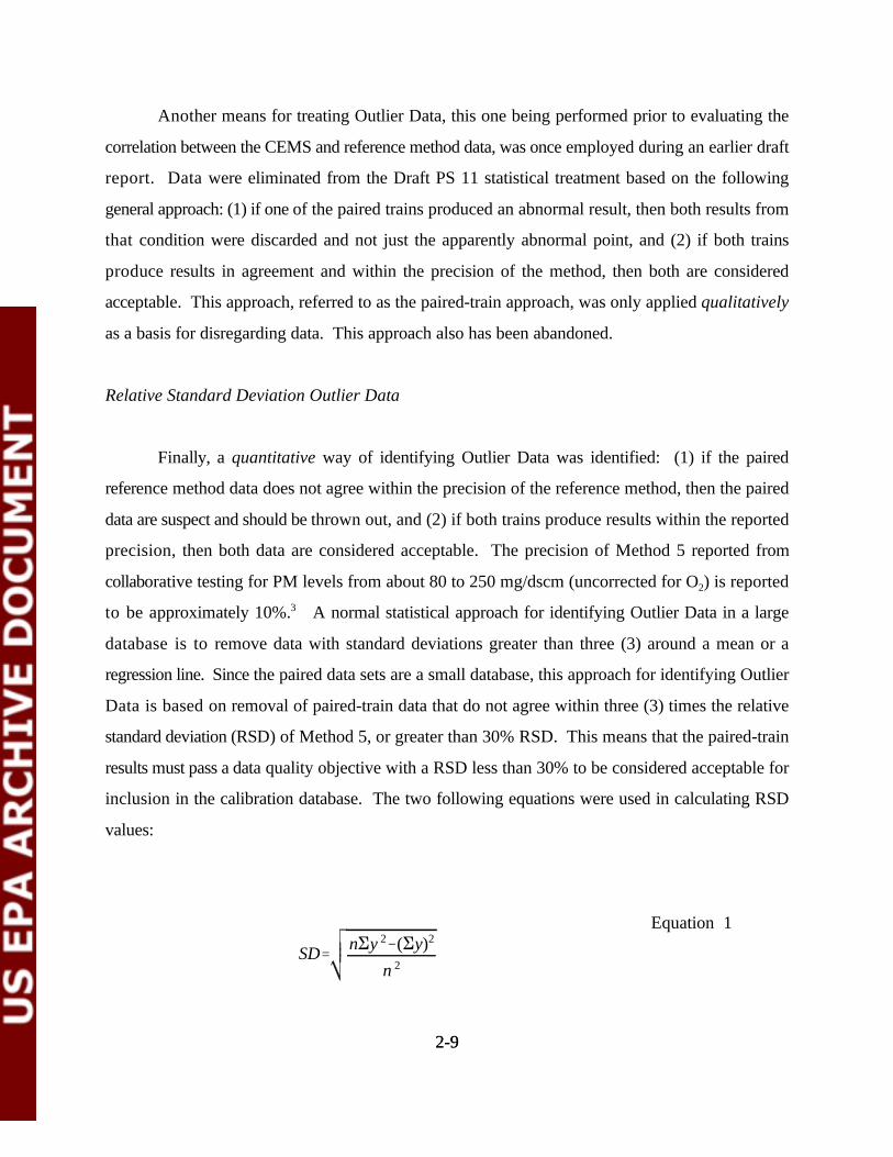
Finally, a quantitative way of identifying Outlier Data was identified: (1) if the paired

reference method data does not agree within the precision of the reference method, then the paired

data are suspect and should be thrown out, and (2) if both trains produce results within the reported

precision, then both data are considered acceptable. The precision of Method 5 reported from

collaborative testing for PM levels from about 80 to 250 mg/dscm (uncorrected for O ) is reported2

to be approximately 10%. A normal statistical approach for identifying Outlier Data in a large3

database is to remove data with standard deviations greater than three (3) around a mean or a

regression line. Since the paired data sets are a small database, this approach for identifying Outlier

Data is based on removal of paired-train data that do not agree within three (3) times the relative

standard deviation (RSD) of Method 5, or greater than 30% RSD. This means that the paired-train

results must pass a data quality objective with a RSD less than 30% to be considered acceptable for

inclusion in the calibration database. The two following equations were used in calculating RSD

values:

Equation 1

RSD SDM

X 100%

2-102-10

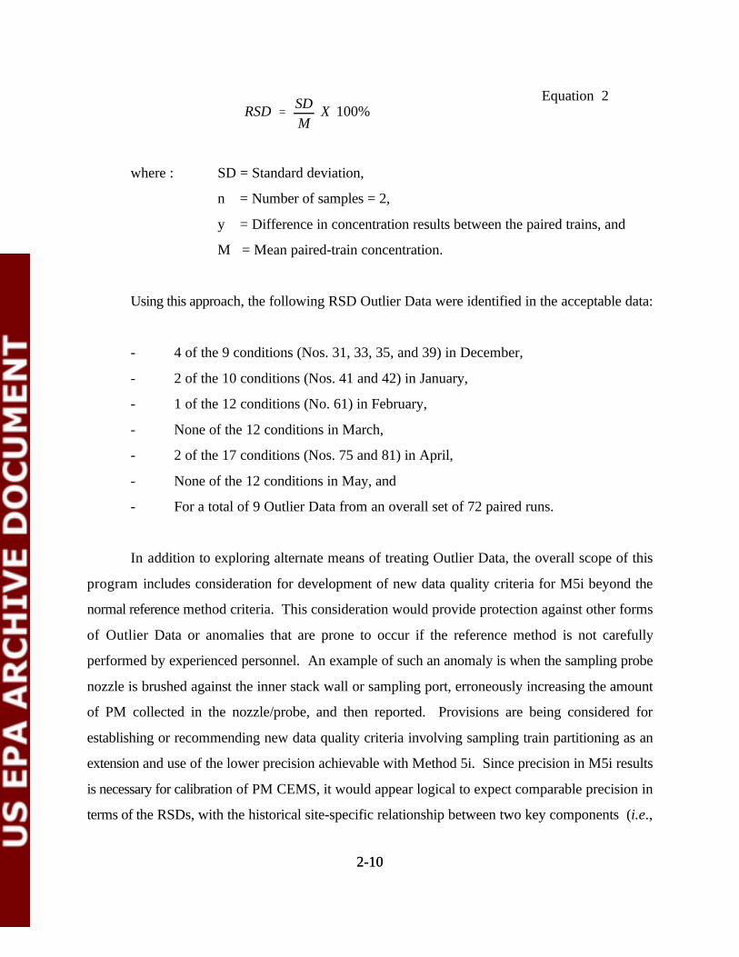
Equation 2

where : SD = Standard deviation,

n = Number of samples = 2,

y = Difference in concentration results between the paired trains, and

M = Mean paired-train concentration.

Using this approach, the following RSD Outlier Data were identified in the acceptable data:

- 4 of the 9 conditions (Nos. 31, 33, 35, and 39) in December,

- 2 of the 10 conditions (Nos. 41 and 42) in January,

- 1 of the 12 conditions (No. 61) in February,

- None of the 12 conditions in March,

- 2 of the 17 conditions (Nos. 75 and 81) in April,

- None of the 12 conditions in May, and

- For a total of 9 Outlier Data from an overall set of 72 paired runs.

In addition to exploring alternate means of treating Outlier Data, the overall scope of this

program includes consideration for development of new data quality criteria for M5i beyond the

normal reference method criteria. This consideration would provide protection against other forms

of Outlier Data or anomalies that are prone to occur if the reference method is not carefully

performed by experienced personnel. An example of such an anomaly is when the sampling probe

nozzle is brushed against the inner stack wall or sampling port, erroneously increasing the amount

of PM collected in the nozzle/probe, and then reported. Provisions are being considered for

establishing or recommending new data quality criteria involving sampling train partitioning as an

extension and use of the lower precision achievable with Method 5i. Since precision in M5i results

is necessary for calibration of PM CEMS, it would appear logical to expect comparable precision in

terms of the RSDs, with the historical site-specific relationship between two key components (i.e.,

2-112-11

probe rinse and filter weight gains) forming the end result.

2.3 Facility Operation Summary

The incinerator operated in a manner to maintain the facility at or below the permitted levels

and to accommodate the calibration relation tests as much as possible. The PM CEMS calibration

tests for this demonstration program were conducted in accordance with Draft PS 11 protocol and

within the terms of the agreement with the site facility. Given these constraints and goals, the

calibration tests were conducted under a wide variety of incinerator waste feedstream and air

pollution control (APC) conditions across the facility’s normal PM emission range. Keep in mind that

the rationale for selection of this test site was to present a worst-case challenge to the PM CEMS due

to its inherent diversity of operating conditions potentially affecting PM CEMS performance. This

aspect of diversity was realized since there were several deliberate and inadvertent changes with

respect to facility operating conditions during the calibration test periods. The facility conditions that

changed due to seasonal and normal operating variations include:

1) No constraints or reproducibility on the wide variety of waste feedstreams,

2) Variations in equipment operating and maintenance conditions, and

3) Measurable variations in the stack gas conditions in terms of PM concentration

and composition, temperature, moisture, diluent concentration, and gas flow rate.

2.3.1 Facility Operation During the Two Calibration Relation Tests

Two (2) calibration relation tests were performed under a similarly wide variety of facility

operating conditions. These operating conditions covered the full range of operations at the facility,

which in turn caused changes in PM properties and emission levels. The calibration testing in

December through March was intended to establish the (initial and only) calibration relation for each

CEMS relative to the reference method. As experience was gained, data quality improved, and as

a result of comments received from the first CEMS NODA, it was decided that a second calibration

2-122-12

relation test be conducted in April to evaluate the stability of the PM CEMS relations. The calibration

relation tests were again performed in accordance with Draft PS 11.

Facility Operation During First Calibration Relation Test

The calibration relation testing for this demonstration required an attempt to generate wide

variations in PM emission properties (such as composition, size distribution, density, and color), PM

emission concentration levels, and in flue gas conditions (such as temperature, moisture, diluent

concentration, and gas flow rate). Table 2-1 presents the matrix of planned test conditions. For

characterizing PM CEMS performance under normal operations, testing was conducted under as-

found facility operations during one-week periods from December to March. To collect data over

the incinerator’s entire range of PM emissions, it was necessary to continue until high PM levels were

produced in March. Six (6) types of fuels and/or wastes in at least nine (9) different combinations

were fed to the incinerator over three (3) EDV power settings for a total of 36 test conditions. The

six (6) waste/fuel types fed to the primary combustion chamber were:

1) Fuel oil;

2) Solids (including shredded paper, animal bedding, and office/laboratory waste);

3) High-chlorinated solvents (e.g., ortho-dichlorobenzene, carbon tetrachloride);

4) A mixture of low- and/or non-chlorinated solvents (e.g., acetone, acetonitrile, butanol,diethylamine, dimethylacetamide, ethyl acetate, hexane, hexamethylenediamine,hydroxyethylidene, isopropanol, methanol, methylene chloride, methyl ethyl ketone,toluene, or xylene);

5) Paint pigments (containing water, resins, and solvents); and

6) Jugs (containing non-, low-, or high-chlorinated solvents).

PM-related process data from the plant records were collected to document the range of

plant operation covered during calibration testing. These data were also collected to allow evaluation

2-132-13

of operating condition effects on PM emission levels or CEMS performance. Waste availability

determined the order and accounted for the random sequence of the test conditions.

PM-related APC equipment performance was not deliberately varied except for the EDV

power levels. The EDV power was adjusted with a programmable logic controller for three (3) set

points: 0.2 - 0.3 kW for the low power, 1.0 kW for the mid-power, and 2.0 kW for the high power

conditions. Another key, but not-so-controllable, variable affecting PM emission characteristics is

the contribution from solids in the recycled scrubber water injected into the spray dryer. The

incinerator’s elevated temperature exhaust gas evaporates the recycled scrubber water injected into

the spray dryer for removal of dissolved and suspended solids collected by the wet scrubbers. Metals,

salts, fly ash, and unreacted soda ash (sodium carbonate for pH control) make up the dissolved and

suspended solids carried in the scrubber water ultimately removed as dry PM material in the spray

dryer and cyclone. Since a hysteresis effect tends to occur from the scrubber water solids, its

contribution of PM emissions is not subject to direct, immediate control of affecting PM emission

levels. And because of their fixed design configurations, none of the PM-related performance

parameters of the spray dryer, cyclone, or venturi scrubber could be deliberately varied.

A general summary of the facility operating data for each condition in the first calibration

relation testing is presented in Table 2-2. Records with a more detailed account of the facility

operating data during testing are included in the Appendix.

Facility Operation During Second Calibration Relation Test

The second calibration relation test was conducted in a manner similar to, but not exactly

duplicative of, the first one. The general nature of the incinerator operating conditions and waste feed

combinations of the first calibration relation test was similar to the second test. Comparison

of the waste/fuel type combinations fed between the first and second tests are shown in the following:

2-142-14

First Calibration Second Calibration

1) Mixed solvents and solids 1) Mixed solvents and solids

2) Chlorinated solvents and solids 2) Mixed solvents, chlorinated solvents and solids

3) Mixed solvents, solids, jugs, pigments 3) Mixed solvents, solids, jugs, and pigments

4) Mixed solvents 4) Mixed solvents

5) Mixed and chlorinated solvents 5) Mixed and chlorinated solvents

6) Mixed solvents, solids, jugs 6) Mixed solvents, solids, and pigments

7) Mixed solvents, solids, jugs

8) Chlorinated solvents, solids, jugs

9) Fuel oil and solids

However, the PM emission range of the second calibration relation test was lower than the

first test. This probably was the result of greater PM removal from higher EDV power levels: 1.0

kW for the low power, 2.0 kW for the mid-power, and 3.0 kW for the high power conditions.

Though the intent was to simulate waste-feed types and PM emission loadings, there were at least

three (3) other factors that precluded exact duplication of facility operating conditions and PM

emission levels:

1) The normally wide variety of wastes and feedstream combinations meant the exact same feed

materials were not available;

2) The hysteresis effect of recycling scrubber water back to the spray dryer meant that the

amount and type of PM evaporated from the scrubber water could not be reproduced; and

3) Incinerator operational constraints.

Recall that this particular facility was chosen because it treats a very broad assortment of waste

feedstocks, most in small quantities. While this is desirable from a worst-case PM CEMS challenge

One aspect of the test was to ascertain the achievability of the Draft PS 11 and data quality objectives8

themselves. As a result, some improvements in the approach were made as EPA learned how to better conduct the tests. This includes EPA’s decision to have 12 tests represent an RCA, the decision that an RCA is to be conducted under"normal" operations over the same PM emission range as the calibration test, and the current proposed specification

2-152-15

standpoint, these aspects did not allow reproducing the identical feed, operating conditions, and PM

emissions that were obtained in the first calibration tests. Table 2-2 also presents a general summary

of the operating data for each condition in the second calibration relation testing with a more detailed

account of the facility data included in the Appendix.

2.3.1 Facility Operation During RCA Testing

The final monthly test in May 1997 was considered a RCA and performed under as-found

facility conditions to represent normal day-to-day operations. No attempts were made to control the

waste-feed streams for this test, although EDV power set points were adjusted to three (3) different

levels: 1.0 kW for the low power, 1.5 kW for the mid-power, and 3.0 kW for the high power

conditions. Similar to the calibration tests, the normal variety of waste feedstreams were added

during the May monthly test. The feedstreams included the same types of waste streams as in the

calibration tests along with additional types, combinations, and/or relative feed rate distributions of

solids, mixed solvents, chlorinated solvents, jugs, pigments, and fuel oil. Likewise the changes in

EDV power settings gives the same appearance of a similarly irregular pattern overlaying the

feedstream diversity. This heterogeneous array of feedstreams and EDV power levels reflect a

random configuration of test conditions portraying usual day-to-day operations. Table 2-2 also

presents a general summary of the operating data for each condition in the May test. A more detailed

account of the facility data is included in the Appendix.

Facility operations during the September through November 1996 tests also reflected

incinerator conditions, waste feedstreams, and EDV power levels similar to the calibration tests.

Despite the merits cited, the monthly tests were not always performed in strict accordance

with the Draft Appendix F - Procedure 2 requirements for RCA tests. The structure and results of8

levels. Obviously since the approach was updated as the program progressed, the RCA tests themselves might notexactly conform to what was proposed. This reflects the evolutionary nature of these tests.

2-162-16

these tests did not completely meet one of the following two important criteria for RCA tests: either

1) operating the facility across the same PM emission range as the calibration test, or 2) testing at

three or more different PM concentrations for a minimum of twelve (12) measurement sets.

However, combinations of two/three months or the overall collection of monthly tests do meet the

RCA testing criteria.

2.3.2 Summary of Facility Operation Over the Test Program

Facility operation over the test program is summarized by the following achievements:

Under reasonable worst case (as-found, normal day-to-day) HWC facility operations,

Consisting of various conditions with waste feeds, APC performance, PM, and flue gas,

Across a 9-month and 4-seasonal period, and

During a total of two (2) calibration relation tests and four (4) RCA tests.

In regard to trends, there were measurable variations in the stack gas conditions in terms of

temperature, moisture, diluent concentration, and gas flow rate. These seasonal trends and typical

variations, coupled with ordinary day-to-day operations, attest that the facility conditions over the

course of the test program indeed were representative of regular operations at a HWC incinerator.

2.4 CEMS Calibration Relation Test Results

The scope of this subsection focuses on the results produced during the first and second

calibration tests in relation to Draft PS 11. These results form the basis on which each CEMS

calibration is established and then evaluated in terms of the three data acceptance criteria specified

in the revised Draft PS 11. The results from the two calibration relation tests are independently

2-172-17

calculated and evaluated, and then any similarities/differences between the two (2) sets of results are

characterized. All data are presented, but the Draft PS 11 statistical evaluations are performed on

only acceptable data meeting the QA objectives. Clarifications are included to account for the

rationale and the details involving treatment of data.

Two (2) calibration relation tests were performed under a similarly wide variety of facility

operating conditions to establish the correlation between the reference method and the output of each

respective monitors. The calibration test in December through March was intended to establish the

(initial and only) calibration for each CEMS relative to the reference method. Due to a narrow range

of PM produced in the December through February tests, four (4) separate periods were needed to

complete the first calibration. A second calibration test was conducted the following April to evaluate

the reproducibility of the data quality produced not only from the PM CEMS but also from the

reference method. Both calibration tests were conducted largely in agreement with Draft PS 11

consisting of these main elements:

1) The facility operated across its normal PM emission range and beyond/near the highest

proposed PM emission standard (69 mg/dscm);

2) Sets of PM CEMS and manual reference method measurements were simultaneously

obtained; and

3) These tests were performed at three (3) or more PM concentrations for a minimum of 15

measurement sets.

Exceptions/deviations in meeting the above criteria included:

1) The range of acceptable data for the ESA Beta monitor only rose to about 80% of the

Due to setup for a lower PM range up to 50 mg/acm, the ESA monitor produced over range flagged data for9

the three highest PM runs (Nos. 65, 66, and 67) in the second calibration test. The monitor is equipped to measure PMup to 4,000 mg/acm, but was adjusted for measuring the normal facility levels below 50 mg/acm, which caused point 1to occur.

The automatic span calibration checks for the Durag monitor showed deviations from the reference value10

up to 8% during the March calibration relation tests, which caused point 2 to occur.

2-182-18

proposed 69 mg/dscm standard in the first calibration test, 9

2) The automatic internal span calibration check recorded on the DAS failed to meet the

specification limit for the Durag monitor throughout the second calibration relation tests,

resulting in its test data to be considered invalid, 10

3) The range of PM emissions, and of the monitors’ responses, only rose to about 80% of

the proposed 69 mg/dscm standard in the second calibration relation test.

Reference Method 5 PM Results. Both sets of the calibration relation results of the M5i

measurements for each train are shown in Table 2-3 with the PM concentration results expressed in

actual and dry standard units along with their respective temperature and moisture content values.

The average PM concentration and RSD results are also presented in Table 2-3. All supporting data

and records are contained in the Appendix. The PM results produced from M5i ranged from about

5 to 75 mg/dscm at 7% O and from about 5 to 55 mg/dscm at 7% O during the first and second2 2

calibrations, respectively. Results are reasonably distributed across the range of PM concentrations

developed in both the first and second calibration relation tests. All runs produced results with RSDs

less than 30% except for 7 of the 43 runs in the first calibration and 2 of the 17 runs in the second

calibration that were considered Outlier Data. Most of the weight gain was associated with the filter

catch, as there was generally 5 to 25 mg weight gain on the filters and 0.5 to 4 mg weight gain from

the front-half probe rinses.

CEMS PM Results. Results produced from each CEMS for each test condition during the

2-192-19

calibrations are presented in Table 2-4. These were developed from averaging the 1-minute CEMS

records collected on the data logger for the corresponding M5 sampling times, excluding the times

during port changes. Data from the ESA and Verewa Beta monitors were offset corresponding to

their response times.

Careful review of each CEMS data was also performed. This involved checking data recorded

by the data acquisition system (DAS) relative to corresponding Method 5 sampling times along with

consideration of respective response time offsets for the two (2) Beta monitors. Since several CEMS

were undergoing PM calibration testing as a set of individual monitors (and not just one), the policy

was to proceed with testing even though one (1) or more of the CEMS were not operating properly

or experiencing internal calibration. Records and DAS data were also examined to determine if each

CEMS was functioning properly, calibrating within specifications, or going through an internal

automatic calibration, during the test period. Although this type of check is obvious and

straightforward for one (1) CEMS of a proven and familiar technology, it is not necessarily so for

multiple CEMS which are undergoing demonstration and consequently represent not-so-familiar

technology.

The CEMS data review showed that there were calibration test periods in which the monitors

produced invalid data during a portion of or throughout the entire run. For a run to be considered

acceptable, a criterion for a minimum time of 80% data availability for each test condition was

developed. This means that if any of the CEMS was out of commission (i.e., not operating properly

or experiencing internal calibration) for more than 20% of the total testing period, the CEMS data

for that run was considered invalid. The one minute-average data recorded by the DAS was applied

as the basis of the data availability percentage calculation for the test periods.

As a result of the QA audit, it was determined that the following four (4) CEMS were not

operating properly, producing suspect data, or were experiencing calibration during the following test

conditions in the calibration tests:

For example, the three (3) light-scattering monitors and the ESA Beta monitors perform their analysis under11

actual in-stack conditions, and thus produce PM concentration data proportional to that reference; whereas, the Verewameasures the sample gas volume under dry conditions and then calculates the PM concentration to a (dry) standardreference temperature.

2-202-20

CEMS Test Month: Run Number Rationale

ESA January : 48 Data were outside the set range (footnote 6).

March : 65, 66, 67 Data were outside the set range (footnote 6).

April : 83, 87, 88 Change in velocity, unable to maintain isokinetic sampling.

May : 98 Change in velocity, unable to maintain isokinetic sampling.

Verewa January : 41, 42, 44, 49 Off-line due to a mechanical failure.

May : 91, 92, 93 Off-line due to a mechanical failure.

Durag January : 42 Monitor in zero mode.March : 62 to 73 Internal span calibration check failure.

Sigrist May : 92, 93 Off-line due to blower failure.

DRAFT PS 11 Calibrations. The statistical calculations for the two (2) calibration tests were carried

out according to the equations and definitions in Draft PS 11 for the correlation coefficient,

confidence interval, and tolerance interval. These involved performing a regression analysis on the

correlations between paired set of CEMS and M5i data over corresponding time periods. Depending

on the measuring conditions experienced by the individual monitors, the PM CEMS data are

correlated with the corresponding M5i results presented in either actual in-stack (mg/actual cubic

meter (acm) or dry standard concentration units (mg/dscm). Three (3) mathematical approaches11

are available for evaluation to determine which approach provides the best fit to the calibration data.

These approaches include:

Linear relation,

Quadratic relation, and

2-212-21

Logarithmic relation.

A linear calibration relation is calculated by performing a linear least squares regression. The

CEMS data are taken as the x values and the reference method data as the y values. A linear

calibration relation, which gives the predicted PM concentration, y’, based on the CEMS response

x, is given by:

y’ = a*x + b

where :

a = slope of the linear regression line, and

b = y intercept.

A quadratic calibration relation is calculated by performing a second-order least squares

regression. Similarly, the CEMS data are taken as the x values and the reference method data as the

y values. A quadratic calibration relation, which gives the predicted PM concentration, y’, based on

the CEMS response x, is given by:

y’ = b *x + b *x + b2 1 02

where :

b = coefficient for the first term of the quadratic equation,2

b = coefficient for the second term of the quadratic equation, and1

b = y intercept.0

A logarithmic calibration relation is calculated by substituting x = log x, and then by

performing a linear least squares regression on the logarithmic values of x. The log of the CEMS data

are taken as the x values and the reference method data as the y values. A logarithmic calibration

relation, which gives the predicted PM concentration, y’, based on the log x of the CEMS response

x, is given by:

2-222-22

y’ = a *(log x) + b3 3

where :

a = slope of the linear regression line for log x, and3

b = y intercept.3

The rationale and benefits of applying a logarithmic relation to fitting certain calibration data are

discussed in the context of performing the PS 11 statistical evaluation in the following subsection.

Following this, the 95% confidence interval for the regression relation is computed, as is a

tolerance interval, which predicts the bounds of 75% of the population of the manual method data

with 95% confidence. Both intervals would normally be calculated at the emission limit, but for this

program, both intervals are determined at each of the three (3) proposed emission limit levels (i.e.,

69, 50, and 34 mg/dscm @ 7% O ). The equations provided in Draft PS 11 were put on a2

spreadsheet, while values for t , v , and u ’ were automatically inserted from Table I in Draft PS 11;f f n

for the logarithmic correlations, the series of equations to calculate the confidence and tolerance

intervals were performed by substituting x = log x in the linear calibration relation equations. In

essence, the confidence interval predicts the bounds in which one would expect any calibration line

to lie, with 95% confidence, if other CEMS and manual method data from the same population as

those observed during the calibration test were used. The tolerance interval bounds the region within

which one would expect 75% of other manual method and CEMS data to fall, with 95% confidence,

based on the CEMS and manual method measurements observed during the calibration.

Before discussing the calibration results, two clarifications are in order concerning the

methodology of the CEMS performance evaluations applied in this program and those relevant to

future certifications performed by industry. First, for the purpose of this demonstration program,

there is a total of seven (7) data acceptance criteria used to evaluate CEMS performance. These are:

a) the correlation coefficient (at one level, as it is calculated independent of emission limits),

b) three (3) confidence interval measures (at each of three proposed emission limits), and

2-232-23

c) three (3) tolerance interval measures (at each of three proposed emission limits).

In future CEMS certifications performed by industry, there would only be three (3) acceptance

criteria. For the second clarification, since the calibration range, or its regression equation, did not

always reach each of the three (3) proposed limits, then the maxima of the calibration or the

regression equation is applicable and used as the reference emission value upon which the evaluation

of the confidence and tolerance intervals is performed. This procedure would also be applicable in

future CEMS certifications.

First and Second Calibration Relation Results Based on Linear Fit Approach

The first calibration test results of the Draft PS 11 linear relation statistical calculations are

presented in Table 2-5 for all five (5) CEMS. Table 2-5 lists the revised Draft PS 11 data acceptance

criteria for the correlation coefficient, confidence interval, and tolerance interval as well as presents

the results of these criteria relative to the three (3) proposed PM emission limits for each of the two

(2) calibrations for each monitor. For the first calibration relation data set, each of the five (5)

CEMS, with one minor exception, produced data meeting the revised PS 11 criteria at all three (3)

proposed PM emission limits based on a linear approach for fitting data: correlation coefficient

criterion of greater than 0.90, confidence interval less than 10%, and tolerance interval less than

25%. Despite meeting six of the seven criteria, the Sigrist did not achieve the tolerance interval

measure at the lowest emission standard. Note that although the Durag produced acceptable data

over 95% of the time, it was not operating properly, according to its self-calibration span check

report, during the March calibration tests with the highest measured PM levels. Consequently, it

reflects a more narrow range over which the initial calibration was performed. Figures 2-1 through

2-5 then graphically illustrate the linear regression lines for each set of calibration data pertaining to

the ESA, Verewa, Durag, ESC, and Sigrist monitors, respectively.

The second calibration test results of the Draft PS 11 linear relation statistical calculations

are also presented in Table 2-5 for all five (5) CEMS. For the second calibration relation data set,

2-242-24

the same four (4) CEMS (ESA, Verewa, Durag, and ESC) produced data which met all seven (7) of

the PS 11 criteria applied in this program. The Sigrist monitor met five of the seven criteria, but did

not produce data meeting the confidence interval at the 50 mg/dscm standard or at the maximum of

the calibration range. Figures 2-1 through 2-5 also show graphical representations of the second

calibration’s linear regression line for the ESA, Verewa, Durag, ESC, and Sigrist monitors,

respectively.

Review of the comparison between the two (2) calibration relation linear regression lines and

their corresponding equations in Figures 2-1 through 2-5 give insight into three important aspects of

these two (2) calibration relation tests:

1) Reproducibility, or stability, of CEMS performance in terms of the equations defining their

linear relationship with M5i measured results;

2) Reproducibility in data quality associated with the M5i results produced in the first and

second calibration tests, and

3) If there is non-reproducibility between the two (2) linear regression lines in a linear fit

approach, then further actions are necessary to examine either potential causal factors

(e.g., test procedures, sampling location, change in PM properties) or non-linear approaches

in fitting CEMS data reproducibly with M5i measured results.

For the first point on CEMS performance, the equations defining the linear regression of each

calibration would agree despite differences in time and test operating conditions if a) the calibration

relationship were stable over time, b) insensitive to changes in PM properties, and c) insensitive to

differences in PM range over which the calibration was performed. Comparison of the slopes of the

linear equations is considered to be the definitive measure in this comparison, since all y-intercepts

in the equations have nominal values of 5 (mg/acm or mg/dscm) or less. The tabulated data below

presents a comparison of the two calibration linear equations’ slopes for each CEMS. Relative to

Percent Difference in slope = |s -s ]/s x 100%.12i AVG AVG

2-252-25

a linear fit approach, this comparison shows agreement within 4% for the two (2) Beta monitors and

within 7% for the Durag light-scattering monitor. This level of agreement reflects acceptability of

subsequently applying a linear regression for the ESA, Verewa, and Durag monitors over time, over

their respective PM ranges, and over these operating conditions (variations in waste feedstreams, PM

properties, and flue gas conditions).

CEMS First Calibration Slope Second Calibration Slope % Difference12

ESA 0.824 0.766 3.6

Verewa 1.343 1.430 3.1

Durag 0.421 0.366 6.9

ESC 0.357 0.448 11.3

Sigrist 0.199 0.313 22.2

Regarding the second aspect on M5i results, duplication in the data quality from the M5i

results between the two (2) calibration tests is reflected, given nearly identical reproducibility in

performance with three independently operating CEMS, with nearly identical correlation coefficients,

confidence intervals, and tolerance intervals. Since a high degree of correlation and reproducibility

is indirectly confirmed from data produced by three (3) of the CEMS using a linear fit approach, this

establishes that duplication in the data quality from the M5 results occurred between the two (2)

calibrations.

Relative to the third point on the non-reproducibility from a linear fit approach, it is consistent

with Draft PS 11 and ISO 10155 protocols to evaluate alternative non-linear calibration relation and

identify one which best fits the data. Since the possibility of M5i-related causal factors is eliminated

and the 11 to 22% variation in the ESC and Sigrist linear regression line slopes is unacceptable, other

testing-related factors for non-reproducibility or non-linear approaches for finding a best fit approach

need to be investigated. Discussion of the investigation regarding other factors and non-linear

2-262-26

approaches follow.

Further Investigation Into Linear Fit Approach for Light-scattering CEMS

The results of further analysis to address the effect of the calibration range on the regression

line slopes developed from the two (2) calibrations for the ESC and Sigrist light-scattering CEMS

are presented in Table 2-6. Recall that the initial calibration traversed a higher range than the second

calibration, as the highest PM levels measured in the program occurred in March. Further analysis

indicates a profound effect of the range over which calibrations are performed and clearly

demonstrate the criticality of high-end PM data. This effect is shown in Table 2-6 which indicates

stability (< 2% difference) between the two (2) calibrations for the Beta and light-scattering CEMS

as the March data are commonly included in both calibrations (see Column A/D). This is due to the

slope-setting nature of the end-point data on defining the regression line with scatter in the low-end

PM data. However, even by rearranging the March data with the second calibration data set instead

of the first, there is still an unacceptable 22% and 34% variation in the ESC and Sigrist linear

regression slopes, respectively, between the two (2) “rearranged” calibrations (see Column C/D).

In summary, this analysis on the effect of the calibration range does suggest the importance of high-

end PM data but does not explain why the ESC and Sigrist light-scattering CEMS produce dissimilar

linear regression lines for the two (2) original and rearranged calibrations data sets, whereas the Beta

monitors do (see Columns A/B and C/D).

Evaluation of Non-linear Fitting Approaches For Light-scattering CEMS

Since linear regressions do not provide a suitable fit for the ESC and Sigrist light-scattering

CEMS, still further analysis is warranted to evaluate whether non-linear approaches are applicable

in defining the same, reproducible relationship for both sets of calibration data. Following are such

analyses assessing the fit between the two (2) calibration sets with a quadratic relation and then a

logarithmic relation.

2-272-27

A quadratic regression was developed using a least-squares approach for determining the

coefficients in a second-order equation for the ESC and Sigrist light-scattering CEMS. Figures 2-6

and 2-7 graphically illustrate the quadratic regressions fitting each of the two (2) calibrations for the

ESC and Sigrist CEMS, respectively. As seen in both figures, quadratic regressions may fit the

individual calibration data adequately, but produce 1) two dissimilar equations for each calibration,

and 2) equations with inadmissible characteristics in that there is a range of data with a positive slope

followed by a negative slope. The first point reflects the same non-reproducibility shortcoming

associated with the linear regression approach, while the second point depicts the monitors as not

being monotonic (i.e., producing two different responses for the same PM concentration). As a result

of each of these limitations, the quadratic regressions do not provide usable fits for the ESC and

Sigrist light-scattering CEMS calibration data obtained from the test site facility.

A logarithmic regression was developed using a least-squares approach for the ESC and

Sigrist light-scattering CEMS. This was accomplished by using the exact same equations as in the

linear regression but with substitution of log x (base 10) values for the x values (x values = CEMS

readings). Figures 2-8 and 2-9 graphically illustrate the logarithmic regressions fitting each of the

two calibrations for the ESC and Sigrist CEMS, respectively. As seen in these two figures,

logarithmic regressions not only fit the data very well, but produce 1) two near-identical equations

for each calibration (agreement within about 2%), and 2) equations with admissible characteristics.

The first point reflects a solution to the non-reproducibility barrier associated with the linear and

quadratic regressions, and the second point depicts the monitors being monotonic (i.e., producing one

unique response for each PM concentration).

Because of the acceptable fit of the logarithmic regressions, the remaining statistical

calculations for the Draft PS 11 data acceptance criteria were performed on the two (2) calibration

data sets for the ESC and Sigrist light-scattering CEMS. This was likewise accomplished by using

the exact same equations as in Draft PS 11 for linear calibration relations but with substitution of

log x values for the x values. Table 2- 7 presents the results for the Draft PS 11 data acceptance10

criteria based on logarithmic regressions. These same results are graphically illustrated in Figures 2-8

2-282-28

and 2-9 for the ESC and in Figures 2-10 and 2-11 for the Sigrist for each of the two (2) calibrations,

respectively. The results produced by the ESC meet all three (3) revised PS 11 data acceptance

criteria at all three (3) levels near/at the proposed PM limits for both calibrations. The Sigrist-

produced results meeting six (6) of the seven (7) criteria in the first calibration, but only met four (4)

of the seven (7) criteria during the second calibration.

These data indicate that the logarithmic performance of the ESC and Sigrist light-scattering

CEMS is attributable to a shift to a smaller particle size distribution (PSD) as PM concentrations

increase. This is logically explained by the following:

1. The amount of light scattered is proportional to the surface area of the particles;

2. For a matrix of any PM concentration, there is a given surface area for a given PSD and a given amount of light scattered;

3. As PM concentration changes with the same PSD, then the amount of light scattered is linearly proportional with incremental changes in PM concentration;

4. A PM matrix with a smaller PSD will produce higher incremental changes in light scattered relative to the same given change in PM concentration for a larger PSD PM matrix;

5. For the case when PM concentration increases with an accompanying shift to a smaller PSD, then the relative amount of light scattered per unit of PM concentration increases;

6. Conversely, for the case when PM concentration increases with an accompanying shift to a larger PSD, then the relative amount of light scattered per unit of PM concentration

decreases;

7. At the facility tested, it is believed that elevated PM stack concentrations were associatedwith a shift to a smaller PSD, caused either by a) reduced collection performance of thepolishing APC device on small sized PM, and/or b) higher concentrations of small sized PMpenetrating the venturi scrubber and the polishing APC device.

The PSD data of the facility’s PM emissions produced during the test program show a high

concentration of small particles ( < 2.0 microns) with a mean particle size of about 0.5 microns and

about 85% of the PM less than 2.0 microns (see Section 2.6.7 for more discussion on PSD results).

2-292-29

Such a high concentration of small-sized PM is consistent with facility-measured PSD data and other

data on similarly equipped facilities with a venturi scrubber. This should not be construed as a

conflict with other data supplied by light-scattering vendors on other industries and APC

technologies with accompanying particle size distributions. These other data show that the

regression correlation is linear for PM concentrations up to (about) 100 mg/acm, and that the nature

of the regression changes to a quadratic relation at that point. Since this has been demonstrated that

this “break” in the relation is related to the behavior of the APC as well as the PSD, these data do not

conflict. Rather they show results that are relative to the process and APC configurations tested.

Further, they substantiate the fact that this “break” can be anticipated to shift based on the process

and APC configuration being evaluated. Thus, it is expected that linear and quadratic fits are

applicable for other types of APC technologies on HWC facilities as well.

2.5 CEMS RCA Test Results

This section focuses on the results produced from these demonstration tests in relation to

RCA criteria specified in revised Draft PS 11. RCA tests are used to determine whether the

calibration is still valid, i.e., whether CEMS performance varied over time. Due to the non-

reproducibility of waste feedstreams, the monthly tests also furnish a measure of evaluating CEMS

reproducibility despite variations in PM properties and flue gas conditions. Results from monthly

testing as well as the overall collection of test results are independently calculated and evaluated

based on RCA criteria relative to each of the two (2) calibrations. Subsequent RCA measurements

comparing CEMS responses to reference method data are considered consistent with the current

calibration relation if at least 75% of them fall within a tolerance level of 25% calculated at the PM

emission standard. All data are presented, but the RCA evaluations are performed on only acceptable

data meeting the QA objectives. Clarifications are made when data are not used in the RCA

evaluations.

Recall that most of the individual monthly RCAs were not performed in strict accordance with

all Appendix F - Procedure 2 requirements. This was due to the developmental nature and learning

2-302-30

process involved as well as the lack of influence to override normal operations in controlling waste

feedstreams and the range of PM concentration for calibration test purposes. The structure and

results of most monthly tests did not meet the following two (2) RCA test requirements:

1) The facility was operated across its normal PM emission range with assurance that all

measurement sets are collected within the same range as in the calibration test, and

2) Testing was not performed at three (3) or more PM concentrations and at least 12

measurements were not always taken. Some earlier monthly tests only contained nine or ten

conditions and many did not consist of three (3) or more PM stack concentrations, as was the

case in the calibration relation test.

However, data produced in each monthly test does address the key issue of CEMS reproducibility

performance over time, and the overall set of monthly data collectively meet the RCA criteria. The

collective body of test results also serve an additional purpose of providing supporting data for each

PM CEMS by forming an overall cumulative database. This cumulative database includes all valid

test data, including the May monthly test results and the two calibrations, but without the September

through November data.

Reference Method 5 PM Results. All M5i measurements from the May test for each train are shown

in Table 2-3 with the PM results expressed in actual and dry standard units and in their respective

temperature and moisture values. The average PM and RSD results are also presented in Table 2-3.

The supporting data and records are contained in the Appendix. The PM results produced from M5i

ranged from about: 5 to 75 mg/dscm at 7% O for all the tests from December to April, 5 to 452

mg/dscm at 7% O for the May test, and 10 to 100 mg/dscm at 7% O for the September through2 2

November tests. Many of these results were concentrated in the low range. The test runs with RSD

Outlier Data were specified earlier, as there were no Outlier Data in the May test.

CEMS PM Results. Results produced from each CEMS for each test condition during the monthly

This revised RCA evaluation procedure is based on the calibration relation regression line and the +/- 25%13

tolerance interval criteria, but is independent of the tolerance interval calculated from the calibration test; as such, it isdistinct from, and not to be confused with, the data-dependent tolerance interval approach used in the calibration relationevaluation.

2-312-31

tests are presented in Table 2-4. CEMS data from each run were carefully reviewed to ensure the

CEMS was properly operating during a given run. From CEMS data review, it was determined that

certain monitors were not operating properly, producing suspect data, or were experiencing

calibration during the test conditions as specified earlier.

Evaluation of RCA Results. The RCA results are compared to the calibrations to determine if the

calibration is still valid. If at least 75% of the manual method data collected during an RCA fall

within the 25% tolerance intervals, then the calibration is still considered valid. If less than 75% of

the data fall within the tolerance interval, then the calibration is considered no longer valid and a

recalibration is necessary.

The following explanation, along with the accompanying tables and figures, illustrates the

revised Appendix F - Procedure 2 procedure and principles to evaluate acceptability of the subsequent

RCA data relative to the calibration relation. First, a figure is produced showing the calibration13

relation regression line based on the calibration data and the tolerance intervals set at +25% of the

PM emission standard. The tolerance interval bounds an area on the graph, +25% of the numerical

emission limit from the calibration regression line on the y-axis, traversing across the calibration range

(from the lowest to the highest CEMS output reading of the calibration) on the x-axis. Second, the

paired CEMS/M5i values from the RCA tests are plotted and overlaid onto the figure just described.

Finally, the number of points that are visually apparent to be inside the tolerance intervals are

counted. For data points falling on the tolerance interval boundary line, it will be necessary to

numerically determine whether the RCA data are within the boundaries by calculating the tolerance

interval value and comparing it to the coordinates of the specific RCA data point on the line. If at

least 75% of a minimum of the twelve RCA points fall within the tolerance interval and the calibration

range boundaries, then the calibration relation is considered to still be valid. Because there are three

proposed PM emission limits, RCA evaluations in this program are performed at each of these limits

2-322-32

where applicable. Since the calibration range, or its regression equation, did not always reach each

of the three (3) proposed limits, then the maxima of the calibration or the regression equation is

applicable and used as the reference emission value upon which the RCA evaluation is performed.

The following material applies and illustrates the procedure and principles of the RCA evaluation just

described. This procedure would be applicable in future CEMS RCA evaluations.

In this program, the stability of the initial calibration relation (December to March data) is

assessed by using the remaining data (collected in April, May, and September through November

tests) in the RCA evaluation for each CEMS. Similarly, the stability of the second calibration data

(April) is judged by using all the remaining data collected in December to March, May, and

September through November. The RCA evaluations are illustrated in the following figures for the

designated CEMS and monthly calibration tests:

Figure No. CEMS RCA Evaluation

2-12 ESA Initial Calibration on remaining data

2-13 ESA Second Calibration on remaining data

2-14 Verewa Initial Calibration on remaining data

2-15 Verewa Second Calibration on remaining data

2-16 Durag Initial Calibration on remaining data

2-17 Durag Second Calibration on remaining data

2-18 ESC Initial Calibration on remaining data

2-19 ESC Second Calibration on remaining data

2-20 Sigrist Initial Calibration on remaining data

2-21 Sigrist Second Calibration on remaining data

Results from the RCA evaluations for each calibration relative to the 25% tolerance intervals

at each of the three (3) proposed emission limits are presented in Table 2-8. Data within the

calibration range represents valid data applicable for the RCA evaluation; data outside the range are

shown on the respective figures but excluded from evaluation. Each monitor produced data meeting

2-332-33

the RCA criterion (i.e., at least 75% falling within +/- 25 of the proposed emission limits or maxima

if the emission limit is not reached) relative to each of the two (2) calibrations for the applicable

emission limits with only one (1) exception: the Verewa’s initial calibration at the proposed emission

limit of 34 mg/dscm at 7% O . 2

These results clearly demonstrate that each monitor produced acceptable data meeting the

minimum 75% RCA criterion relative to each calibration at the applicable emission limit levels with

only one (1) exception. This is another firm indication of the reproducibility of these CEMS for

continuous monitoring of PM emissions and compliance.

2.6 Supporting Data

There are seven (7) other information areas supporting the credibility and use of CEMS for

continuously monitoring PM emissions. The first six (6) areas are derived from data collected in this

demonstration program. The seventh stems from the two (2) preliminary test projects which

evaluated the feasibility of PM CEMS.

2.6.1 Cumulative Database

All CEMS/M5i test data produced in this program were incorporated into one (1) set to form

a cumulative database for each monitor. Although the original Draft PS 11 protocol and data

acceptance criteria were not intended to apply to such a database, a multiple calibration relation test

requirement (e.g., 2 or 3 tests) is emerging for CEMS with measurement technologies sensitive to

changes in PM properties (e.g., light-scattering monitors). As a result, it is considered necessary and

consistent with the revised PS 11 protocol and criteria to combine all the results from this program

in a PS 11 format to evaluate the overall reproducibility of the PM CEMS data. The form of the

calibration relation producing the best fit was used; namely a linear relation for the ESA, Verewa, and

Durag and a logarithmic relation for the ESC and Sigrist. The results of the PS 11 evaluation in

2-342-34

terms of the data acceptance criteria for the cumulative databases are presented in Table 2-9 and

summarized below. The PS 11 statistical evaluation results show, for each of these three (3)

monitors, that the:

Correlation coefficients are uniform and only vary from 0.93 to 0.95,

Confidence intervals are < 8%, and

Tolerance intervals are < 25%.

Cumulative Database Summary

CEMS Correlation Maximum Confidence Maximum ToleranceCoefficient Interval (%) Interval (%)

ESA 0.94 5.9 19Verewa 0.94 6.4 22Durag 0.95 6.5 17ESC 0.95 6.6 22Sigrist 0.93 6.6 25

Each of the five (5) CEMS produced results for the cumulative databases meeting the revised

PS 11 data acceptance criteria. Figures 2-22, 2-23, 2-24, 2-25, and 2-26 graphically illustrate the

calibration relation regression equation, confidence interval, and tolerance interval for the cumulative

database for the ESA, Verewa, Durag, ESC, and Sigrist, respectively. Included in Table 2-9 are

measures indicating the relative stability in the regression equation slopes between the cumulative data

sets and the individual calibrations. Keep in mind that the regression equations are the definitive

means of relating CEMS response to PM concentrations. Again, more strong evidence of the

reproducibility of the CEMS calibration relations is produced to support continuous monitoring of

PM emissions and compliance.

2.6.2 Scanning Electron Microscope Results

2-352-35

The M5i filters were analyzed initially for a qualitative assessment of the collected PM and

then another set of filters were analyzed on a more quantitative basis.

2.6.2.1 Initial Analyses

Each of the filters utilized in the September and October calibration tests were analyzed by

a scanning electron microscope (SEM) to provide a general assay or survey of the collected PM.

Results from the SEM analysis showed that the material covering the filter was predominately NaCl.

Other metals or minerals found on the filters in measurable amounts were Fe, S, and Al. Analysis of

blank filters showed the composition to be (in descending order) Si, Al, Ca, O, and Mg.

Following SEM analysis, a photomicrograph was taken of a select portion of each filter which

appeared to represent most of the particles collected by the filter. The photographs reveal a variety

of shapes (discrete spheres and cubes, along with flakes and other irregular forms) and sizes (from

sub-micron to > 100 micron) of PM.

In addition, Energy-Dispersive X-ray (EDX) was performed on the various particles on each

filter. Results from the EDX analysis showed that there were at least 12 other metals and minerals

found and identified composing the wide variety of PM collected on the filters, including K, Zn, Pb,

Si, Cu, P, Ba, I, Ag, Cr, Ti, and Ni.

In summary, these analyses clearly show that the PM covering the filter consisted of a layer

of NaCl with an additional 15 different elements exhibiting an assortment of physical shapes, sizes,

and, to a lesser extent, colors. The SEM and CEMS data demonstrate that even in upset conditions

the PM properties did not change enough, or if individual properties were altered there was a

corresponding offset in a such a way not to bias results over the CEMS calibration range.

2.6.2.2 Additional Method 5 Filter Analysis Data

2-362-36

A second series of analyses was performed on wedges of selected filter samples that were

utilized in the November monthly calibration tests. Though similar to the first series of analyses

which provided a general assay with qualitative results, the purpose of the second set of analyses was

to produce semi-quantitative results of the relative amounts of the elements (excluding oxygen)

found in the spectral analysis of the collected PM on the filter samples.

This second series of analyses consisted of SEM, EDS, and Advanced Image Analysis (AIA)

with two (2) photomicrographs of each sample analyzed. The samples were prepared for analysis by

slicing a pie wedge corresponding to about 1/5 of the total filter area and mounting the wedge on a

carbon planchet with carbon paint. Imaging occurred at a magnification of 100x at 20 kilovolts. The

SEM/EDS automated imaging program analyzed each wedge sample for up to 15 elements and

produced high resolution X-ray maps for each element detected. This innovative analytical technique

produced:

- Semi-quantitative data of the relative amounts of the elements found,

- Photomicrographs at 100x of the field examined, and

- A second series of photomicrographs displaying respective distributions of each element

found.

The semi-quantitative results of these analyses are presented in Table 2-10. These data

illustrate that roughly 70 to 80% of the PM material collected on the filter wedge samples was NaCl

with minor and varying relative amounts of Al (1 to 12%), P (0 to 1%), S (3 to 8%), K (4 to 15%),

Ca (1 to 9%), and Fe (0 to 2%). The issue of homogeneity of elemental composition and distribution

on the wedge samples was addressed by performing repetitive analyses on different fields of the same

wedge and different wedges from the same filter. Three (3) fields were examined on single wedges

from three (3) different filters: 1) blank filter, 2) Run # TB-25, and 3) Run # TA-30. The results from

the replicate analyses are also shown in Table 2-13 which reveal that no significant difference were

found for any of the elements on different fields of the same wedge. One (1) filter (Run #TA-28) was

divided into five (5) wedges with no significant differences found from repetitive analyses from these

2-372-37

different wedges of the same filter.

The second series of photomicrographs (included in the Appendix) displaying respective

distributions of each element found also provides convincing support to homogeneous distribution

of a) elements within the collected PM, and b) collected PM on the filter. Without exception, these

photomicrographs illustrate uniform distributions of each element on each of the wedges and fields

of the filter samples. The particle size data presented and discussed later in Section 2.6.6 also lends

support to homogeneous distribution of a) elements within the collected PM, and b) collected PM

on the filter. In combination, this convincing evidence of homogeneity of PM and small particle size

(mean particle size of 0.5 microns) is also connected with, and tends to diffuse (along with the high

correlation between CEMS/Method 5 data), the issue of collecting representative PM concentration

data from single-point PM CEMS sampling.

2.6.3 Comparison of Like-technology Measurement Data

Before testing began, the quality of Method 5 produced data was recognized as one of the

most limiting factors in calibrating and evaluating PM CEMS measurement performance. Given that

the behavior of results in this program shows variability in Method 5i results and in Method 5i-

dependent CEMS correlations, measures to look at CEMS data quality independent from Method

5i is in order. This alleviates only evaluating CEMS data relative to Method 5i, allowing focus on

CEMS data quality. The following comparisons of like-technology measurements utilize data

produced from December through May.

To achieve this end, comparison of like-technology CEMS measurement data is presented in

Figures 2-27 and 2-28. Figure 2-27 shows the comparison of data produced from the two like-

technology Beta CEMS during this program. In this figure, the ESA data and the Verewa data are

plotted against each other by comparing available data from each of these two (2) CEMS results for

each run. Recall that the two (2) Beta monitors produce data on a different reference: the ESA

measures PM concentration on a wet basis whereas the Verewa measures on a dry basis. In order

2-382-38

to make a comparison on a consistent basis, the Verewa (dry basis) concentration data were

converted to a wet basis and then plotted in Figure 2-27 with the ESA data. The correlation

coefficient of the regression line depicting the comparison of the two (2) Beta monitors is 0.94.

Figure 2-28 shows the comparison of data produced from the three (3) like-technology light-

scattering CEMS during the program. In this figure, the (back scattering) Durag and (front

scattering) Sigrist data are plotted relative to the (back scattering) ESC data. The upper regression

line presents the ratio of the ESC/Durag data with a correlation coefficient of 0.99, while the lower

line is for the ESC/Sigrist with the same correlation coefficient of 0.99. Although similar, each of the

three (3) light-scattering CEMS possess uniquely different design and operating features and sampled

at separate locations in this program. The high correlation coefficient values add further support to

the sensitivity and credibility of light-scattering CEMS technology.

Similarly, Method 5i data produced during the program is plotted against itself by comparing

Train A versus Train B results in Figure 2-29. The regression line presents the ratio of Train A/Train

B data with a correlation coefficient of 0.96. Even though Train A and B were exact duplicates in

design and operation (except for the time difference in traverse sampling), their correlation coefficient

was slightly lower than the three (3) light-scattering CEMS.

2.6.4 1996 Trial Burn M5/CEMS Data Evaluation

A trial burn consisting of three (3) replicate runs at each of two (2) test conditions for a total

of six (6) runs was conducted at the Dupont Experimental Station in September 1996. The trial burn

was conducted by Midwest Research Institute from September 12 - 16, 1996. Of particular interest

here are the PM measurements and results. Although performed to evaluate the incinerator’s

performance relative to RCRA permit requirements, both Dupont and EPA were interested in

evaluating the trial burn results with available Method 5/PM CEMS data collected during the trial

burn in context with similar data during the 9-month demonstration program. This interest was

driven by the following set of circumstances:

2-392-39

1. Two (2) different types of synthetic wastes, one (1) with a highly-chlorinated solvent and the

other spiked with multiple metals typical for this purpose of testing, were fed during the trial

burn and represent still additional variations to the wide variety of wastes employed

throughout the demonstration program;

2. Another organization, different from the one conducting the CEMS demonstration, was

responsible for producing Method 5 data for the trial burn without any involvement in PM

CEMS data collection;

3. Conventional Method 5 equipment and recovery procedures were employed with a

sampling period of two (2) hours (longer than the demonstration program); and

4. Two (2) of the PM CEMS had been installed recently and were operating automatically

without any assistance from any party, including the vendors or EER during the trial burn

period.

Consistent with the methodology practiced in the demonstration program, the trial burn PM

concentrations measured by the conventional Method 5 equipment/procedure were calculated to

represent actual in-stack conditions. Table 2-11 presents the stack gas conditions and PM

concentration results for each of the six (6) trial burn runs. Table 2-12 presents the average values

over the corresponding Method 5 sampling periods for the Durag and ESC monitors for each of the

six (6) trial burn runs.

The trial burn Method 5/PM CEMS data were considered and evaluated as RCA data and

plotted onto the cumulative calibration relation graphs. As shown in Figures 2-30 and 2-31,

respectively; the Durag and ESC trial burn data track closely to their cumulative calibration regression

equations; also all six (6) Method 5/PM CEMS data points clearly fall within the 25% tolerance

intervals at the three proposed emission limits for both monitors. Based on this evaluation, the trial

burn Method 5/PM CEMS data are shown to be statistically consistent and reliable with results

2-402-40

produced during the demonstration program from another organization using a slightly different

methodology. Table 2-13 presents the results of this RCA evaluation using the trial burn data.

2.6.5 Particle Size Data

Since a change in particle size is one of the key parameters known to influence the response

of light-scattering PM CEMS, measurements were conducted to document and characterize the

particle size distribution (PSD) of the PM emissions at the stack sampling location. This was

accomplished by using an eleven-stage University of Washington Mark V cascade impactor following

Method 201A during the last monthly calibration test in May. An Anderson Preseparator cyclone

was attached to the impactor to provide a 90° sampling nozzle orientation relative to the horizontal-

positioned probe. Sampling flow rates were maintained near 0.4 actual cubic feet per minute and the

impactor was located at a single-point about one (1) foot underneath the plane, and out of the way,

of the Method 5 trains. Sampling times for these relatively low PM concentrations were 2 - 3 hours

in order to obtain a weighable sample ( > 0.5 mg) on most stages. Consequently, the PSD runs were

conducted concurrently with, but over a longer period than, the paired Method 5 sampling runs.

Since the sampling duration of each of the last three (3) PSD runs was concurrent with more than one

(1) M5i run, no direct correlation between PSD data and PM concentration can be made.

Results for each of the six (6) PSD runs are summarized and presented in Table 2-14.

Comparison of the total PM concentrations produced by the PSD and Method 5 trains are shown for

each run to range from about 45% to 80% with an overall average near 60%. Based on an assumed

particle density of 1.0 g/cc, the average particle size diameter on a weight basis is on the order of 0.5

microns with the majority of PM less than 1.0 micron. The bottom part of Table 2-14 shows that the

PSD varied across a range of nearly 65 to 85% of the PM being less than 1.0 micron and 70 to 95%

being less than 2.0 microns. More detailed information on the PSD procedures and results are

included in the Appendix.

2.6.6 Rollins and Lafarge PM CEMS Results

2-412-41

Rollins Preliminary PM CEMS Feasibility Assessment

The Rollins project was used as a preliminary test site to evaluate the feasibility of PM CEMS

and to answer the underlying critical questions: Can particulate emissions be controlled down to

about 15 mg/dscm (or 0.005 gr/dscf) by additional air pollution control (APC) equipment such as a

wet electrostatic precipitator (WESP), and do the current CEMS allow for measurement in this low

range and under saturated moisture conditions? For the first question, a pilot scale WESP was

installed on a slipstream withdrawn downstream of a well-controlled commercial hazardous waste

incinerator. Regarding the second, three (3) monitors were installed at the outlet of the WESP: the

BHA Group CPM 1000, the Sick Optic-Electronic RM200, and the Emissions SA Beta 5M.

Two (2) of the three (3) phases of testing conducted at the Rollins facility in Bridgeport, NJ,

pertained directly to the PM CEMS testing. During the second phase of tests, the PM CEMS were

tested under three (3) WESP voltage levels: off, low voltage (46, 48, and 52 kV), and high voltage

(52 to 53 kV). Three (3) runs were made at each voltage level; each run had paired trains. After the

completion of Phase 2 there was a 2½ week interval. Then Phase 3 was conducted to quantify any

drift or errors.

PM concentrations measured by the conventional Method 5 are reported in actual in-stack

conditions for temperature, moisture, and pressure. Table 2-15 presents the stack gas conditions and

PM concentrations for each run. The CEMS were operated simultaneously and continuously during

the manual M5 testing periods. Responses were averaged for the duration of the Method 5 runs,

excluding port changes. The CEMS averages are presented in Table 2-16.

Each monitor experienced problems, mostly attributable to the project team’s learning

process: the optical CEMS were not equipped to measure dry PM without a heated sample line, and

the Beta monitor would have benefited from a longer sampling time to measure PM at these low

levels. The slip stream entering and leaving the WESP was at saturated moisture conditions. When

2-422-42

the sample ports were opened to insert and traverse the M5 trains, the influx of cold air (3 C) into the°

negative-pressure duct further increased the concentration of liquid aerosols. The optical monitors

(BHA and Sick) are sensitive to liquid aerosols as well as to dry particulate when making in-situ

measurements. In lower particulate levels, the liquid aerosols interfered with their ability to measure

small variations in dry PM. The Beta 5M was configured with a 2-minute sampling time, as this

limited its detection limit at low PM concentrations. The high collection performance of the WESP

only resulted in three (3) runs with concentrations above 16 mg/Acm, as the remaining 10 were less

than 3 mg/Acm. Unfortunately, no comparison between the Beta 5M and the manual method was

possible.

Data from Phases 2 and 3 were combined for treatment. By strict definition, the calibration

data set does not meet two key Draft PS 11 requirements. First, there were only 12 runs with

complete data; 15 are required for a PS 11 calibration relation test. Second, the runs must be

uniformly distributed over at least three or more PM concentrations. The Rollins data represents only

two (2) levels with three (3) runs at a high level and ten (10) at a low PM level. Table 2-17 presents

the statistical results. Despite the limitations and problems just described, the optical monitors did

show a high correlation coefficient but did not produce acceptably tight confidence and tolerance

intervals. Continuous data from the optical monitors also track each other. The results obtained

suggest, along with reported experience in Europe, that with a heated sample line and use of M5i an

optical device can be calibrated at this facility and meet Draft PS 11 for particulate monitors. Phase

3, the check on stability of the calibration, was inconclusive due to low levels of PM concentrations.

Lafarge Preliminary PM CEMS Feasibility Assessment

The Lafarge test site in Fredonia, KS was chosen as another evaluation of PM CEMS and the

Draft PS 11 criteria. The facility manufactures cement from raw materials in a two-phase wet process

kiln. The PM CEMS consisted of two (2) light-scattering monitors: the ESC P5A and the Sick

RM200. The Method 5 sampling and the CEMS sampling occurred in the main duct between an

Electrostatic Precipitator (ESP) and an induced draft (ID) fan. The test involved triplicate testing at

2-432-43

three (3) different ESP power settings ranging from 55 to 140 KW; each run had paired trains.

Additional calibration checks were conducted using the same testing format at 5- and 10-week

intervals following the initial calibration.

During the initial part of the calibration test performed in May 1995, the manual method

results from Train A were very erratic. Inspection of the filters revealed the presence of contamination

by extremely large size particulate (some as large as 1 mm in diameter). It was determined that these

particles were accumulated particulate or pieces of the duct wall. For the purposes of calibrating the

CEMS, the data from Train A were discarded. Additional sets of manual method measurements

were made in June 1995 to complete the calibration test. During these tests erratic results were also

produced from one of the two (2) trains, this time from Train B, and again due to large size

particulate contaminations. For this second part of the calibration test, the Train B results were

disregarded. Subsequent measurements in July 1995 were performed to serve as RCA-type tests.

All Method 5 stack conditions and PM concentrations are presented in Table 2-18. Calibration 2

once again showed erratic.

The acceptable Method 5 data were reported in actual stack gas temperature, moisture, and

pressure conditions. The CEMS were operated simultaneously and continuously during the manual

testing. Responses were averaged for the duration of the manual method runs. All CEMS run

averages are presented in Table 2-19.

The ESC P5A calibration test produced encouraging but inadequate results in terms of

meeting the revised Draft PS 11 criteria. Likewise, the RCA test results were somewhat favorable

but inadequate to meet the requirements.

The Sick RM200 was removed and serviced prior to the second part of calibration testing in

June; the response function of the instrument may have changed. Service was necessary due to

deposition and significant buildup of PM material on the surface of the instrument exposed to the flue

gas, which eventually obstructed the optics of the instrument. This problem occurred because the

2-442-44

purge air, used to keep the optics clean, was not heated, resulting in cooling of the face plate and

condensation. Unfortunately, since the Sick RM200 does include an optional system for heating the

purge air, buildup occurred again between the calibration test in June and the RCA test in July. This

time the instrument was not removed. A further deterioration in the response from the Sick RM200

resulted. All statistical data is presented in Table 2-17 along with the Rollins data.

There was a concerted effort to achieve an appropriate test matrix and distribution over three

PM levels at each calibration. However, results of the calibration test do not reflect the current

performance specifications. A PS 11 calibration requires 15 runs distributed over at least three (3)

levels. These Lafarge series of calibrations exemplify the difficulty in correlating two (2)

simultaneous Method 5 trains. The monitors performed well in the calibration tests, but both

experienced a decreased correlation to PM concentrations in the RCA-type test. The Sick RM200

problems can be attributed to the heated, purge-air system.

2.7 Assessment of PM CEMS Cost and Data Availability

2.7.1 Preliminary Cost Assessment

This material deals with the preliminary assessment of the capital and annual costs of PM

CEMS. The objective here is to provide a rough (order of magnitude) initial basis in developing

estimated cost information for EPA’s consideration of requiring PM CEMS at HWC facilities. This

discussion covers two areas concerning CEMS: 1) identification of the major cost-related

assumptions, and 2) technology-specific cost estimates based on these assumptions.

This preliminary cost assessment is based on the revised EPA/EMTIC CEMS cost model

along with experience gained in the demonstration program. This computerized model provides

estimated costs for the overall cost of ownership reflecting all expenses involved in procurement,

installation, operation, maintenance, and calibration for all types of CEMS. It is currently being

adapted for PM CEMS and EPA is in the process of revising and preparing a user’s manual for the

2-452-45

cost model.

Cost-related factors and assumptions developed from the demonstration program are listed

below in the order presented in the EMTIC cost model. Experience and data obtained from PM

CEMS use in the program are applied as the premise for assessing cost-related factors and

assumptions in estimating their ownership cost. The list only identifies the assumptions made by

EER. Some of these assumptions are specific to the particular technology type, while others are

generically applicable to any type of PM CEMS.

Technology- specific costs are estimated from the EMTIC model and presented in Table 2-20

for each of the three (3) general types PM CEMS in the demonstration program. These include

purchase cost supplied by the vendors. For the four (4) foreign vendors, the purchase value was

based on the exchange rate of their respective currency with U.S. dollars at the point in time of

submittal and are subject to change. Annualized cost range from about $30,000 to $46,000 with the

following assumptions.

List of Cost Assumptions

EMTIC No. Topic Comment / Assumption

4 C. Data acquisition $20,000 for either purchase of data acquisition system orprogramming cost for use of existing PC software

4 F. Monitor cost See cost table

5 E. Installation 1-day for in-situ light-scattering with all preparations made. 2-days for extractive light-scattering and Beta units with allpreparations made. $20,000 for installation, equally divided for labor and ODC

6 E.b. Calibration test 44 hours for plant technician;130 hours for test technicians;One test for Beta monitors;Three tests for light-scattering Monitors.

2-462-46

6 F. Test Report 8 hours for consultant professional16 hours for test technicians

8 A. Daily check 1/4 hour for optical monitors½ hour for Beta monitors

8 B. Weekly check Nothing extra needed for optical monitors1 hour for Beta monitors

8 C. Quarterly check 3 hours for optical monitors3 hours for Beta monitors

9. RCA test Multiplied actual total by 0.2 to account for assumed 5 yearperiod of testing frequency

10. Quarterly ACA Multiplied actual total by 4 to account for assumed 4 times per year testing frequency

---- Auxiliary data No costs for oxygen, temperature, pressure, or moisturemonitoring to convert PM CEMS data into units of thestandard (e.g., mg/dscm @ 7% oxygen)

---- Redundancy Redundant in-situ light scattering monitor included; Other two options included predictive emission monitoringsystem for backup capability.

---- Service Spare parts and service are available throughout the U.S.

---- Testing Contractors are efficient in calibration evaluation

---- Monetary 7% interest over a 10 year period

2.7.2 Preliminary Assessment of Data Availability

Beyond accuracy/precision, EPA is also interested in assuring that CEMS performance is

suitable for continuous, reliable, and virtually automatic operation. Most are reliable enough that only

a daily spot check of data and equipment is needed to assure proper operation and internal-

calibration. Below is a summary of how the continuous data were collected and treated to derive data

2-472-47

availability for each monitor. More detailed information on the specific servicing events to maintain

each CEMS over the program is presented in the Appendix.

The ‘minute data’ for each PM monitor were collected and saved in a spreadsheet format.

The data for each monitor were then stored in monthly files. Data availability was assessed by

determining the times in which the PM CEMS were and were not producing valid data. All flags

and/or numbers were counted and recorded and a percentage calculated for each day, although some

flags were excluded from the data availability calculation. The specific flags that were excluded or

ignored from the percent data availability calculation with the reasoning for exclusion are:

‘C’ or ‘calibration’: The calibration function is a normal operation flag.

‘Z’ or ‘incinerator down’: Data availability is normally not judged during these periods.

‘Y’ or ‘low velocity’: This flag indicates times when the incinerator was being brought

down. At this time, the facility is operating under its start-up, shut-

down, or malfunction plan, a time when data availability is not

counted.

However, there were five (5) types of specific flags that reflected invalid data periods, and

time periods with these flagged data were included in the availability calculation. These are:

‘B’ for bad,

‘M’ for maintenance,

‘O’ for over range,

‘P’ for power failure (<0.5% counted), and

‘D’ for disabled (<0.5% counted).

For each monitor, the daily calculated percent availability was linked to a spreadsheet and a

chart was generated from this data. Consideration was given to the fact that a technician responsible

for maintaining the monitors was only on-site every two (2) weeks and not available every day for

2-482-48

servicing the monitors. Because of this, it was reasonable to estimate the amount of down-time

associated to correct a given problem (as if a technician were available) and to ignore the reported

down-time. Likewise for startups following an incinerator outage, CEMS were not penalized for

down-time because a technician was not available to initiate its startup.

The overall average data availability over the course of the program is illustrated in Figures

2-32 through 2-36 for the ESA, Verewa, Durag, ESC, and Sigrist, respectively. The overall average

data availability percentage is presented below for each respective monitor.

Average Percent Data Availability

ESA - 85.3%Verewa - 74%Durag - 99.9% (% IN CALIBRATION MODE - 4.1%)ESC - 99.2% (% IN CALIBRATION MODE - 0.3%)Sigrist - 99.7%

2.8 Summary and Conclusions

The national PM CEMS program is completed and can be summarized by the following

demonstrated achievements:

CEMS were operated under reasonable worst case (as-found, normal day-to-day) HWC

facility operations,

Operations consisted of varying conditions with waste feeds, APC performance, PM, and flue

gas,

Operations spanned a 9-month/4-seasonal period of endurance/duty testing with five (5)

commercial CEMS,

Over 100 pairs of M5/CEMS test sets were performed, and

A total of two (2) calibration relation tests and four (4) RCA tests were performed.

2-492-49

The key results and conclusions are:

In relation to the revised Draft PS 11 acceptance criteria for the correlation coefficient,

confidence interval, and tolerance interval:

- Four (4) of the five (5) PM CEMS met each criteria at three (3) emission levels for

the initial calibration,

- Four (4) of the five (5) PM CEMS met each criteria at three (3) emission levels for

the second calibration,

- While the fifth PM CEMS met 10 of the 14 criteria for both calibrations; and

- All five (5) PM CEMS met each criteria at three (3) emission levels relative to the

cumulative database.

All five (5) PM CEMS produced accurate/precise/stable data meeting Appendix F -

Procedure 2 acceptance criteria for the 25% tolerance interval requirements at three (3)

emission levels in the RCA tests,

Four (4) of the five (5) PM CEMS produced reliable data available from 85% to 99% of the

time while the fifth produced reliable data available 74% of the time,

Each of the five (5) CEMS vendors have unique features and approaches for PM monitoring,

Both the light-scattering and Beta CEMS technologies can meet the revised Draft PS 11

criteria, and

The CEMS produce data as reproducible as the new reference method, M5i.

The demonstration tests showed that more than one calibration may be necessary to determine

what type of calibration curve fit best characterizes the correlation between CEMS response and PM

concentration. Because of the need to develop a calibration curve representative for each particular

2-502-50

type of HWC facility/APC system, the following strategy may be appropriate to ensure that the

calibration curve facilities develop adequately corresponds to measured PM concentrations:

Perform the initial calibration test and develop a correlation by the Performance Test Date

(within six months of the compliance date). For CEMS with measurement technologies

insensitive to changes in PM properties (e.g., Beta-gauge), this would be the only calibration

test required.

For CEMS with measurement technologies sensitive to PM property changes (e.g., light-

scattering), perform a second calibration test three (3) months after the first calibration (8 to

9 months after the compliance date). Compare the results of the two (2) calibrations to

determine what type of fit best correlates with measured PM concentrations. The calibration

relation for the facility is one comprised of both sets of calibration data.

Have these same facilities perform a third calibration test three (3) months after the second

calibration (11 to 12 months after the compliance date). Compare the third calibration

relation to the first two. If this calibration relation confirms the findings of the original two

(2) calibrations, then this is the last calibration test to be performed. The final calibration

relation for the facility is one comprised of all three (3) sets of calibration data.

If the third calibration shows some fit other than the one originally determined best correlates

CEMS response to PM emission concentrations, then a fourth calibration test must be

performed three (3) months after the third. This process of performing additional calibration

test continues until the facility can determine what fit best correlates CEMS output to PM

concentrations. The final calibration relation will comprise all calibration data obtained.

TABLE 2-1. MATRIX OF CALIBRATION RELATION CONDITIONS

2-512-51

EDV Power Set Point

Low Medium High

Fuel oil only Fuel oil only Fuel oil only

Solids Solids Solids

Chlorinated solvents + Chlorinated solvents + Chlorinated solvents +

Mixed solvents + solids Mixed solvents + solids Solvents mix + solids,

Mixed solvents, solids, paint Mixed solvents, solids, paint Mixed solvents, solids, paint

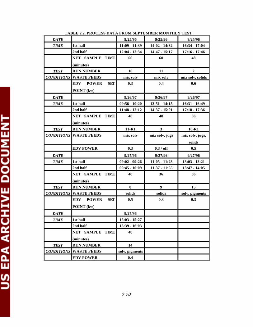
2-522-52

TABLE 2.2. PROCESS DATA FROM SEPTEMBER MONTHLY TEST

DATE 9/25/96 9/25/96 9/25/96

TIME 1st half 11:09 - 11:39 14:02 - 14:32 16:34 - 17:04

2nd half 12:04 - 12:34 14:47 - 15:17 17:16 - 17:46NET SAMPLE TIME 60 60 48

(minutes)TEST RUN NUMBER 10 11 2

CONDITIONS WASTE FEEDS mix solv mix solv mix solv, solidsEDV POWER SET 0.3 0.4 0.6

POINT (kw)

DATE 9/26/97 9/26/97 9/26/97

TIME 1st half 09:56 - 10:20 13:51 - 14:15 16:31 - 16:492nd half 11:48 - 12:12 14:37 - 15:01 17:18 - 17:36

NET SAMPLE TIME 48 48 36

(minutes)

TEST RUN NUMBER 11-R1 3 10-R1

CONDITIONS WASTE FEEDS mix solv mix solv, jugs mix solv, jugs,

solidsEDV POWER 0.3 0.3 / off 0.5

DATE 9/27/96 9/27/96 9/27/96

TIME 1st half 09:02 - 09:26 11:05 - 11:23 13:03 - 13:21

2nd half 09:45 - 10:09 11:37 - 11:55 13:47 - 14:05NET SAMPLE TIME 48 36 36

(minutes)TEST RUN NUMBER 8 9 15

CONDITIONS WASTE FEEDS solids solids solv, pigmentsEDV POWER SET 0.5 0.3 0.3

POINT (kw)

DATE 9/27/96

TIME 1st half 15:03 - 15:272nd half 15:39 - 16:03

NET SAMPLE TIME 48

(minutes)

TEST RUN NUMBER 14

CONDITIONS WASTE FEEDS solv, pigments

EDV POWER 0.4

2-532-53

TABLE 2.2 (CONT.). PROCESS DATA FROM OCTOBER MONTHLY TEST

DATE 10/15/96 10/15/96 10/16/96

TIME 1st half 14:02 - 14:20 16:10 - 16:28 12:44 - 12:56

2nd half 14:32 - 14:50 16:41 - 16:59 13:04 - 13:16NET SAMPLE TIME 36 36 24

(minutes)TEST RUN NUMBER 4 5 6

CONDITIONS WASTE FEEDS pigments solvents solventsEDV POWER SET 1 0.6 0.3

POINT (kw)

DATE 10/17/96 10/17/96 10/17/96

TIME 1st half 08:37 - 08:49 10:15 - 10:24 11:57 - 12:062nd half 09:01 - 09:13 10:38 - 10:47 12:19 - 12:28

NET SAMPLE TIME 24 18 18

(minutes)

TEST RUN NUMBER 6-R1 6-R2 16

CONDITIONS WASTE FEEDS solvents, oil, solvents, oil, solids oil, solids

solidsEDV POWER 0.3 0.3 0.8

DATE 10/17/96 10/17/96 10/17/96

TIME 1st half 14:15 - 14:24 15:10 - 15:19 17:06 - 17:15

2nd half 14:31 - 14:40 16:18 - 16:27 17:23 - 17:32NET SAMPLE TIME 18 18 18

(minutes)TEST RUN NUMBER 17 18 19

CONDITIONS WASTE FEEDS oil, solids oil, solids solvents, solidsEDV POWER SET 0.7 0.7 1.1

POINT (kw)

DATE 10/18/96 10/18/96

TIME 1st half 10:15 - 10:33 13:16 - 13:402nd half 10:47 - 11:05 13:54 - 14:18

NET SAMPLE TIME 36 48

(minutes)

TEST RUN NUMBER 20 21

CONDITIONS WASTE FEEDS oil oil

EDV POWER 0.7 0.7

2-542-54

TABLE 2.2 (CONT.). PROCESS DATA FROM NOVEMBER MONTHLY TEST

DATE 11/12/96 11/12/96 11/12/96

TIME 1st half 12:44 - 13:02 14:12 - 14:30 15:59 - 16:17

2nd half 13:12 - 13:30 14:37 - 14:55 16:26 - 16:44NET SAMPLE TIME 36 36 36

(minutes)TEST RUN NUMBER 22 23 24

CONDITIONS WASTE FEEDS oil oil, jugs, solids oil, jugs, solidsEDV POWER SET 1.1 1.1 1.1

POINT (kw)

DATE 11/13/96 11/13/96 11/13/96

TIME 1st half 08:44 - 09:08 10:24 - 10:48 12:09 - 12:332nd half 09:15 - 09:39 10:55 - 11:19 12:42 - 13:06

NET SAMPLE TIME 48 48 48

(minutes)

TEST RUN NUMBER 25 26 27

CONDITIONS WASTE FEEDS solvents, jugs, solvents, jugs, oil, jugs, solids

solids solidsEDV POWER SET 0.7 0.7 0.7

POINT (kw)

DATE 11/13/96 11/13/96 11/14/96

TIME 1st half 15:11 - 15:29 16:38 - 16:56 15:42 - 16:002nd half 15:37 - 15:55 17:04 - 17:22 16:09 - 16:27

NET SAMPLE TIME 36 36 36

(minutes)

TEST RUN NUMBER 28 29 30

CONDITIONS WASTE FEEDS solvents, jugs, oil oil, jugs, solids

solidsEDV POWER SET 0.3 0.3 0.3

POINT (kw)

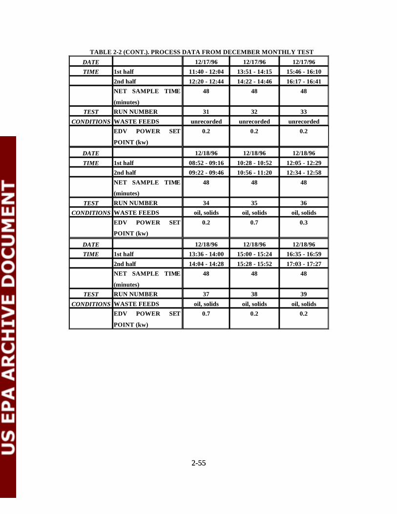
2-552-55

TABLE 2-2 (CONT.). PROCESS DATA FROM DECEMBER MONTHLY TEST

DATE 12/17/96 12/17/96 12/17/96

TIME 1st half 11:40 - 12:04 13:51 - 14:15 15:46 - 16:10

2nd half 12:20 - 12:44 14:22 - 14:46 16:17 - 16:41NET SAMPLE TIME 48 48 48

(minutes)TEST RUN NUMBER 31 32 33

CONDITIONS WASTE FEEDS unrecorded unrecorded unrecordedEDV POWER SET 0.2 0.2 0.2

POINT (kw)

DATE 12/18/96 12/18/96 12/18/96

TIME 1st half 08:52 - 09:16 10:28 - 10:52 12:05 - 12:292nd half 09:22 - 09:46 10:56 - 11:20 12:34 - 12:58

NET SAMPLE TIME 48 48 48

(minutes)

TEST RUN NUMBER 34 35 36

CONDITIONS WASTE FEEDS oil, solids oil, solids oil, solids

EDV POWER SET 0.2 0.7 0.3

POINT (kw)

DATE 12/18/96 12/18/96 12/18/96

TIME 1st half 13:36 - 14:00 15:00 - 15:24 16:35 - 16:59

2nd half 14:04 - 14:28 15:28 - 15:52 17:03 - 17:27NET SAMPLE TIME 48 48 48

(minutes)TEST RUN NUMBER 37 38 39

CONDITIONS WASTE FEEDS oil, solids oil, solids oil, solidsEDV POWER SET 0.7 0.2 0.2

POINT (kw)

2-562-56

TABLE 2-2 (CONT.). PROCESS DATA FROM JANUARY MONTHLY TEST

DATE 1/15/97 1/15/97 1/15/97

TIME 1st half 09:25 - 09:49 11:47 - 12:11 14:57 - 15:21

2nd half 10:14 - 10:38 12:57 - 13:21 15:28 - 15:52NET SAMPLE TIME 48 48 48(minutes)

TEST RUN NUMBER 40 41 42

CONDITIONS WASTE FEEDS oil, jugs oil, jugs, solids oil, solids

EDV POWER SET 1.5 1.0 1.0POINT (kw)

DATE 1/16/97 1/16/97 1/16/97

TIME 1st half 12:25 - 12:49 13:40 - 14:04 15:00 - 15:242nd half 12:55 - 13:19 14:10 - 14:34 15:40 - 16:04

NET SAMPLE TIME 48 48 48(minutes)

TEST RUN NUMBER 43 44 45

CONDITIONS WASTE FEEDS chlor solv, solids chlor solv, jugs, chlor solv, solidssolids

EDV POWER SET 1.0 1.0 1.0POINT (kw)

DATE 1/16/97 1/17/97 1/17/97

TIME 1st half 16:38 - 17:02 08:39- 12:22 - 12:4608:43/09:50-

10:102nd half 17:08 - 17:32 10:19 - 10:43 12:53 - 13:17NET SAMPLE TIME 48 48 48(minutes)

TEST RUN NUMBER 46 47 48

CONDITIONS WASTE FEEDS chlor solv, oil, chlor solv, jugs, chlor solv, jugs,jugs solids solids

EDV POWER SET 1.0 1.0 1.0POINT (kw)

DATE 1/17/97

TIME 1st half 14:57 - 15:212nd half 15:46 - 16:10

NET SAMPLE TIME 48(minutes)

TEST RUN NUMBER 49

CONDITIONS WASTE FEEDS chlor solvents, jugs, solids

EDV POWER SET 1.0POINT (kw)

2-572-57

TABLE 2-2 (CONT.). PROCESS DATA FROM FEBRUARY MONTHLY TEST

DATE 2/19/97 2/19/97 2/19/97

TIME 1st half 9:45 - 10:15 11:59 -12:35 14:29 - 15:05

2nd half 10:24 - 10:54 12:45 - 13:21 15:13 - 15:49NET SAMPLE TIME 60 72 72(minutes)

TEST RUN NUMBER 50 51 52

CONDITIONS WASTE FEEDS oil, solids oil, jugs, solids oil, jugs, solids

EDV POWER SET 2.0 2.0 1.0POINT (kw)

DATE 2/19/97 2/20/97 2/20/97

TIME 1st half 16:28 -17:04 8:30 - 9:06 10:50 - 11:262nd half 17:13 - 17:49 9:13 - 9:49 11:34 - 12:10

NET SAMPLE TIME 72 72 72(minutes)

TEST RUN NUMBER 53 54 55

CONDITIONS WASTE FEEDS oil, solids mixed solv, jugs, mixed solv,solids, pigment jugs, solids

EDV POWER SET 1.0 1.0 1.0POINT (kw)

DATE 2/20/97 2/20/97 2/21/97

TIME 1st half 12:59 - 13:35 15:19 - 15:55 8:33 - 9:09

2nd half 13:46 - 14:22 16:02 - 16:38 9:15 - 9:51NET SAMPLE TIME 72 72 72(minutes)

TEST RUN NUMBER 56 57 58

CONDITIONS WASTE FEEDS mixed solv, jugs mixed solv, mixed solv,jugs,solids jugs,solids

EDV POWER SET 1.0 1.0 1.0POINT (kw)

DATE 2/21/97 2/21/97 2/21/97

TIME 1st half 10:41 - 11:17 12:33 - 13:09 14:49 - 15:252nd half 11:23 - 11:59 13:45 - 14:21 15:31 - 16:07

NET SAMPLE TIME 72 72 72(minutes)

TEST RUN NUMBER 59 60 61

CONDITIONS WASTE FEEDS mixed solv, mixed solv, jugs mixed solv,jugs,solids solids

EDV POWER SET 1.0 1.0 1.0POINT (kw)

2-582-58

TABLE 2-2 (CONT.). PROCESS DATA FROM MARCH MONTHLY TEST

DATE 3/18/97 3/18/97 3/18/97

TIME 1st half 10:55 - 11:25 13:00 - 13:30 14:56 - 15:26

2nd half 11:32 - 12:02 13:38 - 14:08 15:32 - 16:02NET SAMPLE TIME 60 60 60(minutes)

TEST RUN NUMBER 62 63 64

CONDITIONS WASTE FEEDS oil, jugs, solids oil, jugs oil, jugs,solids

EDV POWER SET 2.0 2.0 2.0POINT (kw)

DATE 3/19/97 3/19/97 3/19/97

TIME 1st half 8:43 - 9:13 10:36 - 11:06 14:30 - 15:002nd half 9:20 - 9:50 11:24 - 11:54 15:06 - 15:36

NET SAMPLE TIME 60 60 60(minutes)

TEST RUN NUMBER 65 66 67

CONDITIONS WASTE FEEDS oil, mixed solv, jugs, mixed solv, jugsjugs,solids,pigme solids, pigment

ntEDV POWER SET 2.0 1.0 1.0POINT (kw)

DATE 3/19/97 3/20/97 3/20/97

TIME 1st half 16:56 - 17:26 9:08 - 9:38 10:49 - 11:19

2nd half 17:30 - 18:00 9:44 - 10:14 11:29 - 11:59NET SAMPLE TIME 60 60 60(minutes)

TEST RUN NUMBER 68 69 70

CONDITIONS WASTE FEEDS mixed solv, oil, mixed solv, jugs mixed solv,solids jugs, solids,

pigmentEDV POWER SET 1.0 1.0 1.0POINT (kw)

DATE 3/20/97 3/20/97 3/20/97

TIME 1st half 12:51 - 13:21 14:42 - 15:12 16:33 - 17:032nd half 13:27 - 13:57 15:18 - 15:48 17:35 - 18:05

NET SAMPLE TIME 60 60 60(minutes)

TEST RUN NUMBER 71 72 73

CONDITIONS WASTE FEEDS mixed solv, solids mixed solv, mixed solv,jugs,solids solids

EDV POWER SET 1.0 1.0 1.0POINT (kw)

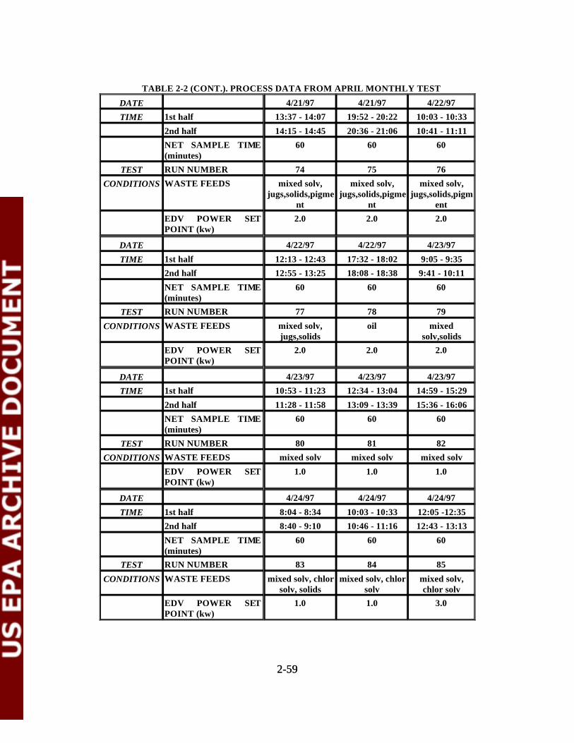
2-592-59

TABLE 2-2 (CONT.). PROCESS DATA FROM APRIL MONTHLY TEST

DATE 4/21/97 4/21/97 4/22/97

TIME 1st half 13:37 - 14:07 19:52 - 20:22 10:03 - 10:33

2nd half 14:15 - 14:45 20:36 - 21:06 10:41 - 11:11NET SAMPLE TIME 60 60 60(minutes)

TEST RUN NUMBER 74 75 76

CONDITIONS WASTE FEEDS mixed solv, mixed solv, mixed solv,jugs,solids,pigme jugs,solids,pigme jugs,solids,pigm

nt nt entEDV POWER SET 2.0 2.0 2.0POINT (kw)

DATE 4/22/97 4/22/97 4/23/97

TIME 1st half 12:13 - 12:43 17:32 - 18:02 9:05 - 9:352nd half 12:55 - 13:25 18:08 - 18:38 9:41 - 10:11

NET SAMPLE TIME 60 60 60(minutes)

TEST RUN NUMBER 77 78 79

CONDITIONS WASTE FEEDS mixed solv, oil mixedjugs,solids solv,solids

EDV POWER SET 2.0 2.0 2.0POINT (kw)

DATE 4/23/97 4/23/97 4/23/97

TIME 1st half 10:53 - 11:23 12:34 - 13:04 14:59 - 15:29

2nd half 11:28 - 11:58 13:09 - 13:39 15:36 - 16:06NET SAMPLE TIME 60 60 60(minutes)

TEST RUN NUMBER 80 81 82

CONDITIONS WASTE FEEDS mixed solv mixed solv mixed solv

EDV POWER SET 1.0 1.0 1.0POINT (kw)

DATE 4/24/97 4/24/97 4/24/97

TIME 1st half 8:04 - 8:34 10:03 - 10:33 12:05 -12:352nd half 8:40 - 9:10 10:46 - 11:16 12:43 - 13:13

NET SAMPLE TIME 60 60 60(minutes)

TEST RUN NUMBER 83 84 85

CONDITIONS WASTE FEEDS mixed solv, chlor mixed solv, chlor mixed solv,solv, solids solv chlor solv

EDV POWER SET 1.0 1.0 3.0POINT (kw)

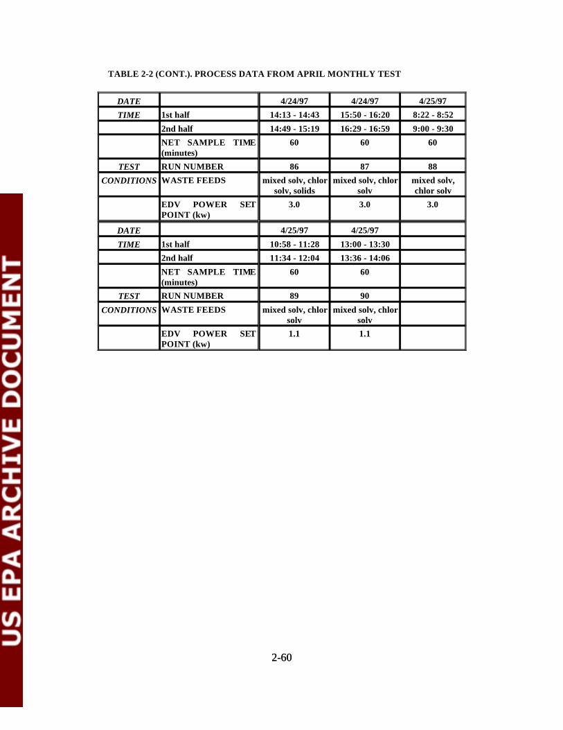
2-602-60

TABLE 2-2 (CONT.). PROCESS DATA FROM APRIL MONTHLY TEST

DATE 4/24/97 4/24/97 4/25/97

TIME 1st half 14:13 - 14:43 15:50 - 16:20 8:22 - 8:52

2nd half 14:49 - 15:19 16:29 - 16:59 9:00 - 9:30NET SAMPLE TIME 60 60 60(minutes)

TEST RUN NUMBER 86 87 88

CONDITIONS WASTE FEEDS mixed solv, chlor mixed solv, chlor mixed solv,solv, solids solv chlor solv

EDV POWER SET 3.0 3.0 3.0POINT (kw)

DATE 4/25/97 4/25/97

TIME 1st half 10:58 - 11:28 13:00 - 13:302nd half 11:34 - 12:04 13:36 - 14:06

NET SAMPLE TIME 60 60(minutes)

TEST RUN NUMBER 89 90

CONDITIONS WASTE FEEDS mixed solv, chlor mixed solv, chlorsolv solv

EDV POWER SET 1.1 1.1POINT (kw)

2-612-61

TABLE 2-2 (CONT.). PROCESS DATA FROM MAY MONTHLY TEST

DATE 5/20/97 5/20/97 5/20/97

TIME 1st half 10:12 - 10:42 13:50 - 14:20 16:36 - 17:06

2nd half 10:49 - 11:31 14:25 - 14:55 17:15 - 17:45NET SAMPLE TIME 60 60 60(minutes)

TEST RUN NUMBER 91 92 93

CONDITIONS WASTE FEEDS mixed solv, solids mixed solv, solids mixed solv

EDV POWER SET 3.0 3.0 3.0POINT (kw)

DATE 5/21/97 5/21/97 5/22/97

TIME 1st half 13:51 - 14:21 16:07 - 16:37 9:35 - 10:202nd half 14:29 - 14:59 16:45 - 17:15 10:33 - 11:18

NET SAMPLE TIME 60 60 90(minutes)

TEST RUN NUMBER 94 95 96

CONDITIONS WASTE FEEDS mixed solv, solids mixed solv, oilsolids, pigments,

jugsEDV POWER SET 1.5 1.5 1.5POINT (kw)

DATE 5/22/97 5/22/97 5/23/97

TIME 1st half 14:04 - 14:34 16:07 - 16:37 7:53 - 8:23

2nd half 14:42 - 15:12 16:44 - 17:22 8:30 - 9:00NET SAMPLE TIME 60 60 60(minutes)

TEST RUN NUMBER 97 98 99

CONDITIONS WASTE FEEDS mixed solv, mixed solv, solids mixed solv,solids, pigments, solids, jugs

jugsEDV POWER SET 1.5 1.5 1.5POINT (kw)

DATE 5/23/97 5/23/97 5/23/97

TIME 1st half 9:43 - 10:13 12:03 - 12:33 13:59 - 14:292nd half 10:22 - 10:52 12:45 - 13:15 14:47 - 15:17

NET SAMPLE TIME 60 60 60(minutes)

TEST RUN NUMBER 100 101 102

CONDITIONS WASTE FEEDS mixed solv, mixed solv, mixed solv,solids, pigments, solids, pigments, solids, jugs

jugs jugsEDV POWER SET 1.5 1.0 1.0POINT (kw)

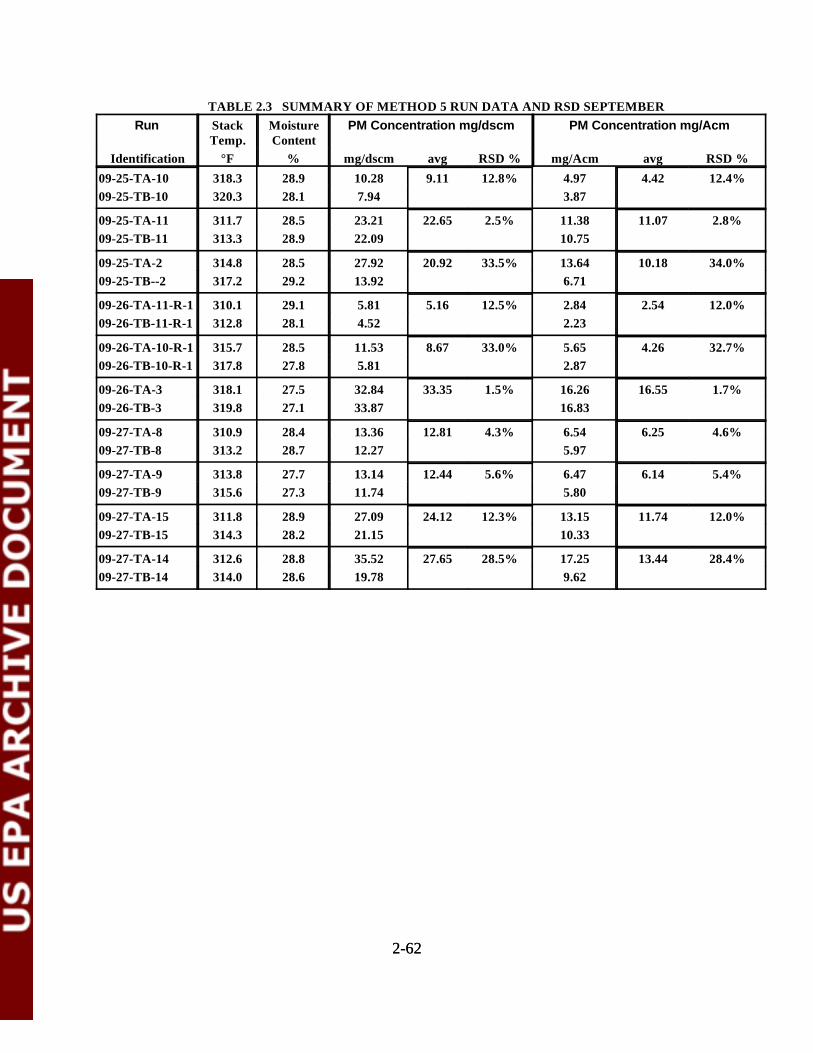
2-622-62

TABLE 2.3 SUMMARY OF METHOD 5 RUN DATA AND RSD SEPTEMBERRun Stack Moisture PM Concentration mg/dscm PM Concentration mg/Acm

Temp. ContentIdentification °F % mg/dscm avg RSD % mg/Acm avg RSD %

09-25-TA-10 318.3 28.9 10.28 9.11 12.8% 4.97 4.42 12.4%09-25-TB-10 320.3 28.1 7.94 3.87

09-25-TA-11 311.7 28.5 23.21 22.65 2.5% 11.38 11.07 2.8%09-25-TB-11 313.3 28.9 22.09 10.75

09-25-TA-2 314.8 28.5 27.92 20.92 33.5% 13.64 10.18 34.0%09-25-TB--2 317.2 29.2 13.92 6.71

09-26-TA-11-R-1 310.1 29.1 5.81 5.16 12.5% 2.84 2.54 12.0%09-26-TB-11-R-1 312.8 28.1 4.52 2.23

09-26-TA-10-R-1 315.7 28.5 11.53 8.67 33.0% 5.65 4.26 32.7%09-26-TB-10-R-1 317.8 27.8 5.81 2.87

09-26-TA-3 318.1 27.5 32.84 33.35 1.5% 16.26 16.55 1.7%09-26-TB-3 319.8 27.1 33.87 16.83

09-27-TA-8 310.9 28.4 13.36 12.81 4.3% 6.54 6.25 4.6%09-27-TB-8 313.2 28.7 12.27 5.97

09-27-TA-9 313.8 27.7 13.14 12.44 5.6% 6.47 6.14 5.4%09-27-TB-9 315.6 27.3 11.74 5.80

09-27-TA-15 311.8 28.9 27.09 24.12 12.3% 13.15 11.74 12.0%09-27-TB-15 314.3 28.2 21.15 10.33

09-27-TA-14 312.6 28.8 35.52 27.65 28.5% 17.25 13.44 28.4%09-27-TB-14 314.0 28.6 19.78 9.62

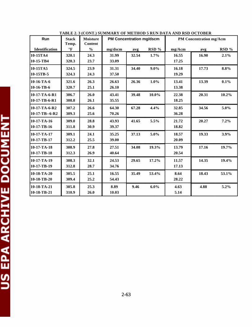
2-632-63

TABLE 2. 3 (CONT.) SUMMARY OF METHOD 5 RUN DATA AND RSD OCTOBERRun Stack Moisture PM Concentration mg/dscm PM Concentration mg/Acm

Temp. ContentIdentification °F % mg/dscm avg RSD % mg/Acm avg RSD %

10-15TA4 320.1 24.3 31.99 32.54 1.7% 16.55 16.90 2.1%10-15-TB4 320.3 23.7 33.09 17.25

10-15TA5 324.5 23.9 31.31 34.40 9.0% 16.18 17.73 8.8%10-15TB-5 324.3 24.3 37.50 19.29

10-16-TA-6 321.6 26.3 26.63 26.36 1.0% 13.41 13.39 0.1%10-16-TB-6 320.7 25.1 26.10 13.38

10-17-TA-6-R1 306.7 26.0 43.41 39.48 10.0% 22.38 20.31 10.2%10-17-TB-6-R1 308.8 26.1 35.55 18.25

10-17-TA-6-R2 307.2 26.6 64.30 67.28 4.4% 32.85 34.56 5.0%10-17-TB--6-R2 309.3 25.6 70.26 36.28

10-17-TA-16 309.0 28.8 43.93 41.65 5.5% 21.72 20.27 7.2%10-17-TB-16 311.8 30.9 39.37 18.82

10-17-TA-17 309.1 24.1 35.25 37.13 5.0% 18.57 19.33 3.9%10-17-TB-17 312.2 25.5 39.00 20.09

10-17-TA-18 308.9 27.8 27.51 34.08 19.3% 13.79 17.16 19.7%10-17-TB-18 312.3 26.9 40.64 20.54

10-17-TA-19 308.3 32.1 24.53 29.65 17.2% 11.57 14.35 19.4%10-17-TB-19 312.8 28.7 34.76 17.13

10-18-TA-20 305.5 25.1 16.55 35.49 53.4% 8.64 18.43 53.1%10-18-TB-20 309.4 25.2 54.43 28.22

10-18-TA-21 305.8 25.3 8.89 9.46 6.0% 4.63 4.88 5.2%10-18-TB-21 310.9 26.0 10.03 5.14

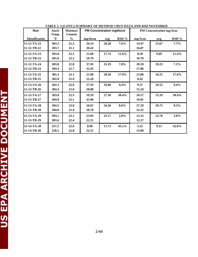
2-642-64

TABLE 2. 3 (CONT.) SUMMARY OF METHOD 5 RUN DATA AND RSD NOVEMBERRun Stack Moisture PM Concentration mg/dscm PM Concentration mg/Acm

Temp. ContentIdentification °F % mg/dscm avg RSD % mg/Acm avg RSD %

11-12-TA-22 303.3 21.3 26.14 28.28 7.6% 14.47 15.67 7.7%11-12-TB-22 303.7 21.1 30.42 16.87

11-12-TA-23 303.8 22.1 15.68 17.74 11.6% 8.59 9.69 11.4%11-12-TB-23 305.9 22.3 19.79 10.79

11-12-TA-24 303.8 22.8 37.92 35.19 7.8% 20.59 19.23 7.1%11-12-TB-24 304.4 21.7 32.45 17.86

11-13-TA-25 305.3 22.1 21.80 18.50 17.9% 12.00 10.21 17.6%11-13-TB-25 302.8 21.9 15.20 8.42

11-13-TA-26 302.3 22.0 17.29 19.08 9.4% 9.57 10.55 9.4%11-13-TB-26 304.4 21.8 20.88 11.54

11-13-TA-27 303.0 22.3 19.19 27.58 30.4% 10.57 15.19 30.4%11-13-TB-27 304.9 22.1 35.96 19.81

11-13-TA-28 304.5 22.8 50.01 54.36 8.0% 27.29 29.75 8.3%11-13-TB-28 304.8 22.4 58.70 32.22

11-13-TA-29 303.1 22.1 23.83 23.17 2.8% 13.15 12.76 3.0%11-13-TB-29 303.6 22.4 22.51 12.37

11-14-TA-30 257.5 22.6 8.96 15.73 43.1% 5.22 9.15 42.9%11-14-TB-30 258.5 22.8 22.51 13.08

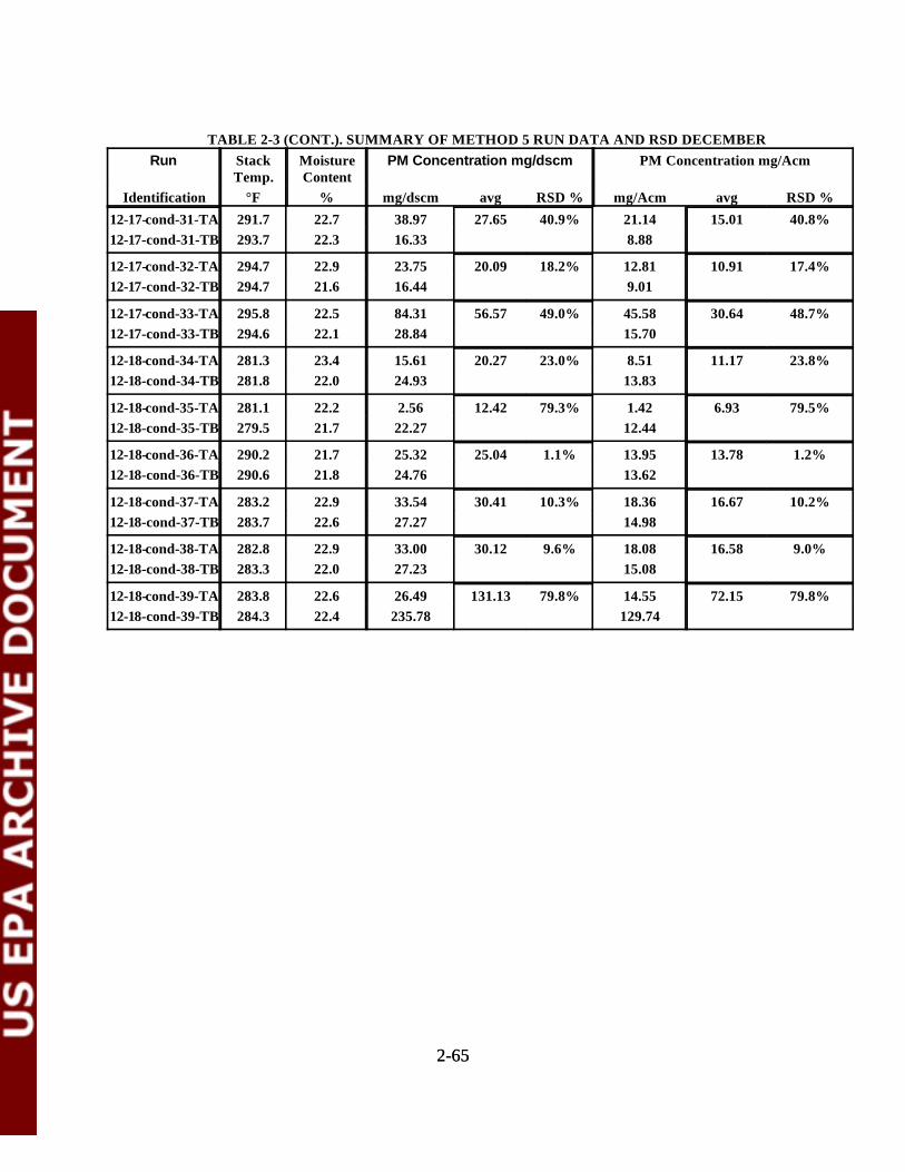
2-652-65

TABLE 2-3 (CONT.). SUMMARY OF METHOD 5 RUN DATA AND RSD DECEMBERRun Stack Moisture PM Concentration mg/dscm PM Concentration mg/Acm

Temp. ContentIdentification °F % mg/dscm avg RSD % mg/Acm avg RSD %

12-17-cond-31-TA 291.7 22.7 38.97 27.65 40.9% 21.14 15.01 40.8%12-17-cond-31-TB 293.7 22.3 16.33 8.88

12-17-cond-32-TA 294.7 22.9 23.75 20.09 18.2% 12.81 10.91 17.4%12-17-cond-32-TB 294.7 21.6 16.44 9.01

12-17-cond-33-TA 295.8 22.5 84.31 56.57 49.0% 45.58 30.64 48.7%12-17-cond-33-TB 294.6 22.1 28.84 15.70

12-18-cond-34-TA 281.3 23.4 15.61 20.27 23.0% 8.51 11.17 23.8%12-18-cond-34-TB 281.8 22.0 24.93 13.83

12-18-cond-35-TA 281.1 22.2 2.56 12.42 79.3% 1.42 6.93 79.5%12-18-cond-35-TB 279.5 21.7 22.27 12.44

12-18-cond-36-TA 290.2 21.7 25.32 25.04 1.1% 13.95 13.78 1.2%12-18-cond-36-TB 290.6 21.8 24.76 13.62

12-18-cond-37-TA 283.2 22.9 33.54 30.41 10.3% 18.36 16.67 10.2%12-18-cond-37-TB 283.7 22.6 27.27 14.98

12-18-cond-38-TA 282.8 22.9 33.00 30.12 9.6% 18.08 16.58 9.0%12-18-cond-38-TB 283.3 22.0 27.23 15.08

12-18-cond-39-TA 283.8 22.6 26.49 131.13 79.8% 14.55 72.15 79.8%12-18-cond-39-TB 284.3 22.4 235.78 129.74

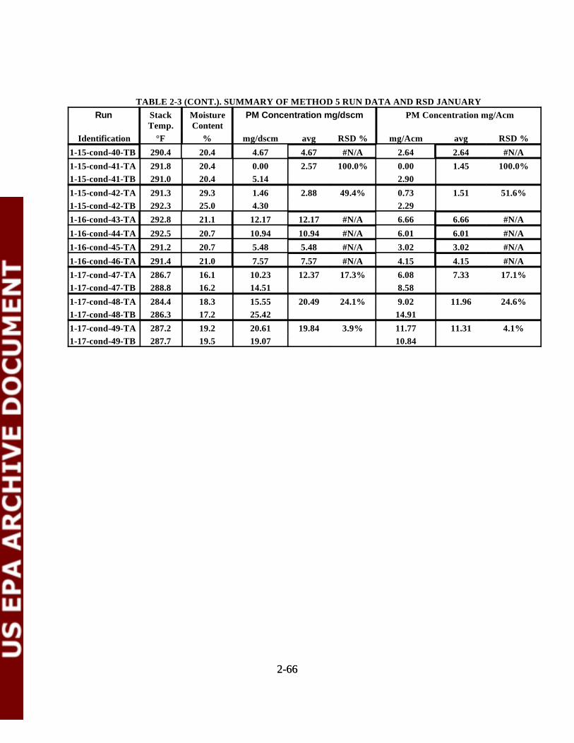
2-662-66

TABLE 2-3 (CONT.). SUMMARY OF METHOD 5 RUN DATA AND RSD JANUARYRun Stack Moisture PM Concentration mg/dscm PM Concentration mg/Acm

Temp. ContentIdentification °F % mg/dscm avg RSD % mg/Acm avg RSD %

1-15-cond-40-TB 290.4 20.4 4.67 4.67 #N/A 2.64 2.64 #N/A1-15-cond-41-TA 291.8 20.4 0.00 2.57 100.0% 0.00 1.45 100.0%1-15-cond-41-TB 291.0 20.4 5.14 2.901-15-cond-42-TA 291.3 29.3 1.46 2.88 49.4% 0.73 1.51 51.6%1-15-cond-42-TB 292.3 25.0 4.30 2.291-16-cond-43-TA 292.8 21.1 12.17 12.17 #N/A 6.66 6.66 #N/A1-16-cond-44-TA 292.5 20.7 10.94 10.94 #N/A 6.01 6.01 #N/A1-16-cond-45-TA 291.2 20.7 5.48 5.48 #N/A 3.02 3.02 #N/A1-16-cond-46-TA 291.4 21.0 7.57 7.57 #N/A 4.15 4.15 #N/A1-17-cond-47-TA 286.7 16.1 10.23 12.37 17.3% 6.08 7.33 17.1%1-17-cond-47-TB 288.8 16.2 14.51 8.581-17-cond-48-TA 284.4 18.3 15.55 20.49 24.1% 9.02 11.96 24.6%1-17-cond-48-TB 286.3 17.2 25.42 14.911-17-cond-49-TA 287.2 19.2 20.61 19.84 3.9% 11.77 11.31 4.1%1-17-cond-49-TB 287.7 19.5 19.07 10.84

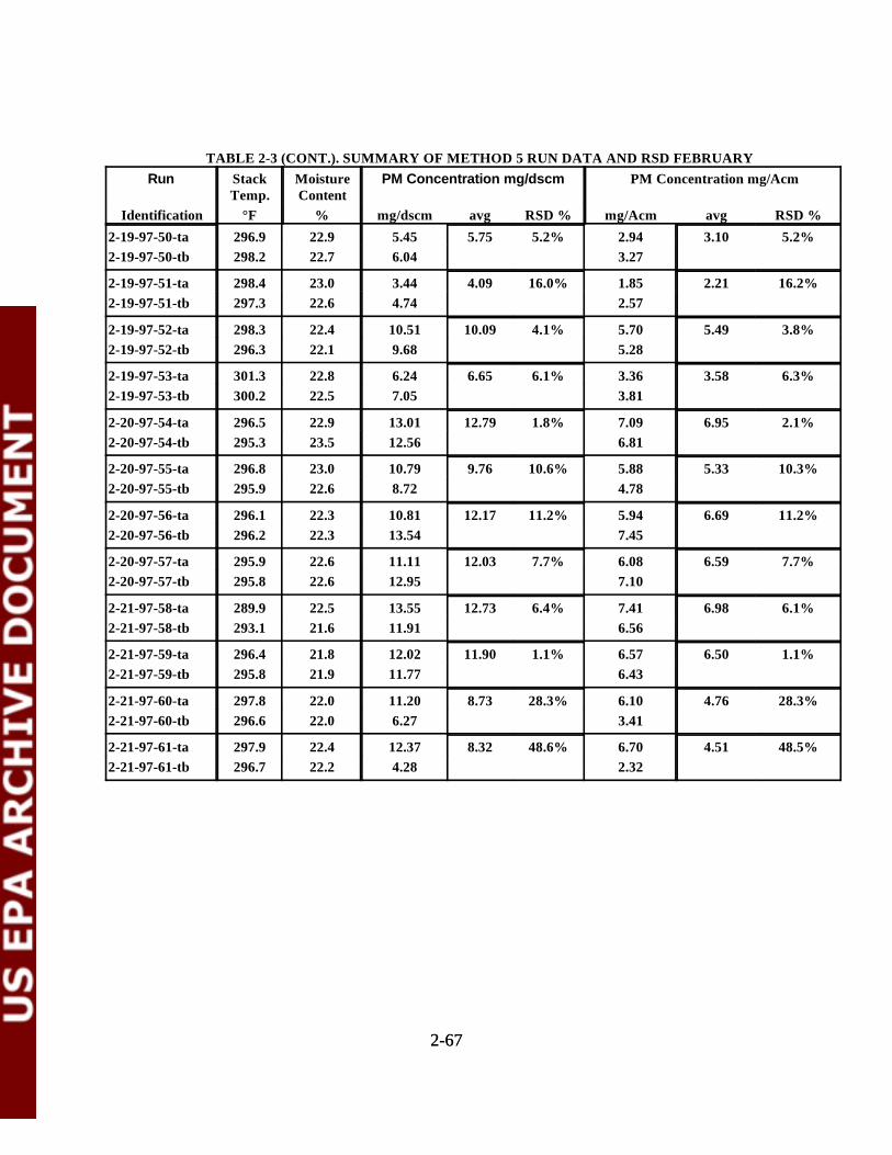
2-672-67

TABLE 2-3 (CONT.). SUMMARY OF METHOD 5 RUN DATA AND RSD FEBRUARYRun Stack Moisture PM Concentration mg/dscm PM Concentration mg/Acm

Temp. ContentIdentification °F % mg/dscm avg RSD % mg/Acm avg RSD %

2-19-97-50-ta 296.9 22.9 5.45 5.75 5.2% 2.94 3.10 5.2%2-19-97-50-tb 298.2 22.7 6.04 3.27

2-19-97-51-ta 298.4 23.0 3.44 4.09 16.0% 1.85 2.21 16.2%2-19-97-51-tb 297.3 22.6 4.74 2.57

2-19-97-52-ta 298.3 22.4 10.51 10.09 4.1% 5.70 5.49 3.8%2-19-97-52-tb 296.3 22.1 9.68 5.28

2-19-97-53-ta 301.3 22.8 6.24 6.65 6.1% 3.36 3.58 6.3%2-19-97-53-tb 300.2 22.5 7.05 3.81

2-20-97-54-ta 296.5 22.9 13.01 12.79 1.8% 7.09 6.95 2.1%2-20-97-54-tb 295.3 23.5 12.56 6.81

2-20-97-55-ta 296.8 23.0 10.79 9.76 10.6% 5.88 5.33 10.3%2-20-97-55-tb 295.9 22.6 8.72 4.78

2-20-97-56-ta 296.1 22.3 10.81 12.17 11.2% 5.94 6.69 11.2%2-20-97-56-tb 296.2 22.3 13.54 7.45

2-20-97-57-ta 295.9 22.6 11.11 12.03 7.7% 6.08 6.59 7.7%2-20-97-57-tb 295.8 22.6 12.95 7.10

2-21-97-58-ta 289.9 22.5 13.55 12.73 6.4% 7.41 6.98 6.1%2-21-97-58-tb 293.1 21.6 11.91 6.56

2-21-97-59-ta 296.4 21.8 12.02 11.90 1.1% 6.57 6.50 1.1%2-21-97-59-tb 295.8 21.9 11.77 6.43

2-21-97-60-ta 297.8 22.0 11.20 8.73 28.3% 6.10 4.76 28.3%2-21-97-60-tb 296.6 22.0 6.27 3.41

2-21-97-61-ta 297.9 22.4 12.37 8.32 48.6% 6.70 4.51 48.5%2-21-97-61-tb 296.7 22.2 4.28 2.32

2-682-68

TABLE 2-3 (CONT.). SUMMARY OF METHOD 5 RUN DATA AND RSD MARCHRun Stack Moisture PM Concentration mg/dscm PM Concentration mg/Acm

Temp. ContentIdentification °F % mg/dscm avg RSD % mg/Acm avg RSD %

3-18-97-62-ta 291.8 16.8 16.18 16.50 1.9% 9.56 9.78 2.2%3-18-97-62-tb 293.9 16.0 16.81 10.00

3-18-97-63-ta 292.8 17.0 16.47 17.32 4.9% 9.70 10.22 5.1%3-18-97-63-tb 294.1 16.5 18.18 10.74

3-18-97-64-ta 291.8 17.5 19.85 18.43 7.7% 11.63 10.83 7.3%3-18-97-64-tb 292.9 16.8 17.01 10.04

3-19-97-65-ta 289.3 17.3 33.59 31.98 5.0% 19.74 18.82 4.9%3-19-97-65-tb 291.1 16.9 30.37 17.89

3-19-97-66-ta 291.9 17.3 51.05 49.09 4.0% 29.91 29.03 3.0%3-19-97-66-tb 291.3 15.7 47.12 28.14

3-19-97-67-ta 291.8 17.0 50.32 49.07 2.5% 29.57 28.89 2.4%3-19-97-67-tb 293.4 16.5 47.82 28.21

3-19-97-68-ta 293.9 16.3 14.83 15.22 2.6% 8.77 8.98 2.4%3-19-97-68-tb 296.1 16.3 15.61 9.20

3-20-97-69-ta 279.5 15.0 38.37 37.18 3.2% 23.25 22.36 4.0%3-20-97-69-tb 291.7 14.9 35.99 21.48

3-20-97-70-ta 291.6 13.6 28.13 26.27 7.1% 17.05 15.94 6.9%3-20-97-70-tb 291.9 13.3 24.42 14.84

3-20-97-71-ta 291.3 13.7 #N/A 33.26 0.0% #N/A 20.18 0.0%3-20-97-71-tb 292.0 13.4 33.26 20.18

3-20-97-72-ta 293.7 13.9 23.81 22.82 4.3% 14.34 13.76 4.2%3-20-97-72-tb 293.5 13.6 21.83 13.19

3-20-97-73-ta 290.8 13.6 5.99 6.33 5.2% 3.64 3.84 5.3%3-20-97-73-tb 291.7 13.4 6.66 4.04

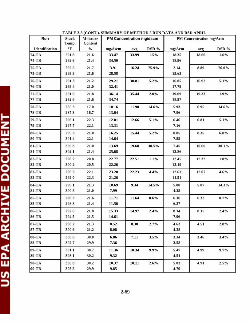
2-692-69

TABLE 2-3 (CONT.). SUMMARY OF METHOD 5 RUN DATA AND RSD APRILRun Stack Moisture PM Concentration mg/dscm PM Concentration mg/Acm

Temp. ContentIdentification °F % mg/dscm avg RSD % mg/Acm avg RSD %

74-TA 291.8 21.6 33.47 33.99 1.5% 18.35 18.66 1.6%74-TB 292.6 21.4 34.50 18.96

75-TA 292.5 21.7 3.91 16.24 75.9% 2.14 8.89 76.0%75-TB 293.3 21.6 28.58 15.65

76-TA 291.3 21.2 29.21 30.81 5.2% 16.05 16.92 5.1%76-TB 293.4 21.0 32.41 17.79

77-TA 291.9 21.8 36.14 35.44 2.0% 19.69 19.33 1.9%77-TB 292.6 21.6 34.74 18.97

78-TA 285.3 17.0 10.16 11.90 14.6% 5.93 6.95 14.6%78-TB 287.3 16.7 13.64 7.96

79-TA 296.1 22.3 12.01 12.66 5.1% 6.46 6.81 5.1%79-TB 297.7 22.1 13.31 7.16

80-TA 299.3 21.0 16.25 15.44 5.2% 8.85 8.35 6.0%80-TB 301.4 22.1 14.64 7.85

81-TA 300.8 21.0 13.69 19.68 30.5% 7.45 10.66 30.1%81-TB 302.1 21.4 25.68 13.86

82-TA 298.2 20.8 22.77 22.51 1.1% 12.45 12.32 1.0%82-TB 300.2 20.5 22.26 12.19

83-TA 289.3 22.1 23.20 22.23 4.4% 12.63 12.07 4.6%83-TB 292.0 22.3 21.26 11.51

84-TA 299.1 21.3 10.69 9.34 14.5% 5.80 5.07 14.3%84-TB 300.8 21.0 7.99 4.35

85-TA 296.3 21.6 11.71 11.64 0.6% 6.36 6.32 0.7%85-TB 298.8 21.4 11.56 6.27

86-TA 292.6 21.8 15.33 14.97 2.4% 8.34 8.15 2.4%86-TB 294.5 21.5 14.61 7.96

87-TA 298.2 21.3 8.52 8.30 2.7% 4.63 4.51 2.8%87-TB 300.6 21.2 8.08 4.38

88-TA 300.6 30.0 6.86 7.11 3.5% 3.34 3.46 3.4%88-TB 302.7 29.9 7.36 3.58

89-TA 301.1 30.7 11.36 10.34 9.9% 5.47 4.99 9.7%89-TB 303.1 30.2 9.32 4.51

90-TA 300.8 30.2 10.37 10.11 2.6% 5.03 4.91 2.5%90-TB 303.5 29.9 9.85 4.79

2-702-70

TABLE 2-3 (CONT.). SUMMARY OF METHOD 5 RUN DATA AND RSD MAYRun Stack Moisture PM Concentration mg/dscm PM Concentration mg/acm

Temp. ContentIdentification °F % mg/dscm avg RSD % mg/Acm avg RSD %

91-TA 288.8 21.9 14.21 13.80 3.0% 7.79 7.57 2.9%91-TB 291.8 21.5 13.39 7.35

92-TA 290.4 21.4 10.90 10.49 3.9% 6.00 5.78 3.7%92-TB 291.9 21.0 10.08 5.57

93-TA 289.6 21.3 8.03 8.11 1.0% 4.43 4.48 1.1%93-TB 291.8 21.0 8.19 4.53

94-TA 289.2 22.0 19.76 18.92 4.4% 10.88 10.43 4.3%94-TB 290.8 21.7 18.09 9.98

95-TA 288.8 21.8 19.21 18.72 2.6% 10.62 10.36 2.5%95-TB 290.0 21.4 18.24 10.11

96-TA 275.1 10.6 4.56 4.47 1.9% 2.94 2.87 2.1%96-TB 278.0 10.7 4.38 2.81

97-TA 290.3 21.5 9.34 9.54 2.1% 5.18 5.29 2.2%97-TB 289.9 21.4 9.74 5.41

98-TA 291.2 21.8 10.83 10.52 2.9% 5.98 5.81 2.9%98-TB 291.3 21.7 10.21 5.64

99-TA 289.6 21.9 14.48 14.75 1.8% 8.02 8.16 1.7%99-TB 291.9 21.8 15.02 8.30

100-TA 290.8 21.9 16.88 17.31 2.5% 9.34 9.58 2.5%100-TB 292.9 21.6 17.75 9.83

101-TA 288.7 21.5 30.16 30.60 1.4% 16.82 17.05 1.3%101-TB 293.0 21.2 31.04 17.27

102-TA 290.2 21.1 22.19 21.80 1.8% 12.42 12.16 2.1%102-TB 292.8 21.2 21.40 11.91

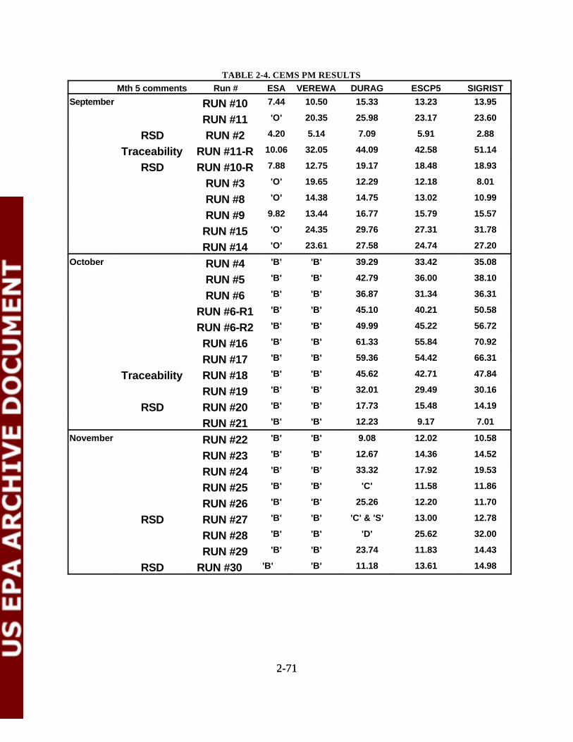
2-712-71

TABLE 2-4. CEMS PM RESULTSMth 5 comments Run # ESA VEREWA DURAG ESCP5 SIGRIST

September 7.44 10.50 15.33 13.23 13.95RUN #10RUN #11 'O' 20.35 25.98 23.17 23.60

RSD RUN #2 4.20 5.14 7.09 5.91 2.88

Traceability RUN #11-R 10.06 32.05 44.09 42.58 51.14

RSD RUN #10-R 7.88 12.75 19.17 18.48 18.93

RUN #3 'O' 19.65 12.29 12.18 8.01

RUN #8 'O' 14.38 14.75 13.02 10.99

RUN #9 9.82 13.44 16.77 15.79 15.57

RUN #15 'O' 24.35 29.76 27.31 31.78

RUN #14 'O' 23.61 27.58 24.74 27.20

October 'B' 'B' 39.29 33.42 35.08RUN #4RUN #5 'B' 'B' 42.79 36.00 38.10

RUN #6 'B' 'B' 36.87 31.34 36.31

RUN #6-R1 'B' 'B' 45.10 40.21 50.58

RUN #6-R2 'B' 'B' 49.99 45.22 56.72

RUN #16 'B' 'B' 61.33 55.84 70.92

RUN #17 'B' 'B' 59.36 54.42 66.31

Traceability RUN #18 'B' 'B' 45.62 42.71 47.84

RUN #19 'B' 'B' 32.01 29.49 30.16

RSD RUN #20 'B' 'B' 17.73 15.48 14.19

RUN #21 'B' 'B' 12.23 9.17 7.01

November 'B' 'B' 9.08 12.02 10.58RUN #22RUN #23 'B' 'B' 12.67 14.36 14.52

RUN #24 'B' 'B' 33.32 17.92 19.53

RUN #25 'B' 'B' 'C' 11.58 11.86

RUN #26 'B' 'B' 25.26 12.20 11.70

RSD RUN #27 'B' 'B' 'C' & 'S' 13.00 12.78

RUN #28 'B' 'B' 'D' 25.62 32.00

RUN #29 'B' 'B' 23.74 11.83 14.43

RSD RUN #30 'B' 'B' 11.18 13.61 14.98

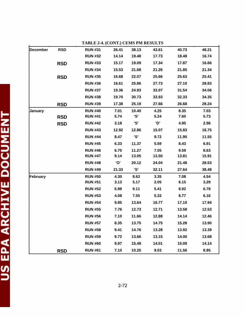
2-722-72

TABLE 2-4. (CONT.) CEMS PM RESULTSDecember RSD RUN #31 26.41 38.13 43.61 40.73 48.21

RUN #32 14.14 19.48 17.73 18.48 16.74

RSD RUN #33 15.17 19.09 17.34 17.87 16.66

RUN #34 15.53 21.68 21.26 21.85 21.34

RSD RUN #35 16.68 22.07 25.66 25.63 25.41

RUN #36 16.61 25.86 27.73 27.10 28.83

RUN #37 19.36 24.93 33.07 31.54 34.06

RUN #38 19.70 30.73 33.93 32.33 34.35

RSD RUN #39 17.38 25.19 27.66 26.68 28.24

January RUN #40 7.01 10.40 4.25 8.35 7.03

RSD RUN #41 5.74 'S' 5.24 7.60 5.73

RSD RUN #42 3.18 'S' 'D' 4.95 2.96

RUN #43 12.92 12.86 15.07 15.83 16.75

RUN #44 8.47 'S' 9.72 11.95 11.55

RUN #45 6.33 11.37 5.59 8.43 6.91

RUN #46 6.70 11.27 7.05 9.59 8.63RUN #47 9.14 13.05 13.50 13.81 15.91

RUN #48 'O' 20.12 24.04 21.48 28.53

RUN #49 21.33 'S' 32.11 27.64 38.48

February RUN #50 4.30 8.63 3.35 7.08 4.54RUN #51 3.13 5.17 2.05 6.15 3.29

RUN #52 5.98 9.11 5.41 8.92 6.78

RUN #53 4.08 7.55 5.33 8.77 6.16

RUN #54 9.85 13.64 16.77 17.10 17.94

RUN #55 7.76 12.73 12.71 13.58 12.53

RUN #56 7.10 11.66 12.88 14.14 12.46

RUN #57 8.35 13.75 14.75 15.28 13.90

RUN #58 9.41 14.76 13.28 13.92 13.39

RUN #59 9.72 13.66 13.15 14.00 13.68

RUN #60 9.97 15.49 14.01 15.09 14.14

RSD RUN #61 7.10 10.20 9.03 11.56 8.95

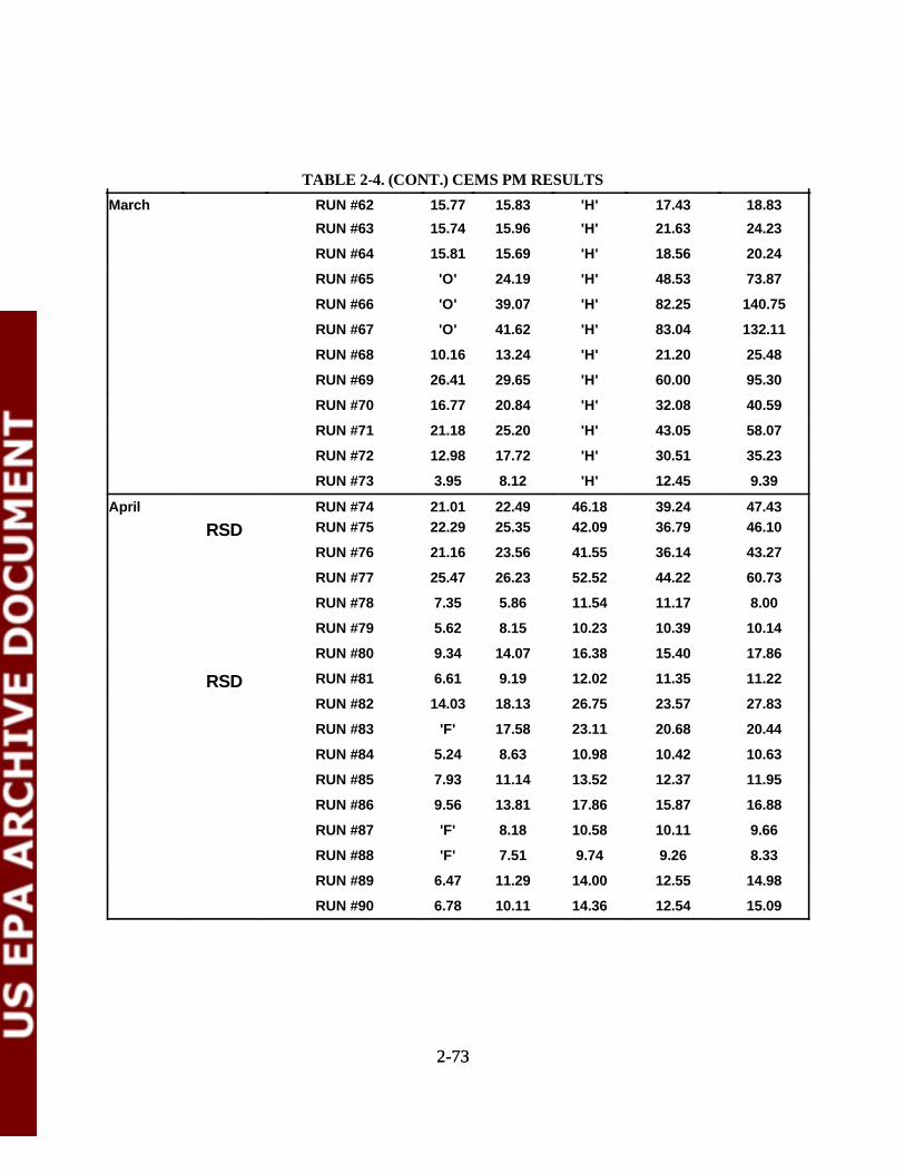
2-732-73

TABLE 2-4. (CONT.) CEMS PM RESULTSMarch RUN #62 15.77 15.83 'H' 17.43 18.83

RUN #63 15.74 15.96 'H' 21.63 24.23

RUN #64 15.81 15.69 'H' 18.56 20.24

RUN #65 'O' 24.19 'H' 48.53 73.87

RUN #66 'O' 39.07 'H' 82.25 140.75

RUN #67 'O' 41.62 'H' 83.04 132.11

RUN #68 10.16 13.24 'H' 21.20 25.48

RUN #69 26.41 29.65 'H' 60.00 95.30

RUN #70 16.77 20.84 'H' 32.08 40.59

RUN #71 21.18 25.20 'H' 43.05 58.07

RUN #72 12.98 17.72 'H' 30.51 35.23

RUN #73 3.95 8.12 'H' 12.45 9.39

April RUN #74 21.01 22.49 46.18 39.24 47.43

RSD RUN #75 22.29 25.35 42.09 36.79 46.10

RUN #76 21.16 23.56 41.55 36.14 43.27

RUN #77 25.47 26.23 52.52 44.22 60.73

RUN #78 7.35 5.86 11.54 11.17 8.00

RUN #79 5.62 8.15 10.23 10.39 10.14

RUN #80 9.34 14.07 16.38 15.40 17.86

RSD RUN #81 6.61 9.19 12.02 11.35 11.22

RUN #82 14.03 18.13 26.75 23.57 27.83

RUN #83 'F' 17.58 23.11 20.68 20.44

RUN #84 5.24 8.63 10.98 10.42 10.63

RUN #85 7.93 11.14 13.52 12.37 11.95

RUN #86 9.56 13.81 17.86 15.87 16.88

RUN #87 'F' 8.18 10.58 10.11 9.66

RUN #88 'F' 7.51 9.74 9.26 8.33

RUN #89 6.47 11.29 14.00 12.55 14.98

RUN #90 6.78 10.11 14.36 12.54 15.09

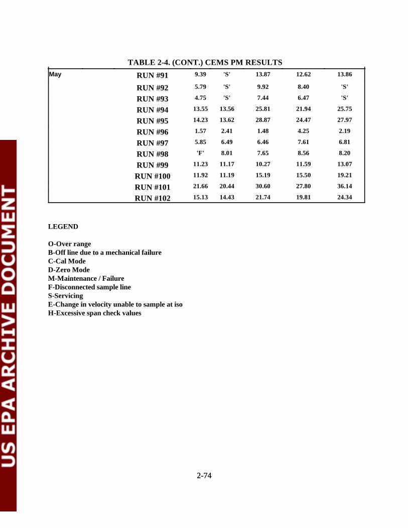
2-742-74

TABLE 2-4. (CONT.) CEMS PM RESULTSMay 9.39 'S' 13.87 12.62 13.86RUN #91

RUN #92 5.79 'S' 9.92 8.40 'S'

RUN #93 4.75 'S' 7.44 6.47 'S'

RUN #94 13.55 13.56 25.81 21.94 25.75

RUN #95 14.23 13.62 28.87 24.47 27.97

RUN #96 1.57 2.41 1.48 4.25 2.19

RUN #97 5.85 6.49 6.46 7.61 6.81

RUN #98 'F' 8.01 7.65 8.56 8.20

RUN #99 11.23 11.17 10.27 11.59 13.07

RUN #100 11.92 11.19 15.19 15.50 19.21

RUN #101 21.66 20.44 30.60 27.80 36.14

RUN #102 15.13 14.43 21.74 19.81 24.34

LEGEND

O-Over rangeB-Off line due to a mechanical failureC-Cal ModeD-Zero ModeM-Maintenance / FailureF-Disconnected sample lineS-ServicingE-Change in velocity unable to sample at isoH-Excessive span check values

2-752-75

TABLE 2-5. RESULTS OF LINEAR CALIBRATION RELATION

PERFORMANCE CRITERIA

CEM CALIBRATION SERIES Correlatio Confidence ToleranceProposed Emission Limitsn Coeffic Interval Interval

ient

mg/dscm @7% O2 (mg/Acm) Revised PS 11 > 0.90 < 10 % < 25 %

ESA Initial Calibration

max of cal. ( 20.97 ) 0.927 9.4% 15.8%

limit_50 ( 18.65 ) 17.1%8.8%slope = 7.3%0.824 limit_34 ( 12.68 ) 23.7%

Second Calibration

max of cal. ( 20.48 ) 0.985 7.1% 11.0%

limit_50 ( 18.1 ) 11.7%6.6%slope = 5.7%0.766 limit_34 ( 12.31 ) 15.5%

mg/dscm @7% O2 (mg/dscm)

VEREWA Initial Calibration

limit_69 ( 46 ) 10.6%6.1%limit_50 ( 33.33 ) 0.968 5.3% 13.9%

slope = 5.1%1.343 limit_34 ( 22.67 ) 20.0%

Second Calibration

max of cal. ( 34.92 ) 0.961 9.8% 15.7%

limit_50 ( 33.33 ) 16.4%9.6%slope = 8.0%1.430 limit_34 ( 22.67 ) 21.7%

mg/dscm @7% O2 (mg/Acm)

DURAG Initial Calibration

max of cal. ( 15.5 ) 0.952 8.2% 14.4%

slope = 7.2%0.421 limit_34 ( 12.44 ) 17.2%

Second Calibration

max of cal. ( 20.7 ) 0.972 8.7% 13.3%

limit_50 ( 18.1 ) 13.8%8.1%slope = 6.9%0.366 limit_34 ( 12.31 ) 18.8%

ESC Initial Calibration

limit_69 ( 25.73 ) 0.966 6.1% 11.1%

limit_50 ( 18.65 ) 14.7%5.3%slope = 0.357 limit_34 ( 12.68 ) 21.2%5.2%

Second Calibration

max of cal. ( 20.59 ) 0.978 7.8% 12.0%

limit_50 ( 18.1 ) 12.4%7.3%slope = 0.448 limit_34 ( 12.31 ) 16.9%6.2%

SIGRIST Initial Calibration

limit_69 ( 25.73 ) 0.936 8.5% 15.3%

limit_50 ( 18.65 ) 7.4% 19.9%

slope = 0.199 limit_34 ( 12.68 ) 28.7%7.1% A

Second Calibration

max of cal. ( 21.52 ) 0.951 12.0% A 17.0%

limit_50 ( 18.1 ) A 18.2%10.9%slope = 0.313 limit_34 ( 12.31 ) 24.9%9.2%

LEGENDA-Above performance specification criteriaMax of Cal. - PM Concentration Predicted by the Calibration Relation and the Maximum CEMS value

2-762-76

TABLE 2-6. CALIBRATION RANGE EFFECTS ON LINEAR REGRESSIONS

CEMS Slopes of Linear Regression Percent Difference in Slopes

A B C D A/B C/D A/D B/C

ESA 0.824 0.766 0.740 0.793 3.6% 3.5% 1.9% 1.7%

VEREWA 1.343 1.430 1.151 1.307 3.1% 6.3% 1.4% 10.8%

ESC 0.357 0.448 0.536 0.343 11.3% 21.9% 2.1% 8.9%

SIGRIST 0.199 0.313 0.389 0.193 22.2% 33.7% 1.6% 10.8%

LEGEND

A-Initial Calibration Original (December - March)B-Calibration 2 Original (April)C-Initial Calibration Rearranged (December - February)D-Calibration 2 Rearranged (April + March)

Percent Difference: [ x - x ] /xi ave ave

ESA was out of range 25% of MarchThis table does not apply to the DURAG.Excessive DURAG span check values in March produced unacceptable data during the entire March series.

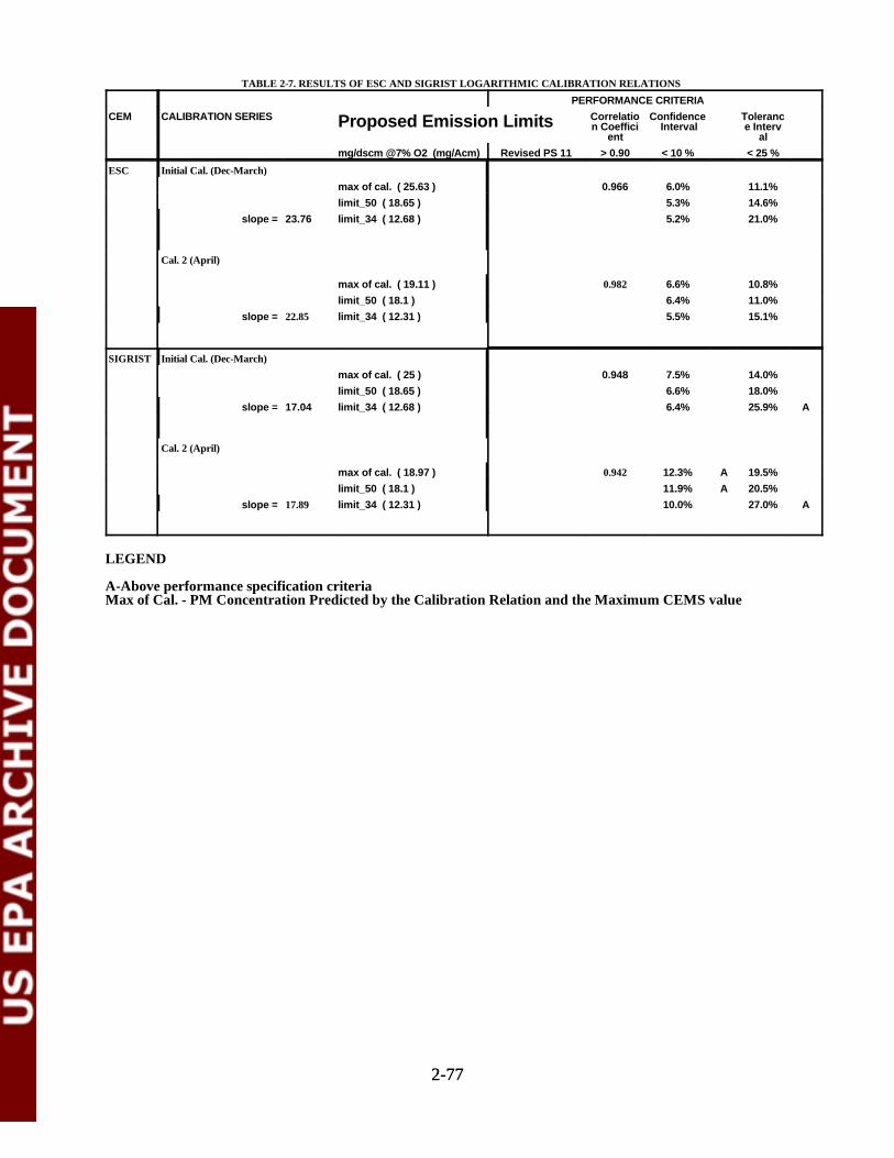
2-772-77

TABLE 2-7. RESULTS OF ESC AND SIGRIST LOGARITHMIC CALIBRATION RELATIONS

PERFORMANCE CRITERIACEM CALIBRATION SERIES Correlatio Confidence TolerancProposed Emission Limits n Coeffici Interval e Interv

ent almg/dscm @7% O2 (mg/Acm) Revised PS 11 > 0.90 < 10 % < 25 %

ESC Initial Cal. (Dec-March)max of cal. ( 25.63 ) 0.966 6.0% 11.1%limit_50 ( 18.65 ) 5.3% 14.6%

slope = 23.76 limit_34 ( 12.68 ) 5.2% 21.0%

Cal. 2 (April)

max of cal. ( 19.11 ) 0.982 6.6% 10.8%limit_50 ( 18.1 ) 6.4% 11.0%

slope = 22.85 limit_34 ( 12.31 ) 5.5% 15.1%

SIGRIST Initial Cal. (Dec-March)max of cal. ( 25 ) 0.948 7.5% 14.0%limit_50 ( 18.65 ) 6.6% 18.0%

slope = 17.04 limit_34 ( 12.68 ) 6.4% 25.9% A

Cal. 2 (April)

max of cal. ( 18.97 ) 0.942 12.3% A 19.5%limit_50 ( 18.1 ) 11.9% A 20.5%

slope = 17.89 limit_34 ( 12.31 ) 10.0% 27.0% A

LEGEND

A-Above performance specification criteriaMax of Cal. - PM Concentration Predicted by the Calibration Relation and the Maximum CEMS value

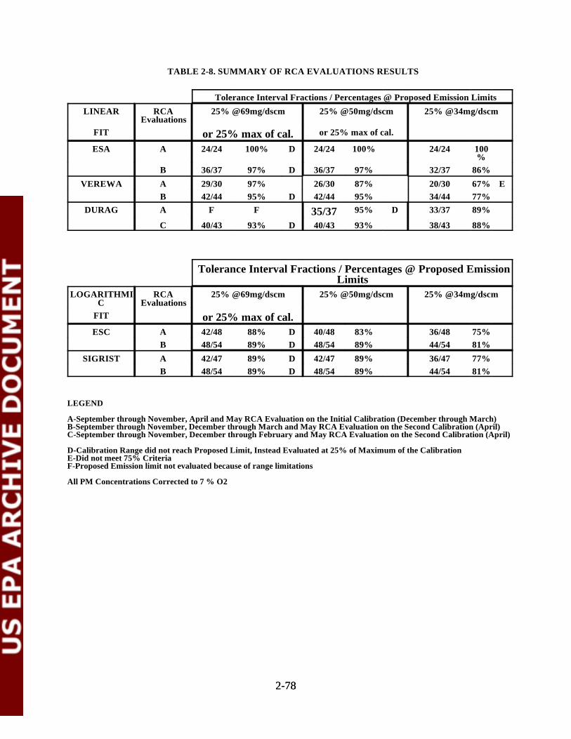
2-782-78

TABLE 2-8. SUMMARY OF RCA EVALUATIONS RESULTS

Tolerance Interval Fractions / Percentages @ Proposed Emission LimitsLINEAR RCA 25% @69mg/dscm 25% @50mg/dscm 25% @34mg/dscm

EvaluationsFIT or 25% max of cal.or 25% max of cal.ESA A 24/24 100% D 24/24 100% 24/24 100

%B 36/37 97% D 36/37 97% 32/37 86%

VEREWA A 29/30 97% 26/30 87% 20/30 67% EB 42/44 95% D 42/44 95% 34/44 77%

DURAG A F F 95% D 33/37 89%35/37C 40/43 93% D 40/43 93% 38/43 88%

Tolerance Interval Fractions / Percentages @ Proposed EmissionLimits

LOGARITHMI RCA 25% @69mg/dscm 25% @50mg/dscm 25% @34mg/dscmC Evaluations

FIT or 25% max of cal.ESC A 42/48 88% D 40/48 83% 36/48 75%

B 48/54 89% D 48/54 89% 44/54 81%SIGRIST A 42/47 89% D 42/47 89% 36/47 77%

B 48/54 89% D 48/54 89% 44/54 81%

LEGEND

A-September through November, April and May RCA Evaluation on the Initial Calibration (December through March)B-September through November, December through March and May RCA Evaluation on the Second Calibration (April)C-September through November, December through February and May RCA Evaluation on the Second Calibration (April)

D-Calibration Range did not reach Proposed Limit, Instead Evaluated at 25% of Maximum of the CalibrationE-Did not meet 75% CriteriaF-Proposed Emission limit not evaluated because of range limitations

All PM Concentrations Corrected to 7 % O2

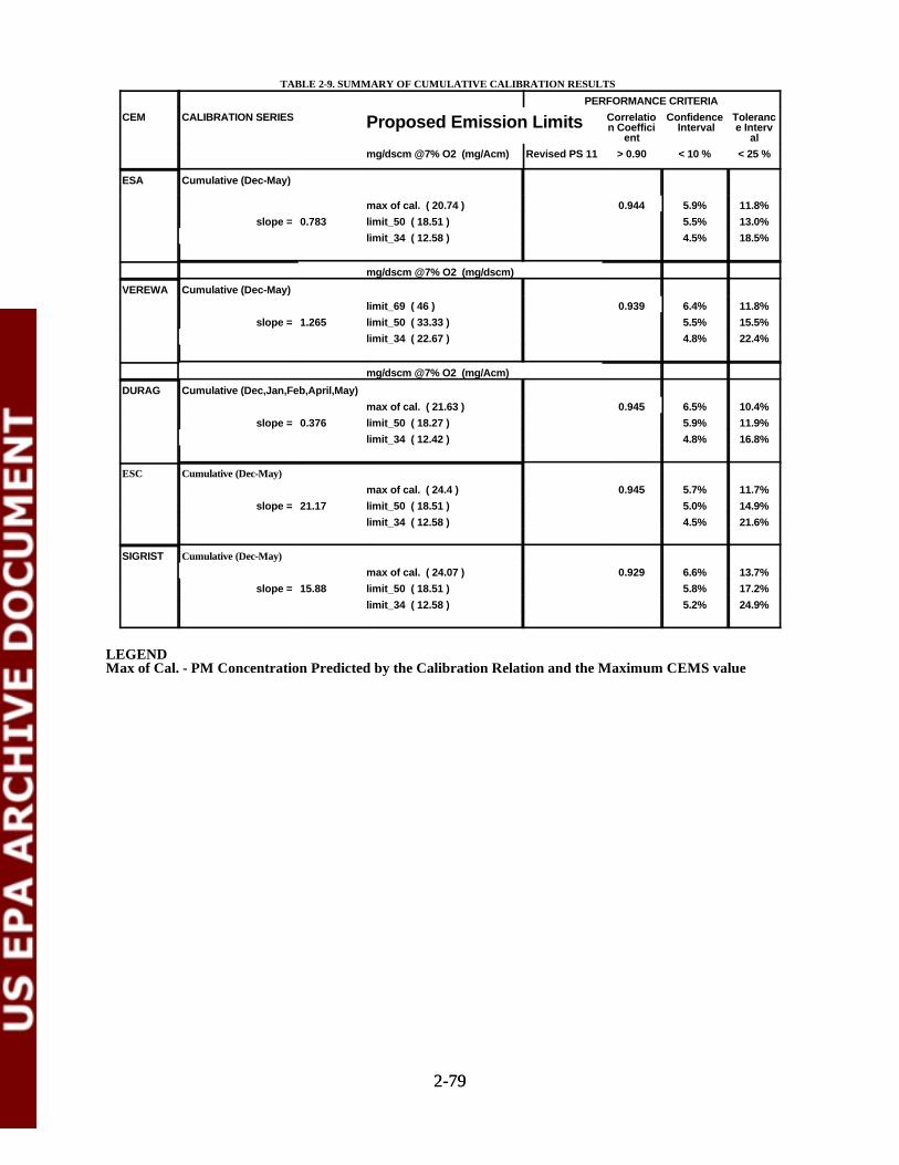
2-792-79

TABLE 2-9. SUMMARY OF CUMULATIVE CALIBRATION RESULTS

PERFORMANCE CRITERIACEM CALIBRATION SERIES Correlatio Confidence TolerancProposed Emission Limits n Coeffici Interval e Interv

ent almg/dscm @7% O2 (mg/Acm) Revised PS 11 > 0.90 < 10 % < 25 %

ESA Cumulative (Dec-May)

max of cal. ( 20.74 ) 0.944 5.9% 11.8%slope = 0.783 limit_50 ( 18.51 ) 5.5% 13.0%

limit_34 ( 12.58 ) 4.5% 18.5%

mg/dscm @7% O2 (mg/dscm)

VEREWA Cumulative (Dec-May)limit_69 ( 46 ) 0.939 6.4% 11.8%

slope = 1.265 limit_50 ( 33.33 ) 5.5% 15.5%limit_34 ( 22.67 ) 4.8% 22.4%

mg/dscm @7% O2 (mg/Acm)

DURAG Cumulative (Dec,Jan,Feb,April,May)max of cal. ( 21.63 ) 0.945 6.5% 10.4%

slope = 0.376 limit_50 ( 18.27 ) 5.9% 11.9%limit_34 ( 12.42 ) 4.8% 16.8%

ESC Cumulative (Dec-May)max of cal. ( 24.4 ) 0.945 5.7% 11.7%

slope = 21.17 limit_50 ( 18.51 ) 5.0% 14.9%limit_34 ( 12.58 ) 4.5% 21.6%

SIGRIST Cumulative (Dec-May)max of cal. ( 24.07 ) 0.929 6.6% 13.7%

slope = 15.88 limit_50 ( 18.51 ) 5.8% 17.2%limit_34 ( 12.58 ) 5.2% 24.9%

LEGENDMax of Cal. - PM Concentration Predicted by the Calibration Relation and the Maximum CEMS value

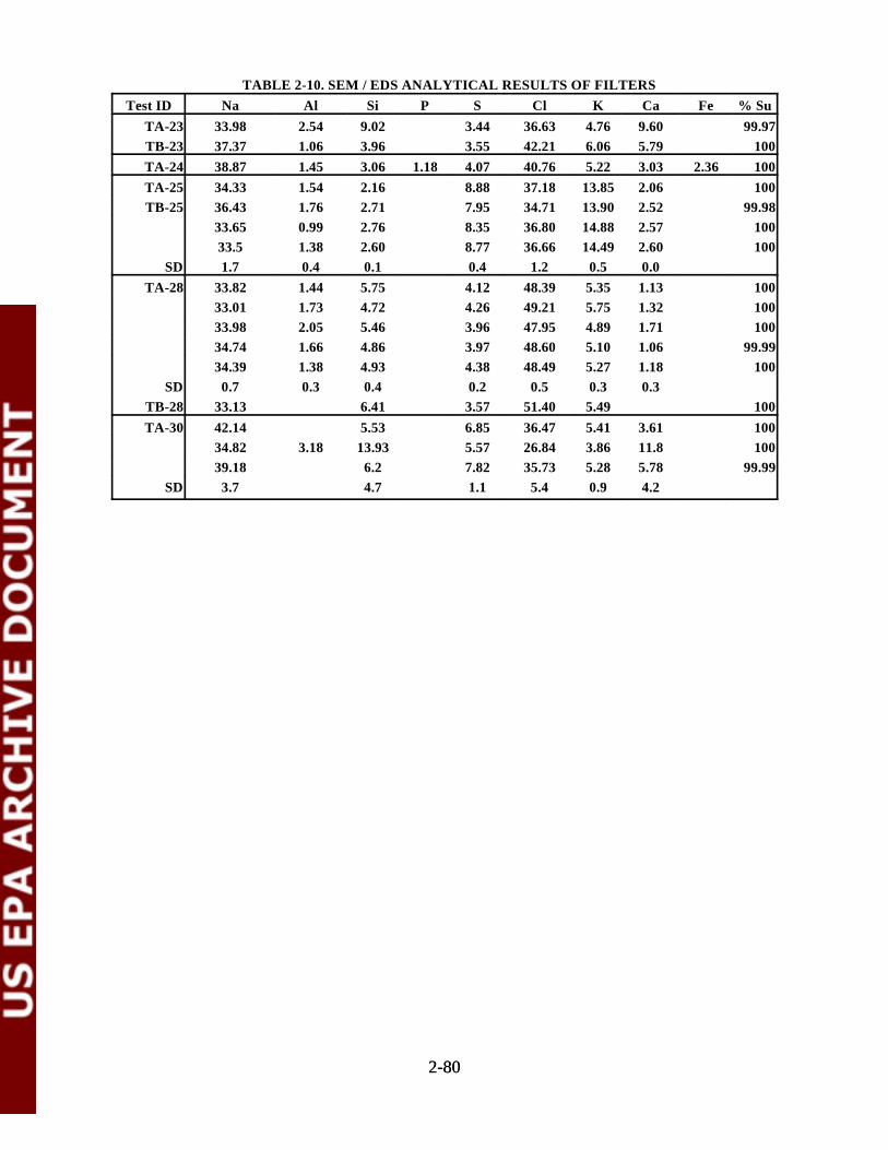
2-802-80

TABLE 2-10. SEM / EDS ANALYTICAL RESULTS OF FILTERSTest ID Na Al Si P S Cl K Ca Fe % Su

TA-23 33.98 2.54 9.02 3.44 36.63 4.76 9.60 99.97TB-23 37.37 1.06 3.96 3.55 42.21 6.06 5.79 100TA-24 38.87 1.45 3.06 1.18 4.07 40.76 5.22 3.03 2.36 100TA-25 34.33 1.54 2.16 8.88 37.18 13.85 2.06 100TB-25 36.43 1.76 2.71 7.95 34.71 13.90 2.52 99.98

33.65 0.99 2.76 8.35 36.80 14.88 2.57 10033.5 1.38 2.60 8.77 36.66 14.49 2.60 100

SD 1.7 0.4 0.1 0.4 1.2 0.5 0.0TA-28 33.82 1.44 5.75 4.12 48.39 5.35 1.13 100

33.01 1.73 4.72 4.26 49.21 5.75 1.32 10033.98 2.05 5.46 3.96 47.95 4.89 1.71 10034.74 1.66 4.86 3.97 48.60 5.10 1.06 99.9934.39 1.38 4.93 4.38 48.49 5.27 1.18 100

SD 0.7 0.3 0.4 0.2 0.5 0.3 0.3TB-28 33.13 6.41 3.57 51.40 5.49 100TA-30 42.14 5.53 6.85 36.47 5.41 3.61 100

34.82 3.18 13.93 5.57 26.84 3.86 11.8 10039.18 6.2 7.82 35.73 5.28 5.78 99.99

SD 3.7 4.7 1.1 5.4 0.9 4.2

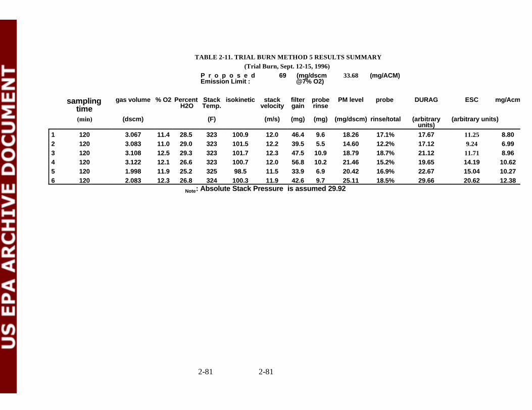
2-81 2-81

TABLE 2-11. TRIAL BURN METHOD 5 RESULTS SUMMARY(Trial Burn, Sept. 12-15, 1996)

P r o p o s e d 69 (mg/dscm 33.68 (mg/ACM)Emission Limit : @7% O2)

samplingtime

gas volume % O2 Percent Stack isokinetic stack filter probe PM level probe DURAG ESC mg/Acm H2O Temp. velocity gain rinse

(min) (dscm) (F) (m/s) (mg) (mg) (mg/dscm) rinse/total (arbitrary (arbitrary units)units)

1 120 3.067 11.4 28.5 323 100.9 12.0 46.4 9.6 18.26 17.1% 17.67 11.25 8.802 120 3.083 11.0 29.0 323 101.5 12.2 39.5 5.5 14.60 12.2% 17.12 9.24 6.993 120 3.108 12.5 29.3 323 101.7 12.3 47.5 10.9 18.79 18.7% 21.12 11.71 8.964 120 3.122 12.1 26.6 323 100.7 12.0 56.8 10.2 21.46 15.2% 19.65 14.19 10.625 120 1.998 11.9 25.2 325 98.5 11.5 33.9 6.9 20.42 16.9% 22.67 15.04 10.276 120 2.083 12.3 26.8 324 100.3 11.9 42.6 9.7 25.11 18.5% 29.66 20.62 12.38

Note: Absolute Stack Pressure is assumed 29.92

2-822-82

TABLE 2-12. PM CEMS DATA DURING TRIAL BURN

DATE RUN # CEM ID AVERAGE MGM

9/12/96 1 DURAG 17.67ESA Data suspect

ESCP5 11.25SIGRIST No dataVEREWA Data suspect

9/13/96 2 DURAG 17.12ESA Data suspect

ESCP5 9.24SIGRIST No dataVEREWA Data suspect

9/13/96 3 DURAG 21.12ESA Data suspect

ESCP5 11.71SIGRIST No dataVEREWA Data suspect

9/14/96 4 DURAG 19.65ESA Data suspect

ESCP5 14.19SIGRIST No dataVEREWA Data suspect

9/15/96 5 DURAG 22.67ESA Data suspect

ESCP5 15.04SIGRIST No dataVEREWA Data suspect

9/15/96 6 DURAG 29.66ESA Data suspect

ESCP5 20.62SIGRIST No dataVEREWA Data suspect

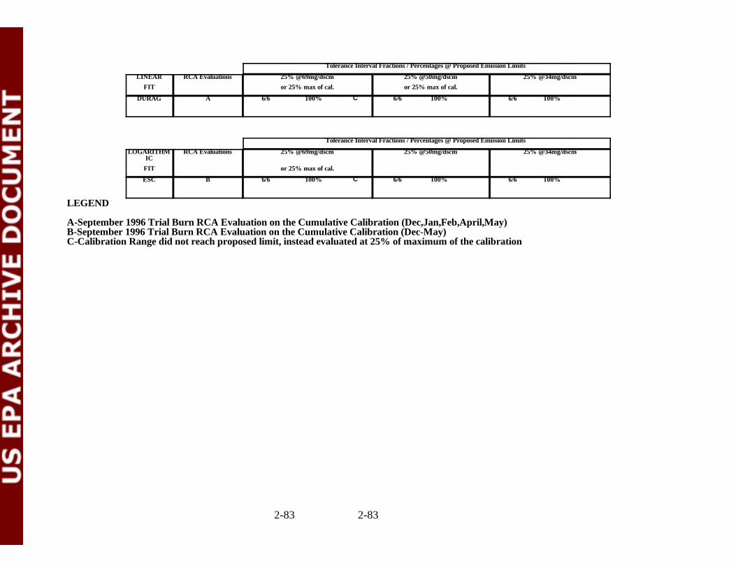
2-83 2-83

Tolerance Interval Fractions / Percentages @ Proposed Emission Limits

LINEAR RCA Evaluations 25% @69mg/dscm 25% @50mg/dscm 25% @34mg/dscmFIT or 25% max of cal. or 25% max of cal.

DURAG A 6/6 100% C 6/6 100% 6/6 100%

Tolerance Interval Fractions / Percentages @ Proposed Emission Limits

LOGARITHMIC

RCA Evaluations 25% @69mg/dscm 25% @50mg/dscm 25% @34mg/dscm

FIT or 25% max of cal.

ESC B 6/6 100% C 6/6 100% 6/6 100%

LEGEND

A-September 1996 Trial Burn RCA Evaluation on the Cumulative Calibration (Dec,Jan,Feb,April,May)B-September 1996 Trial Burn RCA Evaluation on the Cumulative Calibration (Dec-May)C-Calibration Range did not reach proposed limit, instead evaluated at 25% of maximum of the calibration

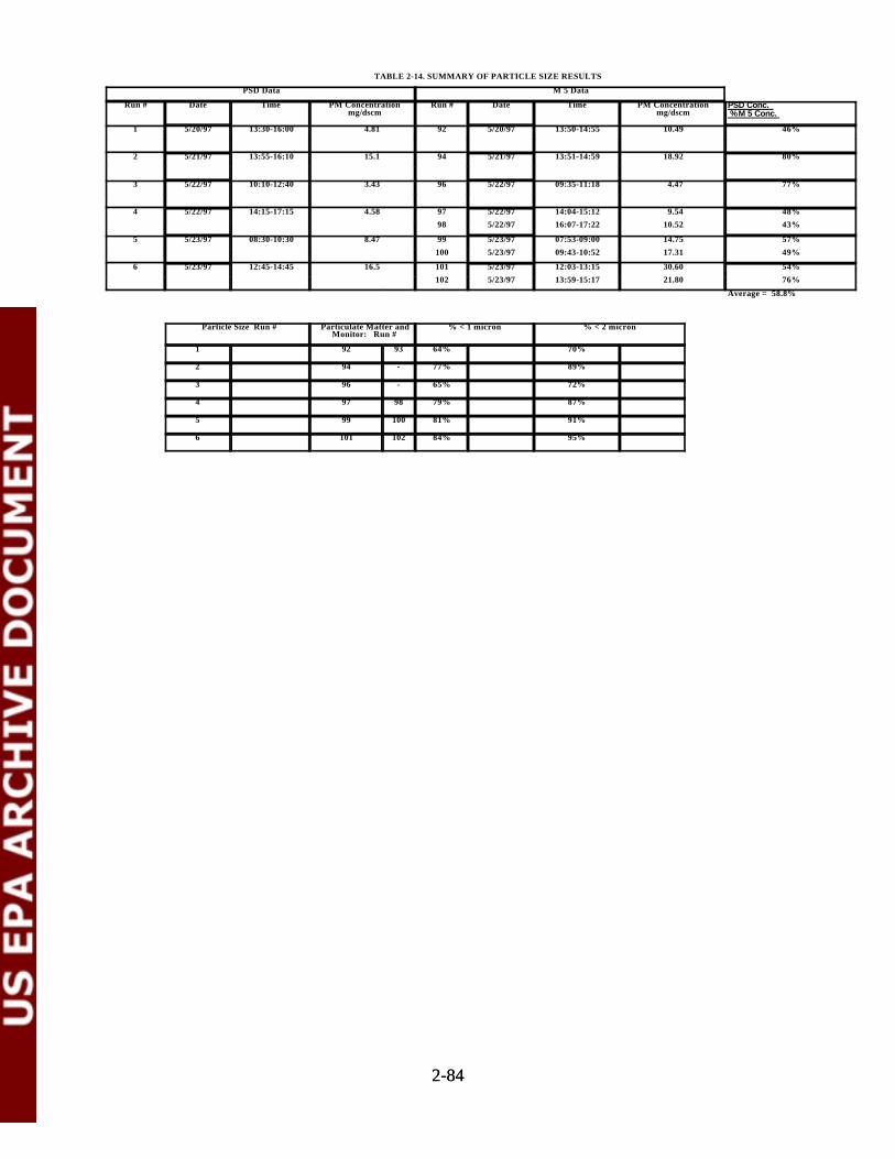
2-842-84

TABLE 2-14. SUMMARY OF PARTICLE SIZE RESULTS

PSD Data M 5 Data

Run # Date Time PM Concentration mg/dscm

Run # Date Time PM Concentration mg/dscm

PSD Conc. % M 5 Conc.

1 5/20/97 13:30-16:00 4.81 92 5/20/97 13:50-14:55 10.49 46%

2 5/21/97 13:55-16:10 15.1 94 5/21/97 13:51-14:59 18.92 80%

3 5/22/97 10:10-12:40 3.43 96 5/22/97 09:35-11:18 4.47 77%

4 5/22/97 14:15-17:15 4.58 97 5/22/97 14:04-15:12 9.54 48%98 5/22/97 16:07-17:22 10.52 43%

5 5/23/97 08:30-10:30 8.47 99 5/23/97 07:53-09:00 14.75 57%100 5/23/97 09:43-10:52 17.31 49%

6 5/23/97 12:45-14:45 16.5 101 5/23/97 12:03-13:15 30.60 54%102 5/23/97 13:59-15:17 21.80 76%

Average = 58.8%

Particle Size Run # Particulate Matter andMonitor: Run #

% < 1 micron % < 2 micron

1 92 93 64% 70%

2 94 - 77% 89%

3 96 - 65% 72%

4 97 98 79% 87%

5 99 100 81% 91%

6 101 102 84% 95%

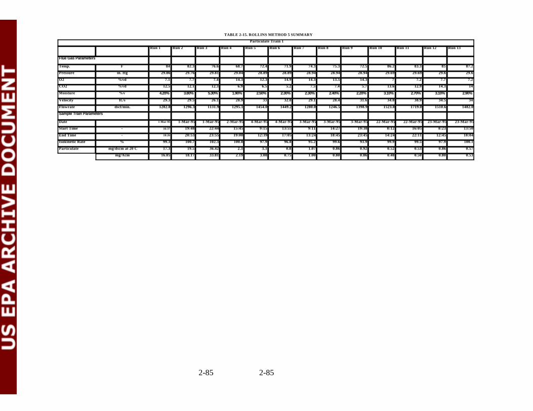
2-85 2-85

TABLE 2-15. ROLLINS METHOD 5 SUMMARY

Particulate Train 1

Run 1 Run 2 Run 3 Run 4 Run 5 Run 6 Run 7 Run 8 Run 9 Run 10 Run 11 Run 12 Run 13

Flue Gas Parameters

Temp. F 84 82.3 76.6 68.7 72.4 71.9 74.3 75.3 72.5 86.2 83.3 85 87.2

Pressure in. Hg 29.86 29.76 29.81 29.04 28.89 28.89 28.94 28.94 28.94 29.69 29.69 29.6 29.6

O2 %vd 7.1 7.7 7.4 14.3 12.3 14.9 14.3 13.5 14.3 7 7.2 7.7 7.2

CO2 %vd 12.5 12.1 12.3 6.9 6.5 5.2 7.5 7.4 5.7 13.6 12.9 14.3 14

Moisture %v 4.20% 3.80% 5.30% 1.90% 2.50% 2.30% 2.30% 2.40% 2.20% 3.10% 2.70% 3.10% 2.90%

Velocity ft./s 29.3 29.5 26.1 28.9 33 32.8 29.1 28.4 31.6 34.8 38.9 34.5 34

Flowrate dscf/min. 1282.8 1296.3 1131.9 1295.1 1454.0 1449.2 1280.0 1246.5 1398.9 1523.8 1719.0 1510.6 1482.0

Sample Train Parameters

Date 1-Mar-95 1-Mar-95 1-Mar-95 2-Mar-95 4-Mar-95 4-Mar-95 3-Mar-95 3-Mar-95 3-Mar-95 22-Mar-95 22-Mar-95 23-Mar-95 23-Mar-95

Start Time - 16:37 19:48 22:44 15:45 9:15 13:55 9:11 14:27 19:38 8:12 16:05 8:23 13:50

End Time - 18:26 20:53 23:55 19:00 12:39 17:05 13:24 18:45 23:45 14:24 22:11 12:45 18:04

Isokinetic Rate % 99.3 100.7 102.3 100.8 97.9 96.8 95.2 99.6 93.9 99.9 99.5 97.9 100.1

Particulate mg/dscm at 20 C 17.3 19.5 36.42 2.3 3.3 0.8 1.07 0.86 0.92 0.52 0.53 0.86 0.57

mg/Acm 16.05 18.17 33.81 2.19 3.08 0.75 1.00 0.80 0.86 0.48 0.50 0.80 0.53

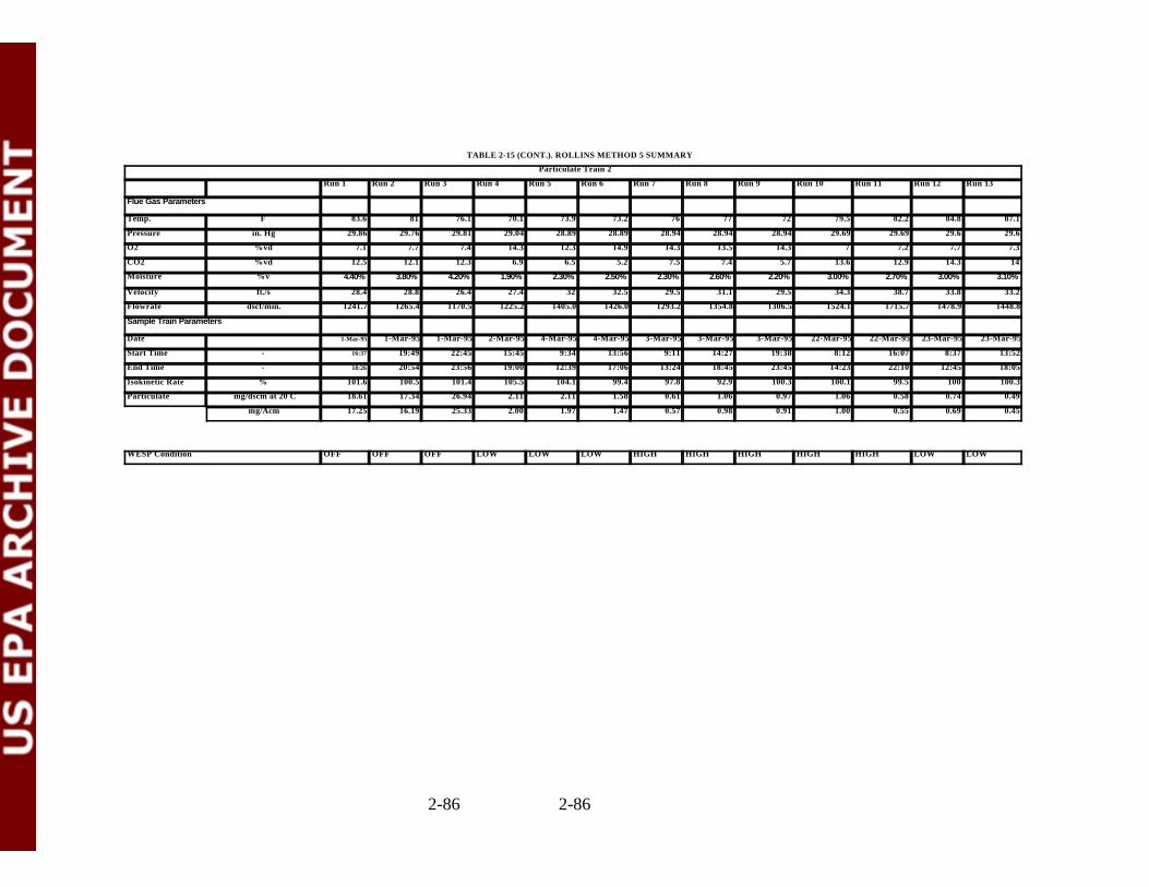
2-86 2-86

TABLE 2-15 (CONT.). ROLLINS METHOD 5 SUMMARY

Particulate Train 2

Run 1 Run 2 Run 3 Run 4 Run 5 Run 6 Run 7 Run 8 Run 9 Run 10 Run 11 Run 12 Run 13

Flue Gas Parameters

Temp. F 83.6 81 76.1 70.1 73.9 73.2 76 77 72 79.5 82.2 84.8 87.1

Pressure in. Hg 29.86 29.76 29.81 29.04 28.89 28.89 28.94 28.94 28.94 29.69 29.69 29.6 29.6

O2 %vd 7.1 7.7 7.4 14.3 12.3 14.9 14.3 13.5 14.3 7 7.2 7.7 7.3

CO2 %vd 12.5 12.1 12.3 6.9 6.5 5.2 7.5 7.4 5.7 13.6 12.9 14.3 14

Moisture %v 4.40% 3.80% 4.20% 1.90% 2.30% 2.50% 2.30% 2.60% 2.20% 3.00% 2.70% 3.00% 3.10%

Velocity ft./s 28.4 28.8 26.4 27.4 32 32.5 29.5 31.1 29.5 34.3 38.7 33.8 33.2

Flowrate dscf/min. 1241.7 1265.4 1170.5 1225.2 1405.0 1426.0 1293.2 1354.8 1306.5 1524.1 1715.7 1478.9 1448.8

Sample Train Parameters

Date 1-Mar-95 1-Mar-95 1-Mar-95 2-Mar-95 4-Mar-95 4-Mar-95 3-Mar-95 3-Mar-95 3-Mar-95 22-Mar-95 22-Mar-95 23-Mar-95 23-Mar-95

Start Time - 16:37 19:49 22:45 15:45 9:34 13:56 9:11 14:27 19:38 8:12 16:07 8:37 13:52

End Time - 18:26 20:54 23:56 19:00 12:39 17:06 13:24 18:45 23:45 14:23 22:10 12:45 18:05

Isokinetic Rate % 101.6 100.5 101.4 105.5 104.1 99.4 97.8 92.9 100.3 100.1 99.5 100 100.3

Particulate mg/dscm at 20 C 18.61 17.34 26.94 2.11 2.11 1.58 0.61 1.06 0.97 1.06 0.58 0.74 0.49

mg/Acm 17.25 16.19 25.33 2.00 1.97 1.47 0.57 0.98 0.91 1.00 0.55 0.69 0.45

WESP Condition OFF OFF OFF LOW LOW LOW HIGH HIGH HIGH HIGH HIGH LOW LOW

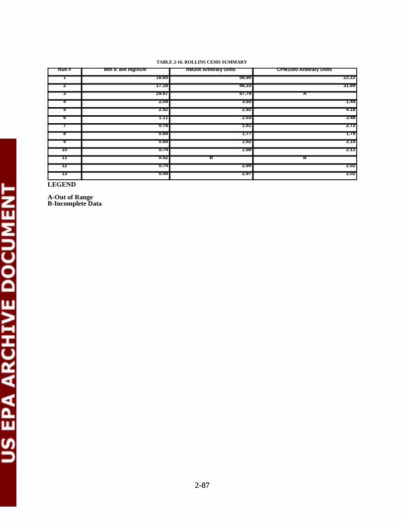
2-872-87

TABLE 2-16. ROLLINS CEMS SUMMARY

Run # Mth 5: ave mg/Acm RM200 Arbitrary Units CPM1000 Arbitrary Units

1 16.65 58.94 22.22

2 17.18 46.33 31.99

3 29.57 57.79 A

4 2.09 3.50 1.44

5 2.52 2.92 4.18

6 1.11 2.03 3.48

7 0.78 1.51 2.72

8 0.89 1.77 1.79

9 0.89 1.52 2.15

10 0.74 1.58 2.11

11 0.52 B B

12 0.74 2.94 2.02

13 0.49 2.97 2.02

LEGEND

A-Out of RangeB-Incomplete Data

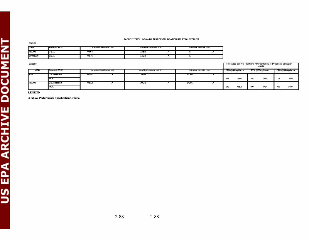
2-88 2-88

TABLE 2-17 ROLLINS AND LAFARGE CALIBRATION RELATION RESULTS

Rollins

CEM Revised PS 11 Correlation Coefficient > 0.90 Confidence Interval << 10 % Tolerance Interval < 25 %

RM200 Cal. 1 0.953 18.5% A A A

CPM1000 Cal. 1 0.976 14.2% A A

Lafarge Tolerance Interval Fractions / Percentages @ Proposed EmissionLimits

CEM Revised PS 11 Correlation Coefficient > 0.90 Confidence Interval < 10 % Tolerance Interval < 25 % 25% @69mg/dscm 25% @50mg/dscm 25% @34mg/dscm

P5A Cal. Relation 0.792 A 16.6% 36.5% A

RCA 5/8 63% 3/8 38% 2/8 25%

RM200 Cal. Relation 0.512 A 30.2% A 54.9% A

RCA 0/0 #N/A 0/0 #N/A 0/0 #N/A

LEGEND

A-Above Performance Specification Criteria

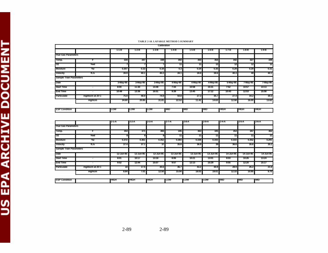
2-89 2-89

TABLE 2-18. LAFARGE METHOD 5 SUMMARY

Calibration

1-1-B 1-2-B 1-3-B 1-4-B 1-5-B 1-6-B 1-7-B 1-8-B 1-9-B

Flue Gas Parameters

Temp. F 334 347 338 350 350 354 342 327 336

O2 %vd 7 7 7 11 11 12 12 12 12

Moisture %v 0.307 0.33 0.34 0.3 0.34 0.35 0.29 0.29 0.31

Velocity ft./s 39.9 40.1 40.2 39.1 39.8 39.6 40.3 40 40.1

Sample Train Parameters

Date 3-May-95 3-May-95 3-May-95 4-May-95 4-May-95 4-May-95 5-May-95 7-May-95 7-May-95

Start Time - 8:00 11:30 14:48 7:44 10:58 15:31 7:52 10:57 14:13

End Time - 10:48 13:36 16:51 9:39 13:45 17:12 10:43 12:53 15:58

Particulate mg/dscm at 20 C 75.9 48.9 74.9 50.8 27.3 35.7 27.4 34.2 30.3

mg/Acm 34.60 20.85 31.81 22.53 11.42 14.63 12.58 16.00 13.62

ESP Condition LOW LOW LOW MID MID MID HIGH HIGH HIGH

2-1-A 2-2-A 2-3-A 2-7-A 2-8-A 2-9-A 2-4-A 2-5-A 2-6-A

Flue Gas Parameters

Temp. F 354 371 366 345 363 345 354 347 362

O2 %vd 8 8 8 11 11 11 11 11 11

Moisture %v 0.372 0.361 0.352 0.364 0.338 0.343 0.333 0.352 0.291

Velocity ft./s 37.4 37.1 37 35.6 36.9 39 36.6 35.6 35.2

Sample Train Parameters

Date 12-Jun-95 12-Jun-95 12-Jun-95 13-Jun-95 13-Jun-95 13-Jun-95 14-Jun-95 14-Jun-95 14-Jun-95

Start Time - 8:01 10:17 13:18 8:06 10:21 13:01 8:03 10:26 13:24

End Time - 9:52 12:44 15:07 9:57 12:13 15:29 9:55 12:20 15:17

Particulate mg/dscm at 20 C 22 17.5 30.6 36.7 43.2 44.9 28.9 26.2 21.6

mg/Acm 8.84 7.01 12.50 15.04 18.03 19.01 12.33 10.95 9.70

ESP Condition HIGH HIGH HIGH LOW LOW LOW MID MID MID

2-90 2-90

TABLE 2-18 (CONT.). LAFARGE METHOD 5 SUMMARY

RCA

Train A

3-1 3-2 3-3 3-4 3-5 3-6 3-7 3-8 3-9

Flue Gas Parameters

Temp. F 342 342 342 335 331 344 344 345 345

O2 %vd 7 7 7 7 7 7 7 7 7

Moisture %v 0.28 0.30 0.31 0.29 0.30 0.30 0.30 0.31 0.31

Velocity ft./s 43.8 45.3 42.6 44.3 45.3 45.2 44.6 45.3 44.9

Sample Train Parameters

Date 18-Jul-95 18-Jul-95 18-Jul-95 19-Jul-95 19-Jul-95 19-Jul-95 19-Jul-95 19-Jul-95 19-Jul-95

Start Time - 14:37 17:30 9:58 9:51 12:05 14:24 17:30 19:46 23:00

End Time - 16:37 19:25 21:48 11:34 13:38 16:08 19:04 22:11 24:33

Particulate mg/dscm at 20 C 28.53 31.79 25.89 32.38 40.83 34.83 31.15 37.54 33.63

mg/Acm 12.92 14.30 11.58 15.19 18.95 16.00 14.26 17.09 15.23

Train B

3-1 3-2 3-3 3-4 3-5 3-6 3-7 3-8 3-9

Flue Gas Parameters

Temp. F 343 341 341 343 339 344 342 343 342

O2 %vd 7 7 7 7 7 7 7 7 7

Moisture %v 0.30 0.31 0.31 0.31 0.31 0.32 0.31 0.32 0.31

Velocity ft./s 43.6 43.6 45.6 43.2 45.7 44.3 45.1 45.2 45.2

Sample Train Parameters

Date 18-Jul-95 18-Jul-95 18-Jul-95 19-Jul-95 19-Jul-95 19-Jul-95 19-Jul-95 19-Jul-95 19-Jul-95

Start Time - 14:42 17:31 20:39 9:53 12:05 14:24 17:30 19:42 22:57

End Time - 16:53 19:25 22:31 11:33 13:43 16:09 19:06 22:06 24:24

Particulate mg/dscm at 20 C 27.69 27.92 25.64 36.50 37.12 37.04 29.02 36.85 31.59

mg/Acm 13.16 12.85 11.62 16.28 16.63 16.37 12.91 16.36 14.23

ESP Condition HIGH HIGH HIGH LOW LOW LOW MID MID MID

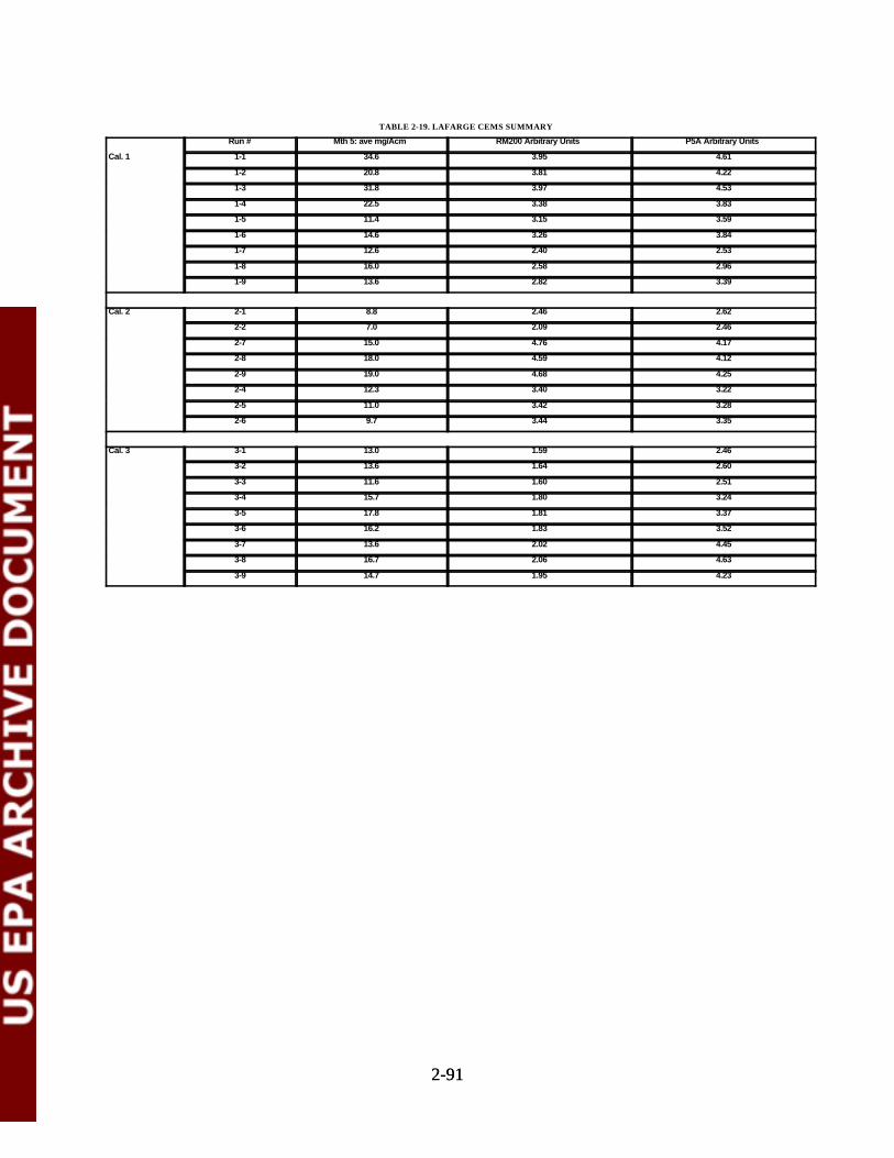
2-912-91

TABLE 2-19. LAFARGE CEMS SUMMARY

Run # Mth 5: ave mg/Acm RM200 Arbitrary Units P5A Arbitrary Units

Cal. 1 1-1 34.6 3.95 4.61

1-2 20.8 3.81 4.22

1-3 31.8 3.97 4.53

1-4 22.5 3.38 3.83

1-5 11.4 3.15 3.59

1-6 14.6 3.26 3.84

1-7 12.6 2.40 2.53

1-8 16.0 2.58 2.96

1-9 13.6 2.82 3.39

Cal. 2 2-1 8.8 2.46 2.62

2-2 7.0 2.09 2.46

2-7 15.0 4.76 4.17

2-8 18.0 4.59 4.12

2-9 19.0 4.68 4.25

2-4 12.3 3.40 3.22

2-5 11.0 3.42 3.28

2-6 9.7 3.44 3.35

Cal. 3 3-1 13.0 1.59 2.46

3-2 13.6 1.64 2.60

3-3 11.6 1.60 2.51

3-4 15.7 1.80 3.24

3-5 17.8 1.81 3.37

3-6 16.2 1.83 3.52

3-7 13.6 2.02 4.45

3-8 16.7 2.06 4.63

3-9 14.7 1.95 4.23

2-922-92

TABLE 2-20. PM CEMS COST ESTIMATE SUMMARY(All costs in thousands of dollars)

PM CEMS Technology with Monitor Total Capital Total Annual Totalsampling and analysis Costs ($) Cost ($) Cost ($/year) Annualizedcharacteristics Cost ($/year)

Beta-gauge CEMS with heated 46 125 24 42extractive sampling andexternal analysis

In-situ light-scattering CEMS 13 120 13 30

Extractive light-scattering 66 175 21 46CEMS heated with externalanalysis

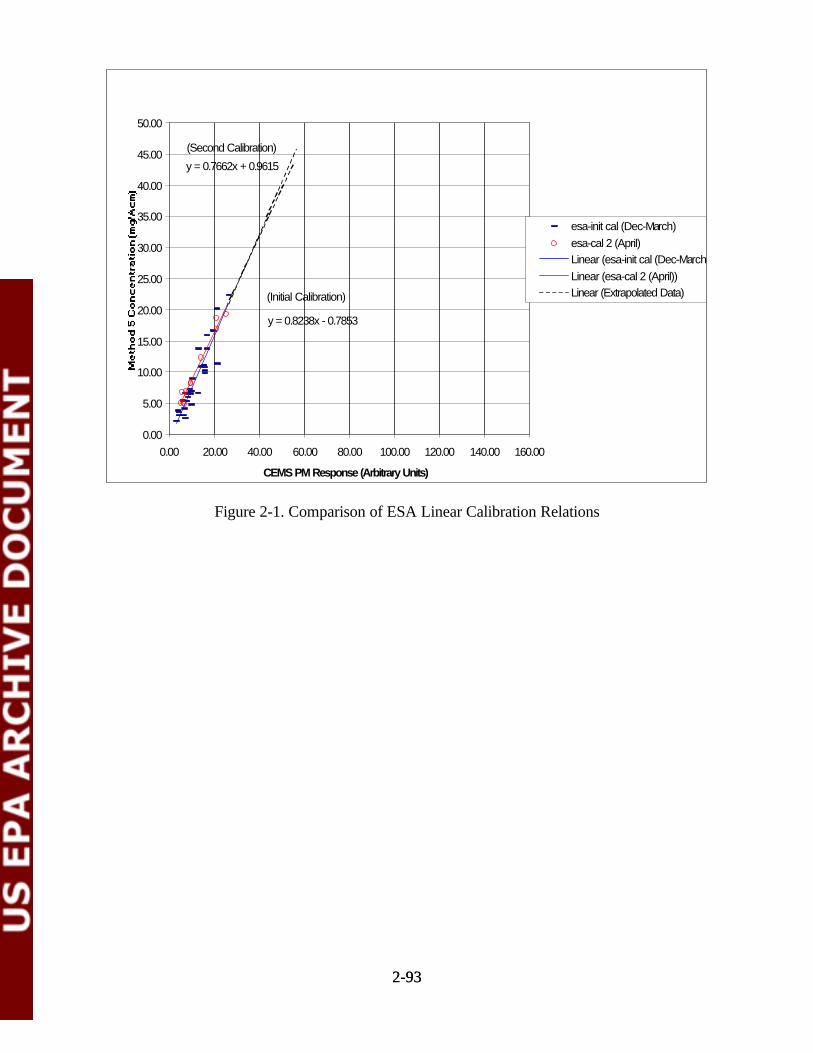
y = 0.8238x - 0.7853

y = 0.7662x + 0.9615

0.00

5.00

10.00

15.00

20.00

25.00

30.00

35.00

40.00

45.00

50.00

0.00 20.00 40.00 60.00 80.00 100.00 120.00 140.00 160.00

CEMS PM Response (Arbitrary Units)

esa-init cal (Dec-March)esa-cal 2 (April)Linear (esa-init cal (Dec-March))Linear (esa-cal 2 (April))Linear (Extrapolated Data)(Initial Calibration)

(Second Calibration)

2-932-93

Figure 2-1. Comparison of ESA Linear Calibration Relations

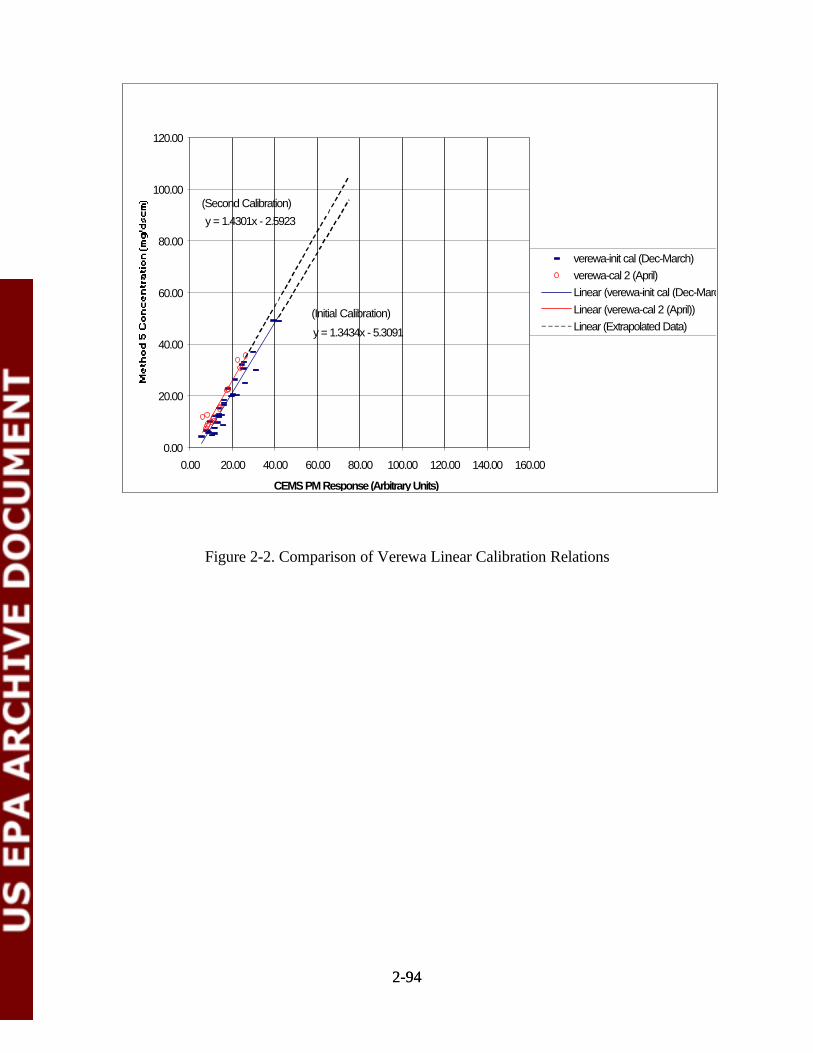
y = 1.3434x - 5.3091

y = 1.4301x - 2.5923

0.00

20.00

40.00

60.00

80.00

100.00

120.00

0.00 20.00 40.00 60.00 80.00 100.00 120.00 140.00 160.00

CEMS PM Response (Arbitrary Units)

verewa-init cal (Dec-March)verewa-cal 2 (April)Linear (verewa-init cal (Dec-March))Linear (verewa-cal 2 (April))Linear (Extrapolated Data)

(Initial Calibration)

(Second Calibration)

2-942-94

Figure 2-2. Comparison of Verewa Linear Calibration Relations

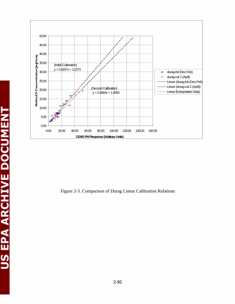
y = 0.4207x + 1.2273

y = 0.3664x + 1.4559

0.00

5.00

10.00

15.00

20.00

25.00

30.00

35.00

40.00

45.00

50.00

0.00 20.00 40.00 60.00 80.00 100.00 120.00 140.00 160.00

CEMS PM Response (Arbitrary Units)

durag-init (Dec-Feb)durag-cal 2 (April)Linear (durag-init (Dec-Feb))Linear (durag-cal 2 (April))Linear (Extrapolated Data)

(Initial Calibration)

(Second Calibration)

2-952-95

Figure 2-3. Comparison of Durag Linear Calibration Relations

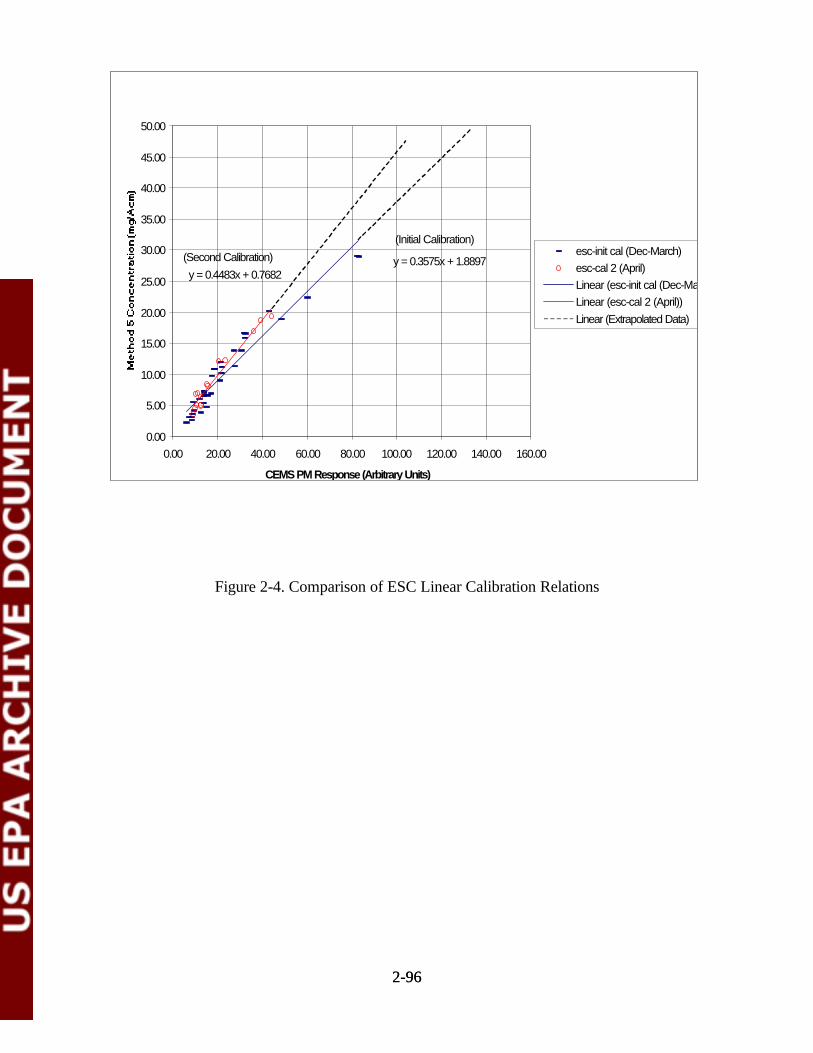
y = 0.3575x + 1.8897y = 0.4483x + 0.7682

0.00

5.00

10.00

15.00

20.00

25.00

30.00

35.00

40.00

45.00

50.00

0.00 20.00 40.00 60.00 80.00 100.00 120.00 140.00 160.00

CEMS PM Response (Arbitrary Units)

esc-init cal (Dec-March)esc-cal 2 (April)Linear (esc-init cal (Dec-March))Linear (esc-cal 2 (April))Linear (Extrapolated Data)

(Initial Calibration)(Second Calibration)

2-962-96

Figure 2-4. Comparison of ESC Linear Calibration Relations

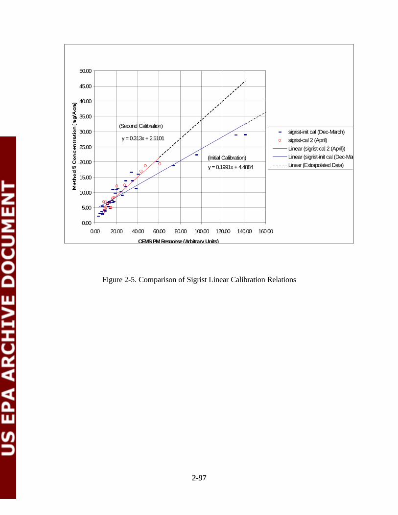
y = 0.313x + 2.5101

y = 0.1991x + 4.4884

0.00

5.00

10.00

15.00

20.00

25.00

30.00

35.00

40.00

45.00

50.00

0.00 20.00 40.00 60.00 80.00 100.00 120.00 140.00 160.00

CEMS PM Response (Arbitrary Units)

sigrist-init cal (Dec-March)sigrist-cal 2 (April)Linear (sigrist-cal 2 (April))Linear (sigrist-init cal (Dec-March))Linear (Extrapolated Data)

(Initial Calibration)

(Second Calibration)

2-972-97

Figure 2-5. Comparison of Sigrist Linear Calibration Relations

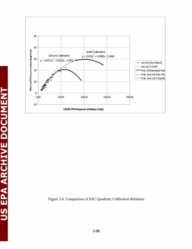
y = -0.003x2 + 0.6086x - 1.3406

y = -0.0071x2 + 0.8132x - 2.6952

-10

0

10

20

30

40

50

0.00 50.00 100.00 150.00 200.00

CEMS PM Response (Arbitrary Units)

esc-init (Dec-March)esc-cal 2 (April)Poly. (Extrapolated Data)Poly. (esc-init (Dec-March))Poly. (esc-cal 2 (April))

(Second Calibration)(Initial Calibration)

2-982-98

Figure 2-6. Comparison of ESC Quadratic Calibration Relations

y = -0.0014x2 + 0.3825x + 1.7373

y = -0.0035x2 + 0.5363x + 0.171

-10.00

0.00

10.00

20.00

30.00

40.00

50.00

0.00 50.00 100.00 150.00 200.00

CEMS PM Response (Arbitrary Units)

sigrist-init cal (Dec-March)sigrist-cal 2 (April)Poly. (sigrist-init cal (Dec-March))Poly. (Extrapolated Data)Poly. (sigrist-cal 2 (April))

(Initial Calibration)

(Second Caliobration)

2-992-99

Figure 2-7. Comparison of Sigrist Quadratic Calibration Relations

-10.00

0.00

10.00

20.00

30.00

40.00

50.00

0.00 20.00 40.00 60.00 80.00 100.00 120.00 140.00 160.00

CEMS PM Response (Arbitrary Units)

esc-init (Dec-March)y_pred +/- con intLogrithmic y_predy_pred +/- tol int

y = 23.765 Log (x) - 19.977

2-1002-100

Figure 2-8. Statistical Evaluation of ESC Logarithmic Relation for Initial Calibration

-10.00

0.00

10.00

20.00

30.00

40.00

50.00

0.00 20.00 40.00 60.00 80.00 100.00 120.00 140.00 160.00

CEMS PM Response (Arbitrary Units)

esc-cal 2 (April)y_pred +/- con intLogrithmic y_predy_pred +/- tol int

y = 22.854 Log (x) - 18.501

2-1012-101

Figure 2-9. Statistical Evaluation of ESC Logarithmic Relation for Second Calibration

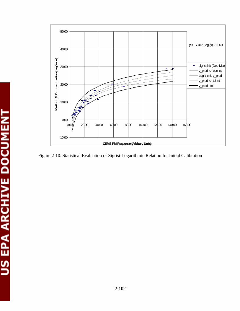
-10.00

0.00

10.00

20.00

30.00

40.00

50.00

0.00 20.00 40.00 60.00 80.00 100.00 120.00 140.00 160.00

CEMS PM Response (Arbitrary Units)

sigrist-init (Dec-March)y_pred +/- con intLogrithmic y_predy_pred +/- tol inty_pred - tol

y = 17.042 Log (x) - 11.608

2-1022-102

Figure 2-10. Statistical Evaluation of Sigrist Logarithmic Relation for Initial Calibration

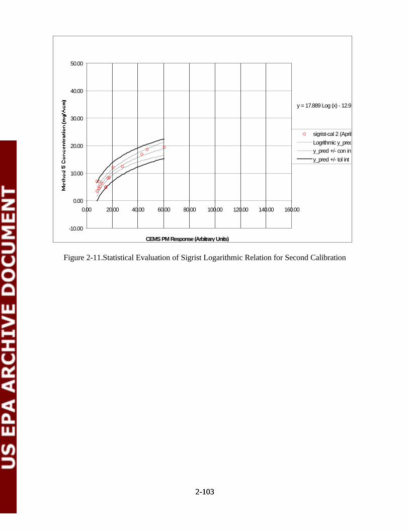
-10.00

0.00

10.00

20.00

30.00

40.00

50.00

0.00 20.00 40.00 60.00 80.00 100.00 120.00 140.00 160.00

CEMS PM Response (Arbitrary Units)

sigrist-cal 2 (April)Logrithmic y_predy_pred +/- con inty_pred +/- tol int

y = 17.889 Log (x) - 12.932

2-1032-103

Figure 2-11.Statistical Evaluation of Sigrist Logarithmic Relation for Second Calibration

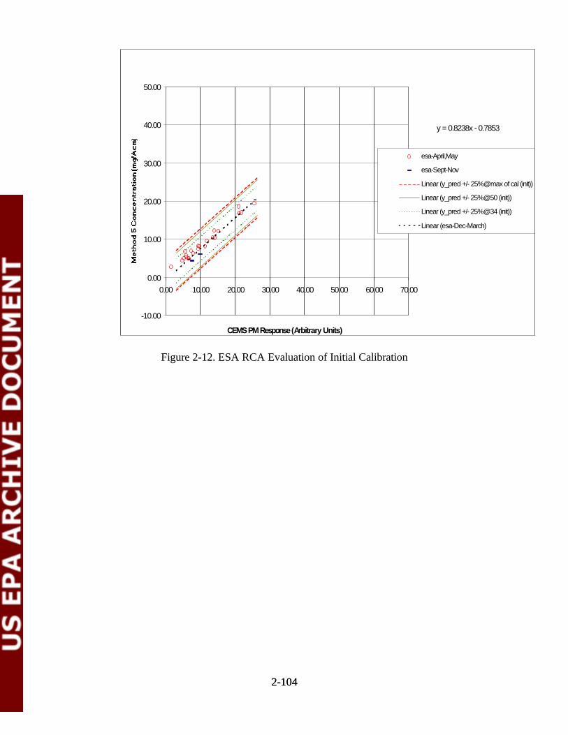
y = 0.8238x - 0.7853

-10.00

0.00

10.00

20.00

30.00

40.00

50.00

0.00 10.00 20.00 30.00 40.00 50.00 60.00 70.00

CEMS PM Response (Arbitrary Units)

esa-April,May

esa-Sept-Nov

Linear (y_pred +/- 25%@max of cal (init))

Linear (y_pred +/- 25%@50 (init))

Linear (y_pred +/- 25%@34 (init))

Linear (esa-Dec-March)

2-1042-104

Figure 2-12. ESA RCA Evaluation of Initial Calibration

y = 0.7662x + 0.9615

-10.00

0.00

10.00

20.00

30.00

40.00

50.00

0.00 10.00 20.00 30.00 40.00 50.00 60.00 70.00

CEMS PM Response (Arbitrary Units)

esa-Dec,Jan,Feb,March,May

esa-Sept-Nov

Linear (y_pred +/- 25%@max of cal (cal 2))

Linear (y_pred +/- 25%@50 (cal 2))

Linear (y_pred +/- 25%@34 (cal 2))

Linear (esa-April)

2-1052-105

Figure 2-13. ESA RCA Evaluation of Second Calibration

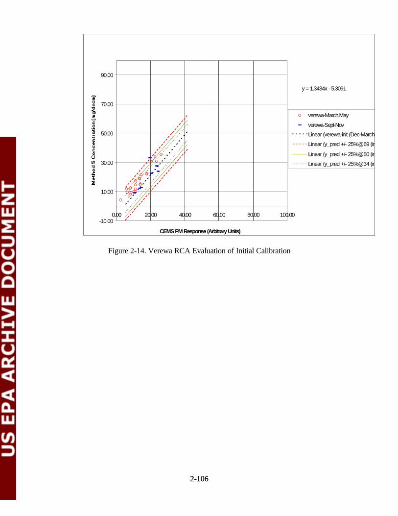
y = 1.3434x - 5.3091

-10.00

10.00

30.00

50.00

70.00

90.00

0.00 20.00 40.00 60.00 80.00 100.00

CEMS PM Response (Arbitrary Units)

verewa-March,May

verewa-Sept-Nov

Linear (verewa-init (Dec-March))

Linear (y_pred +/- 25%@69 (init))

Linear (y_pred +/- 25%@50 (init))

Linear (y_pred +/- 25%@34 (init))

2-1062-106

Figure 2-14. Verewa RCA Evaluation of Initial Calibration

y = 1.4301x - 2.5923

-10.00

10.00

30.00

50.00

70.00

90.00

0.00 20.00 40.00 60.00 80.00 100.00

CEMS PM Response (Arbitrary Units)

verewa-Dec,Jan,Feb,March,May

verewa-Sept-Nov

Linear (verewa-cal 2 (April))

Linear (y_pred +/- 25%@max of cal (cal 2))

Linear (y_pred +/- 25%@50 (cal 2))

Linear (y_pred +/- 25%@34 (cal 2))

2-1072-107

Figure 2-15. Verewa RCA Evaluation of Second Calibration

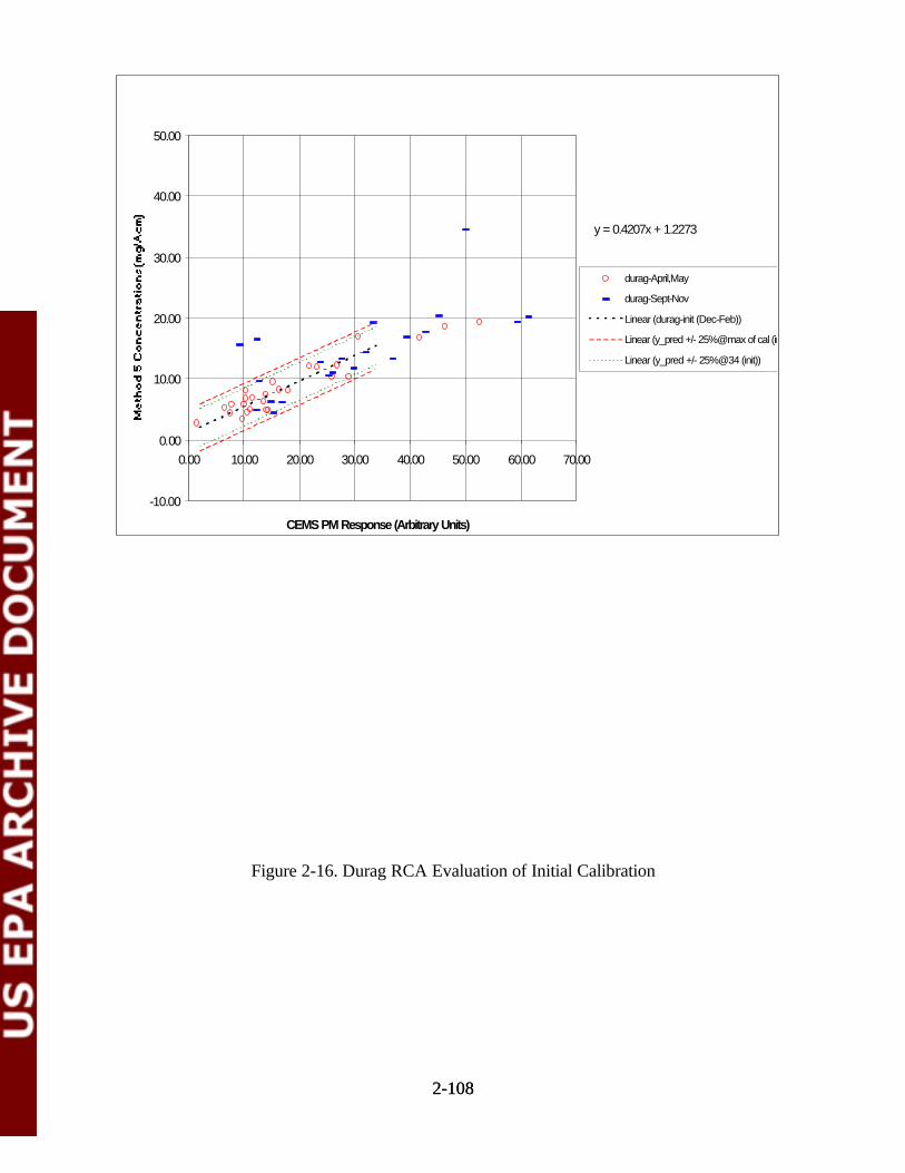
y = 0.4207x + 1.2273

-10.00

0.00

10.00

20.00

30.00

40.00

50.00

0.00 10.00 20.00 30.00 40.00 50.00 60.00 70.00

CEMS PM Response (Arbitrary Units)

durag-April,May

durag-Sept-Nov

Linear (durag-init (Dec-Feb))

Linear (y_pred +/- 25%@max of cal (init))

Linear (y_pred +/- 25%@34 (init))

2-1082-108

Figure 2-16. Durag RCA Evaluation of Initial Calibration

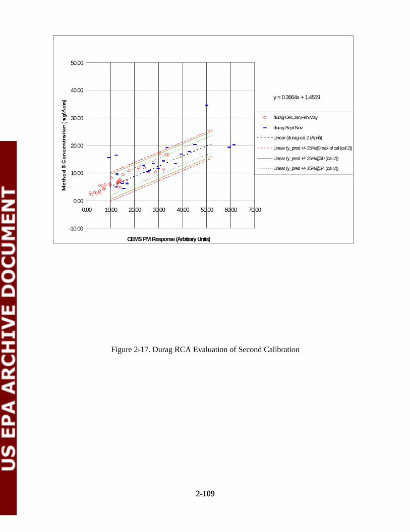
y = 0.3664x + 1.4559

-10.00

0.00

10.00

20.00

30.00

40.00

50.00

0.00 10.00 20.00 30.00 40.00 50.00 60.00 70.00

CEMS PM Response (Arbitrary Units)

durag-Dec,Jan,Feb,May

durag-Sept-Nov

Linear (durag-cal 2 (April))

Linear (y_pred +/- 25%@max of cal (cal 2))

Linear (y_pred +/- 25%@50 (cal 2))

Linear (y_pred +/- 25%@34 (cal 2))

2-1092-109

Figure 2-17. Durag RCA Evaluation of Second Calibration

y = 23.765x - 19.977

-10.00

0.00

10.00

20.00

30.00

40.00

50.00

0.00 0.50 1.00 1.50 2.00 2.50

Log ( CEMS PM Response )

esc-April,May

esc-Sept-Nov

Linear (esc-init cal (Dec-March))

Linear (y_pred +/- 25%@max of cal (init))

Linear (y_pred +/- 25%@50 (init))

Linear (y_pred +/- 25%@34 (init))

2-1102-110

Figure 2-18. ESC RCA Evaluation of Initial Calibration

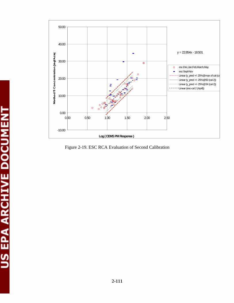
y = 22.854x - 18.501

-10.00

0.00

10.00

20.00

30.00

40.00

50.00

0.00 0.50 1.00 1.50 2.00 2.50

Log ( CEMS PM Response )

esc-Dec,Jan,Feb,March,May

esc-Sept-NovLinear (y_pred +/- 25%@max of cal (cal 2))

Linear (y_pred +/- 25%@50 (cal 2))

Linear (y_pred +/- 25%@34 (cal 2))Linear (esc-cal 2 (April))

2-1112-111

Figure 2-19. ESC RCA Evaluation of Second Calibration

y = 17.042x - 11.608

-10.00

0.00

10.00

20.00

30.00

40.00

50.00

0.00 0.50 1.00 1.50 2.00 2.50

Log ( CEMS PM Response )

sigrist-April,May

sigrist-Sept-Nov

Linear (sigrist-init (Dec-March))

Linear (y_pred +/- 25%@max of cal (init))

Linear (y_pred +/- 25%@50 (init))

Linear (y_pred +/- 25%@34 (init))

2-1122-112

Figure 2-20. Sigrist RCA Evaluation of Initial Calibration

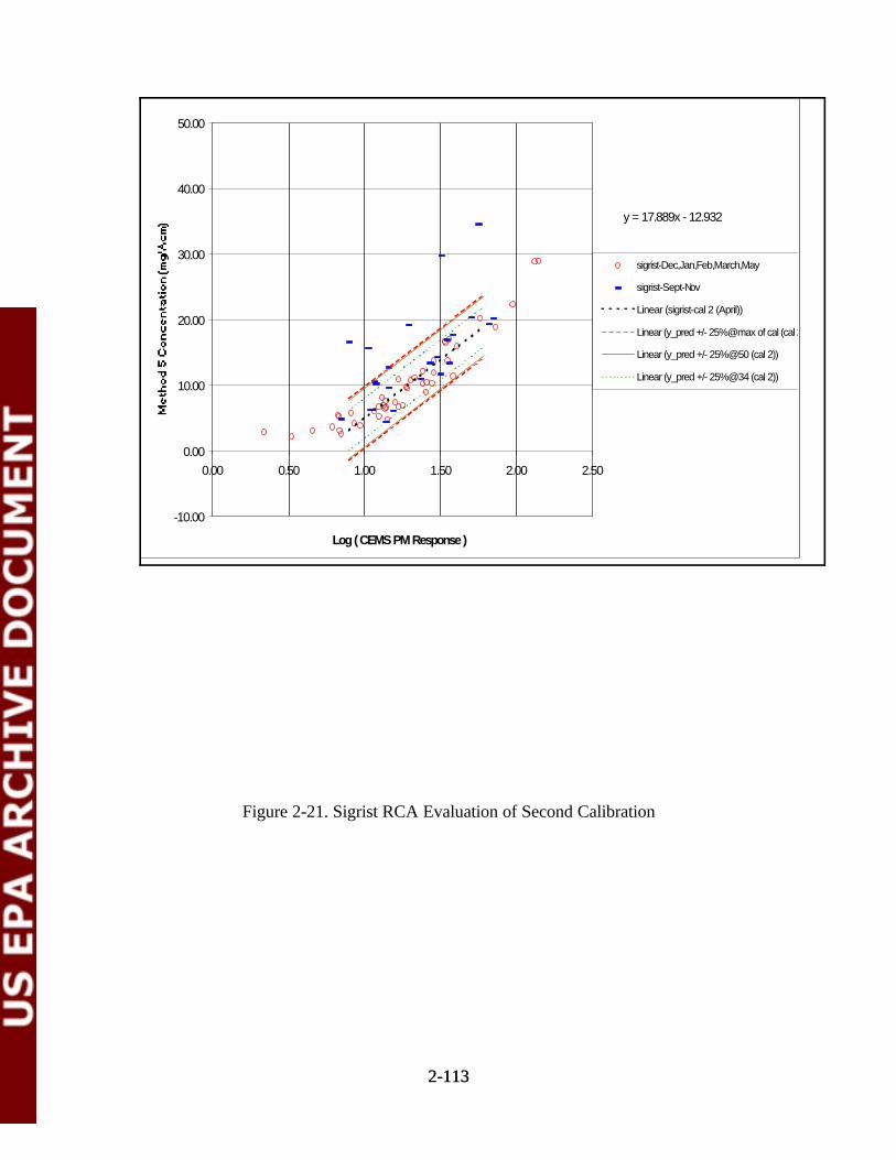
Figure 2-21. Sigrist RCA Evaluation of Second Calibration

y = 17.889x - 12.932

-10.00

0.00

10.00

20.00

30.00

40.00

50.00

0.00 0.50 1.00 1.50 2.00 2.50

Log ( CEMS PM Response )

sigrist-Dec,Jan,Feb,March,May

sigrist-Sept-Nov

Linear (sigrist-cal 2 (April))

Linear (y_pred +/- 25%@max of cal (cal 2))

Linear (y_pred +/- 25%@50 (cal 2))

Linear (y_pred +/- 25%@34 (cal 2))

2-1132-113

Figure 2-21. Sigrist RCA Evaluation of Second Calibration

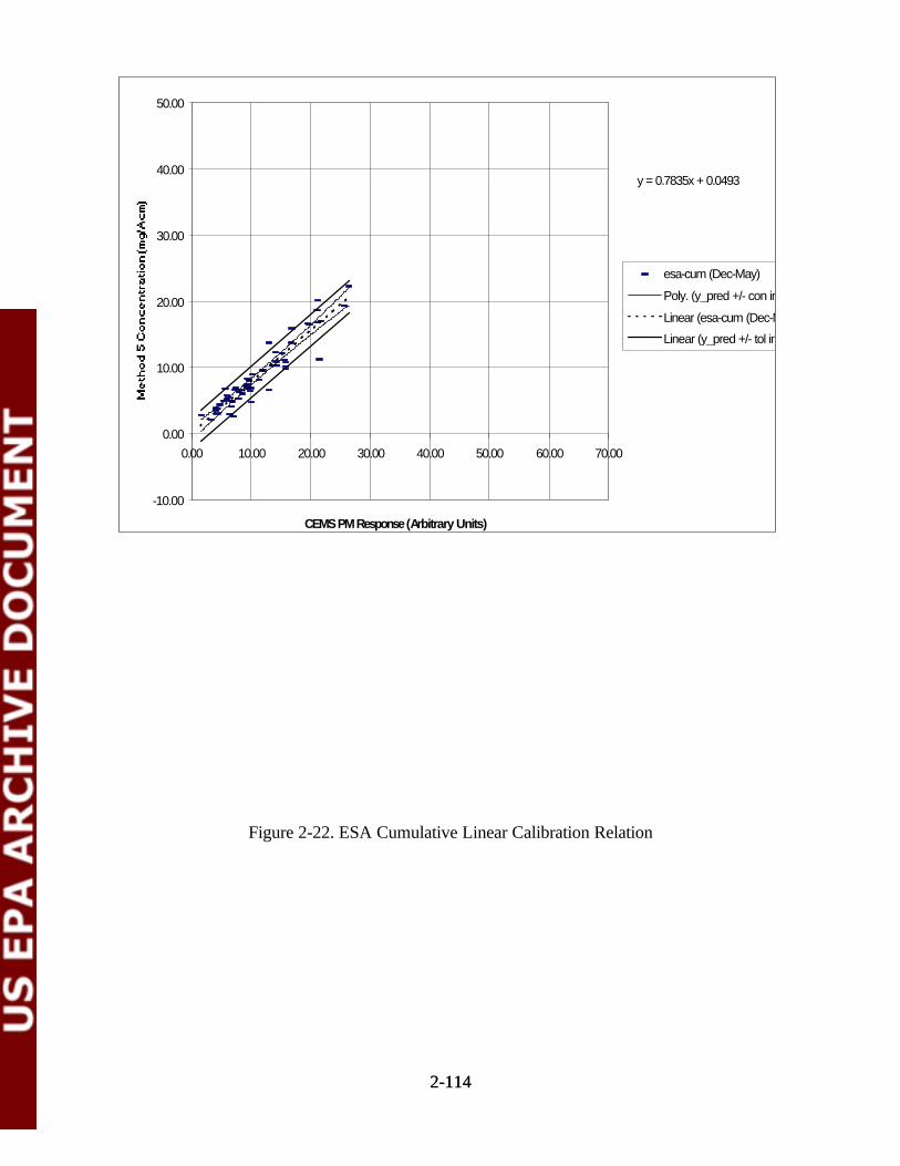
y = 0.7835x + 0.0493

-10.00

0.00

10.00

20.00

30.00

40.00

50.00

0.00 10.00 20.00 30.00 40.00 50.00 60.00 70.00

CEMS PM Response (Arbitrary Units)

esa-cum (Dec-May)

Poly. (y_pred +/- con int)

Linear (esa-cum (Dec-May))

Linear (y_pred +/- tol int)

2-1142-114

Figure 2-22. ESA Cumulative Linear Calibration Relation

y = 1.2646x - 2.0646

-10.00

10.00

30.00

50.00

70.00

90.00

0.00 20.00 40.00 60.00 80.00 100.00

CEMS PM Response (Arbitrary Units)

verewa-cum (Dec-May)

Poly. (y_pred +/- con int)

Linear (verewa-cum (Dec-May))

Linear (y_pred +/- tol int)

2-1152-115

Figure 2-23. Verewa Cumulative Linear Calibration Relation

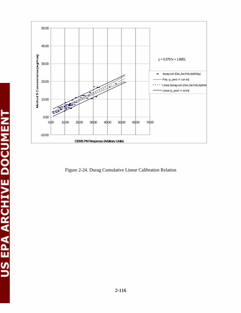
y = 0.3757x + 1.8951

-10.00

0.00

10.00

20.00

30.00

40.00

50.00

0.00 10.00 20.00 30.00 40.00 50.00 60.00 70.00

CEMS PM Response (Arbitrary Units)

durag-cum (Dec,Jan,Feb,April,May)

Poly. (y_pred +/- con int)

Linear (durag-cum (Dec,Jan,Feb,April,May))

Linear (y_pred +/- tol int)

2-1162-116

Figure 2-24. Durag Cumulative Linear Calibration Relation

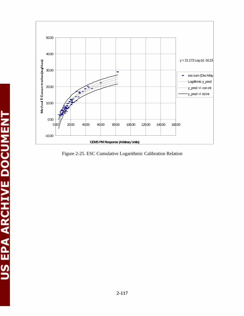
-10.00

0.00

10.00

20.00

30.00

40.00

50.00

0.00 20.00 40.00 60.00 80.00 100.00 120.00 140.00 160.00

CEMS PM Response (Arbitrary Units)

esc-cum (Dec-May)

Logrithmic y_pred

y_pred +/- con int

y_pred +/- tol int

y = 21.173 Log (x) -16.234

2-1172-117

Figure 2-25. ESC Cumulative Logarithmic Calibration Relation

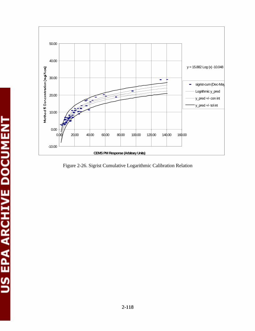
-10.00

0.00

10.00

20.00

30.00

40.00

50.00

0.00 20.00 40.00 60.00 80.00 100.00 120.00 140.00 160.00

CEMS PM Response (Arbitrary Units)

sigrist-cum (Dec-May)

Logrithmic y_pred

y_pred +/- con int

y_pred +/- tol int

y = 15.882 Log (x) -10.048

2-1182-118

Figure 2-26. Sigrist Cumulative Logarithmic Calibration Relation

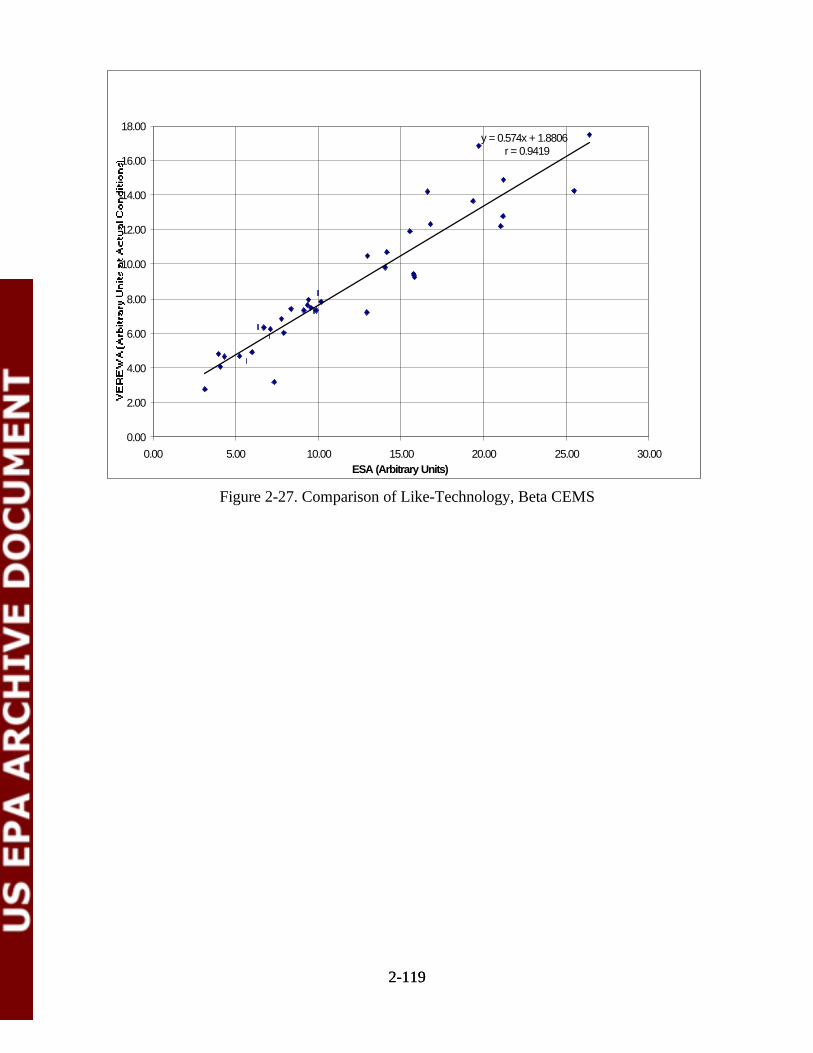
y = 0.574x + 1.8806

0.00

2.00

4.00

6.00

8.00

10.00

12.00

14.00

16.00

18.00

0.00 5.00 10.00 15.00 20.00 25.00 30.00ESA (Arbitrary Units)

r = 0.9419

2-1192-119

Figure 2-27. Comparison of Like-Technology, Beta CEMS

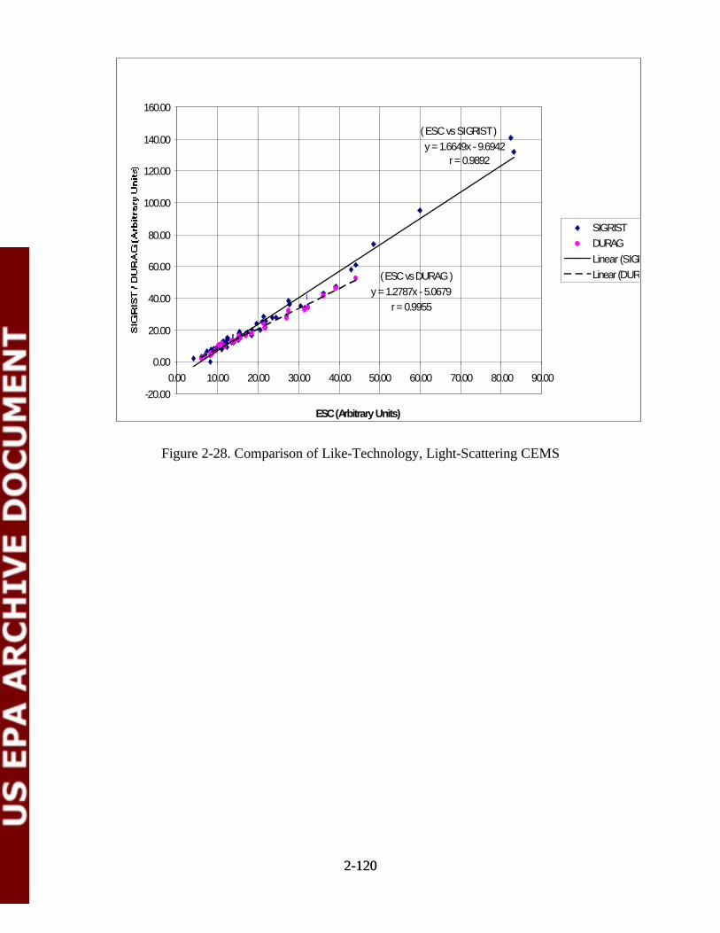
y = 1.6649x - 9.6942

y = 1.2787x - 5.0679

-20.00

0.00

20.00

40.00

60.00

80.00

100.00

120.00

140.00

160.00

0.00 10.00 20.00 30.00 40.00 50.00 60.00 70.00 80.00 90.00

ESC (Arbitrary Units)

SIGRISTDURAGLinear (SIGRIST)Linear (DURAG)

r = 0.9892

r = 0.9955

( ESC vs SIGRIST )

( ESC vs DURAG )

2-1202-120

Figure 2-28. Comparison of Like-Technology, Light-Scattering CEMS

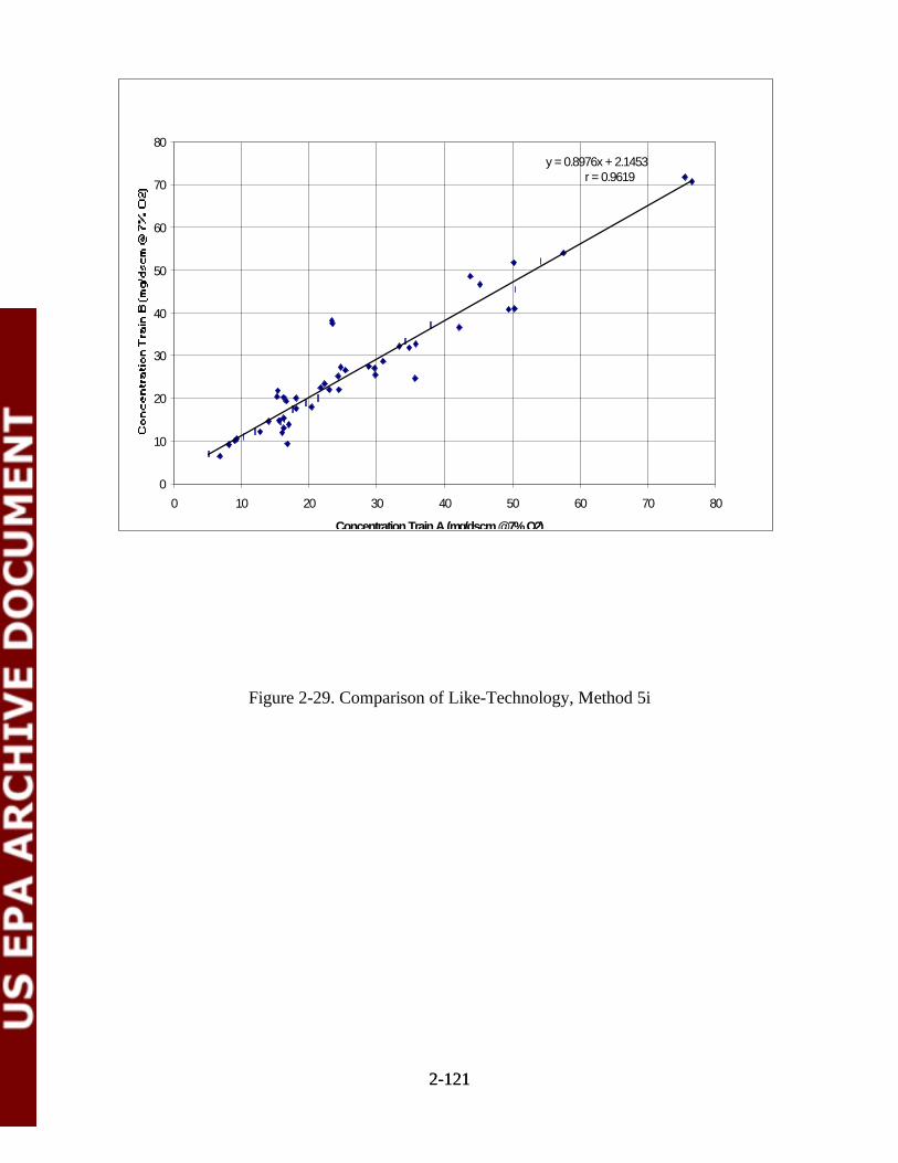
y = 0.8976x + 2.1453

0

10

20

30

40

50

60

70

80

0 10 20 30 40 50 60 70 80

Concentration Train A (mg/dscm @7% O2)

r = 0.9619

2-1212-121

Figure 2-29. Comparison of Like-Technology, Method 5i

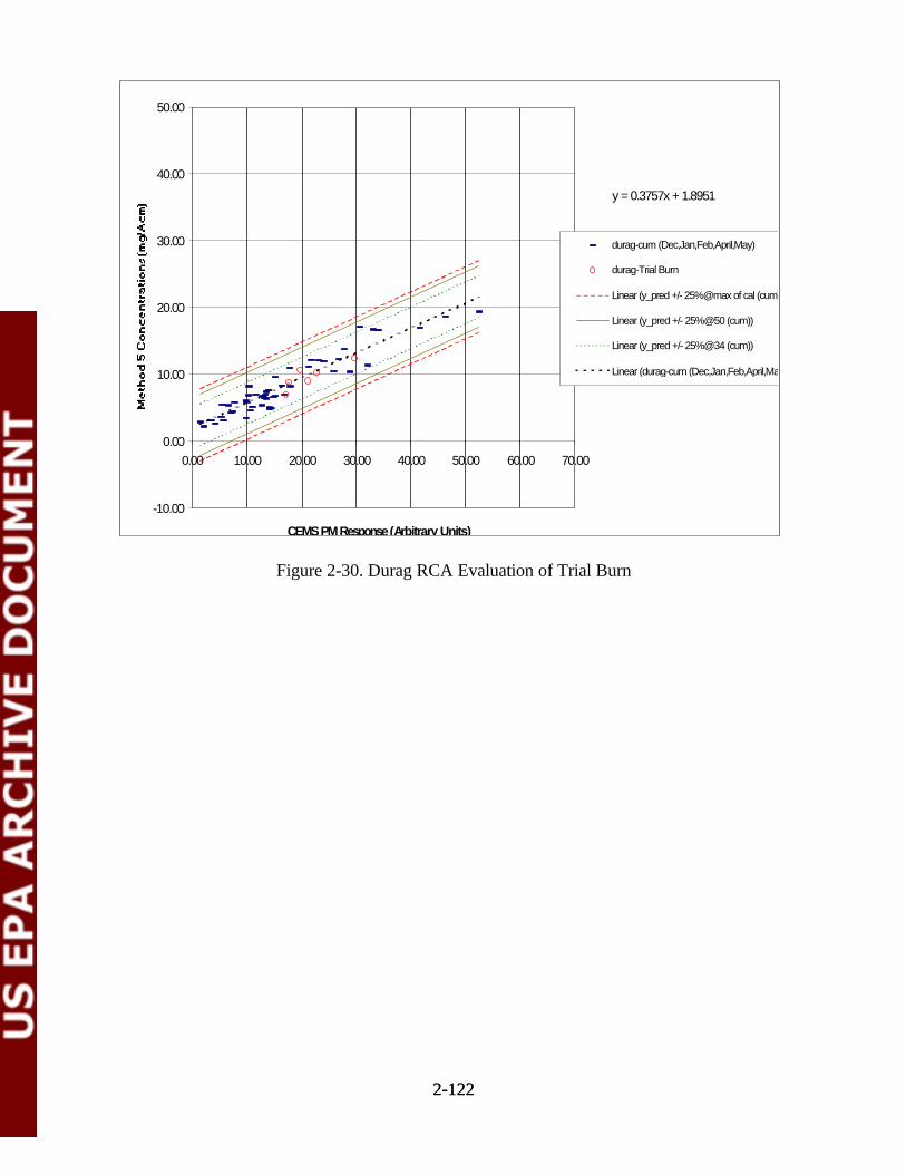
y = 0.3757x + 1.8951

-10.00

0.00

10.00

20.00

30.00

40.00

50.00

0.00 10.00 20.00 30.00 40.00 50.00 60.00 70.00

CEMS PM Response (Arbitrary Units)

durag-cum (Dec,Jan,Feb,April,May)

durag-Trial Burn

Linear (y_pred +/- 25%@max of cal (cum))

Linear (y_pred +/- 25%@50 (cum))

Linear (y_pred +/- 25%@34 (cum))

Linear (durag-cum (Dec,Jan,Feb,April,May))

2-1222-122

Figure 2-30. Durag RCA Evaluation of Trial Burn

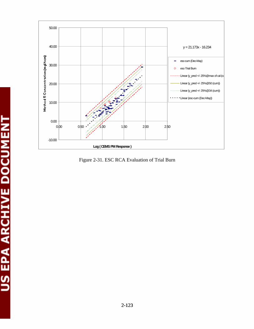
y = 21.173x - 16.234

-10.00

0.00

10.00

20.00

30.00

40.00

50.00

0.00 0.50 1.00 1.50 2.00 2.50

Log ( CEMS PM Response )

esc-cum (Dec-May)

esc-Trial Burn

Linear (y_pred +/- 25%@max of cal (cum))

Linear (y_pred +/- 25%@50 (cum))

Linear (y_pred +/- 25%@34 (cum))

Linear (esc-cum (Dec-May))

2-1232-123

Figure 2-31. ESC RCA Evaluation of Trial Burn

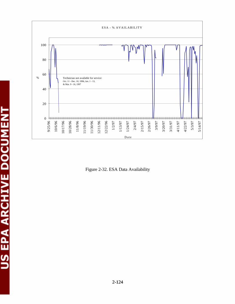
ESA - % AVAILABILITY

0

20

40

60

80

1009/

25/9

6

10/6

/96

10/1

7/96

10/2

8/96

11/8

/96

11/1

9/96

11/3

0/96

12/1

1/96

12/2

2/96

1/2/

97

1/13

/97

1/24

/97

2/4/

97

2/15

/97

2/26

/97

3/9/

97

3/20

/97

3/31

/97

4/11

/97

4/22

/97

5/3/

97

5/14

/97

Date

% Technician not available for service:Oct. 11 - Dec. 10, 1996, Jan. 1 - 13,& Mar. 9 - 16, 1997

2-1242-124

Figure 2-32. ESA Data Availability

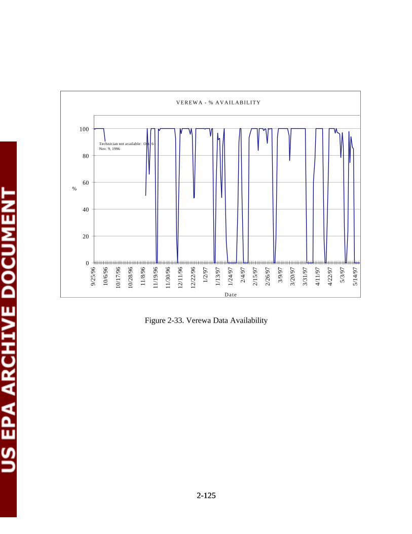
VEREWA - % AVAILABILITY

0

20

40

60

80

100

9/25

/96

10/6

/96

10/1

7/96

10/2

8/96

11/8

/96

11/1

9/96

11/3

0/96

12/1

1/96

12/2

2/96

1/2/

97

1/13

/97

1/24

/97

2/4/

97

2/15

/97

2/26

/97

3/9/

97

3/20

/97

3/31

/97

4/11

/97

4/22

/97

5/3/

97

5/14

/97

Date

%

Technician not available: Oct. 6 - Nov. 9, 1996

2-1252-125

Figure 2-33. Verewa Data Availability

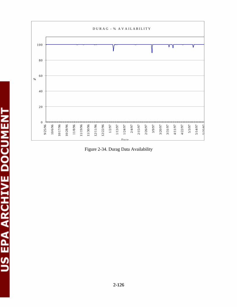
D U R A G - % A V A I L A B I L I T Y

0

20

40

60

80

1009/

25/9

6

10/6

/96

10/1

7/96

10/2

8/96

11/8

/96

11/1

9/96

11/3

0/96

12/1

1/96

12/2

2/96

1/2/

97

1/13

/97

1/24

/97

2/4/

97

2/15

/97

2/26

/97

3/9/

97

3/20

/97

3/31

/97

4/11

/97

4/22

/97

5/3/

97

5/14

/97

5/25

/97

D a t e

%

2-1262-126

Figure 2-34. Durag Data Availability

ESC - % AVAILABILITY

0

20

40

60

80

1009/

25/9

6

10/5

/96

10/1

5/96

10/2

5/96

11/4

/96

11/1

4/96

11/2

4/96

12/4

/96

12/1

4/96

12/2

4/96

1/3/

97

1/13

/97

1/23

/97

2/2/

97

2/12

/97

2/22

/97

3/4/

97

3/14

/97

3/24

/97

4/3/

97

4/13

/97

4/23

/97

5/3/

97

5/13

/97

Date

%

2-1272-127

Figure 2-35. ESC Data Availability

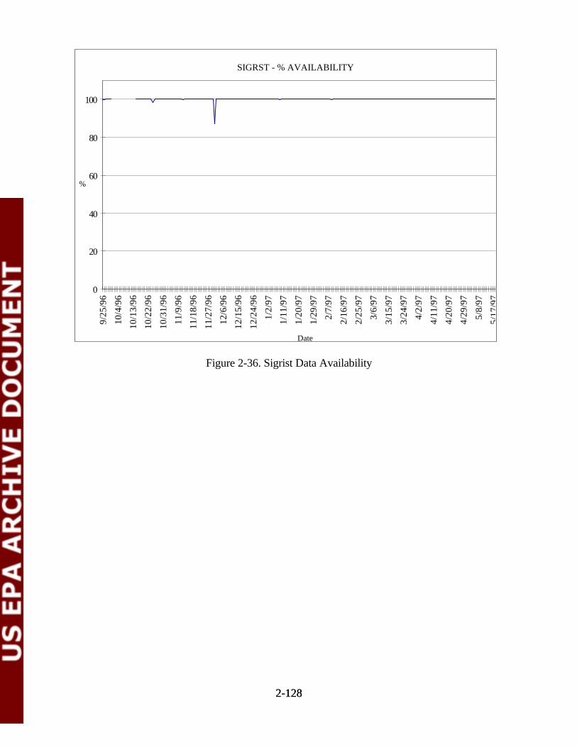
SIGRST - % AVAILABILITY

0

20

40

60

80

1009/

25/9

6

10/4

/96

10/1

3/96

10/2

2/96

10/3

1/96

11/9

/96

11/1

8/96

11/2

7/96

12/6

/96

12/1

5/96

12/2

4/96

1/2/

97

1/11

/97

1/20

/97

1/29

/97

2/7/

97

2/16

/97

2/25

/97

3/6/

97

3/15

/97

3/24

/97

4/2/

97

4/11

/97

4/20

/97

4/29

/97

5/8/

97

5/17

/97

Date

%

2-1282-128

Figure 2-36. Sigrist Data Availability

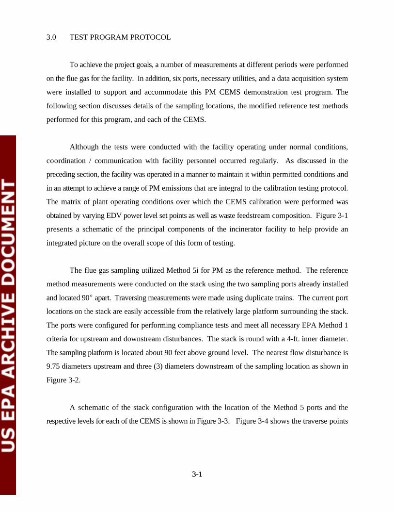
3-13-1

3.0 TEST PROGRAM PROTOCOL

To achieve the project goals, a number of measurements at different periods were performed

on the flue gas for the facility. In addition, six ports, necessary utilities, and a data acquisition system

were installed to support and accommodate this PM CEMS demonstration test program. The

following section discusses details of the sampling locations, the modified reference test methods

performed for this program, and each of the CEMS.

Although the tests were conducted with the facility operating under normal conditions,

coordination / communication with facility personnel occurred regularly. As discussed in the

preceding section, the facility was operated in a manner to maintain it within permitted conditions and

in an attempt to achieve a range of PM emissions that are integral to the calibration testing protocol.

The matrix of plant operating conditions over which the CEMS calibration were performed was

obtained by varying EDV power level set points as well as waste feedstream composition. Figure 3-1

presents a schematic of the principal components of the incinerator facility to help provide an

integrated picture on the overall scope of this form of testing.

The flue gas sampling utilized Method 5i for PM as the reference method. The reference

method measurements were conducted on the stack using the two sampling ports already installed

and located 90 apart. Traversing measurements were made using duplicate trains. The current port

locations on the stack are easily accessible from the relatively large platform surrounding the stack.

The ports were configured for performing compliance tests and meet all necessary EPA Method 1

criteria for upstream and downstream disturbances. The stack is round with a 4-ft. inner diameter.

The sampling platform is located about 90 feet above ground level. The nearest flow disturbance is

9.75 diameters upstream and three (3) diameters downstream of the sampling location as shown in

Figure 3-2.

A schematic of the stack configuration with the location of the Method 5 ports and the

respective levels for each of the CEMS is shown in Figure 3-3. Figure 3-4 shows the traverse points

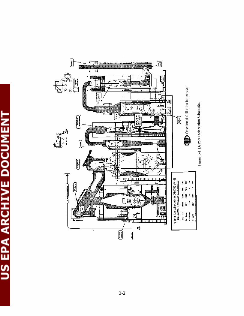
3-23-2

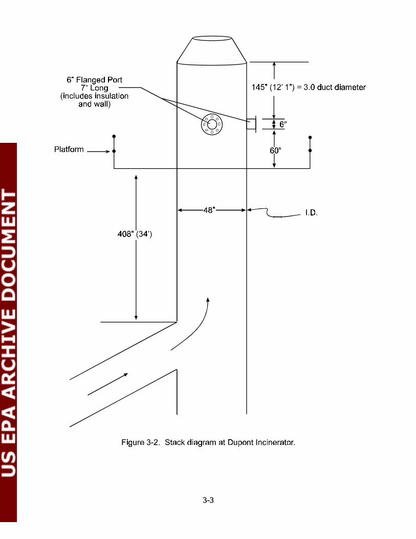
3-33-3

3-43-4

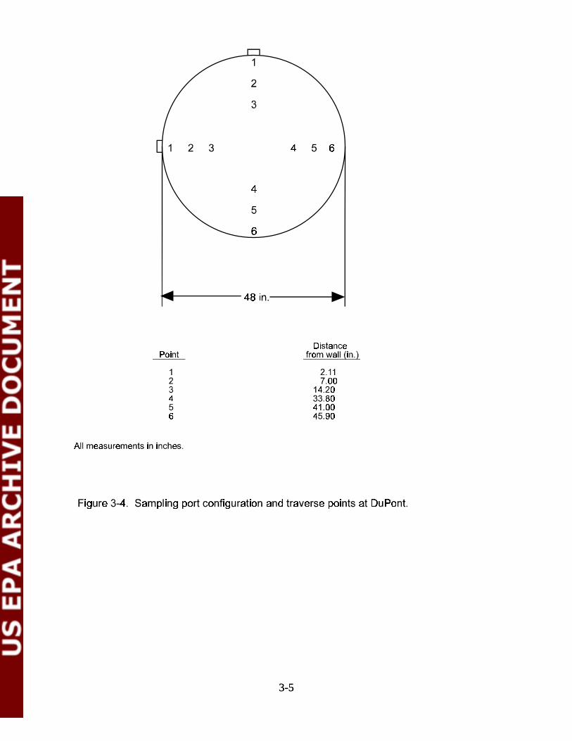
3-53-5

3-63-6

that were used for the Modified Method 5 measurements. The port lengths and actual stack were

measured on-site, and the appropriate adjustments to the traverse points were measured on-site, and

the appropriate adjustments to the traverse points were implemented. For the course of the program,

the flue gas conditions at this sampling location showed variations in the following ranges:

Temperature: 285 - 325 F (with steam reheat)

Static pressure: +0.2 inches of water

Flow Rate: 13,000 - 15,000 dscfm

Velocity: 10 - 12 m/sec

Moisture: 16 - 30 %

PM Loading: 5 - 100 mg/dscm at 7% O2

3.1 Reference Method and CEMS Sampling Locations

The reference method measurements with the traversing trains were made using two pre-

existing 90 - opposed ports, while a third port was used for the single point reference method0

sampling in the initial testing phase. The CEMS were located on the stack platform at ports

specially installed for each CEMS. The CEMS ports were located around the stack at various,

nearby levels (within 3 feet) above the plane of the reference method location. They were

arranged around the stack such that no CEMS samples are directly downstream of another CEMS

or the reference method trains. Figures 3-5 and 3-6 are helpful in illustrating the staggered

arrangements of the sampling port locations for the reference methods and the CEMS.

3.2 Reference Method Sampling Procedures

To achieve acceptable data from this test program, detection limits need to be established and

achieved. For flue gas measurements, the detection limit is a function of the analytical detection limit

and the total sample collected. Depending on PM concentrations, the M5 sampling trains were

3-73-7

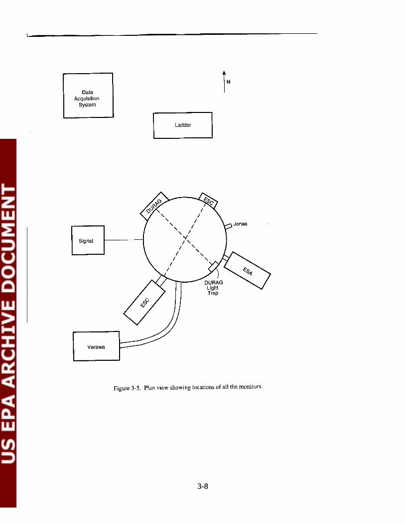
3-83-8

3-93-9

operated for 18 to 72 minutes. Details of the sample trains, sampling procedures, and recovery

procedures follow.

3.2.1 Sample Train Description and Sampling Procedures

EPA Methods 1, 2 - Traverse Point Determination, Stack Gas Temperature, Velocity, and

Volumetric Flow Rate

EPA Method 1 was used to determine the sample and velocity traverse points for velocity

measurements and isokinetic sampling. With EPA Method 1, the duct or stack cross-section is

divided into equal areas. A traverse point is located in the centroid of each of the resulting areas.

The minimum number of equal areas and traverse points depends on the duct diameter and

length in equivalent diameters directly upstream and downstream of the sample location. Schematic

layouts of the sample locations and traverse points are shown in Figure 3-2 and 3-4.

EPA Method 2 was used to determine the stack gas temperature, velocity, and volumetric

flow rate. The velocity of the stack gas was determined from the density of the gas and the

measurement of the average velocity head. A stainless steel sheathed Type-K thermocouple (TC)

was used to measure stack temperature, while a stainless steel Type-S pitot, and an inclined

manometer is used to measure stack gas velocity. To minimize mutual interference, the TC and pitot

are assembled according to the method specifications. Pre-test and post-test leak checks were

conducted to ensure the accuracy of the velocity measurements.

EPA Methods 3A and 4 - Stack Gas Analysis and Moisture Content Determination

EPA Method 3 was used to determine the stack gas oxygen (O ) and carbon dioxide (CO )2 2

concentrations and the dry molecular weight. An integrated stack gas sample was collected from the

M5 sample train and examined using an Fyrite analyzer to determine carbon dioxide and oxygen

content. The dry molecular weight of the stack gas was calculated using the measured O and CO2 2

levels, assuming the remainder of the stack gas composition is nitrogen. Low levels (ppm range) of

3-103-10

CO, SO , NO , hydrocarbons, and other compounds are not significant factors in the molecular2 x

weight determination. The molecular weight and excess O levels are used in velocity, isokinetic2

sampling rate, and pollutant emission concentration calculations.

EPA Method 4 was used to determine the moisture content of the stack gas for a pre-test

determination. Moisture was determined from all M5 sampling trains during the calibration tests.

EPA Method 5 - Determination of Particulate Emissions from Stationary Sources

As directed by the Code of Federal Regulations, Method 5 applies specifically to the

gravimetric determination of the emission rate of particulate matter (PM) from stationary sources.

For this to be achieved, the location of the sampling points must be determined (Method 1) and the

volumetric flow rate (Method 2) calculated. To calculate the volumetric flow rate, the values for

carbon dioxide and oxygen contents (Method 3), and moisture content (Method 4) must be

determined, per the methods discussed in the previous section.

With EPA Method 5, a gas sample is withdrawn isokinetically from the stationary source and

passed through a heated glass fiber filter. The filter collects any solid PM contained in the effluent

gas stream while allowing any uncombined water vapor to pass through for collection in the impinger

train containing a known volume of water. The mass of the particulate is then determined by

desiccating the filter and associated probe rinse. For this study, the recovery of the filter was

modified to accommodate a new light-weight filter housing. The housing is designed such that the

filter and the front half of the filter housing make one integral piece that can be tared as a single unit.

The moisture content was determined by measuring the amount of water collected in the impingers.

The volumetric flow rate of the gas stream was determined by the velocity and temperature traverse.

These values were then used to calculate the particulate mass concentration. Figure 3-7 gives a

schematic of the modified Method 5 sampling train.

3-113-11

3-123-12

The largest area of significant error in Method 5 testing at low PM concentrations comes from

inaccuracies produced by unnecessary filter handling after pre-weighing and before final weighing.

In the original Method 5 procedure, 1) filters were pre-weighed and then handled during assembly

into the filter holder; 2) following sampling, filters were handled during recovery from the filter

assembly, desiccated, and then weighed. As a result of this procedure, it was common for small filter

pieces/fibers to be inadvertently removed/lost (after pre-taring) during filter handling in assembly

and/or in recovery (before final weighing). The problem with this approach stems from filter handling

after pre-weighing; it was further compounded by further handling before final weighing.

For this PM CEMS program the standard Method 5 filter and its holding assembly were

replaced with a smaller (47 mm) filter and smaller holder to minimize inadvertent loss of small filter

pieces in its handling during assembly and recovery. The new filter holder allows the filter to be

assembled, and then pre-weighed in the low-weight assembly; following sampling, the assembly was

desiccated and then weighed before disassembly -- without the filter being directly handled during

pre-test and post-test activities. This approach eliminates filter handling after pre-weighing and

before final weighing and, thereby, simplifies as well as improves the method.

The filter assemblies were uniquely marked with stamped, metal tags and tared, and the filters

used for sampling were immediately removed and carefully transferred to a desiccator. After allowing

the filter to cool and following a successful post-test leak check, the filter holder was removed from

the sample oven box and the exposed ends of the probe and filter holder were immediately covered

with Teflon tape. The filter holder was taken to the recovery area; the probe and impingers were

immediately recovered on the stack platform. The filter was recovered by loosening the rings of the

holder and separating the filter halves. The front half of the filter housing and the filter disassemble

as one unit and were placed directly into a desiccator to continue cooling and allow the weight to

stabilize. The average weight of these units was approximately 30 grams, allowing the pre-taring and

final weighings to be performed on a micro-balance with a resolution of ±0.1 mg.

To determine stack gas moisture concentrations, each of the four impingers were individually

weighed to the nearest 0.5g before and after sampling.

3-133-13

Sample train front half recovery was accomplished using a damp cloth or paper towel to

remove any accumulated particulate from the exteriors of the nozzle and the probe. Then, the probe

and nozzle were rinsed three times using acetone and a small brush. The rinsate was placed in a small

pre-cleaned sample jar labeled with a unique sample log number including the run and sample train

number.

Analysis of the samples for particulate catch was accomplished using a micro-balance with

a resolution to 0.1 mg resolution. The filter and front half rinse were weighed after being desiccated

for several hours. The acetone rinses were transferred into Teflon or glass beakers and then

evaporated, desiccated and weighed separately. The samples were evaporated at 20° ± 6°C (68° ±

10°F). The samples were weighed until three successive weighings that agreed to ± 0.5 mg for

the filters and ± 1.0 mg for the probe rinses were achieved. Anti-static provisions were used to

minimize fluctuation in weighings. Prior to analysis the balance was calibrated using Class S

weights that are traceable to a National Institute of Standards and Technology (NIST) standard.

3.2.2 Calibration Procedures

All equipment used in this test program was maintained and calibrated using approved

procedures and EPA, American Standards Testing Material (ASTM), and/or National Institute of

Standards and Technology (NIST) traceable reference equipment, where applicable. Calibrations

were routinely performed on all key equipment so that required pre-test calibrations were performed

prior to mobilization. During equipment preparation, the calibration records were reviewed to ensure

that specified calibrations were up-to-date. The applicable equipment was also checked in the field

to assure that handling and use did not affect the calibrations. Following each monthly test series,

the equipment was again routinely calibrated in order to verify continuous calibration status

throughout the on-site testing. If at any time during testing the operator has reason to believe a piece

of equipment may no longer be in calibration due to unusual change in readings or possible damage,

a recalibration was performed to verify accuracy. Equipment which required calibration included

meter boxes, thermocouples, nozzles, and pitot tubes. Reference calibration procedures were

followed when available, and the results properly documented and retained in a calibration log book.

A discussion of the techniques used to calibrate this equipment is presented below.

3-143-14

Type-S Pitot Tube Calibration

The EPA has specified guidelines concerning the construction and geometry of an acceptable

Type-S pitot tube. If the specified design and construction guidelines are met, a pitot tube coefficient

of 0.84 can be used. Information related to the design and construction of the Type-S pitot tube is

presented in detail in Section 3.1.1 of EPA Document 700/4-77/027b. Only Type-S pitot tubes

meeting the required EPA specifications were used during this project. Pitot tubes were inspected

and documented as meeting EPA specifications prior to the field sampling.

Sampling Nozzle Calibration

EPA Method 5 prescribes the use of stainless steel buttonhook nozzles for isokinetic

particulate sampling. However, for this study glass nozzles were used. Calculation of the isokinetic

sampling rate requires that the cross-sectional area of sampling nozzle be accurately and precisely

known. All nozzles used for Methods 5 sampling were thoroughly cleaned, visually inspected, and

calibrated according to the procedure outlined in Section 3.4.2 of EPA Document 600/4-77-027b.

Temperature Measuring Device Calibration

Accurate temperature measurements are required during emission sampling. Bimetallic stem

thermometers and thermocouple temperature sensors were calibrated using the procedure described

in Section 3.4.2 of EPA Document 600/4-77-027b. Each temperature sensor was calibrated at a

minimum of three points above the anticipated range of use against an NIST-traceable mercury-in-

glass thermometer. All sensors were calibrated prior to field sampling.

Dry Gas Meter Calibration

Dry gas meters (DGMs) were used in the Method 5 trains to monitor the sampling gas flow

rate and to measure the sample gas volume. All dry gas meters were calibrated (documented

correction factor) just prior to the departure of the equipment to the field. A post-test calibration

3-153-15

check was performed as soon as possible after the equipment was returned to EER's shop. Pre- and

post-test calibrations agreed within 5%.

Dry gas meters were calibrated using the calibration system. Prior to calibration, a positive

pressure leak-check of the system was performed, using the procedure outlined in Sections 3.3.2 of

EPA Document 600/4-77-27b. The system was placed under approximately 10 inches of water

pressure, and a gauge oil manometer was used to determine if a pressure decrease can be detected

for a one-minute period. If leaks were detected, they were eliminated before actual calibrations were

performed.

After the sampling console was assembled and leak-checked, the pump was allowed to run

for 15 minutes, allowing the pump and dry gas meter to warm up. The valve was then adjusted to

obtain the desired flow rate. For the pre-test calibrations, data were collected at orifice manometer

settings ( H) of 0.5, 1.0, 1.5, 2.0, 3.0, and 4.0 inches of H O. Gas volumes of 5 ft were used for23

the two lower orifice settings and volumes of 10 ft for the higher settings. The individual gas meter3

correction factors (Y) were calculated for each orifice setting and averaged. The method requiresi

that each of the individual correction factors must fall within 2% of the average correction factor or

the meter must be cleaned, adjusted, and recalibrated. For the post-test calibration, the meter was

calibrated three times at the average orifice setting and highest vacuum used during the actual test.

Analytical Balance Calibration

Analytical balances were calibrated over the expected range of use with standard weights

(NIST Class S). Measured values must agree within ± 0.1 mg for the probe rinse and filter weights,

and 1.0 mg for moisture, respectively. The balances were calibrated prior to and during the field

measurement program.

Field checks of balance accuracy were made daily using a set of quality control weights which

have previously been weighed side-by-side with the NIST-traceable weights.

3-163-16

3.2.3 Data Reduction, Validation, and Reporting

Manual methods operations data were input onto computer spreadsheets each day following

receipt from testing. Results of sample weighings were input onto the computer system as soon as

they were available. Data were reduced and analyzed using hand-held calculator programs, computer

spreadsheets, and other computer programs. The actual equations and nomenclature are shown on

the calculator program data sheets and on the spreadsheets. This feature enabled operator and analyst

to become familiar with the programmed computations, gave separate spot-checking of computed

results by hand, and eliminated the need to show equations separately in the text.

Standardized run data forms were used for each method. All run sheets were reviewed daily

by the Field Manager for evaluation of progress, completeness, and problems. Standardized

computer spreadsheets were used to reduce and analyze field data. At the end of each test day, test

data was input onto these spreadsheets. Lab analytical results were not available at the end of each

test day, however, results were input as they became available. A standard data set, which had been

verified by hand, was used to demonstrate the accuracy of the spreadsheet calculations before the test

program.

For each test condition, the field data was reduced manually at the end of each test. An

isokinetic ratio was then estimated at the end of each condition using an average or typical moisture

value. The estimated moisture value, estimated isokinetic ratio, and all intermediate calculations were

noted on the run sheet. Upon entry into the computer spreadsheet program, both the data and

the program were validated by checking the estimated isokinetic ratio against the manually

determined value.

Spreadsheet calculations for the various runs observed the following guidelines:

1. Isokinetic calculations for each train were conducted using the input run data from

that specific run rather than from the average or other values from previous runs.

Stack gas moisture content was determined using the condensed water measured in

3-173-17

that train; and

2. Stack temperature, velocity, and flow rate values for each sampling train were

determined for each specific sampling run.

The accepted range for the isokinetic rate is 90 to 110%. All valid data had isokinetic rates were

within the acceptable range.

Upon daily completion of testing, the Field Manager was responsible for preparation of a data

summary which included:

• Raw data sheets;

• Calculation of isokinetic ratio for each run;

• Traverse start and stop times for each run;

• Calculation of sample volume for each run;

• Calculation of stack gas flow rate; and

• Problems encountered during sampling and/or deviations from standard procedure.

The daily data summary was submitted to the QA Coordinator. The final section of this

report includes a separate QA/QC section, which summarizes any audit results from manual sampling

procedures, as well as QC data collected throughout the duration of the program. The EER

QA/QC Officer has reviewed the manual methods QC data and provided data quality input for this

report.

3.2.4 Sample Tracking, Shipping, Storage, and Custody Procedures

The execution of this program included the acquisition and compilation of field data and the

physical collection, handling, storage, shipping, and analysis of two types of field samples. Both

acquired data and physical samples required documentation and safeguarding to maintain data and

sample integrity and to ensure against loss of valuable test results. Field data, such as computer files,

operator logs, and data sheets, were filled out and checked for completeness, then copied, and stored

3-183-18

or maintained in systematic fashion. In addition, physical samples were promptly labeled and tracked,

they were handled, stored, and/or shipped using methods and observing procedure, according to M5

procedures. These steps are critical for samples since the number of physical samples was large, and

many of the samples were shipped or changed hands between operations in order to conduct sample

analysis. However, there were lapses in filter tracking during the initial test in September as filter

numbers were not recorded accurately on the field data sheets for Conditions 2, 11 - Rerun, 10 -

Rerun, and 3. Corrective action was taken by developing new and additional field recovery and test

summary forms to provide redundancy in filter tracking.

The Field Manager was responsible for proper data and sample logging and custody. Run

sheets, data sheets, files, and sample tracking forms were completed by each of the respective team

members responsible for data acquisition, equipment operation, sample recovery, and manual data

logging, except as noted above. The Test Team Leader daily checked off the completion of logging,

documentation, and storage tasks lists. The sample recovery specialist was responsible for signing

sample custody forms and transferring samples.

3.3 CEMS Sampling and Analysis

The CEMS sampling locations were arranged around the stack at the platform location as

shown in Figures 3-3, 3-5, and 3-6. The CEMS were downstream of the reference method location,

except for the Durag and ESC. Ports as required for each CEMS were installed at the locations

indicated in the figures. The CEMS probes for the ESA, Verewa, Sigrist, and Jonas extended 20

inches into the stack (the same distance as the single-point M5 train). The six CEMS participating

in the demonstration are described below. Additional vendor-provided information with more

detailed descriptions of the CEMS are contained in the Appendix. In this section, the CEMS are

briefly described with their performance specifications summarized. Table 3-1 profiles each CEMS

sampling and analysis characteristics.

3.3.1 Verewa F-904-KD Beta Gauge Monitor

The Verewa F-904-KD continuous particulate monitor extracts a sample from the stack at

3-193-19

a nominal design point under close-to-isokinetic conditions. Isokinetic sampling is not actively

maintained as stack flow changes. The stack sample is diluted for this application since

moisture/acid-gas dew points and high pm loadings > 100 mg/dscm are feasible. The sample passes

through a heated probe and sample line and then collected on a filter. The sampled gas is dried by

cooling and the flow rate is measured, thus allowing reporting on a dry standard (dscm) basis. A filter

tape mechanism allows long duration operation and positions the filter spot in either a “measurement”

or “sample” location. In the measurement location, the attenuation of beta particles from a carbon-14

source is measured. Each filter spot location used for sampling is measured before and after

sampling: The difference between these two measurements is representative of the PM mass sampled.

The attenuation of the beta particles is virtually independent of the composition/properties of the PM;

thus a site-specific calibration is not generally required. The F-904-KD uses a dual source/detector

arrangement to allow measurement of the previous sample while acquiring the current sample.

Sampling and analysis frequency is thus enforced. Zero and span calibration checks are carried out

at programmable intervals. The zero check is performed by

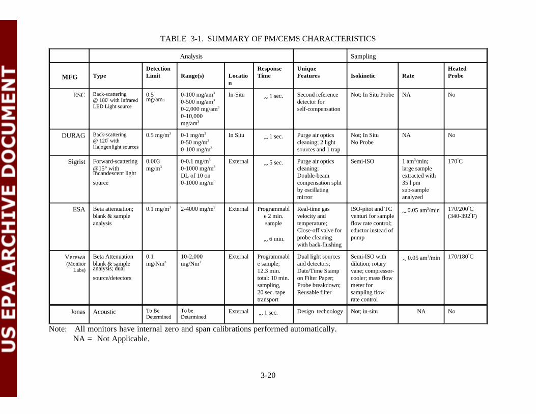
3-20

TABLE 3-1. SUMMARY OF PM/CEMS CHARACTERISTICS

Analysis Sampling

MFG Type Limit Range(s) Locatio Time Features Isokinetic Rate ProbeDetection Response Unique Heated

n

ESC Back-scattering @ 180 with Infrared°

LED Light source

0.5 0-100 mg/am In-Situ Second reference Not; In Situ Probe NA No0-500 mg/am detector for 3

3

mg/am 3

0-2,000 mg/am self-compensation3

0-10,000mg/am3

1 sec.~

DURAG Back-scattering@ 120 with °

Halogenlight sources

0.5 mg/m 0-1 mg/m In Situ Purge air optics Not; In Situ NA No3 3

0-50 mg/m cleaning; 2 light No Probe3

0-100 mg/m sources and 1 trap3

1 sec.~

Sigrist Forward-scattering 0.003 0-0.1 mg/m External Purge air optics Semi-ISO 1 am /min; 170 C@15° with mg/m 0-1000 mg/m cleaning; large sample

DL of 10 on Double-beam extracted withsource 0-1000 mg/m compensation split 35 l pm

3

Incandescent light

3

3

3

5 sec.~

by oscillating sub-samplemirror analyzed

3 °

ESA Beta attenuation; 0.1 mg/m 2-4000 mg/m External Programmabl Real-time gas ISO-pitot and TC 170/200 Cblank & sample e 2 min. velocity and venturi for sample (340-392 F)analysis sample temperature; flow rate control;

3 3

6 min.~Close-off valve for eductor instead ofprobe cleaning pumpwith back-flushing

0.05 am /min~3 °

°

Verewa(Monitor blank & sample mg/Nm mg/Nm e sample; and detectors; dilution; rotary

Labs)

Beta Attenuation 0.1 10-2,000 External Programmabl Dual light sources Semi-ISO with 170/180 C

12.3 min. Date/Time Stamp vane; compressor-source/detectors total: 10 min. on Filter Paper; cooler; mass flow

3

analysis; dual3

sampling, Probe breakdown; meter for20 sec. tape Reusable filter sampling flowtransport rate control

0.05 am /min~3 °

Jonas Acoustic To Be To be Determined Determined

External Design technology Not; in-situ NA No 1 sec.~

Note: All monitors have internal zero and span calibrations performed automatically.NA = Not Applicable.

3-213-21

measuring the same location on the filter tape twice in succession, without collecting a sample. The

span calibration is checked using a radiation attenuator inserted into the measurement beam. For

most of the test program, it took two (2) minutes for sample collection on the filter, two (2)

minutes for filter analysis, and about 60 seconds for filter tape transport time. Using the dual

source/detector configuration, measurements are thus reported about every 12.3 minutes in the

beginning and 5 to 6 minutes at the end of this test program. These times are programmable,

however, so different sample and reporting times can be obtained depending on the sample loading.

3.3.2 Emissions SA 5M Beta Gauge Monitor

The Emissions SA Beta 5M uses a heated sampling probe with real-time pitot and

thermocouple measurements to obtain an isokinetic sample that is maintained automatically. These

features are suitable for applications where moisture/acid-gas dew points are approached and/or

where larger particles ( >5 microns) prevail. The sample is collected on a filter, which, at the end of

the sampling period, is moved using a continuous filter tape mechanism to a measurement location

between a carbon 14 beta particle source and a detector. The beta transmission through each blank

filter is determined before sampling begins. The sampling duration is programmable and determines

the mass concentration detection limit. At high PM loadings, it must be kept small enough to prevent

sampling excessive amounts of PM, and is usually set at two (2) minutes for typical applications.

Analysis takes 90-120 seconds, and thus a measurement is made every six (6) minutes. At the end

of each sampling period, the probe nozzle is temporarily closed, opened, and closed again in order

to re-entrain any PM deposited in the probe. It is equipped with a programmable logic controller

which monitors and diagnoses key sampling and analysis operations. The instrument is relatively

insensitive to variations in PM composition and properties, thus a site-specific calibration is not

generally required, although certification tests are normally performed.

3.3.3 Durag DR-300 Light-scattering Monitor

The Durag model D-R 300-40 light-scattering monitor measures the back scattered light at

approximately 120 by the PM. The light beam is generated by a halogen lamp (400-700 nm)

3-223-22

modulated at 1.2 kHz, and the sample volume is located in a region 80 to 280 mm (centered at 150

mm) from the wall. Both the light source and the detector are located in a single unit, thus requiring

only one point of access to the duct and light trap on opposite side of stack. The D-R 300-40 is

designed to carry out and record automatic zero and span checks, and it provides automatic

compensation for dirt on the optics even though the optics are protected by an air purge system.

Stray light from surface reflections of the transmitted beam is minimized through the use of a light

trap mounted on the opposite side of the duct. The D-R 300-40 is normally located directly on the

duct wall, thus making an in-situ measurement.

For applications where moisture/acid-gas dew points are approached, a hot by-pass system

is available but not provided for this demonstration.

3.3.4 ESC P5A Light-scattering Monitor

Environmental Systems Corporation model P5A light-scattering instrument monitors the back

scattered light (180 ) from an infrared light emitting diode (LED). The instrument has a roughly

constant response to particles in the 0.1 to 10 micron range and a measurement range of 1 to 10,000

mg/dscm. The measuring area is located 4.5 inches from the end of a probe containing both the

transmitting and receiving optics that are inserted into the flow through a standard flange. The probe

is purged with its own blower, supplying air to keep the optics clean. Only one point of access and

light trap to the stack is required; measurement is accomplished in-situ without an extractive probe.

The instrument automatically carries out and records zero and span calibrations and is continuously

compensated for any changes in the LED intensity due to aging or temperature changes via a second

reference detector. A site-specific calibration is recommended to assure accuracy.

3.3.5 Sigrist KTNR Light-scattering Monitor

The Sigrist model KTNR is an extractive sampling light-scattering monitor suitable for

3-233-23

applications where moisture/acid-gas dew points are approached or produced. This device extracts

a heated slipstream (1 m /min) from the stack, a small portion of which is sampled (35 liters/min) and3

passes through a scattered light photometer. The entire sample, including the bypass portion of the

slipstream, is then returned to the duct. The sample rate is set up to be close-to-isokinetic at a normal

stack flow, but isokinetic sampling is not actively maintained. Rather, a constant sample rate is

maintained. The photometer measures the forward light scattered at 15 from a incandescent bulb

emitting over the range 360 to 2800 nm. A double beam compensation measuring method is used

in which the light path is split and the intensity of the reference path adjusted by an attenuator to

equal the intensity of the measurement path. The amount of adjustment necessary is reflected in the

output signal. This approach makes the output signal independent of fluctuations or aging in the

optical and electronic components, including the buildup of dirt on the optics. Drift of the calibration

and zero point is absent. Periodic cleaning and checks with optical filters supplied with the instrument

are carried out, typically in 6 to 12 months. Measuring ranges run from 0 to 0.1 mg/dscm to 0 to

1000 mg/dscm. It is recommended that a site-specific calibration be performed to improve accuracy.

3.3.6 Jonas, Inc.

The Jonas Consulting Acoustic Energy PM monitor uses shock waves caused by the impact

of particles with a probe inserted into the flow to measure particle loading. The device counts the

number of impacts and also measures the energy of each impact. This information, coupled with

knowledge of the flow velocity, allows calculation of the particle mass. Since the probe distorts the

flow, changes in flow velocity and particle size distribution will, in principle, change the instrument

response. However, correction for the flow pattern is included in the instrument’s response.

3.3.7 CEMS Data Acquisition System

All the data from the CEMS instruments are collected and stored on a dedicated data

acquisition system (DAS) manufactured by Environmental Systems Corp. This system includes a data

logger with a personal computer and a modem for automatic downloading of data. The DAS is

3-243-24

housed in an air-conditioned and weather-proofed cabinet located on the stack sampling platform,

as shown in Figures 3-5 and 3-6. The data logger samples each CEMS signal output (typically 4 to

20 milliamp) once per second and calculates one minute averages based on these samples. The one-

minute averages are further used to produce 10- and 60-minute rolling averages. Additional channels

are available for other inputs, such as stack gas temperature, O , and moisture.2

3.4 Scanning Electron Microscope Analytical Procedure

Each filter from the September and October tests was assigned a sequential laboratory

number. A wedge-shaped sample was cut from the filter and mounted on an aluminum planchet using

silver paint. Each sample was analyzed using a JEOL JSM 840A Scanning Electron Microscope

(SEM). The filters were scanned using Backscattered ED Electron Microscopy (BEM). A

compositional image was selectively obtained using a paired semiconductor element conductor in the

BEM. This form of microscopy was very useful for surveying sample surfaces prior to X-ray

analysis.

A photo micrograph was taken of a selective portion of each sample which appeared to

represent most of the particles collected on the filter. These photos were taken using BEM. Particles

with elements of high atomic numbers produced bright images in the photomicrograph.

Energy-Dispersive X-ray (EDX) analysis was performed on the various particle types found

on each sample. Electrons produced during EDX analysis emit unique and characteristic patterns of

X-rays. Under analytical conditions, the number of X-rays emitted by each element reflects its

concentration.

A second series of analyses was performed on wedges of selected filter samples that were

utilized in the November monthly calibration tests. Though similar to the first series of analyses

which provided a general assay with qualitative results, the purpose of the second set of analyses was

to produce semi-quantitative results of the relative amounts of the elements (excluding oxygen)

found in the spectral analysis of the collected PM on the filter samples.

3-253-25

This second series of analyses consisted of SEM, EDS, and Advanced Image Analysis (AIA)

with two (2) photomicrographs of each sample analyzed. The samples were prepared for analysis by

slicing a pie wedge corresponding to about 1/5 of the total filter area and mounting the wedge on a

carbon planchet with carbon paint. Imaging occurred at a magnification of 100x at 20 kilovolts. The

SEM/EDS automated imaging program analyzed each wedge sample for up to 15 elements and

produced high resolution X-ray maps for each element detected. This innovative analytical technique

produced:

- Semi-quantitative data of the relative amounts of the elements found,

- Photomicrographs at 100x of the field examined, and

- A second series of photomicrographs displaying respective distributions of each element

found.

3.5 Process Data Acquisition

Process data are manually recorded from the facility operating system are included in the

Appendix.

4-14-1

4.0 QUALITY ASSURANCE/QUALITY CONTROL

Quality Assurance Program

Quality assurance is an integrated system of activities which involves planning, quality control,

quality assessment, reporting, and quality improvement to ensure that the test program meets

standards of quality with a stated level of confidence. Quality assurance encompasses the

organization within which quality control activities are performed. The QC activities which

accompany testing, lab analysis and other procedures provide control of data and quantify the quality

of data so that it meets the needs of the users as stated in the quality assurance objectives.

Generally, EER's QA procedures follow the guidelines in the “Quality Assurance Handbook

for Air Pollution Measurement Systems,” Volumes I through III. These procedures outline pre-test

preparation and calibrations of sampling equipment, post-test sample handling, and post-test

calibrations. Standardized, written procedures, calculator programs, and spreadsheets are used for

test planning, pre-surveys, equipment checklists, preliminary calculations, data and sample collection,

sample tracking, sample and data analysis, and reporting.

Test procedures were based on applicable EPA test methods. However, slight modifications

of the standard Method 5 filter holder assembly and filter recovery procedure were made to improve

quality of the Method 5i data. For each key measurement area, there were specific QC activities and

checks to ensure that written procedures were followed during all preparation, validation, sampling,

and recovery activities. There are also criteria to quantify and judge the performance of the

measurements and corrective action procedures for correcting deficiencies. Prior to reporting, all

data was reviewed by an independent QA auditor.

Quality Assurance Approach

4-24-2

The EPA has defined Categories I through IV to define the content of QA plans according

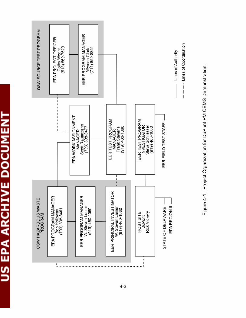
4-34-3

4-44-4

to the goals of the program with which the QA plan is associated (Preparation Aids for the

Development of RREL Quality Assurance Project Plans, U.S. EPA, Risk Reduction Engineering

Laboratory, Cincinnati, OH, 1989). The four categories are defined as follows:

Category Description

I Projects for support of enforcement, compliance, or litigation. This level of QA is the

highest possible for legal challenge. The cost of the QA program for this type of

project is typically 20-30% of the total cost.

II Projects for producing results used to complement (or in combination with) other

projects of similar scope for rule making, regulation making, or policy making. Data

quality indicators (DQIs) for completeness, representativeness, and comparability may

not be easily defined. The cost of the QA program for this type of project is typically

10-30% of the total cost.

III Projects for producing results used for engineering, technology development,

feasibility studies, or preliminary assessments. QA requirements are more broadly

defined, although definitive documentation of QC activities and results is still required

for reports.

IV Projects for producing results used in assessing suppositions, feasibility studies, or

fundamental investigations.

The purpose of this test program was to generate data to evaluate: (1) the acceptability of

commercially-available PM CEMS towards the Draft Performance Specification 11, (2) the

applicability of those draft performance specifications, and (3) the acceptability of modifying Method

5 for measuring low PM emission levels. Category I QA/QC was implemented during this

program. Phase I required an abbreviated form of the QA/QC required in a Category II program

4-54-5

since fewer samples were collected than are required to calculate the necessary DQIs.

QA/QC Organization

The QA/QC structure for this test project is shown in Figure 4-1. The Test Program

Investigator was Mr. Steve Schliesser of EER. EER’s Quality Assurance Officer is Mr. Jerry Cole,

and EER Project QA Coordinator was Mr. Bob Zimperman. Mr. Zimperman had overall

responsibility for all project QA. The QA Coordinator’s activities consisted of test plan review, on-

site performance and system audits, analytical system and performance audits, and reporting of all

QA/QC activities and data. The efforts of the QA coordinator were designed to assure that the

specific goals for precision, accuracy, and completeness were achieved. In addition, an outside

independent QA consultant performed a comprehensive audit of all data produced during the tests.

4.1 Quality Assurance Objectives

Quality assurance objectives are goals for test data accuracy, precision, and completeness.

Accuracy is the degree of agreement of a measurement (or average of measurements) with an

accepted reference or true value. Precision is a measure of mutual agreement of replicate

measurements. Completeness is a measure of the amount of valid data compared to the amount that

was expected to be obtained under correct operating conditions. QA objectives should be defined

for all of the critical measurements of the test program. The objectives should be based on the

limitations and requirements of the test methods, where available. The quality assurance objectives

for the particulate matter are: completeness of 98%; precision of a constant weighing ± 1% or ± 0.5

mg, whichever is greater; and accuracy of ± 6%.

Some of the data validation was not completed until after the testing phase ended. In this

case, it may not be possible to take corrective action to meet the quality assurance objectives (for

example, if the analytical laboratory irrecoverably contaminates or loses a sample). Daily records

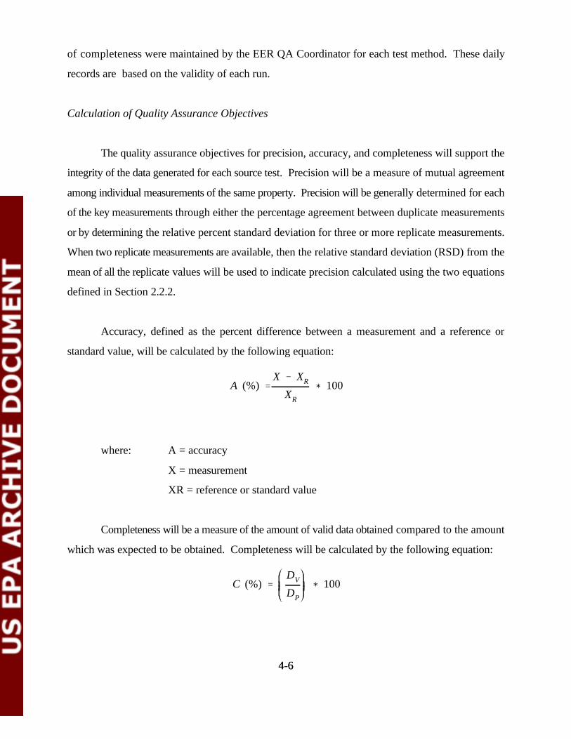
A (%)X XR

XR

100

C (%)DV

DP

100

4-64-6

of completeness were maintained by the EER QA Coordinator for each test method. These daily

records are based on the validity of each run.

Calculation of Quality Assurance Objectives

The quality assurance objectives for precision, accuracy, and completeness will support the

integrity of the data generated for each source test. Precision will be a measure of mutual agreement

among individual measurements of the same property. Precision will be generally determined for each

of the key measurements through either the percentage agreement between duplicate measurements

or by determining the relative percent standard deviation for three or more replicate measurements.

When two replicate measurements are available, then the relative standard deviation (RSD) from the

mean of all the replicate values will be used to indicate precision calculated using the two equations

defined in Section 2.2.2.

Accuracy, defined as the percent difference between a measurement and a reference or

standard value, will be calculated by the following equation:

where: A = accuracy

X = measurement

XR = reference or standard value

Completeness will be a measure of the amount of valid data obtained compared to the amount

which was expected to be obtained. Completeness will be calculated by the following equation:

4-74-7

where: C = Completeness

Dv = Quantity of valid data

Dp = Quantity of expected data

4.2 Reference Method QC

The quality assurance (QA) objectives provide a standard of quality for the various

measurements to be made in this program. These objectives include criteria for precision, accuracy,

and completeness. In order to quantify how well the measurements have satisfied these objectives,

comprehensive internal QA/QC activities were implemented. The efforts of the internal QA

coordinator are designed to assure that the specific goals for precision, accuracy, and completeness

are achieved. The specific system of internal quality control (QC) procedures to establish the

performance of the measurement systems is presented in this section. This system of internal checks

is an integral part of the emissions characterization program.

For each key measurement area, there were specific QC activities and checks, which ensure

that written procedures are followed during all preparation, validation, sampling, and recovery

activities. There are also criteria used to quantify and judge the performance of the measurements

and corrective action procedures for correcting deficiencies, if necessary.

Quality control is the overall system of activities whose purpose is to provide a quality

product or service: for example, the routine application of procedures for obtaining prescribed

standards of performance in the monitoring and measurement process. Quality assurance, on the

other hand, is a system of activities whose purpose is to provide assurance that the QC system is

adequate to ensure that the program goals will be achieved and that it is being implemented

effectively. The program quality control system includes these features:

• Calibration procedures and schedules;

4-84-8

• Specific checklists and procedures for pre-test, test operation, and post-test activities

for each measurement system;

• Standard pre-programmed calculation routines using hand-held calculators and

computer spreadsheets;

• Blanks, spikes, duplicates, QC audit samples, and other analytical quality control

procedures for each measurement system; and

• Organization and documentation of all calibration records, run, data, and calculation

sheets, process logs, spreadsheet files, and printouts.

QA audits were conducted in order to ensure that the above QC activities were effectively

implemented. The following sub-sections discuss QC activities ensuring data validity.

Quality control samples are used to determine QA objectives and to provide data which

supports the generated data. Quality control samples include field blanks, matrix spikes, matrix spike

duplicates, and laboratory control spikes.

4.2.1 Quality Control Procedures

This program involved sampling and analysis of the stack outlet flue gas stream. This section

describes the QA/QC activities and criteria accomplished during the sampling, as well as the analytical

phases of this test program.

4.2.2 QC for Flue Gas Sampling and Analysis

The following section discusses the QA/QC activities utilized for this program’s flue gas

sampling and analytical procedure.

EPA Method 1, 2, and 4 - Sample point determination, flue gas velocity, and moisture content

4-94-9

Sampling: The S-type pitot tube was visually inspected before sampling. Both legs of the pitot

tube were leak checked before and after sampling. Proper orientation of the S-type

pitot tube was maintained while making measurements. The roll and pitch axis of the

S-type pitot tube is maintained at 90 to the flow. The oil manometer was leveled

and zeroed before each run. The pitot tube/manometer umbilical lines were inspected

before and after sampling for moisture condensate. Cyclonic or turbulent flow checks

were performed prior to and after the test program. An average velocity pressure

reading was recorded at each point instead of recording extreme high or low values.

Reported duct dimensions were checked by measurements to determine cross-

sectional duct area. If a negative gas static pressure was present, checks were made

for air in leakage at ports resulting in possible flow and temperature errors (leaks were

sealed if found). The stack gas temperature measuring system was checked by

observing ambient temperatures prior to placement in the stack. The balance zero was

checked, and rezeroed if necessary, before each weighing. Pre-test liquid volumes of

impinger solutions were recorded as a check on tare weights. The balance was

leveled and placed in a clean, motionless environment for weighing. The indicating

silica gel was fresh for each run and periodically inspected and replaced during runs

if necessary. The silica gel impinger gas temperature was maintained below 68 F.

The dry gas meter is fully calibrated using an EPA-approved intermediate standard.

Pre-test, port change, and post-test leak checks are completed (must be less than 0.02

cfm or 4% of the average sample rate). The gas meter was read to the thousandth of

a cubic foot for the initial and final readings. The meter thermocouples were

compared with ambient prior to the test run as a check on operation. Readings of the

dry gas meter, meter orifice pressure ( H) and meter temperatures were taken at

every sampling point. Accurate barometric pressures were recorded at least once a

day.

Analysis: Prior to daily use, the balance was calibrated with NIST-traceable weights. The

impingers were weighed to the nearest 0.5 g.

4-104-10

EPA Draft Method 5

Sampling: All sampling equipment was thoroughly checked to ensure clean and operable

components. The oil manometer or Magnehelic gauge used to measure pressure

across the S-type pitot tube was leveled and zeroed. The pitot tubes and connecting

tubing were leak checked. The temperature measurement system was visually

checked for damage and operability by measuring the ambient temperature prior to

each traverse. All train components were sealed with Teflon tape before train was

leaked checked.

During Test: Duplicate readings of temperature and differential pressure were taken

at each traverse point. Isokinetic sampling rates were maintained at each traverse

point. The sample train was leak-checked between most port changes.

The probe and filter temperature were maintained at 248 (± 25) F. The impinger

outlet temperature was maintained at < 68 F. Any unusual occurrences were noted

during each run on the appropriate data form.

Post-test: The Field Team Leader reviewed sampling data sheets daily after testing.

Each train operator recorded final gas meter readings; performed a final leak-check

at the highest observed vacuum; ensured that the Field Task Manager had the data

sheets; and transported samples to recovery area.

Analysis: Method 5 QC samples collected in the field included a field train blank and field

acetone blanks. Sample results were corrected for field reagent blanks only as

described in Method 5. The field train blank results are reported with the sample

results.

Analysis of particulate in Method 5 samples were conducted by a microbalance with

4-114-11

resolution of ± 0.1 mg for weights less than 100 g. The balance was calibrated prior

to analysis using NIST-traceable Class S weights. The calibration was checked using

one of the Class S weights. Table 4-1 lists the QA/QC criteria for the stack gas

sampling procedure.

4.3 Field Data Reduction

Data gathered during this program falls into the following categories:

1. Manual methods sampling operations data and sample analysis data; and

2. Process data.

Manual methods operations data were input to computer spreadsheets each day following

receipt from testing. Results of samples analysis were input to the computer system upon receipt

from analytical labs. Process data consisted of logs and continuously monitored data. Data was

reduced and analyzed using hand-held calculator programs, computer spreadsheets, and other

computer programs. The actual equations and nomenclature are shown on the calculator program

data sheets and on the spreadsheets. This feature enables operator and analyst familiarity with the

programmed computations, gives facilities separate spot-checking of computed results by hand, and

eliminates the need to show equations separately in the text.

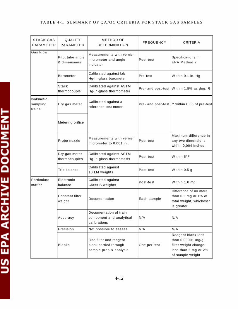
TABLE 4-1. S U M M A R Y O F Q A / Q C C R I T E R I A F O R S T A C K G A S S A M P L E S

STACK GAS PARAMETER

QUALITY PARAMETER

METHOD OF DETERMINATION

FREQUENCY CRITERIA

Gas FlowPitot tube angle & dimensions

Measurements with vernier micrometer and angle indicator

Post-testSpecifications in EPA Method 2

BarometerCalibrated against lab Hg-in-glass barometer

Pre-test W ithin 0.1 in. Hg

Stack thermocouple

Calibrated against ASTM Hg-in-glass thermometer

Pre- and post-test W ithin 1.5% as deg. R

Isokinetic sampling trains

Dry gas meterCalibrated against a reference test meter

Pre- and post-test Y within 0.05 of pre-test Y; delta H@ within 0.15 of pre-test

Metering orifice

Probe nozzleMeasurements with vernier micrometer to 0.001 in.

Post-testMaximum difference in any two dimensions within 0.004 inches

Dry gas meter thermocouples

Calibrated against ASTM Hg-in-glass thermometer

Post-test W ithin 5°F

Trip balanceCalibrated against 10 LM weights

Post-test W ithin 0.5 g

Particulate matter

Electronic balance

Calibrated against Class S weights

Post-test W ithin 1.0 mg

Constant filter weight

Documentation Each sample

Difference of no more than 0.5 mg or 1% of total weight, whichever is greater

AccuracyDocumentation of train component and analytical calibrations

N/A N/A

Precision Not possible to assess N/A N/A

BlanksOne filter and reagent blank carried through sample prep & analysis

One per test

Reagent blank less than 0.00001 mg/g; filter weight change less than 5 mg or 2% of sample weight

4-124-12

4-134-13

4.3.1 Manual Method 5i Data Reduction

Standardized run data forms were used for each method. All run sheets were reviewed daily

by the Field Manager for evaluation of progress, completeness, and problems. Standardized

computer spreadsheets were used to reduce and analyze field data. At the end of each test day, test

data was input to these spreadsheets. Lab analytical results were not available at the end of each test

day. However, analytical results were input as they became available. A standard data set, which

has been verified by hand, was used to demonstrate the accuracy of the spreadsheet calculations

before and after the test program.

For each manual method, the field data were reduced manually at the end of each run. An

isokinetic ratio was then estimated at the end of each run using an average, typical, or dry/wet bulb

measured moisture value. The estimated moisture value, estimated isokinetic ratio, and all

intermediate calculations were noted on the run sheet. Upon entry into the computer spreadsheet

program, both the data and the program were checked by comparing the estimated isokinetic ratio

against the spreadsheet determined value.

Spreadsheet calculations for the various runs observed the following guidelines:

1. Isokinetic calculations for each train were conducted using the input run data from

that specific run rather than from the average or other values from previous runs.

Stack gas moisture content was determined using the condensed water measured in

that train; and

2. Stack temperature, moisture content, velocity, and flow rate values for each train

were averaged.

The accepted range for the isokinetic rate is 90 to 110%. Data outside this range were

discarded.

4-144-14

Upon daily completion of testing, the Field Manager was responsible for preparation of a data

summary which will include each of the following for each run:

• Raw data sheets;

• Calculation of isokinetic ratio for each run;

• Traverse start and stop times for each run;

• Calculation of sample volume for each run;

• Calculation of stack gas flow rate; and

• Problems encountered during sampling and/or deviations from standard procedure.

The daily data summary was submitted to the QA Coordinator. The final project report

includes a separate QA/QC section which summarizes any audit results from manual sampling

procedures, as well as, QC data collected throughout the duration of the program. The EER QA/QC

Officer reviewed the manual methods QC data and provided data quality input for the final report.

4.3.2 Data Validation

Data validation is a systematic procedure of reviewing data against a set of established criteria

to provide a level of assurance of its validity prior to intended use. Data were validated internally by

QC personnel. All measurement data were validated based upon process conditions during sampling

or testing, acceptable sample collection/testing procedures as outlined in Section 3, consistency with

expected and/or other results, adherence to prescribed QC procedures, and the specific acceptance

criteria. The data were coded as valid or invalid based on its adherence to these criteria. Data

validation was conducted at several critical stages of data reduction:

• Field checks of raw and reduced field data by the Field Manager and Crew Leaders;

• Analytical laboratory QC Checks by a lab QA Supervisor;

• Spot checks of reduced raw data by the Project QA Coordinator;

• Review of summary tables for consistency with reduced raw data by the Project QA

4-154-15

Coordinator;

• Draft final report review by the QA Manager, Program Manager, Principal

Investigator and Project Manager;

• Final report review by the Program Manager, Principal Investigator, and Project

Manager; and

• A comprehensive review of all input data, spreadsheets, calculations, analytical data,

and general QC procedures by an independent QA consultant.

Data validation consists of verification of calculation methodology, consistency of raw,

reduced and summarized data tables, comparison of expected results, and consistency of results

among multiple measurements at the same location.

Field data were initially validated by the EER Field Manager and the internal QC Coordinator

based on their judgement of the representativeness of the sample, maintenance and cleanliness of

sampling equipment, and the adherence to the sample collection procedures defined in Section 3.

They also validated the data daily based on :

• Process conditions during sampling;

• Adherence to acceptance criteria; and

• Acceptable external performance evaluation and technical system audit results

conducted by an external auditor.

When the data set is complete, the EER field QA Officer performed an overall review of the

data. This review considered:

• The previously listed criteria; and

• The reasonableness and consistency of the data based on a knowledge of the site

characteristics and the specific location of the samples.

The review also contained an evaluation of the data in terms of meeting the quality assurance

objectives of the program discussed in Section 4 of this plan. The QC criteria for data validation

4-164-16

contains consistency, duplicate sample calibration, tests for outliers, transmittal error, and uncertainty

analysis.

Outliers were identified by comparison with other measurements in a set of observations using

the standard student T-Test procedures for outliers. This test flagged specific data points as potential

outliers; however, it did not automatically disqualify any data. Corrective action was initiated

immediately to determine the outlier cause. If possible, the associated sample was reanalyzed. The

acceptance rejection of the data was in a uniform and consistent manner based on the established

validation criterion of paired train RSD values of > 30%. Data were rejected only on that basis.

Validation of spreadsheet calculations used for data reduction was conducted by entering a

QA data set which has been verified by hand. This was done at the beginning and end of the test

program.

Data flags were added to all tables to identify special handling procedures or unusual data

results. These flags included:

• Quantities including analytical results which are at or below method minimum

detection limits;

• Any results where contamination is suspected;

• Any average results which exclude any individual test run results; and

• Other special data handling procedures or qualifications.

4.4 CEMS Data Acquisition/Reduction

The CEMS data are transferred by modem from the site CEMS’s data acquisition system to

the EER office. The data are stored in a holding directory and later printed as an Excel file.

CEMS data taken during the field reference method test are averaged. The data average is

an average of the time the manual method sampling was conducted, minus the period of time needed

for port changes.