DRAFT

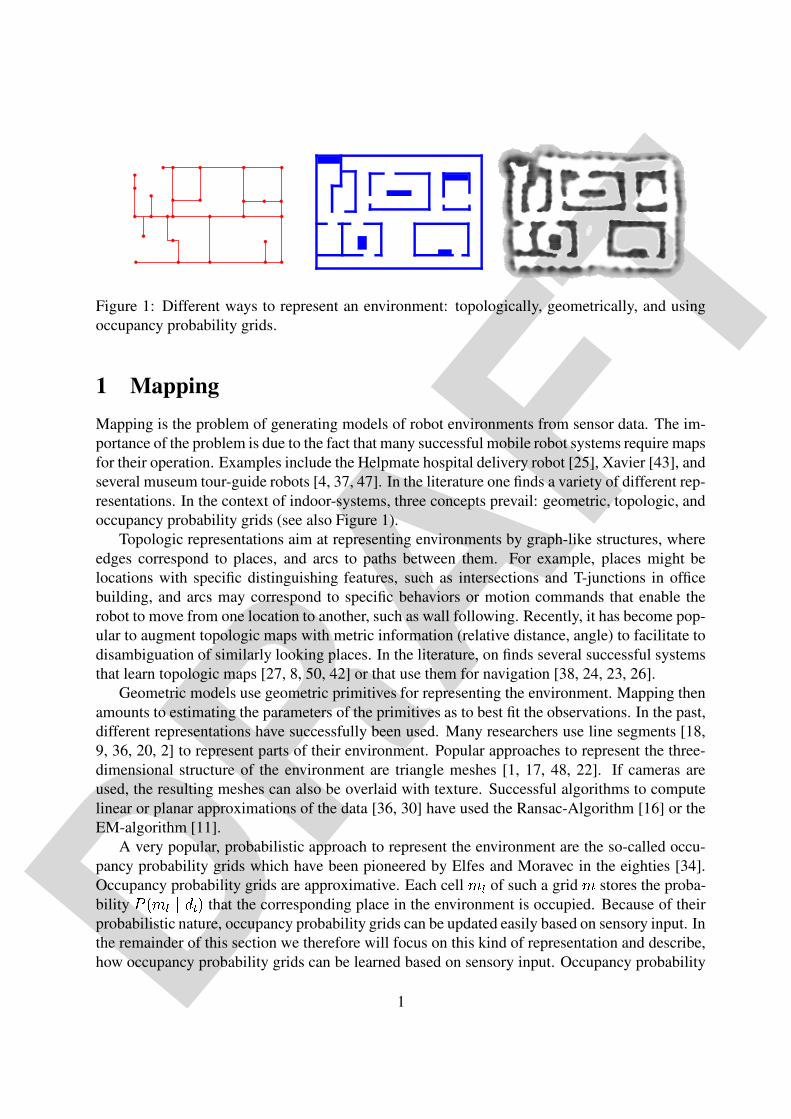
DRAFTFigure 1: Different ways to represent an environment: topologically, geometrically, and usingoccupancy probability grids.

1 MappingMapping is the problem of generating models of robot environments from sensor data. The im-portance of the problem is due to the fact that many successful mobile robot systems require mapsfor their operation. Examples include the Helpmate hospital delivery robot [25], Xavier [43], andseveral museum tour-guide robots [4, 37, 47]. In the literature one finds a variety of different rep-resentations. In the context of indoor-systems, three concepts prevail: geometric, topologic, andoccupancy probability grids (see also Figure 1).

Topologic representations aim at representing environments by graph-like structures, whereedges correspond to places, and arcs to paths between them. For example, places might belocations with specific distinguishing features, such as intersections and T-junctions in officebuilding, and arcs may correspond to specific behaviors or motion commands that enable therobot to move from one location to another, such as wall following. Recently, it has become pop-ular to augment topologic maps with metric information (relative distance, angle) to facilitate todisambiguation of similarly looking places. In the literature, on finds several successful systemsthat learn topologic maps [27, 8, 50, 42] or that use them for navigation [38, 24, 23, 26].

Geometric models use geometric primitives for representing the environment. Mapping thenamounts to estimating the parameters of the primitives as to best fit the observations. In the past,different representations have successfully been used. Many researchers use line segments [18,9, 36, 20, 2] to represent parts of their environment. Popular approaches to represent the three-dimensional structure of the environment are triangle meshes [1, 17, 48, 22]. If cameras areused, the resulting meshes can also be overlaid with texture. Successful algorithms to computelinear or planar approximations of the data [36, 30] have used the Ransac-Algorithm [16] or theEM-algorithm [11].

A very popular, probabilistic approach to represent the environment are the so-called occu-pancy probability grids which have been pioneered by Elfes and Moravec in the eighties [34].Occupancy probability grids are approximative. Each cell ��� of such a grid � stores the proba-bility

��� �������� that the corresponding place in the environment is occupied. Because of theirprobabilistic nature, occupancy probability grids can be updated easily based on sensory input. Inthe remainder of this section we therefore will focus on this kind of representation and describe,how occupancy probability grids can be learned based on sensory input. Occupancy probability

1

DRAFT

grids and variants thereof have also been successfully used to represent the three-dimensionalstructure of the environment [33, 28, 41].

To map an environment, a robot has to cope with two types of sensor noise: Noise in percep-tion (e.g., range measurements), and noise in odometry (e.g., wheel encoders). Because of thelatter, the problem of mapping creates an inherent localization problem, which is the problem ofdetermining the location of a robot relative to its own map. The mobile robot mapping problemis therefore often referred to as the concurrent mapping and localization problem (CML) [29], oras the simultaneous localization and mapping problem (SLAM) [6, 12] (see also Section ??). Infact, errors in odometry render the errors of individual features in the map dependent even if themeasurement noise is independent, which suggests that mapping is a high-dimensional statisticalestimation problem, often with tens of thousands of dimensions. In this chapter we approach thisproblem in two steps. First we concentrate on the question of how to build maps given the poseof the robot is known. Afterwards we relax this assumption and describe a recently developedtechnique for simultaneous mapping and localization.

1.1 Mapping with Known PosesIn this section we will discuss how a mobile robot can learn an occupancy probability grid mapfrom the sensor data given the positions ��� of the vehicle at each point in time � is known.Suppose ����� ����������������� �!� are the position of the robot at the individual steps in time and "#��� ���"$�������%�&"%� are the perceptions of the environment. Occupancy probability grids determine foreach cell of the grid the probability that this cell is occupied by an obstacle. Thus, occupancyprobability grids seek to find the map ' that maximizes (�)*',+��-��� �.�/"$��� �10 . If we apply Bayes ruleusing ����� � and "$��� �32!� as background knowledge, we obtain(4)�'5+6����� �.�&"$��� ��05� (�)�"%�7+8'9�:����� �.�/"$��� �32!� 0�;8(�)*',+8����� ���&"$��� �32!� 0(4)1"%�<+=����� �.�/"$��� �32!� 0 (1)

If we assume that "�� is independent from ����� �32!� and "$��� �32!� given we know ' the right side of thisequation can be simplified to(4)�',+=����� �.�/"$��� ��05� (4)1"%�<+$'9�:�!�10�;8(�)*',+=����� �.�/"$��� �32!� 0(4)1"%�<+=����� �.�/"$��� �32!� 0 (2)

We now again apply Bayes rule to determine(4)1"%�<+8'9� �!�105� (4)�'5+>"%�?� �!�10�;8(�)�"%�7+=�!�@0(4)�'5+=�!�@0 (3)

If we insert Equation (3) into Equation (2) and assuming that and since �A� does not carry anyinformation about ' if there is no observation "=� , we obtain(4)�'B+=����� �.�&"$��� �10,� (�)*'B+6"%�.� �!�10�;8(4)1"%�<+=�!�10�;8(4)�'5+6����� �32!���&"$��� �32!� 0(4)�'C0�;=(4)1"%�<+8����� �.�/"$��� �32!�:0 (4)

2

DRAFT

If we exploit the fact that each DFE:G1H�I is a binary variable, we derive the following equation in ananalogous way.J G1KLDBM=N�O�P E.Q/R$O�P E�I5S J G@KLD,M6R%E.Q N!E1I�T J G�R%E7M=N!E1I�T J G@KLD,M=N�O�P E3U!O%Q&R$O�P E3U!O:IJ G@KLDCI�T J G1R%E<M=N�O�P E.Q/R$O�P E3U!O I (5)

By dividing Equation (4) by Equation (5), we obtainJ G�D5M8N�O�P E.Q/R$O�P E�IJ G@KLD,M8N�O�P E.Q/R$O�P E*I S J G�DBM6R%E.Q:N!E1I�T J G1KVDCI�T J G�D5M=N�O�P E3U!O�Q/R$O�P E3U!O IJ G1KVD,M6R%E.Q N!E1I�T J G�DCI�T J G@KLDBM8N�O�P E3U!O�Q/R$O�P E3U!OWI (6)

Finally, we use the fact thatJ G1KVXYIVS[Z]\ J G�X^I which yieldsJ G�D5M=N�O�P E.Q/R$O�P E1IZ]\ J G�D5M8N�O�P E.Q/R$O�P E�I S J G�D5M>R%E.Q:N!E1IZ]\ J G�DBM6R%E.Q:N!E1I T Z_\ J G*DCIJ G*DCI T J G*D,M8N�O�P E3U!O�Q/R$O�P E3U!O:IZ_\ J G*DBM=N�O�P E3U!O�Q/R$O�P E3U!O I (7)

If we define `Yababc GdNeI5S J GdNeIZ]\ J GdNeI (8)

Equation (7) turns into`Yababc G�DBM8N�O�P E�Q&R$O�P E1I,S `^afabc G�D,M6R%E.Q N!E1I�T `Yababc G�DCI U!O T `Yababc G�DBM8N�O�P E3U!O�Q/R$O�P E3U!O I (9)

The corresponding gih�j `Yababcrepresentation of Equation (9) isgkh�j `Yababc G�DBM8N�O�P E�Q&R$O�P E1I<Sgih�j `Yababc G*DBM$R%E.Q N!E�I�\lgih�j `Yababc G*DCInmogkh>j `^afabc G�D,M=N�O�P E3U!O�Q/R$O�P E3U!O I (10)

Please note that this equation also has a recursive structure similar to that of the recursiveBayesian update scheme ??. To incorporate a new scan into a given map we multiply its

`Yababc-

ratio with the`Yabafc

-ratio of a local map constructed from the most recent scan and divide it bythe

`Yababc-ratio of the prior. Often it is assumed that the prior probability of D is 0.5. In this case

the prior can be canceled so that Equation (10) simplifies togkh�j `Yababc G�DBM=N�O�P E.Q&R$O�P E1I,S gkh�j `Yababc G�DBM6R%E.Q:N!E1I�mogkh>j `Yabafc G�D,M8N�O�P E3U!O�Q/R$O�P E3U!O:I (11)

To recover the occupancy probability from the`Yababc

representation given in Equation (9) we usethe following law which can easily be derived from Equation (8):J GdNeI5S `Yababc GdNeIZ7m `Yababc GdNeI (12)

This leads to:J G�D5M=N�O�P E.Q/R$O�P E1IS p Z7m G.Z_\ J G*DBM=N!E.Q/R%E1I:IJ G*DBM=N!E.Q/R%E1I T J G�DCIGWZq\ J G�DCI I T Zq\ J G�D5M8N�O�P E3U!O�Q/R$O�P E3U!O IJ G�D5M8N�O�P E3U!O�Q/R$O�P E3U!O:I r U!O (13)

3

DRAFT

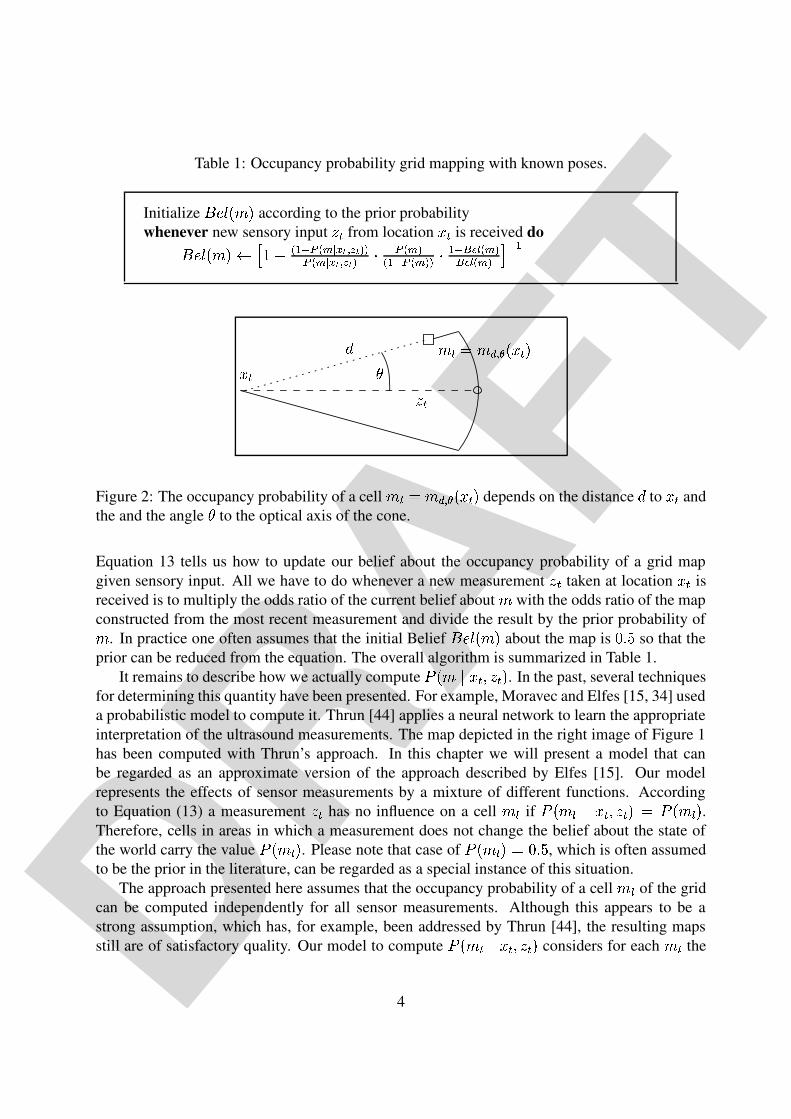
Table 1: Occupancy probability grid mapping with known poses.

Initialize sut=vWw�xCy according to the prior probabilitywhenever new sensory input z={ from location |}{ is received dosut=vWw�xCy�~ �d�<���������A���7� ���1� �@�i����A���7� � � � � � � � �A���L��i�����A���L���V� ����!�@��������!�@��������� �!�

� � � � � � � �� � � � � � � �� � � � � � � �� � � � � � � �� � � � � � � �� � � � � � � �� � � � � � � �� � � � � � � �|!{ � � z%{x �}� xF  � ¡ wd|!{1y

Figure 2: The occupancy probability of a cell x �}� xF  � ¡ wd|!{1y depends on the distance � to |}{ andthe and the angle � to the optical axis of the cone.

Equation 13 tells us how to update our belief about the occupancy probability of a grid mapgiven sensory input. All we have to do whenever a new measurement z6{ taken at location |}{ isreceived is to multiply the odds ratio of the current belief about x with the odds ratio of the mapconstructed from the most recent measurement and divide the result by the prior probability ofx . In practice one often assumes that the initial Belief sut=vWw�xCy about the map is ¢f£�¤ so that theprior can be reduced from the equation. The overall algorithm is summarized in Table 1.

It remains to describe how we actually compute ¥�w*x,¦8|�{.§/z%{1y . In the past, several techniquesfor determining this quantity have been presented. For example, Moravec and Elfes [15, 34] useda probabilistic model to compute it. Thrun [44] applies a neural network to learn the appropriateinterpretation of the ultrasound measurements. The map depicted in the right image of Figure 1has been computed with Thrun’s approach. In this chapter we will present a model that canbe regarded as an approximate version of the approach described by Elfes [15]. Our modelrepresents the effects of sensor measurements by a mixture of different functions. Accordingto Equation (13) a measurement z={ has no influence on a cell x � if ¥�w*x � ¦-|!{.§/z%{1y � ¥�w*x � y .Therefore, cells in areas in which a measurement does not change the belief about the state ofthe world carry the value ¥4w�x � y . Please note that case of ¥4w�x � y � ¢f£¨¤ , which is often assumedto be the prior in the literature, can be regarded as a special instance of this situation.

The approach presented here assumes that the occupancy probability of a cell x � of the gridcan be computed independently for all sensor measurements. Although this appears to be astrong assumption, which has, for example, been addressed by Thrun [44], the resulting mapsstill are of satisfactory quality. Our model to compute ¥4w�x � ¦|!{.§/z%{�y considers for each x � the

4

DRAFT

s

00.5

11.5

22.5measured distance -0.1

-0.05

0

0.05

0.1

theta

0.10.20.30.4

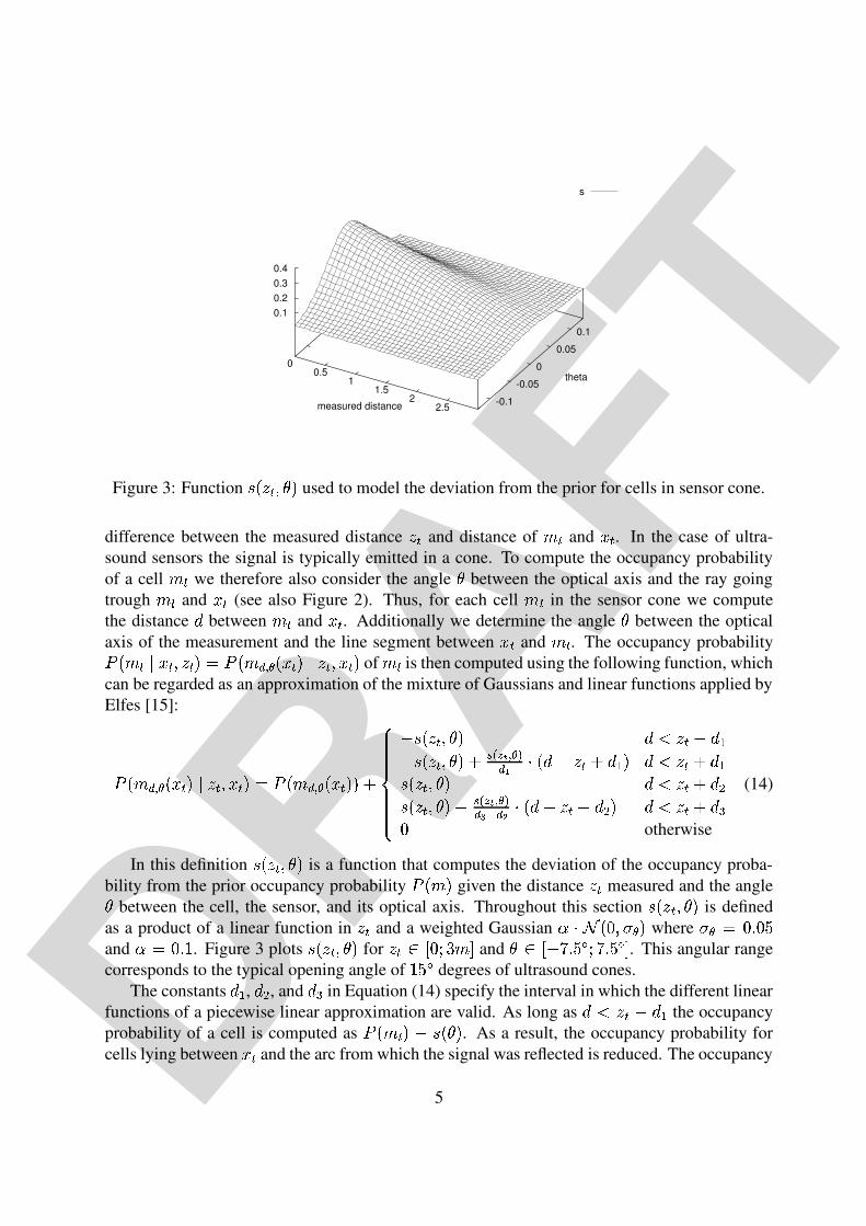
Figure 3: Function ©�ª�«�¬�­/®>¯ used to model the deviation from the prior for cells in sensor cone.

difference between the measured distance «=¬ and distance of °�± and ²!¬ . In the case of ultra-sound sensors the signal is typically emitted in a cone. To compute the occupancy probabilityof a cell °F± we therefore also consider the angle ® between the optical axis and the ray goingtrough °F± and ²!¬ (see also Figure 2). Thus, for each cell °�± in the sensor cone we computethe distance ³ between °�± and ²}¬ . Additionally we determine the angle ® between the opticalaxis of the measurement and the line segment between ²A¬ and °F± . The occupancy probability´ ª�°F±¶µ8²!¬.­/«%¬*¯<· ´ ª*°F¸/¹ º�ª*²!¬1¯»µ6«%¬.­ ²!¬1¯ of °�± is then computed using the following function, whichcan be regarded as an approximation of the mixture of Gaussians and linear functions applied byElfes [15]:

´ ª�°F¸&¹ º8ª*²!¬1¯»µ6«%¬.­ ²!¬1¯V· ´ ª*°F¸/¹ º=ª*²!¬1¯ ¯�¼½¾¾¾¾¾¾¾¿ ¾¾¾¾¾¾¾À

Á ©#ª�«%¬.­/®�¯ ³4Âë%¬ Á ³bÄÁ ©#ª�«%¬.­/®�¯�¼ÆÅ.Ç�È@É ¹ º.ʸ&Ë Ì ª1³ Á «%¬!¼o³bÄW¯5³4Âë%¬b¼Í³fÄ©#ª1«%¬.­/®>¯ ³4Âë%¬b¼Í³ÏΩ#ª1«%¬.­/®>¯ Á Å.Ç�È@É ¹ º.ʸ.Ð Ñ�¸WÒYÌ ª1³ Á «%¬ Á ³ÏÎ�¯ ³4Âë%¬b¼Í³ÏÓÔotherwise

(14)

In this definition ©#ª�«�¬.­/®�¯ is a function that computes the deviation of the occupancy proba-bility from the prior occupancy probability

´ ª*°C¯ given the distance «8¬ measured and the angle® between the cell, the sensor, and its optical axis. Throughout this section ©#ª1«6¬.­/®>¯ is definedas a product of a linear function in «=¬ and a weighted Gaussian Õ Ì�Ö ª Ô ­&×}º/¯ where ×}ºu· ÔfØ�Ô�Ùand ÕÚ· ÔfØ�Û

. Figure 3 plots ©#ª1«�¬�­/®>¯ for «%¬qÜÞÝ Ôfß/à °âá and ®�ÜÞÝ ÁYã بÙ>ä�ß ã بÙ>ä á . This angular rangecorresponds to the typical opening angle of

Û=Ù#ädegrees of ultrasound cones.

The constants ³bÄ , ³ÏÎ , and ³ÏÓ in Equation (14) specify the interval in which the different linearfunctions of a piecewise linear approximation are valid. As long as ³åÂæ«6¬ Á ³bÄ the occupancyprobability of a cell is computed as

´ ª�°C±�¯ Á ©�ª�®�¯ . As a result, the occupancy probability forcells lying between ²}¬ and the arc from which the signal was reflected is reduced. The occupancy

5

DRAFT0

0.2

0.4

0.6

0.8

1

0 0.5 1 1.5 2 2.5 3

p

distance

ç èç è�éuê�ëç è�ìíê�ë5ç:èÏì�ê%î

ç èÏì�ê%ïððð�ð ð

Occupancy probability

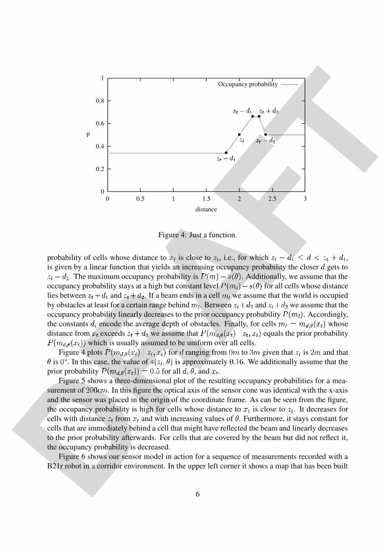
Figure 4: Just a function.

probability of cells whose distance to ñ�ò is close to ó%ò , i.e., for which ó�ò¶ôöõb÷ùøúõüûýó%ò�þÞõf÷ ,is given by a linear function that yields an increasing occupancy probability the closer õ gets toó%òþlõf÷ . The maximum occupancy probability is ÿ�������þ������ . Additionally, we assume that theoccupancy probability stays at a high but constant level ÿ���� ���Ïþ������ for all cells whose distancelies between ó�ò�þ�õf÷ and ó%ò�þ�õ�� . If a beam ends in a cell ��� we assume that the world is occupiedby obstacles at least for a certain range behind ��� . Between ó%ò/þíõ�� and ó%ò/þíõ�� we assume that theoccupancy probability linearly decreases to the prior occupancy probability ÿ�������� . Accordingly,the constants õ�� encode the average depth of obstacles. Finally, for cells � ��������� !�*ñ!ò� whosedistance from ñ!ò exceeds ó�ò�þ õ�� we assume that ÿ�������� !�dñ!ò�#"$ó%ò%$ ñ!ò�� equals the prior probabilityÿ�������� !�*ñ!ò�&� which is usually assumed to be uniform over all cells.

Figure 4 plots ÿ�������� !�dñ!ò�'">ó%ò%$ ñ!ò� for õ ranging from (�� to )�� given that ó�ò is *+� and that is (�, . In this case, the value of �-��ó=ò%$.�� is approximately (0/2143 . We additionally assume that theprior probability ÿ�������� 4�*ñ!ò�&�5�6(0/87 for all õ , , and ñ}ò .

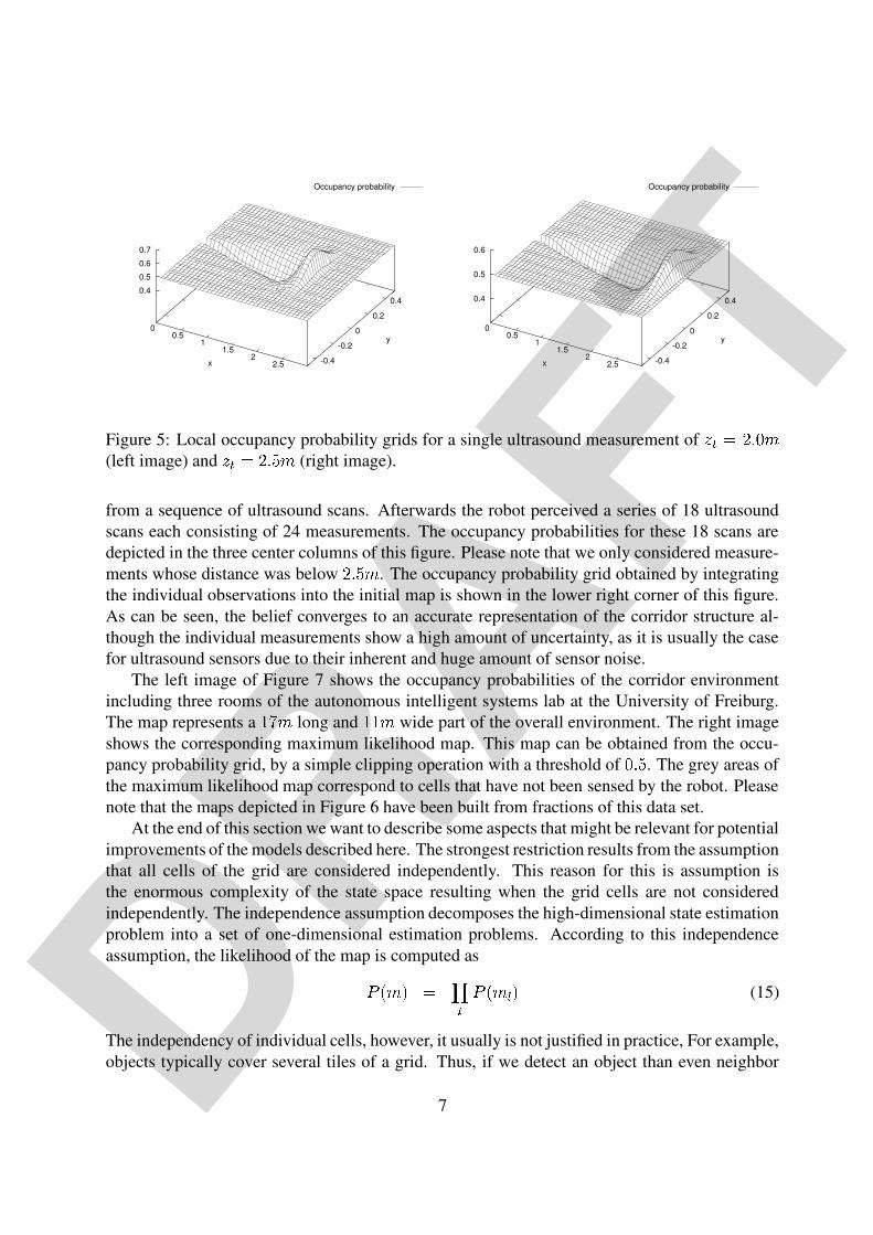
Figure 5 shows a three-dimensional plot of the resulting occupancy probabilities for a mea-surement of *�(�(�9:� . In this figure the optical axis of the sensor cone was identical with the x-axisand the sensor was placed in the origin of the coordinate frame. As can be seen from the figure,the occupancy probability is high for cells whose distance to ñeò is close to ó�ò . It decreases forcells with distance ó�ò from ñ!ò and with increasing values of . Furthermore, it stays constant forcells that are immediately behind a cell that might have reflected the beam and linearly decreasesto the prior probability afterwards. For cells that are covered by the beam but did not reflect it,the occupancy probability is decreased.

Figure 6 shows our sensor model in action for a sequence of measurements recorded with aB21r robot in a corridor environment. In the upper left corner it shows a map that has been built

6

DRAFT

Occupancy probability

00.5

11.5

22.5x -0.4

-0.2

0

0.2

0.4

y

0.4

0.5

0.6

0.7

Occupancy probability

00.5

11.5

22.5x -0.4

-0.2

0

0.2

0.4

y

0.4

0.5

0.6

Figure 5: Local occupancy probability grids for a single ultrasound measurement of ;+<�=�>@?BA�C(left image) and ;D<E=6>@?GFHC (right image).

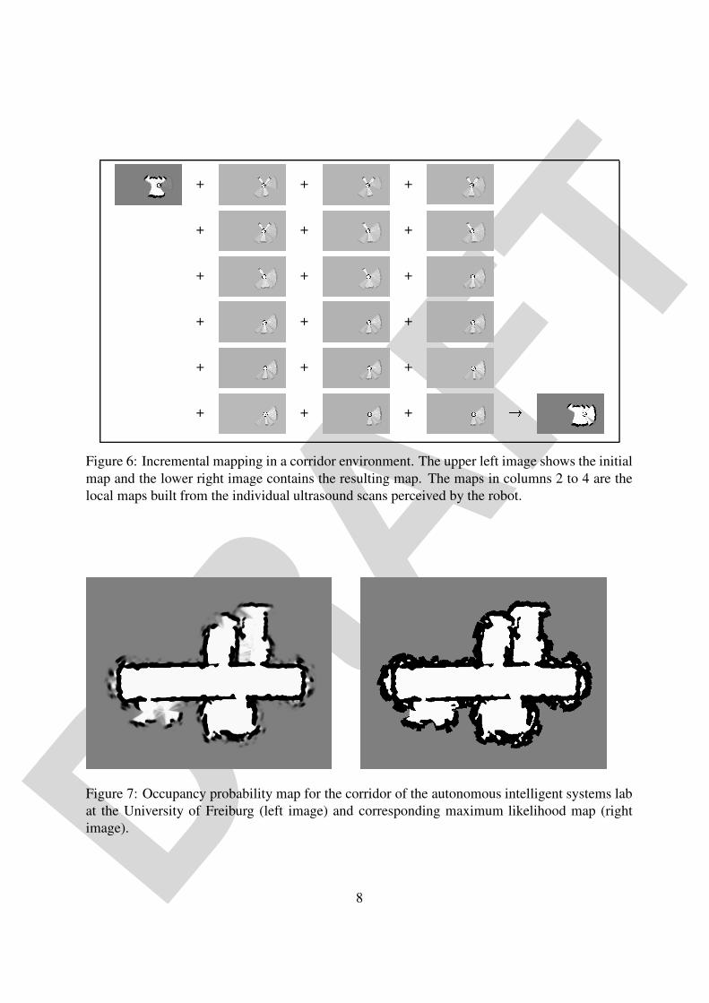
from a sequence of ultrasound scans. Afterwards the robot perceived a series of 18 ultrasoundscans each consisting of 24 measurements. The occupancy probabilities for these 18 scans aredepicted in the three center columns of this figure. Please note that we only considered measure-ments whose distance was below >@?GFHC . The occupancy probability grid obtained by integratingthe individual observations into the initial map is shown in the lower right corner of this figure.As can be seen, the belief converges to an accurate representation of the corridor structure al-though the individual measurements show a high amount of uncertainty, as it is usually the casefor ultrasound sensors due to their inherent and huge amount of sensor noise.

The left image of Figure 7 shows the occupancy probabilities of the corridor environmentincluding three rooms of the autonomous intelligent systems lab at the University of Freiburg.The map represents a I4J+C long and I�IDC wide part of the overall environment. The right imageshows the corresponding maximum likelihood map. This map can be obtained from the occu-pancy probability grid, by a simple clipping operation with a threshold of A0?8F . The grey areas ofthe maximum likelihood map correspond to cells that have not been sensed by the robot. Pleasenote that the maps depicted in Figure 6 have been built from fractions of this data set.

At the end of this section we want to describe some aspects that might be relevant for potentialimprovements of the models described here. The strongest restriction results from the assumptionthat all cells of the grid are considered independently. This reason for this is assumption isthe enormous complexity of the state space resulting when the grid cells are not consideredindependently. The independence assumption decomposes the high-dimensional state estimationproblem into a set of one-dimensional estimation problems. According to this independenceassumption, the likelihood of the map is computed asK�L C�MN= O.P K�L C P M (15)

The independency of individual cells, however, it usually is not justified in practice, For example,objects typically cover several tiles of a grid. Thus, if we detect an object than even neighbor

7

DRAFT

+ + +

+ + +

+ + +

+ + +

+ + +

+ + + QFigure 6: Incremental mapping in a corridor environment. The upper left image shows the initialmap and the lower right image contains the resulting map. The maps in columns 2 to 4 are thelocal maps built from the individual ultrasound scans perceived by the robot.

Figure 7: Occupancy probability map for the corridor of the autonomous intelligent systems labat the University of Freiburg (left image) and corresponding maximum likelihood map (rightimage).

8

DRAFT

cells and not only cells behind the tile in which the beam ends might have a high occupancyprobability. Accordingly, techniques considering the individual cells of a grid independently,might produce sub-optimal solutions. One technique that addresses this problem has recentlybeen presented by Thrun [46]. Additionally, occupancy probability grid maps assume that theenvironment has a binary structure, i.e., that every cell is either occupied or free. Occupancyprobabilities cannot correctly represent situations in which a cell is only partly covered by anobstacle. Furthermore, most of the techniques assume that the individual beams of the sensorscan be considered independently whenever updating a map. This assumption also is not justifiedin practice, since neighboring beams of a scan often yield similar values. Accordingly, a robotignoring this might become overly confident in the state of the environment.

1.2 Bayesian Simultaneous Localization and MappingIn the previous section we assumed that the robot always knows its position while it is map-ping the environment. This assumption, however, typically is not justified, especially when arobot has to rely on its on-board sensors to determine its position due to the lack of a globalpositioning system, active beacons, or predefined landmarks. In such a situation, mapping turnsinto a so-called “chicken and egg problem.” Without a map the robot cannot determine its ownposition and without knowledge about its own position the robot cannot compute how its envi-ronment looks like. This is why this problem is often denoted as the simultaneous mapping andlocalization problem.

In the past, research in the area of simultaneous localization has lead to two different typesof approaches each of which having its own advantages and disadvantages (see also [45]). Thefirst class contains algorithms relying on the extended Kalman filter to estimate joint posteriorsover maps and robot poses [7, 12, 29]. These approaches provide a sound mathematical frame-work (see also Section ??). However, they mainly have been applied in situations in which theenvironment contains predefined landmarks.

The second class of techniques considers the simultaneous localization and mapping problemas a global optimization problem. For example, Lu and Milios [31] consider robot poses as ran-dom variables and derive constraints between poses from distances between overlapping rangemeasurements and from odometry measurements. The constraints can be regarded as links in anetwork of springs, whose energy is to be minimized. Other approaches apply Dempster’s ex-pectation maximization, or EM algorithm [11] to compute the maximum likelihood estimate forthe map and the robot poses. Examples of this kind of techniques are [5, 10, 42, 49]. EM-basedtechniques have successfully been applied to mapping large cyclic environments with highlyambiguous features. However, they are inherently batch algorithms, requiring multiple passesthrough the entire data set. As a consequence, they usually cannot be applied for robots that haveto map their environment online, i.e., while they are exploring it.

In probabilistic terms the problem of simultaneous mapping and localization is to find themap and the robot positions which yield the best interpretation of the data gathered by the robot.As in Section ?? the data consists of a stream of odometry measurements RTSVU WYX[Z and perceptionsof the environment \�Z]U W . According to Thrun [45], the mapping problem can be phrased as recur-

9

DRAFT

sive Bayesian filtering for estimating the robot positions along with a map of the environment:^�_�`ba]c d]eVfhgHi+a]c d%e�jlkVc dYm[a&npo q�r!^�_isdtg!`[d%e�f�nr:uv^�_�`[dtg4`[dYm[a:e�j[dYm[a&nw^�_x`ba]c dYm[a:e�fyg+i+a]c dYm[a:e�jlkVc dYm-z{nw|�`ba]c dYm[a

(16)

As in probabilistic localization (see Section ??) we assume that the odometry measurementsare governed by a so-called probabilistic motion model

^�_�`}d~g�`[dYm[a:eVjldYm[awnwhich specifies the

likelihood that the robot is at`ld

given that it previously was at`ldYm[a

and the motionjldYm[a

wasmeasured. On the other hand, the observations follow the so-called observation model

^�_i+d~g`[d%e�f�n, which defines for every possible location

`}din the environment the likelihood of the

observationisd

given the mapf

.Unfortunately, estimating the full posterior in Equation 16 is not tractable in general. One

approach is to apply incremental scan matching [20, 22, 40, 51]. One popular technique in thecontext of laser range scans is the iterative-closest-point algorithm [3]. The general idea of scanmatching approaches can be summarized as follows. At any point �-��� in time, the robot is givenan estimate of its pose �`ldYm[a and a map �f�_ �`ba]c dYm[a:e.i+a]c dYm[a&n . After the robot moved further on andafter taking a new measurement

i4d, the robot determines the most likely new pose �`�d such that

�`[d�o ���&�����H��{� � ^�_�isd�g4`[d%e �f�_ �`ba]c dYm[a:e.i+a]c dYm[aVn&n�r!^�_x`[d�g!j[dYm[a{e �`[dYm[aVn.��� (17)

It does this by trading off the consistency of the measurement with the map (first term on theright-hand side in (17)) and the consistency of the new pose with the control action and theprevious pose (second term on the right-hand side in (17)). The map is then extended by the newmeasurement

iDd, using the pose �`ld as the pose at which this measurement was taken.

The key limitation of these approaches lies in the greedy maximization step. Once the loca-tion

`ldat time � has been computed it is not revised afterwards so that the robot cannot recover

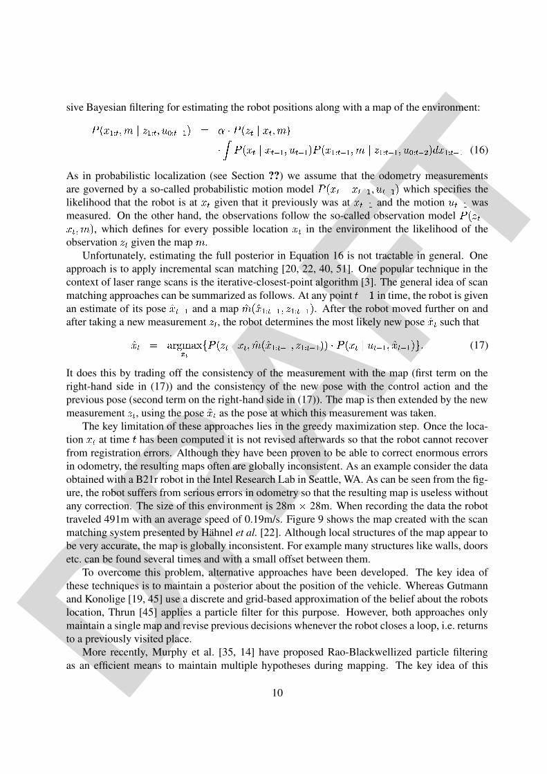
from registration errors. Although they have been proven to be able to correct enormous errorsin odometry, the resulting maps often are globally inconsistent. As an example consider the dataobtained with a B21r robot in the Intel Research Lab in Seattle, WA. As can be seen from the fig-ure, the robot suffers from serious errors in odometry so that the resulting map is useless withoutany correction. The size of this environment is 28m � 28m. When recording the data the robottraveled 491m with an average speed of 0.19m/s. Figure 9 shows the map created with the scanmatching system presented by Hahnel et al. [22]. Although local structures of the map appear tobe very accurate, the map is globally inconsistent. For example many structures like walls, doorsetc. can be found several times and with a small offset between them.

To overcome this problem, alternative approaches have been developed. The key idea ofthese techniques is to maintain a posterior about the position of the vehicle. Whereas Gutmannand Konolige [19, 45] use a discrete and grid-based approximation of the belief about the robotslocation, Thrun [45] applies a particle filter for this purpose. However, both approaches onlymaintain a single map and revise previous decisions whenever the robot closes a loop, i.e. returnsto a previously visited place.

More recently, Murphy et al. [35, 14] have proposed Rao-Blackwellized particle filteringas an efficient means to maintain multiple hypotheses during mapping. The key idea of this

10

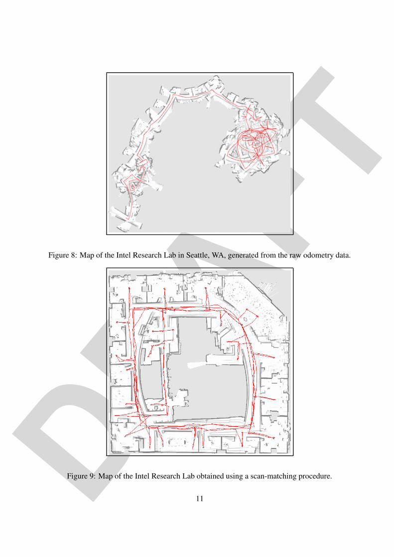
DRAFTFigure 8: Map of the Intel Research Lab in Seattle, WA, generated from the raw odometry data.

Figure 9: Map of the Intel Research Lab obtained using a scan-matching procedure.

11

DRAFT

u u

x

u

x x

z1 z2 zt

m

x 10

10 t−1

2 ... t

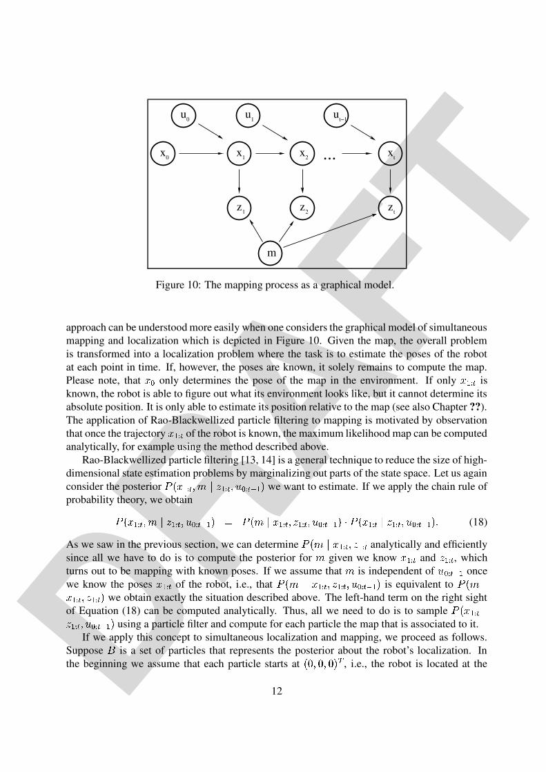
Figure 10: The mapping process as a graphical model.

approach can be understood more easily when one considers the graphical model of simultaneousmapping and localization which is depicted in Figure 10. Given the map, the overall problemis transformed into a localization problem where the task is to estimate the poses of the robotat each point in time. If, however, the poses are known, it solely remains to compute the map.Please note, that ��� only determines the pose of the map in the environment. If only ���]� � isknown, the robot is able to figure out what its environment looks like, but it cannot determine itsabsolute position. It is only able to estimate its position relative to the map (see also Chapter ??).The application of Rao-Blackwellized particle filtering to mapping is motivated by observationthat once the trajectory �T�]� � of the robot is known, the maximum likelihood map can be computedanalytically, for example using the method described above.

Rao-Blackwellized particle filtering [13, 14] is a general technique to reduce the size of high-dimensional state estimation problems by marginalizing out parts of the state space. Let us againconsider the posterior ���x�T�]� �]��� ��¡+�]� �%�V¢��V� �Y£[�w¤ we want to estimate. If we apply the chain rule ofprobability theory, we obtain

�����b�]� �%���p�+¡+�]� �%��¢l�V� �Y£[�&¤p¥ �����y�4�b�]� �%�.¡+�]� �%��¢l�V� �Y£[�&¤�¦4�����b�]� �t�+¡+�]� �%��¢l�V� �Y£[�&¤:§ (18)

As we saw in the previous section, we can determine �����h�+���]� �%�.¡+�]� � analytically and efficientlysince all we have to do is to compute the posterior for � given we know �¨�]� � and ¡+�]� � , whichturns out to be mapping with known poses. If we assume that � is independent of ¢T�V� �Y£[� oncewe know the poses �T�]� � of the robot, i.e., that ����� ���T�]� �%�.¡+�]� �%��¢l�V� �Y£[�&¤ is equivalent to ����� ��b�]� �%�.¡+�]� ��¤ we obtain exactly the situation described above. The left-hand term on the right sightof Equation (18) can be computed analytically. Thus, all we need to do is to sample ���x���]� �©�¡+�]� �%��¢l�V� �Y£[�&¤ using a particle filter and compute for each particle the map that is associated to it.

If we apply this concept to simultaneous localization and mapping, we proceed as follows.Suppose ª is a set of particles that represents the posterior about the robot’s localization. Inthe beginning we assume that each particle starts at ��«0�.«0�.«�¤&¬ , i.e., the robot is located at the

12

DRAFT

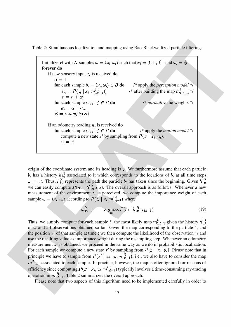
Table 2: Simultaneous localization and mapping using Rao-Blackwellized particle filtering.

Initialize ­ with ® samples ¯.°�±�²�³[°µ´&¶�°�· such that ³l°�±�¸¹@´.¹0´.¹�º¼» and ¶¨°�± ½¾forever do

if new sensory input ¿DÀ is received doÁ ±Â¹for each sample ¯.°�±�²�³[°µ´&¶�°�·ÄÃÅ­ do /* apply the perception model */Æ °}±6Ç�¸�¿sÀ�È4³[°]´VÉ�Ê °Ì˽]Í ÀYÎ ½ ºVº /* after building the map É�Ê °Ì˽]Í ÀYÎ ½ º */Á ± Á�ÏÐÆ °for each sample ²�³l°µ´&¶�°�·ÄÃÅ­ do /* normalize the weights */Æ °}± Á Î ½¨Ñ Æ °­Ò±ÒÓ�Ô.ÕsÖ�×ÙØ�ÚÛÔ�¸­Üº

if an odometry reading Ý�À is received dofor each sample ²�³l°µ´&¶�°�·ÄÃÅ­ do /* apply the motion model */

compute a new state ³lÞ by sampling from Ç�¸�³lÞEÈ4³[°]´VÝlÀxº .³[°�±Â³[Þ

origin of the coordinate system and its heading is ¹ . We furthermore assume that each particle¯�° has a history ß�Ê °Ì˽]Í À associated to it which corresponds to the locations of ¯à° at all time stepsá ´DâsâDâs´Vã . Thus, ß}Ê °Ì˽]Í À represents the path the particle ¯{° has taken since the beginning. Given ßTÊ °Ì˽]Í Àwe can easily compute Ç�¸�É ÈbßbÊ °Ì˽]Í À ´�¿ ½]Í Àº . The overall approach is as follows. Whenever a newmeasurement of the environment ¿4À is perceived, we compute the importance weight of eachsample ¯.°�±�²�³[°¼´&¶�°�· according to Ç�¸¿sÀ�È4³[°]´VÉ�Ê °Ì˽]Í ÀYÎ ½ º where

É Ê °Ì˽]Í ÀYÎ ½ ± ä�å&æ�ç�äHèé Ç�¸�ÉpÈ+ß Ê °ê˽]Í À ´.¿ ½]Í ÀYÎ ½ º (19)

Thus, we simply compute for each sample ¯{° the most likely map É Ê °ê˽]Í ÀYÎ ½ given the history ß Ê °Ì˽]Í Àof ¯�° and all observations obtained so far. Given the map corresponding to the particle ¯s° andthe position ³lÀ of that sample at time ã we then compute the likelihood of the observation ¿HÀ anduse the resulting value as importance weight during the resampling step. Whenever an odometrymeasurement ÝlÀ is obtained, we proceed in the same way as we do in probabilistic localization.For each sample we compute a new state ³�Þ by sampling from Ç�¸�³lÞ¨È+³[°¼´�Ý[À�º . Please note that inprinciple we have to sample from Ç�¸x³�ÞëÈ[³[°]´�Ý[À]´VÉ�Ê °Ì˽]Í ÀYÎ ½ º , i.e., we also have to consider the mapÉ�Ê °Ì˽]Í ÀYÎ ½ associated to each sample. In practice, however, the map is often ignored for reasons ofefficiency since computing Ç�¸�³�ÞTÈ!³[°µ´�Ý[À]´�É�Ê °Ì˽]Í ÀYÎ ½ º typically involves a time-consuming ray-tracingoperation in É Ê °Ì˽]Í ÀYÎ ½ . Table 2 summarizes the overall approach.

Please note that two aspects of this algorithm need to be implemented carefully in order to

13

DRAFT(a) (b) (c)

(d) (e) (f)

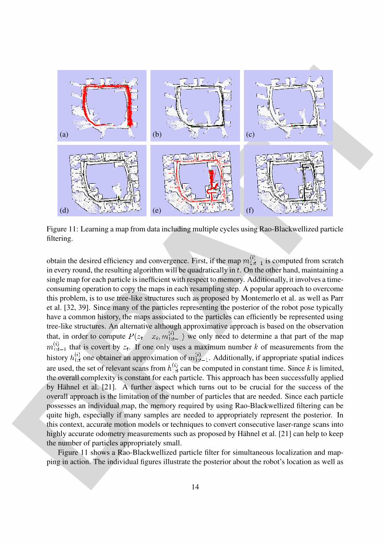
Figure 11: Learning a map from data including multiple cycles using Rao-Blackwellized particlefiltering.

obtain the desired efficiency and convergence. First, if the map ì�íBîÌïð]ñ òYó[ð is computed from scratchin every round, the resulting algorithm will be quadratically in ô . On the other hand, maintaining asingle map for each particle is inefficient with respect to memory. Additionally, it involves a time-consuming operation to copy the maps in each resampling step. A popular approach to overcomethis problem, is to use tree-like structures such as proposed by Montemerlo et al. as well as Parret al. [32, 39]. Since many of the particles representing the posterior of the robot pose typicallyhave a common history, the maps associated to the particles can efficiently be represented usingtree-like structures. An alternative although approximative approach is based on the observationthat, in order to compute õ�ö÷ ò�øTù î¼ú ì�í8îêïð]ñ òYó[ð&û we only need to determine a that part of the mapì�íBîÌïð]ñ òYó[ð that is covert by ÷ ò . If one only uses a maximum number ü of measurements from thehistory ý�íBîÌïð]ñ ò one obtainer an approximation of ìÅíBîÌïð]ñ òYó[ð . Additionally, if appropriate spatial indicesare used, the set of relevant scans from ý íBîÌïð]ñ ò can be computed in constant time. Since ü is limited,the overall complexity is constant for each particle. This approach has been successfully appliedby Hahnel et al. [21]. A further aspect which turns out to be crucial for the success of theoverall approach is the limitation of the number of particles that are needed. Since each particlepossesses an individual map, the memory required by using Rao-Blackwellized filtering can bequite high, especially if many samples are needed to appropriately represent the posterior. Inthis context, accurate motion models or techniques to convert consecutive laser-range scans intohighly accurate odometry measurements such as proposed by Hahnel et al. [21] can help to keepthe number of particles appropriately small.

Figure 11 shows a Rao-Blackwellized particle filter for simultaneous localization and map-ping in action. The individual figures illustrate the posterior about the robot’s location as well as

14

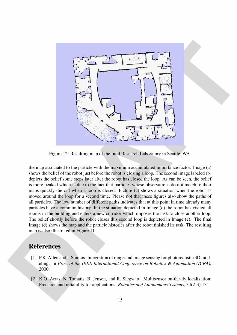
DRAFTFigure 12: Resulting map of the Intel Research Laboratory in Seattle, WA.

the map associated to the particle with the maximum accumulated importance factor. Image (a)shows the belief of the robot just before the robot is closing a loop. The second image labeled (b)depicts the belief some steps later after the robot has closed the loop. As can be seen, the beliefis more peaked which is due to the fact that particles whose observations do not match to theirmaps quickly die out when a loop is closed. Picture (c) shows a situation when the robot asmoved around the loop for a second time. Please not that these figures also show the paths ofall particles. The low number of different paths indicates that at this point in time already manyparticles have a common history. In the situation depicted in Image (d) the robot has visited allrooms in the building and enters a new corridor which imposes the task to close another loop.The belief shortly before the robot closes this second loop is depicted in Image (e). The finalImage (d) shows the map and the particle histories after the robot finished its task. The resultingmap is also illustrated in Figure 11.

References[1] P.K. Allen and I. Stamos. Integration of range and image sensing for photorealistic 3D mod-

eling. In Proc. of the IEEE International Conference on Robotics & Automation (ICRA),2000.

[2] K.O. Arras, N. Tomatis, B. Jensen, and R. Siegwart. Multisensor on-the-fly localization:Precision and reliability for applications. Robotics and Autonomous Systems, 34(2-3):131–

15

DRAFT

143, 2001.

[3] P. Besl and N. McKay. A method for registration of 3d shapes. IEEE Transactions onPattern Analysis and Machine Intelligence, 18(14):239–256, 1992.

[4] W. Burgard, A.B. Cremers, D. Fox, D. Hahnel, G. Lakemeyer, D. Schulz, W. Steiner, andS. Thrun. Experiences with an interactive museum tour-guide robot. Artificial Intelligence,114(1-2), 2000.

[5] W. Burgard, D. Fox, H. Jans, C. Matenar, and S. Thrun. Sonar-based mapping of large-scalemobile robot environments using EM. In Proc. of the International Conference on MachineLearning (ICML), 1999.

[6] J.A. Castellanos, J.M.M. Montiel, J. Neira, and J.D. Tardos. The SPmap: A probabilisticframework for simultaneous localization and map building. IEEE Transactions on Roboticsand Automation, 15(5):948–953, 1999.

[7] J.A. Castellanos and J.D. Tardos. Mobile Robot Localization and Map Building: A Multi-sensor Fusion Approach. Kluwer Academic Publishers, Boston, MA, 2000.

[8] H. Choset, I. Konuksven, and J.W. Burdick. Sensor Based Planning for a Planar RodRobot. In Proc. IEEE/SICE/RSJ Int. Conf. on Multisensor Fusion on Multisensor Fusionand Integration for Intelligent Systems, Washington, DC, 1996.

[9] J. Crowley. World modeling and position estimation for a mobile robot using ultrasoundranging. In Proc. of the IEEE International Conference on Robotics & Automation (ICRA),1989.

[10] F. Dellaert, S. Seitz, C. Thorpe, and S. Thrun. Structure from motion without correspon-dence. In Proc. of the IEEE Computer Society Conference on Computer Vision and PatternRecognition (CVPR), 2000.

[11] Dempster, Laird, and Rubin. Maximum likelihood from incomplete data via the em algo-rithm. Journal of the Royal Statistical Society, Series B, 39(1):1–38, 1977.

[12] G. Dissanayake, P. Newman, S. Clark, H.F. Durrant-Whyte, and Csorba M. A solutionto the simultaneous localisation and map building (slam) problem. IEEE Transactions onRobotics and Automation, 2001.

[13] A. Doucet. On sequential simulation-based methods for bayesian filtering. Technical report,Department of Engeneering, University of Cambridge, 1998.

[14] A. Doucet, J.F.G. de Freitas, K. Murphy, and S. Russel. Rao-Blackwellised particle filteringfor dynamic Bayesian networks. In Proc. of the Conference on Uncertainty in ArtificialIntelligence (UAI), 2000.

16

DRAFT

[15] A. Elfes. Using occupancy grids for mobile robot perception and navigation. IEEE Com-puter, pages 46–57, 1989.

[16] M.A. Fischler and R.C. Bolles. Random sample consensus: A paradigm for model fittingwith applications to image analysis and automated cartography. Communications of theACM, 24:381–395, 1981.

[17] C. Fruh and A. Zakhor. 3d model generation for cities using aerial photographs and groundlevel laser scans. In Proc. of the IEEE Computer Society Conference on Computer Visionand Pattern Recognition (CVPR), 2001.

[18] P. Grandjean and A. Robert de Saint Vincent. 3-D modeling of indoor scenes by fusion ofnoisy range and stereo data. In Proc. of the IEEE International Conference on Robotics &Automation (ICRA), 1989.

[19] J.-S. Gutmann and K. Konolige. Incremental mapping of large cyclic environments. InProc. of the IEEE Int. Symp. on Computational Intelligence in Robotics and Automation(CIRA), 1999.

[20] J.-S. Gutmann, T. Weigel, and B. Nebel. A fast, accurate, and robust method for self-localization in polygonal environments using laser-range-finders. Advanced Robotics Jour-nal, 14(8):651–668, 2001.

[21] D. Hahnel, W. Burgard, D. Fox, and S. Thrun. A highly efficient FastSLAM algorithm forgenerating cyclic maps of large-scale environments from raw laser range measurements.Submitted for publication.

[22] D. Hahnel, D. Schulz, and W. Burgard. Map building with mobile robots in populatedenvironments. In Proc. of the IEEE/RSJ International Conference on Intelligent Robotsand Systems (IROS), 2002.

[23] J. Hertzberg and F. Kirchner. Landmark-based autonomous navigation in sewerage pipes.In Proc. of the First Euromicro Workshop on Advanced Mobile Robots, 1996.

[24] L.P. Kaelbling, A.R. Cassandra, and J.A. Kurien. Acting under uncertainty: DiscreteBayesian models for mobile-robot navigation. In Proc. of the IEEE/RSJ International Con-ference on Intelligent Robots and Systems (IROS), 1996.

[25] S. King and C. Weiman. Helpmate autonomous mobile robot navigation system. In Proc. ofthe SPIE Conference on Mobile Robots, pages 190–198, 1990. Volume 2352.

[26] S. Koenig and R. Simmons. A robot navigation architecture based on partially observableMarkov decision process models. In D. Kortenkamp, R.P. Bonasso, and R. Murphy, editors,Artificial Intelligence and Mobile Robots. MIT/AAAI Press, Cambridge, MA, 1998.

[27] B. Kuipers and Y.T. Byun. A robot exploration and mapping strategy based on a semantichierarchy of spatial representations. Robotics and Autonomous Systems, 8 1991.

17

DRAFT

[28] S. Lacroix, R. Chatila, S. Fleury, M. Herrb, and T. Simeon. Autonomous navigation in out-door environment: Adaptive approach and experiment. In Proc. of the IEEE InternationalConference on Robotics & Automation (ICRA), 1994.

[29] J.J. Leonard and H.J.S. Feder. A computationally efficient method for large-scale concur-rent mapping and localization. In J. Hollerbach and D. Koditschek, editors, Proceedings ofthe Ninth International Symposium on Robotics Research, Salt Lake City, Utah, 1999.

[30] Y. Liu, R. Emery, D. Chakrabarti, W. Burgard, and S. Thrun. Using EM to learn 3D modelswith mobile robots. In Proceedings of the International Conference on Machine Learning(ICML), 2001.

[31] F. Lu and E. Milios. Globally consistent range scan alignment for environment mapp ing.Autonomous Robots, 4:333–349, 1997.

[32] M. Montemerlo, S. Thrun, D. Koller, and B. Wegbreit. FastSLAM: A factored solution tothe simultaneous localization and mapping problem. In Proc. of the National Conferenceon Artificial Intelligence (AAAI), 2002.

[33] H.P. Moravec. Robot spatial perception by stereoscopic vision and 3d evidence grids. Tech-nical Report CMU-RI-TR-96-34, Carnegie Mellon University, Robotics Institute, 1996.

[34] H.P. Moravec and A.E. Elfes. High resolution maps from wide angle sonar. In Proc. of theIEEE International Conference on Robotics & Automation (ICRA), 1985.

[35] K. Murphy. Bayesian map learning in dynamic environments. In Neural Info. Proc. Systems(NIPS), 1999.

[36] P.M. Newman, J.J. Leonard, J. Neira, and J. Tardos. Explore and return: Experimental vali-dation of real time concurrent mapping and localization. In Proc. of the IEEE InternationalConference on Robotics & Automation (ICRA), 2002.

[37] I. Nourbakhsh, J. Bobenage, S. Grange, R. Lutz, R. Meyer, and A. Soto. An affectivemobile educator with a full-time job. Artificial Intelligence, 114(1-2), 1999.

[38] I. Nourbakhsh, R. Powers, and S. Birchfield. DERVISH an office-navigating robot. AIMagazine, 16(2), 1995.

[39] R. Parr and A. Eliazar. Dp-slam: Fast, robust simultaneous localization and mapping with-out predetermined landmarks. In Proc. of the International Joint Conference on ArtificialIntelligence (IJCAI), 2003.

[40] T. Rofer. Using histogram correlation to create consistent laser scan maps. In Proc. of theIEEE/RSJ International Conference on Intelligent Robots and Systems (IROS), 2002.

[41] H. Samet. Applications of Spatial Data Structures. Addison-Wesley Publishing Company,1990.

18

DRAFT

[42] H Shatkay and L. Kaelbling. Learning topological maps with weak local odometric infor-mation. In Proc. of the International Joint Conference on Artificial Intelligence (IJCAI),1997.

[43] R. Simmons, R. Goodwin, K. Haigh, S. Koenig, and J. O’Sullivan. A layered architecturefor office delivery robots. In Proc. of the First International Conference on AutonomousAgents (Agents), 1997.

[44] S. Thrun. Exploration and model building in mobile robot domains. In Proc. of the IEEEInternational Conference on Neural Networks, 1993.

[45] S. Thrun. A probabilistic online mapping algorithm for teams of mobile robots. Interna-tional Journal of Robotics Research, 20(5):335–363, 2001.

[46] S. Thrun. Learning occupancy grids with forward sensor models. Autonomous Robots,2002.

[47] S. Thrun, M. Bennewitz, W. Burgard, A.B. Cremers, F. Dellaert, D. Fox, D. Hahnel,C. Rosenberg, N. Roy, J. Schulte, and D. Schulz. MINERVA: A second generation mobiletour-guide robot. In Proc. of the IEEE International Conference on Robotics & Automation(ICRA), 1999.

[48] S. Thrun, W. Burgard, and D. Fox. A real-time algorithm for mobile robot mapping withapplications to multi-robot and 3d mapping. In Proc. of the IEEE International Conferenceon Robotics & Automation (ICRA), 2000.

[49] S. Thrun, D. Fox, and W. Burgard. A probabilistic approach to concurrent mapping andlocalization for mobile robots. Machine Learning and Autonomous Robots (joint issue),31(1-3):29–53, 1998.

[50] S. Thrun, J.-S. Gutmann, D. Fox, W. Burgard, and B. Kuipers. Integrating topological andmetric maps for mobile robot navigation: A statistical approach. In Proc. of the NationalConference on Artificial Intelligence (AAAI), 1998.

[51] G. Weiß, C. Wetzler, and E. von Puttkamer. Keeping track of position and orientation ofmoving indoor systems by correlation of range-finder scans. In Proc. of the IEEE/RSJInternational Conference on Intelligent Robots and Systems (IROS), pages 595–601, 1994.

19