Drag Prediction of NASA Common Research Models Using Different Turbulence Models

Pan Du1 and Ramesh K. Agarwal2 Washington University in St. Louis, St. Louis, MO 63130

In response to the 4th and 6th AIAA Drag Prediction Workshops, this paper focuses on drag prediction of Wing-body-tail (WBT) and Wing-body-nacelle-pylon (WBNP) configurations from NASA Common Research Models. Using the ANSYS FLUENT solver, computations of the flow fields of WBT and WBNP models are performed by solving the compressible Reynolds-Averaged Navier-Stokes (RANS) equations with Spalart-Allmaras (SA) and SST k-ω turbulence models. Drag polar and drag rise curves are obtained by performing computations at different angles of attack at a constant Mach number. Pressure distributions and flow separation analyses are presented at different angles of attack. Comparison of computational results using the two turbulence models with the experimental data is provided.

Nomenclature

AR = wing aspect ratio ΑoA = angle of attack b = wing span CD = drag coefficient CP = pressure coefficient CL = lift coefficient M = Mach number Re = Reynolds number k = life curve slope em = maximum error

I. Introduction A great deal of effort has been devoted over past several decades to obtain the accurate numerical solution of flow over transonic commercial aircrafts and other aerospace industry relevant configurations using the tools of Computational Fluid Dynamics. The accurate prediction of drag has been the most challenging among all other aerodynamic coefficients. There has been rapid progress in the improvement of CFD tools namely the geometry modeling, grid generation, numerical algorithms and turbulence modeling for the accurate and efficient solution of Reynolds-Averaged Navier-Stokes (RANS) equations for the flow field of almost complete aircraft configurations; however the turbulence modeling remains a challenging task which has major influence on the accuracy of drag prediction because of relatively small magnitude of drag coefficient compared to lift coefficient. Nevertheless, at present the accuracy of cruise drag prediction of an aircraft from CFD is claimed to be within 1% range of the theoretical solution [1]. Since 2001, a series of drag prediction workshops have been organized by the AIAA Applied Aerodynamics Technical Committee [2]. The main purpose of the workshops has been to access the state-of-the art computational technology as a tool for drag, lift and moment prediction of aircrafts. The Drag Prediction Workshop (DPW) has established a platform for aerodynamics researchers from academia, industry and government labs to communicate, exchange ideas and compare results by using different meshes, turbulence models as well as flow solvers. There are many CFD solvers that have been developed worldwide by the commercial CFD vendors (e.g. ANSYS FLUENT, CFD++, CFX, STAR-CD, COMSOL etc.), and by the industry (e.g. Boeing BCFD, German Tau etc.) and the government labs (e.g. FUN3D, OVERFLOW, CFL3D, TLNS3D, COBALT, WIND etc.), and the open source software OpenFOAM that differ in mesh generation capability and numerical algorithms and in the available

1 Graduate student, Dept. of Mechanical Engineering & Materials Science, Student Member AIAA. 2 William Palm Professor of Engineering, Dept. of Mechanical Engineering & Materials Science, Fellow AIAA

1 American Institute of Aeronautics and Astronautics

Dow

nloa

ded

by N

ASA

LA

NG

LE

Y R

ESE

AR

CH

CE

NT

RE

on

Janu

ary

30, 2

018

| http

://ar

c.ai

aa.o

rg |

DO

I: 1

0.25

14/6

.201

7-42

33

35th AIAA Applied Aerodynamics Conference

5-9 June 2017, Denver, Colorado

10.2514/6.2017-4233

Copyright © 2017 by Pan Du and Ramesh K.

Agarwal. Published by the American Institute of Aeronautics and Astronautics, Inc., with permission.

AIAA AVIATION Forum

suite of turbulence models. This list is not inclusive of all the solvers that are currently in use in the CFD community. Many of these solvers have been used in solving the flow field of NASA research models identified in DPW4 and DPW6. It has been pointed out by many investigators that a turbulence model plays an important role especially in drag prediction considering other numerical aspects of various codes such as mesh generation and numerical algorithms being almost similar. Mavriplis and Long used the NSU3D solver from NASA using both the SA and standard k-ω turbulence models and found that their results are in close agreement with the collection of other results from the 4th Drag Prediction Workshop [3]. Sclafani and DeHaan employed the CFL3D solver with SA turbulence model and OVERFLOW solver with both SA and SST k-ω models to study the downwash as well as the drag polar of NASA common research model. They showed that the two equations SST k-ω model predicts a stronger shock on the wing than the one equation SA model [4].

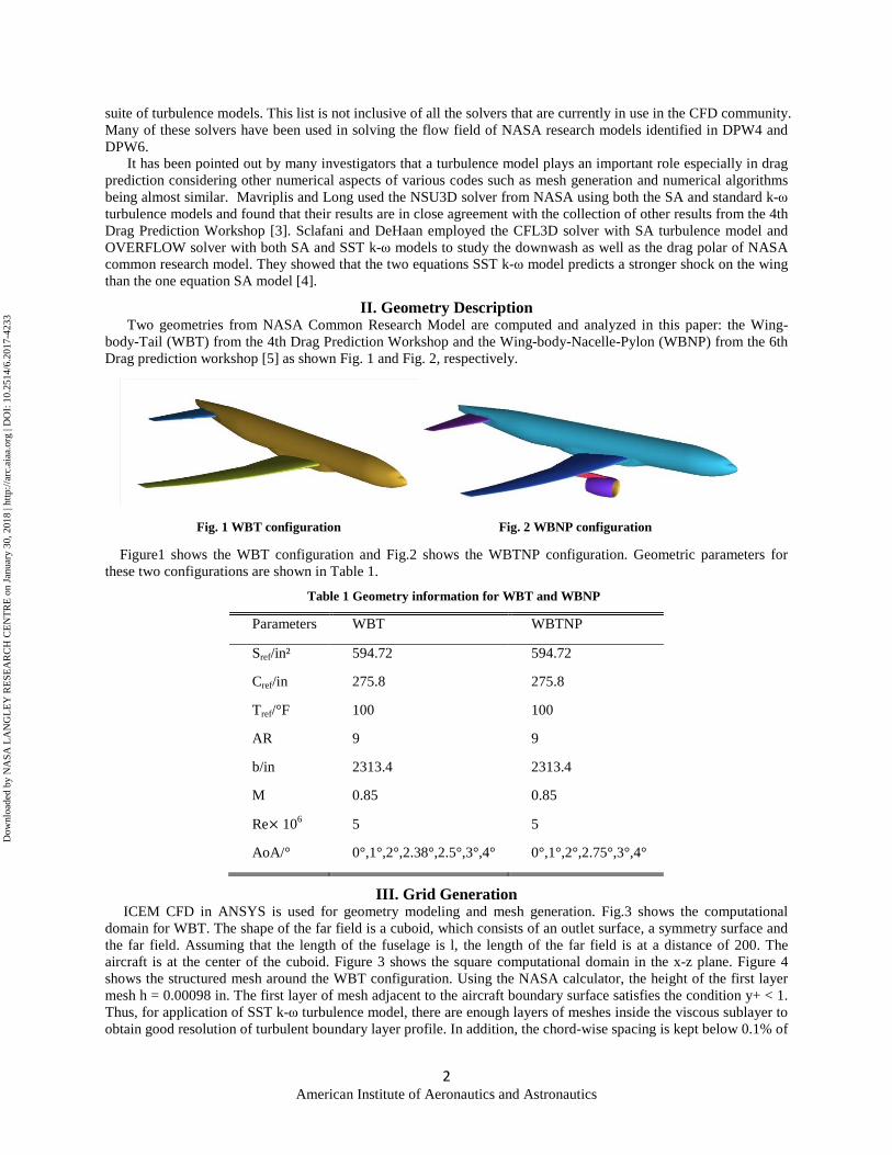
II. Geometry Description Two geometries from NASA Common Research Model are computed and analyzed in this paper: the Wing-

body-Tail (WBT) from the 4th Drag Prediction Workshop and the Wing-body-Nacelle-Pylon (WBNP) from the 6th Drag prediction workshop [5] as shown Fig. 1 and Fig. 2, respectively.

Fig. 1 WBT configuration Fig. 2 WBNP configuration

Figure1 shows the WBT configuration and Fig.2 shows the WBTNP configuration. Geometric parameters for these two configurations are shown in Table 1.

Table 1 Geometry information for WBT and WBNP

Parameters WBT WBTNP

Sref/in² 594.72 594.72

Cref/in 275.8 275.8

Tref/°F 100 100

AR 9 9

b/in 2313.4 2313.4

M 0.85 0.85

Re× 106 5 5

AoA/° 0°,1°,2°,2.38°,2.5°,3°,4° 0°,1°,2°,2.75°,3°,4°

III. Grid Generation ICEM CFD in ANSYS is used for geometry modeling and mesh generation. Fig.3 shows the computational

domain for WBT. The shape of the far field is a cuboid, which consists of an outlet surface, a symmetry surface and the far field. Assuming that the length of the fuselage is l, the length of the far field is at a distance of 200. The aircraft is at the center of the cuboid. Figure 3 shows the square computational domain in the x-z plane. Figure 4 shows the structured mesh around the WBT configuration. Using the NASA calculator, the height of the first layer mesh h = 0.00098 in. The first layer of mesh adjacent to the aircraft boundary surface satisfies the condition y+ < 1. Thus, for application of SST k-ω turbulence model, there are enough layers of meshes inside the viscous sublayer to obtain good resolution of turbulent boundary layer profile. In addition, the chord-wise spacing is kept below 0.1% of

2 American Institute of Aeronautics and Astronautics

Dow

nloa

ded

by N

ASA

LA

NG

LE

Y R

ESE

AR

CH

CE

NT

RE

on

Janu

ary

30, 2

018

| http

://ar

c.ai

aa.o

rg |

DO

I: 1

0.25

14/6

.201

7-42

33

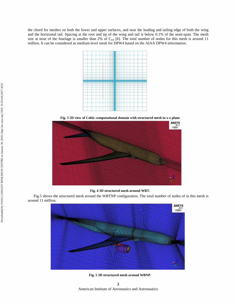
the chord for meshes on both the lower and upper surfaces, and near the leading and tailing edge of both the wing and the horizontal tail. Spacing at the root and tip of the wing and tail is below 0.1% of the semi-span. The mesh size at nose of the fuselage is smaller than 2% of Cref [6]. The total number of nodes for this mesh is around 11 million. It can be considered as medium level mesh for DPW4 based on the AIAA DPW4 information.

Fig. 3 2D view of Cubic computational domain with structured mesh in x-z plane

Fig. 4 3D structured mesh around WBT. Fig.5 shows the structured mesh around the WBTNP configuration. The total number of nodes of in this mesh is around 11 million.

Fig. 5 3D structured mesh around WBNP.

3 American Institute of Aeronautics and Astronautics

Dow

nloa

ded

by N

ASA

LA

NG

LE

Y R

ESE

AR

CH

CE

NT

RE

on

Janu

ary

30, 2

018

| http

://ar

c.ai

aa.o

rg |

DO

I: 1

0.25

14/6

.201

7-42

33

IV. Results and Discussion A. Analysis of WBT from DPW4

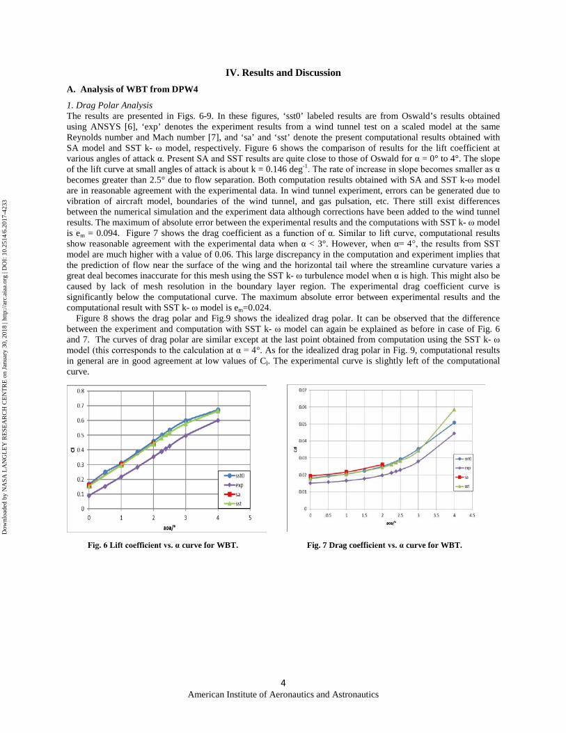
1. Drag Polar Analysis The results are presented in Figs. 6-9. In these figures, ‘sst0’ labeled results are from Oswald’s results obtained using ANSYS [6], ‘exp’ denotes the experiment results from a wind tunnel test on a scaled model at the same Reynolds number and Mach number [7], and ‘sa’ and ‘sst’ denote the present computational results obtained with SA model and SST k- ω model, respectively. Figure 6 shows the comparison of results for the lift coefficient at various angles of attack α. Present SA and SST results are quite close to those of Oswald for α = 0° to 4°. The slope of the lift curve at small angles of attack is about k = 0.146 deg-1. The rate of increase in slope becomes smaller as α becomes greater than 2.5° due to flow separation. Both computation results obtained with SA and SST k-ω model are in reasonable agreement with the experimental data. In wind tunnel experiment, errors can be generated due to vibration of aircraft model, boundaries of the wind tunnel, and gas pulsation, etc. There still exist differences between the numerical simulation and the experiment data although corrections have been added to the wind tunnel results. The maximum of absolute error between the experimental results and the computations with SST k- ω model is em = 0.094. Figure 7 shows the drag coefficient as a function of α. Similar to lift curve, computational results show reasonable agreement with the experimental data when α < 3°. However, when α= 4°, the results from SST model are much higher with a value of 0.06. This large discrepancy in the computation and experiment implies that the prediction of flow near the surface of the wing and the horizontal tail where the streamline curvature varies a great deal becomes inaccurate for this mesh using the SST k- ω turbulence model when α is high. This might also be caused by lack of mesh resolution in the boundary layer region. The experimental drag coefficient curve is significantly below the computational curve. The maximum absolute error between experimental results and the computational result with SST k- ω model is em=0.024. Figure 8 shows the drag polar and Fig.9 shows the idealized drag polar. It can be observed that the difference between the experiment and computation with SST k- ω model can again be explained as before in case of Fig. 6 and 7. The curves of drag polar are similar except at the last point obtained from computation using the SST k- ω model (this corresponds to the calculation at α = 4°. As for the idealized drag polar in Fig. 9, computational results in general are in good agreement at low values of Cl. The experimental curve is slightly left of the computational curve.

Fig. 6 Lift coefficient vs. α curve for WBT. Fig. 7 Drag coefficient vs. α curve for WBT.

4 American Institute of Aeronautics and Astronautics

Dow

nloa

ded

by N

ASA

LA

NG

LE

Y R

ESE

AR

CH

CE

NT

RE

on

Janu

ary

30, 2

018

| http

://ar

c.ai

aa.o

rg |

DO

I: 1

0.25

14/6

.201

7-42

33

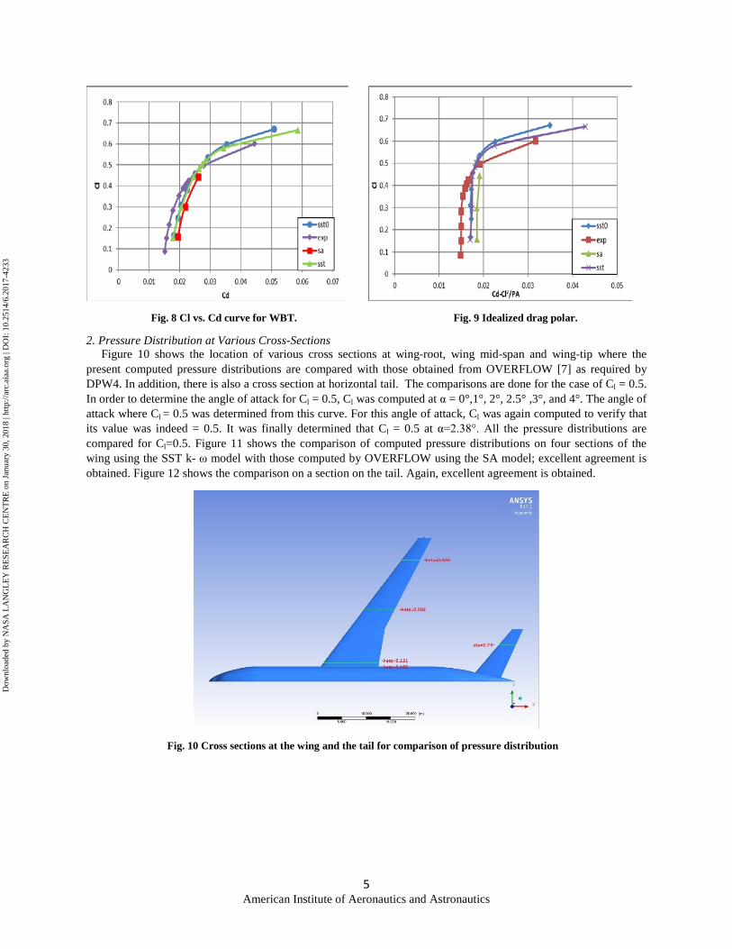
Fig. 8 Cl vs. Cd curve for WBT. Fig. 9 Idealized drag polar.

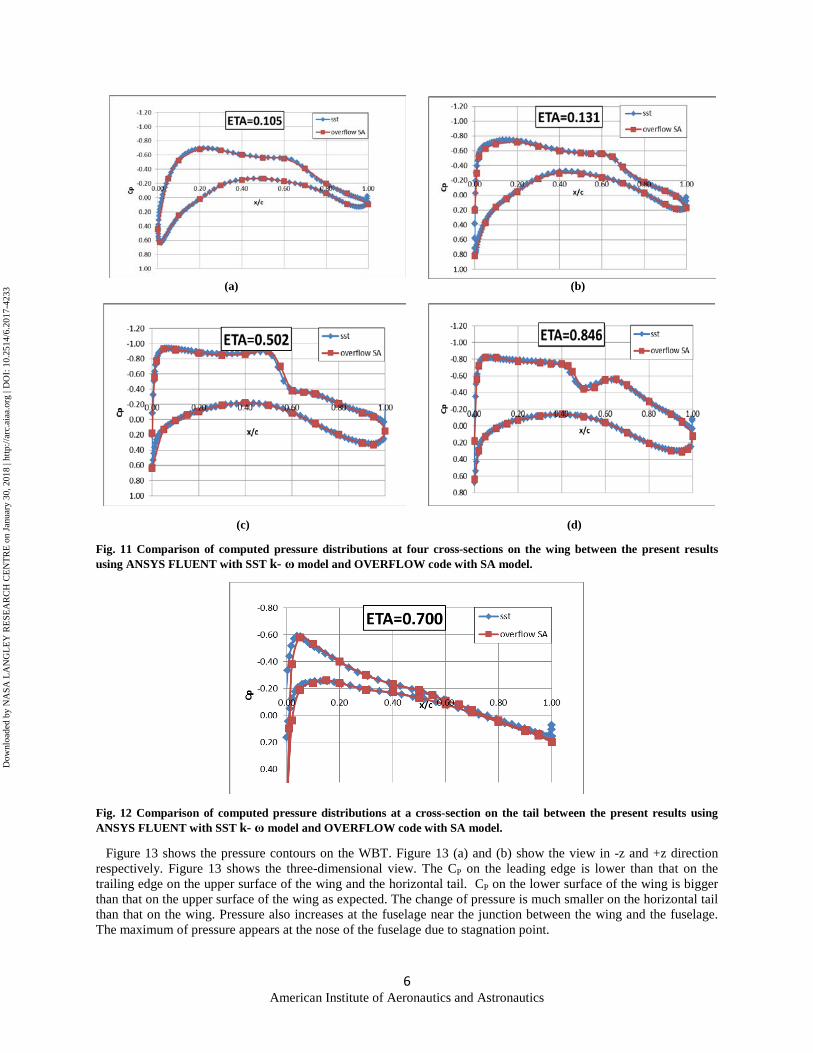
2. Pressure Distribution at Various Cross-Sections Figure 10 shows the location of various cross sections at wing-root, wing mid-span and wing-tip where the present computed pressure distributions are compared with those obtained from OVERFLOW [7] as required by DPW4. In addition, there is also a cross section at horizontal tail. The comparisons are done for the case of Cl = 0.5. In order to determine the angle of attack for Cl = 0.5, Cl was computed at α = 0°,1°, 2°, 2.5° ,3°, and 4°. The angle of attack where Cl = 0.5 was determined from this curve. For this angle of attack, Cl was again computed to verify that its value was indeed = 0.5. It was finally determined that Cl = 0.5 at α=2.38°. All the pressure distributions are compared for Cl=0.5. Figure 11 shows the comparison of computed pressure distributions on four sections of the wing using the SST k- ω model with those computed by OVERFLOW using the SA model; excellent agreement is obtained. Figure 12 shows the comparison on a section on the tail. Again, excellent agreement is obtained.

Fig. 10 Cross sections at the wing and the tail for comparison of pressure distribution

5 American Institute of Aeronautics and Astronautics

Dow

nloa

ded

by N

ASA

LA

NG

LE

Y R

ESE

AR

CH

CE

NT

RE

on

Janu

ary

30, 2

018

| http

://ar

c.ai

aa.o

rg |

DO

I: 1

0.25

14/6

.201

7-42

33

(a) (b)

(c) (d)

Fig. 11 Comparison of computed pressure distributions at four cross-sections on the wing between the present results using ANSYS FLUENT with SST k- ω model and OVERFLOW code with SA model.

Fig. 12 Comparison of computed pressure distributions at a cross-section on the tail between the present results using ANSYS FLUENT with SST k- ω model and OVERFLOW code with SA model.

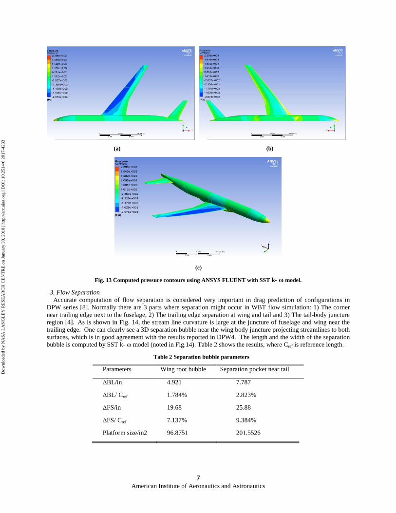
Figure 13 shows the pressure contours on the WBT. Figure 13 (a) and (b) show the view in -z and +z direction respectively. Figure 13 shows the three-dimensional view. The CP on the leading edge is lower than that on the trailing edge on the upper surface of the wing and the horizontal tail. CP on the lower surface of the wing is bigger than that on the upper surface of the wing as expected. The change of pressure is much smaller on the horizontal tail than that on the wing. Pressure also increases at the fuselage near the junction between the wing and the fuselage. The maximum of pressure appears at the nose of the fuselage due to stagnation point.

6 American Institute of Aeronautics and Astronautics

Dow

nloa

ded

by N

ASA

LA

NG

LE

Y R

ESE

AR

CH

CE

NT

RE

on

Janu

ary

30, 2

018

| http

://ar

c.ai

aa.o

rg |

DO

I: 1

0.25

14/6

.201

7-42

33

(a) (b)

(c)

Fig. 13 Computed pressure contours using ANSYS FLUENT with SST k- ω model.

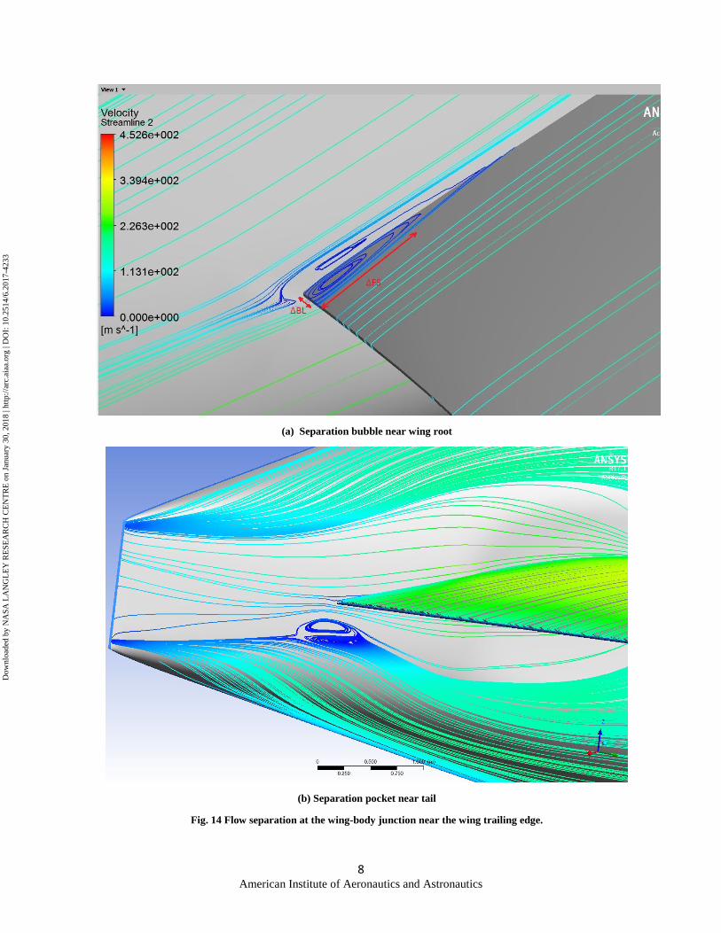
3. Flow Separation Accurate computation of flow separation is considered very important in drag prediction of configurations in

DPW series [8]. Normally there are 3 parts where separation might occur in WBT flow simulation: 1) The corner near trailing edge next to the fuselage, 2) The trailing edge separation at wing and tail and 3) The tail-body juncture region [4]. As is shown in Fig. 14, the stream line curvature is large at the juncture of fuselage and wing near the trailing edge. One can clearly see a 3D separation bubble near the wing body juncture projecting streamlines to both surfaces, which is in good agreement with the results reported in DPW4. The length and the width of the separation bubble is computed by SST k- ω model (noted in Fig.14). Table 2 shows the results, where Cref is reference length.

Table 2 Separation bubble parameters

Parameters Wing root bubble Separation pocket near tail

ΔBL/in 4.921 7.787

ΔBL/ Cref 1.784% 2.823%

ΔFS/in 19.68 25.88

ΔFS/ Cref 7.137% 9.384%

Platform size/in2 96.8751 201.5526

7 American Institute of Aeronautics and Astronautics

Dow

nloa

ded

by N

ASA

LA

NG

LE

Y R

ESE

AR

CH

CE

NT

RE

on

Janu

ary

30, 2

018

| http

://ar

c.ai

aa.o

rg |

DO

I: 1

0.25

14/6

.201

7-42

33

(a) Separation bubble near wing root

(b) Separation pocket near tail

Fig. 14 Flow separation at the wing-body junction near the wing trailing edge.

8 American Institute of Aeronautics and Astronautics

Dow

nloa

ded

by N

ASA

LA

NG

LE

Y R

ESE

AR

CH

CE

NT

RE

on

Janu

ary

30, 2

018

| http

://ar

c.ai

aa.o

rg |

DO

I: 1

0.25

14/6

.201

7-42

33

From Table 2, bubble length and width is 7.137% and 1.784% of the reference length respectively. It is within reasonable range of percentage error for the size of separation bubble. There exists separation near the wing fuselage juncture when angle of attack is 2.38°. As shown in Fig.14, the separation pocket is well defined by the solution on 10 million grid points. The results show that the platform size of the pocket is bigger than the separation bubble at the wing root.

B. Analysis of WBPN from DPW6

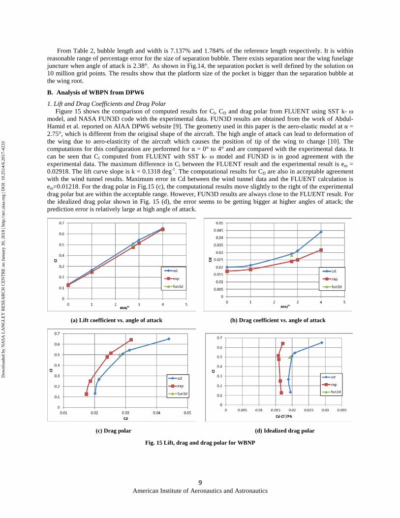
1. Lift and Drag Coefficients and Drag Polar Figure 15 shows the comparison of computed results for Cl, CD and drag polar from FLUENT using SST k- ω model, and NASA FUN3D code with the experimental data. FUN3D results are obtained from the work of Abdul-Hamid et al. reported on AIAA DPW6 website [9]. The geometry used in this paper is the aero-elastic model at α = 2.75°, which is different from the original shape of the aircraft. The high angle of attack can lead to deformation of the wing due to aero-elasticity of the aircraft which causes the position of tip of the wing to change [10]. The computations for this configuration are performed for α = 0° to 4° and are compared with the experimental data. It can be seen that Cl computed from FLUENT with SST k- ω model and FUN3D is in good agreement with the experimental data. The maximum difference in Cl between the FLUENT result and the experimental result is em = 0.02918. The lift curve slope is k = 0.1318 deg-1. The computational results for CD are also in acceptable agreement with the wind tunnel results. Maximum error in Cd between the wind tunnel data and the FLUENT calculation is em=0.01218. For the drag polar in Fig.15 (c), the computational results move slightly to the right of the experimental drag polar but are within the acceptable range. However, FUN3D results are always close to the FLUENT result. For the idealized drag polar shown in Fig. 15 (d), the error seems to be getting bigger at higher angles of attack; the prediction error is relatively large at high angle of attack.

(a) Lift coefficient vs. angle of attack (b) Drag coefficient vs. angle of attack

(c) Drag polar (d) Idealized drag polar

Fig. 15 Lift, drag and drag polar for WBNP

9 American Institute of Aeronautics and Astronautics

Dow

nloa

ded

by N

ASA

LA

NG

LE

Y R

ESE

AR

CH

CE

NT

RE

on

Janu

ary

30, 2

018

| http

://ar

c.ai

aa.o

rg |

DO

I: 1

0.25

14/6

.201

7-42

33

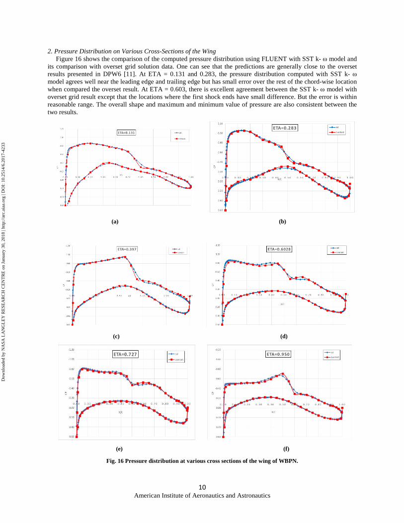
2. Pressure Distribution on Various Cross-Sections of the Wing Figure 16 shows the comparison of the computed pressure distribution using FLUENT with SST k- ω model and its comparison with overset grid solution data. One can see that the predictions are generally close to the overset results presented in DPW6 [11]. At ETA = 0.131 and 0.283, the pressure distribution computed with SST k- ω model agrees well near the leading edge and trailing edge but has small error over the rest of the chord-wise location when compared the overset result. At ETA = 0.603, there is excellent agreement between the SST k- ω model with overset grid result except that the locations where the first shock ends have small difference. But the error is within reasonable range. The overall shape and maximum and minimum value of pressure are also consistent between the two results.

(a) (b)

(c) (d)

(e) (f)

Fig. 16 Pressure distribution at various cross sections of the wing of WBPN.

10 American Institute of Aeronautics and Astronautics

Dow

nloa

ded

by N

ASA

LA

NG

LE

Y R

ESE

AR

CH

CE

NT

RE

on

Janu

ary

30, 2

018

| http

://ar

c.ai

aa.o

rg |

DO

I: 1

0.25

14/6

.201

7-42

33

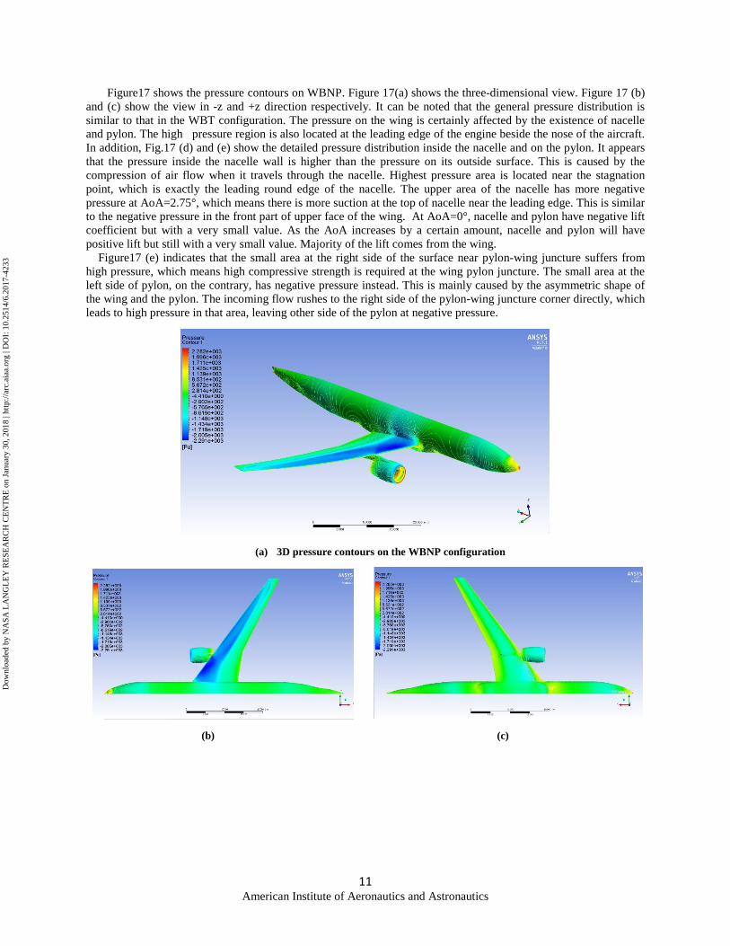
Figure17 shows the pressure contours on WBNP. Figure 17(a) shows the three-dimensional view. Figure 17 (b) and (c) show the view in -z and +z direction respectively. It can be noted that the general pressure distribution is similar to that in the WBT configuration. The pressure on the wing is certainly affected by the existence of nacelle and pylon. The high pressure region is also located at the leading edge of the engine beside the nose of the aircraft. In addition, Fig.17 (d) and (e) show the detailed pressure distribution inside the nacelle and on the pylon. It appears that the pressure inside the nacelle wall is higher than the pressure on its outside surface. This is caused by the compression of air flow when it travels through the nacelle. Highest pressure area is located near the stagnation point, which is exactly the leading round edge of the nacelle. The upper area of the nacelle has more negative pressure at AoA=2.75°, which means there is more suction at the top of nacelle near the leading edge. This is similar to the negative pressure in the front part of upper face of the wing. At AoA=0°, nacelle and pylon have negative lift coefficient but with a very small value. As the AoA increases by a certain amount, nacelle and pylon will have positive lift but still with a very small value. Majority of the lift comes from the wing.

Figure17 (e) indicates that the small area at the right side of the surface near pylon-wing juncture suffers from high pressure, which means high compressive strength is required at the wing pylon juncture. The small area at the left side of pylon, on the contrary, has negative pressure instead. This is mainly caused by the asymmetric shape of the wing and the pylon. The incoming flow rushes to the right side of the pylon-wing juncture corner directly, which leads to high pressure in that area, leaving other side of the pylon at negative pressure.

(a) 3D pressure contours on the WBNP configuration

(b) (c)

11 American Institute of Aeronautics and Astronautics

Dow

nloa

ded

by N

ASA

LA

NG

LE

Y R

ESE

AR

CH

CE

NT

RE

on

Janu

ary

30, 2

018

| http

://ar

c.ai

aa.o

rg |

DO

I: 1

0.25

14/6

.201

7-42

33

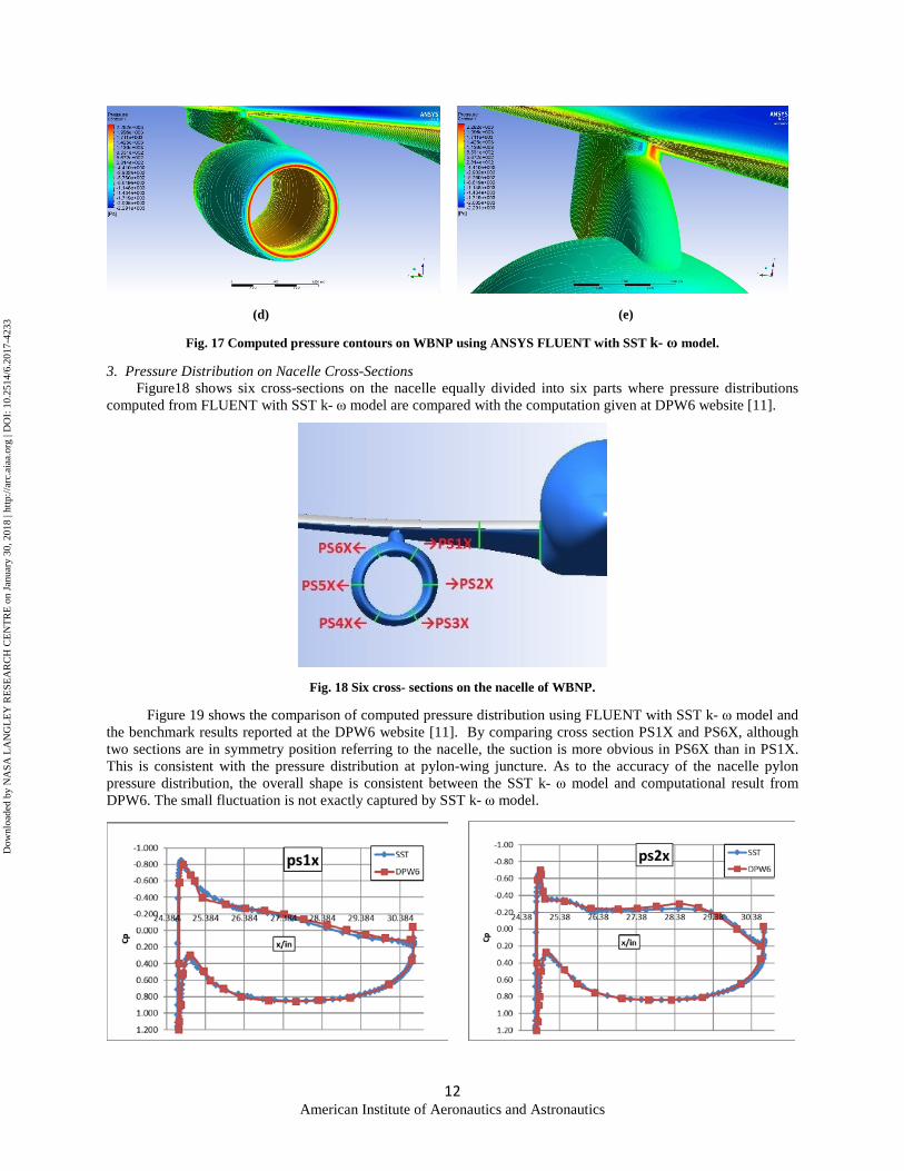
(d) (e)

Fig. 17 Computed pressure contours on WBNP using ANSYS FLUENT with SST k- ω model.

3. Pressure Distribution on Nacelle Cross-Sections Figure18 shows six cross-sections on the nacelle equally divided into six parts where pressure distributions

computed from FLUENT with SST k- ω model are compared with the computation given at DPW6 website [11].

Fig. 18 Six cross- sections on the nacelle of WBNP.

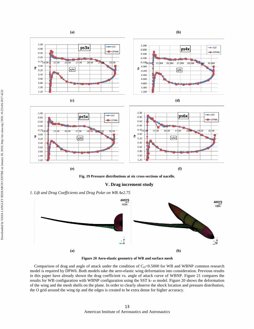
Figure 19 shows the comparison of computed pressure distribution using FLUENT with SST k- ω model and the benchmark results reported at the DPW6 website [11]. By comparing cross section PS1X and PS6X, although two sections are in symmetry position referring to the nacelle, the suction is more obvious in PS6X than in PS1X. This is consistent with the pressure distribution at pylon-wing juncture. As to the accuracy of the nacelle pylon pressure distribution, the overall shape is consistent between the SST k- ω model and computational result from DPW6. The small fluctuation is not exactly captured by SST k- ω model.

12 American Institute of Aeronautics and Astronautics

Dow

nloa

ded

by N

ASA

LA

NG

LE

Y R

ESE

AR

CH

CE

NT

RE

on

Janu

ary

30, 2

018

| http

://ar

c.ai

aa.o

rg |

DO

I: 1

0.25

14/6

.201

7-42

33

(a) (b)

(c) (d)

(e) (f)

Fig. 19 Pressure distributions at six cross-sections of nacelle.

V. Drag increment study

1. Lift and Drag Coefficients and Drag Polar on WB Ae2.75

(a) (b)

Figure 20 Aero-elastic geometry of WB and surface mesh

Comparison of drag and angle of attack under the condition of CD=0.5000 for WB and WBNP common research model is required by DPW6. Both models take the aero-elastic wing deformation into consideration. Previous results in this paper have already shown the drag coefficient vs. angle of attack curve of WBNP. Figure 21 compares the results for WB configuration with WBNP configuration using the SST k- ω model. Figure 20 shows the deformation of the wing and the mesh shells on the plane. In order to clearly observe the shock location and pressure distribution, the O grid around the wing tip and the edges is created to be extra dense for higher accuracy.

13 American Institute of Aeronautics and Astronautics

Dow

nloa

ded

by N

ASA

LA

NG

LE

Y R

ESE

AR

CH

CE

NT

RE

on

Janu

ary

30, 2

018

| http

://ar

c.ai

aa.o

rg |

DO

I: 1

0.25

14/6

.201

7-42

33

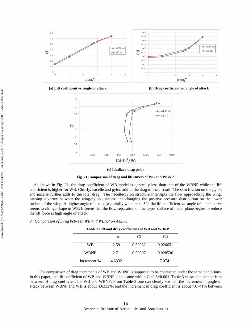
(a) Lift coefficient vs. angle of attack (b) Drag coefficient vs. angle of attack

(c) Idealized drag polar

Fig. 21 Comparison of drag and lift curves of WB and WBNP.

As shown in Fig. 21, the drag coefficient of WB model is generally less than that of the WBNP while the lift coefficient is higher for WB. Clearly, nacelle and pylon add to the drag of the aircraft. The skin friction on the pylon and nacelle further adds to the total drag. The nacelle-pylon structure interrupts the flow approaching the wing, causing a vortex between the wing-pylon juncture and changing the positive pressure distribution on the lower surface of the wing. At higher angle of attack (especially when α >= 3°), the lift coefficient vs. angle of attack curve seems to change shape in WB. It seems that the flow separation on the upper surface of the airplane begins to reduce the lift force at high angle of attack.

2. Comparison of Drag between WB and WBNP on Ae2.75

Table 3 Lift and drag coefficients of WB and WBNP

α Cl Cd

WB 2.59 0.50032 0.026651

WBNP 2.71 0.50097 0.028536

Increment % 4.6332

7.0741

The comparison of drag increments of WB and WBNP is supposed to be conducted under the same conditions. In this paper, the lift coefficient of WB and WBNP is the same within Cl=0.5±0.001. Table 3 shows the comparison between of drag coefficient for WB and WBNP. From Table 3 one can clearly see that the increment in angle of attack between WBNP and WB is about 4.6332%, and the increment in drag coefficient is about 7.0741% between

14 American Institute of Aeronautics and Astronautics

Dow

nloa

ded

by N

ASA

LA

NG

LE

Y R

ESE

AR

CH

CE

NT

RE

on

Janu

ary

30, 2

018

| http

://ar

c.ai

aa.o

rg |

DO

I: 1

0.25

14/6

.201

7-42

33

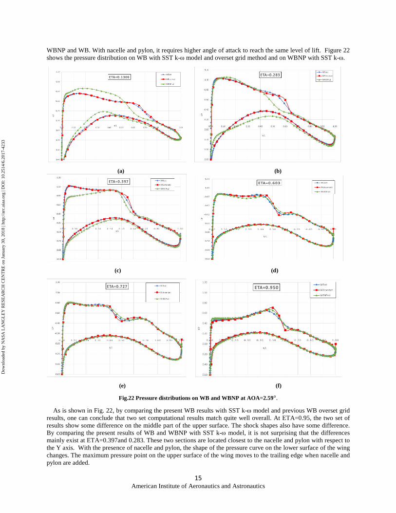
WBNP and WB. With nacelle and pylon, it requires higher angle of attack to reach the same level of lift. Figure 22 shows the pressure distribution on WB with SST k-ω model and overset grid method and on WBNP with SST k-ω.

(a) (b)

(c) (d)

(e) (f)

Fig.22 Pressure distributions on WB and WBNP at AOA=2.59°.

As is shown in Fig. 22, by comparing the present WB results with SST k-ω model and previous WB overset grid results, one can conclude that two set computational results match quite well overall. At ETA=0.95, the two set of results show some difference on the middle part of the upper surface. The shock shapes also have some difference. By comparing the present results of WB and WBNP with SST k-ω model, it is not surprising that the differences mainly exist at ETA=0.397and 0.283. These two sections are located closest to the nacelle and pylon with respect to the Y axis. With the presence of nacelle and pylon, the shape of the pressure curve on the lower surface of the wing changes. The maximum pressure point on the upper surface of the wing moves to the trailing edge when nacelle and pylon are added.

15 American Institute of Aeronautics and Astronautics

Dow

nloa

ded

by N

ASA

LA

NG

LE

Y R

ESE

AR

CH

CE

NT

RE

on

Janu

ary

30, 2

018

| http

://ar

c.ai

aa.o

rg |

DO

I: 1

0.25

14/6

.201

7-42

33

3. Separated flow at Wing-Body Configuration at Angle Sweep.

(a) AoA=2.75° (b) AoA=3.00°

(c) AoA=3.5° (d) AoA=4°

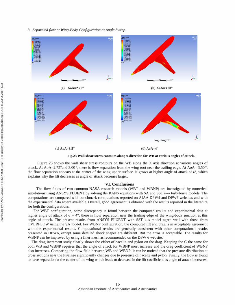
Fig.23 Wall shear stress contours along x-direction for WB at various angles of attack.

Figure 23 shows the wall shear stress contours on the WB along the X axis direction at various angles of attack. At AoA=2.75°and 3.00 °, there is flow separation from the wing root near the trailing edge. At AoA= 3.50 °, the flow separation appears at the center of the wing upper surface. It grows at higher angle of attack of 4°, which explains why the lift decreases as angle of attack becomes larger.

VI. Conclusions The flow fields of two common NASA research models (WBT and WBNP) are investigated by numerical

simulations using ANSYS FLUENT by solving the RANS equations with SA and SST k-ω turbulence models. The computations are compared with benchmark computations reported on AIAA DPW4 and DPW6 websites and with the experimental data where available. Overall, good agreement is obtained with the results reported in the literature for both the configurations.

For WBT configuration, some discrepancy is found between the computed results and experimental data at higher angle of attack of α = 4°; there is flow separation near the trailing edge of the wing-body junction at this angle of attack. The present results from ANSYS FLUENT with SST k-ω model agree well with those from OVERFLOW using the SA model. For WBNP configuration, the computed lift and drag is in acceptable agreement with the experimental results. Computational results are generally consistent with other computational results presented in DPW6, except some detailed shock shapes are different. But the error is acceptable. The results for WBNP can be improved by using a finer mesh as recommended on the DPW 6 website.

The drag increment study clearly shows the effect of nacelle and pylon on the drag. Keeping the Cl the same for both WB and WBNP requires that the angle of attack for WBNP must increase and the drag coefficient of WBNP also increases. Comparing the flow field between WB and WBNP, it can be noticed that the pressure distribution at cross sections near the fuselage significantly changes due to presence of nacelle and pylon. Finally, the flow is found to have separation at the center of the wing which leads to decrease in the lift coefficient as angle of attack increases.

16 American Institute of Aeronautics and Astronautics

Dow

nloa

ded

by N

ASA

LA

NG

LE

Y R

ESE

AR

CH

CE

NT

RE

on

Janu

ary

30, 2

018

| http

://ar

c.ai

aa.o

rg |

DO

I: 1

0.25

14/6

.201

7-42

33

References

[1] Sclafani, A. J. and Vassberg, J. C., “Analysis of the Common Research Model Using Structured and Unstructured Meshes,” Journal of Aircraft, Vol. 51, No. 4, July–August 2014, doi: 10.2514/1.C032411

[2] Keye, S., Brodersen, O., and Rivers, M. B.,” Investigation of Aeroelastic Effects on the NASA Common Research Model,” Journal of Aircraft, Vol. 51, No. 4, July–August 2014, doi: 10.2514/1.C032598

[3] Lee-Rausch, E. M., Hammond, D. P., Nielsen, E.J., Pirzadeh, S. Z., and Rumsey, C. L., “Application of the FUN3D Solver to the 4th AIAA Drag Prediction Workshop,” Journal of Aircraft, Vol. 51, No. 4, July–August 2014, doi: 10.2514/1.C032558

[4] Sclafani, A. J., DeHaan, M. A., and Vassberg, J. C., “Drag Prediction for the Common Research Model Using CFL3D and OVERFLOW,” Journal of Aircraft, Vol. 51, No. 4, July–August 2014, doi: 10.2514/1.C032571

[5] Vassberg, J. C., DeHaan, M. A., Rivers, M. B., and Wahls, R. A., “Development of a Common Research Model for Applied CFD Validation Studies,” https://aiaa-dpw.larc.nasa.gov/Workshop4/AIAA-2008-6919-Vassberg.pdf

[6] Osward, M., ANSYS Germany GmbH, “4th AIAA CFD Drag Prediction Workshop,” https://aiaa-dpw.larc.nasa.gov/Workshop4/presentations/DPW4_Presentations_files/D1-9_DPW4-ANSYS-Marco-Oswald-new.pdf

[7] Vassberg, J.C., Tinoco, E.N., Mani, M., Rider, B., Zickuhr, T., Levy, D. W., Brodersen, O. P., Eisfeld, B., Crippa, S., Wahls, R. A., Morrison, J. H., Mavriplis, D. J., and Mitsuhiro Murayama,” Summary of the Fourth AIAA Computational Fluid Dynamics Drag Prediction Workshop,” Journal of Aircraft, Vol. 51, No. 4, July–August 2014, doi: 10.2514/1.C032418

[8] Rivers, M. B., and Dittberner, A., “Experimental Investigations of the NASA Common Research Model,” Journal of Aircraft, Vol. 51, No. 4, July–August 2014, doi: 10.2514/1.C032626

[9] Abdul-hamid, K. S., Rumsey, C., Carlson, J., and Park, M., NASA Langley Research Center, Hampton, VA, June 2016, https://aiaa-dpw.larc.nasa.gov/Workshop6/presentations/2_02_DPW6_Pres_CLR8.pdf

[10] Edge, B. A., Metacomp Technologies, Inc. Summary of Results from the CFD++ Software Suite, https://aiaa-dpw.larc.nasa.gov/Workshop6/presentations/1_12_MetacompTechnologies.pdfD

[11] Tinoco, E. and Brodersen, O., the DPW Organizing Committee, Washington D.C. June/2016, https://aiaa-dpw.larc.nasa.gov/Workshop6/presentations/2_10_DPW6_Summary-Draft-ET.pdf

17 American Institute of Aeronautics and Astronautics

Dow

nloa

ded

by N

ASA

LA

NG

LE

Y R

ESE

AR

CH

CE

NT

RE

on

Janu

ary

30, 2

018

| http

://ar

c.ai

aa.o

rg |

DO

I: 1

0.25

14/6

.201

7-42

33