Embed Size (px)
Citation preview
Linkoping Studies in Science and TechnologyThesis No. 564
Driveline Modeling and Principlesfor Speed Control and
Gear-Shift Control
Magnus Pettersson
Division of Vehicular SystemsDepartment of Electrical Engineering
Linkoping University, S–581 83 Linkoping, Sweden
Linkoping 1996
Driveline Modeling and Principles for Speed Control andGear-Shift Control
c© 1996 Magnus Pettersson
Department of Electrical EngineeringLinkoping UniversityS–581 83 Linkoping
Sweden
ISBN 91-7871-744-2ISSN 0280-7971
LiU-TEK-LIC-1996:29

To Anna and Oscar

Abstract i
Abstract
A vehicular driveline consists of engine, clutch, transmission, shafts, and wheels,which are controlled by a driveline management system.
Experiments and modeling using a heavy truck show that there are significanttorsional resonances in the driveline. A linear model with a drive shaft flexibilityis able to sufficiently explain the measured engine speed and wheel speed.
Engine control for automatic gear shifting is an approach at the leading edge oftechnology. A critical step is the controlling of the engine such that the transmissiontransfers zero torque, whereafter neutral gear can be engaged. Driveline oscillationsis a limiting factor in this system. A model of the transmission torque is developedand a state-feedback controller is used to drive this torque to zero. The result is apossibility to optimize the time needed for a gear shift. Furthermore, neutral gearcan successfully be engaged also when facing load disturbances and initial drivelineoscillations.
Traditionally in diesel trucks, the engine speed is controlled by a system calledRQV. This system has the desired property of a load dependent stationary error,and the undesired property of vehicle shuffle following a change in pedal position.A model based state-feedback controller is derived that actively reduces wheelspeed oscillations. The performance and driveability is significantly improved,while maintaining the desired load characteristics for RQV control.
In conclusion, the proposed strategies improve performance and driveability inboth speed control and gear-shift control.

ii Abstract
Acknowledgment iii
Acknowledgment
This work has been carried out under the excellent guidance of Professor LarsNielsen at Vehicular Systems, Linkoping University, Sweden. By inspiring me andtaking time for many discussions he has contributed to this work in many ways.
I am indebted to Lars-Gunnar Hedstrom, Anders Bjornberg, Kjell Gestlov, andBjorn Westman at Scania in Sodertalje for the help during this work, and forinteresting discussions regarding control and modeling in heavy trucks.
I am also grateful to Simon Edlund, Lars Eriksson, and Mattias Nyberg for read-ing the manuscript. Thanks for the remarks and suggested improvements. Thanksalso to Tomas Henriksson, my former office colleague, for our many discussionsregarding research and courses.
I am indebted to Dr Joakim Petersson, Dr Fredrik Gustafsson, Dr AndersHelmersson, and Dr Tomas McKelvey for help and discussions.
Thanks to Dr Peter Lindskog and Magnus Sundstedt for support on computersand LATEX.
I am very grateful to my parents Birgitta and Nils and my sister Katharina fortheir love and support in whatever I do.
Finally, I would like to express my deepest gratitude to my wife Anna and ourson Oscar for their encouragements, patience, and love during this work.
Linkoping, April 1996
Magnus Pettersson

iv Acknowledgment
Contents
1 Introduction 11.1 Outline and Contributions . . . . . . . . . . . . . . . . . . . . . . . . 2
2 Driveline Modeling 32.1 Basic Equations . . . . . . . . . . . . . . . . . . . . . . . . . . . . . . 32.2 Shaft Flexibilities . . . . . . . . . . . . . . . . . . . . . . . . . . . . . 7
2.2.1 Model 1: Drive Shaft Flexibility . . . . . . . . . . . . . . . . 72.2.2 Model 1 Extended with a Flexible Propeller Shaft . . . . . . 10
2.3 Models Including the Clutch . . . . . . . . . . . . . . . . . . . . . . . 112.3.1 Model 2: Flexible Clutch and Drive Shafts . . . . . . . . . . 112.3.2 Model 3: Nonlinear Clutch and Drive Shaft Flexibility . . . . 12
2.4 Additional Dynamics . . . . . . . . . . . . . . . . . . . . . . . . . . . 14
3 Field Trials and Modeling 173.1 The Truck . . . . . . . . . . . . . . . . . . . . . . . . . . . . . . . . . 173.2 Measurement Description . . . . . . . . . . . . . . . . . . . . . . . . 193.3 Experiments . . . . . . . . . . . . . . . . . . . . . . . . . . . . . . . . 213.4 Models . . . . . . . . . . . . . . . . . . . . . . . . . . . . . . . . . . . 24
3.4.1 Influence from the Drive Shaft . . . . . . . . . . . . . . . . . 243.4.2 Influence from the Propeller Shaft . . . . . . . . . . . . . . . 243.4.3 Deviations between Engine Speed and Transmission Speed . . 263.4.4 Influence from the Clutch . . . . . . . . . . . . . . . . . . . . 273.4.5 Model Validity . . . . . . . . . . . . . . . . . . . . . . . . . . 31
3.5 Summary . . . . . . . . . . . . . . . . . . . . . . . . . . . . . . . . . 33
v
vi Contents
4 Architectural Issues for Driveline Control 354.1 State-Space Formulation . . . . . . . . . . . . . . . . . . . . . . . . . 36
4.1.1 Disturbance Description . . . . . . . . . . . . . . . . . . . . . 374.1.2 Measurement Description . . . . . . . . . . . . . . . . . . . . 37
4.2 Controller Formulation . . . . . . . . . . . . . . . . . . . . . . . . . . 384.3 Some Feedback Properties . . . . . . . . . . . . . . . . . . . . . . . . 394.4 Driveline Control with LQG/LTR . . . . . . . . . . . . . . . . . . . 41
4.4.1 Transfer Functions . . . . . . . . . . . . . . . . . . . . . . . . 424.4.2 Design Example with a Simple Mass-Spring Model . . . . . . 43
4.5 Summary . . . . . . . . . . . . . . . . . . . . . . . . . . . . . . . . . 46
5 Speed Controller Design and Simulations 495.1 RQV Control . . . . . . . . . . . . . . . . . . . . . . . . . . . . . . . 495.2 Problem Formulation . . . . . . . . . . . . . . . . . . . . . . . . . . . 50
5.2.1 Mathematical Problem Formulation . . . . . . . . . . . . . . 505.3 Speed Control with Active Damping and RQV Behavior . . . . . . . 53
5.3.1 Extending with RQV Behavior . . . . . . . . . . . . . . . . . 555.4 Influence from Sensor Location . . . . . . . . . . . . . . . . . . . . . 56
5.4.1 Influence from Load Disturbances . . . . . . . . . . . . . . . 585.4.2 Influence from Measurement Disturbances . . . . . . . . . . . 605.4.3 Load Estimation . . . . . . . . . . . . . . . . . . . . . . . . . 62
5.5 Simulations . . . . . . . . . . . . . . . . . . . . . . . . . . . . . . . . 635.6 Summary . . . . . . . . . . . . . . . . . . . . . . . . . . . . . . . . . 66
6 Gear-Shift Controller Design and Simulations 676.1 Problem Formulation . . . . . . . . . . . . . . . . . . . . . . . . . . . 686.2 Transmission Torque . . . . . . . . . . . . . . . . . . . . . . . . . . . 68
6.2.1 Transmission Torque for Model 1 . . . . . . . . . . . . . . . . 686.2.2 Transmission Torque for Model 2 . . . . . . . . . . . . . . . . 716.2.3 Transmission Torque for Model 3 . . . . . . . . . . . . . . . . 72
6.3 Preliminary Trials . . . . . . . . . . . . . . . . . . . . . . . . . . . . 736.3.1 Unconstrained Active Damping . . . . . . . . . . . . . . . . . 736.3.2 Undamped Gear-Shift Condition . . . . . . . . . . . . . . . . 74
6.4 Gear-Shift Control Criterion . . . . . . . . . . . . . . . . . . . . . . . 766.5 Gear-Shift Control Design . . . . . . . . . . . . . . . . . . . . . . . . 776.6 Influence from Sensor Location . . . . . . . . . . . . . . . . . . . . . 80
6.6.1 Influence from Load Disturbances . . . . . . . . . . . . . . . 806.6.2 Influence from Measurement Disturbances . . . . . . . . . . . 81
6.7 Simulations . . . . . . . . . . . . . . . . . . . . . . . . . . . . . . . . 836.8 Summary . . . . . . . . . . . . . . . . . . . . . . . . . . . . . . . . . 86
7 Conclusions 89
Bibliography 91
Notations 93
1Introduction
The main parts of a vehicular driveline are engine, clutch, transmission, shafts,and wheels. Since these parts are elastic, mechanical resonances may occur. Thehandling of such resonances is of course basic for driveability, but is also other-wise becoming increasingly important since it is a linking factor in development ofnew driveline management systems. Two systems where driveline oscillations limitperformance is speed control and automatic gear shifting.
Fundamental driveline equations are obtained by using Newton’s second law.The result is a series of models consisting of rotating inertias, connected withdamped torsional flexibilities. Experiments are performed with a heavy truck withdifferent gears and road slopes. The aim of the modeling and experiments is to findthe most important physical effects that contribute to driveline oscillations. Someopen questions are discussed, regarding influence of sensor dynamics and nonlineareffects.
The first problem is wheel speed oscillations following a change in accelera-tor pedal position, known as vehicle shuffle (Mo, Beaumount, and Powell 1996;Pettersson and Nielsen 1995). Traditionally in diesel trucks, the fuel metering isgoverned by a system called RQV. With RQV, there is no active damping of wheelspeed oscillations resulting in vehicle shuffle. Another property is that a load de-pendent stationary error results from downhill and uphill driving. The thesis treatsmodel based speed control with active damping of wheel speed oscillations whilemaintaining the stationary error characteristic for RQV control.
Engine controlled gear shifting without disengaging the clutch is an approach atthe leading edge of technology (Orehall 1995). The engine is controlled such thatthe transmission transfers zero torque, whereafter neutral gear can be engaged.
1
2 Chapter 1 Introduction
The engine speed is then controlled to a speed such that the new gear can beengaged. A critical part in this scheme is the controlling of the engine such thatthe transmission torque is zero. In this state, the vehicle is free rolling, which mustbe handled. Driveline oscillations is a limiting factor in optimizing this step. Inthis thesis the transmission torque is modeled, and controlled to zero by using statefeedback. With this approach, it is possible to optimize the time needed for a gearshift, also when facing existing initial driveline oscillations.
A common architectural issue in the two applications described above is theissue of sensor location. Different sensor locations result in different control prob-lems. A comparison is made between using feedback from the engine speed sensoror the wheel speed sensor, and the influence in control design is investigated.
1.1 Outline and Contributions
In Chapters 2 and 3, a set of three driveline models is derived. Experiments with aheavy truck are described together with the modeling conclusions. The contributionof the chapter is that a linear model with one torsional flexibility and two inertiasis able to fit the measured engine speed and wheel speed within the bandwidthof interest. Parameter estimation of a model with a nonlinear clutch and sensordynamics explains that the difference between experiments and model occurs whenthe clutch transfers zero torque.
Control of resonant systems with simple controllers is, from other technicalfields, known to have different properties with respect to sensor location. Theseresults are reviewed in Chapter 4. The extension to more advanced control designmethods is a little studied topic. The contribution of the chapter is a demonstrationof the influence of sensor location in driveline control when using LQG/LTR.
Chapters 5 treats the design and simulation of the speed controller. A keycontribution in this chapter is the formulation of a criterion for the speed con-trol concept described above with active damping and retained RQV feeling. Asimulation study shows significantly improved performance and driveability.
Chapters 6 deals with the design and simulation of the gear-shift controller.A major contribution in this thesis is a gear shifting strategy, based on a modeldescribing the transmission torque, and a criterion for a controller that drivesthis torque to zero. The design improves the performance also in the case ofload disturbances and initial driveline oscillations. Conclusions are summarized inChapter 7.
2Driveline Modeling
The driveline is a fundamental part of a vehicle and its dynamics has been modeledin different ways depending on the purpose. The frequency range treated in thiswork is the regime interesting for control design (Mo, Beaumount, and Powell1996; Pettersson and Nielsen 1995). Vibrations and noise contribute to a higherfrequency range (Suzuki and Tozawa 1992; Gillespie 1992) which is not treatedhere. This chapter deals with building models of a truck driveline. The generalizedNewton’s second law is used together with assumptions about how different partsin the driveline contribute to the model. The aim of these assumptions is to find themost important physical effects, contributing to driveline oscillations. Modeling isan iterative process in reality. Nevertheless, a set of three models of increasingcomplexity is presented. Next chapter will validate the choices.
First, a linear model with flexible drive shafts is derived. Assumptions aboutstiff clutch, stiff propeller shaft, viscous friction in transmission and final drive,together with a linear model of the air drag constitute the model. A second linearmodel is given by using the assumptions made above, and adding a second flexibilitywhich is the clutch. Finally, a more complete nonlinear model is derived whichincludes a clutch model with a static nonlinearity.
2.1 Basic Equations
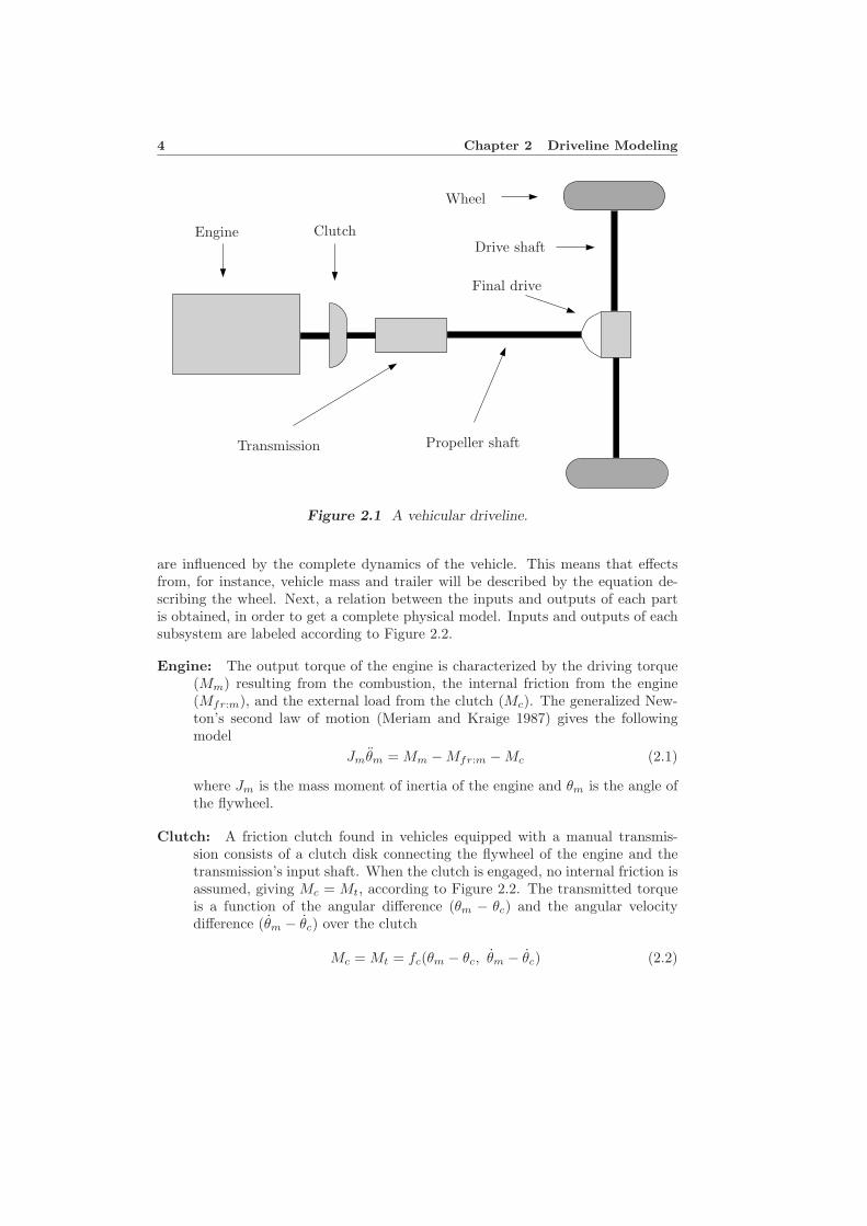
A vehicular driveline is depicted in Figure 2.1. It consists of an engine, clutch,transmission, propeller shaft, final drive, drive shafts, and wheels. In this sectionfundamental equations for the driveline will be derived. Furthermore, some basicequations regarding the forces acting on the wheel, are obtained. These equations
3
4 Chapter 2 Driveline Modeling
Engine Clutch
Transmission Propeller shaft
Final drive
Drive shaft
Wheel
Figure 2.1 A vehicular driveline.
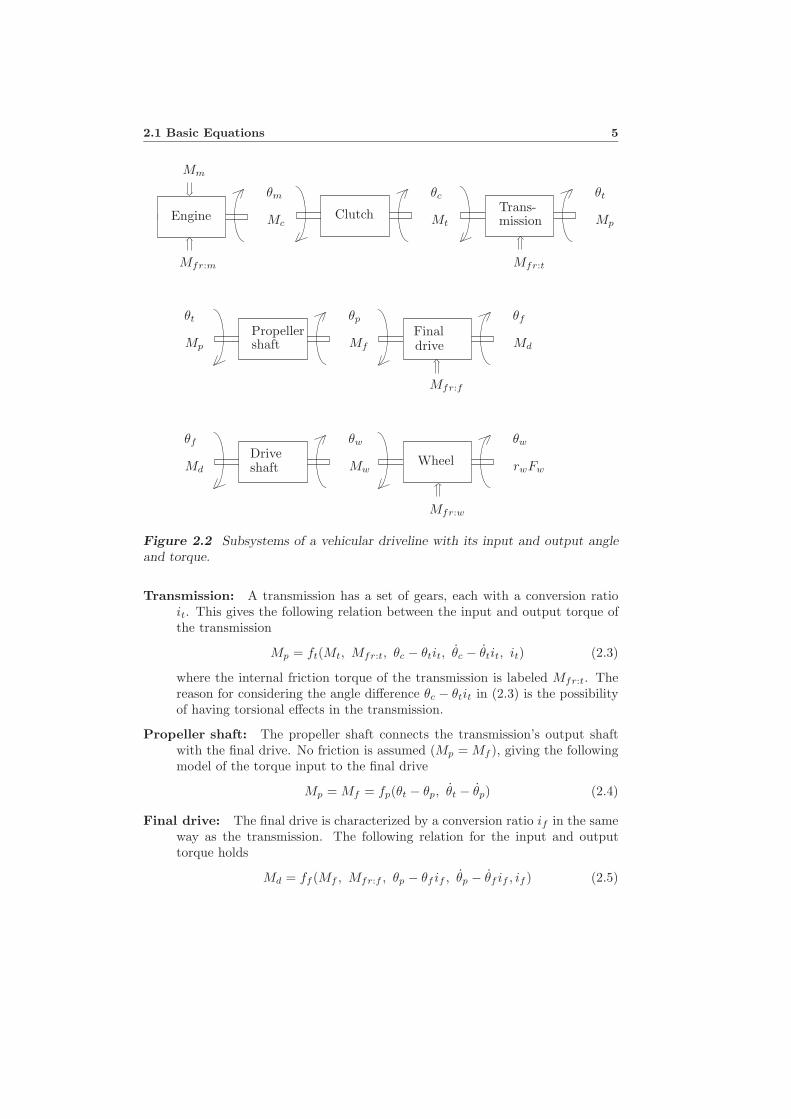
are influenced by the complete dynamics of the vehicle. This means that effectsfrom, for instance, vehicle mass and trailer will be described by the equation de-scribing the wheel. Next, a relation between the inputs and outputs of each partis obtained, in order to get a complete physical model. Inputs and outputs of eachsubsystem are labeled according to Figure 2.2.
Engine: The output torque of the engine is characterized by the driving torque(Mm) resulting from the combustion, the internal friction from the engine(Mfr:m), and the external load from the clutch (Mc). The generalized New-ton’s second law of motion (Meriam and Kraige 1987) gives the followingmodel
Jmθm = Mm − Mfr:m − Mc (2.1)
where Jm is the mass moment of inertia of the engine and θm is the angle ofthe flywheel.
Clutch: A friction clutch found in vehicles equipped with a manual transmis-sion consists of a clutch disk connecting the flywheel of the engine and thetransmission’s input shaft. When the clutch is engaged, no internal friction isassumed, giving Mc = Mt, according to Figure 2.2. The transmitted torqueis a function of the angular difference (θm − θc) and the angular velocitydifference (θm − θc) over the clutch
Mc = Mt = fc(θm − θc, θm − θc) (2.2)
2.1 Basic Equations 5
Md rwFw
θf θw
Wheel
Mm
Mfr:m
Mp
θt
Clutch Trans-
Mp Mf Md
θt θp θf
Engine
θm
Mt
θc
Mw
θw
Mfr:t
Mfr:f
Mfr:w
Mc mission
Propellershaft
Finaldrive
Driveshaft
Figure 2.2 Subsystems of a vehicular driveline with its input and output angleand torque.
Transmission: A transmission has a set of gears, each with a conversion ratioit. This gives the following relation between the input and output torque ofthe transmission
Mp = ft(Mt, Mfr:t, θc − θtit, θc − θtit, it) (2.3)
where the internal friction torque of the transmission is labeled Mfr:t. Thereason for considering the angle difference θc − θtit in (2.3) is the possibilityof having torsional effects in the transmission.
Propeller shaft: The propeller shaft connects the transmission’s output shaftwith the final drive. No friction is assumed (Mp = Mf ), giving the followingmodel of the torque input to the final drive
Mp = Mf = fp(θt − θp, θt − θp) (2.4)
Final drive: The final drive is characterized by a conversion ratio if in the sameway as the transmission. The following relation for the input and outputtorque holds
Md = ff (Mf , Mfr:f , θp − θf if , θp − θf if , if ) (2.5)
6 Chapter 2 Driveline Modeling
Fav
Fw Fr + mg sin(α)
Figure 2.3 Forces acting on a vehicle.
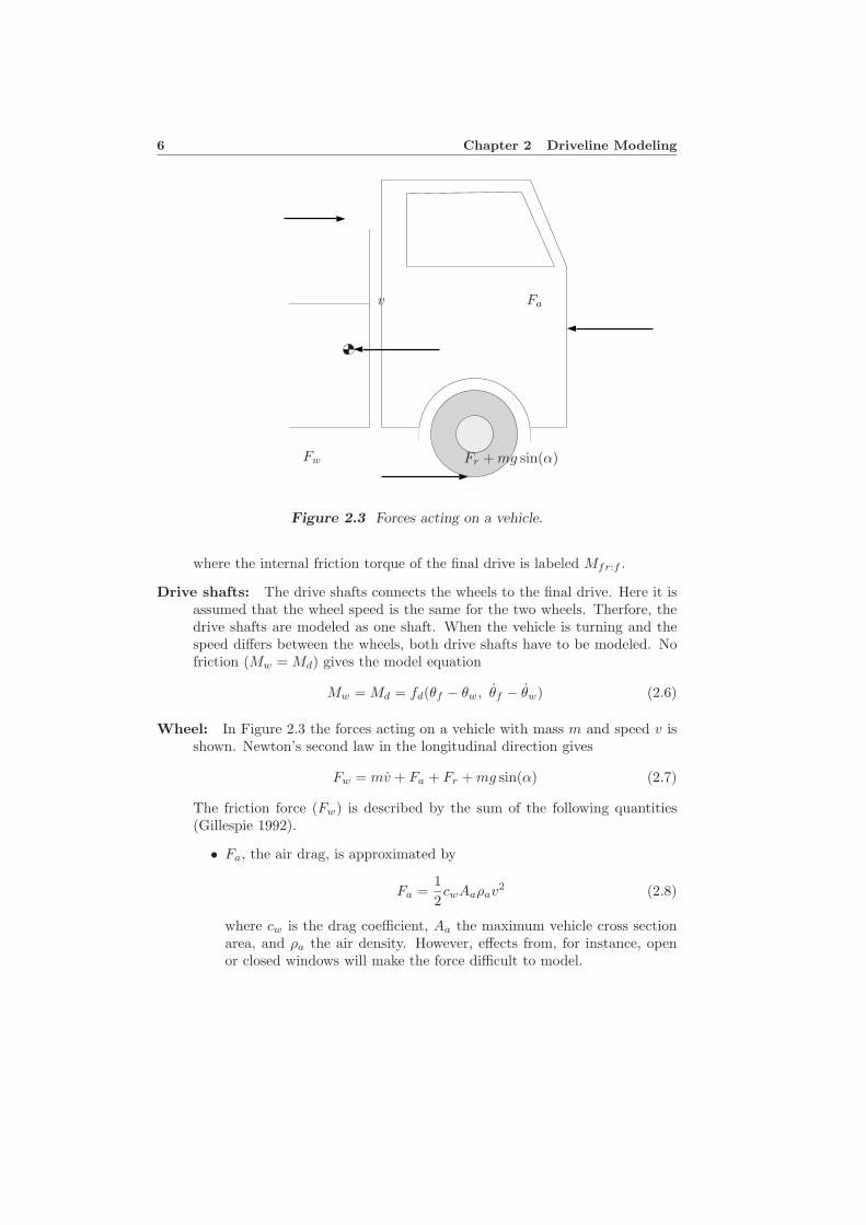
where the internal friction torque of the final drive is labeled Mfr:f .
Drive shafts: The drive shafts connects the wheels to the final drive. Here it isassumed that the wheel speed is the same for the two wheels. Therfore, thedrive shafts are modeled as one shaft. When the vehicle is turning and thespeed differs between the wheels, both drive shafts have to be modeled. Nofriction (Mw = Md) gives the model equation
Mw = Md = fd(θf − θw, θf − θw) (2.6)
Wheel: In Figure 2.3 the forces acting on a vehicle with mass m and speed v isshown. Newton’s second law in the longitudinal direction gives
Fw = mv + Fa + Fr + mg sin(α) (2.7)
The friction force (Fw) is described by the sum of the following quantities(Gillespie 1992).
• Fa, the air drag, is approximated by
Fa =12cwAaρav2 (2.8)
where cw is the drag coefficient, Aa the maximum vehicle cross sectionarea, and ρa the air density. However, effects from, for instance, openor closed windows will make the force difficult to model.
2.2 Shaft Flexibilities 7
• Fr, the rolling resistance, is approximated by
Fr = m(cr1 + cr2v) (2.9)
where cr1 and cr2 depends on, for instance, tires and tire pressure.
• mg sin(α), the gravitational force, where α is the slope of the road.
The coefficients of air drag and rolling resistance, (2.8) and (2.9), can be iden-tified e.g. by a identification scheme (Henriksson, Pettersson, and Gustafsson1993).
The resulting torque due to Fw is equal to Fwrw, where rw is the wheelradius. Newton’s second law gives
Jwθw = Mw − Fwrw − Mfr:w (2.10)
where Jw is the mass moment of inertia of the wheel, Mw is given by (2.6),and Mfr:w is the friction torque. Including (2.7) to (2.9) in (2.10) togetherwith v = rwθw gives
(Jw + mr2w)θw = Mw − Mfr:w − 1
2cwAaρar3
wθ2w (2.11)
−rwm(cr1 + cr2rwθw) − rwmgsin(α)
A complete model for the driveline with the clutch engaged is described byEquations (2.1) to (2.11). So far the functions fc, ft, fp, ff , fd, and the frictiontorques Mfr:t, Mfr:f , and Mfr:w are unknown. In the following section assumptionswill be made about the unknowns, resulting in a series of driveline models, withdifferent complexities.
2.2 Shaft Flexibilities
In the following two sections, assumptions will be made about the unknowns. First,a model with one torsional flexibility (the drive shaft) will be considered, and thena model with two torsional flexibilities (the drive shaft and propeller shaft) will beconsidered.
2.2.1 Model 1: Drive Shaft Flexibility
Assumptions about the fundamental equations in Section 2.1 are made in orderto obtain a model with drive shaft flexibility. Labels are according to Figure 2.2.The clutch and the propeller shafts are assumed to be stiff, and the drive shaft isdescribed as a damped torsional flexibility. The transmission and the final driveare assumed to multiply the torque with the conversion ratio, without losses.
8 Chapter 2 Driveline Modeling
Clutch: The clutch is assumed to be stiff, which gives the following equationsfor the torque and the angle
Mc = Mt, θm = θc (2.12)
Transmission: The transmission is described by one rotating inertia Jt. Thefriction torque is assumed to be described by a viscous damping coefficientbt. The model of the transmission, corresponding to (2.3), is
θc = θtit (2.13)Jtθt = Mtit − btθt − Mp (2.14)
By using (2.12) and (2.13), the model can be rewritten as
Jtθm = Mci2t − btθm − Mpit (2.15)
Propeller shaft: The propeller shaft is also assumed to be stiff, which gives thefollowing equations for the torque and the angle
Mp = Mf , θt = θp (2.16)
Final drive: In the same way as the transmission, the final drive is modeled byone rotating inertia Jf . The friction torque is assumed to be described by aviscous damping coefficient bf . The model of the final drive, correspondingto (2.5), is
θp = θf if (2.17)
Jf θf = Mf if − bf θf − Md (2.18)
Equation (2.18) can be rewritten with (2.16) and (2.17) which gives
Jf θt = Mpi2f − bf θt − Mdif (2.19)
Reducing (2.19) to engine speed is done by using (2.12) and (2.13) resultingin
Jf θm = Mpi2f it − bf θm − Mdif it (2.20)
By replacing Mp in (2.20) with Mp in (2.15), a model for the lumped trans-mission, propeller shaft, and final drive is obtained
(Jti2f + Jf )θm = Mci
2t i
2f − btθmi2f − bf θm − Mdif it (2.21)
Drive shaft: The drive shaft is modeled as a damped torsional flexibility, havingstiffness k, and internal damping c. Hence, (2.6) becomes
Mw = Md = k(θf − θw) + c(θf − θw) = k(θm/itif − θw) (2.22)
+ c(θm/itif − θw)
2.2 Shaft Flexibilities 9
θwθm
Jm + Jt/i2t + Jf/i2t i2f Jw + mr2
w
k
c
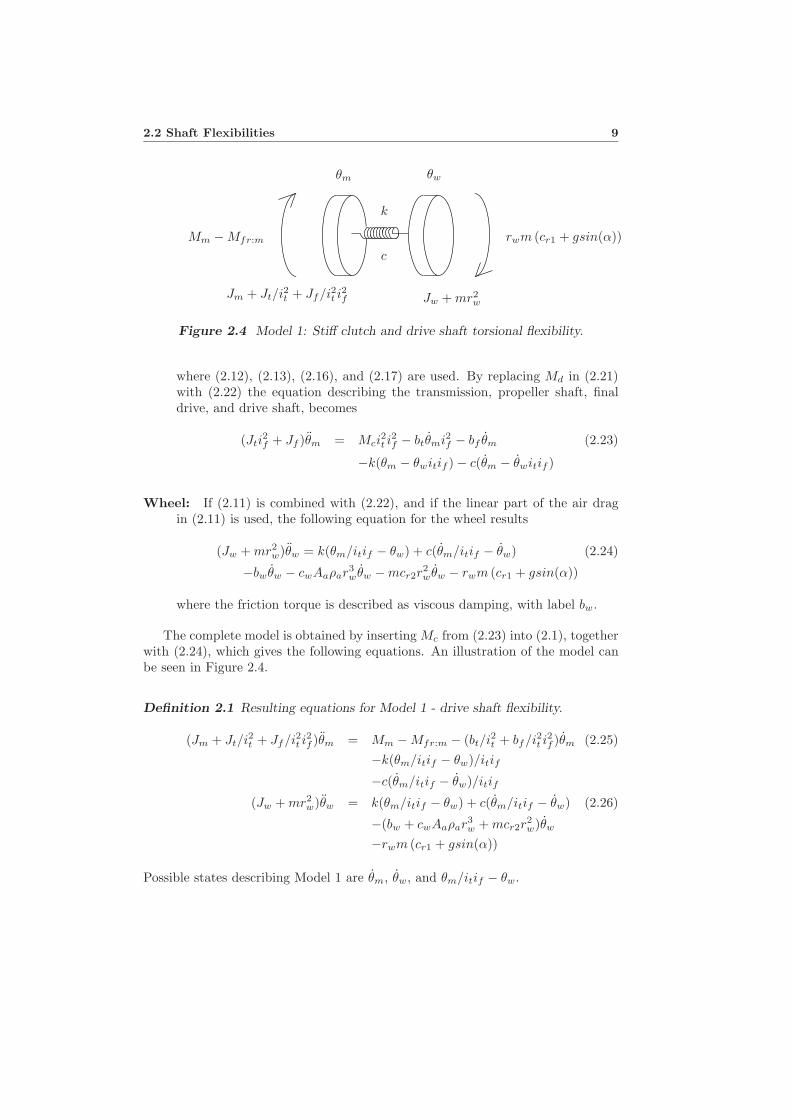
Mm − Mfr:m rwm (cr1 + gsin(α))
Figure 2.4 Model 1: Stiff clutch and drive shaft torsional flexibility.
where (2.12), (2.13), (2.16), and (2.17) are used. By replacing Md in (2.21)with (2.22) the equation describing the transmission, propeller shaft, finaldrive, and drive shaft, becomes
(Jti2f + Jf )θm = Mci
2t i
2f − btθmi2f − bf θm (2.23)
−k(θm − θwitif ) − c(θm − θwitif )
Wheel: If (2.11) is combined with (2.22), and if the linear part of the air dragin (2.11) is used, the following equation for the wheel results
(Jw + mr2w)θw = k(θm/itif − θw) + c(θm/itif − θw) (2.24)
−bwθw − cwAaρar3wθw − mcr2r
2wθw − rwm (cr1 + gsin(α))
where the friction torque is described as viscous damping, with label bw.
The complete model is obtained by inserting Mc from (2.23) into (2.1), togetherwith (2.24), which gives the following equations. An illustration of the model canbe seen in Figure 2.4.
Definition 2.1 Resulting equations for Model 1 - drive shaft flexibility.
(Jm + Jt/i2t + Jf/i2t i2f )θm = Mm − Mfr:m − (bt/i2t + bf/i2t i
2f )θm (2.25)
−k(θm/itif − θw)/itif
−c(θm/itif − θw)/itif
(Jw + mr2w)θw = k(θm/itif − θw) + c(θm/itif − θw) (2.26)
−(bw + cwAaρar3w + mcr2r
2w)θw
−rwm (cr1 + gsin(α))
Possible states describing Model 1 are θm, θw, and θm/itif − θw.
10 Chapter 2 Driveline Modeling
2.2.2 Model 1 Extended with a Flexible Propeller Shaft
It is also possible to consider two torsional flexibilities, the propeller shaft and thedrive shaft. In the derivation of the model, the clutch is assumed stiff, and thepropeller and drive shafts are modeled as damped torsional flexibilities. As in thederivation of Model 1, the transmission and final drive are assumed to multiply thetorque with the conversion ratio, without losses.
The derivation of Model 1 is repeated here with the difference that the modelfor the propeller shaft (2.16) is replaced by a model of a flexibility with stiffness kp
and internal damping cp
Mp = Mf = kp(θt − θp) + cp(θt − θp) = kp(θm/it − θp) + cp(θm/it − θp) (2.27)
where (2.12) and (2.13) are used in the last equality. This means that there aretwo torsional flexibilities, the propeller shaft and the drive shaft. Inserting (2.27)into (2.15) gives
Jtθm = Mci2t − btθm −
(kp(θm/it − θp) + cp(θm/it − θp)
)it (2.28)
By combining this with (2.1) the following differential equation describing thelumped engine and transmission results
(Jm + Jt/i2t )θm = Mm − Mfr:m − bt/i2t θm (2.29)
− 1it
(kp(θm/it − θp) + cp(θm/it − θp)
)
The final drive is described by inserting (2.27) in (2.18), and repeating (2.17)
θp = θf if (2.30)
Jf θf = if
(kp(θm/it − θp) + cp(θm/it − θp)
)− bf θf − Md (2.31)
Including (2.30) in (2.31) gives
Jf θp = i2f
(kp(θm/it − θp) + cp(θm/it − θp)
)− bf θp − ifMd (2.32)
The equation for the drive shaft (2.22) is repeated with new labels
Mw = Md = kd(θf − θw) + cd(θf − θw) = kd(θp/if − θw) + cd(θp/if − θw) (2.33)
where (2.30) is used in the last equality.The equation for the final drive (2.32) now becomes
Jf θp = i2f
(kp(θm/it − θp) + cp(θm/it − θp)
)− bf θp (2.34)
−if
(kd(θp/if − θw) + cd(θp/if − θw)
)
2.3 Models Including the Clutch 11
θwθm
Jm + Jt/i2t Jw + mr2w
kd
cd
Mm + Mfr:m rwm (cr1 + gsin(α))kp
cp
θp
Jf
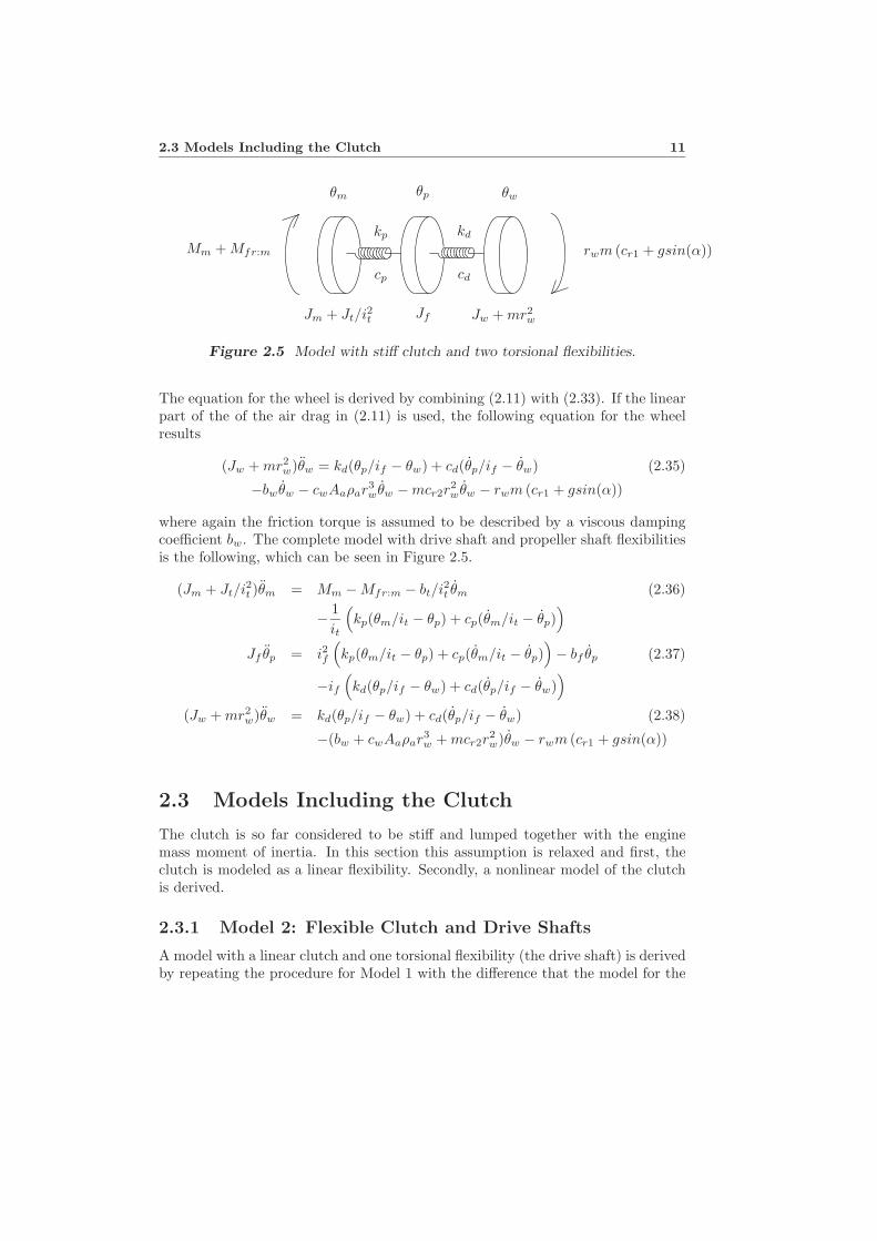
Figure 2.5 Model with stiff clutch and two torsional flexibilities.
The equation for the wheel is derived by combining (2.11) with (2.33). If the linearpart of the of the air drag in (2.11) is used, the following equation for the wheelresults
(Jw + mr2w)θw = kd(θp/if − θw) + cd(θp/if − θw) (2.35)
−bwθw − cwAaρar3wθw − mcr2r
2wθw − rwm (cr1 + gsin(α))
where again the friction torque is assumed to be described by a viscous dampingcoefficient bw. The complete model with drive shaft and propeller shaft flexibilitiesis the following, which can be seen in Figure 2.5.
(Jm + Jt/i2t )θm = Mm − Mfr:m − bt/i2t θm (2.36)
− 1it
(kp(θm/it − θp) + cp(θm/it − θp)
)
Jf θp = i2f
(kp(θm/it − θp) + cp(θm/it − θp)
)− bf θp (2.37)
−if
(kd(θp/if − θw) + cd(θp/if − θw)
)
(Jw + mr2w)θw = kd(θp/if − θw) + cd(θp/if − θw) (2.38)
−(bw + cwAaρar3w + mcr2r
2w)θw − rwm (cr1 + gsin(α))
2.3 Models Including the Clutch
The clutch is so far considered to be stiff and lumped together with the enginemass moment of inertia. In this section this assumption is relaxed and first, theclutch is modeled as a linear flexibility. Secondly, a nonlinear model of the clutchis derived.
2.3.1 Model 2: Flexible Clutch and Drive Shafts
A model with a linear clutch and one torsional flexibility (the drive shaft) is derivedby repeating the procedure for Model 1 with the difference that the model for the
12 Chapter 2 Driveline Modeling
clutch is a flexibility with stiffness kc and internal damping cc
Mc = Mt = kc(θm − θc) + cc(θm − θc) = kc(θm − θtit) + cc(θm − θtit) (2.39)
where (2.13) is used in the last equality. By inserting this into (2.1) the equationdescribing the engine inertia is given by
Jmθm = Mm − Mfr:m −(kc(θm − θtit) + cc(θm − θtit)
)(2.40)
Also by inserting (2.39) into (2.14), the equation describing the transmission is
Jtθt = it
(kc(θm − θtit) + cc(θm − θtit)
)− btθt − Mp (2.41)
Mp is derived from (2.19) giving
(Jt +Jf/i2f )θt = it
(kc(θm − θtit) + cc(θm − θtit)
)−(bt +bf/i2f )θt−Md/if (2.42)
which is the lumped transmission, propeller shaft, and final drive inertia.The drive shaft is modeled according to (2.22) as
Mw = Md = kd(θf − θw) + cd(θf − θw) = kd(θt/if − θw) + cd(θt/if − θw) (2.43)
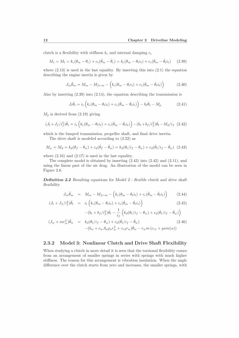
where (2.16) and (2.17) is used in the last equality.The complete model is obtained by inserting (2.43) into (2.42) and (2.11), and
using the linear part of the air drag. An illustration of the model can be seen inFigure 2.6.
Definition 2.2 Resulting equations for Model 2 - flexible clutch and drive shaftflexibility.
Jmθm = Mm − Mfr:m −(kc(θm − θtit) + cc(θm − θtit)
)(2.44)
(Jt + Jf/i2f )θt = it
(kc(θm − θtit) + cc(θm − θtit)
)(2.45)
−(bt + bf/i2f )θt − 1if
(kd(θt/if − θw) + cd(θt/if − θw)
)
(Jw + mr2w)θw = kd(θt/if − θw) + cd(θt/if − θw) (2.46)
−(bw + cwAaρar3w + cr2rw)θw − rwm (cr1 + gsin(α))
2.3.2 Model 3: Nonlinear Clutch and Drive Shaft Flexibility
When studying a clutch in more detail it is seen that the torsional flexibility comesfrom an arrangement of smaller springs in series with springs with much higherstiffness. The reason for this arrangement is vibration insulation. When the angledifference over the clutch starts from zero and increases, the smaller springs, with
2.3 Models Including the Clutch 13
θwθm
Jm Jw + mr2w
kd
cd
Mm + Mfr:m rwm (cr1 + gsin(α))kc
cc
θt
Jt + Jf/i2f
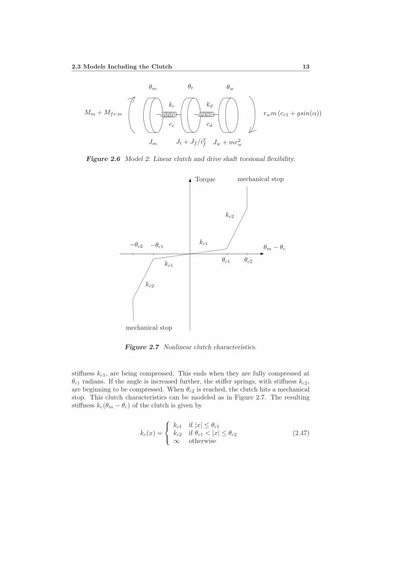
Figure 2.6 Model 2: Linear clutch and drive shaft torsional flexibility.
Torque
θm − θc
θc1 θc2
−θc1−θc2
mechanical stop
kc2
kc1
mechanical stop
kc2
kc1
Figure 2.7 Nonlinear clutch characteristics.
stiffness kc1, are being compressed. This ends when they are fully compressed atθc1 radians. If the angle is increased further, the stiffer springs, with stiffness kc2,are beginning to be compressed. When θc2 is reached, the clutch hits a mechanicalstop. This clutch characteristics can be modeled as in Figure 2.7. The resultingstiffness kc(θm − θc) of the clutch is given by
kc(x) =
kc1 if |x| ≤ θc1
kc2 if θc1 < |x| ≤ θc2
∞ otherwise(2.47)
14 Chapter 2 Driveline Modeling
2α
θ2θ1
k c
Figure 2.8 A shaft with stiffness k and internal damping c with a backlash of 2αrad.
The torque Mkc(θm − θc) from the clutch nonlinearity is
Mkc(x) =
kc1x if |x| ≤ θc1
kc1θc1 + kc2(x − θc1) if θc1 < x ≤ θc2
−kc1θc1 + kc2(x + θc1) if −θc2 < x ≤ −θc1
∞ otherwise
(2.48)
The nonlinear model is given by the following equations. The linear part of the airdrag is included, as in the previous models.
Definition 2.3 Resulting equations for Model 3 - nonlinear clutch and drive shaftflexibility.
Jmθm = Mm − Mfr:m − Mkc(θm − θtit) (2.49)
−cc(θm − θtit)
(Jt + Jf/i2f )θt = it
(Mkc(θm − θtit) + cc(θm − θtit)
)(2.50)
−(bt + bf/i2f )θt − 1if
(kd(θt/if − θw) + cd(θt/if − θw)
)
(Jw + mr2w)θw = kd(θt/if − θw) + cd(θt/if − θw) (2.51)
−(bw + mcr2rw + cwAaρar3w)θw − rwm (cr1 + gsin(α))
where Mkc(·) is given by (2.48) and cc denotes the damping coefficient of the clutch.
2.4 Additional Dynamics
For high speeds, the linear part of the air drag, is not sufficient. Then the differ-ential equation describing the wheel and the vehicle (2.26), (2.46), and (2.51) canbe changed to include the nonlinear model of the air drag, described in (2.8). The
2.4 Additional Dynamics 15
model describing the wheel is
(Jw + mr2w)θw = kd(θt/if − θw) + cd(θt/if − θw) (2.52)
−(bw + mcr2rw)θw − rwm (cr1 + gsin(α))
−12cwAaρar3
wθ2w
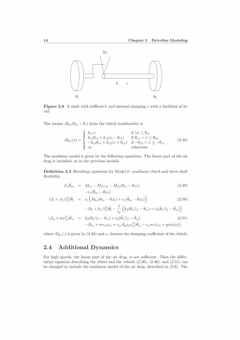
It is well known that elements like transmissions and drives introduce backlash.Throughout this thesis the dead zone model will be used (Liversidge 1952). Thetorque resulting from a shaft connected to a drive with backlash 2α is
M =
k(θ1 − θ2 − α) + c(θ1 − θ2) if θ1 − θ2 > α
k(θ1 − θ2 + α) + c(θ1 − θ2) if θ1 − θ2 < −α0 if |θ1 − θ2| < α
(2.53)
where k is the stiffness and c is the internal damping of the shaft, according toFigure 2.8.

16 Chapter 2 Driveline Modeling
3Field Trials and Modeling
Field trials are performed with a Scania truck. Different road slopes and gears aretested to study driveline resonances. The driving torque, engine speed, transmissionspeed, and wheel speed are measured. As mentioned already in Chapter 2, thesemeasurements are used to build models by extending an initial model structure byadding the effect that seems to be the major cause for the deviation still left. Therehas been some open questions regarding model structure in this study. One suchquestion is whether differences in engine speed and transmission speed is due toclutch dynamics or has other causes. The parameters of the models are estimated.The result is a series of models that describe the driveline in increasing detail.
3.1 The Truck
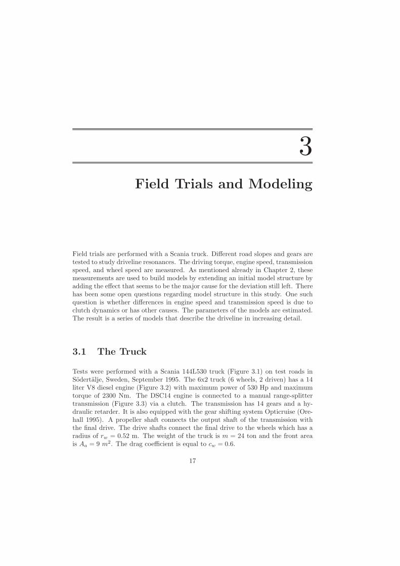
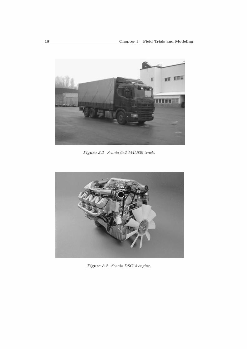
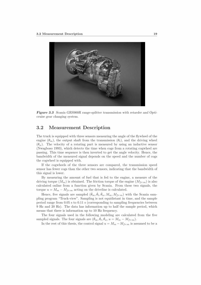
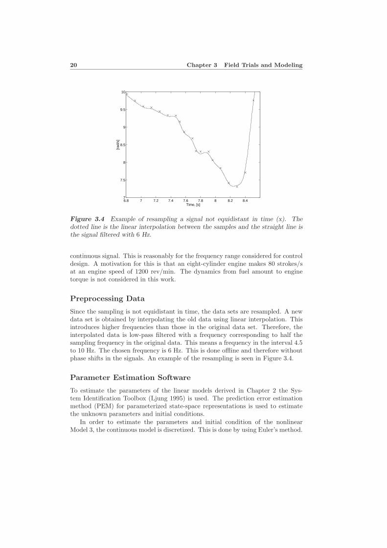
Tests were performed with a Scania 144L530 truck (Figure 3.1) on test roads inSodertalje, Sweden, September 1995. The 6x2 truck (6 wheels, 2 driven) has a 14liter V8 diesel engine (Figure 3.2) with maximum power of 530 Hp and maximumtorque of 2300 Nm. The DSC14 engine is connected to a manual range-splittertransmission (Figure 3.3) via a clutch. The transmission has 14 gears and a hy-draulic retarder. It is also equipped with the gear shifting system Opticruise (Ore-hall 1995). A propeller shaft connects the output shaft of the transmission withthe final drive. The drive shafts connect the final drive to the wheels which has aradius of rw = 0.52 m. The weight of the truck is m = 24 ton and the front areais Aa = 9 m2. The drag coefficient is equal to cw = 0.6.
17
18 Chapter 3 Field Trials and Modeling
Figure 3.1 Scania 6x2 144L530 truck.
Figure 3.2 Scania DSC14 engine.
3.2 Measurement Description 19
Figure 3.3 Scania GRS900R range-splitter transmission with retarder and Opti-cruise gear changing system.
3.2 Measurement Description
The truck is equipped with three sensors measuring the angle of the flywheel of theengine (θm), the output shaft from the transmission (θt), and the driving wheel(θw). The velocity of a rotating part is measured by using an inductive sensor(Nwagboso 1993), which detects the time when cogs from a rotating cogwheel arepassing. This time sequence is then inverted to get the angle velocity. Hence, thebandwidth of the measured signal depends on the speed and the number of cogsthe cogwheel is equipped with.
If the cogwheels of the three sensors are compared, the transmission speedsensor has fewer cogs than the other two sensors, indicating that the bandwidth ofthis signal is lower.
By measuring the amount of fuel that is fed to the engine, a measure of thedriving torque (Mm) is obtained. The friction torque of the engine (Mfr:m) is alsocalculated online from a function given by Scania. From these two signals, thetorque u = Mm − Mfr:m acting on the driveline is calculated.
Hence, five signals are sampled (θm, θt, θw,Mm,Mfr:m) with the Scania sam-pling program “Truck-view”. Sampling is not equidistant in time, and the sampleperiod range from 0.05 s to 0.11 s (corresponding to sampling frequencies between9 Hz and 20 Hz). The data has information up to half the sample period, whichmeans that there is information up to 10 Hz frequency.
The four signals used in the following modeling are calculated from the fivesampled signals. The four signals are (θm, θt, θw, u = Mm − Mfr:m).
In the rest of this thesis, the control signal u = Mm −Mfr:m is assumed to be a
20 Chapter 3 Field Trials and Modeling
6.8 7 7.2 7.4 7.6 7.8 8 8.2 8.47
7.5
8
8.5
9
9.5
10
Time, [s]
[rad
/s]
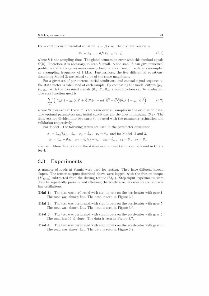
Figure 3.4 Example of resampling a signal not equidistant in time (x). Thedotted line is the linear interpolation between the samples and the straight line isthe signal filtered with 6 Hz.
continuous signal. This is reasonably for the frequency range considered for controldesign. A motivation for this is that an eight-cylinder engine makes 80 strokes/sat an engine speed of 1200 rev/min. The dynamics from fuel amount to enginetorque is not considered in this work.
Preprocessing Data
Since the sampling is not equidistant in time, the data sets are resampled. A newdata set is obtained by interpolating the old data using linear interpolation. Thisintroduces higher frequencies than those in the original data set. Therefore, theinterpolated data is low-pass filtered with a frequency corresponding to half thesampling frequency in the original data. This means a frequency in the interval 4.5to 10 Hz. The chosen frequency is 6 Hz. This is done offline and therefore withoutphase shifts in the signals. An example of the resampling is seen in Figure 3.4.
Parameter Estimation Software
To estimate the parameters of the linear models derived in Chapter 2 the Sys-tem Identification Toolbox (Ljung 1995) is used. The prediction error estimationmethod (PEM) for parameterized state-space representations is used to estimatethe unknown parameters and initial conditions.
In order to estimate the parameters and initial condition of the nonlinearModel 3, the continuous model is discretized. This is done by using Euler’s method.
3.3 Experiments 21
For a continuous differential equation, x = f(x, u), the discrete version is
xn = xn−1 + hf(xn−1, un−1) (3.1)
where h is the sampling time. The global truncation error with this method equalsO(h). Therefore it is necessary to keep h small. A too small h can give numericalproblems and it also gives unnecessarily long iteration time. The data is resampledat a sampling frequency of 1 kHz. Furthermore, the five differential equations,describing Model 3, are scaled to be of the same magnitude.
For a given set of parameters, initial conditions, and control signal sequence u,the state vector is calculated at each sample. By comparing the model output (ym,yt, yw) with the measured signals (θm, θt, θw) a cost function can be evaluated.The cost function used is∑
∀i
((θm(i) − ym(i))2 + i2t (θt(i) − yt(i))2 + i2t i
2f (θw(i) − yw(i))2
)(3.2)
where ∀i means that the sum is to taken over all samples in the estimation data.The optimal parameters and initial conditions are the ones minimizing (3.2). Thedata sets are divided into two parts to be used with the parameter estimation andvalidation respectively.
For Model 1 the following states are used in the parameter estimation
x1 = θm/itif − θw, x2 = θm, x3 = θw and for Models 2 and 3,
x1 = θm − θtit, x2 = θt/if − θw, x3 = θm, x4 = θt, x5 = θw
are used. More details about the state-space representation can be found in Chap-ter 4.
3.3 Experiments
A number of roads at Scania were used for testing. They have different knownslopes. The sensor outputs described above were logged, with the friction torque(Mfr:m) subtracted from the driving torque (Mm). Step input experiments weredone by repeatedly pressing and releasing the accelerator, in order to excite drive-line oscillations.
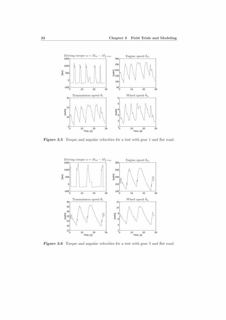
Trial 1: The test was performed with step inputs on the accelerator with gear 1.The road was almost flat. The data is seen in Figure 3.5.
Trial 2: The test was performed with step inputs on the accelerator with gear 5.The road was almost flat. The data is seen in Figure 3.6.
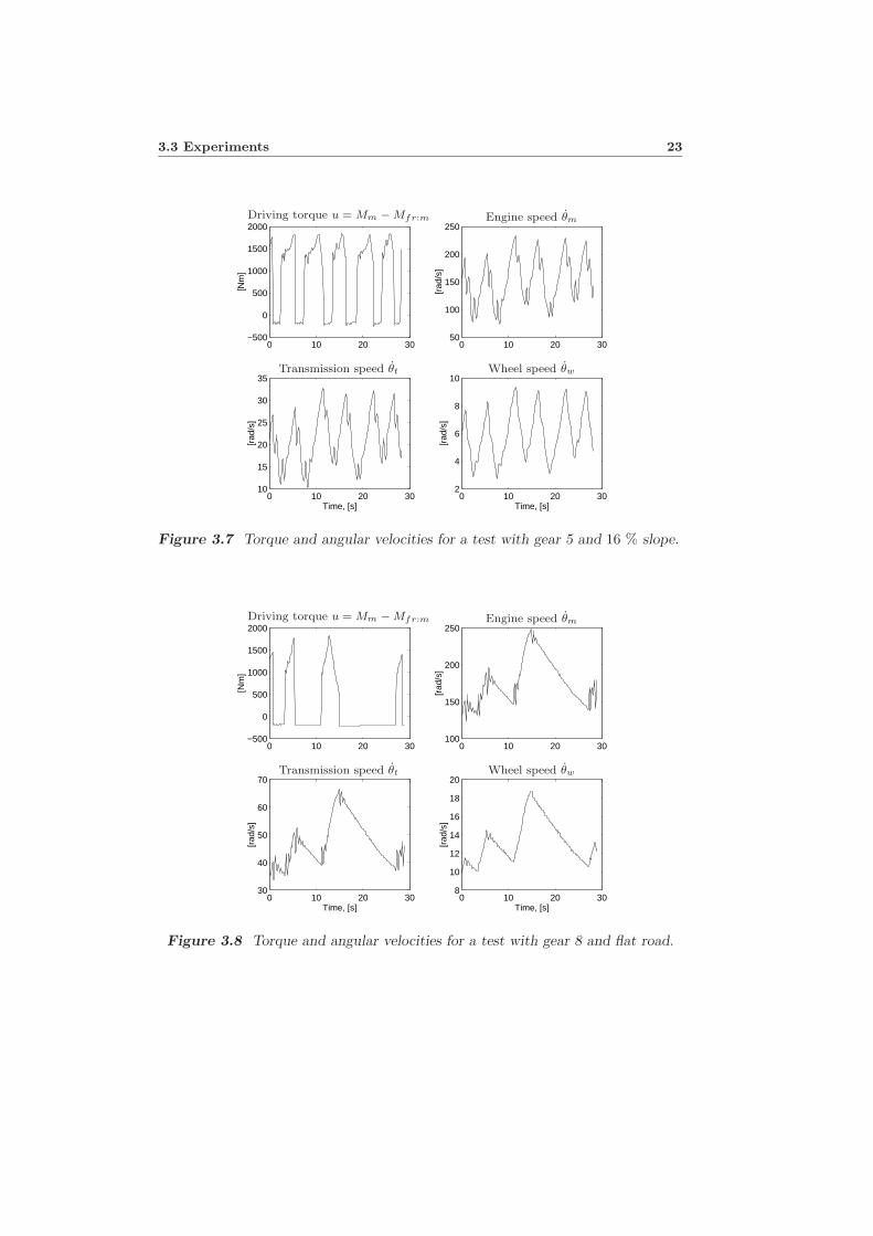
Trial 3: The test was performed with step inputs on the accelerator with gear 5.The road has 16 % slope. The data is seen in Figure 3.7.
Trial 4: The test was performed with step inputs on the accelerator with gear 8.The road was almost flat. The data is seen in Figure 3.8.
22 Chapter 3 Field Trials and Modeling
0 10 20 30−500
0
500
1000
1500
[Nm
]
0 10 20 3050
100
150
200
250
300
[rad
/s]
0 10 20 305
10
15
20
[rad
/s]
Time, [s]0 10 20 30
1
2
3
4
5
6
[rad
/s]
Time, [s]
Driving torque u = Mm − Mfr:m Engine speed θm
Transmission speed θt Wheel speed θw
Figure 3.5 Torque and angular velocities for a test with gear 1 and flat road.
0 10 20 30−500
0
500
1000
1500
[Nm
]
0 10 20 30100
150
200
250
300
[rad
/s]
0 10 20 3010
15
20
25
30
35
40
[rad
/s]
Time, [s]0 10 20 30
2
4
6
8
10
12
[rad
/s]
Time, [s]
Driving torque u = Mm − Mfr:m Engine speed θm
Transmission speed θt Wheel speed θw
Figure 3.6 Torque and angular velocities for a test with gear 5 and flat road.
3.3 Experiments 23
0 10 20 30−500
0
500
1000
1500
2000
[Nm
]
0 10 20 3050
100
150
200
250
[rad
/s]
0 10 20 3010
15
20
25
30
35
[rad
/s]
Time, [s]0 10 20 30
2
4
6
8
10
[rad
/s]
Time, [s]
Driving torque u = Mm − Mfr:m Engine speed θm
Transmission speed θt Wheel speed θw
Figure 3.7 Torque and angular velocities for a test with gear 5 and 16 % slope.
0 10 20 30−500
0
500
1000
1500
2000
[Nm
]
0 10 20 30100
150
200
250
[rad
/s]
0 10 20 3030
40
50
60
70
[rad
/s]
Time, [s]0 10 20 30
8
10
12
14
16
18
20
[rad
/s]
Time, [s]
Driving torque u = Mm − Mfr:m Engine speed θm
Transmission speed θt Wheel speed θw
Figure 3.8 Torque and angular velocities for a test with gear 8 and flat road.
24 Chapter 3 Field Trials and Modeling
3.4 Models
A number of driveline models were developed in Chapter 2. The choices made inthe modeling are now justified, by fitting the models to measured data. Besidesthe measured states (θm, θt, θw), the load and the states describing the torsion ofthe flexibilities are estimated by the models.
The data shown are from Trial 1, where the driveline oscillations are well ex-cited. Similar results are obtained from the other trials.
3.4.1 Influence from the Drive Shaft
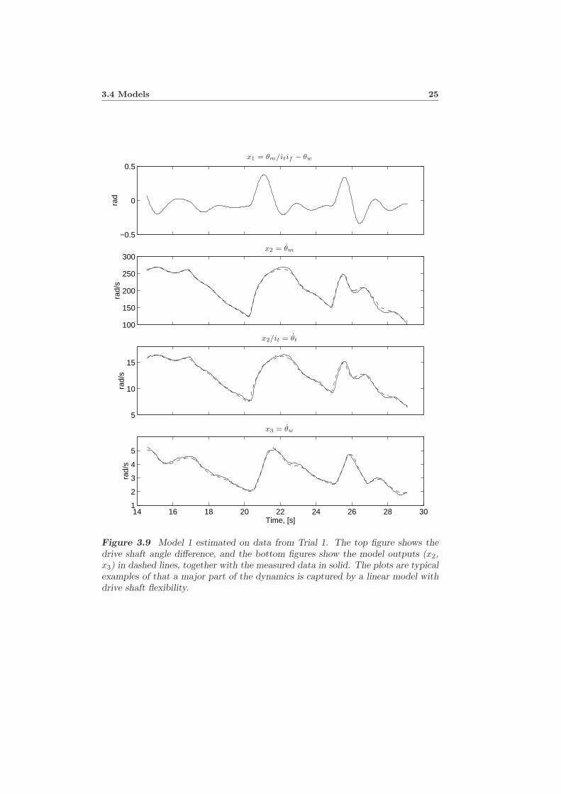
First, the influence from the drive shaft is investigated by estimating the parametersand initial conditions of Model 1. The engine speed and the wheel speed data isused to estimate the parameters. In Figure 3.9, the results from Trial 1 are shown.Here, also the transmission speed is plotted together with the model output enginespeed scaled with the conversion ratio in the transmission (it). The plots are typicalexamples that show that a major part of the driveline dynamics in the frequencyrange up to 6 Hz is captured with a linear mass-spring model with the drive shaftsas the main flexibility.
Result
• The main contribution to driveline dynamics from driving torque to enginespeed and wheel speed is the drive shaft.
• The true angle difference (x1 = θm/itif − θw) is unknown, but the valueestimated by the model has physically reasonable values.
• The model output transmission speed (x2/it) fits the measured transmissionspeed data well, but there are still deviations between model and measure-ment.
3.4.2 Influence from the Propeller Shaft
The model equations (2.36) to (2.38) describes Model 1 extended with the propellershaft with stiffness kp and damping cp. The three inertias in the model are
J1 = Jm + Jt/i2t
J2 = Jf (3.3)J3 = Jw + mr2
w
If the size of the three inertias are compared, the inertia of the final drive (Jf ) isconsiderably less than J1 and J2 in (3.3). Therefore, the model will act as if thereare two damped springs in series. The total stiffness of two undamped springs inseries is
k =kpi
2fkd
kpi2f + kd(3.4)
3.4 Models 25
−0.5
0
0.5
rad
100
150
200
250
300
rad/
s
5
10
15
rad/
s
14 16 18 20 22 24 26 28 301
2
3
4
5
rad/
s
Time, [s]
x1 = θm/itif − θw
x2 = θm
x2/it = θt
x3 = θw
Figure 3.9 Model 1 estimated on data from Trial 1. The top figure shows thedrive shaft angle difference, and the bottom figures show the model outputs (x2,x3) in dashed lines, together with the measured data in solid. The plots are typicalexamples of that a major part of the dynamics is captured by a linear model withdrive shaft flexibility.
26 Chapter 3 Field Trials and Modeling
whereas the total damping of two dampers in series is
c =cpi
2fcd
cpi2f + cd(3.5)
The damping and the stiffness of the drive shaft in the previous section will thustypically be underestimated due to the flexibility of the propeller shaft. This effectwill increase with lower conversion ratio in the final drive, if . The individualstiffness values obtained from parameter estimation are somewhat lower than thevalues obtained from material data.
3.4.3 Deviations between Engine Speed and TransmissionSpeed
As mentioned above, there is good agreement between model and experiments foru = Mm − Mfr:m, θm, and θw, but there is a slight deviation between measuredand estimated transmission speed. This deviation has a character of a phase shiftand some smoothing (signal levels and shapes agree). This indicates that thereis some additional dynamics between engine speed, θm, and transmission speed,θt. Two natural candidates are additional mass-spring dynamics in the driveline,or sensor dynamics. The explanation is that there is a combined effect, with themajor difference explained by the sensor dynamics. The motivation for this is thatthe high stiffness of the clutch flexibility (given from material data) can not resultin a difference of a phase shift form. Neither can backlash in the transmissionexplain the difference, because then the engine and transmission speeds would beequal when the backlash is at its endpoint.
As mentioned before, the bandwidth of the measured transmission speed is lowerthan the measured engine and wheel speeds, due to fewer cogs in the sensor. It isassumed that the engine speed and wheel speed sensor dynamics are not influencingthe data for frequencies up to 6 Hz. The speed dependence of the transmissionsensor dynamics is neglected. The following sensor dynamics are assumed, aftersome comparison between sensor filters of different order,
fm = 1
ft =1
1 + αs(3.6)
fw = 1
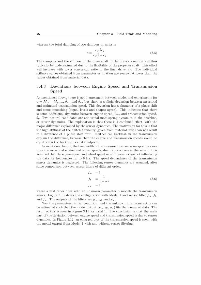
where a first order filter with an unknown parameter α models the transmissionsensor. Figure 3.10 shows the configuration with Model 1 and sensor filter fm, ft,and fw. The outputs of the filters are ym, yt, and yw.
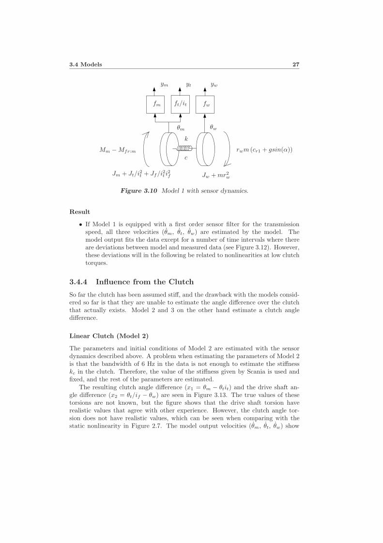
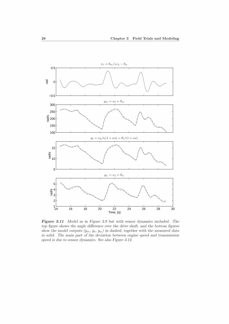
Now the parameters, initial condition, and the unknown filter constant α canbe estimated such that the model output (ym, yt, yw) fits the measured data. Theresult of this is seen in Figure 3.11 for Trial 1. The conclusion is that the mainpart of the deviation between engine speed and transmission speed is due to sensordynamics. In Figure 3.12, an enlarged plot of the transmission speed is seen, withthe model output from Model 1 with and without sensor filtering.
3.4 Models 27
θwθm
Jm + Jt/i2t + Jf/i2t i2f Jw + mr2
w
k
cMm − Mfr:m rwm (cr1 + gsin(α))
fw
yw
fm
ym
ft/it
yt
Figure 3.10 Model 1 with sensor dynamics.
Result
• If Model 1 is equipped with a first order sensor filter for the transmissionspeed, all three velocities (θm, θt, θw) are estimated by the model. Themodel output fits the data except for a number of time intervals where thereare deviations between model and measured data (see Figure 3.12). However,these deviations will in the following be related to nonlinearities at low clutchtorques.
3.4.4 Influence from the Clutch
So far the clutch has been assumed stiff, and the drawback with the models consid-ered so far is that they are unable to estimate the angle difference over the clutchthat actually exists. Model 2 and 3 on the other hand estimate a clutch angledifference.
Linear Clutch (Model 2)
The parameters and initial conditions of Model 2 are estimated with the sensordynamics described above. A problem when estimating the parameters of Model 2is that the bandwidth of 6 Hz in the data is not enough to estimate the stiffnesskc in the clutch. Therefore, the value of the stiffness given by Scania is used andfixed, and the rest of the parameters are estimated.
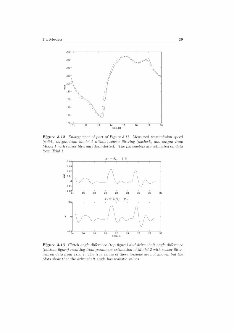
The resulting clutch angle difference (x1 = θm − θtit) and the drive shaft an-gle difference (x2 = θt/if − θw) are seen in Figure 3.13. The true values of thesetorsions are not known, but the figure shows that the drive shaft torsion haverealistic values that agree with other experience. However, the clutch angle tor-sion does not have realistic values, which can be seen when comparing with thestatic nonlinearity in Figure 2.7. The model output velocities (θm, θt, θw) show
28 Chapter 3 Field Trials and Modeling
−0.5
0
0.5
rad
100
150
200
250
300
rad/
s
5
10
15
rad/
s
14 16 18 20 22 24 26 28 301
2
3
4
5
rad/
s
Time, [s]
x1 = θm/itif − θw
ym = x2 = θm
yt = x2/it(1 + αs) = θt/(1 + αs)
yw = x3 = θw
Figure 3.11 Model as in Figure 3.9 but with sensor dynamics included. Thetop figure shows the angle difference over the drive shaft, and the bottom figuresshow the model outputs (ym, yt, yw) in dashed, together with the measured datain solid. The main part of the deviation between engine speed and transmissionspeed is due to sensor dynamics. See also Figure 3.12.
3.4 Models 29
11 12 13 14 15 16 17 18100
120
140
160
180
200
220
240
260
280
Time, [s]
rad/
s
Figure 3.12 Enlargement of part of Figure 3.11. Measured transmission speed(solid), output from Model 1 without sensor filtering (dashed), and output fromModel 1 with sensor filtering (dash-dotted). The parameters are estimated on datafrom Trial 1.
14 16 18 20 22 24 26 28 30−0.02
−0.01
0
0.01
0.02
0.03
0.04
rad
14 16 18 20 22 24 26 28 30−0.5
0
0.5
rad
Time, [s]
x1 = θm − θtit
x2 = θt/if − θw
Figure 3.13 Clutch angle difference (top figure) and drive shaft angle difference(bottom figure) resulting from parameter estimation of Model 2 with sensor filter-ing, on data from Trial 1. The true values of these torsions are not known, but theplots show that the drive shaft angle has realistic values.
30 Chapter 3 Field Trials and Modeling
14 16 18 20 22 24 26 28 30
0rad
14 16 18 20 22 24 26 28 30−0.5
0
0.5
rad
Time, [s]
−θc1
θc1
x1 = θm/it − θt
x2 = θt/if − θw
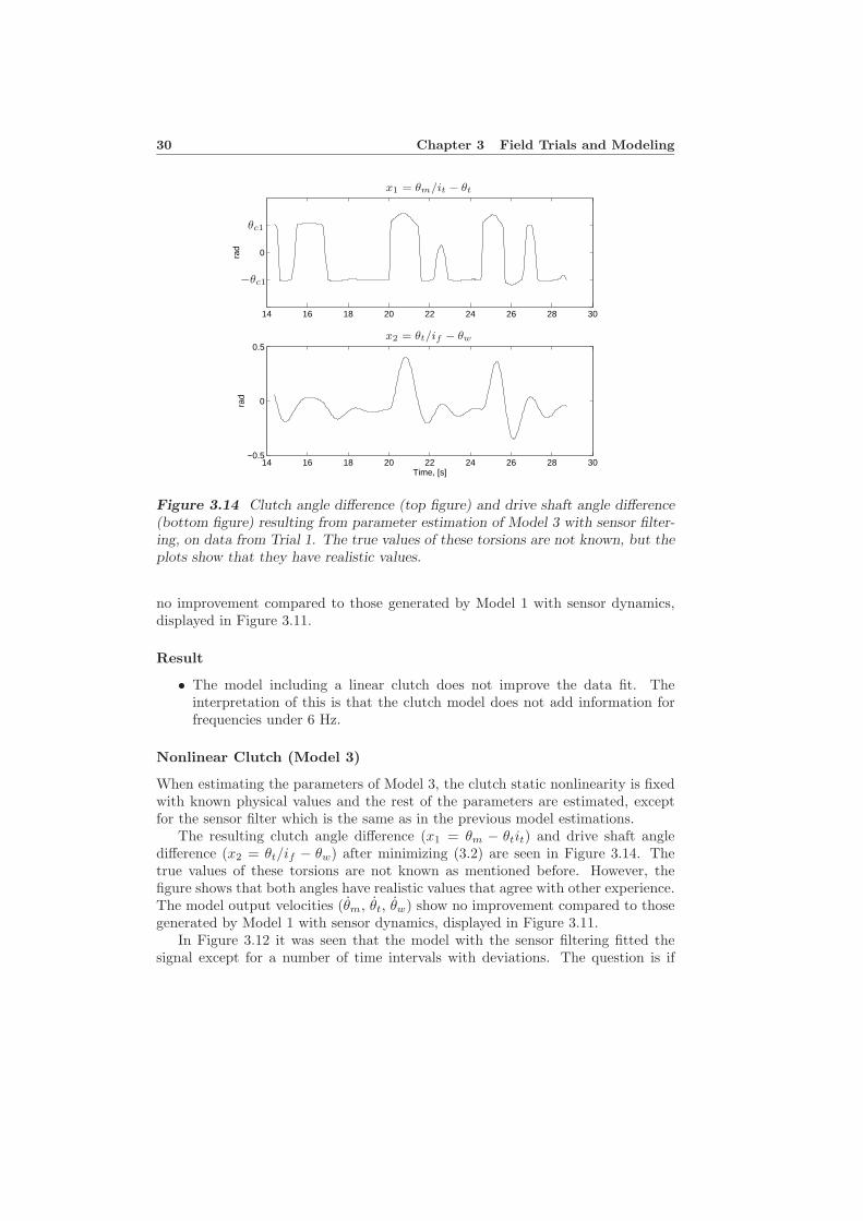
Figure 3.14 Clutch angle difference (top figure) and drive shaft angle difference(bottom figure) resulting from parameter estimation of Model 3 with sensor filter-ing, on data from Trial 1. The true values of these torsions are not known, but theplots show that they have realistic values.
no improvement compared to those generated by Model 1 with sensor dynamics,displayed in Figure 3.11.
Result
• The model including a linear clutch does not improve the data fit. Theinterpretation of this is that the clutch model does not add information forfrequencies under 6 Hz.
Nonlinear Clutch (Model 3)
When estimating the parameters of Model 3, the clutch static nonlinearity is fixedwith known physical values and the rest of the parameters are estimated, exceptfor the sensor filter which is the same as in the previous model estimations.
The resulting clutch angle difference (x1 = θm − θtit) and drive shaft angledifference (x2 = θt/if − θw) after minimizing (3.2) are seen in Figure 3.14. Thetrue values of these torsions are not known as mentioned before. However, thefigure shows that both angles have realistic values that agree with other experience.The model output velocities (θm, θt, θw) show no improvement compared to thosegenerated by Model 1 with sensor dynamics, displayed in Figure 3.11.
In Figure 3.12 it was seen that the model with the sensor filtering fitted thesignal except for a number of time intervals with deviations. The question is if
3.4 Models 31
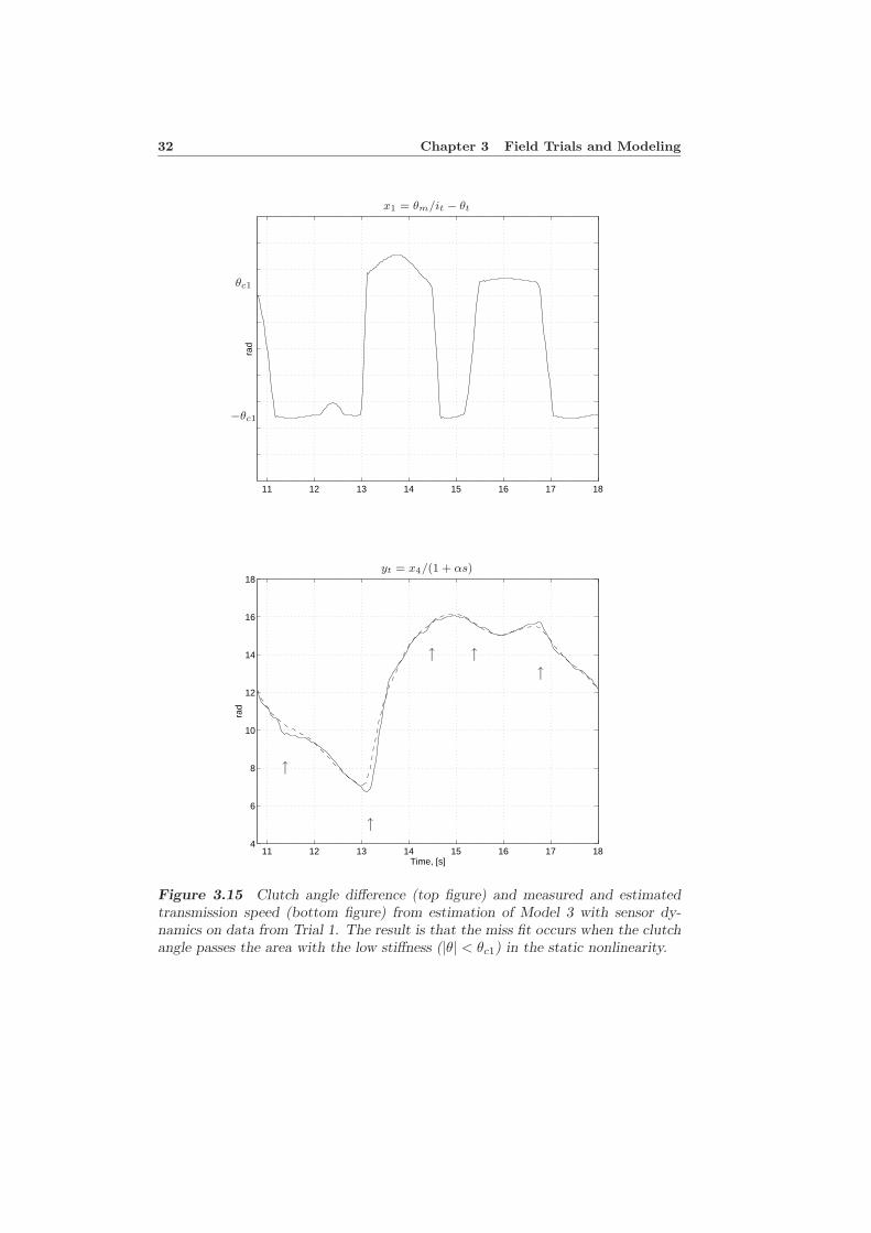
this is a result of some nonlinearity. Figure 3.15 shows the transmission speedplotted together with the model output and the clutch angle torsion. It is clearfrom Figure 3.15 that the deviation between model and experiments occurs whenthe clutch angle passes the area with the low stiffness in the static nonlinearity (seeFigure 2.7).
Result
• The model including the nonlinear clutch does not improve the data fit forfrequencies up to 6 Hz.
• The model is able to estimate a clutch angle with realistic values.
• The estimated clutch angle shows that when the clutch passes the area withlow stiffness in the nonlinearity, the model deviates from the data. Thereason is unmodeled dynamics at low clutch torques (Bjornberg, Pettersson,and Nielsen 1996).
3.4.5 Model Validity
As mentioned before, the data sets are divided into two parts. The parameters areestimated on the estimation data. The results are then evaluated on the validationdata, and these are the results shown in this chapter.
In the parameter estimation, the unknown load l, which vary between the tri-als, is estimated. The load can be recalculated to estimate road slope, and thecalculated values agree well with the known values of the road slopes at Scania.Furthermore, the estimation of the states describing the torsion of the clutch andthe drive shaft shows realistic values. This gives further support to model structureand parameters.
The assumption about sensor dynamics in the transmission speed influencingthe experiments, agrees well with the fact that the engine speed sensor and thewheel speed sensor have considerably higher bandwidth (more cogs) than the trans-mission speed sensor.
When estimating the parameters of the models investigated, there is a problemwith identifying the viscous friction components b. The sensitivity in the model tovariations in the friction parameters is low, and the same model fit can be obtainedfor a range of frictions parameters.
32 Chapter 3 Field Trials and Modeling
11 12 13 14 15 16 17 18
rad
11 12 13 14 15 16 17 184
6
8
10
12
14
16
18
rad
Time, [s]
θc1
−θc1
x1 = θm/it − θt
↑
↑
↑ ↑↑
yt = x4/(1 + αs)
Figure 3.15 Clutch angle difference (top figure) and measured and estimatedtransmission speed (bottom figure) from estimation of Model 3 with sensor dy-namics on data from Trial 1. The result is that the miss fit occurs when the clutchangle passes the area with the low stiffness (|θ| < θc1) in the static nonlinearity.
3.5 Summary 33
3.5 Summary
Parameter estimation of the models derived in Chapter 2 shows that a model withone torsional flexibility and two inertias is able to fit the measured engine speedand wheel speed. By considering the difference between the measured transmissionspeed and wheel speed it is reasonably to deduce that the main flexibility is thedrive shafts.
In order for the model to fit the data from all three measured velocities, afirst order sensor filter is added to the model, in accordance with properties ofthe sensory system. It is shown that all three velocities are fitted. Parameterestimation of a model with a nonlinear clutch explains that the difference betweenthe measured data and the model occurs when the clutch transfers zero torque.
Further supporting facts of the models are that they give values to the non-measured variables, drive shaft and clutch torsion, that agree with experience fromother sources. Furthermore, the known road slopes are well estimated.
The result is a series of models that describe the driveline in increasing detailby, in each extension, adding the effect that seems to be the major cause for thedeviation still left.
The result, from a user perspective, is that, within the frequency regime in-teresting for control design, the mass-spring models with some sensor dynamics(Model 1 and Model 2) give good agreement with experiments. They are thus suit-able for control design. The major deviations left are captured by the nonlineareffects in Model 3 which makes this model suitable for verifying simulation studiesin control design.

34 Chapter 3 Field Trials and Modeling
4Architectural Issues for Driveline
Control
As seen in the previous chapters, there are significant torsional resonances in adriveline. Active control of these resonances is the topic of the rest of this thesis.Chapters 5 and 6 treats two different problems. Besides formulating the controlproblem in this chapter, there is one architectural issue that will be given specialattention. There are different possible choices in driveline control between usingdifferent sensor locations, e.g. engine speed sensor, transmission speed sensor,or wheel speed sensor. If the driveline were rigid, the choice would not matter,since the sensor outputs would differ only by a scaling factor. However, it will bedemonstrated that the presence of torsional flexibilities implies that sensor choicegives different control problems. The difference can be formulated in control the-oretic terms e.g. by saying that the poles are the same, but the zeros differ bothin number and values. The issue of sensor location seems to be a little studiedtopic (Kubrusly and Malebranche 1985; Ljung 1988), even though its relevance forcontrol characteristics.
The driveline model equations in Chapter 2 are written in state-space form inSection 4.1. The formulation of performance output and controller structures usedin the rest of the thesis are given in Section 4.2. Control of resonant systems withsimple controllers is known to have structural properties e.g. with respect to sensorlocation (Spong and Vidyasagar 1989), as mentioned before. In Section 4.3, thesedifferences are illustrated for driveline models. In Section 4.4, forming the maincontribution of this chapter, an investigation about how these properties transferswhen using more complicated controller structures like LQG/LTR is made. Thispart is based on the material in Pettersson and Nielsen (1995).
35
36 Chapter 4 Architectural Issues for Driveline Control
4.1 State-Space Formulation
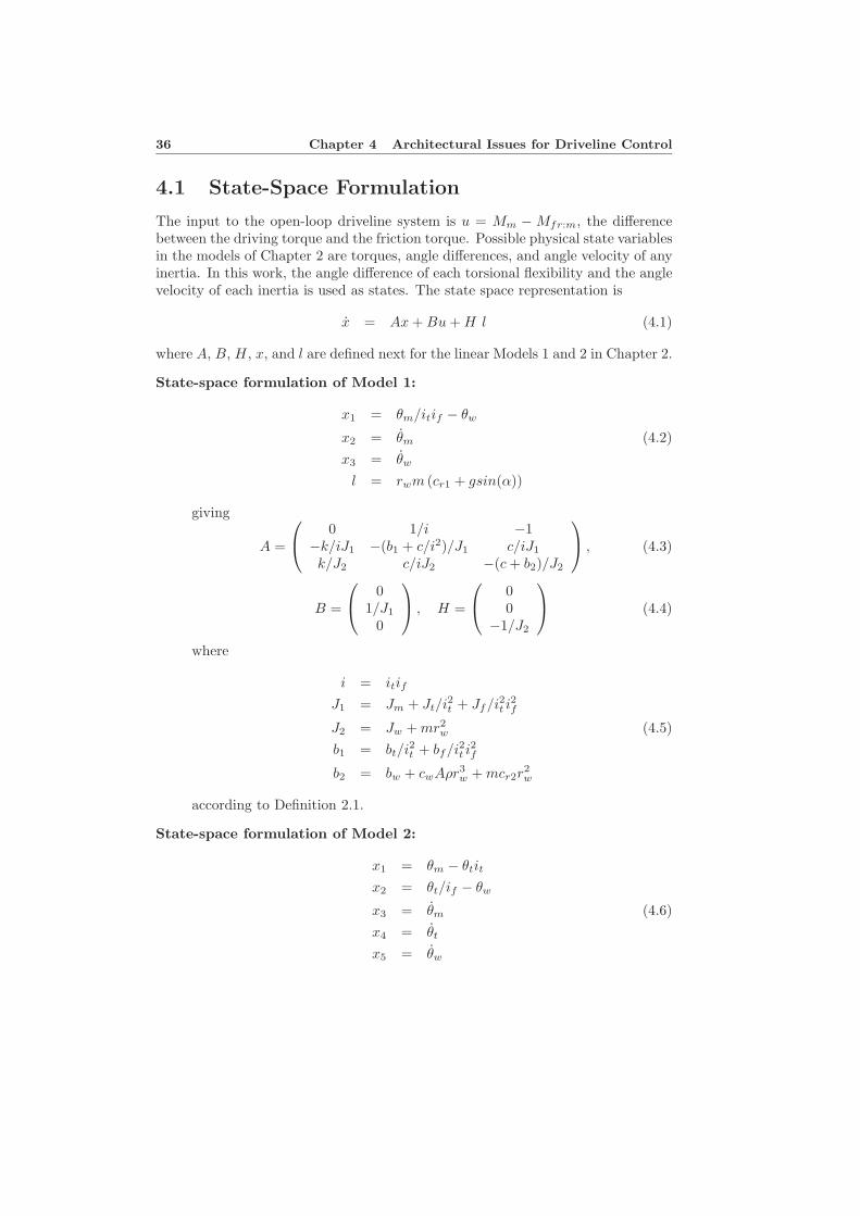
The input to the open-loop driveline system is u = Mm − Mfr:m, the differencebetween the driving torque and the friction torque. Possible physical state variablesin the models of Chapter 2 are torques, angle differences, and angle velocity of anyinertia. In this work, the angle difference of each torsional flexibility and the anglevelocity of each inertia is used as states. The state space representation is
x = Ax + Bu + H l (4.1)
where A, B, H, x, and l are defined next for the linear Models 1 and 2 in Chapter 2.
State-space formulation of Model 1:
x1 = θm/itif − θw
x2 = θm (4.2)x3 = θw
l = rwm (cr1 + gsin(α))
giving
A =
0 1/i −1
−k/iJ1 −(b1 + c/i2)/J1 c/iJ1
k/J2 c/iJ2 −(c + b2)/J2
, (4.3)
B =
0
1/J1
0
, H =
0
0−1/J2
(4.4)
where
i = itif
J1 = Jm + Jt/i2t + Jf/i2t i2f
J2 = Jw + mr2w (4.5)
b1 = bt/i2t + bf/i2t i2f
b2 = bw + cwAρr3w + mcr2r
2w
according to Definition 2.1.
State-space formulation of Model 2:
x1 = θm − θtit
x2 = θt/if − θw
x3 = θm (4.6)x4 = θt
x5 = θw
4.1 State-Space Formulation 37
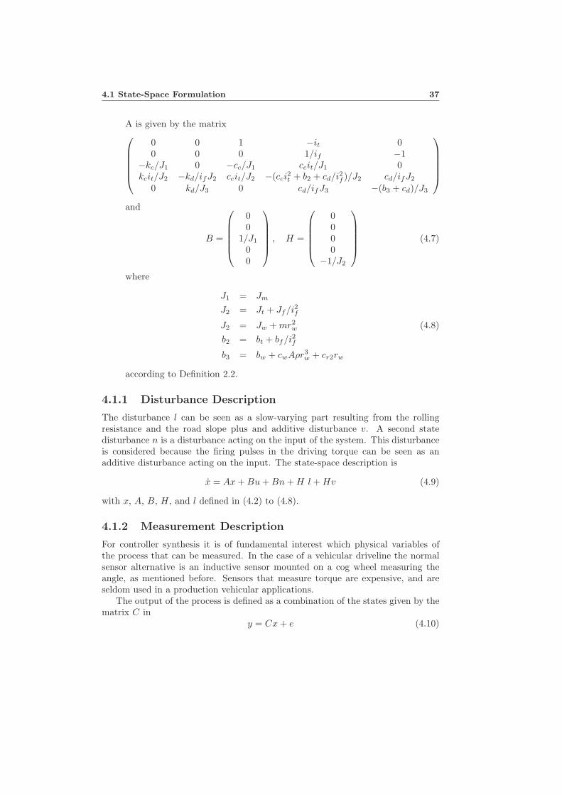
A is given by the matrix
0 0 1 −it 00 0 0 1/if −1
−kc/J1 0 −cc/J1 ccit/J1 0kcit/J2 −kd/ifJ2 ccit/J2 −(cci
2t + b2 + cd/i2f )/J2 cd/ifJ2
0 kd/J3 0 cd/ifJ3 −(b3 + cd)/J3
and
B =
00
1/J1
00
, H =
0000
−1/J2
(4.7)
where
J1 = Jm
J2 = Jt + Jf/i2f
J2 = Jw + mr2w (4.8)
b2 = bt + bf/i2f
b3 = bw + cwAρr3w + cr2rw
according to Definition 2.2.
4.1.1 Disturbance Description
The disturbance l can be seen as a slow-varying part resulting from the rollingresistance and the road slope plus and additive disturbance v. A second statedisturbance n is a disturbance acting on the input of the system. This disturbanceis considered because the firing pulses in the driving torque can be seen as anadditive disturbance acting on the input. The state-space description is
x = Ax + Bu + Bn + H l + Hv (4.9)
with x, A, B, H, and l defined in (4.2) to (4.8).
4.1.2 Measurement Description
For controller synthesis it is of fundamental interest which physical variables ofthe process that can be measured. In the case of a vehicular driveline the normalsensor alternative is an inductive sensor mounted on a cog wheel measuring theangle, as mentioned before. Sensors that measure torque are expensive, and areseldom used in a production vehicular applications.
The output of the process is defined as a combination of the states given by thematrix C in
y = Cx + e (4.10)
38 Chapter 4 Architectural Issues for Driveline Control
Fy(s)
M
C
e
zxu
y
1/s
A
Bx
Fr(s)r
D
Hl + v
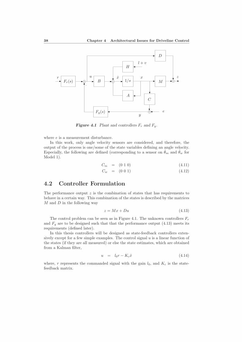
Figure 4.1 Plant and controllers Fr and Fy.
where e is a measurement disturbance.In this work, only angle velocity sensors are considered, and therefore, the
output of the process is one/some of the state variables defining an angle velocity.Especially, the following are defined (corresponding to a sensor on θm and θw forModel 1).
Cm = (0 1 0) (4.11)Cw = (0 0 1) (4.12)
4.2 Controller Formulation
The performance output z is the combination of states that has requirements tobehave in a certain way. This combination of the states is described by the matricesM and D in the following way
z = Mx + Du (4.13)
The control problem can be seen as in Figure 4.1. The unknown controllers Fr
and Fy are to be designed such that that the performance output (4.13) meets itsrequirements (defined later).
In this thesis controllers will be designed as state-feedback controllers exten-sively except for a few simple examples. The control signal u is a linear function ofthe states (if they are all measured) or else the state estimates, which are obtainedfrom a Kalman filter,
u = l0r − Kcx (4.14)
where, r represents the commanded signal with the gain l0, and Kc is the state-feedback matrix.
4.3 Some Feedback Properties 39
Identifying the matrices Fr(s) and Fy(s) in Figure 4.1 gives
Fy(s) = Kc(sI − A + BKc + KfC)−1Kf (4.15)Fr(s) = l0
(1 − Kc(sI − A + BKc + KfC)−1B
)
The closed-loop transfer functions from r, v, and e to the control signal u aregiven by
Gru =(I − Kc(sI − A + BKc)−1B
)l0r (4.16)
Gvu = Kc(sI − A + KfC)−1N − Kc(sI − A + BKc)−1N (4.17)−Kc(sI − A + BKc)−1BKc(sI − A + KfC)−1N
Geu = Kc
((sI − A + BKc)−1BKc − I
)(sI − A + KfC)−1Kf (4.18)
The transfer functions to the performance output z are given by
Grz = (M(sI − A)−1B + D)Gru (4.19)Gvz = M(sI − A + BKc)−1BKc(sI − A + KfC)−1N (4.20)
+M(sI − A + BKc)−1N + DGwu
Gez = (M(sI − A)−1B + D)Gvu (4.21)
Two return ratios results, which characterizes the closed-loop behavior at theplant output and input respectively
GFy = C(sI − A)−1BFy (4.22)FyG = FyC(sI − A)−1B (4.23)
When only one sensor is used, these return ratios are scalar and thus equal.LQG/LTR is not directly applicable to driveline control with more than one
sensor as input to the observer. This is because there are unequal number of sensorsand control signals. Therefore, it is important with the type of investigation aboutthe structural properties made in this chapter, when extending to more sensors.This is however not considered in this work.
4.3 Some Feedback Properties
The performance output when controlling the driveline to a certain speed is thevelocity of the wheel, defined as
z = θw = Cwx (4.24)
When studying the closed-loop control problem with a sensor on θm or θw, twodifferent control problems results. In Figure 4.2 a root locus with respect to aP-controller gain is seen for two gears using velocity sensor θm and θw respectively.The open-loop transfer functions from u to engine speed Gum has three poles and
40 Chapter 4 Architectural Issues for Driveline Control
−10 −5 0−6
−4
−2
0
2
4
6
Imag
−10 −5 0−6
−4
−2
0
2
4
6
Imag
−20 −10 0−15
−10
−5
0
5
10
15
Imag
Real−20 −10 0
−15
−10
−5
0
5
10
15Im
ag
Real
Gear 1 and θm feedback Gear 1 and θw feedback
Gear 8 and θm feedback Gear 8 and θw feedback
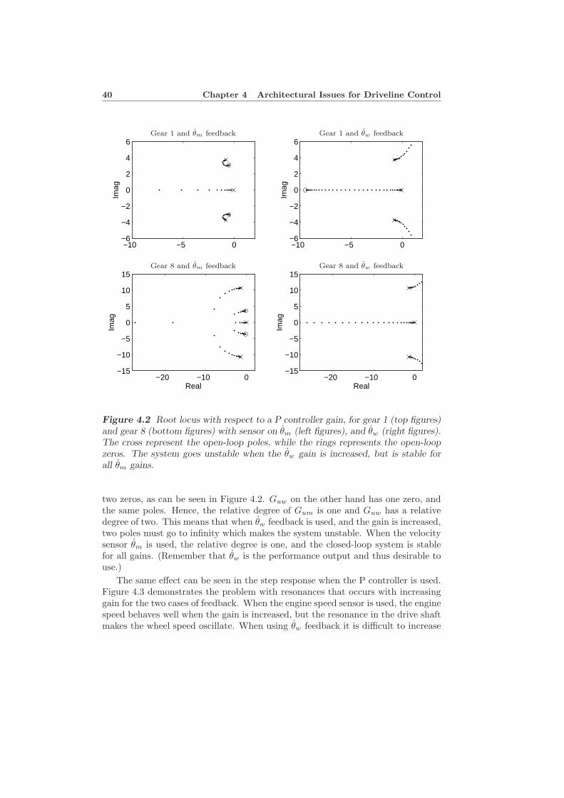
Figure 4.2 Root locus with respect to a P controller gain, for gear 1 (top figures)and gear 8 (bottom figures) with sensor on θm (left figures), and θw (right figures).The cross represent the open-loop poles, while the rings represents the open-loopzeros. The system goes unstable when the θw gain is increased, but is stable forall θm gains.
two zeros, as can be seen in Figure 4.2. Guw on the other hand has one zero, andthe same poles. Hence, the relative degree of Gum is one and Guw has a relativedegree of two. This means that when θw feedback is used, and the gain is increased,two poles must go to infinity which makes the system unstable. When the velocitysensor θm is used, the relative degree is one, and the closed-loop system is stablefor all gains. (Remember that θw is the performance output and thus desirable touse.)
The same effect can be seen in the step response when the P controller is used.Figure 4.3 demonstrates the problem with resonances that occurs with increasinggain for the two cases of feedback. When the engine speed sensor is used, the enginespeed behaves well when the gain is increased, but the resonance in the drive shaftmakes the wheel speed oscillate. When using θw feedback it is difficult to increase
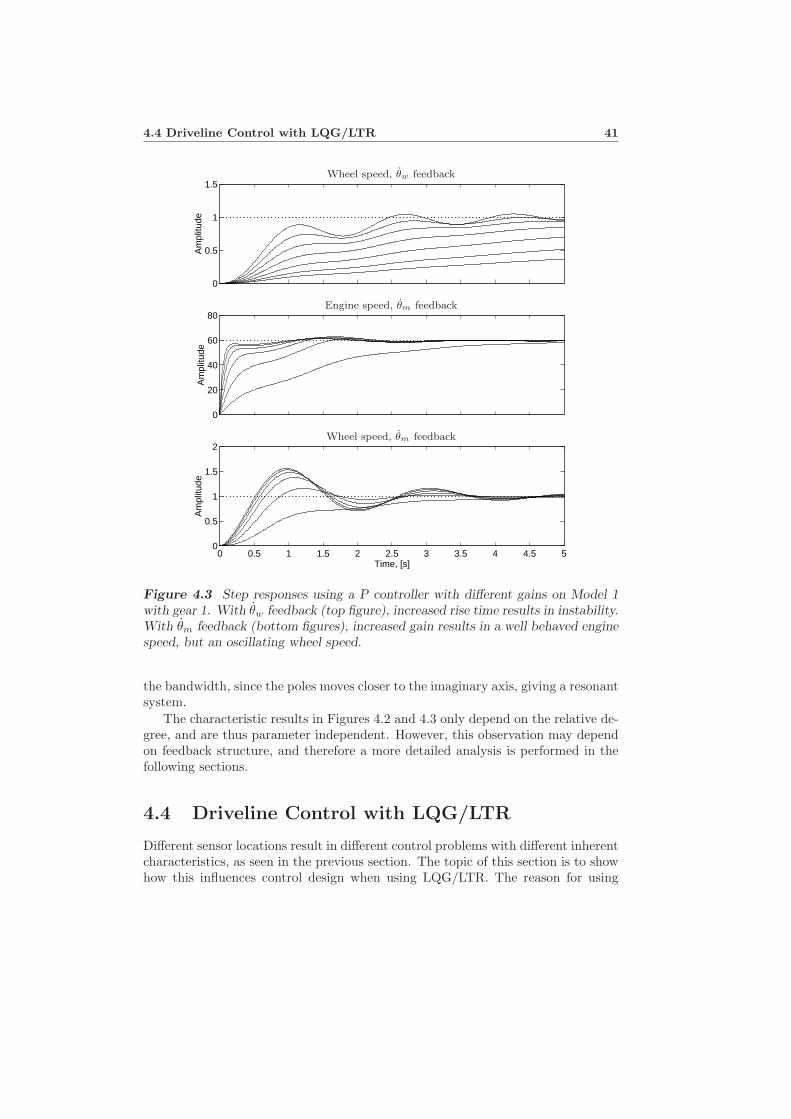
4.4 Driveline Control with LQG/LTR 41
0
0.5
1
1.5
Am
plitu
de
0
20
40
60
80
Am
plitu
de
0 0.5 1 1.5 2 2.5 3 3.5 4 4.5 50
0.5
1
1.5
2
Time, [s]
Am
plitu
de
Wheel speed, θw feedback
Engine speed, θm feedback
Wheel speed, θm feedback
Figure 4.3 Step responses using a P controller with different gains on Model 1with gear 1. With θw feedback (top figure), increased rise time results in instability.With θm feedback (bottom figures), increased gain results in a well behaved enginespeed, but an oscillating wheel speed.
the bandwidth, since the poles moves closer to the imaginary axis, giving a resonantsystem.
The characteristic results in Figures 4.2 and 4.3 only depend on the relative de-gree, and are thus parameter independent. However, this observation may dependon feedback structure, and therefore a more detailed analysis is performed in thefollowing sections.
4.4 Driveline Control with LQG/LTR
Different sensor locations result in different control problems with different inherentcharacteristics, as seen in the previous section. The topic of this section is to showhow this influences control design when using LQG/LTR. The reason for using
42 Chapter 4 Architectural Issues for Driveline Control
LQG/LTR, in this principle study, is that it offers a control design method resultingin a controller and observer of the same order as the plant model, and it is also aneasy method for obtaining robust controllers.
4.4.1 Transfer Functions
When comparing the control problem with using θm or θw as sensors, open-looptransfer functions Gum and Guw results. These have the same number of poles butdifferent number of zeros as mentioned before. Two different closed-loop systemsresults depending on which sensor that is used.
Feedback from θw
A natural feedback configuration is to use the performance output, θw. Thenamong others the following transfer functions results, where (4.16) to (4.21) areused together with the matrix inversion lemma
Grz =GuwFyFr
1 + GuwFy= TwFr (4.25)
Gnu = =1
1 + GuwFy= Sw (4.26)
where n is the input disturbance. The transfer functions Sw and Tw are, as usual,the sensitivity function and the complementary sensitivity function. Also, as usual,
Sw + Tw = 1 (4.27)
Feedback from θm
The following transfer functions results if the sensor measures θm
Grz =GuwFyFr
1 + GumFy(4.28)
Gnu =1
1 + GumFy(4.29)
The difference between the two feedback configurations is that the return differenceis 1 + GuwFy or 1 + GumFy.
It is desirable to have sensitivity functions that corresponds to y = θm andz = θw. The following transfer functions are defined
Sm =1
1 + GumFy, Tm =
GumFy
1 + GumFy(4.30)
These transfer functions corresponds to a configuration where θm is the output (i.e.y = z = θm). Using (4.28) it is natural to define Tm by
Tm =GuwFy
1 + GumFy= Tm
Guw
Gum(4.31)
4.4 Driveline Control with LQG/LTR 43
The functions Sm and Tm describe the design problem when feedback from θm isused.
When combining (4.30) and (4.31), the corresponding relation to (4.27) is
Sm + TmGum
Guw= 1 (4.32)
If Sm is made zero for some frequencies in (4.32), then Tm will not be equal toone, as in (4.27). Instead, Tm = Guw/Gum for these frequency domains.
Limitations on Performance
The relations (4.27) and (4.32) will be the fundamental relations for discussingdesign considerations. The impact of the ratio Guw/Gum will be analyzed in thefollowing sections.
Definition 4.1 Tm in (4.31) is the modified complementary sensitivity function,and Gw/m = Guw/Gum is the dynamic output ratio.
4.4.2 Design Example with a Simple Mass-Spring Model
Linear Quadratic Design with Loop Transfer Recovery will be treated in four cases,being combinations of two sensor locations, θm or θw, and two models with thesame structure, but with different parameters. Design without pre filter (Fr = 1)is considered.
The section covers a general plant with n inertias connected by k − 1 torsionalflexibilities, without damping and load, and with unit conversion ratio. There are(2n − 1) poles, and the location of the poles are the same for the different sensorlocations. The number of zeros depends on which sensor that is used, and whenusing θw there are no zeros. When using feedback from θm there are (2n−2) zeros.Thus, the transfer functions Gum and Guw, have the same denominators, and arelative degree of 1 and (2n − 1) respectively.
Structural Properties of Sensor Location
The controller (4.15) has a relative degree of one. The relative degree of GumFy isthus 2, and the relative degree of GuwFy is 2n. When considering design, a goodalternative is to have relative degree one in GFy, implying infinite gain margin andhigh phase margin.
When using GumFy, one pole has to be moved to infinity, and when usingGuwFy, 2n−1 poles have to be moved to infinity, in order for the ratio to resemblea first order system at high frequencies. It could be expected that a higher controlsignal is needed for θw feedback in order to move the poles towards infinity.
When the return ratio behaves like a first order system, also the closed-looptransfer function behaves like one. This conflicts with the design goal of having
44 Chapter 4 Architectural Issues for Driveline Control
10−1
100
101
102
−60
−50
−40
−30
−20
−10
0
10
Frequency (rads^−1)
Gai
n (
dB)
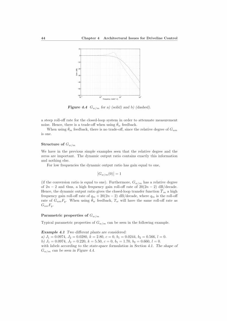
Figure 4.4 Gw/m for a) (solid) and b) (dashed).
a steep roll-off rate for the closed-loop system in order to attenuate measurementnoise. Hence, there is a trade-off when using θw feedback.
When using θm feedback, there is no trade-off, since the relative degree of Gum
is one.
Structure of Gw/m
We have in the previous simple examples seen that the relative degree and thezeros are important. The dynamic output ratio contains exactly this informationand nothing else.
For low frequencies the dynamic output ratio has gain equal to one,∣∣Gw/m(0)
∣∣ = 1
(if the conversion ratio is equal to one). Furthermore, Gw/m has a relative degreeof 2n − 2 and thus, a high frequency gain roll-off rate of 20(2n − 2) dB/decade.Hence, the dynamic output ratio gives the closed-loop transfer function Tm a highfrequency gain roll-off rate of qm + 20(2n − 2) dB/decade, where qm is the roll-offrate of GumFy. When using θw feedback, Tw will have the same roll-off rate asGuwFy.
Parametric properties of Gw/m
Typical parametric properties of Gw/m can be seen in the following example.
Example 4.1 Two different plants are considered:a) J1 = 0.0974, J2 = 0.0280, k = 2.80, c = 0, b1 = 0.0244, b2 = 0.566, l = 0.b) J1 = 0.0974, J2 = 0.220, k = 5.50, c = 0, b1 = 1.70, b2 = 0.660, l = 0.with labels according to the state-space formulation in Section 4.1. The shape ofGw/m can be seen in Figure 4.4.
4.4 Driveline Control with LQG/LTR 45
LQG Designs
Integral action is included by augmenting the state to attenuate step disturbancesin v (Maciejowski 1989). The state-space realization Aa, Ba, Ma, Cwa, and Cma re-sults. The Kalman-filter gain, Kf , is derived using a Riccati equation (Maciejowski1989)
PfAT + APf − PfCT V −1CPf + BWBT = 0 (4.33)
The covariances W and V , of v and e respectively, are adjusted until the returnratio
C(sI − A)−1Kf , Kf = PfCT V −1 (4.34)
and the closed-loop transfer functions S and T show satisfactory performance.The Nyquist locus remains outside the unit circle centered at −1. This means thatthere is infinite gain margin, and a phase margin of at least 60◦. Furthermore, therelative degree is one, and |S| ≤ 1.
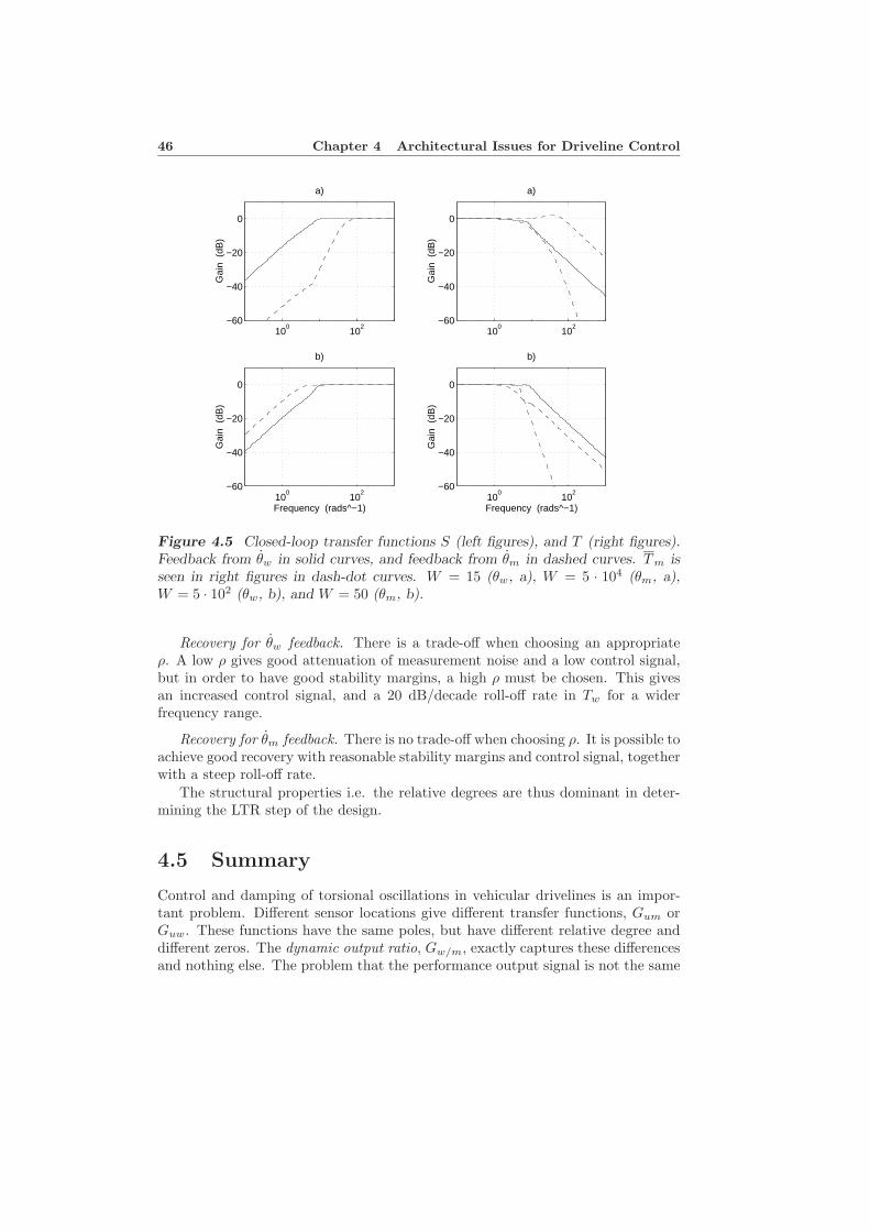
Design for θw feedback. W is adjusted (and thus Fy(s)) such that Sw and Tw
show a satisfactory performance, and that the desired bandwidth is obtained. Thedesign in Example 4 is shown in Figure 4.5. Note that the roll-off rate of Tw is 20dB/decade.
Design for θm feedback. W is adjusted (and thus Fy(s)) such that Sm and Tm
(and thus θm) show a satisfactory performance. Depending on the shape of Gw/m
for middle high frequencies, corrections in W must be taken such that Tm achievesthe desired bandwidth. If there is a resonance peak in Gw/m, the bandwidth inTm is chosen such that the peak is suppressed. Figure 4.5 shows such an example,θm feedback in b), where the bandwidth is lower in order to suppress the peak inGw/m. Note also the difference between Sw and Sm.
The parameters of the dynamic output ratio are thus important in the LQGstep of the design.
Loop Transfer Recovery, LTR
The next step in the design process is to include Kc, and recover the satisfactory re-turn ratio obtain previously. When using the combined state feedback and Kalmanfilter, the return ratio is GFy = C(sI − A)−1BKc(sI −A + BKc + KfC)−1Kf . Asimplistic LTR can be obtained by using Kc = ρC and increasing ρ. As ρ is in-creased, 2n − 1 poles move towards the open system zeros. The remaining polesmove towards infinity (compare to Section 5.1). If the Riccati equation
AT Pc + PcA − PcBR−1BT Pc + CT QC = 0 (4.35)
is solved with Q = ρ, and R = 1, Kc =√
ρC is obtained in the limit, and toguarantee stability, this Kc is used for recovery.
In Figures 4.6 and 4.7, the recovered closed-loop transfer functions, Nyquistlocus, and control signal are seen.
46 Chapter 4 Architectural Issues for Driveline Control
100
102
−60
−40
−20
0
Gai
n (
dB)
a)
100
102
−60
−40
−20
0G
ain
(dB
)
a)
100
102
−60
−40
−20
0
Frequency (rads^−1)
Gai
n (
dB)
b)
100
102
−60
−40
−20
0
Frequency (rads^−1)
Gai
n (
dB)
b)
Figure 4.5 Closed-loop transfer functions S (left figures), and T (right figures).Feedback from θw in solid curves, and feedback from θm in dashed curves. Tm isseen in right figures in dash-dot curves. W = 15 (θw, a), W = 5 · 104 (θm, a),W = 5 · 102 (θw, b), and W = 50 (θm, b).
Recovery for θw feedback. There is a trade-off when choosing an appropriateρ. A low ρ gives good attenuation of measurement noise and a low control signal,but in order to have good stability margins, a high ρ must be chosen. This givesan increased control signal, and a 20 dB/decade roll-off rate in Tw for a widerfrequency range.
Recovery for θm feedback. There is no trade-off when choosing ρ. It is possible toachieve good recovery with reasonable stability margins and control signal, togetherwith a steep roll-off rate.
The structural properties i.e. the relative degrees are thus dominant in deter-mining the LTR step of the design.
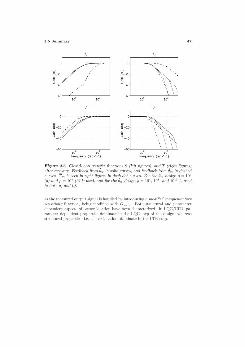
4.5 Summary
Control and damping of torsional oscillations in vehicular drivelines is an impor-tant problem. Different sensor locations give different transfer functions, Gum orGuw. These functions have the same poles, but have different relative degree anddifferent zeros. The dynamic output ratio, Gw/m, exactly captures these differencesand nothing else. The problem that the performance output signal is not the same
4.5 Summary 47
100
102
−60
−40
−20
0
Gai
n (
dB)
a)
100
102
−60
−40
−20
0
Gai
n (
dB)
a)
100
102
−60
−40
−20
0
Frequency (rads^−1)
Gai
n (
dB)
b)
100
102
−60
−40
−20
0
Frequency (rads^−1)
Gai
n (
dB)
b)
Figure 4.6 Closed-loop transfer functions S (left figures), and T (right figures)after recovery. Feedback from θw in solid curves, and feedback from θm in dashedcurves. Tm is seen in right figures in dash-dot curves. For the θm design ρ = 106
(a) and ρ = 105 (b) is used, and for the θw design ρ = 104, 108, and 1011 is usedin both a) and b).
as the measured output signal is handled by introducing a modified complementarysensitivity function, being modified with Gw/m. Both structural and parameterdependent aspects of sensor location have been characterized. In LQG/LTR, pa-rameter dependent properties dominate in the LQG step of the design, whereasstructural properties, i.e. sensor location, dominate in the LTR step.
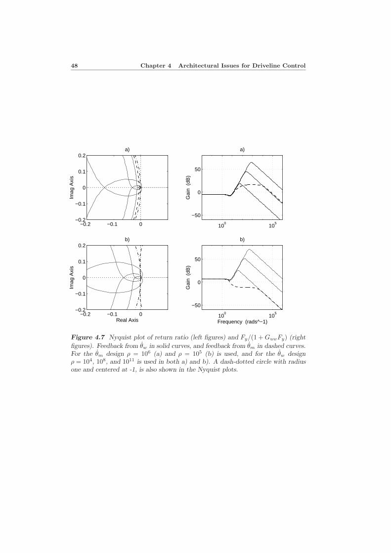
48 Chapter 4 Architectural Issues for Driveline Control
−0.2 −0.1 0−0.2
−0.1
0
0.1
0.2
Imag
Axi
s
a)
100
105
−50
0
50
Gai
n (
dB)
a)
−0.2 −0.1 0−0.2
−0.1
0
0.1
0.2
Real Axis
Imag
Axi
s
b)
100
105
−50
0
50
Frequency (rads^−1)
Gai
n (
dB)
b)
Figure 4.7 Nyquist plot of return ratio (left figures) and Fy/(1 + GuwFy) (right
figures). Feedback from θw in solid curves, and feedback from θm in dashed curves.For the θm design ρ = 106 (a) and ρ = 105 (b) is used, and for the θw designρ = 104, 108, and 1011 is used in both a) and b). A dash-dotted circle with radiusone and centered at -1, is also shown in the Nyquist plots.
5Speed Controller Design and
Simulations
Driveline oscillations may occur in different modes of operation. Active dampingin two modes will be treated in this and next chapter. The first problem is wheelspeed oscillations following a change in accelerator pedal position, known as vehicleshuffle (Mo, Beaumount, and Powell 1996; Pettersson and Nielsen 1995). Tradi-tionally in diesel powered trucks, the relation between the accelerator pedal andthe amount of fuel metered by the diesel pump is governed by a system called RQVcontrol. The RQV control gives a specific character to the driving feeling e.g. whengoing uphill and downhill. This driving character is important to maintain whenextending speed control with active damping. Traditional RQV control is explainedin Section 5.1. Thereafter, the speed control problem keeping RQV characteristicsis formulated in Section 5.2. The sections following study the problem using avail-able computationally powerful methods like LQG/LTR. Sensor location, influencefrom disturbances, and load estimations are treated.
5.1 RQV Control
RQV control is the traditional diesel engine control scheme steaming from themechanical centrifugal governor, used to control the diesel pump (Bosch 1993). Intodays electronically controlled engines, the RQV scheme is still used for controllingthe fuel amount to the engine, since the driver wants the engine to behave as withthe mechanical governor.
RQV control is essentially a P controller with the accelerator as reference valueand a sensor measuring the engine speed. The RQV controller has no informationabout the load, and a nonzero load (e.g. going uphill or downhill) gives a stationary
49
50 Chapter 5 Speed Controller Design and Simulations
error. The RQV controller is described by
u = u0 + Kp(ri − θm) (5.1)
where i = itif is the conversion ratio of the driveline, Kp is the controller gain, andr is the reference velocity. The constant u0 is a function of the speed, but not theload since this is unknown to the RQV controller. RQV control is demonstrated inthe following example.
Example 5.1 Consider the truck modeled in Chapters 2 and 3 traveling at a speedof 2 rad/s (3.6 km/h) with gear 1 and a total load of 3000 Nm (≈ 2 % road slope).Let the new desired velocity be r = 2.3 rad/s. Figure 5.1 shows the RQV controllaw (5.1) applied to Model 1 with three gains Kp. In the plots, u0 is calculatedsuch that the stationary level is the same for the three gains. (Otherwise therewould be a gain dependent stationary error.)
When the controller gain is increased, the rise time and the overshoot is in-creasing. Hence, there is a trade-off between short rise time and little overshoot.Furthermore, the engine speed behaves well, but the flexibility of the drivelinecauses the wheel speed to oscillate, when the gain is increased.
Figure 5.2 shows the transfer functions from load and measurement disturbancesv and e to the performance output, when the RQV controller is used. The resonancepeak in the transfer functions is increasing when the controller gain is increased.
5.2 Problem Formulation
The performance output for the speed controller is the wheel speed, z = θw, asdefined in Chapter 4. In Figure 5.3, the wheel speed z is seen for Models 1 and2. Model 2 adds a second resonance peak from the clutch. Furthermore, the highfrequency roll-off rate is steeper for Model 2 than for Model 1. Note that thetransfer function from the load l to the performance output z is the same for thetwo models. This chapter deals with the development of a controller based onModel 1.
5.2.1 Mathematical Problem Formulation
A first possible attempt for speed control is a scheme of applying the engine torqueto the driveline such that the following cost function is minimized
limT→∞
∫ T
0
(z − r)2 (5.2)
where r is the reference velocity given by the driver. If a control law is to minimizethe cost function, then (5.2) can be made arbitrarily small if there are no restrictionson the control signal u, since the plant model is linear. A diesel engine can onlyproduce torque in a certain range, and therefore, (5.2) is extended such that a largecontrol signal adds to the cost function.
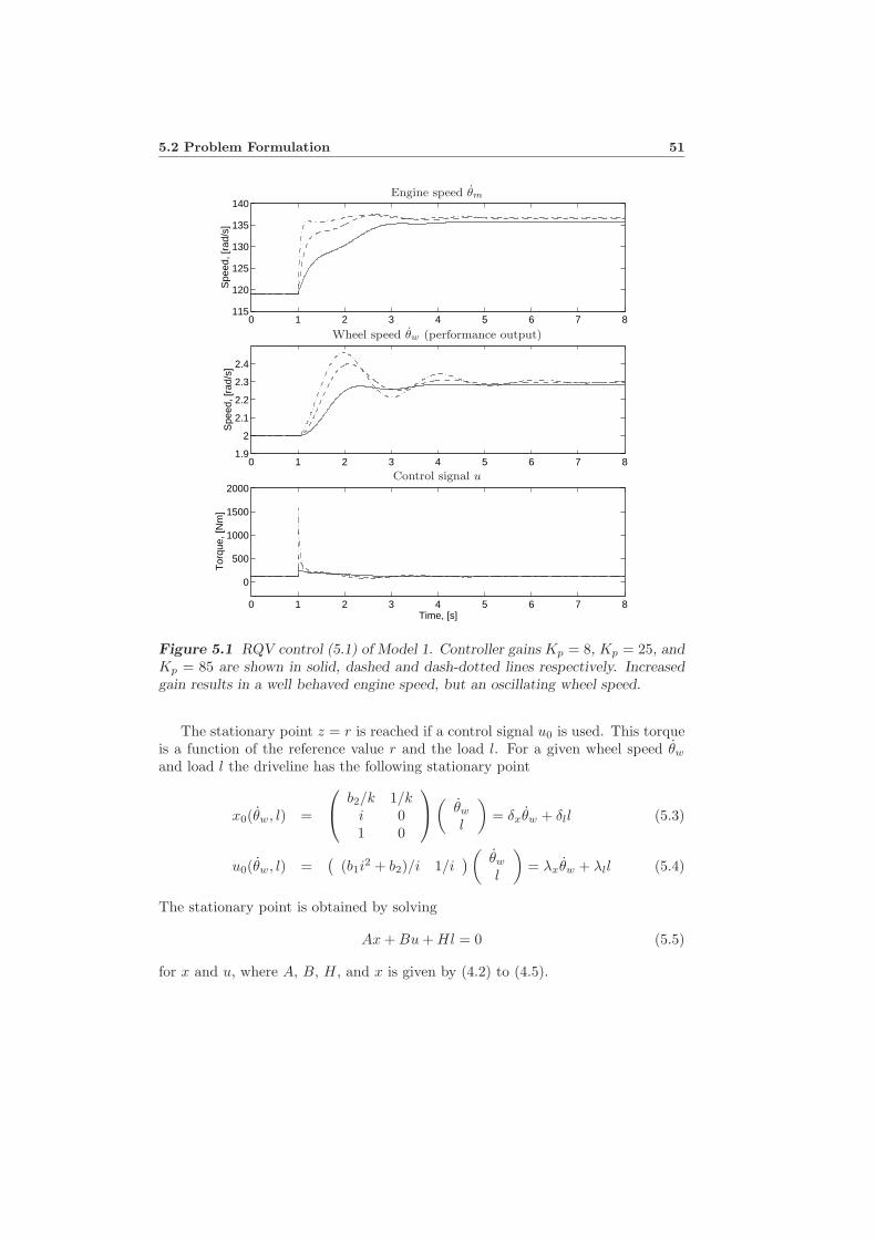
5.2 Problem Formulation 51
0 1 2 3 4 5 6 7 8115
120
125
130
135
140
Spe
ed, [
rad/
s]
0 1 2 3 4 5 6 7 81.9
2
2.1
2.2
2.3
2.4
Spe
ed, [
rad/
s]
0 1 2 3 4 5 6 7 8
0
500
1000
1500
2000
Time, [s]
Tor
que,
[Nm
]
Engine speed θm
Wheel speed θw (performance output)
Control signal u
Figure 5.1 RQV control (5.1) of Model 1. Controller gains Kp = 8, Kp = 25, andKp = 85 are shown in solid, dashed and dash-dotted lines respectively. Increasedgain results in a well behaved engine speed, but an oscillating wheel speed.
The stationary point z = r is reached if a control signal u0 is used. This torqueis a function of the reference value r and the load l. For a given wheel speed θw
and load l the driveline has the following stationary point
x0(θw, l) =
b2/k 1/k
i 01 0
(
θw
l
)= δxθw + δll (5.3)
u0(θw, l) =(
(b1i2 + b2)/i 1/i
) (θw
l
)= λxθw + λll (5.4)
The stationary point is obtained by solving
Ax + Bu + Hl = 0 (5.5)
for x and u, where A, B, H, and x is given by (4.2) to (4.5).
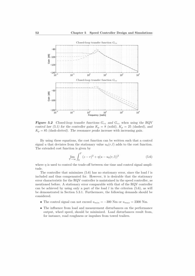
52 Chapter 5 Speed Controller Design and Simulations
10−2
10−1
100
101
102
103
−140
−120
−100
−80
Gai
n [d
B]
10−2
10−1
100
101
102
103
−150
−100
−50
Frequency [rad/s]
Gai
n [d
B]
Closed-loop transfer function Gvz
Closed-loop transfer function Gez
Figure 5.2 Closed-loop transfer functions Gvz and Gez when using the RQVcontrol law (5.1) for the controller gains Kp = 8 (solid), Kp = 25 (dashed), andKp = 85 (dash-dotted). The resonance peaks increase with increasing gain.
By using these equations, the cost function can be written such that a controlsignal u that deviates from the stationary value u0(r, l) adds to the cost function.The extended cost function is given by
limT→∞
∫ T
0
(z − r)2 + η(u − u0(r, l))2 (5.6)
where η is used to control the trade-off between rise time and control signal ampli-tude.
The controller that minimizes (5.6) has no stationary error, since the load l isincluded and thus compensated for. However, it is desirable that the stationaryerror characteristic for the RQV controller is maintained in the speed controller, asmentioned before. A stationary error comparable with that of the RQV controllercan be achieved by using only a part of the load l in the criterion (5.6), as willbe demonstrated in Section 5.3.1. Furthermore, the following demands should beconsidered.
• The control signal can not exceed umin = −300 Nm or umax = 2300 Nm.
• The influence from load and measurement disturbances on the performanceoutput, wheel speed, should be minimized. Load disturbances result from,for instance, road roughness or impulses from towed trailers.
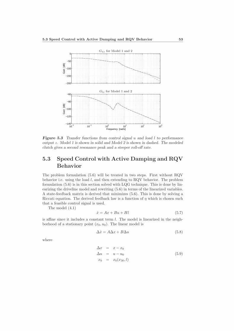
5.3 Speed Control with Active Damping and RQV Behavior 53
−200
−150
−100
−50
0
Gai
n [d
B]
10−2
10−1
100
101
102
103
−140
−120
−100
−80
−60
Frequency [rad/s]
Gai
n [d
B]
Guz for Model 1 and 2
Glz for Model 1 and 2
Figure 5.3 Transfer functions from control signal u and load l to performanceoutput z. Model 1 is shown in solid and Model 2 is shown in dashed. The modeledclutch gives a second resonance peak and a steeper roll-off rate.
5.3 Speed Control with Active Damping and RQVBehavior
The problem formulation (5.6) will be treated in two steps. First without RQVbehavior i.e. using the load l, and then extending to RQV behavior. The problemformulation (5.6) is in this section solved with LQG technique. This is done by lin-earizing the driveline model and rewriting (5.6) in terms of the linearized variables.A state-feedback matrix is derived that minimizes (5.6). This is done by solving aRiccati equation. The derived feedback law is a function of η which is chosen suchthat a feasible control signal is used.
The model (4.1)x = Ax + Bu + Hl (5.7)
is affine since it includes a constant term l. The model is linearized in the neigh-borhood of a stationary point (x0, u0). The linear model is
∆x = A∆x + B∆u (5.8)
where
∆x = x − x0
∆u = u − u0 (5.9)x0 = x0(x30, l)
54 Chapter 5 Speed Controller Design and Simulations
u0 = u0(x30, l)
where the stationary point (x0, u0) is given by (5.3) and (5.4). Note that the linearmodel is the same for all stationary points.
The problem is to devise a feedback-control law that minimizes the cost function(5.6). The cost function is expressed in terms of ∆x and ∆u by using (5.9)
limT→∞
∫ T
0
(M(x0 + ∆x) − r)2 + η(u0 + ∆u − u0(r, l))2 (5.10)
= limT→∞
∫ T
0
(M∆x + r1)2 + η(∆u + r2)2 (5.11)
with
r1 = Mx0 − r (5.12)r2 = u0 − u0(r, l)
In order to minimize (5.10) a Riccati equation is solved. Then the constants r1 andr2 must be expressed in terms of state variables. This can be done by augmentingthe plant model (A, B) with models of the constants r1 and r2. Since these modelswill not be controllable, they must be stable in order to solve the Riccati equation(Maciejowski 1989). Therefore the model r1 = r2 = 0 cannot be used because thepoles are located on the imaginary axis. Instead the following are used
r1 = −αr1 (5.13)r2 = −αr2 (5.14)
which with a low α indicates that r is a slow varying constant.The augmented model is given by
Ar =
0 0A 0 0
0 0−α 0
0 0 0 0 −α
, (5.15)
Br =
B
00
, xr = (∆xT r1 r2)T (5.16)
By using these equations, the cost function (5.10) can be written in the form
limT→∞
∫ T
0
xTr Qxr + R∆u2 + 2xT
r N∆u (5.17)
with
Q = (M 1 0)T (M 1 0) + η(0 0 0 0 1)T (0 0 0 0 1)N = η(0 0 0 0 1)T (5.18)R = η
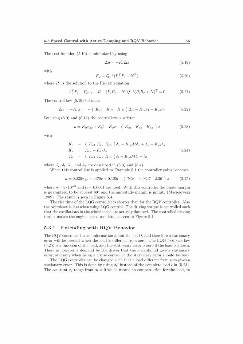
5.3 Speed Control with Active Damping and RQV Behavior 55
The cost function (5.10) is minimized by using
∆u = −Kc∆x (5.19)
withKc = Q−1(BT
r Pc + NT ) (5.20)
where Pc is the solution to the Riccati equation
ATr Pc + PcAr + R − (PcBr + N)Q−1(PcBr + N)T = 0 (5.21)
The control law (5.19) becomes
∆u = −Kcxr = − (Kc1 Kc2 Kc3
)∆x − Kc4r1 − Kc5r2 (5.22)
By using (5.9) and (5.12) the control law is written
u = K0x30 + Kll + Krr −(
Kc1 Kc2 Kc3
)x (5.23)
with
K0 =(
Kc1 Kc2 Kc3
)δx − Kc4Mδx + λx − Kc5λx
Kr = Kc4 + Kc5λx (5.24)Kl =
(Kc1 Kc2 Kc3
)δl − Kc4Mδl + λl
where δx, δl, λx, and λl are described in (5.3) and (5.4).When this control law is applied to Example 5.1 the controller gains becomes
u = 0.230x30 + 4470r + 0.125l − (7620 0.0347 2.36
)x (5.25)
where η = 5 · 10−8 and α = 0.0001 are used. With this controller the phase marginis guaranteed to be at least 60◦ and the amplitude margin is infinity (Maciejowski1989). The result is seen in Figure 5.4.
The rise time of the LQG controller is shorter than for the RQV controller. Alsothe overshoot is less when using LQG control. The driving torque is controlled suchthat the oscillations in the wheel speed are actively damped. The controlled drivingtorque makes the engine speed oscillate, as seen in Figure 5.4.
5.3.1 Extending with RQV Behavior
The RQV controller has no information about the load l, and therefore a stationaryerror will be present when the load is different from zero. The LQG feedback law(5.25) is a function of the load, and the stationary error is zero if the load is known.There is however a demand by the driver that the load should give a stationaryerror, and only when using a cruise controller the stationary error should be zero.
The LQG controller can be changed such that a load different from zero gives astationary error. This is done by using βll instead of the complete load l in (5.23).The constant βl range from βl = 0 which means no compensation for the load, to
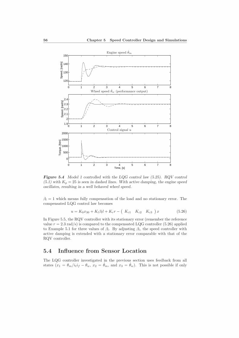
56 Chapter 5 Speed Controller Design and Simulations
0 1 2 3 4 5 6 7 8
120
130
140
150
Spe
ed, [
rad/
s]
0 1 2 3 4 5 6 7 81.9
2
2.1
2.2
2.3
2.4
Spe
ed, [
rad/
s]
0 1 2 3 4 5 6 7 8
0
500
1000
1500
2000
Time, [s]
Tor
que,
[Nm
]
Engine speed θm
Wheel speed θw (performance output)
Control signal u
Figure 5.4 Model 1 controlled with the LQG control law (5.25). RQV control(5.1) with Kp = 25 is seen in dashed lines. With active damping, the engine speedoscillates, resulting in a well behaved wheel speed.
βl = 1 which means fully compensation of the load and no stationary error. Thecompensated LQG control law becomes
u = K0x30 + Klβll + Krr −(
Kc1 Kc2 Kc3
)x (5.26)
In Figure 5.5, the RQV controller with its stationary error (remember the referencevalue r = 2.3 rad/s) is compared to the compensated LQG controller (5.26) appliedto Example 5.1 for three values of βl. By adjusting βl, the speed controller withactive damping is extended with a stationary error comparable with that of theRQV controller.
5.4 Influence from Sensor Location
The LQG controller investigated in the previous section uses feedback from allstates (x1 = θm/itif − θw, x2 = θm, and x3 = θw). This is not possible if only
5.4 Influence from Sensor Location 57
0 1 2 3 4 5 6 7 81.95
2
2.05
2.1
2.15
2.2
2.25
2.3
2.35
Time, [s]
Spe
ed, [
rad/
s]
Figure 5.5 Example 5.1 controlled with the RQV controller (5.1) in dashed line,and the LQG controller with stationary error (5.26) with βl = 0, 0.5, 1. The LQGcontroller achieves the same stationary as the RQV controller by adjusting βl.
one sensor is used, which is the case considered in this work. The sensor eithermeasures the engine speed θm or the wheel speed θw. In this section an observeris used to estimate the rest of the states. The observer gain is calculated usingLTR technique. Then two different observer problems results depending on whichsensor location that is used.
The LQG feedback law (5.23) then becomes
u = K0x30 + Krr + Kll −(
Kc1 Kc2 Kc3
)x (5.27)
with K0, Kr, and Kl given by (5.24). The estimated states x are given by theKalman filter
∆ ˙x = A∆x + B∆u + Kf (∆y − C∆x) (5.28)Kf = PfCT V −1 (5.29)
where Pf is found by solving the Riccati equation
PfAT + APf − PfCT V −1CPf + W = 0 (5.30)
The covariance matrices W and V corresponds to v and e respectively. The outputmatrix C is either equal to Cm (4.11) when measuring the engine speed, or Cw
(4.12) when measuring the wheel speed.
58 Chapter 5 Speed Controller Design and Simulations
Loop-Transfer Recovery (LTR) is used to recover the properties achieved in theprevious design step when all states are measured. This is done by selecting
V = 1W = ρBBT (5.31)C = Cm or Cw
ρ = ρm or ρw
and solving (5.29) and (5.30) for Kf .When using LQG with feedback from all states, the phase margin ϕ is at least
60◦ and the amplitude margin a is infinity as stated before. This is obtained alsowhen using the observer by increasing ρ towards infinity. For Example 5.1 thefollowing values are used
ρm = 5 · 105 ⇒ ϕm = 60.5◦, am = ∞ (5.32)ρw = 1014 ⇒ ϕw = 59.9◦, aw = 35.0 (5.33)
where the aim has been to have at least 60◦ phase margin.The observer dynamics is cancelled in the transfer function from reference value
to performance output and control signal. Hence, these transfer functions are notaffected by the sensor location. However, the observer dynamics will be includedin the transfer functions from disturbances both to z and u.
5.4.1 Influence from Load Disturbances
Figure 5.6 shows how the performance output and the control signal are affectedby the load disturbance v. There is a resonance peak in Gvz when using feedbackfrom the engine speed sensor, which is not present when feedback from the wheelspeed sensor is used. The reason to this can be seen when studying the transferfunction Gvz in (4.20). By using the matrix inversion lemma (4.20) is rewritten as
(Gvz)cl =Gvz + Fy(GuyGvz − GuzGvy)
1 + GuyFy(5.34)
where Gab means the transfer function from signal a to b, and cl stands for closedloop. The signal y in (5.34) mean the output of the system, i.e. either θw or θm.The controller Fy is given by (4.15) as
Fy(s) = Kc(sI − A + BKc + KfC)−1Kf (5.35)
with C either as Cm for engine speed feedback, or Cw for wheel speed feedback.For the speed controller (z = θw), Equation (5.34) becomes
(Gvz)cl =Gvw
1 + GuwFy(5.36)
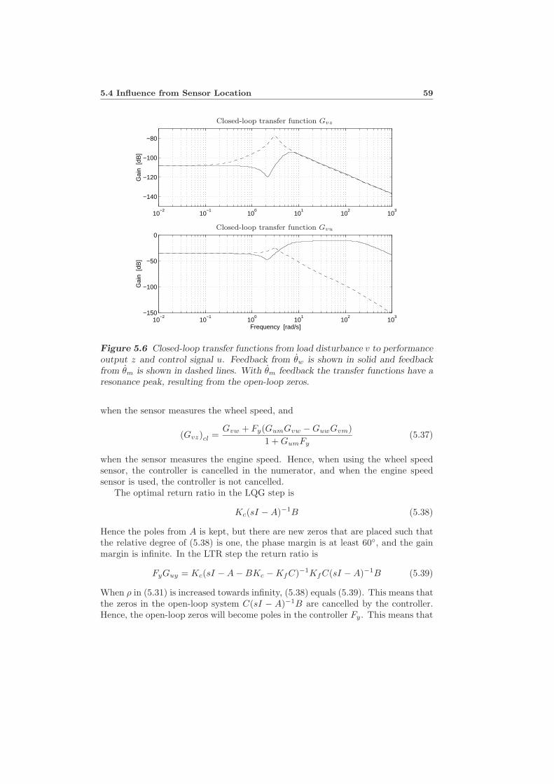
5.4 Influence from Sensor Location 59
10−2
10−1
100
101
102
103
−140
−120
−100
−80
Gai
n [d
B]
10−2
10−1
100
101
102
103
−150
−100
−50
0
Frequency [rad/s]
Gai
n [d
B]
Closed-loop transfer function Gvz
Closed-loop transfer function Gvu
Figure 5.6 Closed-loop transfer functions from load disturbance v to performanceoutput z and control signal u. Feedback from θw is shown in solid and feedbackfrom θm is shown in dashed lines. With θm feedback the transfer functions have aresonance peak, resulting from the open-loop zeros.
when the sensor measures the wheel speed, and
(Gvz)cl =Gvw + Fy(GumGvw − GuwGvm)
1 + GumFy(5.37)
when the sensor measures the engine speed. Hence, when using the wheel speedsensor, the controller is cancelled in the numerator, and when the engine speedsensor is used, the controller is not cancelled.
The optimal return ratio in the LQG step is
Kc(sI − A)−1B (5.38)
Hence the poles from A is kept, but there are new zeros that are placed such thatthe relative degree of (5.38) is one, the phase margin is at least 60◦, and the gainmargin is infinite. In the LTR step the return ratio is
FyGuy = Kc(sI − A − BKc − KfC)−1KfC(sI − A)−1B (5.39)
When ρ in (5.31) is increased towards infinity, (5.38) equals (5.39). This means thatthe zeros in the open-loop system C(sI − A)−1B are cancelled by the controller.Hence, the open-loop zeros will become poles in the controller Fy. This means that
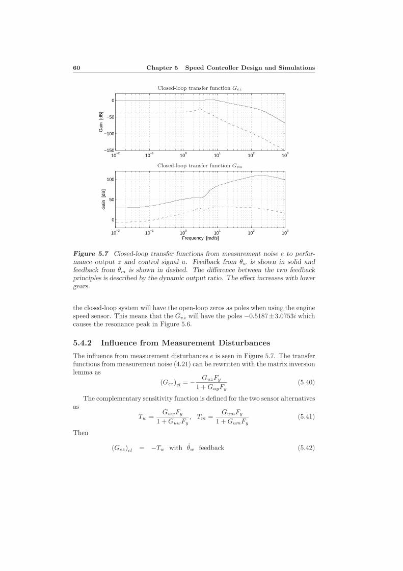
60 Chapter 5 Speed Controller Design and Simulations
10−2
10−1
100
101
102
103
−150
−100
−50
0
Gai
n [d
B]
10−2
10−1
100
101
102
103
0
50
100
Frequency [rad/s]
Gai
n [d
B]
Closed-loop transfer function Gez
Closed-loop transfer function Geu
Figure 5.7 Closed-loop transfer functions from measurement noise e to perfor-mance output z and control signal u. Feedback from θw is shown in solid andfeedback from θm is shown in dashed. The difference between the two feedbackprinciples is described by the dynamic output ratio. The effect increases with lowergears.
the closed-loop system will have the open-loop zeros as poles when using the enginespeed sensor. This means that the Gvz will have the poles −0.5187±3.0753i whichcauses the resonance peak in Figure 5.6.
5.4.2 Influence from Measurement Disturbances
The influence from measurement disturbances e is seen in Figure 5.7. The transferfunctions from measurement noise (4.21) can be rewritten with the matrix inversionlemma as
(Gez)cl = − GuzFy
1 + GuyFy(5.40)
The complementary sensitivity function is defined for the two sensor alternativesas
Tw =GuwFy
1 + GuwFy, Tm =
GumFy
1 + GumFy(5.41)
Then
(Gez)cl = −Tw with θw feedback (5.42)
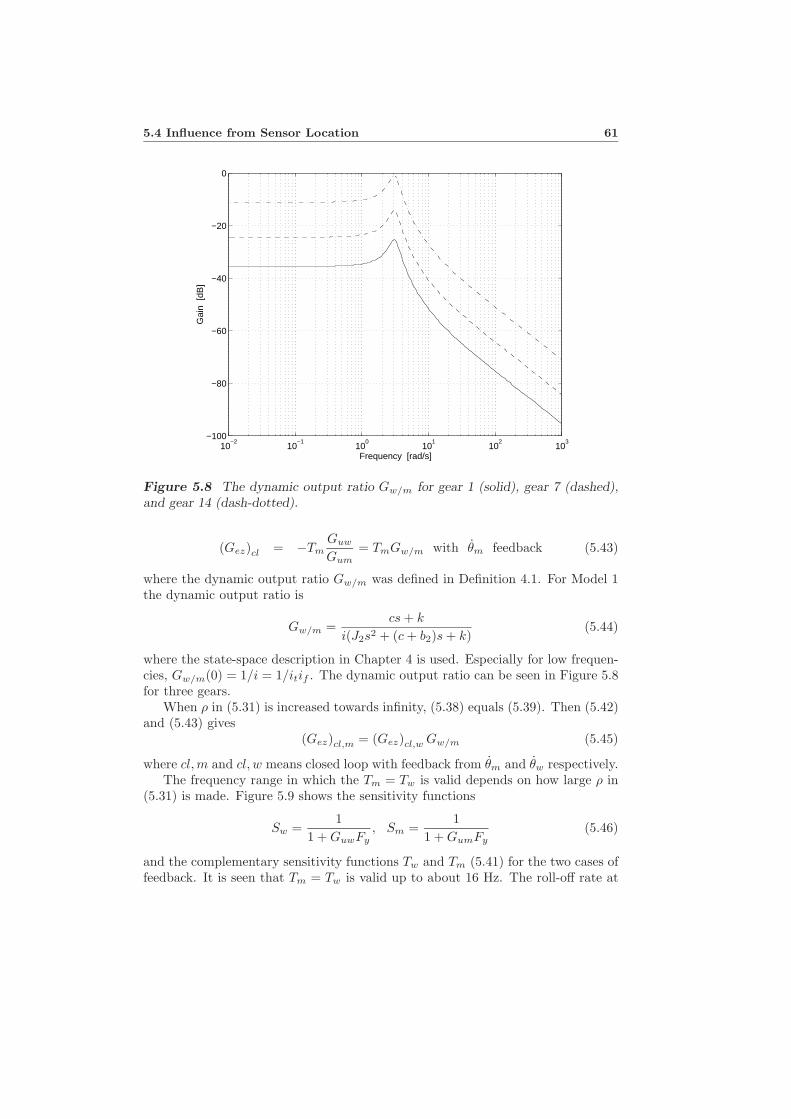
5.4 Influence from Sensor Location 61
10−2
10−1
100
101
102
103
−100
−80
−60
−40
−20
0
Frequency [rad/s]
Gai
n [d
B]
Figure 5.8 The dynamic output ratio Gw/m for gear 1 (solid), gear 7 (dashed),and gear 14 (dash-dotted).
(Gez)cl = −TmGuw
Gum= TmGw/m with θm feedback (5.43)
where the dynamic output ratio Gw/m was defined in Definition 4.1. For Model 1the dynamic output ratio is
Gw/m =cs + k
i(J2s2 + (c + b2)s + k)(5.44)
where the state-space description in Chapter 4 is used. Especially for low frequen-cies, Gw/m(0) = 1/i = 1/itif . The dynamic output ratio can be seen in Figure 5.8for three gears.
When ρ in (5.31) is increased towards infinity, (5.38) equals (5.39). Then (5.42)and (5.43) gives
(Gez)cl,m = (Gez)cl,w Gw/m (5.45)
where cl,m and cl, w means closed loop with feedback from θm and θw respectively.The frequency range in which the Tm = Tw is valid depends on how large ρ in
(5.31) is made. Figure 5.9 shows the sensitivity functions
Sw =1
1 + GuwFy, Sm =
11 + GumFy
(5.46)
and the complementary sensitivity functions Tw and Tm (5.41) for the two cases offeedback. It is seen that Tm = Tw is valid up to about 16 Hz. The roll-off rate at
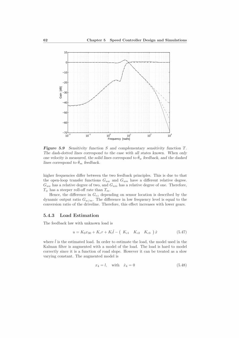
62 Chapter 5 Speed Controller Design and Simulations
10−2
10−1
100
101
102
103
−70
−60
−50
−40
−30
−20
−10
0
10
Frequency [rad/s]
Gai
n [d
B]
Figure 5.9 Sensitivity function S and complementary sensitivity function T .The dash-dotted lines correspond to the case with all states known. When onlyone velocity is measured, the solid lines correspond to θw feedback, and the dashedlines correspond to θm feedback.
higher frequencies differ between the two feedback principles. This is due to thatthe open-loop transfer functions Guw and Gum have a different relative degree.Guw has a relative degree of two, and Gum has a relative degree of one. Therefore,Tw has a steeper roll-off rate than Tm.
Hence, the difference in Gez depending on sensor location is described by thedynamic output ratio Gw/m. The difference in low frequency level is equal to theconversion ratio of the driveline. Therefore, this effect increases with lower gears.
5.4.3 Load Estimation
The feedback law with unknown load is
u = K0x30 + Krr + Kl l −(
Kc1 Kc2 Kc3
)x (5.47)
where l is the estimated load. In order to estimate the load, the model used in theKalman filter is augmented with a model of the load. The load is hard to modelcorrectly since it is a function of road slope. However it can be treated as a slowvarying constant. The augmented model is
x4 = l, with x4 = 0 (5.48)
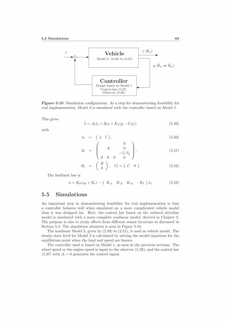
5.5 Simulations 63
ControllerDesign based on Model 1
Control law (5.27)Observer (5.28)
z (θw)
y (θw or θm)
r VehicleModel 3: (2.49) to (2.51)
Figure 5.10 Simulation configuration. As a step for demonstrating feasibility forreal implementation, Model 3 is simulated with the controller based on Model 1.
This gives˙x = Alxl + Blu + Kf (y − Clxl) (5.49)
with
xl =(
x l), (5.50)
Al =
0A 0
−1/J2
0 0 0 0
, (5.51)
Bl =(
B0
), Cl =
(C 0
)(5.52)
The feedback law is
u = K0x30 + Krr −(
Kc1 Kc2 Kc3 −Kl
)xl (5.53)
5.5 Simulations
An important step in demonstrating feasibility for real implementation is thata controller behaves well when simulated on a more complicated vehicle modelthan it was designed for. Here, the control law based on the reduced drivelinemodel is simulated with a more complete nonlinear model, derived in Chapter 2.The purpose is also to study effects from different sensor locations as discussed inSection 5.4. The simulation situation is seen in Figure 5.10.
The nonlinear Model 3, given by (2.49) to (2.51), is used as vehicle model. Thesteady-state level for Model 3 is calculated by solving the model equations for theequilibrium point when the load and speed are known.
The controller used is based on Model 1, as seen in the previous sections. Thewheel speed or the engine speed is input to the observer (5.28), and the control law(5.27) with βl = 0 generates the control signal.
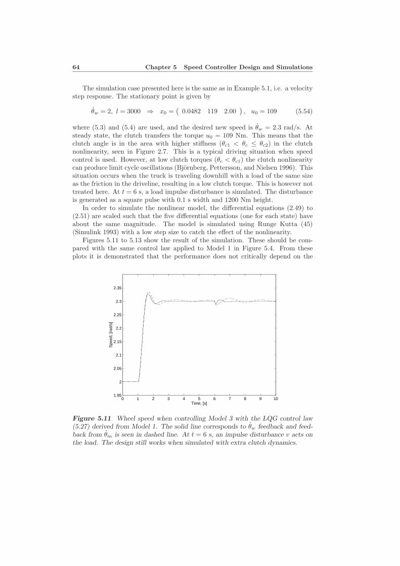
64 Chapter 5 Speed Controller Design and Simulations
The simulation case presented here is the same as in Example 5.1, i.e. a velocitystep response. The stationary point is given by
θw = 2, l = 3000 ⇒ x0 =(
0.0482 119 2.00), u0 = 109 (5.54)
where (5.3) and (5.4) are used, and the desired new speed is θw = 2.3 rad/s. Atsteady state, the clutch transfers the torque u0 = 109 Nm. This means that theclutch angle is in the area with higher stiffness (θc1 < θc ≤ θc2) in the clutchnonlinearity, seen in Figure 2.7. This is a typical driving situation when speedcontrol is used. However, at low clutch torques (θc < θc1) the clutch nonlinearitycan produce limit cycle oscillations (Bjornberg, Pettersson, and Nielsen 1996). Thissituation occurs when the truck is traveling downhill with a load of the same sizeas the friction in the driveline, resulting in a low clutch torque. This is however nottreated here. At t = 6 s, a load impulse disturbance is simulated. The disturbanceis generated as a square pulse with 0.1 s width and 1200 Nm height.
In order to simulate the nonlinear model, the differential equations (2.49) to(2.51) are scaled such that the five differential equations (one for each state) haveabout the same magnitude. The model is simulated using Runge Kutta (45)(Simulink 1993) with a low step size to catch the effect of the nonlinearity.
Figures 5.11 to 5.13 show the result of the simulation. These should be com-pared with the same control law applied to Model 1 in Figure 5.4. From theseplots it is demonstrated that the performance does not critically depend on the
0 1 2 3 4 5 6 7 8 9 101.95
2
2.05
2.1
2.15
2.2
2.25
2.3
2.35
Time, [s]
Spe
ed, [
rad/
s]
Figure 5.11 Wheel speed when controlling Model 3 with the LQG control law(5.27) derived from Model 1. The solid line corresponds to θw feedback and feed-back from θm is seen in dashed line. At t = 6 s, an impulse disturbance v acts onthe load. The design still works when simulated with extra clutch dynamics.
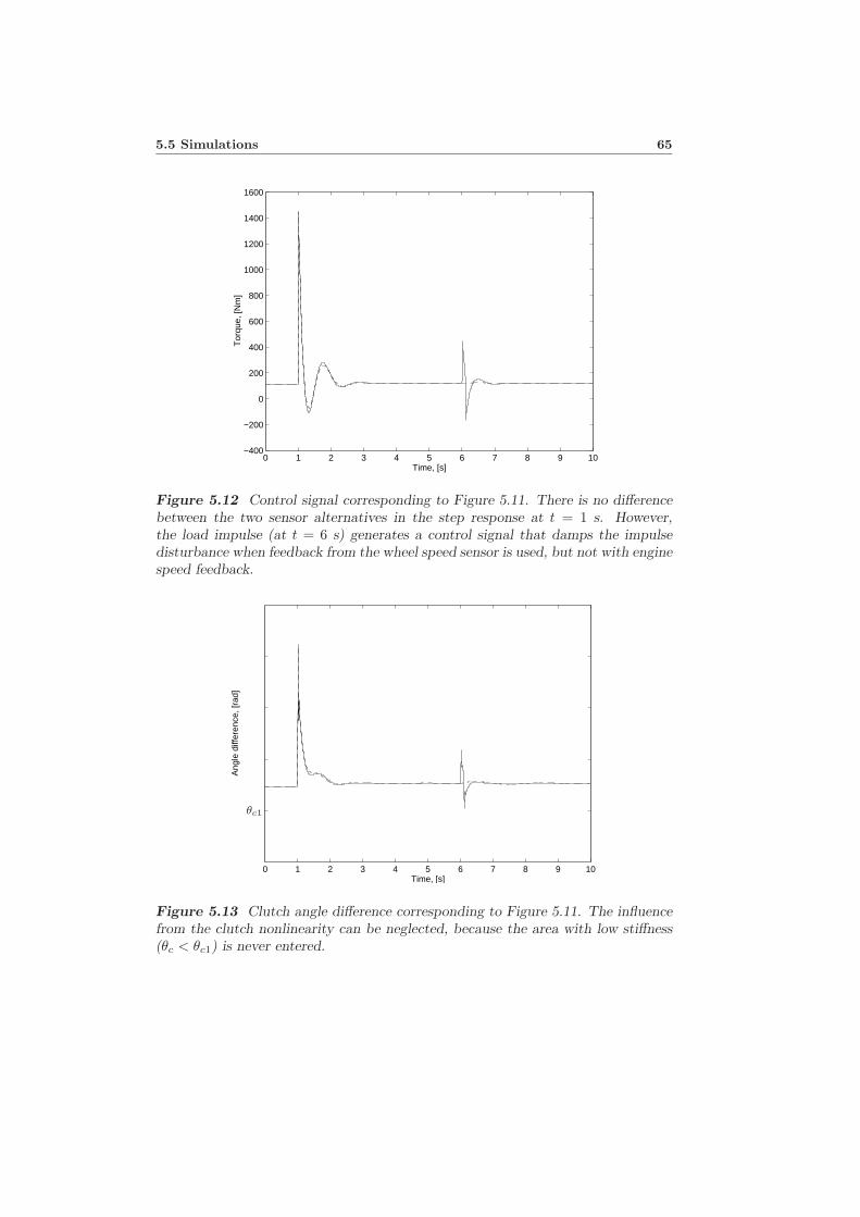
5.5 Simulations 65
0 1 2 3 4 5 6 7 8 9 10−400
−200
0
200
400
600
800
1000
1200
1400
1600
Time, [s]
Tor
que,
[Nm
]
Figure 5.12 Control signal corresponding to Figure 5.11. There is no differencebetween the two sensor alternatives in the step response at t = 1 s. However,the load impulse (at t = 6 s) generates a control signal that damps the impulsedisturbance when feedback from the wheel speed sensor is used, but not with enginespeed feedback.
0 1 2 3 4 5 6 7 8 9 10Time, [s]
Ang
le d
iffer
ence
, [ra
d]
θc1
Figure 5.13 Clutch angle difference corresponding to Figure 5.11. The influencefrom the clutch nonlinearity can be neglected, because the area with low stiffness(θc < θc1) is never entered.
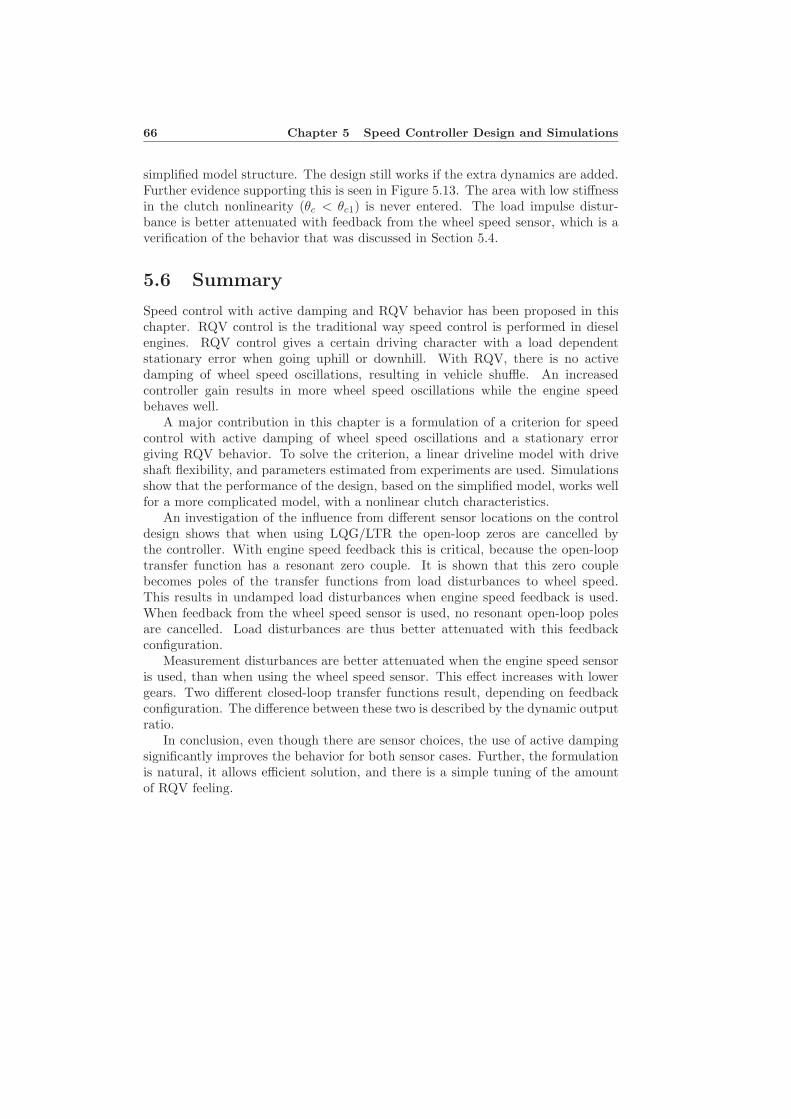
66 Chapter 5 Speed Controller Design and Simulations
simplified model structure. The design still works if the extra dynamics are added.Further evidence supporting this is seen in Figure 5.13. The area with low stiffnessin the clutch nonlinearity (θc < θc1) is never entered. The load impulse distur-bance is better attenuated with feedback from the wheel speed sensor, which is averification of the behavior that was discussed in Section 5.4.
5.6 Summary
Speed control with active damping and RQV behavior has been proposed in thischapter. RQV control is the traditional way speed control is performed in dieselengines. RQV control gives a certain driving character with a load dependentstationary error when going uphill or downhill. With RQV, there is no activedamping of wheel speed oscillations, resulting in vehicle shuffle. An increasedcontroller gain results in more wheel speed oscillations while the engine speedbehaves well.
A major contribution in this chapter is a formulation of a criterion for speedcontrol with active damping of wheel speed oscillations and a stationary errorgiving RQV behavior. To solve the criterion, a linear driveline model with driveshaft flexibility, and parameters estimated from experiments are used. Simulationsshow that the performance of the design, based on the simplified model, works wellfor a more complicated model, with a nonlinear clutch characteristics.
An investigation of the influence from different sensor locations on the controldesign shows that when using LQG/LTR the open-loop zeros are cancelled bythe controller. With engine speed feedback this is critical, because the open-looptransfer function has a resonant zero couple. It is shown that this zero couplebecomes poles of the transfer functions from load disturbances to wheel speed.This results in undamped load disturbances when engine speed feedback is used.When feedback from the wheel speed sensor is used, no resonant open-loop polesare cancelled. Load disturbances are thus better attenuated with this feedbackconfiguration.
Measurement disturbances are better attenuated when the engine speed sensoris used, than when using the wheel speed sensor. This effect increases with lowergears. Two different closed-loop transfer functions result, depending on feedbackconfiguration. The difference between these two is described by the dynamic outputratio.
In conclusion, even though there are sensor choices, the use of active dampingsignificantly improves the behavior for both sensor cases. Further, the formulationis natural, it allows efficient solution, and there is a simple tuning of the amountof RQV feeling.
6Gear-Shift Controller Design and
Simulations
Traditionally a gear shift is performed by disengaging the clutch, engaging neutralgear, shifting to a new gear, and engaging the clutch again. In todays traffic it isdesired to have an automatic gear shifting system, where the complete shift actionis controlled by a microprocessor. If the automatic gear shifting system is to workwith a clutch and a manually shifted transmission, one of the following strategiescan be taken.
• The gear shift is performed with a microprocessor controlling the clutch andthe shift event.
• The gear shift is performed without using the clutch (Orehall 1995). In thiscase the engine is controlled such that the torque in the transmission is zero,whereafter neutral gear is engaged. The engine speed is then controlled to thepropeller shaft speed (scaled with the new conversion ratio). Following that,the new gear is engaged, and then the speed controller controls the drivelineto the speed demanded by the driver.
When using the second approach, neutral gear is engaged when the transmissiontransfers zero torque. It is clear that driveline oscillations is an important perfor-mance limiting factor if they are not damped out. This is because the system hasto wait until satisfactory gear shift conditions are reached, and thus seriously in-creasing the total time needed for a gear shift. One reason this is not acceptableis that, since there is no torque, the vehicle is free rolling which may be seriouswith heavy loads and large road slopes. The observation that the vehicle is freerolling, i.e. changing its velocity, when obtaining gear shift conditions shows thatthe desired control goal is not a stationary point, which has to be handled.
67
68 Chapter 6 Gear-Shift Controller Design and Simulations
This chapter is devoted to study a new idea that the transmission torque canbe estimated and controlled to zero while having active damping. The problemformulation is further discussed in Section 6.1. A model of the transmission isdeveloped and the torque transmitted in the transmission is modeled as a functionof the states and the control signal in Section 6.2. Some first primitive attemptsare then discussed in Section 6.3.
A key result in this chapter is, in light of the simplistic attempts in Section 6.3,the formulation of the gear-shift control criterion in Section 6.4, and its treatmentin Section 6.5. Influence from sensor location and simulations are presented in thesections following.
6.1 Problem Formulation
The gear-shift controller is the controller that drives the transmission torque tozero, while damping oscillations. If a gear shift is commanded when the drivelineis oscillating, the gear-shift controller should still drive the transmission torque tozero.
The control signal is restricted to be in the interval between umin = −300Nm and umax = 2300 Nm. The time it takes for a gear shift should be possibleto optimize. The influence from load and measurement disturbances should beminimized.
6.2 Transmission Torque
The performance output z for the gear-shift controller is the torque transmittedbetween the cog wheels in the transmission. A more detailed study of the trans-mission is depicted in Figure 6.1. Here, the input shaft is connected to bearingswith a viscous friction component bt1. A cog wheel is mounted at the end of theinput shaft which is connected to a cog wheel mounted on the output shaft. Theconversion ratio between these are it, as mentioned in Chapter 2. The output shaftis also connected to bearings with the viscous friction component bt2.
Two equations describe the inputs and outputs of the transmission
Jt1θc = Mt − bt1θc − z (6.1)Jt2θt = itz − bt2θt − Mp (6.2)
6.2.1 Transmission Torque for Model 1
By using (2.1)Jmθm = Mm − Mfr:m − Mc (6.3)
together with (2.12)Mc = Mt, θm = θc (6.4)
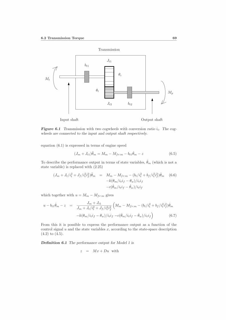
6.2 Transmission Torque 69
Mt
Transmission
θc
θt
bt2
bt1
Jt1
Jt2
Input shaft Output shaft
Mp
Figure 6.1 Transmission with two cogwheels with conversion ratio it. The cog-wheels are connected to the input and output shaft respectively.
equation (6.1) is expressed in terms of engine speed
(Jm + Jt1)θm = Mm − Mfr:m − bt1θm − z (6.5)
To describe the performance output in terms of state variables, θm (which is not astate variable) is replaced with (2.25)
(Jm + Jt/i2t + Jf/i2t i2f )θm = Mm − Mfr:m − (bt/i2t + bf/i2t i
2f )θm (6.6)
−k(θm/itif − θw)/itif
−c(θm/itif − θw)/itif
which together with u = Mm − Mfr:m gives
u − bt1θm − z =Jm + Jt1
Jm + Jt/i2t + Jf/i2t i2f
(Mm − Mfr:m − (bt/i2t + bf/i2t i
2f )θm
−k(θm/itif − θw)/itif −c(θm/itif − θw)/itif
)(6.7)
From this it is possible to express the performance output as a function of thecontrol signal u and the state variables x, according to the state-space description(4.2) to (4.5).
Definition 6.1 The performance output for Model 1 is
z = Mx + Du with
70 Chapter 6 Gear-Shift Controller Design and Simulations
MT =
(Jm+Jt1)kJ1i
Jm+Jt1J1
(b1 + c/i2) − bt1
− (Jm+Jt1)cJ1i
(6.8)
D = 1 − Jm + Jt1
J1
where the labels from (4.5) are used.
The unknown parameters in (6.8) are Jm + Jt1 and bt1. The other parametersare estimated in Chapter 3.
One way of estimating these unknowns would be to decouple Model 1 into twomodels, corresponding to neutral gear. Then a model including the engine, clutch,and the input shaft of the transmission results, in which the performance output zis equal to zero. Trials with neutral gear would then give a possibility to estimatethe unknowns.
In the derivation of Model 1 in Chapter 2 the performance output z is elimi-nated. If z is eliminated in (6.1) and (6.2) and (6.4) is used, the equation for thetransmission is
(Jt1i2t + Jt2)θm = i2t Mc − itMp − (bt1i
2t + bt2)θm (6.9)
By comparing this with the equation describing the transmission in Chapter 2,(2.15)
Jtθm = i2t Mc − btθm − itMp (6.10)
the following equations relating the parameters are obtained
Jt = i2t Jt1 + Jt2 (6.11)bt = i2t bt1 + bt2 (6.12)
For the rest of this chapter the following assumption about the parameters inthe transmission is used.
Assumption 6.1 Jt1 = Jt2 and bt1 = bt2.
Then (6.11) and (6.12) gives
Jt1 =Jt
1 + i2t(6.13)
bt1 =bt
1 + i2t(6.14)
In Chapter 3, the estimated combinations of parameters from Model 1 are
J1 = Jm + Jt/i2t + Jf/i2t i2f (6.15)
b1 = bt/i2t + bf/i2t i2f (6.16)
6.2 Transmission Torque 71
From (6.13) and (6.15) Jm + Jt1 can be derived
Jm + Jt1 = Jm +Jt
1 + i2t= Jm +
i2t1 + i2t
(J1 − Jm − Jf/i2t i2f )
= Jm1
1 + i2t+ J1
i2t1 + i2t
− Jf1
i2f (1 + i2t )(6.17)
A combination of (6.14) and (6.16) gives bt1
bt1 =bt
1 + i2t=
i2t1 + i2t
(b1 − bf/i2t i2f ) (6.18)
For low gears (it large), and since Jf and bf are considerably less than J1 and b1,the following assumptions are used
Jm + Jt1 ≈ J1i2t
1 + i2t(6.19)
bt1 ≈ b1i2t
1 + i2t(6.20)
6.2.2 Transmission Torque for Model 2
The performance output expressed for Model 2 is given by replacing Mt in (6.1)by equation (2.39)
Mc = Mt = kc(θm − θtit) + cc(θm − θtit) (6.21)
Then the performance output is
z = kc(θm − θtit) + cc(θm − θtit) − bt1itθt − Jt1itθt (6.22)
This is expressed in terms of state variables by using (2.45)
(Jt + Jf/i2f )θt = it
(kc(θm − θtit) + cc(θm − θtit)
)(6.23)
−(bt + bf/i2f )θt − 1if
(kd(θt/if − θw) + cd(θt/if − θw)
)
(6.24)
leading to
Definition 6.2 The performance output for Model 2 is
z = Mx with (6.25)
MT =
kc(1 − Jt1i2tJ2
)Jt1itkd
J2if
cc(1 − Jt1i2tJ2
)Jt1i2t
J2(i2t cc + b2 + cd/i2f ) − ccit − bt1it
−Jt1itcd
J2if
72 Chapter 6 Gear-Shift Controller Design and Simulations
with states and labels according to to the state-space description (4.6) to (4.8).
In Chapter 3, the following combinations of parameters from Model 2 are esti-mated.
J2 = Jt + Jf/i2f (6.26)
b2 = bt + bf/i2f (6.27)
From (6.13) , (6.14) , (6.26), and (6.27), Jt1 and bt1 can be derived as
Jt1 =i2t
1 + i2t(J2 − Jf/i2f ) (6.28)
bt1 =i2t
1 + i2t(b2 − bf/i2f ) (6.29)
which are approximated to
Jt1 ≈ i2t1 + i2t
J2 (6.30)
bt1 ≈ i2t1 + i2t
b2 (6.31)
since Jf and bf are considerably less than J1 and b1.
6.2.3 Transmission Torque for Model 3
The performance output for Model 3 is derived in the same way as for Model 2,with the difference that (6.21) is replaced by
Mc = Mt = Mkc(θm − θtit) + cc(θm − θtit) (6.32)
where Mkc is the torque transmitted by the clutch nonlinearity, given by (2.48).Then the performance output is defined as
Definition 6.3 The performance output for Model 3 is
z = (Mkc, θt/if − θw, θm, θt, θw)
1 − Jt1i2tJ2
Jt1itkd
J2if
cc(1 − Jt1i2tJ2
)Jt1i2t
J2(i2t cc + b2 + cd/i2f ) − ccit − bt1it
−Jt1itcd
J2if
(6.33)
The parameters not estimated in the definition above are approximated in thesame way as for the performance output for Model 2.
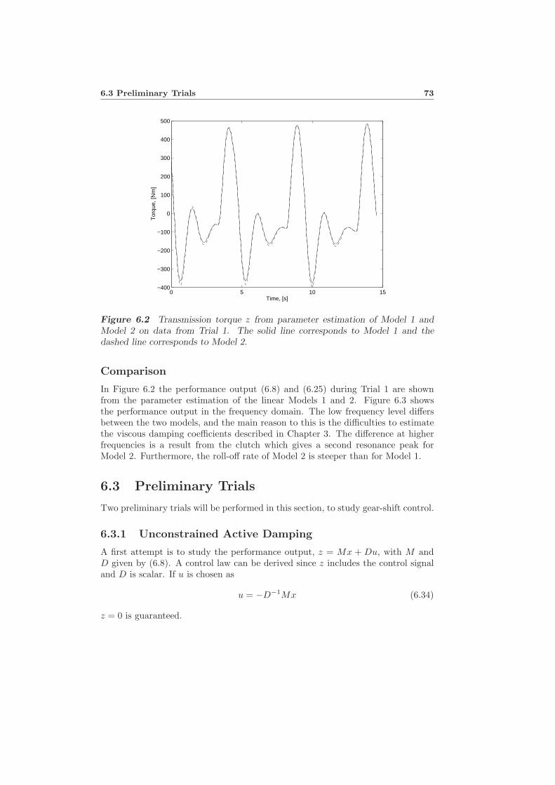
6.3 Preliminary Trials 73
0 5 10 15−400
−300
−200
−100
0
100
200
300
400
500
Time, [s]
Tor
que,
[Nm
]
Figure 6.2 Transmission torque z from parameter estimation of Model 1 andModel 2 on data from Trial 1. The solid line corresponds to Model 1 and thedashed line corresponds to Model 2.
Comparison
In Figure 6.2 the performance output (6.8) and (6.25) during Trial 1 are shownfrom the parameter estimation of the linear Models 1 and 2. Figure 6.3 showsthe performance output in the frequency domain. The low frequency level differsbetween the two models, and the main reason to this is the difficulties to estimatethe viscous damping coefficients described in Chapter 3. The difference at higherfrequencies is a result from the clutch which gives a second resonance peak forModel 2. Furthermore, the roll-off rate of Model 2 is steeper than for Model 1.
6.3 Preliminary Trials
Two preliminary trials will be performed in this section, to study gear-shift control.
6.3.1 Unconstrained Active Damping
A first attempt is to study the performance output, z = Mx + Du, with M andD given by (6.8). A control law can be derived since z includes the control signaland D is scalar. If u is chosen as
u = −D−1Mx (6.34)
z = 0 is guaranteed.
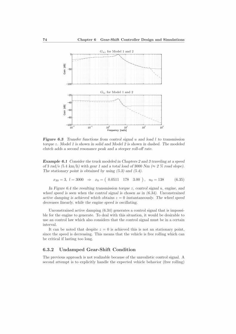
74 Chapter 6 Gear-Shift Controller Design and Simulations
−100
−50
0
Gai
n [d
B]
10−2
10−1
100
101
102
103
−100
−80
−60
−40
−20
Frequency [rad/s]
Gai
n [d
B]
Guz for Model 1 and 2
Glz for Model 1 and 2
Figure 6.3 Transfer functions from control signal u and load l to transmissiontorque z. Model 1 is shown in solid and Model 2 is shown in dashed. The modeledclutch adds a second resonance peak and a steeper roll-off rate.
Example 6.1 Consider the truck modeled in Chapters 2 and 3 traveling at a speedof 3 rad/s (5.4 km/h) with gear 1 and a total load of 3000 Nm (≈ 2 % road slope).The stationary point is obtained by using (5.3) and (5.4).
x30 = 3, l = 3000 ⇒ x0 =(
0.0511 178 3.00), u0 = 138 (6.35)
In Figure 6.4 the resulting transmission torque z, control signal u, engine, andwheel speed is seen when the control signal is chosen as in (6.34). Unconstrainedactive damping is achieved which obtains z = 0 instantaneously. The wheel speeddecreases linearly, while the engine speed is oscillating.
Unconstrained active damping (6.34) generates a control signal that is impossi-ble for the engine to generate. To deal with this situation, it would be desirable touse an control law which also considers that the control signal must be in a certaininterval.
It can be noted that despite z = 0 is achieved this is not an stationary point,since the speed is decreasing. This means that the vehicle is free rolling which canbe critical if lasting too long.
6.3.2 Undamped Gear-Shift Condition
The previous approach is not realizable because of the unrealistic control signal. Asecond attempt is to explicitly handle the expected vehicle behavior (free rolling)
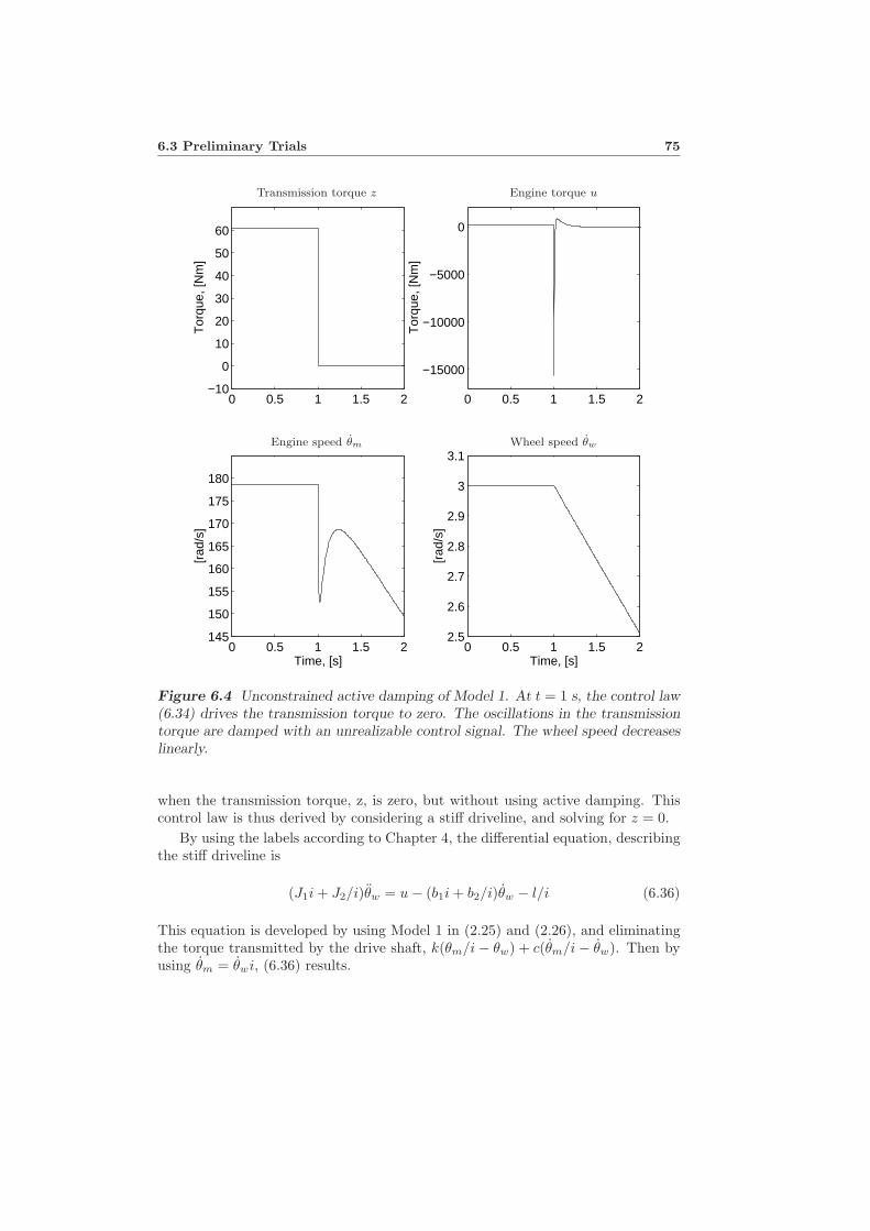
6.3 Preliminary Trials 75
0 0.5 1 1.5 2−10
0
10
20
30
40
50
60
Tor
que,
[Nm
]
0 0.5 1 1.5 2
−15000
−10000
−5000
0
Tor
que,
[Nm
]
0 0.5 1 1.5 2145
150
155
160
165
170
175
180
[rad
/s]
Time, [s]0 0.5 1 1.5 2
2.5
2.6
2.7
2.8
2.9
3
3.1
Time, [s]
[rad
/s]
Transmission torque z Engine torque u
Engine speed θm Wheel speed θw
Figure 6.4 Unconstrained active damping of Model 1. At t = 1 s, the control law(6.34) drives the transmission torque to zero. The oscillations in the transmissiontorque are damped with an unrealizable control signal. The wheel speed decreaseslinearly.
when the transmission torque, z, is zero, but without using active damping. Thiscontrol law is thus derived by considering a stiff driveline, and solving for z = 0.
By using the labels according to Chapter 4, the differential equation, describingthe stiff driveline is
(J1i + J2/i)θw = u − (b1i + b2/i)θw − l/i (6.36)
This equation is developed by using Model 1 in (2.25) and (2.26), and eliminatingthe torque transmitted by the drive shaft, k(θm/i − θw) + c(θm/i − θw). Then byusing θm = θwi, (6.36) results.
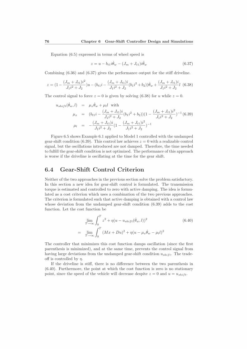
76 Chapter 6 Gear-Shift Controller Design and Simulations
Equation (6.5) expressed in terms of wheel speed is
z = u − bt1iθw − (Jm + Jt1)iθw (6.37)
Combining (6.36) and (6.37) gives the performance output for the stiff driveline.
z = (1− (Jm + Jt1)i2
J1i2 + J2)u− (bt1i− (Jm + Jt1)i
J1i2 + J2(b1i
2 + b2))θw +(Jm + Jt1)iJ1i2 + J2
l (6.38)
The control signal to force z = 0 is given by solving (6.38) for u while z = 0.
ushift(θw, l) = µxθw + µll with
µx = (bt1i − (Jm + Jt1)iJ1i2 + J2
(b1i2 + b2))(1 − (Jm + Jt1)i2
J1i2 + J2)−1 (6.39)
µl = − (Jm + Jt1)iJ1i2 + J2
(1 − (Jm + Jt1)i2
J1i2 + J2)−1
Figure 6.5 shows Example 6.1 applied to Model 1 controlled with the undampedgear-shift condition (6.39). This control law achieves z = 0 with a realizable controlsignal, but the oscillations introduced are not damped. Therefore, the time neededto fulfill the gear-shift condition is not optimized. The performance of this approachis worse if the driveline is oscillating at the time for the gear shift.
6.4 Gear-Shift Control Criterion
Neither of the two approaches in the previous section solve the problem satisfactory.In this section a new idea for gear-shift control is formulated. The transmissiontorque is estimated and controlled to zero with active damping. The idea is formu-lated as a cost criterion which uses a combination of the two previous approaches.The criterion is formulated such that active damping is obtained with a control lawwhose deviation from the undamped gear-shift condition (6.39) adds to the costfunction. Let the cost function be
limT→∞
∫ T
0
z2 + η(u − ushift(θw, l))2 (6.40)
= limT→∞
∫ T
0
(Mx + Du)2 + η(u − µxθw − µll)2
The controller that minimizes this cost function damps oscillation (since the firstparenthesis is minimized), and at the same time, prevents the control signal fromhaving large deviations from the undamped gear-shift condition ushift. The trade-off is controlled by η.
If the driveline is stiff, there is no difference between the two parenthesis in(6.40). Furthermore, the point at which the cost function is zero is no stationarypoint, since the speed of the vehicle will decrease despite z = 0 and u = ushift.
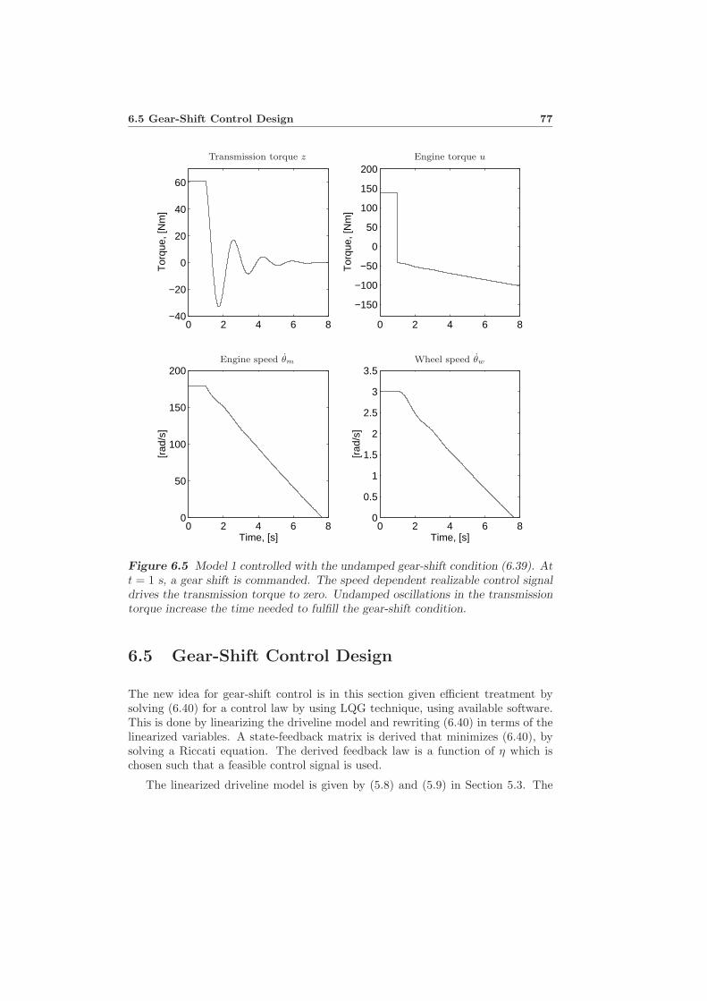
6.5 Gear-Shift Control Design 77
0 2 4 6 8−40
−20
0
20
40
60
Tor
que,
[Nm
]
0 2 4 6 8
−150
−100
−50
0
50
100
150
200
Tor
que,
[Nm
]
0 2 4 6 80
50
100
150
200
Time, [s]
[rad
/s]
0 2 4 6 80
0.5
1
1.5
2
2.5
3
3.5
Time, [s]
[rad
/s]
Transmission torque z Engine torque u
Engine speed θm Wheel speed θw
Figure 6.5 Model 1 controlled with the undamped gear-shift condition (6.39). Att = 1 s, a gear shift is commanded. The speed dependent realizable control signaldrives the transmission torque to zero. Undamped oscillations in the transmissiontorque increase the time needed to fulfill the gear-shift condition.
6.5 Gear-Shift Control Design
The new idea for gear-shift control is in this section given efficient treatment bysolving (6.40) for a control law by using LQG technique, using available software.This is done by linearizing the driveline model and rewriting (6.40) in terms of thelinearized variables. A state-feedback matrix is derived that minimizes (6.40), bysolving a Riccati equation. The derived feedback law is a function of η which ischosen such that a feasible control signal is used.
The linearized driveline model is given by (5.8) and (5.9) in Section 5.3. The
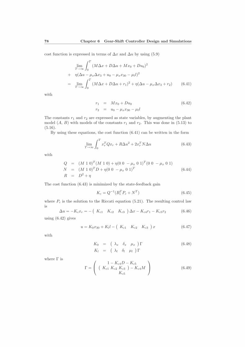
78 Chapter 6 Gear-Shift Controller Design and Simulations
cost function is expressed in terms of ∆x and ∆u by using (5.9)
limT→∞
∫ T
0
(M∆x + D∆u + Mx0 + Du0)2
+ η(∆u − µx∆x3 + u0 − µxx30 − µll)2
= limT→∞
∫ T
0
(M∆x + D∆u + r1)2 + η(∆u − µx∆x3 + r2) (6.41)
with
r1 = Mx0 + Du0 (6.42)r2 = u0 − µxx30 − µll
The constants r1 and r2 are expressed as state variables, by augmenting the plantmodel (A, B) with models of the constants r1 and r2. This was done in (5.13) to(5.16).
By using these equations, the cost function (6.41) can be written in the form
limT→∞
∫ T
0
xTr Qxr + R∆u2 + 2xT
r N∆u (6.43)
with
Q = (M 1 0)T (M 1 0) + η(0 0 − µx 0 1)T (0 0 − µx 0 1)N = (M 1 0)T D + η(0 0 − µx 0 1)T (6.44)R = D2 + η
The cost function (6.43) is minimized by the state-feedback gain
Kc = Q−1(BTr Pc + NT ) (6.45)
where Pc is the solution to the Riccati equation (5.21). The resulting control lawis
∆u = −Kcxr = − (Kc1 Kc2 Kc3
)∆x − Kc4r1 − Kc5r2 (6.46)
using (6.42) gives
u = K0x30 + Kll −(
Kc1 Kc2 Kc3
)x (6.47)
with
K0 =(
λx δx µx
)Γ (6.48)
Kl =(
λl δl µl
)Γ
where Γ is
Γ =
1 − Kc4D − Kc5(
Kc1 Kc2 Kc3
) − Kc4MKc5
(6.49)
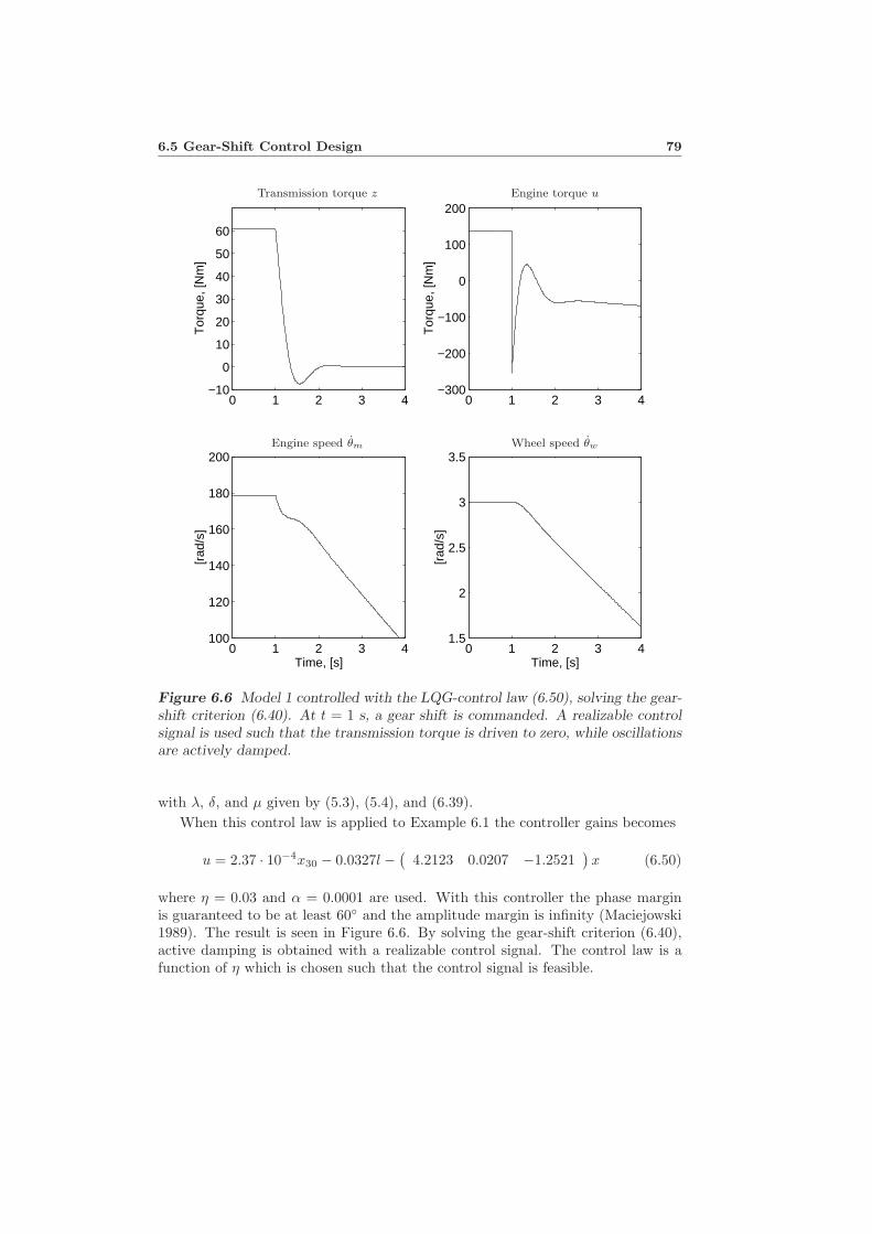
6.5 Gear-Shift Control Design 79
0 1 2 3 4−10
0
10
20
30
40
50
60
Tor
que,
[Nm
]
0 1 2 3 4−300
−200
−100
0
100
200
Tor
que,
[Nm
]
0 1 2 3 4100
120
140
160
180
200
Time, [s]
[rad
/s]
0 1 2 3 41.5
2
2.5
3
3.5
Time, [s]
[rad
/s]
Transmission torque z Engine torque u
Engine speed θm Wheel speed θw
Figure 6.6 Model 1 controlled with the LQG-control law (6.50), solving the gear-shift criterion (6.40). At t = 1 s, a gear shift is commanded. A realizable controlsignal is used such that the transmission torque is driven to zero, while oscillationsare actively damped.
with λ, δ, and µ given by (5.3), (5.4), and (6.39).When this control law is applied to Example 6.1 the controller gains becomes
u = 2.37 · 10−4x30 − 0.0327l − (4.2123 0.0207 −1.2521
)x (6.50)
where η = 0.03 and α = 0.0001 are used. With this controller the phase marginis guaranteed to be at least 60◦ and the amplitude margin is infinity (Maciejowski1989). The result is seen in Figure 6.6. By solving the gear-shift criterion (6.40),active damping is obtained with a realizable control signal. The control law is afunction of η which is chosen such that the control signal is feasible.
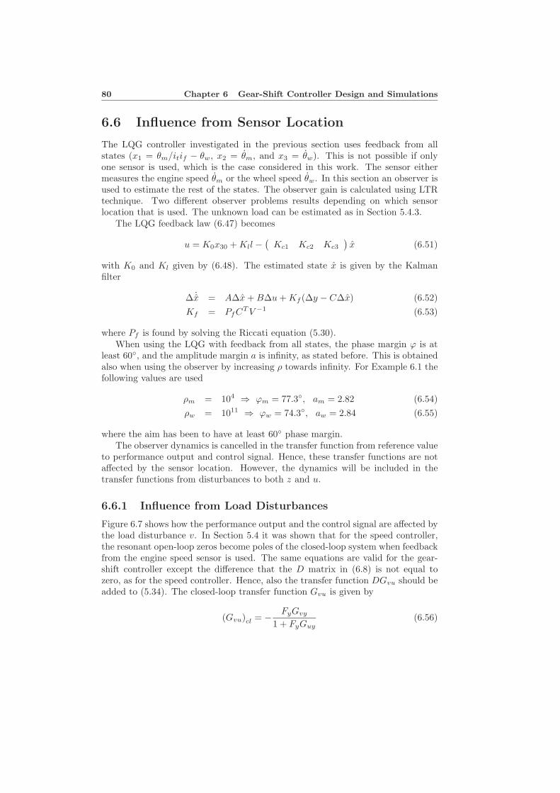
80 Chapter 6 Gear-Shift Controller Design and Simulations
6.6 Influence from Sensor Location
The LQG controller investigated in the previous section uses feedback from allstates (x1 = θm/itif − θw, x2 = θm, and x3 = θw). This is not possible if onlyone sensor is used, which is the case considered in this work. The sensor eithermeasures the engine speed θm or the wheel speed θw. In this section an observer isused to estimate the rest of the states. The observer gain is calculated using LTRtechnique. Two different observer problems results depending on which sensorlocation that is used. The unknown load can be estimated as in Section 5.4.3.
The LQG feedback law (6.47) becomes
u = K0x30 + Kll −(
Kc1 Kc2 Kc3
)x (6.51)
with K0 and Kl given by (6.48). The estimated state x is given by the Kalmanfilter
∆ ˙x = A∆x + B∆u + Kf (∆y − C∆x) (6.52)Kf = PfCT V −1 (6.53)
where Pf is found by solving the Riccati equation (5.30).When using the LQG with feedback from all states, the phase margin ϕ is at
least 60◦, and the amplitude margin a is infinity, as stated before. This is obtainedalso when using the observer by increasing ρ towards infinity. For Example 6.1 thefollowing values are used
ρm = 104 ⇒ ϕm = 77.3◦, am = 2.82 (6.54)ρw = 1011 ⇒ ϕw = 74.3◦, aw = 2.84 (6.55)
where the aim has been to have at least 60◦ phase margin.The observer dynamics is cancelled in the transfer function from reference value
to performance output and control signal. Hence, these transfer functions are notaffected by the sensor location. However, the dynamics will be included in thetransfer functions from disturbances to both z and u.
6.6.1 Influence from Load Disturbances
Figure 6.7 shows how the performance output and the control signal are affected bythe load disturbance v. In Section 5.4 it was shown that for the speed controller,the resonant open-loop zeros become poles of the closed-loop system when feedbackfrom the engine speed sensor is used. The same equations are valid for the gear-shift controller except the difference that the D matrix in (6.8) is not equal tozero, as for the speed controller. Hence, also the transfer function DGvu should beadded to (5.34). The closed-loop transfer function Gvu is given by
(Gvu)cl = − FyGvy
1 + FyGuy(6.56)
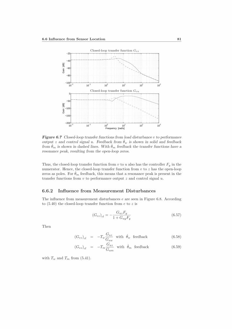
6.6 Influence from Sensor Location 81
10−2
10−1
100
101
102
103
−100
−80
−60
−40
−20
Gai
n [d
B]
10−2
10−1
100
101
102
103
−200
−150
−100
−50
0
Frequency [rad/s]
Gai
n [d
B]
Closed-loop transfer function Gvz
Closed-loop transfer function Gvu
Figure 6.7 Closed-loop transfer functions from load disturbance v to performanceoutput z and control signal u. Feedback from θw is shown in solid and feedbackfrom θm is shown in dashed lines. With θm feedback the transfer functions have aresonance peak, resulting from the open-loop zeros.
Thus, the closed-loop transfer function from v to u also has the controller Fy in thenumerator. Hence, the closed-loop transfer function from v to z has the open-loopzeros as poles. For θm feedback, this means that a resonance peak is present in thetransfer functions from v to performance output z and control signal u.
6.6.2 Influence from Measurement Disturbances
The influence from measurement disturbances e are seen in Figure 6.8. Accordingto (5.40) the closed-loop transfer function from e to z is
(Gez)cl = − GuzFy
1 + GuyFy(6.57)
Then
(Gez)cl = −TwGuz
Guwwith θw feedback (6.58)
(Gez)cl = −TmGuz
Gumwith θm feedback (6.59)
with Tw and Tm from (5.41).
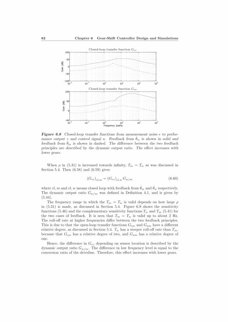
82 Chapter 6 Gear-Shift Controller Design and Simulations
10−2
10−1
100
101
102
103
−100
−50
0
50
100
Gai
n [d
B]
10−2
10−1
100
101
102
103
−50
0
50
100
Frequency [rad/s]
Gai
n [d
B]
Closed-loop transfer function Gez
Closed-loop transfer function Geu
Figure 6.8 Closed-loop transfer functions from measurement noise e to perfor-mance output z and control signal u. Feedback from θw is shown in solid andfeedback from θm is shown in dashed. The difference between the two feedbackprinciples are described by the dynamic output ratio. The effect increases withlower gears.
When ρ in (5.31) is increased towards infinity, Tm = Tw as was discussed inSection 5.4. Then (6.58) and (6.59) gives
(Gez)cl,m = (Gez)cl,w Gw/m (6.60)
where cl,m and cl, w means closed loop with feedback from θm and θw respectively.The dynamic output ratio Gw/m was defined in Definition 4.1, and is given by(5.44).
The frequency range in which the Tm = Tw is valid depends on how large ρin (5.31) is made, as discussed in Section 5.4. Figure 6.9 shows the sensitivityfunctions (5.46) and the complementary sensitivity functions Tw and Tm (5.41) forthe two cases of feedback. It is seen that Tm = Tw is valid up to about 2 Hz.The roll-off rate at higher frequencies differ between the two feedback principles.This is due to that the open-loop transfer functions Guw and Gum have a differentrelative degree, as discussed in Section 5.4. Tw has a steeper roll-off rate than Tm,because that Guw has a relative degree of two, and Gum has a relative degree ofone.
Hence, the difference in Gez depending on sensor location is described by thedynamic output ratio Gw/m. The difference in low frequency level is equal to theconversion ratio of the driveline. Therefore, this effect increases with lower gears.
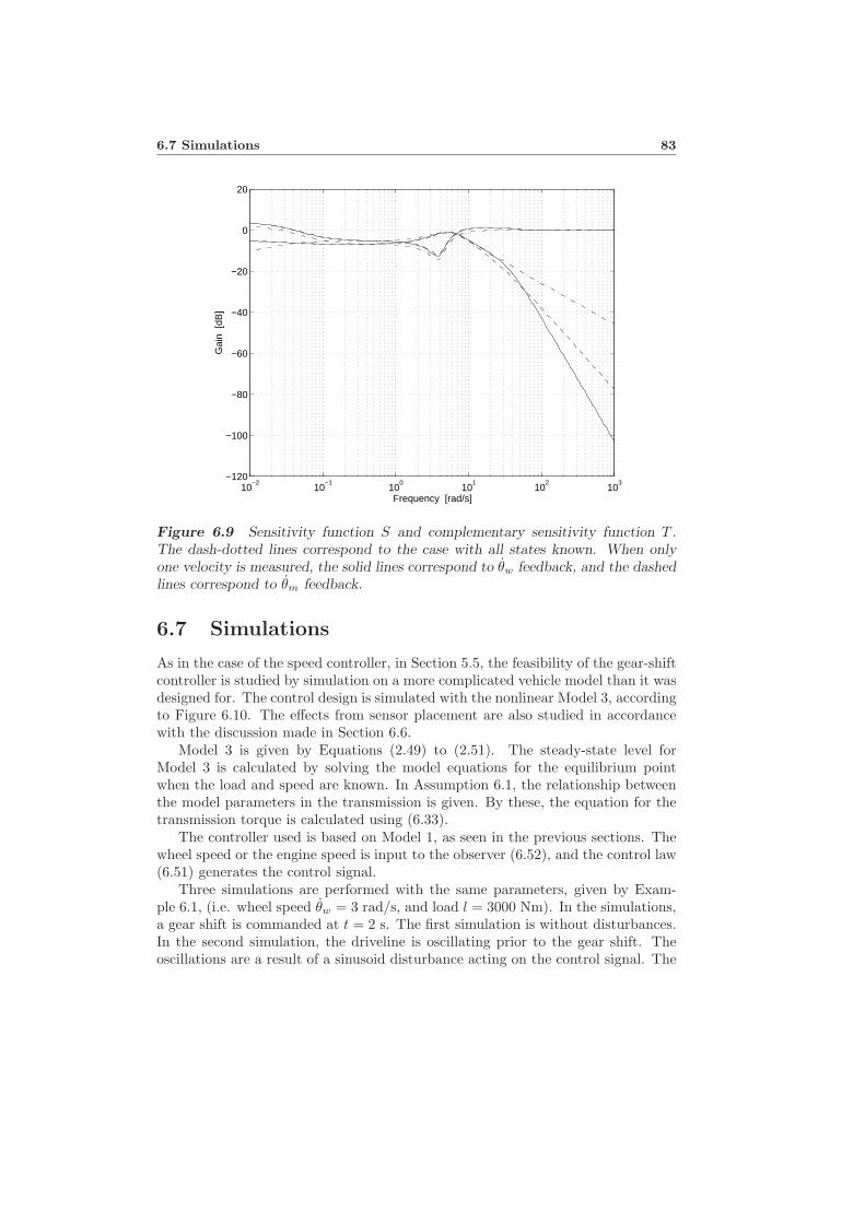
6.7 Simulations 83
10−2
10−1
100
101
102
103
−120
−100
−80
−60
−40
−20
0
20
Frequency [rad/s]
Gai
n [d
B]
Figure 6.9 Sensitivity function S and complementary sensitivity function T .The dash-dotted lines correspond to the case with all states known. When onlyone velocity is measured, the solid lines correspond to θw feedback, and the dashedlines correspond to θm feedback.
6.7 Simulations
As in the case of the speed controller, in Section 5.5, the feasibility of the gear-shiftcontroller is studied by simulation on a more complicated vehicle model than it wasdesigned for. The control design is simulated with the nonlinear Model 3, accordingto Figure 6.10. The effects from sensor placement are also studied in accordancewith the discussion made in Section 6.6.
Model 3 is given by Equations (2.49) to (2.51). The steady-state level forModel 3 is calculated by solving the model equations for the equilibrium pointwhen the load and speed are known. In Assumption 6.1, the relationship betweenthe model parameters in the transmission is given. By these, the equation for thetransmission torque is calculated using (6.33).
The controller used is based on Model 1, as seen in the previous sections. Thewheel speed or the engine speed is input to the observer (6.52), and the control law(6.51) generates the control signal.
Three simulations are performed with the same parameters, given by Exam-ple 6.1, (i.e. wheel speed θw = 3 rad/s, and load l = 3000 Nm). In the simulations,a gear shift is commanded at t = 2 s. The first simulation is without disturbances.In the second simulation, the driveline is oscillating prior to the gear shift. Theoscillations are a result of a sinusoid disturbance acting on the control signal. The
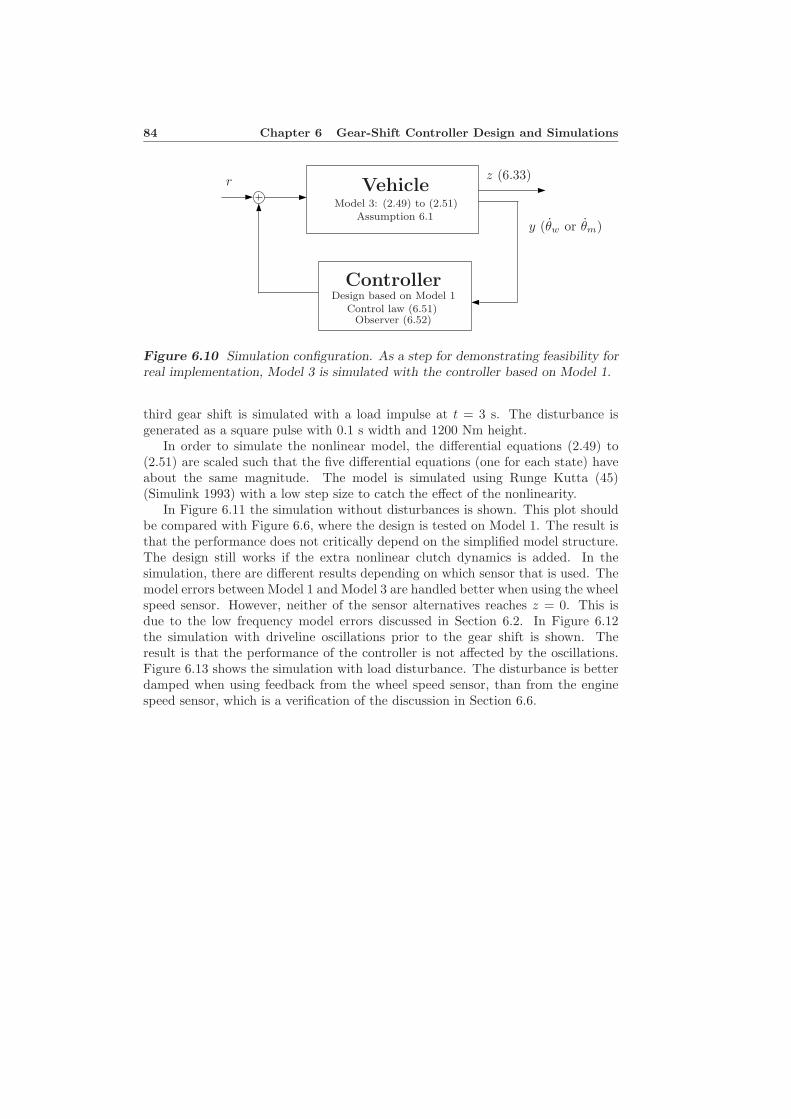
84 Chapter 6 Gear-Shift Controller Design and Simulations
ControllerDesign based on Model 1
Control law (6.51)Observer (6.52)
z (6.33)
y (θw or θm)
r VehicleModel 3: (2.49) to (2.51)
Assumption 6.1
Figure 6.10 Simulation configuration. As a step for demonstrating feasibility forreal implementation, Model 3 is simulated with the controller based on Model 1.
third gear shift is simulated with a load impulse at t = 3 s. The disturbance isgenerated as a square pulse with 0.1 s width and 1200 Nm height.
In order to simulate the nonlinear model, the differential equations (2.49) to(2.51) are scaled such that the five differential equations (one for each state) haveabout the same magnitude. The model is simulated using Runge Kutta (45)(Simulink 1993) with a low step size to catch the effect of the nonlinearity.
In Figure 6.11 the simulation without disturbances is shown. This plot shouldbe compared with Figure 6.6, where the design is tested on Model 1. The result isthat the performance does not critically depend on the simplified model structure.The design still works if the extra nonlinear clutch dynamics is added. In thesimulation, there are different results depending on which sensor that is used. Themodel errors between Model 1 and Model 3 are handled better when using the wheelspeed sensor. However, neither of the sensor alternatives reaches z = 0. This isdue to the low frequency model errors discussed in Section 6.2. In Figure 6.12the simulation with driveline oscillations prior to the gear shift is shown. Theresult is that the performance of the controller is not affected by the oscillations.Figure 6.13 shows the simulation with load disturbance. The disturbance is betterdamped when using feedback from the wheel speed sensor, than from the enginespeed sensor, which is a verification of the discussion in Section 6.6.
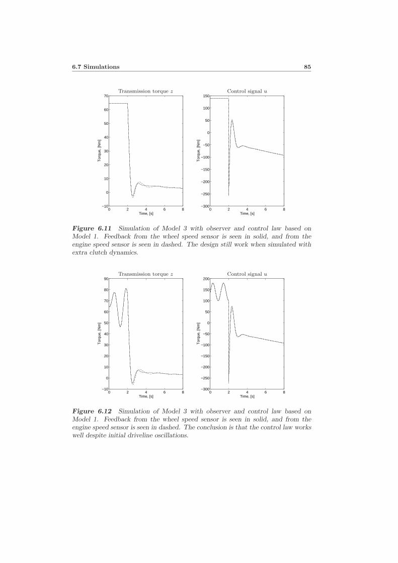
6.7 Simulations 85
0 2 4 6 8−10
0
10
20
30
40
50
60
70
Time, [s]
Tor
que,
[Nm
]
0 2 4 6 8−300
−250
−200
−150
−100
−50
0
50
100
150
Time, [s]
Tor
que,
[Nm
]
Transmission torque z Control signal u
Figure 6.11 Simulation of Model 3 with observer and control law based onModel 1. Feedback from the wheel speed sensor is seen in solid, and from theengine speed sensor is seen in dashed. The design still work when simulated withextra clutch dynamics.
0 2 4 6 8−10
0
10
20
30
40
50
60
70
80
90
Time, [s]
Tor
que,
[Nm
]
0 2 4 6 8−300
−250
−200
−150
−100
−50
0
50
100
150
200
Time, [s]
Tor
que,
[Nm
]
Transmission torque z Control signal u
Figure 6.12 Simulation of Model 3 with observer and control law based onModel 1. Feedback from the wheel speed sensor is seen in solid, and from theengine speed sensor is seen in dashed. The conclusion is that the control law workswell despite initial driveline oscillations.
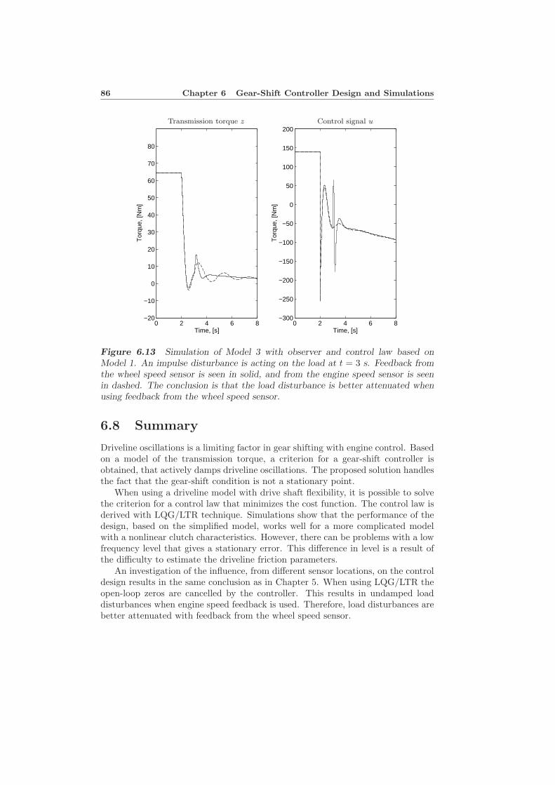
86 Chapter 6 Gear-Shift Controller Design and Simulations
0 2 4 6 8−20
−10
0
10
20
30
40
50
60
70
80
Time, [s]
Tor
que,
[Nm
]
0 2 4 6 8−300
−250
−200
−150
−100
−50
0
50
100
150
200
Time, [s]
Tor
que,
[Nm
]
Transmission torque z Control signal u
Figure 6.13 Simulation of Model 3 with observer and control law based onModel 1. An impulse disturbance is acting on the load at t = 3 s. Feedback fromthe wheel speed sensor is seen in solid, and from the engine speed sensor is seenin dashed. The conclusion is that the load disturbance is better attenuated whenusing feedback from the wheel speed sensor.
6.8 Summary
Driveline oscillations is a limiting factor in gear shifting with engine control. Basedon a model of the transmission torque, a criterion for a gear-shift controller isobtained, that actively damps driveline oscillations. The proposed solution handlesthe fact that the gear-shift condition is not a stationary point.
When using a driveline model with drive shaft flexibility, it is possible to solvethe criterion for a control law that minimizes the cost function. The control law isderived with LQG/LTR technique. Simulations show that the performance of thedesign, based on the simplified model, works well for a more complicated modelwith a nonlinear clutch characteristics. However, there can be problems with a lowfrequency level that gives a stationary error. This difference in level is a result ofthe difficulty to estimate the driveline friction parameters.
An investigation of the influence, from different sensor locations, on the controldesign results in the same conclusion as in Chapter 5. When using LQG/LTR theopen-loop zeros are cancelled by the controller. This results in undamped loaddisturbances when engine speed feedback is used. Therefore, load disturbances arebetter attenuated with feedback from the wheel speed sensor.
6.8 Summary 87
Measurement disturbances are better attenuated when the engine speed sensoris used, than when using the wheel speed sensor. This effect increases with lowergears. Two different closed-loop transfer functions result, depending on feedbackconfiguration. The difference between these two is described by the dynamic outputratio.
In conclusion, actively damped transmission-torque control works well also inthe case of existing initial oscillations. Furthermore, disturbances occuring duringthe control action are actively damped, and thus reducing the time needed for agear shift.

88 Chapter 6 Gear-Shift Controller Design and Simulations
7Conclusions
The driveline is a fundamental component in a vehicle, and there is currentlya strong trend in improving performance by adding functionalities in drivelinemanagement systems.
The major contribution of this thesis is a novel gear shifting strategy basedon modeling of the transmission torque, and design of a criterion for a controllerthat drives this torque to zero. This controller is to be used with a new automaticgear shifting system, utilizing engine controlled gear shifting without using theclutch. The proposed solution offers a possibility to optimize the time needed fora gear shift, which is important since the vehicle is free rolling when in gear-shiftcondition. Furthermore, neutral gear can successfully be engaged also when facingcritical load disturbances and initial driveline oscillations.
A second important contribution is the extension of the traditionally used RQVcontroller. A criterion for a controller that actively damps wheel speed oscillationswith a stationary error characteristic for the RQV controller, is obtained. Withthis controller the performance and driveability is improved since vehicle shuffle isreduced. Furthermore, the formulation is natural, it allows efficient solution, andthere is a simple tuning of the amount of RQV feeling.
A basis for these results is the modeling conclusions drawn from experimentsand modeling using a heavy truck. A key contribution is the observation thata linear model with stiff clutch and drive shaft flexibility is able to explain themeasured engine speed and wheel speed. Extra clutch dynamics is not able toexplain more of the experiments for low frequencies. Therefore, the linear modelis concluded to be a basis for control design, which is verified by simulations on amodel with a nonlinear clutch characteristics.
89
90 Chapter 7 Conclusions
Another important observation from the experiments is the explanation of thedifference between the measured engine speed and transmission speed. The majorpart of the difference is explained by a simple sensor model. Parameter estimationof a nonlinear model shows that the deviations still left occur when the clutchtransfers zero torque.
A common architectural issue in driveline control is the issue of sensor location.Different sensors give the same open-loop poles, but different zeros. An investiga-tion of the influence from different sensor locations on the control design shows thatwhen using LQG/LTR, load disturbances are better damped with feedback fromthe wheel speed, due to well damped open-loop zeros. Measurement disturbancesare better attenuated when the engine speed sensor is used, than when using thewheel speed sensor. The difference is explained by the dynamic output ratio, andincreases with lower gears.
There are thus issues to be considered in sensor choice, but the overall conclusionis that the proposed strategies improve performance and driveability in both speedcontrol and gear-shift control.
Bibliography
Bjornberg, A., M. Pettersson, and L. Nielsen (1996). Nonlinear driveline oscilla-tions at low clutch torques in heavy trucks. To be presented at Reglermotet ’96 inLulea, Sweden.
Bosch (1993). Automotive Handbook. Stuttgart, Germany: Robert Bosch GmbH.
Gillespie, T. D. (1992). Fundamentals of Vehicle Dynamics. SAE International.
Henriksson, T., M. Pettersson, and F. Gustafsson (1993). An investigation of thelongitudinal dynamics of a car, especially air drag and rolling resistance. Tech-nical Report LiTH-ISY-R-1506, Department of Electrical Engineering, LinkopingUniversity.
Kubrusly, C. and H. Malebranche (1985). Sensors and controllers location indistributed systems - a survey. Automatica 21, 117–128.
Liversidge, J. H. (1952). Backlash and Resilience within Closed Loop of AutomaticControl Systems. Academic Press.
Ljung, L. (1988). Control Theory 1984-1986. Automatica 24, 573–583.
Ljung, L. (1995). System Identification Toolbox. User’s Guide. MathWorks, Inc.
Maciejowski, J. M. (1989). Multivariable Feedback Design. Addison-Wesley.
Meriam, J. L. and L. G. Kraige (1987). Dynamics, Volume 2 of EngineeringMechanics. John Wiley & Sons.
91
92 Bibliography
Mo, C. Y., A. J. Beaumount, and N. N. Powell (1996). Active control of drive-ability. SAE Paper 960046.
Nwagboso, C. O. (1993). Automotive Sensory Systems. Chapman & Hall.
Orehall, L. (1995). Scania opticruise: Mechanical gearchanging with engine con-trol. Truck and Commercial Vehicle International ’95.
Pettersson, M. and L. Nielsen (1995). Sensor placement for driveline control.Preprint of the IFAC-Workshop on Advances in Automotive Control, Ascona,Switzerland .
Simulink (1993). User’s guide. MathWorks, Inc.
Spong, M. W. and M. Vidyasagar (1989). Robot Dynamics and Control. JohnWiley & Sons.
Suzuki, K. and Y. Tozawa (1992). Influence of powertrain torsional rigidity onNVH of 6x4 trucks. SAE Paper 922482.
Notations
Variables
r Radius, reference signalu Control signalz Performance outputx State vectory Sensor outputv State disturbance, velocitye Measurement disturbancen Input disturbancel Loadθ Angleα Road slope
Symbols
J Mass moment of inertiai Conversion ratiok Torsional stiffness
93
94 Notations
c Torsional dampingb Viscous friction componentm Vehicle masscr1, cr2 Coefficients of rolling resistancecw Air drag coefficientρa Air densityAa Vehicle cross section areaFa Air resistance forceFr Rolling resistance forceM Torque, performance output state matrixA State-space matrixB Input state matrixC Output state matrixH Load state matrixD Performance output control signal matrixG Transfer functionGw/m Dynamic output ratioS Sensitivity functionT Complementary sensitivity functionKc State-feedback matrixKf Observer gainϕ Phase margina Amplitude margin
Subscripts
m Enginec Clutcht Tranmissionp Propeller shaftf Final drived Drive shaftsw Wheelfr Friction0 Stationary valuet1 Transmission inputt2 Transmission output


![ADAPTIVE CRUISE CONTROL OF A SIMSCAPE DRIVELINE …jestec.taylors.edu.my/Vol 16 issue 1 February 2021/16_1_47.pdflongitudinal vehicle dynamics using Simscape Driveline library [36]](https://img.pdfslide.net/doc/110x75/612eb33c1ecc51586942faa7/adaptive-cruise-control-of-a-simscape-driveline-16-issue-1-february-202116147pdf.jpg)