Embed Size (px)
Citation preview
Driving resistance analysis of long haulage
trucks at Volvo
-Test methods evaluation
Master’s Thesis in the Master’s programme Automotive engineering
HENRIK STENVALL
Department of Applied mechanics
Division of Vehicle engineering & autonomous systems
CHALMERS UNIVERSITY OF TECHNOLOGY
Göteborg, Sweden 2010
Master’s Thesis 2010:18

MASTER’S THESIS 2010:18
Driving resistance analysis of long haulage trucks at Volvo
-Test methods evaluation
Master’s Thesis in the Master’s programme Automotive engineering
HENRIK STENVALL
Department of Applied Mechanics
Division of Vehicle engineering & autonomous systems
CHALMERS UNIVERSITY OF TECHNOLOGY
Göteborg, Sweden 2010
Driving resistance analysis of long haulage trucks at Volvo
-Test methods evaluation
Master’s Thesis in the Master’s programme Automotive engineering
HENRIK STENVALL
© HENRIK STENVALL, 2010
Master’s Thesis 2010:18
ISSN 1652-8557
Department of Applied Mechanics
Division of Vehicle engineering & autonomous systems
Chalmers University of Technology
SE-412 96 Göteborg
Sweden
Telephone: + 46 (0)31-772 1000
Cover:
Volvo FH with T052 trailer equipped with 5th
wheel for coast down test. This vehicle
is the reference vehicle, driven at autumn 2009, for coast down results see Figure 24.
Chalmers repro service
Göteborg, Sweden 2010
I
Driving resistance analysis of long haulage trucks at Volvo
-Test methods evaluation
Master’s Thesis in the Master’s programme Automotive engineering
HENRIK STENVALL
Department of Applied Mechanics
Division of Vehicle engineering & autonomous systems
Chalmers University of Technology
ABSTRACT
To further improve fuel consumption of future trucks and to be able to measure the
gains obtained from new inventions, accurate test methods have to be defined. The
three main tests currently used at Volvo are: road testing, chassis dynamometer and
computer simulations. In this project the three fuel consumption test methods are
evaluated with the Volvo FH and its main rivals to get an indication of the results
reliability. If the test gives different fuel consumptions but has similar percentage
differences between the trucks a fixed relation between test methods is obtained.
The chassis dynamometer’s road load is based on the measured force at the vehicle
for every vehicle speed. To find this relation a coast down test for each truck is
performed; the test is based on continuous logging of vehicle speed and time while
driving the equipage at neutral gear from 85-16 km/h. The tests were done in February
and consequently weather influenced the results, with wet tracks, winds and low
temperatures.
The road tests were carried out in April with less restrictive environment, but also
using bedded tires and different trailers. The resulting fuel consumption at the Lv-Bo-
Lv (Landvetter-Borås-Landvetter) duty cycle for each truck were without exception
lower for the road tests compared to the chassis dynamometer results. The percentage
difference between the tests were not constant for the different trucks but rather close
to the difference in-between trucks attained from the coast downs at full speed, which
reflects the Lv-Bo-Lv duty cycle well, (except for the road inclinations). This proves
that the coast downs’ were influenced by non-truck specific matters.
Great care must be taken during preparation of vehicles prior to fuel consumption and
driving resistance tests. Weather influences the results the most and has to be
measurably stable between the different tests. The vehicles have to be accurately
prepared with similar tires, correctly adjusted deflectors, same trailer and engines with
the similar specifications and wear. At the conducted tests several of previously
mentioned issues were omitted, the results were therefore heavily affected, finally
suggestions for future testing has been established.
Key words: Coast down, chassis dynamometer, fuel consumption, driving
resistances, aerodynamic resistance, rolling resistance, powertrain
resistance and test methods
II
Körmotstånds analys av lång transports lastbilar på Volvo
-Testmetods utvärdering
Examensarbete inom Automotive engineering
HENRIK STENVALL
Institutionen för tillämpad mekanik
Avdelningen för Fordonsteknik och autonoma system
Chalmers tekniska högskola
SAMMANFATTNING
För att sänka framtida lastbilars bränsleförbrukning och kunna kvantifiera de
förbättringar nya innovationer ger så måste nogranna testmetoder vara definerade. De
tre huvudsakliga testerna på Volvo nuförtiden är: vägkörning, chassis dynamometer
och datorsimuleringar. I detta projekt är de tre bränsleförbrukningstesterna
utvärderade med hjälp av Volvo’s FH och dess huvudkonkurenter för att få en
indikation av resultatens tillförlitlighet. Om testerna ger olika bränsleförbruknings
värden men har liknande procentuella skilland mellan lastbilarna så erhålles en
skillnad mellan de olika testmetoderna.
Chassi dynamometerns väglast bygger på den uppmätta kraften på fordonet för varje
hastighet. För att finna detta förhållande utförs ett utrullningsprov för varje lastbil;
testet bygger på en kontinuerlig sampling av hastigheten och tiden medan fordonet
frambringas i neutralväxel från 85-16 km/h. Proven utfördes i Februari och
följdaktligen så påverkades resultatet av vädret så som: våta vägbanor, blåstt och låga
temperaturer.
Vägkörningen gjordes under April vilket betyder mindre påverkan av omgivningen
men också med inkördadäck och andra trailers. Den uppmätta bränsleförbrukningen
på Lv-Bo-Lv (Landvetter-Borås-Landvetter) körcykel för varje lastbil var uteslutande
lägre under vägkörningen jämfört med chassi dynamometern. Den procentuella
skillnaden var inte konstant för de olika lastbilarna men differansen var relativt lik den
skillnad i motstånd som erhållits från utrullningen vid tophastigheten, som reflekterar
Lv-Bo-Lv testcykel, (förutom vid väglutningar). Detta bevisar at utrullningarna var
påverkade av icke lastbils relaterade faktorer.
Under fordonsförberedelserna för bränsleförbruknings och körmotstånds tester måste
stor noggranhet tillämpas. Väder påverkar resultatet mest och måste vara mätbart
stabilt emellan tester. Fordonen måste vara noggrant förberedda med liknande däck,
korrekt inställda vindriktare, samma trailer och motorer med liknande specifiaktioner
och slitage. På de utförda testerna var de tidigare nämnda problemen neglegerade,
resultatet var därmed tydligt påverkat, förslag för framtidatestning har slutligen
föreslagits.
Nyckelord: Utrullning, chassi dynamometer, bränsleförbrukning, luftmotstånd,
rullmotstånd, drivlineförluster och testmetoder
CHALMERS, Applied Mechanics, Master’s Thesis 2010:18 III
Contents
ABSTRACT I
SAMMANFATTNING II
CONTENTS III
PREFACE V
NOTATIONS VI
1 INTRODUCTION 1
2 BACKGROUND 2
3 BOUNDARIES 3
4 FUEL CONSUMPTION TEST METHODS 4
4.1 Powertrain coast down 4
4.1.1 Powertrain coast down description 5
4.1.2 Issues with powertrain coast down 6
4.1.3 The powertrain test 7
4.1.4 Post-processing 8
4.2 Coast down test 10
4.2.1 Coast down description 10
4.2.2 Issues with coast down 11
4.2.3 Test preparations 13
4.2.4 Coast down post-processing 15
4.2.5 The Hällered course 16
4.2.6 The coast down tests 17
4.2.7 Analysis and comparison of coast down 29
4.3 PERF (Performance calculations) simulations 34
4.3.1 Issues with PERF simulations 35
4.3.2 PERF simulation results 38
4.3.3 Efficient combination in PERF 40
4.4 VFL fuel consumption simulation 41
4.4.1 Issues with VFL fuel consumption measurement 42
4.4.2 VFL drive cycles 43
4.4.3 VFL fuel consumptions 44
4.5 Road fuel consumption measurement 49
4.5.1 Issues with road testing of fuel consumption 50
4.5.2 Road test corrections 51
4.5.3 Road test results 52
4.6 Other fuel consumption test methods 53
CHALMERS, Applied Mechanics, Master’s Thesis 2010:18 IV
5 RESULTS 54
5.1 Comparison of test results 54
6 CONCLUSION 57
6.1 Major fuel consumption influencers 57
6.2 Fuel consumption improvements conclusion 58
6.3 The Volvo FH 60
6.4 Future testing 60
7 REFERENCES 61
APPENDIX A (WEATHER INFORMATION AT COAST DOWN TEST) A
APPENDIX B (WEIGHT DISTRIBUTION AT COAST DOWN TEST) C
APPENDIX C (MATLAB-CODE FOR AIR DENSITY CALCULATION) D
APPENDIX D (COAST DOWN RUNS VARIATIONS) F
APPENDIX E (VEHICLE TIRES AT COAST DOWN) I
APPENDIX F (POWERTRAIN COAST DOWN RUNS) J
APPENDIX G (INERTIA OF POWERTRAIN COMPONENTS) K
APPENDIX H (CALCULATING INERTIA OF BRAKE DISC AND REAR WHEEL
HUB) L
APPENDIX I (DUTY CYCLES PERF) N
APPENDIX J (SIMULATION RESULTS PERF) P
APPENDIX K (SIMULATION RESULTS OF OPTIMIZED VEHICLES IN PERF)
W
APPENDIX L (VIARED-BOLLEBYGD-VIARED DUTY CYCLE) Y
APPENDIX M (VFL PARAMETERS FOR SIMULATIONS) Z
APPENDIX N (VEHICLE SPECIFICATIONS AT ROAD TEST) Å
CHALMERS, Applied Mechanics, Master’s Thesis 2010:18 V
Preface
Analysis and performance of fuel consumption test methods have been conducted
from January 2010 to June 2010. The project is a necessary part for accurately
distinguishing the driving resistances of future heavy vehicle enhancements. The work
is executed at Department Complete Vehicle, Feature and Competitor Analysis,
Volvo 3P, Sweden. The project is supervised by Professor Lennart Löfdahl, Applied
Mechanics, Vehicle Engineering & Autonomous Systems, Chalmers University of
Technology, Sweden.
The vehicles testing have been carried out with B.Sc. Jens Björnsson, Volvo 3P and
M.Sc. Inge Qvarford, Volvo 3P. The testings were taking place at Hällered Proving
Ground and at roads with the suitable duty cycles. Dr. Jan Melin, Volvo 3P has
supervised and initiated the project and most importantly been a great support during
the whole procedure.
I would especially like to thank Jens Björnsson for his supervision and mentors like
support during the project, and also give my highest appreciation to Jan Melin and the
rest of the Feature and Competitor Analysis team for their contribution and help.
Finally, I would like to thank Lars Rudling and his colleagues in VFL for their
support and professionalism with the testing, and Elie Garcia for his guidance in all
fuel economy areas, and my Chalmers supervision given by Lennart Löfdahl that has
been excellent.
Gothenburg, May 2010
Henrik Stenvall
CHALMERS, Applied Mechanics, Master’s Thesis 2010:18 VI
Notations
Roman upper case letters
A Frontal area
CD Drag coefficient
F Total vehicle drive force
FD Aerodynamic force
Fg Gravitational force
FP Powertrain force
FR Rolling resistance force
Ftrac Traction force
Ibrake disc Inertia of rear brake disc
Idifferential Inertia of differential
Idrive shaft Inertia of drive shaft
Idual tire Inertia of a dual tire including the rim
Igearbox Inertia of gearbox at neutral gear
Ihub Inertia of rear wheel hub
Ipinion Inertia of final drive pinion
Ipropeller shaft Inertia of propeller shaft
Rm Rolling resistance deceleration
S Gradient inclination in percentage
Teng Engine torque
V1 Volume of part one rear wheel hub
V2 Volume of part two rear wheel hub
Roman lower case letters
α Road inclination
ηtrans Efficiency of transmission
ρ Air density
ωg Engine rotational speed
fr Rolling resistance coefficient
g Gravitational acceleration
if Final drive ratio
ig Gear ratio
m Vehicle mass
mb Mass of rear brake disc
mW1 Mass of part one rear wheel hub
mW2 Mass of part two rear wheel hub
r1,inner Inner radius of rear wheel hub part one
r1,outer Outer radius of rear wheel hub part one
r2,inner Inner radius of rear wheel hub part two
r2,outer Outer radius of rear wheel hub part two
re Effective wheel radius
rinner Inner radius of rear brake disc
router Outer radius of rear brake disc
t1 Thickness of rear wheel hub part one
t2 Thickness of rear wheel hub part two
v Vehicle speed
vwind Wind speed
1
1 Introduction
Fuel consumption has always been one of the key issues in the truck business, not
least in the last couple of years when environmental concerns have been increasing
globally. Decreasing operating costs for the customers have been driving the
development for many years whereby a lot of experiences in the fuel consumption
field have been obtained. For economical reasons most of the improvements
suggested have not been implemented, but now that governmental and customer
demands are increasing, more drastic enhancements are to be adapted onto future
trucks.
Before new developments are applied, it is important to analyze which areas having
the highest need of improvements. To be able to distinguish where upgrades are most
effectively implemented, vehicle testing needs to be carried out. Presently there are
three kinds of fuel consumption tests that are used for evaluating trucks at Volvo:
driving on roads and measuring the fuel consumed during the cycle, driving the truck
on a chassis dynamometer by adding the vehicle resistances at different speeds, to the
moving ground. The final way to measure fuel consumption is by using a computer
simulation program to calculate the resistance at every point of the drive cycle.
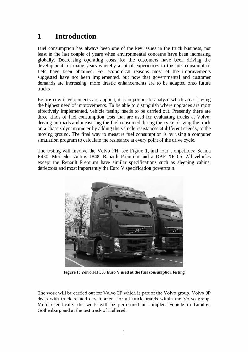
The testing will involve the Volvo FH, see Figure 1, and four competitors: Scania
R480, Mercedes Actros 1848, Renault Premium and a DAF XF105. All vehicles
except the Renault Premium have similar specifications such as sleeping cabins,
deflectors and most importantly the Euro V specification powertrain.
Figure 1: Volvo FH 500 Euro V used at the fuel consumption testing
The work will be carried out for Volvo 3P which is part of the Volvo group. Volvo 3P
deals with truck related development for all truck brands within the Volvo group.
More specifically the work will be performed at complete vehicle in Lundby,
Gothenburg and at the test track of Hällered.
CHALMERS, Applied Mechanics, Master’s Thesis 2010:18 2
2 Background
To construct more effective trucks than competitors, Volvo needs analysis of how
their trucks are performing compared to the main rivals. To be able to compare the
fuel consumption on an accurate scale, different tests of the Volvo FH as well as its
main competitors are carried out. The project will look into the test methods used to
get hold of the fuel consumption and finding drawbacks in using the particular
method.
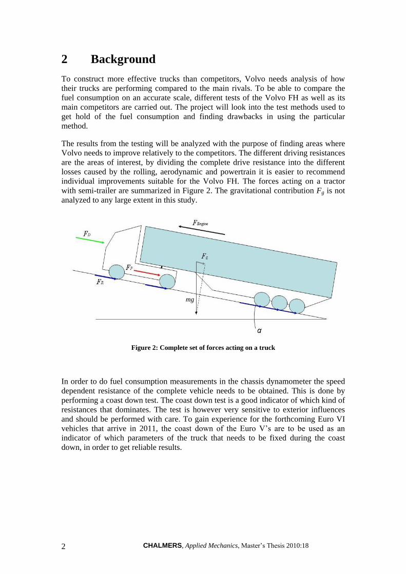
The results from the testing will be analyzed with the purpose of finding areas where
Volvo needs to improve relatively to the competitors. The different driving resistances
are the areas of interest, by dividing the complete drive resistance into the different
losses caused by the rolling, aerodynamic and powertrain it is easier to recommend
individual improvements suitable for the Volvo FH. The forces acting on a tractor
with semi-trailer are summarized in Figure 2. The gravitational contribution Fg is not
analyzed to any large extent in this study.
Figure 2: Complete set of forces acting on a truck
In order to do fuel consumption measurements in the chassis dynamometer the speed
dependent resistance of the complete vehicle needs to be obtained. This is done by
performing a coast down test. The coast down test is a good indicator of which kind of
resistances that dominates. The test is however very sensitive to exterior influences
and should be performed with care. To gain experience for the forthcoming Euro VI
vehicles that arrive in 2011, the coast down of the Euro V’s are to be used as an
indicator of which parameters of the truck that needs to be fixed during the coast
down, in order to get reliable results.
mg
3
3 Boundaries
The complexity and size of the project make it difficult to analyze emissions which
are one of the main purposes of this kind of vehicle testing. The emission analysis is
carried out parallel at Volvo Powertrain and does not require further attention. The
main reason why Euro V vehicles were used for the tests was for the emissions, but
the main attention of this report is on the drive resistances, the emissions should be
considered as a side step. Some of the duty cycles are however mainly interesting for
emissions whereby less attention to the fuel consumption results of these duty cycles
are seen.
Modifications of the tested vehicles were not possible to do due to the short time
period of this project, even if such measures would have been important in order to
achieve comparable results between the various trucks. Another reason was that the
competitor vehicles were borrowed and therefore no changes could be done.
Variations in fundamental parts such as tires were for example an area that undeniably
affected the resistances at the coast down test.
The analysis as well as the scope of the project is applicable on long haulage trucks,
consisting of a tractor with a semi-trailer. This is the most common configuration of
cargo trucks and therefore the greatest interest of improvement is found there. The
main results are nonetheless easy to apply onto other kinds of heavy vehicles.
CHALMERS, Applied Mechanics, Master’s Thesis 2010:18 4
4 Fuel Consumption Test Methods
Presently fuel consumption is measured in various ways in the vehicle industry. Some
ways are preferred when it comes to accuracy and some for their cost-effectiveness.
The most common methods are either real world road testing, chassis dynamometer
full vehicle simulation, computer simulation and engine bench measurement. Tests of
the first three methods have been performed and compared with each other in Chapter
5.
To be able to perform chassis dynamometer tests a load curve of the truck has to be
inserted into the computer. Load curves are created by measuring the driving force on
a complete truck for different speeds, one such test is called coast down test. The
vehicle is left on neutral gear for the entire speed interval of importance, by
continuously measuring the speed and time, from that accelerations and later on forces
can be calculated. The coast down testing also allows a lot of losses analyze to be
performed. Such as how much rolling and aerodynamic resistances contributes to
respectively, but also in what extent environmental parameters affect the results.
In order to more accurately investigate the coast down results a powertrain coast down
was performed. The test measures only the losses in the driveline and as a
consequence the two remaining resistances can more easily be distinguished.
The first two tests do not result in any fuel consumption read-outs, but they give an
insight of the driving resistances acting on the vehicle, which are affecting the fuel
consumption for the various configured trucks. Most importantly these tests act as the
base for the chassis dynamometer measurement.
The later part of this chapter is mainly focused on fuel consumption. The central part
in the report is to distinguish obvious differences between the test methods while the
comparison between competitors is a side track. The reason for this is the potentially
low repeatability of the tests; little care was taken to ensure equal conditions during
testing. The comparison between the test methods gives a clear indication of what
advantages and disadvantages that can be found, and hopefully help as a guide for
future testing of trucks. In the same time results comparisons between trucks can be
misguiding due to the unknown accuracy of test methods and the results dependency
on both truck and non-truck related factors.
4.1 Powertrain coast down
A powertrain coast down is a test conducted in order to find the speed dependent
resistance of the complete driveline. The rotational speed of the wheels are logged
with high frequency and used for calculating the wheel retardation.
5
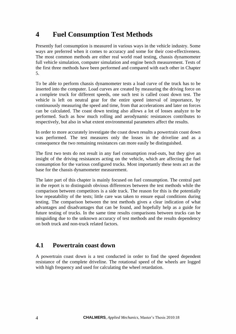
4.1.1 Powertrain coast down description
To perform the test, the rear of the truck was lifted from the ground, for safety reasons
the rear axle was both put on jack stands as well as lifted by an overhead crane, see
Figure 3. To measure purely powertrain losses the retarder has to be switched off,
moreover the wheel speed has to be measured on both wheels to prevent any frictional
difference in the bearings affecting the rotational speed. The differential distributes
the input speed to the wheel pair, but concentrates the speed to the side with less
resistance, as a consequence a small difference between wheel speeds can occur. The
average value of the two sides is finally used as the output speed in calculations.
Figure 3: Lifted vehicle at powertrain coast down test
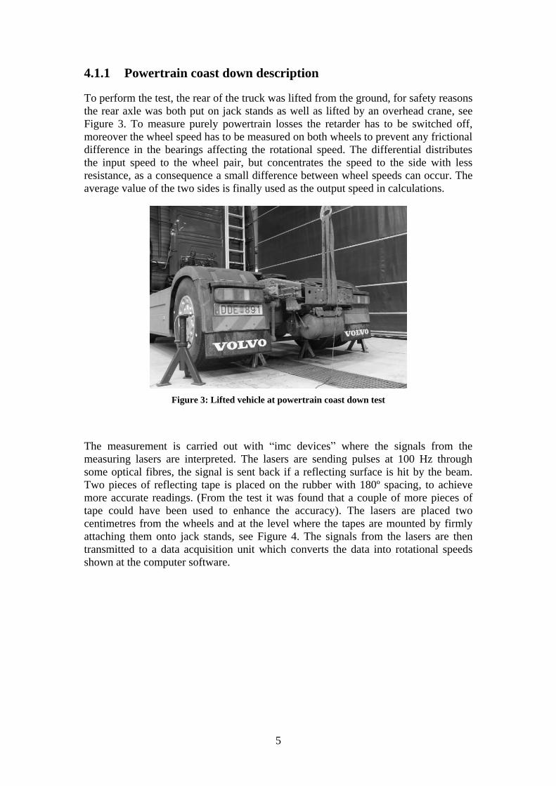
The measurement is carried out with “imc devices” where the signals from the
measuring lasers are interpreted. The lasers are sending pulses at 100 Hz through
some optical fibres, the signal is sent back if a reflecting surface is hit by the beam.
Two pieces of reflecting tape is placed on the rubber with 180º spacing, to achieve
more accurate readings. (From the test it was found that a couple of more pieces of
tape could have been used to enhance the accuracy). The lasers are placed two
centimetres from the wheels and at the level where the tapes are mounted by firmly
attaching them onto jack stands, see Figure 4. The signals from the lasers are then
transmitted to a data acquisition unit which converts the data into rotational speeds
shown at the computer software.
CHALMERS, Applied Mechanics, Master’s Thesis 2010:18 6
Figure 4: Laser mounting for powertrain coast down test
In order to run the engine in the workshop the exhaust was attached to a flexible
exhaust pipe. The ESP (Electronic Stability programme) and ABS (Anti-lock Braking
System) fuses were also disconnected just for precaution not to have any influence
from these systems.
To do the test the vehicle firstly needs to be propelled to 90 km/h (or close by), at this
speed the speed limiter cuts the fuel feeding and prohibit any speeds above 90 km/h. It
takes some time for the engine to regain the moment, and as a consequence the top
speeds are difficult to capture. As close to 90 km/h as possible the gearbox is put in
neutral. Before the gear change the logger program is triggered, all the extra data can
easily be cut out afterwards, the measurement is stopped when the low range gear is
connected at 16 km/h. When the low range gears connects the rotational speed of the
main shaft in the gearbox increases and raises the driving resistance.
4.1.2 Issues with powertrain coast down
The results from the measurement can for various reasons be inaccurate and/or wrong.
By listing the problems that might occur while testing, better knowledge on how to
interpret the results and improve future testing is obtained.
From the results a clear difference between cold and pre-heated components
was seen, the reason is the decreased viscosity of the various lubricants in the
powertrain. No temperatures in the gearbox or final drive were logged and
therefore it is difficult to accurately define whether the operating temperature
was reached or not. A decrease in transmission losses would most certainly be
achieved if the truck was warmed up to a higher extent.
7
Another factor was the inaccurate reading that only two pieces of tape
contributed to, when the wheels rotated slowly. The program worked in such a
way that if no signal was sent during the time interval the previous value was
stored instead. This can be seen in Appendix F 1 at low speeds where the
graphs become stair shaped.
In order to get a continuous curve the different runs are averaged and a
trendline based on a second order polynomial is used to describe the curve.
This trendline is later on used for calculation of the rotational speed difference,
by looking at the deceleration between two different speeds. In this method
some information is lost, but the trend should still be fairly accurate.
When calculating the moment at the wheels the inertia of all the components
has to be known. This information was collected from several sources, and
consequently different accuracies were used. The error should not be big
because the major contributors are the tires and those values were given from
the tire supplier Michelin for the specific tires used.
The inertia of the tires was approximated for a brand new set of rubber and
because material is consumed when the tires are worn the inertia could be
changed significantly.
Brake drag was not avoided in any extent, except that both wheels were
rotated to distinguish whether there were any big differences in resisting force.
It can be debated if the brake drag should be included in the calculation or not,
because at real driving some resisting force are caused by the brakes, the
magnitude is however difficult to recreate, because losses can be irregular
between tests.
The amount of oil in the gearbox as well as the final drive changes the splash
losses and no measurement was carried out to distinguish the amount, which
makes the test difficult to duplicate.
The bearing friction is decreased by having the rear axle lifted, and not having
any extra loading on the bearing surface.
4.1.3 The powertrain test
In order to perform the powertrain coast down test a Volvo FH13 was used with
similar specifications as the one used later on at the coast down test, see Figure 5.
Firstly a test where all the components were cold was conducted. Five runs were
carried out with this condition, but only four of them were valid due to a late start of
data logging in one of them. The same tendency could be seen in all the valid runs,
see Appendix F 1. The weather prior to the drive into the workshop was -2 ºC. Due to
some preparation time inside the workshop before the actual measurement took place
a slight increase in component temperature can be expected.
CHALMERS, Applied Mechanics, Master’s Thesis 2010:18 8
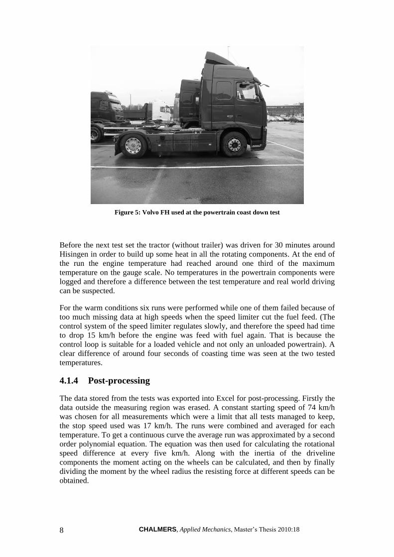
Figure 5: Volvo FH used at the powertrain coast down test
Before the next test set the tractor (without trailer) was driven for 30 minutes around
Hisingen in order to build up some heat in all the rotating components. At the end of
the run the engine temperature had reached around one third of the maximum
temperature on the gauge scale. No temperatures in the powertrain components were
logged and therefore a difference between the test temperature and real world driving
can be suspected.
For the warm conditions six runs were performed while one of them failed because of
too much missing data at high speeds when the speed limiter cut the fuel feed. (The
control system of the speed limiter regulates slowly, and therefore the speed had time
to drop 15 km/h before the engine was feed with fuel again. That is because the
control loop is suitable for a loaded vehicle and not only an unloaded powertrain). A
clear difference of around four seconds of coasting time was seen at the two tested
temperatures.
4.1.4 Post-processing
The data stored from the tests was exported into Excel for post-processing. Firstly the
data outside the measuring region was erased. A constant starting speed of 74 km/h
was chosen for all measurements which were a limit that all tests managed to keep,
the stop speed used was 17 km/h. The runs were combined and averaged for each
temperature. To get a continuous curve the average run was approximated by a second
order polynomial equation. The equation was then used for calculating the rotational
speed difference at every five km/h. Along with the inertia of the driveline
components the moment acting on the wheels can be calculated, and then by finally
dividing the moment by the wheel radius the resisting force at different speeds can be
obtained.
9
The inertia of the various powertrain components were collected from different
departments at Volvo group and probably have various reliabilities. The inertia of
tires was given from Michelin for their specific model XDA2 which are the main
contributors of the inertia. The driveshaft’s, differential gear’s, (with gear ratio 2.64:1)
and pinion’s inertia was given from department: axle engineering in France. The
gearbox inertia of the I-shift transmission in neutral and with the high range gear
connected was given from department: drivelines and hybrids. The propeller shaft C
2055’s inertia was given from department: driveline subsystems. The brake disc and
wheel hub were measured in size and approximated as cylinders of different sizes in
order to calculate their inertia, see Appendix H.
The inertia times the change in rotational speed is basically proportional to the
frictional losses and the splash losses. The frictional losses can be divided into
rubbing between gear wheels, (in this case that is mostly the final drive, because it is
heavily pre-tensioned), and bearing friction. Most bearings in the powertrain are of
conical type in order to withstand the axial loads caused by helical and hypoid gears.
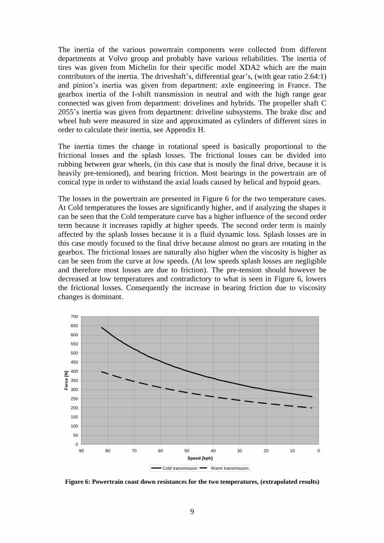
The losses in the powertrain are presented in Figure 6 for the two temperature cases.
At Cold temperatures the losses are significantly higher, and if analyzing the shapes it
can be seen that the Cold temperature curve has a higher influence of the second order
term because it increases rapidly at higher speeds. The second order term is mainly
affected by the splash losses because it is a fluid dynamic loss. Splash losses are in
this case mostly focused to the final drive because almost no gears are rotating in the
gearbox. The frictional losses are naturally also higher when the viscosity is higher as
can be seen from the curve at low speeds. (At low speeds splash losses are negligible
and therefore most losses are due to friction). The pre-tension should however be
decreased at low temperatures and contradictory to what is seen in Figure 6, lowers
the frictional losses. Consequently the increase in bearing friction due to viscosity
changes is dominant.
0
50
100
150
200
250
300
350
400
450
500
550
600
650
700
0102030405060708090
Speed [kph]
Fo
rce
[N
]
Cold transmission Warm transmission
Figure 6: Powertrain coast down resistances for the two temperatures, (extrapolated results)
CHALMERS, Applied Mechanics, Master’s Thesis 2010:18 10
4.2 Coast down test
To improve fuel consumption of trucks driving resistances must be kept low. The
main losses are divided into aerodynamic resistance, rolling resistance and resistance
due to gradients. While the first three losses are much dependent on how efficient the
vehicle is, the last one is mainly dependent on the terrain. The main interests here are
therefore to decrease the first three losses. The most accurate way is by measuring the
actual fuel consumption for a specific cycle on the road. Repeatability of road tests is
however low and it is not feasible to perform for all different combinations, of cabins,
trailers, engines, transmissions etc. A far more attractive approach is to run the
vehicles inside, in-house in a chassis dynamometer. The complication is to get the
actual resistance at different vehicle speeds for the complete vehicle. One way of
measuring the combined resistances at varying vehicle speeds is performing a coast
down test.
4.2.1 Coast down description
The coast down is a difficult test to perform if accurate and repeatable results are to be
obtained, parallel to that it is both time and cost consuming, especially if competitor
vehicles are to be rented or bought for comparison. The basic principle is to measure
for how long the vehicle is able to coast from a certain speed. A starting speed a bit
above 85 km/h1 is sufficient for a truck because the maximum allowed speed is 80
km/h. When the vehicle has reached the starting speed and a sufficiently long straight,
(800m is sufficient), the gearlever is put into neutral position. The vehicle is now
coasting down the straight and the friction from moving components along with the
approaching air decelerates the vehicle’s speed. During the deceleration the time and
speed are being measured.
For good accuracy the speed is obtained from a 5th
wheel mounted onto the truck. The
5th
wheel is mounted tight to the vehicle but is allowed to follow the roads unevenness
with help of a spring and damper. It’s important that the wheel has contact with the
ground at all conditions and preferably not varying the contact load much, because it
changes the effective rolling radius of the tire. The 5th
wheel has to be calibrated prior
to the measurement in order to find the calibration factor, which equals the amount of
sensing pulses per meter road. To get the vehicle speed the amount of pulses per
second is divided by the calibration factor.
The coast down course has to be straight and flat to exclude side forces and the
influence of gradients. Moreover the surface needs to be dry in order not to exaggerate
the rolling resistance contribution. A day with absence of wind is also preferred so
that a consistent measurement is conducted and variations in aerodynamic force are
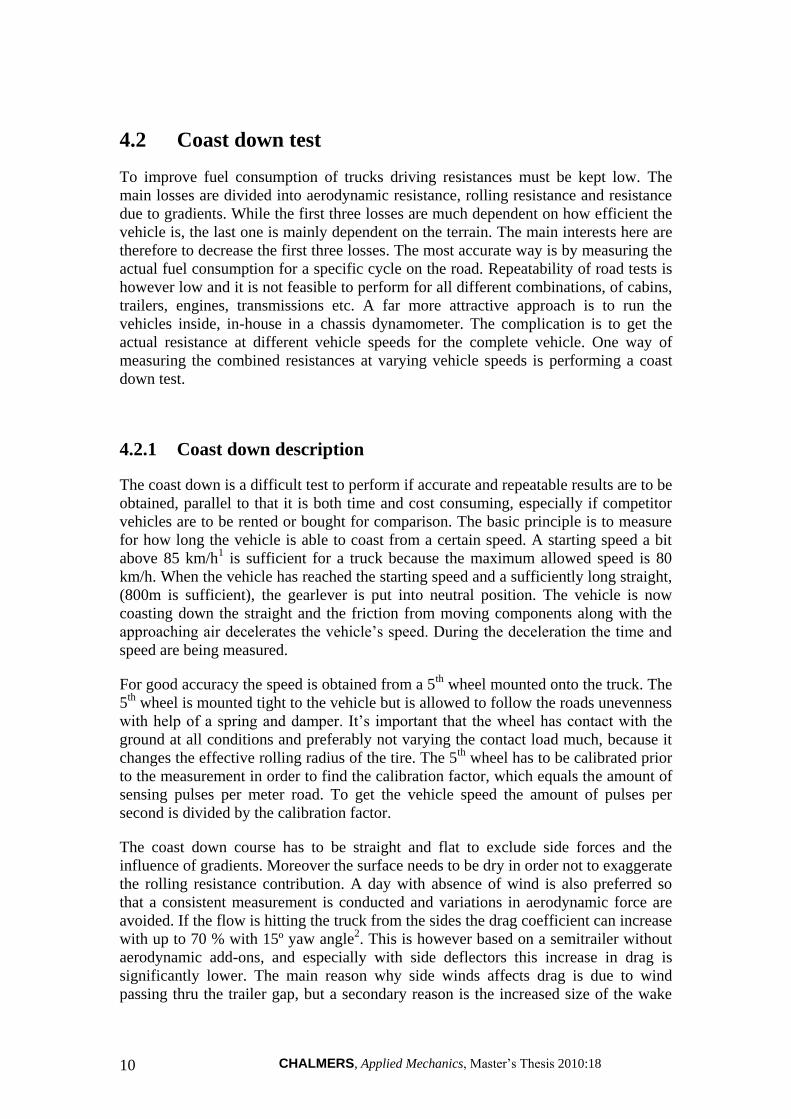
avoided. If the flow is hitting the truck from the sides the drag coefficient can increase
with up to 70 % with 15º yaw angle2. This is however based on a semitrailer without
aerodynamic add-ons, and especially with side deflectors this increase in drag is
significantly lower. The main reason why side winds affects drag is due to wind
passing thru the trailer gap, but a secondary reason is the increased size of the wake
11
region, see Figure 7. Lastly it should be noted that even the frontal area increases with
a slightly increases with a slightly angled head wind.
Figure 7: Side wind motion around semitrailer, plus wake region.
Normally a heavy truck is coasting for quite a while, resulting in a number of required
runs down the straight in order to complete the sequence. To get a continuous data
sequence the next run must be started with a bit of overlap in speed. Normally the
procedure stops when the speed is reaching 10 km/h because then more factors comes
into play. For Volvo trucks the limit is a bit higher because the low range neutral gear
automatically engages below 16 km/h and changes the driveline force significantly,
(this speed can vary between manufacturers and gearbox type).
4.2.2 Issues with coast down
To achieve reliable test results some different conditions must be met. In most cases
the procedure to go thru all faults is very time consuming and therefore most of them
can be neglected, the result can however be very misleading in the worst scenarios.
Temperature of all components must be kept constant between tests, for
example oil temperatures of transmission and rear axle have to be relatively
constant to achieve comparable results. If significant temperature differences
occur the viscosity difference of the oil will result in varying driveline
resistances.
Temperature differences in the tires can also affect the results, because friction
increases when tires are warm. In order to quickly build up temperature in the
tire the hysteresis must be high, which is achieved by driving fast and/or at
bumpy roads.
Road conditions are also affecting the results partly because water on the road
sticks to the rubber and increases rolling resistance. But also because the water
acts as coolant and thereby changes the bounding force between the rubber
and the asphalt, (decreasing hysteresis).
CHALMERS, Applied Mechanics, Master’s Thesis 2010:18 12
Winds are also affecting the results. Head- and tailwind obviously change the
aerodynamic resistance, but side winds not only increases the relative speed it
also results in higher drag coefficient. Especially sensitive to side winds are
trucks with gaps between the tractor and trailer, (such as the semi-trailer).
Headwinds above 2 m/s are usually a level where significant influence on the
results is occuring.
If different roads are used between tests the results might be affected by
different adhesion factors, and consequently different rolling resistances. The
different types of asphalt can also vary the up and down movements of the
wheels and thereby increase the losses due to energy absorption in the
suspension and tires.
Road inclinations are also an issue affecting the force required to propel the
vehicle. The height difference between start and finish point of measurement
is important to keep constant, but also the shape of the course can affect, as if
the track is shaped as a hammock. On Hällered the straights varies in height
with around 1 m. To compensate for this the height above sea level can be
continuously measured to be able to subtract that contribution.
The right amount of oil in the gearbox is also important to avoid non-
comparable splash losses, between different trucks.
Brake pads and shoes must be sufficiently worn-in to present realistic surface
friction. Worn brake pads also have a tendency to move the rubbing friction
surface away from the disc due to more unevenness at the friction surface, and
thereby decrease the rolling resistance.
Tire pressure must be accurately checked and filled at a standard temperature.
If the tires were checked at low temperature the pressure will show lower
values than for high temperature measurements.
In winters snow on the surface of the truck can drastically increase the viscous
forces, and especially at the large trailer surface area. In summers and winters
dirt can also increase the surface friction, whereby a clean and dry vehicle is
preferred.
The surrounding air pressure also affects the aerodynamic force factor by
changing the air density and is around 7 % higher at -5ºC relative to +15ºC,
and therefore the aerodynamic force has a larger contribution at cold weathers.
The trucks utilize air suspensions and can consequently change ride heights.
The comparison between different vehicles is therefore much dependent on
correctly set ride heights.
Correctly adjusted roof and side deflectors are necessary in order to have
similar aerodynamic conditions for the different vehicles tested. That is a
smooth transition between the tractor and trailer.
Similar tires are needed to achieve comparable results between different
vehicles. The tire brand, tire size, the tire pattern as well as the filler content of
silica-silane as replacement for carbon black are factors needed to be kept
constant to have comparable losses between trucks. The wear of the tire is
another factor influencing the rolling resistance coefficient, up to 20 % lower
for worn tires, than for new ones.
13
If the truck is not sufficiently worn-in there might be rolling resistance related
losses from, suspensions that are not sufficiently seated and consequently have
the wrong wheel angles or just a lot of energy absorption. Transmission parts
are also required to be worn-in to represent actual friction losses.
Toe-in can significantly increase rolling resistance, by having high toe-in
values the vehicle becomes more stable whereby some manufacturers tends to
use high values. The wheel angles can also be distorted by severe contacts to
heavy obstacles. In order to have reliable comparisons these angles should be
kept at the same level for all vehicles or at the manufacturer specified values.
Vertical movement of the truck due to road unevenness is also affecting the
results, because forward motion is transferred into vertical motion and lost in
the dampers as heat. But the results can also be spoiled if the road unevenness
changes the effective rolling radius of the 5th
wheel tire and consequently
changing the amount of pulses per wheel revolution.
The aerodynamics of the truck is changed by removing some of the radiator
panels. The absences of the panels are due to mountings of the 5th
wheel. It is
hard to predict whether or not the panels give any clear change in drag
coefficient, but they do not only change the shape they also allow more air to
pass through the radiator, and consequently the engine might get colder,
especially at winters. This is however not affecting the coast down results.
4.2.3 Test preparations
Before the coast down test a number of vehicle preparations are required. Most
importantly the 5th
wheel must be firmly mounted to the body, either at the front on
the beams behind the radiator grille, or to mount the wheel behind the tractor, as long
as it moves freely from the trailer. For the trailer used, there is not enough space
between the trailer and the tractor, whereby the mounting has to be in front. For most
trucks the towing hook is used to hold the 5th
wheel armature. The important aspect is
to insure that the wheel is not able to move relative to the ground, and a stiff mounting
is therefore required.
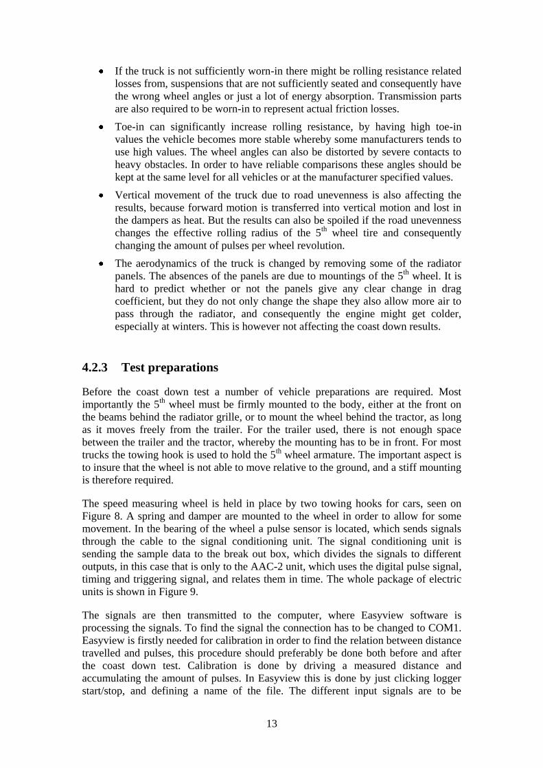
The speed measuring wheel is held in place by two towing hooks for cars, seen on
Figure 8. A spring and damper are mounted to the wheel in order to allow for some
movement. In the bearing of the wheel a pulse sensor is located, which sends signals
through the cable to the signal conditioning unit. The signal conditioning unit is
sending the sample data to the break out box, which divides the signals to different
outputs, in this case that is only to the AAC-2 unit, which uses the digital pulse signal,
timing and triggering signal, and relates them in time. The whole package of electric
units is shown in Figure 9.
The signals are then transmitted to the computer, where Easyview software is
processing the signals. To find the signal the connection has to be changed to COM1.
Easyview is firstly needed for calibration in order to find the relation between distance
travelled and pulses, this procedure should preferably be done both before and after
the coast down test. Calibration is done by driving a measured distance and
accumulating the amount of pulses. In Easyview this is done by just clicking logger
start/stop, and defining a name of the file. The different input signals are to be
CHALMERS, Applied Mechanics, Master’s Thesis 2010:18 14
defined; number 3 is the trigger signal, while the wheel speed sensor is number 25.
The wheel speed has to be set to accumulated measurement, all other parameters are
using the preset values. The sampling rate might have to be changed to 10 Hz, (if this
is not changed automatically). When pressing Finish the sampling will start, to
observe the measurement the green voltage meter can be used. When the finishing
line is reached the value is stored and used for calculating the calibration factor by
dividing the value by the distance travelled.
Figure 8: 5th
wheel and mounting plates on the Scania R-series
Next step is to start the measurement, this is done by pressing Logger Start, by using
the previously defined parameters the only things to change is the wheel pulses
sampling. Instead of accumulated, reset pulses are to be used, the rest is just to leave
unchanged. When pressing Finish the logger will start calculating pulses, the real
measurement will however not start until the trigger has been pushed. In order to stop
the sampling the trigger is used to indicate when this will occur. The continuous
sampling is stopped by pressing Logger Stop. The file can now be saved and exported
as a txt file. The whole measurement range has to be exported and this is done by
changing the view to see the complete sample and then export.
15
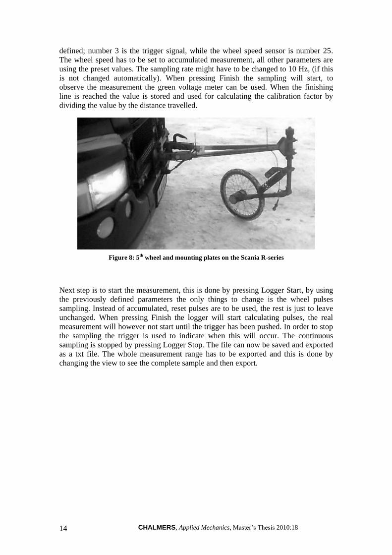
Figure 9: Measuring equipment for 5th
wheel and trigger
Finally the components are all connected and driven by the 24V auxiliary system of
the truck. As a result a DC/DC converter has to be applied to produce the 12V needed
for the AAC-2. The other components use the power supply box as source. From that
box there is one 12V output that is used to provide the laptop with the right voltage.
4.2.4 Coast down post-processing
The data accumulated in Easyview is exported as a txt file in order to open the data in
Excel. The data file is cut in Excel to only show the values of where the measurement
occurred, for simplification all runs were arranged after the same starting speed of
measurement. The data string was ended when speeds dropped below 16 km/h, in
order to avoid the low range neutral gear affecting the resistance. After the first data
clean-up the runs are plotted in order to find individual runs diverging, and in worst
case exclude them from the averaging.
The different runs that are significant are then averaged for both straights, the data are
then converted from pulses into speeds by dividing it with the calibration factor. The
results from the two straights are then combined in order to lessen the effect of wind
and road inclination differences. The time is now plotted relative to speed in order to
make a curve fit where a second order polynomial equation is describing the speed
relative to time. The equation is now used to calculate the time elapsed between some
vehicle speeds. The speed difference divided by the elapsed time is equal to the
deceleration. The force acting on the truck at a certain speed is then obtained by
multiplying the acceleration with the mass. Force versus speed can now be presented
by a second order polynomial, the equation contains three terms that are describing
the load curve used in the chassis dynamometer.
CHALMERS, Applied Mechanics, Master’s Thesis 2010:18 16
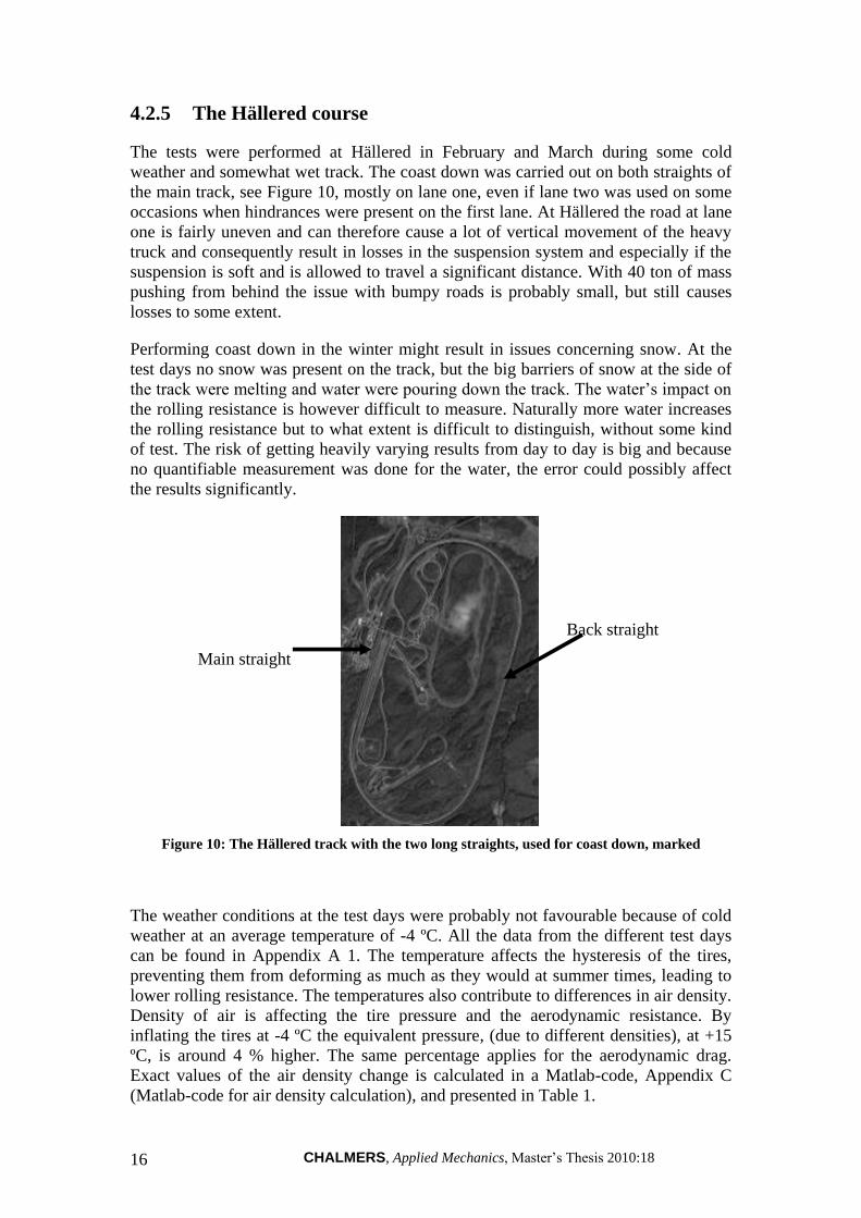
4.2.5 The Hällered course
The tests were performed at Hällered in February and March during some cold
weather and somewhat wet track. The coast down was carried out on both straights of
the main track, see Figure 10, mostly on lane one, even if lane two was used on some
occasions when hindrances were present on the first lane. At Hällered the road at lane
one is fairly uneven and can therefore cause a lot of vertical movement of the heavy
truck and consequently result in losses in the suspension system and especially if the
suspension is soft and is allowed to travel a significant distance. With 40 ton of mass
pushing from behind the issue with bumpy roads is probably small, but still causes
losses to some extent.
Performing coast down in the winter might result in issues concerning snow. At the
test days no snow was present on the track, but the big barriers of snow at the side of
the track were melting and water were pouring down the track. The water’s impact on
the rolling resistance is however difficult to measure. Naturally more water increases
the rolling resistance but to what extent is difficult to distinguish, without some kind
of test. The risk of getting heavily varying results from day to day is big and because
no quantifiable measurement was done for the water, the error could possibly affect
the results significantly.
Figure 10: The Hällered track with the two long straights, used for coast down, marked
The weather conditions at the test days were probably not favourable because of cold
weather at an average temperature of -4 ºC. All the data from the different test days
can be found in Appendix A 1. The temperature affects the hysteresis of the tires,
preventing them from deforming as much as they would at summer times, leading to
lower rolling resistance. The temperatures also contribute to differences in air density.
Density of air is affecting the tire pressure and the aerodynamic resistance. By
inflating the tires at -4 ºC the equivalent pressure, (due to different densities), at +15
ºC, is around 4 % higher. The same percentage applies for the aerodynamic drag.
Exact values of the air density change is calculated in a Matlab-code, Appendix C
(Matlab-code for air density calculation), and presented in Table 1.
Back straight
Main straight
17
Table 1: Air densities at the different tests
Vehicle:
Air density at test day
[kg/m3]
Percentage difference to
reference vehicle [%]
Volvo FH at 15 ºC, reference3 1.228 -
Scania R-series 1.283 4.3
Mercedes Actros 1.280 4.1
Volvo FH 1.294 5.1
Renault Premium 1.268 3.1
DAF XF 1.268 3.2
The wind is shown in Appendix A 1 and the direction is referred to angles clockwise
counted from north winds, which are 0º. The Hällered main track straights are
directed at 18º from north direction4. The wind is naturally affecting the aerodynamic
resistance, but by averaging the results from both straights the influence of wind can
to some extent be cancelled. Worst case is if the wind is hitting the truck from the side
resulting in an increase of drag at both straights.
4.2.6 The coast down tests
Before the testing of each vehicle some vehicle specifications had to be stored. Not all
information was possible to log because the vehicle was borrowed, but the major
contributor to force differences are stored, such as weight, aerodynamic spoilers and
vehicle tires. The information is saved in order to easily compare and later on
conclude what parameters caused the differences in the results. The vehicle
specifications are also important for future testing and follow-ups. Most of the data is
presented in appendix, while more abstract devices, such as side skirts are described
in the text for each vehicle.
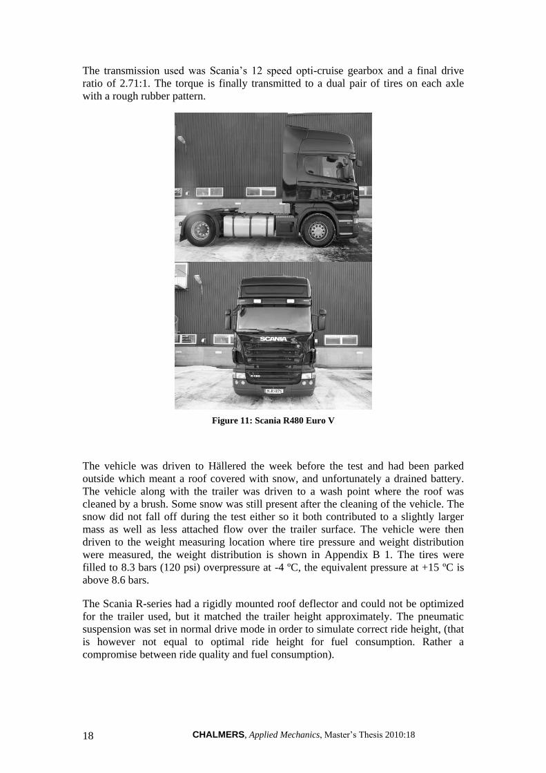
4.2.6.1 Scania coast down
The Scania R480 used in the coast down test is equipped with a full size sleeper cabin
and therefore does not need any large roof deflector in order to create a smooth
transition between the cabin and trailer. The steep front can however worsen the
aerodynamics, because of a larger region where stagnation pressure is reached. The
vehicle also utilizes a lot of add-ons such as side and front mirrors and sunvisor,
which does not improve the flow around the front of the vehicle, the shape can be
seen in Figure 11.
CHALMERS, Applied Mechanics, Master’s Thesis 2010:18 18
The transmission used was Scania’s 12 speed opti-cruise gearbox and a final drive
ratio of 2.71:1. The torque is finally transmitted to a dual pair of tires on each axle
with a rough rubber pattern.
Figure 11: Scania R480 Euro V
The vehicle was driven to Hällered the week before the test and had been parked
outside which meant a roof covered with snow, and unfortunately a drained battery.
The vehicle along with the trailer was driven to a wash point where the roof was
cleaned by a brush. Some snow was still present after the cleaning of the vehicle. The
snow did not fall off during the test either so it both contributed to a slightly larger
mass as well as less attached flow over the trailer surface. The vehicle were then
driven to the weight measuring location where tire pressure and weight distribution
were measured, the weight distribution is shown in Appendix B 1. The tires were
filled to 8.3 bars (120 psi) overpressure at -4 ºC, the equivalent pressure at +15 ºC is
above 8.6 bars.
The Scania R-series had a rigidly mounted roof deflector and could not be optimized
for the trailer used, but it matched the trailer height approximately. The pneumatic
suspension was set in normal drive mode in order to simulate correct ride height, (that
is however not equal to optimal ride height for fuel consumption. Rather a
compromise between ride quality and fuel consumption).
19
To achieve reliable results from the coast down the vehicle should be sufficiently
worn-in, in the Scania case the vehicle only had run for about 1000 km which is not
enough to fully allow all bearing surfaces or gearwheel contacts to embed. But brake
pads and wheel angles are assumed to be close to ideal because of the short time of
vehicle use, and thereby less time for uneven wear of pads or distortion of the
suspension. The tires were also of a rough model with very little wear and probably
affected the rolling resistance badly, the model was Bridgestone M 729, a tire suitable
for winters.
When performing coast downs a significant amount of warm-up driving is required in
order to build-up normal operating temperature in the driveline components and tires.
Normally the temperatures in the driveline would have been monitored but due to the
fact that the vehicle was borrowed none such sensors were fitted. After one and a half
hour of warm-up the 5th
wheel was calibrated to a fixed distance in order to relate
number of pulses to distance rolled.
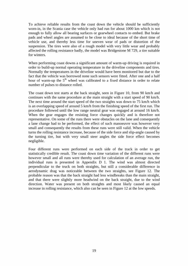
The coast down test starts at the back straight, seen in Figure 10, from 90 km/h and
continues with the same procedure at the main straight with a start speed of 90 km/h.
The next time around the start speed of the two straights was down to 75 km/h which
is an overlapping speed of around 5 km/h from the finishing speed of the first run. The
procedure followed until the low range neutral gear was engaged at around 16 km/h.
When the gear engages the resisting force changes quickly and is therefore not
representative. On some of the runs there were obstacles on the lane and consequently
a lane change had to be performed, the effect of such manoeuvre was however very
small and consequently the results from these runs were still valid. When the vehicle
turns the rolling resistance increase, because of the side force and slip-angle caused by
the turning tire, but with very small steer angles the side force effect becomes
negligible.
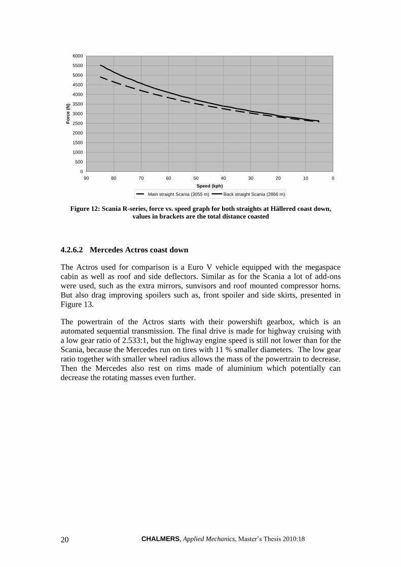
Four different runs were performed on each side of the track in order to get
statistically credible result. The coast down time variation of the different runs were
however small and all runs were thereby used for calculation of an average run, the
individual runs is presented in Appendix D 1. The wind was almost directed
perpendicular to the truck on both straights, but still a considerable difference in
aerodynamic drag was noticeable between the two straights, see Figure 12. The
probable reason was that the back straight had less windbreaks than the main straight,
and that there were slightly more headwind on the back straight, due to the wind
direction. Water was present on both straights and most likely caused an equal
increase in rolling resistance, which also can be seen in Figure 12 at the low speeds.
CHALMERS, Applied Mechanics, Master’s Thesis 2010:18 20
0
500
1000
1500
2000
2500
3000
3500
4000
4500
5000
5500
6000
0102030405060708090
Speed (kph)
Fo
rce
(N
)
Main straight Scania (3055 m) Back straight Scania (2866 m)
Figure 12: Scania R-series, force vs. speed graph for both straights at Hällered coast down,
values in brackets are the total distance coasted
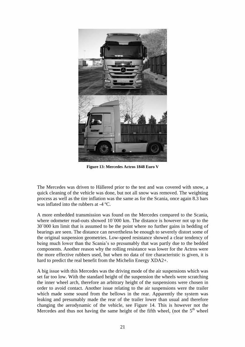
4.2.6.2 Mercedes Actros coast down
The Actros used for comparison is a Euro V vehicle equipped with the megaspace
cabin as well as roof and side deflectors. Similar as for the Scania a lot of add-ons
were used, such as the extra mirrors, sunvisors and roof mounted compressor horns.
But also drag improving spoilers such as, front spoiler and side skirts, presented in
Figure 13.
The powertrain of the Actros starts with their powershift gearbox, which is an
automated sequential transmission. The final drive is made for highway cruising with
a low gear ratio of 2.533:1, but the highway engine speed is still not lower than for the
Scania, because the Mercedes run on tires with 11 % smaller diameters. The low gear
ratio together with smaller wheel radius allows the mass of the powertrain to decrease.
Then the Mercedes also rest on rims made of aluminium which potentially can
decrease the rotating masses even further.
21
Figure 13: Mercedes Actros 1848 Euro V
The Mercedes was driven to Hällered prior to the test and was covered with snow, a
quick cleaning of the vehicle was done, but not all snow was removed. The weighting
process as well as the tire inflation was the same as for the Scania, once again 8.3 bars
was inflated into the rubbers at -4 ºC.
A more embedded transmission was found on the Mercedes compared to the Scania,
where odometer read-outs showed 10´000 km. The distance is however not up to the
30´000 km limit that is assumed to be the point where no further gains in bedding of
bearings are seen. The distance can nevertheless be enough to severely distort some of
the original suspension geometries. Low-speed resistance showed a clear tendency of
being much lower than the Scania’s so presumably that was partly due to the bedded
components. Another reason why the rolling resistance was lower for the Actros were
the more effective rubbers used, but when no data of tire characteristic is given, it is
hard to predict the real benefit from the Michelin Energy XDA2+.
A big issue with this Mercedes was the driving mode of the air suspensions which was
set far too low. With the standard height of the suspension the wheels were scratching
the inner wheel arch, therefore an arbitrary height of the suspensions were chosen in
order to avoid contact. Another issue relating to the air suspensions were the trailer
which made some sound from the bellows in the rear. Apparently the system was
leaking and presumably made the rear of the trailer lower than usual and therefore
changing the aerodynamic of the vehicle, see Figure 14. This is however not the
Mercedes and thus not having the same height of the fifth wheel, (not the 5th
wheel
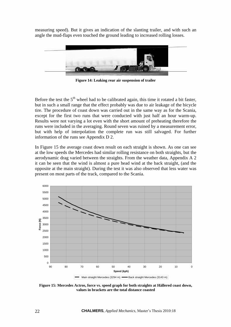
CHALMERS, Applied Mechanics, Master’s Thesis 2010:18 22
measuring speed). But it gives an indication of the slanting trailer, and with such an
angle the mud-flaps even touched the ground leading to increased rolling losses.
Figure 14: Leaking rear air suspension of trailer
Before the test the 5th
wheel had to be calibrated again, this time it rotated a bit faster,
but in such a small range that the effect probably was due to air leakage of the bicycle
tire. The procedure of coast down was carried out in the same way as for the Scania,
except for the first two runs that were conducted with just half an hour warm-up.
Results were not varying a lot even with the short amount of preheating therefore the
runs were included in the averaging. Round seven was ruined by a measurement error,
but with help of interpolation the complete run was still salvaged. For further
information of the runs see Appendix D 2.
In Figure 15 the average coast down result on each straight is shown. As one can see
at the low speeds the Mercedes had similar rolling resistance on both straights, but the
aerodynamic drag varied between the straights. From the weather data, Appendix A 2
it can be seen that the wind is almost a pure head wind at the back straight, (and the
opposite at the main straight). During the test it was also observed that less water was
present on most parts of the track, compared to the Scania.
0
500
1000
1500
2000
2500
3000
3500
4000
4500
5000
5500
6000
0102030405060708090
Speed (kph)
Fo
rce
(N
)
Main straight Mercedes (3294 m) Back straight Mercedes (3143 m)
Figure 15: Mercedes Actros, force vs. speed graph for both straights at Hällered coast down,
values in brackets are the total distance coasted
23
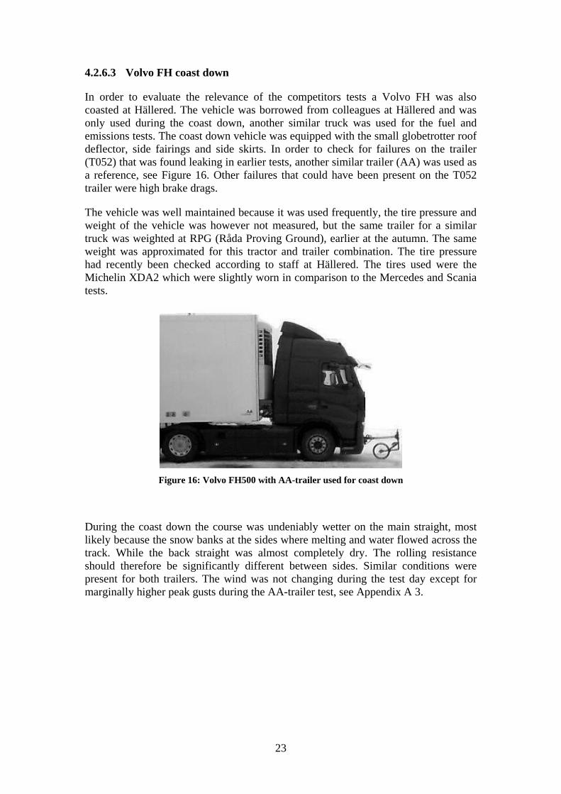
4.2.6.3 Volvo FH coast down
In order to evaluate the relevance of the competitors tests a Volvo FH was also
coasted at Hällered. The vehicle was borrowed from colleagues at Hällered and was
only used during the coast down, another similar truck was used for the fuel and
emissions tests. The coast down vehicle was equipped with the small globetrotter roof
deflector, side fairings and side skirts. In order to check for failures on the trailer
(T052) that was found leaking in earlier tests, another similar trailer (AA) was used as
a reference, see Figure 16. Other failures that could have been present on the T052
trailer were high brake drags.
The vehicle was well maintained because it was used frequently, the tire pressure and
weight of the vehicle was however not measured, but the same trailer for a similar
truck was weighted at RPG (Råda Proving Ground), earlier at the autumn. The same
weight was approximated for this tractor and trailer combination. The tire pressure
had recently been checked according to staff at Hällered. The tires used were the
Michelin XDA2 which were slightly worn in comparison to the Mercedes and Scania
tests.
Figure 16: Volvo FH500 with AA-trailer used for coast down
During the coast down the course was undeniably wetter on the main straight, most
likely because the snow banks at the sides where melting and water flowed across the
track. While the back straight was almost completely dry. The rolling resistance
should therefore be significantly different between sides. Similar conditions were
present for both trailers. The wind was not changing during the test day except for
marginally higher peak gusts during the AA-trailer test, see Appendix A 3.
CHALMERS, Applied Mechanics, Master’s Thesis 2010:18 24
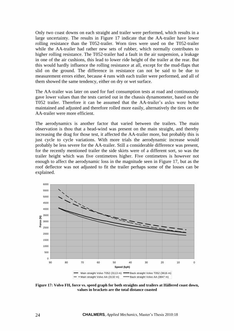
Only two coast downs on each straight and trailer were performed, which results in a
large uncertainty. The results in Figure 17 indicate that the AA-trailer have lower
rolling resistance than the T052-trailer. Worn tires were used on the T052-trailer
while the AA-trailer had rather new sets of rubber, which normally contributes to
higher rolling resistance. The T052-trailer had a fault in the air suspension, a leakage
in one of the air cushions, this lead to lower ride height of the trailer at the rear. But
this would hardly influence the rolling resistance at all, except for the mud-flaps that
slid on the ground. The difference in resistance can not be said to be due to
measurement errors either, because 4 runs with each trailer were performed, and all of
them showed the same tendency, either on dry or wet surface.
The AA-trailer was later on used for fuel consumption tests at road and continuously
gave lower values than the tests carried out in the chassis dynamometer, based on the
T052 trailer. Therefore it can be assumed that the AA-trailer’s axles were better
maintained and adjusted and therefore rolled more easily, alternatively the tires on the
AA-trailer were more efficient.
The aerodynamics is another factor that varied between the trailers. The main
observation is thou that a head-wind was present on the main straight, and thereby
increasing the drag for those test, it affected the AA-trailer more, but probably this is
just cycle to cycle variations. With more trials the aerodynamic increase would
probably be less severe for the AA-trailer. Still a considerable difference was present,
for the recently mentioned trailer the side skirts were of a different sort, so was the
trailer height which was five centimetres higher. Five centimetres is however not
enough to affect the aerodynamic loss in the magnitude seen in Figure 17, but as the
roof deflector was not adjusted to fit the trailer perhaps some of the losses can be
explained.
0
500
1000
1500
2000
2500
3000
3500
4000
4500
5000
5500
6000
0102030405060708090
Speed (kph)
Fo
rce
(N
)
Main straight Volvo T052 (3113 m) Back straight Volvo T052 (3616 m)
Main straight Volvo AA (3132 m) Back straight Volvo AA (3847 m)
Figure 17: Volvo FH, force vs. speed graph for both straights and trailers at Hällered coast down,
values in brackets are the total distance coasted
25
4.2.6.4 Renault Premium coast down
A Renault Premium was sent to Lundby from Lyon to also participate in the test. The
vehicle is hardly the same type as the other full size long-haulage trucks, and thereby
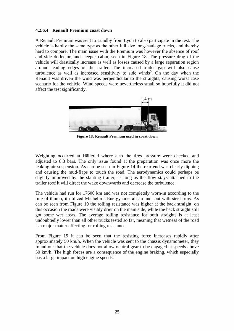
hard to compare. The main issue with the Premium was however the absence of roof
and side deflector, and sleeper cabin, seen in Figure 18. The pressure drag of the
vehicle will drastically increase as well as losses caused by a large separation region
around leading edges of the trailer. The increased trailer gap will also cause
turbulence as well as increased sensitivity to side winds5. On the day when the
Renault was driven the wind was perpendicular to the straights, causing worst case
scenario for the vehicle. Wind speeds were nevertheless small so hopefully it did not
affect the test significantly.
Figure 18: Renault Premium used in coast down
Weighting occurred at Hällered where also the tires pressure were checked and
adjusted to 8.3 bars. The only issue found at the preparation was once more the
leaking air suspension. As can be seen in Figure 14 the rear end was clearly dipping
and causing the mud-flaps to touch the road. The aerodynamics could perhaps be
slightly improved by the slanting trailer, as long as the flow stays attached to the
trailer roof it will direct the wake downwards and decrease the turbulence.
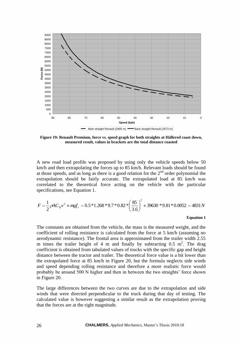
The vehicle had run for 17600 km and was not completely worn-in according to the
rule of thumb, it utilized Michelin’s Energy tires all around, but with steel rims. As
can be seen from Figure 19 the rolling resistance was higher at the back straight, on
this occasion the roads were visibly drier on the main side, while the back straight still
got some wet areas. The average rolling resistance for both straights is at least
undoubtedly lower than all other trucks tested so far, meaning that wetness of the road
is a major matter affecting for rolling resistance.
From Figure 19 it can be seen that the resisting force increases rapidly after
approximately 50 km/h. When the vehicle was sent to the chassis dynamometer, they
found out that the vehicle does not allow neutral gear to be engaged at speeds above
50 km/h. The high forces are a consequence of the engine braking, which especially
has a large impact on high engine speeds.
CHALMERS, Applied Mechanics, Master’s Thesis 2010:18 26
0
500
1000
1500
2000
2500
3000
3500
4000
4500
5000
5500
6000
6500
7000
7500
8000
8500
9000
0102030405060708090
Speed (kph)
Fo
rce
(N
)
Main straight Renault (2995 m) Back straight Renault (2673 m)
Figure 19: Renault Premium, force vs. speed graph for both straights at Hällered coast down,
measured result, values in brackets are the total distance coasted
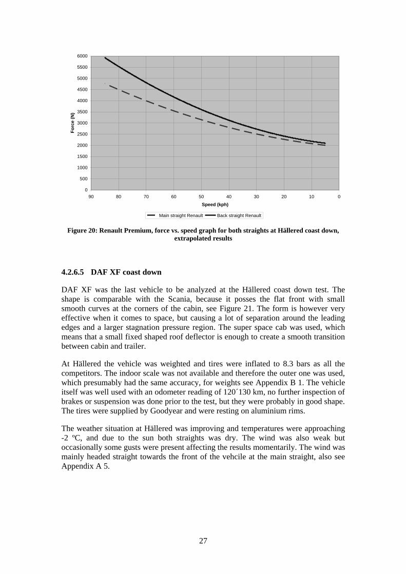
A new road load profile was proposed by using only the vehicle speeds below 50
km/h and then extrapolating the forces up to 85 km/h. Relevant loads should be found
at those speeds, and as long as there is a good relation for the 2nd
order polynomial the
extrapolation should be fairly accurate. The extrapolated load at 85 km/h was
correlated to the theoretical force acting on the vehicle with the particular
specifications, see Equation 1.
NmgfvACF rD 48310052.0*81.9*396306.3
85*82.0*7.9*268.1*5.0
2
12
2
Equation 1
The constants are obtained from the vehicle, the mass is the measured weight, and the
coefficient of rolling resistance is calculated from the force at 5 km/h (assuming no
aerodynamic resistance). The frontal area is approximated from the trailer width 2.55
m times the trailer height of 4 m and finally by subtracting 0.5 m2. The drag
coefficient is obtained from tabulated values of trucks with the specific gap and height
distance between the tractor and trailer. The theoretical force value is a bit lower than
the extrapolated force at 85 km/h in Figure 20, but the formula neglects side winds
and speed depending rolling resistance and therefore a more realistic force would
probably be around 500 N higher and then in between the two straights’ force shown
in Figure 20.
The large differences between the two curves are due to the extrapolation and side
winds that were directed perpendicular to the truck during that day of testing. The
calculated value is however suggesting a similar result as the extrapolation proving
that the forces are at the right magnitude.
27
0
500
1000
1500
2000
2500
3000
3500
4000
4500
5000
5500
6000
0102030405060708090
Speed (kph)
Fo
rce
(N
)
Main straight Renault Back straight Renault
Figure 20: Renault Premium, force vs. speed graph for both straights at Hällered coast down,
extrapolated results
4.2.6.5 DAF XF coast down
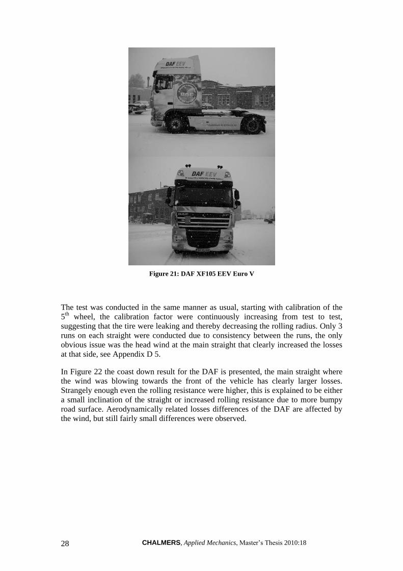
DAF XF was the last vehicle to be analyzed at the Hällered coast down test. The
shape is comparable with the Scania, because it posses the flat front with small
smooth curves at the corners of the cabin, see Figure 21. The form is however very
effective when it comes to space, but causing a lot of separation around the leading
edges and a larger stagnation pressure region. The super space cab was used, which
means that a small fixed shaped roof deflector is enough to create a smooth transition
between cabin and trailer.
At Hällered the vehicle was weighted and tires were inflated to 8.3 bars as all the
competitors. The indoor scale was not available and therefore the outer one was used,
which presumably had the same accuracy, for weights see Appendix B 1. The vehicle
itself was well used with an odometer reading of 120´130 km, no further inspection of
brakes or suspension was done prior to the test, but they were probably in good shape.
The tires were supplied by Goodyear and were resting on aluminium rims.
The weather situation at Hällered was improving and temperatures were approaching
-2 ºC, and due to the sun both straights was dry. The wind was also weak but
occasionally some gusts were present affecting the results momentarily. The wind was
mainly headed straight towards the front of the vehcile at the main straight, also see
Appendix A 5.
CHALMERS, Applied Mechanics, Master’s Thesis 2010:18 28
Figure 21: DAF XF105 EEV Euro V
The test was conducted in the same manner as usual, starting with calibration of the
5th
wheel, the calibration factor were continuously increasing from test to test,
suggesting that the tire were leaking and thereby decreasing the rolling radius. Only 3
runs on each straight were conducted due to consistency between the runs, the only
obvious issue was the head wind at the main straight that clearly increased the losses
at that side, see Appendix D 5.
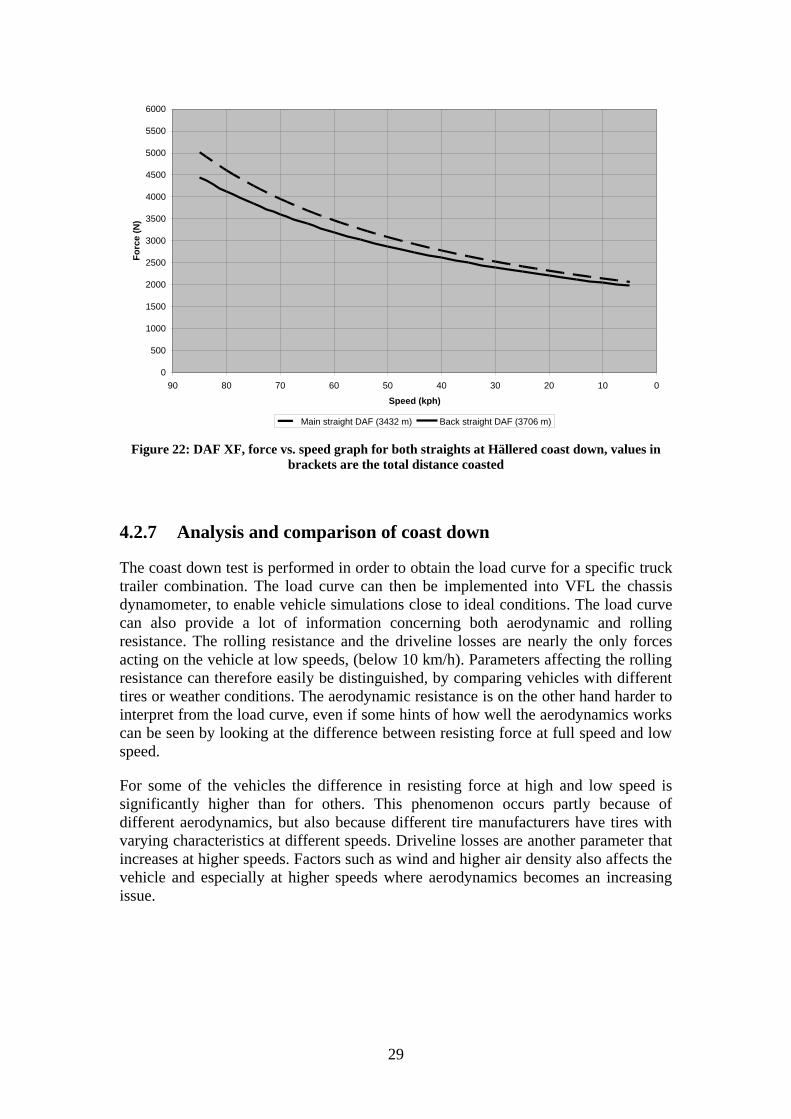
In Figure 22 the coast down result for the DAF is presented, the main straight where
the wind was blowing towards the front of the vehicle has clearly larger losses.
Strangely enough even the rolling resistance were higher, this is explained to be either
a small inclination of the straight or increased rolling resistance due to more bumpy
road surface. Aerodynamically related losses differences of the DAF are affected by
the wind, but still fairly small differences were observed.
29
0
500
1000
1500
2000
2500
3000
3500
4000
4500
5000
5500
6000
0102030405060708090
Speed (kph)
Fo
rce
(N
)
Main straight DAF (3432 m) Back straight DAF (3706 m)
Figure 22: DAF XF, force vs. speed graph for both straights at Hällered coast down, values in
brackets are the total distance coasted
4.2.7 Analysis and comparison of coast down
The coast down test is performed in order to obtain the load curve for a specific truck
trailer combination. The load curve can then be implemented into VFL the chassis
dynamometer, to enable vehicle simulations close to ideal conditions. The load curve
can also provide a lot of information concerning both aerodynamic and rolling
resistance. The rolling resistance and the driveline losses are nearly the only forces
acting on the vehicle at low speeds, (below 10 km/h). Parameters affecting the rolling
resistance can therefore easily be distinguished, by comparing vehicles with different
tires or weather conditions. The aerodynamic resistance is on the other hand harder to
interpret from the load curve, even if some hints of how well the aerodynamics works
can be seen by looking at the difference between resisting force at full speed and low
speed.
For some of the vehicles the difference in resisting force at high and low speed is
significantly higher than for others. This phenomenon occurs partly because of
different aerodynamics, but also because different tire manufacturers have tires with
varying characteristics at different speeds. Driveline losses are another parameter that
increases at higher speeds. Factors such as wind and higher air density also affects the
vehicle and especially at higher speeds where aerodynamics becomes an increasing
issue.
CHALMERS, Applied Mechanics, Master’s Thesis 2010:18 30
4.2.7.1 Aerodynamic comparison
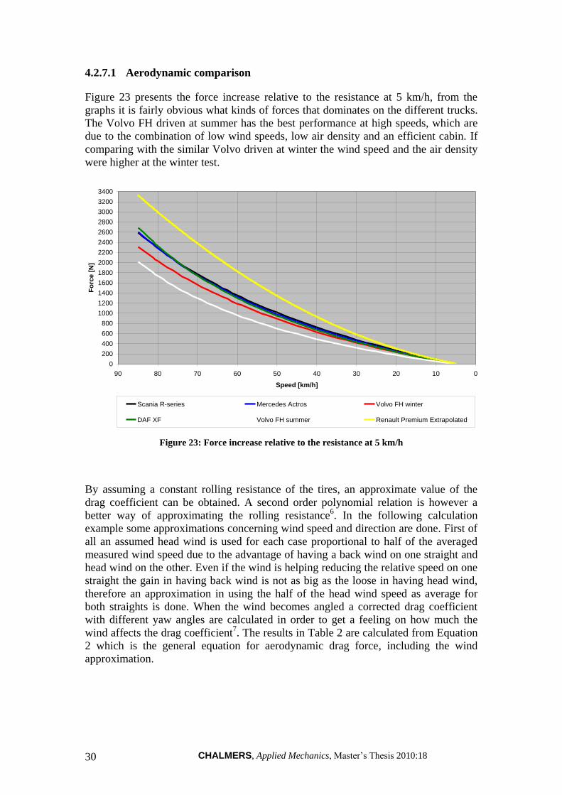
Figure 23 presents the force increase relative to the resistance at 5 km/h, from the
graphs it is fairly obvious what kinds of forces that dominates on the different trucks.
The Volvo FH driven at summer has the best performance at high speeds, which are
due to the combination of low wind speeds, low air density and an efficient cabin. If
comparing with the similar Volvo driven at winter the wind speed and the air density
were higher at the winter test.
0
200
400
600
800
1000
1200
1400
1600
1800
2000
2200
2400
2600
2800
3000
3200
3400
0102030405060708090
Speed [km/h]
Fo
rce
[N
]
Scania R-series Mercedes Actros Volvo FH winter
DAF XF Volvo FH summer Renault Premium Extrapolated
Figure 23: Force increase relative to the resistance at 5 km/h
By assuming a constant rolling resistance of the tires, an approximate value of the
drag coefficient can be obtained. A second order polynomial relation is however a
better way of approximating the rolling resistance6. In the following calculation
example some approximations concerning wind speed and direction are done. First of
all an assumed head wind is used for each case proportional to half of the averaged
measured wind speed due to the advantage of having a back wind on one straight and
head wind on the other. Even if the wind is helping reducing the relative speed on one
straight the gain in having back wind is not as big as the loose in having head wind,
therefore an approximation in using the half of the head wind speed as average for
both straights is done. When the wind becomes angled a corrected drag coefficient
with different yaw angles are calculated in order to get a feeling on how much the
wind affects the drag coefficient7. The results in Table 2 are calculated from Equation
2 which is the general equation for aerodynamic drag force, including the wind
approximation.
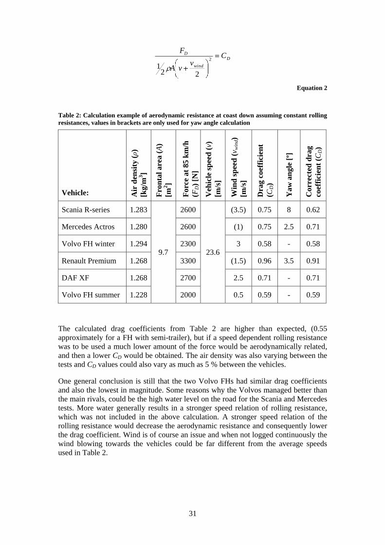
31
D
wind
D Cv
vA
F2
221
Equation 2
Table 2: Calculation example of aerodynamic resistance at coast down assuming constant rolling
resistances, values in brackets are only used for yaw angle calculation
Vehicle: Air
den
sity
(ρ)
[kg/m
3]
Fro
nta
l are
a (
A)
[m2]
Forc
e at
85 k
m/h
(FD)
[N]
Veh
icle
sp
eed
(v)
[m/s
]
Win
d s
pee
d (
v win
d)
[m/s
]
Dra
g c
oef
fici
ent
(CD)
Yaw
an
gle
[º]
Corr
ecte
d d
rag
coef
fici
ent
(CD)
Scania R-series 1.283
9.7
2600
23.6
(3.5) 0.75 8 0.62
Mercedes Actros 1.280 2600 (1) 0.75 2.5 0.71
Volvo FH winter 1.294 2300 3 0.58 - 0.58
Renault Premium 1.268 3300 (1.5) 0.96 3.5 0.91
DAF XF 1.268 2700 2.5 0.71 - 0.71
Volvo FH summer 1.228 2000 0.5 0.59 - 0.59
The calculated drag coefficients from Table 2 are higher than expected, (0.55
approximately for a FH with semi-trailer), but if a speed dependent rolling resistance
was to be used a much lower amount of the force would be aerodynamically related,
and then a lower CD would be obtained. The air density was also varying between the
tests and CD values could also vary as much as 5 % between the vehicles.
One general conclusion is still that the two Volvo FHs had similar drag coefficients
and also the lowest in magnitude. Some reasons why the Volvos managed better than
the main rivals, could be the high water level on the road for the Scania and Mercedes
tests. More water generally results in a stronger speed relation of rolling resistance,
which was not included in the above calculation. A stronger speed relation of the
rolling resistance would decrease the aerodynamic resistance and consequently lower
the drag coefficient. Wind is of course an issue and when not logged continuously the
wind blowing towards the vehicles could be far different from the average speeds
used in Table 2.
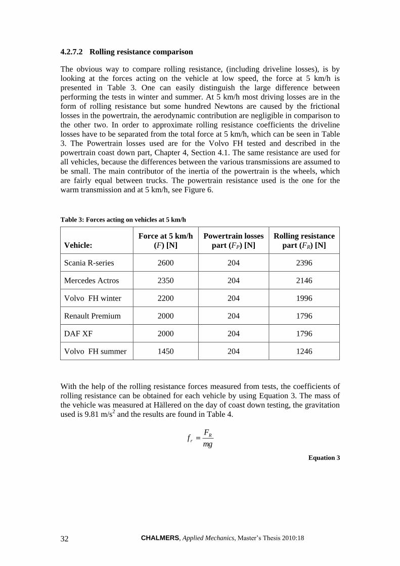
CHALMERS, Applied Mechanics, Master’s Thesis 2010:18 32
4.2.7.2 Rolling resistance comparison
The obvious way to compare rolling resistance, (including driveline losses), is by
looking at the forces acting on the vehicle at low speed, the force at 5 km/h is
presented in Table 3. One can easily distinguish the large difference between
performing the tests in winter and summer. At 5 km/h most driving losses are in the
form of rolling resistance but some hundred Newtons are caused by the frictional
losses in the powertrain, the aerodynamic contribution are negligible in comparison to
the other two. In order to approximate rolling resistance coefficients the driveline
losses have to be separated from the total force at 5 km/h, which can be seen in Table
3. The Powertrain losses used are for the Volvo FH tested and described in the
powertrain coast down part, Chapter 4, Section 4.1. The same resistance are used for
all vehicles, because the differences between the various transmissions are assumed to
be small. The main contributor of the inertia of the powertrain is the wheels, which
are fairly equal between trucks. The powertrain resistance used is the one for the
warm transmission and at 5 km/h, see Figure 6.
Table 3: Forces acting on vehicles at 5 km/h
Vehicle:
Force at 5 km/h
(F) [N]
Powertrain losses
part (FP) [N]
Rolling resistance
part (FR) [N]
Scania R-series 2600 204 2396
Mercedes Actros 2350 204 2146
Volvo FH winter 2200 204 1996
Renault Premium 2000 204 1796
DAF XF 2000 204 1796
Volvo FH summer 1450 204 1246
With the help of the rolling resistance forces measured from tests, the coefficients of
rolling resistance can be obtained for each vehicle by using Equation 3. The mass of
the vehicle was measured at Hällered on the day of coast down testing, the gravitation
used is 9.81 m/s2 and the results are found in Table 4.
mg
Ff R
r
Equation 3
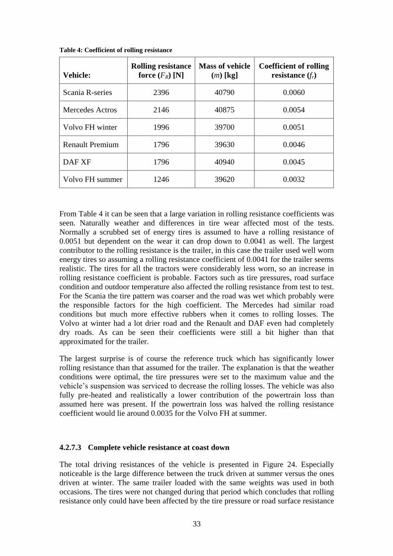
33
Table 4: Coefficient of rolling resistance
Vehicle:
Rolling resistance
force (FR) [N]
Mass of vehicle
(m) [kg]
Coefficient of rolling
resistance (fr)
Scania R-series 2396 40790 0.0060
Mercedes Actros 2146 40875 0.0054
Volvo FH winter 1996 39700 0.0051
Renault Premium 1796 39630 0.0046
DAF XF 1796 40940 0.0045
Volvo FH summer 1246 39620 0.0032
From Table 4 it can be seen that a large variation in rolling resistance coefficients was
seen. Naturally weather and differences in tire wear affected most of the tests.
Normally a scrubbed set of energy tires is assumed to have a rolling resistance of
0.0051 but dependent on the wear it can drop down to 0.0041 as well. The largest
contributor to the rolling resistance is the trailer, in this case the trailer used well worn
energy tires so assuming a rolling resistance coefficient of 0.0041 for the trailer seems
realistic. The tires for all the tractors were considerably less worn, so an increase in
rolling resistance coefficient is probable. Factors such as tire pressures, road surface
condition and outdoor temperature also affected the rolling resistance from test to test.
For the Scania the tire pattern was coarser and the road was wet which probably were
the responsible factors for the high coefficient. The Mercedes had similar road
conditions but much more effective rubbers when it comes to rolling losses. The
Volvo at winter had a lot drier road and the Renault and DAF even had completely
dry roads. As can be seen their coefficients were still a bit higher than that
approximated for the trailer.
The largest surprise is of course the reference truck which has significantly lower
rolling resistance than that assumed for the trailer. The explanation is that the weather
conditions were optimal, the tire pressures were set to the maximum value and the
vehicle’s suspension was serviced to decrease the rolling losses. The vehicle was also
fully pre-heated and realistically a lower contribution of the powertrain loss than
assumed here was present. If the powertrain loss was halved the rolling resistance
coefficient would lie around 0.0035 for the Volvo FH at summer.
4.2.7.3 Complete vehicle resistance at coast down
The total driving resistances of the vehicle is presented in Figure 24. Especially
noticeable is the large difference between the truck driven at summer versus the ones
driven at winter. The same trailer loaded with the same weights was used in both
occasions. The tires were not changed during that period which concludes that rolling
resistance only could have been affected by the tire pressure or road surface resistance
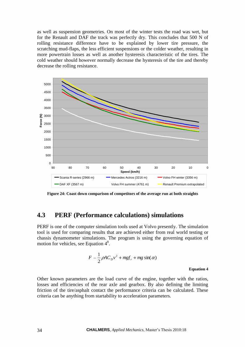
CHALMERS, Applied Mechanics, Master’s Thesis 2010:18 34
as well as suspension geometries. On most of the winter tests the road was wet, but
for the Renault and DAF the track was perfectly dry. This concludes that 500 N of
rolling resistance difference have to be explained by lower tire pressure, the
scratching mud-flaps, the less efficient suspensions or the colder weather, resulting in
more powertrain losses as well as another hysteresis characteristic of the tires. The
cold weather should however normally decrease the hysteresis of the tire and thereby
decrease the rolling resistance.
0
500
1000
1500
2000
2500
3000
3500
4000
4500
5000
0102030405060708090
Speed (km/h)
Fo
rce
(N
)
Scania R-series (2966 m) Mercedes Actros (3216 m) Volvo FH winter (3356 m)
DAF XF (3567 m) Volvo FH summer (4761 m) Renault Premium extrapolated
Figure 24: Coast down comparison of competitors of the average run at both straights
4.3 PERF (Performance calculations) simulations
PERF is one of the computer simulation tools used at Volvo presently. The simulation
tool is used for comparing results that are achieved either from real world testing or
chassis dynamometer simulations. The program is using the governing equation of
motion for vehicles, see Equation 48.
)sin(2
1 2 mgmgfvACF rD
Equation 4
Other known parameters are the load curve of the engine, together with the ratios,
losses and efficiencies of the rear axle and gearbox. By also defining the limiting
friction of the tire/asphalt contact the performance criteria can be calculated. These
criteria can be anything from startability to acceleration parameters.
35
By letting the vehicle drive a predefined route the fuel consumption can be obtained.
There are however a lot of assumption such as the way the vehicle follows the target
speed, the influence of weather e.g. wind, rain and temperature differences. A pre set
wind can be added to the calculation in order to create more realistic drives, but other
climate influences are missing.
4.3.1 Issues with PERF simulations
Even if good approximations of the different driving conditions are used, it is still
difficult to fully simulate the variability of real world driving. For an automated
manual transmission it is however possible to obtain realistic driving scenarios
because the gear shifting degree of freedom is following the same control laws, both
in PERF and in real life driving. The degree of acceleration is however different
between the two types of test, as well as the foreseeing ability a driver possess’. The
main issues are however more related to the difficulty approximating the physical
parameters. The governing equations in PERF are all listed below as Equation 5 -
Equation 9.
e
transfgeng
tracr
iiTF
***
Equation 5
2***
2
1windDD vvCAF
Equation 6
Where:
1000**
*60*2**
fg
eeng
ii
rv
Equation 7
mRF mR *
Equation 8
1000***8.9*01.0 mSFg
Equation 9
S in Equation 9, is the gradient inclination specified in percentage, mathematically
expressed as height travelled divided by length travelled. The mass constant (m) is
here expressed in ton. And as a consequence the rolling resistance coefficient Rm is
based on the mass in ton, the gravitational term is also included in the rolling
coefficient, thereby it has the unit Newton per ton.
CHALMERS, Applied Mechanics, Master’s Thesis 2010:18 36
The tractive effort specified in Equation 5 is also limited to the maximum force the
tires are able to transmit due to coefficient of friction. The friction coefficient is
however simplified as just one value, not dependent on slip, but for most driving cases
the tractive effort never reaches close to the maximum limit. The disadvantages of
describing the drive-cycle with help of above governing equations are the following:
Drag coefficient is the value describing the shapes effectiveness of moving
through air, the value preset in PERF is specific for 80 km/h. For a truck the
shape factor varies with vehicle speed, this effect is however small and is
mostly due to the size of the laminar boundary layer. For a truck where gaps
between the different vehicle parts are big, the boundary layer growth can be
observed at different regions of the truck and consequently affect with a larger
magnitude then for a car for instance. In PERF there is however a sentence in
the results indicating that a certain speed dependence is used, but no relation
of this kind is shown or predefined.
A wind speed can be set in order to simulate more realistic behaviour, the
issue is still that winds are never constant in the real world and can also blow
from behind the truck. The probably most critical wind is also side winds
where a yaw angle towards the truck is created. Such effect changes the drag
coefficient significantly, partly because of more interference around the trailer
gap but also because the heading direction relative to the wind is not parallel
to the length of the truck anymore. The shape of the truck is as a result
changed and so is the effective frontal area.
Air density can easily change the drag force with around 5 % between summer
and winter due to the increased viscosity in cold air. The main factors
affecting the air density is temperature, pressure and humidity. In PERF a
fixed value resembling normal density is used for all simulations.
The effective rolling radius is not constant for all speeds as defined in PERF,
because the centripetal force increases the active wheel radius at high speeds.
Tire rolling resistance coefficient is speed dependent in a second order
polynomial manner while a linear relation is approximating the dependency in
PERF. Rolling resistance coefficient is also much dependent on the type of
asphalt, tire properties, the amount of wear and the smoothness of the road. A
typical constant initial value is used, because all these dependencies are very
difficult to quantify. A lot of information is consequently lost, one example is
up to 20 % difference in rolling resistance coefficient between new and well
worn tires. Other parameters also affecting the rolling resistance coefficient
are tire pressure, temperature of the rubber as well as the temperature of the
inflating air. Finally parameters of the suspension are affecting the easiness of
wheel rotation. Toe-in is one of them and is adjusted positively in order to
create a stable vehicle, but the less toe-in that is used the lower the rolling
resistance coefficient. Brake drag can also be a problem on vehicles even if
trucks usually are not affected due to the pneumatic control of the brake pads.
All these parameters are usually similar between trucks and well recreated in
PERF, but especially when it comes to competitors it is difficult to
approximate the effect of every single component. Consequently a large
uncertainty of the actual rolling resistance is present.
37
Vehicle mass can also vary during tests especially at long cycles where the
amount of fuel can affect the weight with up to 2 % between full and empty
fuel tanks of a 40 ton vehicle. An average mass of the cycle is suitable to use.
When simulating distribution cycles and correlating them to customers’
values, in practice the cargo weight is decreasing and as a result the fuel
consumption drops at the end of the delivery. This is still not a big issue now
that PERF simulations normally are compared to test cycles, and no loading or
unloading is taking place there either.
A significant amount of energy can also be lost by uneven roads resulting in
suspension travel and energy consumed as heat in shock absorbers and
springs.
The transmission efficiency is affected by the amount of oil in the gearbox and
final drive, the gears are usually allowed to splash into the oil in order to
lubricate the contact surface, but some gearboxes are filled with more oil than
others. The efficiencies are preset values representing the friction losses
caused by the contact between gears, this loss is not constant but rather speed
dependent, even if a good approximation can be obtained for the constant. The
efficiency is also strongly dependent on oil viscosity and consequently
temperature of the surrounding air. The temperature relation is unfortunately
difficult to represent because it affects a lot of parameters and a lot of data
would have been required to be stored in the program. Using fully warmed-up
vehicles before the road test is also required in order to be able to correlate the
road test results with PERF, as can be seen from the results achieved in the
powertrain coast down part, Chapter 4, section 4.1.
The engine maps of the particular engines are accessible in PERF but in order
to decrease the amount of data there is only a limited number of torque (Teng)
and engine speed (ωeng) combinations with the definite brake specific fuel
consumption. All other loads and speeds are interpolated between the known
data and as a result is not representing exactly the true value.
When producing an engine map a predefined environment is used, by
comparing this lab environment with the varying climate of a real world test
the engine load can vary a lot, especially if air pressure is changed, for
example at elevated locations.
When simulating in PERF a fixed auxiliary loss is used, based on the normal
requirements. The importance of having similar conditions at the real world
test becomes large, auxiliaries such as the AC compressor can be turned off,
but most others are driven when needed at road tests. Once again outdoor
temperature is affecting, for instance the amount in which the cooling fan is
required. A large increase in power is a result of having the cooling fan
switched on instead of off.
PERF simulations are based on ideal driving conditions, which include no
steering effort. The absence of any resistance caused by steering, such as
increase drag coefficient and increased rolling resistance, results in lower
simulated fuel consumption.
CHALMERS, Applied Mechanics, Master’s Thesis 2010:18 38
A final problem with simulation tools in general is of course the difficulty in
recreating the driver’s contribution, which is not only a problem for simulation
programs, rather a major problem for all tests especially because humans are
unpredictable and some variations can be seen from driver to driver or just test
to test with the same driver.
4.3.2 PERF simulation results
To get some results to analyze, different types of vehicles are simulated with different
technical configurations on two duty cycles. One duty cycle is Lv-Bo-Lv (Landvetter-
Borås-Landvetter), which represents a typical drive for a long-haulage truck, see
Appendix I 1. A target speed for the cycle is also used, for Lv-Bo-Lv that is
constantly 85 km/h, the actual speed is however varying with road inclination and
therefore requires extra accelerations and decelerations to keep the speed, also see
Appendix I 2.
The other duty cycle used is a regional distribution (RDH) cycle which runs on hilly
roads, the reason is to illustrate a contrast to Lv-Bo-Lv and find advantages or
disadvantages of components on different routes. The vehicles simulated can be found
in Appendix J, the different specifications of the vehicle at the duty cycles are also
presented. The technical differences between the simulated vehicles try to illustrate
the areas where improvements can be achieved now and in a near future. The trucks
and their fuel consumption are shown in Table 5.
The largest resistance on a truck is the rolling resistance, by utilizing very low
resistance tires, for instance well worn tires, the fuel consumption can be altered very
much for both drive cycles. The other factor influencing the rolling resistance is the
vehicle mass. For some heavily loaded trucks the weight can not really be decreased,
because a decrease in vehicle weight will only result in more freight. For most trucks
the weight is not limiting but rather the trailer volume and a decrease of mass of the
truck will be a decrease of the total weight. Nevertheless a clear advantage of either
lower fuel consumption or more cargo loading can be obtained by the driver. The
mass of the vehicle is also a factor influencing more at hilly and distribution like
routes where acceleration becomes more important.
The next large influencer is the aerodynamic resistance, which for a truck is less
dominant than the rolling resistance. At Lv-Bo-Lv cycle it becomes more important
than at RDH but still not in the same magnitude as the rolling resistance. The
aerodynamic shape as well as the size, (in this case the frontal area of the trailer),
matters in the same extent to lower the fuel consumption. Frontal area is however
difficult to decrease because loading volume is affected which usually is: the limiting
factor for the transportation. It can also be said here, that a larger difference in fuel
consumption would be achieved if the roof deflector were adjusted poorly and the
trailer height was modified. But in the simulation the same drag coefficient is
assumed. But if relating to the difference between the AA and T052 trailer in the coast
down a much larger would be achieved.
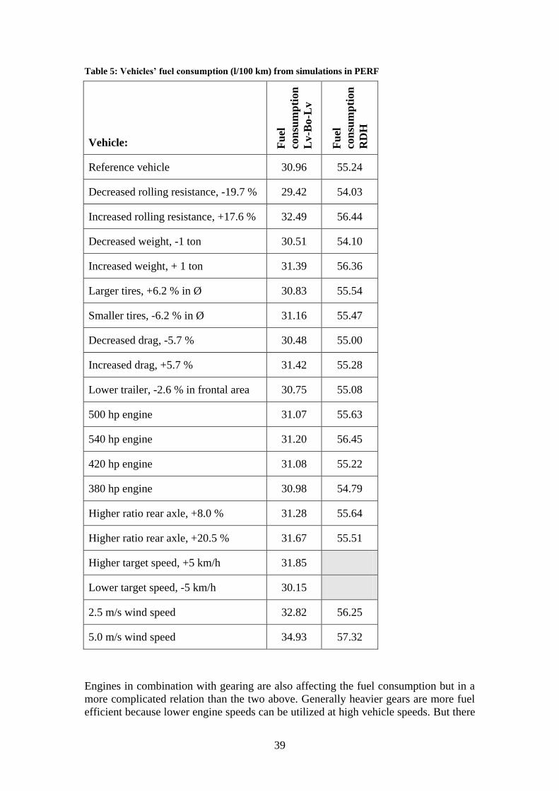
39
Table 5: Vehicles’ fuel consumption (l/100 km) from simulations in PERF
Vehicle: Fu
el
con
sum
pti
on
Lv-B
o-L
v
Fu
el
con
sum
pti
on
RD
H
Reference vehicle 30.96 55.24
Decreased rolling resistance, -19.7 % 29.42 54.03
Increased rolling resistance, +17.6 % 32.49 56.44
Decreased weight, -1 ton 30.51 54.10
Increased weight, + 1 ton 31.39 56.36
Larger tires, +6.2 % in Ø 30.83 55.54
Smaller tires, -6.2 % in Ø 31.16 55.47
Decreased drag, -5.7 % 30.48 55.00
Increased drag, +5.7 % 31.42 55.28
Lower trailer, -2.6 % in frontal area 30.75 55.08
500 hp engine 31.07 55.63
540 hp engine 31.20 56.45
420 hp engine 31.08 55.22
380 hp engine 30.98 54.79
Higher ratio rear axle, +8.0 % 31.28 55.64
Higher ratio rear axle, +20.5 % 31.67 55.51
Higher target speed, +5 km/h 31.85
Lower target speed, -5 km/h 30.15
2.5 m/s wind speed 32.82 56.25
5.0 m/s wind speed 34.93 57.32
Engines in combination with gearing are also affecting the fuel consumption but in a
more complicated relation than the two above. Generally heavier gears are more fuel
efficient because lower engine speeds can be utilized at high vehicle speeds. But there
CHALMERS, Applied Mechanics, Master’s Thesis 2010:18 40
is a limit when low engine speeds tends to increase fuel consumption, if the engine
speed drops to far away from the maximum engine efficiency the fuel consumption
will increase. By decreasing the gear ratios the maximum acceleration and pulling
capability decreases which can be other factors influencing the choice of ratio. It
should also be mentioned that dependent on the duty cycle and the type of driving
different gearing can affect the average operating point of the engine load map, and
thereby change the fuel consumption. By downsizing the engines, in general lower
fuel consumption is obtained, but this is much dependent on the losses of the vehicle.
Lets say that a lot of cargo or an inefficiently equipped tractor is used the engine
might have to be strong in order to run at the optimal operating point at normal
driving, while a smaller engine which consumes less fuel for a certain engine speed
and load needs to run at higher load, in order to produce the same power, and as a
consequence differ from the best efficiency region. Therefore it is difficult to
generalize between which gearing and/or engine that is the most efficient for the
usage and duty cycle.
Lastly some driving conditions are simulated as well, this is done by varying the
target speed from 80 km/h up to 90 km/h for the Lv-Bo-Lv duty cycle. Another
parameter affecting a specific drive is the wind speed. Some experimentation of up to
5 m/s wind speed is conducted in order to describe how much unchangeable wind
conditions can affect the results. The constant head wind of 5 m/s proved to be the
largest single fuel consumption increaser, as can be seen from Table 5. But it should
be kept in mind that it hardly ever blows with a constant headwind of 5 m/s.
4.3.3 Efficient combination in PERF
Some areas of improvement give even higher gains when combining them with others
therefore some simulations of an optimized truck were carried out, Table 6. The most
evident conclusion is that the downsized engine will not contribute to any fuel
consumption gains on the Lv-Bo-Lv cycle and with a gross weight of 40 ton. On the
more energy consuming distribution cycle the less powerful engine performed better,
probably because it operated at higher efficiency regions for longer time than the
more powerful engine. In practice such low fuel consumption obtained from the
optimized vehicles are hard to realize. That is of course as long as the mass is
unchanged. Lower mass can decrease the fuel consumption to a very large extent, as
seen in Table 5, especially if the duty cycle is more of a distribution kind, with a lot of
acceleration. The discussion is however a bit irrelevant because if less cargo is carried
the fuel consumption of the specific truck is decreased, but in such case more vehicles
might be required to move the freight. Two half full trucks are significantly less
effective than one full, but usually it is the volume that limits the amount of freight. A
half full truck on the Lv-Bo-Lv cycle would manage 26.61 l/100 km, with otherwise
the same specifications as the reference vehicle according to simulations.
Downsized engines are discussed frequently in order to decrease future trucks fuel
consumption, from the test the downsizing did not pay off. Partly because the engine
did not decrease in size, (the most obvious difference was the increased turbo
pressure), but it is also dependent on where at the engine load map the operating point
is moved to. From Appendix J it was seen that the average engine torque and power
decreased for the smaller engine during the Lv-Bo-Lv cycle, which suggests that the
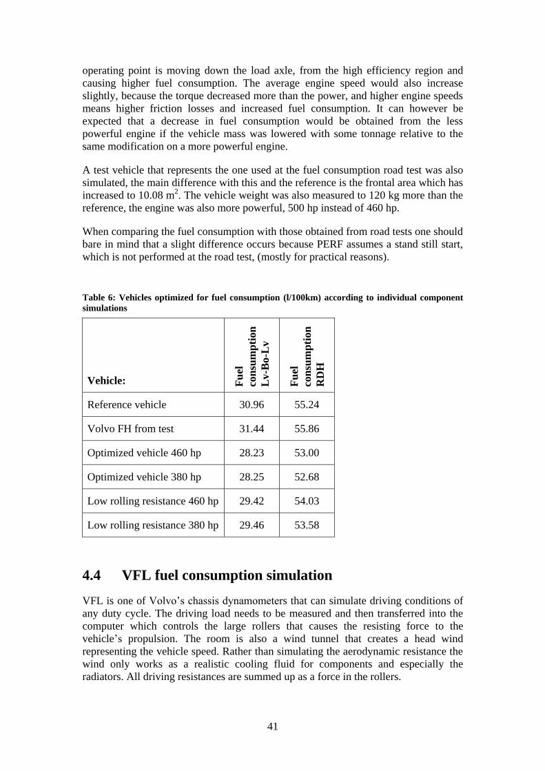
41
operating point is moving down the load axle, from the high efficiency region and
causing higher fuel consumption. The average engine speed would also increase
slightly, because the torque decreased more than the power, and higher engine speeds
means higher friction losses and increased fuel consumption. It can however be
expected that a decrease in fuel consumption would be obtained from the less
powerful engine if the vehicle mass was lowered with some tonnage relative to the
same modification on a more powerful engine.
A test vehicle that represents the one used at the fuel consumption road test was also
simulated, the main difference with this and the reference is the frontal area which has
increased to 10.08 m2. The vehicle weight was also measured to 120 kg more than the
reference, the engine was also more powerful, 500 hp instead of 460 hp.
When comparing the fuel consumption with those obtained from road tests one should
bare in mind that a slight difference occurs because PERF assumes a stand still start,
which is not performed at the road test, (mostly for practical reasons).
Table 6: Vehicles optimized for fuel consumption (l/100km) according to individual component
simulations
Vehicle: Fu
el
con
sum
pti
on
Lv-B
o-L
v
Fu
el
con
sum
pti
on
RD
H
Reference vehicle 30.96 55.24
Volvo FH from test 31.44 55.86
Optimized vehicle 460 hp 28.23 53.00
Optimized vehicle 380 hp 28.25 52.68
Low rolling resistance 460 hp 29.42 54.03
Low rolling resistance 380 hp 29.46 53.58
4.4 VFL fuel consumption simulation
VFL is one of Volvo’s chassis dynamometers that can simulate driving conditions of
any duty cycle. The driving load needs to be measured and then transferred into the
computer which controls the large rollers that causes the resisting force to the
vehicle’s propulsion. The room is also a wind tunnel that creates a head wind
representing the vehicle speed. Rather than simulating the aerodynamic resistance the
wind only works as a realistic cooling fluid for components and especially the
radiators. All driving resistances are summed up as a force in the rollers.
CHALMERS, Applied Mechanics, Master’s Thesis 2010:18 42
The vehicles tested in VFL are the same as the ones used for the coast down, except
for the Volvo, which was with similar specifications but with another wear
characteristic.
4.4.1 Issues with VFL fuel consumption measurement
VFL simulations can only be carried out if an input curve of how the forces on the
vehicle are varying with speed is inserted. That is the main purpose of doing a coast
down test. By using the coast down results all faults that might have occurred during
that test is transferred along with its uncertainties to the VFL test. If it is assumed that
the coast down test is differing by 10 % to the true coast down curve, (that is
approximately a variation of 200 N at low speeds and 300-400 N at top speed), then a
fuel consumption difference of approximately 2-3 % is the outcome. Beside this there
are other factors affecting the results in VFL:
The first thing is the difficulty in approximating a flat road with a roller, the
tire deformation and contact patch is completely changed. There have been
measures taken to compensate for this so probably this issue is small. Then it
should also be remembered that a rubber tire does not have the same friction
limits on a steel roller, and higher slip values can occur, which has to be
compensated for, either by increasing the pull down force, but then less
realistic tire deformation is created, so normally a typical loss caused by this
phenomena is added to the rolling force.
The fuel consumption is measured with two means, either by measuring the
carbon dioxide content in the exhausts and then do chemical carbon balances
in order find the amount of fuel being injected, (the intake air is also needed
to be measured). It is based upon the assumption that all Diesel are being
burnt. In practice some unburned hydrocarbons are passing the engine to the
exhaust. These hydrocarbons are usually fuel that conceal in crevice
volumes such as between the piston and cylinder surface, (that is usually a
very small amount on Diesel engines), some Diesel fuel are present in the
injector sac volume and do not burn due to the rich mixture, the same can
occur in some regions of the combustion chamber where the mixture is to
rich to burn. The carbon balance is also much dependent on an accurate
measurement of the air flow into the engine. Leaks that can occur at every
seal are a very problematic matter, which arises at duty cycles with a lot of
stop and goes. The reason was the sudden increase in intake pressure caused
by the turbo lag when the accelerator pedal is released.
The other way of measuring fuel consumption is by constantly weigh the
amount of fuel supplied to the engine, (any leaks can ruin the results), and
the accuracy of the scale is of course of great importance. The fuel that is
being returned to the fuel tank is also weighted and subtracted from the fuel
feed.
43
When performing a coast down test the combined resistances of rolling,
aerodynamics and driveline are measured. That correlates to the force the
engine is required to overcome in order to propel the vehicle. In VFL that
force can not directly be converted to the rollers, partly because the rollers
own resistance already mentioned. Due to this the force at the rollers has to
be decreased to simulate the reality, but the dragging force on the rollers
should not include the driveline resistance either. The driveline is already
compensated for between the tire and engine and therefore has to be
subtracted from the force curve added to the rollers. That is partly done by
performing a coast down inside VFL, and erasing the difference between the
two coast downs. That difference is the combination of the losses in the
rollers, the driveline and naturally all other factors differing from the real
world coast down test and the one in VFL, such as temperature, weather and
the absence of a trailer. The difference of temperatures in the driveline
between the two tests is also a factor affecting the resistance as was seen in
Chapter 4, Section 4.1.4.
When the total vehicle resistance in VFL is established it needs to match the
coast down profile. The parameters describing the profile are inserted to the
computers and a coast down in VFL is performed with these forces on the
rollers. The final curve is however not usually matching the coast down load
curve and therefore the input parameters needs to be changed by iteration.
By just changing the parameters in order to find a curve matching the coast
down, potential errors can be included and perhaps more importantly: the
individual areas of losses can not be noticeable.
No trailer is used in VFL which means that less work is required from the air
pump for the suspensions. This pump consumes around 6.5 kW when used
and 1 kW when no pumping effort is done, but without the trailer the pump
is used less frequently. So some fuel can be saved by not having the trailer
suspension to feed. On the Lv-Bo-Lv drive cycle around 0.4 % of the fuel
consumption is consumed by the air compressor.9
Lower fuel consumption is achieved in VFL because no increased rolling
resistance due to cornering is assumed, at the same time the power steering
pump is not used and therefore a decrease in fuel consumption of 0.15 % is
obtained for the Lv-Bo-Lv duty cycle.10
Steering not only influences the rolling resistance but an increase in the drag
coefficient, due to a less smooth flow over the trailer gap. The absence of
any steering in the road load and the simulations makes the fuel consumption
somewhat lower than in practice.
4.4.2 VFL drive cycles
Three different drive cycles are simulated in VFL, partly to match the fuel
consumption test cycle but also to get clear correlation for the emissions tests. Lv-Bo-
Lv is the fuel consumption test cycle while Via-Bol-Via, (Viared-Bollebygd-Viared)
and City Hällered are mainly used for emissions. Lv-Bo-Lv was already described in
CHALMERS, Applied Mechanics, Master’s Thesis 2010:18 44
the PERF chapter and is the cycle of highest interest for the fuel consumption part.
Via-Bol-Via test cycle is a new cycle that is mainly intended for emissions, the cycle
is made for two laps of running, in order to get higher confidence of the actual
emission reading.
In order to construct a new test cycle the road needs to be measured with an accurate
GPS where both distance and elevation is continuously logged. Vehicle target speed is
also required to be set. This was done by using the speed limit signs and inserting
them at the right distance measured. During the cycle three stops were made, all lasted
for five minutes in order to simulate how idling emissions affects the results. The
cycle is 73 kilometres and the specific road elevation and target speed can be seen in
Appendix L.
The third cycle is a buss cycle with 12 stops at Hällered’s country side course, which
roughly represents the stopping sequence of a city bus. The cycle is definitely not
representing any common truck drive, but it gives high values of emissions and
thereby more distinguishable results.
4.4.3 VFL fuel consumptions
In VFL the vehicles needs to be carefully prepared with logging equipment of the
vehicle’s ECU parameters. The intake air as well as the exhaust has to be carefully
measured and therefore no leakage in any of the sealing’s are allowed. The air and
exhaust are feed to and from the engine in large pipes that has to be well sealed, the
same applies for the fuel, that is distributed from an external fuel tank in order to
measure the amounts. The vehicle is held in place on the rollers by a steel
construction that forces the rear wheels down with the certain drive axle load,
previously measured.
The front wheels are also connected to a set of rollers. These rollers does not create
any resistance, but are mainly intended to rotate the front wheels with the same speed
as the rear in order to have a correctly measured vehicle speed that is needed for some
of the electrical control systems in the vehicle.
The vehicles were also equipped with PEMS (Portable Emissions Measurement
System) equipment, to measure emissions in the proposed legislative way. The PEMS
is basically an exhaust analyzer that correlates the exhaust with a reference tube filled
with the pure emission composition. More extensive information about the PEMS
equipment is not fitting inside the boundaries of this text.
The fuel consumption is measured in two different ways as described earlier, the
results of the two methods are shown in Table 7, Table 9 and Table 10 for the
different duty cycles respectively. Generally the weighting is the more accurate one,
as long as no leaks are present, the fuel parameters of the Diesel fuel is shown in
Appendix M 1. The tests were conducted at two different operating temperatures, 10
and 25 ºC in order to get a feeling in how the emissions were affected by lower
temperatures. But even the fuel consumption is temperature dependent.
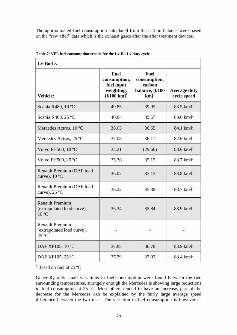
45
The approximated fuel consumption calculated from the carbon balance were based
on the “raw after” data which is the exhaust gases after the after treatment devices.
Table 7: VFL fuel consumption results for the Lv-Bo-Lv duty cycle
Lv-Bo-Lv
Vehicle:
Fuel
consumption,
fuel input
weighting,
[l/100 km]1
Fuel
consumption,
carbon
balance, [l/100
km]1
Average duty
cycle speed
Scania R480, 10 ºC 40.85 39.05 83.5 km/h
Scania R480, 25 ºC 40.84 39.67 83.6 km/h
Mercedes Actros, 10 ºC 38.03 36.65 84.1 km/h
Mercedes Actros, 25 ºC 37.08 36.11 82.6 km/h
Volvo FH500, 10 ºC 35.21 (29.66) 83.6 km/h
Volvo FH500, 25 ºC 35.36 35.15 83.7 km/h
Renault Premium (DAF load
curve), 10 ºC 36.02 35.15 83.8 km/h
Renault Premium (DAF load
curve), 25 ºC 36.22 35.38 83.7 km/h
Renault Premium
(extrapolated load curve),
10 ºC
36.34 35.84 83.9 km/h
Renault Premium
(extrapolated load curve),
25 ºC
- - -
DAF XF105, 10 ºC 37.85 36.78 83.9 km/h
DAF XF105, 25 ºC 37.79 37.02 83.4 km/h
1 Based on fuel at 25 ºC
Generally only small variations in fuel consumption were found between the two
surrounding temperatures, strangely enough the Mercedes is showing large reductions
in fuel consumption at 25 ºC. Most others tended to have an increase, part of the
decrease for the Mercedes can be explained by the fairly large average speed
difference between the two tests. The variation in fuel consumption is however as
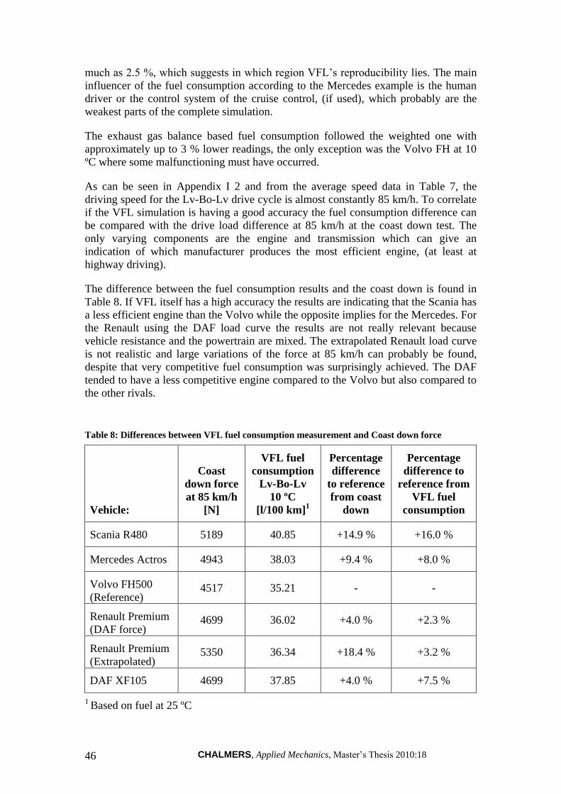
CHALMERS, Applied Mechanics, Master’s Thesis 2010:18 46
much as 2.5 %, which suggests in which region VFL’s reproducibility lies. The main
influencer of the fuel consumption according to the Mercedes example is the human
driver or the control system of the cruise control, (if used), which probably are the
weakest parts of the complete simulation.
The exhaust gas balance based fuel consumption followed the weighted one with
approximately up to 3 % lower readings, the only exception was the Volvo FH at 10
ºC where some malfunctioning must have occurred.
As can be seen in Appendix I 2 and from the average speed data in Table 7, the
driving speed for the Lv-Bo-Lv drive cycle is almost constantly 85 km/h. To correlate
if the VFL simulation is having a good accuracy the fuel consumption difference can
be compared with the drive load difference at 85 km/h at the coast down test. The
only varying components are the engine and transmission which can give an
indication of which manufacturer produces the most efficient engine, (at least at
highway driving).
The difference between the fuel consumption results and the coast down is found in
Table 8. If VFL itself has a high accuracy the results are indicating that the Scania has
a less efficient engine than the Volvo while the opposite implies for the Mercedes. For
the Renault using the DAF load curve the results are not really relevant because
vehicle resistance and the powertrain are mixed. The extrapolated Renault load curve
is not realistic and large variations of the force at 85 km/h can probably be found,
despite that very competitive fuel consumption was surprisingly achieved. The DAF
tended to have a less competitive engine compared to the Volvo but also compared to
the other rivals.
Table 8: Differences between VFL fuel consumption measurement and Coast down force
Vehicle:
Coast
down force
at 85 km/h
[N]
VFL fuel
consumption
Lv-Bo-Lv
10 ºC
[l/100 km]1
Percentage
difference
to reference
from coast
down
Percentage
difference to
reference from
VFL fuel
consumption
Scania R480 5189 40.85 +14.9 % +16.0 %
Mercedes Actros 4943 38.03 +9.4 % +8.0 %
Volvo FH500
(Reference) 4517 35.21 - -
Renault Premium
(DAF force) 4699 36.02 +4.0 % +2.3 %
Renault Premium
(Extrapolated) 5350 36.34 +18.4 % +3.2 %
DAF XF105 4699 37.85 +4.0 % +7.5 %
1 Based on fuel at 25 ºC
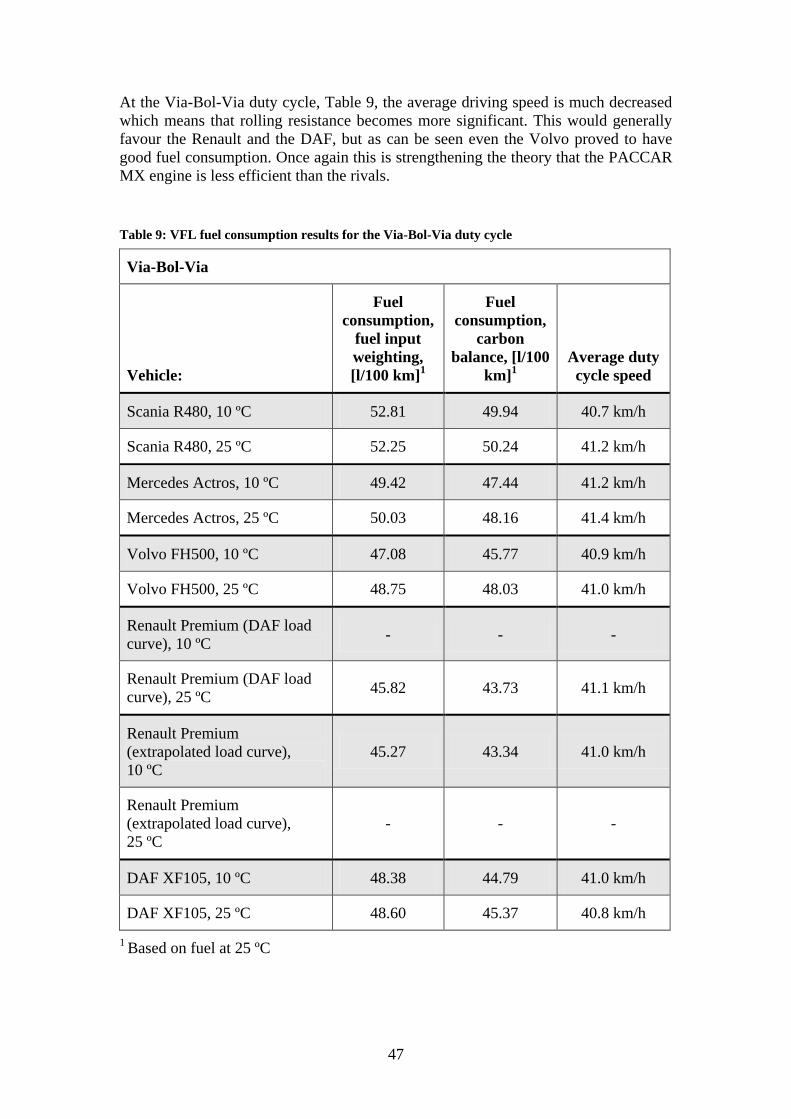
47
At the Via-Bol-Via duty cycle, Table 9, the average driving speed is much decreased
which means that rolling resistance becomes more significant. This would generally
favour the Renault and the DAF, but as can be seen even the Volvo proved to have
good fuel consumption. Once again this is strengthening the theory that the PACCAR
MX engine is less efficient than the rivals.
Table 9: VFL fuel consumption results for the Via-Bol-Via duty cycle
Via-Bol-Via
Vehicle:
Fuel
consumption,
fuel input
weighting,
[l/100 km]1
Fuel
consumption,
carbon
balance, [l/100
km]1
Average duty
cycle speed
Scania R480, 10 ºC 52.81 49.94 40.7 km/h
Scania R480, 25 ºC 52.25 50.24 41.2 km/h
Mercedes Actros, 10 ºC 49.42 47.44 41.2 km/h
Mercedes Actros, 25 ºC 50.03 48.16 41.4 km/h
Volvo FH500, 10 ºC 47.08 45.77 40.9 km/h
Volvo FH500, 25 ºC 48.75 48.03 41.0 km/h
Renault Premium (DAF load
curve), 10 ºC - - -
Renault Premium (DAF load
curve), 25 ºC 45.82 43.73 41.1 km/h
Renault Premium
(extrapolated load curve),
10 ºC
45.27 43.34 41.0 km/h
Renault Premium
(extrapolated load curve),
25 ºC
- - -
DAF XF105, 10 ºC 48.38 44.79 41.0 km/h
DAF XF105, 25 ºC 48.60 45.37 40.8 km/h
1 Based on fuel at 25 ºC
CHALMERS, Applied Mechanics, Master’s Thesis 2010:18 48
The City Hällered bus cycle is driven at even lower average speeds and consequently
an even larger part of the resistances are rolling resistances. At such low speeds and
frequent stop and go’s, large losses due to acceleration and idling occurs, therefore a
fuel efficient engine is vital. According to the test results the Scania is more fuel
efficient than the Mercedes which probably can be described by the long periods of
idling, but also because a large uncertainty can be found in the results, the carbon
balance method for instance describes the opposite.
Large differences between the two temperatures can also be found, few conclusions
can however be drawn because the fuel consumption are higher at 25 ºC for some
trucks and lower for others.
The perhaps most evident conclusion from the bus cycle is that the fuel consumption
is doubled in comparison to the distribution cycle Via-Bol-Via. Hybridization can
therefore be an efficient improvement for the propulsion system at vehicles operating
in city traffic, in general buses.
The two measurement methods did also show a large difference in values, the reason
for this is assumed to be the large variation in intake pressure due to many hard
accelerations and engine braking which can cause high pressure gradients and leakage
at the seals. The extra air that either is drawn in or pushed out destroys the carbon
balance, due to the inaccurate air mass reading. The effect was most evident for the
competitor vehicles, suggesting that the connection between the intake system and the
feed pipe was less suitable, in comparison to the Volvo.
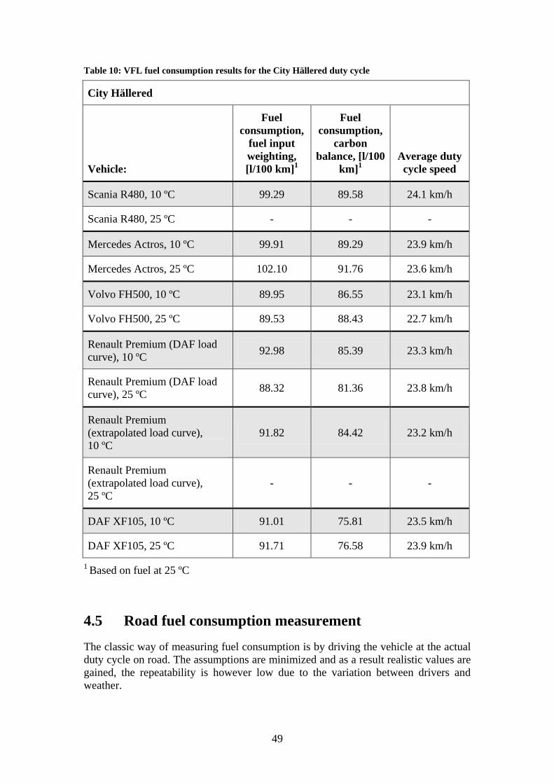
49
Table 10: VFL fuel consumption results for the City Hällered duty cycle
City Hällered
Vehicle:
Fuel
consumption,
fuel input
weighting,
[l/100 km]1
Fuel
consumption,
carbon
balance, [l/100
km]1
Average duty
cycle speed
Scania R480, 10 ºC 99.29 89.58 24.1 km/h
Scania R480, 25 ºC - - -
Mercedes Actros, 10 ºC 99.91 89.29 23.9 km/h
Mercedes Actros, 25 ºC 102.10 91.76 23.6 km/h
Volvo FH500, 10 ºC 89.95 86.55 23.1 km/h
Volvo FH500, 25 ºC 89.53 88.43 22.7 km/h
Renault Premium (DAF load
curve), 10 ºC 92.98 85.39 23.3 km/h
Renault Premium (DAF load
curve), 25 ºC 88.32 81.36 23.8 km/h
Renault Premium
(extrapolated load curve),
10 ºC
91.82 84.42 23.2 km/h
Renault Premium
(extrapolated load curve),
25 ºC
- - -
DAF XF105, 10 ºC 91.01 75.81 23.5 km/h
DAF XF105, 25 ºC 91.71 76.58 23.9 km/h
1 Based on fuel at 25 ºC
4.5 Road fuel consumption measurement
The classic way of measuring fuel consumption is by driving the vehicle at the actual
duty cycle on road. The assumptions are minimized and as a result realistic values are
gained, the repeatability is however low due to the variation between drivers and
weather.
CHALMERS, Applied Mechanics, Master’s Thesis 2010:18 50
The measurement is conducted with help of a portable flow meter that accurately
measures the fuel by measuring the amount of pulses of a constant volume that is feed
by a cog gear. The amount of fuel is manually inserted to a file when a specific
interval of the duty cycle is finished. The truck is also driven along with a reference
truck that is equipped with the same measurement device, the same reference is used
for all the tested trucks.
The road test is performed at the Borås-Landvetter duty cycle, note that for the road
test there is a higher convenience of driving in the opposite direction Bo-Lv-Bo. The
cycle is still the same and no difference in fuel consumption should be witnessed.
After the test the two trucks are normalized in order get comparable fuel
consumptions. Factors such as weight frontal area and average speed are normalizing
the fuel consumption with approximate correction factors, see Section 4.5.2.
4.5.1 Issues with road testing of fuel consumption
Even if road tests gives accurate results there is plenty of issues that can affect the
absolute value between tests and days. The reference truck is however a good
insurance and can make errors or vehicle differences distinguishable.
At the road test two different fuel reference trailers were used and shifted
between the tested vehicle and the reference vehicle, by taking the average
of the different runs a good correlation is achieved. The trailers were
however not the same as the one used at the coast down and which later on
was used as base in VFL. The trailer height was almost the same, (the AA
trailer was five centimetres higher), but other factors such as tire type and
size, as well as aerodynamic components such as trailer side skirts were
different.
Weather can affect the results significantly, especially rain (such weathers
are however avoided) but also temperatures and winds.
One of the most sensitive areas of road testing is the drivers. At this test two
different drivers were used which naturally worsen things because it is
difficult for them to do the same kind of drive when it comes to accelerations
and decelerations.
All vehicle specific components that are found on some of the trucks but not
on others are of course an error that is difficult to omit. This problem is on
the other hand not specific for these kinds of tests. It also depends on what
kind of comparison that is wanted: between competitors or between test
methods. As long as the vehicles are comparable on equal grounds, their
specific components are of less importance.
The measurement equipment is an area of concern because a very accurate
device is needed not get small errors of every sample that is measured, in the
end such inaccuracies can become notable. The accuracy of the fuel flow
measurement device should be within 0.5 %, according to its specification.
51
The tires used on the tractors for the fuel consumption tests were the same
for all runs except for the Mercedes Actros which required smaller diameter
wheels. The tire type and pattern were different and potentially affecting the
Mercedes negatively
If a comparison between the VFL results and the road test results is to be
carried out on equal ground the trailers and tires should be similar at both
occasions. At the road test the tractor tires were shifted to similar ones for all
trucks while the coast down utilized the tires fitted to the tractor initially.
The trailers were also different between the two tests where the coast down
trailer T052 was equipped with side skirts and well worn tires of other
dimensions.
4.5.2 Road test corrections
When conducting the road fuel consumption testing a reference truck is used to
correlate if external influencing factors are affecting the test. The reference is serviced
frequently and thereby repeatable results should be achieved unless weather or driving
behaviour has changed a lot.
The fuel consumption result is also manually transformed for the reference truck in
case there are vehicular variations between the two trucks. The main disadvantage of
correcting the reference truck’s fuel consumption is that it becomes non comparable
to the other tests where the reference vehicle is corrected for another vehicle
configuration. But in case the difference between the reference and the tested vehicle
is wanted the method is the most accurate one. It can still be argued whether it is fair
or not to compensate for weight differences, if a truck is managing to carry the same
load and still be lighter then a competitor, should the fuel consumption really needed
to be increased for compensation?
Five parameters are presently used for normalization: difference in vehicle average
speed, difference in aerodynamic and rolling resistance coefficients (in these tests the
coefficients were not measured and therefore no corrections were done), the vehicle
frontal area and the vehicle weight. The first parameter is the only one that is not
vehicle specific and the most important one to normalize, the correction of the speed
is based on the measured average speed between the start mark and the Ellos sign on
the Bo-Lv-Bo cycle. This part of the duty cycle is flat and can by that distinguish
differences in the control systems of the cruise control. The cruise control is basically
used for the complete cycle, and a difference at the flat part will contribute to a similar
error throughout the cycle.11
The normalization factors are established from PERF simulations of the specific duty
cycle segments, they should be seen more like guidelines rather than absolute values,
the factors can be seen in Table 11. The base values are the ones obtained from the
tested truck, while the correction is done on the reference truck. The absolute value
gained from the reference truck is of less interest while the difference between the two
trucks is important.
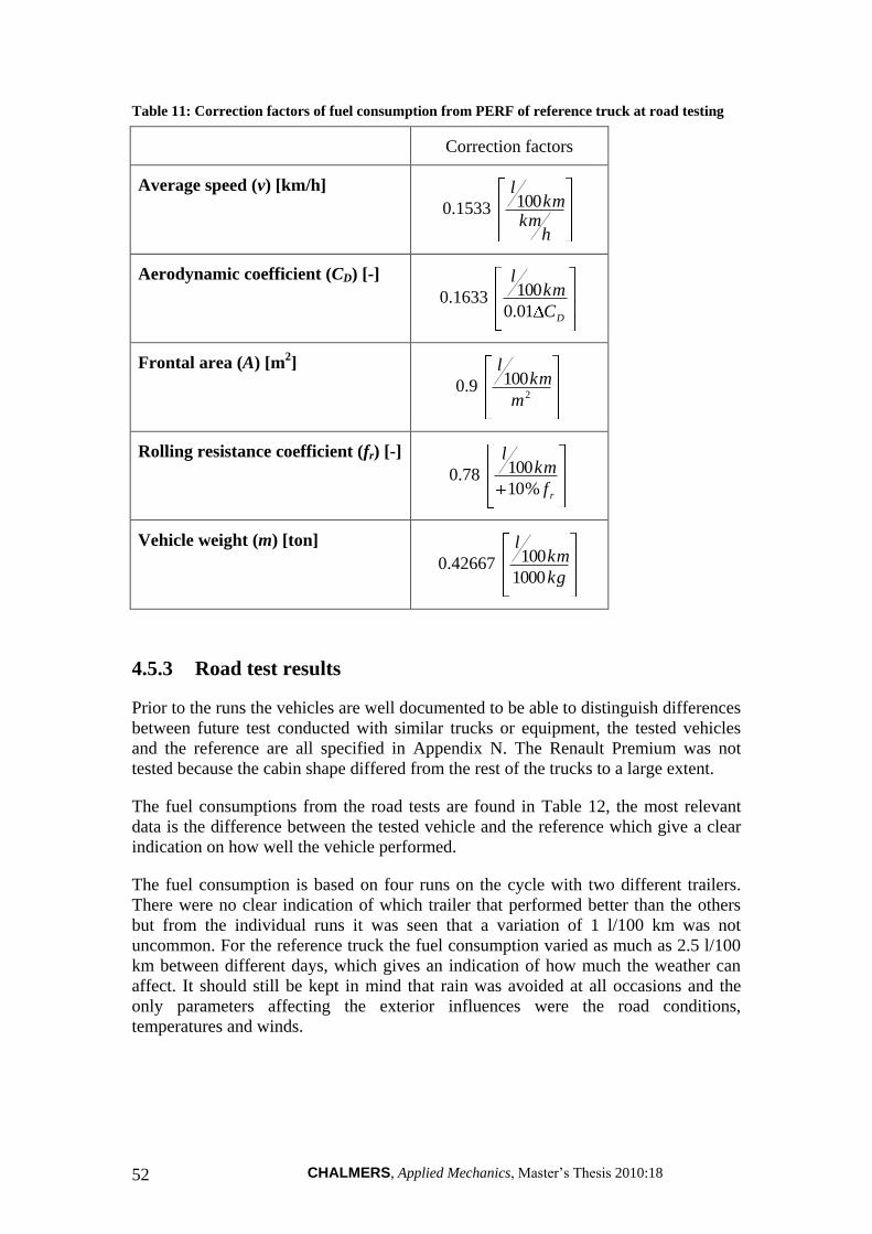
CHALMERS, Applied Mechanics, Master’s Thesis 2010:18 52
Table 11: Correction factors of fuel consumption from PERF of reference truck at road testing
Correction factors
Average speed (v) [km/h]
0.1533
hkm
kml100
Aerodynamic coefficient (CD) [-]
0.1633 DC
kml
01.0
100
Frontal area (A) [m2]
0.9 2
100
m
kml
Rolling resistance coefficient (fr) [-]
0.78 rf
kml
%10
100
Vehicle weight (m) [ton]
0.42667 kg
kml
1000
100
4.5.3 Road test results
Prior to the runs the vehicles are well documented to be able to distinguish differences
between future test conducted with similar trucks or equipment, the tested vehicles
and the reference are all specified in Appendix N. The Renault Premium was not
tested because the cabin shape differed from the rest of the trucks to a large extent.
The fuel consumptions from the road tests are found in Table 12, the most relevant
data is the difference between the tested vehicle and the reference which give a clear
indication on how well the vehicle performed.
The fuel consumption is based on four runs on the cycle with two different trailers.
There were no clear indication of which trailer that performed better than the others
but from the individual runs it was seen that a variation of 1 l/100 km was not
uncommon. For the reference truck the fuel consumption varied as much as 2.5 l/100
km between different days, which gives an indication of how much the weather can
affect. It should still be kept in mind that rain was avoided at all occasions and the
only parameters affecting the exterior influences were the road conditions,
temperatures and winds.
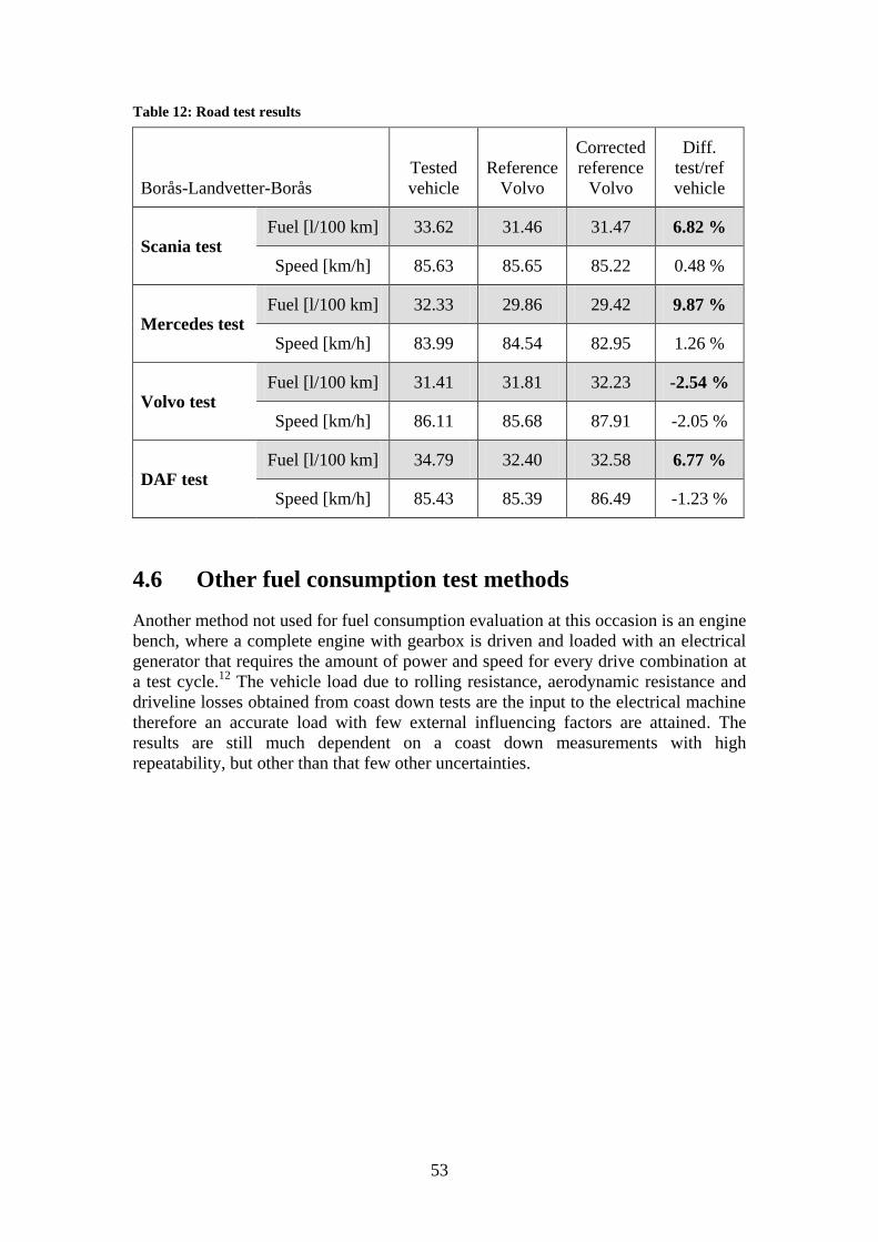
53
Table 12: Road test results
Borås-Landvetter-Borås
Tested
vehicle
Reference
Volvo
Corrected
reference
Volvo
Diff.
test/ref
vehicle
Scania test Fuel [l/100 km] 33.62 31.46 31.47 6.82 %
Speed [km/h] 85.63 85.65 85.22 0.48 %
Mercedes test Fuel [l/100 km] 32.33 29.86 29.42 9.87 %
Speed [km/h] 83.99 84.54 82.95 1.26 %
Volvo test Fuel [l/100 km] 31.41 31.81 32.23 -2.54 %
Speed [km/h] 86.11 85.68 87.91 -2.05 %
DAF test Fuel [l/100 km] 34.79 32.40 32.58 6.77 %
Speed [km/h] 85.43 85.39 86.49 -1.23 %
4.6 Other fuel consumption test methods
Another method not used for fuel consumption evaluation at this occasion is an engine
bench, where a complete engine with gearbox is driven and loaded with an electrical
generator that requires the amount of power and speed for every drive combination at
a test cycle.12
The vehicle load due to rolling resistance, aerodynamic resistance and
driveline losses obtained from coast down tests are the input to the electrical machine
therefore an accurate load with few external influencing factors are attained. The
results are still much dependent on a coast down measurements with high
repeatability, but other than that few other uncertainties.
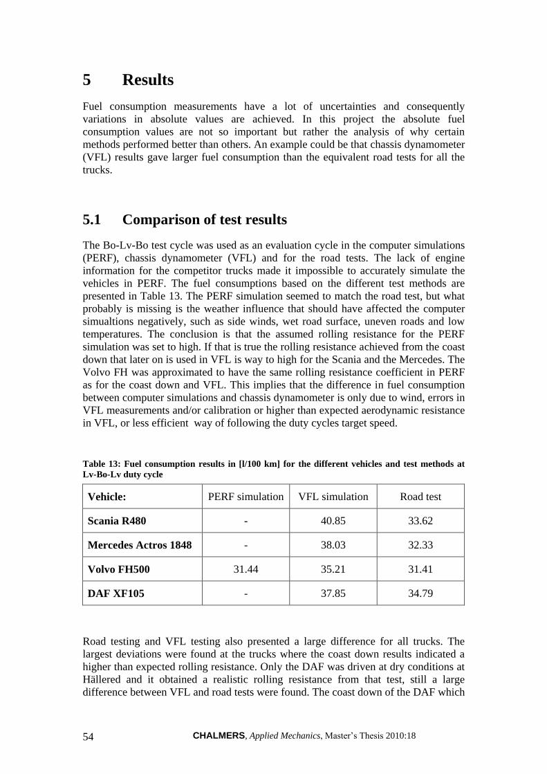
CHALMERS, Applied Mechanics, Master’s Thesis 2010:18 54
5 Results
Fuel consumption measurements have a lot of uncertainties and consequently
variations in absolute values are achieved. In this project the absolute fuel
consumption values are not so important but rather the analysis of why certain
methods performed better than others. An example could be that chassis dynamometer
(VFL) results gave larger fuel consumption than the equivalent road tests for all the
trucks.
5.1 Comparison of test results
The Bo-Lv-Bo test cycle was used as an evaluation cycle in the computer simulations
(PERF), chassis dynamometer (VFL) and for the road tests. The lack of engine
information for the competitor trucks made it impossible to accurately simulate the
vehicles in PERF. The fuel consumptions based on the different test methods are
presented in Table 13. The PERF simulation seemed to match the road test, but what
probably is missing is the weather influence that should have affected the computer
simualtions negatively, such as side winds, wet road surface, uneven roads and low
temperatures. The conclusion is that the assumed rolling resistance for the PERF
simulation was set to high. If that is true the rolling resistance achieved from the coast
down that later on is used in VFL is way to high for the Scania and the Mercedes. The
Volvo FH was approximated to have the same rolling resistance coefficient in PERF
as for the coast down and VFL. This implies that the difference in fuel consumption
between computer simulations and chassis dynamometer is only due to wind, errors in
VFL measurements and/or calibration or higher than expected aerodynamic resistance
in VFL, or less efficient way of following the duty cycles target speed.
Table 13: Fuel consumption results in [l/100 km] for the different vehicles and test methods at
Lv-Bo-Lv duty cycle
Vehicle: PERF simulation VFL simulation Road test
Scania R480 - 40.85 33.62
Mercedes Actros 1848 - 38.03 32.33
Volvo FH500 31.44 35.21 31.41
DAF XF105 - 37.85 34.79
Road testing and VFL testing also presented a large difference for all trucks. The
largest deviations were found at the trucks where the coast down results indicated a
higher than expected rolling resistance. Only the DAF was driven at dry conditions at
Hällered and it obtained a realistic rolling resistance from that test, still a large
difference between VFL and road tests were found. The coast down of the DAF which
55
the VFL results are based upon were conducted at close to ideal conditions with low
wind speeds and head wind in one direction and tail wind in the other. The weather at
the road test can not be assumed to be much better, which concludes that VFL results
generally give higher fuel consumption than road tests.
In the PERF chapter, Table 5 differences between 0.006 and 0.0041 were simulated to
be 3 l/100 km at the Lv-Bo-Lv drive cycle. A rolling resistance coefficient of 0.0041
is far lower than expected for a truck but even with this kind of decrease the Scania’s
VFL fuel consumption would lie around 38 l/100 km, according to PERF simulations
Table 5. Even with this correction the difference between the methods is above 4
l/100 km. From the weather information in Appendix A it is seen that a side wind of
around 3-4 m/s was present at the coast down of the Scania, if it is assumed that this
can be represented by a constant head wind of 2.5 m/s, which probably is an
exaggeration, the fuel consumption would decrease by 2 l/100 km further on the Lv-
Bo-Lv drive cycle. After these corrections a difference between the test methods
similar to that of the DAF is obtained.
According to the examples evaluated previously the VFL results tends to overestimate
the fuel consumption, alternatively the road test is underestimating them. The later
alternative is however less probable because the only parts which can underestimate
the fuel consumption in the measurement are the fuel or the speed measuring devices.
Vehicle failures can of course occur but such issues are usually affecting the results
more evidently. Then it should also be mentioned that the road test correlated well
with the PERF simulation. The PERF simulation should however be lower because it
is ideal, but it was probably affected by a too high estimation of the rolling resistance.
(Estimation based on the coast down result, where slightly wet road was used which
equalled Energy tires in rolling resistance in PERF). For the road tests the rolling
resistance were minimized by using worn Michelin energy tires, which of course
decreased the fuel consumption, but hardly below 0.0041 which was simulated in the
PERF section as a test. But for VFL fuel consumption to decrease to the same
magnitude as for the road tests even lower rolling resistance is needed. Another factor
could be the higher than allowed target speed. At the road tests similar speeds were
used, but the measured value could be measured inaccurately.
The weighting of fuel in VFL is at least as accurate as the measurement at the road
test and therefore no big difference should be found. The difference in fuel
consumption should then lie with the road load adaption or calibration. Road load
curves are not inserted directly to the rollers, because the loss caused by the friction of
the rollers’ bearings, the inertia of the rollers as well as the powertrain must be
excluded from the road load at the wheels. Therefore a similar coast down is
performed in VFL, the resulting graph is adjusted by changing load parameters in
VFL in order to get the shape of the actual coast down curve. The procedure is a trial
and error way of doing things and large uncertainties occurs, especially because the
road load in VFL is to represent a road load performed in another environment.
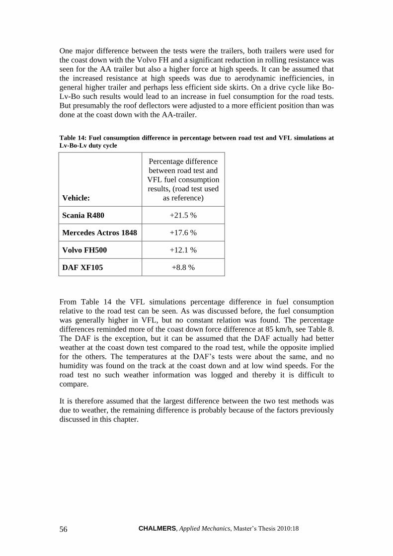
CHALMERS, Applied Mechanics, Master’s Thesis 2010:18 56
One major difference between the tests were the trailers, both trailers were used for
the coast down with the Volvo FH and a significant reduction in rolling resistance was
seen for the AA trailer but also a higher force at high speeds. It can be assumed that
the increased resistance at high speeds was due to aerodynamic inefficiencies, in
general higher trailer and perhaps less efficient side skirts. On a drive cycle like Bo-
Lv-Bo such results would lead to an increase in fuel consumption for the road tests.
But presumably the roof deflectors were adjusted to a more efficient position than was
done at the coast down with the AA-trailer.
Table 14: Fuel consumption difference in percentage between road test and VFL simulations at
Lv-Bo-Lv duty cycle
Vehicle:
Percentage difference
between road test and
VFL fuel consumption
results, (road test used
as reference)
Scania R480 +21.5 %
Mercedes Actros 1848 +17.6 %
Volvo FH500 +12.1 %
DAF XF105 +8.8 %
From Table 14 the VFL simulations percentage difference in fuel consumption
relative to the road test can be seen. As was discussed before, the fuel consumption
was generally higher in VFL, but no constant relation was found. The percentage
differences reminded more of the coast down force difference at 85 km/h, see Table 8.
The DAF is the exception, but it can be assumed that the DAF actually had better
weather at the coast down test compared to the road test, while the opposite implied
for the others. The temperatures at the DAF’s tests were about the same, and no
humidity was found on the track at the coast down and at low wind speeds. For the
road test no such weather information was logged and thereby it is difficult to
compare.
It is therefore assumed that the largest difference between the two test methods was
due to weather, the remaining difference is probably because of the factors previously
discussed in this chapter.
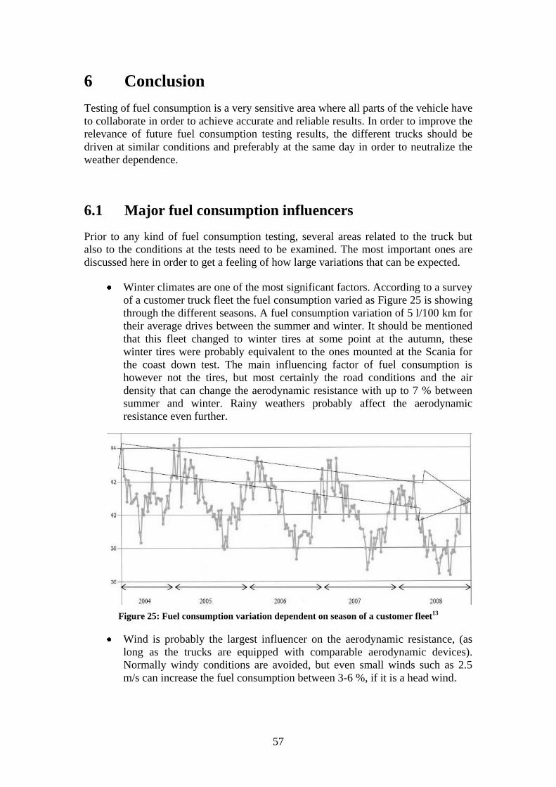
57
6 Conclusion
Testing of fuel consumption is a very sensitive area where all parts of the vehicle have
to collaborate in order to achieve accurate and reliable results. In order to improve the
relevance of future fuel consumption testing results, the different trucks should be
driven at similar conditions and preferably at the same day in order to neutralize the
weather dependence.
6.1 Major fuel consumption influencers
Prior to any kind of fuel consumption testing, several areas related to the truck but
also to the conditions at the tests need to be examined. The most important ones are
discussed here in order to get a feeling of how large variations that can be expected.
Winter climates are one of the most significant factors. According to a survey
of a customer truck fleet the fuel consumption varied as Figure 25 is showing
through the different seasons. A fuel consumption variation of 5 l/100 km for
their average drives between the summer and winter. It should be mentioned
that this fleet changed to winter tires at some point at the autumn, these
winter tires were probably equivalent to the ones mounted at the Scania for
the coast down test. The main influencing factor of fuel consumption is
however not the tires, but most certainly the road conditions and the air
density that can change the aerodynamic resistance with up to 7 % between
summer and winter. Rainy weathers probably affect the aerodynamic
resistance even further.
Figure 25: Fuel consumption variation dependent on season of a customer fleet13
Wind is probably the largest influencer on the aerodynamic resistance, (as
long as the trucks are equipped with comparable aerodynamic devices).
Normally windy conditions are avoided, but even small winds such as 2.5
m/s can increase the fuel consumption between 3-6 %, if it is a head wind.
CHALMERS, Applied Mechanics, Master’s Thesis 2010:18 58
The most significant aerodynamic features should be the same between
trucks to even hope for comparable results. Such devices are mainly the roof
and side deflectors which are critical in order to decrease the aerodynamic
drag coefficient. From VFL it was seen that the Renault Premium still
performed well in fuel consumption, but it should be kept in mind that non-
realistic force curves were used, and that the rolling resistance of the Renault
was even better than the rest of the rivals, (due to dry roads at the coast down
test).
Tires can also vary the rolling resistance largely. Partly because of different
compounds, patterns, dimensions but also because of the wear. Therefore
future testing will require standard sets of tires to be used for all vehicles.
It is important to run-in vehicles before the testing, much increased losses in
bearings and joints can be observed with new vehicles especially in the
engine. 30´000 km should be sufficient to bed in all the friction surfaces.
Even if the bearings are well in-bedded they can still contribute to higher
frictional losses by having inadequate pre-heating. The vehicle needs to be
driven around for at least an hour and with a loaded trailer in order to reach
normal operating temperatures.
Trailers used for the different tests should be similar and especially specified
with the same components; otherwise some vehicles might show favourable
results for one of the trailers and worse for the other due to the adjustments of
aerodynamic devices. This uncertainty makes it difficult to draw any
conclusions from the tests. Between VFL and road tests this included various
tires, trailer height and trailer side skirts.
The probably largest single influencer of the fuel consumption is the driver.
Large variations due to different drivers, varying driving conditions and
trucks can be obtained. From Figure 25 it can also be seen how a trucking
company has been able to decrease the fuel consumption by 2 l/100km
during 4 years of time by better education of the drivers, naturally the fleet
was updated continuously during that time. Therefore it is difficult to
distinguish what matters that really decreased the fuel consumption.
6.2 Fuel consumption improvements conclusion
Potential areas of improvement are illuminated from the results of the different tests.
To follow up the testing some advices on how to improve fuel consumption are
established here.
In the powertrain coast down part it was found that splash losses in the final drive
were the major contributor to why the resistance of the powertrain increased
significantly at high speeds. One way of avoiding this loss is to add a simple oil pump
in the final drive to lubricate the parts without the need of hitting the oil with the
crownwheel. In general making the final drive a dry sump, the lubrication of the gear
59
surface and the bearings are created by nozzles and drilled holes in the shafts feed by
the oil pump.
The constant term of the resistances in the powertrain is caused by high loads on
bearings and gearwheels. To decrease the bearing loads the pre-tensioned conical
roller bearings in the gearbox and partly in the rear axle can be changed to axial and
radial bearing couples. The normal forces would decrease drastically. Another way of
avoiding the conical bearings is to use spur gears in the gearbox, because then all
axial loads can be avoided. The noise level will however increase slightly but for a
truck that should probably not be an issue because the noise will probably be
neutralized by something else, louder. Frictional losses can also be decreased by
changing the hypoid final drive to normal bevel gear. The contact force would
decrease and by that lower viscosity lubrication oil can be used.
Setting up the wheels correctly, especially toe-in seems to be an important area, even
if it is hard to distinguish if any losses are initiated from the suspensions specifically.
Large losses can also occur if the vehicle needs to force not aligned axles in the
driving direction. An increase in tire wear can also be seen from poorly aligned axles.
One way of solving this problem is by introducing self-aligning axles that are
continuously changing the toe angle with speeds. Normally the wheels are put into a
position where some toe-in is used in order to have a more stable steering, which also
creates self centralization of the wheels. To lower the dragging losses of the front
wheels the toe angle should be close to neutral, (wheels point straight ahead). The
concept could be using electrical motors rotating the steering rods to lengthen or
shorten the rods and by that always insure that the wheels are rotated as easily as
possible. The only risk is that the vehicle becomes more sensitive to road unevenness.
Aerodynamics is perhaps the easiest area to suggest improvements for, and obviously
there are a lot of devices decreasing the drag coefficient. All parts allowing a smooth
transition between the tractor and trailer are the most important. The shielding of the
gap must however avoid any contact by the trailer, which can occur at both cornering
and dips where the upper parts of the trailer and cabin closes in on each other. The
gap is usually sufficient enough to avoid any interactions with the side flow
nowadays, but the main issue occurs when side winds are present which can cause
flows through the gap.
Another very important preparation is the position of the roof deflector. The AA
trailer used at roads was around five centimetres higher than the T052 and that
seemed to influence the aerodynamic resistance with 400 N at 85 km/h, see Figure 17.
In order to avoid such errors in the future, both for testing but most importantly for
truckers, the deflector should be self adjustable by using pressure transducer on the
trailer front that can distinguish if the flow is stagnating at the front of the trailer
surface, or if a smooth flow over the roof deflector is occurring.
CHALMERS, Applied Mechanics, Master’s Thesis 2010:18 60
6.3 The Volvo FH
From the testing it was observed that the Volvo FH performed better than its main
rivals, it should be kept in mind that a lot of exterior factors influenced the results.
Factors that should be favourable for the Volvo are a better serviced truck and more
experiences in the driving behaviour to decrease fuel consumption. It can also be
suspected that the Volvo is more suitable for the cold and unreliable weather present
at most of the tests here in Sweden and more adapted to the Lv-Bo-Lv duty cycle.
6.4 Future testing
The large variation due to both truck and non-truck related issues has lead to the
conclusion that an absolute figure will be nearly impossible to obtain before the new
component is being tested in a large scale. Improvements can however be tested with
good indications of the results but then focusing on the relative difference to the
reference. This is most accurately achieved in the chassis dynamometer where good
repeatability is utilized, but as long as a new load curve is required the actual
repeatability becomes worse.
If the modifications of the truck is made on the engine the previous coast down can
easily be used, and the gains would immediately be noticed as a relative improvement
in the chassis dynamometer. But if any other truck related modifications are made, a
new coast down is required to be performed. In order to get an accurate coast down
the weather situations should be similar between the tests, but so should the truck as
well, (except for the new improvement). Preferably there should be a specific truck
available that is only used for coast down, and all modifications should be fitted to
that truck. Parameters that should be kept constant at coast down tests in order to get
good repeatability are found in Chapter 4, section 4.2.2.
Road tests are heavily affected by weather but also by the driver and the tested truck.
By performing the test together with a reference vehicle the accuracy is however
largely improved. The relative relation between the reference truck and the tested
truck is more important than the absolute value, but even if some issues can be
neglected with a reference truck there are some that still remain present. For instance
if one of the vehicles are more sensitive to temperatures due to higher amount of oil in
the final drive that vehicle will perform relatively worse at colder temperatures than at
warm.
The absolutely most accurate way of measuring fuel consumption is by looking at
large fleets during a longer time period. Such analysis is however difficult to perform
for new parts, because they should not be implemented before the testing. The fuel
consumption obtained is however difficult to relate to other fuel consumption
measurements because the vehicle weight is heavily varying.
61
7 References
1 Lars Rudling VFL test engineer Volvo 3P, interview 100113.
2 Hucho, Wolf-Heinrich (1998). Aerodynamics of road vehicles – fourth edition. Page
430. 3 Rudling, Lars (2009). Coast down and steady state fuel consumption tests at Råda
Proving Ground (RPG) with complete vehicle FH-485, trailer T052. (40 tons). 4 Gary Gustafsson Volvo PV, e-mail 100215.
5 Hucho, Wolf-Heinrich (1998). Aerodynamics of road vehicles – fourth edition. Page
435. 6 Longueville, Marine (2009). Stage de fin d’études - Ingénieur essais - Décélérations
fractionnées. Page 30. 7 Hucho, Wolf-Heinrich (1998). Aerodynamics of road vehicles – fourth edition. Page
422. 8 No author given. PERF (Performance calcualtions) Volvo document.
9 Johansson, Therese Volvo powertrain & Amar, Pascal Volvo technology (2007).
Power consumption measurements on auxiliaries on a FH13 long haul and impact on
fuel consumption. Page 13. 10
Johansson, Therese Volvo powertrain & Amar, Pascal Volvo technology (2007).
Power consumption measurements on auxiliaries on a FH13 long haul and impact on
fuel consumption. Page 32. 11
Inge Qvarford Complete vehicle Volvo 3P, interview 100503. 12
Noda, Akira, Tsukamoto, Yujiro and Sato, Tatsuji (2003). Evaluation method for
HDV fuel economy performance with PC simulation and mapping procedure. Page 3. 13
Börjesson, Michael (2009). Follow up of fuel consumption in customers fleets.
Comparisons are made between different models of Volvo trucks and some of their
competitors. The conclusion is that Volvo FH is competitive in the compared fleets.
Page 16.

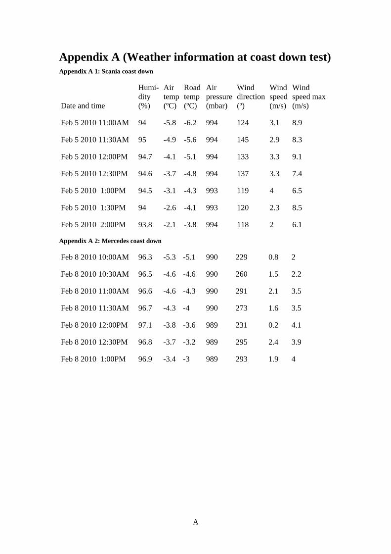
A
Appendix A (Weather information at coast down test) Appendix A 1: Scania coast down
Date and time
Humi-
dity
(%)
Air
temp
(ºC)
Road
temp
(ºC)
Air
pressure
(mbar)
Wind
direction
(º)
Wind
speed
(m/s)
Wind
speed max
(m/s)
Feb 5 2010 11:00AM 94 -5.8 -6.2 994 124 3.1 8.9
Feb 5 2010 11:30AM 95 -4.9 -5.6 994 145 2.9 8.3
Feb 5 2010 12:00PM 94.7 -4.1 -5.1 994 133 3.3 9.1
Feb 5 2010 12:30PM 94.6 -3.7 -4.8 994 137 3.3 7.4
Feb 5 2010 1:00PM 94.5 -3.1 -4.3 993 119 4 6.5
Feb 5 2010 1:30PM 94 -2.6 -4.1 993 120 2.3 8.5
Feb 5 2010 2:00PM 93.8 -2.1 -3.8 994 118 2 6.1
Appendix A 2: Mercedes coast down
Feb 8 2010 10:00AM 96.3 -5.3 -5.1 990 229 0.8 2
Feb 8 2010 10:30AM 96.5 -4.6 -4.6 990 260 1.5 2.2
Feb 8 2010 11:00AM 96.6 -4.6 -4.3 990 291 2.1 3.5
Feb 8 2010 11:30AM 96.7 -4.3 -4 990 273 1.6 3.5
Feb 8 2010 12:00PM 97.1 -3.8 -3.6 989 231 0.2 4.1
Feb 8 2010 12:30PM 96.8 -3.7 -3.2 989 295 2.4 3.9
Feb 8 2010 1:00PM 96.9 -3.4 -3 989 293 1.9 4
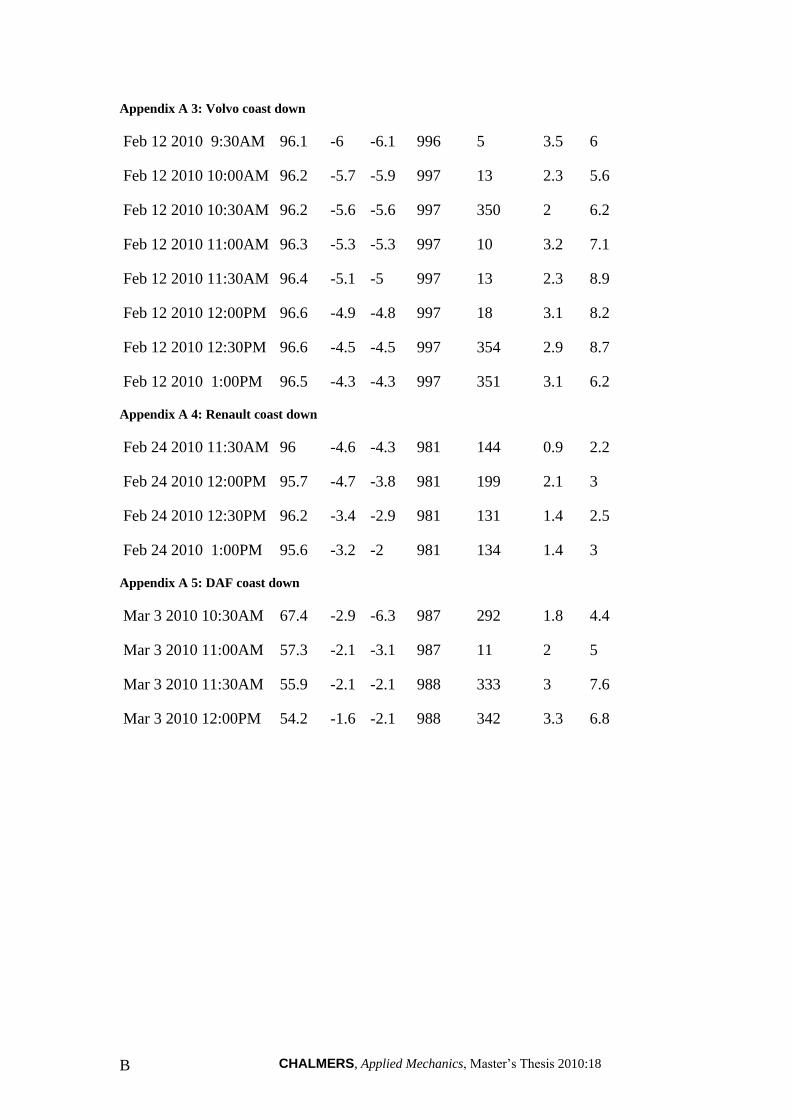
CHALMERS, Applied Mechanics, Master’s Thesis 2010:18 B
Appendix A 3: Volvo coast down
Feb 12 2010 9:30AM 96.1 -6 -6.1 996 5 3.5 6
Feb 12 2010 10:00AM 96.2 -5.7 -5.9 997 13 2.3 5.6
Feb 12 2010 10:30AM 96.2 -5.6 -5.6 997 350 2 6.2
Feb 12 2010 11:00AM 96.3 -5.3 -5.3 997 10 3.2 7.1
Feb 12 2010 11:30AM 96.4 -5.1 -5 997 13 2.3 8.9
Feb 12 2010 12:00PM 96.6 -4.9 -4.8 997 18 3.1 8.2
Feb 12 2010 12:30PM 96.6 -4.5 -4.5 997 354 2.9 8.7
Feb 12 2010 1:00PM 96.5 -4.3 -4.3 997 351 3.1 6.2
Appendix A 4: Renault coast down
Feb 24 2010 11:30AM 96 -4.6 -4.3 981 144 0.9 2.2
Feb 24 2010 12:00PM 95.7 -4.7 -3.8 981 199 2.1 3
Feb 24 2010 12:30PM 96.2 -3.4 -2.9 981 131 1.4 2.5
Feb 24 2010 1:00PM 95.6 -3.2 -2 981 134 1.4 3
Appendix A 5: DAF coast down
Mar 3 2010 10:30AM 67.4 -2.9 -6.3 987 292 1.8 4.4
Mar 3 2010 11:00AM 57.3 -2.1 -3.1 987 11 2 5
Mar 3 2010 11:30AM 55.9 -2.1 -2.1 988 333 3 7.6
Mar 3 2010 12:00PM 54.2 -1.6 -2.1 988 342 3.3 6.8
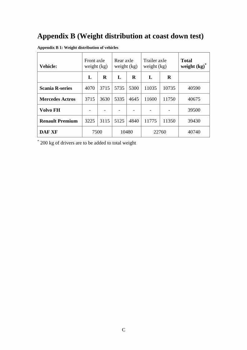
C
Appendix B (Weight distribution at coast down test)
Appendix B 1: Weight distribution of vehicles
Vehicle:
Front axle
weight (kg)
Rear axle
weight (kg)
Trailer axle
weight (kg)
Total
weight (kg)*
L R L R L R
Scania R-series 4070 3715 5735 5300 11035 10735 40590
Mercedes Actros 3715 3630 5335 4645 11600 11750 40675
Volvo FH - - - - - - 39500
Renault Premium 3225 3115 5125 4840 11775 11350 39430
DAF XF 7500 10480 22760 40740
* 200 kg of drivers are to be added to total weight
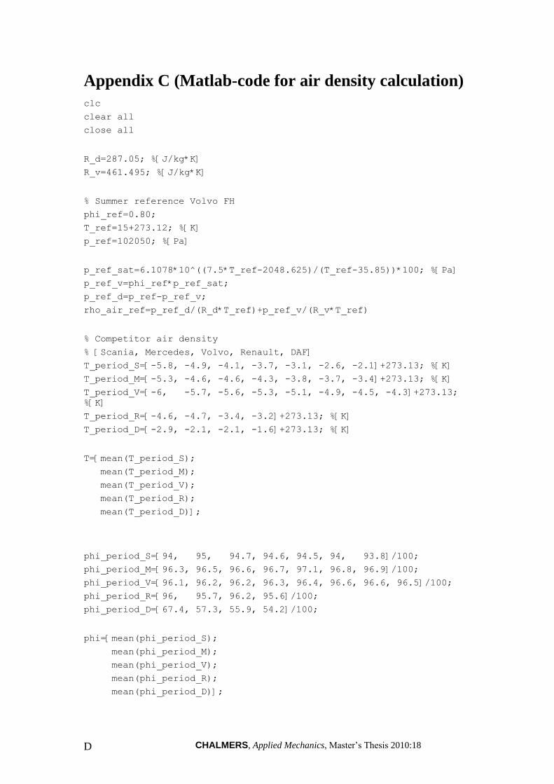
CHALMERS, Applied Mechanics, Master’s Thesis 2010:18 D
Appendix C (Matlab-code for air density calculation)
clc
clear all
close all
R_d=287.05; %[J/kg*K]
R_v=461.495; %[J/kg*K]
% Summer reference Volvo FH
phi_ref=0.80;
T_ref=15+273.12; %[K]
p_ref=102050; %[Pa]
p_ref_sat=6.1078*10^((7.5*T_ref-2048.625)/(T_ref-35.85))*100; %[Pa]
p_ref_v=phi_ref*p_ref_sat;
p_ref_d=p_ref-p_ref_v;
rho_air_ref=p_ref_d/(R_d*T_ref)+p_ref_v/(R_v*T_ref)
% Competitor air density
% [Scania, Mercedes, Volvo, Renault, DAF]
T_period_S=[-5.8, -4.9, -4.1, -3.7, -3.1, -2.6, -2.1]+273.13; %[K]
T_period_M=[-5.3, -4.6, -4.6, -4.3, -3.8, -3.7, -3.4]+273.13; %[K]
T_period_V=[-6, -5.7, -5.6, -5.3, -5.1, -4.9, -4.5, -4.3]+273.13;
%[K]
T_period_R=[-4.6, -4.7, -3.4, -3.2]+273.13; %[K]
T_period_D=[-2.9, -2.1, -2.1, -1.6]+273.13; %[K]
T=[mean(T_period_S);
mean(T_period_M);
mean(T_period_V);
mean(T_period_R);
mean(T_period_D)];
phi_period_S=[94, 95, 94.7, 94.6, 94.5, 94, 93.8]/100;
phi_period_M=[96.3, 96.5, 96.6, 96.7, 97.1, 96.8, 96.9]/100;
phi_period_V=[96.1, 96.2, 96.2, 96.3, 96.4, 96.6, 96.6, 96.5]/100;
phi_period_R=[96, 95.7, 96.2, 95.6]/100;
phi_period_D=[67.4, 57.3, 55.9, 54.2]/100;
phi=[mean(phi_period_S);
mean(phi_period_M);
mean(phi_period_V);
mean(phi_period_R);
mean(phi_period_D)];

E
p_period_S=[994, 994, 994, 994, 993, 993, 994]*100; %[Pa]
p_period_M=[990, 990, 990, 990, 989, 989, 989]*100; %[Pa]
p_period_V=[996, 997, 997, 997, 997, 997, 997, 997]*100; %[Pa]
p_period_R=[981, 981, 981, 981]*100; %[Pa]
p_period_D=[987, 987, 988, 988]*100; %[Pa]
p=[mean(p_period_S);
mean(p_period_M);
mean(p_period_V);
mean(p_period_R);
mean(p_period_D)];
p_sat=6.1078.*10.^((7.5.*T-2048.625)./(T-35.85)).*100; %[Pa]
p_v=phi.*p_sat;
p_d=p-p_v;
rho_air=p_d./(R_d.*T)+p_v./(R_v.*T)
%Comparison
Percent=(1-rho_air_ref./rho_air).*100
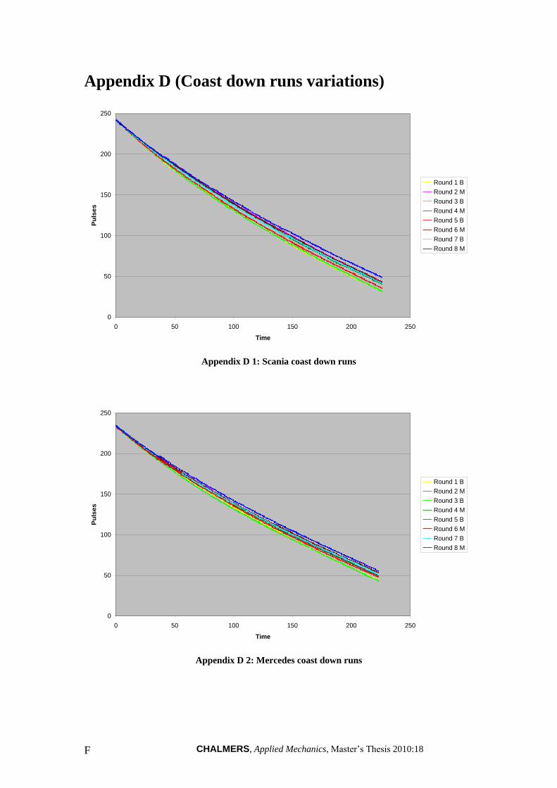
CHALMERS, Applied Mechanics, Master’s Thesis 2010:18 F
Appendix D (Coast down runs variations)
0
50
100
150
200
250
0 50 100 150 200 250
Time
Pu
lse
s
Round 1 B
Round 2 M
Round 3 B
Round 4 M
Round 5 B
Round 6 M
Round 7 B
Round 8 M
Appendix D 1: Scania coast down runs
0
50
100
150
200
250
0 50 100 150 200 250
Time
Pu
lse
s
Round 1 B
Round 2 M
Round 3 B
Round 4 M
Round 5 B
Round 6 M
Round 7 B
Round 8 M
Appendix D 2: Mercedes coast down runs
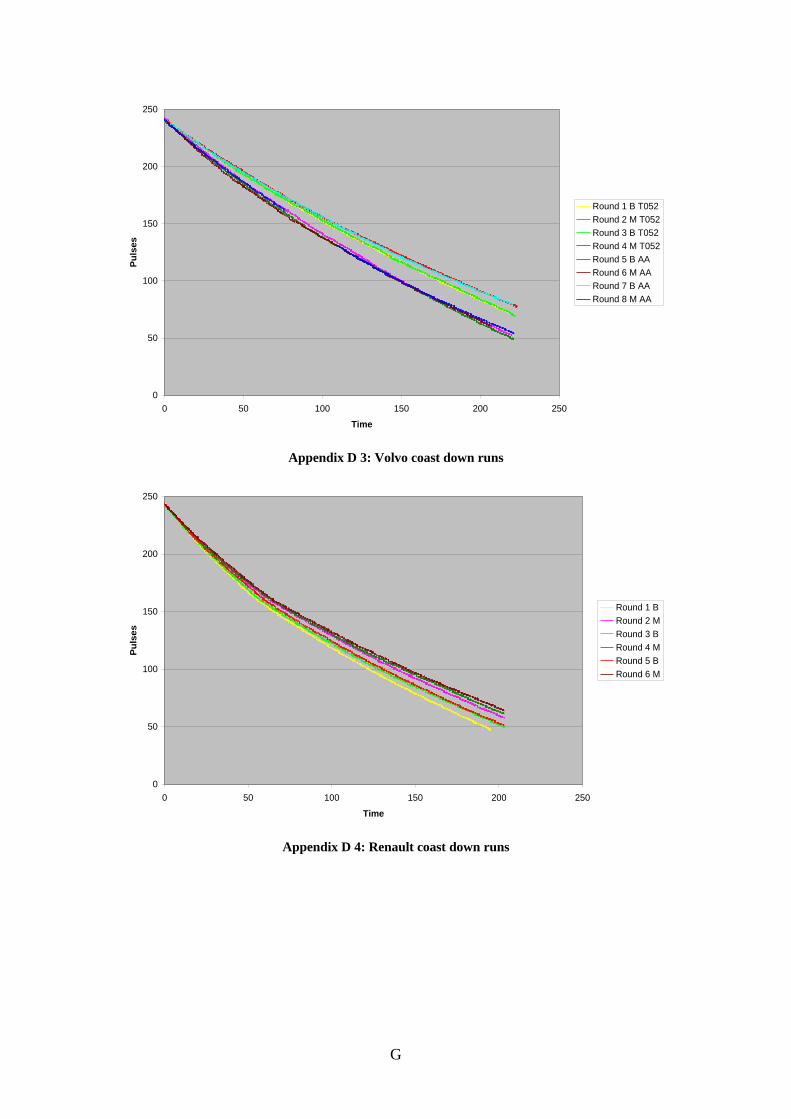
G
0
50
100
150
200
250
0 50 100 150 200 250
Time
Pu
lse
s
Round 1 B T052
Round 2 M T052
Round 3 B T052
Round 4 M T052
Round 5 B AA
Round 6 M AA
Round 7 B AA
Round 8 M AA
Appendix D 3: Volvo coast down runs
0
50
100
150
200
250
0 50 100 150 200 250
Time
Pu
lse
s
Round 1 B
Round 2 M
Round 3 B
Round 4 M
Round 5 B
Round 6 M
Appendix D 4: Renault coast down runs
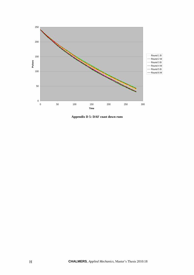
CHALMERS, Applied Mechanics, Master’s Thesis 2010:18 H
0
50
100
150
200
250
0 50 100 150 200 250 300
Time
Pu
lse
s
Round 1 B
Round 2 M
Round 3 B
Round 4 M
Round 5 B
Round 6 M
Appendix D 5: DAF coast down runs
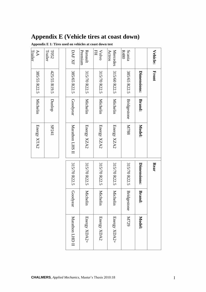
CHALMERS, Applied Mechanics, Master’s Thesis 2010:18 I
Appendix E (Vehicle tires at coast down) Appendix E 1: Tires used on vehicles at coast down test
AA
Trailer
T052
Trailer
DA
F X
F
Ren
ault
Prem
ium
Volv
o
FH
Merced
es
Actro
s
Scan
ia
R480
Veh
icle:
385/5
5 R
22.5
425/5
5 R
19.5
385/6
5 R
22.5
315/7
0 R
22.5
315/7
0 R
22.5
315/6
0 R
22.5
385/6
5 R
22.5
Dim
ensio
ns:
Fro
nt
Mich
elin
Dunlo
p
Goodyear
Mich
elin
Mich
elin
Mich
elin
Brid
gesto
ne
Bra
nd
:
Energ
y X
TA
2
SP
241
Marath
on L
HS
II
Energ
y X
ZA
2
Energ
y X
ZA
2
Energ
y X
ZA
2
M788
Mod
el:
315/7
0 R
22.5
315/7
0 R
22.5
315/7
0 R
22.5
315/7
0 R
22.5
315/7
0 R
22.5
Dim
ensio
ns:
Rea
r
Goodyear
Mich
elin
Mich
elin
Mich
elin
Brid
gesto
ne
Bra
nd
:
Marath
on L
HD
II
Energ
y X
DA
2+
Energ
y X
DA
2
Energ
y X
DA
2+
M729
Mod
el:
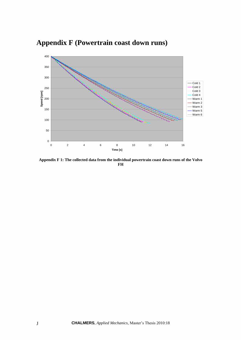
CHALMERS, Applied Mechanics, Master’s Thesis 2010:18 J
Appendix F (Powertrain coast down runs)
0
50
100
150
200
250
300
350
400
0 2 4 6 8 10 12 14 16
Time [s]
Sp
ee
d [
rpm
]
Cold 1
Cold 2
Cold 3
Cold 4
Warm 1
Warm 2
Warm 3
Warm 5
Warm 6
Appendix F 1: The collected data from the individual powertrain coast down runs of the Volvo
FH
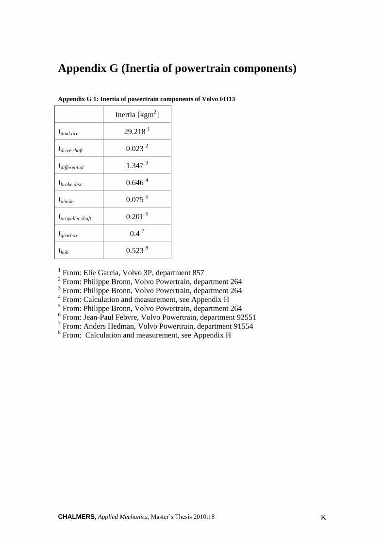
CHALMERS, Applied Mechanics, Master’s Thesis 2010:18 K
Appendix G (Inertia of powertrain components)
Appendix G 1: Inertia of powertrain components of Volvo FH13
Inertia [kgm2]
Idual tire 29.218 1
Idrive shaft 0.023 2
Idifferential 1.347 3
Ibrake disc 0.646 4
Ipinion 0.075 5
Ipropeller shaft 0.201 6
Igearbox 0.4 7
Ihub 0.523 8
1 From: Elie Garcia, Volvo 3P, department 857
2 From: Philippe Bronn, Volvo Powertrain, department 264
3 From: Philippe Bronn, Volvo Powertrain, department 264
4 From: Calculation and measurement, see Appendix H
5 From: Philippe Bronn, Volvo Powertrain, department 264
6 From: Jean-Paul Febvre, Volvo Powertrain, department 92551
7 From: Anders Hedman, Volvo Powertrain, department 91554
8 From: Calculation and measurement, see Appendix H
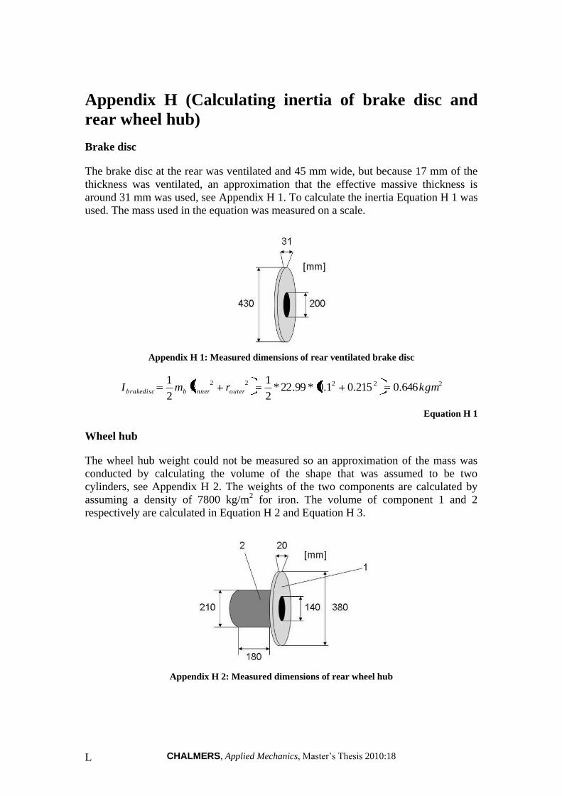
CHALMERS, Applied Mechanics, Master’s Thesis 2010:18 L
Appendix H (Calculating inertia of brake disc and
rear wheel hub)
Brake disc
The brake disc at the rear was ventilated and 45 mm wide, but because 17 mm of the
thickness was ventilated, an approximation that the effective massive thickness is
around 31 mm was used, see Appendix H 1. To calculate the inertia Equation H 1 was
used. The mass used in the equation was measured on a scale.
Appendix H 1: Measured dimensions of rear ventilated brake disc
22222646.0215.01.0*99.22*
2
1
2
1kgmrrmI outerinnerbbrakedisc
Equation H 1
Wheel hub
The wheel hub weight could not be measured so an approximation of the mass was
conducted by calculating the volume of the shape that was assumed to be two
cylinders, see Appendix H 2. The weights of the two components are calculated by
assuming a density of 7800 kg/m2 for iron. The volume of component 1 and 2
respectively are calculated in Equation H 2 and Equation H 3.
Appendix H 2: Measured dimensions of rear wheel hub
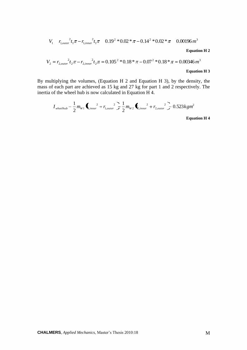
CHALMERS, Applied Mechanics, Master’s Thesis 2010:18 M
322
1
2
,11
2
,11 00196.0*02.0*14.0*02.0*19.0 mtrtrV innerouter
Equation H 2
322
2
2
,22
2
,22 00346.0*18.0*07.0*18.0*105.0 mtrtrV innerouter
Equation H 3
By multiplying the volumes, (Equation H 2 and Equation H 3), by the density, the
mass of each part are achieved as 15 kg and 27 kg for part 1 and 2 respectively. The
inertia of the wheel hub is now calculated in Equation H 4.
22
,2
2
,22
2
,1
2
,11 523.02
1
2
1kgmrrmrrmI outerinnerWouterinnerWwheelhub
Equation H 4
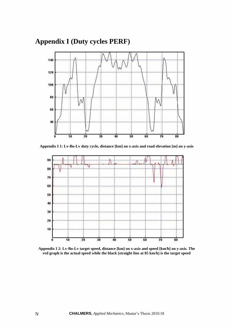
CHALMERS, Applied Mechanics, Master’s Thesis 2010:18 N
Appendix I (Duty cycles PERF)
Appendix I 1: Lv-Bo-Lv duty cycle, distance [km] on x-axis and road elevation [m] on y-axis
Appendix I 2: Lv-Bo-Lv target speed, distance [km] on x-axis and speed [km/h] on y-axis. The
red graph is the actual speed while the black (straight line at 85 km/h) is the target speed
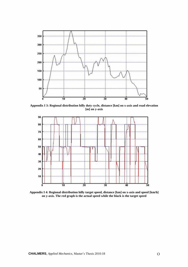
CHALMERS, Applied Mechanics, Master’s Thesis 2010:18 O
Appendix I 3: Regional distribution hilly duty cycle, distance [km] on x-axis and road elevation
[m] on y-axis
Appendix I 4: Regional distribution hilly target speed, distance [km] on x-axis and speed [km/h]
on y-axis. The red graph is the actual speed while the black is the target speed
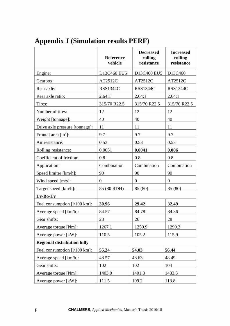
CHALMERS, Applied Mechanics, Master’s Thesis 2010:18 P
Appendix J (Simulation results PERF)
Reference
vehicle
Decreased
rolling
resistance
Increased
rolling
resistance
Engine: D13C460 EU5 D13C460 EU5 D13C460
EU5 Gearbox: AT2512C AT2512C AT2512C
Rear axle: RSS1344C RSS1344C RSS1344C
Rear axle ratio: 2.64:1 2.64:1 2.64:1
Tires: 315/70 R22.5 315/70 R22.5 315/70 R22.5
Number of tires: 12 12 12
Weight [tonnage]: 40 40 40
Drive axle pressure [tonnage]: 11 11 11
Frontal area [m2]: 9.7 9.7 9.7
Air resistance: 0.53 0.53 0.53
Rolling resistance: 0.0051 0.0041 0.006
Coefficient of friction: 0.8 0.8 0.8
Application: Combination Combination Combination
Speed limiter [km/h]: 90 90 90
Wind speed [m/s]: 0 0 0
Target speed [km/h]: 85 (80 RDH) 85 (80) 85 (80)
Lv-Bo-Lv
Fuel consumption [l/100 km]: 30.96 29.42 32.49
Average speed [km/h]: 84.57 84.78 84.36
Gear shifts: 28 26 28
Average torque [Nm]: 1267.1 1250.9 1290.3
Average power [kW]: 110.5 105.2 115.9
Regional distribution hilly
Fuel consumption [l/100 km]: 55.24 54.03 56.44
Average speed [km/h]: 48.57 48.63 48.49
Gear shifts: 102 102 104
Average torque [Nm]: 1403.0 1401.8 1433.5
Average power [kW]: 111.5 109.2 113.8
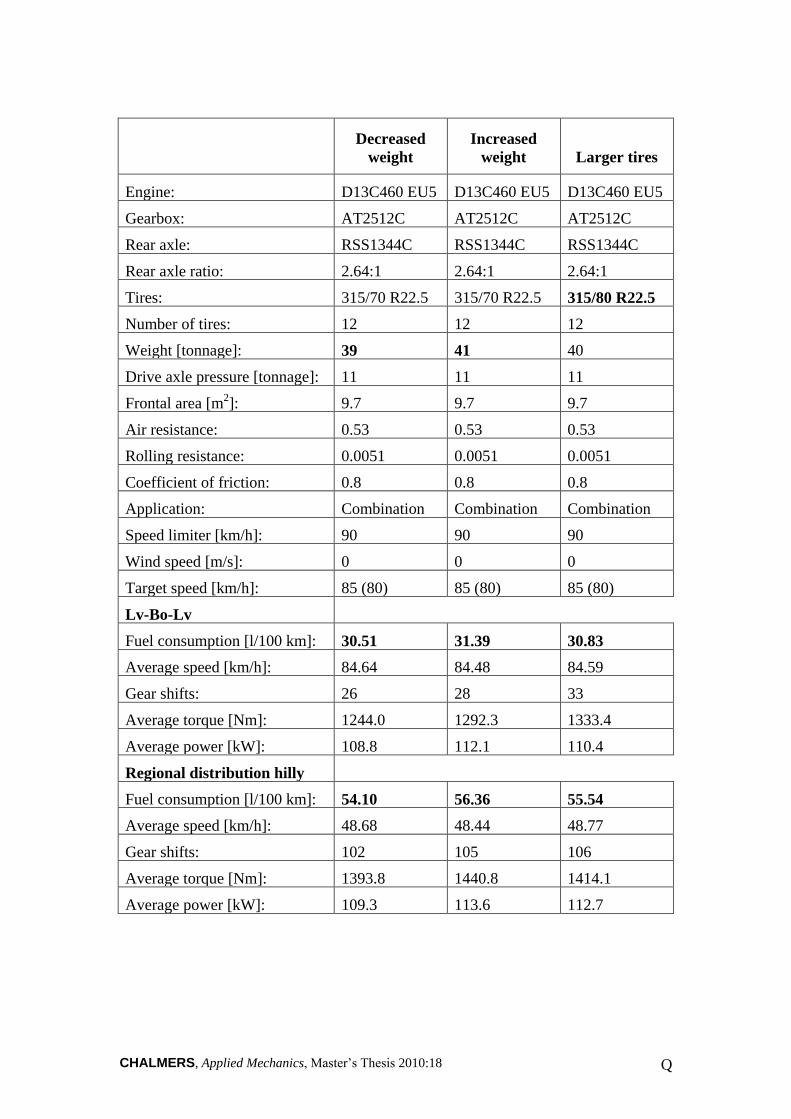
CHALMERS, Applied Mechanics, Master’s Thesis 2010:18 Q
Decreased
weight
Increased
weight Larger tires
Engine: D13C460 EU5 D13C460 EU5 D13C460 EU5
Gearbox: AT2512C AT2512C AT2512C
Rear axle: RSS1344C RSS1344C RSS1344C
Rear axle ratio: 2.64:1 2.64:1 2.64:1
Tires: 315/70 R22.5 315/70 R22.5 315/80 R22.5
Number of tires: 12 12 12
Weight [tonnage]: 39 41 40
Drive axle pressure [tonnage]: 11 11 11
Frontal area [m2]: 9.7 9.7 9.7
Air resistance: 0.53 0.53 0.53
Rolling resistance: 0.0051 0.0051 0.0051
Coefficient of friction: 0.8 0.8 0.8
Application: Combination Combination Combination
Speed limiter [km/h]: 90 90 90
Wind speed [m/s]: 0 0 0
Target speed [km/h]: 85 (80) 85 (80) 85 (80)
Lv-Bo-Lv
Fuel consumption [l/100 km]: 30.51 31.39 30.83
Average speed [km/h]: 84.64 84.48 84.59
Gear shifts: 26 28 33
Average torque [Nm]: 1244.0 1292.3 1333.4
Average power [kW]: 108.8 112.1 110.4
Regional distribution hilly
Fuel consumption [l/100 km]: 54.10 56.36 55.54
Average speed [km/h]: 48.68 48.44 48.77
Gear shifts: 102 105 106
Average torque [Nm]: 1393.8 1440.8 1414.1
Average power [kW]: 109.3 113.6 112.7

CHALMERS, Applied Mechanics, Master’s Thesis 2010:18 R
Smaller tires
Decreased
drag
Increased
drag
Engine: D13C460 EU5 D13C460 EU5 D13C460 EU5
Gearbox: AT2512C AT2512C AT2512C
Rear axle: RSS1344C RSS1344C RSS1344C
Rear axle ratio: 2.64:1 2.64:1 2.64:1
Tires: 315/60 R22.5 315/70 R22.5 315/70 R22.5
Number of tires: 12 12 12
Weight [tonnage]: 40 40 40
Drive axle pressure [tonnage]: 11 11 11
Frontal area [m2]: 9.7 9.7 9.7
Air resistance: 0.53 0.5 0.56
Rolling resistance: 0.0051 0.0051 0.0051
Coefficient of friction: 0.8 0.8 0.8
Application: Combination Combination Combination
Speed limiter [km/h]: 90 90 90
Wind speed [m/s]: 0 0 0
Target speed [km/h]: 85 (80) 85 (80) 85 (80)
Lv-Bo-Lv
Fuel consumption [l/100 km]: 31.16 30.48 31.42
Average speed [km/h]: 84.59 84.61 84.50
Gear shifts: 24 28 28
Average torque [Nm]: 1211.7 1260.2 1276.2
Average power [kW]: 110.8 108.8 112.1
Regional distribution hilly
Fuel consumption [l/100 km]: 55.47 55.00 55.28
Average speed [km/h]: 48.37 48.57 48.53
Gear shifts: 93 104 104
Average torque [Nm]: 1355.4 1419.2 1423.8
Average power [kW]: 111.1 111.2 111.7
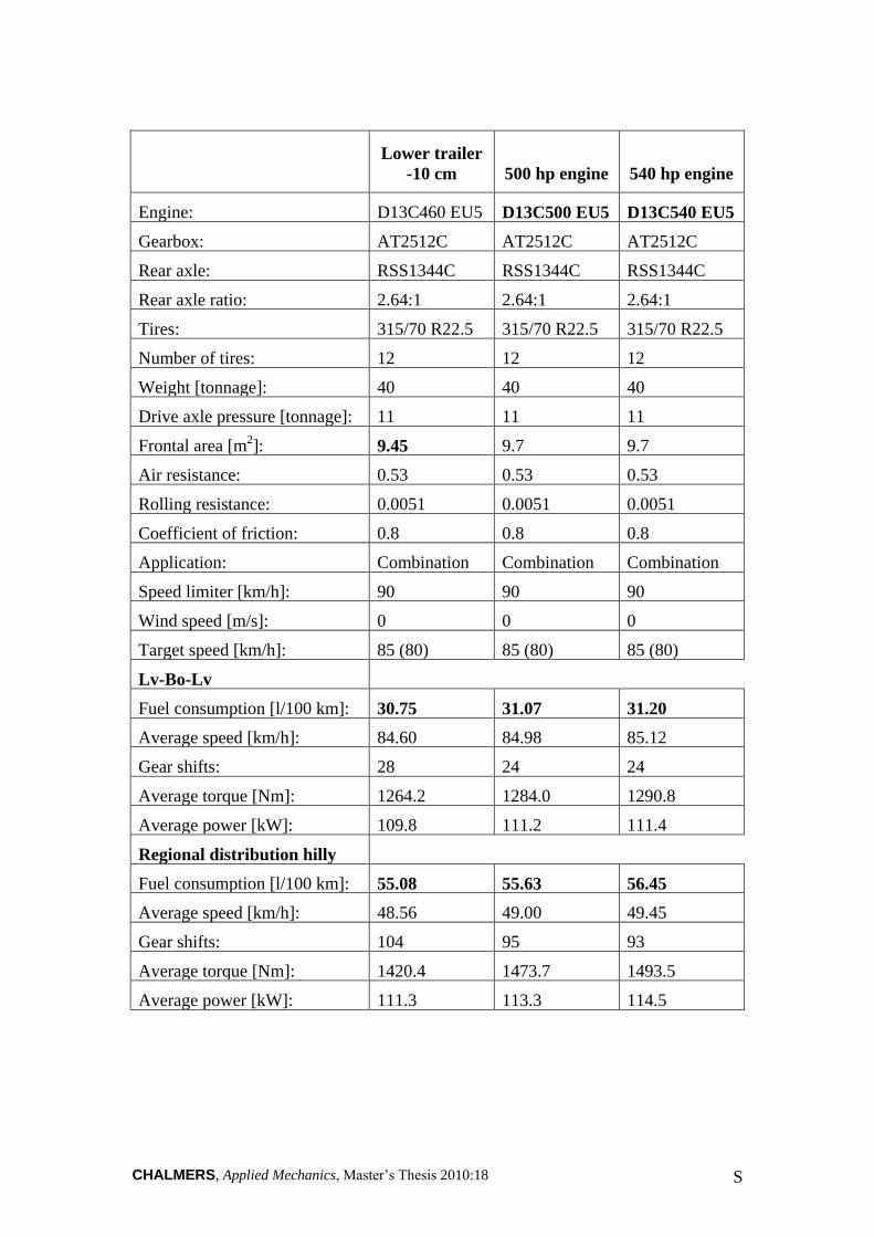
CHALMERS, Applied Mechanics, Master’s Thesis 2010:18 S
Lower trailer
-10 cm 500 hp engine 540 hp engine
Engine: D13C460 EU5 D13C500 EU5 D13C540 EU5
Gearbox: AT2512C AT2512C AT2512C
Rear axle: RSS1344C RSS1344C RSS1344C
Rear axle ratio: 2.64:1 2.64:1 2.64:1
Tires: 315/70 R22.5 315/70 R22.5 315/70 R22.5
Number of tires: 12 12 12
Weight [tonnage]: 40 40 40
Drive axle pressure [tonnage]: 11 11 11
Frontal area [m2]: 9.45 9.7 9.7
Air resistance: 0.53 0.53 0.53
Rolling resistance: 0.0051 0.0051 0.0051
Coefficient of friction: 0.8 0.8 0.8
Application: Combination Combination Combination
Speed limiter [km/h]: 90 90 90
Wind speed [m/s]: 0 0 0
Target speed [km/h]: 85 (80) 85 (80) 85 (80)
Lv-Bo-Lv
Fuel consumption [l/100 km]: 30.75 31.07 31.20
Average speed [km/h]: 84.60 84.98 85.12
Gear shifts: 28 24 24
Average torque [Nm]: 1264.2 1284.0 1290.8
Average power [kW]: 109.8 111.2 111.4
Regional distribution hilly
Fuel consumption [l/100 km]: 55.08 55.63 56.45
Average speed [km/h]: 48.56 49.00 49.45
Gear shifts: 104 95 93
Average torque [Nm]: 1420.4 1473.7 1493.5
Average power [kW]: 111.3 113.3 114.5
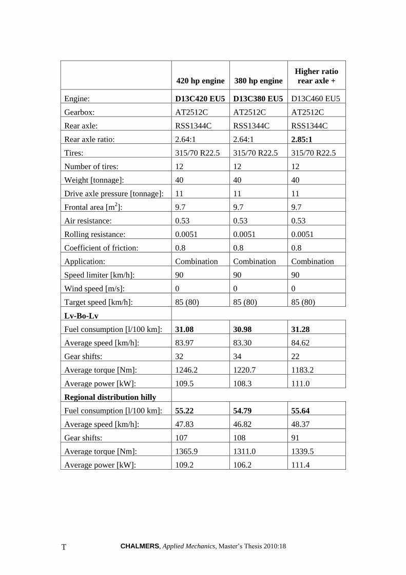
CHALMERS, Applied Mechanics, Master’s Thesis 2010:18 T
420 hp engine 380 hp engine
Higher ratio
rear axle +
Engine: D13C420 EU5 D13C380 EU5 D13C460 EU5
Gearbox: AT2512C AT2512C AT2512C
Rear axle: RSS1344C RSS1344C RSS1344C
Rear axle ratio: 2.64:1 2.64:1 2.85:1
Tires: 315/70 R22.5 315/70 R22.5 315/70 R22.5
Number of tires: 12 12 12
Weight [tonnage]: 40 40 40
Drive axle pressure [tonnage]: 11 11 11
Frontal area [m2]: 9.7 9.7 9.7
Air resistance: 0.53 0.53 0.53
Rolling resistance: 0.0051 0.0051 0.0051
Coefficient of friction: 0.8 0.8 0.8
Application: Combination Combination Combination
Speed limiter [km/h]: 90 90 90
Wind speed [m/s]: 0 0 0
Target speed [km/h]: 85 (80) 85 (80) 85 (80)
Lv-Bo-Lv
Fuel consumption [l/100 km]: 31.08 30.98 31.28
Average speed [km/h]: 83.97 83.30 84.62
Gear shifts: 32 34 22
Average torque [Nm]: 1246.2 1220.7 1183.2
Average power [kW]: 109.5 108.3 111.0
Regional distribution hilly
Fuel consumption [l/100 km]: 55.22 54.79 55.64
Average speed [km/h]: 47.83 46.82 48.37
Gear shifts: 107 108 91
Average torque [Nm]: 1365.9 1311.0 1339.5
Average power [kW]: 109.2 106.2 111.4
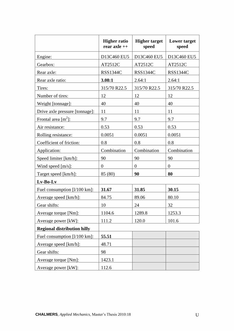
CHALMERS, Applied Mechanics, Master’s Thesis 2010:18 U
Higher ratio
rear axle ++
Higher target
speed
Lower target
speed
Engine: D13C460 EU5 D13C460 EU5 D13C460 EU5
Gearbox: AT2512C AT2512C AT2512C
Rear axle: RSS1344C RSS1344C RSS1344C
Rear axle ratio: 3.08:1 2.64:1 2.64:1
Tires: 315/70 R22.5 315/70 R22.5 315/70 R22.5
Number of tires: 12 12 12
Weight [tonnage]: 40 40 40
Drive axle pressure [tonnage]: 11 11 11
Frontal area [m2]: 9.7 9.7 9.7
Air resistance: 0.53 0.53 0.53
Rolling resistance: 0.0051 0.0051 0.0051
Coefficient of friction: 0.8 0.8 0.8
Application: Combination Combination Combination
Speed limiter [km/h]: 90 90 90
Wind speed [m/s]: 0 0 0
Target speed [km/h]: 85 (80) 90 80
Lv-Bo-Lv
Fuel consumption [l/100 km]: 31.67 31.85 30.15
Average speed [km/h]: 84.75 89.06 80.10
Gear shifts: 10 24 32
Average torque [Nm]: 1104.6 1289.8 1253.3
Average power [kW]: 111.2 120.0 101.6
Regional distribution hilly
Fuel consumption [l/100 km]: 55.51
Average speed [km/h]: 48.71
Gear shifts: 98
Average torque [Nm]: 1423.1
Average power [kW]: 112.6

CHALMERS, Applied Mechanics, Master’s Thesis 2010:18 V
2.5 m/s wind
speed
5.0 m/s wind
speed
Engine: D13C460 EU5 D13C460 EU5
Gearbox: AT2512C AT2512C
Rear axle: RSS1344C RSS1344C
Rear axle ratio: 2.64:1 2.64:1
Tires: 315/70 R22.5 315/70 R22.5
Number of tires: 12 12
Weight [tonnage]: 40 40
Drive axle pressure [tonnage]: 11 11
Frontal area [m2]: 9.7 9.7
Air resistance: 0.53 0.53
Rolling resistance: 0.0051 0.0051
Coefficient of friction: 0.8 0.8
Application: Combination Combination
Speed limiter [km/h]: 90 90
Wind speed [m/s]: 2.5 5.0
Target speed [km/h]: 85 (80) 85 (80)
Lv-Bo-Lv
Fuel consumption [l/100 km]: 32.82 34.93
Average speed [km/h]: 84.33 84.04
Gear shifts: 28 30
Average torque [Nm]: 1297.1 1327.0
Average power [kW]: 117.1 124.5
Regional distribution hilly
Fuel consumption [l/100 km]: 56.25 57.32
Average speed [km/h]: 48.52 48.41
Gear shifts: 104 104
Average torque [Nm]: 1428.3
1439.4
Average power [kW]: 113.4 115.5
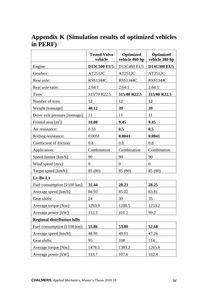
CHALMERS, Applied Mechanics, Master’s Thesis 2010:18 W
Appendix K (Simulation results of optimized vehicles
in PERF)
Tested Volvo
vehicle
Optimized
vehicle 460 hp
Optimized
vehicle 380 hp
Engine: D13C500 EU5 D13C460 EU5 D13C380 EU5
Gearbox: AT2512C AT2512C AT2512C
Rear axle: RSS1344C RSS1344C RSS1344C
Rear axle ratio: 2.64:1 2.64:1 2.64:1
Tires: 315/70 R22.5 315/80 R22.5 315/80 R22.5
Number of tires: 12 12 12
Weight [tonnage]: 40.12 39 39
Drive axle pressure [tonnage]: 11 11 11
Frontal area [m2]: 10.08 9.45 9.45
Air resistance: 0.53 0.5 0.5
Rolling resistance: 0.0051 0.0041 0.0041
Coefficient of friction: 0.8 0.8 0.8
Application: Combination Combination Combination
Speed limiter [km/h]: 90 90 90
Wind speed [m/s]: 0 0 0
Target speed [km/h]: 85 (80) 85 (80) 85 (80)
Lv-Bo-Lv
Fuel consumption [l/100 km]: 31.44 28.23 28.25
Average speed [km/h]: 84.93 85.02 83.81
Gear shifts: 24 30 35
Average torque [Nm]: 1293.3 1280.5 1233.2
Average power [kW]: 112.5 101.2 99.2
Regional distribution hilly
Fuel consumption [l/100 km]: 55.86 53.00 52.68
Average speed [km/h]: 48.95 49.01 47.26
Gear shifts: 95 108 114
Average torque [Nm]: 1478.5 1383.2 1265.8
Average power [kW]: 113.7 107.6 102.4
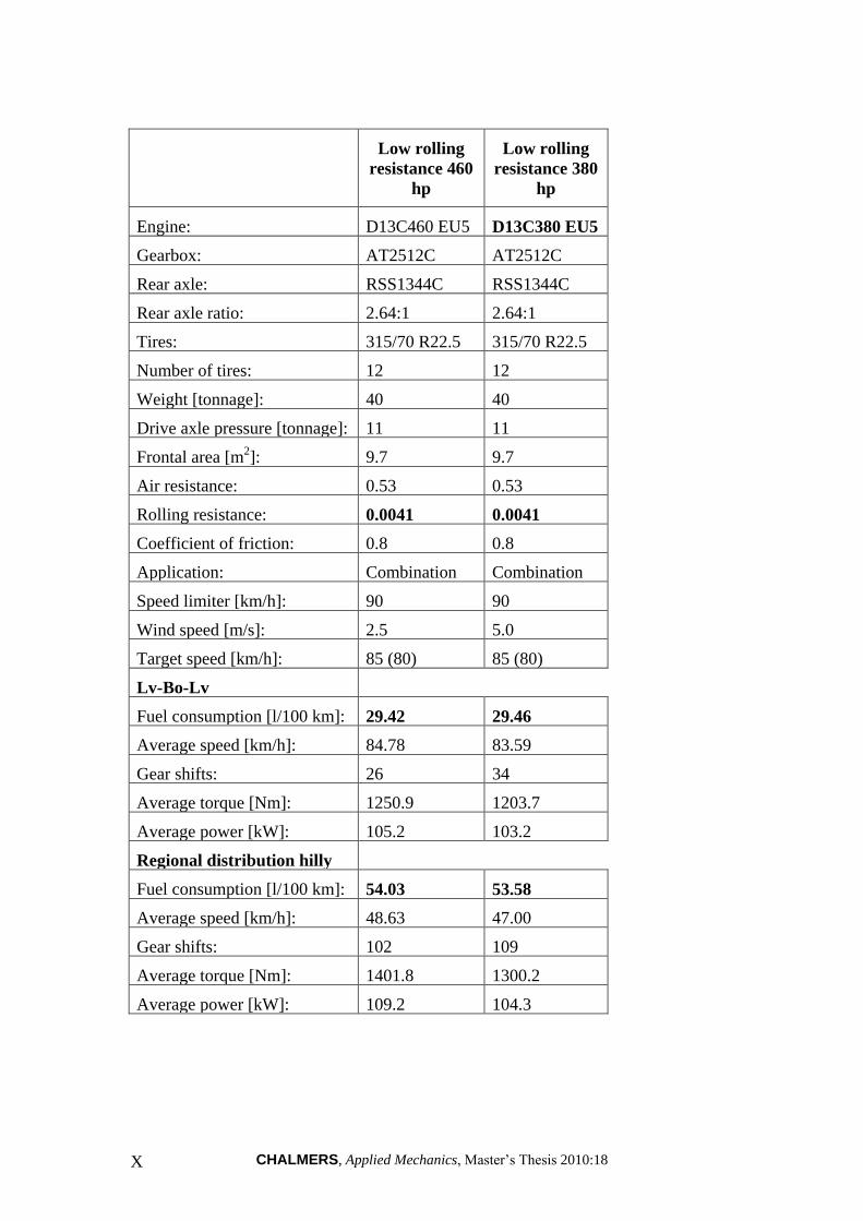
CHALMERS, Applied Mechanics, Master’s Thesis 2010:18 X
Low rolling
resistance 460
hp
Low rolling
resistance 380
hp
Engine: D13C460 EU5 D13C380 EU5
Gearbox: AT2512C AT2512C
Rear axle: RSS1344C RSS1344C
Rear axle ratio: 2.64:1 2.64:1
Tires: 315/70 R22.5 315/70 R22.5
Number of tires: 12 12
Weight [tonnage]: 40 40
Drive axle pressure [tonnage]: 11 11
Frontal area [m2]: 9.7 9.7
Air resistance: 0.53 0.53
Rolling resistance: 0.0041 0.0041
Coefficient of friction: 0.8 0.8
Application: Combination Combination
Speed limiter [km/h]: 90 90
Wind speed [m/s]: 2.5 5.0
Target speed [km/h]: 85 (80) 85 (80)
Lv-Bo-Lv
Fuel consumption [l/100 km]: 29.42 29.46
Average speed [km/h]: 84.78 83.59
Gear shifts: 26 34
Average torque [Nm]: 1250.9 1203.7
Average power [kW]: 105.2 103.2
Regional distribution hilly
Fuel consumption [l/100 km]: 54.03 53.58
Average speed [km/h]: 48.63 47.00
Gear shifts: 102 109
Average torque [Nm]: 1401.8
1300.2
Average power [kW]: 109.2 104.3
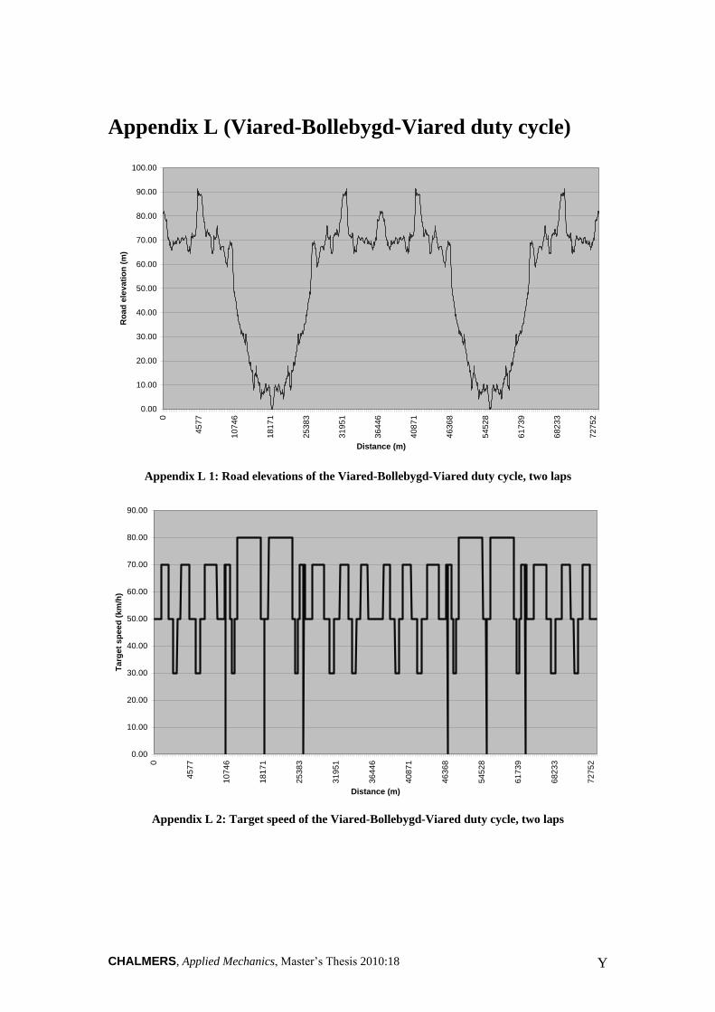
CHALMERS, Applied Mechanics, Master’s Thesis 2010:18 Y
Appendix L (Viared-Bollebygd-Viared duty cycle)
0.00
10.00
20.00
30.00
40.00
50.00
60.00
70.00
80.00
90.00
100.000
45
77
10
74
6
18
17
1
25
38
3
31
95
1
36
44
6
40
87
1
46
36
8
54
52
8
61
73
9
68
23
3
72
75
2
Distance (m)
Ro
ad
ele
va
tio
n (
m)
Appendix L 1: Road elevations of the Viared-Bollebygd-Viared duty cycle, two laps
0.00
10.00
20.00
30.00
40.00
50.00
60.00
70.00
80.00
90.00
0
45
77
10
74
6
18
17
1
25
38
3
31
95
1
36
44
6
40
87
1
46
36
8
54
52
8
61
73
9
68
23
3
72
75
2
Distance (m)
Targ
et
sp
ee
d (
km
/h)
Appendix L 2: Target speed of the Viared-Bollebygd-Viared duty cycle, two laps
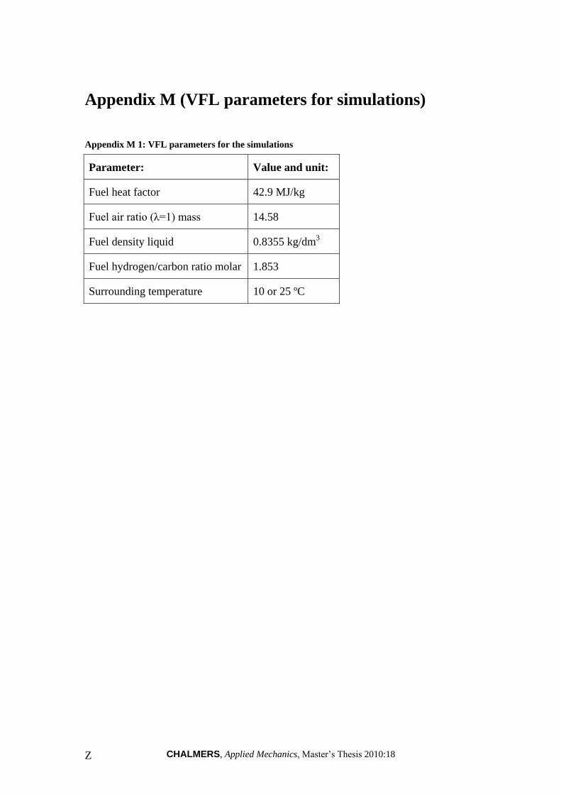
CHALMERS, Applied Mechanics, Master’s Thesis 2010:18 Z
Appendix M (VFL parameters for simulations)
Appendix M 1: VFL parameters for the simulations
Parameter: Value and unit:
Fuel heat factor 42.9 MJ/kg
Fuel air ratio (λ=1) mass 14.58
Fuel density liquid 0.8355 kg/dm3
Fuel hydrogen/carbon ratio molar 1.853
Surrounding temperature 10 or 25 ºC
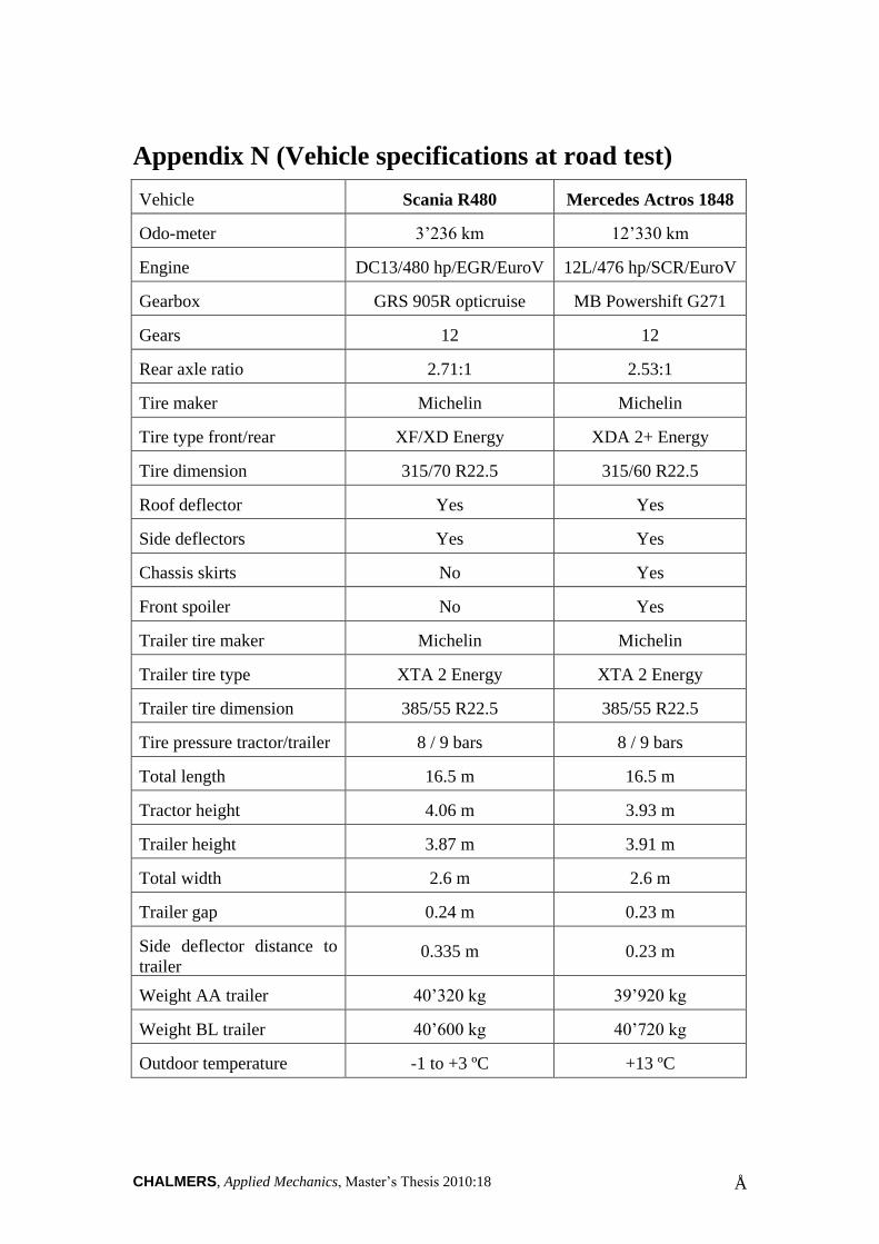
CHALMERS, Applied Mechanics, Master’s Thesis 2010:18 Å
Appendix N (Vehicle specifications at road test)
Vehicle Scania R480 Mercedes Actros 1848
Odo-meter 3’236 km 12’330 km
Engine DC13/480 hp/EGR/EuroV 12L/476 hp/SCR/EuroV
Gearbox GRS 905R opticruise MB Powershift G271
Gears 12 12
Rear axle ratio 2.71:1 2.53:1
Tire maker Michelin Michelin
Tire type front/rear XF/XD Energy XDA 2+ Energy
Tire dimension 315/70 R22.5 315/60 R22.5
Roof deflector Yes Yes
Side deflectors Yes Yes
Chassis skirts No Yes
Front spoiler No Yes
Trailer tire maker Michelin Michelin
Trailer tire type XTA 2 Energy XTA 2 Energy
Trailer tire dimension 385/55 R22.5 385/55 R22.5
Tire pressure tractor/trailer 8 / 9 bars 8 / 9 bars
Total length 16.5 m 16.5 m
Tractor height 4.06 m 3.93 m
Trailer height 3.87 m 3.91 m
Total width 2.6 m 2.6 m
Trailer gap 0.24 m 0.23 m
Side deflector distance to
trailer 0.335 m 0.23 m
Weight AA trailer 40’320 kg 39’920 kg
Weight BL trailer 40’600 kg 40’720 kg
Outdoor temperature -1 to +3 ºC +13 ºC
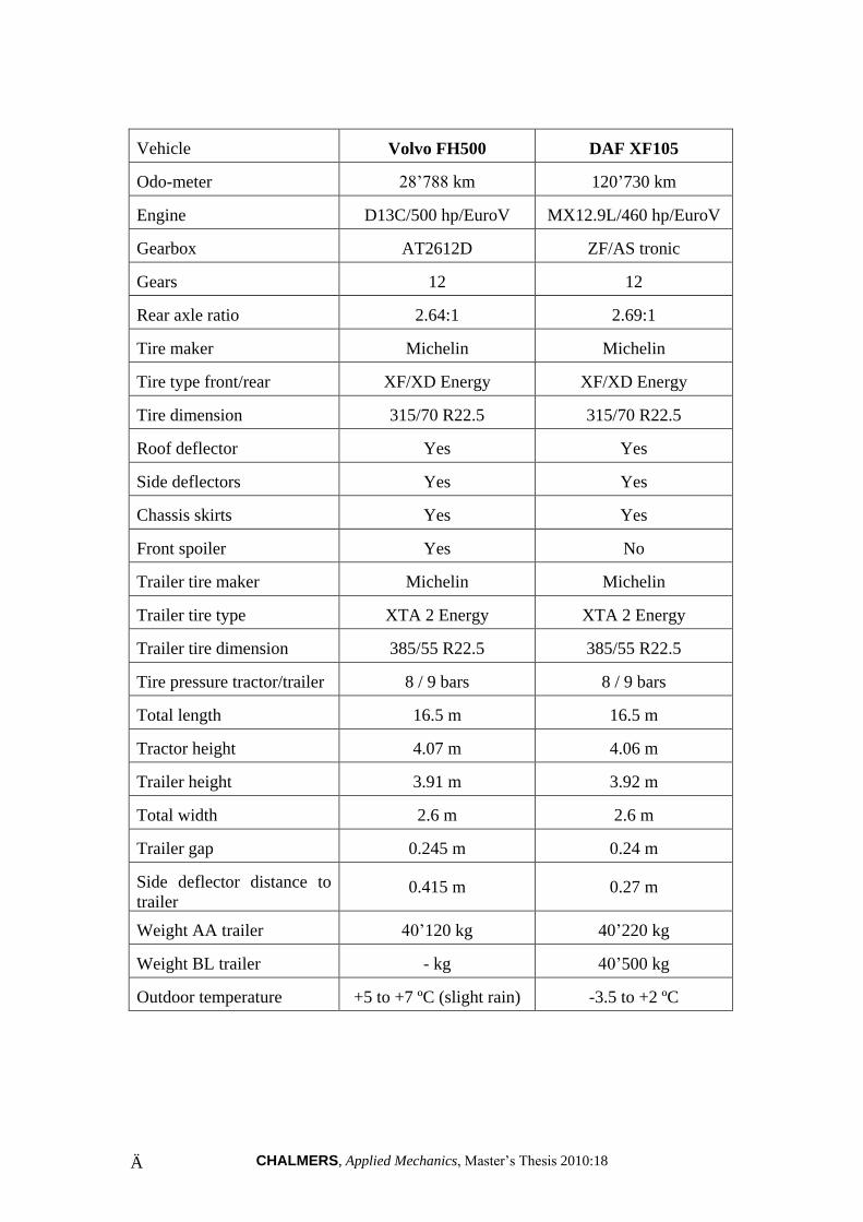
CHALMERS, Applied Mechanics, Master’s Thesis 2010:18 Ä
Vehicle Volvo FH500 DAF XF105
Odo-meter 28’788 km 120’730 km
Engine D13C/500 hp/EuroV MX12.9L/460 hp/EuroV
Gearbox AT2612D ZF/AS tronic
Gears 12 12
Rear axle ratio 2.64:1 2.69:1
Tire maker Michelin Michelin
Tire type front/rear XF/XD Energy XF/XD Energy
Tire dimension 315/70 R22.5 315/70 R22.5
Roof deflector Yes Yes
Side deflectors Yes Yes
Chassis skirts Yes Yes
Front spoiler Yes No
Trailer tire maker Michelin Michelin
Trailer tire type XTA 2 Energy XTA 2 Energy
Trailer tire dimension 385/55 R22.5 385/55 R22.5
Tire pressure tractor/trailer 8 / 9 bars 8 / 9 bars
Total length 16.5 m 16.5 m
Tractor height 4.07 m 4.06 m
Trailer height 3.91 m 3.92 m
Total width 2.6 m 2.6 m
Trailer gap 0.245 m 0.24 m
Side deflector distance to
trailer 0.415 m 0.27 m
Weight AA trailer 40’120 kg 40’220 kg
Weight BL trailer - kg 40’500 kg
Outdoor temperature +5 to +7 ºC (slight rain) -3.5 to +2 ºC
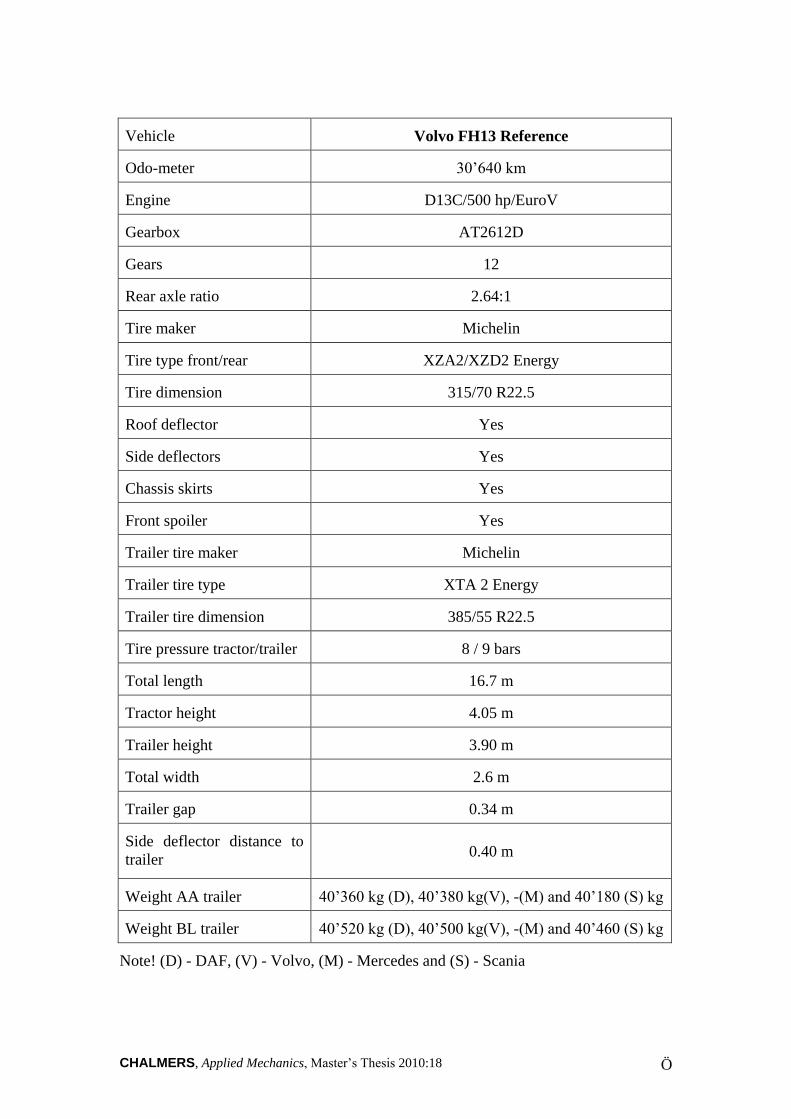
CHALMERS, Applied Mechanics, Master’s Thesis 2010:18 Ö
Vehicle Volvo FH13 Reference
Odo-meter 30’640 km
Engine D13C/500 hp/EuroV
Gearbox AT2612D
Gears 12
Rear axle ratio 2.64:1
Tire maker Michelin
Tire type front/rear XZA2/XZD2 Energy
Tire dimension 315/70 R22.5
Roof deflector Yes
Side deflectors Yes
Chassis skirts Yes
Front spoiler Yes
Trailer tire maker Michelin
Trailer tire type XTA 2 Energy
Trailer tire dimension 385/55 R22.5
Tire pressure tractor/trailer 8 / 9 bars
Total length 16.7 m
Tractor height 4.05 m
Trailer height 3.90 m
Total width 2.6 m
Trailer gap 0.34 m
Side deflector distance to
trailer 0.40 m
Weight AA trailer 40’360 kg (D), 40’380 kg(V), -(M) and 40’180 (S) kg
Weight BL trailer 40’520 kg (D), 40’500 kg(V), -(M) and 40’460 (S) kg
Note! (D) - DAF, (V) - Volvo, (M) - Mercedes and (S) - Scania