DTIC · lynn technical information center, 24001 - 3 copies lynn reports. all classes. 1 copy ... tom scott 34043 d.a. dietrich a-317 d.k. dunbar a-330

AD-A261 227

0 Verification of the Theoretical

Discharge Coefficient of a~ Sub-Critical Flow Meter

by

D.J. Lahti

September, 1990

DTICELEC'TEF _B.11 7 1993

E

Apptoved ~t public 1SDigti~5 1 W

f• 93 2 12 099 93-02773

Aiwrraft Technical Information Series

Title Page

SubjectNumberSUB-CRITICAL R90AEB406

LKHTI, D.J. AIRFLOW METERING Date10/11/90

Title GE Class I_ I Gove..et Ciass U GE Class

VERIFICATION OF THE THEORETICAL II

DISCHARGE COEFFICIENT OF A SUB- GovnmeM CassCRITICAL FLOW METER Unclassified

Copies avilable from Number pagesAircraft Engines Technical Information Center

Lynn 24001 F vendaleN.32 131SummaryII

GEClass II GovernmentClass Unclassified

The objectives of this program were to study the factorsleading to increased errors in sub-critical flowmetering, utilize existing theoretical methods to designa new sub-critical flow meter for very high accuracy,predict its discharge coefficient, and thenexperimentally verify it by calibration with an industrystandard critical flow meter. The meter design wastypical of that used for modern, lightweight, enginemounted bellmouths, but its size was small enough toallow its calibration in a high accuracy laboratoryenvironment. Thus this program provides a "calibration"of the theoretical method and establishes the linkbetween a traceable metering standard and large enginebellmouths whose air flow rates exceed the capacity ofany of the worlds calibration facilities.

"KAe°tetical discharge coefficient, sub-critical airflow

metering, Venturi calibration

Contract Number N/A

SponsoringOrgization AEROTHERMO SYSTEMS INTEGRATION

ApproedbyN/A(Author's Manager)

(Organization)

Oepar 1tn/Operto ADVANCED TECHNOLOGY OPERATION Location Governor's Hill

G1r 71 (6471 FWm.I OV21I7

TECHNICAL INFORMATION SERIES

DISTRIBUTION

EVENDALE TECHNICAL INFORMATION CENTER, N-32 - 6 COPIES EVENDALE REPORTS. ALL CLASSES:1 COPY LYNN REPORTS. CLASSES 1,2. & 3 only

LYNN TECHNICAL INFORMATION CENTER, 24001 - 3 COPIES LYNN REPORTS. ALL CLASSES. 1 COPYEVENDALE REPORTS. CLASSES 1.2, & 3 ONLY.

TECHNICAL INFORMATION CENTER, SCHENECTADY, BLDG. 5 RM 321 - 3 COPIES UNCLASSIFIED CLASS1 THRU 3 ONLY.

RECORDS RETENTION CENTER, LYNN 3109A- MASTER PLUS 5 COPIES. UNCLASSIFIED LYNN CLASS 1 THRU 3REPORTS ONLY

THE DISTRIBUTION OF THIS TECHNICAL INFORMATION SERIES REPORT IS LIMITED TO THE

DISTRIBUTION LISTED BELOW EXCEPT AS APPROVED IN ACCORDANCE WITH THE REQUIREMENTS OF

AEBG 630.10, APPENDIX A.

DISTRIBUTION - LYNN DISTRIBUTION - EVENDALE

Brian Acampa 34022 W.A. Bailey A-317

Dennis Evans 164X9 C. Balan A-330

Tom Scott 34043 D.A. Dietrich A-317

D.K. Dunbar A-330

Accesion For R.G. Keller K-96

NTIS CRA&I A.P. Kuchar A-330DTIC TABUnannounced A. Lingen G-14Justification

B.W. Lord J-40B y .................................................--

Distribution I L.J. McVey A-317

Availability Codes D.W. Rogers H-308SAvail arnd I or

Dis SecalR.E. Russell H-308

(E.J. Stringas G-14

M.W. Thomas K-96

I.W. Victor J-40

GT217 2(5.86)FORWRtYOV217 A

ABSTRACT

Historically, when high accuracy compressible gas flow

measurements are required, flow meters designed for critical

(choked) conditions have been used. Two standard critical

flow meter designs whose discharge coefficients have been

well established are now widely used throughout the world

for such measurements. However in many situations either

critical flow conditions cannot be achieved or these

standard meters cannot be adapted to the physical set up of

the installation where the flow measurements are to be made.

An example of such a situation is the flow metering

bellmouth placed in front of a typical large turbofan engine

on an outdoor test stand. When sub-critical flow conditions

exist measurement errors increase, and when non-standard

meter designs must be used, such as is the case for most

engine bellmouths, their discharge coefficients must be

determined first. When high flow rates exist the only known

way for obtaining the discharge coefficients of non-standard

flow meters is to determine them theoretically.

The objectives of this program were to study the factors

leading to increased errors in sub-critical flow metering,

utilize existing theoretical methods to design a new

sub-critical flow meter for very high accuracy, predict its

discharge coefficient, and then experimentally verify it by

i

calibration with an industry standard critical flow meter.

The meter design was typical of that used for modern,

lightweight, engine mounted bellmouths, but its size was

small enough to allow its calibration in a high accuracy

laboratory environment. Thus this program provides a

"calibration" of the theoretical method and establishes the

link between a traceable metering standard and large engine

bellmouths whose air flow rates exceed the capacity of any

of the worlds calibration facilities. Detailed comparisons

of the theoretical and experimental results are shown and

the effects of uncertainties in the experimental results are

assessed for their impact on discharge coefficient. Finally

recommendations are made for future experimental work that

will further improve our ability to design high accuracy low

pressure loss sub-critical flow meters.

ii

TABLE OF CONTENTS

Pagie

ABSTRACT ................ ................. i

LIST OF FIGURES ............ ............. v

NOMENCLATURE ........ ............... .. ix

Chapter

I. INTRODUCTION AND BACKGROUND. . . . 1

II. STATIC PRESSURE MEASUREMENT ISSUESFOR SUB-CRITICAL FLOW METERS . . . 15

2.1 Introduction ... ......... .. 152.2 Static Pressure Measurement

Accuracy Requirements ..... 172.3 Influence of Static

Pressure Profile ..... 20

2.4 Influence of Static PressureMeasurement Devices ..... 21

III. TEST FACILITY SELECTION CRITERIA . 26

3.1 Calibration Using A StandardCritical Flow Meter ..... 26

3.2 Calibration Using ThroatFlow Field Surveys ..... 27

3.3 Free-Jet Calibration of ThroatPitot-Static Survey Probe . 28

3.4 Capacity For Measurement ofLarge Numbers of StaticPressures ....... 29

IV. METER DESIGN AND PRE-TESTPREDICTIONS .... .......... 31

4.1 Flow Meter Design ...... 314.2 Static Pressure Tap Placement 344.3 Pre-Test Predictions ..... 35

iii

Chapter PAge

V. TEST FACILITY, APPARATUS ANDPROCEDURE ..... ............ 41

5.1 Test Facility .. ........ 415.2 Test Apparatus .......... .. 41

5.2.1 ASME Nozzle ...... 415.2.2 Pitot Static Survey Probe 425.2.3 Flow Meter ...... 425.2.4 Boundary Layer Survey

Probe .. ........ . . 435.3 Test Procedure ... ...... .. 44

5.3.1 Pitot-Static ProbeCalibration ...... 44

5.3.2 Throat Static PressureProfile Surveys . . .. 46

5.3.3 Flow Meter AirflowCalibration ...... 47

5.3.4 Throat Boundary LayerSurveys ...... 47

VI. TEST RESULTS AND DISCUSSION . . . 49

6.1 Pitot-Static PressureProbe Calibration ...... 49

6.2 Meter Throat StaticPressure Surveys . . .. 50

6.3 Measured Discharge Coefficients 536.4 Boundary Layer Surveys . . .. 546.5 Wall Pressure Distributions. 566.6 Charging Station Reference

Pressure .. ......... 57

VII. CONCLUSIONS AND RECOMMENDATIONS. . 60

7.1 Conclusions ... .......... 607.2 Recommendations .. ....... 61

REFERENCES ........ ................ .. 63

TABLE I ................................ 66

FIGURES ............................ . . 68

APPENDIX A - Streamtube Curvature(STC) Method ...... 126

iv

LIST OF FIGURES

FicrurePage

1-a ASME Nozzle Discharge Coefficient Based on0.125-in.Diameter Throat Tap Readings -Compressible flow (air) tests ..... 68

1-b Compressible Flow ASME Nozzle DischargeCoefficients Based on Corrected ThroatTap Readings . . . . ............. 68

2 Isentropic Flow Function ........... .. 69

3 Flow Measurement Error For 1% Error InStatic Pressure Measurement Vs.Mach Number .................. 70

4 Throat Static Pressure Profiles ..... 71

5 Airflow Error Versus Pressure Coefficient. 72

6 Hemispherical Head Static Pressure Probe . 73

7 Typical Meter Throat Static PressureMeasurement Rake Array ........... .. 74

8 Pressure Coefficient Variation ForwardOf Probe Support Cylinder .. ....... 75

9 Typical Non-Standard Nozzle Secondary

Calibration Test Set-Up ....... 76

10 Flow Meter Aerodynamic Contour Definition. 77

11 Flow Meter Theoretical PressureDistribution ... ............. .... 78

12 Flow Meter Theoretical PressureDistribution in Throat Region ..... 79

13 Calculated Skin Friction CoefficientFor Maximum Throat Mach Number ..... 80

14 Predicted Pressure Distributions ..... 81

15 Predicted Throat Displacement Thickness. . 82

v

16 Discharge Coefficient Components ..... 83

17 Predicted Discharge Coefficients ..... 84

18 FluiDyne Channel 12 Static Test Stand. . . 85

19 ASME Nozzle ....... ............... .. 86

20 ASME Nozzle Station Designations ..... 87

21 Pitot-Static Probe .... ............ .. 88

22 Flow Meter ........ ................ .. 89

23 Flow Meter Test Assembly ........... .. 90

24 Pitot-Static Probe Calibration Procedure 91

25 Influence of Calibration Nozzle JetWidth on Calibration Accuracy ...... .. 92

26 Pressure Survey Probe Free JetCalibration Test Results .......... .. 93

27 Predicted And Measured Throat Mach Profiles 94

28 Discharge Coefficient Components ..... 95

29 Throat Wall Average Static Pressure RatioVersus Overall Pressure Ratio ..... 96

30 Survey Probe Effect on Throat WallAverage Static Pressure Ratio, P 5Psw 1.45 97

31 Survey Probe Effect On Throat WallAverage Static Pressure Ratio, P TPSW=1 .28 98

32 Survey Probe Effect On Throat WallAverage Static Pressure Ratio, P TPSW=l.1 99

33 Effect of Survey Probe On MeasuredThroat Static Pressures, r/R=0 ..... .. 100

34 Effect of Survey Probe On MeasuredThroat Static Pressures, r/R=.5 . . .. 101

35 Effect of Survey Probe On MeasuredThroat Static Pressures, r/R=.857. . .. 102

vi

Figuu=r gaae

36 Discharge Coefficient Vs. Wall StaticPressure Ratio . . . . . . . . . . . . . 103

37 Boundary Layer Trip Location . . . . . . . 104

38 Discharge Coefficient Vs. Wall StaticPressure Ratio . . . . . . . . . . . . . 105

39 Measured Boundary Layer At Throat . . . . . 106P T /P Sw 1.1

40 Measured Boundary Layer At Throat . . . . . 107P T /P Sw 1.3

41 Measured Boundary Layer At Throat . . . . . 108P T/PSW = 1.5

42 Measured Boundary Layer At ThroatP T/PSW = 1.3(Effect of Trip) . . . . . .109

43 Predicted Vs. Measured BoundaryLayer Profile P T/PSW = 1-1 . . . . . . . 110

44 Predicted Vs. Measured BoundaryLayer Profile P T /P Sw 1.3 . . . . . . .

45 Predicted Vs. Measured BoundaryLayer Profile P T /P Sw = 1.5 . . . . . . . 112

46 Predicted Vs. Measured BoundaryLayer Profiles P 1.3A/ Psw "(Effect of Trip) . . . . . . . . . 113

47 Throat Displacement Thickness . . . . . . . 114

48 Measured Throat Static Pressures(Data Point 6 and 13) . . . . . . . . . . 115

49 Measured Throat Static Pressures(Data Point 20 and 28) . . . . . . . . . 116

50 Measured Throat Static Pressures(Data Point 38 and 47) . . . . . . . . . 117

51 Predicted Vs. Measured Axial Wall StaticPressure Distributions (Data Point 6and 13) . . . . . . . . . . . . . . . 118

vii

iuareae

52 Predicted Vs. Measured Axial Wall StaticPressure Distributions (Data Point 20and 28) .......... . .............. .... 119

53 Predicted Vs. Measured Axial Wall StaticPressure Distributions (Data Point 38and 47) ......... ................ 120

54 Charging Station Pressure Distortion,Rake 1 ........... ................... 121

55 Charging Station Pressure Distortion,Rake 2 ........ ................... 122

56 Charging Station Pressure Distortion,Rake 3 ................................ .. 123

57 Solution Procedure .... ... ........... 124

58 Finite Difference Stars For Subsonicand Supersonic Flow ..... ........... .. 124

59 STC Streamline/Orthogonal LineSolution Grid ....... .............. .. 125

viii

NOMENCLATURE

SYMBOL DEFINITION

A ...... .. Area, in.2

C ....... ... Curvature, 1/in.

D ........ .. Diameter, in.

CD ....... .. Discharge Coefficient

Cf ...... ... Friction Coefficient

CP . . . . Pressure Coefficient

g. ....... .. Gravitational Constant, ft/sec2

H ........ .. Enthalpy, BTU/Ibm

M ........ .. Mach Number

P ........ .. Pressure, lb/in 2

r,R ........ Radius, in.

...... Gas Constant, (ft-lbf)/(lbm- R)

Re ..... .. Reynolds Number, PVD

S ........ .. Entropy, BTU/lbm

T......... Temperature, R

u ........ ... Axial Velocity

v,V ..... .... Normal, Total Velocity, ft/sec

W ........ ... Weight Flow, lb/sec

X ........ .. Axial Distance

y ........ .. Vertical Distance

iX

SYMQ DEF!ITIO

....... Ratio of Specific Heats

........ .. Boundary Layer Thickness, in.

* ...... .. Displacement Thickness, in.

........ .. Momentum Thickness, in.

....... Viscosity, lb-sec/ft 2

P .. ... .. Density, lbm/ft 3

....... Velocity Potential

....... Stream Function

amb. . . . . Ambient

id ..... Ideal

j ..... Jet

1 ..... Local

O,T ..... Stagnation, Total Conditions

S ..... Static

SW ..... .. Wall Static

1-D ........ One-dimensional

x

Chapter I

INTRODUCTION AND BACKGROUND

For most engineering purposes the measurement of physical

phenomena is based on an accepted standard. Unfortunately

the measurement of fluid flow has no exact standard of

extremely high accuracy such as is possible with length,

time, mass, pressure, temperature and many others. This is

particularly true when the flow rates are very large.

Although it is possible to measure time accurately and also

density, which is the correlation between volume flow and

weight flow, the accurate measurement of large weight or

volume is difficult (Reference 1). It is difficult and

expensive to attempt to operate large weigh tanks or volume

tanks in other than a laboratory specifically designed for

the measurement of fluid flow. Although there are several

facilities in existence for the direct, or primary

measurement of relatively small quantities of fluid flow,

there are only a handful in existence capable of measuring

large quantities of fluid flow. In addition, this is only

true for cases where the fluid is a liquid. Because of the

low density of gases compared to liquids, the direct

measurement of large quantities of gas flow is not possible,

and to this author's knowledge there are only four

facilities in the free world (Reference 2) where the direct,

primary measurement of small quantities of gas flow is

-1--

performed. The largest flowrate any of these facilities is

capable of measuring is about 10 pounds per second.

Primary methods of flow measurement, by definition, are

accomplished without calibrations by other flow measurement

devices. So called secondary methods require calibrations

which serve as corrections that are applied as discharge

coefficients in calculating the flow rate. Since some

accuracy is lost each time a calibration is transferred from

one flowmeter to another, it is desirable to minimize the

number of calibration steps between the primary method and

the flow measurement that is required. As Arnberg, et al,

(Reference 3) point out it would be desirable to obtain the

required measurement directly by means of a primary method,

so that no calibration transfers would be needed. However,

as they note there are two limitations to this ideal in

practice. First, all primary methods do not have the same

accuracy. Since there is nothing that requires high

accuracy in a primary method, it is possible that a

secondary measurement based on a primary calibration of high

accuracy could be more accurate than a measurement obtained

directly by a primary method of poor accuracy. Second,

since most primary methods of gas flow measurement lack

flexibility when designed for the highest possible accuracy,

they are often incompatible with the installation

circumstances of the particular flow measurement needed.

-2-

Therefore in the case of compressible gas flow measurement

there has evolved over the past thirty years two accepted

standard flow meter designs that represent an "optimum"

compromise between the high accuracy obtainable by the best

primary calibration methods and the flexibility of secondary

methods with a minimum loss of accuracy due to calibration

transfer. These standard flow meters are the Smith and Matz

critical flow circular-arc throat venturi and the ASME

critical flow nozzle.

Both Smith and Matz (References 4, 5) and Stratford

(Reference 6) discussed many of the advantages of metering

airflow using critical flow circular arc venturis. In their

pioneering work to demonstrate the advantages of choked flow

metering Smith and Matz (Reference 5) argued that metering

at conditions where the Mach numbers across the meter throat

were at or near unity provided a situation where errors in

calculated flow rate due to pressure measurement errors

would be minimized. They stated that "at critical flow

conditions an error in total pressure of +0.25 percent

results in an airflow rate error of only ± 0.25 percent, and

no additional error contribution results from the static

pressure measurement. At critical flow conditions the

throat static pressure is constant and, what is much more

important, need not be measured at all because it can be

calculated from consideration of the properties of the

-3-

flowing gas. They go on to state "For a given accuracy of

pressure measurement then, the error in f low rate at Mach

number 0. 3 is, for the case where errors are additive, 15

times as great as the error at the critical flow rate."

They go on to discuss the factors which lead to the

selection of a suitable venturi contour for metering flow at

critical conditions. It is interesting to note that one of

them relates to the contour being of a simple enough

geometric shape that its flow field could be calculated on a

theoretical basis. At the time that their work was done

(Circa 1958-1963) the most relied upon method for the

calculation of the transonic flow field in a nozzle throat

was that due to Oswatitsch and Rothstein (Reference 7). It

was an approximate method for the solution to the velocity

potential equation utilizing series expansions for the axial

and radial velocity components and simple analytical

expressions for the wall geometry. The method was only

valid in the immediate vicinity of the nozzle throat where

the wall slopes were small. The turbulent boundary layers

were calculated utilizing Tucker's (Reference 8) approximate

method. They argued that in spite of the limitations of

these theoretical methods, when operating at critical flow

conditions predictions of the discharge coefficient were

accurate to within ±0.25 percent for their recommended

circular arc throat contour which was blended into a conical

exhaust diffuser. They then built and tested their

-4-

recommended venturi design. In order to experimentally

determine the discharge coefficient of the meter it was

built large enough (5.64 inch throat diameter) to allow

fundamental measurements of the throat static pressure

profile and wall boundary layer thickness. Thus, in

principle, they "calibrated" the flow meter using a

theoretical prediction and verified that the predictions

were valid to within a certain accuracy. Their results

showed that their predictions of discharge coefficient were

within approximately 0.05 percent of the experimental values

over the range of Reynold's numbers of the tests. On the

basis of this work their recommended circular arc venturi

has become an industry standard design and is now used in

test facilities throughout the world.

Stratford (Reference 6) argued along similar grounds that

the most accurate gas flow meter is a circular arc throat

contour operating at critical conditions. His recommended

throat contour was only slightly larger than that of Smith

and Matz on the grounds that the larger throat wall radius

of curvature reduces the radial pressure profile in the

throat and thus minimizes the error in predicted discharge

coefficient due to inadequacies in the then available

transonic flow field predictions.

-5-

The origin of the critical flow ASME nozzle is not as clear

as that of the Smith and Matz circular arc venturi. Its use

as a critical flow meter appears to have evolved over time

from its use as a liquid only flow meter. It was originally

promoted by the Instruments and Apparatus for the

Measurement of Fluid Flow Subcommittee of the ASME Power

Test Codes Committee circa 1934. Its discharge coefficient

has been well established for incompressible fluids

(Reference 9) in primary (direct-weigh) calibration

facilities. The normal practice has been to apply the

results from such calibrations with incompressible fluids

directly to the compressible measurement problems by appeal

to the laws governing dynamic similarity of the flows. This

appeal to similarity is made at constant values of Reynolds

number based on the throat diameter with some Mach number

constraints. The one recommendation by the ASME (Reference

9) is that this method can be used as long as the throat

Mach number is less than 0.95. Smith and Matz (Reference

10) conducted an exhaustive and systematic search of U.S.

and foreign technical journals and other archive documents

and found no evidence of reports of systematic experiments

to determine quantitatively the tolerances involved in this

appeal by the ASME to dynamic similarity between

compressible and incompressible flows, at least in the size

range of throat diameters greater than several inches.

-6-

To this author's knowledge the only known experimental work

to establish the discharge coefficient of critical flow ASME

nozzles was performed by Holdhusen and Peruse (Reference

11). In these tests the meter exit boundary layer profiles

were measured and the resulting mass and momentum deficits

were used to compute the discharge and thrust coefficients

respectively. Since the meter was always choked and its

throat section is cylindrical, Holdhusen and Peruse argued

that the influence of a non-uniform radial pressure profile

is negligible. In the test meter they placed static

pressure taps along the throat wall to verify this argument.

Although the flow was not surveyed across the throat, the

wall taps would indicate the maximum influence of a

non-uniform radial profile since the highest velocity occurs

there. Their static pressure measurements confirmed their

belief. They showed that the maximum effect of a

non-uniform radial velocity profile to have less than a 0.1%

impact on discharge coefficient. Although this work was not

widely published it was significant because it proved for

critical flow conditions only the effect of the throat

boundary layer blockage need be accounted for in determining

ASME nozzle discharge coefficients. Over the past twenty

five years this work gradually received wide scale

acceptance and thus critical flow ASME nozzles are also

widely used in test facilities throughout the world.

-7-

Although it is desirable to utilize critical flow meters

whenever possible because of their inherent accuracy

"advantage" it is often not possible. In many industrial

applications it is necessary to accurately measure the air

flow in devices not capable of generating the pressure

differential necessary to produce critical conditions in the

meter throat. There are also situations where choked flow

could be produced in the meter throat, but other factors

prevent the use of a critical flow meter. Situations where

the available space prevents the use of a standard

circular-arc venturi with its relatively long supersonic

diffuser can dictate the use of a much shorter non-standard

meter design. If there is a requirement that the discharge

pressure loss and/or distortion be kept to a minimum,

critical flow meters could not be used because of their

inherently high pressure loss and distortion associated with

the shock system and boundary layer separation in the

supersonic diffuser. Coupled with the fact that there are

no facilities (either primary or secondary) capable of

calibrating compressible gas meters where the flowrates

exceed approximately 300 pounds rer second it is clear that

there is a need for a procedure to "calibrate" non-standard

subcritical flow meters having high flow rates.

In the absence of facilities for calibrating such

non-standard sub-critical flow meters the industry has

-8-

resorted to a variety of methods for filling this void. The

most worthy attempts have been based in some way on the use

of theoretical methods; however, to this day no systematic

procedure has emerged as being the accepted best. In

addition, most such attempts go undocumented and are not

reported in the open literature. Although there have been

several successful attempts at the theoretical prediction of

the discharge coefficient of critical flow meters since the

work of Smith and Matz as discussed previously, only one

such case has been found in the open literature for

sub-critical flow meters. This work was also performed by

Smith and Matz (Reference 10) approximately ten years after

their work on circular-arc critical flow venturis.

This work was motivated by the question of whether the

discharge coefficient established for a nozzle from an

incompressible calibration using water would be the same as

that obtained for the nozzle using a compressible gas at the

same Reynolds number but at sub-critical throat Mach

numbers.

They conducted an elaborate program consisting of

calibrations of an 8 inch throat diameter ASME nozzle using

both water and air. The water calibrations were performed

using the primary method of direct weighing of the water.

The air calibrations were performed using a 5.64 inch

-9-

diameter circular-arc critical flow venturi whose discharge

coefficient had been determined using the theoretical

procedure they had established approximately 10 years

earlier as discussed previously.

Both the water and air calibrations were conducted with

identical pressure instrumentation in the ASME nozzle to

minimize differences in discharge coefficient due to

differences in the instrumentation itself. In addition to

the instrumentation necessary for discharge coefficient

determination, a large amount of diagnostic instrumentation

was included to ascertain the details of the flow fields

upstream of the nozzle entrance as well as throughout the

nozzle itself.

As mentioned previously theoretical predictions of the ASME

nozzle compressible flow field were also made in support of

this extensive test program. These calculations were made

in order to compare with the diagnostic flow field

measurements to aid in understanding and interpreting the

discharge coefficient results. Although details of the

computer code were not discussed in their paper, the

following general description about it was given. "The

Wehofer-Moger transonic flow computer program employs a

direct numerical integration of the differential equations

for continuity, radial momentum, axial momentum, and energy

-10-

posed in the unsteady or time-dependent form. The gas

involved is assumed to be inviscid, adiabatic, and thermally

perfect."

The application of this computer code to the ASME low beta

ratio nozzle is the first (and only) known such work on an

unchoked compressible gas metering standard that has been

published in the open literature.

Their compressible flow calibrations of the ASME nozzle were

conducted over a range of throat Mach numbers from 0.4 to

1.0. The incompressible flow (water) calibrations were

conducted over the same range of throat Reynolds numbers as

for the compressible calibrations. Theoretical flow field

solutions were conducted for the same conditions as for the

compressible flow calibrations.

Figures la and lb show the results of the compressible flow

calibrations obtained by Smith and Matz. These two figures

are taken directly from their paper (Reference 10). The

upper figure (la) shows the discharge coefficients obtained

for three values of throat Mach number based on the ASME

recommended static pressure tap size and placement. Smith

and Matz noted that some of the coefficients were greater

than unity and there was large scatter in the data,

particularly for throat Mach numbers less than 1.0.

-11-

In comparing their theoretical solutions with their static

pressure survey data at the meter throat they noted good

agreement in both pressure level and profile except at the

wall (where the measured pressures were obtained from the

ASME recommenled 0.125 inch diameter taps as opposed to

their survey probe). As a result of this observation they

corrected the measured wall pressure data based on the

results of an experimental study by Rayle (Reference 12)

which showed the effect of tap size on indicated pressure.

This corrected data is shown in the lower plot Figure lb.

Clearly the correction reduced the scatter in the discharge

coefficient for the unchoked Mach numbers, but it is still

nearly twice as large (± 0.5 percent) as the critical flow

data shown.

Smith and Matz draw several important conclusions from this

work. First they determined that the ASME recommended

discharge coefficients based on incompressible water tests

could not be uscd for compressible gases. At the lowest

throat Mach number of 0.4 the water results differed from

the compressible results by more than one percent.

Their final conclusion was stated as follows: "A precise

theoretical model of the complex flow field for both

subsonic and critical-fiow conditions in the ASME long

radius low beta ratio nozzle has been developed and has been

-12-

verified by comparison with experimental data. Use of this

powerful analytical tool should provide a means for an

improved correlation of experimental measurements of nozzle

discharge coefficient." Unfortunately they did rot show

comparisons of predicted discharge coefficients versus their

measurements, and they did not make detailed boundary layer

measurements which might have provided a better understand-

ing of the source of the large data scatter. It is also

unfortunate that although their work was conducted nearly

thirty years ago there have been virtually no published

works since then which attempt to build upon their

experience and the suggested insight that the improved

theo-etical methods could provide. The partial success of

Smith and Matz and other successes in the use of CFD since

then, along with the continued push for increased flow

metering accuracy in sub-critical flow environments, led to

the idea that a comprehensive experimental program was still

needed to provide a highly accurate sub-critical flow meter

design that did not have many of the limitations of unchoked

ASME metering nozzles.

Therefore the main objective of this program was to

experimentally verify the accuracy of a theoretical method

for determining the discharge coefficient of a sub-critical

flowmeter of non-standard design to an accuracy comparable

-13-

to that of standard critical flow venturis, which is +0.25

percent. The rationale for this was that once the method

had been verified it could be utilized on any sub-critical

flow meter independent of its size, and in particular very

large flow meters where there are no other means available

for establishing their discharge coefficients.

A second objective was to establish a new sub-critical

compressible flow metering standard to replace the ASME low

beta ratio nozzle which has many inherent problems when used

for unchoked flows. To this author's knowledge a program

such as this has never been conducted. It was intended that

the data obtained could also be used by others to serve as a

benchmark for establishing the accuracy of other theoretical

methods that presently exist or will be developed in the

future. The program formulated to accomplish this is

described below. It represented a blending of existing

theoretical methods with established critical flow metering

standards and procedures.

-14-

Chapter II

STATIC PRESSURE MEASUREMENT ISSUES

FOR SUB-CRITICAL FLOW METERS

2.1 INTRODUCTION:

A head type flow meter produces a constriction in the gas

stream that causes a pressure differential which is a

function of the flow rate through it. The higher the flow

rate the higher the pressure differential.

The discharge coefficient of a head type flow meter is

defined as the ratio of the actual flow rate to the ideal

one-dimensional inviscid flow rate that would exist if all

the flow were at the velocity corresponding to the static

pressure at the meter throat wall. The more uniform the

velocity profile across the throat of the meter the higher

its discharge coefficient. A discharge coefficient of unity

would imply a perfectly uniform velocity profile and no wall

boundary layer. Thus the accurate determination of the

discharge coefficient of a flow meter is dependent on three

primary factors. The first is the velocity level that

exists at the throat of the meter, the second is the profile

of velocity (pressure) across the meter throat and the third

is the thickness of the throat wall boundary layer.

-15-

There are four methods for determining the discharge

coefficient of a head type flow meter. The first is to

survey the velocity, pressure and temperature fields across

the meter throat to determine the PV profile which can then

be integrated to determine the actual mass flow rate. The

second is to compute these same quantities using a

theoretical method and then performing the same integration

of the PV profile. The third is to physically weigh the

quantity of fluid that is passed through the meter in a

given amount of time. This is called a primary calibration

because the actual mass is measured directly. The fourth is

to calibrate the flow meter using another flow meter whose

discharge coefficient is already known. This type of

calibration is called a secondary method because the actual

mass flow through the meter is not measured directly, but

rather it is calculated using the known discharge

coefficient of another flow meter.

As discussed in Chapter I the determination of discharge

coefficients of compressible gas meters using primary

calibration methods is limited to flow rates of

approximately 10 pounds per second. Secondary methods have

been used to determine compressible gas meter discharge

coefficients for flow rates up to approximately 300 pounds

per second. Thus the only methods available for determining

meter discharge coefficients at flow rates exceeding about

-16-

300 pounds per second involve either measuring the throat

pressure profile or calculating it using a theoretical

method.

Since the purpose of this program was to verify the accuracy

of the theoretical method for determining discharge

coefficient it involved both the calculation of the throat

pressure profiles and then comparing them to the measured

profiles of a specific flow meter design. Before proceeding

to a discussion of the flow meter design itself it is

important to discuss the issues relating to static pressure

measurement that will influence the design of any

sub-critical flow meter.

2.2 STATIC PRESSURE MEASUREMENT ACCURACY REQUIREMENTS

As discussed in Chapter I, when mass flow is to be measured

when sub-critical flow conditions exist, it becomes

necessary to accurately determine the static pressure field

across the meter throat. Although in principle this is

simple, in practice it is an extremely difficult task and in

fact, it is because of this difficulty there are no known

standard subcritical flow meters in existence today with

accuracies that match those of critical flow meters.

-17-

The importance of accurate static pressure measurement in

the throat of an unchoked flow meter is illustrated with the

aid of Figures 2 and 3. The isentropic flow function

fETI" I also called Fliegner's Formula, (Reference 13), isPO A

given by

IPVVFTO S ly, S= (T

(A)YYP. A 0 Jý(Y- 1) PO

where w/A is the weight f low per unit area, To and Po are

the stagnation temperature and pressure respectively and PS

is the static pressure. In Figure 2 the isentropic flow

function is plotted as a function of the static-to-total

pressure ratio P S /P 0*

As one moves away f rom unity Mach number in either the

subsonic or supersonic direction, the slope of the

isentropic f low function curve becomes increasingly steep.

Thus errors in the measurement of static pressure will have

an increasingly larger effect on the weight flow error the

further away from unity Mach number. If the flow function

equation is differentiated with respect to pressure ratio,

P S /PO, one obtains

d WFTOPO A KCr,+T2

d( P S)PO

where K = R_ -^g)R(y -I)

I -^f -; F

TQ II1 ( 4- (S\

and

T22y ( [l-10S)T]

This equation can now be used to compute the error in weight

flow W as a function of the pressure ratio. This is shown

in Figure 3 where the error in weight flow rate due to an

error in static pressure (Ps) of 1% is plotted as a function

of Mach number. This curve illustrates why critical (sonic)

flow meters are used whenever possible. It also shows that

if one is to achieve flow measurement accuracy within 1% at

a meter throat Mach number less than approximately 0.65, the

static pressure must be measured with an error of less than

1%. The pressure measurement accuracy requirement increases

rapidly as throat Mach number decreases. For example, at a

throat Mach number of 0.1 a static pressure measurement

error of 1% would produce a flow measurement error of

approximately 60%.

-19-

2.3 INFLUENCE OF STATIC PRESSURE PROFILE

In order to determine the discharge coefficient of any flow

metering device, an accounting of the throat static pressure

profile must be taken. In a critical flow meter the profile

is only dependent on the meter geometry (excluding the minor

secondary influence of the meter wall boundary layer)

whereas the profile in an unchoked meter is not only

dependent on the meter geometry, but also ironically on the

flow rate itself. As the flow rate through the meter is

decreased, the radial variation of the static pressure

decreases and the absolute level of pressure increases.

Thus, although the v in pressure across the meter

throat is reduced, because the Mach number is also

decreasing, the sensitivity to measurement error is

increasing and the need to measure the profile more

accurately increases. This is illustrated in Figure 4,

where the radial profiles of static-to-total pressure ratio

were calculated using the method of Reference 14 for a

typical large jet engine bellmouth for a range of specific

flows represented by the indicated average Mach numbers.

The dashed lines on either side of each profile show the

range of pressure ratio variation representative of a ± 0.5%

flow rate variation. At the lowest average Mach number

shown, the ± 0.5% variation band is very small even though

-20-

the difrenc between the wall value and centerline value

is less than half of the difference at the highest average

Mach number.

2.4 INFLUENCE OF STATIC PRESSURE MEASUREMENT DEVICES

The difficulties associated with measurement of the throat

radial static pressure profile is the major factor which

prevents subcritical flow meters from being used more widely

for high accuracy meters. The main reason for this

difficulty is that the devices used to measure static

pressure disturb the flow field being measured, thus

altering the local pressure at the point of measurement.

Figure 5 shows the error in airflow that would result from

the disturbance to the local pressure (as indicated by

pressure coefficient, Cp)

P -Pwhere Cp S I

21

and P1 and N1 are the true local undisturbed pressure and

Mach number respectively, and Ps is the sensed pressure

caused by the placement of the measurement device in the

local flow field. As indicated in this figure the pressure

coefficients for a minimum error of 0.25% are very small.

At a true undisturbed Mach number of 0.7 the pressure

coefficient on the static probe must be less than 0.01. At

an ambient pressure of 14.7 psia this means a true pressure

-21-

disturbance of less than 0.05 psia. At a true Mach number

of 0.2 the pressure coefficient would have to be less than

.005, which means an absolute pressure disturbance of less

than 0.0021 psia.

This problem is further illustrated in Figures 6 and 7.

Figure 6 shows a typical static pressure probe design which

consists of a cylindrical tube with a hemispherical head.

The four static pressure ports are usually located some

distance (X) aft of the nose leading edge. Shown beneath

the probe are its characteristic pressure distributions

(Reference 15) for a range of free stream Mach numbers. It

is seen that for all subsonic flow along the probe the

effect of this nose geometry is to depress the pressure

below the local ambient pressure for about 4 probe

diameters. As the freestream Mach number is increased (but

still remains subsonic), such that local supersonic flow

exists at the cylindrical portion, the shock wave formed

causes the pressure at the sensing ports to be higher than

the local ambient. Although many other static probe head

designs have been utilized over the years (Reference 16),

they all require the placement of the sensing ports a

significant distance downstream of the leading edge in order

to be out of the influence of the nose pressure field.

Often for very large sub-critical flow meters these static

probes are mounted in a radial array on a fixed structure

-22-

that either spans the throat of the meter or is centilevered

from one wall. Depending upon the anticipated

circumferential non-uniformity of the static pressure field

to be measured, there can be as many as eight of these

"rakes" or as few as one. Typically each of these rakes

would have up to 8 static probes, thus providing for as many

as 64 individual static pressure measurement locations

within the throat.

Since the radial structural struts that support the

individual probes must be rigid enough to accurately

maintain the probe positions under their aerodynamic

loading, they are significantly larger than the probes

themselves. Depending upon the aerodynamic environment

(pressure level, temperature, and Mach number) in which they

will be located, they may have a wide variety of

cross-sectional shapes ranging from circular to

airfoil-like. A typical cross section for relatively low

Mach numbers would have a hemispherical leading edge with

parallel side walls and a hemispherical trailing edge as

shown in Section A-A of Figure 7 along with a typical static

probe array. Since the static pressure sensing ports of the

probe are in front of the relatively blunt support strut,

they must be placed far enough forward of the strut to be

out of the influence of its leading edge stagnation region.

Krause (Reference 17) conducted an experimental study to riap

-23-

the stagnation region in front of support struts having a

cylindrical cross section. A summary of those results are

shown in Figure 8. It is seen that the pressure ports must

be placed at least 12 to 15 diameters forward of the support

strut to be sensibly removed from its influence. These

results, along with those of Reference 15 show that the

placement of the pressure ports far enough aft of the probe

leading edge influence and far enough forward of the support

strut leading edge influence is a critical factor in

achieving a high level of accuracy in static pressure

measurement. Usually aerodynamic interference and

measurement accuracy are not the only factors considered in

determining the placement of the static pressure ports.

Structural design considerations as well as the physical

blockage of the rake are also important. As mentioned

previously, it is desirable to place the pressure ports at

least 12 to 15 support strut thicknesses forward of the

strut leading edge. However, the structural stiffness of

the cantilevered probe on the cantilevered strut is often

not sufficient to allow the pressure port placement that far

forward without significant vibration or divergence

problems. Under these circumstances the pressure ports are

located within either the influence of the probe tip or the

strut leading edge, or both. When this is the case the

influence of the probe/strut combination is usually unknown

-24-

and the rake must be calibrated. That is the rake with its

unique placement of the static pressure sensing ports and

its unique aerodynamic geometry must be placed in an

aerodynamic flow field whose local static pressure and Mach

number are known a-priori and the sensed pressure and Mach

number can be calibrated to these known values.

-25-

CHAPTER III

TEST FACILITY SELECTION CRITERIA

3.1 CALIBRATION USING A STANDARD CRITICAL FLOW METER

In order to verify a procedure to theoretically determine

sub-critical flow meter discharge coefficients to the level

of accuracy that matches that of critical flow meters, it

was felt that the program must include the use of one of the

two accepted critical flow metering standard nozzles.

Either the Smith and Matz circular-arc venturi (Reference 4)

or the ASME low beta ratio nozzle (Reference 9) was

considered acceptable. Thus the chosen critical flow meter

whose discharge coefficient is already known would be used

as the transfer standard to perform a secondary calibration

of the non-standard sub-critical flow meter designed for

this program.

Figure 9 shows a typical test set up that would be used for

such a calibration. In this arrangement the non-standard

flow meter is connected in series with the standard critical

flow meter whose discharge coefficient is known. As

discussed in Section 2.1 the discharge coefficient of the

non-standard nozzle is defined as the ratio of the actual

mass flow to the ideal one-dimensional inviscid flow that

-26-

would be passed by the nozzle if all the flow were at the

velocity corresponding to the wall static pressure and the

upstream total pressure and temperature. Therefore for each

flow rate through the system the actual flow is determined

from the calibrated upstream critical flow metering nozzle

and the ideal one-dimensional flow is calculated from the

measured tot i pressure (PT), total temperature (TT), throat

wall static pressure (PSw), and throat area A in the

non-standard nozzle.

The issue of greatest importance with respect to the test

facility selection for this purpose is that it had to have

the capability and demonstrated experience to conduct such

tests to the levels of accuracy and precision required. The

final assessment of the success or failure of the

theoretical procedure to predict the discharge coefficient

of the non-standard sub-critical flow meter design would be

based on how well the theoretical predictions compared with

the discharge coefficients established from these secordary

calibrations.

3.2 CALIBRATION USING THROAT FLOW FIELD SURVEYS

As discussed in Section 2.1 another method for determining

the discharge coefficient of a non-standard flow meter is to

survey the throat pressure and temperature profiles from

-27-

which the PV profile can be calculated and then integrated

to establish the actual flow rate. Although this method is

the least accurate of the three known methods for

determining sub-critical flow meter discharge coefficients

as discussed in Section 2.3 and 2.4, it was considered to be

an important secondary, or back-up requirement in selecting

the test facility. Such back-up measurements provide a

means for reconciling the observed discharge coefficients

obtained from the critical flow meter with the observed

throat flow field measurements and thus serve as an

important diagnostic tool. Therefore the facility selected

had to have a large enough airflow delivery capacity to

allow a meter physical size large enough to permit throat

static pressure surveys and wall boundary layer surveys over

the full range of throat Mach numbers planned.

3.3 FREE-JET CALIBRATION OF THROAT PITOT-STATIC

SURVEY PROBE

As a consequence of the intention to determine the meter

discharge coefficient from throat static pressure profile

surveys a third factor considered in selecting the test

facility was the requirement for conducting free-jet

calibrations of the pitot-static probe to be used in the

surveys. As discussed in Section 2.4 it is imperative that

whenever a particular static pressure measuring device is to

-28-

be used for high accuracy testing, it must be calibrated in

a known flow field. Therefore the test facility had to have

the capability to conduct a high accuracy free-jet

calibration where the jet size was commensurate with that of

the meter throat where the pressure profile surveys were to

be taken.

3.4 CAPACITY FOR MEASUREMENT OF LARGE NUMBERS

OF STATIC PRESSURES

Finally the last significant factor in the test facility

selection was the capability for making a large number of

accurate wall static pressure measurements throughout the

meter. The rationale for this requirement was to provide

enough detailed flow field measurements throughout the meter

for detailed and extensive comparisons with the theoretical

predictions which were to be performed. These static

pressure measurements were also intended to provide a data

base for others wanting to validate their own theoretical

methods.

The facility selected for conducting the tests was FluiDyne

Engineering Corporation in Minneapolis, Minnesota. The test

facilities at their Medicine Lake Aerodynamic Laboratory

were ideally suited for the planned tests. This facility

-29-

has a number of test channels which are normally used for

scale model exhaust nozzle testing. The model size finally

selected was chosen such that existing facility adapter

hardware could be used. A detailed description of the test

set up and procedure is provided in Chapter V.

-30-

CHAPTER IV

MUTER DESIGN AND PRE-TEST PREDICTIONS

4.1 FLOW METER DESIGN

The meter design was developed in conjunction with the

facility selection, the intended future use of the

sub-critical flow metering procedure specifically for large

engine flow rate determination, and the verification of the

metering procedure using an existing critical flow metering

standard.

The flow meter aerodynamic contour definition is shown in

Figure 10. Figure 11 shows the aerodynamic contour along

with the theoretically predicted wall pressure distribution

using the STC inviscid computer code. The meter design will

be discussed with reference to these two figures. In Figure

10 it is seen that the meter consists of four main segments.

The upstream contracting section has an elliptical contour

from the so called "hilite" station (X = 0, R = 4.8785).

The upstream 6.125 inch radius pipe is part of the facility

adapter hardware. A radial line connects the two at station

0. The throat region of the meter consists of a 1.827 inch

cylindrical section from the end of the elliptical section

to the start of the diffuser.

-31-

The throat radius is chosen based on a compromise between

two conflicting requirements. Since it is desirable to

operate the meter over a wide range of flow rates, the

throat should be kept as small as possible in order that the

Mach number be as high as possible to minimize the effect of

pressure measurement error at the lowest anticipated flow.

However since the meter is intended to be used in front of a

jet engine, the throat must be large enough so as not to

cause choking at the highest anticipated flow. In addition,

the diffuser area ratio must be small enough, and its

contour gradual enough to prevent boundary layer separation

which would generate undesirable pressure distortion at the

engine face.

The cylindrical section which connects the upstream

contraction with the downstream diffuser is intended to

provide a region of constant physical flow area for ease of

area measurement. Since the absolute flow rate through any

meter depends on its actual throat area, and one's ability

to measure it, a cylindrical section is chosen to minimize

the area measurement uncertainties. Although this may not

be a critical problem for small meters whose contour can be

inspected with great accuracy on modern contour measuring

machines, it is a problem on very large meters whose size

prohibits this possibility. The length of the cylindrical

section is determined in an iterative procedure which

-32-

involves theoretical solutions such as shown in Figure 11.

This figure shows that there are two localized overacceler-

ations at the curvature discontinuities that occur at each

end of the cylinder between the end of the contracting

section and the start of the diffusing section. Between

these two locations it is seen that there is a relatively

flat region in the pressure distribution. This pressure

"flat" is highly desirable from an experimental error point

of view. When seeking to determine the axial location of

the throat wall static pressure taps, small errors in their

placement in the meter are minimized since the pressure in

this region is changing slowly. Thus to determine the

length of the cylindrical section for a given flow meter,

the theoretical solution for each assumed length is examined

to find one having a pressure flat that is long enough to

accommodate the expected static pressure tap location

uncertainty. Figure 12 shows an expanded view of the

calculated pressure distribution in this region for the

selected meter design at the nominal throat Mach number of

0.767. The variation in pressure distribution is such that

an error in pressure tap placement of approximately a half

inch would cause no more than about a 0.25% flow error.

In order to ascertain that the diffuser would remain separ-

ation free over the complete flow range of the meter, a

boundary layer solution was conducted using the pressure

-33-

distribution from an STC solution at the highest antici-

pated flow rate. Since the steepest adverse pressure

gradient in a diffuser occurs at the highest throat Mach

number (flow rate), if it does not separate at this

condition it will remain separation free at all lower Mach

numbers. Figure 13 shows the computed skin friction

coefficient for the case of the maximum nominal throat Mach

number of 0.767. The skin friction coefficient remains well

above a value of 0.001 throughout the diffuser.

4.2 STATIC PRESSURE TAP PLACEMENT

The pressure distribution in Figure 11 was used to determine

where the static taps should be placed throughout the model.

Since one of the purposes of this program was to prcvide a

data base for establishing how well current theoretical

methods could predict such subsonic flowfields the model was

very heavily instrumented. A total of eighty static

pressure taps were installed along the wall of the meter.

In addition to providing a detailed description of the axial

pressure distribution for comparison with the theoretical

predictions, at some axial stations taps were placed at

several circumferential locations for use in assessing the

uniformity of the flow in the model. There were 8 taps

placed every 45 degrees around the circumference of the

throat metering plane at X - 4.031. These 8 taps were to be

-34-

used to provide the basic wall static pressure reading as

the means for measuring the actual airflow through the meter

in conjunction with the theoretically determined discharge

coefficient.

In addition to providing detailed static pressure data along

the meter wall, it was planned that throat static pressure

surveys also would be obtained. Therefore a pitot static

probe was designed using the static port placement criteria

of Reference 17 and shown in Figures 6 and 8. Since the

profiles were to be obtained at the throat metering plane

(station 4.031) the probe tip extends upstream of this

location by 4 probe diameters in order that its influence

not be felt at the static ports which are located at X =

4.031. Similarly the aft support rod is downstream of X =

4.031 by 12 diameters to remove its upstream influence.

Details of the model hardware and instrumentation are

discussed in Chapter V.

4.3 PRE-TEST PREDICTIONS

During this program the meter design was accomplished in

conjunction with the aerodynamic performance and flow field

predictions because of the iterative nature of the process.

The previous section discussed meter design issues. This

section will discuss the meter aerodynamic flowfield and

-35-

discharge coefficient prediction issues which ultimately led

to the determination of the data points that were selected

for the test matrix.

As discussed previously the Streamtube Curvature (STC)

Computer Program (Reference 14) was selected for use in

predicting the meter discharge coefficients. The STC

program was chosen for several reasons. Although it was

developed for predicting transonic flowfields about

nacelles, this author's experience with it in predicting

internal flowfields having all subsonic Mach numbers

throughout has been very good. Because the program utilizes

a streamline-orthogonal line coordinate system and global

mass conservation is an integral part of its solution

procedure (see Appendix A), its use in cases such as this

program (airflow determination) was natural. The boundary

layer program chosen for use in this effort was that of J.E.

Harris, Reference 18.

In order to determine the theoretical discharge coefficient

based on the throat wall static pressure, STC and boundary

layer solutions were obtained over the complete range of

anticipated airflows. Since the STC program requires

overall airflow as an input, the procedure is simple. It is

as follows:

-36-

1. Specify the desired total airflow, WSTC. The program

output is the wall static inviscid pressure

distribution.

2. Based on the computed pressure at the location of the

static taps (X = 4.031) calculate an ideal one

dimensional airflow, W id' using the same values of

stagnation pressure and temperature as specified in the

STC solution, and the physical area at the static tap

location.

3. Compute the potential flow discharge coefficient,

CDpoTSDPWSTC

CDPOT wid

4. From the boundary layer solution obtained from the

pressure distribution in step 1, find the value of the

displacement thickness at the static tap location.

-37-

5. Compute the displacement thickness blockage

coefficient, CD6*

CD =I - 4*/D

where D is the diameter at the static tap location.

6. Compute the overall discharge coefficient, cbSW

CDsW = CDpoT * CDs

7. Utilizing the calculated boundary layer displacement

thickness, adjust the value of wall static pressure at

the throat metering plane location to account for the

viscous blockage. This yields the final value of wall

static pressure PSW that corresponds to the discharge

coefficient, CD sw, determined in Step 6.

This process is repeated for each input flow rate and a

curve of C versus PTPsw is obtained. Figures 14, 15,

and 16 show the predicted wall static pressure distribu-

tions, throat displacement thickness, and predicted

discharge coefficient versus wall static pressure ratio

respectively. The equation given in Figure 16 is simply

derived from a curvefit of the calculated points. The meter

-38-

discharge coefficient depends on only two components, an

inviscid part that accounts for the radial pressure

variation in the throat, and a viscous part that accounts

for the effective boundary layer blockage.

The inviscid part of the discharge coefficient, C T dependsDOT

only on the meter geometry and is independent of scale. The

viscous part is Reynolds number dependent and thus depends

on the model size, pressure and temperature. The potential

flow and viscous flow parts of the overall discharge

coefficient are also shown in Figure 16. For other scale

size meters only the viscous component, CD6. would change.

The boundary layers were calculated assuming a stagnation

point at the intersection of the 12.25 inch diameter adapter

pipe and the radial extension of the "hilite" point at the

start of the meter contracting section (See Figure 10).

Since the meter was to be tested with atmospheric discharge,

the stagnation pressure was varied to produce the flow rate

changes. At the highest flow rate of the test the meter

Reynolds number based on throat diameter was approximately

2.98 x 10 and at the lowest flow it was approximately

4 x l05. This rather low range of Reynolds numbers coupled

with the overacceleration and then diffusion at the entrance

to the meter throat (see Figure 11) resulted in a computed

laminar separation there. In order to overcome this, it was

assumed that the laminar separation was followed by a

-39-

was followed by a turbulent re-attachment and transition was

initiated at this location for all the boundary layer

computatior3. It was felt that the extent to which this was

a valid assumption would be determined from the test

results.

For very large meters of this same design, boundary layer

transition can occur upstream of the entrance to the throat

cylindrical section, the distance upstream depending on the

physical size of the meter as well as the Reynolds number.

In order to determine the expected sensitivity of the

overall discharge coefficient to the transition location for

the test, transition was initiated just downstream of the

stagnation point so an all turbulent CD8* could be

calculated for the range of test Reynolds numbers. These

results are shown in Figure 17 and are indicated by the

dashed line.

-40-

Chapter V

TEST FACILITY, APPARATUS, AND PROCEDURE

5.1 TEST FACILITY

All tests were performed in Channel 12 at FluiDyne's

Medicine Lake Aerodynamics Laboratory. Channel 12 is a

cold-flow static thrust stand normally used for exhaust

nozzle testing. The basic arrangement of this facility is

shown in Figure 18. High pressure dried air from the

facility storage system was throttled, metered through an

ASME long-radius critical flow metering nozzle and

discharged to atmosphere through either the 6.9915-inch

diameter ASME nozzle used for the probe calibration tests or

the flow meter designed for this program.

5.2 TEST APPARATUS

5.2.1 AINzzle

The 6.9915-inch diameter ASME long-radius flow metering

nozzle was used for two purposes: (1) for facility checkout

tests to demonstrate flow rate measurement accuracy prior to

performing the non-standard flowmeter tests and (2) to

provide the free-jet flow field to calibrate the

pitot-static probe.

-41-

This ASME nozzle is shown in Figure 19. The test arrange-

ment for both checkout tests and probe calibration tests is

shown in Figure 20. The upstream adapter pipe contains

three perforated plates and three screens for flow condi-

tioning. Charging station instrumentation consists of three

8-probe area-weighted total pressure rakes and four wall

static pressure taps.

5.2.2 Pitot Static Survey Probe

The pitot-static probe is shown in Figure 21. The probe

consists of a coned-out forward facing total pressure

orifice and four manifolded static taps. The probe

extension is removable so that the stem may be installed in

a small access hole from the inside of the flow meter. The

probe support assembly and traverse mechanism bolts to the

flow meter and is actuated by a screw drive capable of

positioning the probe within approximately 0.010 inch of a

specified radial location.

5.2.3 Metr

The flow meter model of Figure 10 was fabricated from a

single piece of aluminum. Figure 22 shows additional

details of the model assembly. The meter was instrumented

with 76 surface static pressure taps. Eight taps (every

45 ) were installed at the throat plane, X = 4.031, to

accurately define the average wall static pressure, Psw*

-42-

Four taps were installed in the model adapter between the

charging station and the elliptical contraction. Both the

pitot static probe and boundary layer survey probe access

holes are located such that the surveys are all made at the

throat plane, X = 4.031.

5.2.4 Boundary Layer Survey Probe

The flow meter throat boundary layer probe consisted of a

.020-inch diameter stainless steel tube with a flattened,

sharpened leading edge. The overall inspected height of the

finished leading edge is .006-inch with wall thickness less

than .001-inch. The center of pressure was assumed to be

the geometric centroid of the probe face for all

measurements, i.e., probe displacement corrections were

judged to be negligible for such a small probe. Positive

wall contact was determined with an electrical grounding

light. A plastic sleeve insulated the probe stem from the

model. The probe was clamped in a micrometer-drive traverse

mechanism which had a radial positioning accuracy of

+.0005-inch. Figure 23 shows the complete assembly of the

flow meter with the upstream charging station instrumenta-

tion, pitot-static survey probe, and boundary layer survey

probe installed. Also tabulated in Figure 23 are all static

pressure tap locations.

-43-

5.3 TEST PROCEDURE

5.3.1 Pitot-Static Probe Calibration

The pitot-static probe calibration process requires extreme

care since the magnitude of the pressure adjustments is

small on an absolute basis. In order to produce an

aerodynamic flow field of known Mach number and Reynolds

number that duplicates the aerodynamic environment of the

flow meter the free jet produced by the ASME nozzle

discussed in Section 5.2.1 was used.

Figure 24 illustrates the relevant factors in the probe

calibration. A free jet is used because after the flow has

discharged from the jet producing nozzle, the streamlines

will achieve an axial direction, and within a short distance

of the nozzle exit (approximately one nozzle radius, R.) the

static pressure across the jet will be uniform and equal to

the ambient pressure. Thus the reference pressure for the

calibration is the ambient static pressure which can be

measured with great accuracy. However, the nozzle diameter

must be large enough such that the shear layer between the

jet and the ambient air at the probe location, X, is small

enough to allow a large inviscid core relative to a

characteristic dimension on the probe, Dp.

-44-

If this is not the case the sensed pressure will not be

representative of what the probe would "feel" if it were

operating in an airstream of infinite extent relative to its

diameter Dp. Figure 25 shows the results of a study that

was performed using the STC computer program (Reference 14)

to determine the minimum jet width required for the pressure

at two points near an airfoil to be the same as that for the

airfoil when it is in a jet of infinite width. It is seen

that for jet widths larger than approximately 6 airfoil

thicknesses the sensed pressure is the same as that for a

jet of infinite width. This study suggests that when

calibrating pressure probes and rakes in a free jet, care

must be taken to assure the jet is large enough to be

representative of the true aerodynamic environment they will

be exposed to in the actual test.

Since the static pressure field associated with each static

probe and support strut combination is unique to that

particular design, every such design must be calibrated.

For this test the probe was set on the centerline of the

ASME nozzle, and aligned perpendicular to the nozzle exit

plane. For tests with the probe inclined, the probe was in

the vertical plane containing the nozzle centerline, and was

set at the specified inclination angle with respect to

horizontal. The specified distance between the nozzle exit

and the probe tip (X p, Figure 20) was then set. Tests were

-45-

performed at 00 and +1 pitch angle, and X =3.5 inches and 7

inches. The free-jet Mach number was set between 0.25 and

0.85.

The manifolded static pressure taps were connected to 10

ports of a Pressure Systems Inc. (PSI) multi-port pressure

transducer. The total pressure orifice was connected to 4

ports of the PSI unit. The ASME adapter charging station

instrumentation was also hooked up to the PSI unit. All

instrumentation lines were leak-checked prior to testing.

5.3.2 Throat Static Pressure Profile Surveys

The calibrated pitot-static probe was installed in the

flowmeter model and secured to the screw drive traverse

mechanism. The probe instrumentation hookup was the same as

for the probe calibration. The 8 throat static taps at X =

4.031 and the 28 charging station taps were also hooked up.

The probe was centered on the flow meter centerline; probe

axial alignment was facilitated by slipping the probe tip

into the centering hole of a plug (sized to fit in the

throat). The plug was removed and the airflow started. The

probe was moved to the ten specified radial positions where

the probe pressures, charging station pressures, and throat

static pressures were all acquired.

-46-

5.3.3 Flow Meter Airflow Calibration

All charging station and meter static presure instrumention

was hooked up to the PSI unit. The meter total pressure

(P T) was measured with a Statham differential pressure

transducer referenced to atmosphere. Atmospheric pressure

was determined by averaging the readings from 14 atmos-

pheric reference ports in the PSI unit. The calibration of

the PSI unit was referenced to a Haas mercury barometer.

The meter total temperature (TT) was measured using a

shielded iron-constantan thermocouple.

Outputs from the Statham transducer and the thermocouple

were measured and recorded with a VIDAR data acquisition

system. Beginning zeros were taken before the start of a

run, and up to 5 data points were obtained before shutting

down and taking end zeros.

5.3.4 Throat Boundary Laver Surveys

The boundary layer probe was installed in the meter, secured

to the micrometer drive mechanism, and connected to 4 ports

of the PSI unit. The 8 bellmouth throat static and 28

charging station taps were also hooked up.

-47-

The probe was zeroed (just touching the wall as indicated by

the electrical contact light) and the airflow started. The

probe was moved to the 10 specified radial locations; probe

pressures, charging station pressures and throat static

pressure data were acquired at each location.

-48-

Chapter VI

TEST RESULTS AND DISCUSSION

The scale model test program consisted of four phases. The

first phase consisted of calibrating the traversing pitot-

static probe that was to be used for surveying the meter

throat static pressure profiles.

The second phase involved obtaining the throat static

pressure survey data. The third phase involved obtaining

the overall discharge coefficient data using the in-series

critical flow ASME standard nozzle, and in the final phase

the meter throat boundary layer surveys were made.

6.1 PITOT-STATIC PRESSURE PROBE CALIBRATION

Figure 26 shows the calibration results for two axial

placements of the probe. It was expected that both

placements would yield the same results. In addition it was

expected that for low Mach numbers the calibration would

yield a pressure coefficient near zero since the probe was

designed to keep the static ports out of the influence of

both the nose and the aft support rod.

-49-

The fact that this didn't happen illustrates the importance

of calibrating static pressure survey devices whatever their

intended use may be.

6.2 METER THROAT STATIC PRESSURE SURVEYS

Throat static pressure profile surveys were obtained at

three flow rates which spanned the operating range of the

meter. The procedure used to obtain the data was as

follows:

1. Set the probe position at the meter centerline.

2. Establish the desired throat pressure ratio using the

charging station total pressure rakes and the 8 throat

wall static pressure taps.

3. Read the probe static pressure.

4. Move probe to next radial position.

For each survey readings were obtained at nine radial

positions.

Figure 27 shows the survey results adjusted for the effects

of the probe calibration shown in Figure 26. Also shown in

this figure are the theoretically predicted profiles. All

-50-

of the profiles shown are normalized by the centerline value

of Mach number. This was done because the stagnation

pressure in the upstream supply tanks could not be

maintained at a constant value during the course of a

complete survey. Figure 28 shows the potential discharge

coefficient, C , obtained by integrating the measured

profiles from Figure 27. Although the experimentally

derived potential discharge coefficients agree reasonably

well with the theoretical predictions, it is felt that this

was somewhat fortuitous because of the disagreement between

the measured and predicted radial pressure profiles shown in

Figure 27. Although it was anticipated at the outset of the

program that the presence of the survey probe in the meter

would have some effect on the local flow field around the

probe, it was not expected to be as large as the measure-

ments subsequently indicated. The probe produced both a

blockage effect and a flow field distortion which the

following paragraphs describe.

In order to determine the impact of the variable blockage on

the throat plane average wall static pressure, the following

steps were taken. A plot of the stagnation-to-throat wall

static pressure ratio, PT/PSW' versus overall pressure

ratio, PTT/Pamb, was made for all the test runs that were

conducted without the survey probe installed. This plot is

shown in Figure 29. The curvef it of this data is indicated

-51-

by the solid line. For each of the probe survey test runs a

corresponding plot was made. These results are shown in

Figure 30, 31, and 32. In each figure the lower curve is

the actual measured data, and the upDer curve is computed

from the curvefit of Figure 29 at the cverall pressure ratio

that existed at the time in the survey that the actual

measurement was made. Therefore each symbol represents the

pressure ratio that existed when the probe was at the

indicated radial position, (r/R). In each of these figures

the survey was started at the highest overall pressure ratio

and completed at the lowest indicated pressure ratio. The

convergence of these two curves at the lower pressure

ratios, (as the probe is withdrawn from the model) is a

direct measure of its blockage effect.

Figures 33, 34, and 35 show the circumferential variation in

the throat wall static pressures for three radial positions

of the survey probe for the highest nominal overall pressure

ratio. From these figures it is seen that the probe

produces a major distortion in the throat as well as an

altering of the absolute level of pressure such that nearly

all of the taps fall outside of the +0.1% airflow error

band. Although not shown, the survey probe produced the

same levels of distortion at the lower overall pressure

ratios P TPamb as well. It is also seen in Figures 33

-52-

through 35 that the wall static pressure at the 450

circumferential location (which is nearest the 300 traverse

plane) is significantly higher than that implied by the

calibrated pitot static probe. This suggests that the free

jet calibration of the pitot static probe is inadequate when

the probe will be used in a confined flow field such as a

sub-critical flow meter or engine bellmouth.

6.3 MEASURED DISCHARGE COEFFICIENTS

Figure 36 shows the measured discharge coefficients based on

the ASME critical flow metering nozzle calibrations compared

with the pre-test predictions for both natural transition

and an all turbulent boundary layer assumption. Table I is

a tabulation of all the measured discharge coefficients that

are plotted in Figure 36. The agreement between the

predicted discharge coefficient for natural transition and

the measured data is excellent except at the lowest pressure

ratio of 1.01 where larger scatter was expected. At

pressure ratios above approximately 1.3 the measured results

tend to fall away slightly from the natural transition

predictions. In order to understand the reason for this

behavior a boundary layer trip was placed in the contracting

section of the meter. It was located as shown in Figure 37.

Number 100 garnet sandblasting grit, having a mean particle

diameter of 0.006 in., was used for the trip. This grit

-53-

size was chosen to initiate transition immediately

downstream of the trip using the criteria of Reference 19.

Its location was chosen such that it was far enough upstream

on the meter wall to represent as closely as possible an all

turbulent boundary layer, but far enough downstream such

that relaminarization would not occur in the strong

favorable pressure gradient in the contracting section.

After application of the boundary layer trip nine more data

points were obtained. These data are shown in Figure 38

along with the natural transition data. The difference

between the tripped and untripped data is very close to the

difference between the natural transition and all turbulent

boundary layer predictions. These results suggest that the

slight fall away of the data from the predictions was due to

the real boundary layer displacement thickness being larger

than predicted at pressure ratios above about 1.3.

6.4 BOUNDARY LAYER SURVEYS

Four boundary layer surveys were made at the meter throat.

Three surveys were done without the boundary layer trip

installed, and one was made with it installed. In order to

obtain maximum accuracy in determining the boundary layer

integral thicknesses as well as skin friction coefficient,

compressible Law of the Wall-Law of the Wake curvefits of

the measured data were obtained using a program specifically

-54-

written for this purpose. Once the curve-fits of the

measured data were obtained, they were then integrated to

obtain the displacement thickness and momentum thickness.

Figures 39, 40 and 41 show the measured data points along

with the corresponding curvefits for the three natural

transition cases. Figure 42 shows the same information for

the tripped boundary layer.

Figures 43 through 46 show comparisons of the measured

boundary layer profiles with the pre-test predictions and

Figure 47 summarizes all of these results. Figure 47 shows

that for the natural transition cases the predictions are in

excellent agreement with the measuiements. It is also seen

that the measured boundary layer for the tripped case is not

as thick as was predicted. This difference would represent

a difference in discharge coefficient of less than 0.1%.

Since the boundary layer surveys indicate excellent

agreement with predictions for the natural transition cases,

and the measured boundary layer is not as thick as predicted

for the tripped case, the difference between the predicted

and measured discharge coefficients in Figure 38 cannot be

explained on the basis of boundary layer differences alone.

Since the measured boundary layers are slightly thinner than

predicted the original hypothesis of a thicker than expected

-55-

boundary layer being responsible for the lower than

predicted discharge coefficients at pressure ratios above

1.3 was incorrect.

6.5 WALL PRESSURE DISTRIBUTIONS

Since differences between the predicted and measured

boundary layers did not explain the differences between the

predicted and measured discharge coefficients in Figure 38,

further examination of the inviscid or potential flow

predictions was necessary. In order to make direct

comparisons between the predicted and measured pressure

distributions one must make use of the predicted discharge

coefficient curve itself. This is accomplished by computing

the flow rate for the wall static pressure ratio of the data

point to be compared, and then using that flow rate as input

for the STC solution. This was done for six test data

points that spanned the range of meter operation. When

using this procedure the predicted pressure at the meter

throat station (X = 4.031) should exactly match the average

of the eight wall static taps for the given operating

pressure ratio.

Figures 48 through 50 show the measured wall static

pressures at the throat station for the six meter pressure

ratios for which the comparisons with predictions were made.

-56-

Except for the lowest pressure ratio (data point 6, Figure

48), the circumferential variation of static pressure was

extremely small, indicating very uniform flow within the

meter.

Figures 51 through 53 show the axial distributions of

measured wall static pressure compared with the predictions

using the STC program for the same six data points. The

agreement is seen to be excellent over the full length of

the meter. The slight disagreement near the exit of the

meter is characteristic of an uncoupled inviscid diffusing

flow field calculation which is adjusted for the calculated

boundary layer displacement thickness.

The excellent agreement between the measurements and

predictions of the throat radial static pressure profiles

and the wall axial static pressure profiles suggests that

the slight disagreement between predicted and measured

discharge coefficients at high pressure ratio is not due to

the inviscid flow field being different than predicted.

6.6 CHARGING STATION REFERENCE PRESSURE

Since the difference between the predicted and measured

discharge coefficients was not explained by differences

between predicted and measured throat boundary layers the

-57-

charging station pressure measurements were examined more

closely. The meter discharge coefficient is defined as the

ratio of the measured flow from the reference standard

critical flow ASME metering nozzle to the computed ideal

flow based on the pressure ratio PT/PSW, where PT is the

measured charging station total pressure and P SW is the

average wall static pressure in the meter throat. As shown

in Figures 48 through 50 the average throat wall static

pressure as determined from a numerical average of the eight

static pressure taps has a very small uncertainty. These

figures show that the implied uncertainty in airflow due to

an error in PSW is significantly less than 0.1% at pressure

ratios above 1.3. These static pressure measurement errors

may be ruled out as an explanation for the difference.

Figures 54 through 56 show the charging station total

pressure profiles for each of the three rakes over the range

of throat wall static pressure ratios. Since the probes

were located at centers of equal annular area within the

duct, the individual probe readings may be arithmetically

averaged to obtain an area averaged total pressure for the

flow entering the meter.

It is seen that rake 1 (located 5 degrees from vertical) has

a generally decreasing pressure toward the duct wall whereas

rakes 2 and 3 have generally flatter profiles. Since only

-58-

three rakes were used to measure the charging station

pressure it cannot be determined whether distortions large

enough to cause a flow error of approximately 0.10% existed

at circumferential locations where the pressure was not

measured. However it would seem unlikely that such a

distortion existed. In order to cause a discharge

coefficient error of 0.10% at a throat wall static pressure

ratio of 1.5 the average charging station pressure would

have to be lowered by 0.2%. This would mean that local

pressures at other circumferential locations would have to

be considerably less than those for the lowest values shown

for rake 1. If distortions that large were to exist in the

flow field, there would likely be greater scatter in the

wall static pressures elsewhere in the meter. Since such

scatter was not seen it was concluded that distortion in the

charging station total pressures were not likely any larger

than indicated in Figures 54 through 56.

-59-

Chapter VII

CONCLUSIONS AND RECOMMENDATIONS

7.1 CONCLUSIONS

A comprehensive subcritical flowmeter design and test

program has been conducted which clearly demonstrates that

current theoretical methods can predict discharge

coefficients to within 0.25% of those obtained from

calibration with an industry standard critical flow ASME

nozzle. To this author's knowledge this is the only such

program that has ever been conducted on a subcritical flow

metering device which demonstrates this high level of

accuracy.

Airflow measurements made with a boundary layer trip, as

well as meter throat boundary layer surveys clearly show the

importance of transition location on accurate discharge

coefficient predictions. Detailed surveys of the meter

throat flow field demonstrate that such surveys are not

capable of measuring the radial static pressure profiles

with sufficient accuracy to determine discharge coefficient

to within 0.25%. The survey probe produces disturbances

which alter the flow field being measured. Freejet

calibration of the survey probe are incapable of correcting

for these effects.

-60-

Comparisons of theoretically predicted wall static pressure

distribution with measured data suggests that as long as the

flow remains subsonic newer time dependent Euler methods, or

even Navier-Stokes solvers, probably cannot improve upon the

accuracy of the STC method because the agreement is nearly

perfect.

7.2 RECOMMENDATIONS

It is recommended that the meter designed for this program,

or variations of the basic design, be adopted as a standard

for low pressure loss subcritical airflow metering. The

upstream contracting section and the cylindrical throat

section produce a predictable inviscid flow field with

extremely small distortion. The diffusing section area

ratio may be altered to suit the circumstances of a

particular flow measurement situation.

It is recommended that the flow meter hardware used for this

investigation be utilized to establish its discharge

coefficient behavior over a wider range of pressure ratios

and Reynolds numbers. Pressure ratios should be increased

to near critical to determine how the potential part of the

overall discharge coefficient approaches its maximum value.

This could be done in conjunction with theoretical

calculations to study the influence of the overacceleration

"-61-

and rapid diffusion which occurs at the entrance to the

cylindrical throat section. As the meter pressure ratio is

increased to near its critical value this will develop into

a shock wave. Since the model has a large number of static

pressure taps and a throat boundary layer survey probe

measurements could be made of the shock boundary layer

interaction. The meter was designed with a large flange at

its exit location so that it could be connected to a vacuum

supply instead of discharging to ambient pressure. This

would allow investigations to be made at reduced Reynolds

numbers for laminar boundary layers. In addition it could

be run over the same range of pressure ratios as was done

for the present program but with varying back pressure to

keep the Reynolds number constant, thus allowing the

isolation of the Reynolds number effects from the potential

flow effects.

Finally, as part of these same studies, it is recommended

that the grit strip location and size be varied to determine

if a more favorable location could be found for purposes of

routine airflow measurements. In addition it would be

useful to determine if surface roughening could be used

instead of the application of grit. This would allow a more

rugged boundary layer trip which would not be subject to

erosion as is the case with the application of grit that is

glued to the surface.

-62-

Bond, M.M., "Volume Calibration of the Gas Storage TankUsed in the Primary Gas Flow Measurement Facility atNunn, Colorado," Periodic Report prepared for NationalAeronautics and Space Administration, August 15, 1969,under Contract SC-NSR 06-043-001.

2 Seidl, W. "Private Communication," Colorado EngineeringExperiment Station, Nunn, Colorado, February 1989.

3 Arnberg, B.J., Britton, C.L., and Seidl, W.F.,"Discharge Coefficient Correlations for Circular-ArcVenturi Flowmeters at Critical (Sonic) Flow," Journalof Fluids Engineering, June 1974, pp. 111-123.

4 Smith, R.E., Matz, R.J., "Verification of a TheoreticalMethod of Determining Discharge Coefficients ForVenturis Operating at Critical Flow Conditions," ArnoldEngineering Development Center Report No. AEDC-TR-61-8,September 1961.

5 Smith, R.E., Matz, R.J., "A Theoretical Method ofDetermining the Discharge Coefficients for VenturisOperating at Critical Flow Conditions,", Transactionsof the ASME, Journal of Basic Engineering, pp. 435-446,December, 1962.

6 Stratford, B.S., "The Calculation of the DischargeCoefficient of Profile Choked Nozzles and the OptimumProfile for Absolute Air Flow Measurement," Journal ofthe Royal Aeronautical Society, Vol. 68, April 1964,pp. 237-245.

7 Oswatitsch, K. and Rothstein, W., "Flow Pattern in aConverging Diverging Nozzle," NACA TM 1215, March,1949.

8 Tucker, M., "Approximate Calculation of TurbulentBoundary Layer Development in Compressible Flow,"NACA TN 2337, April 1951.

9 American Society of Mechanical Engineers, Supplement toPOWER TEST CODES. Chapter A: "Flow Measurement Part 5-Measurement of Quantity of Materials," ASME, PTC 19.5,April 1959.

-63-

10 Smith, R.E. and Matz, R.J., "Performance Character-istics of an 8 Inch Diameter ASME Nozzle Operating atCompressible and Incompressible Conditions," Journal ofFluids Engineering, December 1973, pp. 542-550.

11 Holdhusen, J.S., and Peruse, D., "Determination ofDischarge and Thrust Coefficients of a Choked ASMENozzle From Exit Flow Surveys," FluiDyne EngineeringCorporation Report 0470, Sept., 1965.

12 Rayle, R.E., "Influence of Orifice Geometry on StaticPressure Measurements," ASME Paper 59-A-234, Presentedat ASME Annual Meeting, Atlantic City, N.J., Nov. 29 -Dec. 4, 1959.

13 Shapiro, Ascher H., "The Dynamics and Thermodynamics ofCompressible Fluid Flow," Volume I, The Roland PressCompany, New York, 1953.

14 Keith, J.S., Ferguson, D.R., Merkle, C.L., Heck, P.H.,and Lahti, D.J., "Analytical Method for Predicting thePressure Distribution About a Nacelle at TransonicSpeeds," NASA CR-2217,July 1973.

15 Hsieh, T., "Hemisphere-Cylinder in Transonic Flow,Mo = 0.7 - 1.0," AIAA Journal, Vol. 13, No. 10,October 1975, pp. 1411-1413.

16 Weust, W., "AGARD Flight Test Instrumentation Series onPressure and Flow Measurement," Agardograph No. 160,Vol. 11, July 1980

17 Krause, L.N., " Effects of Pressure-Rake DesignParameters on Static-Pressure Measurement For RakesUsed in Subsonic Free Jets," NACA TN 2520, October1951.

18 Harris, J.E., and Blanchard, Doris K., "ComputerProgram for Solving Laminar, Transitional, or TurbulentCompressible Boundary Layer Equations for Two-Dimen-sional and Axisymmetric Flow," NASA TechnicalMemorandum 83207, 1982.

-64-

REFERENCES

19 Braslow, A.L., Hicks, R.M. and Harris, R.V., "Use ofGrit-Type Boundary Layer Transition Trips on WindTunnel Models," NASA TN-D3579, 1968.

20 Smith, L.H., Jr., "The Radial-Equilibrium Equation ofTurbo-Machinery," Journal of Engineering for Power,Trans. ASME, Series A, Vol. 88, 1966, pp. 1-12.

21 Novak, R.A., "Streamline Curvature Computing Proceduresfor Fluid Flow Problems," ASME Paper 66-WA/GE-3, 1966.

22 Katsanis, T., "Use of Arbitrary Quasi-Orthogonals forCalculating Flow Distribution in the Meridinal Plane ofa Turbomachine," NASA TN D-2546, 1964.

23 Murman, E.M. and Cole, J.D., "Calculation of PlaneSteady Transonic Flows," AIAA Journal, Vol. 9, No. 1,January 1971, pp. 114-121.

-65-

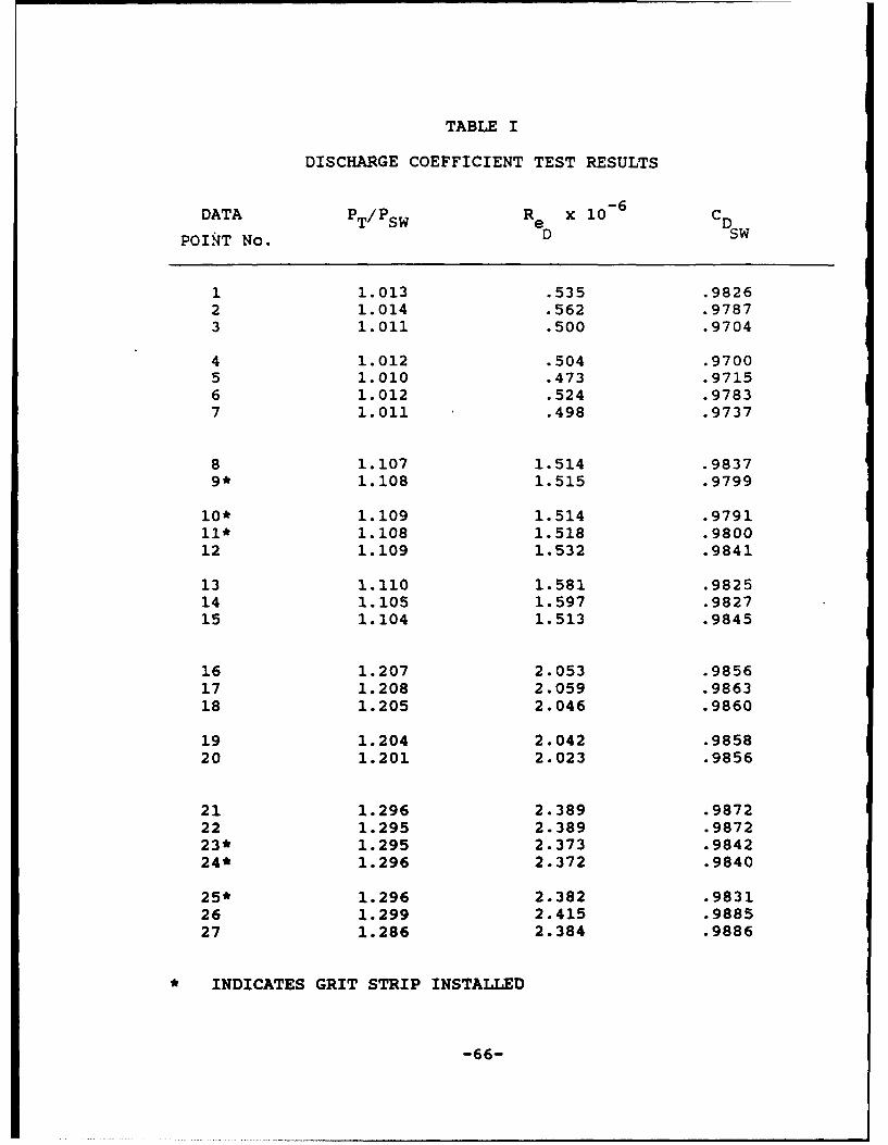
TABLE I

DISCHARGE COEFFICIENT TEST RESULTS

DATA PT/PSW Re x 10- 6 C

POINT No. D

1 1.013 .535 .98262 1.014 .562 .97873 1.011 .500 .9704

4 1.012 .504 .97005 1.010 .473 .97156 1.012 .524 .97837 1.011 .498 .9737

8 1.107 1.514 .98379* 1.108 1.515 .9799

10* 1.109 1.514 .979111* 1.108 1.518 .980012 1.109 1.532 .9841

13 1.110 1.581 .982514 1.105 1.597 .982715 1.104 1.513 .9845

16 1.207 2.053 .985617 1.208 2.059 .986318 1.205 2.046 .9860

19 1.204 2.042 .985820 1.201 2.023 .9856

21 1.296 2.389 .987222 1.295 2.389 .987223* 1.295 2.373 .984224* 1.296 2.372 .9840

25* 1.296 2.382 .983126 1.299 2.415 .988527 1.286 2.384 .9886

* INDICATES GRIT STRIP INSTALLED

-66-

TABLE I

DISCHARGE COEFFICIENT TEST RESULTS(Continued)

DATA YPTPsw ReD x 10-6 CD

POINT No.

28 1.303 2.663 .988329 1.303 2.442 .988730 1.305 2.442 .9895

31 1.351 2.562 .988932 1.353 2.565 .988833 1.352 2.560 .9888

34 1.355 2.564 .989135 1.353 2.577 .9893

36 1.399 2.689 .988837 1.403 2.698 .989538 1.401 2.693 .9892

39 1.404 2.692 .989540 1.396 2.671 .9896

41 1.501 2.908 .990242* 1.498 2.869 .987643* 1.501 2.874 .9873

44* 1.500 2.885 .987145 1.500 2.899 .990246 1.500 2.901 .9903

47 1.504 2.893 .991348 1.499 2.889 .991349 1.502 2.916 .991050 1.503 2.940 .9912

* INDICATES GRIT STRIP INSTALLED

-67-

1.004

1.000 --AA m Nominal Mach No. (M41

, 0.4to 0.5C- O0.7

0 00 0 Critical

0

0,992 030

0 -Mean Curve through0. 988I 0 Critical-Flow Data

Based on PT and Ps from 0. 125-in. -Diam Taps

0.984 '_,I I I I 1 I I0.4 0.6 0.8 1.0 2.0 4.0 6.0 8.0

Throat Reynolds Number, Re4 x 10-6

FIGURE la. ASME NOZZLE DISCHARGE COEFFICIENT BASED ON0.125-IN.DIA. THROAT TAP READINGS-COMPRESSIBLE FLOW (AIR) TESTS.

1.000 , , ,

A A A Sym Nominal Mach No. (M4)

A 0.4to 0.50o 3 0.7

2 0.995 0 0 Critical

0 00 ,0

10 0.•

9 Curve ThroughQ 0 Critical Data

Based on PT and Ps4 from 0. 125-in.-Diam Taps (Corrected)0.985 1 ( 1 13bl I f I I f 1 1

0.4 0.6 0.8 1.0 2.0 4.0 6.0 8.0

Throat Reynolds Number, Re4 x 10-6

FIGURE lb. COMPRESSIBLE FLOW ASME DISCHARGECOEFFICIENTS BASED ON CORRECTEDTHROAT TAP READINGS.

RESULTS FROM SMITH AND MATZ (REFERENCE 10) ASMESUB-CRITICAL FLOW METER CALIBRATION TEST.

-68-

0.60

0.50

0.40 -0C

~0.30

0.20

SUPERSONIC SUBSONIC

0.10

0.000.0 0.1 0.2 0.3 0.4 0.5 0.6 0.'7 0.18 O.'g 1.0 1.

Psi Po

FIGURE 2. ISENTROPIC FLOW FUNCTION, y = 1.4.

-69-

300.0

200.0

100.080.0

60.0

40.0

30.0

-. 20.0

S10.08.0

S6.0

.4.0S3.0

S2.0

0 1.0S0.8

0.6

0.4

0.3

0.2

0.1

0.050 0.2 0.4 0.6 0.8 1.0

MACH NO.

FIGURE 3. FLOW MEASUREMENT ERROR FOR 10 ERROR IN STATICPRESSURE MEASUREMENT VERSUS MACH NUMBER.

-70-

ENGINEFAN FACE

RTHROAT

1.009II1' I

o.8 . 4 I0.7

AIRFLOW 1

07I Ii It0.6 I ¼

S0.5 -

"0.4 II I~ iI0.3 tI I- II0.2 MTHAVG: .7674 1.696 .613 .507-1 .380

0.1 I I I I0.0 L J~~

0.60 0.65 0.70 0.75 0.80 0.85 0.90 0.95PS/PT

FIGURE 4. THROAT STATIC PRESSURE PROFILES.

-71-

3.0 MTRUE

0.2

0.3

2.5 ___ 0.4

0.5

2.0 0.6

~o 0.7•' 1.5

0

dc 0.8

1.0

0.9

0.5 .0.25%

00 0.01 0.02 0.03 0.04 0.05 0.06

FIGURE 5. AIRFLOW ERROR VERSUS PRESSURE COEFFICIENT.

-72-

R - STATIC PRESSURE PORTS

0.8 .8

0.4

0

U..

LaJ

0

-0.

-0.4 AT

THEORY

-1.2

X/R

FIGURE 6. HEMISPHERICAL HEAD STATIC PRESSURE PROBE

(REFERENCE 15).

-73-

o LoJ

I--

-''/-

0.36

0.32

0.28 -.

Mach AIRNumber FLOW d

0.24 0.9 4 dnl@- Xds

LaJ--

_ 0.20

S 0.16LJ•

LI0.5

0.12

0 .0 80 .

0.04

0

2 4 6 8 10 12 14

X/ds

FIGURE 8. PRESSURE COEFFICIENT VARIATION FORWARD OFPROBE SUPPORT CYLINDER (REFERENCE 17).

-75-

41, 4j 4 )J

C/R Ln

I L~r

LaLJ

C 4- ea - r

4.. s. 4 1 F.ro S- LU )

r- 4J CM 0- A aeaOU S-W f

C4f) ea

00

~nO.Juj

C-)LAJ

V)

00

LA- ILL. -

S- S- 3t

-76-.

cc -

4-4C)

La..

AjJ LLJ

00

0 . 0

C41

AA

I-s.

-77-

0

1.4

03

0)

V.)LLJ

4j1 0.

I-j

0 ON O<

C-

J/ =

-78-

C)

CI w Ao

lk = =

.r4-

Aj 0

In cc

E--

LIJ

0 Ix

iiiam I--LC) L0

r-.j

00 o-400

-79-

LiJ

cc

LA-

U-

CD0 0

-80-

1.00

0.95

0.90

0.85

0.80

0.7

0.70 120

0.60

0.55

0.500 2 4 6 8 10 1214

AXIAL STATION - INCHES

FIGURE 14. PREDICTED PRESSURE DISTRIBUTIONS.

-81-

0.020

0.015

(ild,u

he

S0.010I.-

z

o 0.005

0.0001.0 1.1 1.2 1.3 1.4 1.5 1.6

PT/PSW

FIGURE 15. PREDICTED THROAT DISPLACEMENT THICKNESS.

-82-

0.995

0990 -0-

zCLAJ0 0.985LA-

0

0.980 D WS

0.975 -

CW + .83061 + .28286(PT/Psw) - .17393(PT/PSW) 2

.70-WS + .03814(P T/PS) 3

0.970 411.0 1.1 1.2 i.3 1.4 1.5 1.6

PRESSURE RATIO - PT/PSW

FIGURE lb. DISCHARGE COEFFICIENT COMPONENTS.

-83-

1.000

0.995

NATURAL

0.990 - TRANSITIOIN

wjdo.00

0 0.985,., oo ALL TURBULENT0

0 ~~~ ~ 4 __ _ _ _ _ _ _ _ _ _

w0.980

a/

0.975 - or

0.9701.0 1.1 1.2 1.3 1.4 1.5 1.6

PRESSURE RATIO - Pr/PSW

FIGURE 17. PREDICTED DISCHARGE COEFFICIENTS.

-84-

IL

r-

aLa

i - 0

75d

-85--

I I I I Ii i-i

I-

j *" 'IS 1 I! 'I

-86-

'0 I 0I~fit

A uNJ

I Ir

AVI~27TC DTIC' DOZE N0-T F Z'IT FULLV LCOII LL. UL7CCiO

-86-

0-

-4-

:0.0

-87-

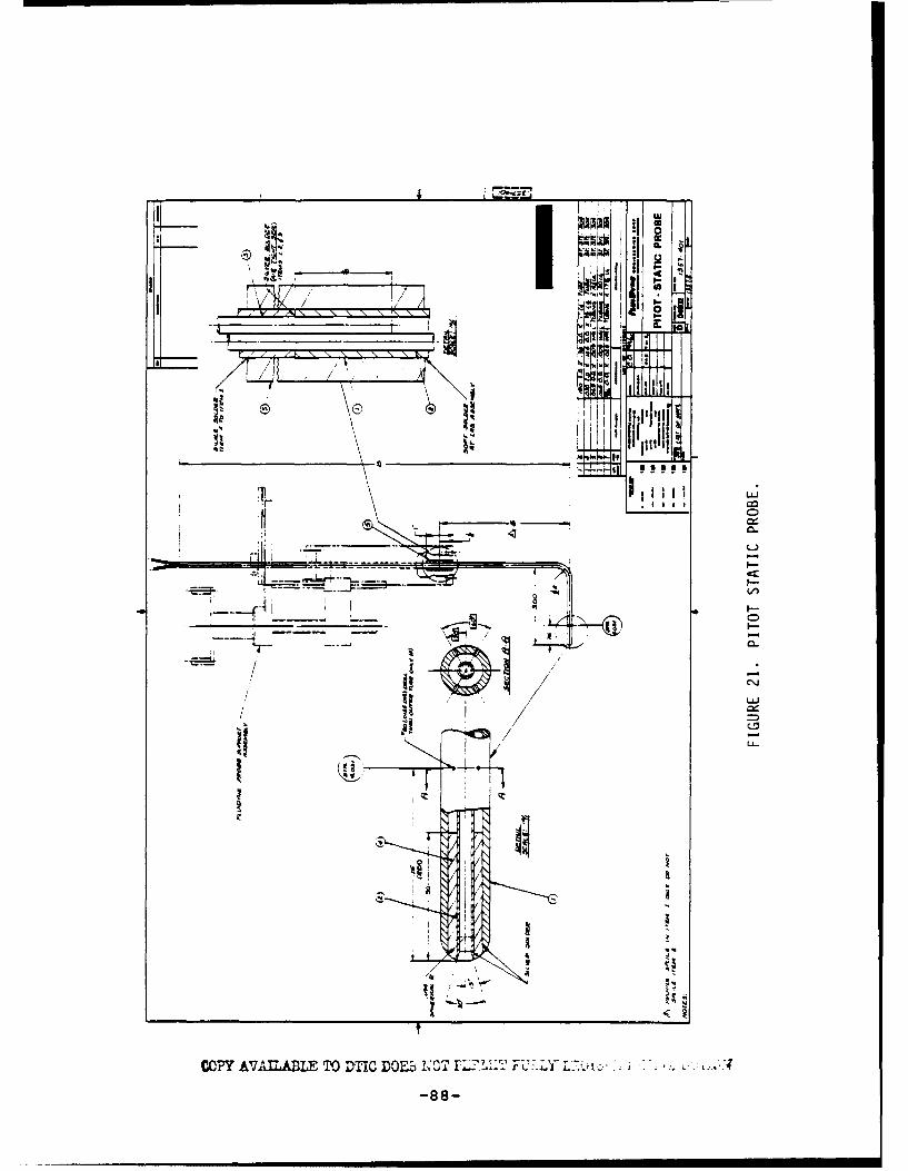
I--cc

* ~lCL

-. 4--- -. 11~i~ LILI!! / 1 ~It~

B /J

j jut~kl

-88-)

IRI

Of'

B .II.HI

*L

LU.

-89-

- -

L~ L:!IU

CAj

1" ' ýH: HHHlM +

kjCj i -;I.'I]el

9-I

I-L

C)

C)

L~CL

CL

0. r-4

6.C

C.j

La ~ ifI.1.1

z

-91-

MJET = 0.5

_TW JET

75 POIN T2•

TPOINT 1

5t

0.2 -

MJET 0.5

0.1Cp AT POINT 1FOR INFINITE

0 - WIDTH JET

z

1 -0.1

• -0.2

La.

-0.3 _Cp AT POINT 2

FOR INFINITEWIDTH JET

-0.4 -- _____ I"0 2 4 6 8 10 12 14 16

WJET/t

FIGURE 25. INFLUENCE OF CALIBRATION NOZZLE JET WIDTH ON CALIBRATIONACCURACY.

-92-

0.06

0.05

0.04

CL 0.030

0.0.02 -- -3-l

0.02 --

Cl X/ E = 0.5

L~~X/D JET = 1.0

000.0 0.1 0.2 0.3 0.4 0.5 0.65 0.7 0.8 0.9

M JET

FIGURE 26. PRESSURE SURVEY PROBE FREE JET CALIBRATION TEST RESULTS.

-93-

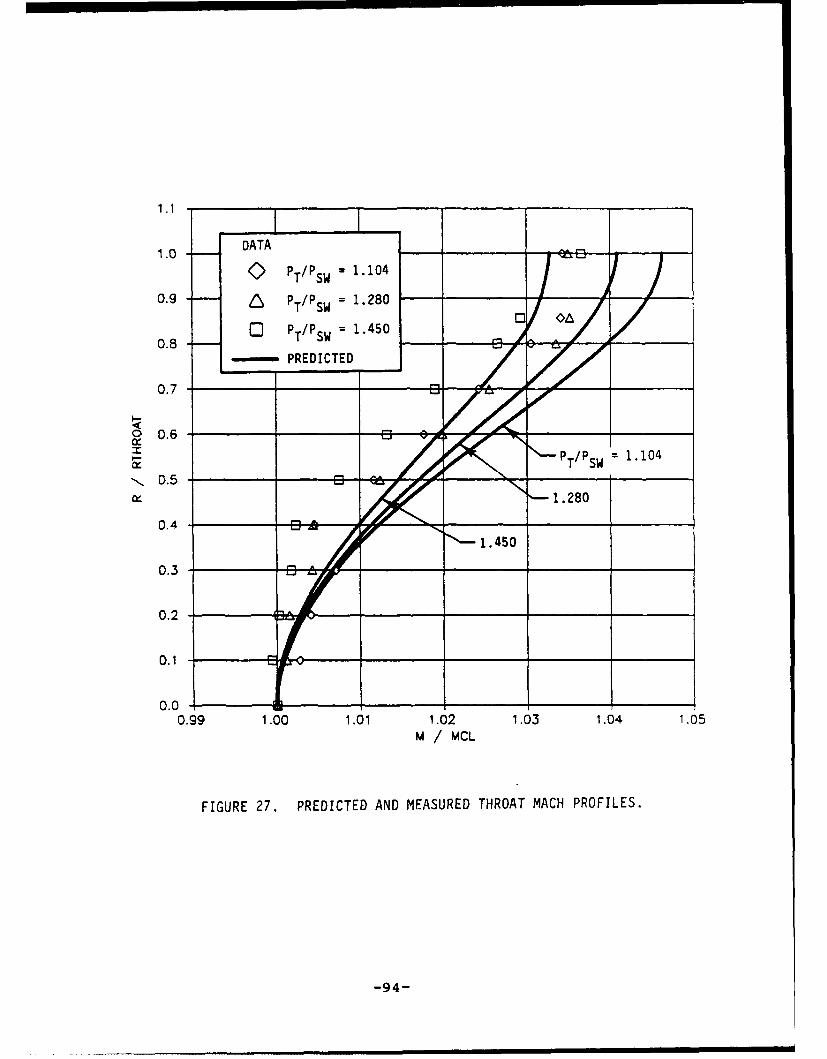
1.1

1.0 DATA _______

SPT /Psw , 1.104

0.9 ZsA ~T'S /Ps 1.280 -

0.8 0 PT/Psw = 1.450

0.7 - PREDICTED / Zo/

006-0 S0.50 0.6 4

Zoo /P 1.104

D0.5 r- "I

0.4 -I

6. 280

-4'--1.450

0.3

0.2

0.1

0.00.99 1.00 1.01 1.02 1.03 1.04 1.05

M / MCL

FIGURE 27. PREDICTED AND MEASURED THROAT MACH PROFILES.

-94-

1.000 -_ _ _ _ _ _ _ _ _ _ _ _ _ _ _ _ _ _

CDc *

0.975.D 83061 + .28286(P T/P sw) .17393(P T/P sw)2

Cws + .03814(P T/jPsw)3

0.g70

1.0 1.1 1.2 1.3 1.4 1.5 1.6PRESSUREITEAIO - MS/PSW

FIGURE 28. DISCHARGE COEFFICIENT COMPONENTS.

-95-

1.60 -

1.50

1.40

S1.30I-,

CURVEFIT

1.20

1 .2 0 '* ýT E S T D A T A

1.10

1.001.00 1.05 1.10 .15 1.20 1.25

PT/PAMB

FIGURE 29. THROAT WALL AVERAGE STATIC PRESSURE RATIO VERSUS OVERALL

PRESSURE RATIO.

-96-

1.54 • CALCULATED FROM (PT/PSW)NOMINAL - 1.45

CURVEFIT FOR NOPROBE IN PLACE

MEASURED WITHPROBE IN PLACE

1.52

S1.50U,

a-

1.48

r/R =.857

1.46 .8 .7 .6

4 .3 .24

1.441.196 1.198 1.200 1.202 1.204 1.206 1.208

PT/PAMB

FIGURE 30. SURVEY PROBE EFFECT ON THROAT WALL AVERAGE STATIC PRESSURE

RATIO.

-97-

1.32

• CALCULATED FROM (PTIPsW)NOMINAL = 1.28CURVEFIT WITH NOPROBE IN PLACE

1.31 - MEASURED WITHPROBE IN PLACE

1.30

S1.29

1.8- r/R 857 8ý .7 6• 6" 6" 6" 6 ý 54 .2 .. .. .. . ••1.28

1.27

1.261.140 1.142 1.144 1.146 1.148

PT/PAMB

FIGURE 31. SURVEY PROVE EFFECT ON THROAT WALL AVERAGE STATIC PRESSURERATIO.

-98-

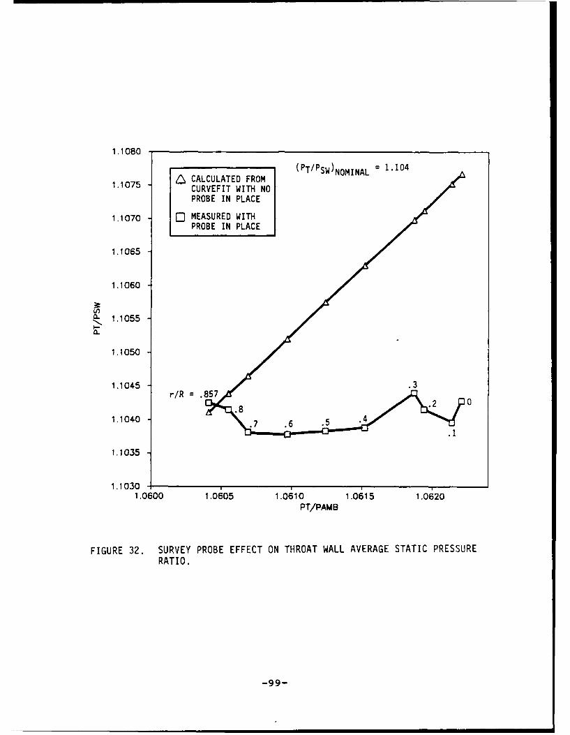
1.1080

1.1075 - CALCULATED FROM (PTIPSW)NOMINAL 1.104

CURVEFIT WITH NO

PROBE IN PLACE

1.1070 - MEASURED WITHPROBE IN PLACE

1.1065

1.1060

(I1.1055

I-.

1.1050

.8 .2 0O1.10450

1.1040-

1.1035

1.10301.0600 1.0605 1.0610 1.0615 1.0620

PT/PAMB

FIGURE 32. SURVEY PROBE EFFECT ON THROAT WALL AVERAGE STATIC PRESSURERATIO.

-99-

0.715300'

r/R -0A

0.710

0.705

0.700

-CORRECTION IMPLIED

o. 0.695 BY PROBE CALIBRATION

0.690

0.685 ±- 0.1% AIRFLOW

0.680

0.675 ...0 4.5 90 135 180 225 270 3!5 360

ANGULAR POSMTION - DEGREES

FIGURE 33. EFFECT OF SURVEY PROBE ON MEASURED THROAT STATIC PRESSURES.

-100-

0.715

r/R = 0.5 30 A0.7 10R 3•-JLJ J

R r0.705 - t

0.700 A- AAA

Q.0.695a1.

CORRECTION IMPLIEDBY PROBE CALIBRATION

0.690

0.685

0 8 ±0.1% AIRFLOW

0.680

0.675 .0 45 90 135 180 225 270 315 360

ANGULAR POSmON - DEGREES


-101-

0.715

0.710 r/R z 0.857 3 A

0.705 R r-"

0.700

a-0.6950.

0.690 0.690 •CORRECTION IMPLIED

0.685

0.680 ]

±0.1% AIRFLOW

0.67511- - 1 - - -II0 45 90 135 180 225 270 315 360

ANGULAR POSMON - DEGREES


-102-

1.000 _

0.995

0.990

o 0.9850 ogo ,,w .0

50.980 oe0

.00 PREDICTED NATURALTRANSITION

0.975 PREDICTED ALLTURBUL ENT

0 MEASURED NO BL TRIP

1 .0 1.1 1.2 1.3 1.4 1 .5 .PRESSURE RATIO - PT/PSW

4ACH NO..1 .2 .3 .4 .5 .6 .7 .8l, ,i I I I I

.4 .81 1.21 1.60 1.98 2.36 2.69 2.98REYNOLDS NO. - Reox 10-6

FIGURE 36. DISCHARGE COEFFICIENT VERSUS WALL STATIC PRESSURE RATIO.

-103-

CC.L

- I--

41 C:

00~

-L.

-104

L~owa

0.=99

10.985O_ __

PREDICTED NATURALSTRANSITION

I - I PREDICTED ALL09"5 TURBULENT

O C MEASURED NO BL TRIP

o A MEASURED WITH BL TRIP0.970 I -

1..2 1.4 151.6RESRE •RATIO - PT/PSW

MACH NO.

.1 .2 .3 .4 .5 .6 .7 .8lit I I I I.4 .81 1.21 1.60 1.98 2.36 2.69 2.98

REYNOLDS NO. - Re0 x 10-6

FIGURE 38. DISCHARGE COEFFICIENT VERSUS WALL STATIC PRESSURE RATIO.

-105-

0.14

LOG-LAW CURVE FIT

0.12 DATA, RUN 58

PT/PSW = 1.1

Cf = .00440

6* = .00752 in.

0.10 9 = .00514 in.S0.08

D-0

>. 0.06 --

0.044-

0.02 /

0.00 - ---

0.0 0.1 0.2 0.3 0.4 0.5 0.6 0.7 0.8 0.9 1.0 1.1U/UE

FIGURE 39. MEASURED BOUNDARY LAYER AT THROAT.

-106-

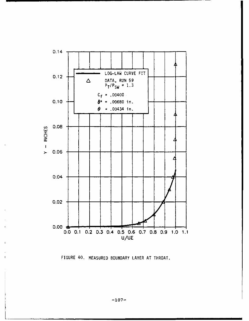
0.14 _ _ _ _ _ _ _ _ _ _ _ - - -

0.12 LOG-LAW CURVE FIT

DATA, RUN 59PT/PSW = 1.3

Cf = .00400

0.10 - P = .00680 in. -- - -

0. 08 - t9 = .0043 14 in. I

v0.08 ------------------- -

0.0

0.02 --- - - - - - - - - - -

0.00- - n n - -

0.0 0.1 0.2 0.3 0.4 0.5 0.6 0.7 0.8 0.9 1.0 1.1U/UE

FIGURE 40, MEASURED BOUNDARY LAYER AT THROAT.

-107-

0.12

LOG-LAW CURVE FIT0.10 DATA, RUN 60

PT/PSW = 1.5

Cf = .00390

6* = .00676 in.

0.08 9 = .00411 in.

'.)

z 0.06

0.04 -

0.02 /

0.000.0 0.1 0.2 0.3 0.4 0.5 0.6 0.7 0.8 0.g 1.0 1.1

u/UE

FIGURE 41. MEASURED BOUNDARY LAYER AT THROAT.

-108-

0.12

"- ' LOG-LAW CURVE FIT

0.10 DATA, RUN 66PT/PSW = 1.3

Cf = .003406* = .01052 in.

0.08 - = .00659 in.

U')

(-)'

z 0.06

0.04

0.02--

0.000.0 0.1 0.2 0.3 0.4 0.5 0.6 0.7 0.8 0.9 1.0 1.1

U/UE

FIGURE 42. MEASURED BOUNDARY LAYER AT THROAT.(EFFECT OF TRIP)

-109-

2.0

1.8

1.6 PREDICTION

PT/PSW = 1.1096

1.4 - DATA POINT 13

1.2

LuJ

S1.0

0.8

C.6

0.4

0.2

0.00.0 0.1 0.2 0.3 0.4 0.5 0.6 0.7 0.8 0.9 1.0 1.1

U/UE

FIGURE 43. PREDICTED VS MEASURED BOUNDARY LAYER PROFILE.

-110-

2.0

1.6

PREDICTION

PT/Psw = 1.30271 .4

A DATA POINT 28

1.2

S1.0

0.8

0.6

0.4

A0.2

0.00.0 0.1 0.2 0.3 0.4 0.5 0.6 0.7 0.8 0.9 1.0 1.1

U/UE


-iii-

2.0

1 .8

1.6I ,, PREDICTIONI PT/Psw = 1.5035

1.4 - DATA POINT 47

1.2

<1.0

0.8

0.6

0.4

0.2

0.00.0 0.1 0.2 0.3 0.4 0.5 0.6 0.7 0.8 0.9 1.0 1.1

u/UE


-112-

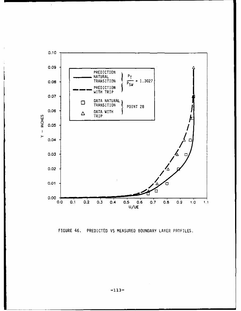
0.10

0.09 _

PREDICTIONN NATURAL ) PT

0.08 TRANSITION - 1.3027PREDICTIONWITH TRIP

0.07DATA NATURALTRANSITION POINT 28

0.06 A DATA WITHLi.) TRIP

0.05 /

0.04

0.03

0.02

0.01 A 0

0.000.0 0.1 0.2 0.3 0.4 0.5 0.6 0.7 0.8 0.9 1.0 1

U/UE

FIGURE 46. PREDICTED VS MEASURED BOUNDARY LAYER PROFILES.

-113-

PREDICTED NATURALTRANSITION

PREDICTED ALLTURBULENT

m-- PREDICTED TRIPPED0.020

E• 0 MEASURED NO BL TRIP

MEASURED WITH BL TRIP

_z 0.015

~---so-t

L,.1

0.010

0.00

1.0 1.1 1.2 1.6 1.4 1.5 1.6PT/PSW

FIGURE 47. THROAT DISPLACEMENT THICKNESS.

-114-

0.990DATA POINT 6

0.989 0 0

0.988

+ 0.1% AIRFLOW AVG.

0.987

00

3150 450

TAP LOCATIONS--1 (

2700*-.- 900

225 1350

1800

0.903 DATA POINT 13

0.902

a. 00

0.901 f [] m]

+ 0.1% AIRFLOW tAVG.

0.900 .......0 45 90 135 180 225 270 315 360

ANGULAR POSmON - DEGREES

FIGURE 48. MEASURED THROAT STATIC PRESSURES.

-115-

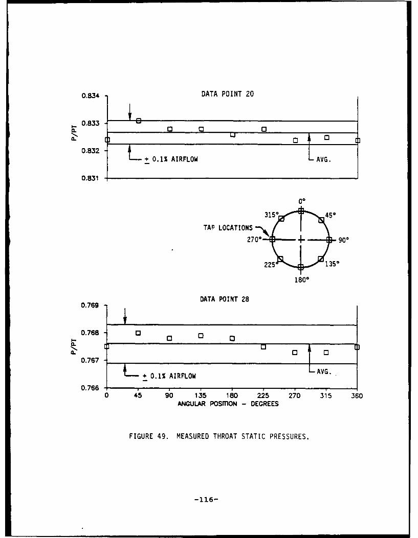
0.S34 -DATA POINT 20

0.833

3 u

0.832 - + 0.1% AIRFLOW - AVG.

0.831

00

3150 450

TAP LOCATIONS 9-0

2700 02,o 2 3o5225 • 135°

180°

DATA POINT 280.769

0.768 0

0.767

+ 0.1% AIRFLOW AVG.

0.7660 45 90 135 180 225 270 315 360

ANGULAR POSTON - DEGREES


-116-

0.715 - DATA POINT 38

0.714 - 0 f.AVG.ka.

0.713 o 0

0.712 0.1% AIRFLOW

00

3150 450

TAP LOCATIONS --

270090

225 j. 1350

180°

0.667 DATA POINT 47

S0.665 o0.666C3] AVG.

0. C01AR

0.663

0 45 9b 165 18o 25 270 315 360ANGULAR POSMON - DEGREES


-117-

1 .0 0 .ý R F R a e E 3 e s 8 : g g g g a

0.95

a- 0.90

0.85 - PREDICTION

MEASURED DATA

0 POINT 6, PT/PSW = 1.0116

<> POINT 13, PT/PSw = 1.1096

0.800 2 4 6 8 10 12 14


FIGURE 51. PREDICTED VERSUS MEASURED AXIAL WALL STATIC PRESSUREDISTRIBUTIONS.

-118-

1.00-

0.95

0.90

0.85

a- 0.80iL

0.75

0.70 PREDICTION

MEASURED DATA

0.6 Q POINT 20, PT/PSw = 1.2009

<POINT 28, PT/PSW = 1.3027

0.600 2 4 6 8 10 12 14


FIGURE 52. PREDICTED VERSUS MEASURED AXIAL WALL STATIC PRESSUREDISTRIBUTIONS.

-119-

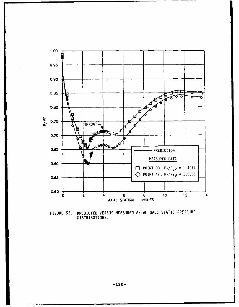
1.00-

0.95

0.90 _

0.85

0.80

S0.75

0.7

0.60M0 POINT 38, PT/PSW = 1.4014

0.55 _C) POINT 47, PT/PSw = 1.5035

0 2 4. 6 I 10 12 14


FIGURE 53. PREDICTED VERSUS MEASURED AXIAL WALL STATIC PRESSURE

DISTRIBUTIONS.

-120-

C4

m :

Wi~OZ

at-I-i V)..

0 N- C)

110 0. < 0 0 0 0m

OAVid/id

-121-

CWd

U*% -4p 4:

LUI

mg-o w0 <~ 0 c0 -,qD o z )

-04

LLU

r) e0 0) 00 (0 to Uo C0 0 0> 07 0) 0) 0) 0)0 0 0 0 al a) 0 0 )

6c 6c6 6OAVid/id

-122-

U.,L

LUJ

m l

LUJ

a. .

-123-

1. ASSUME A CRUDE GRID.

2. EVALUATE CURVATURE.

3. INTEGRATE THE CROSS-STREAMMOMENTUM EQUATION AND THECONTINUITY EQUATION TODETERMINE THE "CORRECT"STREAMLINE POSITIONS.

4. SOLVE THE MATRIX EQUATIONFOR 6n AND MOVE THE GRIDPOINTS.

FIGURE 57. SOLUTION PROCEDURE.

0-0ioll M < 1

•. •,,,1 M - 1

0- moulp M > 1

FIGURE 58. FINITE DIFFERENCE STARS FORSUBSONIC AND SUPERSONIC FLOW.

-124-

L&J

-j-

t L-J

-LJ

CD~S0w cr-

LLJr-J

10I-

W,-

-125-

APPENDIX A

The Streamtube Curvature (STC) computer program (Reference

14) was developed by General Electric for NASA Langley in

the early 1970's for calculating the inviscid transonic flow

field about nacelles and inlets. Since that time other

methods, particularly time dependent techniques, have proven

to be more successful for that purpose. However, over the

course of the past 15 years of use on a very wide variety of

aerodynamic components and configurations the program has

demonstrated a versatility for highly acc'lrate solutions for

general subsonic and supersonic planar and axisymmetric

flows. The flowfield in unchoked flow meters is a

particular example where it is felt that accuracy

improvements offered by newer methods are probably not

likely. Therefore the STC code was chosen for this program.

The STC method has not been discussed much in the open

literature, however the method is a natural one, being

similar to the way one would rely on one-dimensional

compressible flow relationships for a first order solution

to ducted flows. The STC approach however solves for a

number of confluent streamtubes, each with slightly

different properties to obtain the total flow in the

channel. In the limit, as the size of each streamtube

-126-

approaches zero, the STC method satisfies the inviscid

equations of motion exactly. The following description

extracted from Reference 14 presents key features of the

method.

The method uses a natural coordinate system. That is the

solution grid is composed of streamlines ( = constant

lines) and lines which are orthogonal to the streamlines

(4 = constant lines).

Across the streamlines, the continuity and momentum

equations are:

Continuity:

= pV

Momentum:

(a) Normal form:

a-• = ¢pv 2an

(b) Crocco form:

2 (Vn = "CV 2 + T( = Const.)an an

-127-

Along the streamlines the energy and momentum equations

are:

Momentum:

DS (x = Const.)Ds

Enercrv:

DHDH (Nf = Const.)

where, the independent variables s and n are the distances

measured along and across the streamlines, respectively.

The solution method is an extension of the streamline

curvature method. It may be briefly described as follows:

First, a crude grid of streamlines and orthogonal lines is

assumed (Figure 57); second, the curvature of the

streamlines at each of the grid points is evaluated, third,

the momentum equation is integrated along a line normal to

the streamlines to obtain velocity, and the continuity

equation is integrated to determine the "correct" streamline

positions (for the assumed curvature field). These are

indicated by the "x" in Figure 57. Fourth, an adjustment

(S n) is computed by considering: (1) the difference between

the computed and assumed streamline positions and, (2) the

effect of the implied curvature modification in the

integrated momentum equation. Finally, the streamlines are

repositioned by the an values.

-128-

Because the movement of any one grid point alters the

velocity at nearby points through a change in curvature, it

is highly desirable to account for these interrelating point

adjustments simultaneously. The utilization of a

simultaneous solution procedure, employed here, -is not part

of the classical streamline curvature method (References 20,

21, and 22). In comparison, the classical method yields

calculation times which are very slow, especially for a

closely spaced calculation grid. In concept, the set of

simultaneous equations for the normal streamline adjustments

is formulated from the finite difference equivalent of the

following equation.

a2 On) + (1-M) a2F) = F

a 2 (V)2 as2

where,

8n = Required streamline adjustment in the normal

direction

V = Stream function

s = Curvilinear distance along a given streamline

M = Mach number

PV = Flow per unit area

F = Driving (or error) function derived from the

solution to the integral continuity and normal

momentum equations

-129-

From a mathematical point of view, the above equation is

similar to the small perturbation form of the velocity

potential equation employed by Murman and Cole (Reference

23).

Y 2- - - x +

V<<1, M Ua a

In either case, it is possible to numerically solve the

equations for either subsonic flow or supersonic flow by

changing the finite difference star from a subsonic

representation to a supersonic representation as illustrated

in Figure 58. Notice that the supersonic representation

includes no points downstream of the cross-stream line,

reflecting the physical reality that disturbances downstream

will not be felt upstream. The star-switching process is

directly related to the coefficient (1- 2); and, because

this coefficient is zero at unity Mach number, the switch

from one star to the other is performed smoothly.

Considerable complexity is introduced when this equation is

expanded to allow the vertical component of velocity, v, to

be the order of magnitude of the axial component u. In this

-130-

case when the grid system is not aligned with the flow

direction, a cross-derivative term:

uv 2

a2 axa

appears in the differential equation, and the star-switching

concept (as explained above) cannot be applied. On the

other hand, with the intrinsic coordinate system utilized in

the STC procedure, the arms of the star are always oriented

in the streamwise and cross-stream directions, and the

star-switching algorithm is always appropriate.

Figure 59 shows a typical streamline/orthogonal line grid

for the flowmeter designed for this program. It is

representative of all the solutions obtained. Note that the

intersection between the downstream end of the facility

adapter pipe and the start of the contraction into the meter

has been modified slightly by the addition of a small

fillet. Although the STC program can accommodate such a

stagnation point discontinuity, experience has shown such

fillets closely duplicate the small separation bubble that

forms in this region without affecting the solution

elsewhere in the meter. This is indicated by the

comparisons of the measured and calculated pressure

distributions at X = 0 in Figures 51 - 53.

-131-

Documents

DTIC · lynn technical information center, 24001 - 3 copies lynn reports. all classes. 1 copy ... tom scott 34043 d.a. dietrich a-317 d.k. dunbar a-330