Embed Size (px)
Citation preview

Durham E-Theses
Bogomol'nyi equations on constant curvature spaces
Hickin, D. G.
How to cite:
Hickin, D. G. (2004) Bogomol'nyi equations on constant curvature spaces, Durham theses, DurhamUniversity. Available at Durham E-Theses Online: http://etheses.dur.ac.uk/3037/
Use policy
The full-text may be used and/or reproduced, and given to third parties in any format or medium, without prior permission orcharge, for personal research or study, educational, or not-for-pro�t purposes provided that:
• a full bibliographic reference is made to the original source
• a link is made to the metadata record in Durham E-Theses
• the full-text is not changed in any way
The full-text must not be sold in any format or medium without the formal permission of the copyright holders.
Please consult the full Durham E-Theses policy for further details.
Academic Support O�ce, Durham University, University O�ce, Old Elvet, Durham DH1 3HPe-mail: [email protected] Tel: +44 0191 334 6107
http://etheses.dur.ac.uk

Bogomol 'nyi Equations on Constant Curvature Spaces
D. G. Hickin
A copyright of this thesis rests with the author. No quotation from it should be published without his prior written consent and information derived from it should be acknowledged.
A the~:5is presented for the degree of
Doctor of Philosophy
Department of Niathematical Sciences University of Durham
England
July 2004
2 0 APR 2005

Dedicated to My family, for all their support over the years.

Bogomol'nyi Equations on Constant Curvature Spaces
D. G. Hickin
Submitted for the degree of Doctor of Philosophy
July 2004
Abstract
This thesis is concerned with the anti-self-dual Yang-Mills equations and their re-
ductions to Bogomol'nyi equations on constant curvature spaces.
Chapters 1 and 2 contain introductory material. Chapter 1 discusses the origin
of the equations in particle physics and their role in integrable systems. Chapter 2
describes the equations and the reduction process and outlines the construction of
solutions via the twistor transform. In Chapter 3 we consider Bogomol'nyi equations
on (2 +I)-dimensional manifolds and show that for constant curvature spa.ce-times
the equations are integrable and consider solutions in the negative scalar curvature
case. In Chapter 4 we cover the negative scalar curvature case in more detail, con
structing a number of soliton solutions including non-trivial scattering and consider
the zero-curvature limit. In Chapter 5 we consider Bogomol'nyi equations in 3-
dimensional hyperbolic space, derive an ansatz for solutions of the equation and use
it to construct a number of new solutions. Chapter 6 contains concluding remarks.

Declaration
The work in this thesis is based on research carried out at the Department of :tvlath
ematical Sciences, University of Durham, England. No part of this thesis has been
submitted elsewhere for any other degree or qualification and it all my own work
unless referenced to the contrary in the text. No originality is claimed for Chapters
1 and 2, Sections 3.1, 4.1 and 5.1, and for Appendix A.
Copyright© 2004 by D. G. Hickin.
"The copyright of this thesis rests with the author. No quotations from it should be
published without the author's prior written consent and information derived from
it should be acknowledged".
lV

Acknowledgements
I would like to thank my family for all their help and support during my PhD. I
would also like to thank my supervisor Professor R. S. Ward for his guidance, the
Engineering and Physical Sciences Council for financial support, M. Imran for his
assistance with lbT'EX, all the staff and students of the University of Durham who
assisted me during my studies, and everyone who helped me during my time at the
University of Warwick, especially lVIario Micallef.
v

Contents
Abstract
Declaration
Acknowledgements
1 Introduction
1.1
1.2
Instantons and Monopoles
Integrable Systems . . . .
Ill
lV
v
1
3
15
2 Twistors and the ASDYM Equations 18
2.1
2.2
The ASDYM Equations
Twistor Methods
. . . . . . . . . . . . 18
. . . . . . . . . . . . 21
2.3 Reductions . . . . . . . . . . . . . . . . . . . . . . . . . . . . . . . . 29
2.4 Minitwistor Spaces . . . . . . . . . . . . . . . 35
2.5 Application to Instantons and Monopoles . . . . . . . . . . . . . . . . 38
3 Bogomol'nyi Equations on Constant Curvature Space-times 50
3.1 Minkowski Space-time . . . . . . . . . . . . . . . . . . . . . . . . . . 51
3.2 Anti-deSitter Space-time . . . . . . . . . . . . . . . . . . . . . . . . . 56
3.3 deSitter Space-time ... . ................... 63
VI

304 Solutions for ADS Space-time 68
305 Bundles for ADS Space-time 0 0 0 0 0 0 0 0 0 0 0 0 0 0 0 0 0 0 0 0 0 0 0 70
4 Solutions of the Bogomol'nyi Equations on ADS Space-time 7 4
401
402
403
Solutions for Minkowski Space-time
1-Solitons 0 0 0 0
Trivial Scattering
74
80
0 0 0 0 0 0 0 0 0 0 0 0 0 0 0 85
4.4 Limiting Cases and Non-trivial Scattering 0 0 0 0 0 0 0 0 0 0 0 0 0 0 0 90
405 Zero-Curvature Limit 0 0 0 0 0 0 0 0 0 0 0 0 0 0 0 0 0 0 0 0 0 0 0 0 0 0 0 99
5 Hyperbolic Monopoles
501
502
503
504
505
506
Hyperbolic Monopoles and Instantons 0
An Ansa.tz for Hyperbolic Monopoles
1-Monopole Solutions 0
2-Monopole Solutions 0
Higher-charge Monopoles 0
Ansatze for Higher-p Monopoles
6 Outlook
Appendix
A Vector Bundles and Connections
Ao1 Vector Bundles 0 0 0 0 0 0 0 0 0
104
105
110
112
113
116
118
121
123
123
123
Ao2 Principal Bundles, Associated Bundles and the Adjoint Bundle 0 125
Ao3 Connections and Curvature 0 0 0 0 0 0 0 0 0 0 0 0 0 0 0 0 0 0 0 0 126
Bibliography 129
Vll

List of Figures
4.1 Example 4.4- II<I>II 2 for various values oft. . ..... .
4.2 Soliton paths for various values of the scale parameter a.
4.3 Example 4.4- II<I>II 2 for various values of s.
4.4 Example 4.4 - Energy density £ at t = 0. .
4.5 Example 4.5- II<I>II 2 at s = 0 for various values of a.
4.6 Example 4.6- II<I>II 2 for various values of s.
4.7 Example 4.7- II<I>II 2 at s = 0.
4.8 Example 4.8- II<I>II 2 at t = 0.
4.9 Example 4.8- II<I>II 2 at s = 0.
4.10 Example 4.9- II<I>II 2 at s = 0.64 for various values of a.
4.11 90° scattering. Example 4.10- II<I>II 2 for various values of s.
4.12 60° scattering. Example 4.11- II<I>II 2 for various values of s.
5.1 A monopole of charge 1. . . . . . .
5.2 A number of 2-monopole solutions.
5.3 An axially-symmetric monopole of charge 2.
5.4 An axially-symmetric monopole of charge 3.
5.5 A 2-monopole / 1-monopole configuration ..
Vlll
84
85
86
87
88
89
91
92
93
96
97
98
113
115
116
117
118

Chapter 1
Introduction
This thesis is concerned with the anti-self-dual Yang-Mills equations and their re
ductions, in particular their reduction to Bogomol'nyi equations.
The equations have been of interest to mathematicians and physicists for a num
ber of years. They first arose in the study of nonabelian gauge theories (Yang-Mills
theories) in elementary particle physics. These theories in their quantised form are
used to model the interaction between matter by the strong a,nd electro-weak forces.
The Euler-Lagrange equations of the theory are in general difficult to solve, however
for fields satisfying the simpler anti-self-dual Yang-Mills (ASDYM) equations the
Euler-Lagrange equations are automatically satisfied. Instantons, finite action solu
tions in Euclidean space E 4, provide the dominant contributions to the Euclidean
functional integrals and play a role in a number of calculations in the quantum
theory.
The second application of the ASDYM equations in theoretical physics is to
magnetic monopoles. These are soliton solutions of certain Yang-Mills-Riggs gauge
theories classified by a topological charge - the monopole number. In the full
quantum theory these solutions correspond to particle states. From a distance they
resemble a configuration of magnetic charges, the total charge being proportional to
the monopole number. In the limit when the Higgs potential of the theory is taken
to be zero, the Prasad-Sommerfield limit, the monopoles correspond to solutions
of the Bogomol'nyi equations in E3 and these in turn correspond to solutions of
1

the ASDYM equations in IE4 invariant under a 1-dimensional group of translations.
These are not instantons though since they have infinite action.
A key feature of the ASDYM equations is that they are an example of an in
tegrable system. Integrability is in general difficult to define, but in this case it is
a consequence of Ward's version of the twistor transform. This relates solutions of
the ASDYM equations to holomorphic vector bundles over a complex 3-manifold,
the twistor space, which is all or part of the complex projective space CJPl3 . The
Bogomol'nyi equations in IE3 are integrable since they are obtained from the AS
DYM equations by imposing symmetry. This reduction takes place at the twistor
level too -the solutions correspond to holomorphic vector bundles over a complex
2-manifold, namely the holomorphic tangent bundle of the Riemann sphere.
This suggests a programme of obtaining integrable systems from the ASDYM
equations by imposing (conformal) symmetries. A number of well known integrable
systems, including the Korteweg-deVries (KclV), nonlinear Schrodinger (NLS) and
sine-Gordon (SG) equations, can all be obtained this way. By considering ASDYM
fields in (2 + 2)-dimensions invariant under a 1-dimensional group of translations, we
can obtain solutions ofthe Bogomol'nyi equations in (2 + 1 )-dimensional space-time.
Again these solutions correspond to bundles over the holomorphic tangent bundle
of the Riemann sphere (but the conditions which are needed to ensure real solutions
are different).
The Bogomol'nyi equations make sense in curved space-times but in general are
not integrable. However we shall show in this thesis that when the space-time has
constant curvature the equations are indeed integrable. There are three standard
space-times of constant curvature classified by whether the scalar curvature is zero,
positive or negative. These are rviinkowski space-time, which was mentioned ear
lier, deSitter space-time and anti-deSitter space-time respectively. The Bogomol'nyi
equations can be obtained from the ASDYM equations by imposing symmetry un
der "rotations" in the case of deSitter space-time and "Lorentz boosts" in the case
of anti-deSitter space-time. The solutions correspond to bundles over the reduced
twistor space, which is CJPl1 x CJPl1. This is analogous to the situation on Riemannian
2

3-manifolds. The Bogomol'nyi equations on hyperbolic 3-space, a space of constant
curvature and negative scalar curvature, can be obtained by imposing rotational
symmetry on ASDYM fields in Euclidean space.
vVe shall now review two of the main motivations for studying ASDYM equations,
namely Yang-Mills theories and integrable systems.
1.1 Instantons and Monopoles
Before discussing the two classes of solutions of nonabelian gauge theory in which we
are interested, namely Yang-Mills instantons and BPS monopoles, we shall outline
the basics of gauge theories. There are a number of good references for gauge theories
such as [1, 2, 3, 4]. We shall focus on classical gauge theories, the quantum theory
is described in many references such as [5]. The role of solitons and instantons is
described in [6]. There are a number of good reviews of monopoles including [7] and
[8].
Gauge Theories
Gauge theories are generalisations of Maxwell's theory of electromagnetism. The
essential feature is that these theories are invariant locally under a Lie group of in
ternal symmetries. In the case of Maxwell theory the Lie group is U(1). Nonabelian
gauge theories or Yang-Mills theories involve replacing U ( 1) with a nonabelian Lie
group. Such theories are used to model not just electromagnetic forces but also the
strong and weak nuclear forces. The theory is attractive mathematically - gauge
theory is most naturally described by the language of differential geometry.
Let :MrHI be (3 + 1 )-dimensional Minkowski space-time. This is JR4 with coordi-
2 2 2 2 2 ds = ch0 - d:c1 - dx2 - cha .
Let G be a Lie group with Lie algebra g. A gauge potential A= AJ.Ld:z)1 is a 1-form
taking values in the Lie algebra. The field strength corresponding to A is a g-valued
3

To define a Lagrangian one needs a Killing form, that is to say an inner product
( ·, ·) on g. One then defines the Lagrangian of pure Yang-Mills theory to be
If G is SU(N) then its Lie algebra consists of traceless skew-symmetric N x N
matrices and the Killing form is
1 (A, B)= - 2tr(AB).
The Lagrangian is then
The action S is the integral of the Lagrangian and can be written in terms of forms
as
S = ~ J tr(F 1\ *F),
where * is the Hodge star
If g is a G-valued function on Jvf, one can consider the transformation
(1.1)
under which the field strength transforms as
F',w -----+ 9 -l F',1v 9 ·
In particular, if F',w = 0 then AJL = g- 1 o~'g for some g. Transformations of this kind
are called gauge transformations and preserve the Lagrangian.
So far we have only considered pure gauge theory. To couple fields to the gauge
field one uses the principle of minimal coupling. One considers a collection of fields,
which must be representations of the gauge group, and replaces ordinary derivatives

811 in the Lagrangian with covariant derivatives Dw For example, if a field <I> is in
the fundamental representation, i.e. is column vector-valued, then
and if <I> is in the adjoint representation, i.e. taking values in the Lie algebra of G,
then
Under gauge transformations ( 1.1), <I> and its covariant derivative transform as
for the fundamental representation and
for the adjoint representation. The commutator [D11 , Dv]<I> is F{tv<I> for the funda
mental representation, and [ F,w, <I>] for the adjoint representation.
One example is QCD where one has an SU(3) gauge field and Dirac spinor fields
in the fundamental representation coupled to it. Another example which will be
important to us is a Yang-Mills-Higgs theory. One can consider a gauge field and a
scalar field, a Higgs field, in the adjoint representation, with Lagrangian
1 1 .C = --(F F/1v) + -(D <I>.D11 <I>)- V(<I>) 4 /1V1 2 /1 '
for some function V.
A key feature of gauge theories is the possibility of spontaneous symmetry break
ing. This occurs when the ground state or vacuum of the theory is degenerate. A
given choice of ground state is not preserved by the full gauge group but by a sub
group H called the residual group. We say the gauge group G is broken to H.
One then considers perturbations around this ground state. For example in the
Weinberg-Salam model of electro-weak theory SU(2) x U(1) is broken to U(1). This
5
mechanism gives masses to some of the gauge particles, which would otherwise be
massless since mass terms are not gauge invariant. In the Yang-Mills-Higgs the
ory above with gauge group SU(N) if the set of minima of V is degenerate and a
ground state has eigenvalues A1, ... , A,. with degeneracies N1 , ... , N,. then SU(N) is
broken to SU(Nl) x ... x SU(N,.) x U(ly- 1• This is of interest in Grand Unified
Theories (GUTs), which are an attempt to unify the strong and electro-weak forces.
An example is SU(5) gauge theory, which, when N 1 = 3, N2 = 2, is broken to
SU(3) X SU(2) X U(l).
Let us consider classical solutions of these theories, I.e. solutions of the Euler
Lagrange equations for critical points of the Lagrangian (of course one must consider
the quantum theory to get any realistic understanding of the theory, but we shall
not do this here). For pure Yang-Mills theory the Euler-Lagrange equations are
in other words,
D ptw = 0 !l '
where of course D*F _ d*F + [A, *F], D 11F
automatically satisfies the Bianchi identity
DF=O,
or in components,
o11 F + [A 11 , F]. The gauge field
Thus if *F = AF for a constant A, then the Bianchi identity implies D*F = 0, and
thus the Euler-Lagrange equations of the theory are satisfied. However for a two
form B on .lVIinkowski space-time, **B = - B, and A would have to be ±'i. So for
real gauge groups, which include groups such as SU(N) in which we are particularly
interested, there are no solutions except for the trivial case when F = 0. One way
around this is to consider gauge fields on Euclidean space. We shall consider this
possibility later.
For the Yang-Mills-Higgs theory above the Lagrangian gives Euler-Lagrange
6

equations
!1 av D 11 D <I>+ o<I>
DI,<I>
The objects discussed in the previous section - gauge potentials, field strength
and so on - can be most naturally described in the language of differential geome
try. The operator D11 defines a connection on a bundle E over IV! with curvature F.
Fields coupled to the gauge field are sections of associated bundles over A1. Gauge
transformations correspond to bundle automorphisms, or locally to changes in the
choice of trivialisations of the bundle. Alternatively, one can describe the theory in
terms of principal bundles. The gauge potential A is the pullback of a connection
1-form on a principal bundle P over A1 under a section s of the bundle, F is the
pullback of the curvature 2-form on P, a. gauge transformation is a bundle automor
phism or locally is equivalent to a. choice of section s. Again the fields coupled to
the gauge field are sections of associated bundles. When Minkowski space-time is
replaced by a (general) 4-manifold these geometric and topological considerations
become important.
Yang-Mills Instantons
As was mentioned previously, for real gauge groups there are no non-trivial solutions
of *F = >..F for Minkowski space-time. However for a 2-form Bon Euclidean space
IE4, **B = B. Thus if we define gauge theories on IE4 , then ).. = ±1, and there
is the possibility of non-trivial solutions. When *F = F the Yang-Mills field is
said to be self-dual, and when *F = - F, anti-self-dual, and these equations are
the self-dual and anti-self-dual Yang-Mills equations respectively. The extension of
gauge theories from Minkowski space-time to Euclidean space is straightforward.
One simply replaces the l'vlinkowski metric with that of Euclidean space, using it in
particular to raise and lower indices. It is also customary to define the Euclidean
action density to be
7

so that it is positive definite. The Euclidean action is then
S = -IIFII 2 =- tr(F 1\ *F). 1 1 J 4 8
It is not entirely obvious what role such solutions should play in gauge theory, since
they are, after all, solutions on Euclidean space IE4. The reason is that in the QFT
of Yang-Mills fields one is interested in functional integrals of the form
J D[A JeiS'[A!'J P(A ). J.l p '
where S is the action of the theory, P a polynomial m A 11 , D[A 11 ] is a suitable
measure and the integral is taken over a suitable space of fields. These integrals are
not well-defined, however we can analytically continue to IE4 , the integrals becoming
An example is in determining the true vacuum of Yang-Mills theory. The classical
vacua of the theory occur when FJ.lV = 0, i.e. when A is a pure gauge g- 1811 g.
In quantising the theory we choose a gauge with A0 = 0 and assume g -----7 1 at
infinity. Thus g extends to a map from 5 3 to the gauge group which we shall assume
is SU(2). Such maps are classified up to homotopy by 1r3 (S3 ) rv Z. The integer N
labelling the class is given by
Around each homotopy sector one constructs a vacuum state IN). These states are
not orthogonal and tunnelling takes place between states. This tunnelling amplitude
between the N- and N+ states is determined by the Euclidean function integral
where the integral is taken over Euclidean gauge fields which tend to pure gauges in
the N± sectors as x0 tends to ±oo. The dominant contributions of such integrals will
be provided by the critical points of the action, and in particular the local minima.
These critical points are of course given by the Euler-Lagrange equations.
8

Uhlenbeck [9] showed that if we have a gauge potential on IE4 with finite action,
then it extends to the 1-point compactification of IE4 , namely the 4-sphere S4 . In
other words, there is bundle E over S4 and connection D which extends the connec
tion on IE4. Thus we are interested in connections on S4 which satisfy the Yang-Mills
equations. Such solutions are called instantons. For simple gauge groups G, such
as SU ( N), the bundles over S4 are classified by a topological invariant, the second
Chern class c2 (E), given by
The integer k = -c2 (E) is called the instanton number.
Recall that self-dual and anti-self-dual gauge-fields are critical points of the ac
tion. In fact they are local minima. If we split F into its self-dual and anti-self-dual
parts, i.e. F = F+ + F- where F± = ~(F ±*F), then substituting into the expres
sion for instanton number and action we have
and thus the action is bounded below by 8n2 lkl with equality when F is self-dual, for
k 2: 0, and anti-self-dual, for k :::; 0. One can define the instanton number in terms of
the gauge potential at infinity. The condition of finite action F11 v = 0 on the 3-sphere
S:3 at infinity, so it is a pure gauge, i.e. A11 = g- 1811g. Maps from S3 to SU(N) are
classified up to homotopy by n3 ( S U ( N)). In more geometric language, to define a
connection on S4 one covers the 4-sphere with two 'hemispherical' coordinate patches
whose intersection is a thickening of the equator S 3 and defines gauge potentials on
each patch. On the intersection the potentials differ by a gauge transformation
whose homotopy class is aga,in classified by 7r:3 ( SU ( N)).
Now one can write (see [3, 4])
tr(F 1\ F) 2
d(tr(A 1\ clA + -A3))
3 1
d(tr(A 1\ F- -A3)).
3
9
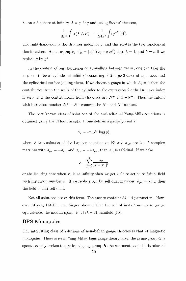
So on a 3-sphere at infinity A= g- 1dg and, using Stokes' theorem,
8~2 J tr(F 1\ F) = -241112 J (g-ldg f
The right-hand-side is the Brouwer index for g, and this relates the two topological
classifications. As an example, if g = i:ri-L(x0 + Xjaj) then k = 1, and k = n if we
replace g by gn.
In the context of our discussion on tunnelling between vacua, one can take the
3-sphere to be a 'cylinder at infinity' consisting of 2 large 3-discs at :r0 = ±oo and
the cylindrical surface joining them. If we choose a gauge in which A0 = 0 then the
contribution from the walls of the cylinder to the expression for the Brouwer index
is zero, and the contributions from the discs are N+ and - N-. Thus inst.antons
with instanton number N+ - N- connect the N- and N+ sectors.
The best known class of solutions of the anti-self-dual Yang-Mills equations is
obtained using the t 'Hooft ansatz. If one defines a gauge potential
where ¢ is a solution of the Laplace equation on IE4 and a1w are 2 x 2 complex
matrices with a 11 ,/ = -a v 11 and a 11v = -*a 11 v, then A~, is self-dual. If we take
k A. c/J= L a 2
IX- Xal
a=O
or the limiting case when x 0 is at infinity then we get a finite action self-dual field
with instanton number k. If we replace a~w by self-dual matrices, a 11v = *a 11v then
the field is anti-self-dual.
Not all solutions are of this form. The ansatz contains 5k- 4 parameters. How
ever Atiyah, Hitchin and Singer showed that the set of instantons up to gauge
equivalence, the moduli space, is a (8k- 3)-manifold [10].
BPS Monopoles
One interesting class of solutions of nonabelian gauge theories is that of magnetic
monopoles. These arise in Yang-Mills-Riggs gauge theory when the gauge group G is
spontaneously broken to a residual gauge group H. As was mentioned this is relevant
10

in, for example, Grand Unified Theories. The solutions are classified topologically
by 1r2 (G/ H). The simplest case is G = SU(2), and we shall concentrate on this.
Consider an SU(2)-gauge field with an adjoint Higgs,
This has a minimum energy solution A{, = 0, <I> = <I>0 for a constant <I>0 with II <I> II = 1.
Under a gauge transformation, <I>0 -. g- 1<I>0g so is preserved by a U(l) subgroup
of SU(2), namely by those g of the form exp (x<I>) for a real number X· In other
words, SU(2) is broken to U(l). The residual symmetry group is identified with the
gauge group of electromagnetism, and one can define electric and magnetic fields by
where <I> is <I>/II<I>II, Ei = Poi and Bi = *Poi = ~EijkpiJ. We shall be interested in
solutions which are static and purely magnetic, in other words, A0 = 0, and <I> and
Ai are independent of the time coordinate :r0 . The energy density is thus
Finite energy implies II<I>II -> 1 as lxl -> oo, and so are we have a. map from the
2-sphere at infinity to the unit 2-sphere in the Lie algebra. of SU(2). Topological
solutions are classified up to homotopy by 1r2 (S2) ~ Z, in other words by an integer
n which is the winding number or Brouwer degree of the map, which is given (see
[11]) by
This n, in the context of monopoles, is called the topological charge or monopole
number. Note since SU(2) acts transitively on the unit sphere S 2 in su(2) with
stabiliser U(l), the sphere can be identified with the coset space SU(2)/U(l), and,
by a standard result of algebraic topology (see [5]),
11

On the sphere at infinity bi = ~tr(Bi<P). So one can compute the magnetic charge
Thus the topological charge is proportional to the magnetic charge.
An argument due to Bogomol'nyi [12] allows us to estimate the energy of the
configuration in terms of the topological charge. If we expand the inequality
and substitute into the energy, then we obtain
The energy satisfies
E 2: j 1A(1- II<PII 2)
2d3x ± 81rn,
with equality if and only if Bi = =t=Di<P.
Now let us consider solutions of the theory. T'Hooft and Polyakov constructed
a spherically symmetric monopole of charge 1 in terms of radia.l profile functions
by applying an existence theorem for ODEs. The solution cannot be expressed in
terms of elementary functions for A > 0. However Prasad and Sommerfield showed
[13] that when A = 0 the gauge potential and Higgs field are given by
. sinh r- r -'lEijkOjXJ.: 2 . h ,
T Sill T
r cosh r - sinh r UljXj
T 2 sinh T
where T is the radial distance in IE3 . From now on we shall concentrate on the
limiting case with A = 0, but retaining the boundary condition II<PII = 1 at. infinity,
the Prasad-Sommerfield limit. In this case the energy estimate is saturated and so
12

such solutions are stable. The fields satisfy the Bogomol'nyi equations and such
solutions are called Bogomol'nyi-Prasad-Sommerfield (BPS) monopoles.
The energy density can be calculated from the Higgs field alone, since the Bianchi
identity DiBi = 0 and the Bogomol'nyi equations imply
where 6. = aiai is the Laplacian in IE:3 , so that
The energy density of the t'Hooft-Polyakov monopole is localised around, and
takes its maximum value at, the origin, and the Higgs field <.P has a zero there.
A general n-monopole solution has n zeros counted with multiplicities (see [11]),
and one regards a zero of ci> as the location of a monopole. The set of gauge
equivalence classes of smooth, charge n. solutions is a ( 4n -1 )-manifold Iv!n [14]. For
the 1-rnonopole these 3 parameters are the position coordinates of the centre. The
dimension of J\111 is more obvious for n ~ 2 if one considers the gauge transformations
with g = exp (x<P) for real X· If one takes x to vary linearly with time, then one
obtains a dyon, a configuration with both electric and magnetic charges, and x can
be thought of as a conjugate variable to electric charge. One should think of BPS
n-monopoles as configurations of n 1-monopoles, at least when the monopoles are
widely separated. Each monopole is determined by 3 position coordinates and a
phase. After removing a global phase we are left with 4n- 1 parameters.
For G = SU(N) one assumes <.P is asymptotically in the gauge orbit of
with p. 1 ~ {t2 ~ · · · ~ !LN and JLI + {t2 + · · · PN
symmetry breaking), H = U(1)N-I and
0. For distinct fti (maximal
1r2(SU(N)jU(l)N-!) ~ 1r2(U(l)N-l) ~ zN-I
13

Asymptotically the Higgs field is
and the topological charges are n 1 , n 1 + n 2 , ... ,n1 + · · · nN-1·
14

1.2 Integrable Systems
The ASDYM equations, as we mentioned earlier, are an example of an integrable
system, by virtue of the twistor construction which we shall outline in Chapter 2.
The equations in fact play an important role in the study of integrable systems since
a great many equations can be obtained from the ASDYJVI equations by imposing
symmetry and inherit the integrability of the original system as a result. As Ward
puts it [15]
"many of the ordinary and partial differentwl equations that are regarded as being
integrable 01' soluble may be obtained .fmm the (anti-Jsel.f-dual gauge field equations
(or its generalisations) by reduction. "
In general integrability is difficult to define, hence the phrase "regarded as being
integrable". The subject consists largely of examples and techniques which apply to
them- techniques which do not always readily extend from one system to another.
For Hamiltonian systems of classical mechanics the notion of integrability is rel
atively straightforward. A 2n-dimensional system is completely integrable if one can
find functions F1 ••• Fn which Poisson commute with the Hamiltonian of the system
and each other and whose differentials are linearly independent. The level surfaces
of these functions when compact are n-tori. If Q1 ... Qn are angular coordinates on
the tori then one can replace F1 ... Fn with functions P 1 ... Pn, which again Poisson
commute with the Hamiltonian and each other and have linearly independent dif
ferentials, such that { Qi, P1} = biJ. VVith respect to these action-angle coordinates
the equations of motion are
c!P dt
1
= O, c!Qi 8H --=-=constant. cit 8Pi
The situation is more complicated in infinite dimensions. One can take a similar
phase-space approach, which requires the imposition of bouncla,ry conditions. This
is not so satisfactory since integrability should be a property of the equation and not
depend on the boundary conditions. This approach also cannot be easily extended
to elliptic equations or equations of other signatures. A number of properties are
often possessed by integrable systems though. One has methods of constructing
15
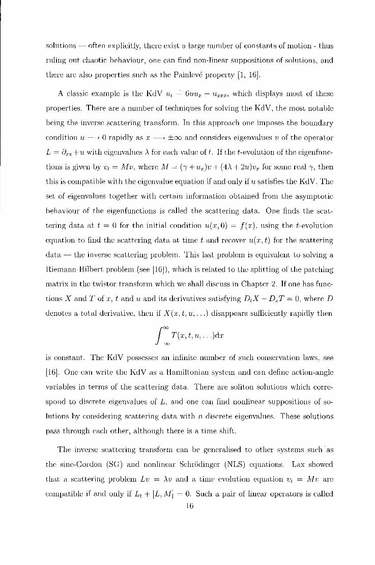
solutions - often explicitly, there exist a large number of constants of motion - thus
ruling out chaotic behaviour, one can find non-linear suppositions of solutions, and
there are also properties such as the Painleve property [1, 16].
A classic example is the KdV 'Llt ~ 6'U'Ux + 'Uxxx, which displays most of these
properties. There are a number of techniques for solving the KdV, the most notable
being the inverse scattering transform. In this approach one imposes the boundary
condition ·u ~ 0 rapidly as :c ~ ±oo and considers eigenvalues v of the operator
L = Bxx +v with eigenvalues ,\ for each value oft. If the t-evolution of the eigenfunc
tions is given by v1 = !vi v, where Pvf = ( 1 + 'Llx )v + ( 4,\ + 2'U )vx for some real1, then
this is compatible with the eigenvalue equation if and only if ·u satisfies the KdV. The
set of eigenvalues together with certain information obtained from the asymptotic
behaviour of the eigenfunctions is called the scattering data. One finds the scat
tering data at t = 0 for the initial condition ·u(x, 0) = J(x), using the t-evolution
equation to find the scattering data at time t and recover 'U(x, t) for the scattering
data - the inverse scattering problem. This last problem is equivalent to solving a
Riemann-Hilbert problem (see [16]), which is related to the splitting of the patching
matrix in the twistor transform which we shall discuss in Chapter 2. If one has func
tions X and T of .T, t and ·u and its derivatives satisfying DtX + DxT = 0, where D
denotes a total derivative, then if X ( :r, t, ·u, ... ) disappears sufficiently rapidly then
1: T(:c, t, ·u, .. . )d:r
is constant. The KdV possesses an infinite number of such conservation laws, see
[16]. One can write the KdV as a Hamiltonian system and can define action-angle
variables in terms of the scattering data. There are soliton solutions which corre
spond to discrete eigenvalues of L, and one can find nonlinear suppositions of so
lutions by considering scattering data with n discrete eigenvalues. These solutions
pass through each other, although there is a time shift.
The inverse scattering transform can be generalised to other systems such· as
the sine-Gordon (SG) and nonlinear Schrodinger (NLS) equations. Lax showed
that a scattering problem Lv = ,\v and a time evolution equation Vt = J\1 v are
compatible if and only if L 1. + [L, JV!] = 0. Such a pair of linear operators is called
16

a Lax pair. Most integrable systems are solved by writing them as compatibility
conditions for a system of linear equations, although they may be more general
systems than those considered by Lax. The KdV can be obtained from the ASDYM
by reduction (although the Lax pair above is different from that obtained from the
ASDYM equations) as can the SG, NLS, the Minkowski space-time Bogomol'nyi
equations and the integrable chiral equation. These last two related systems have a
Lax pair which we shall describe in Section 3.1. One approach to this system uses
the 'Riemann method with zeros' to generate solutions of the linear system rather
than the inverse scattering transform. These systems have soliton solutions which
can be superposed to obtain multi-soliton solutions which pass through each other
and solutions which exhibit goa scattering. There is a conserved 'energy' density in
the case of the integrable chiral model as well as an infinite number of conservation
laws.
17

Chapter 2
Twistors and the ASDYM
Equations
In this chapter we shall describe the solutions of the ASDYrvi equations, and their
reductions, by the twistor transform. Twistors were first introduced by Roger Pen
rose in his paper "Twistor Algebra" [17]. The aim of the twistor programme was
to describe the equations of mathematical physics using objects called twistors. In
this approach the twistors are the fundamental objects of the theory and the space
time points, which are usually regarded as fundamental, are derived from them.
There is an extensive literature from this viewpoint (see for example [18]). From the
viewpoint of this thesis we shall concentrate on the role of twistors in the ASDYl'vi
equations and integrable systems. The references closest to this point of view are
[1] and [2]. The ASDYM equations are best described in terms of connections on
vector or principal bundles and these are described in the appendix.
2.1 The ASDYM Equations
Let D be connection on a vector bundle E over a smooth manifold J\1 with metric
g of Riemannian, Lorentzian or ultrahyperbolic ( + + --) signature. D is self-dual
18
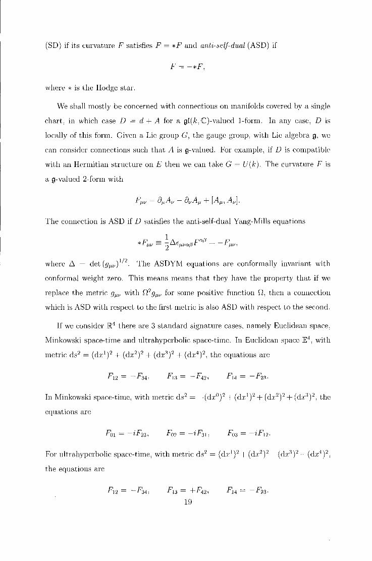
(SD) if its curvature F satisfies F = *F and anti-self-dual (ASD) if
where * is the Hodge star.
We shall mostly be concerned with connections on manifolds covered by a single
chart, in which case D = d +A for a gt(k, C)-va.lued 1-form. In any case, D is
locally of this form. Given a Lie group G, the gauge group, with Lie algebra g, we
can consider connections such that A is g-valued. For example, if D is compatible
with an Hermitian structure onE then we can take G = U(k). The curvature F is
a g-valued 2-form with
The connection is ASD if D satisfies the anti-self-dual Yang-Mills equations
where ~ = det (g1w) 112. The ASDYM equations are conformally invariant with
conformal weight zero. This means means that they have the property that if we
replace the metric g11 v with D2 g11 v for some positive function D, then a connection
which is ASD with respect to the first metric is also ASD with respect to the second.
If we consider ~4 there are 3 standard signature cases, namely Euclidean space,
}.;Iinkowski space-time and ultrahyperbolic space-time. In Euclidean space IE4, with
metric ds2 = (d1:1)
2 + (dx2)
2 + (dx3)
2 + (dx4)
2, the equations are
equations are
the equations are
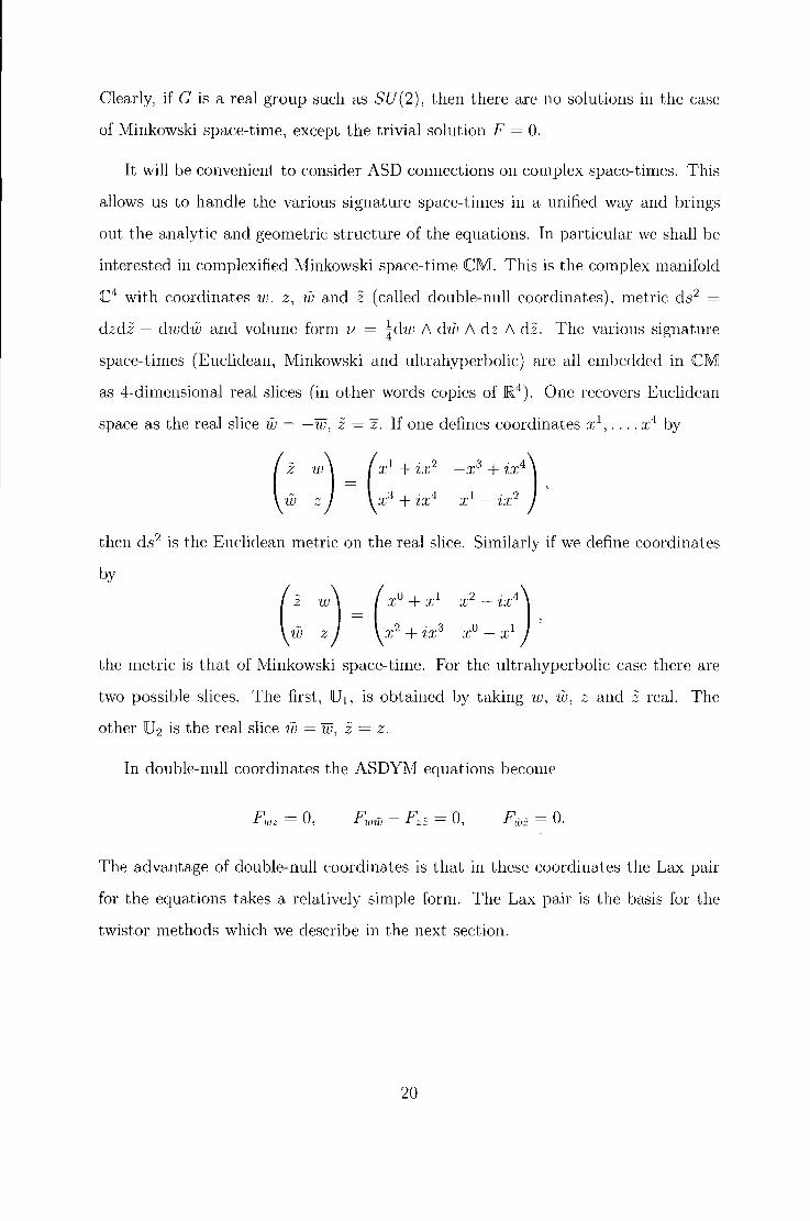
Clearly, if G is a real group such as SU(2), then there are no solutions in the case
of Minkowski space-time, except the trivial solution P = 0.
It will be convenient to consider ASD connections on complex space-times. This
allows us to handle the various signature space-times in a unified way and brings
out the analytic and geometric structure of the equations. In particular we shall be
interested in complexified Minkowski space-time <CM. This is the complex manifold
C4 with coordinates w, z, 1LJ and z (called double-null coordinates), metric ds2 =
dzdz - dwdw and volume form v = ~dw 1\ chiJ 1\ dz 1\ dz. The various signature
space-times (Euclidean, Minkowski and ultrahyperbolic) are all embedded in CM
as 4-dimensional real slices (in other words copies of JR4 ). One recovers Euclidean
space as the real slice ·w = -w, z = z. If one defines coordinates ;r1 , ... , :r4 by
3 . 4) -x +zx '
x· 1 - ix2
then ds2 is the Euclidean metric on the real slice. Similarly if we define coordinates
by
(z w) = (xo + :1:
1 x2- ix4) ' w z x 2 + ix3 :r0 - x 1
the metric is that of Minkowski space-time. For the ultrahyperbolic case there are
two possible slices. The first, 1U 1, is obtained by taking w, u), z and z real. The
other 1U2 is the real slice iu = w, i = z.
In double-null coordinates the ASDYM equations become
Pwz = 0, Pw:z = 0.
The advantage of double-null coordinates is that in these coordinates the Lax pair
for the equations takes a relatively simple form. The Lax pair is the basis for the
twistor methods which we describe in the next section.
20

2.2 Twistor Methods
Lax Pairs
The ASDYM equations are equivalent to [L, Af] = 0, where
L = Dw- C,D:z, !VI = Dz - ( D(;,.
This is the compatibility condition for the over-determined linear system
L.s = 0, !VIs= 0
to have a solution for each value of(. If l andrn are respectively the vectors Ow -(82 ,
82 - (ou, in CM then the compatibility condition is equivalent to F(l, rn) = 0. If one
replaces l and m, by linear combinations l', rn' of l and m then F (l', m') is still zero
(but L' = D,, and Jd' = Dm' only commute modulo linear combinations of L' and
!VI'). Thus the equations are a statement about a certain family of planes, namely
that the restriction of the curvature to the planes spanned by the vectors l and m
1s zero.
Let us consider these planes in more detail. A 2-plane in CM is totally null
if for all vectors X, Y in the plane g(X, Y) = 0. Given vectors spanning a plane
1T = X 1\ Y is determined up to a scalar multiple by the plane. If the plane is
null then *1T"v = ±1r 11v. (This is because 1T is determined up to scalar multiple by
the condition 1T11vX 11 = 0 for all vectors X in the plane. However for null planes
1Ti'vX~' = 0 and thus 1f1w = A1Ti'v· Since**= 1, ).. = ±1.) This divides null 2-planes
into 2 families of planes - self-dual or a-planes for which 1T1w = *1T fLV and anti-self
dual or beta-planes for which 11 11 v = -*11 11v. Connections are ASD if the curvature
vanishes on a-planes (and SD if it vanishes on ,6-planes).
Self-dua1 planes through a given point form a !-parameter family, parameterised
by (. In fact the set of a-planes through a given point is a Riemann sphere. The
quantities
).. = (w+i, p.=(z+w
are annihilated by l and m and so are constant on an a-plane with parameter (.
Since an a-plane Z is of codimension-2, ).. and ~l together with ( determine Z and
21

the set of a-planes is a (complex) 3-manifold P with local coordinates A, Jl and(.
The set of pairs of points x in CM and a-planes Z through them is a 5-manifold
:F with coordinates w, w, z, z and (. There is an obvious projection map from :F
to CM taking a typical point ( x, Z) in :F to the point x and in local coordinates
(w, w, z, z, () which is obtained by ignoring the ( coordinate. The compatibility
condition means that if we pullback the bundle E and connection D to :F then
there are local sections .s of the pullback bundle E" such that D1.s = 0 and Dms = 0,
where here by l and m. we mean the lifts to :F of l and m assuming the 8( component
is zero. We can put together n linearly independent solutions to obtain a matrix
valued function f called a fundamental solution which satisfies Dd = 0, Dmf = 0.
The solution can be made to vary holomorphically on (, but cannot be extended to
a regular function on the Riemann sphere including the point at infinity (except for
trivial solutions). We can also find a solution] which is regular at ( = oo but again
cannot be extended to a regular function across the whole Riemann sphere. Given
such a function f we can recover the gauge potential since
The equation Fwz = 0 implies that a gauge may be chosen so that A2 and A1i:, are
zero. Then putting Aw = A Az = B the Lax pair becomes
J-matrix
Another way of approaching the ASDYM equations is through the ]-matrix. Again
the equation Fwz = 0 implies we can find a matrix-valued function h of the space
time coordinates such that
Dwh = 0, D2 h = 0.
Similarly the condition Fwz = 0 implies the existence of another function h such
that
22

Then if we define J = h,- 1h then the remaining self-duality equation, namely Funv
Fzz = 0, is equivalent to the J-matrix equation
Twistor Methods
In this section we shall outline the Ward transform which relates solutions of the
ASDYM equations to holomorphic vector bundles over twistor space. This material
can be found in a number of books and papers ~ the references [2] and especially
[1] are closest to the approach taken here.
First we need to expand further on our description of the geometry of twistor
space introduced earlier in this section. An a-plane through point with coordinates
w, z, IV and z of CMI is spanned by vectors
where ( Z 0 , Z 1) is a pair of complex numbers, not both zero. For a non-zero complex
number c, ( cZ0, cZ 1) and ( Z 0 , Z 1 ) determine the same a-plane and so the set of
a-planes through a given point is a Riemann sphere with homogeneous coordinates
Z 0, Z 1 and inhomogeneous coordinate ( = Z 1 /Z0 (the spectral parameter) taking
values in C U { oo}. The quantities
(2.1)
are constant on a given a-plane and the set of quadruples za (zo, z1, z2, z3)
forms a 4-dimensional complex vector space 'JI', which we call the twistor vector
space. The quadruple zo determines the a-plane and an a-plane in CMI determines
a vector za in 1!', with Z 0 , Z 1 not both zero, up to a non-zero complex multiple. Thus
a-planes are in 1-1 correspondence with the points of the region of the projective
space P('lf) with the projective line Z0 = Z 1 = 0 removed. We call this the twistor
space, P, of CMI. On the region ( -=J oo we can take inhomogeneous coordinates
and for ( -=J 0 we can take inhomogeneous coordinates
~~. = z3 ;zl, 23

By fixing (Z0, Z 1), (2.1) shows how o:-planes correspond to 1-dimensional subspaces
of 1r. Alternatively, fixing w, z, w and z shows that points of CM correspond to
2-dimensional subspaces of 1!', i.e. projective lines in P(1!'). This is the twistor
correspondence - o:-planes in CM correspond to points in P('II') and points in CM
correspond to lines in P(1I'). This correspondence can be made exact by taking the
conformal compactification ([M[# of CM!. This is the the set of lines in P(1!') or put
another way, the Grassmannian Gr(1I') of 2-dimensional subspaces of 1!'. Each line
in P(1I') corresponds to an o:-plane in ([M#.
Given an o:-plane Z through a point x, we have a 2-dimensional subspace S2 of
'][' corresponding to J.: and a 1-dimensional subspace sl of s2 corresponding to z. The set of such pairs ( S 1, S2 ) is an example of a flag manifold and is denoted F 12 (11').
Thus the set of points and o:-planes through them, called the correspondence space,
is just F 12 (1!') and the correspondence space is a 5-manifold with local coordinates
w, z, tv, z and(.
Now consider an open subset U of CM. vVe define the twistor space P = U
of U to be the subset of P(1!') corresponding to o:-planes which meet U and the
correspondence space :F = U to be the set of pairs of points in U and o:-planes
through them. We have the double fibration:
where J.t(x, Z) = Z and v(x, Z) = x. Given a subsetS of CM!# we will denote v- 1 (S)
by Sand p.(v- 1(S)) by Sand given a subset T of P(1!') we will denote v(p.- 1(T))
by T. Note that for Z E P(1!'), Z is an o:-plane and for x E CM x is a projective
line (i.e. Riemann sphere) in P(1I').
Now we shall outline the correspondence due to Ward [19] between ASDYM
fields and holomorphic vector bundles over twistor space. Suppose U is an open
subset of CM with the property that for each o:-plane Z meeting U, the intersection
of U and Z is simply connected. Then we have the following
24

Theorem 2.1 There is a 1-1 correspondence between:
a) ASDYM fields with gauge group GL(n, C) on U (modulo gauge equivalence)
and
b} Rank-n holom.orphic vector bundles over P whose restriction to x is trivial for all
:r ·in U.
The proof is as follows. Suppose we are given an ASDYM field on U, i.e. suppose
we have a bundle E over U and covariant derivative D such that the curvature 2-form
vanishes when restricted to a-planes. Then for any Z E P the set of covariantly
constant sections of El.znu' which we call E~, is a complex n-dimensional vector
space. For if x 0 E Z n U and s0 E E,r then there is a unique covariantly constant
section s with s(:r0 ) = s 0 given by the formal solution
s(x) = P exp(- f A 1idxfl)s0 , ., where 1 is a curve in Z n U joining x 0 to :r and P denotes path ordering. This
definition is independent of the choice of 1, as can be seen by using the simple
connectedness of Z n U together with the zero-curvature condition. Choosing n
linearly-independent vectors in Ex gives n covariant constant sections through them
which form a basis for E~. This procedure is holomorphic and thus gives a rank-n
holomorphic vector bundle over P. Given a point x E U, we can take n linearly
independent vectors in Ex. For each Z E P meeting :r, we can define n covariantly
constant sections, i.e. elements of E~, one through each vector in Ex. By varying
Z E x this gives n linearly independent sections of El:r and thus it is trivial. When
U is C:MI, P is covered by two charts, vV and HI, corresponding to ( i= oo and ( i= 0
respectively, over which E' is trivial. A holomorphic bundle over P is determined
by a holomorphic patching matrix F( Z) on W n T)fi. If~, ~ are sections of the trivial
bundles Ew, E~v then the patching matrix is defined by
~ = F(Z)~.
If p and Q are the a-planes with homogeneous coordinates za = (0, 1, 0, 0), zo =
(1, 0, 0, 0) respectively, then any Z E l1V n H/ meets P in a single point Xp E CM
25

and meets Q in another point XQ E CM. Then the patching matrix is given by
where 1 joins x p to XQ in Z n CM. If x E CM and we define
H(() = P exp( -1x A 11dx11 ),
Xp
H(() = P exp( -1~' A 11 dX11),
XQ
where the integration is taken along/, then H is holomorphic for ( =I oo and H for
( =I 0, and we have
This 'splitting' of F(p( x, Z)) into functions of the spectral parameter holomorphic
for ( =I oo and ( =I 0 implies E'l:r is trivial.
Conversely suppose we are given a holomorphic vector bundle E' such that El:r
is trivial for all x E U. We could show how this gives a ASD gauge field abstractly
but instead we assume P is covered by two charts lV, W over which E' is trivial
and such that ( =I oo on vV and ( =I= 0 on vV. This assumption is valid for the cases
we shall be interested in. Then for each x E U we can find a splitting
F(~l(X, Z)) = H(()H((t 1,
and H, if can be chosen to vary holomorphically with x. Since F is a function on
twistor space, we have
(2.2)
where l = Ow - (82 is one of the vectors l, m which span the a-plane with spectral
parameter ( and a similar formula holds for m. Since H is holomorphic for ( =I oo
and if, for ( =I 0, a Liouville-type argument shows that the quantity in (2.2) is of
the form
for functions Aw, A2 of w, :c , 'tV and z but crucially not (, and a similar argument
applied to rn gives us functions Az and A 1v. This defines a gauge potential A on U.
If we apply the operator l to the expression for Am = Az - ( A 1i, and the operator
26

m to the expression for A,= Aw- (A.z, we find l(Am)- rn(Az) =-[A,, Am] and so
D = cl + A is anti-self-dual.
It is easy to see that the construction of bundles from gauge fields and of gauge
fields from bundles are mutual inverses and this completes the proof. This argument
extends easily to the gauge group SL(n, C) where now the bundles have the extra
property that the bundle det E' whose transition functions are the determinants of
the transition functions of E' is trivial. In terms of transition matrices this implies
we can take transition matrices with unit determinant.
Now we shall consider how to reduce the gauge group from GL(n, C) (or SL(n, C))
to U(2) (or SU(2)) on the real slices. First we need the definition of a real structure
on CMI. A real structure a is an anti-holomorphic involution on CMI, i.e. a map
a: CMI--------+ CMI with a 2 = 1). Consider the following four real structures:
a 1 (w, z, 1v, z) ( -1/J, z,-'W, z),
a2(w, z, w, z) - z), w, z, w,
a3(w, z, w, z) 7 - z), w, ~, w,
a4 ( w, z, 1v, z) - z). w, z, w,
The fixed point set of each of these real structures is a real slice, i.e. a copy of R4
embedded in CMI. For a 1, the fixed point set is 4-dimensional Euclidean space, for
a 2 it is Minkowski space and for a3 and a4 it is the two versions of ultrahyperbolic
space introduced earlier in this section. A real structure clearly maps null 2-planes
to null 2-planes. In the second example a 2 maps a-planes to /)-planes, but in the
other cases the real structure takes a-planes to a-planes and /)-planes to /)-planes.
Thus a1, a 2 and a4 give rise to anti-holomorphic involutions on the twistor space
P = CJPl:3 - CJPl1 which extend in an obvious way to the whole of P('II'). They are
given by
a 1 (za)
a3(Za)
a4 ( za)
(ZI, _zo, Z3, _z2),
(Z0 , Z 1, Z2 , Z 3 ),
(Z1 , Z0 , z:3, Z2 ),
a, (-X, fJ, ()
a3 (A, ft, ()
a4(A, ft, ()
--1 --1- --1 (( Ji,( -X,-( ),
(3:, Ji, ()' --1 --1- --1
(( Ji,( -X,( ).
In the Euclidean and ultrahyperbolic cases, the condition that the gauge group
27

reduces from S£(2, C) to SU(2) is that there be an anti-holomorphic map T : E' -------7
E'*, where E'* is the dual bundle of E', such that the following diagram commutes:
T
E'-E'*
j a j P-P
(see [2, 1] for example). The condition that El,;, is trivial need only hold for real
space-time points.
Now we shall see what conditions we must put on the transition matrices of the
bundle to obtain such a. T. If we take 0' = 0'1 we can cover P by charts which are
interchanged by 0'. The charts vV, vV with coordinates (.>., ~t, () and (.\, jJ,, () have
this property. Over lV, the bundles E' and E'* are trivial and we can represent
points of the bundles by pairs (Z, 0, (Z, ~t), respectively, where~ is a column vector
and ~" is row vector. Similarly we can represent points of E'l~v and E'j~v by pairs
(Z, t), (Z, jJ,).
vVe can define T on E'l w by
T(Z, 0 = (O'(Z), C),
where * denotes hermitian conjugation, and on El~v by a similar formula. For
this to be well-defined on the overlap of the coordinate systems lV n lV we require
C F(Z) = C F(Z)* and hence
pt = F '
where t is defined by
pt(z) = F(O'(Z))*.
For 0'3 and 0'4 the argument is the same except that in the case of 0'3 we should now
take lV, l~; so that 0'3 maps vV to vll and vfi to Hi, i.e. by choosing Hl and l~V
containing Im( () > 0 and Im( () < 0 and . Again the condition on F is pt = F.
28

2.3 Reductions
In this section we shall review the process of obtaining integrable systems from the
ASDYM equations by imposing conformal symmetries, concentrating on reductions
by a 1-dimensiona.l group of symmetries, and the corresponding reduction of the
twistor transform. First let us consider the most well known reduction -obtaining
the Bogomol 'nyi equations in Euclidean space IE3 from the ASDYM equations in IE4 .
The Bogomol 'nyi Equations on IE3
Consider an ASD connection D = d + A on IE4. If A is invariant under the 1-
dimensional subgroup of translations generated by 84 , i.e. if A1 , ... , A4 depend only
on x 1, x2 and x 3
, then if we put set <I> = A4 , the ASDYM equations imply the
Bogomol'nyi equations
or equivalently
If we perform a gauge transformation g, where g depends on x 4 then the gauge
potential is no longer independent of :LA, although of course it is gauge equivalent to
one that is. It is therefore better to have a notion of an invariance which does not
depend on the particular choice of gauge.
Invariant Connections
Another way of expressing the notion of invariance in the previous example is to
say that for all translations p in the x4 direction the pullback p* A of the form A is
itself A. The way of making the definition independent of the choice of gauge is to
define the pullback of a connection. Suppose H is a group of transformations on a
manifold .M with Lie algebra (J. To define the action of H on the connection we need
the notion of a lift of H to the bundle E. This is an assignment to each p E H of a
map p* : E ----> E such that for each :r E 111, p* restricted to E:r is an isomorphism
onto EP(:r) and (PlP2)* = p1*p2*. Given a local section s : U ----> E on an open set
29
U, we can define the pullback section of s by p E H on p- 1 ( U) by
p*s(x) = p,:- 1 (s(p(x))).
Then if D = d +A with respect to a trivialisation, i.e. a frame { ei} of local sections
ei : U ~ E, we define the pullback connection p* D by p* D = d+ p* A with respect to
the frame {p* ei}. The connection is invariant if p* D = D. If we choose an invariant
frame, i.e. one for which p* ei = ei, on U n p- 1 ( U), then the connection is invariant if
p* A = A. The lift enables us to define a Lie derivative .C on sections of E, which is
given locally by .Cxs = X(s)+exs, where X E ~and ex is a matrix valued function.
The condition that a section is invariant is .Cxs = 0 and with respect to an invariant
frame ex = 0. Of course choosing such a frame corresponds to fixing a gauge, which
we call an invariant gauge. Such invariant gauges can be chosen locally as long as the
action on lvf is free. Given a connection invariant under X E ~, we define the Higgs
field <D as the difference between the covariant derivative and the Lie derivative in
the direction of the infinitesimal generator X, given locally by <Dx = A(X)- ex.
Under gauge transformations <Dx -----------> g- 1<Dxg .In more geometric language <Dx is a
section of the adjoint bundle of E.
For example suppose one considers ASD connections on a bundle E over a man
ifold lv! which is IE4 with the plane x 3 = 0, x 4 = 0 removed. If we choose polar
coordinates x 3 = T cos e, x 4 = T sine and put J; 1 = :£, x 2 = y then the ASDYM
equations are
1 Fxy = --Fre,
T
1 Fyr = --Fre,
T
1 Frx = --Fye·
T
Now consider connections invariant under X = De. In a gauge which is invariant
under X, ex = 0 so that the Higgs field <D = <D x is just Ae, and the components
of the gauge potential Ax, Ay and AT together with <D are independent of e. The
equations are then equivalent to
1 Fxy = --D,.<D,
T
These are just the Bogomol'nyi equations D<D = -*F where * is the Hodge star on
hyperbolic space H 3. This is the open upper half-space
H:3 = {(x,y,r) E IR3: T > 0}
30

equipped with the metric
l 2 dx2 + dy2 + dr2
cs = 2 T
To understand why this is true note that A1 is conformally equivalent to the product
of H 3 and the circle 5 1. The ASDYM equations are conformally invariant with
conformal weight zero, so a solution on one space is also a solution on the other. Then
just as for the Euclidean case, imposing invariance with respect to the coordinate on
the 1-manifold gives the Bogomol'nyi equation on the 3-manifold H 3. This equation
was considered by Atiyah [20]. Its solutions, with appropriate boundary conditions,
correspond to monopoles on H 3. We shall discuss these further in Chapter 5. Note
that, even if the bundle E is trivial, the corresponding frame need not be invariant
as J\1 is not topologically trivial and a gauge potential satisfying p* A = A may not
exist globally. This is still the case if the connection is defined on a bundle over the
whole of IE4 as the action of H fixes the plane r = 0 and is not free. In this case, if
the gauge group is SU(2) then the action of e -----+ e +a on the fibre of E above a
point of r = 0 is conjugate to
for some integer p ;:::: 0. This integer corresponds to the asymptotic value of the
norm of the Higgs field and such monopoles are called integral hyperbolic monopoles.
Non-integral monopoles correspond to connections on bundles over A1 which do not
extend to the whole of IE4 .
Conformal Symmetries and Isometries
If U ~ CM and p : U -> p( U), then p is conformal if p* g = 0 2 g for some function
0 and proper if p* 1/ = 0 41/. If K is the infinitesimal generator of p (the conformal
Killing vector), then this condition is
1.e. the left-hand-side is proportiona.l to the metric tensor. If 0 = 1 then p is an
isometry and in terms of the Killing vector 8vKv = 0. In double null coordinates
the equations are
8wa + 8'1v0, = 311,ri + 8'1t!b,
31
Since a conformal transformation preserves the metric up to scale, it takes null 2-
planes to null 2-planes. If the transformation is proper (i.e. orientation preserving),
it takes a-planes to a-planes (and /]-planes to /]-planes). Thus a conformal transfor
mation generated by X induces a flow on the twistor space P and the correspondence
space :F. Clearly if X is of the form
then X" is of the form
for some function Q, i.e. v*X" = X. For example when X generates a translation
it maps a-planes to parallel a-planes, thus ( remains constant along the flow and Q
is zero. In general this will not be the case. If we put w = reie, w = -re-ie then
the image of an a-plane under a "rotation" generated by Be will be no longer be
parallel. The a-plane is spanned by vectors l' = eie l and m so since
the transformation e t---+ e +a clearly takes (to (e-ia and Q = -i(.
More generally the condition for X" to generate the flow in :F corresponding to
the behaviour of a-planes under X is that the Lie derivative .Cx"l = 0, .Cx"m = 0,
modulo linear combinations of l and m. If we take Q = ( 2az + ((bz- aw) - bw then
X" has the desired property.
If we consider the form of the twistor variables
). = (w + z, !L = (z +'LV
then clearly
X'= ((a+ b + wQ)8;.. + ((b +a+ zQ)8~-' + Q8c,. (2.3)
If X' acts freely on P then the set of orbits of P under the flow generated by X'
(i.e. the quotient space) is called the reduced twistor space, R.
32

Reductions of the twistor transform and reduced twistor space
If a connection is invariant under the action of a conformal symmetry h E H, then
the action maps parallel sections of E over Z to parallel sections over h( Z), and
thus the action of H on P lifts to the bundle E'. The converse also holds. Thus
Proposition 2.2 An ASDYM connect-ion on a bundle E over U is invariant under
the action a subgm1.tp H of the conformal gmup if and only if the holomorphic action
of H on P lifts to E'.
Away from the singular set - the set of points in P which remain fixed by X'
- there exist local invariant sections of E'. The pullbacks to :F satisfy £x"s = 0
as well as of course D1s = Dms = 0. One can eliminate the ignorable space-time
coordinate - i.e. the coordinate along X to obtain a Lax pair on the quotient of U
by the action of H. For example if X = 8w + 8w and y = 1 ( w - 1.u) then the linear
system becomes
Ls = (Dy +<I>- 2(Dz)s, JUs= (2Dz- (( -Dy + <I>))s
where the section s is a function of z, z, y and (. vVe shall discuss this example
further in Section 3.1.
In general X will not map a-planes to parallel a-planes. Then X" will have
a non-zero component in the ( direction. In this case we take coordinates on the
quotient of the correspondence space under the action of H, consisting of coordinates
on the quotient of the space-time by H and an invariant spectral parameter which
is constant along X". If we take w = rew, w = -re-ie and X to be
then
X"= 8e- 'i(8c,.
If we put a = ( eie then X" (a) = 0 so a is an appropriate choice of spectral param
eter. If s is a section of E" satisfying £x"s = 0 then in an invariant gauge s is a
function of z, z, 'f' and a only.
33

In obtaining the appropriate reduction of the Lax pair one needs to be careful
in handling derivatives. In these coordinates
Ls (Dr + i~ De - 2( ew Dz) s
A1s (2Dz- (ei0 (-Dr + _2_Do))s. 'lT
The () derivative is taken with ( held fixed. If we take a section invariant under
X" then one should replace the (-fixed 8-derivative (80 )( with the combination
( 8e )a + ia8a. Then s is a function of z, z, r and a and the Lax pair becomes
Ls (Dr + ]_<I> + ~8a - 2a Dz) s 'lT T
!vis (2Dz - a(- Dr + .;_<I> + ~8a )) s. 'lT T
If one chooses a spectral parameter which is a twistor variable then the Lax pair
involves no derivative with respect to the spectral parameter. For example we may
choose A as our spectral parameter, in which case
A (·w + z
ra + z
and the Lax pair becomes
Ls (Dr+ ;_<I>- 2(A- z) Dz)s 'tT T
!vis (2Dz- (A- z) (-D,. + _2_<P))s. T 'lT
If X' acts freely on P then the set of orbits of P under the flow generated by
X' (i.e. the quotient space) is called the reduced twistor space, R. This means,
when His 1-dimensional and X' acts freely on P, R is 2-dimensional and invariant
bundles E' over P are the pullbacks of bundles, which we shall call E' also, over R.
Examples
1. If U = CM and X = 8w + 811, then the lift of X to P = CJID3 - CJID1 is X' =
(8>. + 8/l = 8;.. + (8ii· Then the quantities ( and ( are preserved by the action of
34

H, as are the quantities 17 = (Jl- ,\ and ij = (,\- ~/,. Then ('17, () and (ij, () provide
coordinate systems for R. Since for ( E <C - { 0}, we have ij = "7(- 2 we recognise
this as T<CIP'1 , the holomorphic tangent bundle of <ClP'1 , or the standard line bundle
0(2). Given a point pin U, the corresponding line p s;;; P corresponds in R to the
Riemann sphere "7 = z(2 - 2y( - z for complex z, z, y, i.e. it is a section of the
bundle.
2. If U is
{(w,z,'u\z) E CJ\!I: w,'iiJ =1 0}
then the lift of X = wow -wow to P is X' = -~L011 - (oc,. The quantities ,\ and
w = fl/ ( = P, are constant along the flow generated by X' and thus provide local
coordinates for R. Globally we find that R is covered by four charts with coordinates
(.\,w), (.\,w- 1), (.\-
1,w) and (.\- 1,w- 1) and thus R is ClP'1 x <ClP'1 . Given a point p
in U, the corresponding line p s;;; P corresponds to the Riemann sphere w = z- >.r~z
in the reduced twistor space, for complex z, z, T.
2.4 Minitwistor Spaces
In this section we discuss how the reduced twistor spaces of Section 2.3 arise from
the intrinsic geometry of space-time. In this context we will call them minitwistor
spaces. This approach was first considered by Hitchin [21, 22] and expanded by
Jones and Tod [23]. There is a correspondence between minitwistor spaces and
a type of complex 3-manifold called a Einstein-vVeyl manifold. For more details,
in particular how this correspondence relates to that between twistor spaces and
4-manifolds, see the above references.
First recall the definition of an Einstein-Weyl manifold. Let YV be a complex
3-manifold with an affine connection arising from a covariant derivative \7 and a
conformal structure - an equivalence class of conformally equivalent metrics. The
conformal structure is determined by a null cone, a set of vectors given by the
vanishing of a non degenerate quadratic form. Further if g is a representative metric
assume that \7 satisfies a compatibility condition 'Vi9Jk = Wi9Jk for some 1-form w.
35

This is a Weyl space. In general, the Ricci tensor Rij of \7 is not symmetric since the
connection is not necessarily a Levi-Civita connection. However, if in addition the
symmetrisation R(ij) of the Ricci tensor RiJ is a constant multiple A of the metric,
(2.4)
then vV is called Einstein-VVeyl.
A minitwistor space T is a complex 2-manifold containing a rational curve (i.e.
a holomorphic embedding of a Riemann sphere) whose normal bundle is 0(2). We
shall call such a curve special. Then, by a theorem of Kodaira, there is a three
parameter family of such curves (see [24]). We refer to these rational curves as special
and call T a minitwistor space. Now the parameter space 1V of special curves is a
3-manifold whose tangent space at a point x is r( Cx, Nx), the holomorphic sections
of the normal bundle Nx of the special curve Cx corresponding to the point x. This
is a 3-dimensional vector space since NT is isomorphic to 0(2), and sections of this
bundle are quadratic functions of the base space coordinate. A generic section of
Nx has two distinct zeros. When a section has a duplicated root, the discriminant
of the associated quadratic is zero and we call the corresponding vector null. So we
can equip M with a conformal structure, i.e. a set of null-vectors, defined by the
vanishing of a non-degenerate quadratic form, at each space-time point. To define
a connection it is equivalent to define a set of geodesics. Given a non-null vector
V at a point of T we consider the 1-parameter family of special curves through the
two zeros of the section corresponding to V. If V is null we choose the 1-parameter
family of curves meeting the duplicated root tangentially. This defines a curve in
vV which we shall say is the (Weyl) geodesic in the direction of V. The parameter
space with this conformal structure and connection is an Einstein-Weyl space. The
set of special curves through a given point :r of 11V is a hypersurface, which is null
in the sense that the restriction to the hypersurface of a representative metric of
the conformal structure is degenerate. The null hypersurface is totally geodesic, i.e.
if one has vector tangent to it, the corresponding geodesic lies entirely within the
hypersurface.
This motivates the converse construction: given an Einstein-vVeyl space vV the
36

set T of null, totally geodesic hypersurfaces is a complex 2-manifold. The set of
such hypersurfaces through a point of l1V defines a special curve and thus T is a
minitwistor space. Thus there is a correspondence between minitwistor spaces and
Einstein-vVeyl manifolds which we shall call the Hitchin correspondence.
The two standard examples of minitwistor spaces are the holomorphic tangent
bundle of the Riemann sphere TCJP' 1 and the quadric ClP'1 x ClP'1 (see [23]).
The special curves are precisely the holomorphic sections of the bundles. If ( is a
base space coordinate and 'TJ is the fibre coordinate then the sections are of the form
17( () = z(2 - 2y( - z, for complex z, z and y. The geodesics are straight lines in
C 3 and thus \7 is the Levi-Civita connection of the metric dz dz + dy 2. Thus the
connection arising from \7 is flat. The totally geodesic null hypersurfaces are null
2-planes, i.e. 2-planes whose normal vector is null.
Consider ClP'1 x ClP' 1 with coordinates ( ,\, w). A straightforward calculation shows
that the rational curve { ( (}", (}") : (}" E ClP'1 } ~ ClP'1 x ClP'1 is a special curve. lf
one performs a Mobius transformation on one of copies of ClP' 1 then this too is a
special curve and one has a 3-parameter family. The set of special curves can be
parameterised by complex coordinates r, z and z with T non-zero as
{ ( T(J" + z, - ~ + Z) : (}" E C U oo}
or equivalently
{
1'2 } (,\, z- ,\ _ z): ,\ E c u oo . These are of course the same curves as for the reduced twistor space. The Weyl
geodesics are those of the Levi-Civita connection of the metric: dz dz + dr2 and thus
the connection is the corresponding Levi-Civita connection.
37

2.5 Application to Instantons and Monopoles
In this section we shall outline how twistor methods can be applied to instantons
and monopoles, focussing on those results in the monopole theory of Euclidean
space which have analogues in hyperbolic space and in particular on results which
are analagous to those results presented in Chapter 5. vVe shall concentrate on the
gauge group SU(2).
One of the major problems of the twistor transform is given a patching matrix
for a bundle, can we perform the splitting? When the bundle rank, n, is one then
the splitting is easily performed using Cauchy integrals. For n = 2, or for higher
gauge groups, the splitting cannot necessarily be carried out explicitly. However
when the bundle is an extension of one line bundle by another it is possible. Such
bundles actually include those for a.ll instantons and monopoles. The splitting leads
to a number of 'ansatze' A1 , A 2 , ... which relate solutions of linear equations to
solutions of the ASDYM equations.
These ansatze are closely related to one method of constructing instanton bundles
- the method of curves. A second method known as the AD HM construction uses
another method of describing bundles, namely the monad construction of Horrocks.
In the case of monopoles, all n-monopole solutions can be constructed from the
ansatz An, which involves the choice of a curve (the spectral curve) in minitwistor
space, or by a version of the ADHM construction called the Nahm transform. There
is also a description involving rational maps of the Riemann sphere. These methods
allow the construction of a number of interesting solutions.
The Ansatze An
A rank-2 bundle is an extension of a line bundle L 1 by another L2 if there is an
exact sequence of bundles
O-L~~E~L2-0.
In other words, each map is linear on its fibres, n is injective, (3 is surjective and
irn a = ker (3. If ::::i is the transition matrix for the bundle Li from one neighbourhood
38

to another, then, in a suitable basis, the patching matrix F for E is
(~, ~). 0 ~2
If U is a region of complexified Minkowski space-time whose twistor space U is cov
ered by two coordinate patches, then extensions of L 1 by £ 2 are thus described by r.
In fact r corresponds to an element of a certain vector space H 1 ( U, 0 ( L 1 ® L2 1
)),
which is an example of a sheaf cohomology group. These are described in detail in
[2]. Elements of such groups correspond to a solution of a linear equation, in this
case a massless helicity- ( k - 1) field coupled to a Maxwell field (this is the linear
Penrose twistor transform). Suppose ~1 = ~2 1 = (k exp (.f) for some integer k and
some function f of za, and put g = f o p. and D = r oft, where ft is the projection
from correspondence space to twistor space. In this case we can split the patching
matrix, i.e. find functions H, if such that G = if H- 1, i.e.
) ( ) ( )
-1
D a. b a b
c-ke-9 c d c d
where we can assume ad - be = 1. One can split g, as in the rank-1 case, as h - h, where h is holomorphic for ( < 1 and h is holomorphic for ( > 1. Since ceh = ch.(k,
and a similar result for d and d, we must have k 2:: 0, else by a Louville argument
c = d = 0. If ,6.1' are the Laurent coefficients given by
00
ne-h-il = 2::::: ,6._1'e
1'=-oo
then a, ... , ci are given by (see [2])
00 00 k
-h"'"" (I' c=e LCr , a= -eh(-k 2..: ere, b = -eh(-k 2::::: c/Jre, r=1 r=1 1'=0
and ii, ... , ci by
00
a= eh(-k 2..: ere, r=l
where
00 k
b = eh(-k 2::::: ¢r(r, c = e-li 2::::: crC"-k,
r=1 r=O
k
()r = 2..: CjD.j-k,
j=O
39
k
c/Jr = 2..: djD.j-k,
j=O
k
d = e-h 2::::: dre r=fl
k
cl = e-h 2::::: drC-k.
r=O

for constants c0 , ... , ck, and d0 , ... , dk such that co¢k - d0 fh = 1 and (}.,. = ¢.,. = 0 for
1 :::; r :::; k, but which are otherwise arbitrary and correspond to a choice of gauge.
This is possible if det 111 =f 0, where
~0
111 = (2.5)
~0
Corresponding to the splitting g = h - h, there is a Maxwell field given by
with a similar result for Bz- (Bw. Fork> 1 the~.,. satisfy
for - k + 1 :::; r :::; k - 2 and in the case k = 1
These are the equations of a massless field of helicity k - 1 coupled to a field B =
BJLdxJ.t. There is a choice of gauge, called Yang's R-gauge, which corresponds to
c0 = dk, d0 = ck. If we take the corner elements of the inverse of the matrix 111
above, E = (111- 1 ) 11 , F = (M._ 1 ) 1k and G = (111- 1 )kk, then in this gauge
1 ('),F -~~,F) A.z 1 c~F -20wE) 2F
-2owG 2F
o2F
_L ( OwF _:wF) ( -0 F --20,E) A1i.,
1 w = 2F 2F
otvF ' -2a.zE 0
where OIL = aj.t- 2Bw In particular taking k = 1 and f = 0 gives the t'Hooft ansatz,
Although an upper triangular F cannot satisfy the reality condition pt = F, it is - -
enough that it is equivalent to one, i.e. that there are matrices I<, I< on vV, vV such
that F' = k- 1 F I<. The R-gauge is not necessarily real, although it is equivalent to
one that is.
40

Example 2.1 Take k odd, jt =-f and rt = r. We shall use this in Chapter 5.
for a homogenous polynomial P of degree 2k in the twistor variables satisfying
pt = ( -1 )k P. This example can in particular be used to construct BPS monopoles.
These two ansiitze can be seen to see to satisfy the reality condition by taking k to
be the identity in each case and J( to be respectively
Instantons
Instanton bundles, that is bundles E' corresponding to instanton solutions, are bun
dles over the full twistor space CJP:3 and are, by a theorem of Serre, algebraic. In
other words the transition matrices are rational functions of the twistor variables
za. The second Chern class c2 (E') of the instanton bundle is -k where k is the
instanton number of the bundle since its the pullback of E. The other invariant, the
first Chern class of the bundle c1 ( E'), is zero since the restriction of the bundle to
a real line is trivial.
The first method of constructing such bundles is the method of curves. If z0 , ... ,
Zn are homogenous coordinates on ClPn then the hyperplane section bundle is a line
bundle whose transition matrix from the patch Ua = { Za "/= 0} to the patch U6 is
Zf3/Za· If one takes the hyperplane section bundle H, then E'(n) = E'Q9H11 admits
a global section s if n is sufficiently large. Such a section exists if n > ( 3c2 + 1) 112- 2.
If Y is the zero set of S and Y' its complement, then, because of the existence of
s, there is a trivial line bundle I over Y' which is a subbundle of E'(n)IY' whose
fibre fr is the span of s ( x). So E' ( n) is an extension of I by H 2n and is classified by
an element of the sheaf cohomology group H 1(U, O(H-2n)) and the gauge potential
can be recovered as in the previous section. Thus the solution is determined by the
curve. By choosing n sufficiently large one can ensure Y is connected, although it
is often better to allow Y to be composed of connected components Y1, •.. , Y,. and
41

to keep n as small as possible. In this case an element r of the sheaf cohomology
group is a linear combination 2:::::;·= 1 .Airi of elements of the cohomolgy groups over
the complements of the connected components, and the solution is determined by
the Yi and by the .Ai up to an overall factor. If Yi has genus 9i and degree eli then
9i = ( n - 2)di + 1 and 2::::::·= 1 eli = c2 + n 2. For example if n = 1 then di is 1, 9i = 0
and c2 = r - 1, and Y is the disjoint union of r lines. For each line one has an
element C of the sheaf cohomolgy group H1 (~', O(H-2)) which corresponds to a
solution of the Laplace equation, namely (x- xi)-2 , and then r corresponds to the
solution
The second method is the method of monads. A monad is a sequence of bundles
with im a ~ ker (3. One can define a bundle by E' = kerB jim A. For instantons we
have a symplectic form w on G, so we can identify G with its dual and take H and
B to be the duals of F and A respectively. To construct instanton bundles we take
G to be trivial and F to be k copies of 0( -1). We take V, vV to be complex vector
spaces of dimension 2k + 2 and k respectively, and for each Z we let A( Z) : lV -------> V
be a linear map depending linearly on the twistor variables, i.e. A~Z) = Aaza. We
require that rank A( Z) be k and the isotropy condition Im A( Z) ~ (Im A( Z) )a where
ua = { v E V : V w E Uw(n, v)}. To reduce the gauge group to SU(2) we require
A to satisfy a reality condition. If aw : lV -------> vV and av : V -------> V are anti
holomorphic maps which satisfy a~v = 1 and a?, = -1 and which are compatible
with the symplectic form in the sense that w(avv1 , avv2 ) = w(v1, v2 ). The reality
condition is then avA(Z)w = A(aZ)aww. Such a map A is equivalent to another A'
if there are matrices !vi E Sp(k + 1), N E Gln(lR) such that A' = A1 AN. Counting
parameters shows that this gives an (8k - 3)-dimensional space of solutions. If we
identify a point (:r;0 ,~c 1 ,:c2 ,:r3 ) in IE4 with the quaternion 1: = :r0 - ;r; 1i- x 2j- x 3k,
choose suitable bases for 1/ and l1V and identify and the Pauli matrices a 1, a2 , a:3 with
-i, -j, -k then the reality condition implies that we can regard A as a (k + 1) x k
quaternion matrix M(:c) with Af(x) = B- C.x where B, Care quaternion-valued
42

matrices and . denotes quaternion multiplication. The rank and isotropy conditions
above are equivalent to the k x k matrix !vi* l\1 being real and non-singular, where *
denotes the quaternion conjugate transpose. If v is a ( k+ 1 )-dimensional quaternionic
vector satisfying
v* !vi= 0, v*v = 1, (2.6)
then the a real gauge potential corresponding to E' is given by A 11 = v*D1Lv. This is
the ADHM construction. If one takes
)q ,\2 ,\k
X1- :c 0 0
A1(x) = 0 :c2 - x
0
0 0 Xk- X
and
u* = ( 1 1L v=M,
then we recover the t'Hooft solution. Other solutions can be found by allowing
the ,\i above to take quaternion values and taking the zero entries of l\1 ( x) to be
non-zero.
The vector spaces in the monad construction correspond to sheaf coholmolgy
groups. Thus the vector spaces V, HI and the dual of TV correspond to solutions of
linear field equations on S4 by the linear Penrose transform. For example the dual
of TV is the space of solutions of the Dirac equation in the presence of an instanton
field and V is a space of pairs consisting of a solution of the Dirac equation together
with a solution of the covariant Laplacian. When the instanton field is replaced
by an ASD field corresponding to a BPS monopole, these solution spaces become
infinite-dimensional.
BPS Monopoles
These are solutions of the Bogornol'nyi equations DiJ> = -*F on IE3 satisfying certain
boundary conditions, in particular
'f/,
111>11 = 1 - - + O(r-2),
T (2.7)
43

where r is the radial distance (;c2 + y 2 + z2)
112 and n is the monopole number.
Solutions of the Bogomol'nyi equations of course correspond to solutions of the
ASDYl\11 equations invariant under a !-dimensional group of translations. Manton
showed that one can construct the 1-monopole solution from the t'Hooft ansatz
by putting ~0 = Li0eix4
where Lio = 2r- 1 sinh r. The R-gauge does not give a
real solution - this requires a complex gauge transformation. Manton also showed
however that no other monopoles can be found this way.
One can construct higher charge solutions though by using the ansiitze A 11 for
n 2: 2 and in particular taking r to be of the form of Example 2.2. Ward [25]
constructed an axially-symmetric 2-monopole solution depending on 5-parameters,
3 position parameters and 2 parameters corresponding to the choice of axis, from the
ansatz A 2 . Prasad and Rossi [26] constructed similar 5-parameter axially-symmetric
solutions for n 2: 3 generalising that of VVard, but did not show that these were
smooth (by showing det !vi is never zero). VVard's result was arrived at independently
by Forga.cs, Horvath and Palla [27] using traditional integrable systems techniques.
The 2-monopole Moduli space is ?-dimensional and Ward constructed a solution
depending on the full 7 parameters [28] and showed that it was smooth when the
monopoles were sufficiently close together. Corrigan and Goddard then constructed
a full ( 4n - 1 )-parameter family of solutions [29].
We shall now describe these solutions. To obtain translationally-invariant solu
tions we choose f and r to be dependent on the twistor variables only through the
minitwistor variables introduced in Section 2.3, namely ( and '17· In this case one
has
11(_[)112 = 1- 6log D, (2.8)
where D is the determinant of the matrix !vi in (2.5) above. One can take r as in
Example 2.2 for some suitable Q. Take f to be a polynomial in 1 = TJ/( and choose
r to be of the form,
for a polynomial S of the form
S('r7, () = TJn + at(()'IJn-l + ... + an-l(()n +an((), 44

where an-k( () is a polynomial in ( of degree less than or equal to 2k:. Since under
the real structure (t = -1/( and -nt = ry(- 2 the reality condition is ak(() =
(-1)k(2kak(-1/(). Corrigan and Goddard showed that with such a r the boundary
condition (2. 7) is satisfied and also that for f = 1] / ( any choice of r is equivalent
to one of the form above. They showed that to obtain non-singular solutions the
( n + 1) 2 - 1 real parameters must satisfy ( n - 1) 2 constraints, giving a full 4n - 1
parameters. In fact in [21] Hitchin showed that we can obtain any monopole by
taking f = n/(.
Example 2.3 The t'Hooft-Polya.kov 1-monopole solution described in Chapter 1
can be constructed by putting S = TJ. Then ~0 = 2T- 1 sinl1'1' and by (2.8) II<DII =
coth T - T- 1. The solution is spherically symmetric and in particular its surfaces of
constant energy density are spheres.
Example 2.4 For n = 2 take
This is ·ward's axially-symmetric 2-monopole. By applying translations and rota
tions one obtains a 5-paramter family. The Higgs field <D has a double zero at the
origin so one thinks of this as the location of a monopole of charge 2. A surface of
constant energy density is a torus.
Example 2.5 One obtains the Prasad and Rossi solution by taking
n 1 S = 2.:)n- 2in(n + 1- 2T)().
r=l
This generalises vVard 's solution. Again the solutions are axially-symmetric and
toroidal with an n-tuple zero at the origin.
Example 2.6 If we take
where m E [0, 1) and J( is the complete elliptic integral of the first kind
rr/2 de
.fo J1- Tit sin2 (1
45

This represents a 2-monopole configuration and the parameter m is related to the
distance between the monopole. When rn = 0 this reduces to Ward's 2-monopole
solution, Example 2.4, and as m tends to 1, Sis assymptotic to the product
J( 2 J( 2 s = (7J + -(1- ( ))(77- -(1- ( )) 2 2
and represents a pair of monopoles with zeros at (±K, 0, 0). This gives a 1-paramter
family of solutions; one can add 6 further parameters by applying rotations and
translations. One thinks of these paramters as the locations of the two monopoles
plus a relative phase. The solutions are not axisymmetric, rotations about the axis
joining the zeros change the relative phase of the monopoles. This solution was
originally presented by Ward in a slightly different form. He took f = ~wy / VU, Q = j2 + 1 where
where the branch of the square root with positive real part is taken, p is a real
parameter and q (also real) is given in terms of an elliptic integral,
1 (n dB
Jq = 4 lo v1 + ipsinl1
In terms of bundles the solutions correspond to bundles over T = TCJID1. Hitchin
[21] showed that we can think ofT as the space of oriented straight lines in JE3 . From
our point of view a point in T is a null plane in C3 . The intersection of this plane
with the set of real points is a straight line (Recall that real points correspond to real
sections ofT- those preserved by the real structure (77, () ~---' ("y(- 2 , -(-1 ), which
is the one appropriate for JE3 ). The image of a null plane under the real structure
determines the same line. The vector
(2Re(() 21m(() 1-1(1 2
)
1 + 1(1 2' 1 + 1(1 2
' 1 + 1(1 2
is a unit vector in the direction of the line and is reversed by the real structure. Thus
we can regard the points of minitwistor space as oriented lines whose orientation is
reversed by the real structure.
The fibre of the bundles E' over an oriented straight line is the solution space of
(Du- i<P)s = 0,
46

where Du denotes the covariant derivative in the (positive) direction of that line.
The fibre E{ contains a !-dimensional subspace I1 of solutions which decay expo
nentionally as one approaches infinity in the positive direction of the directed line.
This determines a line bundle which is a sub-bundle and thus all monopoles can be
obtained from the ansazte Ai· (In fact all n-monopoles can be obtained from An)·
Those lines for which the subspaces of solutions which decay exponentially in the
positive and negative direction coincide forms a holomorphic curve in T. In fact it
is algebraic and given by the vanishing of the polynomial S a.bove. This curve is
called the spectral curve and is a curve of genus ( n - 1) 2 .
Donaldson [30] showed the moduli space of monopole solutions (including a global
phase) is diffeomorphic to the space of degree k based rational maps R : CJP>1 -----+
CJP>1, that is maps of the form
R( ) = a(z) z b(z)
where b is a polynomial of degree k and a is a polynomial of degree less than k,
with no factors in common with b. A concrete description of this was provided by
Hurtubise [31]. The subspace I1 of E1 defines a point of CJP>1. If one fixes a directed
line in IE3 , say the z-axis, then the set of directed lines parallel to this (with the same
orientation) can be identified with C. The ma.p R is given by mapping z E C to
the point of CJP>1 corresponding to /z, where l corresponds to z. The main problem
with this method is that it is difficult to recover any information about the monopole
from the rational map. In a similar description due to Jarvis one fixes a point P and
identifies the points z in CJP>1 with directed lines through P. One then defines R( z)
as before. The maps are no longer based, so a can have degree up to and including
k, a gauge tranformation corresponds to an SU(2) ~~Iobius transformation.
Just as for instantons one can construct monopole solutions using the method
of monads. This approach is due to Nahm [32] and is called the ADHMN (Atiyah
Drinfeld-Hitchin-Manin-Nahm) construction or Nahm transform. The vector spaces
analogous to the vV and V in the instanton case are now infinite-dimensional. One
way of understanding this is that, for example, the solution space of the Dirac
equation in the preseuce of solutions of the ASDYM, which correpsond to the dual
47
of V, is infinite-dimensional when the gauge field is translationally-invariant.
The N ahm data for constructing a k-monopole consists of k x k matrices T1 , T2 ,
T3 depending on a pararnter s E [0, 2] such that
i) The Ti satisfy
and cyclic permutations,
ii) Ti are regular in (0, 2) with simple poles at 0 and 2,
iii) the residues of the poles of (T1 , T2 , T;3) at 0 and 2 form the irreducible k
dimensional representation of S U ( 2),
iv) Ti(s) = -T/(s),
v) Ti(s) = T/(2- s).
Hitchin showed an equivalence between Monopoles and Nahm data [33].
Recall that in the AD HM construction one considers ( k + 1 )-dimensional vec
tors v(:r) satisfying (2.6). In the monopole case v is a function of the three space
coordinates and takes values in Ck ® C 2 ® £ 2 (0, 2). Here we can think of C 2 as the
quaternions and vas k-dimensional quaternion or <ek ® C 2-valued function v(xi, s).
The analogues of v*v = 1 and v* M = 0 are
and
2 1 v*vds = 1
d . ('i- + lk ® :c1 CJJ + iTi ® CJJ )v = 0
ds
respectively, where lk is the k x k identity matrix. One recovers the gauge potential
and Higgs field as
A = 12
·u* 8·v cls t l ,
0
The advantage with Nahm's method is that the fields above are guarenteed to be
smooth - there are no difficult singularity conditions.
48

If one writes
then the Nahm equations have a Lax-type description
d -A= [A, A+]· ds
This means in particular that for each ( the eigenvalues of A are constant. The
union of points of the form (77, () where 17 is an eigenvalue of A is an algebraic curve
(since it satisfies the eigenvalue equation) and is in fact the spectral curve.
These methods can be used to construct a number of examples of monopoles.
However the difficulty of implementing these increases with the monopole number,
and they soon become intractable. Progress has been made though in constructing
monopole configurations with a number of symmetries [34]. For example there is
a 3-monopole with tetrahedral symmetry. Its Higgs field has 5 zeros, four zeros
with positive winding number at the corners of a tetrahedron and one with negative
winding number at the centre (an anti-monopole). There is also a cubic 4-monopole
with no anti-monopoles, an octahedral 5-monopole with 6 monopoles at the vertices
and an anti-monopole at the centre and a dodecahedral 7-monopole.
49

Chapter 3
Bogomol'nyi Equations on
Constant Curvature Space .... times
In this chapter we shall discuss Bogomol'nyi equations in (2 + 1 )-dimensions. Recall
that the Bogomol'nyi equations on a 3-manifold lv! are
where D is a connection on a bundle E over l\1, <I> is a section of the adjoint bundle
and * is the Hodge star. In components
where .6. = J[ det (g1w) [, E is the Levi-Civita symbol with E123 = 1 and the volume
form is v = .6. dx1 1\ dx2 1\ dx3. One can of course also consider solutions of the
equation D<I> = *F which is equivalent to changing the orientation of the space
time (i.e. changing the sign of the volume form).
For Minkowski space-time the equations are obtained by considering ASD con
nections in (2 + 2)-dimensional ultrahyperbolic space-time invariant under a 1-
dimensional group of translations and thus are an example of an integrable system.
For arbitrary manifolds the equations are not integrable. However in this chapter
we shall show that when the manifold has constant curvature the equations can be
obtained from the ASDYM equations in (2 + 2)-dimensions and thus are integrable.
50

Recall that an n-manifold 111 with metric g and Levi-Civita connection \7 has
curvature
R(X, Y)Z = (\7 x\ly- \ly\7 x- V[x,Yj)Z
or in coordinates
where
The Ricci cmvature is given by
and the scalar curvature by
R R 1\.
" .
A space-time is of constant curvature if
This is equivalent to
There are three standard space-times of constant curvature - Minkowski space
time, deSitter space-time and anti-deSitter space-time - with (constant) zero, pos-
itive or negative scalar curvature.
3.1 Minkowski Space-time
The constant curvature manifold with zero scalar curvature is of course Minkowski
space-time. Ward considered Bogomol'nyi equations on (2 + 1 )-dimensional space
time in [35, 36, 37, 38], mostly from the point of view of the related integrable chiral
model. We shall take Minkowski space-time M2+ 1 to be JR3 with coordinates (:.r, :y, t),
metric dx2 + d:y2 - dt2 and volume form d:r 1\ d:y 1\ cit.
51

The Bogomol'nyi equations are
These are equivalent to the ASDYM equations on (2+2)-dimensional ultrahyperbolic
space-time 1U invariant under a 1-dimensional group of time-like translations. If we
take 1U to be IR4 with coordinates (x, y, t, u), metric d:r2 +dy2 -dt2 -du2 and volume
form dx 1\ ely 1\ cit 1\ du then the ASDYM equations are
F.TtL = +Fyt'
If Ax, Ay, A1, Au are independent of u and we put Au = <I> then these reduce to the
Bogomol'nyi equations on MI2+ 1. In terms of double-null coordinates we take the
real slice 1[] 1 introduced in Section 2.1, fixed by 0';3, corresponding to z, z, w, 1v real,
and take coordinates
( ~ w) = ( x + t y + v.) W Z -y + 'tl X - f
Then ASD connections on a neighbourhood U of 101 invariant under the group H
of translations generated by Ow + 01u correspond to (real analytic) solutions of the
Bogomol'nyi equations on M[2+ 1 . In fact these are solutions of D<I> = *F since the
volume form *dw 1\ d1u 1\ dz 1\ dz is -dx 1\ dy 1\ cit 1\ d'tt.
Recall from Section 2.3 that the lift of X = Ow+ 01u is X" = Ow+ o1;_,. Since the
connection is invariant under H we can find sections s satisfying the linear system
Ls = 0, 111 s = 0 satisfying .Cx"s = 0, and in an invariant gauge the Lax pair
becomes
L (D,~~ +<I>)- ((DJ: + D1)
A1 (Dx- Dt)- (( -Dv +<I>).
If .f is a fundamental matrix solution of the linear system we can recover the gauge
potential and Higgs field as
(A,~~+ <I>)- ((Ax+ At)
(Ar- At)- (( -Ay +<I>)
52
-l(f)f- 1
-m(f)f-',
where l = oy- ((ox+ Ot), m =Ox- Ot + (oy. Iff is a 2 x 2 matrix and satisfies the
reality condition
f(x, y, t, ()* = f(x, y, t, o- 1
for real :r, y, t then A and <I> are su(2)-valued.
The compatibility condition for the Lax pair implies we can find functions h, h
such that
(Dy + <l>)h = 0, (Dx- Dr)h = 0
and
( -Dy + <l>)h = 0.
If we define J = hh- 1 then J satisfies the ]-matrix equation
If we choose a gauge in which <I> = - Ay, Ax = At then
1 -l 1 -1 Ax = At = - J lx + - J lt. 2 .. 2 .
When J is SU(2)-valued the gauge potential and Higgs field are su(2)-valued.
The equation of the SU(2) chiral model on M2+ 1 is
where J is SU(2)-valued. Thus the ]-matrix equation is the equation of the chiral
model on M2+ 1 with an extra "torsion term" [J- 1 lx, J- 1 Jt]. Ward calls this system
the integrable chira.l model. The chiral equation also has a stress-energy-momentum
tensor satisfying a conservation law and in particular a conserved energy density.
This energy is also a conserved quantity for the integrable chiral model because of
the similarity of the equations. We shall describe this in detail in Section 4.1. Note
also that, if we take the gauge group to be U(1), the ]-matrix equation reduces to
the wave equation. For if J = ei<P then ¢satisfies the M2+ 1 wave equation
-¢a + cP:rx + c/Jyy = 0.
Recall that the lift of X to P is X' = (o;.. + o!i and the reduced twistor space
R is TCJID1 with coordinates (rJ, (). The real structure a- = a-a on CM under which
53

the ultrahyperbolic space-time \I.h induces a real structure on P. This in turn gives
a real structure on R given by 1J((77, ()) = (ij, (). The space-time points in M2+ 1
correspond to real sections of the bundle TCJlD 1, i.e. those fixed by the real structure.
The space-time point ( ;c, y, t) corresponds to the section rJ = ( x- t) ( 2 - 2y(- ( x + t).
Solutions of the Bogomol'nyi equations correspond to bundles E' over R. The
condition that Ejx be trivial for points of llJ 1 corresponds to the condition that Ejs
is trivial for all real sections s. If U and U are subsets of TCJlD1 covering the regions
{Im(() 2: 0} and {Im(() ~ 0} and F is the corresponding patching matrix then
pt = F where
Ft(17, () _ F(~J(TJ, ())* = F('fj, ()*.
Thus we have the following:
Theorem 3.1 TheTe is a 1-1 correspondence between:
a) Solutions of the Bogomol'nyi with gauge group SU(2) on M2+1 (modulo gauge
equ·ivalence)
and
b) Rank-2 holomoTph:ic vectoT b·undles E' oveT TCJlD1 satisfying
1. Ejs is tTivial joT all Teal sections s,
2. pt = F and
3. detF = 1.
Ward considered in [37] solutions which correspond to bundles over a compacti
fication T of TCJlD 1 formed by adding a "section at infinity". This can be con
structed by considering the bundle 0(2) E9 0(0) and forming the projectivised bun
dle P( 0(2) E9 0(0)) by taking the projective space of each fibre.
The condition that Ejs is trivial for real sections implies that we can split F as
F((x- t)( 2- 2y(- (x + t), () = iJH- 1
,
where H and H are invertible and holomorphic in ( on regions of the Riemann
sphere containing {Im(() 2: 0} and {Im(() ~ 0} respectively. Since F depends only
54

on ( and 77 it follows that l(F) = 0, m(F) = 0. And thus that
and a similar result for m. Since the two sides of this equation are holomorphic on
the two halves of the Riemann sphere it follows by a Liouville-type argument that
its value is of the form A+ (A' where A, A' are independent of(. This defines a
gauge potential by putting
and similarly for m
With this connection and Higgs field, H- 1 and if-l are fundamental matrix solutions
of the linear system.
Let us consider the geometry of the minitwistor space in more detail. First note
that the realminitwistor space, i.e. that part of the Minitwistor space fixed by the
real structure a(77, () = (i], ()is topologically 5 1 x JR.. It consists of the null 2-planes
in _M2+ 1. (Recall that a plane is null if the restriction of the metric to the plane is
degenerate, or, equivalently, if the normal vector is null. To see this choose fixed
real ( and '17 and put ( = cot ~e. Then the real minitwistor correspondence
17 = (x - t)(2 - 2y( - (:t + t)
implies that X COS(} - y sin(} - t is constant and this represents a plane with null
normal vector (cos e, - sin (}, 1). One could in fact start with the real twist or space
and obtain T as a complexification of it.
One might ask what the points ofT correspond to in _M2+ 1 under the minitwistor
correspondence. If 77 and (are real then of course this gives a null 2-plane. If (is real
and 77 complex then there are no solutions. If however ( is complex then the solution
of the minitwistor correspondence are time-like geodesics, i.e. straight lines in time
like directions. The direction in coordinates (:r, y, t) is (1-1(1 2, 2Re((), -(1 + 1(1 2
)).
Clearly ( 17, () and ( i], () determine the same line and thus remains fixed under the
real structure. 'vVe think of those points with Im( () > 0 representing future pointing
55

geodesics and Im(() < 0 past-pointing ones and thus the real structure interchanges
future and past pointing vectors.
Given two generic points in MI2+ 1, the two corresponding sections will interact
twice, with one point of intersection when the points are null-separated. When
there are two points of intersection, the real structure will either interchange the
two points, in which case the points are time-like separated or leaves them both
fixed, in which case they are space-like separated.
3.2 Anti-deSitter Space-time
The constant curvature manifold with negative scalar curvature is anti-deSitter
space-time. 'vVe shall first briefly describe (2 + I )-dimensional anti-deSitter space
time and introduce some coordinates which will be useful later. More information,
albeit about the (3 +I)-dimensional case, can be found in [39]. The Bogomol'nyi
equations in (2 +I)-dimensional space-time were first described in [40].
Consider JR4 with coordinates (p, q, u, v) and metric dp2 + dq2- du2
- dv2. Anti
deSitter space-time is the hyperboloid p2 + q2 - u 2
- v2 = -I with the metric
inherited from the ambient space. It is a constant curvature space-time, with scalar
curvature -6 (using the conventions of [39]). If one puts
p = sinh 'tP COS e, q = sinh 'tP sine, 'U = COSh 'tP COST, V = COSh 1/J sin T,
then in these coordinates the metric becomes - cosh 2 1/J cl T2 + cl1/J 2 + sinh 2 'tP cle2.
Topologically this is 5 1 x JR2 and so is not simply-connected. One often takes anti
deSitter space-time to be the universal covering space which is topologically JR3 ,
obtained by letting the e coordinate take all values in R Part of the space is
covered by coordinates
p =cos s cosh x, q =cos s sinh X cos e, 'll =cos s cosh X sine, v = sm s,
and in these coordinates the metric is
ds2 + cos2 s(dx2 + sinh2 xde2).
56
(3.I)

We shall work with the "Poincare space-time"
with metric
{(:c, r, t) E JR3: r > 0}
cb:2 + dT 2 - dt2
r2
and volume form r-3dxl\drl\dt, which is isometric to that part of anti-deSitter space
time above. \Ve shall genera.lly refer to this as anti-deSitter space-time, AdS2+ 1.
The time-like geodesics in AdS2+ 1 are of the form
1 X T r = sec s
JT2- X2 , :r = T 2 _ X 2 tans+ X 0 , t = T 2 _ X 2 tans+ T0 ,
where -~Jr < s < ~7f is proper time and lXI < T, or equivalently
2 )2 2 1 r + (:r- Xo - (t- To) = T 2 _ X 2 , (x- X 0 )T = (t- T0 )X.
In particular, if one puts r = R sec s, t = R tans, R > 0, then x, R, s form
coordinates for AdS2+1 in which the metric takes the form
This last bracketed term is the metric for the familiar Poincare half-plane, which is
isometric to the Poincare unit elise {(X, Y) E JR2 : X 2 + Y 2 < 1} with metric
4(dX2 + dY2)
(1- X 2 - Y 2 )2.
Finally, if we take polar coordinates (p, e) on the unit disc and put p = tanh(x/2)
then we recover the metric (3.1) above.
The Bogomol'nyi equations D<P = -*F on AdS2+1 are
Dt.<l> = -T Fxr 1
Solutions of these equations correspond to solutions of the ASDYM on the region
oHJ
A1 = { ( ]; ' y' t' u) E [J : y > I u I}
invariant under the !-dimensional group of "Lorentz boosts" generated by X =
yfJ.u + u.oy. If we put y = r cosh ft, u = 1· sinh e, the metric on fd becomes dx2 +
57

dr2 - dt2 - T
2cle2, and so J\1 is conformally equivalent to the product of AdS2+ 1 and
lR with metric dx2 + dr2- dt2 - de2.
r2
In these coordinates the ASDYM equations are
(3.2)
For solutions invariant under boosts p generated by X = 80 , in an invariant gauge,
p* A = A. This is equivalent to the components Ax, At, A,. and A0 of the gauge
potential being independent of e. Putting A0 = <I> gives the Bogomol'nyi equations
on AdS2+1.
In terms of double null coordinates we can take a neighbourhood U in CM of
the subset of 1[h with w- w > lw + wl, take coordinates
( ~ w) (x + t Te0 )
w z -re0 x- t
and consider ASD connections on bundles E over U invariant under the group of
conformal transformations generated by w8w + w811). vVith these coordinates the
usual volume form is -rdx 1\ dT 1\ dt 1\ de. So in fact with these conventions ASD
connections on U correspond to SD connections on M and, if invariant under 80 ,
solutions of D<I> = *F.
The lift of the action of H to F is generated by X" = w8w + w8u_, - (8e,, 1.e.
8o - (8e,. The invariance condition implies that one can find sections of the bundle
E" over the pullback of U to correspondence space which satisfy .Cx"s = 0 as well
as Ls = 0 and J\1 s = 0. The quantity CJ = ( e0 is an invariant spectral parameter,
as are A = TCJ + x + t and w = -T/CJ- 1 + x- t. The quantities x, r, t and CJ form
coordinates on the reduced correspondence space, i.e. the quotient ofF under X".
The Lax pair becomes
Ls (D,. +~<I>+ ~aa- CJ(Dx + Dt))s 'lT T
.Ms ((D:~_·- Dt)- CJ(-D,. +~<I>+ ~8a))s zr· r
58

where s is a function of a ( as well as 1:, r 1 t). If we take coordinates 1: 1 r, t and A
then the Lax pair becomes
Ls (n,.+~<D- (A-(;+t))(Dx+Dt))s
!VIs ((Dx-Dt)- (A-(;+t))(-D,.+~<D))s.
This second Lax pair first appeared in [40].
If j(A) is a fundamental matrix solution of the linear system, the gauge potential
and Higgs field are given by
A,.+ ~<D- (A- (:c + t)) (Ax -At) T T
-l(f)f-1'
A -A - (A- (x + t)) (-A ~ffi) :r t r+ '±'
T T -m(.f)f- 1
,
where
m
The real structure a3 on CM, which fixes the real slice 1U 1, induces a real structure on
the correspondence space which takes a to 0" and A to .:\. Thus the reality condition
f(x,r,t,.:\)* = f(x,r,t,A)- 1
for real :r, rand t gives su(2)-valued gauge potential and Higgs field (with a similar
result for a). One can define a J-matrix by J = h - 1 h, where h and h satisfy
( D,. + ~<D)h = 0, '/"
(Dx- Dt)h = 0
and
respectively. The J- matrix satisfies
In a gauge in which Ar = -<D /T and Ax =At

vVhen J is SU(2)-valued this give su(2)-valued solutions.
We might expect the ]-matrix equation on AdS2+1 to be the chiral equation on
AdS2+1 plus a torsion term as for the Minkowski space-time. The chiral equation is
defined as
where \7 is the Levi-Civita connection. Recall that the action of \7 on a vector field
vis given by
(3.3)
where the r are the connection coefficients. The non-zero coefficients for anti-
deSitter space-time are
r l rt rx r:r rr rr rr .-1 tr = rt = xr = rx = ,.,. = tt = - :ex = -r · (3.4)
So the chiral equation on AclS2+1 is
which is not the J-matrix equation without torsion.
The reason is due to the fact that the region !vi is only confor,mally equivalent
to AdS2+1 x JR. In the case of the ASDYM equations, the equations are conformally
invariant, so solutions of the equations on !vi correspond to solutions on AclS2+1 x
JR., and e-invariant solutions correspond to solutions of the Bogomol'nyi equations
on AdS2+1 . For the ]-matrix on AdS2+ 1 defined above, the J-matrix equation is
actually the e-invariant ]-matrix equation on 1\1, which is the e-invariant chiral
equation on 1\;f plus torsion terms. However this is not the AdS2+1 chiral equation
plus torsion terms because it is not conformally invariant.
In particular, consider the special case when the gauge group 1s U ( 1). J 1s
U(l)-valued and we can write J = ei<P. The ]-matrix equation then reduces to
1 -c/Jtt + cPxx + cPrr + -c/Jr = 0. r·
(3.5)
The ]-matrix equation in (2 + 2)-dimensions reduces in the U(l) case to the ultra
hyperbolic wave equation, which in coordinates (x, T, t, e) is
1 1 -c/Jtt + c/Jxx + ¢,.,. + -¢r - - 2 c/Joo = 0,
T T (3.6)
60

so (3.5) is just the 19-invariant version of (3.6). On the other hand the AdS2+1 chiral
equation reduces to the AdS2+1 wave equation
1 -c/Ju + c/Jxx + c/Jrr- -c/Jr = 0.
r
So the ]-matrix equation is not the AdS2+1 wave equation as one might have ex
pected. Again this is because the region Jvf of 1U is only conformally equivalent to the
product of AdS2+ 1 and R, and the ultrahyperbolic wave equation is not conformally
invariant. However there is a conformally invariant version of the ultrahyperbolic
wave equation, obtained by adding a term -~Rep, which is conformally invariant
with conformal weight -1. (Recall an equation is said to be conformally invariant
with weight s if, whenever ¢is a solution of the equation for the metric g, ¢ = 0/¢
is a solution for the metric 0 2g). If we take a solution ¢ of the wave equation on
kf, then ¢ = r·¢ satisfies the conformally invariant wave equation on the space with
metric (3.2). If¢ (and so (/J) is invariant under a(), then¢ satisfies the equation
2 A A A 1A A r ( -¢u + ¢xx + c/Jrr- -¢r) + ¢ = 0,
r
which is the wave equation plus the term (/J = -~R(/J.
Recall that the action of X on U ~ CM induces an action on P generated by
X'= -1t81"- (Be;. Then A and w = p/( arc coordinates on reduced twistor space. If
U contains all of 1U 1 , then the reduced twistor space R is CJP>1 x CJP>1, covered by four
coordinate patches with coordinates (A,w), (A,w- 1), (A- 1,w) and (A-I,w- 1 ) for the
four cases. Since J1;J is only part of 1U 1 , if U is sufficiently small then R could be part
of CJP> 1 x CJP> 1, however it will certainly contain the region where the imaginary parts
of A and w have the same sign as can be seen by taking imaginary part in the the
minitwistor correspondence for real space-time points. Again, as for the Iviinkowski
space-time case, the real structure a 3 on P, described previously, gives rise to a real
structure on 7?, this time given by a(A,w) = (5.,w).
Solutions of the Bogomol'nyi equations on AdS2+1 correspond to bundles over
R. Recall from Section 2.3 that the lines fj in P correspond to curves in R of the
form r2
w=z---A-z
61

and from Section 2.4 that these curves are special, as defined in that section. The
triviality condition is here that E[s is trivial, where s is a special curve which is real
in the sense that it is fixed by the real structure, i.e. a curve of the form
7"2
w=x-t- (· )' A- .'t +t
for x, t, T real, T > 0.
The reality condition is that the patching matrix of bundle satisfies
Thus we have the following
Theorem 3. 2 TheTe is a 1-1 coTTespondence between:
a) Solutions of the Bogomol'nyi with gauge gmup SU(2) on AdS2+1 (modulo gauge
equivalence)
and
b) Rank-2 holomorphic vector bundles E' over R satisfying
1. E[s is tTivial for all Teal special curves s
2. pt = F, and
3. detF = 1.
We shall construct examples of these bundles in Section 3.5.
Again let us consider the geometry of the minitwistor space in more detail as
we did for Minkowski space-time. First the real minitwistor space, i.e. that part
fixed by the real structure a( A, w) = ( .\, w) is IRIP 1 x IRIP1. It consists of the totally
geodesic, null, hypersurface in AdS2+1. One could in fact again start with the real
minitwistor space and obtain T as a complexification of it.
Suppose A and w have non-zero imaginary parts which are of the same sign.
Then the set of real points on the curve is a time-like geodesic. Specifically if the
imaginary parts are positive and one puts
1 A = X 0 + T0 + T _ X 'i,
1 w = X 0 - T0 + i,
T+X 62

then the real points correspond to the time-like geodesic.
If A and w have the opposite sign then they determine the same geodesic. As for the
Minkowski space-time case we regard the geodesics as being future-pointing when
Im(A) > 0, and past-pointing when Im(A) < 0. Clearly with this definition the real
structure interchanges future-pointing and past-pointing geodesics.
Two generic special curves intersect in two points in minitwistor space, with one
point of intersection when the points are null-separated. ·when we consider real
space-time points, then as in the Minkowski case the points are interchanged by
the real structure if they are time-like-separated and left fixed if they are space
like separated. To see this consider, without loss of generality, space-time points
(x0 , r0 , t 0 ) and (0, a, 0). To find the points of intersection one solves a quadratic
equation in A. The roots are
This discriminant is negative for time-like-separated points and positive for space
like-separated points. If we consider a space-like curve
1 X T r = sec s
JT2 -X2 ' :t =
2 2 tans,
T -X t =
2 2 tans,
T -X
with T 2- X 2 = a- 1
, then the discriminant is -4a4 tan2 s for all points on the curve.
If on the other hand we consider a space-like curve
X x = X 2 _ T 2 tanh.s,
T t = X 2 _ T 2 tanh.s,
with X 2 - T 2 = a -L, then the discriminant is 4a4 tanh2 s for all points on the curve.
3.3 deSitter Space-time
The standard example of a constant curvature manifold with positive scalar curva
ture is deSitter space-time. \1\Te shall briefly describe the (2 + 1)-dimensional version
here. There is a more detailed discussion of the ( 3 + l )-dimensional version in [39].
63

Consider JR4 with coordinates (p, u, v, w) and metric -dp2 + du2 + dv 2 + dw 2 and
define (2 + 1 )-dimensional deSitter space-time to be the hyperboloid -p2 + ·u2 + v 2 +
w 2 = 1 with metric induced from the ambient space. This is a (2 +I)-dimensional
manifold with constant curvature and scalar curvature +6. If one takes coordinates
on the hyperboloid
p =sinh T, u =cosh T cos x, 11 =cosh T sin X cos e, w =cosh T sin x sine,
then in these coordinates the metric becomes
The region of space-time corresponding to cos x > -tanh T is isometric to the
"Poincare" space-time { (x, y, t) : t > 0} with metric
To see this define coordinates by
C 1 cosh T cos x +sinh T,
xt-1 cosh T sin X cos(),
yt- 1 cosh T sin X sin e.
Again we shall consider this Poincare space-time rather than the full deSitter space
time and refer to this as deSitter space-time dS2+ 1. It has time-like geodesics
X x = X 2 + y 2 coth s + X 0 ,
y y = X 2 + y 2 coth s + Y0 ,
1 t = cosech s,
JX2 + Y2
or equivalently
2 2 1 2 (:r- X 0 ) + (y- Yo) = X 2 + y 2 + t , (:r- Xo)Y = (y- Yo)x
for real constants X, Y, X 0 , Y0 with X and Y not both zero, where s is proper time.
If we equip dS2+1 with the volume form t-3dx 1\ ely 1\ clt then the Bogomol'nyi
equations corresponding to Dip = -*F are
D,rip = +rFy1,
64

Solutions of these correspond to solutions of the ASDYM equations in (2 + 2)
dimensions invariant under a. !-dimensional group of "rotations". Let 1IJ be JR.4 with
coordinates (x, y, u, v) metric d:r2 + dy2- du2
- d·v 2 and consider the region
Af = {(:D,y,u,v): u 2 +v2 > 0}.
If we put v = t cos() and v = t sin() the metric becomes dx2 + dy2- dt2- t 2d()2 which
is conforma.lly equivalent to the product of dS2+1 and JR. In these coordinates the
ASDYM equations are
Imposing inva.ria.nce under () gives the Bogomol'nyi equations.
In terms of double-null coordinates we can take a neighbourhood U in CM of
the subset of the real slice 1lh with w and w not both zero and take coordinates
( ~ 'W) = (:z; + iy w z te-ze
ASD connections on bundles E over U which are invariant under the group of
transformations generated by X = i( w8w - 1v8uJ correspond to solutions of the
Bogomol'nyi equations in dS'2+ 1. With these coordinates the usual volume form on
CM is +t d:r 1\ dy 1\ dt 1\ cW and so this time ASD connections correspond to solutions
of D<P = -*F rather than D<f> = *F.
The lift X" of X to the correspondence space F is i(waw - ·ti.J8li, - (8c) The
inva.riance condition implies that one can find sections of the bundle E" over F
which satisfy .Cx".s = 0 as well as Ls = 0, !vfs = 0. Exactly the same issues arise
with the choice of lift of the action arise as in the hyperbolic case.
The quantity O" = ( ew is an invariant spectral parameter as are A = tO"+ ( :r + iy)
and w = t / O" + ( x- iy). The quantities x, y, t and O" form coordinates on the reduced
correspondence space, i.e. the quotient ofF under X". The Lax pair becomes
L.s ( Dt + ilt <I>+ ~aa- O"(Dx- iDy))s(O"),
.Ms ((Dx + iDu)- O"(Dt- ~<I>- <!_aa))s(O"), ·tt t
65

where s is a function of a- (as well as x, :y, t). If we take coordinates x, :y, t and A.
then the Lax pair becomes
Ls (nt + 2_<P- (.A- (x + i:y)) (Dx- iDv))s(.A.), 'lt T
( . (A. - ( :r + i:y) ) 1 )
l\1 s (D:c + 1.Dv)- t (Dt- it <P) s(.A.).
If f(.A.) is a fundamental matrix solution of the linear system, the gauge potential
and Higgs field are given by
A 1 (.A.-(:r+i:y))(A .A.) t + -ql- 0- '/, . it t J. y
-l(f)f-l'
A +iA- (.A- (x+i:y))(A- 2_<P) .r t t t it -m(f)f- 1
,
where
a - (A. - ( x + i:y)) (a - ia ) t t X y 1
rn (a +·a)+(.A.-(x+i:y))a
X '/, y t l1
with a similar result using a- as the spectral parameter. The real structure o-4 on CMI
which fixes the real slice \U2 induces a real structure on the correspondence space
which takes a- to a- 1• Thus the reality condition is
f(:r, r, t, a- 1 )* = f(x, r, t, a-)- 1,
and this gives su(2)-valued gauge potential and Higgs field. The condition for fun
damental solutions f (A.) is more complicated since
(:r, :y, t, A.) ___, (x, y,f, z + p /(~- z).
One can define a ]-matrix by J = h.- 1h, where hand l1 satisfy
( Dt + 2_cp) h = 0, 'l.t
and
respectively. The ]-matrix satisfies
1 -(J-1Jt)t.- t(J-]Jt) + (J- 1JaJI: + (J- 1Jy)y- i[J-lJr, j-IJ!J] = 0.
66

In a gauge in which At = if> /it and Ax = iAy
At= if> /(it)
vVhen the gauge group is G = U(1) the J-matrix equation reduces to
which is again not the wave equation on dS2+ 1, for the same reasons as for AdS2+1
The action on P induced by X is generated by X'= -p8fl- (Be; and the reduced
twistor space ( minitwistor space) is <CJPl 1 x <CJPl1 and A and w are coordinates. The
real structure a4 on <CMI of course induces a real structure on P and so induces a
real structure on the reduced twistor space given by
a4 (A, w) = ( w, 5.).
Solutions of the Bogomol'nyi equations on dS2+ 1 correspond to bundles over R. The
triviality condition is here that E(s is trivial where s is a "special curve" which is
real in the sense that it is fixed a 4 , i.e. a curve of the form
w = X - iy + t2 I (A - (X + iy))
for x, y, t real. The reality condition is that the patching matrix F is equivalent to
pt (A, w) = F ( 5., w )* = F (A, w)
where * denotes hermitian conjugation.
The real minitwistor space is that part of the minitwistor space fixed by the real
structure and consists of totally geodesic, null hypersurfaces. It corresponds to the
set of points (A, w) with A = w and so can be identified with S2.
Other points in the minitwistor space correspond to time-like geodesics. If/\ =1- w
and one puts
1 A = X 0 + i}() + . i,
X -zY
67
1 w = X 0 - iYo + X y'i, +z

then the real points correspond to the time-like geodesic.
( ) 2 ( ')2 1 2 x- Xo + y- Yo = X2 + Y2 + t ' (:r- Xo)Y = (y- Yo)X.
If A and w have the opposite sign then they determine the same geodesic. As for
the Minkowski space-time case we regard the geodesics as being future-pointing
when Im(A) > 0, and past-pointing when Im(A) < 0. Clearly the real structure
interchanges these geodesics.
Again as for the Minkowski and anti-deSitter spaces the special curves corre
sponding to two space-time points intersect in two points in minitwistor which are
interchanged by the real structure when time-like-separated and fixed by when space
like separated.
3.4 Solutions for ADS Space-time
In this section we shall construct explicit soliton solutions of the Bogomol'nyi equa
tions on anti-deSitter space-time, with gauge group SU(2), using a method due to
Zakharov and Shabat [41, 42] and used by vVard in the Minkowski space-time case
[35]. The ASDYM equations imply we can take a gauge in which Ar = r- 1 <1> and
Ax= -A1. If '1/;(A) is a fundamental matrix solution of the linear system
( 1 (A- (x + t)) )
D,. +-<I>- (Dx + Dt) 'lj;, T T
( (Dx- Dt)- (A- (:r + t)) (-Dr+ ~<I>))'t/J, T 7'
then we recover the gauge potential and Higgs field from the linear system
_1 1 (x + t) . )) ( ) ( )-I Ar = T <I> = -- (a,. + (Ox + Ot '1/; 0 1/J 0 ' 2 T
1 . . (x + t) ) ( )_1 Ax= -At= -2(8~:- Ot.- r (fJr))'t/;(0 '1/; 0 ,
and in particular,
We shall impose the reality condition described in Section 3.2, namely
't/J(:c, r, t, ~)* = 'lj;(:c, r, t, A)- 1,
68
(3.7)
(3.8)
(3.9)
(3.10)
(3.11)
(3.12)

where we have used * to denote hermitian conjugation. In particular lj;(O) is unitary,
and hence the gauge potential and Higgs field take values in su( 2).
To obtain soliton solutions, we assume 1/J has the form
(3.13)
for some N, where a = 1, 2, b = 1, 2 label the rows and columns of ·l/J respectively.
Here p, 1 •• • f-Ln are constants with non-zero imaginary part and the n~ and m~ are
functions of r, :c and t, but not /\.
The reality condition (3.12) implies that the quantity 1/J(,\)1/J(),)* is the identity,
and hence it has only removable singularities, which is the case if and only if
2
" ~(r-1)k' -I na = ~ H?,a, (3.14) 1=1
where 2
rkl ""' ( - ) -1 - k l = ~ f-Lk -1-Lt mama. (3.15) a=1
For Ax, An At and <I> to satisfy the linear system (3.7), (3.8) and be independent
of). we require the apparent poles in (3. 7) and (3.8) to be removable. This imposes
differential equations on the functions rn~ and these satisfied when they depend on
x, T and t only through the combination
T2 Wk = X - t - ----
/-Lk - (x + t)
which is annihilated by the operators
and
(3.16)
If e is an arbitrary function of the space-time variables then replacing (m~, m~) by
(em~, em~) determines the sa.me function t/J. Thus we shall assume (m~, nL~) = (1, !~.:)
for some function f~.: of WJ.:.
69

We shall assume further that fk are rational functions of wk. This is by anal
ogy with the Minkowski space-time case, where choosing .h to be rational gives a
smooth solution satisfying certain boundary conditions. In particular the conserved
"energy" for the ]-matrix equation is finite for fA. rational (see [35]). Assuming all
the functions fk have degree 1, this gives an 8JV-parameter family of solutions of
the linear system (3.7), (3.8)- N complex parameters ftk and 3JV complex param
eters determining fk - and hence an (8JV- 3)-parameter family of solutions of the
Bogomol'nyi equations, taking into account a global SU(2) factor.
One can obtain solutions of the ]-matrix by re-writing 4;(>..) as a function of(]" and
putting h = ·z/!((]"=0), h.= 4;((]"=00)- in other words by putting h = ·l{!(>..=(x + t))
and h.= z/!(A=oo) = id.
3.5 Bundles for ADS Space-time
We showed that real-analytic SU(2) Yang-lVIills-Higgs solitons on the Poincare space
correspond to holomorphic vector bundles over the reduced twistor space R, an open
subset of ClP'1 x CJID1 which contains the real twistor space IRJID 1 x IRJID1, subject to
certain conditions which reduce the gauge group from GL(2, C) to SU(2) and a
triviality condition which allow the patching matrix to be split. In this section we
shall construct the holomorphic bundles corresponding to the 5-parameter family of
1-solitons found in Section 3.4. In this case the solutions ofthe linear problem are de
fined and holomorphic on the whole of CM (or more correctly on its correspondence
space) and so give holomorphic vector bundles over the whole of CJID1 x CJID1.
In terms of local coordinates, we cover R by four (or more) charts. A bundle E'
over R is defined in terms of patching matrices F = F ( >.., w) such that for all points
(x, r, t) in the Poincare space there exist matrices H(>..) and H(>..), holomorphic on
the the halves of the Riemann sphere {>..: Im(>..) ;:::: 0}, {/\: Im(/\) ::::; 0}, satisfying
and such that
( T2 )
F >..,X- t- ( ) = ii(>..)H(>..)- 1'
>..- :r + t
det(F) = 1,
70
(3.17)
(3.18)

pt = F (3.19)
where
t - ~ ~ F (.\, w)- F(.\, w). (3.20)
Now since the transition matrices depend only on the twistor variables .\ and
w, l(F) = 0 and m(F) = 0, where l = (ar + r-1 (:r + t)(a~, +at))- .\(ax+ at) and
m = (ax- at- T- 1(x + t)ar) + AT-iar and thus
(3.21)
The left-hand side is holomorphic for Im(.\) 2: 0 and the right for Im(.\) :::; 0. Thus
by a Liouville-type argument the quantity is of the form A+ .\A', for functions A,
A' of x, r and t but not .\. Similarly H- 1m(H) is of the form B + /\B' for functions
B, B' independent of.\. If we put A= Ar + r- 1 <P, A'= Ax+ At, B =Ax- At and
B' = -Ar + r-1<]) then AJ.L and<]) satisfy the Bogomol'nyi equation on Ad82+1 . By
an appropriate gauge choice A', B' can be set to zero.
The patching matrices then satisfy
(3.22)
where D1 = l +A, and a similar pair of equations for m. Thus H- 1 and iJ- 1 are
fundamental matrix solutions. However the singularity structure of these solutions
is different from that of the solutions of the previous section. For Im(.\) 2: 0, the
splitting matrix H is invertible and has no singularities. Similarly for Im(.\) :::; 0,
the splitting matrix H is invertible with no singularities. However the 1-soliton
fundamental solution of Section 3.4 has a singularity at .\ = J-t 1 and is non-invertible
at .\ = jl 1 . We can, though, use our fundamental solution '1/J to find splitting matrices
H, H. Since '1/J and H-1 are annihilated by D1 and Dm it follows that l(K) =
rn(K) = 0, where J( = H'lj;. Thus H = K'ljF 1 where J( is a matrix-valued function
depending on x, r and t only through the twistor variables .\ and w. Similarly - -
J( = H lj; depends on .\ and w only. So to find a patching matrix for the bundle
corresponding to our fundamental solution '1/J we need to find a matrices K and K,
holomorphic in .\ and w, such that K,lj;- 1 is defined and invertible for Im(.\) 2: 0
71

and k 'ljJ- 1 is holomomorphic for Im(.X) ~ 0. Then
One choice which works is
(
[J-1 ,8-1 f(w) ) K=
0 -1
and
j( = (Kt)-1 = ( {J-1 0 ) ' jt(w) -1
(3.23)
(3.24)
(3.25)
where {3 = (.X - P1)/(.X- fi1). Note that lf31 ~ 1 if and only if Im(.X) 2 0 and
lf31 2 1 if and only if Im(.X) ~ 0. It is easy to check that the matrices H and if
corresponding to K and k are invertible and holomorphic on the appropriate halves
of the Riemann sphere, for those values of x, r, t and ,\ where f is holomorphic. If
f has a pole then we replace f by g = 1/ f and J( and k by
K'= (
{3-'g1(w) {30-1)'
for 1,81 ~ Ol, and
k'= (
0 [J-1 )
1 gt(w) '
for 1,81 ~ 0.
So we can cover CJPl1 x CJPl1 by four coordinate patches
u : 1,81 ~ 1,
[J : lf31 2 1,
U': lf31 ~ 1,
U' : lf31 2 1,
lf(w)l ~ 1
lf(w)l ~ 1
lf(w)l 2 1
lf(w)l 2 1.
(3.26)
(3.27)
We also have four matrix-valued functions of {3 and w, K, k, J(' and k' from which
we can construct the patching matrices of the bundle. So, for example, the patching
matrix from U to U is k K- 1 and from U' to U' is k' J('-1 and so on.
72

Now examine the bundle in a neighbourhood of the line A= ~L 1 , (or (3 = 0). This
neighbourhood is covered by the two charts U and U', and the patching matrix from
U to U' is
]('](_ 1 = ( f(w)-1
,B
0
f(w)
So if we restrict the bundle E' to a line A = X, then
Ef>-=N = 0(0) E9 0(0),
where n is the degree of the rational function f.
) (3.28)
(3.29)
(3.30)
In other words, the bundle E' is trivial over the lines A = X except for A = ~t 1 .
The line A = ~t 1 is said to be a jumping line of type ( n, -n). Similarly the line
A= p;1 will also be a jumping line of type (n,-n). Generally them-soliton solutions
of Section 3.4 will correspond to bundles with 2m jumping lines occurring when A
is tt 1 , {i1 ... ~t~n· The type of the jumping lines will of course be determined by the
degree of the rational functions .f1 ... fm.
73

Chapter 4
Solutions of the Bogomol'nyi
Equations on ADS Space-time
In the last chapter we saw that the Bogomol'nyi equations in AdS2+1 were integrable
and constructed solutions using the Riemann problem with zeros method. In this
chapter we shall examine these solutions in more detail. These solutions have been
considered independently by Zhou [43, 44] and Ioannidou [45, 46, 47]. The situation
is of course similar to the case of Minkowski space-time M 2+ 1 , so we shall review
this first.
4.1 Solutions for Minkowski Space-time
The Minkowski case was first considered by \Nard, the most important papers from
our point of view being [35, 36, 37, 48]. There have been other important contribu
tions, the most relevant here is [ 49].
Recall that the Bogomol'nyi equations Dif.J = *F are
and are compatibility conditions for an over-determined linear system which in an
74

appropriate gauge is
Ls ((ay +A)- ((ax+ at))s,
lvf s ( (ax - at + B) + ( 8y) s.
Ward [35] took fundamental solutions of the form
( 4.1)
To satisfy the reality condition
1/J(x, y, t, ()* = 'lj;(x, r, t, o-l,
we take 2
n~ = I)r-1 )ktm~, ( 4.2) 1=1
where 2
r kl "'""(- )-1 - k l = ~ /-lk- f-Ll ·mama. ( 4.3) a=l
By a homogeneity property of the rnk one can assume they are of the form (1, fd for some functions fk· For A, B to be (-independent fk must depend on x, y, t only
as a holomorphic function of
Ward took the fk to be rational functions of rk· His motivation was the ]-matrix
equation for Minkowski space-time, i.e. the integrable chiral equation. Recall that
if J is an SU(2) matrix satisfying
A, Bare given by A= J- 1ly, B = J- 11x- J-1 Jt, and that if 'lj; is a fundamental
solution (norma.lised so that det'tjJ(O) = 1), then J = 'lj;(o)- 1 is a solution of the
integrable chiral equation.
The integrable chiral model is the chiral model,
-(J-1 lt)t + (J-l lx)x + (J- 1 ly)y = 0,
75

plus the torsion term [J- 11x, J- 1Jt]· Now the chiral model has a conserved 'energy'
density [35]. If we put
pt -}((J-1Jt)2 + (J-1Jx)2) + (J-1Jy)2),
Px -tr((J-l lt)(J-l lx)),
Py -tr((J- 1 lt)(J- 1 ly)),
then we have
so for solutions of the chiral equation we have the conservation law
Since the J-matrix equation differs from the chiral equation only by the torsion term
[ J;l, Jt-1] and
it follows that the same conservation law applies for solutions of the J-matrix equa
tion. vVard chose the functions J;.., to be rational since, in this case, the Energy
E =.I .I £dxdy
is finite and is conserved.
The N = 1 solution is of the form
where we have written tt and f for j 1 and tt 1 respectively. The corresponding J-
matrix is
Here of course f is a function of
In particular, if p, = 'i then 1 = -i;r + y and the solution is static.
76

The quantity II<I>II 2 = - tr <I>2 is gauge invariant and positive definite. For the
N = 1 solution
where
and the energy density is
E = 1 2 2 2 2(hxl + hyl + htl )P
(1 + lttl2)2 ------,-----,-----?
4IJtl2
(1 + lttl 2f (lm tL )2 lf'l 2 2
lttl 4 (1 + 111 2)2.
So both quantities are constant multiples of P.
Recall from Section 3.1 that the solution of the equation 1 = cis a time-like line
in M2+ 1 in the direction (2 Rett, 1-lttl2, -(1 + l!tl 2)). Thus if fi = ·mei8 it represents
a point moving in the xy-plane with velocity
whose position at t = 0 is given by c = -ix + y. Since ·¢0 depends on x, y and t only
through 1, it follows that the gauge potential and Higgs field and as well as J and
its associated energy are constant on the lines 1 = c, and thus the N = 1 solution
represents travelling wave solution with the above velocity. In particular, if JL = ±i
then the solution is stationary, if p, is pure imaginary then it moves parallel to the
x-axis, and for tt with unit modulus it moves parallel to the y-axis.
If J(r) = a(r- b) and~ is the point corresponding to 1 = b for each value oft,
then P and hence II<I>II 2 and E take their its maximum values at~ and are localised
around the point. Thus the N = 1 solution represents a lump which travels in a
straight line with constant velocity. We regard ~ as the position of the lump and
the corresponding line its path. The argument of a affects the shape of the soliton
but not the location of the maximum values of II<I>II 2 and E. For p, = ±i the solitons
are static and are rotated by a change in the argument, with a more complicated
77
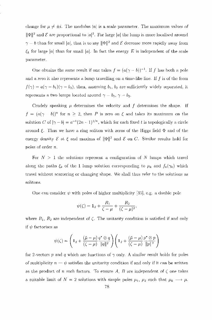
change for fL =I= ±'i. The modulus lal is a scale parameter. The maximum values of
II<PII 2 and£ are proportional to lal 2. For large lal the lump is more localised around
1 = b than for small I a I, that is to say II <P 112 and £ decrease more rapidly away from
~k for large lal than for small lal. In fact the energy E is independent of the scale
parameter.
One obtains the same result if one takes f = (a(! - b) t 1. If f has both a pole
and a zero it also represents a lump travelling on a time-like line. Iff is of the from
f(i) =a(!- bi)(i- b2 ), then, assuming b1 , b2 are sufficiently widely separated, it
represents a two lumps located around 1 = b1 , 1 = b2 .
Crudely speaking {l determines the velocity and f determines the shape. If
f = (a( 1 - b) )11 for n 2: 2, then P is zero on ~ and takes its maximum on the
solution C of h - bl = a - 1 ( 2n - 1) 1/n, which for each fixed t is topologically a circle
around ~· Thus we have a ring soliton with zeros of the Higgs field <P and of the
energy density £ at ~ and maxima of II<PII 2 and £ on C. Similar results hold for
poles of order n.
For N > 1 the solutions represent a configuration of N lumps which travel
along the paths ~k of the 1 lump solution corresponding to {lk and fk(ik) which
travel without scattering or changing shape. We shall thus refer to the solutions as
solitons.
One can consider 'tP with poles of higher multiplicity [35], e.g. a double pole
where R 1 , R2 are independent of (. The unitarity condition is satisfied if a.nd only
if ·¢ factorises as
for 2-vectors p and q which are functions of 1 only. A similar result holds for poles
of multiplicity n -1/J satisfies the unitarity condition if a.nd only if it can be written
as the product of n such factors. To ensure A, B are independent of ( one takes
a suitable limit of N = 2 solutions with simple poles p. 1 , p 2 such that P·k ~ p,.
78

Let us take 111 = f.1 + E, 112 = fl - E then ·~J is smooth in the limit E -------+ 0 only if
!1 - h -------+ 0. Writing j 1 = f + Eh, h = f - Eh and taking the limit as E -------+ 0
gives a smooth solution 4J satisfying the unitarity condition and such that A, B are
(-independent with [48, 49]
p
q
where
and
(1, f),
(1 + lfl 2 )(1, j) + (Jl-JL)g(J, -1),
g ofl OE ¢!' + h
0111 OE E=O
1 1 -(x- t) + -JL-2(x + t). 2 2
( 4.4)
(4.5)
In particular, if fl = i then ¢ = t. A number of examples have been described by
Ward [48] and loannidou [49]:
Example 4.1 If one takes fl = i, J(!) = 1 and h = 0, then the energy density£ and
II<I>II 2 are rotationally-invariant for all t. For ltl sufficiently large£ takes its maximum
value on a ring around the origin which for large ltl is of radius proportional to Jt and takes a maximum value proportional to 1/t (for small ltl it is a lump located at
the origin). The quantity II<I>II 2 is also localised around a ring for ltllarge (and again
a lump for small ltl except for t = 0 when <I> = 0). Note that at the origin, which
for each value oft is the solution of 1 = 0, II<I>II 2 is non-zero except when t = 0.
Example 4.2 If ones takes fl = i, Jh) = 1 2 and h = 0, then again II<I>II 2 and£ are
rotationally symmetric for all t. For small ltl the energy density takes its maximum
value on a ring around the origin, with the value at the origin non-zero except for
t = 0. For large ltl the energy has a. peak at the origin of height proportional to
t2 and a ring of radius proportional to t 113 and height proportional to c 2f:3 . The
situation is the same for II<I>II 2 except that <I> = 0 at t = 0.
79

Example 4.3 Perhaps the most interesting example is the scattering solution of
Ward [48]. He took p = i, f(!) = 1 and h(!) = 1 2. If r = (x2 + y2) 112 is the
radial distance, then for large r J will tend to its asymptotic value except when
g = t + ( -y + ix )2 is near to zero. Thus the solution represents two solitons at
approximately x = 0, y = ±A for t < 0 and x = ±Jt, y = 0 for t > 0. In other
words two solitons collide head on and undergo a goo scattering. More generally
one can construct N-soliton solutions which scatter through an angle of 180°/ N by
taking p. = i, f(!) = 1 and h(r) =IN·
Since one can take any rational functions f, h of 1, there are many other examples
one can construct. For example, if IL = i, f(r) = 1 2 and h(r) = 1 3, then g =
t( -y + ix) + ( -y + ·ix )3, and, as one might expect, the solution consists of a soliton
at the origin, plus two other solitons which undergo a goo scattering at the origin.
One can of course consider also higher order poles (see for example [4g]). For
example, one can take p 1 = IL + e:, {L2 = {L, {L3 = {L - e:
and h = f + e:h + e:2 k, h = f, 2 h = f- e:h + e: k.
It is clear that for a triple pole there are even more possibilities than with a double
pole.
4.2 1-Solitons
Now we shall look at solutions of the Bogomol'nyi equations in AdS2+1. We shall
start by considering the solutions obtained by the Riemann method with zeros in
Section 3.4. In particular, in this section we shall consider the N = 1 sector. We
shall write p.1 for {L, w1 for w and f 1 for f.
The N = 1 fundamental matrix solution is of the form
By analogy with the Minkowski space-time solutions we shall take f to be a rational
80

function of r2
w=x-t- . IL- (x + t)
In particular,
1 (p, + {tlfl2 (p,- {t)f)
'lj;(O) = ? -
l1tl(1 +III-) (p, -~t)f ll + Plfl 2.
vVe shall define the norm-squared of the Higgs field by II<I>II 2 = -4tr<I>2. Here it
is given by
where
and as before
llo(w) 12 p 4r411tl2
lit- (x + t)l4 P,
(4.6)
(4.7)
(4.8)
Recall from Section 3.2 that if one chooses a value p then the solution of the equation
w = c is a time-like geodesic, when Im c and Im {l have the same sign. The quantity
P is a function of w only, so it is constant on the 2-parameter family of geodesics
of the form w = c corresponding to {L. This is analogous to the quantity P in the
Minkowski space-time case which is constant on the 2-parameter family of time-like
lines in the direction determined by {l. However II<I>II 2 is not, as in the fiat case, a
constant multiple of P, since ll0 (w)l 2 is a function of the space-time variables x, r,
and t. It is though constant on the geodesics w = c. It is easily verified that on such
geodesics
llo(w )12 = 4l1ti2(Im c)2 (Im {t)2
Thus the maximum of II<I>II 2 occurs on one of these geodesics, but it is not the one
one might have expected from the Minkowski space-time case. In particular, if one
takes f(w) = a(w- b), where Imb has the same sign as Im{L, then the maximum
occurs not on w = b but on the geodesic w = c, where Re c = Reb and
81

Generally if one is given a solution in anti-deSitter space-time one can compare
its behaviour with the analogous Minkowski space-time solution. For 1-solitons the
behaviour in the curved space-time case is only approximately that of the flat case.
The best one can say is that the maximum of II<PII 2 is obtained near tow = b with
this approximation best for large Ia I, essentially because P depends on the scale
parameter lal and ll0 (w)l2 does not. \Ve shall see that this is typical of the anti
deSitter space-time solutions. Their behaviour resembles that of the Minkowski
space-time solutions and this approximation is best when the solution represents
solitons which are highly localised, in particular when we discuss behaviour described
in terms of geodesics. Intuitively we might have expected this result to hold -
the eflect of the curvature will be less over a small area and so if the solitons are
more localised the behaviour of the solution will resemble closely the behaviour
of the flat case. We shall give a more rigorous description of this idea when we
discuss zero-curvature limits. For now it is enough to note that it is useful to
consider the behaviour of our solutions in terms of their Minkowski equivalents,
even if they do not do exactly what we expect. This will be useful when we consider
the scattering solutions in Section 4.4, for example. It is also worth pointing out
that some properties carry through exactly. We shall see this when we consider for
example the N = 1 solitons with higher degree f - <P has a zero lying on the same
geodesic as for the flat case.
Example 4.4 Let us take !L = i, .f(w) = w- i. Plots of II<PII 2 are shown for various
values of t in Figure 4.1. The solution of w = i is the geodesic :r = 0, T2 = 1 + t2
,
but the maximum value of II<PII 2 is attained on w = v/2i, which is the geodesic
:r = (2v/2- 3)t, T2 = vf2 + (12v/2- 16)t2
. If one replaces f with .f(w) = a(w- i),
then the path approaches w = i as lal -------+ oo. Paths for various values of a are
shown in Figure 4.2. The argument of a aflects the shape of the soliton, but the
position depends on a only through its modulus, as in the Minkowski space-time
case. The maximum value of II<PII 2 is proportional to lal 2 and is more localised
for large lal. This is again similar to the Minkowski space-time case. 'vVe will make
considerable use of the (X, Y, s) coordinate system introduced in Section 3.2. Figure
4.3 shows plots for several values of s. The geodesic w = 'i is in fact the origin in
82

these coordinates, and so the soliton is located approximately there. One can see
that the size of the soliton in these coordinates changes with s. It is worth pointing
out that if one takes tt pure imaginary then the geodesic through the origin is the
X -axis and if tl has unit modulus then it is the Y -axis.
One might ask if there is an energy density for the .J-matrix, just as there is for
the chiral equation in the Minkowski space-time case. If we take
Pt -~rtr ((J- 1 Jt) 2 + u-!JJY + (J- 1Jr) 2),
Px -r tr ((J- 1 Jt)(J- 1 lx)),
Pr -rtr((J- 1Jt)(J- 1Jr)),
then we have
But by the properties of trace this last expression is clearly the same as
and this is of course zero for solutions of the J-matrix equation. However for the
1-solitons constructed above the integral of the energy density £ = P1 is not finite.
In fact £ does not even tend to zero at infinity for our 1-solitons - see Figure 4.4
for the case of Example 4.4.
So far we have only considered examples where f is a rational function of degree
1. We can again consider f of degree n 2': 2. Let us take f = (a(w- b)) 11 and we
shall assume that Im b and Im tl are of the same sign so that w = b is a geodesic.
Then, as in the fiat case, P has a zero on w =band takes its maximum value on the
solution C of lw- bl = lal- 1(2n -1) 1/n which again is topologically a circle around
w- b for each value oft (or s). From (4.7) it is clear that <D has a zero on w = b,
exactly as in the J'vlinkowski space-time case. The solution represents crudely a ring
soliton located around C. However this behaviour is not an exact analogue of the
fiat case, the maximum of II<DII 2 is not located on C for example, since II<DII 2 is not
a constant multiple of P. The best on can say is, as for f of degree greater than 1,
83

t = -3
40
30
20 10
0 0
t=O
30
20
10
t=3
40
30
20 10
0 0
-4
5 4
t = -2
t=2
40
3J
2J
10
Figure 4.1: Example 4.4 ~ jj<I>jj 2 for various values oft.
84
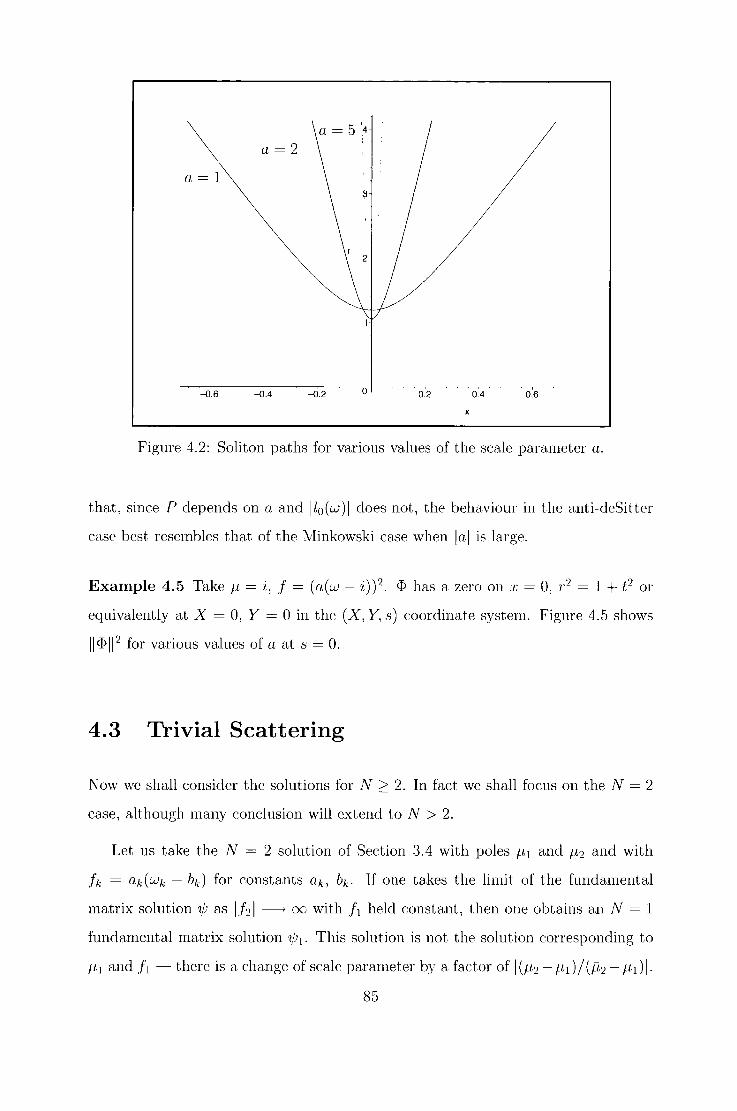
a=2
a= 1
1
-0.6 --ei.4 -0.2 0 0.2 0.4 0.6
X
Figure 4.2: Soliton paths for various values of the scale parameter a.
that, since P depends on a and ll0 (w)l does not, the behaviour in the anti-deSitter
case best resembles that of the Minkowski case when lal is large.
Example 4.5 Take {L = i, f = ( a(w - 'i) )2. <]) has a zero on :c = 0, ·r2 = 1 + t2 or
equivalently at X = 0, Y = 0 in the (X, Y, s) coordinate system. Figure 4.5 shows
II<PII 2 for various values of a at s = 0.
4.3 Trivial Scattering
Now we shall consider the solutions for N;:::: 2. In fact we shall focus on the N = 2
case, although many conclusion will extend to N > 2.
Let us take the N = 2 solution of Section 3.4 with poles {'·I and JL2 and with
.fk = ak(wk - bk) for constants ak, bk. If one takes the limit of the fundamental
matrix solution '1/J as lh I --7 oo with !I held constant, then one obtains an N = 1
fundamental matrix solution ·1/JI· This solution is not the solution corresponding to
{LJ and / 1 - there is a change of scale parameter by a factor of I (p.2- p.l) / (P·2- {Ll) I· 85

s = -1
s=O
s = 1
s = -0.7
40 3J
20
10
0
s = 0.7
40 3J
20
10
Figure 4.3: Example 4.4 - [[<I>[[ 2 for various values of s.
86

5 3
Figure 4.4: Example 4.4 - Energy density £ at t = 0.
In fact the relevant solution is fl.. = JJ.. 1 and f = ( (~t2 - JJ.. 1) / (fl2 - JJ.. 1)) j 1 . There is
a similar result of course if we hold w2 fixed and take the limit of 'ljJ as lf1 1 ----too.
Call the corresponding N = 1 solution '¢2 . Now on the geodesic w1 = c, if we let
ltl ----too (or lsi ----too), then lw2l becomes infinite and hence so does lhl- So, for
large ltl (or large lsi) , 'ljJ is given approximately by '¢1 on the geodesic. Since a similar
result holds for geodesics of the form w2 = c, it follows that the N = 2 solutions
behave like two solitons which interact without scattering. This behaviour is the
same as for the Minkowski space-time case except that the paths of the solitons are
not given exactly by wk = bk, but are close for large lakl just as in the flat case.
Example 4.6 Figure 4.6 shows the solution for fi..l = ~, JJ..2 = 2i, h = 5(w1 - i),
h = 10(w2 - i/2). Because of the choice of scale parameters the solitons are located
approximately on w1 = i and w2 = i/2 for large values of s. These paths are
respectively the origin and the X -axis. (The exact paths are w1 = J26/25i and
w2 = J13/25i).
87

a=l
a= 20
a= 500
20000
1ffi00
1rnDO
0.2
-0.2 -0.2
a= 100
4000
31lll
2000
11IIJ
-0.1 -0.1
Figure 4.5: Example 4.5 - !I<I>II 2 at s = 0 for various values of a.
88
3
0.1
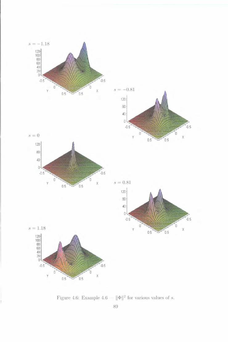
S=-1.18
120 100 80 60 40 20 0
y
s= O
120
80
40
0
s = 1.18
X s = -0.81
120
00
40
0
y
s = 0.81
120
00
40
0
Figure 4.6: Example 4.6 - II<PII 2 for various values of s.
89
X

4.4 Limiting Cases and Non~trivial Scattering
As in the Minkowski space-time case one can consider fundamental matrix solutions
with a double pole, i.e. of the form
where R 1 , R 2 are functions of w. The extension of the Minkowski-case solutions to
anti-deSitter space-time is straightforward. Again the unitarity condition is satisfied
if and only if
for 2-vectors p and q, which are functions of w only. As for the fiat case we ensure
the gauge potentia.! and Higgs field are independent of A by taking appropriate limits
of the N = 2 solutions discussed previously.
An obvious thing to try and do is to consider the anti-deSitter analogues of the
IVIinkowski space-time solution of Section 4.1. As a first attempt we consider N = 2
solution with poles at tt1 = tt + E, tt2 = p- E and take h (wl) = f(wl) + Eh(wl),
h(w2 ) = f(w 2 ) - Eh(w2 ). Then in the limit p -----t 0, exactly as in the fiat case
[48, 49],
]J (1, f),
q (1 + 1!1 2 )(1, f)+ (p,- tt)g(j, -1),
where
g 8!11 8E c=O
¢!' + h
and
aw -
8E T2
(tt - ( ~D + t) )2.
Ioanniclou has obtained this result in [45].
90
(4.9)
(4.10)
( 4.11)
(4.12)
(4.13)
( 4.14)
(4.15)

16
12
8
4
Figure 4. 7: Example 4. 7 II<PII 2 at s = o.
Example 4.7 Take tt = i, f(w) = w- i. Then II<PII 2 actually depends on x, rand
t only as a function of w and is given by
2 (Imw) 2((2 + lwl 2)2 - 8(Imw)2) II<PII =
128 ((2 + lwl2)2 + 4 Imw(2(Imw- 1)- lwl 2)2.
This gives a ring soliton with a zero of <]) on w = ,J2i and with II<PII 2 taking its
maximum on lw- 2il = J2, see Figure 4.7. One should not think of this as the
analogue of Example 4.1 as one might think at first from our choice of ft, f and h
(we shall discuss what is later). For one thing II<PII 2 is not just a function of w in
the Minkowski case - if it were it would be time independent. In particular in this
example <]) has a zero for all t (or equivalently for all s).
Ioannidou considered a similar example in [45]. She took J(w) = w, h = 0. Again
this is a function of w only. This has a zero at the solution of w = i, i.e. x = 0,
r 2 = 1 + t2. In the X, Y , s coordinate system this solution is dependent only on S
and the radial distance p = ( X 2 + Y 2)
1/2.
Example 4.8 Take tt = i, f(w) = (w- i)2. This gives a soliton with a "spike"
approximately located at w = i and surrounded by a ring-like structure (see Figures
4.8 and 4.9). It is thus similar to the Minkowski case Example 4.2 , however it too
should not be thought of as the analogous case to Example 4.2 as we shall see.
91

600 500 400 300 200 100
0 0
Figure 4.8: Example 4.8 11<1>112 at t = 0.
Perhaps the most interesting thing to attempt is to find solutions that undergo
scatterings as in the Minkowski case. It is difficult to make sense of the idea of a 90°
scattering, for example, in the (x, r, t) system. However in the (X, Y, s) coordinate
system one can make sense of it. We shall aim to construct solutions consisting of
2 or more solitons which meet at the origin at s = 0 and scatter at various angles.
By analogy with the fiat case one might expect taking !t = i, f(w) = w- i and
h(w) = (w- i) 2 might do the job. However the result is two solitons which hardly
move in the (X , Y)-plane. (One might also have expected f(w) = w, h(w) = w2 to
work but this gives even worse results). Again as in Example 4. 7 the behaviour of
the Minkowski case does not seem to go over to the anti-deSitter case, even to the
extent that the N-soliton solutions did.
The problem is in the choice of solutions whose limit is taken, or equivalently in
our choice of wk. For each singularity we could have chosen any combination of x,
r and t which is eliminated by the operators
( 4.16)
and
( 4.17)
92

400
300 200 100
0 -0.6
-0.4 -0.2 y
Figure 4.9: Example 4.8
X
II<I>II 2 at s = o.
The way we have chosen the wk they may seem to bear little resemblance to the
corresponding Minkowski space-time quantity used in Section 4.1,
However if we multiply wk by {tk then we obtain
which looks much more similar . In fact if we consider /k = /LkWk + 1 and put r = 1 +y
then for small x. y, t (i.e. to first order)
( 4.18)
which is the Minkowski space-time quantity (except for a factor of-2). In particular
when It= i one has 2i(x + iy) A better argument is to use the coordinates (X, Y, s)
coordinate system. To lowest order in X, Y, and s, x ~ 2X, r ~ 1 - 2Y, and t ~ s.
So if we express /k in terms of X, Y and s then, again to lowest order ,
which is again the Minkowski space-time quantity if we identify 2X with x, -2Y
with y and s with t (the factors of 2 occur because of our choice of coordinates in
93

the (X, Y, s) coordinate system and in particular our decision to make (X, Y) lie
within a unit disc rather than the more natural choice of a disc of radius 1/2). Both
these approximations will resurface when we consider zero-curvature limits in the
next section. All this suggests that we should use /k in place of wk to obtain solution
analogous to those in the Minkowski case.
So as before we shall take p 1 = {t + E, {t2 = JL - E but this time we replace wk
with /k, i.e. we take / 1 (II) = /(/1) + ch(/t), ,h(/2) = !(!2) - ch(/2). In the limit
p.-----> oo one obtains a similar factorisation of ·1/J(J.) with p and q and given by (4.9),
(4.10), but this time g is given by
( (x- t) + ( _:; ))2Jt-2 (:r + t)) J'(!) + h(!). 1-p. x+t
Note that again to first order ¢ is given by
(:c- t) - fL-2 (.7: + t)
or, in terms of X, Y and s,
(2X- s) -~t-2 (2X + s).
which is the same as the equivalent Minkowski space-time quantity (again with the
factor of -2), further suggesting that this is the right approach. Again in particular
when p. = i and ¢ = -2t. (Note that we could have carried out our analysis of the
1-soliton and trivial scattering solutions using /k in place of wk - the conclusions
would be the same since the set of rational functions of /k is the same as the set of
rational functions of wk - and in fact this would be the more natural approach.)
With all this one might hope that one could use this method to construct scat
tering solutions analogous to the Minkowski solutions by choosing a limit of solitons
which are highly localised by the choice of a large scale parameter. For small time
intervals around t = 0 and in a neighbourhood of :r = 0, r = 1 (or equivalently for
small time intervals around s = 0 and in a neighbourhood of X = 0, Y = 0) the
closeness of the the anti-deSitter space-time quantity 1 to its Minkowski space-time
equivalent would mean hopefully that the solitons meeting at :c = 0, r = 1 at t = 0
would scatter as in the Minkowski case, although the long-term behaviour might be
94

different. We shall see that this is indeed the case. First however we shall return to
the question of what solutions (if any) most naturally correspond in the anti-deSitter
case to Example 4.1 in the Minkowski case.
Example 4.9 Take p. = i and f(t) = wy, h(t) = 0 where we shall assume a > 0.
For s small it represents a lump located around X = 0, Y = 0. For larger values of
s the solution represents a more ring-like structure (see Figure 4.10). This mostly
resembles the Minkowski space-time case for a large as one might expect.
We now shall construct the solutions analogous to the Minkowski space-time
scattering solutions described in Section 4.1. Recall that if one chooses p, = i,
f(J) = 1 and h(t) =IN then one obtains a solution corresponding to a configuration
of N solitons which undergo a 180° IN-scattering at the origin at t = 0. More
generally if one considers f = a1, h = baN IN, then one obtains a configuration of
solitons located at points (x, y) where -y + ix given by the Nth roots of -tlb.
So we shall take ~L = i, f =a{, h = baN{N, (a, b real) for the anti-deSitter case
also. Choosing a large and considering small intervals of s, gives solutions which
undergo an approximate 180° IN-scattering at the origin, although they leave these
paths for large s. One can crudely rotate this configuration by an angle of ¢ by
replacing b with beiNB.
Example 4.10 Take N = 2, a = 4, b = 4. Figure 4.11 shows this solution. Two
solitons approach the origin roughly along the Y -axis for s < 0, begin to interact
with each other, form a ring soliton at s = 0 and then exit along the X-axis for
s > 0. Note that the paths are not exactly the axes, the solitons are not the same
height and the ring soliton is not exactly symmetric. It is however clearly similar to
the corresponding Minkowski space-time case.
Example 4.11 Take N = 3, a= 4, b = 4. Figure 4.12 shows this solution. Three
solitons approach the origin roughly at angles of 120° to each other, one along the
positive Y-axis for s < 0, begin to interact with each other, form a ring soliton at
s = 0 and then exit undergoing a 60°-scattering s > 0. As in the previous example
the behaviour is analagous to the behaviour seen in the Minkowski case.
95

a=1
30 25 20 15 10 5 0
-0.6 -0.1J2
a=5
80 60 40 20
y X
-0.4
a=2
a= 10
160
120
00
40
0 -0.4
Figure 4.10: Example 4.9 - II<I>II 2 at s = 0.64 for various values of a.
96

s = -0.1
s=O
16000
12000
fffiO
4000
s = 0.1
s = -0.04
16000
12000
8(0]
4(0]
s = 0.04
161lll
12000
BIXJJ
4[0)
Figure 4.11: 90° scattering. Example 4.10 - 11<1>11 2 for various values of s.
97

s = -0.1
6000
4000
2000
s=O
s = 0.1
8 = -0.025
6000
4000
2000
s = 0.025
6((()
4((()
2((()
Figure 4.12: 60° scattering. Example 4.11
98
II<DII 2 for various values of s.

4.5 Zero-Curvature Limit
In [20] Atiyah described the process whereby one considers families of monopole
solutions on hyperbolic spaces, one solution for each value of the scalar curvature of
the space and recovers Euclidean monopoles by taking a suitable limit as the scalar
curvature tends to zero. This is equivalent, by a rescaling argument, to taking a
family of hyperbolic monopoles on a space with a given scalar curvature but with
different boundary conditions (different asymptotic values for the Higgs field) in
each case.
In this section we shall attempt to perform the analogous process for solutions
of the Bogomol'nyi equations in the (2 + 1 )-dimensional case. One reason for doing
this is it helps explain the similarity between the behaviour of the solutions in anti
deSitter and Minkowski space-times.
There are a number of ways of carrying out this limiting process. We shall
consider two basic approaches although there are a number of variations on each of
these. One is to recover the Minkowski space-time solutions directly from the anti
deSitter solutions. This involves recovering Minkowski space-time itself as a zero
curvature limit of a family of anti-deSitter space-times. The second approach is to
consider solutions of the ASDYM on a family of regions in ultrahyperbolic space-time
which are each invariant under a !-dimensional group of "Lorentz boosts", which
converge to a solution on the whole of U which is invariant under a !-dimensional
group of translations and so corresponds to a solution of the Minkowski space-time
equations. This approach as we shall see can be viewed as a zero curvature limit and
is basically the same as the first. This is analogous to a. process described by Atiya.h
where on considers families of solutions of the ASDYM equations parameterised by
a. real number p, invariant under a. 1-dimensiona.l group of rotations in which the
invariant plane is taken to infinity along one axis
We shall start with the latter approach. We shall work with the ultra.hyperbolic
slice U1 with coordinates x, :y, t and u as in Section 3.1. For each p > 0 we
shall consider the wedge y + p > lsi, as we did (with p = 0) in Section 3.2. Take
99

coordinates
y r cosh( B)- p
u r sinh( B).
We shall look for solutions of the ASDYM which are invariant under a0 = (y +p )ay
uau (that is (w + p)aw- ('Lv- p)a1u in the double-null coordinate system). These
will of course correspond to solutions of the Bogomol'nyi equations in anti-deSitter
space-time. Note that p- 1a0 -------+au = (aw + aw) and so the limit of such a family
of solutions corresponds to a solution of the Minkowski space-time Bogomol'nyi
equations. What we shall actually do is look for fundamental matrix solutions of
the Lax pair for the ASDYM invariant under B which in a suitable limit converge
to solutions invariant under v, as in the Minkowski case, which will in turn give the
appropriate ASDYM solutions. We shall start by looking at theN-soliton solutions
and then discuss the limiting cases and scattering solutions.
The N-soliton solutions described in Section 3.4 are described in terms of an
invariant spectral parameter. To construct the required family of solutions one needs
an invariant spectral parameter which converges to (asp -------+ oo. The generalisation
of the usual invariant spectral parameter is
((w+p)+z.
If one defines v = >..jp then, asp-------+ oo, v -------+ (so we shall work vas our invariant
spectral parameter.
One can repeat the analysis of Section 3.4 with v in place of >.., and one finds
that 1/J(v) is given by (3.13) as before, but rnk are functions of
T2
wk = (x- t) - ( ) P/-lk- X+ t
Instead we shall take the rnk to depend on x, r, t as a rational function fk of
100

As functions of x, y, t and u
rk (p + y)2 _ u2
f.lk(x+t)- .( )+p p- fL~; :r + t
fLk(x- t)- p((1 + yjp) 2- (u/pf)(1- p.-1 (x + t)/p)- 1 + p
fL~;(x- t)- p((1 + yjp) 2- (u/pf)(1 + fL- 1 (x + t)jp + ... ) + p
as p -----+ oo. The fundamental matrix solution ·ljJ(v) defined with a given set of
poles ft 1 .. . fLN and rational functions f 1 ... fN converges to the usual :rviinkowski
space-time function 1/J(() described in Section 4.1 with the same fLk and f~;. To be
more precise, given a point q of 1U 1 then for each value of (, ·ljJ ( v) defines a value at
q for all p sufficiently large, and this converges (pointwise) to ·~'( (). It is also the
case that the gauge potential corresponding to ~;(v) converges to the gauge potential
corresponding to '1/J ( ().
The anti-deSitter solutions obtained as limiting cases of the N solitons described
in Section 4.4 in the zero-curvature limit give the limiting cases in the Minkowski
space-time, i.e. the two limiting processes are interchangeable. To see this, first
recall that ·1/J is given in the anti-deSitter and Minkowski cases by expressions in
volving only ~: which differ only in the definition of~~- for r--1Iinkowski space-time
we shall take
1 = p ( :r - t) - 2y - fL -I ( x + t)
(which differs by a factor of -2 from the more usual definition given in Section 4.1)
and in the anti-deSitter space-time it is
r2 1 = JL(:r- t) - , -l( ) + ]J. p-p, x+t
Second the limit of ~: in the anti-deSitter space-time case asp -----+ oo (with x, t, y
and ·u, fixed) is the corresponding Minkowski space-time quantity, since
101

This last quantity is the Minkowski space-time quantity ~Z, which shows that the
limits are interchangeable.
The second approach is to consider the solutions of the Bogomol'nyi equations
in the (2 + 1 )-dimensionaJ anti-deSitter space-time and take a suitable limit. Recall
that anti-deSitter space-time has constant curvature and scalar curvature -6. If one
replaces the metric g with p2g for some p > 0 then the scalar curvature becomes
-6jp2. The Bogomol'nyi equations are then
T D/I> = +-Ft:c·
p
If (A, <I>) is a solution for metric g, then (A, <I>/p) is a solution for metric p2g. Of
course we cannot just take take a limit of a solution (A, <I>/ p) as p ---+ oo
one obtains (A, 0), which satisfies the limiting equation Dt <I> = 0 • Fxr. There is
also the issue of recovering Minkowski space-time from the various curvature anti
deSitter space-times. The solution is first of all to consider a family of the N -solitons
parameterised by p and increase the scale parameters ak in proportion top. vVe shall
start with theN= 1 case. Since II<I>II is proportional to a= a1 this gives us a chance
that our family of solutions will converge. However the apparent size of the base of
the soliton in the AdS2+1 coordinates is proportional to 1/a, so this family will not
converge to a limit. However since the metric is proportional top the actual size of
the base tends to a constant. (One also has to make sure that the position of the
soliton is chosen in a suitable way its distance from the origin of the p solution in
the metric p2 g tends to a limit and the position in the rescaled coordinates tends to
a limit).
Now we shall describe the general case for N-solitons in detail. We take the .h
to be functions of
and choose
or more generally Jk( rk) = 9k (Prk) for rational functions 9k. One expresses the
connection A and Higgs field <I> in terms of the coordinates X, Y, s, then rescales
102

the Higgs field 1> ~ 1>/b to obtain a solution on the scalar curvature -6/p2 space
time. If one rescales the coordinates so X ~ X/2p, Y ~ Y /2p, s ~ s/p the
metric 2 2 dX2 + dY2 2 2
4p cos s (1 _ (X2 + Y2) )2 - p ds
becomes
2 cLY 2 + dY2 2
cos (s/p) (1- (X2 + Y2)jp2)2 - ds
so pointwise converges to the usual Minkowski space-time metric (identifying X with
:r: and so on). Note that by rescaling, s becomes proper time again. If we take a
limit asp ~ oo then Ax, A}', As and 1> converge to the Minkowski space-time
equivalents. In particular if one takes N = 1, f-t = i and f ( 1) = p~f, then in the limit
as p ~ oo then the connection and gauge potential converge to their Minkowski
equivalents if we take p. = i, f(!) =I· In particular
2 1 II <I> II ~ 32 (1 + 4X2 + Y2)2,
which is the value of 111>11 2 in the Minkowski case.
The two methods described are closely related, since under the isometry x ~
p:r, y ~ py, t ~ pt
r2 I = f-t( X - t) - + ]J
p -{t- 1(x + t)
becomes
p(f-t(x- t)- ~~2
( ) + 1). 1-f-L x+t
So the first method can be thought of as taking a limit as the scale parameter tends
to infinity as we did in the second method.
103

Chapter 5
Hyperbolic Monopoles
In this chapter we shall construct explicit examples of hyperbolic monopoles. Hyper
bolic monopoles are topological solitons which are Yang-Mills-Riggs configurations
on a constant curvature space H 3 with negative scalar curvature, analogous to the
monopoles described on IE3 previously. They are solutions to the Bogomol'nyi equa
tion on H 3 subject to suitable boundary conditions and are local minima of the
Yang-Mills-Riggs energy density on H 3 . Solutions of the Bogomol'nyi equations
correspond to solutions of the ASDY!vi invariant under a !-dimensional group of
rotations and so the Bogomol'nyi equations are integrable. Atiyah first considered
hyperbolic monopoles in [20] and observed that they correspond to rotationally
invariant instantons, at least when the asymptotic value of the Higgs field p is an
integer. One reason for studying hyperbolic monopoles is that they are often easier
to find and their solutions can be expressed explicitly in simple forms using ratio
nal functions. Also it was suggested by Atiyah that Euclidean solutions can be
recovered from the hyperbolic case by taking a suitable limit as the scalar curvature
tends to zero. By a. resealing argument this corresponds to taking a limit as p tends
to infinity. Some rigorous results have been established in this area by Jarvis and
Norbury [50].
vVe shall construct a number of solutions in the case p = 1/2. Apart from
the !-monopole sector which is well-known, these include a 7-parameter family of
2-monopole solutions, axially-symmetric monopoles of arbitrary charge and higher-
104

charge configuations.
5.1 Hyperbolic Monopoles and Instantons
Recall that hyperbolic 3-space is the open upper half-space
H 3 = {(x,y,r) E IR3: r > 0}
equipped with the metric
This is a manifold of constant curvature and (constant) scalar curvature -6/a2. The
geodesics are semi-circles meeting the plane r = 0 perpendicularly (along with the
limiting case of half-lines parallel to the r-axis) and has volume form
It is isometric to the ball ofradius 2a in IR3 with metric ( 1- ( 1.: 2 +:~P+ z2) / 4a2
) - 2 ( dx2+ dy2 + dz2
). In this case the geodesics are semi-circles meeting the sphere at infinity
perpendicularly with a limiting case of a straight line segment through the origin.
From now on we will concentrate on the case a = 1.
The Bogomol'nyi equation on H 3 is Dif> = -*F, where F is the curvature of a
connection A, if> is a section of the adjoint bundle, Dif> is the covariant derivative
with respect to A and * is the Hodge star relative to the metric on H 3 . Explicitly
the equation is
D if>= -TF: y rx'
Hyperbolic monopoles are solutions of the Bogomol'nyi equation subject to certain
boundary conditions, the principal one being that the asymptotic value of the norm
of the Higgs field p is a fixed positive number. Also the energy
(5.1)
105

is finite, where bracket denote the inner product and £ is energy density. The
Bogomol'nyi argument used in Section 1.1 goes through in the hyperbolic case just
as in the Euclidean case. So solutions of the Bogomol'nyi equations are local minima
of£.
In this thesis we shall deal exclusively with 5U(2) monopoles using inner prod
uct (A, B) = -(1/2) tr(AB) and its norm IIAII 2 = -(1/2)A2. The monopoles are
classified by a topological charge n given by
-1- j - tr Dei> !\ F.
47Tp .
which can be thought of as an element Ir2 (5U(2)).
Consider an anti-self-dual connection Hl on Euclidean space IE4 with curvature
G, so *G = -G, where * is defined with respect to the Euclidean metric. Recall
that instanton solutions have finite Euclidean action
that this implies that the connection extends to a bundle over the conformal com
pactification 5 4 , and instantons are classified by a topological charge which is the
second Chern class of the bundle over 5 4 and is given by
c2 = ~ j -tr(G !\G). 87T
Recall also that if x 0 , ... ,x3 are the standard coordinates on IE4 then putting x 0 = x,
:1: 1 = y and choosing polar coordinates (r, B) in the (:~: 2 , x 3 )-plane the Euclidean
metric becomes
and thus IE4 with the planer = 0 removed is conforma.lly equivalent to the product of
hyperbolic space H 3 and the circle 5 1. Atiyah observed [20] that it follows that 5 1
-
invariant ASDYM fields correspond to solutions of the Bogomol'nyi equations on H 3
and moreover that instantons correspond to finite energy solutions - we described
this reduction in Section 2.3. We (locally) choose a gauge in which the components
l1Vr, lV11 , l1Vr and H'e are independent of e and put vVx = Ax, vVy = Ay, vVr = Ar
and vVe = <T). Then F'.ry = Gxy and Dxif> = Gxe and so on. This is analogous to
106

Euclidean monopoles, which correspond to translation-invariant ASDYM fields, but
with infinite action. Recall that there is however one subtlety here not present in
the translation-invariant case. The notion of S 1-invariance of l¥ involves lifting the
S 1-action on IE4 to an action on the principal bundle on which vV is defined. If we
restrict our attention to the gauge group SU(2) work with the bundle V associated
to the fundamental representation of SU(2) we must now lift the action to one on
V. Such an action, on restriction to the planer= 0, is (up to conjugacy)
for some integer p, where a is the angle of rotation. Thus the possible lifts of the
S 1-action are classified topologically by the integer p. In fact p is the asymptotic
value of the norm of the Higgs field as r tends to zero. This is because the Higgs field
is the difference between the covariant and Lie derivatives in the () direction. From
the expressions for monopole charge n and instanton number we see immediately
that c2 = 2pn.
The strict notion of an 5 1-invariant instanton implies that p is an integer and
the instanton number is even. Nash [51] pointed out that hyperbolic monopoles
with half-integral p correspond to instantons with odd instanton number (we will
be interested especially in the case p = 1/2) and we shall also refer to these as
S 1- invariant instantons even though under a 2n rotation A is transformed to -A.
The final possibility is that p be neither integral nor half-integral. Such a monopole
corresponds to an ASDYM field which does not extend to the plane r = 0 and these
have been considered, for example, by Murray and Singer [55].
Atiyah considered integral hyperbolic monopoles and the corresponding vector
bundles, both over the full twistor space, which is ICIP3, and over minitwistor space.
The minitwistor space is ICIP1 x ICIP1 (see Sections 2.3 and 2.4). This space can be
identified with the space of oriented geodesics, with the orientation reversed by the
real structure a(A, w) = (w, 5.), which corresponds to the real structure a3 in Section
2.3. To see this, we can identify a point A E ICIP1 with the point (ReA, Im A, 0) in
the plane r = 0, and one can think of the first factor in the minitwistor space as the
107

planeT= 0 together with a point at infinity in the open upper half-plane model (or
the boundary sphere in the ball model). It is straightforward to show that a point
( )q, .-X-2) in the minitwistor space corresponds to the geodesic which meets T = 0 in
the points given by A1 and A2 using the minitwistor correspondence. Clearly the real
structure swaps the corresponding end points and so can be thought of as changing
the orientation. The points of the form (A,..\) are mapped to themselves by the
real structure, that is to say the set of such points forms the real twistor space and
corresponds to the plane T = 0 in the open upper half-space model (and of course
the boundary sphere in the ball model).
Atiyah obtained a number of results for hyperbolic monopole bundles both over
the full twistor space and over the minitwistor space. In particular the bundle E'
over minitwistor space has two splittings
where £+, .c- are line bundles equivalent to H;_p-k ® H~, H;_P ® H~p-k respec
tively, where H+ (H_) is the pull-back to CJP> 1 x CJP>1 of the Hopf line-bundle under
the projection map onto the first (second) factor of the product. (The Hopf line
bundle is the line bundle whose fibre above a point of CJP>1 is the corresponding
1-dimensional subspace of C 2). Atiyah showed that the monopole is determined by
a spectral curve as in the Euclidean case.
Atiyah also gave a rational map description of hyperbolic monopoles. One con
siders solutions of (Dp + 'i<P)s = 0 where p = logr. There are solutions S± which
are asymptotic to exp ( ±pp) as p ---> -oo and similar solutions s~ as p ---> +oo.
Writings+= as~ +bs~ one defines the rational map by f(x+'iy) = ajb. Under this
description, hyperbolic n-monopoles correspond to based rational maps of degree
n. This method involves choosing a direction in H 3, namely that of the T-axis, and
of course one could have chosen any other direction. Just as in the Euclidean case
there is a Jarvis rational map description involving fixing a point P and considering
(D 11 + ·i<P)s = 0 on lines through P with unit tangent u.
108

Nash [51] constructed examples of the 1-monopole sector explicitly using the ball
model and by taking solutions of the form
Bsinh s p = --,------
sinhBs'
Q a <I>= -xz_;;_. R 2i'
Q = ~dP P ds'
where s = 2 tanh -l R/2 is the (hyperbolic) distance from the centre of the ball
and B - 1 is (with our conventions for the norm of <I>) twice the asymptotic value
of the norm of the Higgs field. Nash also described these solutions in terms of
the corresponding instantons in the case that p is integra.l or half- integral. The
instantons can be obtained from the t'Hooft ansatz by taking 2p+ 1 equally weighted
singularities equally spaced on a circle of radius 2 around the plane of rotation. This
gives an 5 1-invariant instanton despite the fact that the solution of the Laplace
equation is not rotationally invariant. These solutions were also constructed by
Chakrabati [52] using a traditional integrable systems approach and a number a
complicated coordinate transformations.
There are a number of other papers on hyperbolic monopoles, including the
following. Braam and Austin [53] have considered integral and in particular half
integral hyperbolic monopoles as invariant instantons using the ADHM construction.
The analogue of the N ahm equation is discrete, being defined on a lattice of 2p + 1
points. They also showed that the monopole is determined by its asymptotic value
on the boundary sphere, i.e. by the restriction of the instanton connection on S 4 to
the invariant S2.
Murray and Singer [55] generalised the twistor description to non-integral p show
ing that hyperbolic monopoles correspond to bundles over a twistor space which is
OP 1 x ClP 1 minus the diagonal corresponding to the real twistor space. They gener
alised some of Atiyah's results for integral p, namely the existence of two splittings
for the monopole bundle and the fact that the monopole is determined by its spectral
curve.
Jarvis and Norbury [50] showed that the limit of the Jarvis rational map for
109

hyperbolic monopoles is the Jarvis map for Euclidean monopoles.
Sutcliffe and Ioannidou [54] have constructed some interesting solutions for higher
gauge groups.
5.2 An Ansatz for Hyperbolic Monopoles
In this section we will construct an ansatz for hyperbolic monopoles in the case
p = 1/2, by considering the corresponding instantons. We saw in Section 2.5 that in
general the problem of constructing instantons is a difficult one. The simplest and
best-known class of solutions is that of solutions obtained from the t 'Hooft ansatz
Here the a 1w are multiples of Pauli matrices, satisfying cr !IV
self-dual (i.e. alii/= (1/2)Eilvdai\A). Explicitly we shall take
crm CJ23 1 2CJ3,
cro2 -CJ13 l
-2cr2,
CJo3 C!t2 1 2CJl.
(5.2)
-cr v 11., which are
(5.3)
The gauge potential satisfies the ASDYM equation if ¢ satisfies Laplace's equation
on IE4. To get the correct boundary conditions ¢ is of the form
(5.4)
where x 0 ... Xc 2 are (distinct) points in IE4 and J\0 ... Ac2 are positive real numbers
and lxl is distance in IE4. As a special case we may choose one of the singularities
to be the point at infinity
(5.5)
A 1-monopole corresponds to an instanton of topological charge 2p. To construct
such an instanton Nash [51] suggested using the t 'Hooft ansatz and choosing the
2p + 1 singularities to be equally spaced on the circle :z: = 0, y = 0, r = 2.
110

Instead we shall restrict our attention to the case p = 1/2. To construct the
corresponding instanton we assume that the singularities of ¢ all lie in the plane
T = 0 (including the special case that one of the singularities is at infinity). Thus
the derivative ¢0 = 0. This idea was suggested by Chakrabati in [52].
vVe shall use letters i, j, k and so on taking values 1, 2, 3 to label coordinates x,
y, T. Thus vV3 will refer to Hlr in this context. The t'Hooft ansatz becomes
i = 1, 2, 3
where L is log¢, L; refers to the derivative in the i-direction,
and a'3 = a3 . If g = exp !JiB, then under the gauge transformation corresponding to
g
{=1,2,3
and
(Again this transformation appears in [52].) If we put lVo = <I>' wi = A and Tj = ~~ '
then we obtain the ansatz
i = 1,2,3
In polar coordinates the (Laplace) equation for ¢ is
1 cPxx + c/Jyy + c/Jrr + -;:c/Jr = 0
or in terms of L
1 2 2 2 L,rx + Lyy + L,.,. + -:;.Lr + (Lx + Lv + Lr) = 0.
111
(5.6)
(5.7)

Notice that this implies that
where D. is the Laplacian on H 3.
5.3 1-Monopole Solutions
In this section the 1-monopole solutions are constructed using the ansatz above. To
do this ¢> must have two singularities. Take one singularity in ¢> to be at oo and
one in the plane r = 0. By performing a translation we can assume that the second
singularity is at x = 0, :y = 0. In other words
Then the gauge potential is
A = 2AEijkXjTk 2 (x2 + y2 + r2 + >..)(:r2 + y2 + r2)'
and the Higgs field is
The square of the norm of the Higgs field is
1 A.r2
4 (::r;2+y2+r2+)..)2' (5.8)
and the energy density £ is
(5.9)
The definition of the position of a monopoles is usually taken to be where the
Higgs field vanishes, and here this happens at :r = 0, y = 0 and r = v'>:. Note that
the energy takes its maximum value there also. As ,. tends to infinity the norm of
112

3
2 . 5
2
r1 . 5
0 . 5
0 - 2 - 2
- 1 - 1
2 2
Figure 5.1: A monopole of charge 1.
the Higgs tends to 1/2 as expected. Figme 5.1 shows a plot of a surface of constant
energy for a 1-monopole (in the upper half-space model). Of comse this solution is
the analogue of the Euclidean 1-monopole.
An alternative is to take both singularities in the plane r = 0. Let
A 1 ¢= +------
(x + a) 2 + y 2 + r 2 (x- a)2 + y 2 + r 2 · (5.10)
Then we obtain a 1-monopole at x = a(-1 + A)/(1 +A), y = 0, r = 2a.J\/(1 +A).
Notice that in both cases the zero of the monopole lies on the geodesic joining the
two singularities, r = 0 in the first case and x2 + 1·2 = a2 in the second. The position
on this geodesic is determined by the weight A.
5.4 2-Monopole Solutions
Consider ¢ of the form
¢=1+ A + ~ (x - a)2 + y2 + r 2 (z + a)2 + y2 + r-2
(5.11)
For the most we will be concerned with the case A = tt. There are 3 rnaiu possibili
ties.
113

For large a this represents two monopoles at approximately x = a, y = 0, T = J>. and x = -a, y = 0, T = J>. (or more generally T = fo), see the first plot of Figure
5.2. As a2 approaches A/ 4 the monopoles begin to interact with each other and this
description begins to break down (Plot ii).
The Higgs field has a double zero at :r = 0, y = 0, r 2 = 3A/ 4. This is the analogue
of the charge 2 solution of Ward [25] described in Example 2.4 (Plot iii).
In this case the Higgs field has 2 zeros lying on the r-axis at
r = V -a2 +A± J -4Aa2 + A2
(see Plots iv and v). Notice that although one monopole looks much larger than
the other this is due to the factor of 1·-3 in the volume form. Rotating this solution
in the (x, y)-plane gives a 1-parameter family of gauge inequivalent solutions, all
with the same zeros. This is the same as the Euclidean case, where, for a choice
of the two positions of the zeros of the Higgs field, there is again a family of gauge
inequivalent solutions parameterised by a relative internal phase. i\tloreover we can
apply isometries to a family of solutions parameterised by the distance between the
two monopoles (including the two monopole solution). I believe this generates the
whole 2-monopole space, but this requires some proof.
We could of course take all 3 singularities away from infinity in the plane T = 0.
Particularly interesting is to take the singularities to be the vertices of an equilateral
triangle:
1 ~--~~~--~+ (x- a)2 + u2 + r2
1 1
(:r + ~a)2 + (u- ~a)2 + r 2 + (:r + ~a)2 + (y + ~a) 2 + r 2 ·
If p is radial distance in the xy-plane, then

Plot
Plot u
Plot 111
-Plot IV
•
Plot v
Figure 5.2: A number of 2-monopole solutions.
115

and
-1 -0.8
-0.6 -0.4
-0.2
Y0o.2
0.4 0.6
0.8
Ox 0.2
0.4 0.6
0.8
-1 -0.8
-0.6 -0.4
--Q.2
Figure 5.3: An axially-symmetric monopole of charge 2.
£ = a4r 4 (27 K+ 4 - 12K+ 3 K_ - 14K~K-:_ - 12K+K-3 + 27 K_ 4 )
K+4K_4 '
where K± = (r2 + a 2 ± ap + p2). This solution is again the hyperbolic version of
Ward's toroidal 2-monopole solution and is shown in Figure 5.3.
5.5 Higher-charge Monopoles
By analogy with Euclidean monopoles we expect the moduli space of hyperbolic
monopoles of charge n to be a ( 4n - 1 )-manifold. Since the ansatz of Section 5. 2
has 3n + 2 parameters and thus we can hope at best to use it to construct the 1-
monopole, 2-monopole and possibly 3-monopole sectors, but in general the problem
of finding the data for a given monopole seems intractable. However we can still use
our ansatz to find a number of interesting solutions.
We may generalise the construction of the previous section and choose n + 1
singularities (n > 1) equally spaced on the circle r = 0, p = a and with equal
weights. This represents a charge-n torus, analogous to the solution of Prasad and
Rossi [26], whose Higgs field has one n-fold zero on the r-axis at r = a. For example,
116

if
1.4
1.2
.0-8 0 .6
0.4
0 .2
0 -1.2
-1 -0.8
-0.6 -0.4
-0.2
Y<(,_2 0.4
0.6 0.8
-1 -0.8
-0.6 -0.4
- 0 .2
o.2x 0.4
0 .6 0.8
-1.2
Figure 5.4: An axially-symmetric monopole of charge 3.
1 1 ~--~-------+ + (x- a)2 + y2 + r2 (x + a)2 + y2 + r2
1 1
x2 + (y- a)2 + r2 + x2 + (y + a)2 + r2'
then this is a charge 3 torus whose Higgs field has its zero on the r- axis at r = a
(Figure 5.4), and
JJ<I>JJ2 = ~- 4a2r2(J(+ 2- 2](+](- + 5](_ 2)(5K~- 2K+J(- + ](_ 2) 4 (K+ + IC)2(J(+ 2 _ 6K+K- + ](_ 2)2
One final solution is to take
¢ = 1
1+ + (x- a)2 + y2 + r2 1 1
(x + ~a) 2 + (y- v?a)2 + r 2 + (x + ~a) 2 + (y + v?a)2 + r 2.
For a 2 < 3>../8 this represents a configuration of a toroidal 2-monopole and a 1-
monopole (Figure 5.5).
117
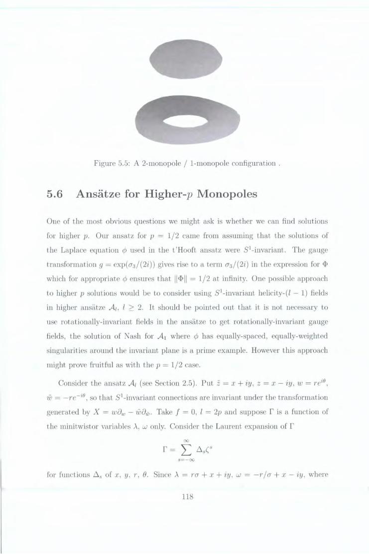
Figure 5.5: A 2-monopole / 1-monopole configuration .
5.6 Ansatze for Higher-p Monopoles
One of the most obvious questions we might ask is whether we can find solutions
for higher p. Our ansatz for p = 1/2 came from assuming that the solutions of
the Laplace equation ¢ used in the t'Hooft ansatz were 5 1-invariant. The gauge
transformation g = exp(o-3 / (2i)) gives rise to a term a3 / (2i) in the expression for {[:1
which for appropriate ¢ensures that JJC[>JJ = 1/2 at infinity. One possible approach
to higher p solutions would be to consider using 5 1-invariant helicity-(l- 1) fields
in higher ansatze At, l 2:: 2. It should be pointed out that it is not necessary to
use rotationally-invariant fields in the ansatze to get rotationally-invariant gauge
fields, the solution of Nash for A1 where ¢ has equally-spaced, equally-weighted
singularities around the invariant plane is a prime example. However this approach
might prove fruitful as with the p = 1/2 case.
Consider the ansatz At (see Section 2.5). Put z = x + iy, z = x- iy, w = rei8,
w = -re-i8 , so that 5 1-invariant connections are invariant under the transformation
generated by X =WOw- WOw· Take f = 0, l = 2p and suppose r is a function of
the minitwistor variables A, w only. Consider the Laurent expansion of r 00
S=-00
for functions !::..s of x, y, r, e. Since A= ra + T + iy, w = -r/a + T- iy, where
118
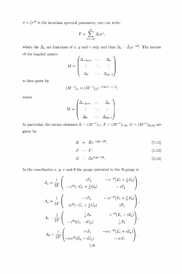
CJ = ( ei0 is the invariant spectral parameter, one can write
00
s=-oo
where the Lis are functions of :r, :y and T only and thus 6 8 = Lise- 180 . The inverse
of the banded matrix
Nf =
is then given by
where
Li-2p+i 6o
]Vf =
6o 62p-l
In particular the corner elements E = ( J\1- 1) n, F = ( J\1- 1 h.2p, G = ( NJ- 1 )2p,2p are
given by
E .Ee-i(2p-l)e
' (5.12)
F F, (5.13)
G Gei(2p-l)e_ (5.14)
In the coordinates x, y, T and (} the gauge potential in the R-gauge is
1 ( iFu Ax=-
2F 0 1 ) - e2 (-G. + .,....Go 1 l.T
1 ( - iF1:
Ay=-2F iei0 ( -G + lG ) r u· 0
Ar = -1
( 2F iO(G ·c ) -e :r-'l Y

Using (5.12) to (5.14) and applying the gauge transformation with g = exp (pCJ3/(2i))
these become
and
1 ( A:r:= 2F iFy
c.+ 2p-lc I r
A __ 1 Y- 2F (
-iFx
,.c-· ·2p-lc--t r- },-,-.
-E + 2p-l E) r r
' -iFy
,.E ,-2p-l E) -t r + l-r-' iFx
If we take the reality condition r = rt' i.e. r( .>., w) = r(\, w)' so that
- - - 2 1-then if we assume that 2p is odd then F is real and E = G. If we put E-~ E =
r
P + iQ and G + 2P1~ 1 G = P- iQ for P, Q real then we obtain
iFy iPr iQr 2F CJ3 + 2F CJ2 - 2F CJ 1'
iFx iPr iQr -(]'3 - -(]'2 - -(Jl· 2F 2F 2F ,
Ar iQx + iPv ifT - iQy CJ
2F (]'1 - 2F 2 '
1 (rFr ) PT- Qy Px + Qy Ae = - - - p CJ3 - r CJ1 - r CJ2 . 2 T 2F 2F
After putting A0 = <I> we have ansiitze for SU(2)-valued for the Bogomol'nyi equa
tions in H 3. If the derivatives of F, P and Q decay sufficiently rapidly then this
solution will have asymptotic Higgs p. In particular when p = 1/2 we recover the
original ansatz presented in Section 5.2. So far however I have been unable to find
solutions for p > 1/2.
120

Chapter 6
Outlook
In this thesis we have seen that the Bogomol'nyi equations on constant curvature
space-time are integrable and constructed a number of solutions. The methods of
solution have involved a number of interesting concepts and methods from many
branches of mathematics, especially geometry. VVe have seen that much of the
results for the fiat cases extend to the curved cases, and that, in the case of anti
deSitter space-time, as for hyperbolic space, one can recover the fiat case as a zero
curvature limit. The solutions we have constructed display a number of attractive
3-dimensional soliton solutions in the case of hyperbolic monopoles. In the anti
deSitter case there are many interesting solutions including solitons undergoing non
trivial scattering.
A number of further problems suggest themselves. In the anti-cleSitter case one
can construct a number of further solutions including higher poles. Ioannidou has
also constructed some soliton-antisoliton solutions and more work could be clone
here. It would be interesting to see if one could construct a better "energy density"
than the one constructed in this thesis, one whose integral was finite, perhaps using
·lj; ().. = 0) -l in place of our J- matrix. It would also be interesting to consider
alternative coordinate systems. In particular one could consider a coordinate system
with 2 spatial coordinates and a proper time coordinate such that all geodesics
corresponding to ~t = i represent points in space static with respect to the time
coordinate, just as we have with Minkowski space-time.
121

We have not constructed solutions in the deSitter space-time although some have
been constructed by Kotecha [57]. There is room for much more investigation into
this case. In particular the zero curvature limit and non-trivial scatterings.
In the case of hyperbolic monopoles on might try to generalise the solutions
here to higher half-integral p or to general values of p. One can also look at the
zero-curvature limit and try to recover well-known or new Euclidean monopole con
figurations. One could also try to relate the solutions to other monopoles methods
-bundles over minitwistor space, spectral curves, N ahm (Braam-Austin) equations
and rational maps.
Beyond the Bogomol'nyi equations, there are many other integrable systems,
soliton phenomena and other questions of nonlinear science which one can address.
In particular, there are many more equations obtainable from the ASDYM equations
and their generalisations which can be studied.
122

Appendix A
Vector Bundles and Connections
This appendix gathers the basic definitions of vectors bundles, connections and
curvature which are used throughout this thesis. This material is discussed in more
detail in [1], [2], [3] and [4].
A.l Vector Bundles
A smooth, rank-k, real vector b'undle over a. smooth manifold A1 is a smooth manifold
E, together with a. smooth map 1r : E ----> ]\
is mapped to (:r, Yf3o:V) for matrix valued functions 9{3o: on Uo: n U0 called transition
matrices. On Uo: n U0 n U1 the matrices satisfy
(A.l)
Conversely, to define a vector bundle it is enough to give an open cover of lvf and
transition matrices satisfying ( A.l). If the matrices can be chosen to lie in a subgroup
G of GL(n, C), then G is said to be the structure group of E.
A section of E is a map s : l\1 ~ E satisfying JT o s = idl\l· If s is instead
defined only on an open subset of l\1 it a local section and we denote by r(J\!1, E)
the set of sections of E. One can find local sections ( e 1, ••• , ek) which are linearly
independent at each point. Such a choice of sections is called a frame. Given a local
trivialisation ho: there is an obvious choice of frame, namely the one consisting of
the sections corresponding to the standard basis in Ck. If ( e1 , ... , ek) is a frame on
Uo:, (e1 , ... , ek) is a frame on U0 and g = 9f3o: is the transition matrix then
A section s is then given locally by s = sPep = sPep with
(A.2)
Conversely, to define a (global) section of E it is enough to give functions {sP} on
each open set of the cover satisfying (A.2).
If E has extra structure, then one can reduce the structure group G of E to a
proper subgroup of GL(n, C). For example if E has a Hermitian structure (in other
words a Hermitian inner product on each fibre) then we can take G to be U(k) by
replacing frames with orthonormal ones by a Gram-Schmidt process.
Given vector bundles E, F, one can construct other bundles analogous to the
various operations on vector spaces. For example, one can find the dual bundle E*
whose fibre at X is the dual space E; of E:c, the direct sum and tensor product
bundles E EB F and E 0 F whose fibres are Ex EB F.1: and Ex 0 Fx respectively and
the homomorphism bundle Hom(E, F) whose fibre is the set of homomorphisms
Hom( Ex, Fx) from Ex to P.r.- In particular, one can form the endomorphism bundle
124

End(E) = Hom(E, E) which is isomorphic toE@ E*. One can also consider sym
metric and anti-symmetric tensor products to obtain the symmetric tensor bundles
c-JP E, exterior product bundles /\P E and the exterior a.lgebra bundle 1\ *E.
The tangent bundle, the collection of tangent spaces at each point of a manifold,
is an important example of a vector bundle. One can consider the tensor algebra of
bundles obtained from T !vi, especially the cotangent bundle T* J\1 and its exterior
product 1\P(JVI) = 1\P T* !VI. Sections of 1\P(M) are called p-forms and the set of
p-forms f(J\,1, 1\P(JVJ)) is denoted DP(!VI). One can form the tensor product bundle
E@ 1\P (!VI) and consider its sections, the set of which r( J1..1, E@ 1\P ( J1..1)) is denoted
flP(E). Such a section w E flP(E) is called an E-va.lued p-form and takes vector
fields X 1, ••• , Xp to a section of E.
One final bundle construction is the pullback bundle. Given manifolds J1..1, N, a
smooth map f : Jl.1 ------+ N and a bundle E over N, one can obtain a bundle f* E
over Jl.1, called the pullback bundle, whose fibre at x is Ef(x) and whose transition
matrices ho.f3 for the cover {.f- 1(Ua) :a E A} are given by haf3(x) = 9aaU(:c)). In
particular, if 1'1 is a submanifold of N and i : Jl.1 ------+ N is the inclusion map then
i* E is the restriction of E to Af denoted EIJI.I·
A.2 Principal Bundles, Associated Bundles and
the Adjoint Bundle
A principal bundle is an object analogous to a vector bundle whose fibre at a point
:T is a Lie group G (which we shall assume is a subgroup of G L( k:, C)) instead of
a vector space. More precisely, a principal bundle over Jl.1 is a smooth manifold P
together with a smooth map 1r : P ------+ Jl.1 such that the fibres Px = n-1(:r) have
the structure of a Lie group isomorphic to G. P has an open cover {Ua : a E A}
and diffeomorphisms (local trivialisations) ho. : n-1 (Ua) ------+ Ua x G. Under the
maps hf3 0 h-;; 1 : Ua n Ua X G -------7 UQ n uf3 X G, (x, J1..1) is mapped to (x, 9(3aJ1..1) for
G-valued functions. Given a vector bundle E one can obtain a principal GL(k:, C)
bundle with the same transition matrices. If E has structure group G then one can
125

obviously form a principal G bundle.
Suppose one has a principal G bundle. Given a vector space V and a represen
tation p : G ----> G L(V) of G one can define a bundle in a similar way as we did
for vector and principal bundles by patching (:r, v) to (:r, p(g13a)v). Such a bundle
is an called an associated bundle and of course has fibre V. The most important
examples for us are obtained by the fundamental and adjoint representations.
In the fundamental representation of a subgroup G of G L( k, C) the elements of
G act on column k:-vectors by left multiplication, i.e. p(g )v = gv. The associated
bundle is just the vector bundle with transition matrices 9!3a·
If G is a Lie group with Lie algebra g, then for each g E G one can define
a map Ad9 E GL(g) by Ad9 (T) = gTg- 1. The associated bundle given by the
representation g ----> Ad9 is called the adjoint bundle. If Pis obtained from a vector
bundle E, we shall denote the adjoint bundle by adj(E). The bundle is patched by
mapping (x, T) to (x, 9!3aT9,6L~ ).
A.3 Connections and Curvature
A connection D on a vector bundle E over ll1 is a map
in other words taking sections of E to E-valued 1-forrns, satisfying
D(f · s) = f · Ds + df · s.
Given a vector field X, on can define the covariant derivative
in the direction X given by interior multiplication D xs = X .JDs.
If we choose a frame ( e 1 ••• ek) then with respect to this frame
Ds = ds +As
126

for a g[(k, C)-valued 1-form A. If {xll} are coordinates on .M, A
Ds = D11 s dx11 , then
If a second frame (e1 ... ek) frame satisfies eP = e17 g;, then with respect to the second
frame D = d +A, where A = g- 1 Ag + g- 1dg. If E has trivialisations such that one
can reduce the structure group to a Lie group G, one can consider connections D
such that with respect to these trivialisations A takes values the Lie algebra g of
G. For example, when E has an Hermitian structure ( · , · ) and one can take G to
be U(k) by choosing an orthonormal frame then A is u(k)-valued if Dis compatible
with the Hermitian structure in the sense that
d ( s, t) = ( D s, t) + ( s, Dt) .
One can extend D top-forms by D(s 0 w) = Ds 1\ w + s 0 dw for wE 0.P(J..1) and
s E f(J..1, E). Locally D is given by Dw = dw +A 1\ w.
Thus one can consider the curvature F of the connection D given by
Locally the curvature is given by D 2 s = (dA +A 1\ A) 1\ s, so it does not involve
derivatives and F E D2 (Encl(E)), i.e. an (End(E))-valued 2-form. In fact F takes
values in the adjoint bundle adj (E). For vectors X and Y, F is given by
F(X, Y) = DxDys- DyDxs- D[x,YJ·
Locally the curvature is given by F = ~ F!lvdxll 1\ dxv, where
and with respect to a second frame F = g- 1 Fg.
Given a connection D on a vector bundle E one can define a connection on the
adjoint bundle Encl(E) which is given locally by
Ds = ds + [A, s ].
127

In particular we can apply D to F. The connection satisfies the Bianchi identity
DF=O.
Finally, we can consider the pullback bundle J* E of a bundle with connection
D. One can define a pullback connection by J* D = d + J* A, where J* A is the usual
pullback of forms.
128

Bibliography
[1] L. J. Mason and N.M.J. Woodhouse, Integrab'il'ity, Self-Duality and Twisto1·
Theory, OUP (1996).
[2] R. S. vVard and R. 0. Wells, Twistor Geometry and Field Theor·y, CUP (1990).
[3] C. Nash and S. Sen, Topology and Geometry for Physicists, Academic Press,
London (1983).
[4] C. M. Nakahara, Geometry, Topology and Physics, lOP (1990).
[5] L. H. Ryder, Quantum Pield Theory, CUP (1985).
[6] R. J. Rajaraman, Solitons and Instantons, North Holland, Amsterdam (1982).
[7] M. F. Atiyah and N. J. Hitchin, The Geometry and Dynamics of Magnetic
Monopoles, Princeton University Press (1988).
[8] P. M. Sutcliffe, Int. Journal Modem Phys. A12, 4663-4706 (1997).
[9] K K. Uhlenbeck, Comm. Math. Phys. 83, 11-27 (1982).
[10] M. F. Atiyah, N.J. Hitchin and I. M. Singer, Proc. Royal Soc. A362, 425-461
(1978).
[11] A. Jaffe and C. Taubes, Vortices and Monopoles, Birkhauser, Boston (1980).
[12] E. B. Bogomol'nyi, Sov. J. Nucl. Phys. 24, 449 (1978).
[13] M. K. Prasad and C. M. Sommerfield, Phys. Rev. Lett. 35, 760-762 (1975).
[14] E . .J. Weinberg, Phys. Rev. D20, 936-944 (1979).
129

[15] R. S. Ward, Phil. Trans. Royal Society A315, 451-457 (1985).
[16] M. J. Ablowitz and P. A. Clarkson, Soldons, Nonlinear Evolution Equat'ion
and Inverse Scattering, London Mathematical Society Note Series 149 (1991).
[17] R. Penrose, J. Math. Phys. 8, 345-366 (1967).
[18] R. Penrose and vV. Rindler, Spinors and Space-time Vol. I, CUP (1984),
Spinor's and Space-time Vol. II, CUP (1986).
[19] R. S. Ward, Phys. Lett. 61A, 81-82 (1977).
[20] 1vi. F. Atiyah, lVIagnetic monopoles in hyperbolic space, Proc. Bombay Collo
quium 1984 on Vectm' Bundles on Algebraic Varieties, 1-33, OUP (1987).
[21] N. J. Hitchin, Comm. Math. Phys. 83, 579-602 (1982).
[22] N. J. Hitchin, Complex manifolds and Einstein's equations, in Twistor Geom
etr·y and Nonlinear systems, Lecture notes in Mathematics 970, 73-99 (1982).
[23] P. E. Jones and K. P. Tod, Classical and Q·uant·am Gmvity 2, 565-577 (1985).
[24] K. Kodaira, Ann. Math. 84, 146-162 (1962).
[25] R. S. Ward, Comm. Math. Phys. 79, 317-325 (1981).
[26] M. K. Prasad and P. Rossi, Phys. Rev. Lett. 46, 806-809 (1981).
[27] P. Forgacs, Z. Horvath and L. Palla, Phys. Lett. 99B, 232 (1981).
[28] R. S. Ward, Phys. Lett. 102B, 136 (1981).
[29] E. Corrigan and P. Goddard, Cmnm. Math. Phys. 80, 575-589 (1981).
[30] S. K. Donaldson, Comm. Math. Phys. 96, 387-407 (1984).
[31] J. Hurtubise, Comm. Math. Phys. 100, 191-196 (1985).
[32] vV. Nahm, The construction of all monopoles by the ADHM method, in
Monopoles in Quantum Field Theory, World Scientific, 87-94 (1982).
130

[33] N. J. Hitchin, Comm. Math. Phys. 83, 145-190 (1983).
[34] N. J. Hitchin, N. S. Manton and M. K. Murray, 661-692 (1995).
[35] R. S. Ward, J. Math. Phys. 29, 386-389 (1988).
[36] R. S. Ward, J. Math Phys. 30, 2246-2251 (1989).
[37] R. S. Ward, Co'mm. Math. Phys. 128, 319-332 (1990).
[38] R. S. \Nard, Twistors, Geometry and Integrable Systems, in The Geornetric
Universe, eels S. A. Huggett et al, OUP, (1998).
[39] S. W. Hawking and G. R. Ellis, The Large Scale Stmctu:re of Space-time, CUP
(1973).
[40] R. S. vVard, Asian J. Math. 3, 325-332 (1999).
[41] V. E. Zakharov and A. B. Shabat, Functional Analysis Appl. 8, 226-35 (1974).
[42] V. E. Zakharov and A. B. Shabat, Functional Analysis Appl. 13, 166-73 (1976).
[43] Zixiang Zhou, J. Math. Phys. 42, 1085-1099 (2001).
[44] Zixiang Zhou, J. Math. Phys. 42, 4938-4947 (2001).
[45] T. Ioannidou, Nonhneraity 15, 1489-1497 (2002).
[46] T. Ioanniclou, Int. J. Mod. Phys., 18 4975-4998 (2003).
[47] T. Ioanniclou, Theor. Math. Phys 137, 1472-1475 (2003).
[48] R. S. \,Yard, Phys. Lett. 208A, 203-208 (1995).
[49] T. loannidou, PhD Thesis, University of Durham (1996).
[50] S. Jarvis and P. Norbury, B1tlletin of the LMS 29, 737-744 (1997).
[51] C. Nash, J. Math. Phys. 27, 2160-2164 (1986).
[52] A. Chakrabati, J. Math. Phys. 27, 340-347 (1984).
131

[53] P. J. Braam and D. M. Austin, Nonlinearity 3, 809-823 (1990).
[54] T. Ioannidou and P. M. Sutcliffe, J. Math. Phys. 40, 5440-5455 (1999).
[55] M. Murray and M. Singer, Nonlinearity 9, 973-997 (1996) .
[56] R. Jackiw, C. Nohl and C. Rebbi, Phys. Rev. D15, 189-192 (1977).
[57] V. Kotecha, J. Math. Phys. 42, 1018-1025 (2001).
132