Economic Abuse: A Theory of Intrahousehold Sabotage✩

Dan Anderberg

Royal Holloway University of London, Institute for Fiscal Studies

Helmut Rainer

University of Munich, CESifo, Ifo Institute for Economic Research

Abstract

While research on domestic abuse in economics has to date almost exclusively focused on physicalviolence, research in other disciplines has documented that abusive males frequently also use sab-otage tactics to interfere with the employability and job performance of the victim. This paperputs forward a theoretical framework that rationalizes why men may use labor market sabotage“instrumentally” to thwart their partners’ training or career efforts. The model predicts a non-monotonic relationship between the gender wage gap and intrahoushold sabotage committed byabusive males. There are no one-size-fit-all solutions when it comes to reducing the incidence ofeconomic abuse. Instead, specific measures have to be targeted at different types of households.

Keywords: Economic abuse, intrahousehold sabotage, non-cooperative family decision-making,welfare policy.JEL Classification: J12, J22, D19.

1. Introduction

The term domestic abuse typically evokes images of physical and sexual violence. However,researchers across a range of social science disciplines have long understood that a typical patternof domestic abuse also includes economic abuse as a tactic used by perpetrators to control theirpartners’ behavior (Tjaden and Thoennes, 1998). Economic abuse consists, inter alia, of sabotageactions that act as barriers to the employability and job performance of the victim (Swanberg andMacke, 2006; Adams et al., 2008).1 For example, there is evidence of abusers starting fights andkeeping their partners up all night before an important job interview or test. Others are disruptingtheir partner’s work effort or try to damage their reputation at work. Some perpetrators sabotagetheir partner’s child care arrangements etc. The various tactics used by abusers share the common

✩Earlier versions of this paper were presented at the Geary Institute, FEDEA Madrid, EEA in Malaga, CESifoArea Conference on Employment and Social Protection, University College Dublin, and at the Universities of Munich,Konstanz and St Gallen. We are grateful to participants for their comments.

Email addresses: Dan.Anderberg@rhul.ac.uk (Dan Anderberg), rainer@ifo.de (Helmut Rainer)1Indeed, the so-called Work/School Abuse Scale (W/SAS) survey instrument was constructed to measure inter-

ference with employment and education by abusive males (Riger et al., 2000).

Preprint submitted to Elsevier September 6, 2012

feature that they thwart the victim’s work or training efforts, in some cases through direct physicalviolence.2

Economic abuse has so far remained a relatively “unseen side” of domestic violence. Indeed,recent research in economics on the causes of domestic violence has focused mainly on physicalabuse. The most commonly used framework, which builds on the cooperative approach, assumesthat some males have a preference for physical violence and women tolerate it in return for highertransfers (Tauchen et al., 1991; Farmer and Thiefenthaler, 1997; Aizer, 2010).3 While this literaturehas been insightful, no attempt has yet been made to understand intrahousehold economic abuse.In particular, no explanation has been put forward regarding what might drive husbands who, astheir wives enter employment or increase hours of work, turn into saboteurs and contrive to pullthem back down. With this paper, we aim to fill this void by presenting a theory of intrahouseholdsabotage which rationalizes economically abusive behavior within partnerships.4

The key feature of our analysis is to think of economically abusive behavior as emerging en-dogenously from the internal organization of the family. More specifically, our theory is predicatedon the idea that incentives for sabotage are a consequence of spousal disagreements regardingtheir respective economic roles, modeled here as having its root cause in the time allocated tothe provision of family-specific public goods. To this effect, we present a model which depictsfamily behavior as a noncooperative game. However, we also assume that partners have caringpreferences, which implies that, for couples with “near complete caring”, equilibrium behavior isnearly “completely cooperative”. Hence the caring parameter effectively parameterizes the degreeof noncooperation. In the model, each partner derives utility from own private consumption andfrom a household public good which is produced using time-inputs by both partners. In the non-cooperative equilibrium, spouses do not provide the efficient level of the family public good, andeach partner would like the other to work less in the labor market and to contribute more timeto household production activities. We allow for transfers between the partners. Transfers servetwo purposes. First, a partner may use a transfer to support the other’s consumption. Second, atransfer by one partner may also serve the purpose of influencing the other’s time allocation.

The only gender asymmetry in the model is that men are assumed to have the option of usingeconomically abusive behavior. A motivating fact for this assumption is that most victims ofdomestic violence in general and economic abuse in particular are women. Economic abuse in ourmodel is an instrumental activity that is directly targeted at women’s labor market opportunities.This modeling approach is motivated by the observation, outlined in detail below, that abusivemales routinely sabotage their partner’s labor market activities. In particular, we will identifyinstrumental incentives for economic abuse with the husband’s equilibrium utility being locallydecreasing in the wife’s earnings capacity. We assume that, by behaving economically abusive, thehusband can damage his partner’s earnings capacity through direct and indirect interference withwork efforts.

2According to the literature, the examples highlighted above are repeatedly reported by victims of domesticviolence (see, e.g., Johnson, 1995; Brandwein and Filiano, 2000; Raphael and Tolman, 2000; Swanberg and Logan,2004; Swanberg and Macke, 2006)

3Others have argued that intimate partner violence represents expressive behavior that is triggered when conflict-ual situations escalate out of control (Card and Dahl, 2011) or suggested that males use partner violence to extracttransfers from the victim’s family (Bloch and Rao, 2002). See below for a brief survey.

4Throughout the paper, the terms “economic abuse” and “sabotage” are synonymous. Similarly, the terms“husband/wife” and “partner” are used interchangeably since the legal distinction between marriage and cohabitationplays no role in our analysis.

2

We obtain three main sets of results. First, we derive and analyze the set of parameter valuesunder which intrahousehold sabotage emerges as instrumental equilibrium behavior. A key resultis that the husband’s incentives for economic abuse are effectively inversely U-shaped in the wife’srelative wage. On the one hand, when the wife has a very low wage relative to the husband, hesupports her financially through a monetary transfer and she will voluntarily specialize completelyin household production. Since the wife’s post-transfer time allocation choice coincides with herpartner’s preferred outcome, the relationship stays free of economically abusive behavior. On theother hand, when the wife has a very high wage relative to the husband, her labor market incomeis too important for the household for him to sabotage her earnings capacity. Instead, incentivesfor economic abuse obtain when her relative wage is at an intermediate level. In this case, itis individually rational for the wife to enter employment, but the husband’s preferred choice isfor her to stay specialized at household production. The husband attempts to shift the woman’semployment choice towards his preferred specialization outcome through his monetary transfer.However, from the perspective of the husband, he would be better off is her wage was lower, thusgiving him an incentive to sabotage her work efforts. Hence the model effectively predicts thateconomic abuse is associated with the wife’s labor supply being contentious and economic roles inthe family “hanging in the balance”. Second, we demonstrate that economic abuse will not occuramong couples’ whose behavior is characterized by complete cooperation. In the current framework,intrahousehold sabotage as an equilibrium phenomenon requires some degree of noncooperationbetween partners and is ultimately triggered by the misalignment of spousal preferences regardingthe intrahousehold allocation of time. Even though this result should not come as a surprise, itunderscores the difference between our approach and bargaining theories of domestic violence wherephysical abuse may obtain under complete cooperation between spouses. Third, our frameworkserves to highlight some policy dilemmas as it allows us to think about the consequences of welfarepolicy. We show that various welfare policies (e.g., unconditional family cash benefits) aimeduniversally at all households shift the incidence of economic abuse without necessarily reducing it.In order to reduce economic abuse, different types of households have to be targeted with differenttypes of instruments.

Central to our model is the notion of economic abuse by males being “instrumental” and directlyrelated to women’s economic activity. The notion that abusive males target their partners’ workor schooling efforts is well-documented in the literature (Raphael 1995, 1996). Sabotage tacticsused by abusive males noted in the literature include, but are not limited to, the destruction ofhomework assignments, keeping women up all night with arguments and fights before key testsor job interviews, turning off alarm clocks, destroying or hiding clothes, or failing to show up aspromised for child care or transportation (Tjadden and Thoennes, 1998; Zachary, 2000). As aresult, employed victims may experience lower productivity, higher absenteeism rates, and morefrequent tardiness (Tolman and Rosen, 2001; Swanberg and Macke, 2006). However, a husbandmay also play the role of saboteur through innuendo, e.g. through spreading rumors about her ather place of work.5 Finally, covert forms of sabotage may occur on the home front when a mantries to reinforce his wife’s responsibility for traditional female duties or accuses her of neglectingthe family.

Interference with work effort by abusive males appears to be commonplace. Tolman and Rosen(2001) in a study of 753 female welfare recipients in Michigan document that 48 percent of those who

5It is increasingly common to come across articles in popular magazines as varied as Forbes or Elle about “sabo-taging husbands” using tactics of rumor, innuendo or discrediting against their employed wives (Bazelon, 2009).

3

had experienced severe violence in the preceding 12 months also reported some form of direct workinterference. Similarly, in a study of 1,082 applicants for public assistance in Colorado, Pearson et.al (1999) found that 44 percent of domestic violence victims reported that their abusive partnershad prevented them from working.

Our work is related to two different strands of research on household behavior, on domesticviolence and non-cooperative family decision-making. The main theories of domestic violencethat have been put forward or used in the recent economic literature can be broadly placed intothree categories: “bargaining theory”, “signaling theory”, and “cue-triggered theory”. Bargainingtheory (Tauchen et al., 1991; Farmer and Thiefenthaler, 1997; Aizer, 2010) posits that some maleshave preferences for inflicting pain or injury onto their female partners, and emphasizes intra-household bargains whereby husbands effectively bribe their wives into accepting some level ofphysical violence by offering side payments in return. Thus, acts of violence may become partof a Pareto-improving trade between spouses. The key prediction of bargaining theories is thatincreasing a woman’s relative wage increases her bargaining power and monotonically decreasesthe level of violence by improving her outside option. In signaling theory (Bloch and Rao, 2002),a male’s “satisfaction” with his marriage is private information. While satisfied husbands wouldnever engage in violence, dissatisfied husbands have less aversion towards using violence and maydo so in order to signal their dissatisfaction, thereby extracting transfers from the wife’s family.In the behavioral “cue-triggered theory” (Card and Dahl, 2011), males may fundamentally have apreference against being abusive but may become violent as a result of “losing control” in responseto some negative cues, the exposure to which they control in order to maximize their own ex anteutility.

Our approach to modeling economic abuse entails characterizing family decision-making asnon-cooperative.6 We advocate this approach even through the dominant premise in the theory ofthe family is that households are able to reach efficient outcomes (Becker 1991; Manser and Brown,1980; McElroy and Horney, 1981; Chiappori, 1992; Chiappori et al., 2002). Indeed, in our setting,households will reach (near) efficient outcomes if their caring is (nearly) complete. Complete ornear complete caring may well characterize a large proportion of existing couples, thus implyingthat assuming efficiency is a reasonable first approximation of typical household behaviour in othersettings. It does not, however, imply that assuming efficiency is a useful approach to modelingintrahousehold sabotage. The key point that we would stress here is an obvious one, namely thatthe idea that domestic abuse of any kind is efficient and welfare enhancing is at odds with theuniversal view that it is a harmful activity that society should try to prevent.

The paper proceeds as follows. In Section 2 we set out our model of economic abuse, discuss ourassumptions, and analyze the equilibrium of the model. We then in Section 3 investigate policy.The main focus here will be to show that welfare policies shift the incidence of domestic violence inpredictable ways. Section 4 provides a simple Cobb-Douglas example which illustrates our results.Section 5 concludes with a discussion of the empirical relevance of our results and some pointersfor future research.

6Various kinds of non-cooperative models have been put forward in the literature, e.g. by Bergstrom, 1989;Lundberg and Pollak, 1993; Konrad and Lommerund, 1995; Chen and Woolley, 2001; and Anderberg, 2007.

4

2. The Model

2.1. The Formal Setup

Consider an economy consisting of households, where, in each household, there is a husband(h) and a wife (s). Each partner i (i = h, s) obtains utility from private consumption, ci, and ahome-produced household public good, Q. For simplicity we assume separable preferences with acommon utility function over the household public good. Formally, let the preferences of partneri be represented by

ui(ci, Q) = vi(ci) + Z(Q), (1)

where vi is twice continuously differentiable, strictly increasing, strictly concave and limci→∞ v′i(ci) =0 and limci→0 v

′

i(ci) = ∞. Each spouse has a unit of active time endowment, to be allocated be-tween market work, `i, and home production, qi ≡ 1 − `i. We denote the household productionfunction by Q = Q (qh, qs). The properties of Z(·) and Q (·, ·) are discussed below.

We assume “caring preferences”: each partner puts a weight of µ ∈ (0, 1/2) on the privateutility of the spouse and a (larger) weight (1− µ) on own private utility. The total preferences ofpartner i are thus

Ui(ci, c−i, Q) = (1 − µ)ui(ci, Q) + µu−i(c−i, Q). (2)

Note that the limit as µ approaches one-half corresponds to a situation of full cooperation. Inthis case, the partners pursue the same objectives and hence will operate on the Pareto frontier.Conversely, the limit as µ approaches zero corresponds to a situation of pure noncooperation. Ourmodel, therefore, also allows consideration of how the incidence of domestic abuse varies with thedegree of (non)cooperation within a partnership.

When working in the labor market, partner i can earn a wage wi ∈ Wi ≡ [wi, wi], i = h, s.We will refer to the wage profile (wh, ws) as a couple’s “type” and assume that couple-types aredistributed according to some continuous distribution G on the support Wh × Ws (with positivedensity on the entire support).

The model also allows for unearned income yi. However, for the baseline scenario, we assumeyi = 0. Positive unearned income will be considered in the context of welfare policy in Section 3.Finally, partner i can make a transfer ti ≥ 0 to the spouse, and we let t ≡ th − ts denote the nettransfer from the husband to the wife.

By substituting for ui and Q in (2), individual i’s total preferences can be written as

Ui(ci, c−i, `i, `−i) = (1− µ)vi(ci) + µv−i(c−i) + z(1− `h, 1− `s), (3)

where z(qh, qs) ≡ Z(Q(qh, qs)) is the composition of the utility from Q with the household produc-tion function. We assume that the partners’ time inputs into household production are “indepen-dent”:

Assumption 1 (Household Production Technology). The composite function z (qh, qs) is additivelyseparable,

z (qh, qs) = zh (qh) + zs (qs) ,

with each zi (·) being twice continuously differentiable, strictly increasing and strictly concave andwith limqi→0 z

′

i (qi) = ∞ (i = h, s).

Throughout the analysis we view household time allocation choices as being associated witha Nash equilibrium point. By contrast, much of the existing literature on household behavior

5

implicitly appeals to folk theorems to argue that efficient resource allocations can be sustainedthrough repeated interaction. This argument ignores, however, that these results apply if and onlyif individuals are infinitely patient, i.e., in the limit as discount factors tend to one. If one allowsmore realistically for heterogeneity of discount factors, then families would sort endogenously intocooperative and non-cooperative resource allocation regimes. Recent econometric evidence froma intrahousehold time allocation model which allows for this type of heterogeneity suggests thata sizeable proportion of couples—roughly 25 percent—behaves non-cooperatively (Del Boca andFlinn, 2012). There are other issues in the analysis of repeated games (e.g., finiteness of interactions,renegotiation proofness, completeness of information) which imply that it cannot be taken forgranted that households generally achieve Pareto-efficient outcomes. Thus, it is important to allowfor non-cooperative behavior when analyzing the behavior of couples, especially in the context ofwasteful and destructive phenomena such as abuse or sabotage.

We adopt the following timing of events. First, the husband chooses whether or not to engage insabotage. Second, the spouses simultaneously and non-cooperatively choose transfers. Finally, thespouses simultaneously and non-cooperatively decide on how to allocate their unit time endowmentbetween market work and the production of the household public good. The analysis that followsassumes complete information and characterizes the choices of the two family members in reverseorder. The only fundamental gender asymmetry in our model is with respect to the husband’sability to sabotage the wife’s labor market activities. We assume that sabotage behavior has noother direct effect than lowering the wife’s earnings potential. For example, a husband mightundermine his wife’s job prospects and wage by being rude to her employer or coworkers or bydeliberately limiting her transportation choices. While physical abuse may sometimes also serveas an instrument for sabotage, we are not considering severe forms of violence that harm both thevictim’s job prospects and productivity in home production. Since sabotage behavior interfereswith the victim’s potential wage in the labor market, it may be thought of as instrumental behaviorby the husband to achieve some control over the time allocation of the wife.

2.2. The Time Allocation

Taking unearned incomes, transfers and the spouse’s time allocation as given, partner i solves

max`i∈[0,1]

{Ui (ci, c−i, `i, `−i) |ci = wi`i + Yi} , (4)

whereYi ≡ yi − ti + t−i. (5)

The first-order condition for an interior optimum reads

(1− µ) v′i(wi`i + Yi)wi ≤ z′i(1− `i). (6)

Note that (6), which will hold with equality when `i > 0 and with inequality when `i = 0, onlyinvolves the “own” wage and unearned income. Thus, each partner has a strictly dominant timeallocation strategy, which we denote `i (wi, Yi). By Assumption 1, we can be sure that neitherpartner will fully specialize in market work.

In general, the effect of i’s own wage on `i is ambiguous due to conflicting income and substi-tution effects. We will assume, however, that the substitution effect dominates so that individuali’s labor supply is non-decreasing in the own wage. This assumption captures the idea that thehusband can reduce the wife’s formal labour supply by interfering with her earnings capacity.

6

Assumption 2 (Effect of Own Wage on Labor Supply). The substitution effect dominates theincome effect so that individual i’s labor supply is non-decreasing in her own wage:

∂`i (wi, Yi)

∂wi≥ 0 for i = h, s.

We denote the wage elasticity of labour supply by

εi (wi, Yi) ≡∂`i (wi, Yi)

∂wi

wi

`i (wi, Yi)for i = h, s, (7)

which, by Assumption 2, is also positive. We define the individual’s earnings function as

mi (wi, Yi) ≡ wi`i (wi, Yi) for i = h, s. (8)

While the individual’s earnings will be decreasing in Yi, it must be that

∂mi (wi, Yi)

∂Yi∈ (−1, 0) . (9)

This follows immediately from the fact that, with separable preferences, the individual’s consump-tion must be increasing in Yi. The fact that partner i’s earnings are decreasing in Yi reflect thathis/her labor supply is decreasing in Yi. Looking ahead towards the transfer decisions, this impliesthat each partner i can induce the other to reduce his/her labor supply by increasing the transferti.

It is also straightforward to demonstrate that partner i’s labor supply is decreasing in thecaring parameter µ. This follows from the fact that, at any µ < 1/2, there is an inefficiency inthe chosen labor supplies. In particular, each partner works “too much” from the perspective ofthe spouse. To see this, note that partner i values an increase in the earnings of partner −i atµv′

−i (c−i) whereas partner −i values it more highly at (1− µ) v′−i (c−i). The closer µ is to one-half,

the more each partner “internalizes” this effect and hence chooses a lower level of market work.We will also make a set of further assumptions which we impose directly on the labor supply

functions rather than on the primitives as the corresponding assumptions on the primitives wouldbe highly involved and contain difficult-to-interpret third derivatives of v (·) and z (·).

Assumption 3 (Second Derivatives of Labor Supply).

1. Convexity of labor supply and earnings in unearned income:

∂2`i (wi, Yi)

∂Y 2i

≥ 0;

2. Positive cross-partial for earnings:

∂2`i (wi, Yi)

∂Yi∂wi≥ −

1

wi

∂`i (wi, Yi)

∂Yi.

3. Concavity of labor supply in wage — decreasing labor supply elasticity:

∂2`i (wi, Yi)

∂w2i

≤ −(1− εi (wi, Yi)) εi (wi, Yi)

w2i /` (wi, Yi)

;

7

Part (i), which is equivalent to earnings being a weakly convex function of unearned income, isused below to demonstrate that, if one partner is making a transfer to the other, then the donor’sutility is a concave function of the transfer. Many common utility specifications, including theCobb-Douglas and CES case (see below), satisfy this assumption through `i (wi, Yi) being linear inYi.

Part (ii) is equivalent to the cross-partial of the earnings function m (w, Y ) being non-negative.This assumption is a sufficient (but not necessary) condition for the transfer given from partneri to −i being decreasing in the recipient’s wage when the recipient is working. This conditionis satisfied with equality in the Cobb-Douglas case and holds in the CES case if and only if theelasticity of substitution exceeds unity.

Part (iii) says that the individual’s labour supply is a sufficiently concave function of the wage.The particular assumption is equivalent to the wage elasticity εi (wi, Yi) being decreasing in wi.

7

This is used below to argue that the husband’s incentives for abuse eventually diminish as thewife’s wage grows. The assumption is satisfied by Cobb-Douglas and CES preferences wheneverYi ≥ 0. Taken together, the assumptions also imply that the elasticity εi (wi, Yi) is increasing inunearned income.8

2.3. The Transfer Decision

Each partner has two potential motives for transferring income to the spouse. First, to supportthe spouse’s consumption. Second, to induce the spouse to work less in the labor market. We willcharacterize here the transfer ti from partner i to the spouse −i under the assumption that −iis not making any transfer back, i.e. that t−i = 0 (and under the maintained assumption of zerounearned income for both partners). Below we will verify that, indeed, in equilibrium at most onepartner will be making a positive transfer.

We will demonstrate that partner i’s choice of ti, when viewed as a function of the spouse’swage w−i, has four “regimes”. First, in the low-wage regime, partner i makes a pure “benevolenttransfer”, denoted t0i (wi, w−i), and −i strictly prefers not to work. Second, in the low-to-medium

wage regime, partner i makes a “crowding out” transfer, denoted t1i (wi, w−i), and −i just prefersnot to work. Third, in the medium-to-high wage regime, partner i makes a positive transfer,denoted t2i (wi, w−i), and −i works some strictly positive amount of time. Finally, in high wage

regime, partner i does not make a transfer and −i works some strictly positive amount of time.The following proposition formalizes partner i’s transfer behavior:

Proposition 1 (Individual Transfer Choices). For given wi > 0 (and given yi = y−i = 0 andt−i = 0) there exist three critical wages for the spouse, wk

−i(wi), k = 0, 1, 2, ranked increasingly ink and each strictly increasing in wi, such that:

1. When w−i < w0−i(wi), partner i makes a (“benevolent”) transfer t∗i = t0i (wi, w−i), which

is strictly increasing in wi and independent of w−i, and −i (strictly) fully specializes inhousehold production, `∗

−i = 0.

7To see this, note that differentiating (7) yields that wi∂εi∂wi

= ∂2`i∂w2

i

w2

i

`i+ ∂`i

∂wi

wi

`i

(

1− w`i

∂`i∂wi

)

.

8Differentiating (7) yields that `i∂εw

i

∂Yi= ∂2mi

∂Yi∂wi−

∂`i∂Yi

(

1 + ∂`i∂wi

wi

`i

)

which is positive due to the cross-partial of

the earnings function being positive, and ∂`i/∂Yi < 0 and ∂`i/∂wi > 0.

8

2. When w−i ∈ [w0−i(wi), w

1−i(wi)], partner i makes a (“crowding-out”) transfer t∗i = t1i (wi, w−i),

which is independent of wi and strictly increasing in w−i, and −i (just) fully specializes inhousehold production, `∗

−i = 0.

3. When w−i ∈ [w1−i(wi), w

2−i(wi)], partner i makes an (“interior”) transfer t∗i = t2i (wi, w−i),

which is strictly increasing in wi and strictly decreasing w−i, and −i works positive hours,`∗−i > 0.

4. When w−i ≥ w2−i(wi), partner i makes no transfer t∗i = 0, and −i works positive hours,

`∗−i > 0.

The benevolent transfer t0i (wi, w−i) equalizes the marginal utility of each partner’s consumptionas viewed from the perspective of i’s preferences under the assumption that the spouse has noearnings,

(1− µ)v′i(ci) = µv′−i(c−i). (10)

This is an equilibrium when the spouse chooses not to work when provided with the benevolenttransfer. Indeed, the first critical wage, w0

−i(wi), is defined as the highest w−i at which −i prefersnot to work upon receiving t0i (wi, w−i).

Whenever w−i > w0−i(wi), −i would choose to work some strictly positive hours if provided

with t0i (wi, w−i). For a range of w−i, up to a second critical wage w1−i(wi), partner i then increases

the transfer ti so as to (just) ensure that the spouse chooses not to work. Thus, the “crowdingout” transfer t1i (wi, w−i) is characterized by the first order condition for −i’s labor supply (6)holding with equality at `−i = 0. As an increase in w−i strengthens −i’s labor supply incentives, italso increases t1i (wi, w−i). As the spouse’s wage increases further, it eventually no longer becomesoptimal for partner i to completely crowd out the spouse’s labor supply. However, the transferchosen by partner i even in this case will be aimed in part at reducing the spouse’s labor supply.The first order condition characterizing the “interior” t2i (wi, w−i) transfer is

(1− µ) v′i (ci) = v′−i (c−i)

[µ− (1− 2µ)

∂m−i

∂Y−i

]. (11)

Note that t2i (wi, w−i) contains both a benevolent aspect and a labor supply reducing aspect. Thetwo remaining critical wages, w1

−i(wi) and w2−i(wi), are characterized by the recipient’s labor

supply at the interior transfer going down to zero and the interior transfer itself going down tozero, respectively.

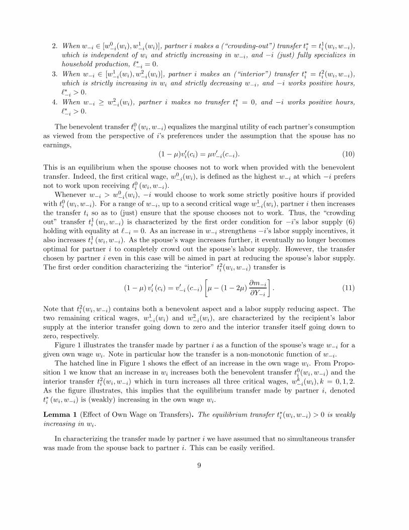
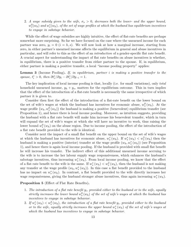
Figure 1 illustrates the transfer made by partner i as a function of the spouse’s wage w−i for agiven own wage wi. Note in particular how the transfer is a non-monotonic function of w−i.

The hatched line in Figure 1 shows the effect of an increase in the own wage wi. From Propo-sition 1 we know that an increase in wi increases both the benevolent transfer t0i (wi, w−i) and theinterior transfer t2i (wi, w−i) which in turn increases all three critical wages, wk

−i(wi), k = 0, 1, 2.As the figure illustrates, this implies that the equilibrium transfer made by partner i, denotedt∗i (wi, w−i) is (weakly) increasing in the own wage wi.

Lemma 1 (Effect of Own Wage on Transfers). The equilibrium transfer t∗i (wi, w−i) > 0 is weaklyincreasing in wi.

In characterizing the transfer made by partner i we have assumed that no simultaneous transferwas made from the spouse back to partner i. This can be easily verified.

9

w−i

ti

w0−i(wi) w1

−i(wi) w2−i(wi)

t0i (wi, w−i)

t1i (wi, w−i)

t2i (wi, w−i)

Figure 1: The transfer made by partner i as a function of the spouse’s wage

Lemma 2 (No Simultaneous Transfers). If partner i makes a positive equilibrium transfer, t∗i (wi, w−i) >0, then the spouse −i strictly prefers not to make a transfer, t∗

−i (w−i, wi) = 0.

Indeed, the proof of Lemma 2 demonstrates that, for any given wi there will exist a rangeof spousal wages w−i such that both i and −i choose not to make any transfer in equilibrium.Hence in a population of couples with a distribution of wage-profile types, equilibrium transferswill be zero for a positive measure of couples. In the limiting case of complete caring (µ = 1/2)the measure of couples who make no transfers reduces to zero as, in the limit, the partners agreeon the consumption allocation and this allocation will, generically, not coincide with the partners’income profile.

To summarize, if one partner makes an equilibrium transfer to the spouse, he/she does soto support the spouse’s private consumption and to influence the spouse’s time allocation awayfrom market work. We now ask whether and when the husband has an incentive to resort to anadditional means of influence, namely economic abuse.

2.4. Incentives for Intrahousehold Sabotage

We identify incentives for economic abuse with the husband’s equilibrium utility being locallydecreasing in the wife’s earnings capacity. The following result, which is interpreted after itsstatement, reveals that the risk of intrahousehold sabotage is present when the economic roleswithin the partnership, in a sense, “hang in the balance”.

Proposition 2 (Economic Incentives for Sabotage). For a given wh (and given yh = ys = 0)there exists a critical wage w∗

s (wh) such that the husband has an incentive to engage in sabotagebehavior when ws ∈ (w0

s(wh), w∗

s(wh)). The critical wage w∗

s (wh) strictly exceeds w1s (wh) and is

weakly increasing in wh.

10

The proposition states that the husband’s incentives for economic abuse kick in when hisbenevolent transfer is not sufficient to induce the wife to fully specialize in household production,i.e. when ws > w0

s(wh), and they continue up to some level of the wife’s wage at which she isworking in equilibrium. The result has a simple intuition. For any ws ≤ w0

s(wh), the husbandmakes the “benevolent transfer” t∗h = t0h(wh, ws), which is sufficient to induce the wife to fullyspecialize in household production. Her wage is low enough to be, in effect, irrelevant and anyfurther reduction in ws would leave the equilibrium entirely unchanged. Thus, the relationship willremain abuse free.

Consider then the case where ws ∈ (w0s(wh), w

1s(wh)), implying that the husband chooses the

crowding out transfer t∗h = t1h(wh, ws). In this case, the husband is making a transfer which exceedsthe one he would voluntarily make, but the wife is still not working in equilibrium. The husband’sequilibrium utility would be increased by a reduction in the wife’s wage as this would allow him toreduce his transfer towards his benevolent transfer. Thus, he has an economic incentive to sabotageher earnings potential.

Finally, consider the case where ws > w1s(wh) so that, in equilibrium, the wife works and the

husband either makes the “interior” transfer t2h(wh, ws) or no transfer at all. In this case, the impactof a marginal increase in the wife’s wage on the husband’s equilibrium utility can be written as

v′s(c∗

s)`∗

s [µ− (1− 2µ) εs (ws, t∗

h)] , (12)

and it can be demonstrated that this expression is strictly negative as ws approaches w1s (wh) from

above (see proof of Proposition 2). This establishes that incentives for economic abuse will also bepresent for some couples where the wife works. The expression in (12) is negative if and only if

µ <εs (ws, t

∗

h)[1 + 2εs

(ws, t∗h

)] . (13)

As the wife’s wage increases, her labour supply responsiveness decreases, thus decreasing the righthand side.9 Instead, for a high enough wife’s wage, his equilibrium utility will be increasing in herwage as he benefits, through caring, from her higher earnings.

Note that in characterizing the husband’s incentives for economic abuse, we have ignored anypotential transfer from the wife to the husband. However, it should be clear enough that anytransfers from the wife to the husband will weaken the husband’s abuse incentives as we knowfrom Lemma 1 that the transfer that the wife makes to the husband will be increasing in her wage.Hence by interfering with her earnings capacity, the husband would also reduce the transfer thathe obtains from her.

Finally, note that economic incentives for intrahousehold sabotage obtain from the inefficiencyin public good provision associated with incomplete caring. The following result shows that, whenpartners behave nearly “completely cooperative”, then they will abstain from abuse altogether:

Proposition 3 (Household Mode of Behavior and Intrahousehold Sabotage). In the limit withcomplete caring, µ → 1

2 , the set of wages profiles ws ∈ (w0s(wh), w

∗

s(wh)) at which the husband hasincentives to engage in sabotage behavior reduces to the empty set.

9When the husband is making the interior transfer t2h (wh, ws) this effect is further reinforced by this transferdecreasing in ws.

11

While this result is highly intuitive, it is at same time in stark contrast to the insights providedby bargaining theories of domestic violence. Indeed, our framework implies that, with completecaring, couples pursue a common objective and the household operates at an agreed point on thePareto frontier. In this cooperative-like setup, an act of sabotage which reduces the wife’s earningscapacity would then simply reduce the utility possibility set and would hence never increase thehusband’s equilibrium utility. In bargaining theories, by contrast, acts of violence occur whenthey increase the utility possibility set and consequently become part of a Pareto-improving trade(involving compensating side-payments) between spouses.

3. The Effect of Welfare Policy

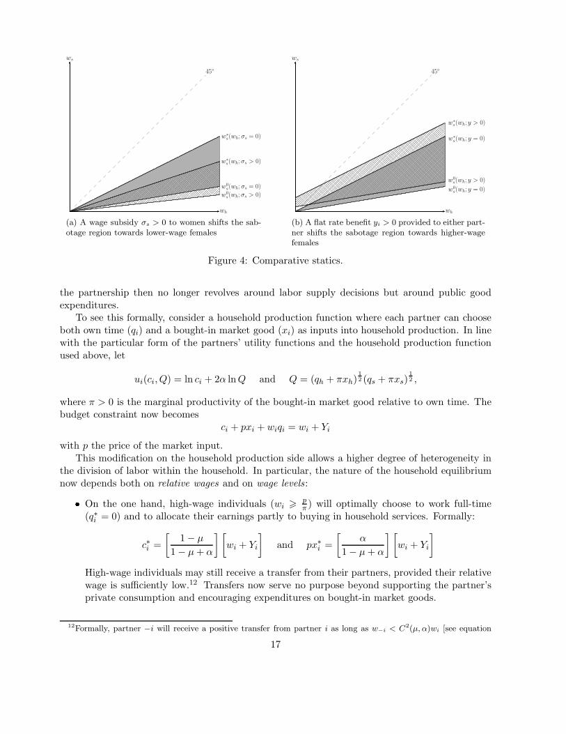
Our analysis provides an instrumental basis for behavior which many others attribute to ataste for sadism or a pleasure of exercising power. This is important because tastes are hard tomanipulate, while incentives are less so. Thus, our theoretical structure allows to get a clear senseof the margins where we may see a change in the incidence of economic abuse when a governmentintervenes with families. In this section, we will consider two very simple examples of policyinterventions: a wage subsidy policy and a flat-rate benefit policy, with either policy potentiallybeing gender-specific.

Consider first a wage subsidy policy and let σi ≥ 0 denote the subsidy rate that applies topartner i, i = h, s. The effective wage for partner i is hence w̃i ≡ (1 + σi)wi, and we refer to wi asthe individual’s primary wage. We are interested in understanding how a wage subsidy offered toeither gender affects the range of wife’s primary wages at which the husband engages in abusivebehavior.

The analysis of wage subsidies is much simplified by the insight that what matters for abuseincentives are the partners’ effective wages. This immediately implies that a wage subsidy providedto women will shift downwards the set of wives’ primary wages at which the husband has incentivesfor sabotage. For example, a woman whose primary wage is low enough that she, in the absence ofa wage subsidy, would choose not to work at the husband’s benevolent transfer may find that, onceprovided with a wage subsidy, she would prefer to work given the same transfer. Hence a wagesubsidy provided to women may expose some low wage women to the risk of abuse. Conversely,a woman whose primary wage would not be high enough to put her beyond the risk of economicabuse, may find that a positive wage subsidy increases her effective wage enough to do so.

Similarly, since the boundaries of the abuse region, w0s (wh) and w∗

s (wh), are increasing in thehusband’s wage, it follows that a wage subsidy provided to the husband shifts upwards the set ofwives’ primary wages at which the husband has incentives for sabotage. Hence, a wage subsidyprovided to the husband will reduce economic abuse against some low wage women who, with thehusband’s subsidy, will choose not to work at his benevolent transfer. Conversely, by reducingthe women’s relative wage, a wage subsidy provided to males, will put into the abuse region somewomen whose wages would otherwise have been sufficiently large to put them beyond the risk ofeconomic abuse.

Proposition 4 (Effect of Wage Subsidies).

1. A wage subsidy given to the husband, σh > 0, increases both the lower- and the upper bound,w0s(wh) and w∗

s(wh), of the set of wage profiles at which the husband has equilibrium incentivesto engage in sabotage behavior.

12

2. A wage subsidy given to the wife, σs > 0, decreases both the lower- and the upper bound,w0s(wh) and w∗

s(wh), of the set of wage profiles at which the husband has equilibrium incentivesto engage in sabotage behavior.

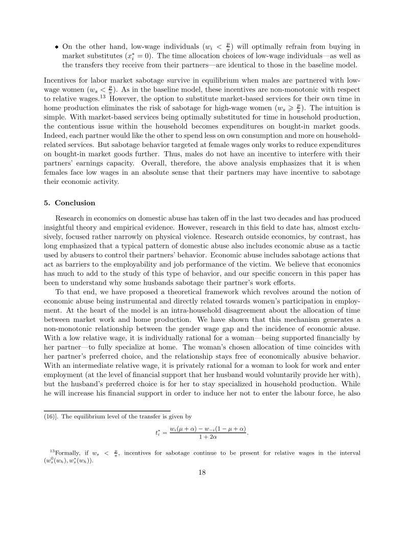
While the effect of wage subsidies are highly intuitive, the effect of flat-rate benefits are perhapssomewhat more surprising. So far we have focused on the case where the unearned income for eachpartner was zero, yi = 0 (i = h, s). We will now look at how a marginal increase, starting fromzero, in either partner’s unearned income affects the equilibrium in general and abuse incentives inparticular, and will refer to this as the effect of an introduction of a gender-specific flat rate benefit.A crucial aspect for understanding the impact of flat rate benefits on abuse incentives is whether,in equilibrium, there is a positive transfer from either partner to the spouse. If, in equilibrium,either partner is making a positive transfer, a local “income pooling property” applies:

Lemma 3 (Income Pooling). If, in equilibrium, partner i is making a positive transfer to thespouse, t∗i > 0, then ∂t∗i /∂yi − ∂t∗i /∂y−i = 1.

The key implication of local income pooling is that, locally (i.e. for small variations), only totalhousehold unearned income, yh + ys, matters for the equilibrium outcome. This in turn impliesthat the effect of the introduction of a flat-rate benefit is necessarily the same irrespective of whichpartner it is given to.

Consider then first the effect of the introduction of a flat-rate benefit on the lower bound onthe set of wife’s wages at which the husband has incentives for economic abuse, w0

s (wh). At thewage profile

(wh, w

0s (wh)

)the husband is making a positive (benevolent) equilibrium transfer (see

Proposition 1), and hence there is local income pooling. Moreover, as intuition suggests, providingthe husband with a flat rate benefit will make him increase his benevolent transfer, which in turnwill expand the set of wife’s wages at which she will have no incentive to work, thus raising thelower bound w0

s (wh) on the abuse region. Due to income pooling, the effect of the introduction ofa flat rate benefit provided to the wife is identical.

Consider next the impact of a small flat benefit on the upper bound on the set of wife’s wagesat which the husband has incentives for economic abuse, w∗

s (wh). If w∗

s (wh) < w2s (wh) then the

husband is making a positive (interior) transfer at the wage profile (wh, w∗

s (wh)) (see Proposition1), and hence there is again local income pooling. If the husband is provided with small flat benefithe will increase his transfer. The indirect effect of this additional unearned income accruing tothe wife is to increase the her labour supply wage responsiveness, which enhances the husband’ssabotage incentives, thus increasing w∗

s (wh). From local income pooling, we know that the effectof a flat rate benefit to the wife is the same. If w∗

s (wh) < w2s (wh), then the husband is not making

any transfer at the wage profile (wh, w∗

s (wh)). In this case a flat benefit provided to the husbandhas no impact on w∗

s (wh). In contrast, a flat benefit provided to the wife directly increases herwage responsiveness, giving the husband stronger abuse incentives, thus again increasing w∗

s (wh).

Proposition 5 (Effect of Flat Rate Benefits).

1. The introduction of a flat rate benefit yi, provided either to the husband or to the wife, equallystrictly increases the lower bound w0

s (wh) of the set of wife’s wages at which the husband hasincentives to engage in sabotage behavior.

2. If w∗

s (wh) < w2s (wh), the introduction of a flat rate benefit yi, provided either to the husband

or to the wife, equally strictly increases the upper bound w∗

s (wh) of the set of wife’s wages atwhich the husband has incentives to engage in sabotage behavior.

13

3. If w∗

s (wh) > w2s (wh), the introduction of a flat rate benefit ys provided to the wife strictly

increases w∗

s (wh) whereas a corresponding flat rate benefit yh provided to the husband has noeffect on w∗

s (wh).

Our results, so far, suggest that welfare policies may shift the incidence of economic abusewithout necessarily reducing it: wage subsidies to women shift the incidence of economic abusedownwards in the female wage distribution. Conversely, unconditional family cash benefits shiftshift the incidence of economic abuse upwards in the female wage distribution. Each policy inisolation may, therefore, have undesirable effects on the risk of domestic abuse for some women.These observations permit us to deduce what type of policy mix would, according to the model,reduce the incidence of economic abuse. Such a policy mix would require: (1) cash benefits tocouples in the low-wage and low-to-medium wage regime, which would allow males to prevent theinefficiency of non-cooperative equilibrium by means of a benevolent transfer instead of sabotage;and (2) wage subsidies to women in the medium-to-high wage regime, which would reinforce theimportance of female earnings for the household, and so induce males to abstain from sabotagebehavior.

4. A Cobb-Douglas Example

In this section we provide a simple Cobb-Douglas example which, in addition to illustratingthe model, allows us to highlight a few more of its features. Hence we let

ui(ci, Q) = ln ci + 2α lnQ and Q (qh, qs) = q1/2h q1/2s . (14)

In this specification we include the parameter α > 0 as a measure of the relative importance of thehousehold produced good.

A feature of the Cobb-Douglas specification (with zero exogenous unearned incomes) is thatthe nature of the household equilibrium depends only on the relative wages ws/wh, not on wagelevels. In particular, maintaining the assumption that yh = ys = 0, the critical wages partitioningthe transfer regimes can all be written in the form

wk−i (wi) = Ck (µ, α)wi, (15)

with

C0 (µ, α) =αµ

(α+ 1) (1− µ)

C1 (µ, α) =α (α+ µ)

3α (1− µ)− µ+ α2 + 1

C2 (µ, α) =(α+ µ)

(1 + α− µ).

(16)

In a similar way, the upper boundary on the set of wife’s wages at which the husband has incentivesfor economic abuse can be written in the form

w∗

s (wh) = C∗ (α)wh with C∗ (α) =α

α+ 1. (17)

14

wh

ws

45◦

w0s(wh)

w1s(wh)

w2s(wh)

w0h(ws) w1

h(ws) w2h(ws)

t0h

t1h

t2h

t0s t1s t2s th = ts = 0

(a) Regions by transfer regime and labor sup-ply

wh

ws

45◦

w0s(wh)

w1s(wh)

w2s(wh)

w∗s(wh)

w0h(ws) w1

h(ws) w2h(ws)

t0h

t1h

t2h

t0s t1s t2s th = ts = 0

(b) Region with incentives for intrahouseholdsabotage

Figure 2: Illustration of the equilibrium.

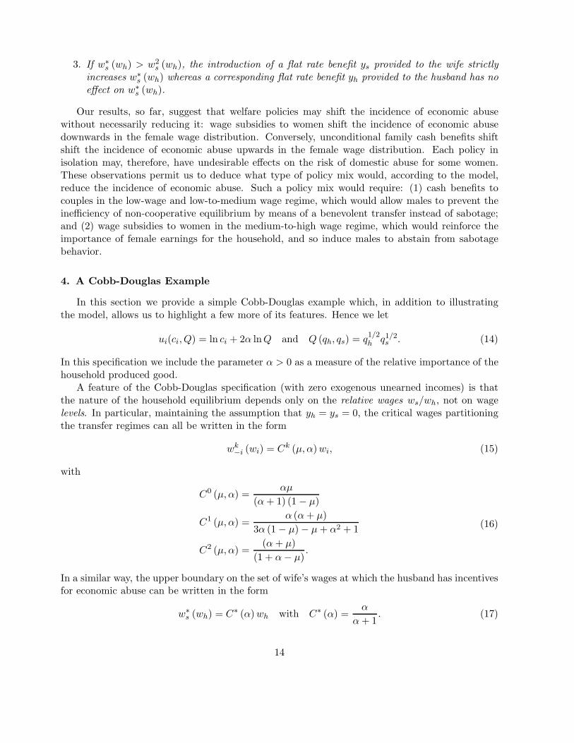
As (17) indicates, in the Cobb-Douglas example, the upper bound on the set of wife’s relativewages at which the husband has incentives for economic abuse wage does not actually depend onµ but depends positively on α. Note that C2 (µ, α) > C∗ (α). Hence in the Cobb-Douglas case,economic abuse always coexist with positive transfers from the husband to the wife. This resultfollows from the fact that, with Cobb-Douglas preferences and with ys = 0, the wife’s labour supplyresponsiveness, εs (ws, th), drops to zero when she does not receive a transfer from the husband.Hence the husband cannot influence the wife’s labour supply by saboting her wage unless he alsomakes a positive transfer.

Figure 2(a) illustrates how the space of wage-profiles is partitioned into regions with differentnature/direction of transfers and labour supply status for the case of µ = 1/4 and α = 1. Atws < w0

s (wh) the husband makes the “benevolent” transfer t0h (wh, ws) and the wife strictly prefersnot to work. At ws ∈

(w0s (wh) , w

1s (wh)

)the husband makes the “crowding out” transfer t1h (wh, ws)

and the wife just chooses not to work. At ws ∈(w1s (wh) , w

2s (wh)

)the husband makes an “interior”

transfer t2h (wh, ws) and the wife works positive hours. At higher wife’s wages, the husband doesmake any transfer to the wife. As, in this example, preferences are symmetric across the twogenders, corresponding regions apply when the wife’s wage exceeds the husbands.

Figure 2(b) illustrates in the same example the set of wage profiles at which the husband hasincentives to engage in sabotage behavior. The figure illustrates how incentives for sabotage obtainfor a set of wage profiles around those where the wife enters the labour market.

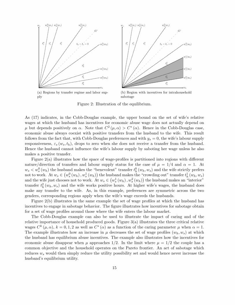
The Cobb-Douglas example can also be used to illustrate the impact of caring and of therelative importance of household produced goods. Figure 3(a) illustrates the three critical relativewages Ck (µ, α), k = 0, 1, 2 as well as C∗ (α) as a function of the caring parameter µ when α = 1.The example illustrates how an increase in µ decreases the set of wage profiles (wh, ws) at whichthe husband has equilibrium abuse incentives. The example also illustrates how the incentives foreconomic abuse disappear when µ approaches 1/2. In the limit where µ = 1/2 the couple has acommon objective and the household operates on the Pareto frontier. An act of sabotage whichreduces ws would then simply reduce the utility possibility set and would hence never increase thehusband’s equilibrium utility.

15

0

0.1

0.2

0.3

0.4

0.5

0.6

0.7

0.8

0.9

1.0

0 0.1 0.2 0.3 0.4 0.5µ

ws/wh

C0(µ, α = 1)

C1(µ, α = 1)

C2(µ, α = 1)

C∗(α = 1)

(a) Transfer and sabotage regions as a function ofcaring

0

0.1

0.2

0.3

0.4

0.5

0.6

0.7

0.8

0.9

0 0.2 0.4 0.6 0.8 1.0 1.2 1.4 1.6 1.8 2.0α

ws/wh

C0(µ = 1/4, α)

C1(µ = 1/4, α)

C2(µ = 1/4, α)

C∗(α)

(b) Transfer and sabotage regions as a functionof the importance of household production

Figure 3: Comparative statics.

Figure 3(b) illustrates the same critical relative wage functions, now as a function of α givenµ = 1/4. This figure highlights how an increase in the relative importance of household production,as parameterized by α, tends to increase the incentives for economic abuse. This reflects how, inthe current model, economically abusive behavior obtains as a result of disagreements betweenthe two partners regarding the allocation of time in the presence of household production: if theimportance of household produced goods diminish, so do the incentives for sabotage.

Above we outlined some general results regarding the effect of wage subsidies and flat-ratebenefits on the incidence of economic abuse. In line with the result that only relative wages matterin the Cobb-Douglas, it is only the relative subsidy rate that matters for abuse incentives.10

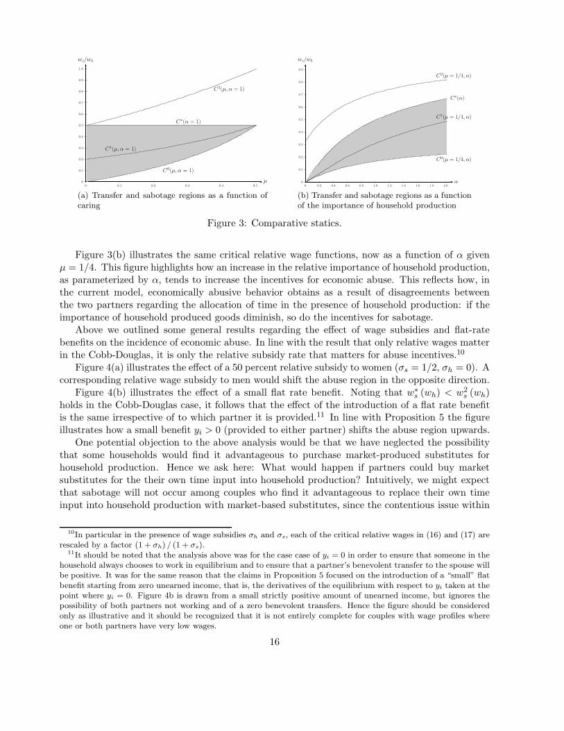
Figure 4(a) illustrates the effect of a 50 percent relative subsidy to women (σs = 1/2, σh = 0). Acorresponding relative wage subsidy to men would shift the abuse region in the opposite direction.

Figure 4(b) illustrates the effect of a small flat rate benefit. Noting that w∗

s (wh) < w2s (wh)

holds in the Cobb-Douglas case, it follows that the effect of the introduction of a flat rate benefitis the same irrespective of to which partner it is provided.11 In line with Proposition 5 the figureillustrates how a small benefit yi > 0 (provided to either partner) shifts the abuse region upwards.

One potential objection to the above analysis would be that we have neglected the possibilitythat some households would find it advantageous to purchase market-produced substitutes forhousehold production. Hence we ask here: What would happen if partners could buy marketsubstitutes for the their own time input into household production? Intuitively, we might expectthat sabotage will not occur among couples who find it advantageous to replace their own timeinput into household production with market-based substitutes, since the contentious issue within

10In particular in the presence of wage subsidies σh and σs, each of the critical relative wages in (16) and (17) arerescaled by a factor (1 + σh) / (1 + σs).

11It should be noted that the analysis above was for the case case of yi = 0 in order to ensure that someone in thehousehold always chooses to work in equilibrium and to ensure that a partner’s benevolent transfer to the spouse willbe positive. It was for the same reason that the claims in Proposition 5 focused on the introduction of a “small” flatbenefit starting from zero unearned income, that is, the derivatives of the equilibrium with respect to yi taken at thepoint where yi = 0. Figure 4b is drawn from a small strictly positive amount of unearned income, but ignores thepossibility of both partners not working and of a zero benevolent transfers. Hence the figure should be consideredonly as illustrative and it should be recognized that it is not entirely complete for couples with wage profiles whereone or both partners have very low wages.

16

wh

ws

45◦

w0s(wh; σs = 0)

w0s(wh;σs > 0)

w∗s(wh; σs = 0)

w∗s(wh; σs > 0)

(a) A wage subsidy σs > 0 to women shifts the sab-otage region towards lower-wage females

wh

ws

45◦

w0s(wh; y = 0)

w0s(wh; y > 0)

w∗s(wh; y = 0)

w∗s(wh; y > 0)

(b) A flat rate benefit yi > 0 provided to either part-ner shifts the sabotage region towards higher-wagefemales

Figure 4: Comparative statics.

the partnership then no longer revolves around labor supply decisions but around public goodexpenditures.

To see this formally, consider a household production function where each partner can chooseboth own time (qi) and a bought-in market good (xi) as inputs into household production. In linewith the particular form of the partners’ utility functions and the household production functionused above, let

ui(ci, Q) = ln ci + 2α lnQ and Q = (qh + πxh)1

2 (qs + πxs)1

2 ,

where π > 0 is the marginal productivity of the bought-in market good relative to own time. Thebudget constraint now becomes

ci + pxi + wiqi = wi + Yi

with p the price of the market input.This modification on the household production side allows a higher degree of heterogeneity in

the division of labor within the household. In particular, the nature of the household equilibriumnow depends both on relative wages and on wage levels:� On the one hand, high-wage individuals (wi >

pπ ) will optimally choose to work full-time

(q∗i = 0) and to allocate their earnings partly to buying in household services. Formally:

c∗i =

[1− µ

1− µ+ α

] [wi + Yi

]and px∗i =

[α

1− µ+ α

] [wi + Yi

]

High-wage individuals may still receive a transfer from their partners, provided their relativewage is sufficiently low.12 Transfers now serve no purpose beyond supporting the partner’sprivate consumption and encouraging expenditures on bought-in market goods.

12Formally, partner −i will receive a positive transfer from partner i as long as w−i < C2(µ, α)wi [see equation

17

� On the other hand, low-wage individuals (wi < pπ ) will optimally refrain from buying in

market substitutes (x∗i = 0). The time allocation choices of low-wage individuals—as well asthe transfers they receive from their partners—are identical to those in the baseline model.

Incentives for labor market sabotage survive in equilibrium when males are partnered with low-wage women (ws <

pπ ). As in the baseline model, these incentives are non-monotonic with respect

to relative wages.13 However, the option to substitute market-based services for their own time inhome production eliminates the risk of sabotage for high-wage women (ws >

pπ ). The intuition is

simple. With market-based services being optimally substituted for time in household production,the contentious issue within the household becomes expenditures on bought-in market goods.Indeed, each partner would like the other to spend less on own consumption and more on household-related services. But sabotage behavior targeted at female wages only works to reduce expenditureson bought-in market goods further. Thus, males do not have an incentive to interfere with theirpartners’ earnings capacity. Overall, therefore, the above analysis emphasizes that it is whenfemales face low wages in an absolute sense that their partners may have incentive to sabotagetheir economic activity.

5. Conclusion

Research in economics on domestic abuse has taken off in the last two decades and has producedinsightful theory and empirical evidence. However, research in this field to date has, almost exclu-sively, focused rather narrowly on physical violence. Research outside economics, by contrast, haslong emphasized that a typical pattern of domestic abuse also includes economic abuse as a tacticused by abusers to control their partners’ behavior. Economic abuse includes sabotage actions thatact as barriers to the employability and job performance of the victim. We believe that economicshas much to add to the study of this type of behavior, and our specific concern in this paper hasbeen to understand why some husbands sabotage their partner’s work efforts.

To that end, we have proposed a theoretical framework which revolves around the notion ofeconomic abuse being instrumental and directly related towards women’s participation in employ-ment. At the heart of the model is an intra-household disagreement about the allocation of timebetween market work and home production. We have shown that this mechanism generates anon-monotonic relationship between the gender wage gap and the incidence of economic abuse.With a low relative wage, it is individually rational for a woman—being supported financially byher partner—to fully specialize at home. The woman’s chosen allocation of time coincides withher partner’s preferred choice, and the relationship stays free of economically abusive behavior.With an intermediate relative wage, it is privately rational for a woman to look for work and enteremployment (at the level of financial support that her husband would voluntarily provide her with),but the husband’s preferred choice is for her to stay specialized in household production. Whilehe will increase his financial support in order to induce her not to enter the labour force, he also

(16)]. The equilibrium level of the transfer is given by

t∗i =wi(µ+ α)− w−i(1− µ+ α)

1 + 2α.

13Formally, if ws < p

π, incentives for sabotage continue to be present for relative wages in the interval

(w0

s(wh), w∗

s(wh)).

18

has an incentive to directly interfere with her labour market opportunities and hence resorts tosabotage tactics. Finally, with a high relative wage, a woman’s earned income is too important fora male partner to interfere with her earnings capacity. Overall, therefore, our model predicts thateconomic abuse in the form of labor market sabotage is associated with a woman’s labor supplybeing contentious and economic roles in the family hanging in the balance.

In addition to suggesting an interpretation for the economic abuse component of domesticviolence, our analysis also serves to highlight some policy dilemmas. Our results suggest thatpolicies aimed at improving the economic situation of families may shift the incidence of economicabuse without necessarily reducing it. For example, unconditional family cash benefits shift theincidence of economic abuse upwards in the female wage distribution, while wages subsidies towomen may have the opposite effect. In order to reduce the risk of economic abuse, therefore,different types of households have to be targeted with different types of policy measures. Thisunderlines the complexities policy makers have to negotiate when facing the problem of economicabuse, which many analysts consider to be just as harmful as other forms of domestic abuse.

It is important to acknowledge that this paper is a purely theoretical exercise. In general,we know precious little about the empirical importance of the channels identified by our theory.Most of the empirical literature has taken as its null hypothesis that the risk of domestic violencemonotonically decreases with women’s relative wages. This paper establishes an alternative hy-pothesis based on the idea that men may have an incentive to impose negative outcomes on theirpartners when spousal preferences regarding the intrahousehold allocation of time are misaligned.This alternative hypothesis explains existing evidence on economically abusive behavior and givesdirection for future empirical research.

There are several directions in which our analysis could be expanded. From a theoreticalperspective, it would be interesting to embed the present framework in a model where womenhave the option of quitting abusive relationships and use the unifying model to examine howthe internal organization of the family and outside options interact in shaping the incidence ofdomestic abuse. From an empirical perspective, it would be interesting to use survey data todeduce some of the key parameters of our model and to generate quantitative predictions from theestimated parameter values. This would allow us to get a feel for the empirical relevance of thenon-monotonic relationship between the gender wage gap and the incidence of abuse as predictedby the theory. These and other issues are important and challenging topics for future research. Inthe meantime, our analysis demonstrates the value of going beyond preference-based bargainingmodels of domestic violence and to incorporate instrumental incentives into economic explanationsof spousal abuse against women.

References

Adams, A., Sullivan, C., Bybee, D. and Greeson, M. (2008). Development of the scale of economic abuse.Violence Against Women, 14 (5), 563–588.

Aizer, A. (2010). The gender wage gap and domestic violence. American Economic Review, 100, 1847–1859.Anderberg, D. (2007). Inefficient households and the mix of government spending. Public Choice, 131, 127–140.Bazelon, E. (2009). The sabotaging husband. Forbes, available at http://www.forbes.com/2008/10/13/0929 FLEW087.html.Becker, G. S. (1991). A Treatise on the Family. Harvard Universtiy Press.Bergstrom, T. (1989). A fresh look at the rotten kid theorem. Journal of Political Economy, 97, 1138–1159.Bloch, F. and Rao, V. (2002). Terror as a bargaining instrument: A case study of dowry violence in rural India.

American Economic Review, 92.Brandwein, R. and Filiano, D. (2000). Toward realwelfare reform: The voices of battered women. Affilia, 15 (2),

224–243.

19

Card, D. and Dahl, G. (2011). Family violence and football: The effect of unexpected emotional cues on violentbehavior. Quarterly Journal of Economics, forthcoming.

Chen, Z. and Woolley, F. (2001). A cournot-nash model of family decision making. Economic Journal, 111,722–748.

Chiappori, P. A. (1992). Collective labor supply and welfare. Journal of Political Economy, 100, 437–462.—, Fortin, B. and Lacroix, G. (202). Marriage market, divorce legislation, and household labor supply. Journal

of Political Economy, 110, 37–72.Del Boca, D. and Flinn, C. (2012). Endogeneous household interaction. Journal of Econometrics, 166 (1), 49–65.Farmer, A. and Tiefenthaler, J. (1997). An economic analysis of domestic violence. Review of Social Economy,

55, 337–358.Johnson, H. (1995). The truth about white-collar domestic violence. Working Woman, 20, 54–57.Kondrad, K. A. and Lommerud, K. E. (1995). Family policy with non-cooperative families. Scandinavian Journal

of Economics, 97, 581–601.Lundberg, S. and Pollak, R. (1993). Separate spheres bargaining and the marriage market. Journal of Political

Economy, 101, 988–1010.Manser, M. and Brown, M. (1980). Marriage and household decision-making: A bargaining analysis. International

Economic Review, 21 (1), 31–44.McElroy, M. and Horney, M. (1981). Nash-bargained household decisions: Toward a generalization of the theory

of demand. International Economic Review, 22 (2), 333–349.Pearson, J., Theonnes, N. and Griswold, E. A. (1999). Child support and domestic violence: The victims speak

out. Violence Against Women, 5, 427–448.Raphael, J. (1995). Domestic violence: Telling the untold welfare-to-work story. Taylor Institute, 915 N. Wolcott,

Chicago, IL 60222.— (1996). Prisoners of abuse: Domestic violence and welfare receipt. Taylor Institute, 915 N. Wolcott, Chicago, IL

60222.Riger, S., Ahrens, C. and Blickenstaff, A. (2000). Measuring interference with employment and education

reported by women with abusive partners: Preliminary data. Violence and Victims, 15, 161–172.Swanberg, J. and Logan, T. (2004). Intimate partner violence, women and work: Findings from the first wave of

a longitudinal study. Unpublished Manuscript, University of Kentucky.— and Macke, C. (2006). Intimate partner violence and the workplace: Consequences and disclosures. Journal of

Women and Social Work, 21 (4), 391–406.Tauchen, H. V., Witte, A. D. and Long, S. K. (1991). Violence in the family: A non-random affair. International

Economic Review, 32, 491–511.Tjaden, P. and Thoennes, N. (1998). The prevalence, incidence and consequences of violence against women:

Findings from the national violence against women survey. Washington DC: US Department of Justice, OJP.Report No: NCJ 172837.

Tolman, R. and Rosen, D. (2001). Domestic violence in the lives of women receiving welfare: Mental health, health,and economic well-being. Violence Against Women, 7, 141–158.

Tolman, R. M. and Raphael, J. (2000). A review of research on welfare and domestic violence. Journal of SocialIssues, 56, 655–682.

Zachary, M. (2000). Labor law for supervisors: Domestic violence as a workplace issue. Supervision, 61 (4), 23–26.

20

Appendix

Proof of Proposition 1. It should be noted that the proposition is derived under the assumption of zerounearned income for each partner. Hence while we retain the general notation for unearned incomes, yi andy−i, all equations etc. in the proof of the current proposition should are evaluated at yi = y−i = 0.

The proposition is proven through a series of lemmas. First, define the “benevolent” transfer, t0i (wi, w−i),from partner i to −i implicitly as the solution to the following equation:

(1− µ) v′i(mi

(wi, yi − t0i (wi, w−i)

)+ yi − t0i (wi, w−i)

)= µv′−i

(y−i + t0i (wi, w−i)

). (A1)

Lemma A.1. The benevolent transfer t0i (wi, w−i) is (i) a uniquely identified continuous function witht0i (wi, w−i) ∈ (0, wi), (ii) strictly increasing in wi and independent of w−i.

Proof. Both sides of (A1) are continuous functions of ti. Using (9) it follows that the left hand side isstrictly increasing in ti. The right hand side is strictly decreasing in ti. Moreover, as ti approaches either 0the right hand side approaches infinity whereas if ti approaches wi, the left hand side approaches infinity.Hence (A1) must have a unique solution in the interval (0, wi). The effect of an increase in wi follows fromthe fact that ∂mi/∂wi > 0. Independence of w−i follows from the fact that it does not feature directly in(A1).

Next, define the “crowding out” transfer, t1i (wi, w−i), from partner i to −i implicitly as the transfer atwhich −i just chooses zero labour supply:

v′−i

(y−i + t1i (wi, w−i)

)=

1

w−i

z′−i (1)

(1− µ). (A2)

Lemma A.2. The crowding out transfer t1i (wi, w−i) is (i) a uniquely identified continuous function, (ii)strictly increasing in w−i, independent of wi,(iii) approaches 0 as w−i approaches 0.

Proof. Uniqueness and continuity follow immediately from differentiability and strict concavity of v−i (·).Monotonicity in w−i follows from strict concavity of v−i (·). Independence of wi follows from the fact thatwi does not feature directly in (A2). Finally, note that as w−i → 0+, any positive transfer will strictlyinduce −i not to work. Hence t1i (wi, w−i) (which is the smallest transfer at which −i chooses not to work)must approach zero.

For large enough w−i, the crowding out transfer will not be “affordable” to i. Hence we implicitly definewmax

−i (wi) as the w−i at which the crowding out transfer corresponds to i’s maximum earnings.

t1i(wi, w

max−i (wi)

)= wi. (A3)

From the properties of t1i (wi, w−i) in Lemma A.2 it follows that wmax−i (wi) is uniquely identified and strictly

increasing in wi.We next define w0

−i(wi) as w−i which equates the benevolent and the crowding out transfer,

t0i(wi, w

0−i(wi)

)= t1i

(wi, w

0−i(wi)

). (A4)

Lemma A.3. The critical wage w0−i (wi) is a uniquely identified continuous and strictly increasing function

of wi, and w−i < (>)w0−i (wi) implies t0i (wi, w−i) > (<) t1i (wi, w−i).

Proof. Immediate from the properties of t0i (wi, w−i) and t1i (wi, w−i) given in Lemma A.1 and A.2.

21

In order to analyze the transfer decision it is useful to write −i’s utility as a (continuous) function of tiin the following way

Ui (ti;wi, w−i) ≡ (1− µ) vi (mi (wi, yi − ti) + yi − ti) + µv−i (m−i (w−i, y−i + ti) + y−i + ti)

+z

(1−

mi (wi, yi − ti)

wi

, 1−m−i (w−i, y−i + ti)

w−i

), (A5)

remembering that for any ti ≥ t1i (wi, w−i) the recipient, −i, chooses zero labor supply. We can now establishstrict concavity of −i’s utility in ti.

Lemma A.4. Ui (ti;wi, w−i) is strictly a strictly concave function of ti with a “downward kink” at ti =t1i (wi, w−i).

Proof. Differentiating (A5) with respect to ti and evaluating at some ti < t1i (wi, w−i) yields, after substi-tuting using (6),

∂Ui (ti;wi, w−i)

∂ti= − (1− µ) v′i (ci) + v′−i (c−i)

[µ− (1− 2µ)

∂m−i

∂Y−i

]. (A6)

When evaluating at some ti > t1i (wi, w−i), the same expression holds but with ∂m−i/∂Y−i = 0 as −i strictlyprefers not to work at such a transfer. At ti = t1i (wi, w−i), the derivative (A6) does not exist. However,the left and the right derivatives both exist and are given by (A6), with and without the ∂m−i/∂Y−i termincluded respectively. Since ∂m−i/∂Y−i < 0 (see eq. (9)), the left derivative exceeds the right derivative.

Differentiating a second time and evaluating at some ti < t1i (wi, w−i) yields

∂2Ui (ti;wi, w−i)

∂t2i= (1− µ) v′′i (ci)

(1 +

∂mi

∂Yi

)+ v′′−i (c−i)

(1 +

∂m−i

∂Y−i

)[µ− (1− 2µ)

∂m−i

∂Y−i

]

−v′−i (c−i) (1− 2µ)∂2m−i

∂Y 2−i

. (A7)

When evaluating at some ti > t1i (wi, w−i), the same expression holds but with ∂m−i/∂Y−i = 0 etc. Itfollows from (9) and Assumption 3, that (A7) is strictly negative at any ti 6= t1i (wi, w−i).

From Lemma A.4 it follows that i’s optimal transfer (if positive) is either characterized by ti 6=t1i (wi, w−i) and (A6) being equal to zero, or by ti = t1i (wi, w−i) and (A6) being strictly positive at allti < t1i (wi, w−i) and strictly negative at all ti > t1i (wi, w−i)). For future reference it is also useful to notethat, when evaluated at some ti < t1i (wi, w−i),

∂2Ui (ti;wi, w−i)

∂ti∂w−i

= v′′−i (c−i)∂m−i

∂w−i

[µ− (1− 2µ)

∂m−i

∂Y−i

]− v′−i (c−i) (1− 2µ)

∂2m−i

∂Y−i∂w−i

< 0, (A8)

where the inequality follows from Assumption 3. When evaluated at some ti > t1i (wi, w−i) the expressionin (A8) is identically equal to zero as −i then strictly prefer to not work. Note also that

∂2Ui (ti;wi, w−i)

∂ti∂wi

= − (1− µ) v′′i (ci)∂mi

∂wi

> 0. (A9)

Lemma A.5. At w−i ≤ w0−i (wi), i’s optimal transfer is the benevolent transfer t0i (wi, w−i).

Proof. Suppose that w−i ≤ w0−i (wi) and i chooses ti = t0i (wi, w−i). Since t0i (wi, w−i) ≥ t1i (wi, w−i) (see

Lemma A.3), it follows from the definition of the benevolent transfer in (A1) that ∂Ui/∂ti given by (A6)equals zero at this transfer, thus confirming that it is an optimal choice for i.

22

Next we define implicitly a second critical recipient’s wage. To this end, consider the left derivative of(A5) with respect to ti, evaluated at the limit point ti = t1i (wi, w−i),

∂Ui

(t1i (wi, w−i) ;wi, w−i

)

∂t−i= 0, (A10)

where we note that the left derivative is given by (A6) with the inclusion of the ∂m−i/∂Y−i term. Thesecond critical wage, denoted w1

−i (wi), is implicitly defined as the w−i at which (A10) equals zero.

Lemma A.6. The critical wage w1−i (wi) (i) is a uniquely identified continuous and strictly increasing

function of wi, and (ii) is strictly larger than w0−i (wi).

Proof. Evaluating atw−i ≤ w0−i (wi), and using that, at any such recipient’s wage, t1i (wi, w−i) ≤ t0i (wi, w−i),

one can easily verify that the left hand side of (A10) is positive. For large enough w−i, (A10) will, on theother hand, be negative. To see this, note that when w−i approaches w

max−i (wi), t

1i (wi, w−i) approaches wi,

implying that i’s consumption approaches zero. Given continuity of the left hand side of (A10) in w−i atleast one solution to the equation in (A10) exists, and any solution strictly exceeds w0

−i (wi).To demonstrate uniqueness of w1

−i (wi), note that (A10) is strictly decreasing in w−i both directly (seeeq. A8), and indirectly via t1i (wi, w−i) being increasing in w−i (Lemma A.2) and concavity of Ui in ti(Lemma A.4). Finally, that w1

−i (wi) is increasing in wi follows from simple comparative statics using (A9)and recalling that t1i (wi, w−i) is independent of wi (Lemma A.2)

Lemma A.7. At w−i ∈(w0

−i(wi), w1−i(wi)

), i’s optimal transfer is the crowding-out transfer t1i (wi, w−i).

Proof. For w−i ∈(w0

−i(wi), w1−i(wi)

)we now have that the right derivative of Ui (ti;wi, w−i) with respect

to ti evaluated at ti = t1i (wi, w−i) is strictly negative (since, for such w−i, t1i (wi, w−i) > t0i (wi, w−i)) while

the left derivative is strictly positive. Hence, by global concavity of Ui (ti;wi, w−i) in ti (Lemma A.4) itfollows that t1i (wi, w−i) is i’s optimal transfer.

We define a third critical recipient’s wage, denoted w2−i (wi), as the smallest w−i at which i chooses to

make a zero transfer. Specifically, we define w2−i (wi) implicitly through the following equation,

∂Ui

(0;wi, w

2−i (wi)

)

∂ti= 0. (A11)

Lemma A.8. The critical wage w2−i (wi) (i) is a uniquely identified continuous and strictly increasing

function of wi, and (ii) is strictly larger than w1−i (wi).

Proof. From Lemmas A.5 and A.7, we know that for any w−i ≤ w1−i (wi), i’s optimal transfer is either

t1i (wi, w−i) or, if w−i ≤ w0−i (wi) , t0i (wi, w−i) which then exceeds t1i (wi, w−i). Hence for any w−i ≤

w1−i (wi), i’s optimal transfer is strictly positive, implying that ∂Ui (0;wi, w−i) /∂ti is strictly positive at any

such w−i. Next we note that ∂Ui (0;wi, w−i) /∂ti is strictly decreasing in w−i as −i’s earnings are increasingin w−i and due to Assumption 3 (and, under natural conditions, for large enough w−i the derivative becomesnegative). This demonstrates that w2

−i (wi) is unique and exceeds w1−i (wi). That w2

−i (wi) increases in wi

follows from (A9).

Lemma A.9. At w−i ∈(w1

−i (wi) , w2−i (wi)

), i’s optimal transfer is an “interior” transfer t2i (wi, w−i),

where t2i (wi, w−i) ∈(0, t1i (wi, w−i)

)and is strictly increasing in wi and strictly decreasing in w−i. At

w−i ≥ w2−i (wi), i’s optimal transfer is the zero transfer.

Proof. For w−i > w1−i(wi), the left derivative of Ui (ti;wi, w−i) with respect to ti evaluated at ti =

t1i (wi, w−i) is strictly negative, implying that i’s optimal transfer is given by some ti < t1i (wi, w−i) (atwhich the recipient works some positive amount of time). The optimal transfer in this case is either strictlypositive and characterized by the derivative in (A6) being equal to zero, or equal to zero with the derivative

23

in (A6) being non-positive at ti = 0. Per definition, w2−i (wi) is the unique recipient’s wage above which

the derivative of Ui (ti;wi, w−i) with respect to ti evaluated at ti = 0 is negative. We denote the strictlypositive transfer made at w−i ∈

(w1

−i (wi) , w2−i (wi)

)by t2i (wi, w−i). Monotonicity of t2i (wi, w−i) in wi and

w−i then follows immediately from (A8) and (A9).

Proposition 1 follows in a straightforward manner, using Lemmas A.1 to A.9.

Proof of Lemma 2. Suppose that, in equilibrium, partner i is making a positive transfer to partner −i. Itthen follows that

(1− µ) v′i (ci) ≤ v′−i (c−i)

[µ− (1− 2µ)

∂m−i

∂Y−i

]. (A12)

To see this, note that if i makes an interior transfer t2i (wi, w−i) to −i, then (A12) holds with equality as itis the first order condition characterizing the interior transfer. If i makes a benevolent transfer t0i (wi, w−i)to −i, then (A12) holds with equality, but with ∂m−i/∂Y−i = 0 as −i strictly prefers not to work. Finally,if i is making the crowding out transfer t1i (wi, w−i) to −i, then (A12) holds with inequality as the leftderivative of Ui with respect ti at t

1i (wi, w−i) is positive (see proof of Proposition 1). If partner −i is then

also making a positive transfer to i, the same inequality with i and −i interchanged also holds. Combiningthe two inequalities to eliminate the marginal utilities yields that

(1− µ)2≤

[µ− (1− 2µ)

∂mi

∂Yi

] [µ− (1− 2µ)

∂m−i

∂Y−i

]. (A13)

However, this is a contradiction since the right hand side is, for any µ ∈ [0, 1/2) and(

∂mh

∂Yh

, ∂mh

∂Yh

)∈

(−1, 0)× (−1, 0), in the open interval(µ2, (1− µ)2

).

Proof of Proposition 2. Let U∗i (wi, w−i) denote the equilibrium utility of partner i. At any ws ≤ w0

s (wh),the husband makes the “benevolent transfer” t0h (wh, ws) which is independent of ws, and the wife strictlyprefers not to work in equilibrium. A marginal reduction ws does not affect any aspect of the equilibrium,and hence, in particular, does not increase the husband’s equilibrium utility U∗

h (wh, ws).At any ws ∈

(w0

s (wh) , w1s (wh)

]the husband chooses the “crowding-out transfer” t1h (wh, ws) and, in

equilibrium, the wife just chooses not to work. At such a ws it follows that

∂U∗h (wh, ws)

∂ws

= − [(1− µ) v′h (c∗h)− µv′s (c

∗s)]

∂t1h (wh, ws)

∂ws

< 0, (A14)

where the sign follows from the fact that, as ws > w0s (wh), t

1h (wh, ws) > t0h (wh, ws) (see Lemma A.3),

implying that the term in brackets is positive.At any wage ws ∈

(w1

s (wh) , w2s (wh)

)the husband chooses the “interior transfer” t2h (wh, ws) and, in

equilibrium, the wife is working some positive amount of time in the labour market. At such a ws it can beshown, after simplifying using the first order conditions for labour supplies and the characterization of the“interior” transfer, that

∂U∗h (wh, ws)

∂ws

= µv′s (c∗s)

[ws

∂`∗s∂ws

+ `∗s

]− z′s (q

∗s )

∂`∗s∂ws

(A15)

Substituting for z′s (q∗s ) in the final term using the first order condition for the wife’s labour supply and

collecting terms, this can be rewritten as

∂U∗h (wh, ws)

∂ws

= v′s (c∗s) `

∗s {µ− (1− 2µ) εs (ws, ys + t∗h)} . (A16)

24

It should be noted that the husband’s incentives for abuse are “smooth” at ws = w1s (wh): taking the limit

of (A14) as ws → w1s (wh)

−and the limit of (A16) as ws → w1

s (wh)+, and using simple comparative statics,

yields that

limws↗w1

s(wh)

∂U∗h (wh, ws)

∂ws

= limws↘w1

s(wh)

∂U∗h (wh, ws)

∂ws

= −v′s (c∗s) (1− 2µ)ws

∂`∗s∂ws

< 0. (A17)

Thus the husband’s incentives for abuse extend to some ws at which the wife works in equilibrium. Moreover,equation (A16) holds also at any ws ≥ w2

s (wh), at which the husband makes no transfer to the wife and thewife works in equilibrium.

From (A16) it follows that, for ws > w1s (wh), the husband has equilibrium incentives for abuse until

µ

(1− 2µ)= εs

(w∗

s (wh) , ys + t2h (wh, w∗s (wh))

). (A18)

Note, by Assumption 3.2, εs directly decreases in ws and increases in Ys. Moreover, as ws > w1s (wh), the

husband is either making the interior transfer t2h (wh, ws), which by Lemma A.9 is decreasing in ws, or a zerotransfer. If the husband is making the interior transfer, then an increase in ws further leads to a reductionin εs through the reduction in the wife’s total unearned income. Hence the right hand side of (A18) is adecreasing function of ws, implying that if, given wh, it first fails at some w∗

s (wh) > w1s (wh), it also fails at

any w′s > w∗

s (wh).Finally, to see that w∗

s (wh) weakly increases in wh, note that wh only enters (A18) via the husband’sinterior transfer. If w∗

s (wh) > w2s (wh), then the husband is making zero transfer at ws = w∗

s (wh) in whichcase marginal variations in wh has no impact on the critical wage w∗

s (wh). If ws ∈(w1

s (wh) , w2s (wh)

), then

the husband is making a positive transfer at ws = w∗s (wh) which, by Lemma A.9, is increasing in wh. A

marginal increase in wh then increases Ys via the husband’s equilibrium transfer, and thus increases εs andw∗

s (wh).

Proof of Proposition 3. Consider the allocation problem

max(ci,`i)

{1

2[vh (ch) + vs (cs)] + z (1− `h, 1− `s) |ch + cs = wh`h + ws`s + yh + ys

}(A19)

the first order conditions for which imply

v′h (ch) = v′s (cs) (A20)

wi

2v′i (ci) ≤ z′i (1− `i) (A21)

where the latter condition holds with equality when `i > 0. The solution to the above problem has a“reservation wage property”. In particular, the wife does not work at the solution to (A19) if and only ifws ≤ wr

s (wh) for some wrs (wh).

The non-cooperative equilibrium in the limiting case where µ → 1/2 corresponds to the solution to(A19). Note in particular, that the characterization of both the “benevolent” transfer and the “interior”transfer reduce to the “equalized marginal utility” condition (A20), and the labour supply condition (A21)corresponds to the limit of (6). (As will be clear shortly, in the limit, “crowding out” transfers will notoccur). Recalling that w0

s (wh) is defined as the highest ws wage at which the wife chooses not to work atthe husband’s benevolent transfer, it follows that w0

s (wh) → wrs (wh) as µ → 1/2. Consider then w∗

s (wh)defined as the highest wife’s wage at which ∂U∗

h/∂ws given in (A16) is strictly negative. Note however that,in the limit as µ → 1/2, ∂U∗

h/∂ws → v′s (c∗s) `

∗s/2 which is thus positive for any ws at which the wife is

working. Hence it follows that w∗s (wh) → wr

s (wh) as µ → 1/2. The abuse region(w0

s (wh) , w∗s (wh)

)thus

reduces to the empty set as as µ → 1/2.

25

Proof of Proposition 4. Extend the notation to include the subsidy rates σi, i = h, s in the notation for thelower and upper bound on the interval of wife’s wages at which the husband has equilibrium incentivesfor abuse, w0

s (wh;σh, σs) and w∗s (wh;σh, σs). What matters for the equilibrium outcome are the partners’

“effective wages” w̃i ≡ (1 + σi)wi, i = h, s. This implies that the following two equations hold as identities

w0s (wh, σh, σs) =

w0s (wh (1 + σh) , 0, 0)

(1 + σs)and w∗

s (wh, σh, σs) =w∗

s (wh (1 + σh) , 0, 0)

(1 + σs). (A22)

It immediately follows that both critical wages are decreasing in σs. To see that both critical wages are alsoincreasing in σh recall that both w0

s (wh) and w∗s (wh) are increasing in wh (see Lemma A.3 and Proposition

2).

Proof of Lemma 3. Recall that Yi ≡ yi − ti + t−i denotes i’s total unearned income (inclusive of transfers).If partner i is making an equilibrium transfer t∗i > 0 to −i (implying that t∗−i = 0, see Lemma 2), thenindividual i is effectively choosing, on the margin, the intra-household allocation of total unearned incomesubject to Yi + Y−i = yi + y−i. As yi and y−i only feature in the form of their sum it follows that∂Y ∗

i /∂yi = ∂Y ∗i /∂y−i, or equivalently, 1 − ∂t∗i /∂yi = −∂t∗i /∂y−i. Note that this holds irrespective of

whether i’s transfer is “benevolent”, “crowding-out”, or “interior”.

Proof of Proposition 5. Using the definition of w0s (wh) in (A4) and differentiating with respect to unearned

income for partner k yields

∂t0h∂ws

∂w0s (wh)

∂yk+

∂t0h∂yk

=∂t1h∂ws

∂w0s (wh)

∂yk+

∂t1h∂yk

. (A23)

When k = h, the first term on the left hand side and the second term on the right hand side are, byProposition 1, both equal to zero. Hence

∂w0s (wh)

∂yh=

∂t0h/∂yh∂t1h/∂ws

> 0, (A24)

where the sign follows from simple comparative statics which shows that t0h (wh, ws) strictly increases in yhand, from Proposition 1. By local income pooling, ∂w0

s (wh) /∂ys = ∂w0s (wh) /∂yh.

When w∗s (wh) < w2

s (wh) the upper bound w∗s (wh) is implicitly defined by (A18). Differentiating with

respect to the wife’s unearned income yields, after using Lemma 3,

∂w∗s (wh)

∂ys= −

∂t2h

∂yh

∂εs∂ws

/ ∂εs∂Ys

+∂t2

h

∂ws

> 0, (A25)

where we note that the denominator is strictly negative by Assumption 3 and Proposition 1, and simplecomparative statics show that the numerator is strictly positive. By local income pooling the introductionof yh must have the same positive effect on w∗

s as ys.When w∗

s (wh) > w2s (wh) equation (A18) reduces to µ/ (1− µ) = εs (w

∗s (ws) , ys). As yh does not

feature in this equation it immediately follows that a (small) yh has no impact on w∗s (wh). Moreover, by

Assumption 3 the labour supply elasticity is decreasing in the own wage and increasing in unearned income,which together imply that w∗

s (wh) increases in ys.

26