Dynamic Analysis of Phononic Crystal Curved Beam Usingthe Spectral Transfer Matrix Method

Goto, Adriano M.1Nobrega, Edilson. D2

Dos Santos, José Maria C.3

University of Campinas (UNICAMP)Rua Mendeleyev, 200, C. Univ. “Zeferino Vaz”, Campinas-SP, Brazil.

ABSTRACT

Phononic Crystals (PCs) are artificial materials created by a periodic repetitionof a unit-cell, made with an arrangement of high impedance variation system(scatterers, shape, material property), in order to obtain band gaps. Elastic phoniccrystals are structural systems tailored using the same concept as the PCs. Curvedbeams are important structural elements that can be found in many engineeringapplications, such as aerospace structures, bridges, tunnels and roof structures.The dynamic analysis of structures such as, arches, helical springs, rings, and tirescan be modeled using curved beam theory. They can be modeled using TransferMatrix (TM) method, which relates the left and right sides of the structure. Ingeneral, the transfer matrix can be obtained by partitioning the dynamic stiffnessmatrix. However, due to the inversion of some sub-matrix, this process maygenerate an ill-conditioned transfer matrix. One away to avoid this problem isusing the Spectral Transfer Matrix (STM) method, where the transfer matrix canbe obtained directly from the space-state model of the system. In this paper, acurved beam phononic crystal is modeled using a two material property unit-cell,organized periodically along the curve and evaluated by STM. PCs work as a “wavefilter”, which can attenuate mechanical vibrations at a certain frequency bandcalled bandgap. Dispersion diagrams and forced responses are calculated for thecurved beam phononic crystal. The wavenumbers and wave modes were obtainedusing the Floquet-Bloch theorem, and the forced response is calculated by the waveexpansion.

Keywords: Curved Beam, Phononic Crystal, Bandgap, Spectral Transfer MatrixMethod.

1gotoadriano8@gmail.com2edilsonnobre@gmail.com3zema@fem.unicamp.br

1. INTRODUCTION

The dynamical analysis of curved beams have been subject of several investigation duethe considerable number of application in engineering, such as aerospace structure,bridges, tunnels and roofs. The curved beam theory also can be extended to modelingof tires [1]. The governing equations of curved beam can be formulated for differentbeam theories (Euler-Bernoulli, Timoshenko and Extended Timoshenko) and appliedfor analysis of free vibration and wave propagation [2, 3, 4, 5]. Phononic crystals (PCs)are artificial materials that exhibit periodic repetitions of a unit-cells. The changesin the unit-cell are high impedance variation system (scatterers, geometry, materialproperty) in order to obtain frequency bands where the waves are prohibited to propagate.THis frequency bands are called as stop bands or bandgaps. This arrangement allowsthe structure to have the attribute of “wave filtering”, where the mechanical vibrationis attenuated in a certain frequency band of bandgap. The prediction of bandgapregions for a particular PC arrangement can be done with the dispersion diagram ofthe cell (wavenumber × frequency), which provides the wave behavior (propagating ornon-propagating) inside the structure. Several analytical and numerical methods havebeen developed for calculating the band structure of PCs, such as the transfer matrix(TM) method [6], the plane wave expansion (PWE) method [7], the finite difference timedomain (FDTD) method [8], the multiple scattering theory (MST) [9], the finite element(FE) method [10], the wave finite element (WFE) method [11, 12, 13] and the spectralelement method (SE) method [14, 13]. In general, phononic crystal are modeled usingTransfer Matrix (TM) method, which relates the left and right sides of the structure. Thetransfer matrix can be obtained by partitioning the dynamic stiffness matrix. However,due to the inversion of some sub-matrix, this process may generate an ill-conditionedtransfer matrix. One away to avoid this problem is using the Spectral Transfer Matrix(STM) method, where the transfer matrix can be obtained directly from the space-statemodel of the system. In this paper, a curved beam phononic crystal is modeled using atwo material property unit-cell, organized periodically along the curve and evaluated bySTM.

2. MATHEMATICAL FORMULATION

2.1 Spectral Transfer Matrix Method

The STM is an alternative approach to derive the spectral element without need the exactwave solutions of the frequency-domain governing equations [15]. The method is basedon the representation of the governing equations in a set of first order ordinary differentialequations. By introducing a state vector y, the system is transformed into a first-orderordinary differential equation given by:

dy

dx= Gy, (1)

where G is a coefficient matrix, y = {u F}T is the state-vector, u is the displacementsvector and F is the internal forces vector. The solution of the Equation 1 is:

y(x) = eGx y(0). (2)

Applying for a 1-D structural member of length L it has:

y(L) = eGL y(0) = Ty(0), (3)

where T = eGL is the transfer matrix. It is a matrix exponential that can be solved usingany method based on Cayley-Hamilton theorem [16].

2.2 Curved beam model

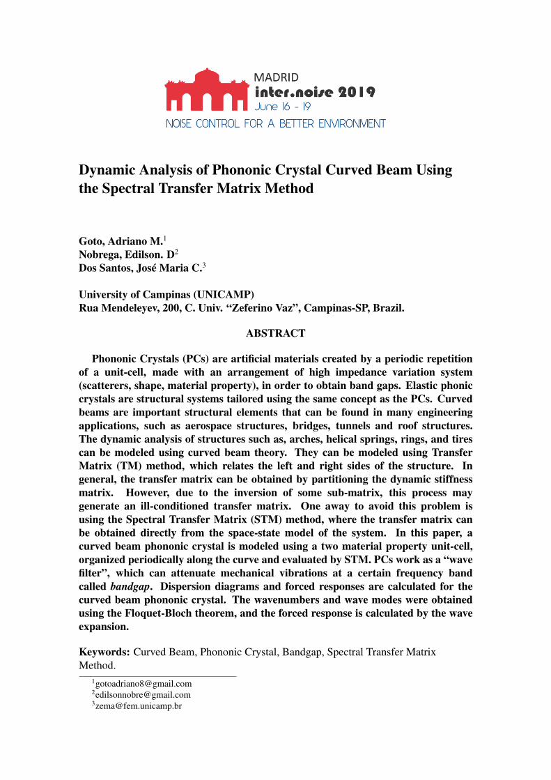
For a curved beam, the displacement and the internal forces can be rewritten inaccording to the radial and circumferential orientation. The curved beam model is acombination of elementary rod and Euler-Bernoulli beam theories. The straight beamlongitudinal and transversal displacements becomes circumferential and radial in thecurved beam, respectively, and the rotation remains the same. Figure 1 shows the in-planedisplacements () and internal forces of a curved beam.

Figure 1: Displacements and internal forces in a curved beam.

The coupled governing equation in frequency domain of a curved beam is given by[14, 1]: (

EA+EI

R2

)du

ds+ ρAω2 u+

1

R

(−EAdv

ds+ EI

d3v

ds3

)= 0,

EId4v

ds4+EA

R2v − ρAω2 v +

1

R

(−EAdu

ds+ EI

d3u

ds3

)= 0,

(4)

where u, v and are the cir is circumferential displacemente E,A, ρ, ω and I are,respectively, the Young’s modulus, cross-section area, mass density, circular frequencyand the moment of inertia. R indicates the curved beam radius.

The Equation 4 can be rewritten as:

d

ds

[EA

(du

ds− v

R

)]+EI

R

(d3v

ds3+

1

R

d2u

ds2

)+ ρAω2 u = 0

d

ds

[−EI

(d3v

ds3+

1

R

d2u

ds2

)]+EA

R

(du

ds− v

R

)+ ρAω2 v = 0

(5)

The internal forces and rotation are:

F = EA

(du

ds− v

R

)V = −EI

(d3v

ds3+

1

R

d2u

ds2

),

M = EI

(d2v

ds2+

1

R

du

ds

)ψ =

dv

ds.

(6)

The Equation 5 can be rewritten using the terms of internal forces, Equation 6, as:

du

ds=

v

R+

F

EA

dF

ds= −ρAω2 u+

V

R

dv

ds= ψ

dV

ds= −ρAω2 v − F

R

dψ

ds= − v

R2− F

REA+M

EI

dM

ds= −V

⇓

ddx

uvψFVM

=

0 1

R0 1

EA0 0

0 0 1 0 0 00 − 1

R2 0 − 1REA

0 1EI

−ρAω2 0 0 0 1R

00 −ρAω2 0 − 1

R0 0

0 0 0 0 −1 0

︸ ︷︷ ︸

G

uvψFVM

.

(7)

The transfer matrix is computed from Equation 3. This expression is showed in theAppendix.

3. MODELING OF ONE-DIMENSIONAL PHONONIC CRYSTALS

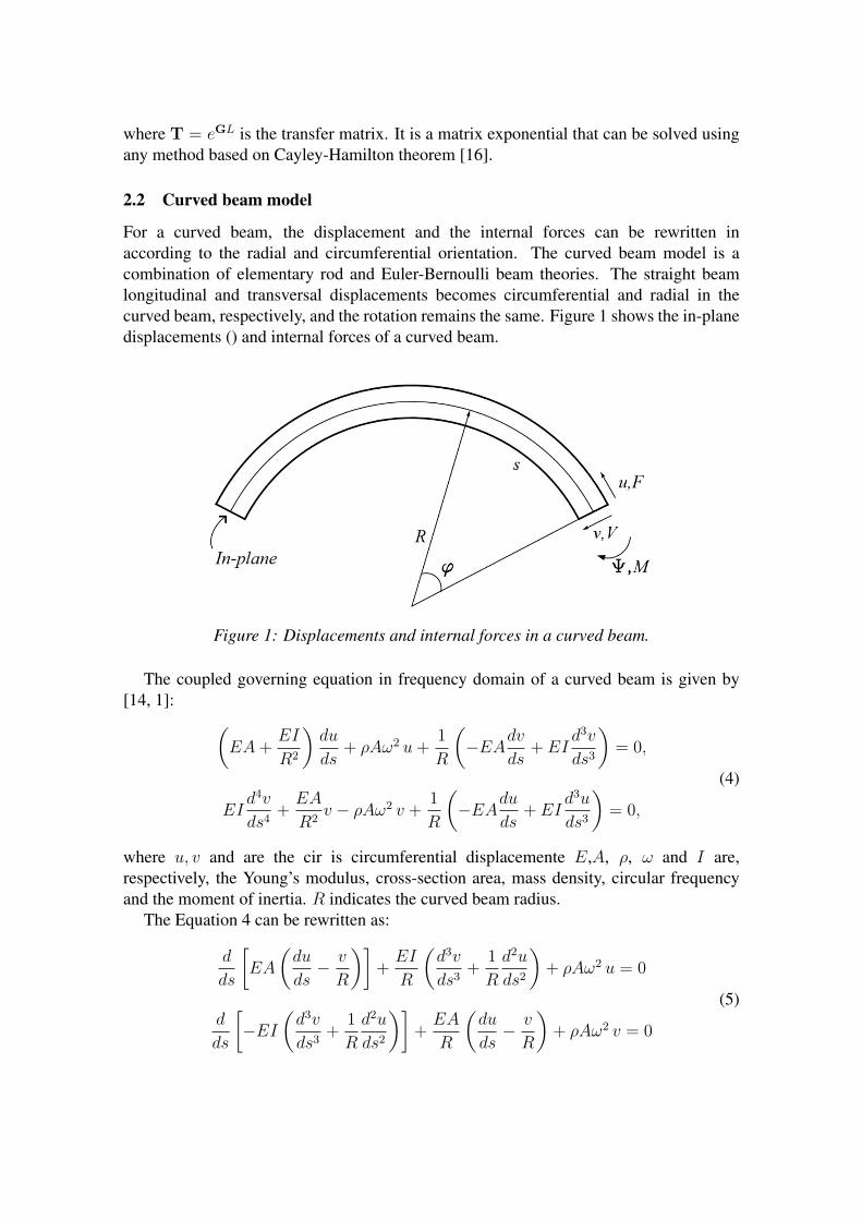
The phononic crystal (PC) unit cell contains two materials, which are polymer and steel.Figure 2 shows a schematic view of the phononic crystal and the unit-cell composed by asequence of polymer, steel and polymer.

For a 1D phononic crystal, the Equation 3 can be partitioned in terms of left and rightside of unit-cell as:

y(m)r = Tc y

(m)l , (8)

with the subscripts r and l corresponding to the right and left nodes of them−th unit-cell.While Tc represents Its transfer matrix, calculated by:

Tc = T1T2T1, (9)

where the subscript 1 and 2 indicates the polymer and steel proprieties, respectively.Using the coupling relation at the unit-cells interface ( y(m+1)

l = y(m)r ) and applying

Floquet-Bloch theorem [17] it has:

Tc y(m)l = e−i·kL y

(m)l or Tc yl = e−i·kL yl. (10)

The eigenproblem of Equation 9 is solved and the eigenvalues produces dispersiondiagrams and the eigenvectors the wave modes. It is important to note that the

Figure 2: Curved beam: phononic crystal unit-cell composed by polymer-steel-polymer.

eigenvectors and eigenvalues are independent of the unit-cell position in the structure.To each n degree of freedom has 2n eigenvalues that can be ordered appropriately intotwo groups: |eµj | ≤ 1, j = 1, 2, . . . , n indicate waves propagating to the right and|e−µ| ≥ 1, j = 1, 2, . . . , n correspond to waves traveling to the left. Therefore, waveamplitudes can be obtained as follows [18]:

y(m) =n∑j

e−i·kjLΦj y(m)j with m = 1, 2, 3 . . . Nc, Nc+1, (11)

where j = 1, 2, . . . , n with n as the number of eigenvalues and Nc the total number ofunit-cells.

4. NUMERICAL RESULTS

4.1 Validation of the STM method

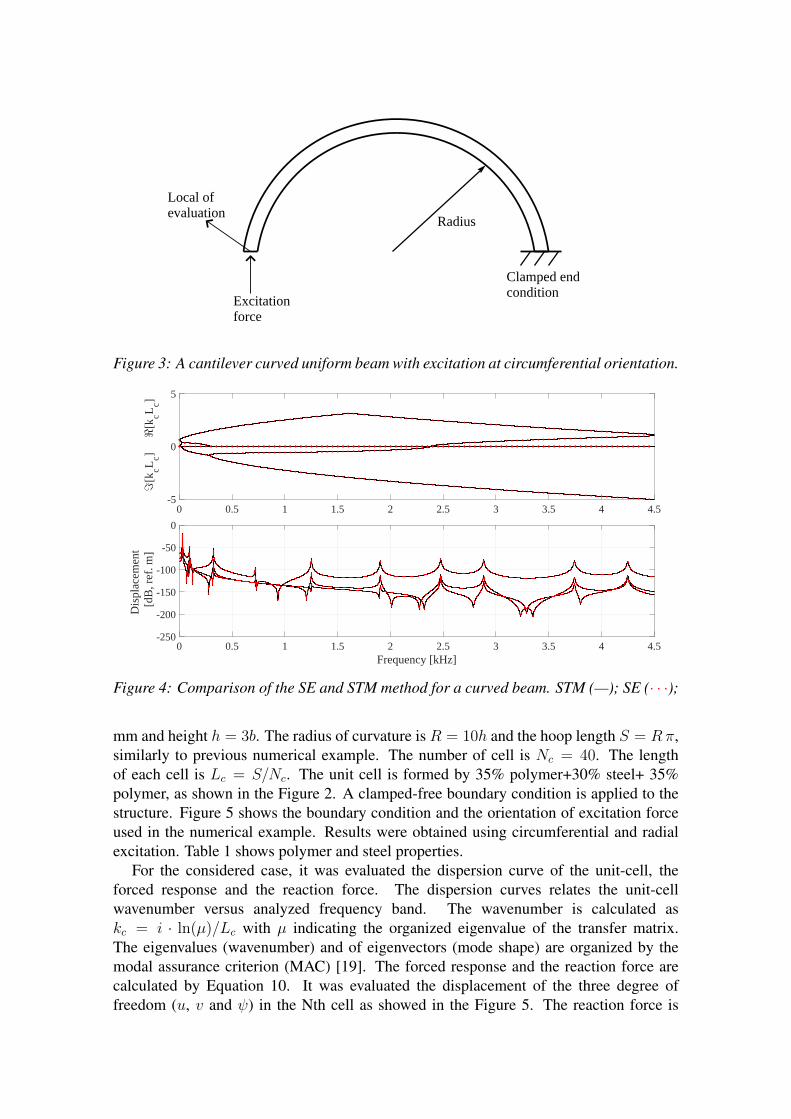
Initially, the STM method is compared with the Spectral Element (SE) method tovalidate the transfer matrix obtained for curved beam. It is considered a curved beam ofrectangular cross-sectional area of width b = 100 mm and height h = b/10. The radiusof curvature is R = 10h and the hoop length S = Rπ. The boundary conditions isshowed in the Figure 3. The structures was excited with unity force in the circumferentialdirection. The choice of the orientation force is arbitrary. The material propertiescorresponds to polymer with Young’s modulus E = 3 GPa, density ρ = 1340 kg m−3,Poisson’s ration ν = 0.4 and damping factor η = 0.002. Figure 4 shows the dispersioncurve and the forced response at the excitation point for a curved beam calculated bySTM and SE methods. The forced response is evaluated at the excitation point. As seen,the STM approach presents good agreement with the SE method. Particularly, the STMhas an advantage for not require the exact wave solution of the governing equation.

4.2 Analysis for PC curved beam

A numerical example of a phononic crystal curved beam with two different material isshowed. It is considered a curved beam of rectangular cross-sectional area of width b = 20

Radius

Excitationforce

Local ofevaluation

Clamped endcondition

Figure 3: A cantilever curved uniform beam with excitation at circumferential orientation.

0 0.5 1 1.5 2 2.5 3 3.5 4 4.5-5

0

5

[kcL

c]

[k

cLc]

0 0.5 1 1.5 2 2.5 3 3.5 4 4.5Frequency [kHz]

-250

-200

-150

-100

-50

0

Dis

plac

emen

t [

dB, r

ef. m

]

Figure 4: Comparison of the SE and STM method for a curved beam. STM (—); SE (· · ·);

mm and height h = 3b. The radius of curvature is R = 10h and the hoop length S = Rπ,similarly to previous numerical example. The number of cell is Nc = 40. The lengthof each cell is Lc = S/Nc. The unit cell is formed by 35% polymer+30% steel+ 35%polymer, as shown in the Figure 2. A clamped-free boundary condition is applied to thestructure. Figure 5 shows the boundary condition and the orientation of excitation forceused in the numerical example. Results were obtained using circumferential and radialexcitation. Table 1 shows polymer and steel properties.

For the considered case, it was evaluated the dispersion curve of the unit-cell, theforced response and the reaction force. The dispersion curves relates the unit-cellwavenumber versus analyzed frequency band. The wavenumber is calculated askc = i · ln(µ)/Lc with µ indicating the organized eigenvalue of the transfer matrix.The eigenvalues (wavenumber) and of eigenvectors (mode shape) are organized by themodal assurance criterion (MAC) [19]. The forced response and the reaction force arecalculated by Equation 10. It was evaluated the displacement of the three degree offreedom (u, v and ψ) in the Nth cell as showed in the Figure 5. The reaction force is

Figure 5: A cantilever PC curved beam with excitation in two different orientation.

Table 1: Phononic Crystal Material Properties.

Property Steel PolymerElastic Modulus [GPa] 210 3

Density [kg m−3] 8030 1340Poisson’s ratio 0.30 0.40Damping factor 0.001 0.002

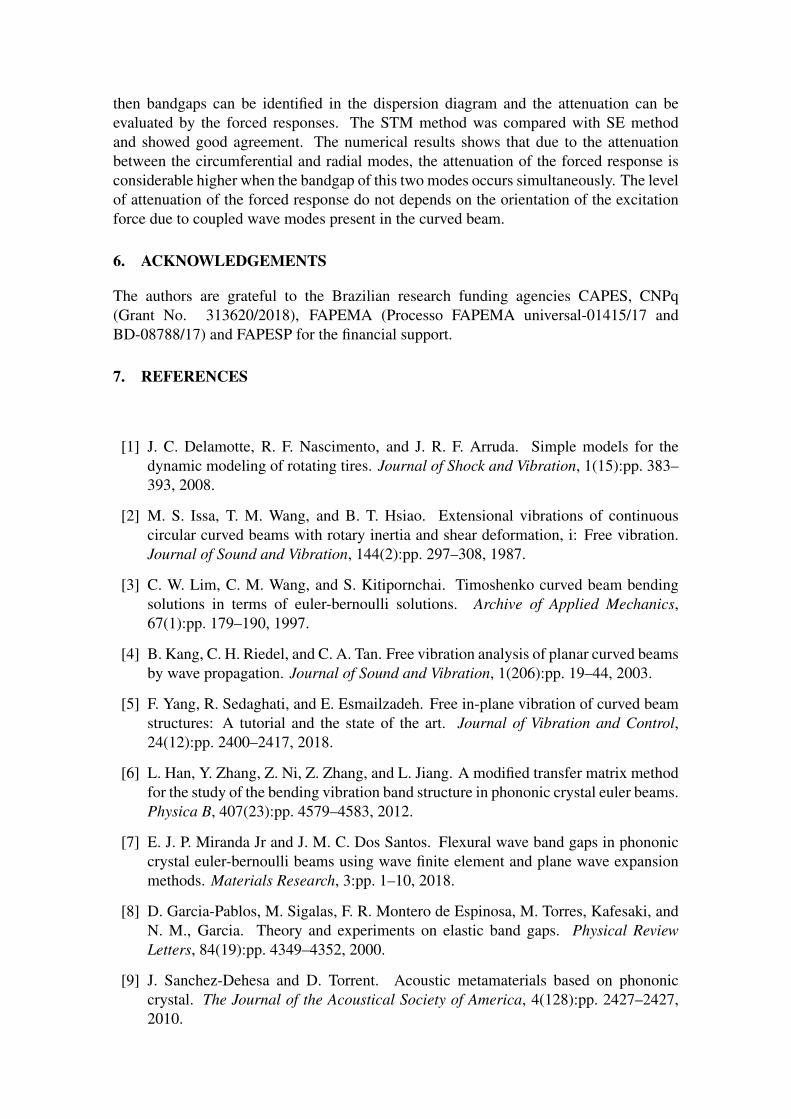
evaluated at the clamped end of the structure.Figure 6 shows the dispersion and receptance curves, respectively. In the graph

of dispersion curve, it can see that the curved beam considers propagation of threewave modes. The wavenumber is decomposed into real part (<[kcLc]) and imaginarypart (=[kcLc]). The bandgap region is indicated by the shaded areas. At the bandgapregion, the real part of wavenumber is equal to π or 0 (Bragg limit) while the imaginarypart has a non-zero value indicating a evanescent (non-propagating) wave behavior.As noted, both the circumferential and radial wave modes have two bandgap regionsindicated for light blue shaded and gray shaded areas, respectively. As seen in the Figure6, the receptance curve exposes a considered attenuation at the first circumferentialbandgap region (between 23.5-44.3 kHz). In this region the radial mode also presentsa bandgap. As can be noted, the circumferential and radial wave modes are relateditself. The attenuation only is significant with both circumferential and radial bandgapsare in the same frequency range. Another region where the bandgap modes intersectsitself is highlighted in the Figure 6 (between 121-122.4 kHz). Although the imaginarywavenumber part is small, in absolute values, the attenuation is considerable due to thecombination of circumferential and radial bandgap.

Figure 7 shows the transmittance curve. As seen, the attenuation behavior is similarto the first case shown in the Figure 6 where the decrease of transmittance values issignificantly higher when the two different bandgap occurs simultaneously. However,

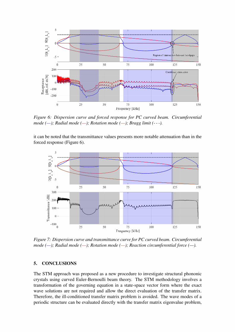
Figure 6: Dispersion curve and forced response for PC curved beam. Circumferentialmode (—); Radial mode (—); Rotation mode (—); Bragg limit (- - -).

it can be noted that the transmittance values presents more notable attenuation than in theforced response (Figure 6).

Figure 7: Dispersion curve and transmittance curve for PC curved beam. Circumferentialmode (—); Radial mode (—); Rotation mode (—); Reaction circumferential force (—).

5. CONCLUSIONS

The STM approach was proposed as a new procedure to investigate structural phononiccrystals using curved Euler-Bernoulli beam theory. The STM methodology involves atransformation of the governing equation in a state-space vector form where the exactwave solutions are not required and allow the direct evaluation of the transfer matrix.Therefore, the ill-conditioned transfer matrix problem is avoided. The wave modes of aperiodic structure can be evaluated directly with the transfer matrix eigenvalue problem,

then bandgaps can be identified in the dispersion diagram and the attenuation can beevaluated by the forced responses. The STM method was compared with SE methodand showed good agreement. The numerical results shows that due to the attenuationbetween the circumferential and radial modes, the attenuation of the forced response isconsiderable higher when the bandgap of this two modes occurs simultaneously. The levelof attenuation of the forced response do not depends on the orientation of the excitationforce due to coupled wave modes present in the curved beam.

6. ACKNOWLEDGEMENTS

The authors are grateful to the Brazilian research funding agencies CAPES, CNPq(Grant No. 313620/2018), FAPEMA (Processo FAPEMA universal-01415/17 andBD-08788/17) and FAPESP for the financial support.

7. REFERENCES

[1] J. C. Delamotte, R. F. Nascimento, and J. R. F. Arruda. Simple models for thedynamic modeling of rotating tires. Journal of Shock and Vibration, 1(15):pp. 383–393, 2008.

[2] M. S. Issa, T. M. Wang, and B. T. Hsiao. Extensional vibrations of continuouscircular curved beams with rotary inertia and shear deformation, i: Free vibration.Journal of Sound and Vibration, 144(2):pp. 297–308, 1987.

[3] C. W. Lim, C. M. Wang, and S. Kitipornchai. Timoshenko curved beam bendingsolutions in terms of euler-bernoulli solutions. Archive of Applied Mechanics,67(1):pp. 179–190, 1997.

[4] B. Kang, C. H. Riedel, and C. A. Tan. Free vibration analysis of planar curved beamsby wave propagation. Journal of Sound and Vibration, 1(206):pp. 19–44, 2003.

[5] F. Yang, R. Sedaghati, and E. Esmailzadeh. Free in-plane vibration of curved beamstructures: A tutorial and the state of the art. Journal of Vibration and Control,24(12):pp. 2400–2417, 2018.

[6] L. Han, Y. Zhang, Z. Ni, Z. Zhang, and L. Jiang. A modified transfer matrix methodfor the study of the bending vibration band structure in phononic crystal euler beams.Physica B, 407(23):pp. 4579–4583, 2012.

[7] E. J. P. Miranda Jr and J. M. C. Dos Santos. Flexural wave band gaps in phononiccrystal euler-bernoulli beams using wave finite element and plane wave expansionmethods. Materials Research, 3:pp. 1–10, 2018.

[8] D. Garcia-Pablos, M. Sigalas, F. R. Montero de Espinosa, M. Torres, Kafesaki, andN. M., Garcia. Theory and experiments on elastic band gaps. Physical ReviewLetters, 84(19):pp. 4349–4352, 2000.

[9] J. Sanchez-Dehesa and D. Torrent. Acoustic metamaterials based on phononiccrystal. The Journal of the Acoustical Society of America, 4(128):pp. 2427–2427,2010.

[10] T. J. R. Hughes. The finite element method: linear static and dynamic finite elementanalysis. Dover, 2000.

[11] J.-M. Mencik and M. Ichchou. Multi-mode propagation and diffusion in structuresthrough finite elements. European Journal of Mechanics - A/Solids, 5(24):pp. 877 –898, 2005.

[12] D. Duhamel, B. Mace, and M. Brennan. Finite element analysis of the vibrationsof waveguides and periodic structures. Journal of Sound and Vibration, 12(294):pp.205 – 220, 2006.

[13] E.D. Nobrega, F. Gautier, A. Pelat, and J.M.C. Dos Santos. Vibration band gaps forelastic metamaterial rods using wave finite element method. Mechanical Systemsand Signal Processing, (76):pp. 192–202, 2016.

[14] J.F. Doyle. Wave Propagation in Structures: Spectral Analysis Using Fast DiscreteFourier Transforms. Mechanical Engineering Series. Springer New York, 2012.

[15] U. Lee. Spectral Element Method in Structural Dynamics. Wiley, 2009.

[16] D. Rowell. Computing the matrix exponential - the cayley-hamilton method.

[17] D. J. Mead. A general theory of harmonic wave propagation in linear periodicsystems with multiple coupling. Journal of Sound and Vibration, 2(27):pp. 332–340, 1973.

[18] P. B. Silva, J.-M. Mencik, and Arruda. On the forced response of coupled systemsvia wfe based super-element approach. In Proceedings of ISMA, pages pp.1–13,2014.

[19] M. Pastor, M. Binda, and T. Harcarik. Modal assurance criterion. ProcediaEngineering, 1(48):pp. 543–548, 2012.

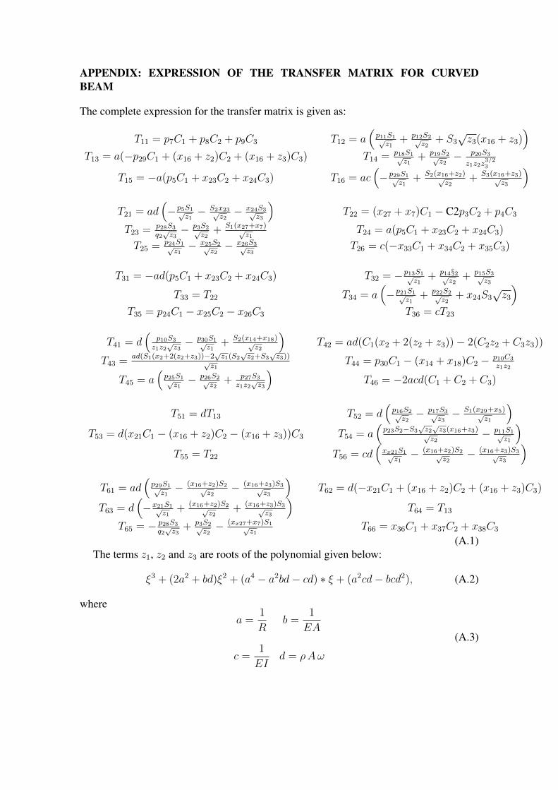
APPENDIX: EXPRESSION OF THE TRANSFER MATRIX FOR CURVEDBEAM

The complete expression for the transfer matrix is given as:

T11 = p7C1 + p8C2 + p9C3 T12 = a(p11S1√z1

+ p12S2√z2

+ S3√z3(x16 + z3)

)T13 = a(−p29C1 + (x16 + z2)C2 + (x16 + z3)C3) T14 = p18S1√

z1+ p19S2√

z2− p20S3

z1z2z3/23

T15 = −a(p5C1 + x23C2 + x24C3) T16 = ac(−p29S1√

z1+ S2(x16+z2)√

z2+ S3(x16+z3)√

z3

)T21 = ad

(−p5S1√

z1− S2x23√

z2− x24S3√

z3

)T22 = (x27 + x7)C1 − C2p3C2 + p4C3

T23 = p28S3

q2√z3− p3S2√

z2+ S1(x27+x7)√

z1T24 = a(p5C1 + x23C2 + x24C3)

T25 = p24S1√z1− x25S2√

z2− x26S3√

z3T26 = c(−x33C1 + x34C2 + x35C3)

T31 = −ad(p5C1 + x23C2 + x24C3) T32 = −p13S1√z1

+ p14§2√z2

+ p15S3√z3

T33 = T22 T34 = a(−p21S1√

z1+ p22S2√

z2+ x24S3

√z3

)T35 = p24C1 − x25C2 − x26C3 T36 = cT23

T41 = d(

p10S3

z1z2√z3− p30S1√

z1+ S2(x14+x18)√

z2

)T42 = ad(C1(x2 + 2(z2 + z3))− 2(C2z2 + C3z3))

T43 =ad(S1(x2+2(z2+z3))−2

√z1(S2

√z2+S3

√z3))√

z1T44 = p30C1 − (x14 + x18)C2 − p10C3

z1z2

T45 = a(p25S1√z1− p26S2√

z2+ p27S3

z1z2√z3

)T46 = −2acd(C1 + C2 + C3)

T51 = dT13 T52 = d(p16S2√z2− p17S3√

z3− S1(x29+x5)√

z1

)T53 = d(x21C1 − (x16 + z2)C2 − (x16 + z3))C3 T54 = a

(p23S2−S3

√z2√z3(x16+z3)√

z2− p11S1√

z1

)T55 = T22 T56 = cd

(xx21S1√

z1− (x16+z2)S2√

z2− (x16+z3)S3√

z3

)T61 = ad

(p29S1√z1− (x16+z2)S2√

z2− (x16+z3)S3√

z3

)T62 = d(−x21C1 + (x16 + z2)C2 + (x16 + z3)C3)

T63 = d(−x21S1√

z1+ (x16+z2)S2√

z2+ (x16+z3)S3√

z3

)T64 = T13

T65 = − p28S3

q2√z3

+ p3S2√z2− (xx27+x7)S1√

z1T66 = x36C1 + x37C2 + x38C3

(A.1)The terms z1, z2 and z3 are roots of the polynomial given below:

ξ3 + (2a2 + bd)ξ2 + (a4 − a2bd− cd) ∗ ξ + (a2cd− bcd2), (A.2)

wherea =

1

Rb =

1

EA

c =1

EId = ρAω

(A.3)

And the auxiliary terms used in the expressions are described in the A.4, A.5 and A.6:

x1 = a4 − (a2b+ c)d x2 = 4a2 + 2bdx3 = 2a2b+ c+ b2d x4 = a4 + 4a2bd+ b2d2

x5 = 5a4 + 4a2bd+ cd x6 = a4 + 6a2bdx7 = a4 + 2a2bd+ cd x8 = 4a8 − 2a6bd+ a2bcd2 − a4d(7c+ 2b2d)x9 = a4 + 5a2bd+ 3cd x10 = −a6 + a4bd+ a2cdx11 = −5a4 − a2bd+ cd x12 = 2a2b+ 2c+ b2d

x13 = z1z2 + (a2 − bd)(a2 + z3) x14 = a4 − a2bdx15 = a2 + 2bd+ z2 + z3 x16 = a2 − bd

x17 = a2 + 2bd x18 = (a2 + bd)z2 − z1z3x19 = (a2 + bd)z3 x20 = z2(a

2 + bd+ z3)x21 = 3a2 + z2 + z3 x22 = d(c+ 2b2d)

x23 = c− bz2 x24 = c− bz3x25 = bcd+ (a2b+ c)z2 x26 = bcd+ (a2b+ c)z3x27 = a2z3 + z2(a

2 + z3) x28 = a6 − a4bd− 2a2cd+ bcd2

x29 = 3a2z3 + z2(3a2 + z3) x30 = 3a4b+ b3d2 + a2(c+ 5b2d)

x31 = a2(−a2b+ c+ b2d) x32 = 3a4b+ bd(2c+ b2d) + a2(2c+ 5b2d)x33 = a2 + z2 + z3 x34 = a2 + bd+ z2x35 = a2 + bd+ z3 x36 = cd+ z2z3x37 = cd+ z1z3 x38 = cd+ z1z2

x39 = a2(13a2b+ 7c)d+ 2b(2a2b+ c)d2

(A.4)

p1 = x8 + (x9 + (7a2 + 2bd)z1)z22 p2 = z2(a

6 + x39 + x11z3)p3 = x1 + a2z2 − z1z3 p4 = x7 + a2z1 + (a2 + z1)z2p5 = x3 + b(z2 + z3) p6 = x10 + x11z1

p7 = z2(bd+ z3) + bd(x22

+ z3) p8 = −bdz2 + z1z3p9 = bd(x2

2+ z1) + (bd+ z1)z2 p10 = cd(z1z2 + x16(a

2 + z3))p11 = x22 + x6 + x17z3 + z2(x17 + z3) p12 = −x1 − x17z2 + z1z3

p13 = a2(4cd+ 2b2d2 + x6) + x7z3 + z2(x7 + a2z3) p14 = x28 + x7z2 − a2z1z3p15 = cdx16 + z3(−x1 − a2z3) p16 = x1 + 3a2z2 − z1z3p17 = x5 + 3a2z1 + (3a2 + z1)z2 p18 = x30 + 1

2bx2z3 + bz2(

x2x

+ z3)p19 = x31 − 1

2bx2z2 + bz1z3 p20 = cdx16(a

2c− bcd+ bz23)p21 = x32 + x3z3 + z2(x3 + bz3) p22 = bx1 + x3z2 − bz1z3

p23 = x1 + x17z2 − z1z3 p24 = a2x12 + (a2b+ c)(z2 + z3)p25 = 2cd+ x19 + x20 + x4 p26 = −2cd+ x14 + x18p27 = cd(z1z2 − x16(a2 + z3)) p28 = p1 + p2 + 3z1z

32 + p6z3

p29 = x17 + z2 + z3 p30 = x19 + x20 + x4(A.5)

q1 = x1 + z1(x2 + 3z1) q2 = x1 + z2(x2 + 3z2) q3 = x1 + z3(x2 + 3z3) (A.6)