Embed Size (px)
Citation preview

The Vasicek interest rate modelThe CIR interest rate model
Numerical example: Vasicek vs. CIRTwo-factor Vasicek model
Dynamic Asset AllocationChapter 10: Stochastic interest rates
Claus Munk
August 2012
AARHUS UNIVERSITY AU
1 / 41
The Vasicek interest rate modelThe CIR interest rate model
Numerical example: Vasicek vs. CIRTwo-factor Vasicek model
Motivation
• Interest rates and bond yields vary stochastically over time include short-term interest rate rt as state variable
• Obtain explicit solutions for affine short-rate models, e.g.I Vasicek model (1977)I CIR model (1985)
• Investors are concerned about real interest rates want toinvest in real bonds
• Determine the optimal bond/stock mixI assume single stock is traded (stock index); can be generalized
• Investors with non-log utility will hedge variations in interest rates• Bonds carry a build-in hedge against interest rate risk: bond
prices are inversely related to interest rates• Look at the consequences for an investor if he follows a
suboptimal investment strategy in the Vasicek world
2 / 41
The Vasicek interest rate modelThe CIR interest rate model
Numerical example: Vasicek vs. CIRTwo-factor Vasicek model
Outline
1 The Vasicek interest rate model
2 The CIR interest rate model
3 Numerical example: Vasicek vs. CIR
4 Two-factor Vasicek model
3 / 41
The Vasicek interest rate modelThe CIR interest rate model
Numerical example: Vasicek vs. CIRTwo-factor Vasicek model
The modelOptimal strategies with CRRA utilityNumerical exampleSuboptimal strategies with Vasicek model
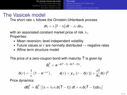
The Vasicek modelThe short rate rt follows the Ornstein-Uhlenbeck process
drt = κ [r − rt ] dt − σr dz1t
with an associated constant market price of risk λ1.Properties:• Mean reversion; level-independent volatility• Future values or r are normally distributed negative rates• Affine term structure model
The price of a zero-coupon bond with maturity T is given by
BTt = e−a(T−t)−b(T−t)rt ,
b(τ) =1κ
(1− e−κτ
), a(τ) = y∞ (τ − b(τ)) +
σ2r
4κb(τ)2
Price dynamics
dBTt = BT
t[(
rt + λ1σr b(T − t))
dt + σr b(T − t)dz1t]
6 / 41
The Vasicek interest rate modelThe CIR interest rate model
Numerical example: Vasicek vs. CIRTwo-factor Vasicek model
The modelOptimal strategies with CRRA utilityNumerical exampleSuboptimal strategies with Vasicek model
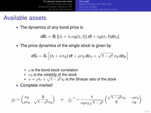
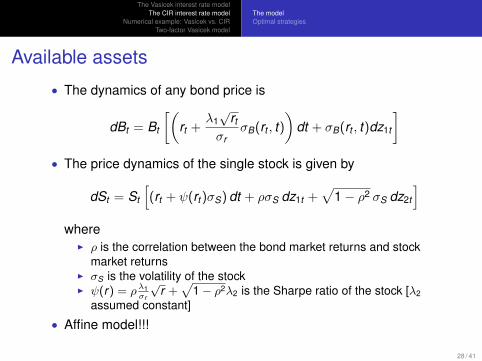
Available assets• The dynamics of any bond price is
dBt = Bt [(rt + λ1σB(rt , t)) dt + σB(rt , t)dz1t ]
• The price dynamics of the single stock is given by
dSt = St
[(rt + ψσS) dt + ρσS dz1t +
√1− ρ2 σS dz2t
]I ρ is the bond-stock correlationI σS is the volatility of the stockI ψ = ρλ1 +
√1− ρ2λ2 is the Sharpe ratio of the stock
• Complete market!
σ t =
(σB 0ρσS
√1− ρ2σS
)⇒ σ−1
t =1
σBσS
√1− ρ2
(√1− ρ2σS −ρσS
0 σB
)7 / 41

The Vasicek interest rate modelThe CIR interest rate model
Numerical example: Vasicek vs. CIRTwo-factor Vasicek model
The modelOptimal strategies with CRRA utilityNumerical exampleSuboptimal strategies with Vasicek model
Affine model...The model falls in the affine framework of Sec. 7.3.2.
A′1(τ) = 1− κA1(τ), A1(0) = 0
has the solution
A1(τ) =1κ
(1− e−κτ
)= b(τ).
A0(τ) =1
2γ
(λ2
1 + λ22
)τ +
(κr +
γ − 1γ
σrλ1
)∫ τ
0b(s) ds − γ − 1
2γσ2
r
∫ τ
0b(s)2 ds
=1
2γ
(λ2
1 + λ22
)τ +
(r − γ − 1
2κ2γ
[σ2
r − 2κσrλ1
])(τ − b(τ)) +
γ − 14κγ
σ2r b(τ)2,
using∫ τ
0b(s) ds =
1κ
(τ − b(τ)) ,
∫ τ
0b(s)2 ds =
1κ2 (τ − b(τ))− 1
2κb(τ)2.
9 / 41
The Vasicek interest rate modelThe CIR interest rate model
Numerical example: Vasicek vs. CIRTwo-factor Vasicek model
The modelOptimal strategies with CRRA utilityNumerical exampleSuboptimal strategies with Vasicek model
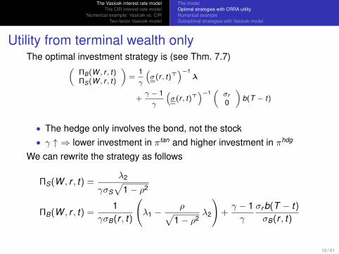
Utility from terminal wealth onlyThe optimal investment strategy is (see Thm. 7.7)(
ΠB(W , r , t)ΠS(W , r , t)
)=
1γ
(σ (r , t)>
)−1λ
+γ − 1γ
(σ (r , t)>
)−1(
σr0
)b(T − t)
• The hedge only involves the bond, not the stock• γ ↑ ⇒ lower investment in πtan and higher investment in πhdg
We can rewrite the strategy as follows
ΠS(W , r , t) =λ2
γσS√
1− ρ2
ΠB(W , r , t) =1
γσB(r , t)
(λ1 −
ρ√1− ρ2
λ2
)+γ − 1γ
σr b(T − t)σB(r , t)
10 / 41
The Vasicek interest rate modelThe CIR interest rate model
Numerical example: Vasicek vs. CIRTwo-factor Vasicek model
The modelOptimal strategies with CRRA utilityNumerical exampleSuboptimal strategies with Vasicek model
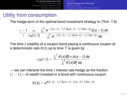
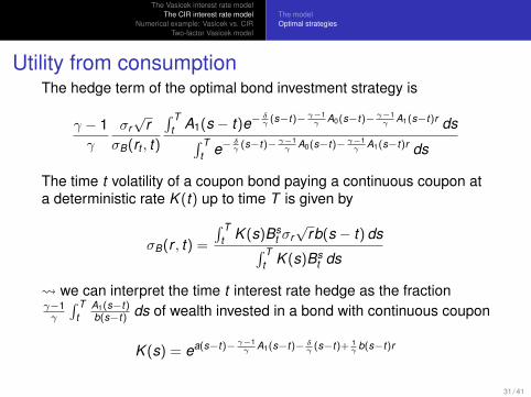
Utility from consumptionThe hedge term of the optimal bond investment strategy is (Thm. 7.8)
γ − 1γ
σr
σB(rt , t)
∫ Tt e−
δγ (s−t)− γ−1
γ A0(s−t)− γ−1γ b(s−t)r b(s − t) ds∫ T
t e−δγ (s−t)− γ−1
γ A0(s−t)− γ−1γ b(s−t)r ds
The time t volatility of a coupon bond paying a continuous coupon ata deterministic rate K (t) up to time T is given by
σB(r , t) =
∫ Tt K (s)Bs
t σr b(s − t) ds∫ Tt K (s)Bs
t ds
we can interpret the time t interest rate hedge as the fraction(γ − 1)/γ of wealth invested in a bond with continuous coupon
K (s) = ea(s−t)− γ−1γ A0(s−t)− δ
γ (s−t)+ 1γ b(s−t)r
11 / 41
The Vasicek interest rate modelThe CIR interest rate model
Numerical example: Vasicek vs. CIRTwo-factor Vasicek model
The modelOptimal strategies with CRRA utilityNumerical exampleSuboptimal strategies with Vasicek model
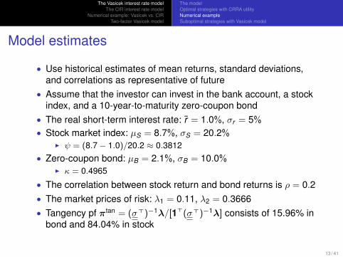
Model estimates
• Use historical estimates of mean returns, standard deviations,and correlations as representative of future
• Assume that the investor can invest in the bank account, a stockindex, and a 10-year-to-maturity zero-coupon bond
• The real short-term interest rate: r = 1.0%, σr = 5%
• Stock market index: µS = 8.7%, σS = 20.2%I ψ = (8.7− 1.0)/20.2 ≈ 0.3812
• Zero-coupon bond: µB = 2.1%, σB = 10.0%I κ = 0.4965
• The correlation between stock return and bond returns is ρ = 0.2• The market prices of risk: λ1 = 0.11, λ2 = 0.3666• Tangency pf πtan = (σ>)−1λ/[1>(σ>)−1λ] consists of 15.96% in
bond and 84.04% in stock
13 / 41
The Vasicek interest rate modelThe CIR interest rate model
Numerical example: Vasicek vs. CIRTwo-factor Vasicek model
The modelOptimal strategies with CRRA utilityNumerical exampleSuboptimal strategies with Vasicek model
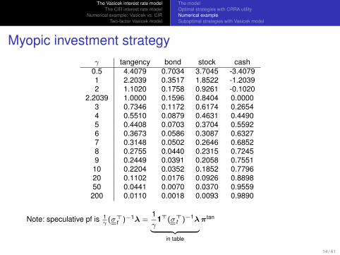
Myopic investment strategyγ tangency bond stock cash
0.5 4.4079 0.7034 3.7045 -3.40791 2.2039 0.3517 1.8522 -1.20392 1.1020 0.1758 0.9261 -0.1020
2.2039 1.0000 0.1596 0.8404 0.00003 0.7346 0.1172 0.6174 0.26544 0.5510 0.0879 0.4631 0.44905 0.4408 0.0703 0.3704 0.55926 0.3673 0.0586 0.3087 0.63277 0.3148 0.0502 0.2646 0.68528 0.2755 0.0440 0.2315 0.72459 0.2449 0.0391 0.2058 0.755110 0.2204 0.0352 0.1852 0.779620 0.1102 0.0176 0.0926 0.889850 0.0441 0.0070 0.0370 0.9559
200 0.0110 0.0018 0.0093 0.9890
Note: speculative pf is 1γ
(σ>t )−1λ =
1γ
1>(σ>t )−1λ︸ ︷︷ ︸
in table
πtan
14 / 41
The Vasicek interest rate modelThe CIR interest rate model
Numerical example: Vasicek vs. CIRTwo-factor Vasicek model
The modelOptimal strategies with CRRA utilityNumerical exampleSuboptimal strategies with Vasicek model
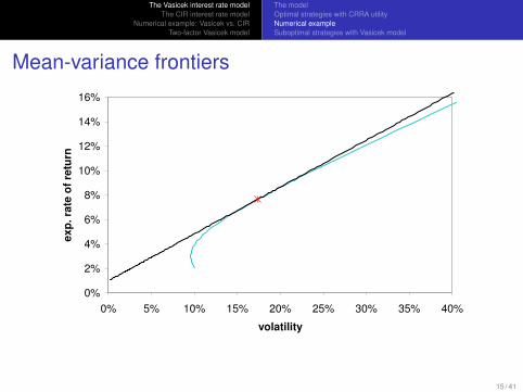
Mean-variance frontiers
0%
2%
4%
6%
8%
10%
12%
14%
16%
0% 5% 10% 15% 20% 25% 30% 35% 40%
volatility
ex
p.
rate
of
retu
rn
15 / 41
The Vasicek interest rate modelThe CIR interest rate model
Numerical example: Vasicek vs. CIRTwo-factor Vasicek model
The modelOptimal strategies with CRRA utilityNumerical exampleSuboptimal strategies with Vasicek model
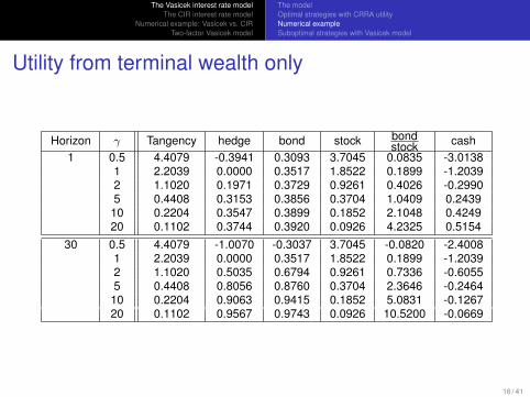
Utility from terminal wealth only
Horizon γ Tangency hedge bond stock bondstock cash
1 0.5 4.4079 -0.3941 0.3093 3.7045 0.0835 -3.01381 2.2039 0.0000 0.3517 1.8522 0.1899 -1.20392 1.1020 0.1971 0.3729 0.9261 0.4026 -0.29905 0.4408 0.3153 0.3856 0.3704 1.0409 0.243910 0.2204 0.3547 0.3899 0.1852 2.1048 0.424920 0.1102 0.3744 0.3920 0.0926 4.2325 0.5154
30 0.5 4.4079 -1.0070 -0.3037 3.7045 -0.0820 -2.40081 2.2039 0.0000 0.3517 1.8522 0.1899 -1.20392 1.1020 0.5035 0.6794 0.9261 0.7336 -0.60555 0.4408 0.8056 0.8760 0.3704 2.3646 -0.246410 0.2204 0.9063 0.9415 0.1852 5.0831 -0.126720 0.1102 0.9567 0.9743 0.0926 10.5200 -0.0669
16 / 41
The Vasicek interest rate modelThe CIR interest rate model
Numerical example: Vasicek vs. CIRTwo-factor Vasicek model
The modelOptimal strategies with CRRA utilityNumerical exampleSuboptimal strategies with Vasicek model
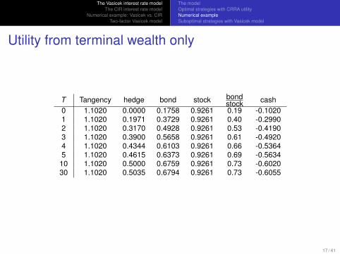
Utility from terminal wealth only
T Tangency hedge bond stock bondstock cash
0 1.1020 0.0000 0.1758 0.9261 0.19 -0.10201 1.1020 0.1971 0.3729 0.9261 0.40 -0.29902 1.1020 0.3170 0.4928 0.9261 0.53 -0.41903 1.1020 0.3900 0.5658 0.9261 0.61 -0.49204 1.1020 0.4344 0.6103 0.9261 0.66 -0.53645 1.1020 0.4615 0.6373 0.9261 0.69 -0.563410 1.1020 0.5000 0.6759 0.9261 0.73 -0.602030 1.1020 0.5035 0.6794 0.9261 0.73 -0.6055
17 / 41
The Vasicek interest rate modelThe CIR interest rate model
Numerical example: Vasicek vs. CIRTwo-factor Vasicek model
The modelOptimal strategies with CRRA utilityNumerical exampleSuboptimal strategies with Vasicek model
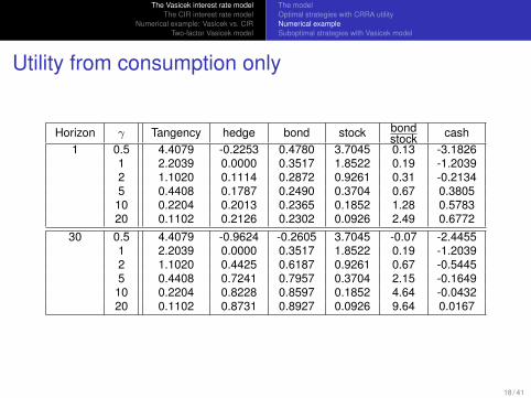
Utility from consumption only
Horizon γ Tangency hedge bond stock bondstock cash
1 0.5 4.4079 -0.2253 0.4780 3.7045 0.13 -3.18261 2.2039 0.0000 0.3517 1.8522 0.19 -1.20392 1.1020 0.1114 0.2872 0.9261 0.31 -0.21345 0.4408 0.1787 0.2490 0.3704 0.67 0.3805
10 0.2204 0.2013 0.2365 0.1852 1.28 0.578320 0.1102 0.2126 0.2302 0.0926 2.49 0.6772
30 0.5 4.4079 -0.9624 -0.2605 3.7045 -0.07 -2.44551 2.2039 0.0000 0.3517 1.8522 0.19 -1.20392 1.1020 0.4425 0.6187 0.9261 0.67 -0.54455 0.4408 0.7241 0.7957 0.3704 2.15 -0.1649
10 0.2204 0.8228 0.8597 0.1852 4.64 -0.043220 0.1102 0.8731 0.8927 0.0926 9.64 0.0167
18 / 41
The Vasicek interest rate modelThe CIR interest rate model
Numerical example: Vasicek vs. CIRTwo-factor Vasicek model
The modelOptimal strategies with CRRA utilityNumerical exampleSuboptimal strategies with Vasicek model
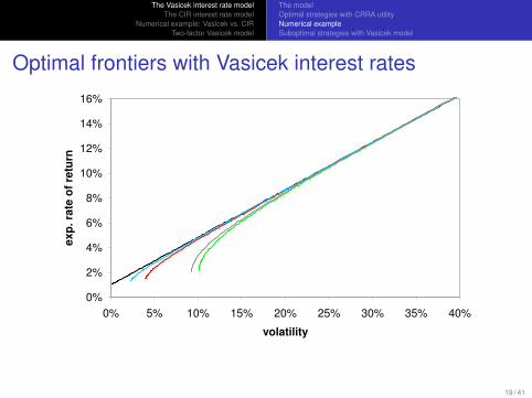
Optimal frontiers with Vasicek interest rates
0%
2%
4%
6%
8%
10%
12%
14%
16%
0% 5% 10% 15% 20% 25% 30% 35% 40%
volatility
ex
p.
rate
of
retu
rn
19 / 41
The Vasicek interest rate modelThe CIR interest rate model
Numerical example: Vasicek vs. CIRTwo-factor Vasicek model
The modelOptimal strategies with CRRA utilityNumerical exampleSuboptimal strategies with Vasicek model
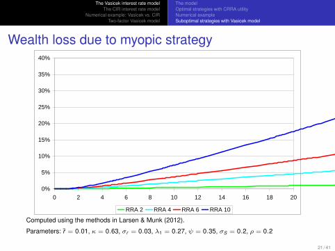
Wealth loss due to myopic strategy
0%
5%
10%
15%
20%
25%
30%
35%
40%
0 2 4 6 8 10 12 14 16 18 20
RRA 2 RRA 4 RRA 6 RRA 10
Computed using the methods in Larsen & Munk (2012).
Parameters: r = 0.01, κ = 0.63, σr = 0.03, λ1 = 0.27, ψ = 0.35, σS = 0.2, ρ = 0.2
21 / 41
The Vasicek interest rate modelThe CIR interest rate model
Numerical example: Vasicek vs. CIRTwo-factor Vasicek model
The modelOptimal strategies with CRRA utilityNumerical exampleSuboptimal strategies with Vasicek model
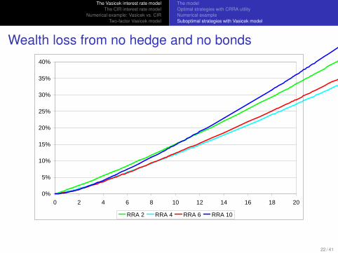
Wealth loss from no hedge and no bonds
0%
5%
10%
15%
20%
25%
30%
35%
40%
0 2 4 6 8 10 12 14 16 18 20
RRA 2 RRA 4 RRA 6 RRA 10
22 / 41
The Vasicek interest rate modelThe CIR interest rate model
Numerical example: Vasicek vs. CIRTwo-factor Vasicek model
The modelOptimal strategies with CRRA utilityNumerical exampleSuboptimal strategies with Vasicek model
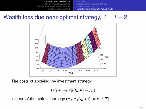
Wealth loss due near-optimal strategy, T − t = 2
-0,25 -0,15 -0,05 0,05 0,15 0,25 0,35 0,45-0,5
-0,35
-0,2
-0,05
0,1
0,25
0%
1%
2%
3%
4%
5%
6%
7%
PhiS
PhiB
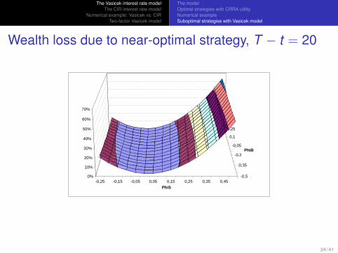
The costs of applying the investment strategy
(π∗S + ϕS, π∗B(ru,u) + ϕB)
instead of the optimal strategy (π∗S, π∗B(ru,u)) over [t ,T ].
23 / 41
The Vasicek interest rate modelThe CIR interest rate model
Numerical example: Vasicek vs. CIRTwo-factor Vasicek model
The modelOptimal strategies with CRRA utilityNumerical exampleSuboptimal strategies with Vasicek model
Wealth loss due to near-optimal strategy, T − t = 20
-0,25 -0,15 -0,05 0,05 0,15 0,25 0,35 0,45-0,5
-0,35
-0,2
-0,05
0,1
0,25
0%
10%
20%
30%
40%
50%
60%
70%
PhiS
PhiB
24 / 41
The Vasicek interest rate modelThe CIR interest rate model
Numerical example: Vasicek vs. CIRTwo-factor Vasicek model
The modelOptimal strategies
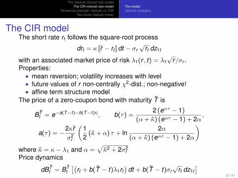
The CIR modelThe short rate rt follows the square-root process
drt = κ [r − rt ] dt − σr√
rt dz1t
with an associated market price of risk λ1(r , t) = λ1√
r/σr .Properties:• mean reversion; volatility increases with level• future values of r non-centrally χ2-dist.; non-negative!• affine term structure model
The price of a zero-coupon bond with maturity T is
BTt = e−a(T−t)−b(T−t)rt , b(τ) =
2 (eατ − 1)
(α + κ) (eατ − 1) + 2α,
a(τ) = −2κrσ2
r
(12
(κ+ α) τ + ln2α
(α + κ) (eατ − 1) + 2α
)where κ = κ− λ1 and α =
√κ2 + 2σ2
rPrice dynamics
dBTt = BT
t[(
rt + b(T − t)λ1rt)
dt + b(T − t)σr√
rt dz1t]
27 / 41
The Vasicek interest rate modelThe CIR interest rate model
Numerical example: Vasicek vs. CIRTwo-factor Vasicek model
The modelOptimal strategies
Available assets
• The dynamics of any bond price is
dBt = Bt
[(rt +
λ1√
rt
σrσB(rt , t)
)dt + σB(rt , t)dz1t
]• The price dynamics of the single stock is given by
dSt = St
[(rt + ψ(rt )σS) dt + ρσS dz1t +
√1− ρ2 σS dz2t
]where
I ρ is the correlation between the bond market returns and stockmarket returns
I σS is the volatility of the stockI ψ(r) = ρλ1
σr
√r +
√1− ρ2λ2 is the Sharpe ratio of the stock [λ2
assumed constant]
• Affine model!!!
28 / 41
The Vasicek interest rate modelThe CIR interest rate model
Numerical example: Vasicek vs. CIRTwo-factor Vasicek model
The modelOptimal strategies
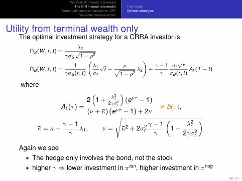
Utility from terminal wealth onlyThe optimal investment strategy for a CRRA investor is
ΠS(W , r , t) =λ2
γσS√
1− ρ2
ΠB(W , r , t) =1
γσB(r , t)
(λ1
σr
√r −
ρ√1− ρ2
λ2
)+γ − 1γ
σr√
rσB(r , t)
A1(T − t)
where
A1(τ) =2(
1 +λ2
12γσ2
r
)(eντ − 1)
(ν + κ) (eντ − 1) + 2ν6= b(τ),
κ = κ− γ − 1γ
λ1, ν =
√κ2 + 2σ2
rγ − 1γ
(1 +
λ21
2γσ2r
).
Again we see• The hedge only involves the bond, not the stock• higher γ ⇒ lower investment in πtan, higher investment in πhdg
30 / 41
The Vasicek interest rate modelThe CIR interest rate model
Numerical example: Vasicek vs. CIRTwo-factor Vasicek model
The modelOptimal strategies
Utility from consumptionThe hedge term of the optimal bond investment strategy is
γ − 1γ
σr√
rσB(rt , t)
∫ Tt A1(s − t)e−
δγ (s−t)− γ−1
γ A0(s−t)− γ−1γ A1(s−t)r ds∫ T
t e−δγ (s−t)− γ−1
γ A0(s−t)− γ−1γ A1(s−t)r ds
The time t volatility of a coupon bond paying a continuous coupon ata deterministic rate K (t) up to time T is given by
σB(r , t) =
∫ Tt K (s)Bs
t σr√
rb(s − t) ds∫ Tt K (s)Bs
t ds
we can interpret the time t interest rate hedge as the fractionγ−1γ
∫ Tt
A1(s−t)b(s−t) ds of wealth invested in a bond with continuous coupon
K (s) = ea(s−t)− γ−1γ A1(s−t)− δ
γ (s−t)+ 1γ b(s−t)r
31 / 41
The Vasicek interest rate modelThe CIR interest rate model
Numerical example: Vasicek vs. CIRTwo-factor Vasicek model
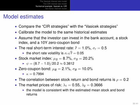
Model estimates
• Compare the “CIR strategies” with the “Vasicek strategies”• Calibrate the model to the same historical estimates• Assume that the investor can invest in the bank account, a stock
index, and a 10Y zero-coupon bond• The real short-term interest rate: r = 1.0%, σr = 0.5
I the short rate volatility is σr√
r = 0.05• Stock market index: µS = 8.7%, σS = 20.2%
I ψ = (8.7− 1.0)/20.2 ≈ 0.3812• Zero-coupon bond: µB = 2.1%, σB = 10.0%
I κ = 0.7994
• The correlation between stock return and bond returns is ρ = 0.2• The market prices of risk: λ1 = 0.55, λ2 = 0.3666
I the model is consistent with the estimated mean stock and bondreturns
33 / 41
The Vasicek interest rate modelThe CIR interest rate model
Numerical example: Vasicek vs. CIRTwo-factor Vasicek model
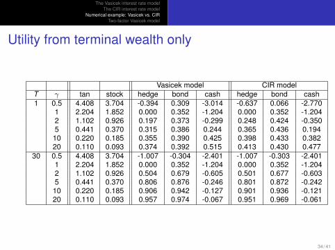
Utility from terminal wealth only
Vasicek model CIR modelT γ tan stock hedge bond cash hedge bond cash1 0.5 4.408 3.704 -0.394 0.309 -3.014 -0.637 0.066 -2.770
1 2.204 1.852 0.000 0.352 -1.204 0.000 0.352 -1.2042 1.102 0.926 0.197 0.373 -0.299 0.248 0.424 -0.3505 0.441 0.370 0.315 0.386 0.244 0.365 0.436 0.19410 0.220 0.185 0.355 0.390 0.425 0.398 0.433 0.38220 0.110 0.093 0.374 0.392 0.515 0.413 0.430 0.477
30 0.5 4.408 3.704 -1.007 -0.304 -2.401 -1.007 -0.303 -2.4011 2.204 1.852 0.000 0.352 -1.204 0.000 0.352 -1.2042 1.102 0.926 0.504 0.679 -0.605 0.501 0.677 -0.6035 0.441 0.370 0.806 0.876 -0.246 0.801 0.872 -0.24210 0.220 0.185 0.906 0.942 -0.127 0.901 0.936 -0.12120 0.110 0.093 0.957 0.974 -0.067 0.951 0.969 -0.061
34 / 41
The Vasicek interest rate modelThe CIR interest rate model
Numerical example: Vasicek vs. CIRTwo-factor Vasicek model
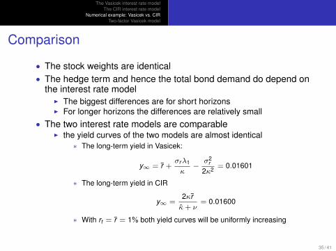
Comparison
• The stock weights are identical• The hedge term and hence the total bond demand do depend on
the interest rate modelI The biggest differences are for short horizonsI For longer horizons the differences are relatively small
• The two interest rate models are comparableI the yield curves of the two models are almost identical
∗ The long-term yield in Vasicek:
y∞ = r +σrλ1
κ−
σ2r
2κ2= 0.01601
∗ The long-term yield in CIR
y∞ =2κrκ+ ν
= 0.01600
∗ With rt = r = 1% both yield curves will be uniformly increasing
35 / 41
The Vasicek interest rate modelThe CIR interest rate model
Numerical example: Vasicek vs. CIRTwo-factor Vasicek model
Model
drt = (ϕr + ut − κr rt ) dt − σr dz1t ,
dut = −κuut dt − σuρru dz1t − σu
√1− ρ2
ru dz2t ,
and constant market prices of risk λ1, λ2.Zero-coupon bond prices
BT (r , u, t) = e−a(T−t)−b1(T−t)r−b2(T−t)u ,
where
b1(τ) =1κr
(1− e−κr τ
), b2(τ) =
1κrκu
+1
κr (κr − κu)e−κr τ −
1κu(κr − κu)
e−κuτ ,
a(τ) = complicated and less important
Bond price dynamics
dBTt = BT
t
[(rt + ψB(T − t)
)dt + σB1(T − t) dz1t + σB2(T − t) dz2t
],
where, for all τ ≥ 0, we have defined
ψB(τ) = λ1σB1(τ) + λ2σB2(τ),
σB1(τ) = σr b1(τ) + σuρrub2(τ), σB2(τ) = σu
√1− ρ2
rub2(τ).
37 / 41
The Vasicek interest rate modelThe CIR interest rate model
Numerical example: Vasicek vs. CIRTwo-factor Vasicek model
Asset allocationIndividual with CRRA utility of terminal wealth, who can invest in
1 the locally risk-free asset (=bank account; cash deposits) with rate of return rt ,
2 a zero-coupon bond maturing at time T1,
3 a zero-coupon bond maturing at time T2 6= T1,
4 the stock with
dSt = St [(rt + ψSσS) dt + σSk1 dz1t + σSk2 dz2t + σSk3 dz3t ] .
Two-dimensional affine asset allocation model
J(W , r , u, t) =1
1− γg(r , u, t)γW 1−γ ,
g(r , u, t) = exp{−γ − 1γ
A0(T − t)−γ − 1γ
A1r (T − t)r −γ − 1γ
A1u(T − t)u},
A1r (τ) ≡ b1(τ), A1u(τ) ≡ b2(τ).
Optimal investment strategy isπB1(t)πB2(t)πS
=1γ
(σ (t)>
)−1λ−
γ − 1γ
(σ (t)>
)−1
−σr −σuρru
0 −σu
√1− ρ2
ru0 0
(A1r (T − t)A1u(T − t)
)
38 / 41
The Vasicek interest rate modelThe CIR interest rate model
Numerical example: Vasicek vs. CIRTwo-factor Vasicek model
The optimal investment in the stock reduces to
πS =1γ
λ3
σSk3.
The optimal investments in the two bonds can be rewritten as
πB1(t) =1
γσrσu
√1− ρ2
rud(t)
(σr b1(T2 − t)
[k2λ3
k3− λ2
]
+ σub2(T2 − t)[(λ1 −
k1λ3
k3
)√1− ρ2
ru +
(k2λ3
k3− λ2
)ρru
])
+γ − 1γd(t)
(b2(T2 − t)b1(T − t)− b1(T2 − t)b2(T − t)) ,
πB2(t) =1
γσrσu
√1− ρ2
rud(t)
(σr b1(T1 − t)
[λ2 −
k2λ3
k3
]
+ σub2(T1 − t)[(
k1λ3
k3− λ1
)√1− ρ2
ru +
(λ2 −
k2λ3
k3
)ρru
])
+γ − 1γd(t)
(b1(T1 − t)b2(T − t)− b1(T − t)b2(T1 − t)) ,
whered(t) = b1(T1 − t)b2(T2 − t)− b1(T2 − t)b2(T1 − t).
39 / 41
The Vasicek interest rate modelThe CIR interest rate model
Numerical example: Vasicek vs. CIRTwo-factor Vasicek model
Optimal portfolios, γ = 2
20%
40%
60%
80%
100%
120%
140%
Po
rtfo
lio
we
igh
t
5Y bond - spec
20Y bond -spec
Stock
5Y bond -hedge
20Y bond -hedge
-40%
-20%
0%
20%
40%
60%
80%
100%
120%
140%
0 10 20 30 40 50
Po
rtfo
lio
we
igh
t
Investment horizon, years
5Y bond - spec
20Y bond -spec
Stock
5Y bond -hedge
20Y bond -hedge
40 / 41
The Vasicek interest rate modelThe CIR interest rate model
Numerical example: Vasicek vs. CIRTwo-factor Vasicek model
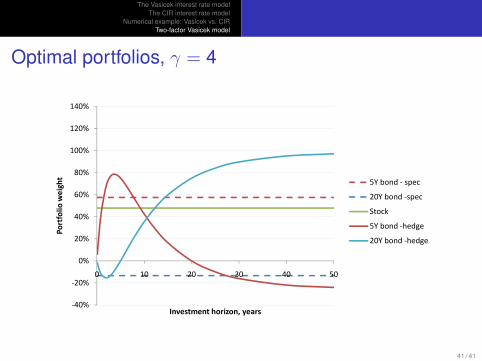
Optimal portfolios, γ = 4
20%
40%
60%
80%
100%
120%
140%
Po
rtfo
lio
we
igh
t
5Y bond - spec
20Y bond -spec
Stock
5Y bond -hedge
20Y bond -hedge
-40%
-20%
0%
20%
40%
60%
80%
100%
120%
140%
0 10 20 30 40 50
Po
rtfo
lio
we
igh
t
Investment horizon, years
5Y bond - spec
20Y bond -spec
Stock
5Y bond -hedge
20Y bond -hedge
41 / 41
Stochastic market price of riskValue/growth tilts and mean reversion
Stochastic volatility
Dynamic Asset AllocationChapter 11: Stochastic market prices of risk
Claus Munk
August 2012
AARHUS UNIVERSITY AU
1 / 49
Stochastic market price of riskValue/growth tilts and mean reversion
Stochastic volatility
Outline
1 Stochastic market price of riskThe basic modelDistribution of future pricesOptimal investment strategy
2 Value/growth tilts and mean reversionThe modelOptimal strategiesSuboptimal strategies
3 Stochastic volatilityModel without hedgingModel with imperfect hedging (incomplete market)Model with perfect hedging (complete market)Other issues
2 / 49
Stochastic market price of riskValue/growth tilts and mean reversion
Stochastic volatility
The basic modelDistribution of future pricesOptimal investment strategy
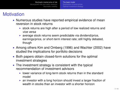
Motivation• Numerous studies have reported empirical evidence of mean
reversion in stock returnsI stock returns are high after a period of low realized returns and
vice versaI average stock returns seem predictable via dividend/price,
earnings/price, or short-term interest rate; still highly debated,though
• Among others Kim and Omberg (1996) and Wachter (2002) havestudied the implications for portfolio decisions
• Both papers obtain closed-form solutions for the optimalinvestment strategies
• The investment strategy is consistent with the typicalrecommendation of investment advisors
I lower variance of long-term stock returns than in the standardmodel
I an investor with a long horizon should invest a larger fraction ofwealth in stocks than an investor with a shorter horizon
5 / 49
Stochastic market price of riskValue/growth tilts and mean reversion
Stochastic volatility
The basic modelDistribution of future pricesOptimal investment strategy
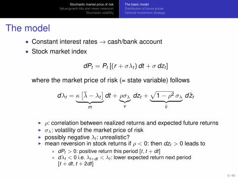
The model• Constant interest rates→ cash/bank account• Stock market index
dPt = Pt [(r + σλt ) dt + σ dzt ]
where the market price of risk (= state variable) follows
dλt = κ[λ− λt
]︸ ︷︷ ︸m
dt + ρσλ︸︷︷︸v
dzt +√
1− ρ2 σλ︸ ︷︷ ︸v
dzt
I ρ: correlation between realized returns and expected future returnsI σλ: volatility of the market price of riskI possibly negative λt : unrealistic?I mean reversion in stock returns if ρ < 0: then dzt > 0 leads to
∗ dPt > 0: positive return this period [t , t + dt]∗ dλt < 0 i.e. λt+dt < λt : lower expected return next period
[t + dt , t + 2dt]
6 / 49
Stochastic market price of riskValue/growth tilts and mean reversion
Stochastic volatility
The basic modelDistribution of future pricesOptimal investment strategy
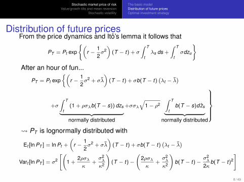
Distribution of future pricesFrom the price dynamics and Ito’s lemma it follows that
PT = Pt exp
{(r −
12σ2)
(T − t) + σ
∫ T
tλs ds +
∫ T
tσdzu
}
After an hour of fun...
PT = Pt exp{(
r −12σ2 + σλ
)(T − t) + σb(T − t)
(λt − λ
)
+σ
∫ T
t(1 + ρσλb(T − s)) dzs︸ ︷︷ ︸normally distributed
+σσλ
√1− ρ2
∫ T
tb(T − s)dzs︸ ︷︷ ︸
normally distributed
PT is lognormally distributed with
Et [ln PT ] = ln Pt +
(r −
12σ2 + σλ
)(T − t) + σb(T − t)
(λt − λ
)Vart [ln PT ] = σ2
[(1 +
2ρσλκ
+σ2λ
κ2
)(T − t)−
(2ρσλκ
+σ2λ
κ2
)b(T − t)−
σ2λ
2κb(T − t)2
]
8 / 49
Stochastic market price of riskValue/growth tilts and mean reversion
Stochastic volatility
The basic modelDistribution of future pricesOptimal investment strategy
Distribution of future prices, cont’d
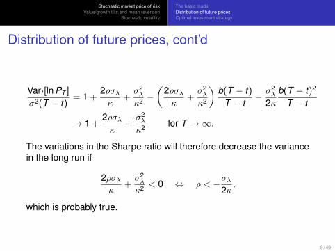
Vart [ln PT ]
σ2(T − t)= 1 +
2ρσλκ
+σ2λ
κ2 −(
2ρσλκ
+σ2λ
κ2
)b(T − t)
T − t− σ2
λ
2κb(T − t)2
T − t
→ 1 +2ρσλκ
+σ2λ
κ2 for T →∞.
The variations in the Sharpe ratio will therefore decrease the variancein the long run if
2ρσλκ
+σ2λ
κ2 < 0 ⇔ ρ < −σλ2κ,
which is probably true.
9 / 49
Stochastic market price of riskValue/growth tilts and mean reversion
Stochastic volatility
The basic modelDistribution of future pricesOptimal investment strategy
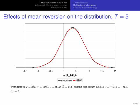
Effects of mean reversion on the distribution, T = 5
-1.5 -1 -0.5 0 0.5 1 1.5 2
ln (P_T/P_0)
mean rev GBM
Parameters: r = 3%, σ = 20%, κ = 0.02, λ = 0.3 (excess exp. return 6%), σλ = 1%, ρ = −0.8,
λt = λ
10 / 49
Stochastic market price of riskValue/growth tilts and mean reversion
Stochastic volatility
The basic modelDistribution of future pricesOptimal investment strategy
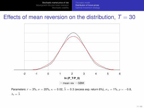
Effects of mean reversion on the distribution, T = 30
-2 -1 0 1 2 3 4 5 6
ln (P_T/P_0)
mean rev GBM
Parameters: r = 3%, σ = 20%, κ = 0.02, λ = 0.3 (excess exp. return 6%), σλ = 1%, ρ = −0.8,
λt = λ
11 / 49
Stochastic market price of riskValue/growth tilts and mean reversion
Stochastic volatility
The basic modelDistribution of future pricesOptimal investment strategy
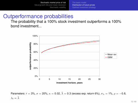
Outperformance probabilitiesThe probability that a 100% stock investment outperforms a 100%bond investment...
0%
20%
40%
60%
80%
100%
0 5 10 15 20 25 30
investment horizon, years
ou
tpe
rfo
rma
nc
e p
rob
ab
ilit
y
Mean rev
GBM
Parameters: r = 3%, σ = 20%, κ = 0.02, λ = 0.3 (excess exp. return 6%), σλ = 1%, ρ = −0.8,
λt = λ12 / 49

Stochastic market price of riskValue/growth tilts and mean reversion
Stochastic volatility
The basic modelDistribution of future pricesOptimal investment strategy
Quadratic modelIt’s a quadratic model with state variable x = λ:• r(x) = r0 + r1x + r2x2: use r0 = r , r1 = r2 = 0• ‖λ(x)‖2 = Λ0 + Λ1x + Λ2x2: use Λ0 = Λ1 = 0,Λ2 = 1• m(x) = m0 + m1x : use m0 = κλ,m1 = −κ• v2 = ρ2σ2
λ is constant• v2 = (1− ρ2)σ2
λ is constant• v(x)λ(x) = K0 + K1x : use K0 = 0,K1 = ρσλ
Plug into general solution from Ch. 7:
A2(τ) =2(
2r2 + Λ2γ
)(eντ − 1)(
ν + 2 γ−1γ
K1 − 2m1
)(eντ − 1) + 2ν
,
A1(τ) =r1 + Λ1
2γ
2r2 + Λ2γ
A2(τ) +4qν
(eντ/2 − 1
)2
(ν + 2 γ−1γ
K1 − 2m1)(eντ − 1) + 2ν,
ν = 2
√(m1 −
γ − 1γ
K1
)2+γ − 1γ
(2r2 +
Λ2
γ
)(‖v‖2 + v2
),
q =
(m0 −
γ − 1γ
K0
)(2r2 +
Λ2
γ
)−(
m1 −γ − 1γ
K1
)(r1 +
Λ1
2γ
).
14 / 49

Stochastic market price of riskValue/growth tilts and mean reversion
Stochastic volatility
The basic modelDistribution of future pricesOptimal investment strategy
Define κ = κ+ γ−1γ ρσλ, assume κ2 + σ2
λ
(ρ2 + γ(1− ρ2)
)γ−1γ2 > 0,
and define ν = 2√κ2 + γ−1
γ2 σ2λ (ρ2 + γ(1− ρ2)).
Then the relevant Ai (τ) functions are
A2(τ) =2γ
eντ − 1(ν + 2κ) (eντ − 1) + 2ν
,
A1(τ) =4κλγν
(eντ/2 − 1
)2
(ν + 2κ) (eντ − 1) + 2ν,
A0(τ) = rτ + κλ
∫ τ
0A1(s) ds +
12σ2λ
∫ τ
0A2(s) ds
− γ − 12γ
σ2λ
(ρ2 + γ(1− ρ2)
) ∫ τ
0A1(s)2 ds
= long and ugly expression
If γ > 1: A1 and A2 positive and increasing
15 / 49
Stochastic market price of riskValue/growth tilts and mean reversion
Stochastic volatility
The basic modelDistribution of future pricesOptimal investment strategy
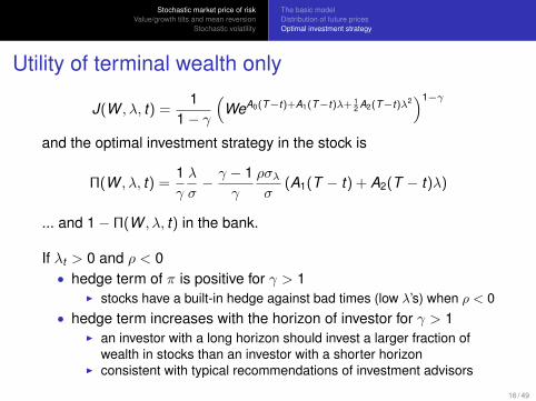
Utility of terminal wealth only
J(W , λ, t) =1
1− γ
(WeA0(T−t)+A1(T−t)λ+ 1
2 A2(T−t)λ2)1−γ
and the optimal investment strategy in the stock is
Π(W , λ, t) =1γ
λ
σ− γ − 1
γ
ρσλσ
(A1(T − t) + A2(T − t)λ)
... and 1− Π(W , λ, t) in the bank.
If λt > 0 and ρ < 0• hedge term of π is positive for γ > 1
I stocks have a built-in hedge against bad times (low λ’s) when ρ < 0• hedge term increases with the horizon of investor for γ > 1
I an investor with a long horizon should invest a larger fraction ofwealth in stocks than an investor with a shorter horizon
I consistent with typical recommendations of investment advisors
16 / 49

Stochastic market price of riskValue/growth tilts and mean reversion
Stochastic volatility
The basic modelDistribution of future pricesOptimal investment strategy
Optimal portfolio weight
70%
75%
80%
85%
90%
0 10 20 30 40 50
investment horizon, years
po
rtfo
lio
we
igh
t
Mean rev
GBM
17 / 49
Stochastic market price of riskValue/growth tilts and mean reversion
Stochastic volatility
The basic modelDistribution of future pricesOptimal investment strategy
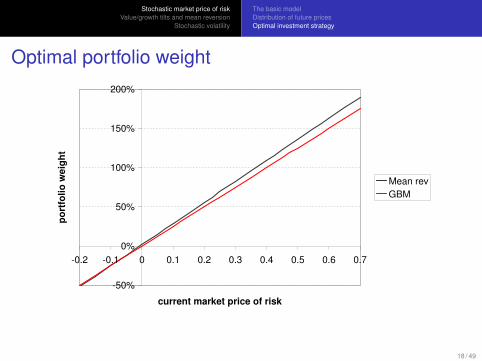
Optimal portfolio weight
-50%
0%
50%
100%
150%
200%
-0.2 -0.1 0 0.1 0.2 0.3 0.4 0.5 0.6 0.7
current market price of risk
po
rtfo
lio
we
igh
t
Mean rev
GBM
18 / 49
Stochastic market price of riskValue/growth tilts and mean reversion
Stochastic volatility
The basic modelDistribution of future pricesOptimal investment strategy
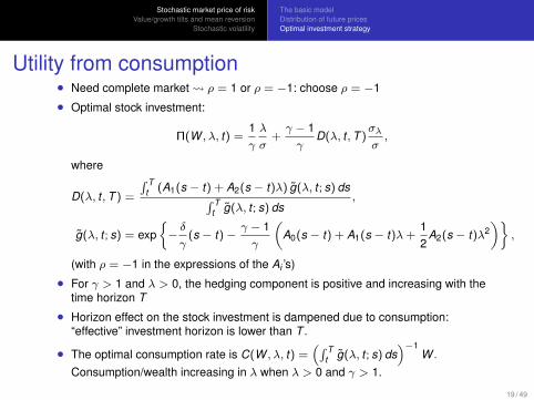
Utility from consumption• Need complete market ρ = 1 or ρ = −1: choose ρ = −1
• Optimal stock investment:
Π(W , λ, t) =1γ
λ
σ+γ − 1γ
D(λ, t ,T )σλ
σ,
where
D(λ, t ,T ) =
∫ Tt (A1(s − t) + A2(s − t)λ) g(λ, t ; s) ds∫ T
t g(λ, t ; s) ds,
g(λ, t ; s) = exp{−δ
γ(s − t)−
γ − 1γ
(A0(s − t) + A1(s − t)λ+
12
A2(s − t)λ2)}
,
(with ρ = −1 in the expressions of the Ai ’s)
• For γ > 1 and λ > 0, the hedging component is positive and increasing with thetime horizon T
• Horizon effect on the stock investment is dampened due to consumption:“effective” investment horizon is lower than T .
• The optimal consumption rate is C(W , λ, t) =(∫ T
t g(λ, t ; s) ds)−1
W .
Consumption/wealth increasing in λ when λ > 0 and γ > 1.
19 / 49
Stochastic market price of riskValue/growth tilts and mean reversion
Stochastic volatility
The modelOptimal strategiesSuboptimal strategies
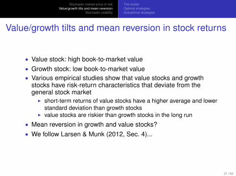
Value/growth tilts and mean reversion in stock returns
• Value stock: high book-to-market value• Growth stock: low book-to-market value• Various empirical studies show that value stocks and growth
stocks have risk-return characteristics that deviate from thegeneral stock market
I short-term returns of value stocks have a higher average and lowerstandard deviation than growth stocks
I value stocks are riskier than growth stocks in the long run
• Mean reversion in growth and value stocks?• We follow Larsen & Munk (2012, Sec. 4)...
21 / 49
Stochastic market price of riskValue/growth tilts and mean reversion
Stochastic volatility
The modelOptimal strategiesSuboptimal strategies
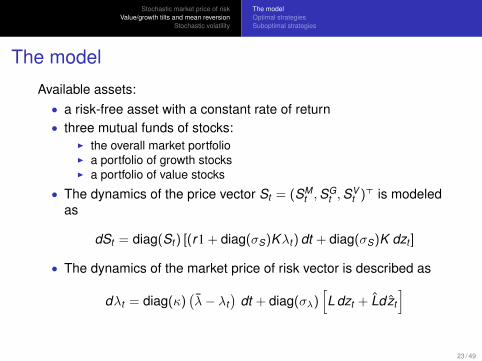
The model
Available assets:• a risk-free asset with a constant rate of return• three mutual funds of stocks:
I the overall market portfolioI a portfolio of growth stocksI a portfolio of value stocks
• The dynamics of the price vector St = (SMt ,S
Gt ,S
Vt )> is modeled
as
dSt = diag(St ) [(r1 + diag(σS)Kλt ) dt + diag(σS)K dzt ]
• The dynamics of the market price of risk vector is described as
dλt = diag(κ)(λ− λt
)dt + diag(σλ)
[L dzt + Ldzt
]
23 / 49
Stochastic market price of riskValue/growth tilts and mean reversion
Stochastic volatility
The modelOptimal strategiesSuboptimal strategies
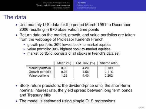
The data• Use monthly U.S. data for the period March 1951 to December
2006 resulting in 670 observation time points• Return data on the market, growth, and value portfolios are taken
from the webpage of Professor Kenenth FrenchI growth portfolio: 30% lowest book-to-market equitiesI value portfolio: 30% highest book-to-market equitiesI market portfolio: consists of all stocks in French’s data set
Mean (%) Std. Dev. (%) Sharpe ratioMarket portfolio 0.99 4.20 0.139Growth portfolio 0.93 4.56 0.116Value portfolio 1.29 4.40 0.202
• Stock return predictors: the dividend-price ratio, the short-termnominal interest rate, the yield spread between long term bondsand Treasury bills
• The model is estimated using simple OLS regressions24 / 49
Stochastic market price of riskValue/growth tilts and mean reversion
Stochastic volatility
The modelOptimal strategiesSuboptimal strategies
Mean reversion in estimated model
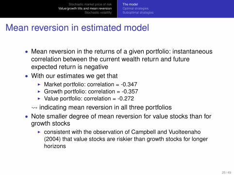
• Mean reversion in the returns of a given portfolio: instantaneouscorrelation between the current wealth return and futureexpected return is negative
• With our estimates we get thatI Market portfolio: correlation = -0.347I Growth portfolio: correlation = -0.357I Value portfolio: correlation = -0.272
indicating mean reversion in all three portfolios• Note smaller degree of mean reversion for value stocks than for
growth stocksI consistent with the observation of Campbell and Vuolteenaho
(2004) that value stocks are riskier than growth stocks for longerhorizons
25 / 49
Stochastic market price of riskValue/growth tilts and mean reversion
Stochastic volatility
The modelOptimal strategiesSuboptimal strategies
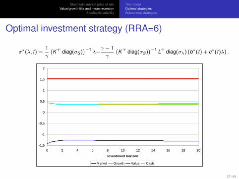
Optimal investment strategy (RRA=6)
π∗(λ, t) =1γ
(K> diag(σS)
)−1λ−
γ − 1γ
(K> diag(σS)
)−1 L> diag(σλ) (b∗(t) + c∗(t)λ) .
-1,5
-1
-0,5
0
0,5
1
1,5
2
0 2 4 6 8 10 12 14 16 18 20
Investment horizon
Market Growth Value Cash
27 / 49
Stochastic market price of riskValue/growth tilts and mean reversion
Stochastic volatility
The modelOptimal strategiesSuboptimal strategies
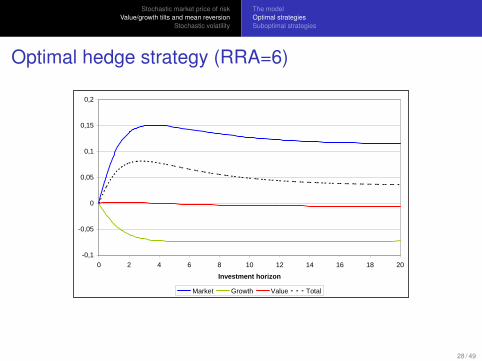
Optimal hedge strategy (RRA=6)
-0,1
-0,05
0
0,05
0,1
0,15
0,2
0 2 4 6 8 10 12 14 16 18 20
Investment horizon
Market Growth Value Total
28 / 49
Stochastic market price of riskValue/growth tilts and mean reversion
Stochastic volatility
The modelOptimal strategiesSuboptimal strategies
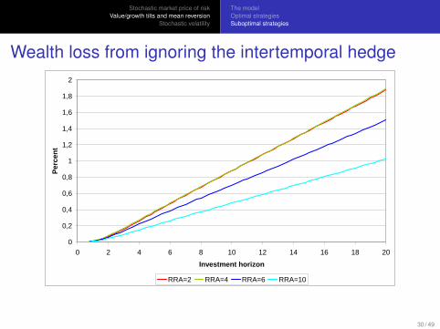
Wealth loss from ignoring the intertemporal hedge
0
0,2
0,4
0,6
0,8
1
1,2
1,4
1,6
1,8
2
0 2 4 6 8 10 12 14 16 18 20
Investment horizon
Per
cen
t
RRA=2 RRA=4 RRA=6 RRA=10
30 / 49
Stochastic market price of riskValue/growth tilts and mean reversion
Stochastic volatility
The modelOptimal strategiesSuboptimal strategies
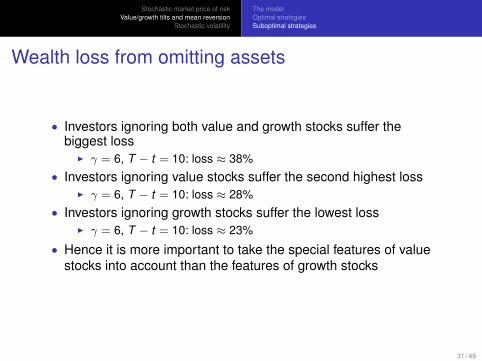
Wealth loss from omitting assets
• Investors ignoring both value and growth stocks suffer thebiggest loss
I γ = 6, T − t = 10: loss ≈ 38%• Investors ignoring value stocks suffer the second highest loss
I γ = 6, T − t = 10: loss ≈ 28%• Investors ignoring growth stocks suffer the lowest loss
I γ = 6, T − t = 10: loss ≈ 23%
• Hence it is more important to take the special features of valuestocks into account than the features of growth stocks
31 / 49
Stochastic market price of riskValue/growth tilts and mean reversion
Stochastic volatility
Model without hedgingModel with imperfect hedging (incomplete market)Model with perfect hedging (complete market)Other issues
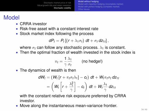
Model• CRRA investor• Risk-free asset with a constant interest rate• Stock market index following the process
dPt = Pt [(r + λ1σt ) dt + σt dz1t ] ,
where σt can follow any stochastic process. λ1 is constant.• Then the optimal fraction of wealth invested in the stock index is
πt =1γ
λ1
σt(no hedge!)
• The dynamics of wealth is then
dWt = (Wt [r + πtσtλ1]− ct ) dt + Wtπtσt dz1t
=
(Wt
[r +
λ21γ
]− ct
)dt + Wt
λ1
γdz1t
with the constant relative risk exposure preferred by CRRAinvestor.
• Move along the instantaneous mean-variance frontier.34 / 49
Stochastic market price of riskValue/growth tilts and mean reversion
Stochastic volatility
Model without hedgingModel with imperfect hedging (incomplete market)Model with perfect hedging (complete market)Other issues
Heston-type model, no options
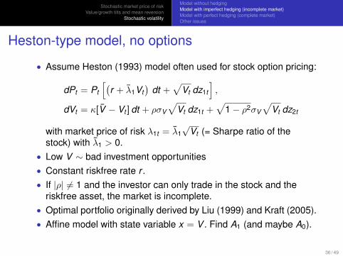
• Assume Heston (1993) model often used for stock option pricing:
dPt = Pt
[(r + λ1Vt
)dt +
√Vt dz1t
],
dVt = κ[V − Vt ] dt + ρσV
√Vt dz1t +
√1− ρ2σV
√Vt dz2t
with market price of risk λ1t = λ1√
Vt (= Sharpe ratio of thestock) with λ1 > 0.
• Low V ∼ bad investment opportunities• Constant riskfree rate r .• If |ρ| 6= 1 and the investor can only trade in the stock and the
riskfree asset, the market is incomplete.• Optimal portfolio originally derived by Liu (1999) and Kraft (2005).• Affine model with state variable x = V . Find A1 (and maybe A0).
36 / 49

Stochastic market price of riskValue/growth tilts and mean reversion
Stochastic volatility
Model without hedgingModel with imperfect hedging (incomplete market)Model with perfect hedging (complete market)Other issues
Heston-type model, no options – cont’dIn general affine model:
r(x) = r0 + r1x , m(x) = m0 + m1x ,
v(x)2 = v0 + v1x , ‖v(x)‖2 = V0 + V1x ,
‖λ(x)‖2 = Λ0 + Λ1x , v(x)>λ(x) = K0 + K1x
A1(τ) =2(
r1 + Λ12γ
)(eντ − 1)(
ν + γ−1γ
K1 −m1
)(eντ − 1) + 2ν
,
ν =
√(m1 −
γ − 1γ
K1
)2
+ 2γ − 1γ
(r1 +
Λ1
2γ
)(V1 + γv1)
Assume γ > 1 and define
κ = κ+γ − 1γ
ρσV λ1, ν =
√κ2 +
γ − 1γ2 λ2
1σ2V (ρ2 + γ[1− ρ2])
Then A1(τ) =λ2
1γ
eντ−1(ν+κ)(eντ−1)+2ν .
37 / 49
Stochastic market price of riskValue/growth tilts and mean reversion
Stochastic volatility
Model without hedgingModel with imperfect hedging (incomplete market)Model with perfect hedging (complete market)Other issues
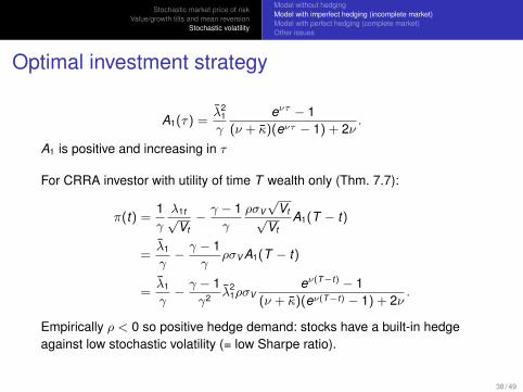
Optimal investment strategy
A1(τ) =λ2
1
γ
eντ − 1(ν + κ)(eντ − 1) + 2ν
.
A1 is positive and increasing in τ
For CRRA investor with utility of time T wealth only (Thm. 7.7):
π(t) =1γ
λ1t√Vt− γ − 1
γ
ρσV√
Vt√Vt
A1(T − t)
=λ1
γ− γ − 1
γρσV A1(T − t)
=λ1
γ− γ − 1
γ2 λ21ρσV
eν(T−t) − 1(ν + κ)(eν(T−t) − 1) + 2ν
.
Empirically ρ < 0 so positive hedge demand: stocks have a built-in hedgeagainst low stochastic volatility (= low Sharpe ratio).
38 / 49
Stochastic market price of riskValue/growth tilts and mean reversion
Stochastic volatility
Model without hedgingModel with imperfect hedging (incomplete market)Model with perfect hedging (complete market)Other issues
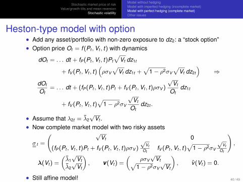
Heston-type model with option• Add any asset/portfolio with non-zero exposure to dz2: a “stock option”• Option price Ot = f (Pt ,Vt , t) with dynamics
dOt = . . . dt + fP(Pt ,Vt , t)Pt
√Vt dz1t
+ fV (Pt ,Vt , t)(ρσV
√Vt dz1t +
√1− ρ2σV
√Vt dz2t
)⇒
dOt
Ot= . . . dt + (fP(Pt ,Vt , t)Pt + fV (Pt ,Vt , t)ρσV )
√Vt
Otdz1t
+ fV (Pt ,Vt , t)√
1− ρ2σV
√Vt
Otdz2t .
• Assume that λ2t = λ2√
Vt .• Now complete market model with two risky assets
σ t =
( √Vt 0
(fP(Pt ,Vt , t)Pt + fV (Pt ,Vt , t)ρσV )
√Vt
OtfV (Pt ,Vt , t)
√1− ρ2σV
√Vt
Ot
),
λ(Vt ) =
(λ1√
Vt
λ2√
Vt
), v(Vt ) =
(ρσV√
Vt√1− ρ2σV
√Vt
), v(Vt ) = 0.
• Still affine model! 40 / 49
Stochastic market price of riskValue/growth tilts and mean reversion
Stochastic volatility
Model without hedgingModel with imperfect hedging (incomplete market)Model with perfect hedging (complete market)Other issues
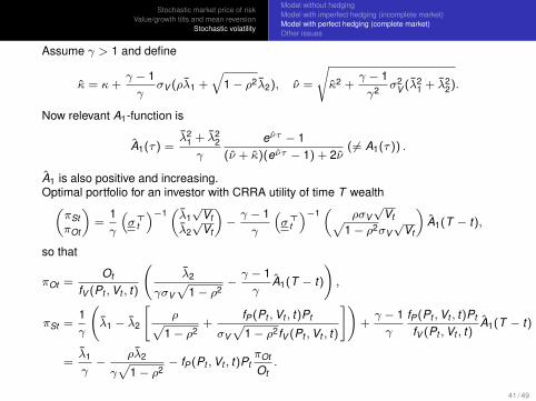
Assume γ > 1 and define
κ = κ+γ − 1γ
σV (ρλ1 +√
1− ρ2λ2), ν =
√κ2 +
γ − 1γ2
σ2V (λ2
1 + λ22).
Now relevant A1-function is
A1(τ) =λ2
1 + λ22
γ
eντ − 1(ν + κ)(eντ − 1) + 2ν
( 6= A1(τ)) .
A1 is also positive and increasing.Optimal portfolio for an investor with CRRA utility of time T wealth(
πStπOt
)=
1γ
(σ>
t
)−1(λ1√
Vtλ2√
Vt
)−γ − 1γ
(σ>
t
)−1(
ρσV√
Vt√1− ρ2σV
√Vt
)A1(T − t),
so that
πOt =Ot
fV (Pt ,Vt , t)
(λ2
γσV√
1− ρ2−γ − 1γ
A1(T − t)
),
πSt =1γ
(λ1 − λ2
[ρ√
1− ρ2+
fP(Pt ,Vt , t)Pt
σV√
1− ρ2fV (Pt ,Vt , t)
])+γ − 1γ
fP(Pt ,Vt , t)Pt
fV (Pt ,Vt , t)A1(T − t)
=λ1
γ−
ρλ2
γ√
1− ρ2− fP(Pt ,Vt , t)Pt
πOt
Ot.
41 / 49
Stochastic market price of riskValue/growth tilts and mean reversion
Stochastic volatility
Model without hedgingModel with imperfect hedging (incomplete market)Model with perfect hedging (complete market)Other issues
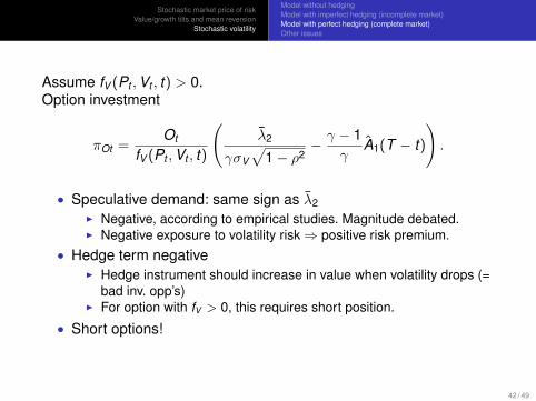
Assume fV (Pt ,Vt , t) > 0.Option investment
πOt =Ot
fV (Pt ,Vt , t)
(λ2
γσV√
1− ρ2− γ − 1
γA1(T − t)
).
• Speculative demand: same sign as λ2I Negative, according to empirical studies. Magnitude debated.I Negative exposure to volatility risk⇒ positive risk premium.
• Hedge term negativeI Hedge instrument should increase in value when volatility drops (=
bad inv. opp’s)I For option with fV > 0, this requires short position.
• Short options!
42 / 49
Stochastic market price of riskValue/growth tilts and mean reversion
Stochastic volatility
Model without hedgingModel with imperfect hedging (incomplete market)Model with perfect hedging (complete market)Other issues
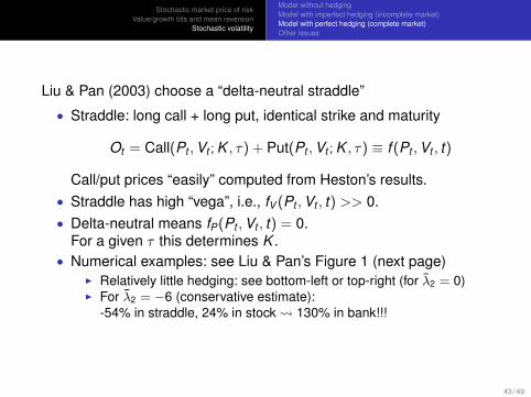
Liu & Pan (2003) choose a “delta-neutral straddle”
• Straddle: long call + long put, identical strike and maturity
Ot = Call(Pt ,Vt ; K , τ) + Put(Pt ,Vt ; K , τ) ≡ f (Pt ,Vt , t)
Call/put prices “easily” computed from Heston’s results.• Straddle has high “vega”, i.e., fV (Pt ,Vt , t) >> 0.• Delta-neutral means fP(Pt ,Vt , t) = 0.
For a given τ this determines K .• Numerical examples: see Liu & Pan’s Figure 1 (next page)
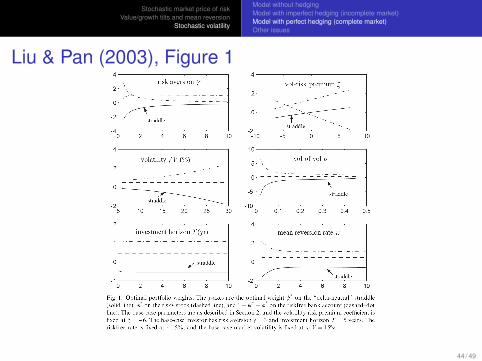
I Relatively little hedging: see bottom-left or top-right (for λ2 = 0)I For λ2 = −6 (conservative estimate):
-54% in straddle, 24% in stock 130% in bank!!!
43 / 49
Stochastic market price of riskValue/growth tilts and mean reversion
Stochastic volatility
Model without hedgingModel with imperfect hedging (incomplete market)Model with perfect hedging (complete market)Other issues
Liu & Pan (2003), Figure 1
44 / 49
Stochastic market price of riskValue/growth tilts and mean reversion
Stochastic volatility
Model without hedgingModel with imperfect hedging (incomplete market)Model with perfect hedging (complete market)Other issues
Losses from suboptimal strategies
See Liu & Pan (2003) and Larsen & Munk (2012)
• Important to include options in the speculative portfolio becauseof the apparently very attractive risk-return tradeoff
I highly depending on the estimate of λ2!• Relatively little is gained by the intertemporal hedge
I highly depending on the functional form assumed for the marketprices of risk
45 / 49
Stochastic market price of riskValue/growth tilts and mean reversion
Stochastic volatility
Model without hedgingModel with imperfect hedging (incomplete market)Model with perfect hedging (complete market)Other issues
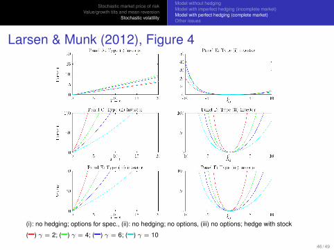
Larsen & Munk (2012), Figure 4
(i): no hedging; options for spec., (ii): no hedging; no options, (iii) no options; hedge with stock
(–) γ = 2; (–) γ = 4; (–) γ = 6; (–) γ = 10
46 / 49
Stochastic market price of riskValue/growth tilts and mean reversion
Stochastic volatility
Model without hedgingModel with imperfect hedging (incomplete market)Model with perfect hedging (complete market)Other issues
Jumps
• Liu & Pan allow for jumps of given size (large negative, “crash”)I Jump arrival intensity proportional to VtI Need estimate of jump risk premium (high?)I Need another jump-sensitive option to complete the market, e.g.,
an out-of-the-money putI Affine jump-diffusion type model closed-form solutionI Their Table 1 shows that the optimal put position is very sensitive to
assumed jump parameters
• Jumps of many possible sizes need more options to completethe market
• Jumps in volatility?Liu, Longstaff & Pan (2003), Branger, Schlag & Schneider (2008)
• Need to learn more about theoretical asset pricing withstochastic volatility and jumps to understand the relevant marketprices of risk!
48 / 49
Stochastic market price of riskValue/growth tilts and mean reversion
Stochastic volatility
Model without hedgingModel with imperfect hedging (incomplete market)Model with perfect hedging (complete market)Other issues
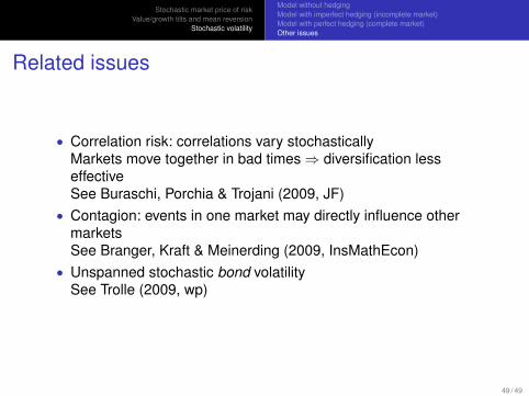
Related issues
• Correlation risk: correlations vary stochasticallyMarkets move together in bad times⇒ diversification lesseffectiveSee Buraschi, Porchia & Trojani (2009, JF)
• Contagion: events in one market may directly influence othermarketsSee Branger, Kraft & Meinerding (2009, InsMathEcon)
• Unspanned stochastic bond volatilitySee Trolle (2009, wp)
49 / 49
IntroductionMerton with income
Constraints and better income modelInterest rate risk and labor income
Dynamic Asset AllocationChapter 13: Labor income
Claus Munk
August 2012
AARHUS UNIVERSITY AU
1 / 73
IntroductionMerton with income
Constraints and better income modelInterest rate risk and labor income
Outline
1 Introduction
2 Merton with income
3 Constraints and better income model
4 Interest rate risk and labor income
2 / 73
IntroductionMerton with income
Constraints and better income modelInterest rate risk and labor income
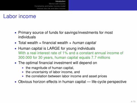
Labor income
• Primary source of funds for savings/investments for mostindividuals
• Total wealth = financial wealth + human capital• Human capital is LARGE for young individuals
With a real interest rate of 1% and a constant annual income of300.000 for 30 years, human capital equals 7.7 millions
• The optimal financial investment will depend onI the magnitude of human capital,I the uncertainty of labor income, andI the correlation between labor income and asset prices
• Obvious horizon effects in human capital — life-cycle perspective
4 / 73
IntroductionMerton with income
Constraints and better income modelInterest rate risk and labor income
Modeling issues
• exogenous or endogenous income ( labor supply decision)• correlations with asset returns; spanned or unspanned income• variations in labor income over the life-cycle• variations in labor income over the business cycle• restrictions on borrowing with future income as implicit collateral
(moral hazard, adverse selection)• disability risk, unemployment risk, mortality risk
5 / 73
IntroductionMerton with income
Constraints and better income modelInterest rate risk and labor income
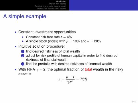
A simple example
• Constant investment opportunitiesI Constant risk-free rate r = 4%I A single stock (index) with µ = 10% and σ = 20%
• Intuitive solution procedure:1 find desired riskiness of total wealth2 adjust for risk profile of human capital in order to find desired
riskiness of financial wealth3 find the portfolio with desired riskiness of financial wealth
• With RRA γ = 2, the optimal fraction of total wealth in the riskyasset is
π =µ− rγσ2 = 75%
6 / 73
IntroductionMerton with income
Constraints and better income modelInterest rate risk and labor income
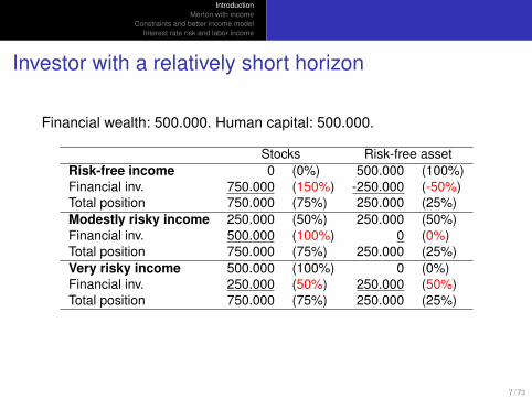
Investor with a relatively short horizon
Financial wealth: 500.000. Human capital: 500.000.
Stocks Risk-free assetRisk-free income 0 (0%) 500.000 (100%)Financial inv. 750.000 (150%) -250.000 (-50%)Total position 750.000 (75%) 250.000 (25%)Modestly risky income 250.000 (50%) 250.000 (50%)Financial inv. 500.000 (100%) 0 (0%)Total position 750.000 (75%) 250.000 (25%)Very risky income 500.000 (100%) 0 (0%)Financial inv. 250.000 (50%) 250.000 (50%)Total position 750.000 (75%) 250.000 (25%)
7 / 73
IntroductionMerton with income
Constraints and better income modelInterest rate risk and labor income
Investor with a relatively long horizon
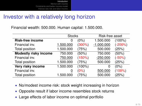
Financial wealth: 500.000. Human capital: 1.500.000.
Stocks Risk-free assetRisk-free income 0 (0%) 1.500.000 (100%)Financial inv. 1.500.000 (300%) -1.000.000 (-200%)Total position 1.500.000 (75%) 500.000 (25%)Modestly risky income 750.000 (50%) 750.000 (50%)Financial inv. 750.000 (150%) -250.000 (-50%)Total position 1.500.000 (75%) 500.000 (25%)Very risky income 1.500.000 (100%) 0 (0%)Financial inv. 0 (0%) 500.000 (100%)Total position 1.500.000 (75%) 500.000 (25%)
• No/modest income risk: stock weight increasing in horizon• Opposite result if labor income resembles stock returns• Large effects of labor income on optimal portfolio
8 / 73
IntroductionMerton with income
Constraints and better income modelInterest rate risk and labor income
Exogenous incomeEndogenous income
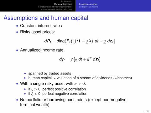
Assumptions and human capital• Constant interest rate r• Risky asset prices:
dP t = diag(P t )[(
r1 + σλ)
dt + σ dz t]
• Annualized income rate:
dyt = yt [α dt + ξ> dz t ]
I spanned by traded assetsI human capital ∼ valuation of a stream of dividends (=incomes)
• With a single risky asset with σ > 0:I if ξ > 0: perfect positive correlationI if ξ < 0: perfect negative correlation
• No portfolio or borrowing constraints (except non-negativeterminal wealth)
11 / 73
IntroductionMerton with income
Constraints and better income modelInterest rate risk and labor income
Exogenous incomeEndogenous income
Human capital with spanned income
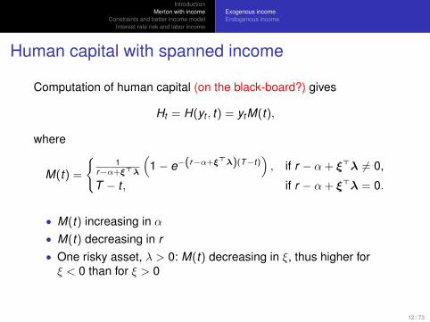
Computation of human capital (on the black-board?) gives
Ht = H(yt , t) = ytM(t),
where
M(t) =
{1
r−α+ξ>λ
(1− e−(r−α+ξ>λ)(T−t)
), if r − α + ξ>λ 6= 0,
T − t , if r − α + ξ>λ = 0.
• M(t) increasing in α• M(t) decreasing in r• One risky asset, λ > 0: M(t) decreasing in ξ, thus higher forξ < 0 than for ξ > 0
12 / 73
IntroductionMerton with income
Constraints and better income modelInterest rate risk and labor income
Exogenous incomeEndogenous income
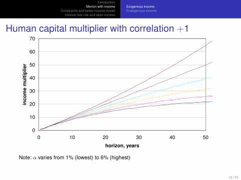
Human capital multiplier with correlation +1
0
10
20
30
40
50
60
70
0 10 20 30 40 50
horizon, years
inco
me m
ult
ipli
er
Note: α varies from 1% (lowest) to 6% (highest)
13 / 73
IntroductionMerton with income
Constraints and better income modelInterest rate risk and labor income
Exogenous incomeEndogenous income
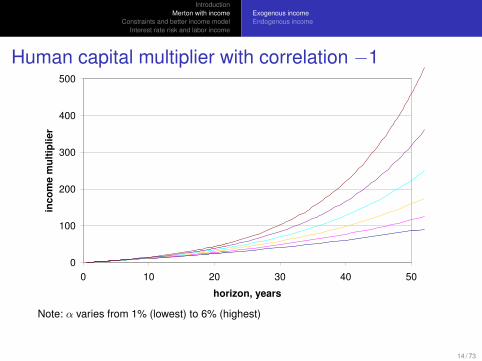
Human capital multiplier with correlation −1
0
100
200
300
400
500
0 10 20 30 40 50
horizon, years
inco
me m
ult
ipli
er
Note: α varies from 1% (lowest) to 6% (highest)
14 / 73

IntroductionMerton with income
Constraints and better income modelInterest rate risk and labor income
Exogenous incomeEndogenous income
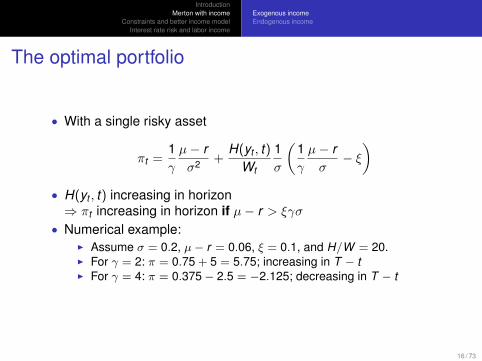
The optimal portfolio
• Intuitive derivation: on the black-board?• Formal derivation: solve HJB-equation• Optimal amounts:
θt =1γ
(Wt + H(yt , t))(σ>)−1
λ− H(yt , t)(σ>)−1
ξ
• Portfolio weights:
πt =1γ
(σ>)−1
λ +H(yt , t)
W(σ>)−1
(1γλ− ξ
)
15 / 73
IntroductionMerton with income
Constraints and better income modelInterest rate risk and labor income
Exogenous incomeEndogenous income
The optimal portfolio
• With a single risky asset
πt =1γ
µ− rσ2 +
H(yt , t)Wt
1σ
(1γ
µ− rσ− ξ)
• H(yt , t) increasing in horizon⇒ πt increasing in horizon if µ− r > ξγσ
• Numerical example:I Assume σ = 0.2, µ− r = 0.06, ξ = 0.1, and H/W = 20.I For γ = 2: π = 0.75 + 5 = 5.75; increasing in T − tI For γ = 4: π = 0.375− 2.5 = −2.125; decreasing in T − t
16 / 73
IntroductionMerton with income
Constraints and better income modelInterest rate risk and labor income
Exogenous incomeEndogenous income
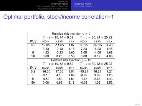
Optimal portfolio, stock/income correlation=1
Relative risk aversion γ = 2T − t = 10, M = 9.52 T − t = 30, M = 25.92
W/y stock cash c/y stock cash c/y0.2 12.65 -11.65 1.07 33.15 -32.15 1.401 3.13 -2.13 1.16 7.23 -6.23 1.455 1.23 -0.23 1.60 2.05 -1.05 1.66
50 0.80 0.20 6.55 0.88 0.12 4.08Relative risk aversion γ = 10
T − t = 10, M = 9.52 T − t = 30, M = 25.92W/y stock cash c/y stock cash c/y0.2 -16.50 17.50 1.01 -45.21 46.21 1.211 -3.18 4.18 1.09 -8.92 9.92 1.255 -0.52 1.52 1.51 -1.66 2.66 1.43
50 0.08 0.92 6.18 -0.03 1.03 3.52
17 / 73
IntroductionMerton with income
Constraints and better income modelInterest rate risk and labor income
Exogenous incomeEndogenous income
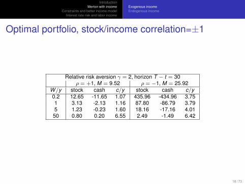
Optimal portfolio, stock/income correlation=±1
Relative risk aversion γ = 2, horizon T − t = 30ρ = +1, M = 9.52 ρ = −1, M = 25.92
W/y stock cash c/y stock cash c/y0.2 12.65 -11.65 1.07 435.96 -434.96 3.751 3.13 -2.13 1.16 87.80 -86.79 3.795 1.23 -0.23 1.60 18.16 -17.16 4.01
50 0.80 0.20 6.55 2.49 -1.49 6.42
18 / 73
IntroductionMerton with income
Constraints and better income modelInterest rate risk and labor income
Exogenous incomeEndogenous income
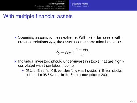
With multiple financial assets
• Spanning assumption less extreme. With n similar assets withcross-correlations ρPP , the asset-income correlation has to be
ρ2Py = ρPP +
1− ρPP
n.
• Individual investors should under-invest in stocks that are highlycorrelated with their labor income
I 58% of Enron’s 401k pension fund was invested in Enron stocksprior to the 98.8% drop in the Enron stock price in 2001
19 / 73
IntroductionMerton with income
Constraints and better income modelInterest rate risk and labor income
Exogenous incomeEndogenous income
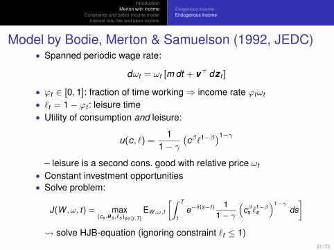
Model by Bodie, Merton & Samuelson (1992, JEDC)• Spanned periodic wage rate:
dωt = ωt [m dt + v> dz t ]
• ϕt ∈ [0,1]: fraction of time working⇒ income rate ϕtωt
• `t = 1− ϕt : leisure time• Utility of consumption and leisure:
u(c, `) =1
1− γ(cβ`1−β)1−γ
– leisure is a second cons. good with relative price ωt
• Constant investment opportunities• Solve problem:
J(W , ω, t) = max(cs,θs,`s)s∈[t,T ]
EW ,ω,t
[∫ T
te−δ(s−t) 1
1− γ
(cβs `
1−βs
)1−γds]
solve HJB-equation (ignoring constraint `t ≤ 1)21 / 73
IntroductionMerton with income
Constraints and better income modelInterest rate risk and labor income
Exogenous incomeEndogenous income
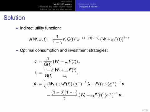
Solution
• Indirect utility function:
J(W , ω, t) =1
1− γK G(t)γω−(1−β)(1−γ) (W + ωF (t))1−γ
• Optimal consumption and investment strategies:
ct =β
G(t)(Wt + ωtF (t)) ,
`t =1− βG(t)
Wt + ωtF (t)ωt
,
θt =1γ
(Wt + ωtF (t))(σ>)−1
λ− F (t)ωt(σ>)−1 v
− (1− β)(1− γ)
γ(Wt + ωtF (t))
(σ>)−1 v .
22 / 73
IntroductionMerton with income
Constraints and better income modelInterest rate risk and labor income
Exogenous incomeEndogenous income
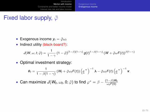
Fixed labor supply, ϕ
• Exogenous income yt = ϕωt
• Indirect utility (black-board?):
J(W , ω, t ; ϕ) =1
1 − γ(1 − ϕ)(1−β)(1−γ) g(t)1−β(1−γ) (W + ϕωF (t))β(1−γ)
• Optimal investment strategy:
θt =1
1 − β(1 − γ)(Wt + ϕωt F (t))
(σ>)−1
λ− ϕωt F (t)(σ>)−1
v .
• Can maximize J(W0, ω0,0; ϕ) to find ϕ∗ = β − (1−β)W0ω0F (0)
23 / 73

IntroductionMerton with income
Constraints and better income modelInterest rate risk and labor income
Exogenous incomeEndogenous income
Labor supply flexibility and optimal risk-taking• Assume a single risky asset and a deterministic wage rate• Optimal investment with flexible labor supply:
θflext =
1γ
(Wt + ωtF (t))λ
σ
• Optimal investment with fixed labor supply:
θfixt =
11− β(1− γ)
(Wt + ϕωtF (t))λ
σ
• If γ < 1, then θflext > θfix
t
• “Take more risk when you can adjust labor supply”• Intuition: compensate for bad returns by working harder• Same conclusion for γ “somewhat higher than” 1, in particular
when ωF (t)/W is high (young investors)• Conclusions unclear with risky (maybe unspanned) wage
24 / 73
IntroductionMerton with income
Constraints and better income modelInterest rate risk and labor income
Models should be improvedThe Cocco-Gomes-Maenhout paper
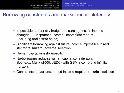
Borrowing constraints and market incompleteness
• Impossible to perfectly hedge or insure against all incomechanges — unspanned income; incomplete market(including real estate helps)
• Significant borrowing against future income impossible in reallife: moral hazard, adverse selection
• Human capital investor-specific• No-borrowing reduces human capital considerably.
See, e.g., Munk (2000, JEDC) with GBM income and infinitehorizon.
• Constraints and/or unspanned income require numerical solution
27 / 73
IntroductionMerton with income
Constraints and better income modelInterest rate risk and labor income
Models should be improvedThe Cocco-Gomes-Maenhout paper
Income variations over life cycle and business cycle
• Life cycle [discrete time]:Cocco, Gomes & Maenhout, “Consumption and Portfolio Choiceover the Life Cycle”, Review of Financial Studies, 2005.
• Life and business cycle [interest rates, cont. time]:Munk & Sørensen, “Dynamic Asset Allocation with StochasticIncome and Interest Rates”, Journal of Financial Economics,2010.
• Life and business cycle [dividend yield, discrete time]:Lynch & Tan, “Labor Income Dynamics at Business-CycleFrequencies”, Journal of Financial Economics, forthcoming.
28 / 73
IntroductionMerton with income
Constraints and better income modelInterest rate risk and labor income
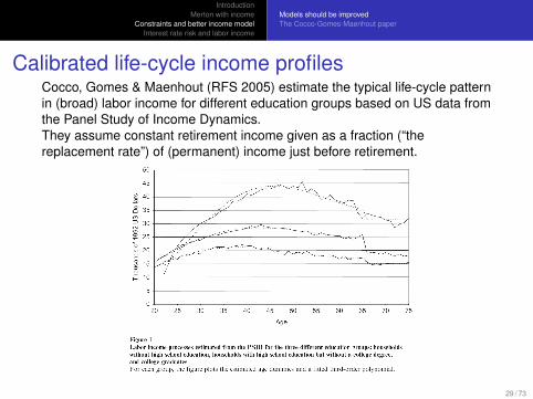
Models should be improvedThe Cocco-Gomes-Maenhout paper
Calibrated life-cycle income profilesCocco, Gomes & Maenhout (RFS 2005) estimate the typical life-cycle patternin (broad) labor income for different education groups based on US data fromthe Panel Study of Income Dynamics.They assume constant retirement income given as a fraction (“thereplacement rate”) of (permanent) income just before retirement.
29 / 73
IntroductionMerton with income
Constraints and better income modelInterest rate risk and labor income
Models should be improvedThe Cocco-Gomes-Maenhout paper
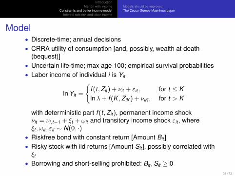
Model• Discrete-time; annual decisions• CRRA utility of consumption [and, possibly, wealth at death
(bequest)]• Uncertain life-time; max age 100; empirical survival probabilities• Labor income of individual i is Yit
ln Yit =
{f (t ,Zit ) + νit + εit , for t ≤ Klnλ+ f (K ,ZiK ) + νiK , for t > K
with deterministic part f (t ,Zit ), permanent income shockνit = νi,t−1 + ξt + ωit and transitory income shock εit , whereξt , ωit , εit ∼ N(0, ·)
• Riskfree bond with constant return [Amount Bit ]• Risky stock with iid returns [Amount Sit ], possibly correlated withξt
• Borrowing and short-selling prohibited: Bit ,Sit ≥ 031 / 73
IntroductionMerton with income
Constraints and better income modelInterest rate risk and labor income
Models should be improvedThe Cocco-Gomes-Maenhout paper
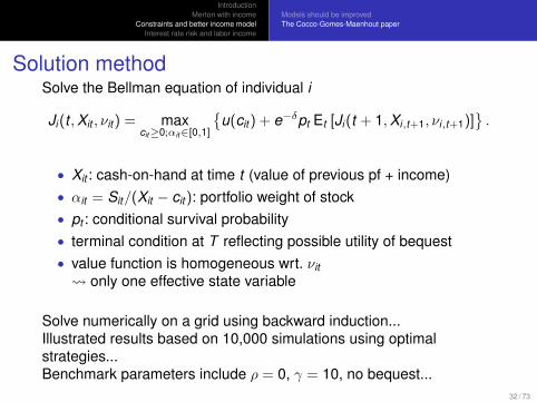
Solution methodSolve the Bellman equation of individual i
Ji (t ,Xit , νit ) = maxcit≥0;αit∈[0,1]
{u(cit ) + e−δpt Et [Ji (t + 1,Xi,t+1, νi,t+1)]
}.
• Xit : cash-on-hand at time t (value of previous pf + income)• αit = Sit/(Xit − cit ): portfolio weight of stock• pt : conditional survival probability• terminal condition at T reflecting possible utility of bequest• value function is homogeneous wrt. νit only one effective state variable
Solve numerically on a grid using backward induction...Illustrated results based on 10,000 simulations using optimalstrategies...Benchmark parameters include ρ = 0, γ = 10, no bequest...
32 / 73
IntroductionMerton with income
Constraints and better income modelInterest rate risk and labor income
Models should be improvedThe Cocco-Gomes-Maenhout paper
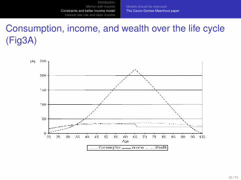
Consumption, income, and wealth over the life cycle(Fig3A)
33 / 73
IntroductionMerton with income
Constraints and better income modelInterest rate risk and labor income
Models should be improvedThe Cocco-Gomes-Maenhout paper
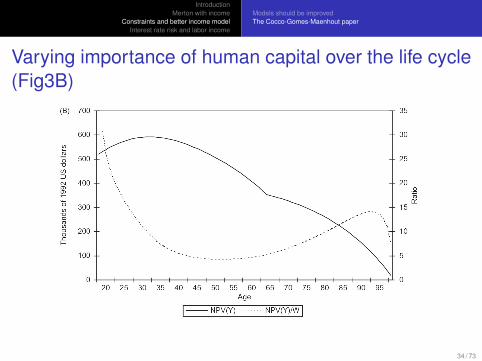
Varying importance of human capital over the life cycle(Fig3B)
34 / 73
IntroductionMerton with income
Constraints and better income modelInterest rate risk and labor income
Models should be improvedThe Cocco-Gomes-Maenhout paper
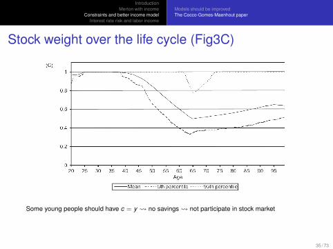
Stock weight over the life cycle (Fig3C)
Some young people should have c = y no savings not participate in stock market
35 / 73
IntroductionMerton with income
Constraints and better income modelInterest rate risk and labor income
Models should be improvedThe Cocco-Gomes-Maenhout paper
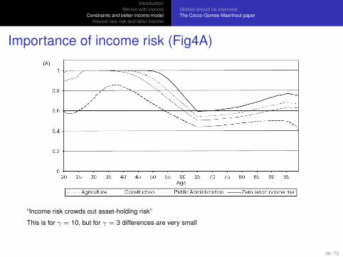
Importance of income risk (Fig4A)
“Income risk crowds out asset-holding risk”
This is for γ = 10, but for γ = 3 differences are very small
36 / 73
IntroductionMerton with income
Constraints and better income modelInterest rate risk and labor income
Models should be improvedThe Cocco-Gomes-Maenhout paper
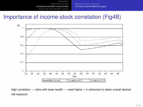
Importance of income-stock correlation (Fig4B)
High correlation retire with lower wealth need higher π in retirement to obtain overall desired
risk exposure
37 / 73
IntroductionMerton with income
Constraints and better income modelInterest rate risk and labor income
Models should be improvedThe Cocco-Gomes-Maenhout paper
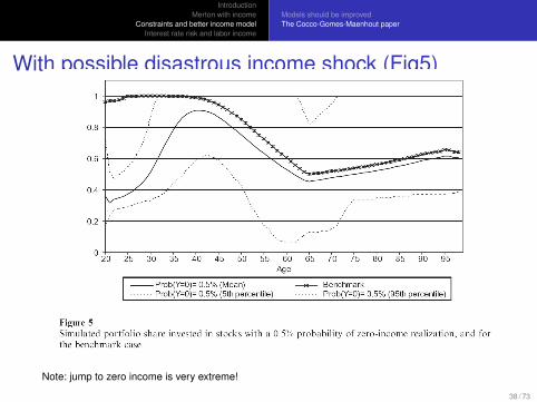
With possible disastrous income shock (Fig5)
Note: jump to zero income is very extreme!
38 / 73
IntroductionMerton with income
Constraints and better income modelInterest rate risk and labor income
Models should be improvedThe Cocco-Gomes-Maenhout paper
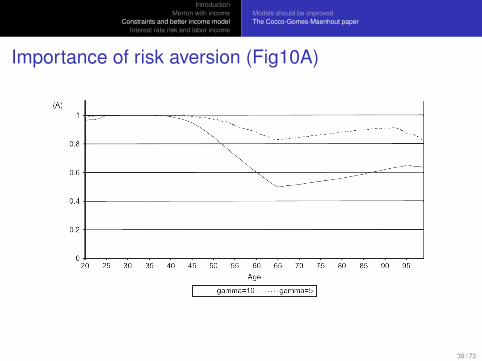
Importance of risk aversion (Fig10A)
39 / 73
IntroductionMerton with income
Constraints and better income modelInterest rate risk and labor income
Models should be improvedThe Cocco-Gomes-Maenhout paper
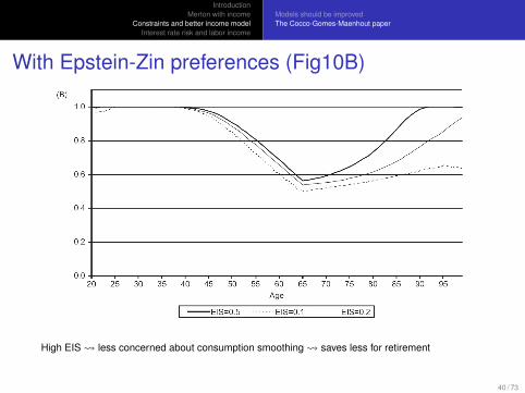
With Epstein-Zin preferences (Fig10B)
High EIS less concerned about consumption smoothing saves less for retirement
40 / 73
IntroductionMerton with income
Constraints and better income modelInterest rate risk and labor income
ModelSpanned income and no portfolio constraintsUnspanned income and portfolio constraintsEmpirical life-cycle variations in income
Labor income and interest rate uncertainty
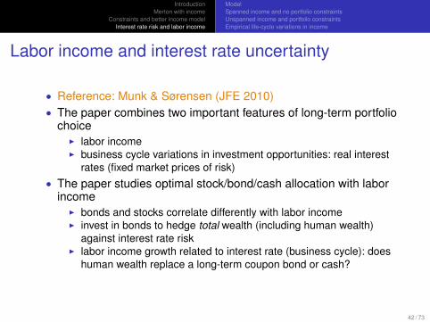
• Reference: Munk & Sørensen (JFE 2010)• The paper combines two important features of long-term portfolio
choiceI labor incomeI business cycle variations in investment opportunities: real interest
rates (fixed market prices of risk)• The paper studies optimal stock/bond/cash allocation with labor
incomeI bonds and stocks correlate differently with labor incomeI invest in bonds to hedge total wealth (including human wealth)
against interest rate riskI labor income growth related to interest rate (business cycle): does
human wealth replace a long-term coupon bond or cash?
42 / 73
IntroductionMerton with income
Constraints and better income modelInterest rate risk and labor income
ModelSpanned income and no portfolio constraintsUnspanned income and portfolio constraintsEmpirical life-cycle variations in income
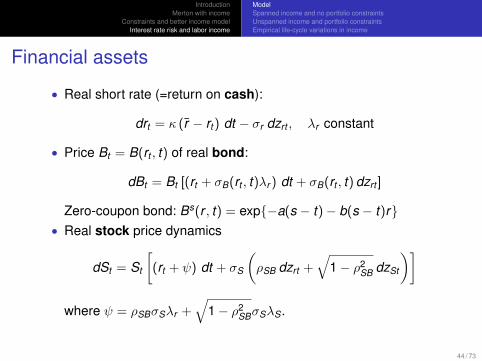
Financial assets
• Real short rate (=return on cash):
drt = κ (r − rt ) dt − σr dzrt , λr constant
• Price Bt = B(rt , t) of real bond:
dBt = Bt [(rt + σB(rt , t)λr ) dt + σB(rt , t) dzrt ]
Zero-coupon bond: Bs(r , t) = exp{−a(s − t)− b(s − t)r}• Real stock price dynamics
dSt = St
[(rt + ψ) dt + σS
(ρSB dzrt +
√1− ρ2
SB dzSt
)]
where ψ = ρSBσSλr +√
1− ρ2SBσSλS.
44 / 73
IntroductionMerton with income
Constraints and better income modelInterest rate risk and labor income
ModelSpanned income and no portfolio constraintsUnspanned income and portfolio constraintsEmpirical life-cycle variations in income
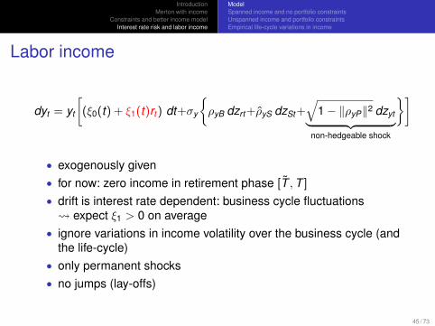
Labor income
dyt = yt
[(ξ0(t) + ξ1(t)rt ) dt+σy
{ρyB dzrt +ρyS dzSt +
√1− ‖ρyP‖2 dzyt︸ ︷︷ ︸
non-hedgeable shock
}]
• exogenously given• for now: zero income in retirement phase [T ,T ]
• drift is interest rate dependent: business cycle fluctuations expect ξ1 > 0 on average
• ignore variations in income volatility over the business cycle (andthe life-cycle)
• only permanent shocks• no jumps (lay-offs)
45 / 73
IntroductionMerton with income
Constraints and better income modelInterest rate risk and labor income
ModelSpanned income and no portfolio constraintsUnspanned income and portfolio constraintsEmpirical life-cycle variations in income
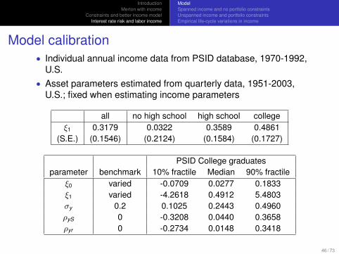
Model calibration• Individual annual income data from PSID database, 1970-1992,
U.S.• Asset parameters estimated from quarterly data, 1951-2003,
U.S.; fixed when estimating income parameters
all no high school high school collegeξ1 0.3179 0.0322 0.3589 0.4861
(S.E.) (0.1546) (0.2124) (0.1584) (0.1727)
PSID College graduatesparameter benchmark 10% fractile Median 90% fractile
ξ0 varied -0.0709 0.0277 0.1833ξ1 varied -4.2618 0.4912 5.4803σy 0.2 0.1025 0.2443 0.4960ρyS 0 -0.3208 0.0440 0.3658ρyr 0 -0.2734 0.0148 0.3418
46 / 73
IntroductionMerton with income
Constraints and better income modelInterest rate risk and labor income
ModelSpanned income and no portfolio constraintsUnspanned income and portfolio constraintsEmpirical life-cycle variations in income
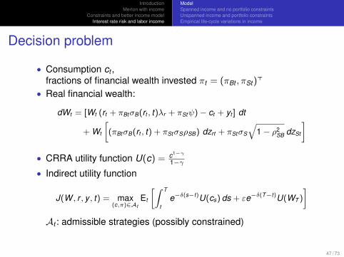
Decision problem
• Consumption ct ,fractions of financial wealth invested πt = (πBt , πSt )
>
• Real financial wealth:
dWt = [Wt (rt + πBtσB(rt , t)λr + πStψ)− ct + yt ] dt
+ Wt
[(πBtσB(rt , t) + πStσSρSB) dzrt + πStσS
√1− ρ2
SB dzSt
]• CRRA utility function U(c) = c1−γ
1−γ
• Indirect utility function
J(W , r , y , t) = max(c,π)∈At
Et
[∫ T
te−δ(s−t)U(cs) ds + εe−δ(T−t)U(WT )
]At : admissible strategies (possibly constrained)
47 / 73
IntroductionMerton with income
Constraints and better income modelInterest rate risk and labor income
ModelSpanned income and no portfolio constraintsUnspanned income and portfolio constraintsEmpirical life-cycle variations in income
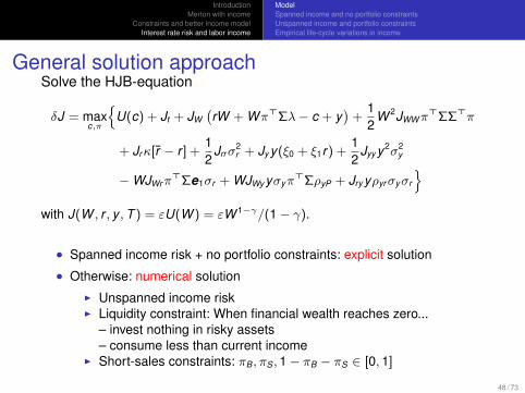
General solution approachSolve the HJB-equation
δJ = maxc,π
{U(c) + Jt + JW
(rW + Wπ>Σλ− c + y
)+
12
W 2JWWπ>ΣΣ>π
+ Jrκ[r − r ] +12
Jrrσ2r + Jy y(ξ0 + ξ1r) +
12
Jyy y2σ2y
−WJWrπ>Σe1σr + WJWy yσyπ
>ΣρyP + Jry yρyrσyσr
}with J(W , r , y ,T ) = εU(W ) = εW 1−γ/(1− γ).
• Spanned income risk + no portfolio constraints: explicit solution
• Otherwise: numerical solutionI Unspanned income riskI Liquidity constraint: When financial wealth reaches zero...
– invest nothing in risky assets– consume less than current income
I Short-sales constraints: πB, πS , 1− πB − πS ∈ [0, 1]
48 / 73
IntroductionMerton with income
Constraints and better income modelInterest rate risk and labor income
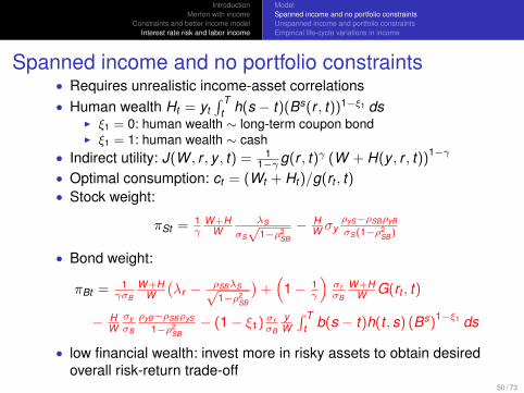
ModelSpanned income and no portfolio constraintsUnspanned income and portfolio constraintsEmpirical life-cycle variations in income
Spanned income and no portfolio constraints• Requires unrealistic income-asset correlations• Human wealth Ht = yt
∫ Tt h(s − t)(Bs(r , t))1−ξ1 ds
I ξ1 = 0: human wealth ∼ long-term coupon bondI ξ1 = 1: human wealth ∼ cash
• Indirect utility: J(W , r , y , t) = 11−γg(r , t)γ (W + H(y , r , t))1−γ
• Optimal consumption: ct = (Wt + Ht )/g(rt , t)• Stock weight:
πSt = 1γ
W +HW
λS
σS
√1−ρ2
SB
− HW σy
ρyS−ρSBρyB
σS(1−ρ2SB)
• Bond weight:
πBt = 1γσB
W +HW
(λr − ρSBλS√
1−ρ2SB
)+(
1− 1γ
)σrσB
W +HW G(rt , t)
− HWσyσB
ρyB−ρSBρyS
1−ρ2SB− (1− ξ1) σr
σB
yW
∫ Tt b(s − t)h(t , s) (Bs)1−ξ1 ds
• low financial wealth: invest more in risky assets to obtain desiredoverall risk-return trade-off
50 / 73
IntroductionMerton with income
Constraints and better income modelInterest rate risk and labor income
ModelSpanned income and no portfolio constraintsUnspanned income and portfolio constraintsEmpirical life-cycle variations in income
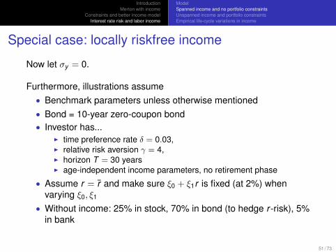
Special case: locally riskfree income
Now let σy = 0.
Furthermore, illustrations assume• Benchmark parameters unless otherwise mentioned• Bond = 10-year zero-coupon bond• Investor has...
I time preference rate δ = 0.03,I relative risk aversion γ = 4,I horizon T = 30 yearsI age-independent income parameters, no retirement phase
• Assume r = r and make sure ξ0 + ξ1r is fixed (at 2%) whenvarying ξ0, ξ1
• Without income: 25% in stock, 70% in bond (to hedge r -risk), 5%in bank
51 / 73
IntroductionMerton with income
Constraints and better income modelInterest rate risk and labor income
ModelSpanned income and no portfolio constraintsUnspanned income and portfolio constraintsEmpirical life-cycle variations in income
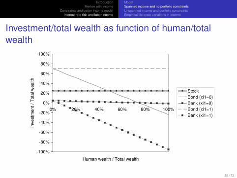
Investment/total wealth as function of human/totalwealth
-100%
-80%
-60%
-40%
-20%
0%
20%
40%
60%
80%
100%
0% 20% 40% 60% 80% 100%
Human wealth / Total wealth
Inve
stm
en
t /
Tota
l w
ealth
Stock
Bond (xi1=0)
Bank (xi1=0)
Bond (xi1=1)
Bank (xi1=1)
52 / 73
IntroductionMerton with income
Constraints and better income modelInterest rate risk and labor income
ModelSpanned income and no portfolio constraintsUnspanned income and portfolio constraintsEmpirical life-cycle variations in income
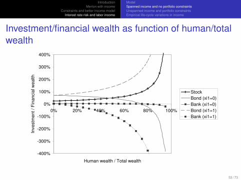
Investment/financial wealth as function of human/totalwealth
-400%
-300%
-200%
-100%
0%
100%
200%
300%
400%
0% 20% 40% 60% 80% 100%
Human wealth / Total wealth
Inve
stm
en
t /
Fin
ancia
l w
ea
lth
Stock
Bond (xi1=0)
Bank (xi1=0)
Bond (xi1=1)
Bank (xi1=1)
53 / 73
IntroductionMerton with income
Constraints and better income modelInterest rate risk and labor income
ModelSpanned income and no portfolio constraintsUnspanned income and portfolio constraintsEmpirical life-cycle variations in income
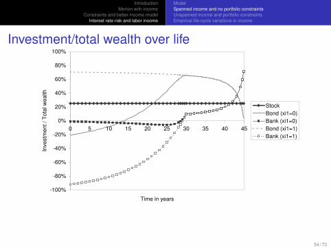
Investment/total wealth over life
-100%
-80%
-60%
-40%
-20%
0%
20%
40%
60%
80%
100%
0 5 10 15 20 25 30 35 40 45
Time in years
Inve
stm
en
t / T
ota
l w
ea
lth
Stock
Bond (xi1=0)
Bank (xi1=0)
Bond (xi1=1)
Bank (xi1=1)
54 / 73
IntroductionMerton with income
Constraints and better income modelInterest rate risk and labor income
ModelSpanned income and no portfolio constraintsUnspanned income and portfolio constraintsEmpirical life-cycle variations in income
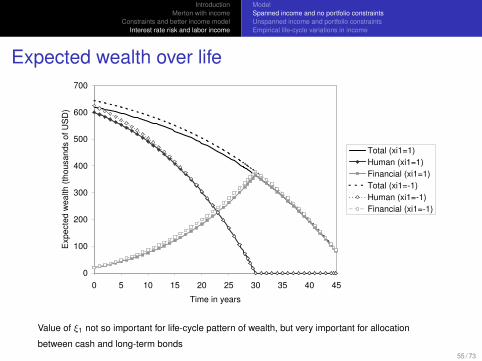
Expected wealth over life
0
100
200
300
400
500
600
700
0 5 10 15 20 25 30 35 40 45
Time in years
Exp
ecte
d w
ea
lth
(th
ou
sa
nd
s o
f U
SD
)
Total (xi1=1)
Human (xi1=1)
Financial (xi1=1)
Total (xi1=-1)
Human (xi1=-1)
Financial (xi1=-1)
Value of ξ1 not so important for life-cycle pattern of wealth, but very important for allocation
between cash and long-term bonds55 / 73
IntroductionMerton with income
Constraints and better income modelInterest rate risk and labor income
ModelSpanned income and no portfolio constraintsUnspanned income and portfolio constraintsEmpirical life-cycle variations in income
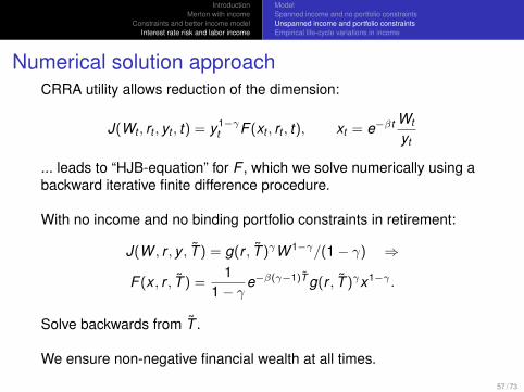
Numerical solution approachCRRA utility allows reduction of the dimension:
J(Wt , rt , yt , t) = y1−γt F (xt , rt , t), xt = e−βt Wt
yt
... leads to “HJB-equation” for F , which we solve numerically using abackward iterative finite difference procedure.
With no income and no binding portfolio constraints in retirement:
J(W , r , y , T ) = g(r , T )γW 1−γ/(1− γ) ⇒
F (x , r , T ) =1
1− γe−β(γ−1)T g(r , T )γx1−γ .
Solve backwards from T .
We ensure non-negative financial wealth at all times.
57 / 73
IntroductionMerton with income
Constraints and better income modelInterest rate risk and labor income
ModelSpanned income and no portfolio constraintsUnspanned income and portfolio constraintsEmpirical life-cycle variations in income
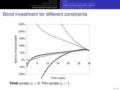
Bond investment for different constraints
-100%
-50%
0%
50%
100%
150%
200%
250%
0 5 10 15 20 25 30
Time in years
Bo
nd
in
v./
Fin
an
cia
l w
ea
lth
Thick curves: ξ1 = 0. Thin curves: ξ1 = 1.58 / 73
IntroductionMerton with income
Constraints and better income modelInterest rate risk and labor income
ModelSpanned income and no portfolio constraintsUnspanned income and portfolio constraintsEmpirical life-cycle variations in income
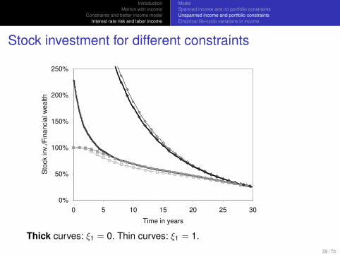
Stock investment for different constraints
0%
50%
100%
150%
200%
250%
0 5 10 15 20 25 30
Time in years
Sto
ck in
v./
Fin
an
cia
l w
ea
lth
Thick curves: ξ1 = 0. Thin curves: ξ1 = 1.59 / 73
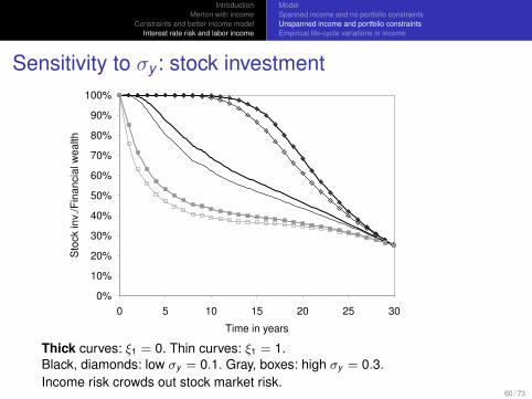
IntroductionMerton with income
Constraints and better income modelInterest rate risk and labor income
ModelSpanned income and no portfolio constraintsUnspanned income and portfolio constraintsEmpirical life-cycle variations in income
Sensitivity to σy : stock investment
0%
10%
20%
30%
40%
50%
60%
70%
80%
90%
100%
0 5 10 15 20 25 30
Time in years
Sto
ck in
v./
Fin
an
cia
l w
ea
lth
Thick curves: ξ1 = 0. Thin curves: ξ1 = 1.Black, diamonds: low σy = 0.1. Gray, boxes: high σy = 0.3.Income risk crowds out stock market risk.
60 / 73
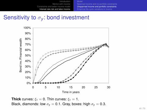
IntroductionMerton with income
Constraints and better income modelInterest rate risk and labor income
ModelSpanned income and no portfolio constraintsUnspanned income and portfolio constraintsEmpirical life-cycle variations in income
Sensitivity to σy : bond investment
0%
10%
20%
30%
40%
50%
60%
70%
80%
90%
100%
0 5 10 15 20 25 30
Time in years
Bo
nd
in
v./
Fin
an
cia
l w
ea
lth
Thick curves: ξ1 = 0. Thin curves: ξ1 = 1.Black, diamonds: low σy = 0.1. Gray, boxes: high σy = 0.3.
61 / 73
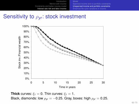
IntroductionMerton with income
Constraints and better income modelInterest rate risk and labor income
ModelSpanned income and no portfolio constraintsUnspanned income and portfolio constraintsEmpirical life-cycle variations in income
Sensitivity to ρyr : stock investment
0%
10%
20%
30%
40%
50%
60%
70%
80%
90%
100%
0 5 10 15 20 25 30
Time in years
Sto
ck in
v./
Fin
an
cia
l w
ea
lth
Thick curves: ξ1 = 0. Thin curves: ξ1 = 1.Black, diamonds: low ρyr = −0.25. Gray, boxes: high ρyr = 0.25.
62 / 73
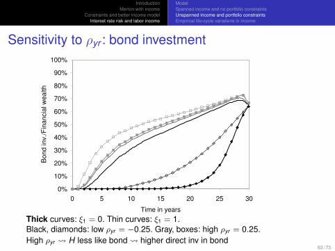
IntroductionMerton with income
Constraints and better income modelInterest rate risk and labor income
ModelSpanned income and no portfolio constraintsUnspanned income and portfolio constraintsEmpirical life-cycle variations in income
Sensitivity to ρyr : bond investment
0%
10%
20%
30%
40%
50%
60%
70%
80%
90%
100%
0 5 10 15 20 25 30
Time in years
Bo
nd
in
v./
Fin
an
cia
l w
ea
lth
Thick curves: ξ1 = 0. Thin curves: ξ1 = 1.Black, diamonds: low ρyr = −0.25. Gray, boxes: high ρyr = 0.25.High ρyr H less like bond higher direct inv in bond
63 / 73
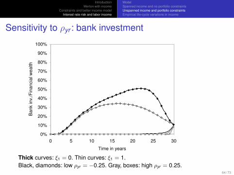
IntroductionMerton with income
Constraints and better income modelInterest rate risk and labor income
ModelSpanned income and no portfolio constraintsUnspanned income and portfolio constraintsEmpirical life-cycle variations in income
Sensitivity to ρyr : bank investment
0%
10%
20%
30%
40%
50%
60%
70%
80%
90%
100%
0 5 10 15 20 25 30
Time in years
Ba
nk in
v./
Fin
an
cia
l w
ea
lth
Thick curves: ξ1 = 0. Thin curves: ξ1 = 1.Black, diamonds: low ρyr = −0.25. Gray, boxes: high ρyr = 0.25.
64 / 73
IntroductionMerton with income
Constraints and better income modelInterest rate risk and labor income
ModelSpanned income and no portfolio constraintsUnspanned income and portfolio constraintsEmpirical life-cycle variations in income
Sensitivity to ξ1: stock investment
0%
10%
20%
30%
40%
50%
60%
70%
80%
90%
100%
0 5 10 15 20 25 30
Time in years
Sto
ck inv./F
inancia
l w
ealth
Thick unmarked curve: high ξ1 = 4. Thin unmarked curve: ξ1 = −4.
65 / 73
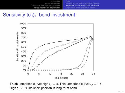
IntroductionMerton with income
Constraints and better income modelInterest rate risk and labor income
ModelSpanned income and no portfolio constraintsUnspanned income and portfolio constraintsEmpirical life-cycle variations in income
Sensitivity to ξ1: bond investment
0%
10%
20%
30%
40%
50%
60%
70%
80%
90%
100%
0 5 10 15 20 25 30
Time in years
Bo
nd
in
v./
Fin
an
cia
l w
ea
lth
Thick unmarked curve: high ξ1 = 4. Thin unmarked curve: ξ1 = −4.High ξ1 H like short position in long-term bond
66 / 73
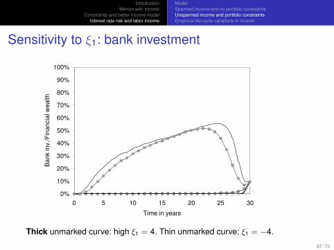
IntroductionMerton with income
Constraints and better income modelInterest rate risk and labor income
ModelSpanned income and no portfolio constraintsUnspanned income and portfolio constraintsEmpirical life-cycle variations in income
Sensitivity to ξ1: bank investment
0%
10%
20%
30%
40%
50%
60%
70%
80%
90%
100%
0 5 10 15 20 25 30
Time in years
Ba
nk in
v./
Fin
ancia
l w
ealth
Thick unmarked curve: high ξ1 = 4. Thin unmarked curve: ξ1 = −4.
67 / 73
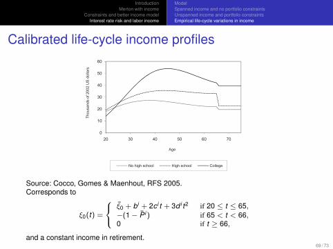
IntroductionMerton with income
Constraints and better income modelInterest rate risk and labor income
ModelSpanned income and no portfolio constraintsUnspanned income and portfolio constraintsEmpirical life-cycle variations in income
Calibrated life-cycle income profiles
10
20
30
40
50
60
Th
ou
sa
nd
s o
f 2
00
2 U
S d
olla
rs
0
10
20
30
40
50
60
20 30 40 50 60 70
Th
ou
sa
nd
s o
f 2
00
2 U
S d
olla
rs
Age
No high school High school College
Source: Cocco, Gomes & Maenhout, RFS 2005.Corresponds to
ξ0(t) =
ξ0 + bi + 2c i t + 3d i t2 if 20 ≤ t ≤ 65,−(1 − P i ) if 65 < t < 66,0 if t ≥ 66,
and a constant income in retirement.69 / 73
IntroductionMerton with income
Constraints and better income modelInterest rate risk and labor income
ModelSpanned income and no portfolio constraintsUnspanned income and portfolio constraintsEmpirical life-cycle variations in income
Optimal portfolio: no high school
0%
10%
20%
30%
40%
50%
60%
70%
80%
90%
100%
25 30 35 40 45 50 55 60 65 70 75 80
Age, years
Po
rtfo
lio w
eig
hts
Lower gray area: stock. White area: bond. Shaded area: bank.Note: based on ξ1 = 0.03 (median value for no high school).
70 / 73
IntroductionMerton with income
Constraints and better income modelInterest rate risk and labor income
ModelSpanned income and no portfolio constraintsUnspanned income and portfolio constraintsEmpirical life-cycle variations in income
Optimal portfolio: college degree
0%
10%
20%
30%
40%
50%
60%
70%
80%
90%
100%
25 30 35 40 45 50 55 60 65 70 75 80
Age, years
Po
rtfo
lio w
eig
hts
Lower gray area: stock. White area: bond. Shaded area: bank.Note: based on ξ1 = 0.49 (median value for college graduates)
71 / 73
IntroductionMerton with income
Constraints and better income modelInterest rate risk and labor income
ModelSpanned income and no portfolio constraintsUnspanned income and portfolio constraintsEmpirical life-cycle variations in income
Optimal portfolio: college degree, high ξ1 = 3
0%
10%
20%
30%
40%
50%
60%
70%
80%
90%
100%
25 30 35 40 45 50 55 60 65 70 75
Age, years
Po
rtfo
lio w
eig
hts
Lower gray area: stock. White area: bond. Shaded area: bank.
72 / 73
IntroductionMerton with income
Constraints and better income modelInterest rate risk and labor income
ModelSpanned income and no portfolio constraintsUnspanned income and portfolio constraintsEmpirical life-cycle variations in income
Optimal portfolio: college degree, low ξ1 = −3
0%
10%
20%
30%
40%
50%
60%
70%
80%
90%
100%
25 30 35 40 45 50 55 60 65 70 75
Age, years
Po
rtfo
lio w
eig
hts
Lower gray area: stock. White area: bond. Shaded area: bank.
73 / 73