Embed Size (px)
Citation preview
Dynamic Cybersecurity Modelling and Analysis
A thesis
submitted in partial fulfillment
of the requirements for the Degree
of
Doctor of Philosophy
in the
University of Canterbury
by
Simon Yusuf Enoch
Supervisor and Examining Committee
Dr. Dong Seong Kim Supervisor
Prof. Christian W. Probst External Examiner
Prof. Shui Yu External Examiner
Department of Computer Science and Software Engineering
University of Canterbury
2018


Abstract
It is difficult to assess the security of modern networks, such as Cloud and
software defined networks, because they are usually dynamic with configuration
changes (e.g., changes in topology, firewall rules, etc). Graphical security
models, such as Attack Graphs and Attack Trees, are widely used to
systematically analyse the security posture of network systems using various
security metrics. However, there are challenges in using them (i.e., the
graphical security models and security metrics) to assess the security of
dynamic networks. First, the existing graphical security models are unable
to capture dynamic changes occurring in the networks over time. As a result,
there is a lack of techniques to efficiently capture and manage the security
changes that are happening in dynamic networks.
Secondly, the existing security metrics which are used with the models are not
designed for the analysis of dynamic networks, and hence their effectiveness
to the dynamic changes in the network remains unclear. Moreover, they may
not quantitatively represent the changes in the security posture of the dynamic
networks.
Thirdly, finding the optimal security solution for the dynamic networks is a
difficult task due to their complexity and uncertainty of changes made. That is,
an optimal solution for the current network configuration may not be optimal
when the dynamic network changes in the future. As a result, it is difficult
to select the best set of security solutions to deploy for modern networks
that are dynamic. This thesis aims to address the aforementioned issues in
three primary goals: (1) to develop an adaptable graphical security model to
ii
capture changes in dynamic networks, (2) to develop new security metrics that
can effectively represent the security posture of dynamic networks, and (3) to
develop optimal security hardening selection methods for dynamic networks
taking into account multiple objectives and constraints.
To achieve the goal (1), two variant security models namely Temporal-
Hierarchical Attack Representation Model (T-HARM) and Time-Independent
HARM are proposed. The main idea behind the T-HARM is to capture and
assess the security posture of the dynamic network at every time t, where the
frequency of measurements could be time driven, event-driven or user-driven.
On the other hand, the Time-Independent HARM is developed to provide an
overview of the security posture of dynamic networks by aggregating all the
observed multiple security states (i.e., without showing the multiple GSMs
generated for every t).
To achieve the goal (2), first, a systematic classification of the different type
of network and security changes is presented. Based on the network changes,
an evaluation of the existing security metrics is performed in order to identify
which ones are suitable for the analysis of dynamic networks. Then, a new set
of security metrics for assessing dynamic networks is developed. The proposed
security metrics capture the dynamic changes that affect the security posture
of the networks.
To achieve the goal (3), an approach to select the best set of security
hardening solutions for dynamic networks given multiple constraints (e.g.,
limited budget and downtime) is developed. T-HARM with three dynamic
security metrics is used to evaluate the effectiveness of heterogeneous security
hardening options. In addition, multi-objectives genetics algorithm is adapted
to compute Pareto optimal deployment solutions that minimise security risk,
security costs and downtime of implementation of the hardening options. The
feasibility of the proposed approach is demonstrated in a real-world scenario by
taking into account both patchable and non-patchable vulnerabilities. Further,
a sensitivity analysis of the parameters of the genetic algorithm with respect to
iii
the dynamic networks are performed. Then, the results of the effect of varying
multiple network states on the optimal solutions obtained are shown.
In summary, the main contribution of this thesis are: (1) the development
of adaptable security models to capture and assess the security of dynamic
networks; (2) the evaluations of existing security metrics for the analysis
of dynamic networks; (3) the development of metrics for the quantitative
assessment of dynamic networks; and (4) the development of optimal defence
approaches for dynamic networks given multiple constraints.
iv
Publications Arising from this Thesis
A significant part of this thesis has been published or submitted for
publication in the peer-reviewed journals and conferences as listed in the
following.
1. Simon Yusuf Enoch, Mengmeng Ge, Jin B. Hong, Hani Alzaid and
Dong Seong Kim. A Systematic Evaluation of Cybersecurity Metrics
for Dynamic Networks. In Computer Networks, Elsevier, Vol. 144, pp
216-229, October 2018.
2. Simon Yusuf Enoch, Jin B. Hong and Dong Seong Kim. Time
Independent Security Analysis for Dynamic Networks using Graphical
Security Models. In Proceedings of the 17th IEEE International
Conference on Trust, Security and Privacy in Computing and
Communications (TrustCom-18), July 31st - August 3rd 2018, New York,
USA.
3. Simon Yusuf Enoch, Jin. B. Hong, Mengmeng Ge, Hani Alzaid and
Dong Seong Kim. Automated Security Investment Analysis of Dynamic
Networks. In Proceedings of the 2018 Australasian Information Security
Conference (AISC - 18), In ACSW, 2018, January 30 - February 2, 2018,
Brisbane, QLD, Australia.
4. Simon Yusuf Enoch, Mengmeng Ge, Jin B. Hong, Hani Alzaid and Dong
Seong Kim. Evaluating the Effectiveness of Security Metrics for Dynamic
Networks. In Proceedings of the 16th IEEE International Conference on
Trust, Security and Privacy in Computing and Communications August,
2017 (TrustCom-17), Sydney, Australia.
5. Simon Yusuf Enoch, Jin B. Hong, Mengmeng Ge and Dong Seong Kim.
Composite Metrics for Network Security Analysis. Software Networking
Journal, River Publishers, 2017. 1 (2017):137-160.
v

6. Simon Yusuf Enoch, Mengmeng Ge, Jin B. Hong, Huy Kang Kim, Paul
Kim and Dong Seong Kim. Security Modelling and Analysis of Dynamic
Enterprise Networks. In Proceedings of the 16th IEEE International
Conference on Computer and Information Technology, (CIT-16) Yanuca
Island, Fiji, December 7-10, Dec. 2016.
7. Simon Yusuf Enoch, Jin B. Hong, Mengmeng Ge, Khaled MD. Khan
and Dong Seong Kim. Multi-Objective Security Hardening Optimisation
for Dynamic Networks, Submitted to the 53rd IEEE International
Conference on Communications (ICC-19), 20-24 May 2019 Shanghai,
China.
8. Jin B. Hong, Simon Yusuf Enoch, Dong Seong Kim and Khaled MD.
Khan. Stateless Security Risk Assessment for Dynamic Networks. In
Proceedings of the 48th Annual IEEE/IFIP International Conference on
Dependable Systems and Networks (DSN-18) (fast abstract), June 2018,
Luxembourg.
9. Jin B. Hong, Simon Yusuf Enoch, Dong Seong Kim, Armstrong
Nhlabatsi, Noora Fetais and Khaled MD. Khan. Dynamic Security
Metrics for Measuring the Effectiveness of Moving Target Defense
Techniques. In Computer & Security, Elsevier, Vol. 79, pp 33-52,
November 2018.
vi

Dedicated to my parents, Mr. and Mrs. Yusuf Enochson for all their
sacrifices.
vii

Acknowledgement
First and foremost, I am most grateful to God Almighty for His wisdom,
grace, and succour throughout my studies.
In the following, I would like to recognise individuals who helped me
throughout this research adventure.
I am incredibly grateful to my research supervisor Dr. Dong Seong Kim
for giving me the opportunity to do Ph.D. with him. Dr. Kim has not only
provided me with ideas for my research work, but he has also supported me
in all the aspects of my stay in New Zealand. Most specifically, I appreciate
all the time he has spent discussing my research work, editing my papers and
providing support for me to attend conferences. Thank you, and I will forever
remain grateful for this tremendous support and generosity.
I am also deeply thankful to Dr. Jin Hong for his comments, ideas, reviews,
advise, and lots more since the beginning of my Ph.D. studies and to the
end. Jin has provided me with the detailed explanation of many things about
security modelling and analysis. I am thankful to him especially for opening
his door to me every time that I am stuck during my studies.
Special gratitude goes to my past lab-mate Dr. Mengmeng Ge for the research
collaborations, stimulating discussions, continuous encouragement and her
support for meeting many deadlines. Also, I will like to thank the entire
members of the UC Cybersecurity Lab, Paul, Dilli, Matthew, Sophie, Sultan,
Bilal, Abdul and Julio for all the fun time we have had in the past years. Thank
you to Dibash, Prerna, Tieta, Enos and Geela for all the interesting random
talk we have had all these times (it was stress relieving).
viii

Thank you to all the staff of the Department, especially Dr. Walter
Guttman for agreeing to be my Associate Supervisor, and to the technicians,
for their timely help on any technical problem arising from my research. Thank
you to Alex, Lynleigh and Sharon for solving all my enquiries on conferences
and other matters.
Thank you to Solomon, Andy, John, Murna, Aliyu, Bulama and the
Nigerian community in Christchurch for many interesting naija-made foods,
naija talks, and discussions.
I am also grateful to the funding sources that made this thesis possible. In
particular, I acknowledge the funding from the following; Tertiary Education
Trust Fund (TETFund) through the Federal University Kashere - Gombe,
Nigeria, the University of Canterbury (UC) - Department of Computer
Science and Software Engineering Conference Scholarship, the UC College of
Engineering tuition fee Scholarship, the G B Battersby-Trimble Scholarship
and Qatar National Research Fund (through Dr. Dong Seong Kim).
Last but not the least, I would like to thank my parents, siblings and friends
for their support, endless love, prayers and believing in me.
ix
Contents
Abstract ii
Dedication vii
Acknowledgement viii
List of Abbreviations 10
List of General Notations 13
1 Introduction 16
1.1 Problem Statement . . . . . . . . . . . . . . . . . . . . . . . . . 17
1.2 Research Questions and Goals . . . . . . . . . . . . . . . . . . . 18
1.3 Methodology . . . . . . . . . . . . . . . . . . . . . . . . . . . . 19
1.4 Research Contributions . . . . . . . . . . . . . . . . . . . . . . . 21
1.5 Thesis Structure . . . . . . . . . . . . . . . . . . . . . . . . . . . 22
2 Literature Review 24
2.1 Graphical Security Models . . . . . . . . . . . . . . . . . . . . . 24
2.1.1 GSMs for Static Networks . . . . . . . . . . . . . . . . . 25
2.1.2 Dynamic Models for Dynamic Networks . . . . . . . . . 26
2.1.3 Graphical Security Models for Security Investment Analysis 28
2.2 Security Metrics . . . . . . . . . . . . . . . . . . . . . . . . . . . 30
2.2.1 Classification of Security Metrics . . . . . . . . . . . . . 33
2.3 Security Hardening Optimisation . . . . . . . . . . . . . . . . . 40
1

2.4 Summary . . . . . . . . . . . . . . . . . . . . . . . . . . . . . . 42
3 Temporal Graphical Security Model 43
3.1 Background on the HARM . . . . . . . . . . . . . . . . . . . . . 43
3.2 System and Attacker Model . . . . . . . . . . . . . . . . . . . . 44
3.2.1 System Model . . . . . . . . . . . . . . . . . . . . . . . . 45
3.2.2 Attacker Model . . . . . . . . . . . . . . . . . . . . . . . 46
3.3 Formalism of T-HARM . . . . . . . . . . . . . . . . . . . . . . . 47
3.3.1 Definitions of T-HARM . . . . . . . . . . . . . . . . . . 47
3.4 Changes in Dynamic Networks . . . . . . . . . . . . . . . . . . . 50
3.4.1 Categorisation of Network Changes . . . . . . . . . . . . 50
3.4.2 Formalism of Security Changes in T-HARM . . . . . . . 51
3.4.3 Construction of T-HARM: An Example . . . . . . . . . . 54
3.5 Summary . . . . . . . . . . . . . . . . . . . . . . . . . . . . . . 56
4 Dynamic Security Assessments 57
4.1 Composite Security Metrics . . . . . . . . . . . . . . . . . . . . 58
4.1.1 Impact on Attack Paths . . . . . . . . . . . . . . . . . . 58
4.1.2 Risk on Attack Paths . . . . . . . . . . . . . . . . . . . . 59
4.1.3 Probability of Attack Success on Paths . . . . . . . . . . 60
4.2 Evaluating the Effectiveness of Existing Security Metrics for
Dynamic Networks . . . . . . . . . . . . . . . . . . . . . . . . . 61
4.2.1 Security Metrics and their Computations . . . . . . . . . 61
4.2.2 Effective Patch Management using Prioritised Set of
Vulnerabilities . . . . . . . . . . . . . . . . . . . . . . . . 62
4.2.3 Simulation Network and Attacker Model . . . . . . . . . 64
4.3 Scenario Descriptions and Results . . . . . . . . . . . . . . . . . 66
4.3.1 Scenario I: Addition of Vulnerability . . . . . . . . . . . 67
4.3.2 Scenario II: Addition of Hosts . . . . . . . . . . . . . . . 69
4.3.3 Scenario III: Software Update . . . . . . . . . . . . . . . 72
4.3.4 Scenario IV: Disabling Application Software . . . . . . . 78
2
4.3.5 Scenario V: Installation of New Application . . . . . . . 81
4.3.6 Scenario VI: Removal of Hosts . . . . . . . . . . . . . . . 83
4.3.7 Scenario VII: Change of Firewall Rules . . . . . . . . . . 85
4.3.8 Summary of the Results . . . . . . . . . . . . . . . . . . 87
4.4 Security Investment Analysis of Dynamic Networks . . . . . . . 91
4.4.1 Single Loss Expectancy . . . . . . . . . . . . . . . . . . . 91
4.4.2 Periodic Loss Expectancy . . . . . . . . . . . . . . . . . 92
4.4.3 Benefit of Security . . . . . . . . . . . . . . . . . . . . . 92
4.4.4 Security Cost . . . . . . . . . . . . . . . . . . . . . . . . 93
4.4.5 Return on Security Investment . . . . . . . . . . . . . . . 93
4.4.6 Return on Attack . . . . . . . . . . . . . . . . . . . . . . 94
4.5 Defence Model . . . . . . . . . . . . . . . . . . . . . . . . . . . 95
4.6 Simulations and Results Analysis . . . . . . . . . . . . . . . . . 96
4.6.1 Scenario I . . . . . . . . . . . . . . . . . . . . . . . . . . 97
4.6.2 Scenario II . . . . . . . . . . . . . . . . . . . . . . . . . . 99
4.7 Summary . . . . . . . . . . . . . . . . . . . . . . . . . . . . . . 100
5 Time-Independent HARM 102
5.1 Network and Attacker Model . . . . . . . . . . . . . . . . . . . . 103
5.2 The Proposed Approach . . . . . . . . . . . . . . . . . . . . . . 105
5.2.1 Formalism of TI-HARM . . . . . . . . . . . . . . . . . . 106
5.2.2 Constructing TI-HARM . . . . . . . . . . . . . . . . . . 108
5.2.3 Security Metrics Calculations . . . . . . . . . . . . . . . 111
5.2.4 Determining the Minimum Weight Threshold to use for
TI-HARM . . . . . . . . . . . . . . . . . . . . . . . . . . 111
5.2.5 Security Rating System . . . . . . . . . . . . . . . . . . . 113
5.3 Simulations and Results . . . . . . . . . . . . . . . . . . . . . . 116
5.3.1 Scenario Description and Simulation Networks . . . . . . 116
5.3.2 Simulation Settings for the Network Models . . . . . . . 118
5.3.3 Results and Analysis . . . . . . . . . . . . . . . . . . . . 119
3

5.3.4 Computing the Minimal Weight Value to Use . . . . . . 124
5.4 Discussions . . . . . . . . . . . . . . . . . . . . . . . . . . . . . 125
5.5 Summary . . . . . . . . . . . . . . . . . . . . . . . . . . . . . . 126
6 Metrics for Assessing the Security of Dynamic Networks 127
6.1 Metrics for Assessing Dynamic Networks . . . . . . . . . . . . . 128
6.1.1 Dynamic Metrics . . . . . . . . . . . . . . . . . . . . . . 128
6.1.2 Stateless Metrics . . . . . . . . . . . . . . . . . . . . . . 138
6.1.3 Application of Dynamic Security Metric Modules . . . . 142
6.2 Simulations and Results . . . . . . . . . . . . . . . . . . . . . . 149
6.2.1 Varying the Number of Hosts . . . . . . . . . . . . . . . 150
6.2.2 Varying the Number of Vulnerabilities . . . . . . . . . . 152
6.2.3 Changing Edges (Topology) . . . . . . . . . . . . . . . . 153
6.3 Summary . . . . . . . . . . . . . . . . . . . . . . . . . . . . . . 153
7 Security Hardening Optimisation for Dynamic Networks 155
7.1 Proposed Approach . . . . . . . . . . . . . . . . . . . . . . . . . 156
7.1.1 Network Model . . . . . . . . . . . . . . . . . . . . . . . 157
7.1.2 The Defence Mechanism . . . . . . . . . . . . . . . . . . 157
7.1.3 Security Metrics . . . . . . . . . . . . . . . . . . . . . . . 160
7.1.4 Problem Formulation . . . . . . . . . . . . . . . . . . . . 161
7.1.5 The Optimisation Approach . . . . . . . . . . . . . . . . 163
7.2 Simulations and Results . . . . . . . . . . . . . . . . . . . . . . 164
7.2.1 Simulation Network . . . . . . . . . . . . . . . . . . . . . 165
7.2.2 Sensitivity Analysis . . . . . . . . . . . . . . . . . . . . . 170
7.2.3 Processing Time . . . . . . . . . . . . . . . . . . . . . . 171
7.2.4 Effect of Varying Network Properties: multiple states . . 173
7.3 Summary . . . . . . . . . . . . . . . . . . . . . . . . . . . . . . 175
8 Discussions and Future Work 177
8.1 Addressing the Research Questions . . . . . . . . . . . . . . . . 178
4

8.2 Limitations and Future Work . . . . . . . . . . . . . . . . . . . 179
8.2.1 Different network characteristics . . . . . . . . . . . . . . 180
8.2.2 Dynamic Models . . . . . . . . . . . . . . . . . . . . . . 180
8.2.3 Attacker Models . . . . . . . . . . . . . . . . . . . . . . 181
8.2.4 Security metrics . . . . . . . . . . . . . . . . . . . . . . . 181
8.2.5 Optimal Defence Models . . . . . . . . . . . . . . . . . . 182
8.2.6 Validation . . . . . . . . . . . . . . . . . . . . . . . . . . 183
9 Conclusions 184
References 187
5
List of Figures
2.1 Classification of security metrics. . . . . . . . . . . . . . . . . . 35
3.1 Configuration of the network. . . . . . . . . . . . . . . . . . . . 45
3.2 Example T-HARM when a change is detected (with T = 2) . . 55
4.1 Examples of composite security metrics. . . . . . . . . . . . . . 58
4.2 Addition of vulnerabilities . . . . . . . . . . . . . . . . . . . . . 68
4.3 Change with respect to addition of hosts . . . . . . . . . . . . . 71
4.4 Change with respect to emergence and patching of vulnerabilities 74
4.5 Change with respect to emergence and patching of
vulnerabilities with different PSV values for month 1 through
month 12, respectively . . . . . . . . . . . . . . . . . . . . . . . 76
4.6 Disabling a vulnerable application on a host . . . . . . . . . . . 80
4.7 Installing an application on a host . . . . . . . . . . . . . . . . . 82
4.8 Change with respect to removal of hosts . . . . . . . . . . . . . 84
4.9 Change with respect to firewall rules . . . . . . . . . . . . . . . 86
4.10 The use of several countermeasures when critical vulnerabilities
are found . . . . . . . . . . . . . . . . . . . . . . . . . . . . . . 97
5.1 Topology configurations for the network with pre-defined
changes that are captured at different time. The time window
T = 24 min. . . . . . . . . . . . . . . . . . . . . . . . . . . . . . 105
6
5.2 TI-HARM (a) TI-HARM with w = 0.0% (i.e., all the appearance
of components), (b) TI-HARM with w = 50%, and (c) TI-
HARM with w = 100% . . . . . . . . . . . . . . . . . . . . . . 112
5.3 Interpreting the SRS value . . . . . . . . . . . . . . . . . . . . . 115
5.4 The initial network use in simulations: (a) E - D - I network,
and (b) E - I network. . . . . . . . . . . . . . . . . . . . . . . . 117
5.5 The effect of increasing weight value on different network model 120
5.6 The effect of varying the number of states . . . . . . . . . . . . 122
5.7 The effect of varying the number of vulnerabilities . . . . . . . . 123
6.1 Metrics for assessing dynamic networks . . . . . . . . . . . . . . 129
6.2 Categorising attack efforts . . . . . . . . . . . . . . . . . . . . . 130
6.3 Categorising defence efforts . . . . . . . . . . . . . . . . . . . . 131
6.4 Topology configurations for the example network with pre-
defined changes that are captured at different time . . . . . . . 143
6.5 Varying the number of hosts . . . . . . . . . . . . . . . . . . . . 151
6.6 Varying the number of vulnerabilities . . . . . . . . . . . . . . . 152
6.7 Defence Effort: Changing edges . . . . . . . . . . . . . . . . . . 153
7.1 Topology configurations for the small-scale network, (a) ns0
topology: the initial network topology, (b) ns1 topology: host
U1 is disconnected from th network and WS1 is connected to
AS1, and (c) ns2 topology: host U1 is added back to the network.166
7.2 Final solutions . . . . . . . . . . . . . . . . . . . . . . . . . . . . 169
7.3 Changing the mutation probability . . . . . . . . . . . . . . . . 172
7.4 Runtime of the GA and the percentage accuracy with respect to
increasing population size and the number of generations . . . . 173
7.5 Changing the number of network states . . . . . . . . . . . . . . 175
7
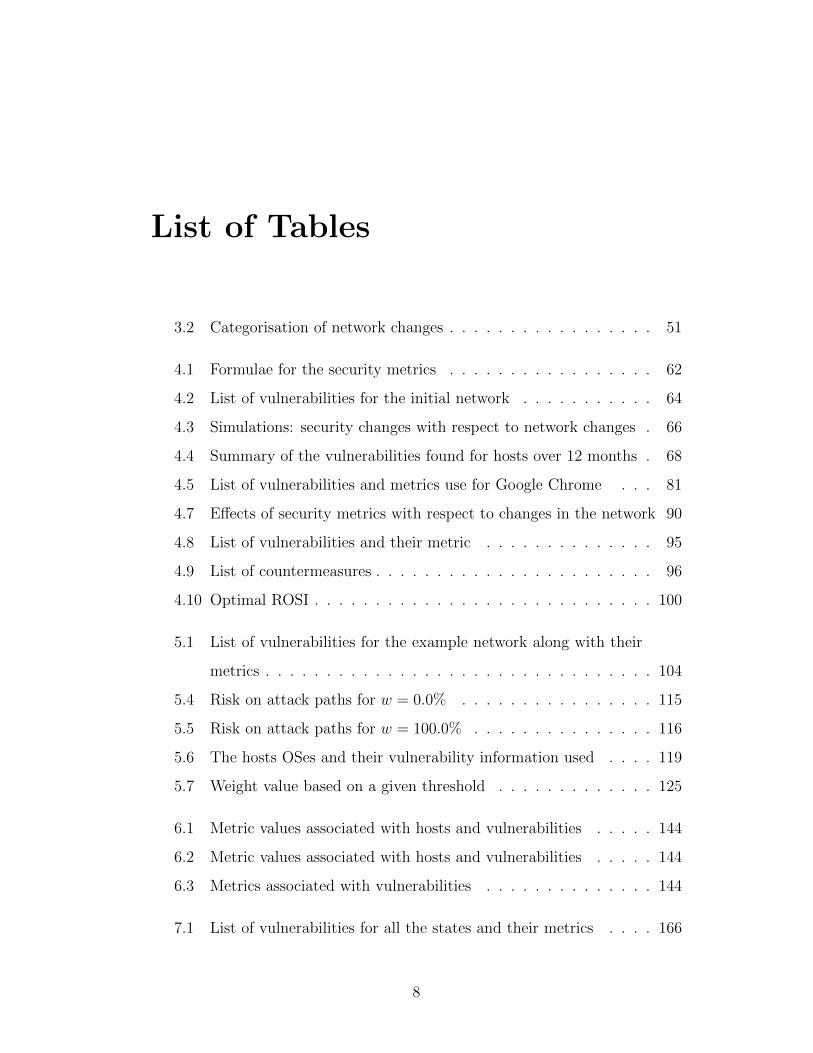
List of Tables
3.2 Categorisation of network changes . . . . . . . . . . . . . . . . . 51
4.1 Formulae for the security metrics . . . . . . . . . . . . . . . . . 62
4.2 List of vulnerabilities for the initial network . . . . . . . . . . . 64
4.3 Simulations: security changes with respect to network changes . 66
4.4 Summary of the vulnerabilities found for hosts over 12 months . 68
4.5 List of vulnerabilities and metrics use for Google Chrome . . . 81
4.7 Effects of security metrics with respect to changes in the network 90
4.8 List of vulnerabilities and their metric . . . . . . . . . . . . . . 95
4.9 List of countermeasures . . . . . . . . . . . . . . . . . . . . . . . 96
4.10 Optimal ROSI . . . . . . . . . . . . . . . . . . . . . . . . . . . . 100
5.1 List of vulnerabilities for the example network along with their
metrics . . . . . . . . . . . . . . . . . . . . . . . . . . . . . . . . 104
5.4 Risk on attack paths for w = 0.0% . . . . . . . . . . . . . . . . 115
5.5 Risk on attack paths for w = 100.0% . . . . . . . . . . . . . . . 116
5.6 The hosts OSes and their vulnerability information used . . . . 119
5.7 Weight value based on a given threshold . . . . . . . . . . . . . 125
6.1 Metric values associated with hosts and vulnerabilities . . . . . 144
6.2 Metric values associated with hosts and vulnerabilities . . . . . 144
6.3 Metrics associated with vulnerabilities . . . . . . . . . . . . . . 144
7.1 List of vulnerabilities for all the states and their metrics . . . . 166
8

7.2 changes in the network states with respect to the addition of
vulnerabilities . . . . . . . . . . . . . . . . . . . . . . . . . . . . 166
7.3 Hardening options costs . . . . . . . . . . . . . . . . . . . . . . 167
7.4 Security Stateless risk . . . . . . . . . . . . . . . . . . . . . . . . 168
7.5 The possible hardening options for each of the states . . . . . . 169
9
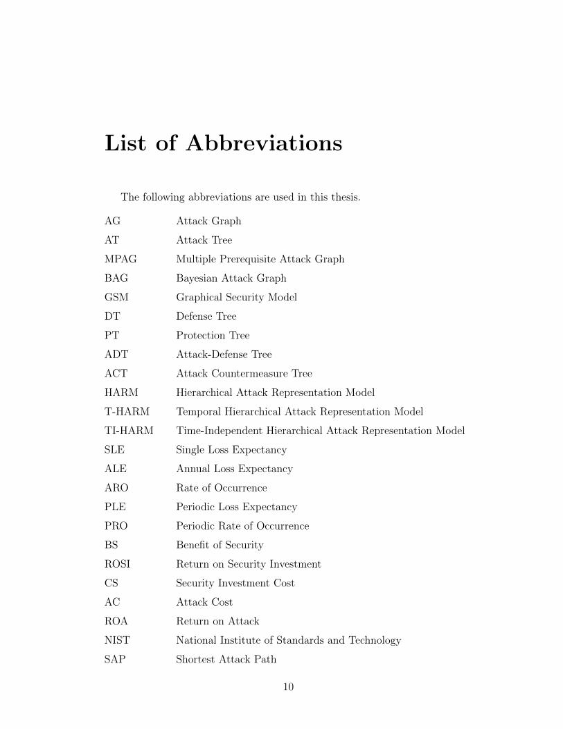
List of Abbreviations
The following abbreviations are used in this thesis.
AG Attack Graph
AT Attack Tree
MPAG Multiple Prerequisite Attack Graph
BAG Bayesian Attack Graph
GSM Graphical Security Model
DT Defense Tree
PT Protection Tree
ADT Attack-Defense Tree
ACT Attack Countermeasure Tree
HARM Hierarchical Attack Representation Model
T-HARM Temporal Hierarchical Attack Representation Model
TI-HARM Time-Independent Hierarchical Attack Representation Model
SLE Single Loss Expectancy
ALE Annual Loss Expectancy
ARO Rate of Occurrence
PLE Periodic Loss Expectancy
PRO Periodic Rate of Occurrence
BS Benefit of Security
ROSI Return on Security Investment
CS Security Investment Cost
AC Attack Cost
ROA Return on Attack
NIST National Institute of Standards and Technology
SAP Shortest Attack Path
10
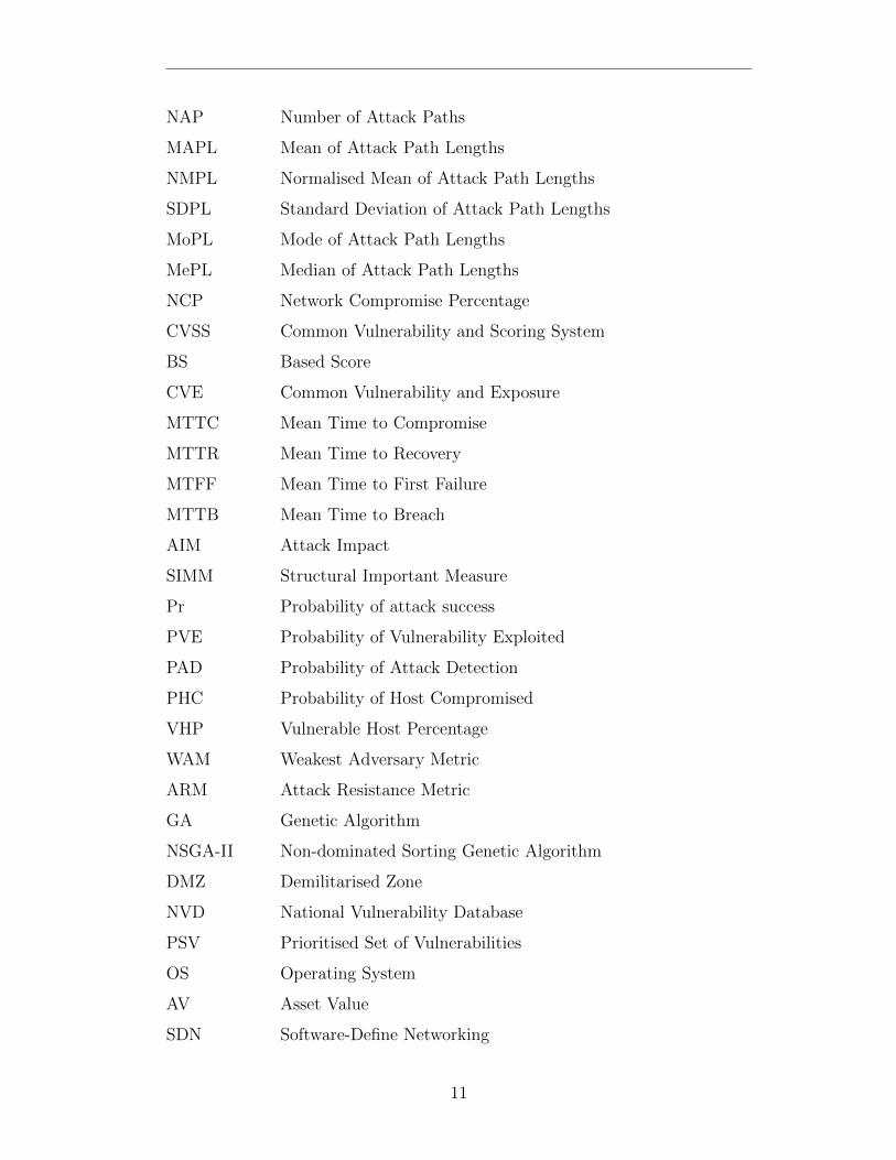
NAP Number of Attack Paths
MAPL Mean of Attack Path Lengths
NMPL Normalised Mean of Attack Path Lengths
SDPL Standard Deviation of Attack Path Lengths
MoPL Mode of Attack Path Lengths
MePL Median of Attack Path Lengths
NCP Network Compromise Percentage
CVSS Common Vulnerability and Scoring System
BS Based Score
CVE Common Vulnerability and Exposure
MTTC Mean Time to Compromise
MTTR Mean Time to Recovery
MTFF Mean Time to First Failure
MTTB Mean Time to Breach
AIM Attack Impact
SIMM Structural Important Measure
Pr Probability of attack success
PVE Probability of Vulnerability Exploited
PAD Probability of Attack Detection
PHC Probability of Host Compromised
VHP Vulnerable Host Percentage
WAM Weakest Adversary Metric
ARM Attack Resistance Metric
GA Genetic Algorithm
NSGA-II Non-dominated Sorting Genetic Algorithm
DMZ Demilitarised Zone
NVD National Vulnerability Database
PSV Prioritised Set of Vulnerabilities
OS Operating System
AV Asset Value
SDN Software-Define Networking
11

MWT Minimum Weight Threshold
MTD Moving Target Defence
BYOD Bring Your Own Device
APN Attack Path Number
APE Attack Path Exposure
ACE Attack Cost of Exploitability
ACD Attack Cost Duration
NDT Node Downtime
ECC Edge Changing Cost
ECT Edge Changing Time
SC Security Cost
PAP Persistent Attack Path Number
SR Stateless Risk
ISM Information Security Management
ARO Annualise Rate of Occurrence
SRS Security Rating System
PRO Periodic Rate of Occurrence
12
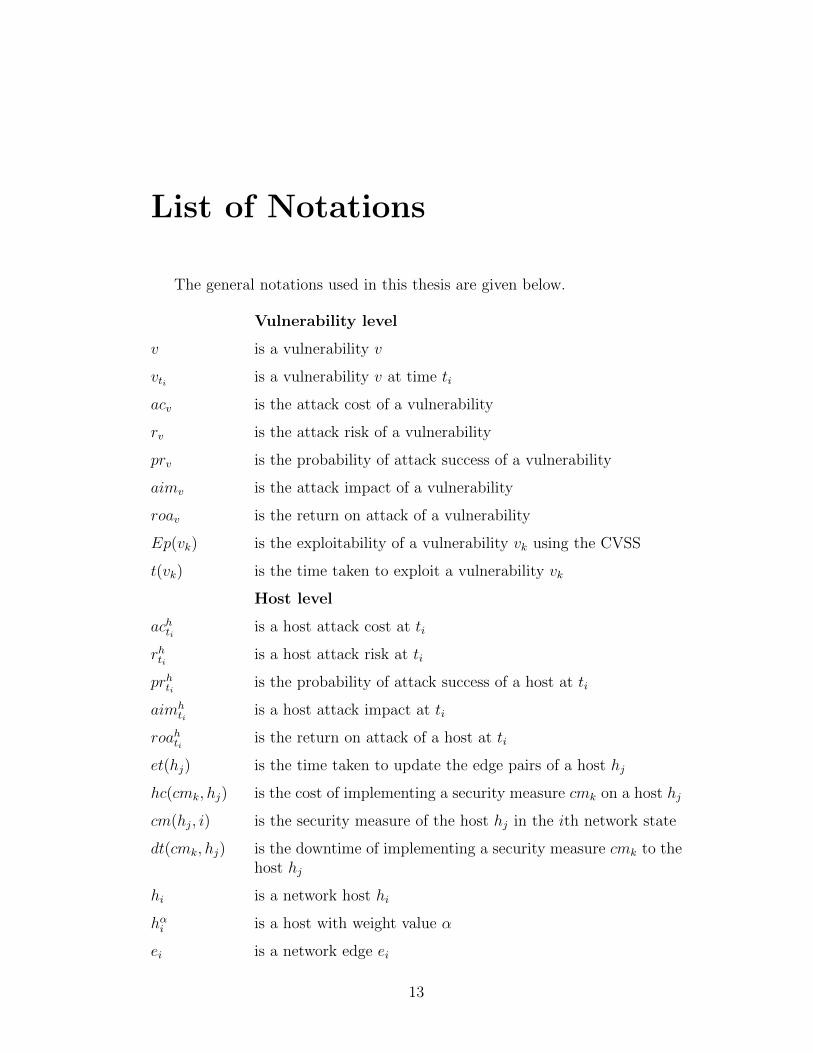
List of Notations
The general notations used in this thesis are given below.
Vulnerability level
v is a vulnerability v
vti is a vulnerability v at time ti
acv is the attack cost of a vulnerability
rv is the attack risk of a vulnerability
prv is the probability of attack success of a vulnerability
aimv is the attack impact of a vulnerability
roav is the return on attack of a vulnerability
Ep(vk) is the exploitability of a vulnerability vk using the CVSS
t(vk) is the time taken to exploit a vulnerability vk
Host level
achti is a host attack cost at ti
rhti is a host attack risk at ti
prhti is the probability of attack success of a host at ti
aimhti
is a host attack impact at ti
roahti is the return on attack of a host at ti
et(hj) is the time taken to update the edge pairs of a host hj
hc(cmk, hj) is the cost of implementing a security measure cmk on a host hj
cm(hj, i) is the security measure of the host hj in the ith network state
dt(cmk, hj) is the downtime of implementing a security measure cmk to thehost hj
hi is a network host hi
hαi is a host with weight value α
ei is a network edge ei
13

eαi is an edge with weight value α
ncαj is the weight value for a component ncj
Attack Path level
api is an attack path i which includes a sequence of hosts
acapiti is an attack path i which includes a sequence of hosts
rapiti is the attack risk on a path at ti
aimapiti is the attack impact on a path at ti
prapiti is the probability of attack success on a path at ti
roaapiti is the return on attack on a path at ti
t(api) is the time duration of an attack exploiting the attack path api
vuls(api) is the set of vulnerabilities associated with an attack path api
f is a function that identifies the length of the api that occursmost frequently
Network level
NS is a set of network states
AP is the set of attack paths for all the states
APnsti is all the possible paths from an attacker to a target for thenetwork state at ti. Each api ∈ APnsti
ACti is the cost on attack paths at ti
Rti is the risk on attack paths at ti
ROAti is return on attack paths at ti
Prti is the probability of attack success on paths at ti
AIMti is impact on attack paths at ti
SAPti is shortest attack path at ti
NAPti is the number of attack paths at ti
MAPLti is the mean of attack path lengths at ti
SDPLti is the standard deviation of attack path lengths at ti
MoPLti is mode of attack path lengths at ti
NMPLti is the normalised mean of attack path lengths at ti
PSSti is the percentage of severe systems at ti
NSSti is the number of severe systems at ti
TNHti is the total number of network hosts at ti
14

cmk is a of security hardening measure/countermeasure k
CM is a set of hardening security measure
t(nsti) is the time duration of a network state at ti
et(nsti) is the time duration of the edge pair changes in nsti
ncj is a network components ncj (e.g., hosts, edges)
OCncj is the observed count for ncj in a time window T
t(ncj) is the time duration of a network component ncj per state
w is the weight value threshold
15
Chapter 1
Introduction
Achieving security goals (i.e., Confidentiality, Integrity and Availability
[64]) for networked systems has long been a difficult task for many
organisations [117]. This has become even more difficult with modern network
technologies (such as Cloud and SDN) allowing their components to be more
dynamic with configuration changes over time. Such changes can be hosts
joining or disconnecting [106], applications and services update, vulnerability
added or removed [76], etc. As a result of these changes, the attack surface of
the network changes as well [19]. Therefore, it is of paramount importance to
assess the security of dynamic networks in order to understand how the security
posture changes, and also to effectively prevent damages caused by cyber-
attacks. To fully understand the security posture of the dynamic networks, one
must take into account all observable attributes of dynamic networks, which
includes changes of vulnerabilities, the visibility of hosts (components) over
time, the connectivity of network components (e.g., changes in host-to-host
reachability as a result of users’ activities), multiple network states, etc.
In this thesis, the term network states is used to represent different network
configurations and settings at various times. These configuration changes
include, but not limited to applications and OS changes, network topology
changes, vulnerability patches and other possible network configuration change.
16
Chapter 1. Introduction
1.1 Problem Statement
Graphical Security Models (e.g., AGs [3,127] and ATs [137,139]) are widely
used to assess the security of networks systematically [75,94] (the surveys in [75]
and [94] describes the whole family of GSMs with their various capabilities).
However, there are problems in the GSMs being applied to dynamic networks.
First, research on GSMs did not consider how the security assessment can
be affected when the network changes. As a result, it becomes difficult to
analyse the security of networks that are dynamic. Besides, they assumed
that GSMs use static information, e.g., vulnerabilities [105], the hosts, edges
(i.e., links connecting hosts), services running on the hosts, etc. However,
those components change over time (for example, the installation of a new
application software changes the attack surface by increasing the attack vectors
for the host [105]) and as such, the security analysis using those models is only
applicable for one particular state of the network. For dynamic networks with
frequent changes, the process of analysing only a single network state is not
comprehensive enough, especially for large-sized networks [74]. Therefore, it
needs an approach to efficiently model and analyse the security of the dynamic
network.
Secondly, many quantitative security metrics for assessing cybersecurity
have been developed and formalised [34,79,114,123,126,130,136]. While these
metrics remain useful in assessing the security of networks, their effectiveness
concerning dynamic changes in the network is still unclear. Moreover, those
metrics are not designed for the analysis of dynamic networks and thus, may not
be capable of representing the security posture of different states of the dynamic
networks. This is often crucial information for high-level decision makers to
understand the security overview without the technical details. Hence, it is
important to investigate how different security metrics are affected by changes
in the network, in order to identify which ones are suitable, or not suitable, for
security analysis of dynamic networks. Moreover, dynamic security metrics are
17

Chapter 1. Introduction
needed to capture the changing attack surface of dynamic networks in order to
provide effective security solutions.
Thirdly, the complexity and dynamicity of modern networks make it difficult
to select the best set of security hardening options to deploy. A security
hardening option refers to any strategy deployed to reduce an attacker’s ability
to compromise the security goals of networked systems. Here, as the network
configurations change, manually selecting the optimal security hardening
options becomes time-consuming and infeasible, especially when the size of the
dynamic network becomes larger. Moreover, security administrators often have
a limited security budget that restricts them from implementing all possible
security hardening options. Consequently, the security administrator needs to
select an optimal set of security hardening options, which will maximise the
security of the network under given constraints (e,g., taking into account a
limited security budget and various security objectives). Besides, computing
the optimum set of security hardening options for dynamic networks should
also be done within a feasible time frame. However, the solution search space
increases exponentially as the size of the network grows, as well as incorporating
the dynamic nature of the network components.
1.2 Research Questions and Goals
This thesis uses the security modelling approach to answer the following
questions:
� Q1: what are the approaches that be used to systematically capture and
model the attack scenarios in dynamic networks?
� Q2: what are the characteristics of dynamic networks, and how can we
quantitatively measure the security of the dynamic networks?
� Q3: what approach can be used to select the optimal security hardening
solutions for dynamic networks taking into account multiple objectives
18

Chapter 1. Introduction
(e.g., maximise security and minimise cost)?
The goals of this thesis are to advance the cybersecurity modelling and
assessment for the dynamic networks. Three sub-goals corresponding to the
research questions are described below:
� G1: To develop an adaptable graphical security model to capture security
changes in dynamic networks. The outcomes of this goal include new
security models to capture security changes over time, a formal definition
of its structure and functionality, and the classification of potential
network changes and their relationships to the possible security changes
(in the GSM).
� G2: To develop new security metrics that effectively represent the security
posture of dynamic networks. The outcomes of this goal consist of a
comprehensive evaluation of existing security metrics, classifications of
security metrics, a new approach to combining existing security metrics,
and new dynamic security metrics, and their formalisms.
� G3: To develop optimal security hardening selection methods for dynamic
networks taking into account multiple objectives and constraints. The
outcome of achieving this goal is a new approach to selecting a set of
security hardening options from a pool of potential security solutions for
dynamic networks while satisfying multiple objectives and constraints.
1.3 Methodology
In the following, the five phases to answer the proposed research questions
are described.
System Model: A dynamic enterprise network is used as the system
model, wherein there are subnets, firewalls, hosts (e.g., servers and users’
workstations), etc. It is assumed that the network has multiple states with each
network states having different network configurations (e.g., new hosts joining,
19
Chapter 1. Introduction
new vulnerabilities found, existing vulnerability patched, etc). Besides, it is
assumed that the changes in the network state are captured at various time or
when changes occur in the network (depending on the scenario). The changing
configurations information and the network states are used as input to the
security models and the metrics calculations.
Attacker Model: The attacker model provides the interactions between the
attacker and the system model. As the attacker model is needed for the
GSMs, this thesis assumed the attackers’ entry points, target and goals. Based
on the network hosts’ vulnerabilities and reachability information, the GSM
computes the potential attack scenarios with the assumptions that the attacker
can exploit the vulnerabilities. Also, it is assumed that the attacker can find
multiple attack paths to reach the target at any time.
Defence Model: Both the reactive and proactive defence mechanisms are used
for different network scenarios. These mechanisms can be deployed on either
the hosts level, the network level or on both levels. For example, a vulnerable
application can be disabled on a host (other types of the mechanisms such as
host isolation, traffic redirection, etc. are used as well) to mitigate against
exposure to attacks as a result of non-patchable vulnerability (i.e., the host
level).
GSMs: Security models are developed to capture and analyse the security
of dynamic networks. The security models use both the system model,
the attacker model and defence model (if there is) as input. The system
model provides the changing network reachability information and the hosts’
vulnerabilities explicitly over time, including the metrics for the vulnerabilities.
While the attacker model specifies the location of the attacker, the target, the
goal and the entry points for the attacker. The defence model specifies the
possible security hardening measure for the network.
Evaluation: Scenarios via simulations are used to evaluate the approaches.
The evaluation aims to show the feasibility of the proposed GSMs, security
metrics and the optimal defence selection mechanism developed.
20
Chapter 1. Introduction
1.4 Research Contributions
Five major contributions are proposed to the graphical security modelling
and analysis, which are as follows.
1. Development of a temporal graphical security model to capture and
analyse the security of dynamic networks at every time t (the work has
been published in [47, 48]). The temporal GSM captures the security
changes onto two layers at the various time; the temporal network
topology is captured at the upper layer using AGs and the vulnerability
information for each node at the lower layer using a set of ATs. By
doing so, the possible security of the network states can be captured and
analysed at the various time. Thus, showing the changes in the network
states at every time t.
2. Development of time-independent graphical security model that capture
all potential attack scenarios of dynamic networks regardless of network
states and time (the work has been published in [51]). The main idea of
the time-independent security model is to model the security of dynamic
networks by aggregating the security components of multiple states to
form a single GSM. By doing so, all the possible network components
observed in various network states can be captured, and thus allowing
us to model all possible attack scenarios including ones carried out in
multiple network states on a single GSM without having to look at
multiple GSMs. Moreover, the overall overview of the network security
(using metrics) can be calculated without looking at the multiple metrics
for every time t.
3. A systematic evaluation of cybersecurity metrics for the analysis of
dynamic networks (the work has been published in [46,49]). As of the time
of this research, there is no systematic evaluation of the existing security
metrics to determine their effectiveness for the analysis of dynamic
21
Chapter 1. Introduction
networks. In this thesis, the security metrics are evaluated based on
various network changes at the various time. The temporal GSM is used
to capture the security changes that happened as a result of the network
changes. Moreover, an approach to develop composite security metrics for
the analysis of network security is proposed (the work has been published
in [50]).
4. Development of dynamic security metrics to assess the security of
dynamic networks. New security metrics are developed to measure
the security posture of dynamic networks (part of this work has been
published in [70, 71]). As current security metrics are not designed for
dynamic networks, the changes in dynamic networks are characterised,
and based on the characteristics, the properties of metrics that will
capture the changes are identified in order to develop the new set of
dynamic metrics.
5. Development of optimal defence mechanisms for the dynamic networks
(the work has been submitted to IEEE ICC 2019 [52]). Several defence
mechanisms were considered in order to harden the security of dynamic
networks (the network is having a mix of patchable and non-patchable
vulnerability). A multi-objective optimisation algorithm is used to search
for the optimal solutions from the pools of security hardening options.
1.5 Thesis Structure
The rest of the thesis is organised as follows. Chapter 2 summarises the
related work on the GSM approaches for enterprise networks, security metrics
and security hardening optimisation methods. Chapter 3 present the propose
Temporal Hierarchical Security Model to improve the adaptability of existing
security models. The classifications and formalisms of network change with
respect to security changes are presented as well (addressing the research goal
22
Chapter 1. Introduction
G1). Chapter 4 described various real-world scenarios of networks changes,
and also present the results for the simulation studies conducted on the
effectiveness of the current security metrics for the analysis of dynamic networks
(this is towards addressing the research goal G2). Chapter 5 presents the
Time-Independent HARM to present the overview of the security of dynamic
networks (addressing the research goal G1). Chapter 6 develops a new set
of security metrics for assessing dynamic networks. Their formalisms and
quantifications (addressing the research goal G2). Chapter 7 provides the
proposed approach for multi-objective security hardening optimisation problem
of dynamic networks under multiple constraints (addressing the research goal
G3). Chapter 8 discusses the usability and limitations of the thesis and
highlights the possible directions for extensions. Finally, Chapter 9 concludes
the thesis.
23

Chapter 2
Literature Review
This chapter discusses the related work on GSMs, security metrics and
security optimisation. Section 2.1 discusses the GSMs used to analyse the
security of traditional networks and the dynamic networks. Section 2.2
discusses the current security metrics and provides the classifications of the
current security metrics. Section 2.3 presents the existing approaches on
the optimal selection of defence mechanisms for network systems. Section
2.4 summarises the challenges of the existing approaches and highlighted the
proposed approaches.
2.1 Graphical Security Models
A GSM is a tool for security assessment of real-life systems [94]. Most
popular applications domain are internet related attacks [103, 153], voting
systems [26, 99], supervisory control and data acquisition systems [27, 31],
online banking systems [43], etc. The interest of this thesis is using GSMs
for the analysis of cyber-attack and defence scenarios. In the following, they
are discussed in two aspects: GSMs for static networks and GSMs for dynamic
networks, respectively.
24

Chapter 2. Literature Review
2.1.1 GSMs for Static Networks
Several papers addressed the problem of assessing the security of network
systems using different approaches. In this section, the Graph-based, Tree-
based and the Hierarchical approaches are presented. The Graph-based
approach employ the graph structure to represent attack scenario. The Tree-
based approach models attack scenario in a tree-like structure. While the
Hierarchical approach models the attack scenarios onto multiple layers.
Graph-based models: One of the earlier work is presented in [131] where
an AG is proposed to model computer attacks. In particular, the AG is
used to show all possible sequences of attack steps to gain access to a target
using network reachability information and a set of vulnerability. Some
other graph-based approaches for assessing the security of network systems
include [3,63,79,81,87,127,149] etc. However, analysing all possible sequences
of attack paths using the AG has a scalability problem [65, 74, 75]. As a
result, various work proposed different approaches to improve the scalability
of the AG [30, 66, 127, 132, 159]. For instance, Homer et al. [66] proposed two
approaches. First, they proposed an approach that automatically identifies the
portions of an AG that is not important in understanding the core security
problems and subsequently, removed it. Secondly, they proposed an approach
that grouped similar attack steps which they said it represents the number and
type of security problems. On the other hand, Ingols et al. [82] proposed a
MPAG which grouped multiple subsets of nodes in order to reduce the size
of the AG. Even at that, the generation of the MPAG still suffers from the
scalability problem since modern networks have become very large and highly
dynamic [74].
Tree-based models: Another type of the GSMs is the tree-based models
such as AT in [40, 111, 139, 151] etc. The AT is a tree-like structure which
systematically presents attack scenario in a network with the target as the root
node and the different ways of reaching the target as leaf nodes. They are used
25
Chapter 2. Literature Review
to analyse the security of systems, but they cannot be generated from network
system specifications (e.g., using hosts reachability information to know how an
attacker can move from one host to another host (i.e., cannot capture the attack
paths information explicitly)) unless when logical connections (e.g., sequential
AND gates) are used for the tree-based models [68, 75]. Moreover, they also
suffer from the scalability problem.
Hierarchical models: In order to address the scalability problem in
the graph-based and tree-based model, a multi-layer security model named
HARM was proposed in [74] which simplifies the evaluation of all possible
attack scenarios. In particular, the work in [74] presented a three-layer HARM
where the reachability of network subnets is captured at the upper layer, the
host reachability information for each subnet is captured in the middle layer
(using an AG), and the vulnerability information is captured in the lower layer
(using an AT). Further, they showed that the scalability and the computational
complexity is improved when more layers (hierarchy) are used in the multi-layer
HARM.
With respect to this research, the major challenges with the approaches as
mentioned earlier is that they do not take into account the various changes
that happen in the network for their security analysis. However, modern
networks are now dynamic. For instance, a network attack surface changes
when a new host is connected to the network (e.g., bring your own device [106]),
update of software vulnerabilities [7], the discovery of new vulnerabilities [7,76],
firewall configuration and settings changed, etc and hence, those GSMs may
not effectively model and analyse the security of dynamic network since the
attack surface from scenarios may be changing.
2.1.2 Dynamic Models for Dynamic Networks
A few studies have focused on developing GSMs for assessing the security of
dynamic networks. Frigault et al. [56] proposed a dynamic Bayesian network-
based model to capture the evolving vulnerabilities in a network. It is a
26

Chapter 2. Literature Review
theoretical framework, and they expect it to be used for analysing the changing
security aspects of a network. Besides, it is limited to only changes in
vulnerabilities, as network changes (e.g., changes in topology which changes
the hosts reachability information) are not taken into account. Another similar
approach is BAG proposed by Poolsappasit et al. in [132], however, in the BAG,
they adopt the idea of Bayesian belief networks and AG to encode different
security conditions and the relationship between the various network states
and the possibility of exploiting those relationships as well. Almohri et al. [5]
presented a success measurement graph model where they analyse the chances
of attacks in the presence of uncertainties and further showed how to deploy
security and service across the dynamic network optimally.
A few research for the social network analysis [146] modelled the dynamic
network in different ways. For instance, Lerman et al. [100] modelled a dynamic
network by taking snapshots of every connected node at different times. They
used their model to assess the number of paths that exist over time in the
network. Moreover, they also used dynamic centrality metric to rank the
importance of each node (i.e., by how well connected they are over time to the
rest of the network). Similarly, Braha and Bar-Yam [22] studied how degree
centrality evolves in a dynamic network. They represented a dynamic network
by creating a time series of the network. They characterised the centrality of
nodes in the daily networks using the nodal “degree” (i.e., the number of nodes
a particular node is connected to). In their work, they found that the degree
of a node varied dramatically over time.
Kostakos [155] represented a dynamic network using temporal graphs (a
graph in which the components are active at a specific time). They defined some
metrics for temporal graphs (e.g., temporal proximity, temporal availability)
and analysed the relationship between nodes over time, and also finds the role
of each node in the temporal context of the entire network. Kempe et al.
proposed a temporal network model in which each edge is annotated with a
time label specifying the edge time (duration) of connection. In the model,
27
Chapter 2. Literature Review
each path needs to obey the time order of the appearance of the edges [91].
Casteigts et al. [28] used time-varying graphs (also known as temporal graphs)
to model and analyse dynamic networks using a unified framework which they
proposed. In their paper, they studied the evolution of network properties as
they dynamically change in a complex network system using network metrics.
Similarly, Wehmuth et al. [160] presented a unified finite time-varying graph
models for dynamic networks which represent several previous models proposed
in [25, 28, 54, 152]. Their proposed unified model allows one to model the
periodic behaviour of components in dynamic networks inherently. They also
showed how node, path and connections are processed in their model.
Santoro et al. [141] presented a time-varying graph and its formalism, in which
they concisely showed the network temporal concepts and their properties. In
addition, they analysed the behaviour of network properties (e.g., temporal
sub-graph, sequences of a static graph) during the lifetime of a time-varying
graph using network metrics (e.g., temporal centrality, temporal diameter).
2.1.3 Graphical Security Models for Security
Investment Analysis
Only a few studies have considered the evaluation of IT security investments
using GSMs and economic metrics. Bistarelli et al. [14] evaluated IT security
assets by using DTs (i.e., extended ATs) where they placed countermeasures
on each leaf of the AT. Further, they compute SLE, ALE, BS and ROSI.
Roy et al. [137] proposed ACT in which both attack scenarios and security
countermeasures are taken into account. In the ACT, countermeasures
(detection and mitigation) are also placed on every node and not only at
the leaf nodes. Roy et al. showed the practical usability of their approach
by computing CS, AC, ROA and ROSI. Baca and Petersen [9] developed an
extension of AT, where they began by evaluating and prioritising the attack
countermeasures, then assigning the countermeasures to the leaves of ATs. In
28

Chapter 2. Literature Review
their work, they automated the calculation of the countermeasures cost and
showed the effectiveness of the proposed automation. Edge et al. [45] proposed
a PT which is based on the AT. In the PT, they used a protection component
(i.e., countermeasure) for every leaf node of ATs to construct PTs. Further,
they showed how to compute the CS and the Pr.
Kordy et al. [93] proposed ADT which is an extended AT in which
countermeasures are used as a node and they are allowed to appear at any
level of AT. Ji et al. [88] used the ADT for risk assessment and countermeasures
evaluation for cyber-physical systems. They showed how they had evaluated
the performance of the ADT using the metric ROSI and ROA.
Ingols et al. [82] developed a tool named NetSPA (which is based on the
AG) which can capture all possible ways that an attacker can compromise the
targeted network (and used it for risk analysis). In [81], Ingols et al. extended
their earlier work by incorporating countermeasures. In particular, they added
personal firewalls at the host and the network level, and further, they added an
intrusion prevention systems and proxy firewalls for all network hosts. However,
they did not calculate any economic metrics for the countermeasures deployed.
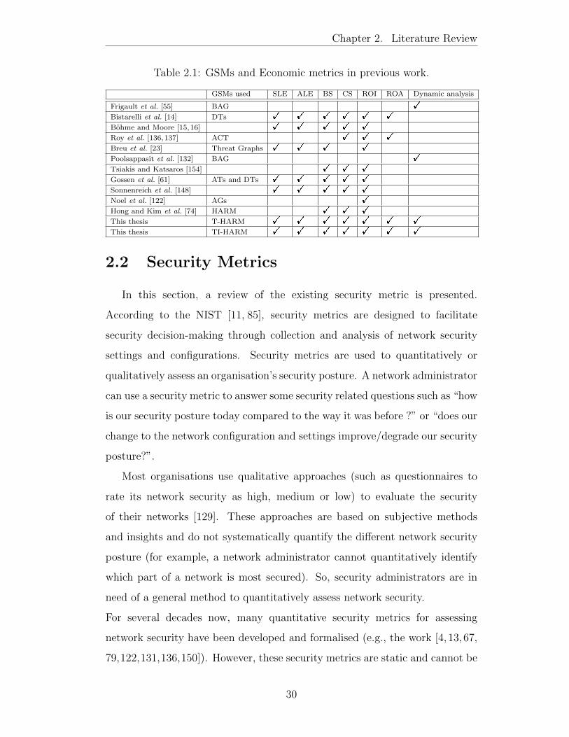
Table 2.1 summarises the most commonly used GSMs (where applicable)
and the economic metrics used in the previous work to automate security
investments analysis. From the table, only a few of the work automated
the computation of economic metrics, while the others described them (e.g.,
the work in [16, 33]). However, none of the previous work considered all the
following; (1) dynamic security analysis, (2) all economic metrics identified,
(3) the use of dynamic models and (4) the use of several countermeasures in
the GSM. Hence, this thesis automates the analysis of security investments
for changing networks using a dynamic GSM (T-HARM) along with various
economic metrics. In the table, !means it is considered.
29
Chapter 2. Literature Review
Table 2.1: GSMs and Economic metrics in previous work.
GSMs used SLE ALE BS CS ROI ROA Dynamic analysis
Frigault et al. [55] BAG !
Bistarelli et al. [14] DTs ! ! ! ! ! !
Bohme and Moore [15,16] ! ! ! ! !
Roy et al. [136,137] ACT ! ! !
Breu et al. [23] Threat Graphs ! ! ! !
Poolsappasit et al. [132] BAG !
Tsiakis and Katsaros [154] ! ! !
Gossen et al. [61] ATs and DTs ! ! ! ! !
Sonnenreich et al. [148] ! ! ! ! !
Noel et al. [122] AGs !
Hong and Kim et al. [74] HARM ! ! !
This thesis T-HARM ! ! ! ! ! ! !
This thesis TI-HARM ! ! ! ! ! ! !
2.2 Security Metrics
In this section, a review of the existing security metric is presented.
According to the NIST [11, 85], security metrics are designed to facilitate
security decision-making through collection and analysis of network security
settings and configurations. Security metrics are used to quantitatively or
qualitatively assess an organisation’s security posture. A network administrator
can use a security metric to answer some security related questions such as “how
is our security posture today compared to the way it was before ?” or “does our
change to the network configuration and settings improve/degrade our security
posture?”.
Most organisations use qualitative approaches (such as questionnaires to
rate its network security as high, medium or low) to evaluate the security
of their networks [129]. These approaches are based on subjective methods
and insights and do not systematically quantify the different network security
posture (for example, a network administrator cannot quantitatively identify
which part of a network is most secured). So, security administrators are in
need of a general method to quantitatively assess network security.
For several decades now, many quantitative security metrics for assessing
network security have been developed and formalised (e.g., the work [4,13,67,
79,122,131,136,150]). However, these security metrics are static and cannot be
30
Chapter 2. Literature Review
used to assess the security of a dynamic network [19]. For instance, Philips and
Swiler [131] proposed SAP metric, the metric presents the minimum amount
of effort an attacker needs to compromise a target. It is a metric from the
perspective of an attacker who has the options of different steps to compromise
a security policy.
Similarly, Pamula and Ammann [129] proposed the WAM that is based on the
analysis of AG. The metric assesses the security strength of a network in terms
of the attacker’s strength to successfully penetrate a network. These security
metrics are not effective security assessment metrics for dynamic networks
which are characterised by frequent topological changes [19]. This is because
the quantitative values produced by these metrics do not change even when
there is a topological change. Ortalo et al. [126] proposed the NAP metric to
assess the number of ways an attacker can compromise a target host. This
metric presents the total number of attack paths that can be available to the
attacker in order to launch an attack. Li and Vaughn [102] mention the average
attack path length metric (also called MAPL metric), they however, did not
describe nor formalise the metric but Idika and Bhargava described the metric
as the average of all attack path lengths and that the metric can be used
to shows the expected effort that an attacker may use to violate a security
countermeasure [79].
While all these metrics remains useful in assessing the security of networks,
they however cannot effectively assess the security of a dynamic network [19],
and this is because they were developed from the view of a static network (where
hosts and vulnerabilities information does not change). For example, in a
network, when the security status (e.g., vulnerability, reachability information)
of a host change, the structure of the AG changes also, when this occurs the
security has to be re-analysed as vulnerabilities and topology information have
changed. For dynamic networks with frequent changes, this process of re-
analysing the security becomes inefficient, especially for large sized networks.
Idika and Bhargava developed sets of AG-based metrics that assess the
31
Chapter 2. Literature Review
properties of a network in order to determine the network security. The metrics
are: the NMPL metric, the SDPL metric, the MoPL metrics and the MePL
metric [79]. The metrics are used to evaluate the different attributes of a
network’s security. Though the proposed security metrics were computed over
the whole AG, they are not able to capture the various security changes that
happen in a network over time [19].
The NCP is a metric developed by Lippmann et al. [104]. The NCP is the
percentage of the total assets across all hosts that have been captured by the
attacker. A value of zero indicates that no hosts have been compromised, and a
value of 100 indicates that all hosts have been compromised and all assets have
been captured. This metric is not useful in assessing the security of a dynamic
network because the NCP does not change even when a host vulnerability status
changes [124]. For example, if a host in the network has multiple vulnerabilities
and one of the host vulnerability is patched, the NCP does not change provided
there is at least one exploitable vulnerability remaining on the host.
There are also economic security metrics for assessing cybersecurity [13,17].
For instance, the AC [136] is a metric that quantity’s the cost spent by an
attacker to successfully exploit a vulnerability (i.e., security weakness) on a
host. The ROA [34] is also a security metric that is defined as the gain
the attacker expects from successful attack over the losses he sustains due
to the countermeasure deployed by his target. The return on attack is a
metric from the attacker perspective, and is used by organisations to evaluate
the effectiveness of a countermeasure and in discouraging a specific type of
intrusion attempts on a host. Bistarelli et al. [13] used the defender’s ROA and
the attacker’s ROA to evaluate the effectiveness of a countermeasure using DT
model. Roy et al. [136] used the AC metric and ROSI metric to perform security
analysis. Both studies did not consider the changing security components of
modern networks. Therefore, it is difficult to estimate how these metrics will
change as the network change over the period.
Bopche and Mehtre [19] proposed graph distance metrics which is based on
32
Chapter 2. Literature Review
maximum common subgraph and graph edit distance to measure the temporal
change in a dynamic network attack surface (an attack surface is a set of ways
that an attacker can use to penetrate a network system). They showed that
their proposed security metrics is able to capture the impact of events that
cause significant change in the network attack surface and also locate the most
vulnerable hosts in a dynamic network. Their proposed metric can only be
used to detect the changes that happen in a network attack surface and does
not maximise the granularity provided by the CVSS [36] in order to assess the
overall dynamic security in terms of risk, cost, impact, etc (e.g., risk analysis,
impact analysis). The CVSS is an industry open standard designed to convey
vulnerability severity and risk [35].
2.2.1 Classification of Security Metrics
There are a few research on the classification of security metrics. However,
most of the classification methods are based on organisation’s point of view
[143]. For instance, Savola [142] proposed three categories of security metrics;
namely, (i) business-level security metrics, (ii) metrics for ISM in organisations,
and (iii) dependability and trust metrics for products, systems and services.
The business-level security metrics are business goals directed and are used
for cost-benefit security analysis in organisations. The information security
management metrics are used to evaluate the ISM security controls, plans and
policies, and are divided into three subcategories (i.e., management, operational
and information system technical security metrics). The dependability and
trust metrics are used to assess the organisation’s trust, relationships and
dependability issues [8]. In general, this classification only addresses the
security needs of companies that produce information and telecommunication
technology products, systems or services.
Vaughn et al. [156] presented two categories of security metrics
(organisational security metrics and metrics for technical target assessment).
The organisational security metrics assess the organisation’s security
33
Chapter 2. Literature Review
assurance status (the metrics in this category include security effectiveness,
operational readiness for security incidents and information assurance program
development metric). The metrics for technical target assessment are used to
assess the security capabilities of a technical system (it is further divided into
metrics for strength assessment and metrics for weakness assessment [156]).
This classification is tailored towards an organisation’s needs.
Pendleton et al. [130] classified security metrics into four categories, namely:
metrics for measuring the system vulnerabilities, metrics for measuring the
defences, metrics for measuring the threats, and metrics for measuring the
situations. The metrics for measuring vulnerabilities are intended to quantify
the enterprise and computer systems vulnerabilities through their user’s
password, software vulnerabilities, and the vulnerabilities of the cryptographic
keys they use. The metrics for measuring defences is aimed to quantify the
countermeasure deployed in an enterprise via the effectiveness of blacklisting,
the ability of attack detection, the effectiveness of software diversification, and
the overall effectiveness of these countermeasures. The metrics for measuring
threats are aimed to assess the threats against an enterprise through the threat
of zero-day attacks, the power of individual attacks and the sophistication
of obfuscation. The metrics for measuring the situations aims to assess
situations via security investments, security states and security incidents. This
classification is centred on the perspective between attackers and defenders in
enterprise systems. Other classifications provided by industries such as the
NIST, the Center for Internet Security [33] and the Workshop on Information
Security System Scoring and Ranking are exclusively geared towards cyber
defence administrations and operations [130]. Here, a classification of
the existing security metrics based on network reachability information is
presented. Mainly, it is classified into two types: host-level metrics and
network-level metrics, as shown in Figure 2.1.
The host-level metrics do not use any network-level information (e.g.,
reachability, protocols, etc) whereas the network-level metrics take into account
34

Chapter 2. Literature Review
Figure 2.1: Classification of security metrics.
network structure, protocol and reachability information to quantify the
security of a system. The description of the host-level metrics given in Section
2.2.1.1 and the network-level metrics in Section 2.2.1.2, respectively.
2.2.1.1 Host-based Security Metrics
The host-level metrics are used to quantify the security level of individual
hosts in a network. It is classified into two types: “without probability” and
“with probability”. The reasons for this classification are: (i) sometimes it is
infeasible to find a probability value for an attack, and (ii) some analysis and
optimisation can be done with or without probability assignments as described
in [137].
Metrics without probability values:
The metrics “without probability” is summarise in Table 2.2. Examples of
metrics without probability values are AIM, AC, SIMM [136], mincut analysis
[136], MTTC [59, 101], MTTR [86], MTFF [140], MTTB [89], ROSI [34],
ROA [34], etc.
Metrics with probability values:
Conversely, the security metrics with probability include Pr [157], CVSS
metrics [36] etc. Wang et al. [157] proposed an AG-based security metric that
incorporates the likelihood of potential multi-step attacks combining multiple
vulnerabilities in order to reach the attack goal. We summarise the metrics
with probability in Table 2.3.
35
Chapter 2. Literature Review
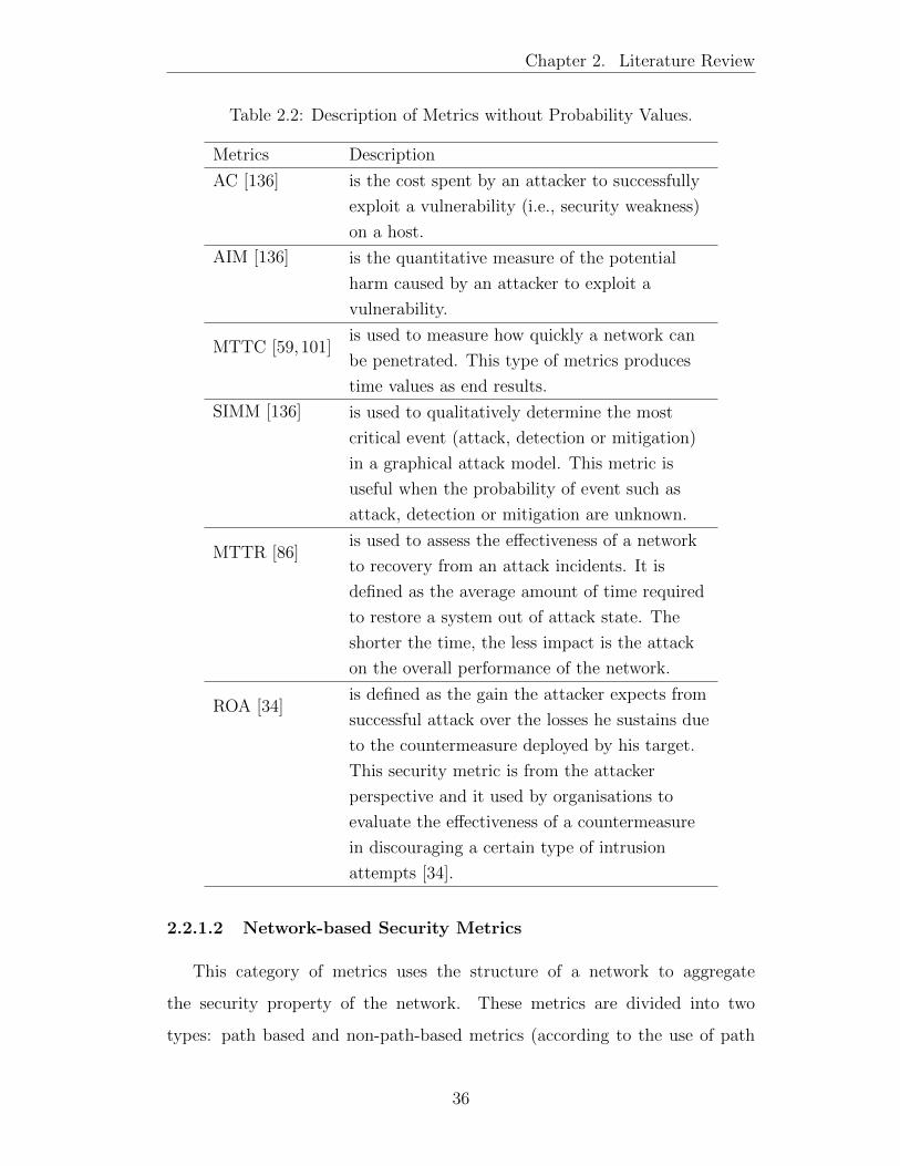
Table 2.2: Description of Metrics without Probability Values.
Metrics Description
AC [136] is the cost spent by an attacker to successfully
exploit a vulnerability (i.e., security weakness)
on a host.
AIM [136] is the quantitative measure of the potential
harm caused by an attacker to exploit a
vulnerability.
MTTC [59,101]is used to measure how quickly a network can
be penetrated. This type of metrics produces
time values as end results.
SIMM [136] is used to qualitatively determine the most
critical event (attack, detection or mitigation)
in a graphical attack model. This metric is
useful when the probability of event such as
attack, detection or mitigation are unknown.
MTTR [86]is used to assess the effectiveness of a network
to recovery from an attack incidents. It is
defined as the average amount of time required
to restore a system out of attack state. The
shorter the time, the less impact is the attack
on the overall performance of the network.
ROA [34]is defined as the gain the attacker expects from
successful attack over the losses he sustains due
to the countermeasure deployed by his target.
This security metric is from the attacker
perspective and it used by organisations to
evaluate the effectiveness of a countermeasure
in discouraging a certain type of intrusion
attempts [34].
2.2.1.2 Network-based Security Metrics
This category of metrics uses the structure of a network to aggregate
the security property of the network. These metrics are divided into two
types: path based and non-path-based metrics (according to the use of path
36
Chapter 2. Literature Review
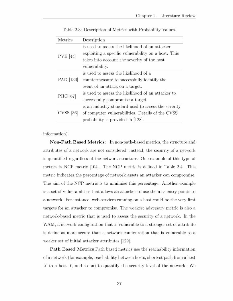
Table 2.3: Description of Metrics with Probability Values.
Metrics Description
PVE [44]
is used to assess the likelihood of an attacker
exploiting a specific vulnerability on a host. This
takes into account the severity of the host
vulnerability.
PAD [136]
is used to assess the likelihood of a
countermeasure to successfully identify the
event of an attack on a target.
PHC [67]is used to assess the likelihood of an attacker to
successfully compromise a target
CVSS [36]
is an industry standard used to assess the severity
of computer vulnerabilities. Details of the CVSS
probability is provided in [128].
information).
Non-Path Based Metrics: In non-path-based metrics, the structure and
attributes of a network are not considered; instead, the security of a network
is quantified regardless of the network structure. One example of this type of
metrics is NCP metric [104]. The NCP metric is defined in Table 2.4. This
metric indicates the percentage of network assets an attacker can compromise.
The aim of the NCP metric is to minimise this percentage. Another example
is a set of vulnerabilities that allows an attacker to use them as entry points to
a network. For instance, web-services running on a host could be the very first
targets for an attacker to compromise. The weakest adversary metric is also a
network-based metric that is used to assess the security of a network. In the
WAM, a network configuration that is vulnerable to a stronger set of attribute
is define as more secure than a network configuration that is vulnerable to a
weaker set of initial attacker attributes [129].
Path Based Metrics Path based metrics use the reachability information
of a network (for example, reachability between hosts, shortest path from a host
X to a host Y, and so on) to quantify the security level of the network. We
37
Chapter 2. Literature Review
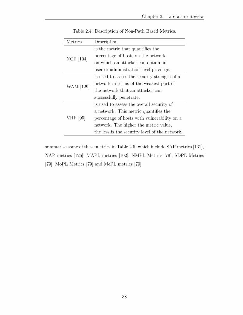
Table 2.4: Description of Non-Path Based Metrics.
Metrics Description
NCP [104]
is the metric that quantifies the
percentage of hosts on the network
on which an attacker can obtain an
user or administration level privilege.
WAM [129]
is used to assess the security strength of a
network in terms of the weakest part of
the network that an attacker can
successfully penetrate.
VHP [95]
is used to assess the overall security of
a network. This metric quantifies the
percentage of hosts with vulnerability on a
network. The higher the metric value,
the less is the security level of the network.
summarise some of these metrics in Table 2.5, which include SAP metrics [131],
NAP metrics [126], MAPL metrics [102], NMPL Metrics [79], SDPL Metrics
[79], MoPL Metrics [79] and MePL metrics [79].
38

Chapter 2. Literature Review
Table 2.5: Description of Path based Metrics.
Metrics Description
SAP [126,131]is the smallest distance from the attacker to the
target. This metric represents the minimum
number of hosts an attacker will use to
compromise the target host.
NAP [126]is the total number of ways an attacker can com-
promise the target. The higher the number, the
less secure the network.
MAPL [102]is the average of all path lengths. It gives the
expected effort that an attacker may use to
breach a network policy.
NMPL [79]This metric represents the expected number of
exploits an attacker should execute in order to
reach the target.
SDPL [79] is used to determine the attack paths of interest.
A path length that is two standard deviations
below the mean of path length metric is
considered the attack paths of interest and can
be recommended to the network administrator for
monitoring and consequently for patching.
MoPL [79] is the attack path length that occurs most
frequently. The Mode of Path Lengths metric
suggests a likely amount of effort an attacker
may encounter.
MePL [79] this metric is used by network administrator to
determine how close is an attack path length
to the value of the median path length (i.e. path
length that is at the middle of all the path
length values). The values that falls below the
median are monitored and considered for
network hardening.
ARM [159]is used to assess the resistance of a network confi-
guration based on the composition of measures of
individual exploits. It is also use for assessing and
comparing the security of different network
configurations.
39
Chapter 2. Literature Review
2.3 Security Hardening Optimisation
Various approaches have been proposed for the selection of security
hardening of networks. It is discussed as follows.
Jha et al. [87] used a greedy approach to find the minimal subset of hardening
options needed to secure the network from an attack using an AG. They
assumed that not all attack paths will be available to the attacker and therefore,
they applied hardening options on only a subset of attack scenario to achieve the
cost effectiveness. Phillips and Swiler [131] also used a greedy approach to find
a set of cost effective defence approaches. They incorporated cost (financial,
loss of services, etc.) and a defence budget into an AG in order to reduce
probability of attack success (or increase attack cost) for generating hardening
suggestions. Noel and Jajodia [121] used a greedy approach and an AG to find
the optimum placement of Intrusion Detection System sensors in a network
that will cover all critical attack paths. Idika et al. [80] modelled the problem
of selecting the best security options as a combinatorial optimisation problem.
They formulated the problem as a binary knapsack problem (i.e., the security
measures choosing problem) where the goal is to maximise security subject to
a limited budget. They used dynamic programming (with the binary knapsack
problem) to provide optimal solutions.
Kundu and Ghosh [97] modelled network hardening selection method
as a multi-objective optimisation problem with three objectives (minimise
cost, minimise risk and maximise overall network accessibility). They used
a multi-objective strategy search algorithm to select the optimum set of
security countermeasures under the given multiple constraints. Noel et al.
[122] proposed a network hardening option by computing the best network
reconfiguration options from the available reconfiguration options. Khanna
et al. [92] optimised the problem of deploying dynamic mobile sensors using
a multiple-objective genetic algorithm. Their approach optimally relocates
sensor host which further optimises host assignments, routes and attributes.
40
Chapter 2. Literature Review
Dewri et al. developed an approach to solve the problem of selecting optimum
security decision with multiple constraints via an AT. They used a genetic
algorithm [40] to select a subset of security hardening measures from a given set
such that the impact of attack damages and the total cost of countermeasure
implementation are minimised within a given budget. In [41], Dewri et al.
extended their earlier work by using the NSGA-II to find how security controls
can be placed in a network to induce a maximum return on investment. Borbor
et al. [20, 21] proposed a heterogeneous approach to select optimum set of
hardening options to deal with unknown and non-patchable vulnerabilities
under given cost constraints. They used GA and an extended resource graph
to solve this problem. However, all these approaches only considered the
optimisation problems based on static network configuration and settings.
Inspired by the work in [92] which uses GA to dynamically deploy secure
mobile sensors in a dynamic environment and the work in [21] which also
uses GA to consider heterogeneous hardening options for networks, the GA
is adapted to select optimum set of heterogeneous hardening options for the
dynamic networks (networks with multiple states). In particular, a NSGA-
II [110] is used. The NSGA-II has gained a lot of popularity for solving real
world problems (e.g., planning [144], scheduling [38], design [38]) because of
its effectiveness, ability to converge and ability to maintain a good distribution
over the objective functions [110].
The major difference between this work and the aforementioned approaches is
that the previous works rely on static network configuration information (where
there is no change in the network and security model) for their evaluations.
However, in this work, various dynamic network changes are considered (e.g.,
addition/removal of connections, addition of vulnerability, the availability of
a hardening option, etc). Moreover, dynamic security metrics are used to
evaluate the effectiveness of each defence option in the network.
41
Chapter 2. Literature Review
2.4 Summary
To address the aforementioned problems, the temporal graphs are
incorporated into the GSM to create T-HARM and TI-HARM to analyse the
security of ‘dynamic’ networks. Temporal graphs were mainly used to model
changes in the social network, but has not been used in the context of graphical
security models. The most obvious advantage of the proposed approach is
that it will effectively capture the network temporal change into two different
layers at different time (thereby, improving the adaptability of the current
approaches) and further, provides a way to analyse the security weaknesses
of a dynamic network. Moreover, it also provides an approach for the high
level decision makers to get the overview of the security of dynamic networks
without the technical details.
From the current research in security metrics, the researchers pay much
attention to security metrics for assessing the security of a network that does
not change, and the current security metrics are not proven to be effective to
assess the security of a dynamic network. Therefore, there is a need of metric to
effectively capture security changes and also quantitatively assess the security
strength of the dynamic network.
From the existing automated optimisation approaches for network systems,
most of the models relies on static network configurations and static security
metrics. On the other hand, one of the novelty of our work lies in the use
of automated security model with dynamic security metric to search for most
efficient solutions for the optimisation problem under multiple constraints.
42
Chapter 3
Temporal Graphical Security
Model
This chapter propose a temporal GSM named T-HARM. The T-HARM can
be used to capture and analyse the security properties of dynamic networks.
First, a brief background on the HARM is presented. Second, the descriptions
and formalisms of the T-HARM are presented. The main contributions of this
chapter are summarised as follows:
� Develop a temporal GSM, named T-HARM, to capture security changes
in dynamic networks;
� Formally define the T-HARM;
� Systematically categorise various network changes;
� Formally define the network changes with respect to the T-HARM;
3.1 Background on the HARM
To address the scalability problem of existing security models [3, 40, 63,
79, 81, 87, 111, 127, 139, 149, 151], Hong and Kim [74] developed a hierarchical
GSM. In particular, they developed a three-layer HARM where the reachability
43
Chapter 3. Temporal Graphical Security Model
of network subnets is captured at the upper layer, the host reachability
information for each subnet is captured in the middle layer (using an AG)
and the vulnerability information is captured in the lower layer (using an AT).
Hong and Kim used both the AG and the AT in the same model but on a
different layer to improve the scalability and the computational complexity of
GSMs.
However, the current approaches (including the HARM) do not take into
account the various changes that happen in the network for their security
analysis. But modern network changes frequently, for example, dynamic
networks consist of a varying set of hosts and edges (i.e., the connections
between the hosts) over time. Also, each of the hosts can have a varying set
of vulnerabilities which an attacker can use to compromise the hosts over the
time. As a result of these network changes, the attack vector for the network
changes frequently. Therefore, to effectively represent the changing security
posture of dynamic networks, GSMs need to adjust to changes when security
changes are observed in the networks. Hence, this chapter extends the static
HARM with the idea of temporal graphs to model the security changes of
dynamic networks.
3.2 System and Attacker Model
The system and the attacker model used to describe the T-HARM are
presented in Section 3.2.1 and Section 3.2.2, respectively. Specifically, the
system and the attacker models are used to incorporate the dynamic properties
of the network (i.e., how the system changes dynamically, and how the attack
scenarios are affected as a result). These models will be used in most part of
this thesis.
44
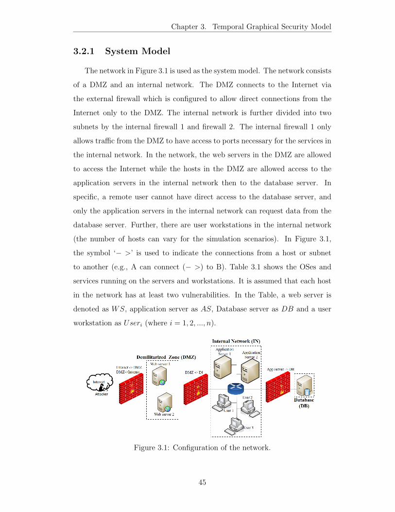
Chapter 3. Temporal Graphical Security Model
3.2.1 System Model
The network in Figure 3.1 is used as the system model. The network consists
of a DMZ and an internal network. The DMZ connects to the Internet via
the external firewall which is configured to allow direct connections from the
Internet only to the DMZ. The internal network is further divided into two
subnets by the internal firewall 1 and firewall 2. The internal firewall 1 only
allows traffic from the DMZ to have access to ports necessary for the services in
the internal network. In the network, the web servers in the DMZ are allowed
to access the Internet while the hosts in the DMZ are allowed access to the
application servers in the internal network then to the database server. In
specific, a remote user cannot have direct access to the database server, and
only the application servers in the internal network can request data from the
database server. Further, there are user workstations in the internal network
(the number of hosts can vary for the simulation scenarios). In Figure 3.1,
the symbol ‘− >’ is used to indicate the connections from a host or subnet
to another (e.g., A can connect (− >) to B). Table 3.1 shows the OSes and
services running on the servers and workstations. It is assumed that each host
in the network has at least two vulnerabilities. In the Table, a web server is
denoted as WS, application server as AS, Database server as DB and a user
workstation as Useri (where i = 1, 2, ..., n).
Figure 3.1: Configuration of the network.
45
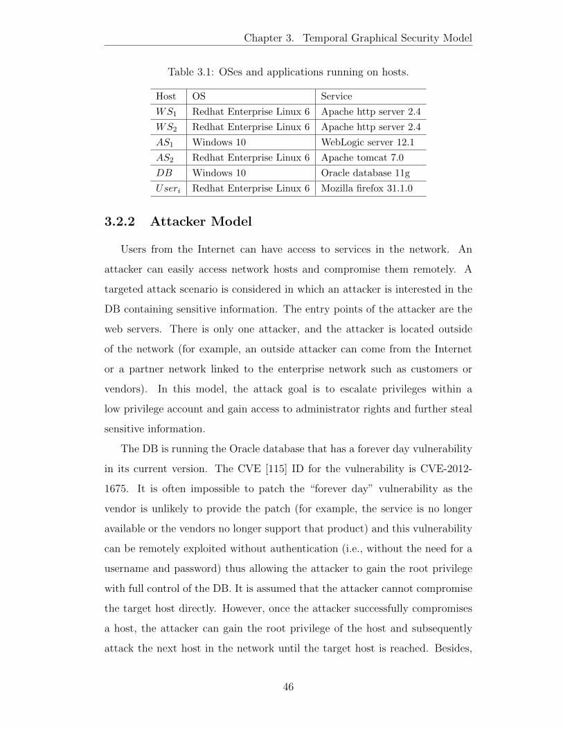
Chapter 3. Temporal Graphical Security Model
Table 3.1: OSes and applications running on hosts.
Host OS Service
WS1 Redhat Enterprise Linux 6 Apache http server 2.4
WS2 Redhat Enterprise Linux 6 Apache http server 2.4
AS1 Windows 10 WebLogic server 12.1
AS2 Redhat Enterprise Linux 6 Apache tomcat 7.0
DB Windows 10 Oracle database 11g
Useri Redhat Enterprise Linux 6 Mozilla firefox 31.1.0
3.2.2 Attacker Model
Users from the Internet can have access to services in the network. An
attacker can easily access network hosts and compromise them remotely. A
targeted attack scenario is considered in which an attacker is interested in the
DB containing sensitive information. The entry points of the attacker are the
web servers. There is only one attacker, and the attacker is located outside
of the network (for example, an outside attacker can come from the Internet
or a partner network linked to the enterprise network such as customers or
vendors). In this model, the attack goal is to escalate privileges within a
low privilege account and gain access to administrator rights and further steal
sensitive information.
The DB is running the Oracle database that has a forever day vulnerability
in its current version. The CVE [115] ID for the vulnerability is CVE-2012-
1675. It is often impossible to patch the “forever day” vulnerability as the
vendor is unlikely to provide the patch (for example, the service is no longer
available or the vendors no longer support that product) and this vulnerability
can be remotely exploited without authentication (i.e., without the need for a
username and password) thus allowing the attacker to gain the root privilege
with full control of the DB. It is assumed that the attacker cannot compromise
the target host directly. However, once the attacker successfully compromises
a host, the attacker can gain the root privilege of the host and subsequently
attack the next host in the network until the target host is reached. Besides,
46
Chapter 3. Temporal Graphical Security Model
the attacker must exploit vulnerabilities at the OS and the database level in
order to have full control of the target host (i.e., the DB).
3.3 Formalism of T-HARM
The main goal of the T-HARM is to analyse the security of dynamic
networks. Specifically, the T-HARM captures the security of network states
at varying times by constructing multiple HARMs for each time interval.
Moreover, it captures all the security changes onto two layers: the upper and the
lower layer. In the upper layer, the temporal hosts’ reachability information of
the hosts is captured while the changing vulnerabilities information is captured
in the lower layer.
3.3.1 Definitions of T-HARM
Given ti (where i = 1, 2, . . . , n), a discrete time in a time window T, the
T-HARM is define as follows.
Definition 1. T-HARM is a 3-tuple T − HARM = (S,H, V ), where S =
{st0 , st1 , . . . , stn} is a set of HARM for each network state at time ti, H =
{h0, h1, . . .} is a set of all hosts in the network, and V = {v0, v1, . . .} is a set of
all vulnerabilities in the network. Hti ⊆ H is a set of hosts only in the network
state at time ti, and Vti ⊆ V is a set of vulnerabilities only in the network state
at time ti.
In addition, the HARM for each discrete time ti is defined as follows.
Definition 2. A HARM at time ti is a 3-tuple sti = (Uti , Lti , Cti), where Uti is
the upper layer (dynamic AG) that models the set of hosts Hti, and Lti is the
lower layer (dynamic ATs) that models the set of vulnerabilities Vti for each
host h ∈ Hti, respectively. The mapping between the upper and the lower layers
is defined as Cti ⊆ {(hj ↔ atti,k)}∀hj ∈ Uti , atti,k ∈ Lti (here, k = 1, 2, . . .
denotes a distinct attack tree atti,k in the lower layer).
47

Chapter 3. Temporal Graphical Security Model
The attributes; the set of HARMs S, the set of hosts H, and the set of
vulnerabilities V are described as follows:
� Each HARM sti∈S has a set of hosts shoststi⊆Hti , a set of vulnerabilities
svulsti⊆Vti , a set of metrics smetricsti
∈{attack cost, attack risk, ROI, . . .}, a
topology information stopoti ∈{bus, tree, . . .}.
� Each host hj∈Hti has a set of adjacent hosts hadjj ⊆Hti , a set of
vulnerabilities hvj⊆Vti , and a set of security metrics hmetricsj ∈{attack cost,
attack risk, ROI, . . .}.
� Each vulnerability vk∈Vti has a privilege level that is acquired by the
attacker after the vulnerability is successfully exploited vprivilegek ∈{root,
user, ...} and a set of security metrics vmetricsk ∈{attack cost, attack risk,
. . .}.
Definition 3. A dynamic AG is a directed graph Uti = agti = (Hti , Eti) at
time ti, where Hti is a finite set of hosts and Eti⊆Hti×Hti is a set of edges.
Let Z be a sequence of attacker’s states which include one or multiple attackers
and z∈Z is a sequence of states zt0 , zt1 , ..., ztn, where n is the total number of
states, Z /∈S and Zhosts ∩ Hti = ∅. The representation of the upper layer is
given by Hti⊆S∪Z and Eti⊆(S∪Z)×S.
Definition 4. A dynamic AT is a 5-tuple atti,k=(Ati,k, Bti,k, cti,k, gti,k,
rootti,k),(Lti = {atti,1, atti,2, . . . atti,k, . . .}) at time ti. Here, Ati,k ⊆ Vti is a
set of vulnerabilities, Bti,k = {b1ti,k, b2ti,k, . . .} is a set of gates, cti,k ⊆ {b
jti,k→
el}∀bjti,k ∈ Bti,k, el ∈ Ati,k∪Bti,k is a mapping of gates to vulnerabilities and
other gates, gti,k ⊆ {bjti,k→{AND,OR}} specifies the type of each gate, and
rootti,k∈Ati,k∪Bti,k is the root node of the atti,k.
The gates {AND,OR} have relationships to vulnerabilities and other gates
that establish the connection cti,k (the vulnerability of a host are combined
using AND and OR gates). However, structuring the relationships between
the above components of the AT (i.e., gates and vulnerabilities) are outside
48
Chapter 3. Temporal Graphical Security Model
the scope of this thesis. The construct of the AT structures can be found
in [6, 77,145], which can be used to generate ATs used here.
Example 1. The mapping between the upper and lower layer components :
Figure 3.2 (the upper layer) shows T-HARM of the enterprise network when
a new host connect to the network. The T-HARM at time t2 is st2 =
(Ut2 , Lt2 , Ct2), where Ut2 and Lt2 are the AGs and the set of ATs in the
upper and the lower layer at t2, respectively, and Ct2 : Ut2→Lt2 is a one-to-
one mapping of the upper layer Ut2 to the corresponding lower layer Lt2 .
Example 2. The Upper Layer Components : At t2, the AG in the upper layer
is shown in Figure 3.2. The AG is a directed graph agt2 = (Ht2 , Et2), where
Ht2 ={A,WS1,WS2, User1, User2, User3, User4, AS1, AS2, DB} and Et2 =
{(A,WS1),(A,WS2),(WS1, User1),(WS1, AS1), (WS1, User2), (WS1, User3),
(WS1, User4), (WS2, User1), (WS2, User2), (WS2, User3), (WS2, User4),
(WS2, AS2), (User1, AS1), (User1, AS2), (User2, AS1),
(User2, AS2), (User3, AS1), (User3, AS2), (User4, AS1), (User4, AS2),
(AS1, DB), (AS2, DB)}.
Example 3. The Lower Layer Components : The ATs in the lower layer at
t2 is shown in Figure 3.2 (the lower layer). The set of conditions required to
compromise WS1 at t2 is given by att2,WS1=(At2,WS1 , Bt2,WS1 , ct2,WS1 , gt2,WS1 ,
roott2,WS1). Where At2,WS1 = {v8, v9} is a set of vulnerabilities for WS1,
Bt2,WS1 = OR1t2,WS1
, ct2,WS1 = {OR1t2,WS1
→ {v8, v9}} (i.e., the mapping of
gates to vulnerabilities and other gates), gt2,WS1 ⊆ {OR1t2,WS1
→{AND,OR}},
and roott2,WS1∈At2,WS1∪Bt2,WS1 is the root node of the att2,WS1 .
49
Chapter 3. Temporal Graphical Security Model
3.4 Changes in Dynamic Networks
In this section, a categorisation of network changes based on the causes of
configuration changes is proposed. Then, the T-HARM definition is extended
to include the formalism of the dynamic security changes as well (in Section
3.4.2).
3.4.1 Categorisation of Network Changes
In networks, there are hosts and edges (i.e., links connecting hosts). For each
host, there are applications and OS running on it and these components are
also with vulnerabilities (i.e., security weaknesses) [105]. The security status of
the hosts, edges, applications, OSes and vulnerabilities can be affected by the
activities of the users, network administrators and even other events not under
the control of the administrators (e.g., software ageing, the discovery of a new
vulnerability, etc). Hence, the network configuration is changing continuously.
Here, since changes in network configuration can change the security posture
of networks [19], the causes of network changes and the possible security
changes with respect to a GSM is identified and categorised into two main
categories which are; “change in host” and “change in edges (reachability)” (in
Table 3.2), respectively. The possible types of security changes are:
� (1) Addition of node (AN)
� (2) Removal of node (RN)
� (3) Addition of edge (AE)
� (4) Removal of edge (RE)
� (5) Addition of vulnerability (AV) and
� (6) Removal of vulnerability (RV)
50
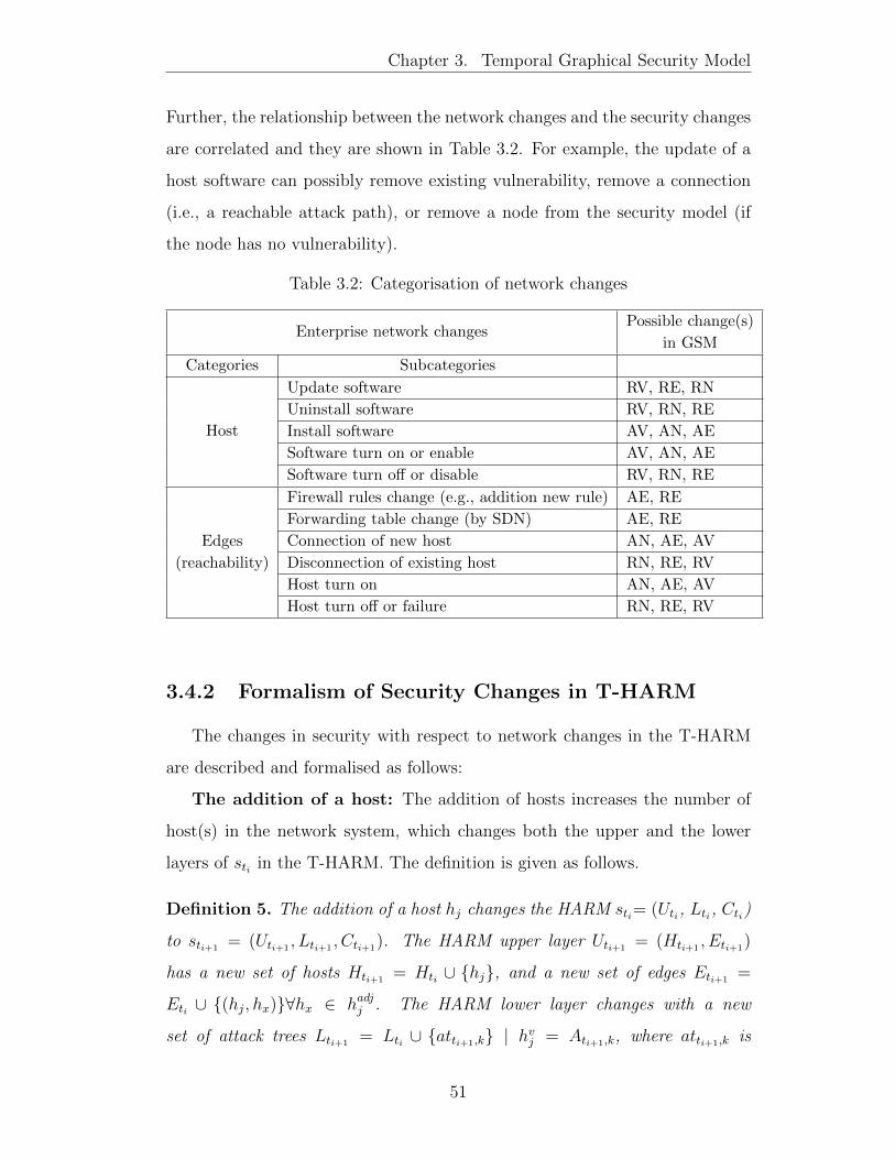
Chapter 3. Temporal Graphical Security Model
Further, the relationship between the network changes and the security changes
are correlated and they are shown in Table 3.2. For example, the update of a
host software can possibly remove existing vulnerability, remove a connection
(i.e., a reachable attack path), or remove a node from the security model (if
the node has no vulnerability).
Table 3.2: Categorisation of network changes
Enterprise network changesPossible change(s)
in GSM
Categories Subcategories
Host
Update software RV, RE, RN
Uninstall software RV, RN, RE
Install software AV, AN, AE
Software turn on or enable AV, AN, AE
Software turn off or disable RV, RN, RE
Edges
(reachability)
Firewall rules change (e.g., addition new rule) AE, RE
Forwarding table change (by SDN) AE, RE
Connection of new host AN, AE, AV
Disconnection of existing host RN, RE, RV
Host turn on AN, AE, AV
Host turn off or failure RN, RE, RV
3.4.2 Formalism of Security Changes in T-HARM
The changes in security with respect to network changes in the T-HARM
are described and formalised as follows:
The addition of a host: The addition of hosts increases the number of
host(s) in the network system, which changes both the upper and the lower
layers of sti in the T-HARM. The definition is given as follows.
Definition 5. The addition of a host hj changes the HARM sti= (Uti, Lti, Cti)
to sti+1= (Uti+1
, Lti+1, Cti+1
). The HARM upper layer Uti+1= (Hti+1
, Eti+1)
has a new set of hosts Hti+1= Hti ∪ {hj}, and a new set of edges Eti+1
=
Eti ∪ {(hj, hx)}∀hx ∈ hadjj . The HARM lower layer changes with a new
set of attack trees Lti+1= Lti ∪ {atti+1,k} | hvj = Ati+1,k, where atti+1,k is
51
Chapter 3. Temporal Graphical Security Model
a new attack tree that captures the vulnerabilities of hj. Lastly, the new
mapping between the upper and the lower layers of the HARM changes to
Cti+1= Cti ∪ {(hj ↔ atti+1,k)}.
The removal of a host: The removal of hosts reduces the number of hosts
in the network systems. When this happens, the reachability and vulnerabilities
associated with the hosts are removed as well. Thus, the upper and lower layers
of the T-HARM are changed. This is formally defined as:
Definition 6. The removal of a host hj changes the HARM sti= (Uti, Lti, Cti)
to sti+1= (Uti+1
, Lti+1, Cti+1
). The HARM upper layer Uti+1= (Hti+1
, Eti+1)
has a new set of hosts Hti+1= Hti − {hj}, and a new set of edges Eti+1
=
Eti − {(hj, hx)}∀hx ∈ hadjj . The HARM lower layer changes with a new set
of attack trees Lti+1= Lti − {atti,k}, where hj ↔ atti,k. Lastly, the new
mapping between the upper and the lower layers of the HARM changes to
Cti+1= Cti − {(hj ↔ atti,k)}.
The addition of a vulnerability: Given a new vulnerability vx, the AT
atti,k of a host hj where hj ↔ atti,k in Cti in the T-HARM at time ti is changed
when a new vulnerability is found for that host. The lower layer is changed in
the HARM, the list of vulnerabilities for the host is updated, and the set of
vulnerabilities at a time ti+1 is also updated. The definition is given as follows.
Definition 7. The addition of a vulnerability vx changes the AT atti,k of a
host hj with hj ↔ atti,k in Cti and vx ∈ hvj ⊆ Vti+1. This changes atti,k to
atti+1,k = (Ati+1,k, Bti+1,k, cti+1,k, gti+1,k, rootti+1,k), where Ati+1,k = Ati,k ∪ {vx}
(i.e., vx is added to the set of vulnerabilities), Bti+1,k = Bti,k∪{byti+1,k}
∀byti+1,k→el | el ∈ Ati+1,k∪Bti+1,k (i.e., new gates are added to connect other
vulnerabilities and gates with relation to vx), cti+1,k = cti,k∪{byti+1,k
→ el} where
el ∈ Ati+1,k∪Bti+1,k and el has a relation to vx. gti+1,k = gti,k (i.e., unchanged
set of gate types). Finally, rootti+1,k = ∈Ati+1,k∪Bti+1,k (i.e., may have a new
root node based on the relationship of vx). A list of vulnerabilities is updated
to Vti+1= Vti ∪ {vx}.
52
Chapter 3. Temporal Graphical Security Model
The removal of a vulnerability: Various event (e.g., applying security
countermeasures, uninstalling a vulnerable application, etc.) change the lower
layer of T-HARM. And as a result, it will need to be updated, and this change
is defined as:
Definition 8. The removal of a vulnerability vx from a host hj (where hj ↔
atti,k) will change the AT atti,k to atti+1,k = (Ati+1,k, Bti+1,k, cti+1,k, gti+1,k,
rootti+1,k), where Ati+1,k = Ati,k − {vx}, Bti+1,k = Bti,k−{byti+1,k} (i.e., if vx is
the only vulnerability associated with the gate), cti+1,k = cti,k − {byti+1,k
→ el}.
gti+1,k = gti,k (i.e., unchanged set of gate types). Finally, rootti+1,k = rootti,k.
A list of vulnerabilities is updated to Vti+1= Vti − {vx}.
The addition of an edge: An edge is created when there is a connection
between hosts. Hence, the set of edges is updated when a new connection
is created, and here, only the upper layer of T-HARM has changed. This is
defined as:
Definition 9. Given a new connection between hosts hj and hm at time ti+1.
The HARM sti is changed to sti+1= (Uti+1
, Lti+1, Cti+1
), where the upper layer
Uti+1= (Hti+1
, Eti+1) has a new edge such that Eti+1
= Eti ∪ {(hj, hm)},
Hti=Hti+1. Here, the lower layer Lti+1
= Lti and the mapping between the
upper layer to the lower layer Cti+1= Cti is unchanged.
The removal of an edge: Similarly, an edge is removed from hosts when
the reachability between them is disconnected. As a result, only the upper
layer of T-HARM is changed accordingly. The removal of edges is defined as
follows.
Definition 10. Given a connection between hosts hj and hm. The HARM
sti is changed to sti+1= (Uti+1
, Lti+1, Cti+1
), where the upper layer Uti+1=
(Hti+1, Eti+1
) is changed such that Eti+1= Eti − {(hj, hm)} and Hti+1
= Hti.
Here, the lower layer and the mapping between the upper layer to the lower
layer is unchanged (i.e., Lti+1= Lti and Cti+1
= Cti), respectively.
53
Chapter 3. Temporal Graphical Security Model
3.4.3 Construction of T-HARM: An Example
The T-HARM is used to capture network changes at different times. A
flexible time window can be assumed, so this can be adjusted to different time
and interval as desired (e.g., 5 hours or 1 day) thus providing a different view to
evaluate the security over time. An example T-HARM is shown in Figure 3.2
for the network shown in Figure 3.1 when a new workstation is connected to
the network.
54
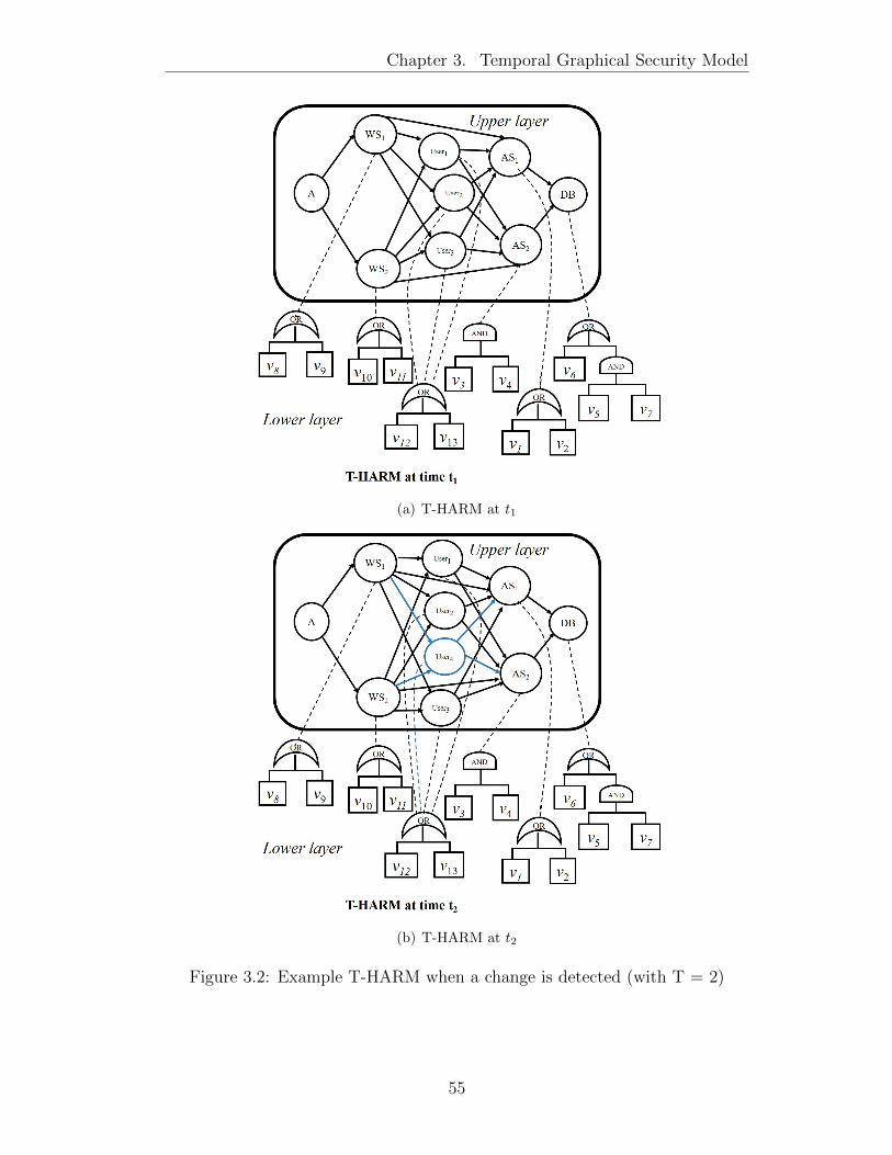
Chapter 3. Temporal Graphical Security Model
(a) T-HARM at t1
(b) T-HARM at t2
Figure 3.2: Example T-HARM when a change is detected (with T = 2)
55
Chapter 3. Temporal Graphical Security Model
3.5 Summary
The T-HARM and its formalisms are presented in this chapter. Also, a
systematic categorisation of possible security changes with respect to network
changes is presented along with its description and formalism. This chapter
developed the GSMs and introduced the security changes to be considered in
the remaining part of this thesis.
56
Chapter 4
Dynamic Security Assessments
Many security metrics for assessing cybersecurity have been developed and
formalised [34, 79, 114, 123, 126, 130, 136]. While these metrics remain useful in
assessing the security of networks, their effectiveness with respect to dynamic
changes in the network is still unclear. Therefore, it is important to investigate
how different security metrics are affected by changes in the network, in order
to identify which ones are suitable or not suitable for dynamic analysis.
First, this chapter describes composite security metrics for the security
analysis of networks. Second, it investigates the varying effects of security
metrics when changes are observed in the network. This investigation aims
to assist network/security administrators with the experimental results to
determine the security metric to use when a certain type of changes occurs
in a dynamic network. Based on the existing literature, this is the first work
to comprehensively investigate the effectiveness of existing security metrics for
the assessments of dynamic networks. The main contributions of this chapter
are summarised as follows:
� Proposed an approach to combining security metrics;
� Investigate the effect of the various network changes on the existing
security metrics over time;
� Conduct a comprehensive security analysis with various changes in T-
57
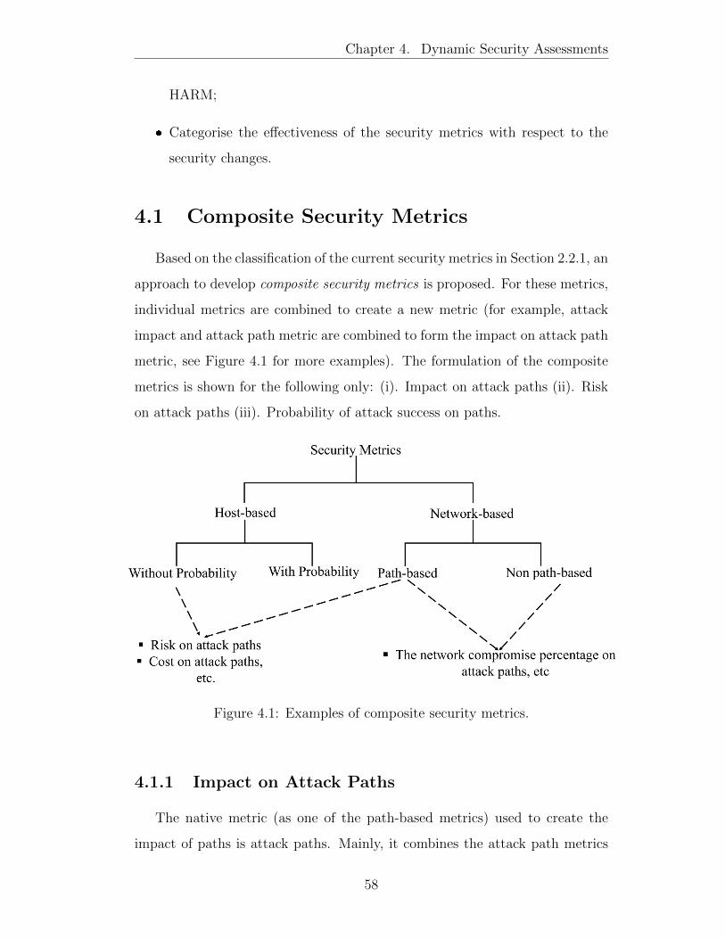
Chapter 4. Dynamic Security Assessments
HARM;
� Categorise the effectiveness of the security metrics with respect to the
security changes.
4.1 Composite Security Metrics
Based on the classification of the current security metrics in Section 2.2.1, an
approach to develop composite security metrics is proposed. For these metrics,
individual metrics are combined to create a new metric (for example, attack
impact and attack path metric are combined to form the impact on attack path
metric, see Figure 4.1 for more examples). The formulation of the composite
metrics is shown for the following only: (i). Impact on attack paths (ii). Risk
on attack paths (iii). Probability of attack success on paths.
Figure 4.1: Examples of composite security metrics.
4.1.1 Impact on Attack Paths
The native metric (as one of the path-based metrics) used to create the
impact of paths is attack paths. Mainly, it combines the attack path metrics
58
Chapter 4. Dynamic Security Assessments
with the impact of each host in the path. The Impact on Attack Paths is
defined as the cumulative quantitative measure of potential harm on an attack
path. Here, the vulnerability level metric is calculated by Equation (4.1), the
host attack impact is calculated by equation (4.2) and the attack-path level
metric is calculated by Equation (4.3). The network-level value AIMti is then
given by Equation (4.4).
aimbti=
∑
vti∈cti (bti )aimvti
, bti∈Btigti (bti )=AND
maxvti∈cti (bti )
aimvti, bti∈Bti
gti (bti )=OR
(4.1)
aimhti
= aimrootti(4.2)
aimapiti =
∑hti∈api
aimhti, api ∈ APnsti (4.3)
AIMti = maxapi∈APnsti
aimapiti (4.4)
The impact on path metric can reveal the impact of damage associated with
each attack path. A security administrator can use this metric to determine
which path to patch first. For instance, hosts in the path with the highest
impact value can be considered as the prioritised set of hosts to patch.
4.1.2 Risk on Attack Paths
The Risk on attack paths is defined as the expected value of the impact
on an attack path. It is computed as the summation of the product of the
probability of attack success prh and the amount of damage aimh h belonging
to an attack path ap. In the equation, the vulnerability level risk is calculated
by Equation (4.5), the host risk metric is calculated by Equation (4.6) and
the attack path level metric is calculated by Equation (4.7). The network-level
59

Chapter 4. Dynamic Security Assessments
value Rti is then given by Equation (4.8).
rbti =
∑
vti∈cti (bti )prvti × aimvti
, bti∈Btigti (bti )=AND
maxvti∈cti (bti )
prvti × aimvti, bti∈Bti
gti (bti )=OR
(4.5)
rhti = rrootti (4.6)
rapiti =∑
hti∈apiprhti × aim
hti, api ∈ APnsti (4.7)
Rti = maxapi∈APnsti
rapiti (4.8)
4.1.3 Probability of Attack Success on Paths
The probability of attack success on paths is developed by combining path
and probability of attack success. The probability of attack success on paths
represents the chances of an attacker successfully reaching the target through
an attack path. Equation 4.9 defines the vulnerability level attack success
probability, Equation (4.10) defines the host level attack success probability,
Equation (4.11) defines the attack path attack success probability. The
network-level value Prti is then given by Equation (4.12).
prbti =
∏
vti∈cti (bti )prvti ,
bti∈Btigti (bti )=AND
1−∏
vti∈cti (bti )(1− prvti ),
bti∈Btig(bti )=OR
(4.9)
prhti = prrootti (4.10)
prapiti =∏
hti∈apiprhti , api ∈ APnsti (4.11)
60

Chapter 4. Dynamic Security Assessments
Prti = maxapi∈APnsti
prapiti (4.12)
4.2 Evaluating the Effectiveness of Existing
Security Metrics for Dynamic Networks
This section investigates the effectiveness of the existing security metrics
for the analysis of dynamic networks. The metrics (and their formula) used in
this investigations are outlined in Section 4.2.1.
4.2.1 Security Metrics and their Computations
Eleven main security metrics from [33,79,102,126] are evaluated (in addition
to the composite metrics). The metrics and their formulas are shown in
Table 4.1. For each formula, the attribute time t is introduced so that it
can be used in the T-HARM.
Vulnerabilities are collected from a repository NVD [115]) which contains
vulnerabilities and their standardised severity score (in real networks, such
information is collected using scanners such as Nmap [120], OpenVAS [125],
etc). These scores are ranging from 0.0 to 10.0, with 10.0 being the most
severe level. The vulnerability impact sub score is used as the aimv and based
on the vulnerability CVSS BS [115], values are assigned to the prv and acv for
each of the vulnerabilities.
To evaluate the metrics, T-HARM is used to find all potential attack paths
over time. The potential attack paths ap are calculated in the upper layer of T-
HARM (the potential attack paths and entry point can change over time). The
host level metrics achti , rhti
, prhti , aimhti
and roahti are calculated from the lower
layer of T-HARM. The metrics NAPti , MoPLti , SDPLti , MAPLti , NMPLti
and SAPti [79] are calculated in the the upper layer of the T-HARM while the
metrics Rti , ACti , Prti , ROAti and PSSti are calculated using the host level
61
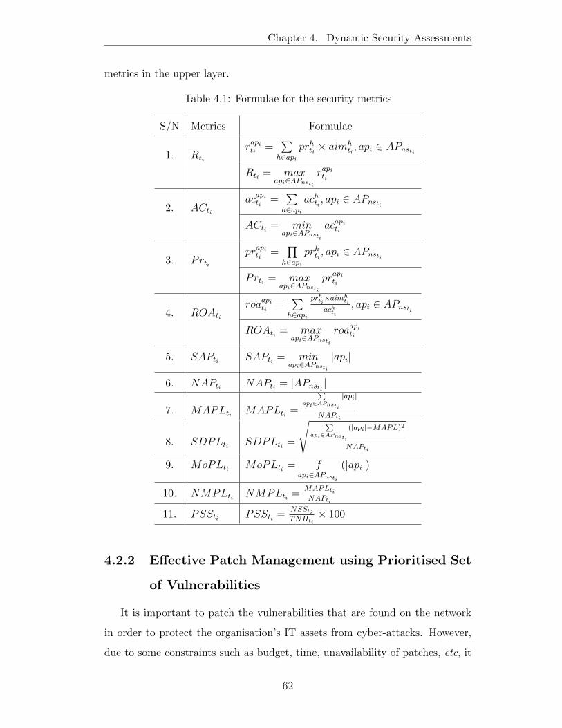
Chapter 4. Dynamic Security Assessments
metrics in the upper layer.
Table 4.1: Formulae for the security metrics
S/N Metrics Formulae
1. Rti
rapiti =∑h∈api
prhti × aimhti, api ∈ APnsti
Rti = maxapi∈APnsti
rapiti
2. ACtiacapiti =
∑h∈api
achti , api ∈ APnsti
ACti = minapi∈APnsti
acapiti
3. Prtiprapiti =
∏h∈api
prhti , api ∈ APnsti
Prti = maxapi∈APnsti
prapiti
4. ROAtiroaapiti =
∑h∈api
prhti×aimhtiachti
, api ∈ APnsti
ROAti = maxapi∈APnsti
roaapiti
5. SAPti SAPti = minapi∈APnsti
|api|
6. NAPti NAPti = |APnsti |
7. MAPLti MAPLti =
∑api∈APnsti
|api|
NAPti
8. SDPLti SDPLti =
√ ∑api∈APnsti
(|api|−MAPL)2
NAPti
9. MoPLti MoPLti = fapi∈APnsti
(|api|)
10. NMPLti NMPLti =MAPLtiNAPti
11. PSSti PSSti =NSStiTNHti
× 100
4.2.2 Effective Patch Management using Prioritised Set
of Vulnerabilities
It is important to patch the vulnerabilities that are found on the network
in order to protect the organisation’s IT assets from cyber-attacks. However,
due to some constraints such as budget, time, unavailability of patches, etc, it
62

Chapter 4. Dynamic Security Assessments
is sometimes infeasible to patch all the identified vulnerabilities [24]. Hence,
the approach called PSV [76] method is used to determine the set of critical
vulnerabilities to patch first for the network. A PSV is defined as a set of
vulnerabilities which are most important to enhance security. It is possible to
use the PSV method using a Top-Down, Bottom-Up or Hybrid approach to
manage the vulnerabilities found in the network system. Work [76] has the
complete detail of those approaches. The hybrid method is adapted for this
chapter, and the description is provided in Section 4.2.2.1.
4.2.2.1 PSV hybrid method
The hybrid method is used to rank vulnerabilities based on values calculated
from assigning weights to value of vulnerabilities and hosts, then combining
them to get a combined important measures value for each vulnerability. The
combined important measures value (CVv) for each vulnerability is calculated
by equation (4.13).
CVv = αNMhvname + (1− α)vmetric (4.13)
Where:
� vname is a vulnerability;
� NMhvname is the Network Centrality Measure value for a host h containing
the vulnerability vname;
� vmetric is the security metric for the vname.
� 0 ≤ α ≤ 1 is a weight value
� A weight value of α = 0.5 is reasonable selected and used. However,
this value can be adjusted such that the most important factor (e.g., the
vulnerability or the well connected host) is giving a higher weight value.
63
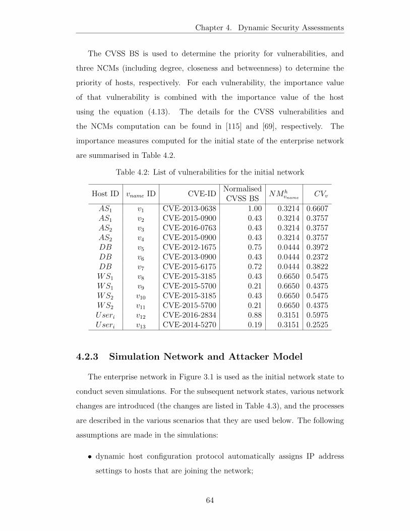
Chapter 4. Dynamic Security Assessments
The CVSS BS is used to determine the priority for vulnerabilities, and
three NCMs (including degree, closeness and betweenness) to determine the
priority of hosts, respectively. For each vulnerability, the importance value
of that vulnerability is combined with the importance value of the host
using the equation (4.13). The details for the CVSS vulnerabilities and
the NCMs computation can be found in [115] and [69], respectively. The
importance measures computed for the initial state of the enterprise network
are summarised in Table 4.2.
Table 4.2: List of vulnerabilities for the initial network
Host ID vname ID CVE-IDNormalisedCVSS BS
NMhvname CVv
AS1 v1 CVE-2013-0638 1.00 0.3214 0.6607AS1 v2 CVE-2015-0900 0.43 0.3214 0.3757AS2 v3 CVE-2016-0763 0.43 0.3214 0.3757AS2 v4 CVE-2015-0900 0.43 0.3214 0.3757DB v5 CVE-2012-1675 0.75 0.0444 0.3972DB v6 CVE-2013-0900 0.43 0.0444 0.2372DB v7 CVE-2015-6175 0.72 0.0444 0.3822WS1 v8 CVE-2015-3185 0.43 0.6650 0.5475WS1 v9 CVE-2015-5700 0.21 0.6650 0.4375WS2 v10 CVE-2015-3185 0.43 0.6650 0.5475WS2 v11 CVE-2015-5700 0.21 0.6650 0.4375Useri v12 CVE-2016-2834 0.88 0.3151 0.5975Useri v13 CVE-2014-5270 0.19 0.3151 0.2525
4.2.3 Simulation Network and Attacker Model
The enterprise network in Figure 3.1 is used as the initial network state to
conduct seven simulations. For the subsequent network states, various network
changes are introduced (the changes are listed in Table 4.3), and the processes
are described in the various scenarios that they are used below. The following
assumptions are made in the simulations:
� dynamic host configuration protocol automatically assigns IP address
settings to hosts that are joining the network;
64

Chapter 4. Dynamic Security Assessments
� users can install software on this hosts, and the software may have one
or more vulnerability;
� Among other activities, the administrators can perform tasks such as
disabling vulnerable hosts, software, etc., and changing of firewall rules;
� there is always at least a type of server that is up and running at any
time t in order to guarantee the access of client to the DB (for example,
it is ensured that only one of the two web servers (WS1 and WS2) is
disconnected or removed from the network per time).
� the network states are captured when changes are observed in the network
(but in a few scenarios, a fixed change in t between different network
states is used).
T-HARM is constructed for the dynamic network using the inputs above
and the attacker model specified in Section 3.2.2. Then, several security metrics
are calculated in the various scenarios. The simulations focused on investigating
the varying effects of security metrics when changes are observed in the network
for the following scenarios (such that all the network changes specified in
Table 3.2 are captured and analysed): (1) Addition of software vulnerabilities
(Section 4.3.1), (2) Addition of new hosts (hosts having vulnerabilities) (Section
4.3.2), (3) Software Update (e.g., patching of vulnerabilities) (Section 4.3.3),
(4) Disabling application software (Section 4.3.4), (5) Installation of new
application software (Section 4.3.5), (6) Removal of existing hosts (Section
4.3.6), and (7) Change of firewall rules (Section 4.3.7).
Simulation results: Line graphs are used to present the simulation results.
In the graphs, the change of time t is presented on the horizontal axis and
the normalised metric value on the vertical axis. All the metrics values are
normalised (i.e., ranging from 0.0 to 1.0).
65

Chapter 4. Dynamic Security Assessments
4.3 Scenario Descriptions and Results
Experimental analysis via simulations is conducted using the T-HARM for
the network changes described in Table 3.2. To achieve this, the network
changes with respect to security changes in Table 4.3 are mapped and used for
the simulations, accordingly.
Table 4.3: Simulations: security changes with respect to network changes
Changes in security Causes of configurations changeRelated
subsection(s)
Addition of vulnerabilities
(1) installation of software 4.3.5
(2) software turned on or enabled 4.3.5
(3) addition of new hosts 4.3.2
(4) discovery of vulnerabilities 4.3.1
Removal of vulnerabilities
(1) update of software 4.3.3
(2) uninstallation of software 4.3.4
(3) software turned off or disabled 4.3.4
(4) removal of hosts 4.3.6
Addition of nodes
(1) addition of hosts 4.3.2
(2) installation of software 4.3.5
(3) software turned on or enabled 4.3.5
(4) host turned on 4.3.2
Removal of nodes
(1) removal of hosts 4.3.6
(2) uninstallation of software 4.3.4, 4.3.3
(3) update of software 4.3.3
(4) software turned off or disabled 4.3.4
Addition of edges
(1) addition of host 4.3.2
(2) host turn on 4.3.2
(3) connection of host 4.3.7, 4.3.2
(4) firewall rules changed 4.3.7
(5) installation of software 4.3.5
Removal of edges
(1) removal of host 4.3.6
(2) host turned off or failed 4.3.6
(3) disconnection of host 4.3.7
(4) firewall rule changed 4.3.7
(5) software turned off or disabled 4.3.4
66
Chapter 4. Dynamic Security Assessments
4.3.1 Scenario I: Addition of Vulnerability
Software often has vulnerabilities and these can be discovered (or be
emerging) over time [105]. In consequence, the security of hosts in a network
system is continuously affected. In this regard, the vulnerabilities of the
network states are captured at different time, and it is assumed that the
vulnerabilities are not patched between the changes in states. This section aims
to capture and investigate how security metrics change when vulnerabilities are
discovered over time, and so, it is assumed that the software vendors did not
release the patches for the vulnerabilities within those time. Besides, many
systems are left unpatched for months and sometimes, even years [147]. In
some cases, unknown vulnerabilities (e.g., zero-day vulnerabilities [58]) are
impossible to patch. Consequently, this section explores how the existing
security metrics change when vulnerabilities are found (announced) and left
un-patched (a more detailed description of this scenario is given in [20]).
To simulate this, vulnerability data are collected for 12 months (i.e., from
April 2015 to March 2016) from the NVD (i.e., for both the OSes and
applications summarised in Table 3.1). After that, the collected vulnerabilities
are extracted into their respective time of discovery, which is summarised in
Table 4.4 and then further, they are used as input (they are used sequentially)
into T-HARM (this captures the emergence of the vulnerabilities over time).
In this case, it is assumed that the hosts and reachability are not changing.
The T-HARM with time window T = 13 is used for the analysis and each time
ti is representing a month.
67
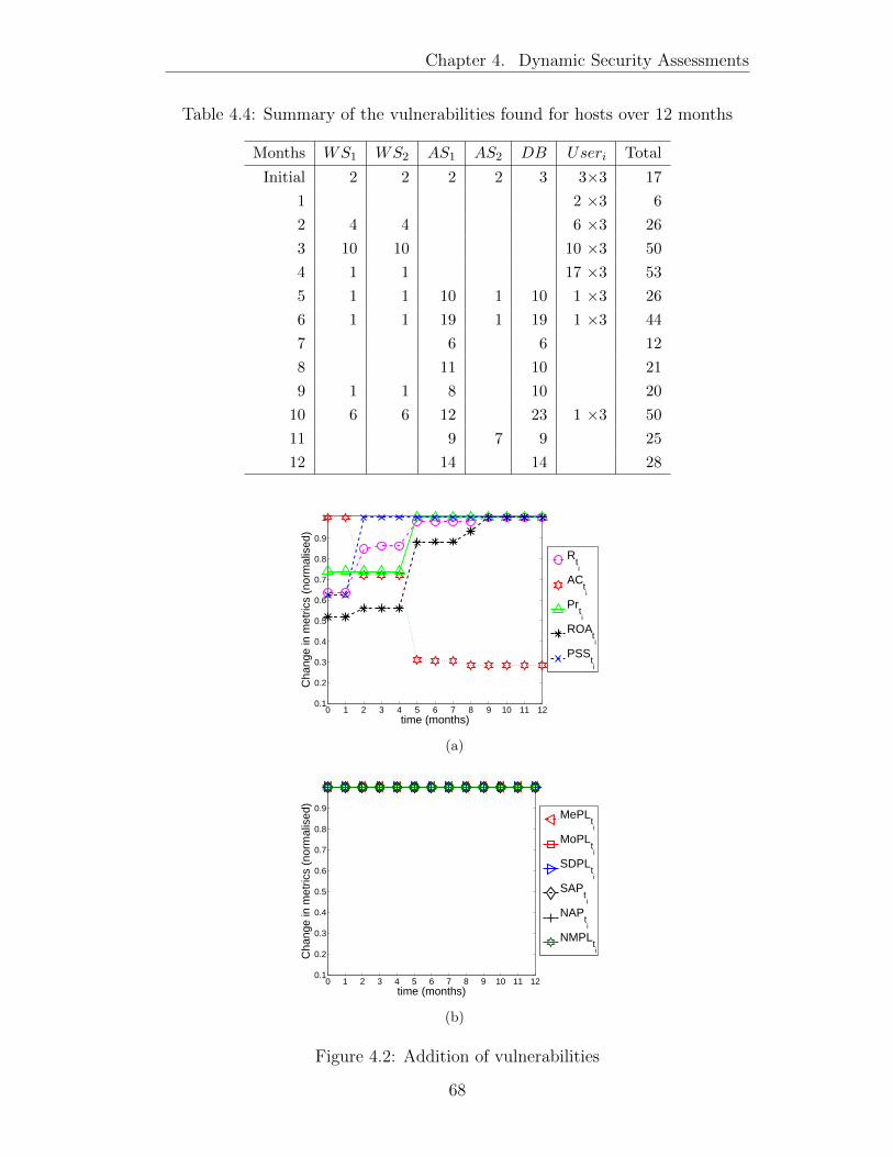
Chapter 4. Dynamic Security Assessments
Table 4.4: Summary of the vulnerabilities found for hosts over 12 months
Months WS1 WS2 AS1 AS2 DB Useri Total
Initial 2 2 2 2 3 3×3 17
1 2 ×3 6
2 4 4 6 ×3 26
3 10 10 10 ×3 50
4 1 1 17 ×3 53
5 1 1 10 1 10 1 ×3 26
6 1 1 19 1 19 1 ×3 44
7 6 6 12
8 11 10 21
9 1 1 8 10 20
10 6 6 12 23 1 ×3 50
11 9 7 9 25
12 14 14 28
0 1 2 3 4 5 6 7 8 9 10 11 120.1
0.2
0.3
0.4
0.5
0.6
0.7
0.8
0.9
1
time (months)
Cha
nge
in m
etric
s (n
orm
alis
ed)
Rti
ACti
Prti
ROAti
PSSti
(a)
0 1 2 3 4 5 6 7 8 9 10 11 120.1
0.2
0.3
0.4
0.5
0.6
0.7
0.8
0.9
1
time (months)
Cha
nge
in m
etric
s (n
orm
alis
ed)
MePLti
MoPLti
SDPLti
SAPti
NAPti
NMPLti
(b)
Figure 4.2: Addition of vulnerabilities
68

Chapter 4. Dynamic Security Assessments
Figure 4.2 shows the result of the discovery of vulnerability for the different
months. The result show that the metrics Rt2 , ACt2 ROAt2 and ROAt2 (i.e.,
t = 2 ) significantly change at t2. The reason is, at that point the severity of
vulnerabilities on attack paths to the target host has started to become high
for each host (which happens as the result of the increase in the number of
new vulnerabilities) compared to the earlier network state, thus causing the
sharp change in the metric value. Similarly, Rt5 , ACt5 , Prt5 and ROAt5 change
significantly and this is for the same reason. On the other hand, the Rt9 , ACt9 ,
ROAt9 , ACt5 and PSSt2 become static at these points because the host level
values (i.e., the risk severity value) reach the maximum value (i.e., 10.00 for
each of the hosts) and consequently, the network-level security metrics do not
change. On the other hand, the other security metrics (i.e., MePLti , MoPLti ,
SDPLti , SAPti , NAPti and NMPLti) do not change for all the time as all
the hosts in the network regularly have at least one exploitable vulnerability.
Hence, it does not change the reachability in the upper layer (i.e., attack paths
to the target host) for the entire time window. So, MePLti , MoPLti , SDPLti ,
SAPti , NAPti and NMPLti do not change for all the time; Rti , ACti , Prti , ROAti
and PSSti continue to deteriorate in their security value. This demonstrates
that Rti , ACti , Prti , ROAti and PSSti can satisfactory reflect the emergence of
vulnerabilities over time.
In summary, the results of this scenario showed that Rti , ACti , Prti ,
ROAti and PSSti change in their values accordingly, however as the number
of vulnerabilities becomes large for each host, their values become static.
Contrarily, the MePLti , MoPLti , SDPLti , SAPti , NAPti and NMPLti remain
static for all the time.
4.3.2 Scenario II: Addition of Hosts
Modern networks are flexible, and as a result, they allow components to
be added to the network at various times. Moreover, organisations sometimes
increase the size of networks to meet current demands (e.g., by adding new
69
Chapter 4. Dynamic Security Assessments
devices). However, the addition of components can affect the security posture
of networks [19]. Hence, this section investigates the effect of the addition of
hosts on the existing security metrics.
Here, the addition of hosts to the example network in Figure 3.1 is considered.
In the simulation, all the hosts are up and running for all the time. Also,
the vulnerabilities listed in Table 4.4 are used for the simulation. Further,
the network traffic (for WSs, DB, ASs, and users’ workstations) remain as
described in Section 3.2.1. However, only the addition of users’ workstations is
considered. Here, the number of workstations is increased by 20% each time.
The results are shown in Figure 4.3.
70

Chapter 4. Dynamic Security Assessments
0 2 4 6 8 10 12 14 16 18 20 220.5
0.6
0.7
0.8
0.9
1
Number of hosts
Cha
nge
in m
etric
(no
rmal
ised
)
Rti
ACti
Prti
ROAti
PSSti
(a)
0 2 4 6 8 10 12 14 16 18 20 220
0.1
0.2
0.3
0.4
0.5
0.6
0.7
0.8
0.9
1
Number of hosts
Cha
nge
in m
etric
(no
rmal
ised
)
MePLti
MoPLti
SDPLti
SAPti
NAPti
NMPLti
(b)
Figure 4.3: Change with respect to addition of hosts
From the result shown in Figure 4.3, the addition of new hosts to the
network does not change SAPti , MoPLti ACti and Prti compared to the initial
network. However, the metric at R3 (i.e., at the number of host = 6) and ROAt3
and Rt3 and ACt7 (i.e., at the number of host = 14) increase significantly from
the previous security state. It is at these two points (and time) that servers are
added to the network (i.e., and WS and AS, respectively) thus causing a change
71
Chapter 4. Dynamic Security Assessments
in the metrics value. On the other hand, PSSti , MePLti , MoPLti , SDPLti ,
NAPti and NMPLti change progressive for all the time which indicates the
decrease in security. Similarly, MePLt3 , MoPLt3 , SDPLt3 , NAPt3 and NMPLt3
indicate significant (sharp) change for the addition of a WS server. Also, it
is observed that the SAPti does not change because the minimum number of
hosts needed along the attack path for an attacker to reach the target remains
the same as the initial network configuration. Similarly, the MoPLti does not
change because the length of attack path that appears the most frequently (for
each network state) remains the same as well.
In summary, the results shows that the PSSti , MePLti , MoPLti , SDPLti ,
NAPti and NMPLti change significantly. Conversely, Rti , ACti and ROAti only
show limited change and the SAPti and Prti do not change for all the time.
4.3.3 Scenario III: Software Update
Software vendors tend to actively release patches for their software products
and then leave it to the customers to decide whether to apply those software
corrections or not [42]. The implementation of these updates can remove one
or more vulnerabilities from the software and hence, for a networked system
(where a cyber-attacker uses this defect to bypass security measures) the
removal of these set of vulnerabilities changes the security posture, and the
network will need to be re-assessed to determine the security. At this point, it
is of interest to investigate what security metrics are changing when software
is updated over time.
Here, the following assumptions are made: (i) that patches are regularly
performed once per month and (ii) that all patches are tested first in a
pre-production environment before applying to the network devices (hence,
there is no failure during patches). Also, the enterprise network vulnerability
information is known for twelve months (as they are collected already from
NVD which are shown in scenario 4.3.1). Additionally, since the organisation
cannot afford to patch all the vulnerabilities due to cost, time, unavailability
72
Chapter 4. Dynamic Security Assessments
of patches and other security policies, the risk-based PSV using hybrid method
is used (from Section 4.2.2.1). Simulations are performed using different PSV
values (i.e., 30%, 50% and 70%), however only one PSV value for each time
window is used. the results are plotted in Figure 4.4. In particular, the result
for the PSV at 30%, 50% and 70% is plotted in Figure 4.4(a) and 4.4(b), 4.4(c)
and 4.4(d), 4.4(e) and 4.4(f), respectively.
73
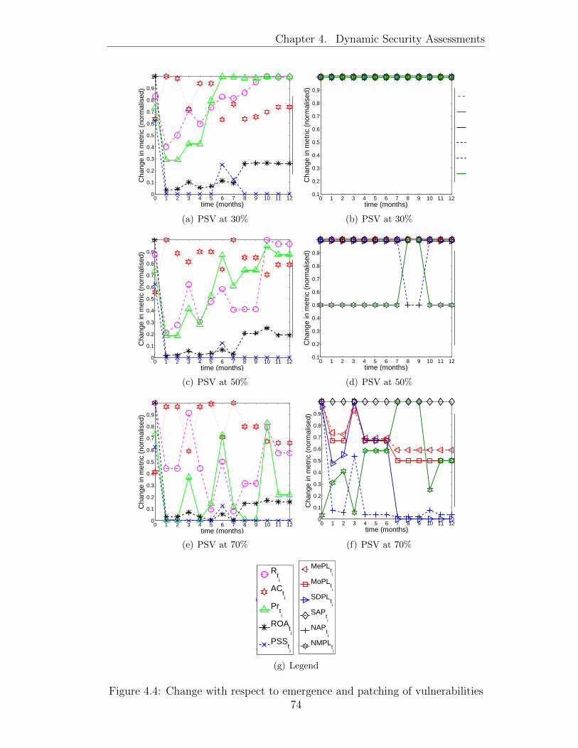
Chapter 4. Dynamic Security Assessments
0 1 2 3 4 5 6 7 8 9 10 11 120
0.1
0.2
0.3
0.4
0.5
0.6
0.7
0.8
0.9
1
time (months)
Cha
nge
in m
etric
(no
rmal
ised
)
Rti
ACti
Prti
ROAti
PSSti
(a) PSV at 30%
0 1 2 3 4 5 6 7 8 9 10 11 120.1
0.2
0.3
0.4
0.5
0.6
0.7
0.8
0.9
1
time (months)
Cha
nge
in m
etric
(no
rmal
ised
)
MePLti
MoPLti
SDPLti
SAPti
NAPti
NMPLti
(b) PSV at 30%
0 1 2 3 4 5 6 7 8 9 10 11 120
0.1
0.2
0.3
0.4
0.5
0.6
0.7
0.8
0.9
1
time (months)
Cha
nge
in m
etric
(no
rmal
ised
)
Rti
ACti
Prti
ROAti
PSSti
(c) PSV at 50%
0 1 2 3 4 5 6 7 8 9 10 11 120.1
0.2
0.3
0.4
0.5
0.6
0.7
0.8
0.9
1
time (months)
Cha
nge
in m
etric
(no
rmal
ised
)
MePLti
MoPLti
SDPLti
SAPti
NAPti
NMPLti
(d) PSV at 50%
0 1 2 3 4 5 6 7 8 9 10 11 120
0.1
0.2
0.3
0.4
0.5
0.6
0.7
0.8
0.9
1
time (months)
Cha
nge
in m
etric
(no
rmal
ised
)
Rti
ACti
Prti
ROAti
PSSti
(e) PSV at 70%
0 1 2 3 4 5 6 7 8 9 10 11 120
0.1
0.2
0.3
0.4
0.5
0.6
0.7
0.8
0.9
1
time (months)
Cha
nge
in m
etric
(no
rmal
ised
)
MePLti
MoPLti
SDPLti
SAPti
NAPti
NMPLti
(f) PSV at 70%
0 1 2 3 4 5 6 7 8 9 10 11 120
0.1
0.2
0.3
0.4
0.5
0.6
0.7
0.8
0.9
1
time (months)
Cha
nge
in m
etric
(no
rmal
ised
)
Rti
ACti
Prti
ROAti
PSSti
0 1 2 3 4 5 6 7 8 9 10 11 120
0.1
0.2
0.3
0.4
0.5
0.6
0.7
0.8
0.9
1
time (months)
Cha
nge
in m
etric
(no
rmal
ised
)
MePLti
MoPLti
SDPLti
SAPti
NAPti
NMPLti
(g) Legend
Figure 4.4: Change with respect to emergence and patching of vulnerabilities74
Chapter 4. Dynamic Security Assessments
In Figure 4.4(a), it is observed that Rti , ACti , Prti , ROAti and PSSti change
accordingly when vulnerabilities are patched. It is also observed that even when
vulnerabilities are patched per month, the security keeps deteriorating over
time for the reason that the PSV value used is low compared to the number
of vulnerabilities found at each time t. However, the result shows that the
regular patching of the vulnerabilities keep the metric PSSti very low (since
critical vulnerabilities are always patched first). Although, at PSSt6 the value
increases because most of the vulnerabilities discovered at this point have high
CVSS values (i.e., critical vulnerabilities).
On the other hand, in Figure 4.4(b) SAPti , NAPti , MAPLti , MoPLti , SDPLti
and NMPLti do not change for most of the time. Here, it shows that
this happened because there is always at least one exploitable vulnerability
remaining on each host in the network and hence, the attack paths in the
upper layer do not change. Nevertheless, as the PSV value is increased to
50% (as shown in Figure 4.4(c) and 4.4(d)), it result showed that all the
metrics in Figure 4.4(c) change continuously while in Figure 4.4(d), only NAPti
and NMPLti that showed a small change (i.e., between month 8 to month 9)
however, it became static again during the remaining period. In Figure 4.4(d),
the regular patching of vulnerabilities at PSV = 50% was able to remove all the
vulnerabilities found on some hosts at month 8 and month 9 (which changes
some possible attack paths). Hence the change in NAPt8 , NMPLt8 , NAPt9
and NMPLt9 compared to the initial network state. Furthermore, when the
PSV value is increased to 70% (in Figure 4.4(e) and 4.4(f)), all metrics show
a significant change in their values for all the months except the SAPti . The
SAPti do not change because the minimum number of hosts along the attack
path for the attacker to reach the target remain the same as the initial network
configuration. This implies that when the values of the PSV are high, all
the security metrics will show a significant change in their values (except the
SAPti).
75
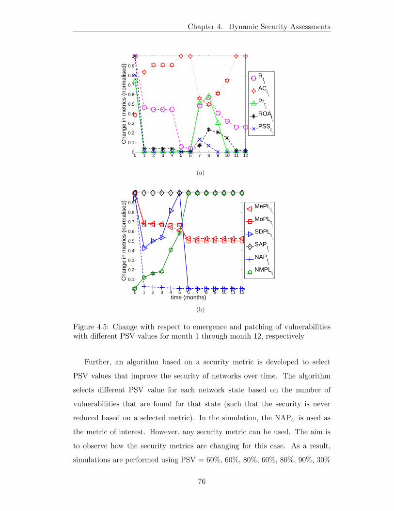
Chapter 4. Dynamic Security Assessments
0 1 2 3 4 5 6 7 8 9 10 11 120
0.1
0.2
0.3
0.4
0.5
0.6
0.7
0.8
0.9
1
Cha
nge
in m
etric
s (n
orm
alis
ed)
Rti
ACti
Prti
ROAti
PSSti
(a)
0 1 2 3 4 5 6 7 8 9 10 11 120
0.1
0.2
0.3
0.4
0.5
0.6
0.7
0.8
0.9
1
time (months)
Cha
nge
in m
etric
s (n
orm
alis
ed)
MePLti
MoPLti
SDPLti
SAPti
NAPti
NMPLti
(b)
Figure 4.5: Change with respect to emergence and patching of vulnerabilitieswith different PSV values for month 1 through month 12, respectively
Further, an algorithm based on a security metric is developed to select
PSV values that improve the security of networks over time. The algorithm
selects different PSV value for each network state based on the number of
vulnerabilities that are found for that state (such that the security is never
reduced based on a selected metric). In the simulation, the NAPti is used as
the metric of interest. However, any security metric can be used. The aim is
to observe how the security metrics are changing for this case. As a result,
simulations are performed using PSV = 60%, 60%, 80%, 60%, 80%, 90%, 30%
76
Chapter 4. Dynamic Security Assessments
, 30%, 70%, 90%, 80% and 80% for month 1 through month 12, respectively
(the algorithm (in Algorithm 1) selected these values). The following notations
are used in the algorithm:
� PSV : prioritise set of vulnerabilities (calculated in Section 4.2.2.1)
� spsvti : a PSV value for sti
� SW : set of PSV value for a time window (spsvti ∈ PV )
� smetricti: a calculated security metric for sti
The Algorithm 1 takes a copy of the simulation network to calculate the
PSV value for each network state. First, the first network state is used as the
initial network (line 2). For each network states (line 3), the metric NAP is
calculated for each of the sti (line 4 and 5). Further, the appropriate PSV to
use is calculated (line 7 and 8 based on Section 4.2.2.1). In line 8 and 9, the
PSV calculated are then patched. For each of the vulnerability (v) patched, the
metric (sNAPti) is calculated (line 10) until the calculated sNAPti+1
is less than the
previous network state (sNAPti−1) from S (line 11 and 12) in the set of solutions
in SW .
The results are plotted in Figure 4.5. From the results, the NAPti , MAPLti ,
MoPLti , SDPLti and NMPLti change progressively and until ‘month 6’ when
there is only an attack path to reach the target host. This is because a ‘forever
day’ vulnerability is used, which is not removed by software update hence, there
is always an attack path to reach the target host. Additionally, the results show
that the SAPti remains static for all the time (this is because the minimum
number of hosts along the attack path for the attacker to reach the target
remain the same with the initial network.). On the other hand, the Rti , ACti ,
Prti , ROAti , SDPLti and PSSti change progressively as the number of paths are
progressively reduced over time. However, at Rt7 , ACt7 , Prt7 , ROAt7 and PSSt7 ,
the metric start deteriorating but later improve again. The manual analysis
performed revealed that even when there is only an attack path to reach the
77
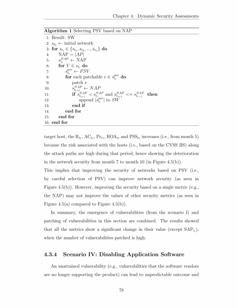
Chapter 4. Dynamic Security Assessments
Algorithm 1 Selecting PSV based on NAP
1: Result: SW2: st0 ← initial network3: for sti ∈ {st1 , st2 , ..., stn} do4: NAP = |AP |5: sNAPti
← NAP6: for V ∈ sti do7: spsvti ← PSV8: for each patchable v ∈ spsvti do9: patch v
10: sNAPti+1← NAP
11: if sNAPti+1< sNAPti
and sNAPti+1<= sNAPti−1
then12: append |spsvti | to SW13: end if14: end for15: end for16: end for
target host, the Rt7 , ACt7 , Prt7 , ROAt7 and PSSt7 increases (i.e., from month 5)
because the risk associated with the hosts (i.e., based on the CVSS BS) along
the attack paths are high during that period, hence showing the deterioration
in the network security from month 7 to month 10 (in Figure 4.5(b)).
This implies that improving the security of networks based on PSV (i.e.,
by careful selection of PSV) can improve network security (as seen in
Figure 4.5(b)). However, improving the security based on a single metric (e.g.,
the NAP) may not improve the values of other security metrics (as seen in
Figure 4.5(a) compared to Figure 4.5(b)).
In summary, the emergence of vulnerabilities (from the scenario I) and
patching of vulnerabilities in this section are combined. The results showed
that all the metrics show a significant change in their value (except SAPti),
when the number of vulnerabilities patched is high.
4.3.4 Scenario IV: Disabling Application Software
An unattained vulnerability (e.g., vulnerabilities that the software vendors
are no longer supporting the product) can lead to unpredictable outcome and
78
Chapter 4. Dynamic Security Assessments
as such, security administrators need to mitigate the impact of the unattained
vulnerabilities by disabling or turning off the service that is associated to the
vulnerability [105] in order to avoid exposure to different type of cyber-attack.
In this section, the action of how the turning off of a vulnerable application
on a host will change the various security metrics in a network system is
investigated. The system settings and configurations from section 3.2 are used
for this simulation. It is assumed that there is only one vulnerable application
that has no security patch per time. Hence, only one application per time is
disabled in the simulations. However, the application on the DB is not disabled,
and this is to ensure users access to the database. The results are shown in
Figure 4.6.
79
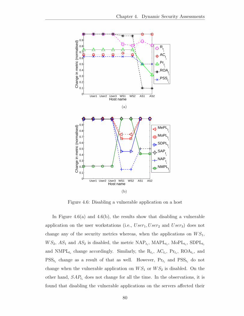
Chapter 4. Dynamic Security Assessments
User1 User2 User3 WS1 WS2 AS1 AS20
0.1
0.2
0.3
0.4
0.5
0.6
0.7
0.8
0.9
1
Host name
Cha
nge
in m
etric
(no
rmal
ised
)
Rti
ACti
Prti
ROAti
PSSti
(a)
User1 User2 User3 WS1 WS2 AS1 AS20
0.1
0.2
0.3
0.4
0.5
0.6
0.7
0.8
0.9
1
Host name
Cha
nge
in m
etric
(no
rmal
ised
)
MePLti
MoPLti
SDPLti
SAPti
NAPti
NMPLti
(b)
Figure 4.6: Disabling a vulnerable application on a host
In Figure 4.6(a) and 4.6(b), the results show that disabling a vulnerable
application on the user workstations (i.e., User1, User2 and User3) does not
change any of the security metrics whereas, when the applications on WS1,
WS2, AS1 and AS2 is disabled, the metric NAPti , MAPLti , MoPLti , SDPLti
and NMPLti change accordingly. Similarly, the Rti , ACti , Prti , ROAti , and
PSSti change as a result of that as well. However, Prti and PSSti do not
change when the vulnerable application on WS1 or WS2 is disabled. On the
other hand, SAPti does not change for all the time. In the observations, it is
found that disabling the vulnerable applications on the servers affected their
80
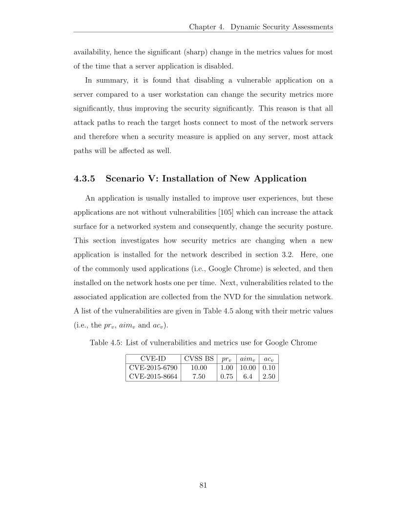
Chapter 4. Dynamic Security Assessments
availability, hence the significant (sharp) change in the metrics values for most
of the time that a server application is disabled.
In summary, it is found that disabling a vulnerable application on a
server compared to a user workstation can change the security metrics more
significantly, thus improving the security significantly. This reason is that all
attack paths to reach the target hosts connect to most of the network servers
and therefore when a security measure is applied on any server, most attack
paths will be affected as well.
4.3.5 Scenario V: Installation of New Application
An application is usually installed to improve user experiences, but these
applications are not without vulnerabilities [105] which can increase the attack
surface for a networked system and consequently, change the security posture.
This section investigates how security metrics are changing when a new
application is installed for the network described in section 3.2. Here, one
of the commonly used applications (i.e., Google Chrome) is selected, and then
installed on the network hosts one per time. Next, vulnerabilities related to the
associated application are collected from the NVD for the simulation network.
A list of the vulnerabilities are given in Table 4.5 along with their metric values
(i.e., the prv, aimv and acv).
Table 4.5: List of vulnerabilities and metrics use for Google Chrome
CVE-ID CVSS BS prv aimv acvCVE-2015-6790 10.00 1.00 10.00 0.10CVE-2015-8664 7.50 0.75 6.4 2.50
81

Chapter 4. Dynamic Security Assessments
AS2 DB3 User1 User2 User3 WS1 WS2 AS10
0.1
0.2
0.3
0.4
0.5
0.6
0.7
0.8
0.9
1
Host name
Cha
nge
in m
etric
(no
rmal
ised
)
Rti
ACti
Prti
ROAti
PSSti
AS2 DB3 User1 User2 User3 WS1 WS2 AS10
0.1
0.2
0.3
0.4
0.5
0.6
0.7
0.8
0.9
1
Host name
Cha
nge
in m
etric
(no
rmal
ised
)
MePLti
MoPLti
SDPLti
SAPti
NAPti
NMPLti
Figure 4.7: Installing an application on a host
The results are plotted in Figure 4.7. It is observed that the metrics -
Rti , ACti , ROAti and PSSti deteriorate in their values for each time that
a new application is installed on a host (this is because the installation of
the application increases the host’s risk value). Contrarily, MePLti , MoPLti ,
SDPLti , SAPti , NAPti and NMPLti do not change for all the time for the reason
that all the hosts in the network are regularly having other vulnerabilities.
Consequently, the attack paths to the target host do not change for the entire
time that a new application is installed. From the results of the simulations,
it is found that installing another vulnerability application on the DB affects
the Rti , ACti , ROAti , Prti and PSSti significantly (the security decrease a lot)
compared to any other hosts found in the network (with a high chance for
82

Chapter 4. Dynamic Security Assessments
the attacker to attack the target hosts). Similarly, the ACti reduces when an
application is installed on WS1 and WS2 demonstrating that a less effort is
required by the attacker to reach the target hosts.
The results in this section showed that the installation of new application on
a host does not change MePLti , MoPLti , SDPLti , SAPti , NAPti and NMPLti .
The reason is that there is already an exploitable vulnerability on each of the
network hosts (in the upper layer) and thus, all the possible attack paths to
reach the target host remain the same compared to the earlier network state.
This is consistent for all the scenarios in which this sets of metrics do not
change.
In summary, the results show that the MePLti , MoPLti , SDPLti , SAPti ,
NAPti and NMPLt do not change while the others change appropriately with
respect to the installation of a new application.
4.3.6 Scenario VI: Removal of Hosts
Modern network components can be removed or disconnected for many
reasons (e.g., OS failure, hardware failure, system upgrade, user, etc) and as a
result, the security posture of the network change. In this scenario, a simulation
is performed to investigate how the security changes with the removal of hosts.
In particular, an incremental removal of the host is considered over time.
However, in the simulation, it is ensured that there is always at least one
of each type of servers active (i.e., up and running) for all the time t in order
to guarantee the access of a client to the DB. The network in Figure 3.1 is used
with an addition of 20 more user workstations.
83

Chapter 4. Dynamic Security Assessments
0 2 4 6 8 10 12 14 16 18 20 220
0.1
0.2
0.3
0.4
0.5
0.6
0.7
0.8
0.9
1
Number of hosts
Cha
nge
in m
etric
(no
rmal
ised
)
Rti
ACti
Prti
ROAti
PSSti
(a)
0 2 4 6 8 10 12 14 16 18 20 220
0.1
0.2
0.3
0.4
0.5
0.6
0.7
0.8
0.9
1
Number of hosts
Cha
nge
in m
etric
(no
rmal
ised
)
MePLti
MoPLti
SDPLti
SAPti
NAPti
NMPLti
(b)
Figure 4.8: Change with respect to removal of hosts
The result for the metrics are plotted and shown in Figure 4.8. In particular,
Rti , ACti , ROAti , Prti and PSSti are plotted in Figure 4.8(a) and the results of
MePLti , MoPLti , SDPLti , SAPti , NAPti and NMPLti in Figure 4.8(b). From
the results, it is observed that the metrics in Figure 4.8(b) change frequently as
hosts are removed from the network (showing improvement in security) but the
SAPti does not change. In Figure 4.8(a), PSSti change continuously as hosts
are removed. Conversely, Rti , ROAti and Prti change significantly only when
the total number of hosts removed is 10. At this point, it is observed that this
is because a server (AS1) which connects most of the hosts to the target host
84
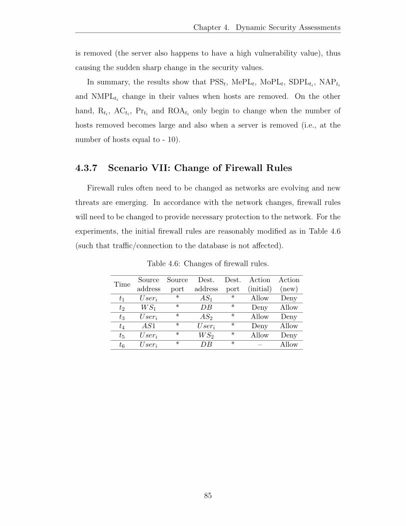
Chapter 4. Dynamic Security Assessments
is removed (the server also happens to have a high vulnerability value), thus
causing the sudden sharp change in the security values.
In summary, the results show that PSSt, MePLt, MoPLt, SDPLti , NAPti
and NMPLti change in their values when hosts are removed. On the other
hand, Rti , ACti , Prti and ROAti only begin to change when the number of
hosts removed becomes large and also when a server is removed (i.e., at the
number of hosts equal to - 10).
4.3.7 Scenario VII: Change of Firewall Rules
Firewall rules often need to be changed as networks are evolving and new
threats are emerging. In accordance with the network changes, firewall rules
will need to be changed to provide necessary protection to the network. For the
experiments, the initial firewall rules are reasonably modified as in Table 4.6
(such that traffic/connection to the database is not affected).
Table 4.6: Changes of firewall rules.
TimeSourceaddress
Sourceport
Dest.address
Dest.port
Action(initial)
Action(new)
t1 Useri * AS1 * Allow Deny
t2 WS1 * DB * Deny Allow
t3 Useri * AS2 * Allow Deny
t4 AS1 * Useri * Deny Allow
t5 Useri * WS2 * Allow Deny
t6 Useri * DB * – Allow
85
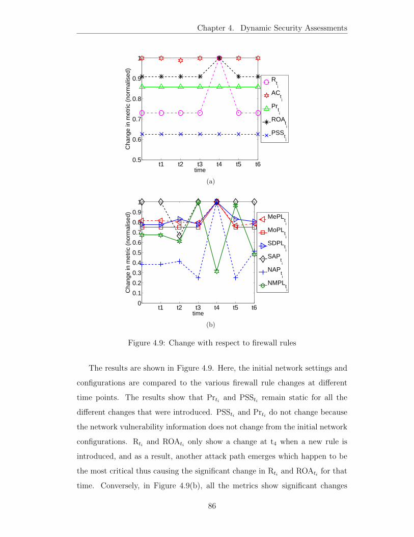
Chapter 4. Dynamic Security Assessments
t1 t2 t3 t4 t5 t60.5
0.6
0.7
0.8
0.9
1
time
Cha
nge
in m
etric
(no
rmal
ised
)
Rti
ACti
Prti
ROAti
PSSti
(a)
t1 t2 t3 t4 t5 t60
0.1
0.2
0.3
0.4
0.5
0.6
0.7
0.8
0.9
1
time
Cha
nge
in m
etric
(no
rmal
ised
)
MePLti
MoPLti
SDPLti
SAPti
NAPti
NMPLti
(b)
Figure 4.9: Change with respect to firewall rules
The results are shown in Figure 4.9. Here, the initial network settings and
configurations are compared to the various firewall rule changes at different
time points. The results show that Prti and PSSti remain static for all the
different changes that were introduced. PSSti and Prti do not change because
the network vulnerability information does not change from the initial network
configurations. Rti and ROAti only show a change at t4 when a new rule is
introduced, and as a result, another attack path emerges which happen to be
the most critical thus causing the significant change in Rti and ROAti for that
time. Conversely, in Figure 4.9(b), all the metrics show significant changes
86
Chapter 4. Dynamic Security Assessments
with respect to the different security changes accordingly except the SAP.
In summary, the MePLti , MoPLti , SDPLti , SAPti , NAPti and NMPLti change
accordingly for this network change. Rti , ACti and ROAti only show small
change and PSSti and Prti do not change for the entire time window.
4.3.8 Summary of the Results
The enterprise network in Figure 3.1 is used to investigate the varying
effects of security metrics when changes are observed in the network via the
T-HARM. The following changes in different scenarios are considered: (1)
Addition of software vulnerabilities without patching, (2) Addition of new
hosts, (3) Software update (e.g., patching of vulnerabilities), (4) Disabling
application software, (5) Installation of new application software, (6) Removal
of existing hosts and (7) Change of firewall rules. The results are summarised
below.
� Scenario I: Addition of vulnerability: A varying number of vulnerabilities
is used for hosts at each time (the number of vulnerabilities for each
time is based on the vulnerabilities that are found from NVD for every
month). The results of this scenario showed that Rti , ACti , Prti , ROAti
and PSSti change in their values accordingly, however as the number of
vulnerabilities becomes large for each host, their values become static.
Contrarily, the MePLti , MoPLti , SDPLti , SAPti , NAPti and NMPLti
remain static for all the time.
� Scenario II: Addition of hosts: An incremental addition of hosts to the
network is considered. From the results, the PSSti , MePLti , MoPLti ,
SDPLti , SAPti , NAPti and NMPLti show significant change continuously.
Conversely, Rti , ACti and ROAti only show limited change and the SAPti
and Prti do not change for all the time.
� Scenario III: Software update: The emergence of vulnerabilities (from the
scenario I) and patching of vulnerabilities using PSV is combined. In this
87
Chapter 4. Dynamic Security Assessments
scenario, first, a naive approach is used to patch vulnerabilities at PSV
= 30%, then 50% and 70%. The results show that the values for Rti ,
ACti , Prti and ROAti significantly change for all the PSV values used
and PSSti only show small change. While, the MePLti , MoPLti , SDPLti ,
SAPti , NAPti and NMPLti do not change. However, when the PSV value
is increased to 50%, NAPti and NMPLti begin to show small changes
in their values and later become static again (i.e., when the number of
vulnerabilities becomes large). On the other hand, the MePLti , MoPLti ,
SDPLti and SAPti remain static for all the time. Further, when the PSV
is increased to 70%, all the metrics show a significant change in their value
(except SAPti that remain static). Secondly, a sensitive approach (based
on Algorithm 1) is used to determine the PSV to use for the simulations.
The results show that all the metrics except SAPti changed significantly,
in consequence of the PSV used.
� Scenario IV: Disabling application software: Here, an application is
disabled on each of the hosts one at the time (except the target host).
The results show changes in the security metrics (except SAPti) for all
disabled application on servers but not on the user’s workstation.
� Scenario V: Installation of a software application: Google Chrome is
installed on each host per time (the application is with a vulnerability),
then an investigation on how the security metrics are changed when new
applications are installed on network hosts is performed. The results
show that the MePLti , MoPLti , SDPLti , SAPti , NAPti and NMPLt do
not change while the others change appropriately.
� Scenario VI: Removal of hosts: For this scenario, an incremental removal
of hosts from the network is considered. The results show that PSSt,
MePLt, MoPLt, SDPLti , SAPti , NAPti and NMPLti change in their values
accordingly to the number of hosts removed. On the other hand, Rti ,
ACti , Prti and ROAti only begin to change when the number of hosts
88
Chapter 4. Dynamic Security Assessments
removed becomes large and also when a server is removed (i.e., at the
‘number of hosts’ equal to- 10).
� Scenario VII: Change of firewall rules: In this scenario, a fixed network
configuration is used, while the firewall rules are changed for the different
time. MePLti , MoPLti , SDPLti , SAPti , NAPti and NMPLti change
accordingly, however, Rti , ACti and ROAti only show small change and
PSSti and Prti do not change for the entire time window.
Conclusions: The results show that the existing security metrics responded
to changes in different ways. In specific, the different security metrics can show
changes in their values when some categories of changes occur in the network.
However, none of the security metrics changes for all the network changes that
were observed. Table 4.7 summarised the results into three categories (i.e.,
significant change, small change and no change). The symbol !, � and 7 is
used to indicates a metric that shows significant change, small change and no
change, respectively over time. Here, a “significant change” refers to the metric
that changes most of the time when there are changes in the network. While
“small change” is the metric that change for only few time and finally, the
metric that did not change for all the time is referred to as “no change”.
89
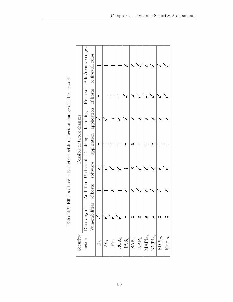
Chapter 4. Dynamic Security Assessments
Tab
le4.
7:E
ffec
tsof
secu
rity
met
rics
wit
hre
spec
tto
chan
ges
inth
enet
wor
k
Sec
uri
ty
met
rics
Pos
sible
net
wor
kch
ange
s
Dis
cove
ryof
Vuln
erab
ilit
ies
Addit
ion
ofhos
ts
Up
dat
eof
soft
war
e
Dis
abling
applica
tion
Inst
alling
applica
tion
Rem
oval
ofhos
ts
Add/r
emov
eed
ges
orfire
wal
lru
les
Rt i
!�
!�
!�
�
ACt i
!�
!�
!�
�
Pr ti
!7
!�
��
�
RO
At i
!�
!�
!�
�
PSSt i
�!
��
!!
7
SA
Pt i
77
77
77
7
NA
Pt i
7!
!�
7!
!
MA
PLt i
7!
!�
7!
!
NM
PLt i
7!
!�
7!
!
SD
PLt i
7!
!�
7!
!
MoP
Lt i
77
!�
7!
!
90
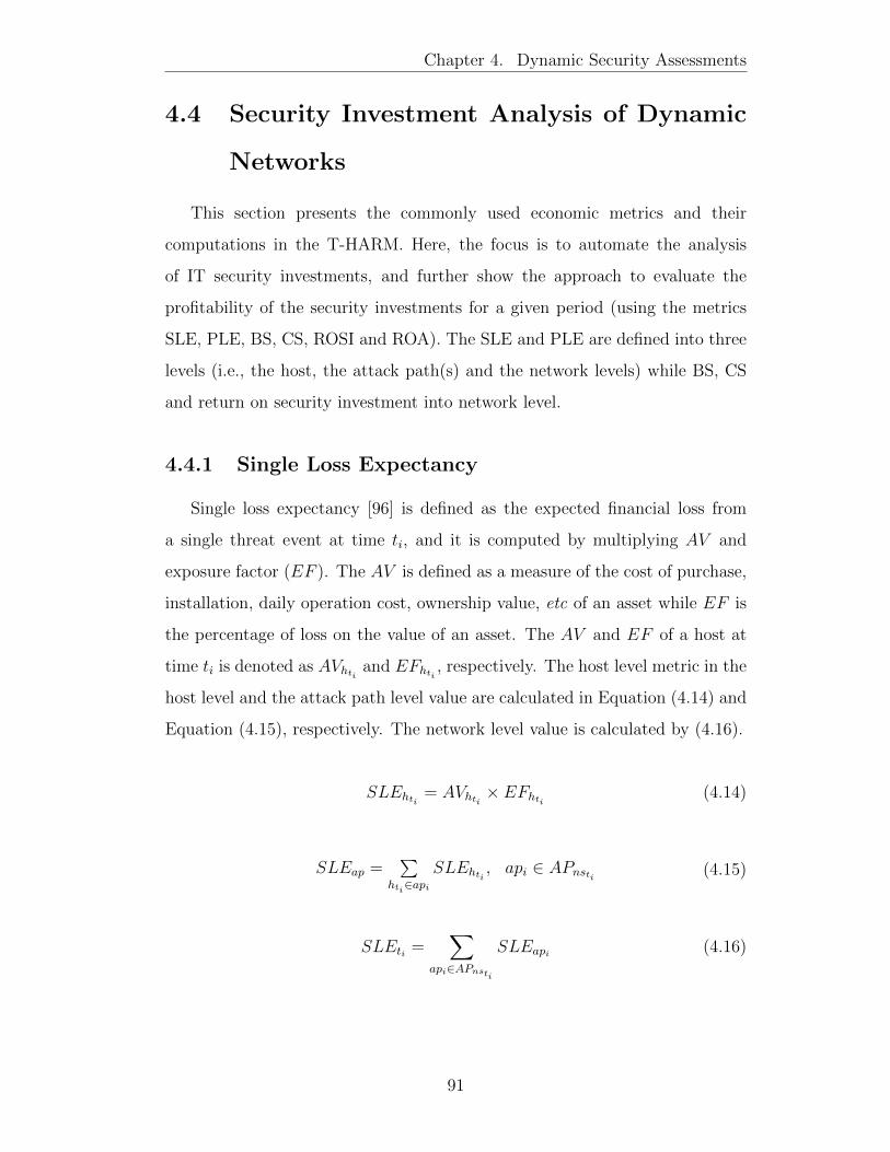
Chapter 4. Dynamic Security Assessments
4.4 Security Investment Analysis of Dynamic
Networks
This section presents the commonly used economic metrics and their
computations in the T-HARM. Here, the focus is to automate the analysis
of IT security investments, and further show the approach to evaluate the
profitability of the security investments for a given period (using the metrics
SLE, PLE, BS, CS, ROSI and ROA). The SLE and PLE are defined into three
levels (i.e., the host, the attack path(s) and the network levels) while BS, CS
and return on security investment into network level.
4.4.1 Single Loss Expectancy
Single loss expectancy [96] is defined as the expected financial loss from
a single threat event at time ti, and it is computed by multiplying AV and
exposure factor (EF ). The AV is defined as a measure of the cost of purchase,
installation, daily operation cost, ownership value, etc of an asset while EF is
the percentage of loss on the value of an asset. The AV and EF of a host at
time ti is denoted as AVhti and EFhti , respectively. The host level metric in the
host level and the attack path level value are calculated in Equation (4.14) and
Equation (4.15), respectively. The network level value is calculated by (4.16).
SLEhti = AVhti × EFhti (4.14)
SLEap =∑
hti∈apiSLEhti , api ∈ APnsti (4.15)
SLEti =∑
api∈APnsti
SLEapi (4.16)
91

Chapter 4. Dynamic Security Assessments
4.4.2 Periodic Loss Expectancy
Periodic loss expectancy is based on annual loss expectancy [96]. This is
defined as the expected financial loss due to an attack event. It is computed
by multiplying the SLE and the attack rate of occurrence for that period
(commonly known as ARO [14]. However, it is used as the PRO). The PRO
is defined as the likelihood that a risk will occur at a particular time. Here, the
PRO values for vulnerabilities in AT are calculated by equation (4.17) (using
AND and OR gates). The PROhtiand PLEap
ti values for hosts and attack paths
are computed by equation (4.18) and (4.19), respectively. Then, the network
level value is calculated by equation (4.20).
PRObti=
∏
v∈cti (bti )PROv,
bti∈Btigti (bti )=AND
1−∏
v∈cti (bti )PROv,
bti∈Btigti (bti )=OR
(4.17)
PROhti= PROrootti
(4.18)
PLEapiti =
∑hti∈api
SLEhti × PROhti, api ∈ APnsti (4.19)
PLEti =∑
api∈APnsti
PLEapiti (4.20)
4.4.3 Benefit of Security
Benefit of Security [14] is used to quantify the possible benefit of
implementing a countermeasure. It is the difference between the loss
expectancy without security and the loss expectancy with security. This metric
is denoted as BS and compute it by equation (4.21). Here, PLEbefore and
PLEafter is the security level before countermeasures and after countermeasures
92
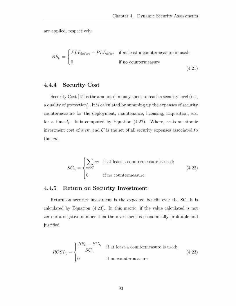
Chapter 4. Dynamic Security Assessments
are applied, respectively.
BSti =
PLEbefore − PLEafter if at least a countermeasure is used;
0 if no countermeasure
(4.21)
4.4.4 Security Cost
Security Cost [15] is the amount of money spent to reach a security level (i.e.,
a quality of protection). It is calculated by summing up the expenses of security
countermeasure for the deployment, maintenance, licensing, acquisition, etc.
for a time ti. It is computed by Equation (4.22). Where, cs is an atomic
investment cost of a cm and C is the set of all security expenses associated to
the cm.
SCti =
∑cs∈C
cs if at least a countermeasure is used;
0 if no countermeasure
(4.22)
4.4.5 Return on Security Investment
Return on security investment is the expected benefit over the SC. It is
calculated by Equation (4.23). In this metric, if the value calculated is not
zero or a negative number then the investment is economically profitable and
justified.
ROSIti =
BSti − SCti
SCtiif at least a countermeasure is used;
0 if no countermeasure
(4.23)
93

Chapter 4. Dynamic Security Assessments
4.4.6 Return on Attack
The return on attack [34] is a metric used to quantify the benefit for the
attacker when the attacker successfully exploits a vulnerabilities. This metric is
calculated using Equation (4.27). The aimv, acv, and prv value are calculated
for each vulnerability in AT using AND and OR gates by equation (4.24). The
host return on attack value (roah) is given by equation (4.25), the attack path
value is given by equation (4.26) and the network-level value ROAti is then
given by Equation (4.27).
roabti =
∑
vti∈cti (bti )
prvti×aimvtiacvti
, bti∈Btigti (bti )=AND
maxvti∈cti (bti )
prvti×aimvtiacvti
, bti∈Btigti (bti )=OR
(4.24)
roahti = roaroot (4.25)
roaapiti =∑
hti∈api
prhti×aimhtiachti
, api ∈ APnsti (4.26)
ROAti =∑
api∈APnsti
roaapiti (4.27)
Economic index: Economic values are assigned to the components (i.e.,
hosts and vulnerabilities) of the T-HARM, these values are based on the
statistical data collected in [14] (the data were collected from the CSI Computer
and Security Survey [135] and 2009 Global Security Survey [18]). So, the AV
used for information stored on a server is $11290 (per period), and $1050 for
user workstations and their EF is 0.06. Based on the CVSS exploitability
subscore and BS [35], value are assigned to PRO, pr, aim and ac for each
vulnerabilities, respectively. The summary of the vulnerabilities metrics is
shown in Table 4.8. These values are used along with the economic index to
calculate the various economic metrics described in section 4.2.1.
94
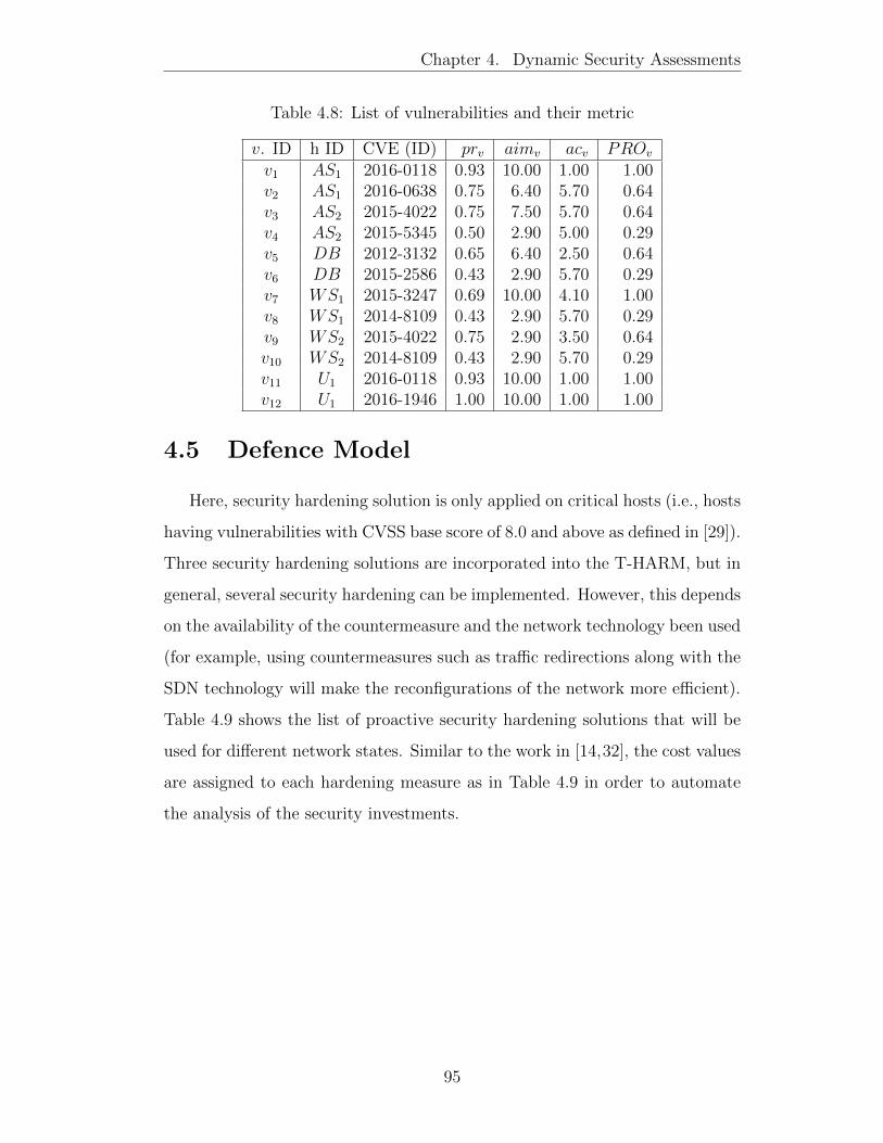
Chapter 4. Dynamic Security Assessments
Table 4.8: List of vulnerabilities and their metric
v. ID h ID CVE (ID) prv aimv acv PROv
v1 AS1 2016-0118 0.93 10.00 1.00 1.00v2 AS1 2016-0638 0.75 6.40 5.70 0.64v3 AS2 2015-4022 0.75 7.50 5.70 0.64v4 AS2 2015-5345 0.50 2.90 5.00 0.29v5 DB 2012-3132 0.65 6.40 2.50 0.64v6 DB 2015-2586 0.43 2.90 5.70 0.29v7 WS1 2015-3247 0.69 10.00 4.10 1.00v8 WS1 2014-8109 0.43 2.90 5.70 0.29v9 WS2 2015-4022 0.75 2.90 3.50 0.64v10 WS2 2014-8109 0.43 2.90 5.70 0.29v11 U1 2016-0118 0.93 10.00 1.00 1.00v12 U1 2016-1946 1.00 10.00 1.00 1.00
4.5 Defence Model
Here, security hardening solution is only applied on critical hosts (i.e., hosts
having vulnerabilities with CVSS base score of 8.0 and above as defined in [29]).
Three security hardening solutions are incorporated into the T-HARM, but in
general, several security hardening can be implemented. However, this depends
on the availability of the countermeasure and the network technology been used
(for example, using countermeasures such as traffic redirections along with the
SDN technology will make the reconfigurations of the network more efficient).
Table 4.9 shows the list of proactive security hardening solutions that will be
used for different network states. Similar to the work in [14,32], the cost values
are assigned to each hardening measure as in Table 4.9 in order to automate
the analysis of the security investments.
95

Chapter 4. Dynamic Security Assessments
Table 4.9: List of countermeasures
time cm ID cm name cs ($)
t1
cm1 Vulnerability patching 1300.00
cm2 Traffic redirection 975.00
cm3 Host isolation 650.00
t2
cm1 Vulnerability patching 1300.00
cm2 Traffic redirection 975.00
cm3 Host isolation 650.00
4.6 Simulations and Results Analysis
GSMs with economic metrics can be used to automate the analysis of IT
investment. This section automates and analyses the profitability of security
investments over a period of time via simulations. In the simulations, different
economic metrics are computed using the T-HARM. Two network states similar
to the one shown in Figure 3.1 is used. However, there are 5 hosts in the first
state, which consists of WS2, AS1, AS2, User1 and DB (i.e., the network states
at time t1), and 6 hosts in the second network states which consists of WS1,
WS2, AS1, AS2, User1 and DB (i.e., the network states at time t2). The
metrics, as well as their computations, are shown in Section 4.4. Also, the
countermeasures described in section 4.5 are used as the defence mechanisms.
Additionally, for all the scenarios the vulnerabilities that are found for the
OSes and applications in Table 3.1 are used. For the vulnerabilities, related
data are collected from the NVD [118] (the list of the vulnerabilities is found
in Table 4.8.
The T-HARM for the different network states is constructed via
simulations, using the reachability information of the example network and
the vulnerabilities. The simulations are performed in two scenarios; Scenario
I and Scenario II. The former scenario aims to demonstrate how T-HARM
is used to evaluate the profitability of IT investments given different network
states (i.e., for a period of time). The latter one shows the selection of the best
countermeasure in the different network states.
96
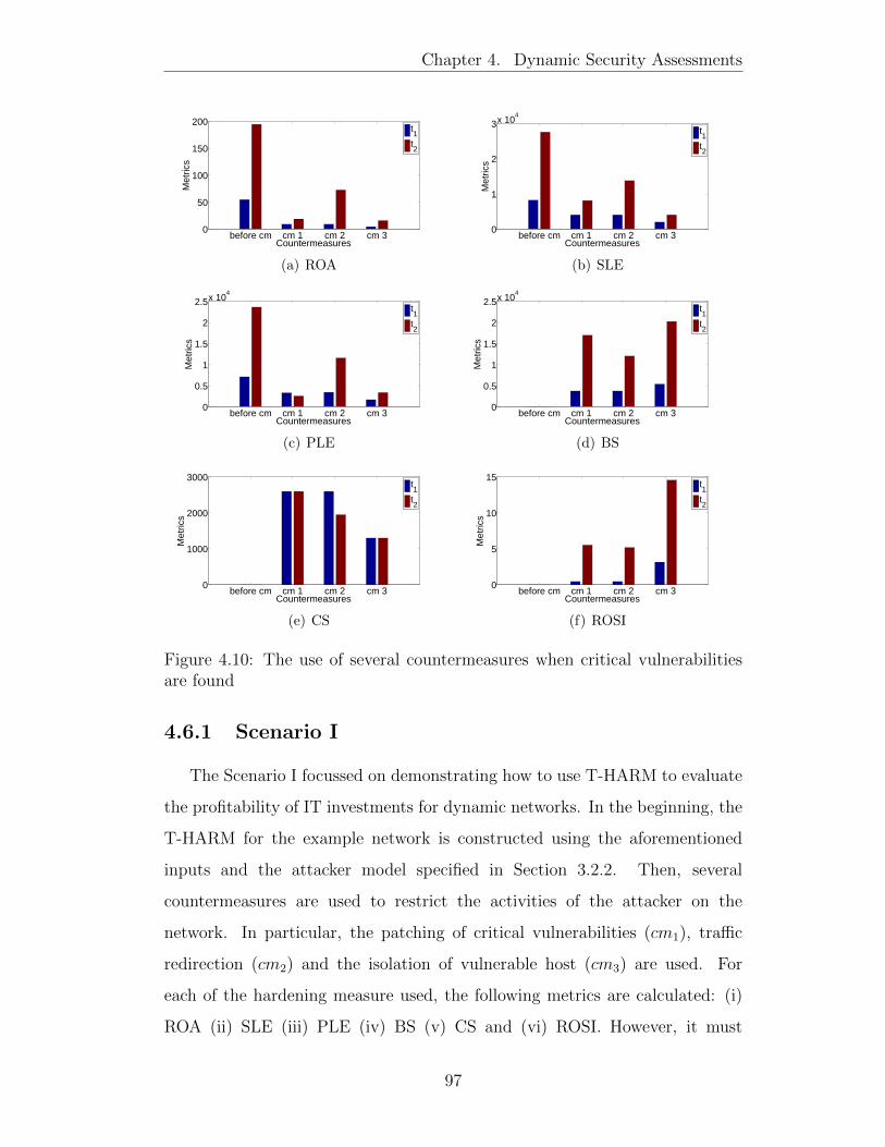
Chapter 4. Dynamic Security Assessments
before cm cm 1 cm 2 cm 30
50
100
150
200
Countermeasures
Met
rics
t1t2
(a) ROA
before cm cm 1 cm 2 cm 30
1
2
3x 10⁴
Countermeasures
Met
rics
t1t2
(b) SLE
before cm cm 1 cm 2 cm 30
0.5
1
1.5
2
2.5x 10⁴
Countermeasures
Met
rics
t1t2
(c) PLE
before cm cm 1 cm 2 cm 30
0.5
1
1.5
2
2.5x 10⁴
Countermeasures
Met
rics
t1t2
(d) BS
before cm cm 1 cm 2 cm 30
1000
2000
3000
Countermeasures
Met
rics
t1t2
(e) CS
before cm cm 1 cm 2 cm 30
5
10
15
Countermeasures
Met
rics
t1t2
(f) ROSI
Figure 4.10: The use of several countermeasures when critical vulnerabilitiesare found
4.6.1 Scenario I
The Scenario I focussed on demonstrating how to use T-HARM to evaluate
the profitability of IT investments for dynamic networks. In the beginning, the
T-HARM for the example network is constructed using the aforementioned
inputs and the attacker model specified in Section 3.2.2. Then, several
countermeasures are used to restrict the activities of the attacker on the
network. In particular, the patching of critical vulnerabilities (cm1), traffic
redirection (cm2) and the isolation of vulnerable host (cm3) are used. For
each of the hardening measure used, the following metrics are calculated: (i)
ROA (ii) SLE (iii) PLE (iv) BS (v) CS and (vi) ROSI. However, it must
97
Chapter 4. Dynamic Security Assessments
be noted that before applying any of the hardening measures, the different
metrics are calculated first (and the results are shown with ‘before cm’). Then,
one hardening measure is used per time, and the results are shown using the
hardening measures’ (countermeasures’) names per time in graphs.
Figure 4.10 shows the results for the simulations. Figure 4.10(a) shows the
results for ROA. The ROA shows the attackers’ expected gain when he is able
to compromise the target hosts. From the graph, the attacker has the most
gain if no countermeasure(s) is used for both of the network states (i.e., t1 and
t2). Similarly, the results show that the attacker will be having more gain if
he compromise the target at t2 compared to t1 (i.e., for ’before cm’, cm1, cm2
and cm3). From the defenders’ perspective, using cm1 and cm2 at t1 produce
the same results hence, either of them has the same effects in reducing the
attackers gain. Further, it is observed that using cm3 will optimally reduce the
attacker gain the most while using cm1 will allow the attacker to have more
gain compared to the other countermeasures.
Figure 4.10(b) presents the results for the SLE. The results show the
expected financial loss in consequence of a single attack event. From the
results, it is observed that both states have varying SLE value. However,
the SLE value for the before countermeasures is higher. Conversely, when the
various hardening measures are used, the result shows that the SLE values
decrease for both t1 and t2 states (with cm3 being the best for both states).
In Figure 4.10(c), the results show the expected financial loss taking into
account multiple states (i.e., the period a countermeasure is used compared
to its previous network state). For this metric, similar results are observed for
the SLE. However, for the PLE the use of cm3 and cm1 can reduce the PLE
the most at t1 and t2, respectively.
Subsequently, the results for ‘before cm’ is zero in Figure 4.10(d), 4.10(e)
and 4.10(f). This is for the reason that, there is no countermeasure use at
that points. However, for the other points when countermeasure is used, the
BS, CS, and the ROSI are improved compared to former. In addition, at t1,
98
Chapter 4. Dynamic Security Assessments
cm1 and cm2 have the same BS for the defender while cm3 is the having the
maximum benefit for the defender. At t2, all the countermeasures have varying
values with cm3 returning the maximum benefit for the defender also, then
followed by cm1 and cm2, respectively.
In Figure 4.10(e), cm1 and cm3 have the same CS for t1 while at t2, they
both have varying values. However, the cm3 is having the same CS for both
states (and it is the minimal CS for the defender). Similarly, in Figure 4.10(f),
using either cm1 or cm2 can give the defender a similar ROSI value for both
states. In summary, it is observed observe that different network states can
have varying optimal countermeasures based on the different metrics.
4.6.2 Scenario II
Scenario II automates the analysis of the optimal countermeasures at
different time points given a metric. In Algorithm 2, the selection of the
optimal countermeasure (for T-HARM) from a set of countermeasures per time
is described. Here, only ROSI is used (this is to capture the cost and benefits
for the defender perspective). The Algorithm 2 is used for this simulations.
The algorithm presents how to select the optimal countermeasure from a set of
countermeasures. The input in the algorithm is a set of network states NS, a
set of countermeasures, and a set of vulnerabilities. First, the algorithm starts
by applying each countermeasure to the set of critical vulnerability found on
every host. Then, the ROSI is calculated for each of the countermeasures used.
Subsequently, the optimal countermeasure is selected based on the ROSI. This
process is done for all network state nsti belonging to the set of states NS, and
finally, the set of optimal solutions is returned.
The results for this simulation are shown in Table 4.10. And based on the
algorithm, the optimal solution is cm3 with ROSI of 3.16 and 14.58 at t1 and t2,
respectively. Therefore, a conclusion can be made that, it is financially justified
to use cm3 compared to cm1 and cm2 for the network.
99
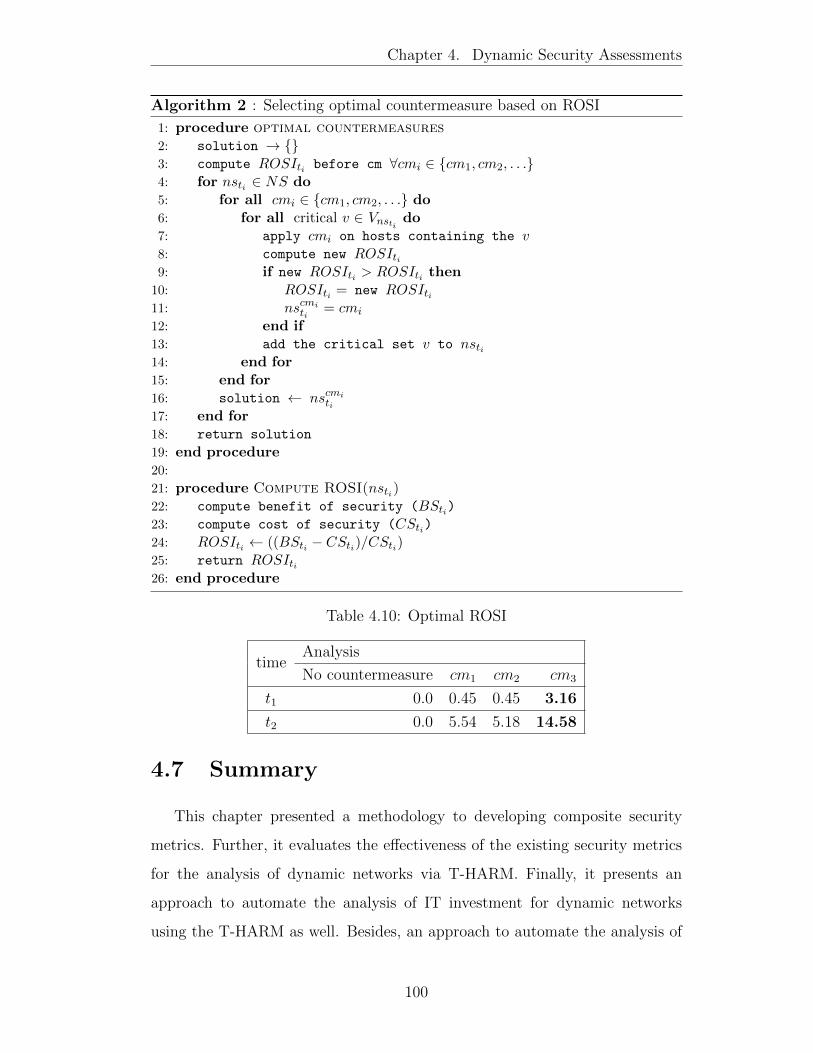
Chapter 4. Dynamic Security Assessments
Algorithm 2 : Selecting optimal countermeasure based on ROSI
1: procedure optimal countermeasures2: solution → {}3: compute ROSIti before cm ∀cmi ∈ {cm1, cm2, . . .}4: for nsti ∈ NS do5: for all cmi ∈ {cm1, cm2, . . .} do6: for all critical v ∈ Vnsti do7: apply cmi on hosts containing the v8: compute new ROSIti9: if new ROSIti > ROSIti then
10: ROSIti = new ROSIti11: nscmiti
= cmi
12: end if13: add the critical set v to nsti14: end for15: end for16: solution ← nscmiti17: end for18: return solution
19: end procedure20:
21: procedure Compute ROSI(nsti)22: compute benefit of security (BSti)23: compute cost of security (CSti)24: ROSIti ← ((BSti − CSti)/CSti)25: return ROSIti26: end procedure
Table 4.10: Optimal ROSI
timeAnalysis
No countermeasure cm1 cm2 cm3
t1 0.0 0.45 0.45 3.16
t2 0.0 5.54 5.18 14.58
4.7 Summary
This chapter presented a methodology to developing composite security
metrics. Further, it evaluates the effectiveness of the existing security metrics
for the analysis of dynamic networks via T-HARM. Finally, it presents an
approach to automate the analysis of IT investment for dynamic networks
using the T-HARM as well. Besides, an approach to automate the analysis of
100

Chapter 4. Dynamic Security Assessments
IT security investments, and the approach to exhaustively compute the optimal
security investment (from a given set of hardening measure based on a metric
ROSI) for every network states is demonstrated.
101
Chapter 5
Time-Independent HARM
There are three main approaches to capture changes using the GSM for the
dynamic networks, which are time-driven, event-driven or user-driven. In the
case of the time-driven approach, the GSM is constructed at predefined times.
In case of the event-driven approach, the GSM is constructed when changes
have been detected. In the case of the user-driven approach, a user decides
which times the GSM is constructed. These approaches can be used to generate
multiple GSM snapshots (e.g., the temporal GSMs), with each snapshot with
different security properties for that particular network state within a given
time window [19]. However, the existing modelling approaches lack methods
and techniques to represent the overall security posture of dynamic networks
using a representative GSM or metric value.
In order to have an overall overview of the security of dynamic networks, one
must take into account all observable attributes of dynamic networks, which
includes multiple network states, the duration of each state and the visibility
of components over time.
In this chapter, TI-HARM is proposed to present the overall overview of the
security of dynamic networks. The idea is to capture dynamic network states
at various times, and then aggregate them taking into account the attributes
of the dynamic network. The difference between the temporal GSM and the
time-independent GSM is, the temporal GSM models the security states of
102
Chapter 5. Time-Independent HARM
the dynamic networks onto multiple GSM at every time t while the time-
independent GSM (i.e., TI-HARM) models the security of dynamic networks
onto a single GSM (regardless of time and states). The TI-HARM not only
assess the security of each network state, but also identify and assess all
potential attack paths in the multiple network states, as well as attack events
happening over multiple network states (to one GSM). The approach used in
this chapter aggregates network states for security modelling and analysis for
the dynamic network taking into account various dynamic attributes. The
main contributions of this chapter are as follows:
� Develop a time-independent GSM by incorporating multiple network
states and their dynamic attributes;
� Formally define TI-HARM;
� Propose a security rating system based on weight optimisation algorithm
using the TI-HARM;
� Demonstrate the feasibility of the approach in experimental analysis via
simulations.
5.1 Network and Attacker Model
To demonstrate this approach, a three-tier enterprise network (i.e.,
consisting of DMZ, subnets, firewall, web server which is accessible from the
public Internet, etc) and attacker model which is similar to the one in Figure 3.1
and in Figure 3.2.2 is used, respectively. The initial network consists of eight
hosts located in three subnets; DMZ, internal network and the Database (DB)
subnet. The subnets are divided by firewalls which control access from one
subnet to another. However, the machines in the DMZ passively receive all
service requests from the Internet then respond appropriately. Here, it is
assumed that the machine names do not change for the period considered. In
103

Chapter 5. Time-Independent HARM
Figure 5.1, the topologies for the network captured when changes are observed
in the network (i.e., event-driven approach) are shown. The descriptions of the
topologies are given as follows; (a) ns0 topology: The initial network topology
with a state duration = 2 mins. (b) ns1 topology: The connection between
WS1 and U3 is removed, and the state duration = 4 mins. (c) ns2 topology:
Host U3 is removed from the network as well as its edges, and the state duration
= 4 mins. (d) ns3 topology: Host U4 is added to the network, and the state
duration = 5 mins. (e) ns4 topology: Edge between WS1 and U2 is added to
the network, and state duration = 4 mins. (f) ns5 topology: Hosts WS2 is
removed from the network, and state duration = 5 mins. The different states
have the vulnerabilities listed in Table 5.1.
Table 5.1: List of vulnerabilities for the example network along with theirmetrics
v ID prv aimv
v1 0.43 5.50
v2 1.00 10.00
v3 0.75 7.00
v4 0.43 5.50
v5 0.72 10.00
v6 0.43 4.00
v7 0.90 9.00
v8 0.50 5.00
v9 0.20 2.00
v10 0.88 8.00
v11 0.43 6.00
104
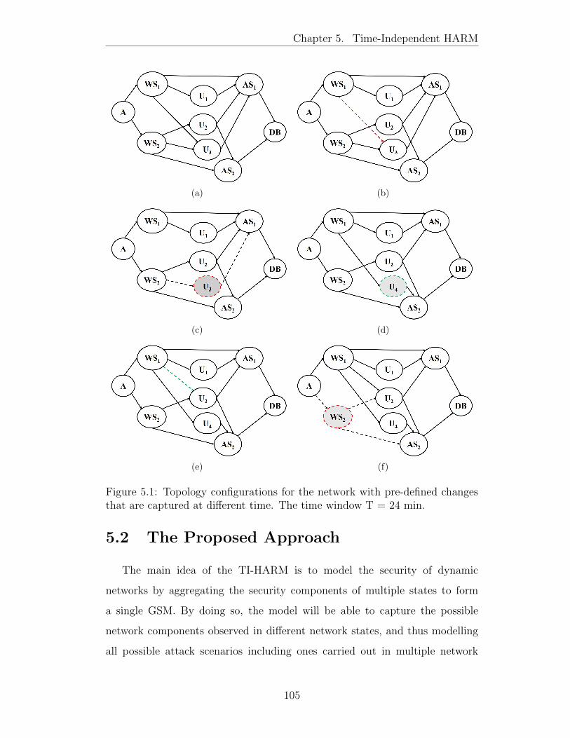
Chapter 5. Time-Independent HARM
(a) (b)
(c) (d)
(e) (f)
Figure 5.1: Topology configurations for the network with pre-defined changesthat are captured at different time. The time window T = 24 min.
5.2 The Proposed Approach
The main idea of the TI-HARM is to model the security of dynamic
networks by aggregating the security components of multiple states to form
a single GSM. By doing so, the model will be able to capture the possible
network components observed in different network states, and thus modelling
all possible attack scenarios including ones carried out in multiple network
105

Chapter 5. Time-Independent HARM
states.
In this section, the description and the construction of the TI-HARM for the
analysis of dynamic networks are provided. The following network properties
are taken into account; multiple network states, time duration of states
and the visibility of network components in the states to construct the TI-
HARM. Specifically, the changes associated with hosts and their reachability
information in multiple states are considered. This is because the structure of
the network system (i.e., the hosts reachability) is important for some type of
progressive attacks (e.g., sequential attacks) [72].
In the TI-HARM, the components have weight values based on their
visibility over time (where a component that appears more frequently will
have a higher weight value). This approach can allow network administrators
to perform other security analysis on network components with different
visibilities. For example, more static network components are exposed to the
attackers, allowing them to discover vulnerabilities and plan an attack that
would still be viable in time. For this fact, the network administrator can use
the TI-HARM to discover such static components in order to mitigate such
attacks.
The calculations for the weight value is formulated in equation (5.1). The TI-
HARM is described in Section 5.2.1. Then, in Section 5.2.2, the construction
of the TI-HARM with different weight values is shown for the network states
in Figure 5.1.
ncαj =
(OCncj|NS|
×∑|NS|
i=0 t(ncj)
T
)× 100 (5.1)
5.2.1 Formalism of TI-HARM
In this section, the descriptions and formalism of TI-HARM is presented.
The TI-HARM is described in terms of H, E and V as follows:
� Each host hi∈H has a weight value hαi that is calculated based on the
106

Chapter 5. Time-Independent HARM
visibility of the host in the network states (such that 0 ≤ hαi ≤ 100), a
set of weighted adjacent hosts hadji ⊆H, a host type htypei ∈ {web server,
app server, user workstation}, a set of vulnerabilities hvi⊆V , and a set of
security metrics hmetricsi ∈{attack cost, attack risk, ROSI, . . .}.
� Each edge ei ∈ E has a weight value eαi that is calculated based on its
visibility in the network states as well (with 0 ≤ eαi ≤ 100).
� Each vulnerability v∈V has a privilege level that is acquired by the
attacker after the vulnerability is successfully exploited vprivilege∈{root,
user, ...} and a set of security metrics vmetrics∈{attack cost, attack risk,
. . .}.
The TI-HARM is described as two layered GSM; the upper layer and
the lower layer. The upper layer captures the temporal hosts’ reachability
information and the attacker’s entry points (using AG) while the lower layer
captures the vulnerability information of each hosts using ATs. The TI-HARM
is formally defined as follows.
Definition 11. The TI-HARM is a 4-tuple TI − HARM = (U,L,C,w)
which is constructed based on the calculated weight values of network states
components that are equal or below the weight value threshold w (the calculation
of the weight value is shown in Equation(5.1)). Here, U is the upper layer (AG)
that models the set of hosts H and their reachability information, and L is the
lower layer (ATs) that models the set of vulnerabilities V for each host hi ∈ H,
respectively. The mapping between the upper and the lower layers is defined as
C ⊆ {(hi ↔ AT )}∀hi ∈ U,AT ∈ L.
Next, the upper layer and the lower layer are defined in Definition (12) and
Definition (13), respectively.
Definition 12. The upper layer of the TI-HARM is a 3-tuple (H,E,w), where
H is a finite set of weighted hosts in the upper layer where hi ∈ H and hαi ≤ w,
107

Chapter 5. Time-Independent HARM
E ⊆ H ×H is a set of weighted edges where ei ∈ E and eαi ≤ w, and w is the
calculated weight threshold value.
Definition 13. The lower layer of the TI-HARM is a set of ATs. Here, AT
is a 5-tuple AT=(A, B, c, g, root), where A ⊆ V is a set of vulnerabilities,
B = {b1, b2, . . .} is a set of gates, c ⊆ {bj → el}∀bj ∈ B, el ∈ A∪B is a mapping
of gates to vulnerabilities and other gates, g ⊆ {bj→{AND,OR}} specifies the
type of each gate, and root∈A∪B is the root node of the AT .
5.2.2 Constructing TI-HARM
To fully understand the security of a dynamic network, it is important to
take into account changes in the networks (for an effective security analysis).
Therefore, an approach that takes into account changes associated with hosts,
their connections and their duration is developed. The approach (i.e., the
construction of the TI-HARM) is described using Algorithm 3, Algorithm 4 and
Algorithm 5. In particular, Algorithm 3 and Algorithm 4 show the calculations
of weight values for the hosts and edges, respectively. Algorithm 5 show the
construction of the TI-HARM. An example network is used to describe the
construction of the TI-HARM. In specific, the network topologies in Figure 7.1
are used, and the equation 5.1 is used to calculate the weight value for each
components.
Algorithm 3 Algorithm for computing hosts’ weight value
1: procedure Weight Hosts(NS)2: H → {}3: for all nsi ∈ NS do4: H = H ∪ {hi, ∀hi ∈ nsi}5: end for6: for each hi ∈ H do7: ncαhi = (OCnchi/|NS|)× (
∑|NS|i=0 t(nchi)/T )× 100
8: hαi ← ncαhi9: end for
10: end procedure
108

Chapter 5. Time-Independent HARM
Table 5.2: The calculated weight values for hosts
Host name (ncj) AS1 AS2 WS1 WS2 U1 U2 U3 U4 DB
OCncj 6 6 6 5 6 6 2 3 6∑|NS|i=0 t(ncj) 24 24 24 19 24 24 6 14 24
OCncj|NS| 1.00 1.00 1.00 0.83 1.00 1.00 0.33 0.50 1.00∑|NS|i=0 t(ncj)
T 1.00 1.00 1.00 0.79 1.00 1.00 0.25 0.58 1.00(OCncj|NS| ×
∑|NS|i=0 t(ncj)
T
)× 100 100 100 100 66 100 100 8.33 29 100
Algorithm 4 Algorithm for computing edges’ weight value
1: procedure Weight Edges(NS)2: E → {}3: for all nsi ∈ NS do4: for each hi ∈ si do5: eN= Get set of edges for a node(hi)6: for each ei ∈ eN do7: if ei not in E then8: add ei to E9: end if
10: end for11: end for12: end for13: for each ei ∈ E do14: ncαei = (OCncei/|NS|)× (
∑|NS|i=0 t(ncei)/T )× 100
15: eαi ← ncαei16: end for17: end procedure
Table 5.2 and Table 5.3 show the detailed calculations for the hosts and
edges from the network topologies, respectively. The weight value shows how
each component appears in the network states for the time window (i.e., T=24
mins). In Figure (5.2), the construction of the TI-HARM (using different weight
values) for states (in Figure 7.1) is demonstrated. Specifically, Figure 5.2(a)
show the TI-HARM with w = 0.0%. This shows the extreme cases where the
TI-HARM captures all the observed components from all network states. In
this case, it can be said that all the possible attack scenarios are well captured.
Figure 5.2(b) captures only network component that are visible for half of the
entire time window (i.e., w = 50.0%). Figure 5.2(c) captures the network
109
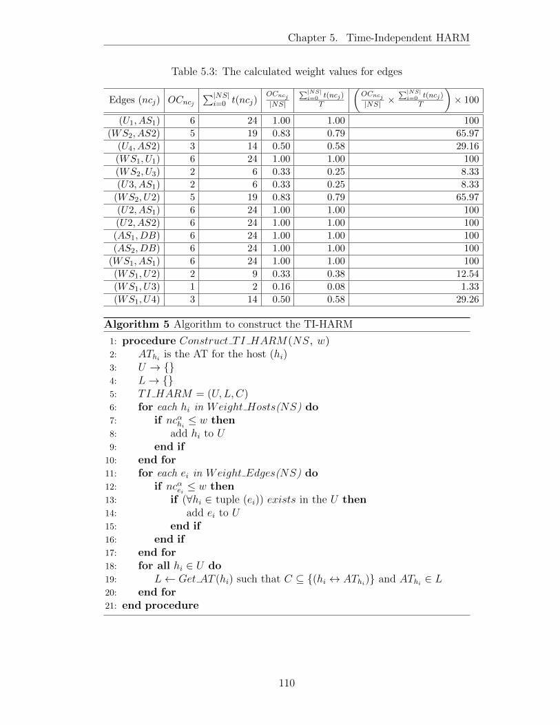
Chapter 5. Time-Independent HARM
Table 5.3: The calculated weight values for edges
Edges (ncj) OCncj∑|NS|
i=0 t(ncj)OCncj|NS|
∑|NS|i=0 t(ncj)
T
(OCncj|NS| ×
∑|NS|i=0 t(ncj)
T
)× 100
(U1, AS1) 6 24 1.00 1.00 100
(WS2, AS2) 5 19 0.83 0.79 65.97
(U4, AS2) 3 14 0.50 0.58 29.16
(WS1, U1) 6 24 1.00 1.00 100
(WS2, U3) 2 6 0.33 0.25 8.33
(U3, AS1) 2 6 0.33 0.25 8.33
(WS2, U2) 5 19 0.83 0.79 65.97
(U2, AS1) 6 24 1.00 1.00 100
(U2, AS2) 6 24 1.00 1.00 100
(AS1, DB) 6 24 1.00 1.00 100
(AS2, DB) 6 24 1.00 1.00 100
(WS1, AS1) 6 24 1.00 1.00 100
(WS1, U2) 2 9 0.33 0.38 12.54
(WS1, U3) 1 2 0.16 0.08 1.33
(WS1, U4) 3 14 0.50 0.58 29.26
Algorithm 5 Algorithm to construct the TI-HARM
1: procedure Construct TI HARM(NS, w)2: AThi is the AT for the host (hi)3: U → {}4: L→ {}5: TI HARM = (U,L,C)6: for each hi in Weight Hosts(NS) do7: if ncαhi ≤ w then8: add hi to U9: end if
10: end for11: for each ei in Weight Edges(NS) do12: if ncαei ≤ w then13: if (∀hi ∈ tuple (ei)) exists in the U then14: add ei to U15: end if16: end if17: end for18: for all hi ∈ U do19: L← Get AT (hi) such that C ⊆ {(hi ↔ AThi)} and AThi ∈ L20: end for21: end procedure
110
Chapter 5. Time-Independent HARM
components that are visible for all the times in the states (i.e., the components
that have a weight value of 100%. This is also the other extreme where only
the most persistent components for the entire time window are captured).
5.2.3 Security Metrics Calculations
In the TI-HARM, several security metrics can be implemented to analyse
the security of dynamic networks. However, in this section, only the following
are used; (i) Risk on attack paths (ii) Probability of attack success on paths
and (iii) Number of attack paths. The calculation details for those metrics can
be found in Chapter 4.
5.2.4 Determining the Minimum Weight Threshold to
use for TI-HARM
Depending on the configurations and operational requirements of networks,
attack scenarios vary vastly. For example, a dynamic network with minimal
change over time would present similar weaknesses and vulnerabilities more
persistently in comparison to a dynamic network with many components
changing more frequently. Therefore, there is no single value of the weight
value to be used with the TI-HARM that can be used globally, rather more
adaptive means of choosing the weight value is needed. This is important as
choosing a wrong weight value may result in misleading security analysis if the
core network components forming the attack scenarios are not captured and
modelled. To address this problem, a MWT algorithm shown in Algorithm 6 is
developed. The algorithm computes the weight value that guarantees at least
one attack path is present. By doing so, it can carry out security analysis taking
into account the most persistent network components (i.e., network components
that appears the most across the network states). In the algorithm, r threshold
and step intv is used to represent the required threshold and for the interval
in which the weight value is adjusted, respectively.
111

Chapter 5. Time-Independent HARM
(a)
(b)
(c)
Figure 5.2: TI-HARM (a) TI-HARM with w = 0.0% (i.e., all the appearance ofcomponents), (b) TI-HARM with w = 50%, and (c) TI-HARM with w = 100%
112

Chapter 5. Time-Independent HARM
Algorithm 6 Minimum weight threshold computation
1: procedure Cal min value(S, step intv, r threshold)2: set w = 0.03: minimum w→ w4: while w ≤ 100 do5: TI HARM = TI HARM(S,w)6: if attack paths exist in TI HARM then7: increment w by the step intv8: else9: minimum w ← w − step intv
10: break11: end if12: break13: end while14: TI HARM = TI HARM(S, 0.0)15: New TI HARM = New TI HARM(S, minimum w)16: risk = CALCULATE RISK(TI-HARM)17: new risk = CALCULATE RISK(New TI HARM)18: threshold ← (risk - new risk)/risk19: while threshold < r threshold do20: reduce minimum w by the step intv21: threshold ← calculate new threshold for minimum w22: end while23: return minimum w24: end procedure25:
26: procedure Calculate Risk(GSM)27: Compute all possible attack paths of GSM (paths)28: max risk → 029: for all path in paths do30: new risk ← sum of risk in path31: if new risk > max risk then32: max risk=new risk33: end if34: end for35: return max risk36: end procedure
5.2.5 Security Rating System
Using the MWT algorithm shown in Algorithm 6, a security rating system
is defined for the dynamic networks. The advantage of dynamic networks
compared to the traditional static networks is the ability to implement
113
Chapter 5. Time-Independent HARM
advanced security mechanisms such as MTD to continuously change the attack
surface. Therefore, if an attack path is identified and that attack path is
visible for a long duration (i.e., appears in many network states), then such
network yields a similar security concern as of a static network. Assuming that
all vulnerabilities are equally damaging to the network, it is more secure to
change the network components more frequently. The MWT algorithm can
be used to determine the dynamicity of networks (i.e., how much changes are
observed through different network states). Equation (5.2) shows the SRS score
calculation. In the calculation, Risk is used to denote the calculated risk for w
= 0.0%, (i.e., for all appearance) and New Risk to denote the risk calculated
using the MWT value in the TI-HARM. The metric Risk on attack paths (here
used as Risk) is calculated by Equation (4.8).
SRS = (Risk − New Risk)/Risk (5.2)
Figure 5.3 shows the meaning of the threshold value calculated. The SRS
aims to provide the overview of security for network systems. From the figure,
the SRS value shows the overview of the security for a weight value use (i.e., how
the number of the vulnerable component are captured by the security model
based on risk). When the threshold is 0.0, it means that all the persistent
network component have been well captured by the weight value (this will
give a better analysis). Conversely, when the threshold value begins to move
towards 1.0, it shows that the level of the coverage is decreasing (with 1.0 as
the most critical threshold to allow). In this case, using a weight value with a
threshold value towards 1.0 will lead to a misleading security analysis (because
only a few important hosts are being considered for analysis). In Section 5.3.4,
the simulation networks is used to demonstrate the algorithm as well as the
interpretation for the threshold values in Figure 5.3. Also, the calculation of
the SRS is demonstrated as follows.
114

Chapter 5. Time-Independent HARM
Figure 5.3: Interpreting the SRS value
Risk on attack paths: This is calculated by Equation (4.8). The
calculations are shown in Table 5.4 and Table 5.5 for w = 0.0%, and w = 100%,
respectively. From the calculations, the Risk for for w = 0.0%, and w = 100%
is 39.78 and 38.27, respectively.
Table 5.4: Risk on attack paths for w = 0.0%
ID Paths Risk
ap1 A, WS1, AS1, DB 31.03
ap2 A, WS1, U1, AS1, DB 35.32
ap3 A, WS1, U2, AS2, DB 38.27
ap4 A, WS1, U3, AS1, DB 37.15
ap5 A, WS1, U4, AS2, DB 38.27
ap6 A, WS2, U2, AS2, DB 39.78
ap7 A, WS2, U3, AS1, DB 38.67
ap8 A, WS2, AS2, DB 32.54
Table 5.4 and Table 5.5 shows the calculations of the RISK, while the SRS
is calculated by Equation (5.2) as:
SRS = (39.78− 38.27)/39.78
= 0.04
Based on Figure 5.3, it can be concluded that the TI-HARM with w = 100%
has captured the core network components that were visible for a long duration
115

Chapter 5. Time-Independent HARM
in states since the SRS value is very close to the safe zone.
Table 5.5: Risk on attack paths for w = 100.0%
ID Paths Risk
ap1 A, WS1, AS1, DB 31.03
ap2 A, WS1, U1, AS1, DB 35.32
ap3 A, WS1, U2, AS2, DB 38.27
5.3 Simulations and Results
Experimental analysis via simulations is performed to demonstrate the
proposed model. Also, the appropriate weight value (for hosts and edges) to
use (for different network models) given multiple states, network components
and their duration are investigated. To generalise, two dynamic network models
(similar to Bopche and Mehtre [19]) are simulated; (i) External - DMZ - Internal
network (E - D - I network) and (ii) External - Internal network (E - I network),
these may include a subset of other complex network topology within each
subnet. The descriptions for the networks are giving in Section 5.3.1. In
Section 5.3.2, the simulations settings are described, and in Section 5.3.3 the
results are presented.
5.3.1 Scenario Description and Simulation Networks
In this section, a campus network is assumed and simulated, in which the
network is open to a large number of users and so contains several workstations.
It is assumed that the network allows workstations to join the network without
security scanning and that, dynamic host configuration protocol is used to
automatically assign IP address settings to the hosts that are joining (for
instance, BYOD). Further, the network users are allowed to install software
on their workstations, and this software may have one or more vulnerability.
Hence, this may provide platforms for the attackers to hack into the network
116

Chapter 5. Time-Independent HARM
(a)
(b)
Figure 5.4: The initial network use in simulations: (a) E - D - I network, and(b) E - I network.
then have control over sensitive resources.The description of the two network
models used is described as follows.
E-D-I network: The network is shown in Figure 5.4(a). The network
is divided into a DMZ and internal network with the attacker located on
the external network. The internal network consists of three campuses and
the database subnet. The subnets are separated by firewalls which control
access to resources found on each of the subnets. The DMZ subnet only allows
external users to have access to the web server before having access to the
Database. Further, the hosts in the internal network are allowed to send
packets to other hosts within the internal network. The outside attacker is
an authorised user who does not have permission to access sensitive data on
the database. Here, the attack goal is for the attacker to escalate privileges
from users’ to administrator’ privilege then steal sensitive data. It is assumed
that the attacker cannot reach the Database directly. However, once an attacker
117
Chapter 5. Time-Independent HARM
connects to the network through the web servers, the attacker can easily obtain
information about the network topology and vulnerabilities using tools such as
Nmap and OpenVAS.
E-I network: The network is shown Figure 5.4(b). The network consists of
only a firewall which controls access to the internal network. However, hosts in
the internal network are able to send packets to other hosts within the internal
network. It is assumed that the attacker is located on the external network and
therefore the attacker is able to reach only a few hosts (i.e., the web servers)
however, the attacker can reach other hosts once he reaches the web server.
Similarly, the attack goal here is to escalate privilege to administrators’ then
compromise the database.
5.3.2 Simulation Settings for the Network Models
The networks in Section 5.3.1 is used as the initial network state to conduct
several simulations. The initial number of hosts used for the simulation is
100. It is assumed that each host has an OS with a vulnerability as shown
in Table 5.6 (this are randomly assigned to the hosts). The following network
changes are introduced to the states, which are; (a) additions of host, (b)
removal of existing host, (c) additions of connection, and (d) removal of existing
connection, with each state has a combination of the network changes (e.g., a
state can have the combination of the changes {a,b,c,d} or {a, a, a, a}, etc).
Thus, each state has a varying number of hosts and edges. In addition, each
state has a time duration (i.e., the duration before the next network state is
captured). In this simulation, a random time duration is assigned to the states
ranging from 1 to 5 minutes. Also, ten (10) network states for every time
window (T) is simulated and used.
118
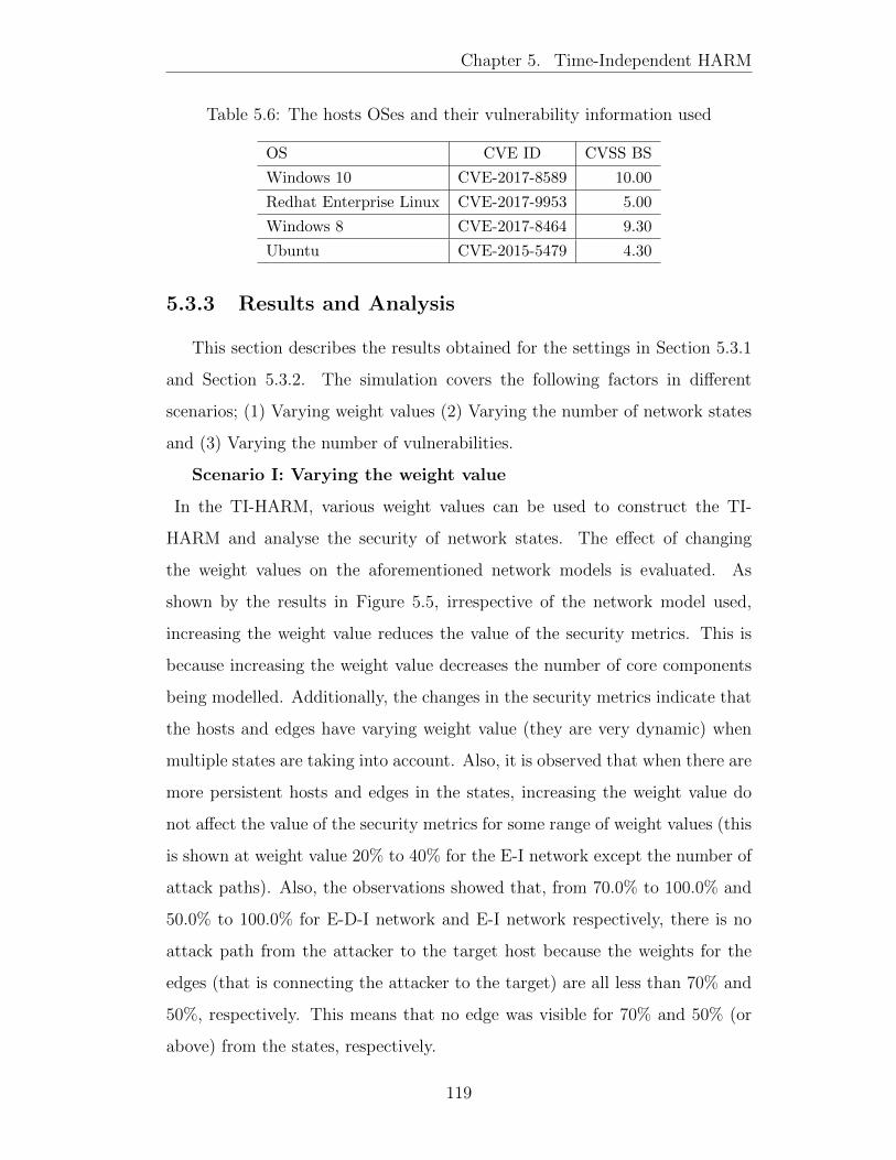
Chapter 5. Time-Independent HARM
Table 5.6: The hosts OSes and their vulnerability information used
OS CVE ID CVSS BS
Windows 10 CVE-2017-8589 10.00
Redhat Enterprise Linux CVE-2017-9953 5.00
Windows 8 CVE-2017-8464 9.30
Ubuntu CVE-2015-5479 4.30
5.3.3 Results and Analysis
This section describes the results obtained for the settings in Section 5.3.1
and Section 5.3.2. The simulation covers the following factors in different
scenarios; (1) Varying weight values (2) Varying the number of network states
and (3) Varying the number of vulnerabilities.
Scenario I: Varying the weight value
In the TI-HARM, various weight values can be used to construct the TI-
HARM and analyse the security of network states. The effect of changing
the weight values on the aforementioned network models is evaluated. As
shown by the results in Figure 5.5, irrespective of the network model used,
increasing the weight value reduces the value of the security metrics. This is
because increasing the weight value decreases the number of core components
being modelled. Additionally, the changes in the security metrics indicate that
the hosts and edges have varying weight value (they are very dynamic) when
multiple states are taking into account. Also, it is observed that when there are
more persistent hosts and edges in the states, increasing the weight value do
not affect the value of the security metrics for some range of weight values (this
is shown at weight value 20% to 40% for the E-I network except the number of
attack paths). Also, the observations showed that, from 70.0% to 100.0% and
50.0% to 100.0% for E-D-I network and E-I network respectively, there is no
attack path from the attacker to the target host because the weights for the
edges (that is connecting the attacker to the target) are all less than 70% and
50%, respectively. This means that no edge was visible for 70% and 50% (or
above) from the states, respectively.
119
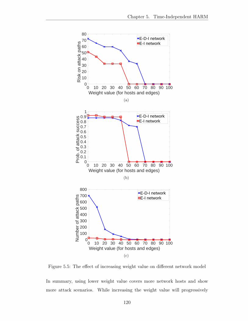
Chapter 5. Time-Independent HARM
0 10 20 30 40 50 60 70 80 90 100Weight value (for hosts and edges)
0
10
20
30
40
50
60
70
80
Ris
k on
atta
ck p
aths
E-D-I networkE-I network
(a)
0 10 20 30 40 50 60 70 80 90 100Weight value (for hosts and edges)
00.10.20.30.40.50.60.70.80.9
1
Pro
b. o
f atta
ck s
ucce
ss
E-D-I networkE-I network
(b)
0 10 20 30 40 50 60 70 80 90 100Weight value (for hosts and edges)
0
100
200
300
400
500
600
700
800
Num
ber
of a
ttack
pat
hs
E-D-I networkE-I network
(c)
Figure 5.5: The effect of increasing weight value on different network model
In summary, using lower weight value covers more network hosts and show
more attack scenarios. While increasing the weight value will progressively
120

Chapter 5. Time-Independent HARM
reduce the number of hosts and edges and will model only the more persistent
components.
Scenario II: Varying the number of states
The TI-HARM can model multiple network states with various security
property. For this simulation, the number of network states captured is varied
(ranging from two to ten states, with each state having various changes). The
network and settings in Section 5.3.1 and Section 5.3.2 is used. The weight
value w = 40.0% is carefully used for all the network states in order to ensure
that the paths from the attacker to the target hosts is not completely lost for
both network models. Here, an investigation is performed on how the number
of states captured may affect the value of metrics for the given weight value.
Figure 5.6 shows the results, given weight (w = 40.0%).
The results show that increasing the number of network states will
continuously change the representation of security posture even when the
weight value is kept constant for all cases (this is evident by the changes shown
by the security metric values in Figure 5.6). Also, it is observed that as the
number of states considered increases, the weight for the network components
reduces (this is shown by the security metric values when the following number
of states is used; 2 to 8 states and state 2 to 6 states for E-I network and E-I-D
network, respectively). Further, it is observed that in Figure 5.6(c) there is
a dramatic change in the number of attack scenarios from using 2 states to 3
states. This could be because most of the components are only visible in 1 of
the 3 states or they are having a short time duration in the states (thus, their
weight values are less than 40%). In this case, using a small number of states
may not fully show the changes in the TI-HARM.
Scenario III: Varying the number of vulnerabilities
In this section, the number of hosts vulnerabilities are varied for the simulation
networks in section 5.3.1. The aim is to investigate how the number of
vulnerabilities affects the security analysis when a given weight value is
121
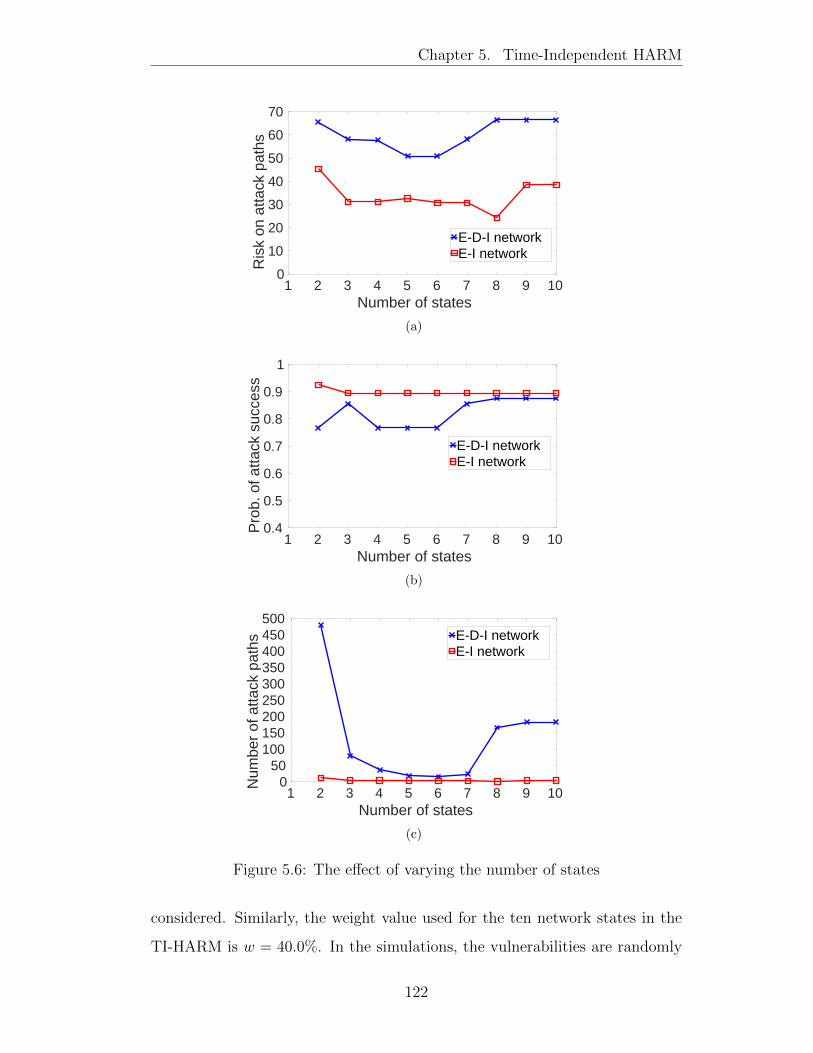
Chapter 5. Time-Independent HARM
1 2 3 4 5 6 7 8 9 10Number of states
0
10
20
30
40
50
60
70
Ris
k on
atta
ck p
aths
E-D-I networkE-I network
(a)
1 2 3 4 5 6 7 8 9 10Number of states
0.4
0.5
0.6
0.7
0.8
0.9
1
Pro
b. o
f atta
ck s
ucce
ss
E-D-I networkE-I network
(b)
1 2 3 4 5 6 7 8 9 10Number of states
050
100150200250300350400450500
Num
ber
of a
ttack
pat
hs
E-D-I networkE-I network
(c)
Figure 5.6: The effect of varying the number of states
considered. Similarly, the weight value used for the ten network states in the
TI-HARM is w = 40.0%. In the simulations, the vulnerabilities are randomly
122
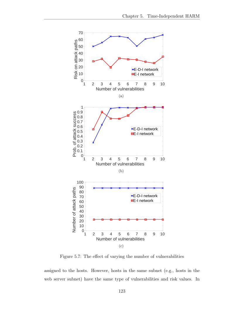
Chapter 5. Time-Independent HARM
1 2 3 4 5 6 7 8 9 10Number of vulnerabilities
0
10
20
30
40
50
60
70
Ris
k on
atta
ck p
aths
E-D-I networkE-I network
(a)
1 2 3 4 5 6 7 8 9 10Number of vulnerabilities
00.10.20.30.40.50.60.70.80.9
1
Pro
b. o
f atta
ck s
ucce
ss
E-D-I networkE-I network
(b)
1 2 3 4 5 6 7 8 9 10Number of vulnerabilities
0102030405060708090
100
Num
ber
of a
ttack
pat
hs
E-D-I networkE-I network
(c)
Figure 5.7: The effect of varying the number of vulnerabilities
assigned to the hosts. However, hosts in the same subnet (e.g., hosts in the
web server subnet) have the same type of vulnerabilities and risk values. In
123
Chapter 5. Time-Independent HARM
addition, the set of vulnerabilities found in network states for the same time
window (T) may vary because the vulnerabilities are randomly assigned.
Figure 5.7 shows the results. In Figures 5.7(a) and 5.7(b), the metrics
show similar effect. Here, regardless of the network model and number of
vulnerabilities found on hosts, the metrics show different values for the same
weight factor. However, in Figure 5.7(c), the metric did not change for all
time that vulnerabilities are added to the states. This is because a two-layer
security model is used, where attack paths are captures in the upper layer
and the vulnerabilities information is captured in the lower layer. Moreover,
since the network hosts already have one exploitable vulnerability each, that
has already created attack paths for the hosts in the upper layer. As a result,
adding more vulnerabilities on the hosts do not affect the number of possible
attack paths (because every attack path is already represented).
5.3.4 Computing the Minimal Weight Value to Use
Using high weight value may sometimes result in complete loss of attack
paths to the target hosts. This happens when connections (edges) from the
attacker to the target host are not the same connections in the network states
persistently (as a result of firewall rules changing, shuffle in MTD [73], users
disconnecting and joining, etc). Hence, it is important to find an approach to
determine the minimum weight threshold with non zero attack paths for the
TI-HARM. In this section, the proposed algorithm in Algorithm 6 is used to
compute the minimum weight value. Further, Figure 5.3 is used to explain the
results.
The networks and settings presented in Scenario I (Section 5.3.3) is used
for the simulations. Also, the simulation is run many times until a threshold
less than 0.4 is found (which is close to the ‘best’ threshold value), and the
step interval is set to 10 (here, a user can specify a desired threshold to allow).
The result of this simulation is presented in Table 5.7. Using the algorithm,
the minimum ‘safe’ weight value to use is w = 30.0% and w = 40.0% for E-D-I
124
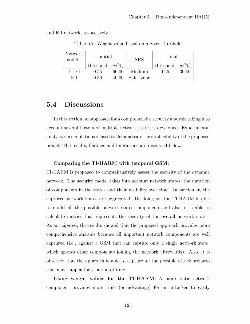
Chapter 5. Time-Independent HARM
and E-I network, respectively.
Table 5.7: Weight value based on a given threshold
Networkmodel
initialSRS
final
threshold w(%) threshold w(%)E-D-I 0.55 60.00 Medium 0.26 30.00E-I 0.36 40.00 Safer zone - -
5.4 Discussions
In this section, an approach for a comprehensive security analysis taking into
account several factors of multiple network states is developed. Experimental
analysis via simulations is used to demonstrate the applicability of the proposed
model. The results, findings and limitations are discussed below.
Comparing the TI-HARM with temporal GSM:
TI-HARM is proposed to comprehensively assess the security of the dynamic
network. The security model takes into account network states, the duration
of components in the states and their visibility over time. In particular, the
captured network states are aggregated. By doing so, the TI-HARM is able
to model all the possible network states components and also, it is able to
calculate metrics that represents the security of the overall network states.
As anticipated, the results showed that the proposed approach provides more
comprehensive analysis because all important network components are well
captured (i.e., against a GSM that can capture only a single network state,
which ignores other components joining the network afterwards). Also, it is
observed that the approach is able to capture all the possible attack scenario
that may happen for a period of time.
Using weight values for the TI-HARM: A more static network
component provides more time (or advantage) for an attacker to easily
125

Chapter 5. Time-Independent HARM
study and find potential system vulnerabilities, then exploit them in order
to penetrate through valuable network assets and steal sensitive information
[163]. These analysis results show that increasing the weight value in the
TI-HARM can generate a security model with the most persistent network
components. Thus, the TI-HARM can generate important components for
security assessments.
Security evaluations: The security analysis performed have shown that
several existing security metrics (e.g, system risk, the probability of attack
success) can be computed via TI-HARM. However, they may be some overhead
in the calculations of the metric for large size network when smaller weight value
(e.g., w = 0.0%) is used to construct the TI-HARM. So, there is a need to find a
method to reduce the overhead of using the smaller weight values in the future
work.
5.5 Summary
The properties of dynamic networks make it technically challenging to carry
out a security analysis, where there is a lack of methods and techniques to
capture different security posture when the network changes. In this chapter,
TI-HARM is developed to comprehensively model and analyse the security
of changing networks by taking into account multiple network states, their
duration and the visibility of components in the states. Further, the effect of
using different weight threshold to construct the TI-HARM is investigated.
Then, an algorithm for determining the MWT to use in order to prevent
misleading security analysis when using the TI-HARM is developed. The
analysis showed that TI-HARM could model and analyse the overall security
of changing networks which were not possible using existing GSM.
126

Chapter 6
Metrics for Assessing the
Security of Dynamic Networks
To get an accurate assessment of network security, security metrics are
necessary to quantify the level of the security. However, it is a challenging task
to quantify the security of modern networks due to the unpredictable network
and security posture changes at different times. Therefore, a systematic
approach is needed to quantitatively assess the security posture of dynamic
networks. There are many quantitative security metrics that are used with
traditional GSMs such as AG, to assess the security posture of the network
[2, 15, 19, 33, 48, 79, 108, 114, 127, 137]. However, these approaches assumed
the network of static nature. As such, changes made due to networking
functionalities (e.g., firewall rule change, host joining, host migration in the
cloud [37], etc.) changes the security posture and the security information,
which are not captured using the traditional GSMs and metrics.
In this chapter, T-HARM and TI-HARM are used to address the
aforementioned problems by developing a new set of security metrics to assess
the security of dynamic networks. First, all the possible security changes that
will be measured are identified (i.e., based on characteristics of the dynamic
network and their relations to system risk). Next, formulas are built to capture
every change in the network states under consideration. Furthermore, the
127
Chapter 6. Metrics for Assessing the Security of Dynamic Networks
security metrics are grouped according to their functionalities and what they
can capture or represent. Examples and simulations are used to demonstrate
the proposed security metrics. The main contributions in this chapter are
summarised as follows.
� Categorise the metrics for assessing the security of dynamic networks;
� Develop a new set of metrics to measure different aspects of the security
of dynamic networks;
� Demonstrate the applicability of the new security metrics.
6.1 Metrics for Assessing Dynamic Networks
There is a lack of approach to quantitatively assess the security of dynamic
networks [19]. As a result, two groups of security metrics for the analysis of
dynamic networks are developed; (1) Dynamic metrics (2) Stateless metrics.
The dynamic security metrics capture and assess the changing security posture
of networks when the network components change over time. On the other
hand, the stateless metrics provide the overview of the security posture of the
dynamic network for a given time window. Figure 6.1 shows the different groups
of the the metrics for the assessment of dynamic networks, and Section 6.1.1
(Dynamic metrics) and Section 6.1.2 (Stateless metrics) explains the different
groups. Since the proposed metrics are grouped and modularised, this approach
provides flexibility to add/modify/remove metrics as necessary.
6.1.1 Dynamic Metrics
Existing security metrics lack the capabilities to represent the changes in
the security posture of networks as the network components change over time.
It is of paramount importance to understand the changing security posture
in order to provide effective security solutions. To address this issue, attack
128

Chapter 6. Metrics for Assessing the Security of Dynamic Networks
Metrics to AssessDynamic Networks
Dynamic Metrics
AttackEfforts
(Figure 6.2)
DefenceEfforts
(Figure 6.3)
Stateless Metrics
VisibilityApproach
WeightedApproach
Risk
Path Number
Cost
...
Risk
...
Figure 6.1: Metrics for assessing dynamic networks
and defence efforts are taken into account to develop a set of new security
metrics to capture the effects security changes with respect to changes in the
network using the T-HARM. First, Section 6.1.1.4 presents the attack efforts
metrics, and Section 6.1.1.5 presents the defence efforts metrics. Lastly, the
quantification of these metrics is shown in Section 6.1.3. In the following, the
new dynamic security metrics are presented.
6.1.1.1 Attack and Defence Efforts Metrics
There are different efforts made by attackers and defenders depending on
the imposed threat to the system. The attack and defence efforts are presented
in this section, which is used to develop new security metrics for assessing
the security of dynamic networks. First, the attack efforts is classified in
Section 6.1.1.2, followed by the classification of defense efforts in Section 6.1.1.3.
129

Chapter 6. Metrics for Assessing the Security of Dynamic Networks
Attack Efforts
Reconnaissance
Scanning Frequency
Resource
Capability Time
· · ·
Path Number
Path Variation
...
Exposure
Cost
...
Knowledge
Tools
...
Duration
...
Figure 6.2: Categorising attack efforts
6.1.1.2 Categorisation of Attack Efforts
Attack efforts vary depending on the complexity of the attack scenario,
which is dependent on the security characteristics of the network configuration.
Hence, identifying security characteristics of the network configuration can
be used to evaluate the attack efforts. Here, the security characteristics of
dynamic networks are specify by the changes made in the network configuration
(see Table 3.2) which can be as a result of users’ activities (e.g., installations
of applications) or security administrator’ activities (e.g., apply defence
mechanisms), etc. Figure 6.2 shows the categorisation of attack efforts. It shows
two subcategories of the attack efforts, based on Reconnaissance and Resource.
Reconnaissance is an action taken by the attacker to gather information.
This is further divided into Scanning and Frequency, where Scanning observes
the network configurations, and Frequency specifies the amount of scanning.
Resource specifies the properties of the attacker, which divides into Capability
and Time. Capability specifies the ability of the attacker (e.g., knowledge
of attacks, tool availability, etc.), and Time specifies how much time would
be/has taken for the cyberattack. New dynamic security metrics are proposed
to capture those attack efforts in Section 6.1.1.4.
130
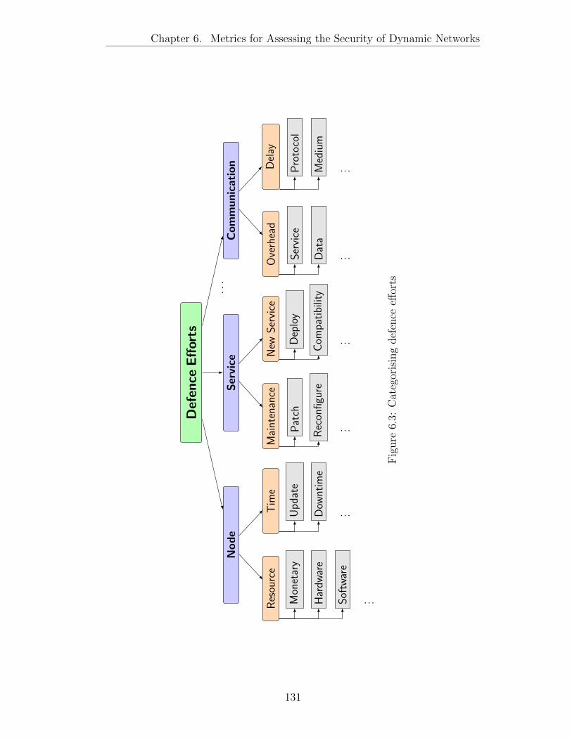
Chapter 6. Metrics for Assessing the Security of Dynamic Networks
Def
ence
Eff
ort
s
No
de
Res
ourc
eT
ime
Ser
vice
Mai
nten
ance
New
Ser
vice
Co
mm
un
ica
tio
n
Ove
rhea
dD
elay
···
Mon
etar
y
Har
dwar
e
Sof
twar
e
. . .
Up
date
Dow
ntim
e
. . .
Pat
ch
Rec
onfi
gure
. . .
Dep
loy
Com
pati
bilit
y
. . .
Ser
vice
Dat
a
. . .
Pro
toco
l
Med
ium
. . .
Fig
ure
6.3:
Cat
egor
isin
gdef
ence
effor
ts
131
Chapter 6. Metrics for Assessing the Security of Dynamic Networks
6.1.1.3 Categorisation of Defence Efforts
The deployment of security measures on the network changes the security
posture as well. As a result, the security administrator needs to consider the
cost that is associated with such a deployment. The defender’s efforts made
when deploying security measure for modern networks is considered. Figure 6.3
shows the categorisation of defence efforts. It shows three subcategories on the
basis of network components; network nodes, services, and communications.
The deployment of security measures (e.g., security update) can change the
security information of Nodes (e.g., hosts), and besides this require time and
resources to do so. Services form a platform for interaction (e.g., applications),
which requires the adoption and deployment of new services and maintenance.
This can be changed using some security measures such as hosts migration.
Communications (e.g., connections between network nodes) can be changed by
modifying the firewall rules, etc. Similarly, with attack efforts, new dynamic
security metrics capturing each subcategory of defence efforts are presented in
Section 6.1.1.5.
6.1.1.4 Attack Efforts Metrics
This security metrics aim to capture the change in security posture as the
network configurations and attack vector changes. One aspect of the attack
vector is the attack paths. By observing the changes to attack paths, the
increase in the attack effort can be evaluated.
Scanning: Path Number
This metric is used to show the exposure of the dynamic network states
to attack. The network security can negatively be affected when there is an
increasing number of attack paths, as it reveals more choices to be taken by the
attacker when the scanning is carried out. Therefore, changes in the number
of attack paths when network changes occur need to be taken into account
132
Chapter 6. Metrics for Assessing the Security of Dynamic Networks
in order to understand the changes in the security of the network in terms
of possible paths to reach the target. Equation (6.1) shows the proportion of
attack paths increased. If the number of attack paths stays the same, then it
equates to value 0. However, if the previous network state had no attack paths,
then it equates to 1.
|APnsti | − |APnsti−1|
|APnsti |(6.1)
Now consider a reduced number of attack paths in the current network state.
Assuming that the attack efforts stay the same (i.e., there is no advantage),
then the security metric can be calculated as shown in equation (6.2).
max(|APnsti | − |APnsti−1|, 0)
|APnsti |(6.2)
The difference between the number of attack paths for all network states is
computed and then normalised. Equation (6.3) shows the computation of APN
metric that measures the differences between the numbers of attack paths for
all network states. The APN metric does not need an arbitrary assignment of
values, and it is calculated only based on the observed number of attack paths
from all network states NS.
APN =
∑|NS|i=1
max(|APnsti |−|APnsti−1|,0)
|APnsti |
|NS| − 1(6.3)
Frequency: Exposure
The duration of attack path exposure for dynamic networks can be
calculated. It is assumed that the attacker is likely to prepare and launch
an attack successfully if the exposure of an attack path is long enough (e.g.,
133

Chapter 6. Metrics for Assessing the Security of Dynamic Networks
the attack lifetime described in [53]). Hence, the duration of an attack path
should be minimised to enhance security. However, estimating the amount of
time needed for the attacker to prepare and launch an attack is difficult. Hence,
the best case is to minimise the duration of an attack path exposure. That is,
the goal of the metric is to compute the duration of each attack path exposed.
The function t(api) is used to compute the attack path exposure as shown in
equation (6.4), which is normalised by the number of attack paths and the total
number of network states.
APE =
∑|NS|i=0 t(apj)
|AP | ×∑|NS|
i=1 t(nsti)∀apj ∈ APnsti (6.4)
For the APE metric, if the initial set of attack paths are exposed in all the
network states without any new attack paths, then the APE value tends toward
one. Hence, it is better to achieve a lower value of APE which represents that
an attack path is only exposed in one network state.
Capability: Knowledge
Costs are one of the important decision constraints for both attackers and
defenders. Here, the cost of an attack is estimated based on the difficulty
of exploiting vulnerabilities using the CVSS, particularly the exploitability
score (from the Base Equation of the CVSS) that determines the difficulty of
exploiting the vulnerability (i.e., the knowledge of the attacker will determine
the ability to exploit vulnerabilities with lower exploitability scores etc). The
CVSS version 2 is used, as many of the legacy vulnerabilities do not have
version 3 available yet, but new vulnerabilities still have version 2 available,
which is more practical (both versions have the exploitability (sub) score which
is used in this subsection). However, other means of cost metrics can be used
to further categorise the knowledge category of the attacker efforts in addition
to the CVSS exploitability scores.
134
Chapter 6. Metrics for Assessing the Security of Dynamic Networks
The attack cost associated with exploiting vulnerability can be calculated
by taking into account all possible attack paths. Then, the exploitability of each
attack path becomes the cumulative product of all the vulnerabilities required.
The attack cost of exploitation for a state, ACnsti , is shown in equation (6.5).
ACnsti =
|APnsti |∏j=1
(1−
|apj |∏k=1
Ep(vk))
,where vk ∈ vuls(apj)∀apj ∈ APi
(6.5)
Using the above equation, the attack cost associated with the exploitation of
vulnerabilities can be computed as shown in equation (6.6) taking into account
all network states.
ACE =
∑|NS|i=0 ACnsti|NS|
(6.6)
The inner product computes the exploitability of each attack path and
combines them using the disjoint set theory. This is processed for all network
states.
Time: Duration
The amount of time taken for the attacker to compromise each stepping
stone in an attack path is another significant factor, as the longer the attack
takes, the more likely it will be detected. Hence, increasing the amount of
time to attack can negatively affect the attacker. Also, it is assumed that
the attacker will minimise the time taken for an attack. Hence, the minimum
time taken by the attacker to compromise the target in each network state is
computed based on the time taken to exploit each vulnerability in the attack
path, which is presented as a function t(api). In practice, the minimum time
to exploit can be approximated (i.e., the function t(apj)) through empirical
135
Chapter 6. Metrics for Assessing the Security of Dynamic Networks
studies [112], as well as using other timing models as appropriate. Assuming
that exploiting a vulnerability has a specific time frame, then there is no need
to consider the skills of different attackers. Equation (6.7) shows the normalised
metric representing the time taken to compromise the target in a given network
state. The time has been normalised by the maximum amount of time to
compromise the target by the attacker.
ACD =
|NS|∑i=0
min(t(apj))
max(t(apj))
|NS|∀apj ∈ APnsti (6.7)
The ACD metric computes the ratio of the shortest and longest times taken
for the attacker to exploit the target in each network state. Hence, higher
ACD value represents that a significant proportion of the network states can
be exploited in a shorter time than the expected maximum amount of time.
6.1.1.5 Defence Efforts Metrics
There are different type of costs associated with deploying security
hardening measures in the network. In this section, the cost associated with
defence efforts are captured and presented in Section 6.1.1.3.
Time: Implementation Downtime
The implementation of a security measure causes a downtime in the
network. The aim of this metric is to show the downtime experience as a result
of the implementations of security measures. Downtimes can be estimated
and measured, which can be used for input to this metric calculations. First,
equation (6.8) shows the downtime, calculation of a given network state nsi.
max(dt(cmk, hj)),∀hj ∈ Hi (6.8)
136
Chapter 6. Metrics for Assessing the Security of Dynamic Networks
Equation (6.9) shows the downtime experienced when implementing
security measures for dynamic networks. The downtime has been normalised
by the maximum downtime experienced.
NDT =
|NS|∑i=1
max(dt(cmk, hj))
|NS| ×max(dt(cmk, hj))
∀hj ∈ Hi,∀cmk ∈ CM
(6.9)
The higher NDT value represents more downtime observed when
implementing the defence measures in the network. As the NDT value
converges to zero, it represents the minimum downtime for all network states.
Overhead: Service
As a form of defence mechanism, the network topology can be reconfigured
to improve security. However, there is a cost associated with maintaining
communication (i.e., edges) between the network components. Such costs
depend on which communication service is in use, and how the communication
paths are changed. For the basics, the difference between the edge set is defined
as the edge changing cost (ECC). Assuming that the cost of changing the
edge is the same. Then, it is only the number of edge changes between the
network states that will be counted. Networking technologies deploy edge
changes in parallel (e.g., SDN) but the amount of change still affects the
network performance of the affected region. Hence, the more edge changes,
the higher cost is observed (e.g., delay or downtime). The edge variation cost
can be computed as shown in equation (6.10), where the cost of each network
state is normalised by the maximum edge variation cost, and the total cost
137
Chapter 6. Metrics for Assessing the Security of Dynamic Networks
normalised by the number of network states.
ECC =
|NS|∑i=1
|et(nsti )et(nsti−1 )||et(nsti )∪et(nsti−1 )|
|NS| − 1(6.10)
Delay: Medium
Defence mechanisms such as traffic redirection, host isolations, shuffle
in moving target defences [73], etc. involves the changing/removing the
connections between hosts. This event may attracts a delay and loss of data
between the communications (similar to the downtime of implementation under
Node category). Hence, it is important that such defence mechanisms do
not affect the system performance by limiting the edge changing time. The
equation (6.11) shows the computation of the time duration of the edge pair
changes in nsti .
et(nsti) = max(et(hj)∀hj ∈ Hi) (6.11)
Given the time duration of the edge pair changes, the edge variation time
can be calculated for all network states as shown in equation (6.12). The
edge variation time is normalised by the maximum amount of time taken for
changing the edge sets.
ECT =
∑|NS|i=1 et(nsti)
max(et(nsti))× (|NS| − 1),∀nsti ∈ NS (6.12)
6.1.2 Stateless Metrics
The stateless security risk assessment provides network state-independent
view of the security. That is, the security metric value calculated represents all
the observed network states.
138
Chapter 6. Metrics for Assessing the Security of Dynamic Networks
Two main approaches are used: 1) Visibility Approach (VA), and 2)
Weighted Approach (WA). The VA approach combines all the observed network
configurations onto a single GSM and then calculates a metric which represents
the states. The TI-HARM can be used to calculate the metrics for the VA.
In contrast, the WA approach evaluates the security of each network state and
then combines them based on their time duration converted into weights (i.e.,
the proportion of the network state visibility).
6.1.2.1 Visibility Aggregation
The VA approach collects all visible network states. This approach enables
one to capture all the network states information in the security assessment
and maintain the same security assessment as long as the observed states are
not changed. The limitation of the VA approach is that it does not reflect the
exposure of different network states (i.e., the time information is not taken into
account).
VA: Path Number
The ultimate goal of this metric is to quantitatively represent the number of
ways an attacker can use the existing security weakness (i.e., vulnerabilities and
their relationship) to compromise a network system over a period of time. This
metric shows the total number of attack paths that are visible for a period
of time. Thus, a high number of attack paths reveals more choices to be
taken by the attacker when the scanning is carried out. Here, the network
administrator’s task is to minimally reduce the number of attack paths for all
the states. Equation (6.13) shows the set of attack paths for a network state
nsti .
APnsti = {ap0, ap1, ap2, ..., apn} (6.13)
139
Chapter 6. Metrics for Assessing the Security of Dynamic Networks
Then the unique number of attack paths for the network states can be
calculated by equation (6.14).
V A : APN = |APnst0 ∪ APnst1 ∪ APnst2 ∪ ... ∪ APnstn | (6.14)
VA: Persistent Attack Paths Number
The goal of the metric is to calculate the weakest part of a dynamic network
in terms of the set of attack paths that appear in all the states. Typically, this
set of attack paths will provide the attacker more time to plan a successful
attack on the network hosts. Moreover, some defence mechanisms are not able
to remove all attack paths, and as a result, the security administrator needs to
identify the persistent attack paths for other forms of defence. In this regard,
the number of the most persistent attack paths are captured over a period of
time using this metric. First, the set of attack paths for each network states
can be captured by using equation (6.15).
APnsti = {ap0, ap1, ap2, ..., apn} (6.15)
The set intersection of all the states attack paths will capture the persistent
paths for the time window in consideration. So, the calculations for the
Persistent Attack Paths Number (PAP) is giving by equation (6.16).
V A : PAP = |APnst0 ∩ APnst1 ∩ APnst2 ∩ ... ∩ APnstn | (6.16)
VA: Security Stateless Risk
This metric calculates the overall security of the network states by
aggregating all the observed components in the states. However, it does not
take into account the time duration of the network states. The VA stateless
140
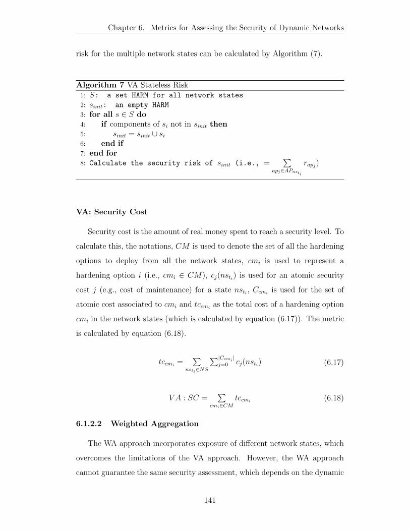
Chapter 6. Metrics for Assessing the Security of Dynamic Networks
risk for the multiple network states can be calculated by Algorithm (7).
Algorithm 7 VA Stateless Risk1: S: a set HARM for all network states
2: sinit: an empty HARM
3: for all s ∈ S do4: if components of si not in sinit then5: sinit = sinit ∪ si6: end if7: end for8: Calculate the security risk of sinit (i.e., =
∑apj∈APnsti
rapj)
VA: Security Cost
Security cost is the amount of real money spent to reach a security level. To
calculate this, the notations, CM is used to denote the set of all the hardening
options to deploy from all the network states, cmi is used to represent a
hardening option i (i.e., cmi ∈ CM), cj(nsti) is used for an atomic security
cost j (e.g., cost of maintenance) for a state nsti , Ccmi is used for the set of
atomic cost associated to cmi and tccmi as the total cost of a hardening option
cmi in the network states (which is calculated by equation (6.17)). The metric
is calculated by equation (6.18).
tccmi =∑
nsti∈NS
∑|Ccmi |j=0 cj(nsti) (6.17)
V A : SC =∑
cmi∈CMtccmi (6.18)
6.1.2.2 Weighted Aggregation
The WA approach incorporates exposure of different network states, which
overcomes the limitations of the VA approach. However, the WA approach
cannot guarantee the same security assessment, which depends on the dynamic
141

Chapter 6. Metrics for Assessing the Security of Dynamic Networks
behaviour of the network. Moreover, it requires more computational resources
due to the security assessment of each network state, compared to the VA
approach.
WA: Security Stateless Risk
This metric uses the hosts (nodes) risk value (e.g., from CVSS BS) to
calculate the metric at the attack path level, to network state level and then the
overall risk for the time duration. The attack path level risk rapi is calculated
by equation (6.19), the network state risk by equation (6.20), and the WA
stateless risk is calculated by equation (6.21).
rapj =∑
hti∈apiprhti × aimhti
, api ∈ APnsti (6.19)
Rnsti=
∑apj∈APnsti
rapj (6.20)
V A : SR =∑
nsti∈NS
(Rnsti
× t(nsti )
T
)(6.21)
6.1.3 Application of Dynamic Security Metric Modules
This section describes the use of the proposed metrics using an example
dynamic network. The network and the attacker model are shown in
Section 3.2. The reachability of the hosts, the metrics associated to the hosts
are shown in Figure 6.4, Table 6.1 and Table 6.2 (and Table 6.3 as well), and the
network topologies are shown in in Figure 6.4. Time is assigned to the network
topologies, the number of hours is chosen arbitrarily for demonstration only, the
actual duration of each network state can be measured based on reconfiguration
schedules. The attack goal is to reach the target host DB through an elevation
of privilege. Assuming that each host has a remote-to-root vulnerability, and
different operating systems have different exploitability values, the time is taken
142
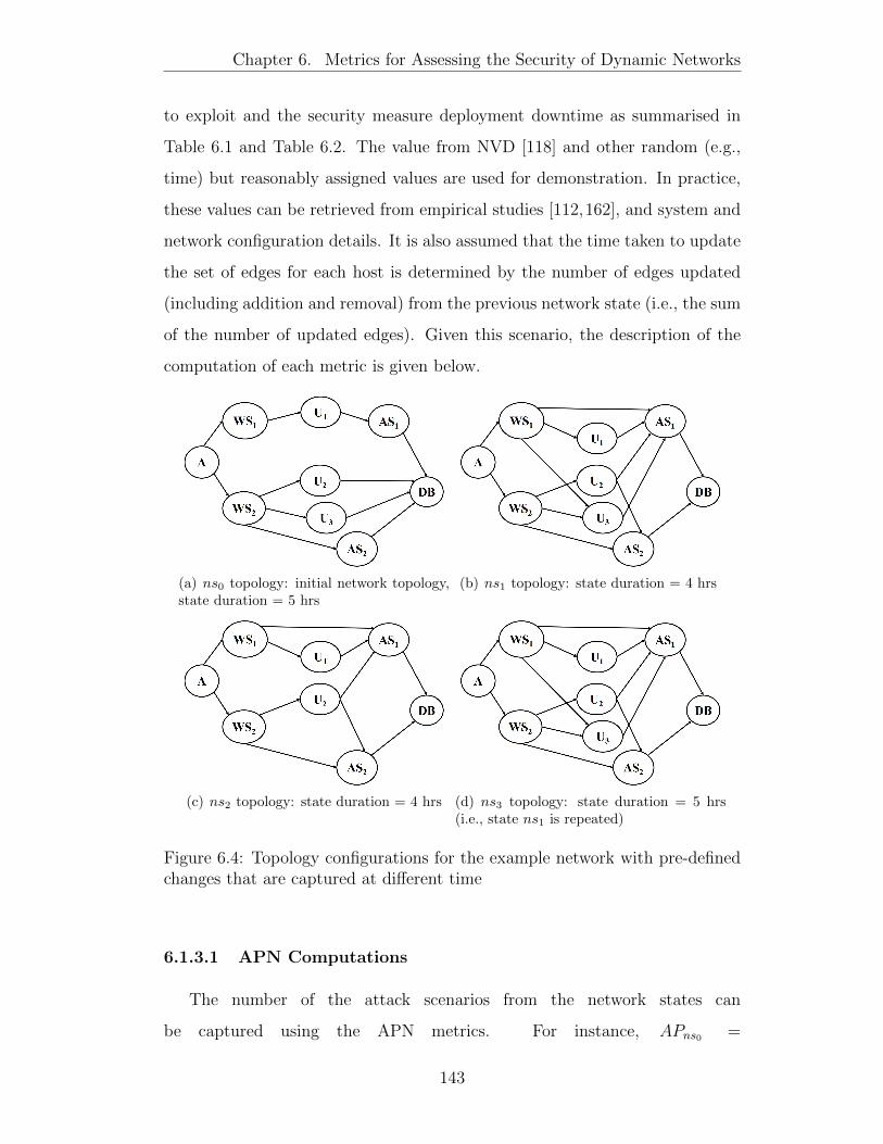
Chapter 6. Metrics for Assessing the Security of Dynamic Networks
to exploit and the security measure deployment downtime as summarised in
Table 6.1 and Table 6.2. The value from NVD [118] and other random (e.g.,
time) but reasonably assigned values are used for demonstration. In practice,
these values can be retrieved from empirical studies [112,162], and system and
network configuration details. It is also assumed that the time taken to update
the set of edges for each host is determined by the number of edges updated
(including addition and removal) from the previous network state (i.e., the sum
of the number of updated edges). Given this scenario, the description of the
computation of each metric is given below.
(a) ns0 topology: initial network topology,state duration = 5 hrs
(b) ns1 topology: state duration = 4 hrs
(c) ns2 topology: state duration = 4 hrs (d) ns3 topology: state duration = 5 hrs(i.e., state ns1 is repeated)
Figure 6.4: Topology configurations for the example network with pre-definedchanges that are captured at different time
6.1.3.1 APN Computations
The number of the attack scenarios from the network states can
be captured using the APN metrics. For instance, APns0 =
143
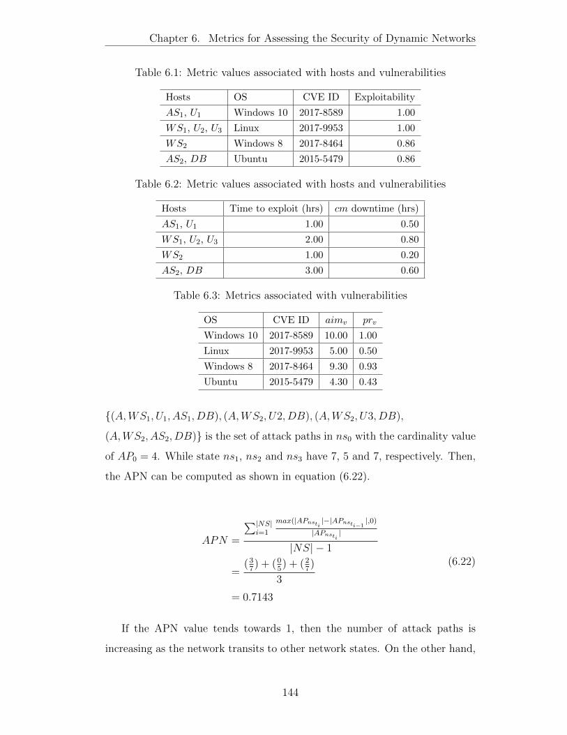
Chapter 6. Metrics for Assessing the Security of Dynamic Networks
Table 6.1: Metric values associated with hosts and vulnerabilities
Hosts OS CVE ID Exploitability
AS1, U1 Windows 10 2017-8589 1.00
WS1, U2, U3 Linux 2017-9953 1.00
WS2 Windows 8 2017-8464 0.86
AS2, DB Ubuntu 2015-5479 0.86
Table 6.2: Metric values associated with hosts and vulnerabilities
Hosts Time to exploit (hrs) cm downtime (hrs)
AS1, U1 1.00 0.50
WS1, U2, U3 2.00 0.80
WS2 1.00 0.20
AS2, DB 3.00 0.60
Table 6.3: Metrics associated with vulnerabilities
OS CVE ID aimv prv
Windows 10 2017-8589 10.00 1.00
Linux 2017-9953 5.00 0.50
Windows 8 2017-8464 9.30 0.93
Ubuntu 2015-5479 4.30 0.43
{(A,WS1, U1, AS1, DB), (A,WS2, U2, DB), (A,WS2, U3, DB),
(A,WS2, AS2, DB)} is the set of attack paths in ns0 with the cardinality value
of AP0 = 4. While state ns1, ns2 and ns3 have 7, 5 and 7, respectively. Then,
the APN can be computed as shown in equation (6.22).
APN =
∑|NS|i=1
max(|APnsti |−|APnsti−1|,0)
|APnsti |
|NS| − 1
=(37) + (0
5) + (2
7)
3
= 0.7143
(6.22)
If the APN value tends towards 1, then the number of attack paths is
increasing as the network transits to other network states. On the other hand,
144
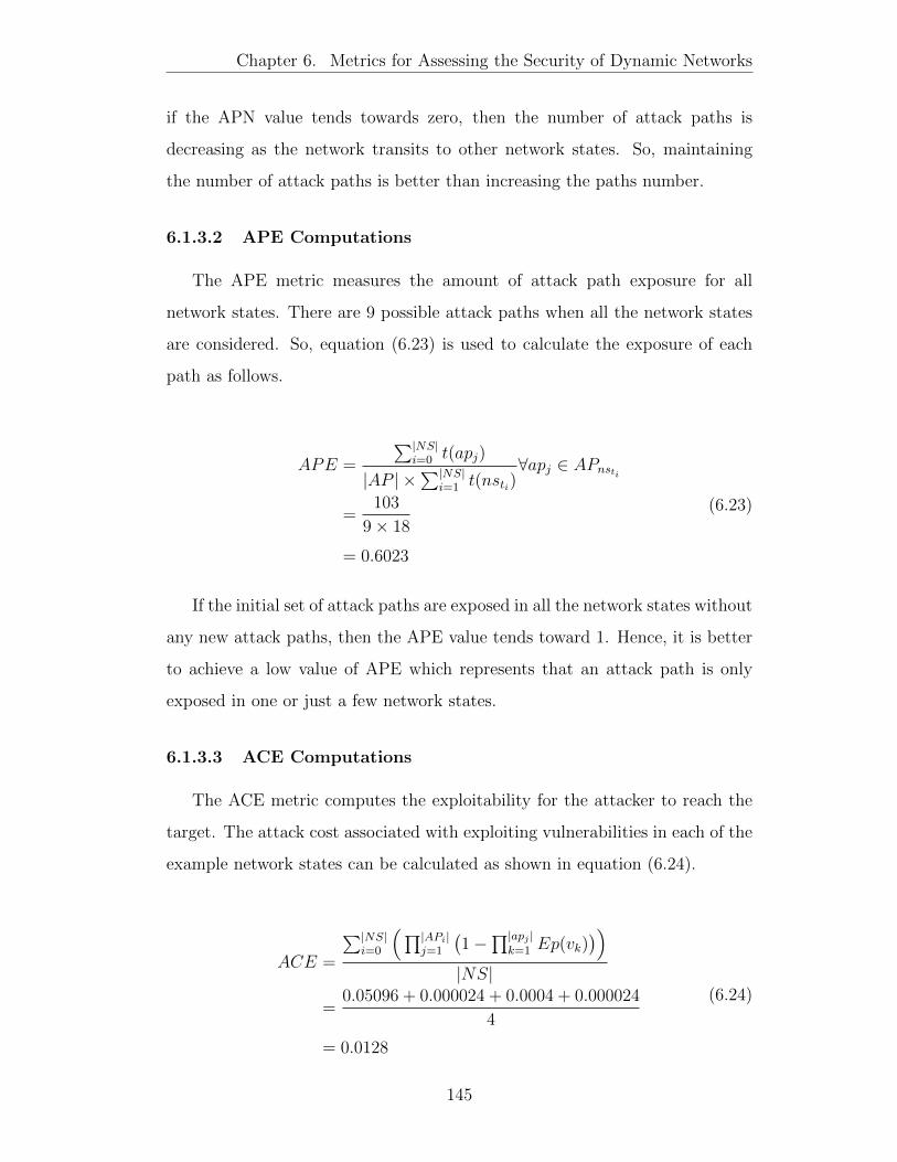
Chapter 6. Metrics for Assessing the Security of Dynamic Networks
if the APN value tends towards zero, then the number of attack paths is
decreasing as the network transits to other network states. So, maintaining
the number of attack paths is better than increasing the paths number.
6.1.3.2 APE Computations
The APE metric measures the amount of attack path exposure for all
network states. There are 9 possible attack paths when all the network states
are considered. So, equation (6.23) is used to calculate the exposure of each
path as follows.
APE =
∑|NS|i=0 t(apj)
|AP | ×∑|NS|
i=1 t(nsti)∀apj ∈ APnsti
=103
9× 18
= 0.6023
(6.23)
If the initial set of attack paths are exposed in all the network states without
any new attack paths, then the APE value tends toward 1. Hence, it is better
to achieve a low value of APE which represents that an attack path is only
exposed in one or just a few network states.
6.1.3.3 ACE Computations
The ACE metric computes the exploitability for the attacker to reach the
target. The attack cost associated with exploiting vulnerabilities in each of the
example network states can be calculated as shown in equation (6.24).
ACE =
∑|NS|i=0
(∏|APi|j=1
(1−
∏|apj |k=1 Ep(vk)
))|NS|
=0.05096 + 0.000024 + 0.0004 + 0.000024
4
= 0.0128
(6.24)
145
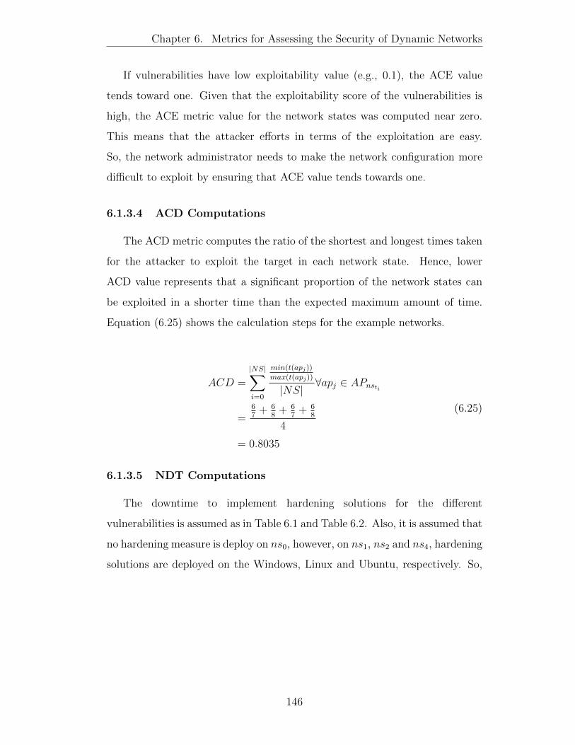
Chapter 6. Metrics for Assessing the Security of Dynamic Networks
If vulnerabilities have low exploitability value (e.g., 0.1), the ACE value
tends toward one. Given that the exploitability score of the vulnerabilities is
high, the ACE metric value for the network states was computed near zero.
This means that the attacker efforts in terms of the exploitation are easy.
So, the network administrator needs to make the network configuration more
difficult to exploit by ensuring that ACE value tends towards one.
6.1.3.4 ACD Computations
The ACD metric computes the ratio of the shortest and longest times taken
for the attacker to exploit the target in each network state. Hence, lower
ACD value represents that a significant proportion of the network states can
be exploited in a shorter time than the expected maximum amount of time.
Equation (6.25) shows the calculation steps for the example networks.
ACD =
|NS|∑i=0
min(t(apj))
max(t(apj))
|NS|∀apj ∈ APnsti
=67
+ 68
+ 67
+ 68
4
= 0.8035
(6.25)
6.1.3.5 NDT Computations
The downtime to implement hardening solutions for the different
vulnerabilities is assumed as in Table 6.1 and Table 6.2. Also, it is assumed that
no hardening measure is deploy on ns0, however, on ns1, ns2 and ns4, hardening
solutions are deployed on the Windows, Linux and Ubuntu, respectively. So,
146

Chapter 6. Metrics for Assessing the Security of Dynamic Networks
the NDT can be calculated as shown in equation (6.26).
NDT =
|NS|∑i=1
max(dt(cmk, hj))
|NS| ×max(dt(cmk, hj)),∀hj ∈ Hi,∀cmk ∈ CM
=0
4× 0.8+
0.5
4× 0.8+
0.8
4× 0.8+
0.6
4× 0.8
= 0.5937
(6.26)
The higher NDT value represents more downtime observed when deploying
the security measures in the network. As the NDT value converges to one, it
represents the maximum downtime for all network states.
6.1.3.6 ECC Computations
If ns0 is assumed to be the initial network states, and the states ns1, ns2
and ns3 have been reconfigured (as it is presented) over time. Then the ECC
for the example network can be calculated by equation (6.27). The lower value
represents fewer changes to the set of edges between the network states.
ECC =
|NS|∑i=1
|et(nsti )et(nsti−1 )||et(nsti )∪et(nsti−1 )|
|NS| − 1
=79
+ 27
+ 27
3
= 0.4497
(6.27)
6.1.3.7 ECT Computations
The EVT measures the time taken to assign the edge sets in the network
state, which determines the delay observed in the network. The time taken
to update the edge pairs of a host is assumed to be the number of updated
edges. Then, the ECT calculation for the example network is as shown in
147
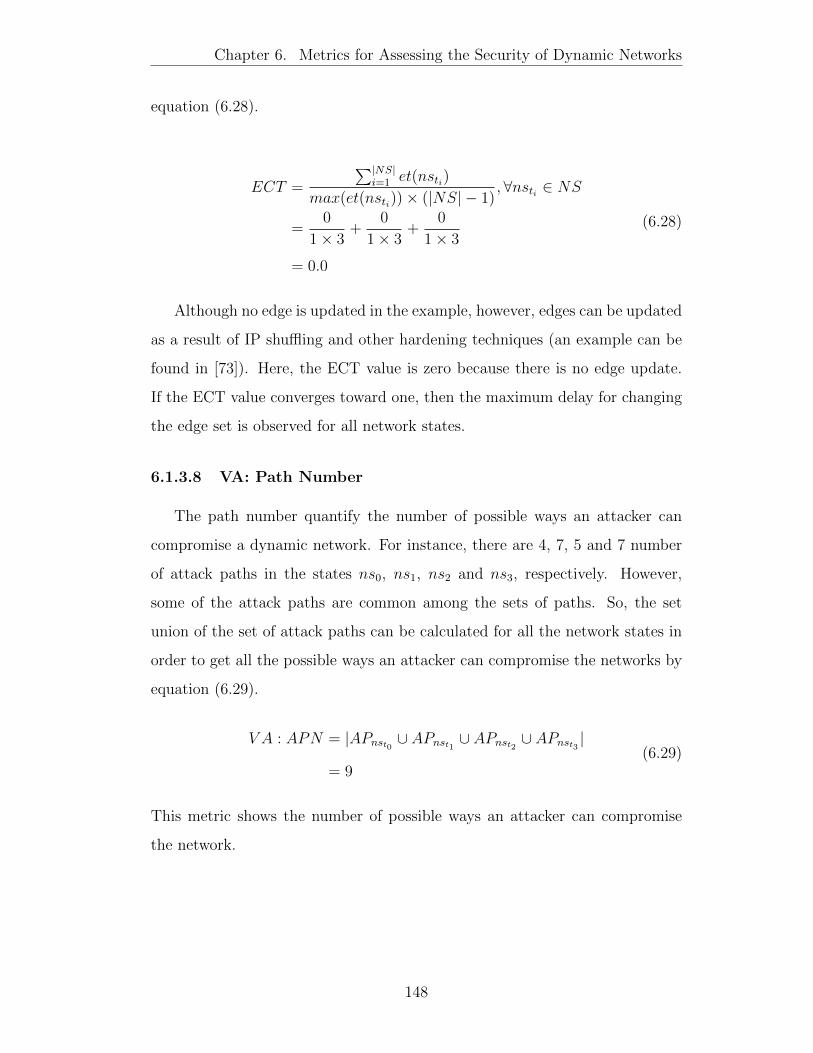
Chapter 6. Metrics for Assessing the Security of Dynamic Networks
equation (6.28).
ECT =
∑|NS|i=1 et(nsti)
max(et(nsti))× (|NS| − 1),∀nsti ∈ NS
=0
1× 3+
0
1× 3+
0
1× 3
= 0.0
(6.28)
Although no edge is updated in the example, however, edges can be updated
as a result of IP shuffling and other hardening techniques (an example can be
found in [73]). Here, the ECT value is zero because there is no edge update.
If the ECT value converges toward one, then the maximum delay for changing
the edge set is observed for all network states.
6.1.3.8 VA: Path Number
The path number quantify the number of possible ways an attacker can
compromise a dynamic network. For instance, there are 4, 7, 5 and 7 number
of attack paths in the states ns0, ns1, ns2 and ns3, respectively. However,
some of the attack paths are common among the sets of paths. So, the set
union of the set of attack paths can be calculated for all the network states in
order to get all the possible ways an attacker can compromise the networks by
equation (6.29).
V A : APN = |APnst0 ∪ APnst1 ∪ APnst2 ∪ APnst3 |
= 9(6.29)
This metric shows the number of possible ways an attacker can compromise
the network.
148

Chapter 6. Metrics for Assessing the Security of Dynamic Networks
6.1.3.9 VA: Persistent Attack Paths Number
The metrics capture the attack paths that appear in all the network states.
Here, The set intersection of all the states’ attack paths will capture the
persistent paths for the time window under consideration. So, the calculations
for the PAP is giving by equation (6.30).
V A : PAP = |APnst0 ∩ APnst1 ∩ APnst2 ∩ APnst3 |
= |{(A,WS1, U1, AS1, DB), (A,WS2, AS2, DB)}|
= 2
(6.30)
6.1.3.10 WA: Security Stateless Risk
The WA security stateless risk metric overcome the limitations of the VA
stateless risk by taking into account time duration of the network states. The
WA stateless risk for the example network can be calculated by equation (6.31)
as follows.
WA : SR =∑
nsti∈NS
(Rnsti
× t(nsti )
T
)=(
62.676× 518
)+(
128.737× 418
)+(
88.89× 418
)+(
128.737× 518
)= 101.5317
(6.31)
6.2 Simulations and Results
Experimental analysis via simulations is conducted to demonstrate the
functionalities of the proposed metrics based on attack effort metrics, defence
efforts and stateless security metrics. To generalise the proposed approach, a
generic dynamic network that randomly connects the hosts, which includes any
possible network configurations is used. By doing so, the subset of practical
network configurations is included in the analysis. Three factors are considered
149
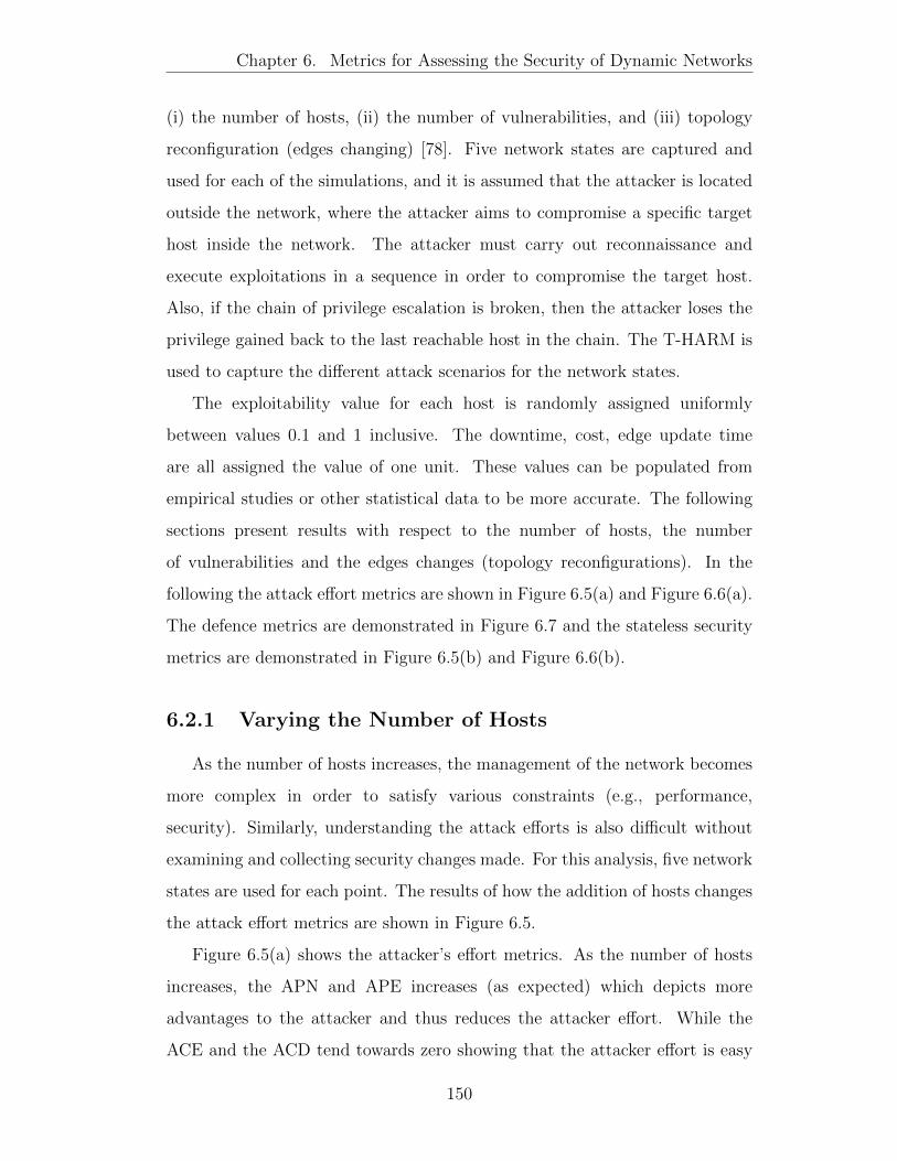
Chapter 6. Metrics for Assessing the Security of Dynamic Networks
(i) the number of hosts, (ii) the number of vulnerabilities, and (iii) topology
reconfiguration (edges changing) [78]. Five network states are captured and
used for each of the simulations, and it is assumed that the attacker is located
outside the network, where the attacker aims to compromise a specific target
host inside the network. The attacker must carry out reconnaissance and
execute exploitations in a sequence in order to compromise the target host.
Also, if the chain of privilege escalation is broken, then the attacker loses the
privilege gained back to the last reachable host in the chain. The T-HARM is
used to capture the different attack scenarios for the network states.
The exploitability value for each host is randomly assigned uniformly
between values 0.1 and 1 inclusive. The downtime, cost, edge update time
are all assigned the value of one unit. These values can be populated from
empirical studies or other statistical data to be more accurate. The following
sections present results with respect to the number of hosts, the number
of vulnerabilities and the edges changes (topology reconfigurations). In the
following the attack effort metrics are shown in Figure 6.5(a) and Figure 6.6(a).
The defence metrics are demonstrated in Figure 6.7 and the stateless security
metrics are demonstrated in Figure 6.5(b) and Figure 6.6(b).
6.2.1 Varying the Number of Hosts
As the number of hosts increases, the management of the network becomes
more complex in order to satisfy various constraints (e.g., performance,
security). Similarly, understanding the attack efforts is also difficult without
examining and collecting security changes made. For this analysis, five network
states are used for each point. The results of how the addition of hosts changes
the attack effort metrics are shown in Figure 6.5.
Figure 6.5(a) shows the attacker’s effort metrics. As the number of hosts
increases, the APN and APE increases (as expected) which depicts more
advantages to the attacker and thus reduces the attacker effort. While the
ACE and the ACD tend towards zero showing that the attacker effort is easy
150
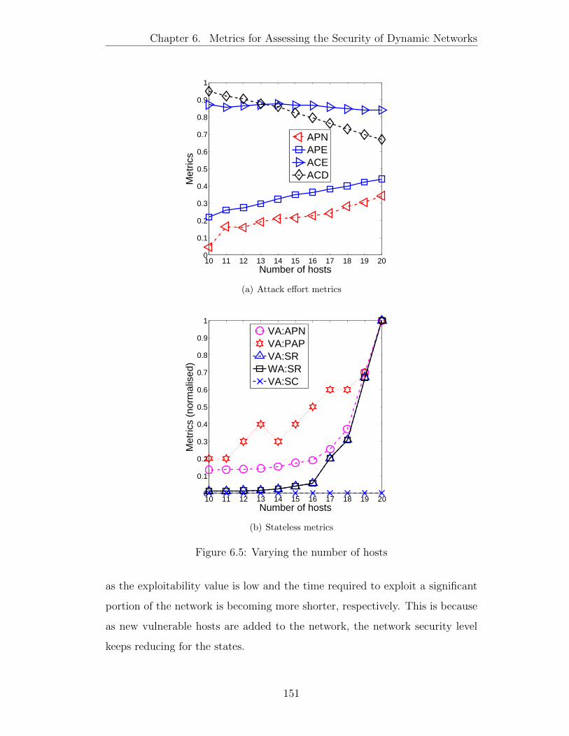
Chapter 6. Metrics for Assessing the Security of Dynamic Networks
10 11 12 13 14 15 16 17 18 19 200
0.1
0.2
0.3
0.4
0.5
0.6
0.7
0.8
0.9
1
Number of hosts
Met
rics
APNAPEACEACD
(a) Attack effort metrics
10 11 12 13 14 15 16 17 18 19 200
0.1
0.2
0.3
0.4
0.5
0.6
0.7
0.8
0.9
1
Number of hosts
Met
rics
(nor
mal
ised
)
VA:APNVA:PAPVA:SRWA:SRVA:SC
(b) Stateless metrics
Figure 6.5: Varying the number of hosts
as the exploitability value is low and the time required to exploit a significant
portion of the network is becoming more shorter, respectively. This is because
as new vulnerable hosts are added to the network, the network security level
keeps reducing for the states.
151
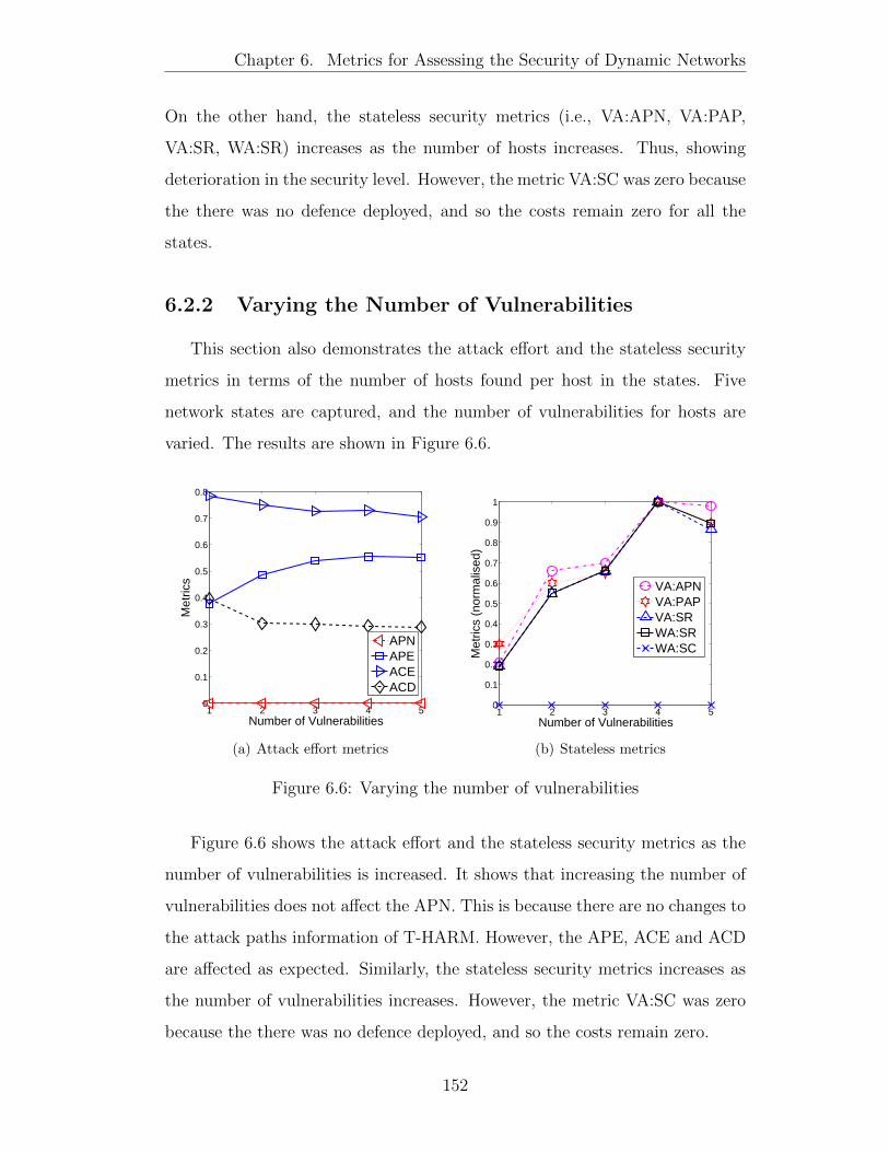
Chapter 6. Metrics for Assessing the Security of Dynamic Networks
On the other hand, the stateless security metrics (i.e., VA:APN, VA:PAP,
VA:SR, WA:SR) increases as the number of hosts increases. Thus, showing
deterioration in the security level. However, the metric VA:SC was zero because
the there was no defence deployed, and so the costs remain zero for all the
states.
6.2.2 Varying the Number of Vulnerabilities
This section also demonstrates the attack effort and the stateless security
metrics in terms of the number of hosts found per host in the states. Five
network states are captured, and the number of vulnerabilities for hosts are
varied. The results are shown in Figure 6.6.
1 2 3 4 50
0.1
0.2
0.3
0.4
0.5
0.6
0.7
0.8
Number of Vulnerabilities
Met
rics
APNAPEACEACD
(a) Attack effort metrics
1 2 3 4 50
0.1
0.2
0.3
0.4
0.5
0.6
0.7
0.8
0.9
1
Number of Vulnerabilities
Met
rics
(nor
mal
ised
)
VA:APNVA:PAPVA:SRWA:SRWA:SC
(b) Stateless metrics
Figure 6.6: Varying the number of vulnerabilities
Figure 6.6 shows the attack effort and the stateless security metrics as the
number of vulnerabilities is increased. It shows that increasing the number of
vulnerabilities does not affect the APN. This is because there are no changes to
the attack paths information of T-HARM. However, the APE, ACE and ACD
are affected as expected. Similarly, the stateless security metrics increases as
the number of vulnerabilities increases. However, the metric VA:SC was zero
because the there was no defence deployed, and so the costs remain zero.
152
Chapter 6. Metrics for Assessing the Security of Dynamic Networks
6.2.3 Changing Edges (Topology)
Network topology can be reconfigured or edges changed in order to provide
security. In this section, the optimal reconfiguration approach in [78] was
adopted and used as the network hardening. The approach in the paper
provides a method to optimally change the hosts’ edges. In order to
demonstrate the effects of changing the edges on the metrics, simulations are
performed with 20 hosts and fives dynamic states. The results are shown in
Figure 6.7. Figure 6.7 shows the defence efforts metrics. The results showed
10 11 12 13 14 15 16 17 18 19 200
0.1
0.2
0.3
0.4
0.5
0.6
0.7
0.8
0.9
1
Number of hosts
Met
rics
NDTECCECT
Figure 6.7: Defence Effort: Changing edges
that as the number of hosts increases, the defence effort increases as well. This
is showing that there are more edges needed to be changed to satisfy the security
goal and thus the increase in the metrics, as there are more hosts considered.
6.3 Summary
This chapter presented two group of security metrics to assess the security
of dynamic networks quantitatively. Examples and simulations are used to
demonstrate the usability of the proposed set of security metrics. The analysis
153

Chapter 6. Metrics for Assessing the Security of Dynamic Networks
results show the in-depth security changes of dynamic metrics and thus provide
an approach to quantify the security of networks that are changing in their
configurations.
154
Chapter 7
Security Hardening
Optimisation for Dynamic
Networks
Hardening the dynamic networks is a very challenging task due to their
complexity and dynamicity. Moreover, there may be multi-objectives to
satisfy, while containing the solutions within the constraints (e.g., fixed budget,
availability of countermeasures, performance degradation, non-patchable
vulnerabilities, etc).
The first step to compute the optimum set of security hardening options is to
evaluate the security posture of the network. One approach is to use GSM to
systematically assess the security of the network, and then the security analysis
results can be used to compute the optimal hardening solutions. However,
most of the existing work relies on static network configuration as input to the
security model, and thus they do not take into account the dynamic changes of
the networks in their security assessments. Moreover, the security metrics that
are used in the existing approaches [40] do not take into account the changing
security behaviour of dynamic networks.
In this chapter, an approach for solving a multi-objective security hardening
optimisation problem in a dynamic network is developed. To compute the
155
Chapter 7. Security Hardening Optimisation for Dynamic Networks
optimal set of security solutions, three objectives are taking into account,
security, cost and downtime, which are represented via security metrics security
stateless risk, security cost and downtime of implementations. The framework
can easily be extended to incorporate more objectives, as the objectives are
given as inputs to the problem. To improve the performance, a NSGA-
II [110] is used to find the optimal hardening options given the multiple
objectives. The major difference between this work and existing approaches
is that existing approaches rely on static network configuration information
(where there is no change in the network, security model and hardening
solutions) for their evaluations. While in this work, dynamic network changes
(or network configurations) and dynamic security metric are considered. The
main contributions of this chapter are as follows:
� To combine heterogeneous security hardening options for dynamic
networks and evaluate the set of selected options via the T-HARM;
� To solve the multi-objective security hardening optimisation problem
using the NSGA-II with multiple constraints;
� To demonstrate the feasibility of the approach in a real-world scenario by
taking into account the existence of both patchable and non-patchable
vulnerabilities.
7.1 Proposed Approach
A small and large scale network is used to illustrate the proposed
approach. The network model is explained in Section 7.1.1 and the attacker
model in Section 3.2.2 (i.e., Chapter 3). In Section 7.1.2, the potential
defence mechanisms are described. The evaluation metrics are presented in
Section 7.1.3. In Section 7.1.4 and Section 7.1.5, the optimisation problem are
formulated and the optimisation steps described, respectively.
156
Chapter 7. Security Hardening Optimisation for Dynamic Networks
7.1.1 Network Model
A dynamic network is assumed, where the components can change over time
(e.g., workstations can join or disconnect, firewall rules change, etc). Since
the network components change over time, a time-driven approach is used to
capture the network states at every time ti. Other approaches such as event-
driven or user-driven can also be used.
The network consists of heterogeneous devices which have vulnerabilities that
may or may not be patchable (i.e., infeasible for the network administrator to
patch all vulnerabilities). It is assumed that the capabilities of the security
administrator include the deployment of various defence mechanisms, e.g.,
enabling or disabling a firewall rule, applying security patches for known and
patchable vulnerabilities, etc. However, all of them cannot be deployed due to
the limited resources (e.g., cost and time). For the network hosts (e.g., servers),
it is assumed that they do not have backup hosts when such deployment is
performed. For example, when a hardening option is deployed (e.g., security
patching) on a host h1, the h1 will be temporarily down for this period of the
deployment.
7.1.2 The Defence Mechanism
Here, two types of vulnerability are considered; patchable and non-
patchable. The patchable vulnerabilities are known vulnerabilities that the
software vendors continue to release their security updates. The non-patchable
vulnerabilities are known vulnerabilities but cannot be patched because the
software vendors have not yet released the security patch, or the vendors
no longer support the product. To this end, it is important to use several
hardening options to restrict attacker’s actions and to protect organisations’ IT
assets from cyber-attacks regardless whether the vulnerabilities are patchable
or non-patchable. Therefore, four proactive defence mechanisms are considered,
vulnerability patching, traffic redirection, host isolation and disabling of
157
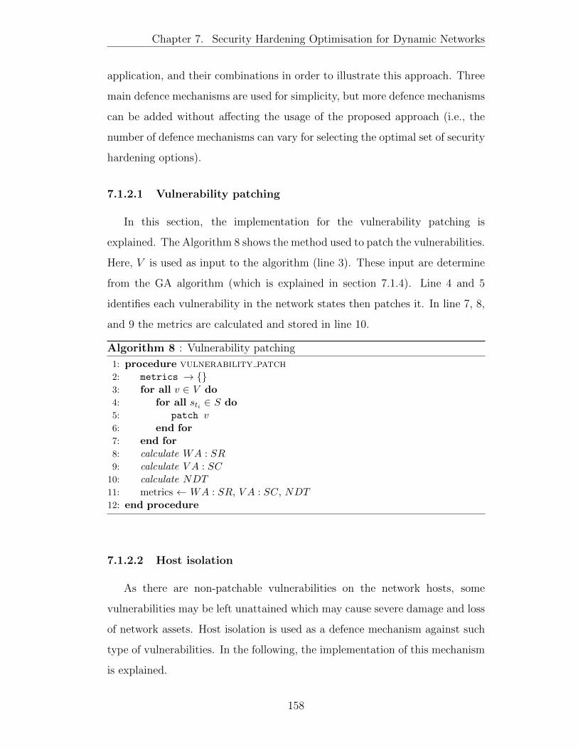
Chapter 7. Security Hardening Optimisation for Dynamic Networks
application, and their combinations in order to illustrate this approach. Three
main defence mechanisms are used for simplicity, but more defence mechanisms
can be added without affecting the usage of the proposed approach (i.e., the
number of defence mechanisms can vary for selecting the optimal set of security
hardening options).
7.1.2.1 Vulnerability patching
In this section, the implementation for the vulnerability patching is
explained. The Algorithm 8 shows the method used to patch the vulnerabilities.
Here, V is used as input to the algorithm (line 3). These input are determine
from the GA algorithm (which is explained in section 7.1.4). Line 4 and 5
identifies each vulnerability in the network states then patches it. In line 7, 8,
and 9 the metrics are calculated and stored in line 10.
Algorithm 8 : Vulnerability patching
1: procedure vulnerability patch2: metrics → {}3: for all v ∈ V do4: for all sti ∈ S do5: patch v6: end for7: end for8: calculate WA : SR9: calculate V A : SC
10: calculate NDT11: metrics ← WA : SR, V A : SC, NDT12: end procedure
7.1.2.2 Host isolation
As there are non-patchable vulnerabilities on the network hosts, some
vulnerabilities may be left unattained which may cause severe damage and loss
of network assets. Host isolation is used as a defence mechanism against such
type of vulnerabilities. In the following, the implementation of this mechanism
is explained.
158
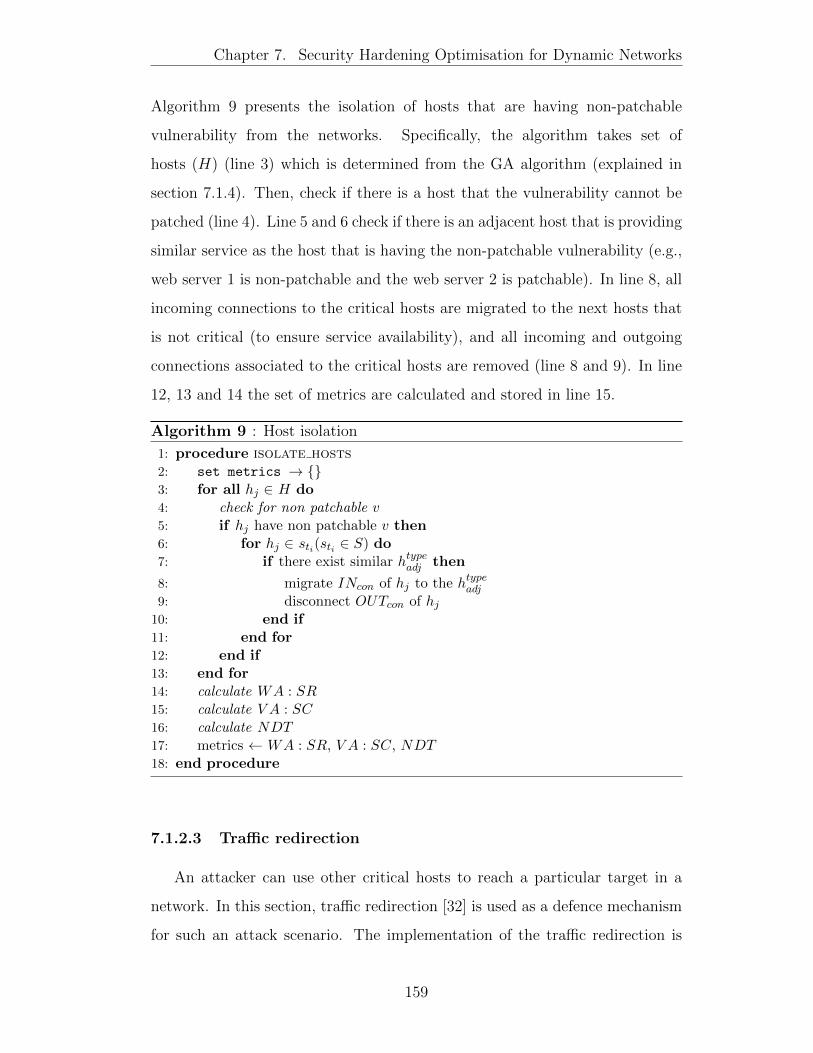
Chapter 7. Security Hardening Optimisation for Dynamic Networks
Algorithm 9 presents the isolation of hosts that are having non-patchable
vulnerability from the networks. Specifically, the algorithm takes set of
hosts (H) (line 3) which is determined from the GA algorithm (explained in
section 7.1.4). Then, check if there is a host that the vulnerability cannot be
patched (line 4). Line 5 and 6 check if there is an adjacent host that is providing
similar service as the host that is having the non-patchable vulnerability (e.g.,
web server 1 is non-patchable and the web server 2 is patchable). In line 8, all
incoming connections to the critical hosts are migrated to the next hosts that
is not critical (to ensure service availability), and all incoming and outgoing
connections associated to the critical hosts are removed (line 8 and 9). In line
12, 13 and 14 the set of metrics are calculated and stored in line 15.
Algorithm 9 : Host isolation
1: procedure isolate hosts2: set metrics → {}3: for all hj ∈ H do4: check for non patchable v5: if hj have non patchable v then6: for hj ∈ sti(sti ∈ S) do7: if there exist similar htypeadj then
8: migrate INcon of hj to the htypeadj
9: disconnect OUTcon of hj10: end if11: end for12: end if13: end for14: calculate WA : SR15: calculate V A : SC16: calculate NDT17: metrics ← WA : SR, V A : SC, NDT18: end procedure
7.1.2.3 Traffic redirection
An attacker can use other critical hosts to reach a particular target in a
network. In this section, traffic redirection [32] is used as a defence mechanism
for such an attack scenario. The implementation of the traffic redirection is
159
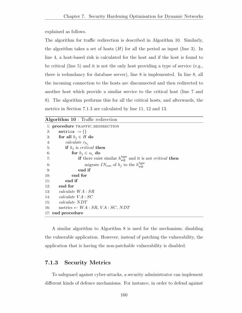
Chapter 7. Security Hardening Optimisation for Dynamic Networks
explained as follows.
The algorithm for traffic redirection is described in Algorithm 10. Similarly,
the algorithm takes a set of hosts (H) for all the period as input (line 3). In
line 4, a host-based risk is calculated for the host and if the host is found to
be critical (line 5) and it is not the only host providing a type of service (e.g.,
there is redundancy for database server), line 8 is implemented. In line 8, all
the incoming connection to the hosts are disconnected and then redirected to
another host which provide a similar service to the critical host (line 7 and
8). The algorithm performs this for all the critical hosts, and afterwards, the
metrics in Section 7.1.3 are calculated by line 11, 12 and 13.
Algorithm 10 : Traffic redirection
1: procedure traffic redirection2: metrics → {}3: for all hj ∈ H do4: calculate rhj5: if hj is critical then6: for hj ∈ sti do7: if there exist similar htypeadj and it is not critical then
8: migrate INcon of hj to the htypeadj
9: end if10: end for11: end if12: end for13: calculate WA : SR14: calculate V A : SC15: calculate NDT16: metrics ← WA : SR, V A : SC, NDT17: end procedure
A similar algorithm to Algorithm 8 is used for the mechanism; disabling
the vulnerable application. However, instead of patching the vulnerability, the
application that is having the non-patchable vulnerability is disabled.
7.1.3 Security Metrics
To safeguard against cyber-attacks, a security administrator can implement
different kinds of defence mechanisms. For instance, in order to defend against
160
Chapter 7. Security Hardening Optimisation for Dynamic Networks
the attacker exploiting a non-patchable vulnerability, the security administrator
may choose to isolate the hosts involved, disable the vulnerable application,
redirect traffics that are associated with the hosts, etc. For each of these
choices, the level of coverage, downtime and costs may be different. Moreover,
one or more of the options may be able to defend against multiple attack
scenarios. So, the security administrator is typically faced with the challenges
of evaluating and selecting the best options when there are multiple options
to select from. Security metrics [79] can be used to evaluate the effectiveness
of different security hardening options. However, they lack the capabilities to
understand the overall security posture of dynamic networks. In this section,
security metrics that take into account changes in network states (i.e., stateless
security risk, security cost and downtime of implementations) are used to
evaluate the effectiveness of the security hardening options for the dynamic
networks. The security metrics are described in Chapter 6.
7.1.4 Problem Formulation
In order to improve the security of networks, a set of security hardening
options can be selected from a pool of security solutions to be deployed.
However, computing the optimal security hardening set can be time-consuming,
and it becomes infeasible for large-sized networks as the solution search space
suffers from a state space explosion. Existing studies show that the solution
search space grows exponentially for an enumerated search [137] because there
are always 2n number of available choices, where there are a total of ‘n’ number
of options. With this number of choices, the enumerated search is not efficient
in finding the optimal solution [40].
Since the enumerated search is not suitable for finding the optimal
solution, the GA with three security objectives is considered. These security
objectives are: reducing the overall system risk, reducing the security hardening
implementation downtime and reducing the security cost of a dynamic network
given a fixed budget as a constraint. For the example dynamic networks, several
161
Chapter 7. Security Hardening Optimisation for Dynamic Networks
security hardening options are possible based on the vulnerability patching,
traffic redirection, disabling of applications and host isolations. The options
listed in Table 7.5 (which is computed from the T-HARM) are used as the
possible hardening options for the network. Applying any of these hardening
options may reduce the system risk, but at the same time will incur some
defence cost and may increase the downtime experienced as well. The focus of
this chapter is to find the optimal solutions that maximise the security while
minimising the defence cost and downtime given a fixed security budget as the
constraint. This will be achieved by optimally selecting the set of available
security hardening options under considerations. In the following, the security
hardening options are explained, and the optimisation problem is defined.
� Let P ∗ denote the set of vulnerabilities for the patch.
� Let Q∗ denote the set of hosts for possible isolation.
� Let D∗ be the set of traffics to drop.
� Let O∗ be the set of applications to disable.
� X∗ = P ∗ ∪Q∗ ∪D∗ ∪O∗ (i.e., is the set of all the hardening options).
Then the function f : X∗ → {0, 1} is used to describe the binary value
corresponding to each security hardening solution xi ∈ X∗ in the network. The
binary value indicates that a hardening option is deployed (1) or not deployed
(0). The security hardening vector (hv) for X∗ is defined as:
� hvX∗ = (f(x1), f(x2), ..., f(x|X∗|))
Then, the optimisation problem is formulated as shown in Definition 14.
Definition 14. The Optimisation Problem: Given a T-HARM and hvX∗ , find
the vector hvX∗ that optimises the objective functions:
Minimise (WA : SR(GSM, hvX∗), V A : SC(GSM, hvX∗), (NDT (GSM, hvX∗))
subject to: V A : SC ≤ SB,NDT ≤ DTC
162

Chapter 7. Security Hardening Optimisation for Dynamic Networks
where WA : SR(GSM, hvX∗), V A : SC(GSM, hvX∗) and NDT (GSM, hvX∗)
are the set of values from the objective functions of stateless risk (i.e., weighted
approach), security cost and downtime of implementations, respectively. SB
and DTC are the constraints imposed on security costs (i.e., a given security
budget) and the downtime of implementations, respectively.
Normally, there is no single global solution for a multi-objective problem
due to the conflicting nature of objective functions. As a result, the best trade-
off solutions called Pareto optimal solutions [110] are used for decision making.
The concept of the Pareto optimal solutions (Pareto frontier) is used to find
the set of optimal solutions for the defence options to deploy. In the following,
the Pareto optimal solutions for the optimisation problem is defined (which is
similar to the approach used in [110]). The constraints given in definition 14
determine the solution feasible region (FR).
Definition 15. Pareto optimal solutions: A solution, (WA : SR(GSM, hvX∗),
V A : SC(GSM, hvX∗), (NDT (GSM, hvX∗)) ∈ FR, is Pareto optimal iff
there does not exist another solution, (WA : SRβ(GSM, hvX∗β), V A :
SCβ(GSM, hvX∗β), NDTβ(GSM, hvX∗β)), such that
� WA : SRβ(GSM, hvX∗β) ≤ WA : SR(GSM, hvX∗) and V A :
SCβ(GSM, hvX∗β) ≤ V A : SC(GSM, hvX∗) and NDTβ(GSM, hvX∗β) ≤
NDT (GSM, hvX∗).
� WA : SRβ(GSM, hvX∗β) < WA : SR(GSM, hvX∗) or V A :
SCβ(GSM, hvX∗β) < V A : SC(GSM, hvX∗) or NDTβ(GSM, hvX∗β) <
NDT (GSM, hvX∗).
7.1.5 The Optimisation Approach
The optimisation steps are discussed in this section. The NSGA-II [110]
is used as the optimisation algorithm and the set of hardening options as the
input to the optimisation algorithm. The size of the hardening options is based
163
Chapter 7. Security Hardening Optimisation for Dynamic Networks
on the hardening options available. The T-HARM is used to determine all the
potential hardening options which can be deployed. The NSGA-II starts by
generating the initial population from the set of hardening options, where the
hardening options are encoded as binary values (i.e., chromosome), in which
1 indicates that a hardening option is deployed and 0 indicates that it is not
deployed. A generator is used to generate a possible deployment strategy (i.e., a
generation) using the concept of selection, crossover and mutation in the gene
(for child population or next generation) [39]. Each generation is evaluated
using the metrics outlined in Section 7.1.3 using the T-HARM, which the
results are passed to the optimisation algorithm. The optimisation algorithm
computes the optimal set of security hardening options to deploy based on the
fitness of the generations. A generation is a one-time iteration of the algorithm
(in the NSGA-II, a generation index is used to keep track of the number of
iterations). Therefore, the security administrator can define the maximum
number of generations that is required before the termination.
7.2 Simulations and Results
In this section, simulations are performed using two network models; (i)
small-scale network and (ii) large-scale network with up to 300 hosts, in order
to demonstrate the proposed approach. First, the sensitivity of the NSGA-II
to the input parameters are investigated. Then, the effect of different network
properties (e.g., multiple network states and varying network density) on the
optimum solutions is investigated (in particular, the varying of the number
of network states is considered). In Section 7.2.1, the simulation network, the
input for the metrics and the parameters used in the optimisation algorithm are
described. The result for the sensitivity analysis is presented in Section 7.2.2,
and the results for the effect of varying the number of states on the optimum
solutions shown in Section 7.2.4.
164
Chapter 7. Security Hardening Optimisation for Dynamic Networks
7.2.1 Simulation Network
An enterprise network which is divided into two subnets; DMZ and internal
network is used. The network topology is shown in Figure 7.1. The network
consists of five hosts and firewalls which protect access to the hosts in the
DMZ and internal network subnets. The OSes and applications in Table 7.2
are assumed to be running on the network hosts. Known patchable and non-
patchable vulnerabilities are collected from the NVD and [60] with respect
to the applications and operating system for each host in the network. The
vulnerabilities are shown in Table 7.1 and their distribution across the network
states in Table 7.2. Some of the vulnerabilities are patchable while other
are non-patchable. The non-patchable vulnerabilities are the vulnerabilities
that are without a patch at the time of this research. For example, the
vulnerability CVE-2012-1675 is an Oracle database 11g vulnerability that is
not fixed by a security patch update for this version of the database but a
configuration workaround is suggested to prevent attacker from exploiting this
vulnerability [1] (a detailed statistics of the non-patchable vulnerabilities and
faulty security patches can be found in [12]). Table 7.1 shows the vulnerabilities
of each host. Also, the non-patchable vulnerabilities are marked with the
symbol (*). However, it is worth noting that the security patches for these
vulnerabilities may be available at a later date as vendors usually take time
to provide some security patches for their products [12]. In Table 7.5, the
hardening options that apply to each of the states are shown. The attacker
model described in Section 3.2.2 is used.
Security metrics and economic values: In order to evaluate the
different attack scenarios and defence mechanisms, values for vulnerabilities
and the hardening options are used.
In specific, the impact metric for each vulnerability from the NVD is used
as aimv for the vulnerability and the prv is assigned based on the CVSS BS
version 2.0 [115].
165
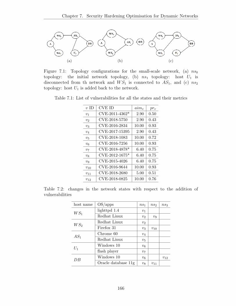
Chapter 7. Security Hardening Optimisation for Dynamic Networks
(a) (b) (c)
Figure 7.1: Topology configurations for the small-scale network, (a) ns0topology: the initial network topology, (b) ns1 topology: host U1 isdisconnected from th network and WS1 is connected to AS1, and (c) ns2topology: host U1 is added back to the network.
Table 7.1: List of vulnerabilities for all the states and their metrics
v ID CVE ID aimv prv
v1 CVE-2011-4362* 2.90 0.50
v2 CVE-2018-5750 2.90 0.43
v3 CVE-2016-2834 10.00 0.93
v4 CVE-2017-15395 2.90 0.43
v5 CVE-2018-1083 10.00 0.72
v6 CVE-2016-7256 10.00 0.93
v7 CVE-2018-4878* 6.40 0.75
v8 CVE-2012-1675* 6.40 0.75
v9 CVE-2015-4026 6.40 0.75
v10 CVE-2016-9644 10.00 0.93
v11 CVE-2018-2680 5.00 0.51
v12 CVE-2018-0825 10.00 0.76
Table 7.2: changes in the network states with respect to the addition ofvulnerabilities
host name OS/apps ns1 ns2 ns3
WS1lighttpd 1.4 v1Redhat Linux v2 v9
WS2Redhat Linux v2Firefox 31 v3 v10
AS1Chrome 60 v4Redhat Linux v5
U1Windows 10 v6flash player v7
DBWindows 10 v6 v12Oracle database 11g v8 v11
166
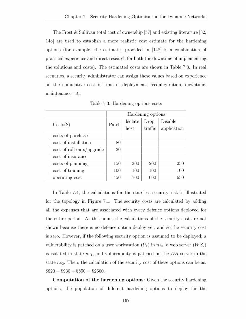
Chapter 7. Security Hardening Optimisation for Dynamic Networks
The Frost & Sullivan total cost of ownership [57] and existing literature [32,
148] are used to establish a more realistic cost estimate for the hardening
options (for example, the estimates provided in [148] is a combination of
practical experience and direct research for both the downtime of implementing
the solutions and costs). The estimated costs are shown in Table 7.3. In real
scenarios, a security administrator can assign these values based on experience
on the cumulative cost of time of deployment, reconfiguration, downtime,
maintenance, etc.
Table 7.3: Hardening options costs
Hardening options
Costs($) PatchIsolate
host
Drop
traffic
Disable
application
costs of purchase
cost of installation 80
cost of roll-outs/upgrade 20
cost of insurance
costs of planning 150 300 200 250
cost of training 100 100 100 100
operating cost 450 700 600 650
In Table 7.4, the calculations for the stateless security risk is illustrated
for the topology in Figure 7.1. The security costs are calculated by adding
all the expenses that are associated with every defence options deployed for
the entire period. At this point, the calculations of the security cost are not
shown because there is no defence option deploy yet, and so the security cost
is zero. However, if the following security option is assumed to be deployed; a
vulnerability is patched on a user workstation (U1) in ns0, a web server (WS2)
is isolated in state ns1, and vulnerability is patched on the DB server in the
state ns2. Then, the calculation of the security cost of these options can be as:
$820 + $930 + $850 = $2600.
Computation of the hardening options: Given the security hardening
options, the population of different hardening options to deploy for the
167
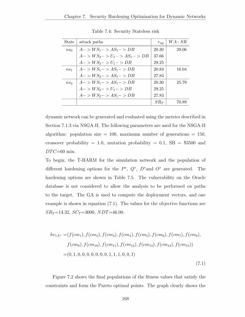
Chapter 7. Security Hardening Optimisation for Dynamic Networks
Table 7.4: Security Stateless risk
State attack paths rap WA : SR
ns0 A− > WS1− > AS1− > DB 20.30 29.06
A− > WS2− > U1− > AS1− > DB 37.66
A− > WS2− > U1− > DB 29.25
ns1 A− > WS1− > AS1− > DB 20.83 16.04
A− > WS2− > AS1− > DB 27.83
ns2 A− > WS1− > AS1− > DB 20.30 25.79
A− > WS2− > U1− > DB 29.25
A− > WS2− > AS1− > DB 27.83
SRT 70.89
dynamic network can be generated and evaluated using the metrics described in
Section 7.1.3 via NSGA-II. The following parameters are used for the NSGA-II
algorithm: population size = 100, maximum number of generations = 150,
crossover probability = 1.0, mutation probability = 0.1, SB = $3500 and
DTC=60 min.
To begin, the T-HARM for the simulation network and the population of
different hardening options for the P ∗, Q∗, D∗and O∗ are generated. The
hardening options are shown in Table 7.5. The vulnerability on the Oracle
database is not considered to allow the analysis to be performed on paths
to the target. The GA is used to compute the deployment vectors, and one
example is shown in equation (7.1). The values for the objective functions are
SRT=14.32, SCT=3000, NDT=46.00.
hv1X∗ =(f(cm1), f(cm2), f(cm3), f(cm4), f(cm5), f(cm6), f(cm7), f(cm8),
f(cm9), f(cm10), f(cm11), f(cm12), f(cm13), f(cm14), f(cm15))
=(0, 1, 0, 0, 0, 0, 0, 0, 0, 1, 1, 1, 0, 0, 1)
(7.1)
Figure 7.2 shows the final populations of the fitness values that satisfy the
constraints and form the Pareto optimal points. The graph clearly shows the
168
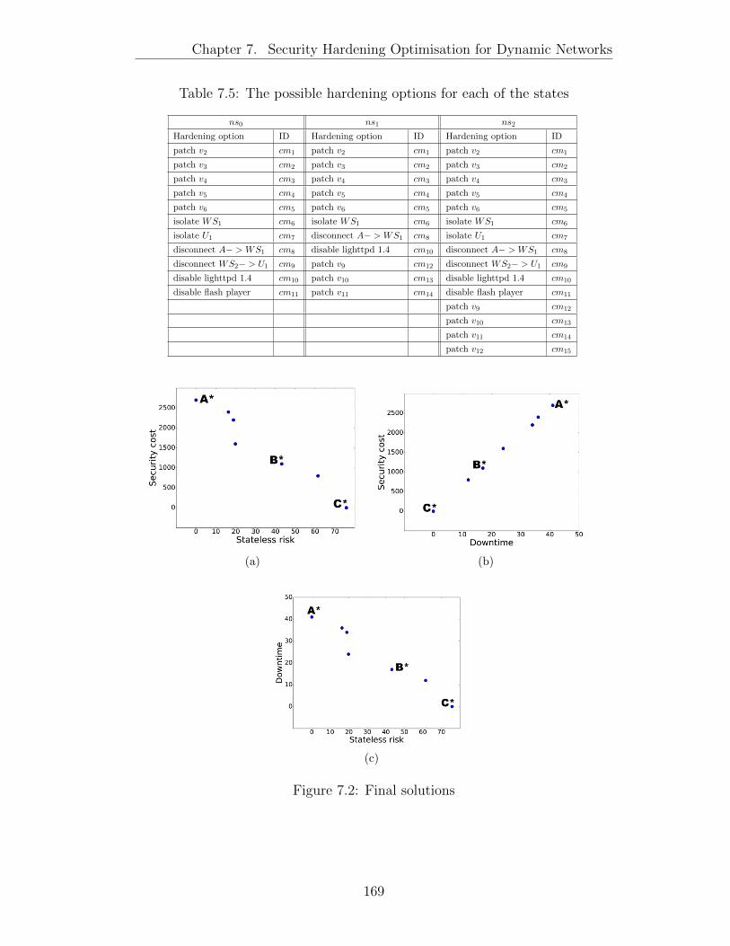
Chapter 7. Security Hardening Optimisation for Dynamic Networks
Table 7.5: The possible hardening options for each of the states
ns0 ns1 ns2
Hardening option ID Hardening option ID Hardening option ID
patch v2 cm1 patch v2 cm1 patch v2 cm1
patch v3 cm2 patch v3 cm2 patch v3 cm2
patch v4 cm3 patch v4 cm3 patch v4 cm3
patch v5 cm4 patch v5 cm4 patch v5 cm4
patch v6 cm5 patch v6 cm5 patch v6 cm5
isolate WS1 cm6 isolate WS1 cm6 isolate WS1 cm6
isolate U1 cm7 disconnect A− > WS1 cm8 isolate U1 cm7
disconnect A− > WS1 cm8 disable lighttpd 1.4 cm10 disconnect A− > WS1 cm8
disconnect WS2− > U1 cm9 patch v9 cm12 disconnect WS2− > U1 cm9
disable lighttpd 1.4 cm10 patch v10 cm13 disable lighttpd 1.4 cm10
disable flash player cm11 patch v11 cm14 disable flash player cm11
patch v9 cm12
patch v10 cm13
patch v11 cm14
patch v12 cm15
(a) (b)
(c)
Figure 7.2: Final solutions
169
Chapter 7. Security Hardening Optimisation for Dynamic Networks
trade-off between the three objective functions. For example, there are three
labelled points on the graphs (i.e., Figure 7.2(a), Figure 7.2(b) and Figure
7.2(c) ), where point A∗ shows the maximum SC (in Figure 7.2(a) and Figure
7.2(b)) and the maximum NDT (in Figure 7.2(b) and Figure 7.2(c) but have
the lowest at SR (in Figure 7.2(a) and Figure 7.2(c). The results show that
SC (security cost) and NDT (downtime of implementation) increases when
SR (risk) decrease. Here, one of the set of solutions is {patch v10, patch v4,
isolate U1, disconnect WS2− > U1, disable adobe flash player}.
The B∗ shows the intermediate solution among the final solutions (in terms
of fitness values). The solutions here is to {isolate WS1, disable lighttpd 1.4}.
While the point C∗ shows the other extreme point where the SC and NDT
are very low but the overall SR is high. Here, there is ‘null’ candidate to
implement.
7.2.2 Sensitivity Analysis
The simulation network is used to investigate the sensitivity of the NGSA-II
parameters. The algorithm parameters are set as described above. However,
in order to investigate the sensitivity of a particular parameter, only that
parameter is varied for the time. For example, in order to investigate
the sensitivity of the crossover probability, the population size, the number
of generations, mutations and budget are not varied while the crossover
probability is varied. The solutions obtained for each of the parameters are
compared against the real optimal solutions (i.e., the set of solutions that do
not change when parameters change). To begin, the crossover probability of
0.3, 0.5, 0.7 and 0.9 is used at different times. The results show that changing
the crossover probability only shows a negligible change in the set of solutions
obtained for them. However, Jun-chun et al. [90] have explained that the
crossover probability is more suitable for the large-scale network. So, the
various crossover probabilities may be more sensitive when a larger network
is considered. On the other hand, increasing the mutation probability shows
170

Chapter 7. Security Hardening Optimisation for Dynamic Networks
significant change for mutation probability 0.5, 0.7 and 0.9 with low accuracy
percentage compared to the real solutions (An example solution obtained for
these values are shown in Figure 7.3(b), Figure 7.3(c) and Figure 7.3(d),
respectively). For this case, some points are marked within the rectangle shape
to show a few points that match with the real optimum solutions. However,
it is worth noting that the set of solutions obtained for 0.5, 0.7 and 0.9 (i.e.,
high mutation probability) keep changing each time the algorithm is run and
so, may change when the algorithm is run again. Conversely, in Figure 7.3(a)
there is no change observed for the mutation probability values of 0.3 as the
results for the problem are always converging to optimal.
Similarly, the population size of 50, 100, 150, 200, 250 and 300 is used
respectively. The final solutions obtained remain the same for all the population
size (with a negligible difference in the accuracy of the solution for the
population size of 50). Furthermore, the same results are obtained for the
case of increasing the number of generations from 50 to 300.
7.2.3 Processing Time
Further analysis is performed to investigate the processing time of the GA
when the following parameters are increased; (1) the population size and (2) the
maximum number of generations. The accuracy of the results for the (1) and
(2) compared to a best-case solution are then presented. Here, the accuracy
is defined as the percentage of the number of Pareto optimum points for each
parameter that is varied compared to the best case solutions. The best case
solutions are the set of Pareto optimum points that do not change when the
population size or the number of generations is increased further.
The network model in Section 7.1.1 is used to construct a generic network
that randomly connects hosts in each state (with each host connected to at
least three other hosts). Three network states with each state having 100 hosts
are captured (i.e., 300 hosts are analysed for the entire time window). Similarly,
the attacker model in Section 3.2.2 is used to construct the corresponding T-
171
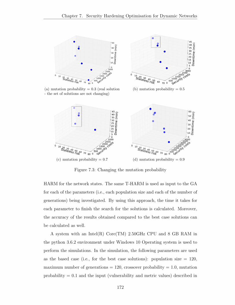
Chapter 7. Security Hardening Optimisation for Dynamic Networks
Stateless risk
0 10 20 30 40 50 60 70 80 Securit
y costs
0500
10001500
20002500
3000
Dow
nti
me (
min
)
0
10
20
30
40
50
(a) mutation probability = 0.3 (real solution- the set of solutions are not changing)
(b) mutation probability = 0.5
(c) mutation probability = 0.7
Stateless risk
0 10 20 30 40 50 60 70 80 Securit
y costs
0500
10001500
20002500
30003500
4000
Dow
nti
me (
min
)
0
10
20
30
40
50
60
(d) mutation probability = 0.9
Figure 7.3: Changing the mutation probability
HARM for the network states. The same T-HARM is used as input to the GA
for each of the parameters (i.e., each population size and each of the number of
generations) being investigated. By using this approach, the time it takes for
each parameter to finish the search for the solutions is calculated. Moreover,
the accuracy of the results obtained compared to the best case solutions can
be calculated as well.
A system with an Intel(R) Core(TM) 2.50GHz CPU and 8 GB RAM in
the python 3.6.2 environment under Windows 10 Operating system is used to
perform the simulations. In the simulation, the following parameters are used
as the based case (i.e., for the best case solutions): population size = 120,
maximum number of generations = 120, crossover probability = 1.0, mutation
probability = 0.1 and the input (vulnerability and metric values) described in
172
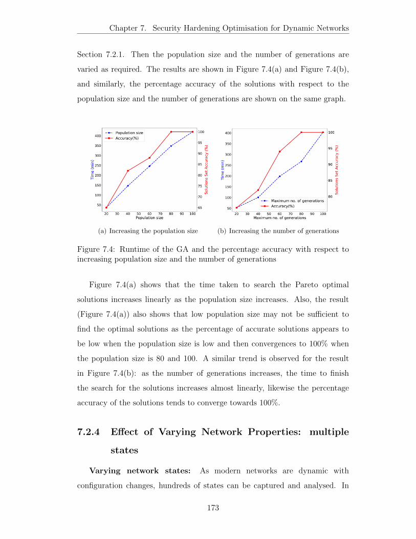
Chapter 7. Security Hardening Optimisation for Dynamic Networks
Section 7.2.1. Then the population size and the number of generations are
varied as required. The results are shown in Figure 7.4(a) and Figure 7.4(b),
and similarly, the percentage accuracy of the solutions with respect to the
population size and the number of generations are shown on the same graph.
(a) Increasing the population size (b) Increasing the number of generations
Figure 7.4: Runtime of the GA and the percentage accuracy with respect toincreasing population size and the number of generations
Figure 7.4(a) shows that the time taken to search the Pareto optimal
solutions increases linearly as the population size increases. Also, the result
(Figure 7.4(a)) also shows that low population size may not be sufficient to
find the optimal solutions as the percentage of accurate solutions appears to
be low when the population size is low and then convergences to 100% when
the population size is 80 and 100. A similar trend is observed for the result
in Figure 7.4(b): as the number of generations increases, the time to finish
the search for the solutions increases almost linearly, likewise the percentage
accuracy of the solutions tends to converge towards 100%.
7.2.4 Effect of Varying Network Properties: multiple
states
Varying network states: As modern networks are dynamic with
configuration changes, hundreds of states can be captured and analysed. In
173

Chapter 7. Security Hardening Optimisation for Dynamic Networks
this section, the effect of varying the number of states on the optimal solutions
and the network security posture is investigated. Specifically, the number of
network states is varied incrementally, and then how the optimal solutions
are affected are observed. A network which is similar to Figure 7.2.1 is used
but with randomly generated dynamic network properties (e.g., addition of
hosts, removal of hosts, removal of edges, etc). Several states are captured
for this simulation (as required). Based on the sensitivity analysis performed
in section 7.2.2, the parameter are used as: population size = 120, maximum
number of generations = 150, crossover probability = 1.0, mutation probability
= 0.1, SB = $3500 and DTC=60 min in the optimisation algorithm. In
Figure 7.5, the results for the different number of states are shown.
The results in Figure 7.5 show that varying the number of network states
affect the optimal set of solutions. Also, it is observed that a few of the Pareto
optimal points for a pair of consecutive states show similar points. However,
manual inspection of the set of solutions for deployment for those points showed
that the set of solutions varied among the states. Therefore, a conclusion can
be made that the optimal set of solutions changes as the network configuration
changes over time for dynamic networks.
174
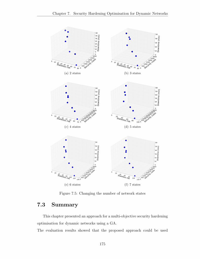
Chapter 7. Security Hardening Optimisation for Dynamic Networks
Stateless risk
0 10 20 30 40 50 6070
80 Securit
y co
sts
0500
10001500
20002500
3000
Dow
nti
me (
min
)
0
5
10
15
20
25
30
35
40
(a) 2 states
Stateless risk
0 10 20 30 40 50 60 70 80 Securit
y cos
ts
0500
10001500
20002500
3000
Dow
nti
me (
min
)
0
10
20
30
40
50
(b) 3 states
Stateless risk
010
2030
4050
6070 Secu
rity c
osts
0500
10001500
20002500
30003500
4000
Dow
nti
me (
min
)
0
10
20
30
40
50
60
(c) 4 states
Stateless risk
020
4060
80100 Secu
rity c
osts
0500
10001500
20002500
30003500
4000
Dow
nti
me (
min
)
0
10
20
30
40
50
60
(d) 5 states
Stateless risk
020
4060
80100
120140
Secu
rity
cost
s
0500
10001500
20002500
30003500
4000
Dow
nti
me (
min
)
0
10
20
30
40
50
60
(e) 6 states
Stateless risk
020
4060
80100
120Sec
urity
cost
s
0500
10001500
20002500
30003500
4000
Dow
nti
me (
min
)
0
10
20
30
40
50
60
(f) 7 states
Figure 7.5: Changing the number of network states
7.3 Summary
This chapter presented an approach for a multi-objective security hardening
optimisation for dynamic networks using a GA.
The evaluation results showed that the proposed approach could be used
175
Chapter 7. Security Hardening Optimisation for Dynamic Networks
to aid security administrators in selecting and deploying an optimal set of
security hardening options for dynamic networks. The results also showed
that multiple optimal sets satisfy the multi-objectives while satisfying the
constraints. Further, it showed that the optimal set changes as the network
configuration change over time for dynamic networks. Therefore, the proposed
approach can support security administrators with an overview of how the
optimal solution changes over time, as well as compute the optimal solution
taking into account changes made by dynamic networks. Moreover, the security
administrator can understand the pros and cons of each option before deploying
them.
176
Chapter 8
Discussions and Future Work
Changes in dynamic networks affect the security posture of the network.
Thus, understanding the security posture of dynamic networks is difficult,
especially when a new set of attack vectors are introduced as a result of
the changes. Traditional GSMs and metrics, such as AGs and probability
of attack success, are used to evaluate the security posture of the network.
However, these approaches assumed the network of static nature. As such,
changes that happen as a result of hosts joining, host disconnecting, new
vulnerabilities discovered, etc. which changes the security posture are not
captured using the traditional GSMs and the existing security metrics. Hence,
security analysis based on them are not comprehensive to capture the changes
that are happening in the networks. This is important in order to provide an
efficient defence approach for the security of dynamic networks.
The research presented in this thesis is intended to provide the computer
networking and security communities with methods to assess and harden the
security of modern networks that are dynamic with configurations changes
(e.g., SDN and Cloud networks). T-HARM and TI-HARM are developed to
assess the security of networks, and also show different aspects of the security
of the dynamic networks (specifically, the T-HARM provides the temporal
security states of dynamic networks while the TI-HARM provide the time-
independent view of a dynamic network). Besides, metrics to assess the
177
Chapter 8. Discussions and Future Work
security of dynamic networks are developed to show the security changes in
the network quantitatively. Lastly, an approach to optimally select security
hardening solutions for dynamic networks from a pool of options (under
multiple constraints) was proposed. However, several assumptions are made
in this thesis which requires further research in order to enhance the proposed
approaches. This chapter discusses the limitations of the approaches and points
out further research directions.
8.1 Addressing the Research Questions
As outline in Chapter 1, this thesis uses security modelling approach to
answer the following questions:
� Q1: what are the approaches that be used to systematically capture and
model the attack scenarios in dynamic networks?
� Q2: what are the characteristics of dynamic networks, and how can we
quantitatively measure the security of the dynamic networks?
� Q3: what approach can be used to select the optimal security hardening
solutions for dynamic networks taking into account multiple objectives
(e.g., maximise security and minimise cost)?
To address the research question Q1, a temporal GSM (named T-HARM)
and a time-independent GSM (named TI-HARM) are developed in Chapter 3
and Chapter 5, respectively. In particular, the T-HARM captures and analyse
the potential attack scenarios of the temporal networks at every time t (i.e., on
multiple GSM). While the TI-HARM captures and aggregates all the observed
attack scenarios onto one GSM. The formalism and security assessment for the
proposed GSMs are given and demonstrated with examples and experimental
analysis via simulations. Moreover, a systematic classification of network
changes and their formalisms with respect to security changes are also given in
Chapter 3.
178
Chapter 8. Discussions and Future Work
To address the research question Q2, a comprehensive evaluation of the
existing security metrics is performed in Chapter 4, in order to identify which
one is suitable or not suitable for the analysis of dynamic networks. Also, the
functionality of the T-HARM and TI-HARM are utilised to develop a new
set of metrics (in Chapter 6) to quantitatively assess the security of dynamic
networks. The usability of the proposed metrics is shown through simulations
and examples.
To address the research question Q3, a security optimisation approach with
heterogeneous hardening options (i.e., hosts isolation, vulnerability patching,
traffic redirection, etc) for dynamic networks is developed (in Chapter 7). The
optimal deployment solution is computed via the T-HARM while taking into
account the limited security budget and time of implementations as constraints.
The feasibility of the proposed approach is demonstrated for a real-world
scenario by considering the existence of both patchable and non-patchable
vulnerabilities.
The proposed approaches can be applied to dynamic enterprise networks
and emerging networking technologies, such as SDN [98] and cloud
computing [113]. Moreover, the T-HARM can be used to model and assess
the effectiveness of dynamic security solutions (e.g., MTD with the dynamic
metrics) [71].
Besides, the proposed optimisation approach can be employed for decision
making in the presence of many sets of possible hardening solution to deploy
when there are constraints such as costs to keep up with.
8.2 Limitations and Future Work
This thesis has some limitations that need to be addressed in the future
work in order to extend the research scope. In the following, the limitations
and the future work are explained.
179
Chapter 8. Discussions and Future Work
8.2.1 Different network characteristics
Although a typical enterprise network configurations are considered for the
experiments but generally, a network can be complex with different types of
network topologies or a combination of different topologies (e.g., a combination
of star and ring) [10, 161]. This thesis did not consider different types of
network topologies and network density and how the various characteristics
affect security metrics in a dynamic network. Thus, it is important to consider
how the different topologies and network density can affect the security of
dynamic networks. Moreover, the flexibility and diversity experienced in a
heterogeneous network environment [107] changes the security posture of the
network continuously, and hence this makes the network more vulnerable to
several types of cyber-attack which were not covered in this thesis.
Furthermore, this thesis did not consider other network technologies such
as Cloud and IoT [62] in the categorisation of the network changes. Hence,
there is a need to perform a more detailed categorisation of modern network
changes (for Cloud, IoT, etc.) with their respective correlation to the changes
in GSMs in order to perform more analysis.
8.2.2 Dynamic Models
A temporal GSM named T-HARM was developed. The T-HARM takes
snapshots of the dynamic network at every time point and then dynamically
analysed the security. Despite this, modern networks (e.g., Cloud and SDN)
usually allow their components to change even more frequently (than enterprise
networks) [84] and in consequence, a critical network state (for effective security
analysis) can be skipped. Therefore, there is a need of an on-line T-HARM
which tracks network changes in real time and then automatically adjust
to changes in the security posture of the network. This approach can be
done periodically or when a certain percentage of changes are detected in the
network.
180
Chapter 8. Discussions and Future Work
8.2.3 Attacker Models
In the attacker model, a single target host and a single attacker is
considered. Also, an internal attacker who wants to compromise hosts in the
internal network is not considered as well. However, multiple attackers trying
to compromise different targets can be modelled [134]. So, more research is
needed to consider attacker models with multiple attackers, internal attackers
and multiple targets, as well as considering various attack scenarios (e.g.,
Distributed Denial of Service attack [116]).
Besides, our attacker model assumes the same level of behaviour and
capability for the attacker. However, real-world attackers can have different
behaviours and capabilities which our GSM did not take into account. As a
result, this limits our proposed approach to model different kinds of attacks
along with the changes in the behaviour of the attacker. To extend our
proposed approach, a separate component (or module) which explicitly model
the changes in the attacker’s behaviour or the attacker’s capabilities can be
incorporated [83, 133]. Thus, this will allow the security administrator to
perform several types of security analysis (e.g., based on the behaviour or
capabilities of the attacker).
8.2.4 Security metrics
The varying effects of eleven (11) security metrics is investigated when
various changes are observed in the network. However, there are many
other quantitative security metrics for assessing the security of networks (e.g.,
weakest adversary metrics [129], network compromise percentage [104], attack
resistant metric [159], K-zero day safety [158], attack surface metric [109], etc).
So, more comprehensive evaluation of those security metrics for assessing the
security of dynamic networks is required. Besides, Bopche and Mehtre [19]
proposed graph distance metrics for dynamic security analysis. In particular,
they used maximum common sub-graph and graph edit distance metric to
181
Chapter 8. Discussions and Future Work
quantify the distance between a pair of successive AGs generated for a dynamic
network. However, these metrics are used with AGs, and it is still unknown
how they will change when they are used for dynamic GSMs.
8.2.5 Optimal Defence Models
� Defence mechanism: In this thesis, a heterogeneous hardening option
is considered as the proactive defence mechanism. This thesis showed that
these hardening options can be integrated into the T-HARM. However,
many proactive defence mechanisms were not considered. So, more
defence options should be integrated into the model in the future work.
It is believed that incorporating more defence mechanisms may further
provide better optimum solutions.
� Patchable and non-patchable vulnerabilities: In this work, the
feasibility of this approach for real-world network scenarios which are
having both patchable and non-patchable vulnerabilities is demonstrated.
However, unknown vulnerabilities are not considered. Therefore there is a
need to consider the unknown vulnerabilities in the future work. Besides,
the impact of the existence of the unknown vulnerabilities in the security
of the networks and selection of optimal hardening solutions needs to be
investigated.
� Dynamic security metrics: To the best of our knowledge, this is
the first work to use dynamic security metrics (as fitness functions)
to evaluate the effectiveness of security hardening options in the multi-
objective optimisation problem (for the security of dynamic networks).
Security stateless risk, downtime of implementation and security cost
are used, and then the trade-off solutions between them is computed.
However, to fully find the optimal solutions for real networks where best
users’ experiences are minimally affected, then there is a need to consider
both security, cost, performance and availability. In the future, the
182
Chapter 8. Discussions and Future Work
Symbolic Hierarchical Automated Reliability and Performance Evaluator
(SHARPE) [138] can be used to calculate the performance and availability
metrics which will be incorporated as additional fitness functions to the
optimisation algorithm.
� Optimisation algorithms: The results showed that the NSGA-II
provides a good spread of solutions over the Pareto optimal set for
the three objective functions that were considered. However, there are
computational complexity which this study did not take into account.
Therefore, in the future work, there is a need to find an approach to
reduce the time complexity that is caused by the paths calculations
in the evaluations of the fitness function (security stateless risk). The
calculation (attack path calculations) of the metric took so much time
which resulted in a long time to finish the search for optimal solutions
when the population size and number of generations is increased. Besides,
other optimisation algorithms need to be evaluated for the most efficient
algorithm to use compared to the GA in terms of speed.
8.2.6 Validation
Although practical data from a university network is collected, they were
not used in this thesis because of constraints (e.g., time and university
security policies). However, real-world network settings data (e.g., security
vulnerabilities by NVD [119]) are used to model changes in vulnerabilities in
the simulations. To overcome this limitation, a test-bed network can be set-up
and then various data can be collected (as required) to validate this approaches
in more simulations.
183

Chapter 9
Conclusions
Dynamic networks can be characterised by many factors such as changes
(e.g., vulnerability change, the update of applications and services, topology
changes). There is a lack of methods and techniques to capture different
security posture when the network changes. Consequently, it is difficult to
assess the security of the dynamic networks which changes over time. This
thesis identified three major problems with the existing security models, their
assessment methods and selection of security hardening options for dynamic
networks. First, the assumptions of existing security models that networks are
static in nature makes it insufficient to capture and analyse the security of
dynamic networks. Secondly, the security metrics have been designed from the
perspective of static networks, and so, it is difficult to estimate how existing
security metrics will change as the network changes over time, since current
metrics have only been used to assess the static networks. Thirdly, changes
in the configurations of network states affect the optimal hardening solutions;
therefore the optimal solutions calculated by the existing approach may not be
optimum for networks that change over time.
So, in this thesis, four distinct contributions to knowledge in the networks
security modelling, assessment and security hardening are made. They are
listed as follows.
184

Chapter 9. Conclusions
1. This thesis has presented two variant security models to capture and
analyse the security posture of dynamic networks. First, a GSM named
T-HARM that captures changes in dynamic networks every time t was
developed. Then, the T-HARM was formalised, and the approach
to assess the security of the dynamic network via the T-HARM was
shown. Secondly, a time-independent GSM (named TI-HARM) which
takes into account multiple network states, duration and the visibility
of components in the states was developed to comprehensively model
and analyse the security of changing networks onto a single GSM. The
use of different weight threshold for the TI-HARM was shown, and the
effect of using different weight threshold to construct the TI-HARM was
investigated. Besides, an algorithm for determining the MWT to use in
order to prevent misleading security analysis when using the TI-HARM
was developed as well.
2. A systematic evaluation of existing security metrics has been presented.
In the beginning, a categorisation of various network changes based on
the causes of the change was performed. Then, based on the changes
identified, a comprehensive evaluation of the existing security metrics
was performed. The results were summarised based to their effectiveness
to security changes. A security/network administrator can determine
the security metric that will effectively present the security posture of a
network when a specific type of network configuration change occurs.
3. New set of metrics to assess the security of dynamic networks have been
developed. Also, a categorisation of metrics based on their functionalities
and what they present has been presented. Examples and simulations are
used to demonstrate the usability and quantification of these metrics.
4. An approach for the security optimisation of dynamic network has
been developed. In particular, an approach for multi-objective security
hardening optimisation for dynamic networks using a GA was presented.
185
Chapter 9. Conclusions
The T-HARM was used, and the optimisation problem was implemented
using the NSGA-II algorithm with the input generated from the T-
HARM. Multiple objectives and constraints were taken into accounts,
such as security and cost, and the effectiveness of the optimal set of
security hardening options are computed. For the evaluations, a dynamic
network scenario with patchable and non-patchable vulnerabilities was
considered, with both vulnerability patching, traffic redirections and
host isolations as proactive defence mechanisms. The evaluation results
showed that the proposed approach could be used to aid security
administrators in selecting and deploying an optimal set of security
hardening options. The results also showed that multiple optimal sets
satisfy the multi-objectives while satisfying the constraints. The results
also showed that the optimal set changes as the network configuration
change over time for dynamic networks.
In general, the proposed dynamic models are capable of modelling the attack
scenarios from multiple network states. Together with the developed security
metrics, they can quantitatively assess the security of dynamic networks. The
proposed optimisation approach can support security administrators with an
overview of how the optimal solution changes over time, as well as compute the
optimal solution by taking into account changes made by dynamic networks
and other constraints. Moreover, this approach provides a way for the security
administrator to understand the pros and cons of each hardening option before
their deployment.
186
References
[1] Oracle Security Alert CVE-2012-1675, 2018 (accessed June 5, 2018).
https://support.symantec.com/en_US/article.TECH219444.html.
[2] M. S. Ahmed, E. Al-Shaer, and L. Khan. A Novel Quantitative Approach
For Measuring Network Security. In Proceedings of the 27th IEEE
Conference on Computer Communications (INFOCOM), pages 1957–
1965. IEEE, April 2008.
[3] M. Albanese, S. Jajodia, and S. Noel. Time-efficient and Cost-effective
Network Hardening Using Attack Graphs. In Proceedings of the 42nd
Annual IEEE/IFIP International Conference on Dependable Systems and
Networks (DSN), pages 1–12, Washington, DC, USA, June 2012. IEEE.
[4] J. Almasizadeh and M. A. Azgomi. A Stochastic Model of Attack Process
for the Evaluation of Security Metrics. Computer Networks, 57(10):2159–
2180.
[5] H. M. J. Almohri, L. T. Watson, D. Yao, and X. Ou. Security
Optimization of Dynamic Networks with Probabilistic Graph Modeling
and Linear Programming. IEEE Transactions on Dependable and Secure
Computing (TDSC), 13(4):474–487, July 2016.
[6] F. Arnold, D. Guck, R. Kumar, and M. Stoelinga. Sequential and Parallel
Attack Tree Modelling. In Proceedings of the International Conference on
Computer Safety, Reliability and Security (SAFECOMP), pages 291–299,
Cham, 2015. Springer International Publishing.
187

References
[7] A. Arora, C. Forman, A. Nandkumar, and R. Telang. Competitive and
Strategic Effects in the Timing of Patch Release. In Fifth Workshop
Economic Information Security (WEIS), June 2006.
[8] A. Avizienis, J. C. Laprie, B. Randell, and C. Landwehr. Basic Concepts
and Taxonomy of Dependable and Secure Computing. IEEE Transactions
on Dependable and Secure Computing (TDSC), 1(1):11–33, Jan 2004.
[9] D. Baca and K. Petersen. Prioritizing Countermeasures Through the
Countermeasure Method for Software Security (CM-Sec). In Proceedings
of the 11th International Conference on Product-Focused Software
Process Improvement (PROFES), pages 176–190, Berlin, Heidelberg,
2010. Springer-Verlag.
[10] A.-L. Barabasi, R. Albert, and H. Jeong. Scale-free Characteristics of
Random Networks: The Topology of the World-Wide Web. Physica A:
Statistical Mechanics and its Applications, 281(1-4):69–77, 2000.
[11] C. Barker. NIST Security Measurement NIST SP 800-55 Revision 1,
2007 (accessed February 20, 2016). http://csrc.nist.gov/groups/
SMA/ispab/documents/minutes/2007-09/Barker_ISPAB_
Sept2007-SP800-55R1.pdf.
[12] S. Beattie, S. Arnold, C. Cowan, P. Wagle, C. Wright, and A. Shostack.
Timing the Application of Security Patches for Optimal Uptime. In
Proceedings of the 16th USENIX Conference on System Administration
(LISA), pages 233–242, Berkeley, CA, USA, 2002. USENIX Association.
[13] S. Bistarelli, F. Fioravanti, and P. Peretti. Defense Trees for
Economic Evaluation of Security Investments. In Proceedings of the
First International Conference on Availability, Reliability and Security
(ARES), pages 416–423. IEEE, April 2006.
188
References
[14] S. Bistarelli, F. Fioravanti, P. Peretti, and F. Santini. Evaluation of
Complex Security Scenarios using Defense Trees and Economic Indexes.
Journal of Experimental & Theoretical Artificial Intelligence, 24(2):161–
192, 2012.
[15] R. Bohme. Security Metrics and Security Investment Models. In
I. Echizen, N. Kunihiro, and R. Sasaki, editors, International Workshop
on Security: Advances in Information and Computer Security (IWSEC),
pages 10–24, Berlin, Heidelberg, 2010. Springer Berlin Heidelberg.
[16] R. Bohme and T. Moore. Security Metrics and Security Investment. 2013.
At: https://tylermoore.ens.utulsa.edu/courses/econsec/reading/lnse-
secinv2.pdf.
[17] R. Bojanc and B. Jerman-Blazic. An Economic Modelling Approach
to Information Security Risk Management. International Journal of
Information Management, 28(5):413 – 422, 2008.
[18] H. Bootsma, O. Curet, A. de Leeuw, A. Leijenhorst, W. Mocking, and
D. Stewart. 2009 TMT Global Security Survey, Technical Report, (2009).
Deloitte Touche Tohmatsu.
[19] G. S. Bopche and B. M. Mehtre. Graph Similarity Metrics for Assessing
Temporal Changes in Attack Surface of Dynamic Networks. Computer
& Security, 64(C):16–43, Jan. 2017.
[20] D. Borbor, L. Wang, S. Jajodia, and A. Singhal. Securing Networks
Against Unpatchable and Unknown Vulnerabilities Using Heterogeneous
Hardening Options. In G. Livraga and S. Zhu, editors, Data and
Applications Security and Privacy XXXI, pages 509–528, Cham, 2017.
Springer International Publishing.
189

References
[21] D. Borbor, L. Wang, S. Jajodia, and A. Singhal. Surviving Unpatchable
Vulnerabilities through Heterogeneous Network Hardening Options.
Journal of Computer Security, Preprint(Preprint):1–29, July 2018.
[22] D. Braha and Y. Bar-Yam. From Centrality to Temporal Fame: Dynamic
Centrality in Complex Networks. In Social Science Research Network
Working Paper Series, 2006.
[23] R. Breu, F. Innerhofer-Oberperfler, and A. Yautsiukhin. Quantitative
Assessment of Enterprise Security System. In Third International
Conference on Availability, Reliability and Security (ARES), pages 921–
928, March 2008.
[24] B. Brykczynski and R. A. Small. Reducing Internet-Based Intrusions:
Effective Security Patch Management. IEEE Software, 20(1):50–57, Jan.
2003.
[25] B.-M. Bui-Xuan, A. Ferreira, and A. Jarry. Evolving Graphs and least
Cost Journeys in Dynamic Networks. In Modeling and Optimization
in Mobile, Ad Hoc and Wireless Networks (WIOPT), Sophia Antipolis,
France, Mar. 2003.
[26] A. Buldas and T. Magi. Practical Security Analysis of E-Voting Systems.
Springer Berlin Heidelberg, Berlin, Heidelberg, 2007.
[27] E. J. Byres, M. Franz, and D. Miller. The Use of Attack Trees in Assessing
Vulnerabilities in Scada Systems. In Proceedings of the International
Infrastructure Survivability Workshop (IISW), pages 3–10. IEEE, 2004.
[28] A. Casteigts, P. Flocchini, W. Quattrociocchi, and N. Santoro. Time-
Varying Graphs and Dynamic Networks. In Proceedings of 10th
International Conference on Ad-hoc, Mobile, and Wireless Networks
(ADHOC-NOW), pages 346–359, Berlin, Heidelberg, 2011. Springer
Berlin Heidelberg.
190

References
[29] U.-C. S. O. Center. NIST Information Technology Laboratory, National
Vulnerability Database, 2017 (accessed September 23, 2017). https:
//nvd.nist.gov/vuln-metrics/cvss.
[30] F. Chen, D. liu, Y. ZhanG, and J. Su. A Scalable Approach to Analyzing
Network Security using Compact Attack Graph. In Journal of Networks,
volume 5, page 543, 2010.
[31] Y. Cherdantseva, P. Burnap, A. Blyth, P. Eden, K. Jones, H. Soulsby,
and K. Stoddart. A Review of Cyber Security Risk Assessment Methods
for SCADA Systems. Computers and Security, 56(2):1 – 27, 2016.
[32] C. J. Chung, P. Khatkar, T. Xing, J. Lee, and D. Huang. NICE: Network
Intrusion Detection and Countermeasure Selection in Virtual Network
Systems. IEEE Transactions on Dependable and Secure Computing
(TDSC), 10(4):198–211, July 2013.
[33] CIS. The Center for Internet Security: Security Metrics, accessed April
21, 2017. https://benchmarks.cisecurity.org/tools2/metrics/
CIS_Security_Metrics_v1.1.0.pdf.
[34] M. Cremonini and P. Martini. Evaluating Information Security
Investments from Attackers Perspective: The Return-On-Attack (ROA).
In Fourth Workshop on the Economics of Information Security (WEIS),
June 2005.
[35] CVSS. CVSS Calculator, 2016 (accessed February 27, 2016). https:
//nvd.nist.gov/CVSS-v2-Calculator/CVSS-v2-Equations.
[36] CVSS. CVSS version 3 - Forum for Response and Security Team,
accessed March 20, 2017. https://www.first.org/cvss.
[37] B. Danev, R. Masti, G. Karame, and S. Capkun. Enabling Secure
VM-vTPM Migration in Private Clouds. In Proceedings of the Annual
191
References
Computer Security Applications Conference (ACSAC), pages 187–196.
ACM, 2011.
[38] S. Das, A. Mandal, and R. Mukherjee. An Adaptive Differential Evolution
Algorithm for Global Optimization in Dynamic Environments. IEEE
Transactions on Cybernetics, 44(6):966–978, June 2014.
[39] K. Deb, S. Agrawal, A. Pratap, and T. Meyarivan. A Fast Elitist Non-
dominated Sorting Genetic Algorithm for Multi-objective Optimization:
NSGA-II. In International Conference on Parallel Problem Solving From
Nature (PPSN), pages 849–858. Springer, 2000.
[40] R. Dewri, N. Poolsappasit, I. Ray, and D. Whitley. Optimal Security
Hardening Using Multi-objective Optimization on Attack Tree Models of
Networks. In Proceedings of the 14th ACM Conference on Computer and
Communications Security (CCS), pages 204–213, 2007.
[41] R. Dewri, I. Ray, N. Poolsappasit, and D. Whitley. Optimal Security
Hardening on Attack Tree Models of Networks: A Cost-benefit Analysis.
International Journal of Information Security, 11(3):167–188, June 2012.
[42] S. Donohue. Distribution of Software Updates via a Computer Network,
Mar. 6 2001. US Patent 6,199,204.
[43] K. Edge, R. Raines, M. Grimaila, R. Baldwin, R. Bennington, and
C. Reuter. The use of Attack and Protection Trees to Analyze Security
for an Online Banking System. In 40th Annual Hawaii International
Conference on System Sciences (HICSS). IEEE, 2007.
[44] K. A. Edge. A Framework for Analyzing and Mitigating the
Vulnerabilities of Complex Systems via Attack and Protection Trees.
Ph.D. Thesis - Air Force Institute of Technology, 2007.
[45] K. S. Edge, G. C. Dalton, R. A. Raines, and R. F. Mills. Using Attack and
Protection Trees to Analyze Threats and Defenses to Homeland Security.
192

References
In Proceedings of the 2006 IEEE Conference on Military Communications
(MILCOM), pages 953–959, Piscataway, NJ, USA, 2006.
[46] S. Y. Enoch, M. Ge, J. B. Hong, H. Alzaid, and D. S. Kim. Evaluating the
Effectiveness of Security Metrics for Dynamic Networks. In Proceedings of
the 16th IEEE International Conference on Trust, Security and Privacy
in Computing and Communications (TrustCom), pages 277–284, Aug
2017.
[47] S. Y. Enoch, M. Ge, J. B. Hong, H. Alzaid, and D. S. Kim. A Systematic
Evaluation of Cybersecurity Metrics for Dynamic Networks. Computer
Networks, 144:216 – 229, 2018.
[48] S. Y. Enoch, M. Ge, J. B. Hong, H. K. Kim, P. Kim, and D. S. Kim.
Security Modelling and Analysis of Dynamic Enterprise Networks. In
Proceedings of the 16th IEEE International Conference on Computer and
Information Technology (CIT), pages 249–256, Dec 2016.
[49] S. Y. Enoch, J. B. Hong, M. Ge, H. Alzaid, and D. S. Kim. Automated
Security Investment Analysis of Dynamic Networks. In Proceedings of
the Australasian Computer Science Week Multiconference (part of the
Australasian Information Security Conference (ACSW)), pages 6:1–6:10,
New York, NY, USA, 2018. ACM.
[50] S. Y. Enoch, J. B. Hong, M. Ge, and D. S. Kim. Composite Metrics for
Network Security Analysis. Software Networking, 2017(1):137–160, 2017.
[51] S. Y. Enoch, J. B. Hong, and D. S. Kim. Time Independent Security
Analysis for Dynamic Networks Using Graphical Security Models. In 2018
17th IEEE International Conference On Trust, Security And Privacy In
Computing And Communications/ 12th IEEE International Conference
On Big Data Science And Engineering (TrustCom), pages 588–595, Aug
2018.
193
References
[52] S. Y. Enoch, J. B. Hong, K. M. K. Mengmeng Ge, and D. S.
Kim. Multi-Objective Security Hardening Optimisation for Dynamic
Networks. In (Submitted to the) 53rd IEEE International Conference
on Communications (ICC), May 2019.
[53] D. Evans, A. Nguyen-Tuong, and J. Knight. Effectiveness of Moving
Target Defenses. In S. Jajodia, A. K. Ghosh, V. Swarup, C. Wang, and
X. S. Wang, editors, Moving Target Defense, volume 54 of Advances in
Information Security, pages 29–48. Springer New York, 2011.
[54] A. Ferreira. Building a Reference Combinatorial Model for MANETs.
IEEE Network, 18(5):24–29, Sept 2004.
[55] M. Frigault and L. Wang. Measuring Network Security using Bayesian
Networkn Based Attack Graphs. In Proceedings of 32nd Annual
IEEE International Computer Software and Applications Conference
(COMPSAC), pages 698 – 703. IEEE, 2008.
[56] M. Frigault, L. Wang, A. Singhal, and S. Jajodia. Measuring Network
Security Using Dynamic Bayesian Network. In Proceedings of the 4th
ACM Workshop on Quality of Protection (QoP), pages 23–30. ACM,
2008.
[57] Frost. Reducing TCO in Enterprise IT Security- Frost & Sullivan, 2011,
2011 (accessed July 6, 2018). http://www.frost.com/prod/servlet/
cio/227405054.
[58] M. Ge, J. B. Hong, S. Y. Enoch, and D. S. Kim. Proactive Defense
Mechanisms for the Software-Defined Internet of Things with Non-
patchable Vulnerabilities. Future Generation Computer Systems, 78(Part
2):568 – 582, 2018.
194

References
[59] M. Ge and D. S. Kim. A Framework for Modeling and Assessing Security
of the Internet of Things. In Proceedings 21st International Conference
on Parallel and Distributed Systems (ICPADS), pages 776–781, Dec 2015.
[60] A. Gorbenko, A. Romanovsky, O. Tarasyuk, and O. Biloborodov.
Experience Report: Study of Vulnerabilities of Enterprise Operating
Systems. In 2017 IEEE 28th International Symposium on Software
Reliability Engineering (ISSRE), pages 205–215, Oct 2017.
[61] E. Gossen, J. Eckardt, and E. Abele. Anti-counterfeiting Effectivity
Analysis Using Attack and Defense Tree Scenario Methods. Procedia
CIRP, 37:12 – 17, 2015.
[62] J. Gubbi, R. Buyya, S. Marusic, and M. Palaniswami. Internet of Things
(IoT): A Vision, Architectural Elements, and Future Directions. Future
Generation Computer Systems, 29(7):1645–1660, 2013.
[63] S. Gupta and J. Winstead. Using Attack Graphs to Design Systems.
IEEE Security and Privacy, 5(4):80–83, 2007.
[64] B. Guttman and E. A. Roback. An introduction to computer security:
the NIST handbook. DIANE Publishing, 1995.
[65] O. J. Haines, S. Jha, R. Lippmann, and J. M. Wing. Automated
Generation and Analysis of Attack Graphs. In Proceedings of the 2002
IEEE Symposium on Security and Privacy (SP), pages 273–, Washington,
DC, USA, 2002. IEEE.
[66] J. Homer, A. Varikuti, X. Ou, and M. A. McQueen. Improving Attack
Graph Visualization through Data Reduction and Attack Grouping. In
Visualization for Computer Security, pages 68–79. Springer, 2008.
[67] J. Homer, S. Zhang, X. Ou, D. Schmidt, Y. Du, S. R. Rajagopalan, and
A. Singhal. Aggregating Vulnerability Metrics in Enterprise Networks
195
References
Using Attack Graphs. Journal of Computer Security, 21(4):561–597, July
2013.
[68] J. Hong and D. S. Kim. HARMs: Hierarchical Attack Representation
Models for Network Security Analysis. In Proceedings of the 10th
Australian Information Security Management Conference (SECAU),
2012.
[69] J. Hong and D. S. Kim. Scalable Security Analysis in Hierarchical
Attack Representation Model using Centrality Measures. In Proceedings
of the 43rd Annual IEEE/IFIP International Conference on Dependable
Systems and Networks Workshop (DSN-W), pages 1–8, June 2013.
[70] J. B. Hong, S. Y. Enoch, D. S. Kim, and K. M. Khan. Stateless
Security Risk Assessment for Dynamic Networks. In 2018 48th
Annual IEEE/IFIP International Conference on Dependable Systems and
Networks Workshops (DSN-W), pages 65–66, June 2018.
[71] J. B. Hong, S. Y. Enoch, D. S. Kim, A. Nhlabatsi, N. Fetais, and K. Khan.
Dynamic Security Metrics for Measuring the Effectiveness of Moving
Target Defense Techniques. Computer & Security, 2018.
[72] J. B. Hong and D. S. Kim. Scalable Security Model Generation and
Analysis Using k-importance Measures. In International Conference on
Security and Privacy in Communication Systems (SecureComm), pages
270–287. Springer, 2013.
[73] J. B. Hong and D. S. Kim. Assessing the Effectiveness of Moving Target
Defenses Using Security Models. IEEE Transactions on Dependable and
Secure Computing (TDSC), 13(2):163–177, March 2016.
[74] J. B. Hong and D. S. Kim. Towards Scalable Security Analysis using
Multi-layered Security Models. Journal of Network and Computer
Applications, 75:156 – 168, 2016.
196

References
[75] J. B. Hong, D. S. Kim, C.-J. Chung, and D. Huang. A Survey on
the Usability and Practical Applications of Graphical Security Models.
Computer Science Review, 26:1 – 16, 2017.
[76] J. B. Hong, D. S. Kim, and A. Haqiq. What Vulnerability Do We Need to
Patch First? In Proceeding of the 44th Annual IEEE/IFIP International
Conference on Dependable Systems and Networks (DSN), pages 684–689,
June 2014.
[77] J. B. Hong, D. S. Kim, and T. Takaoka. Scalable Attack Representation
Model using Logic Reduction Techniques. In Proceedings of the 12th
IEEE International Conference on Trust, Security and Privacy in
Computing and Communications (TrustCom), pages 404–411. IEEE, July
2013.
[78] J. B. Hong, S. Yoon, H. Lim, and D. S. Kim. Optimal Network
Reconfiguration for Software Defined Networks Using Shuffle-Based
Online MTD. In 2017 IEEE 36th Symposium on Reliable Distributed
Systems (SRDS), pages 234–243. IEEE, Sept 2017.
[79] N. Idika and B. Bhargava. Extending Attack Graph-based Security
Metrics and Aggregating their Application. IEEE Transactions on
Dependable and Secure Computing (TDSC), 9(1):75–85, Febuary 2012.
[80] N. C. Idika, B. H. Marshall, and B. K. Bhargava. Maximizing Network
Security given a Limited Budget. In Proceeding of the Fifth Richard Tapia
Celebration of Diversity in Computing Conference: Intellect, Initiatives,
Insight, and Innovations (TAPIA), pages 12–17. ACM New York, NY,
USA, April 2009.
[81] K. Ingols, M. Chu, R. Lippmann, S. Webster, and S. Boyer. Modeling
Modern Network Attacks and Countermeasures Using Attack Graphs.
In Annual Computer Security Applications Conference (ACSAC), pages
117–126, Dec 2009.
197

References
[82] K. Ingols, R. Lippmann, and K. Piwowarski. Practical Attack Graph
Generation for Network Defense. In 22nd Annual Computer Security
Applications Conference (ACSAC), pages 121–130, Dec 2006.
[83] M. Ivanova, C. Probst, R. Hansen, and F. Kammuller. Externalizing
Behaviour for Analysing System Models. Journal of Internet Services
and Information Security”, 3(3/4):52–62, 11 2013.
[84] R. Jain and S. Paul. Network Virtualization and Software Defined
Networking for Cloud Computing: A Survey. IEEE Communications
Magazine, 51(11):24–31, 2013.
[85] W. Jansen. Direction in Security Metrics Research, 2009 (accessed
February 20, 2016). http://csrc.nist.gov/publications/nistir/
ir7564/nistir-7564_metrics-research.pdf.
[86] A. Jaquith. Replacing Fear, Uncertainty, and Doubt. Addison-Wesley,
Pearson Education, Indiana, USA, 2007.
[87] S. Jha, O. Sheyner, and J. Wing. Two Formal Analyses of Attack
Graphs. In Proceedings of the 15th IEEE Computer Security Foundations
Workshop (CSF-W). IEEE, 2002.
[88] X. Ji, H. Yu, G. Fan, and W. Fu. Attack-defense Trees Cased
Cyber Security Analysis for CPSs. In 17th IEEE/ACIS International
Conference on Software Engineering, Artificial Intelligence, Networking
and Parallel/Distributed Computing (SNPD), pages 693–698. IEEE, May
2016.
[89] E. Jonsson and T. A. Olovsson. A Quantitative Model of the Security
Intrusion Process Based on Attacker Behavior. IEEE Transactions on
Software Engineering, 23(4):235 – 245, April 1997.
198
References
[90] M. Jun-chun, W. Yong-jun, S. Ji-yin, and C. Shan. A Minimum
Cost of Network Hardening Model based on Attack Graphs. Procedia
Engineering, 15:3227–3233, 2011.
[91] D. Kempe, J. Kleinberg, and A. Kumar. Connectivity and Inference
Problems for Temporal Networks. Journal of Computer and System
Sciences, 64(4):820 – 842, 2002.
[92] R. Khanna, H. Liu, and H. H. Chen. Dynamic Optimization of Secure
Mobile Sensor Networks: A Genetic Algorithm. In IEEE International
Conference on Communications (ICC), pages 3413–3418. IEEE, June
2007.
[93] B. Kordy, S. Mauw, S. Radomirovic, and P. Schweitzer. Foundations of
Attack-defense Trees. In Proceedings of the 7th International Conference
on Formal Aspects of Security and Trust (FAST), FAST’10, pages 80–95,
Berlin, Heidelberg, 2011. Springer-Verlag.
[94] B. Kordy, L. Pietre-Cambacedes, and P. Schweitzer. DAG-Based Attack
and Defense Modeling: Don’t Miss the Forest for the Attack Trees.
Computer Science Review, 13:1–38, 2014.
[95] A. Kott, C. Wang, and R. F. Erbacher. Cyber Defense and Situational
Awareness. Springer International Publishing, 2014.
[96] R. L. Krutz and R. D. Vines. The CISSP Prep Guide: Mastering the Ten
Domains of Computer Security. John Wiley & Sons, Inc., New York, NY,
USA, 2001.
[97] A. Kundu and S. K. Ghosh. A Multi-objective Search Strategy to Select
Optimal Network Hardening Measures. Int. J. Decision Support Systems,
1(1):3812–3824, 2015.
199
References
[98] B. Lantz, B. Heller, and N. McKeown. A Network in a Laptop: Rapid
Prototyping for Software-defined Networks. In Proc. of the 9th ACM
SIGCOMM Workshop, pages 19:1–19:6. ACM, 2010.
[99] E. L. Lazarus, D. L. Dill, J. Epstein, and J. L. Hall. Applying a Reusable
Election Threat Model at the County Level. In Proceedings of the 2011
Conference on Electronic Voting Technology/Workshop on Trustworthy
Elections (EVT/WOTE), 2011.
[100] K. Lerman, R. Ghosh, and J. H. Kang. Centrality Metric for Dynamic
Networks. In Proceedings of the Eight Workshop on Mining and Learning
with Graphs (MLG), pages 70–77. ACM, 2010.
[101] D. J. Leversage and E. J. Byres. Estimating a Systems Mean Time to
Compromise. IEEE Security and Privacy, 6(1):52–60, February 2008.
[102] W. Li and R. Vaughn. Security Research Involving the Modeling of
Network Exploitations Graphs. In Proceedings of 6th IEEE International
Symposium Cluster Computing and Grid Workshops(CCGRID). IEEE,
2006.
[103] X. Lin, P. Zavarsky, R. Ruhl, and D. Lindskog. Threat Modeling for
CSRF Attacks. In Proceedings of the 2009 International Conference
on Computational Science and Engineering (CSE), pages 486–491,
Washington, DC, USA, 2009. IEEE.
[104] R. Lippmann, K. Ingols, C. Scott, K. Piwowarski, K. Kratkiewics,
M. Artz, and R.Cunningham. Validating and Restoring Defense in
Depth using Attack Graphs. In Proceedings of Military Communications
Conference (MILCOM), pages 31–38, 2006.
[105] S. Liu and B. Cheng. Cyberattacks: Why, What, Who, and How. IT
Professional, 11(3):14–21, May 2009.
200
References
[106] B. Louise and T. Henry. Bring your own Device. ITNOW, 54(1):24–25,
2012.
[107] X. Ma, H. Liu, and J. Zhang. Analysis of the Impact of Heterogeneous
Network Environment on Worm Propagation. In Third International
Conference on Multimedia Information Networking and Security, pages
457–462, Nov 2011.
[108] P. Manadhata, K. Tan, R. Maxion, and J. Wing. An Approach
to Measuring a Systems Attack Surface, 2007 (accessed April 04,
2016). Technical Report, School of Computer Science, Carnegie Mellon
University.
[109] P. K. Manadhata and J. M. Wing. An Attack Surface Metric. IEEE
Transactions on Software Engineering, 37(3):371–386, May 2011.
[110] R. T. Marler and J. S. Arora. Survey of Multi-objective Optimization
Methods for Engineering. Structural and Multidisciplinary Optimization,
26(6):369–395, 2004.
[111] S. Mauw and M. Oostdijk. Foundations of Attack Trees. In Proceeding
of International Conference on Information Security and Cryptology
(ICISC), pages 186 –198. Springer, 2005.
[112] M. McQueen, T. McQueen, W. Boyer, and M. Chaffin. Empirical
Estimates and Observations of 0Day Vulnerabilities. In Proc. of the 42nd
Hawaii International Conference on System Sciences (HICSS), pages 1–
12, Jan 2009.
[113] P. Mell and T. Grance. SP 800-145. The NIST Definition of Cloud
Computing. Technical report, NIST, Gaithersburg, MD, United States,
2011.
201
References
[114] Metricon. Security Metrics,
2016 (accessed March 14, 2016). http://www.securitymetrics.org/
attachments/Metricon-8-Proceedings-DraftForReview.pdf.
[115] MITRE-Corporation. Common Vulnerabilities and Exposures, accessed
August 12, 2017. https://cve.mitre.org/cve/cna.html.
[116] P. Mittal, D. Kim, Y.-C. Hu, and M. Caesar. Mirage: Towards Deployable
DDoS Defense for Web Applications. arXiv preprint arXiv:1110.1060,
2011.
[117] B. Morrow. BYOD Decurity challenges: Control and Protect your Most
Sensitive Data. Network Security, 2012(12):5 – 8, 2012.
[118] NIST. Common Vulnerabilities and Exposures, (June, 2016). https:
//cve.mitre.org/cve/.
[119] NIST. National Vulnerability Database -National Institute of Standards
and Technology, (June, 2016). https://nvd.nist.gov/.
[120] Nmap. Nmap-network mapper, accessed August 12, 2017. http://nmap.
org/index.html.
[121] S. Noel and S. Jajodia. Optimal IDS Sensor Placement and Alert
Prioritization Using Attack Graphs. Journal of Network and Systems
Management, 16(3):259–275, Sept. 2008.
[122] S. Noel and S. Jajodia. Measuring Security Risk of Networks using Attack
Graphs. International Journal of Next-Generation Computing, 1(1):135–
147, July 2010.
[123] S. Noel and S. Jajodia. Metrics Suite for Network Attack Graph
Analytics. In Proceedings of the 9th Annual Cyber and Information
Security Research Conference (CISR), CISR 2014, pages 5–8, New York,
NY, USA, 2014. ACM.
202

References
[124] I. Nwokedi. Characterizing and Aggregating Attack Graph-based Security
Metric, Ph.D. Thesis. Center for Education and Research, Information
Assurance and Security, Purdue University, 2010.
[125] OpenVAS. Open Source Vulnerability Scanner and Manager, accessed
March 20, 2017. http://www.openvas.org/.
[126] R. Ortalo, Y. Deswarte, and M. Kaaniche. Experimenting with
Quantitative Evaluation tools for Monitoring Operational Security. IEEE
Transactions on Software Engineering, 25(5):633–650, 1999.
[127] X. Ou, W. F. Boyer, and M. A. McQueen. A Scalable Approach to
Attack Graph Generation. In Proceedings of the 13th ACM Conference
on Computer and Communications Security (CCS), pages 336 – 345.
ACM, 2006.
[128] X. Ou and A. Singhal. Quantitative Security Risk Assessment of
Enterprise Networks. Springer-Verlag New York, 2011.
[129] J. Pamula, S. Jajodia, P. Ammann, and V. Swarup. A Weakest
Adversary Security Metrics for Network Configuration Security Analysis.
In Proceedings of Second ACM Workshop Quality of Protection (QoP),
pages 31–38. ACM, 2006.
[130] M. Pendleton, R. Garcia-Lebron, J.-H. Cho, and S. Xu. A Survey on
Systems Security Metrics. ACM Computing Surveys (CSUR), 49(4):62,
2016.
[131] C. Phillips and L. P. Swiler. A Graph-based System for Network
Vulnerability Analysis. In Proceedings of the 1998 Workshop on New
Security Paradigms (NSP-W), pages 71–79. ACM, 1998.
[132] N. Poolsappasit, R. Dewri, and I. Ray. Dynamic Security Risk
Management Using Bayesian Attack Graphs. IEEE Transactions on
Dependable and Secure Computing (TDSC), 9(1):61–74, Jan 2012.
203
References
[133] C. W. Probst and R. R. Hansen. An Extensible Analysable System
Model. Information Security Technical Report, 13(4):235–246, Nov. 2008.
[134] X. Qin and W. Lee. Attack plan recognition and prediction using causal
networks. In 20th Annual Computer Security Applications Conference
(ACSAC), pages 370–379. IEEE, 2004.
[135] R. Richardson. CSI Computer Crime and Security Survey, Technical
Report, (2007). Computer Security Institute.
[136] A. Roy, D. S. Kim, and K. S. Trivedi. ACT: Towards Unifying the
Constructs of Attack and Defense Trees. Security and Communication
Networks, 5(8):929–943, 2012.
[137] A. Roy, D. S. Kim, and K. S. Trivedi. Scalable Optimal Countermeasure
Selection using Implicit Enumeration on Attack Countermeasure Trees.
In 42nd Annual IEEE/IFIP International Conference on Dependable
Systems and Networks (DSN). IEEE, June 2012.
[138] R. A. Sahner, K. Trivedi, and A. Puliafito. Performance and Reliability
Analysis of Computer Systems: Sn Example-based Approach using the
SHARPE Software Package. Springer Science & Business Media, 2012.
[139] V. Saini, Q. Duan, and V. Paruchuri. Threat Modeling Using Attack
Trees. Journal of Computing Sciences in Colleges, 23(4):124–131, Apr.
2008.
[140] K. Sallhammar, B. E. Helvik, and S. J. Knapskog. On Stochastic
Modeling for Integrated Security and Dependability Evaluation. Journal
of Networks, 1(5):31–42, October 2006.
[141] N. Santoro, W. Quattrociocchi, P. Flocchini, A. Casteigts, and
F. Amblard. Time varying Graphs and Social Network Analysis:
Temporal indicators and Metrics. In Artificial Intelligence and Simulation
of Behaviour (AISB), 2011.
204

References
[142] R. Savola. Towards a Security Metrics Taxonomy for the Information
and Communication Technology Industry. In International Conference
on Software Engineering Advances (ICSEA), pages 60–60, Aug 2007.
[143] R. M. Savola. Towards a Taxonomy for Information Security Metrics. In
Proceedings of the 2007 ACM Workshop on Quality of Protection (QoP),
pages 28–30, New York, NY, USA, 2007. ACM.
[144] J. D. Schaffer. Multiple Objective Optimization with Vector Evaluated
Genetic Algorithms. In Proceedings of the 1st International Conference
on Genetic Algorithms, pages 93–100, Hillsdale, NJ, USA, 1985. L.
Erlbaum Associates Inc.
[145] B. Schneier. Attack Trees. Dr. Dobb’s Journal of Software Tools,
24(12):21–29, 1999.
[146] J. Scott. Social Network Analysis. SAGE Publications, 2012.
[147] A. Shostack. Quantifying patch management. Secure Business Quarterly,
3(2):1–4, 2003.
[148] W. Sonnenreich, J. Albanese, and B. Stout. Return on Security
Investment (ROSI)-A Practical Quantitative Model. Journal of Research
and Practice in Information Technology, 38(1):45, 2006.
[149] A. Subil and S. Nair. A Predictive Framework for Cyber Security
Analytics using Attack Graphs. International Journal of Computer
Networks and Communications (IJCNC), 7(1), 2015.
[150] A. Subil and S. Nair. Predictive Cyber-security Analytics Framework:
A Non-homogenous Markov Model for Security Quantification. CoRR,
abs/1501.01901, 2015.
[151] D. Suguo and Z. Haojin. Security Assessment in Vehicular Networks.
Springer New York, New York, NY, 2013.
205
References
[152] J. Tang, I. Leontiadis, S. Scellato, V. Nicosia, C. Mascolo, M. Musolesi,
and V. Latora. Applications of Temporal Graph Metrics to Real-world
Networks. In Temporal Networks, pages 135–159. Springer, 2013.
[153] T. Tidwell, R. Larson, K. Fitch, and J. Hale. Modeling Internet
Attacks. In Proceedings of the 2nd IEEE Systems, Man and Cybernetics
Information Assurance Workshop (IAW) , 2001.
[154] T. Tsiakis and P. Katsaros. Hands on Dependability Economics. In IEEE
Second International Conference on Dependability, pages 117–121, June
2009.
[155] Vassilis Kostakos. Temporal Graphs. Statistical Mechanics and its
Applications, 388(6):81007–1023, 2009.
[156] R. Vaughn, D. Dampier, and A. Siraj. Information Security System
Ranking and Rating. CrossTalk the Journal of Defense Software
Engineering, 2002.
[157] L. Wang, T. Islam, T. Long, A. Singhal, and S. Jajodia. An Attack Graph
Based Probabilistic Security Metrics. In Proceedings of the 22nd annual
IFIP WG 11.3 Working Conference on Data and Applications Security
(DBSec), pages 283 – 296. ACM, 2008.
[158] L. Wang, S. Jajodia, A. Singhal, and S. Noel. k-Zero Day Safety:
Measuring the Security Risk of Networks against Unknown Attacks.
Springer-Verlag, Berlin, Heidelberg, 2010.
[159] L. Wang, A. Singhal, and S. Jajodia. Measuring the Overall
Network Security of Network Configurations Using Attack Graph. In
Proceedings of 21st Annual IFIP WG.3 Working Conference on Data
and Applications Security (DBSec), 2007.
[160] K. Wehmuth, A. Ziviani, and E. Fleury. A Unifying Model for
Representing Time-Varying Graphs. CoRR, abs/1402.3488, 2014.
206

References
[161] E. W. Zegura, K. L. Calvert, and M. J. Donahoo. A Quantitative
Comparison of Graph-Based Models for Internet Topology. IEEE/ACM
Transactions on Networking (TON), 5(6):770–783, 1997.
[162] S. Zhang, X. Zhang, and X. Ou. After We Knew It: Empirical
Study and Modeling of Cost-effectiveness of Exploiting Prevalent Known
Vulnerabilities Across IaaS Cloud. In Proc. of the 9th ACM Symposium
on Information, Computer and Communications Security (ASIA CCS),
pages 317–328, 2014.
[163] R. Zhuang, S. Zhang, A. Bardas, S. A. DeLoach, X. Ou, and A. Singhal.
Investigating the Application of Moving Target Defenses to Network
Security. In Proceedings of the 6th International Symposium on Resilient
Control Systems (ISRCS), pages 162–169, Aug 2013.
207