VI. DYNAMIC MODELLING - RIVM€¦ · Updated: 4 May 2015 –Dynamic Modelling Page VI -Chapter VI 3 TABLE OF CONTENT VI. DYNAMIC MODELING

Updated: 4 May 2015

VI. DYNAMIC MODELLING

Updated with inputs from Richard Wright, Luc Bonten, Max Posch and Anne Christine Le Gall, from initial text by M. Posch and J. Aherne, Mapping Manual 2004

Updated: 4 May 2015

Please refer to this document as: CLRTAP, 2015. Dynamic modelling, Chapter VI of Manual on methodologies and criteria for modelling and mapping critical loads and levels and air pollution effects, risks and trends. UNECE Convention on Long-range Transboundary Air Pollution; accessed on [date of consultation] on Web at www.icpmapping.org.”

http://www.icpmapping.org/

Updated: 4 May 2015

Page VI - 3 Chapter VI – Dynamic Modelling

TABLE OF CONTENT

VI. DYNAMIC MODELING ............................................................................................ 1

VI.1 INTRODUCTION ................................................................................................. 5

VI.1.1 Why dynamic modelling? .............................................................................. 5

VI.1.2 Constraints for dynamic modelling under the LRTAP Convention ................. 7

VI.2 BASIC CONCEPTS AND EQUATIONS .............................................................. 8

VI.2.1 Charge and mass balances .......................................................................... 8

VI.2.2 From steady state (critical loads) to dynamic models .................................... 9

VI.2.3 Finite buffers ................................................................................................. 9

VI.2.3.1 Cation exchange .............................................................................................. 10

VI.2.3.2 Nitrogen immobilisation ................................................................................... 11

VI.2.3.3 Sulphate adsorption ......................................................................................... 12

VI.2.4 From soils to surface waters ....................................................................... 12

VI.2.5 Biological response models ........................................................................ 12

VI.2.5.1 Terrestrial ecosystems .................................................................................... 12

VI.2.5.2 Aquatic ecosystems ......................................................................................... 13

VI.3 AVAILABLE DYNAMIC MODELS .................................................................... 14

VI.3.1 The VSD model .......................................................................................... 16

VI.3.2 The VSD+ model ........................................................................................ 16

VI.3.3 The SAFE model ........................................................................................ 17

VI.3.4 The MAGIC model ...................................................................................... 17

VI.4 INPUT DATA AND MODEL CALIBRATION ..................................................... 18

VI.4.1 Input data ................................................................................................... 18

VI.4.1.1 Averaging soil properties ................................................................................. 19

VI.4.1.2 Data also used for critical load calculations .................................................... 19

VI.4.1.3 Data needed to simulate cation exchange ...................................................... 21

VI.4.1.4 Data needed for balances of nitrogen, sulphate and aluminium ..................... 27

VI.4.2 Model calibration ........................................................................................ 28

VI.5 MODEL CALCULATIONS AND PRESENTATION OF MODEL RESULTS ...... 28

VI.5.1 Use of dynamic models in integrated assessment ...................................... 28

VI.5.1.1 Scenario analyses ........................................................................................... 28

VI.5.1.2 Response functions ......................................................................................... 29

VI.5.1.3 Integrated dynamic model ............................................................................... 30

VI.5.2 Target load calculations .............................................................................. 31

VI.5.3 Presentation of model results ..................................................................... 35

VI.6 REFERENCES .................................................................................................. 36

Updated: 4 May 2015


VI.1 INTRODUCTION

Target load is the logical extension of critical load. Critical loads are based on a steady-state concept, they are the constant depositions an ecosystem can tolerate in the long run, i.e., after it has equilibrated with these depositions. However, many ecosystems are not in equilibrium with present or projected depositions, since there are processes (‘buffer mechanisms’) at work, which delay the reaching of an equilibrium (modelled as steady state) for years, decades or even centuries. By definition, critical loads do not provide any information on these time scales. Target loads take into account these time delays. Dynamic models are needed to assess time delays of damage in regions where critical loads continue to be exceeded and time delays of recovery in regions where critical loads cease being exceeded .The purpose of this Chapter is to explain the use (and constraints) of dynamic modelling

in support of the effects-oriented work under the LRTAP Convention. This Chapter is a shortened and updated version of a ‘Dynamic Modelling Manual’ published earlier by the CCE (Posch et al. 2003). It has been further updated in 2015 to take into account new methodologies and model developments and improvements.

For the sake of simplicity and in order to avoid the somewhat vague term ‘ecosystem’, we refer in the sequel to non-calcareous (forest) soils. However, most of the considerations hold for surface water systems as well, since their water quality is strongly influenced by properties of, and processes in, catchment soils. A report dealing specifically with the dynamic modelling of surface waters on a regional scale has been prepared under the auspices of the ICP Waters (Jenkins et al. 2002).

VI.1.1 WHY DYNAMIC MODELLING?

In the causal chain from deposition of strong acids to damage to key indicator organisms there are two major links that can give rise to delays. Biogeochemical processes can delay the chemical response in soil, and biological processes can further delay the response of indicator organisms, such as damage to trees in forest ecosystems. The static models to determine critical loads consider only the steady-state condition, in which the chemical and biological response to a (new) (constant) deposition is complete. Dynamic models, on the other hand, attempt to estimate the time required for a new (steady) state to be achieved.

In the steady-state situation, only two cases can be distinguished when comparing deposition to critical load: (1) the deposition is below critical load(s), i.e. does not exceed critical load, and (2) the deposition is greater than critical load(s), i.e. there is critical load exceedance. In the first case there is no (apparent) problem, i.e. no reduction in deposition is deemed necessary. In the second case there is, by definition, an increased risk of damage to the ecosystem. Thus a critical load serves

as a warning as long as there is exceedance, since it states that deposition should be reduced. However, it is often assumed that reducing deposition to (or below) critical loads immediately removes the risk of ‘harmful effects’, i.e. the chemical criterion (e.g. the Al/Bc-ratio12) that links the critical load to the (biological) effect(s), immediately attains a non-critical (‘safe’) value, and that there is immediate biological recovery as well. But the reaction of soils, especially their solid phase, to changes in deposition is delayed by (finite) buffers, the most important being the base cation pool of the soil cation exchange complex. These buffer mechanisms can delay the attainment of a critical chemical parameter, and it might take decades or even centuries, before an equilibrium (steady state) is reached. These finite buffers are not included in the critical load

1 Bc = Ca + Mg + K

2 In Chapter V (and elsewhere) the Bc/Al-ratio is

used. However, this ratio becomes infinite when the Al concentration approaches zero. To avoid this inconvenience, its inverse, the Al/Bc-ratio, is used here.

Updated: 4 May 2015

Chapter VI – Dynamic modelling Page VI - 6

formulation, since they do not influence the steady state, but only the time to reach it. Therefore, dynamic models are needed to estimate the times involved in attaining a certain chemical state in response to deposition scenarios, e.g. the consequences of ‘gap closures’ in emission reduction negotiations. In addition to the delay in chemical recovery, there is likely to be a further delay before the ‘original’ biological state is reached, i.e. even if the chemical criterion is met (e.g. Al/Bc<1), it will take time before biological recovery is achieved.

Figure VI.1 summarises the possible development of a (soil) chemical and biological variable in response to a ‘typical’ temporal deposition pattern. Five stages can be distinguished:

Stage 1: Deposition was and is below the critical load (CL) and the chemical and biological variables do not violate their respective criteria. As long as deposition stays below the CL, this is the ‘ideal’ situation.

Stage 2: Deposition is above the CL, but (chemical and) biological criteria are not violated because there is a time delay before this happens. No damage has yet occurred despite exceedance of the CL. The time between the first exceedance of the CL and the first violation of the biological criterion (the first occurrence of actual damage) is termed the Damage Delay Time (DDT=t3–t1).

Stage 3: The deposition is above the CL and both the chemical and biological criteria are violated. Measures (emission reductions) have to be taken to avoid a (further) deterioration of the ecosystem status.

Stage 4: Deposition is below the CL, but the (chemical and) biological criteria are still violated and thus recovery has not yet occurred. The time between the first non-exceedance of the CL and the subsequent non-violation of both criteria is termed the Recovery Delay Time (RDT=t6–t4).

Stage 5: Deposition is below the CL and both criteria are no longer violated. This stage is similar to Stage 1 and only at this stage can the ecosystem be considered to have recovered.

Stages 2 and 4 can be subdivided into two sub-stages each: Chemical delay times (DDTc=t2–t1 and RDTc=t5–t4; dark grey in Figure 6.1) and (additional) biological delay times (DDTb=t3–t2 and RDTb=t6–t5; light grey). Very often, due to the lack of operational biological response models, damage and recovery delay times mostly refer to chemical recovery alone and this is used as a surrogate for overall recovery. It is also important to note that recovery does not follow the same, (inverse) path of damage, since there is a so-called hysteresis in these natural systems (see, e.g., Warfvinge et al. 1992).

Updated: 4 May 2015


Figure VI.1 : ‘Typical’ past and future development of the acid deposition effects on a soil chemical variable (Al/Bc-ratio) and the corresponding biological response in comparison to the critical values of those variables and the critical load derived from them. The delay between the (non)exceedance of the critical load, the (non)violation of the critical chemical criterion and the crossing of the critical biological response is indicated in grey shades, highlighting the Damage Delay Time (DDT) and the

Recovery Delay Time (RDT) of the system.

VI.1.2 CONSTRAINTS FOR DYNAMIC MODELLING UNDER THE LRTAP

CONVENTION

Steady-state models (critical loads) have been used to negotiate emission reductions in Europe. In this context, an emission reduction is judged successful if deposition no longer exceeds the critical load. To gain insight into the time delay between the attainment of non-exceedance and actual chemical (and biological) recovery, dynamic models are needed. Thus if dynamic models are to be used to assess recovery with respect to negotiated targets under the LRTAP Convention or other national or international regulations, they should be compatible with the steady-state models used for calculating critical loads. In other words, when critical loads are used as input to the dynamic model, the (chemical) parameter chosen as the criterion in the critical load calculation has to attain the critical value (after the dynamic

simulation has reached steady state). But this also means that concepts and equations used in the dynamic model should be an extension of the concepts and equations employed in deriving the steady-state model. For example, if critical loads are calculated with the Simple Mass Balance (SMB) model (see Chapter V), this model should be the steady-state version of the dynamic model used (e.g., the VSD model, see below).

Due to a lack of (additional) data, it may be impossible to run dynamic models on all sites in a country for which critical loads have been calculated. The selection of the subset of sites, at which dynamic models are applied, should be sufficiently representative to allow comparison with results obtained with critical loads.

Updated: 4 May 2015


VI.2 BASIC CONCEPTS AND EQUATIONS

Dynamic models of acidification are based on the same principles as steady-state models: The charge balance of the ions in the soil solution, mass balances of the various ions, and equilibrium equations. However, whereas in steady-state models only infinite sources and sinks are considered (such as base cation weathering), the inclusion of the finite sources and sinks of major ions into

dynamic models is crucial, since they determine the long-term (slow) changes in soil (solution) chemistry. The three most important processes involving finite buffers and time-dependent sources/sinks are cation exchange, nitrogen retention and sulphate adsorption.

A short description of the models mentioned in this section can be found in Section VI.3.

VI.2.1 CHARGE AND MASS BALANCES

As mentioned above, we consider as ‘ecosystem’ non-calcareous forest soils, although most of the considerations hold also for non-calcareous soils covered by (semi-)natural vegetation subjected to acidification. Since we are interested in applications on a large regional scale (for which data are scarce) and long time horizons (decades to centuries with a time step of one year), we make the same simplifying assumption as for the SMB model (see Chapter V). We assume that the soil is a single homogeneous compartment and its depth is equal to the root zone. This implies that internal soil processes (such as weathering and uptake) are evenly distributed over the soil profile, and all physico-chemical constants are assumed uniform in the whole profile. Furthermore we assume the simplest possible hydrology: The water leaving the root zone is equal to precipitation minus evapotranspiration; more precisely, percolation is constant through the soil profile and occurs only vertically.

As for the SMB model, the starting point is the charge balance of the major ions in the soil water, leaching from the root zone (cf. eq.V.9):

(VI.1)

where BC=Ca+Mg+K+Na and RCOO stands for the sum of organic anions. Eq.VI.1 also defines the acid neutralising capacity, ANC. The leaching term is given by Xle=Q·[X] where [X] is the soil solution concentration

(eq/m3) of ion X and Q (m/yr) is the water leaving the root zone.

The concentrations [X] of an ion in the soil compartment, and thus its leaching Xle, are either obtained from equilibrium equations with [H], such as [Al], [HCO3] and [RCOO] (see eqs. V.42, V.43 and V.45), or from mass balance equations. The latter describe the change over time of the total amount of ion X per unit area in the soil matrix/soil solution, Xtot (eq/m2):

(VI.2) leintot XXX

dt

d

where Xin (eq/m2/yr) is the net input of ion X (sources minus sinks, except leaching).

With the simplifying assumptions used in the derivation of the SMB model, the net input of sulphate and chloride is given by their respective deposition:

(VI.3)

depindepin ClClSSO and,4

For base cations the net input is given by (Bc=Ca+Mg+K):

(VI.4) uwdepin BcBCBCBC

where the subscripts dep, w and u stand for deposition, weathering and net uptake, respectively. Note, that S adsorption and cation exchange reactions are not included here, they are included in Xtot and described by equilibrium equations (see below). For nitrate and ammonium the net input is given by:

le le le le le Cl BC NH NO SO , 4 , 3 , 4

le le le le le ANC RCOO HCO Al H , 3

Updated: 4 May 2015


(VI.5)

deuinidepxin NONONONHNONO ,3,3,3,4,,3

(VI.6)

uinidepin NHNHNHNHNH ,4,4,4,3,4

where the subscripts ni, i and de stand for nitrification, net immobilisation and denitrification, respectively. In the case of complete nitrification one has NH4,in=0 and the net input of nitrogen is given by:

(VI.7)

deuidepinin NNNNNNO ,3

VI.2.2 FROM STEADY STATE (CRITICAL LOADS) TO DYNAMIC MODELS

Steady state means there is no change over time in the total amounts of ions involved, i.e. (see eq.VI.2):

(VI.8) inletot XXX

dt

d 0

From eq.VI.7 the critical load of nutrient nitrogen, CLnut(N), is obtained by specifying an acceptable N-leaching, Nle,acc. By specifying a critical leaching of ANC, ANCle,crit, and inserting eqs. VI.3, VI.4 and VI.7 into the charge balance (eq. VI.1), one obtains the equation describing the critical load function of S and N acidity, from which the three quantities CLmax(S), CLmin(N) and CLmax(N) can be derived (see Chapter V).

To obtain time-dependent solutions of the mass balance equations, the term Xtot in eq. VI.2, i.e. the total amount (per unit area) of ion X in the soil matrix/soil solution system has to be specified. For ions, which do not interact with the soil matrix, Xtot is given by the amount of ion X in solution alone:

(VI.9) ][XzX tot

where z (m) is the soil depth under

consideration (root zone) and (m3/m3) is the (annual average) volumetric water content of the soil compartment. The above equation holds for chloride. For every base cation Y participating in cation exchange, Ytot is given by:

(VI.10) Ytot ECECzYzY ][

where is the soil bulk density (g/cm3), CEC the cation exchange capacity (meq/kg) and EY is the exchangeable fraction of ion Y.

The (long-term) changes of the soil N pool are mostly caused by net immobilisation, and Ntot is given by:

(VI.11) pooltot NzNzN ][

If there is no ad/desorption of sulphate, SO4,tot is given by eq. VI.9. If sulphate adsorption cannot be neglected, it is given by:

(VI.12)

adtot SOzSOzSO ,44,4 ][

When the rate of Al leaching is greater than the rate of Al mobilisation by weathering of primary minerals, the remaining part of Al has to be supplied from readily available Al pools, such as Al hydroxides. This causes depletion of these minerals, which might induce an increase in Fe buffering which in turn leads to a decrease in the availability of phosphate (De Vries 1994). Furthermore, the decrease of those pools in podzolic sandy soils may cause a loss in the structure of those soils. The amount of aluminium is in most models assumed to be infinite and thus no mass balance for Al is considered.

Inserting these expressions into eq. VI.2 and observing that Xle=Q·[X], one obtains differential equations for the temporal development of the concentration of the different ions. Only in the simplest cases can these equations be solved analytically. In general, the mass balance equations are discretised and solved numerically, with the solution algorithm depending on the model builders’ preferences.

VI.2.3 FINITE BUFFERS

Finite buffers of elements in the soil are not included in the derivation of critical loads, since they do not influence the steady state. However, when investigating the state of soils over time as a function of

changing deposition patterns, these finite buffers govern the long-term (slow) changes in soil (solution) chemistry. In the following we describe the most important ones in turn.

Updated: 4 May 2015


VI.2.3.1 CATION EXCHANGE Generally, the solid phase particles of a soil carry an excess of cations at their surface layer. Since electro-neutrality has to be maintained, these cations cannot be removed from the soil, but they can be exchanged against other cations, e.g. those in the soil solution. This process is known as cation exchange and every soil (layer) is characterised by the total amount of exchangeable cations per unit mass (weight), the ”cation exchange capacity” (CEC, measured in meq/kg). If X and Y are two cations with charges m and n, then the general form of the equations used to describe the exchange between the liquid-phase concentrations (or activities) [X] and [Y] and the equivalent fractions EX and EY at the exchange complex is:

(VI.14) mn

nm

XYjY

iX

Y

XK

E

E

][

][

where KXY is the exchange (or selectivity) constant, a soil-dependent quantity. Depending on the powers i and j different models of cation exchange can be distinguished: For i=n and j=m one obtains the Gaines-Thomas exchange equations, whereas for i=j=mn, after taking the mn-th root, the Gapon exchange equations are obtained.

The number of exchangeable cations considered depends on the purpose and complexity of the model. For example, Reuss (1983) considered only the exchange between Al and Ca (or divalent base cations). In general, if the exchange between N ions is considered, N–1, exchange equations (and constants) are required, all the other (N–1)(N–2)/2 relationships and constants can be easily derived from them. In the VSD/VSD+ and SAFE models, the exchange between aluminium, divalent base cations and protons is considered. The exchange of protons is important, if the cation exchange capacity (CEC) is measured at high pH-values (pH=6.5). In the case of the Bc-Al-H system, the Gaines-Thomas equations read:

(VI.15)

][

][and

][

][2

22

32

23

3

2

Bc

HK

E

E

Bc

AlK

E

EHBc

Bc

HAlBc

Bc

Al

where Bc=Ca+Mg+K, with K treated as divalent. The equation for the exchange of protons against Al can be obtained from eqs.VI.15 by division:

(VI. 16)

AlBcHBcHAlHAl

Al

H KKKAl

HK

E

E/with

][

][ 3

3

33

The corresponding Gapon exchange equations read:

(VI.17)

2/122/12

3/13

][

][and

][

][

Bc

Hk

E

E

Bc

Alk

E

EHBc

Bc

HAlBc

Bc

Al

Again, the H-Al exchange can be obtained by division (with kHAl=kHBc/kAlBc). Charge balance requires that the exchangeable fractions add up to one:

(VI.18) 1 HAlBc EEE

The sum of the fractions of exchangeable base cations (here EBc) is called the base saturation of the soil. It is the time development of the base saturation, which is of interest in dynamic modelling. In the above formulations the exchange of Na, NH4 (which can be important in high NH4 deposition areas) and heavy metals is neglected (or subsumed in the proton fraction).

Care has to be exercised when comparing models, since different sets of exchange equations are used in different models. Whereas eqs. VI.15 are used in the VSD and VSD+ model, the SAFE model employs the Gapon exchange equations (eqs. VI.17), however with exchange constants k’X/Y=1/kXY. In the MAGIC model the exchange of Al with all four base cations is modelled separately with Gaines-Thomas equations, without explicitly considering H-exchange. This is because the equation for dissolution of the solid phase Al-hydroxide is identical to that of Al-H+ exchange. Including both in MAGIC would be redundant.

Updated: 4 May 2015


VI.2.3.2 NITROGEN IMMOBILISATION

In the calculation of critical loads the (acceptable, sustainable) long-term net immobilisation (i.e. the difference between immobilisation and mineralisation) is assumed to be constant. However, it is well known, that the amount of N immobilised is (at present) in many cases larger than this long-term value. Thus a submodel describing the nitrogen dynamics in the soil is part of most dynamic models. For example, the MAKEDEP model, which is part of the SAFE model system (but can also be used as a stand-alone routine) describes the N-dynamics in the soil as a function of forest growth and deposition.

According to Dise et al. (1998) and Gundersen et al. (1998) the forest floor C/N-ratios may be used to assess risk for nitrate leaching. Gundersen et al. (1998) suggested threshold values of >30, 25 to 30, and <25 to separate low, moderate, and high nitrate leaching risk, respectively. This information has been used in several models, such as VSD and MAGIC (version 7) to calculate nitrogen immobilisation as a fraction of the net N input, linearly depending on the C/N-ratio in the mineral topsoil.

In addition to the long-term constant net immobilisation, Ni,acc, the net amount of N immobilised is a linear function of the actual C/N-ratio, CNt, between a prescribed maximum, CNmax, and a minimum C/N-ratio, CNmin,:

(VI.19)

mint

maxtmintin

minmax

mint

maxttin

ti

CNCN

CNCNCNNCNCN

CNCN

CNCNN

N

for0

for

for

,

,

,

where Nin,t is the available N (e.g., Nin,t=Ndep,t-–Nu,t–Ni,acc). At every time step the amount of immobilised N is added to the amount of N in the top soil, which in turn is used to update the C/N-ratio. The total amount immobilised at every time step is then Ni=Ni,acc+Ni,t. The above equation states that when the C/N-ratio reaches the minimum value, the annual amount of N immobilised equals the acceptable value Ni,acc (see Figure VI.2). This formulation is compatible with the critical

load formulation for t∞.

Figure VI.2 : Amount of N immobilised (left) and resulting C/N-ratio in the topsoil (right) for a

constant net input of N of 1 eq/m2/yr (initial Cpool = 4000 gC/m

2), Ni,acc = 1 kg/ha/yr).

Updated: 4 May 2015


VI.2.3.3 SULPHATE ADSORPTION

The amount of sulphate adsorbed, SO4,ad (meq/kg), is often assumed to be in equilibrium with the solution concentration and is typically described by a Langmuir isotherm (e.g., Cosby et al. 1986):

(VI.20) maxad SSOS

SOSO

][

][

42/1

4,4

where Smax is the maximum adsorption capacity of sulphur in the soil (meq/kg) and S1/2 the half-saturation concentration (eq/m3).

VI.2.4 FROM SOILS TO SURFACE WATERS

The processes discussed so far are assumed to occur in the soil solution while it is in contact with the soil matrix. To calculate surface water concentrations, it is assumed that the water leaves the soil matrix and is exposed to the atmosphere (Cosby et al. 1985, Reuss and Johnson 1986). When this occurs, excess CO2 in the water degasses. This shifts the carbonate-bicarbonate equilibria and changes the pH (see eq. V.43). Surface water concentrations are thus calculated by resolving the system of equations presented above at a lower partial pressure of CO2 (e.g. mean pCO2 of 8·10–4 atm for 37 lakes, Cole et al. 1994) while ignoring exchange reactions, nitrogen immobilisation and sulphate adsorption.

Since exchanges with the soil matrix are precluded, the concentration of the base cations and the strong acid anions (SO4, NO3 and Cl) will not change as the soil water becomes surface water. As such, ANC is conservative (see eq. VI.1).

In lakes additional processes occur, and several of these are included in dynamic models such as MAGIC. In-lake, retention of NO3 and SO4 by denitrification and sulphate reduction, respectively, at the sediment water interface and retention in sediment or loss as gaseous phase to the atmosphere are the most important of these processes (Dillon and Molot 1990, Kaste and Dillon 2003).

VI.2.5 BIOLOGICAL RESPONSE MODELS

Just as there are delays between changes in acid deposition and changes in surface (or soil) water chemistry, there are delays between changes in chemistry and the biological response. Because the goal in recovery is to restore good or healthy populations of key indicator organisms, the

time lag in response is the sum of the delays in chemical and biological response (see Figure VI.1). Thus dynamic models for biological response are needed. In the following a summary is provided of existing models and ideas.

VI.2.5.1 TERRESTRIAL ECOSYSTEMS

A major drawback of most dynamic soil acidification models is the neglect of biotic interactions. For example, vegetation changes are mainly triggered by a change in N cycling (N mineralisation; Berendse et al. 1987). Furthermore the enhancement of diseases by elevated N inputs, such as heather beetle outbreaks, may stimulate vegetation changes. Consequently, dynamic soil-vegetation models, which include such processes, have a better scientific basis for the assessment of critical and target N loads. Such an approach has been developed to model eutrophication (see section 5.3). Amongst older models, are CALLUNA (Heil and

Bobbink 1993) and ERICA (Berendse 1988). The model CALLUNA integrates N processes by atmospheric deposition, accumulation and sod removal, with heather beetle outbreaks and competition between species, to establish the critical N load in lowland dry-heathlands (Heil and Bobbink 1993). The wet-heathland model ERICA incorporates the competitive relationships between the species Erica and Molinia, the litter production from both species, and nitrogen fluxes by accumulation, mineralisation, leaching, atmospheric deposition and sheep grazing. At present there are also several forest-soil models that do calculate forest growth

Updated: 4 May 2015


impacts in response to atmospheric deposition and other environmental aspects, such as meteorological changes (precipitation, temperature) and changes in CO2 concentration. Examples are the models NAP (Van Oene 1992), ForSVA (Oja et al. 1995) and Hybrid (Friend et al. 1997).

Statistical models have been developed to assess the relationship between the species diversity of the ecosystem and abiotic aspects related to acidification and eutrophication. An example is the vegetation model MOVE (Latour and Reiling 1993), that predicts the occurrence probability of plant species in response to scenarios for acidification, eutrophication and desiccation. Input to the model comes from the output of the soil model SMART2 (Kros et al. 1995), being an extension of the SMART model (De Vries et al. 1989). The SMART2 model predicts changes in abiotic soil factors indicating acidification (pH), eutrophication (N availability) and desiccation (moisture content) in response to scenarios for acid deposition and groundwater abstraction, including the impact of nutrient cycling (litterfall, mineralisation and uptake). MOVE predicts the occurrence probability of ca 700 species as a function of three abiotic soil factors, including nitrogen availability, using regression relationships. Since combined samples of vegetation and environmental variables are rare, the indication values of plant species by Ellenberg (1985) are used to assess the abiotic soil conditions. Deduction of values for the abiotic soil factors from the vegetation guarantees ecological relevance. Combined samples of vegetation with environmental variables are used exclusively to calibrate Ellenberg indication values with quantitative values of

the abiotic soil factors. A calibration of these indication values to quantitative values of the abiotic soil factors is necessary to link the soil module to the vegetation module.

A comparable statistical model is the NTM model (Wamelink et al. 2003, Schouwenberg et al. 2000), that was developed to predict the potential conservation value of natural areas. Normally conservation values are calculated on the basis of plant species or vegetation types. As with MOVE, NTM has the possibility to link the vegetation and the site conditions by using plant ecological indicator values. NTM uses a matrix of the habitats of plant species defined on the basis of moisture, acidity and nutrient availability. The model was calibrated using a set of 160,252 vegetation relevees. A value index per plant species was defined on the basis of rarity, decline and international importance. This index was used to determine a conservation value for each relevee. The value per relevee was then assigned to each species in the relevee and regressed on the Ellenberg indicator values for moisture, acidity and nutrient availability (Ellenberg 1985) using a statistical method (P-splines). The model has these three Ellenberg indication values as input for the prediction of the potential conservation value. A potential conservation value is calculated for a combination of the abiotic conditions and vegetation structure (ecotope). Therefore four vegetation types are accounted for, each represented by a submodel of NTM: heathland, grassland, deciduous forest and pine-forest. Use of those models in dynamic modelling assessments is valuable to gain more insight in the effect of deposition scenarios on terrestrial ecosystems.

VI.2.5.2 AQUATIC ECOSYSTEMS

As with terrestrial ecosystems, biological dose/response models for surface waters have not generally focussed on the time-dynamic aspects. For example, the relationship between lake ANC and brown trout population status in Norwegian lakes used to derive the critical limit for surface waters is based on synoptic (once in time) surveys of ANC and fish status in a large number of lakes. Similarly the invertebrate

indices (Raddum 1999) and diatom response models (Battarbee et al. 1996) do not incorporate dynamic aspects. Additional information on dose/response comes from traditional laboratory studies of toxicity (chronic and acute) and reproductive success.

Information on response times for various organisms comes from studies of recovery

Updated: 4 May 2015


following episodes of pollution, for example, salmon population following chemical spill in a river. For salmon, full recovery of the population apparently requires about 10 years after the water chemistry has been restored.

There are currently no available time-dynamic process-oriented biological response models for effects of acidification on aquatic and terrestrial organisms, communities or ecosystems. Such models are necessary for a full assessment of the length of time required for recovery of damage from acidification.

There are several types of evidence that can be used to empirically estimate the time delays in biological recovery. The whole-lake acidification and recovery experiments conducted at the Experimental Lakes Area (ELA), north-western Ontario, Canada, provide such information at realistic spatial and temporal scales. These experiments demonstrate considerable lag times between achievement of acceptable water quality following decrease in acid inputs, and achievement of acceptable biological status. The delay times for various organisms are at least several years. In the case of several fish species irreversible changes may have occurred (Hann and Turner 2000, Mills et al. 2000).

A second source of information on biological recovery comes from liming studies. Over the years such studies have produced extensive empirical evidence on rate of response of individual species as well as communities following liming. There has been little focus, however, on the processes involved.

Finally there is recent documentation of recovery in several regions at which acid

deposition has decreased since the 1980s and 1990s. Lakes close to the large point-source of sulphur emissions at Sudbury, Ontario, Canada, show clear signs of chemical and biological recovery in response to substantial decreases in emissions beginning in the late 1970s (Keller and Gunn 1995). Lakes in the nearby Killarney Provincial Park (Ontario, Canada) also show clear signs of biological recovery during the past 20 years (Snucins et al. 2001). Also, recent results compiled by ICP Waters have shown recovery processes (Garmo et al., 2014; Skjelkvåle, 2008). Here there are several biological factors that influence the rate of biological recovery such as:

(1) fish species composition and density (2) dispersal factors such as distance to

intact population and ability to disperse (3) existence of resting eggs (for such

organisms such as zooplankton) (4) existence of precluding species – i.e.

the niche is filled.

Knowledge on models for biological recovery in surface waters has been reviewed in a workshop in 2002 (Wright and Lie 2002) and is commonly discussed at ICP Waters meetings.

Development of biological response models must also include consideration of the frequency and severity of harmful episodes, such as pH shocks during spring snowmelt, or acidity and aluminium pulses due to storms with high seasalt inputs. These links between episodic water chemistry and biological response at all levels (organisms, community, and ecosystem) are poorly quantified and thus not yet ready to be incorporated into process-oriented models.

VI.3 AVAILABLE DYNAMIC MODELS

In the previous sections the basic processes involved in soil acidification have been summarised and expressed in mathematical form, with emphasis on slow (long-term) processes. The resulting equations, or generalisations and variants thereof, together with appropriate solution algorithms and input-output routines have over the past 25 years been packaged into soil acidification models, mostly known by their (more or less fancy) acronyms.

There is no shortage of soil (acidification) models, but most of them are not designed for regional applications. A comparison of 16 models can be found in a special issue of the journal ‘Ecological Modelling’ (Tiktak and Van Grinsven, 1995). These models emphasise either soil chemistry (such as SMART, SAFE and MAGIC) or the interaction with the forest (growth). There are very few truly integrated forest-soil models. An example is the forest model series ForM-

Updated: 4 May 2015


S (Oja et al. 1995), which is implemented not in a ‘conventional’ Fortran code, but is realised in the high-level modelling software STELLA. A more recent comparison of the models VSD, SAFE and MAGIC (and PnET-BGC) can be found in Tominaga et al. (2010).

The following selection is biased towards models which have been (widely) used and which are simple enough to be applied on a (large) regional scale. Only a short description of the models is given as details can be found in the references cited. It should be emphasised that the term ‘model’ used here refers, in general, to a model system, i.e. a set of (linked) software (and databases) which consists of pre-processors for input data (preparation) and calibration,

post-processors for the model output, and – in general the smallest part – the actual model itself.

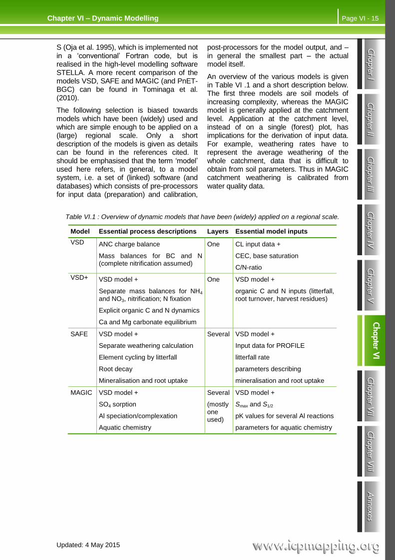
An overview of the various models is given in Table VI .1 and a short description below. The first three models are soil models of increasing complexity, whereas the MAGIC model is generally applied at the catchment level. Application at the catchment level, instead of on a single (forest) plot, has implications for the derivation of input data. For example, weathering rates have to represent the average weathering of the whole catchment, data that is difficult to obtain from soil parameters. Thus in MAGIC catchment weathering is calibrated from water quality data.

Table VI.1 : Overview of dynamic models that have been (widely) applied on a regional scale.

Model Essential process descriptions Layers Essential model inputs

VSD ANC charge balance

Mass balances for BC and N (complete nitrification assumed)

One CL input data +

CEC, base saturation

C/N-ratio

VSD+ VSD model +

Separate mass balances for NH4 and NO3, nitrification; N fixation

Explicit organic C and N dynamics

Ca and Mg carbonate equilibrium

One VSD model +

organic C and N inputs (litterfall, root turnover, harvest residues)

SAFE VSD model +

Separate weathering calculation

Element cycling by litterfall

Root decay

Mineralisation and root uptake

Several VSD model +

Input data for PROFILE

litterfall rate

parameters describing

mineralisation and root uptake

MAGIC VSD model +

SO4 sorption

Al speciation/complexation

Aquatic chemistry

Several

(mostly one used)

VSD model +

Smax and S1/2

pK values for several Al reactions

parameters for aquatic chemistry

Updated: 4 May 2015


VI.3.1 THE VSD MODEL

The basic equations presented in section VI.2 have been used to construct a Very Simple Dynamic (VSD) soil acidification model. The VSD model is designed as the simplest extension of the SMB model for critical loads. In addition to the equations included in the SMB model, it includes cation exchange and N immobilisation as well as a mass balance for cations and nitrogen as described above. It resembles the model presented by Reuss (1980) which, however, does not consider nitrogen processes. The model is described in Posch and Reinds (2009) and a single-site version is available from the CCE website (www.wge-cce.org).

The VSD model consists of a set of mass balance equations, describing the soil input-output relationships, and a set of equations describing the rate-limited and equilibrium soil processes, as described in section VI.2. The soil solution chemistry in VSD depends solely on the net element input from the atmosphere (deposition minus net uptake

minus net immobilisation) and the geochemical interaction in the soil (CO2 equilibria, weathering of carbonates and silicates, and cation exchange). Soil interactions are described by simple rate-limited (zero-order) reactions (e.g. uptake and silicate weathering) or by equilibrium reactions (e.g. cation exchange). It models the exchange of Al, H and Ca+Mg+K with Gaines-Thomas or Gapon equations. Solute transport is described by assuming complete mixing of the element input within one homogeneous soil compartment with a constant density and a fixed depth. Since VSD is a single layer soil model neglecting vertical heterogeneity, it predicts the concentration of the soil water leaving this layer (the rootzone). The annual water flux percolating from this layer is taken equal to the annual precipitation excess. The time step of the model is one year, i.e. seasonal variations are not considered.

VI.3.2 THE VSD+ MODEL

The VSD+ model (Bonten et al. 2015) is an extension of the VSD model. An explicit description of organic C and N turnover has been included to better predict N eutrophication and C sequestration and be able to link the model to vegetation biodiversity models. For C sequestration, VSD+ uses the equations of the RothC-26.3 model (Coleman and Jenkinson 2005). This model consists of five soil C pools. Two pools contain fresh organic input from litterfall, root turnover and harvest residues, whereby one of these pools assembles easily decomposable plant material and the other pool stands for recalcitrant material. For the three other pools, one resembles soil microbial C, one is humified material and the last one is inert organic material. Mineralisation and transfer of C to a next pool is described by single order differential equations, with a fixed reference rate constant for each pool that is adjusted for temperature and soil moisture. Nitrogen mineralization and immobilization follows the turnover of the C pools, depending on the C:N ratios of the five organic matter compartments. The C:N ratio of the pool with easily decomposable

plant material depends on the C:N ratio of the total organic C input. The C:N ratio of the humified pool is adjusted depending on N deposition, N uptake and transfer of N from other pools. The C:N ratios for the three other pools are fixed. Input for this explicit C and N model are the total organic C and N inputs.

Also different from the VSD model, the VSD+ model no longer assumes full nitrification, but includes a first order differential equation for nitrification. Also denitrification is modelled with a first order equation. Nitrification and denitrification rates are calculated from reference rate constants that are modified for temperature, soil moisture and soil pH.

The final difference with VSD is that VSD+ includes equations for Ca and/or Mg carbonates equilibrium, which allows VSD+ to be easier used for calcareous soils, especially for N eutrophication effects (acidification doesn’t not play a big role for these soils).

http://www.wge-cce.orge/

Updated: 4 May 2015


VI.3.3 THE SAFE MODEL

The SAFE (Soil Acidification in Forest Ecosystems) model has been developed at the University of Lund (Warfvinge et al. 1993) and a recent description of the model can be found in Alveteg (1998) and Alveteg and Sverdrup (2002). The main differences to the VSD/VSD+ and MAGIC models are: (a) weathering of base cations is not a model input, but it is modelled with the PROFILE (sub-)model, using soil mineralogy as input (Warfvinge and Sverdrup 1992); (b) SAFE is oriented to soil profiles in which water is assumed to move vertically through several soil layers (usually 4), (c) Cation exchange between Al, H and (divalent) base cations is

modelled with Gapon exchange reactions, and the exchange between soil matrix and the soil solution is diffusion limited. The standard version of SAFE does not include sulphate adsorption although a version, in which sulphate adsorption is dependent on sulphate concentration and pH has been developed (Martinson et al. 2003).

The SAFE model has been applied to many sites and more recently also regional applications have been carried out for Sweden (Alveteg and Sverdrup 2002) and Switzerland (SAEFL 1998, Kurz et al. 1998, Alveteg et al. 1998).

VI.3.4 THE MAGIC MODEL

MAGIC (Model of Acidification of Groundwater In Catchments) is a lumped-parameter model of intermediate complexity, developed to predict the long-term effects of acidic deposition on soils and surface water chemistry (Cosby et al. 1985a,b,c, 1986). The model simulates soil solution chemistry and surface water chemistry to predict the monthly and annual average concentrations of the major ions in lakes and streams. MAGIC represents the catchment with aggregated, uniform soil compartments (one or two) and a surface water compartment that can be either a lake or a stream. MAGIC consists of (1) a section in which the concentrations of major ions are assumed to be governed by simultaneous reactions involving sulphate adsorption, cation exchange, dissolution-precipitation-speciation of aluminium and dissolution-speciation of inorganic and organic carbon, and (2) a mass balance section in which the flux of major ions to and from the soil is assumed to be controlled by atmospheric inputs, chemical weathering inputs, net uptake in biomass and losses to runoff. At the heart of MAGIC is the size of the pool of exchangeable base cations in the soil. As the fluxes to and from this pool change over time owing to changes in atmospheric deposition, the chemical equilibria between soil and soil solution shift to give changes in surface water chemistry. The degree and rate of change in surface water acidity thus depend both on flux factors and the

inherent characteristics of the affected soils.

The soil layers can be arranged vertically or horizontally to represent important vertical or horizontal flowpaths through the soils. If a lake is simulated, seasonal stratification of the lake can be implemented. Time steps are monthly or yearly. Time series inputs to the model include annual or monthly estimates of: (1) deposition (wet plus dry) of ions from the atmosphere; (2) discharge volumes and flow routing within the catchment; (3) biological production, removal and transformation of ions; (4) internal sources and sinks of ions from weathering or precipitation reactions; and (5) climate data. Constant parameters in the model include physical and chemical characteristics of the soils and surface waters, and thermodynamic constants. The model is calibrated using observed values of surface water and soil chemistry for a specified period.

MAGIC has been modified and extended several times from the original version of 1984. In particular organic acids have been added to the model (version 5; Cosby et al. 1995a), nitrogen processes have been added based on the C/N ratio of soil (version 7; Cosby et al. 2001) and most recently N retention in soil is described as a microbial-driven process (i.e. the C/N ratio of the soil no longer governs the N immobilisation) (Oulehle et al., 2012).

Updated: 4 May 2015


The MAGIC model has been extensively applied and tested over the past 30 years at many sites and in many regions around

the world. Overall, the model has proven to be robust, reliable and useful in a variety of scientific and managerial activities.

VI.4 INPUT DATA AND MODEL CALIBRATION

Running a dynamic model is usually the least time- or resource-consuming step in an assessment. It takes time to interpret model output, but most time-consuming is the acquisition and preparation of input data. Rarely can field, laboratory or literature data be directly used as model inputs. They have to be pre-processed and interpreted, often with the help of other models. Especially for regional applications not all model inputs are available (or directly usable) from measurements at sites, and interpolations and transfer functions have to be derived and used to obtain the necessary input data. When acquiring data from different sources of information, it is important to keep a record of the ‘pedigree’, i.e. the entire chain

of information, assumptions and (mental) models used to produce a certain number. Also the uncertainty of the data should be assessed, recorded and communicated.

As with critical loads, for the policy support of the effects-oriented work under the LRTAP Convention, output of dynamic models will most usefully represent not a particular site, but a larger area, e.g. a forest instead of a single tree stand. Therefore, certain variables should be ‘smoothed’ to represent that larger area. For example, (projected) growth uptake of nutrients (nitrogen and base cations) should reflect the (projected) average uptake of the forest over that area, and not the succession of harvest and re-growth at a particular spot.

VI.4.1 INPUT DATA

The input data required to run dynamic models depend on the model, but essentially all of them need the following (minimum) data, which can be roughly grouped into in- and output fluxes, and soil properties. Note that this grouping of the input data depends on the model considered. For example, weathering has to be specified as a (constant) input flux in the VSD/VSD+ models, whereas in the SAFE model it is internally computed from soil properties and depends on the state of the soil (e.g. the pH). Some of the input data are also needed in the SMB model to calculate critical loads, and are described in Chapter V. This chapter thus focuses on additional data and parameters needed to run dynamic models. The most important soil parameters are the cation exchange capacity (CEC), the base saturation and the exchange (or selectivity) constants describing cation exchange, as well as parameters describing nitrogen retention and sulphate ad/desorption, since these parameters determine the long-term behaviour (recovery) of soils.

Ideally, all input data are directly derived from measurements. This is usually not feasible for regional applications, in which case input data have to be derived from

relationships (transfer functions) with basic (map) information. In this chapter, we provide information on the input data needed for running the VSD model and thus, by extension, also other models. Descriptions and technical details of the input data for those models can be found in Posch and Reinds (2009) for the VSD model, in Bonten et al (2015) for the VSD+ model, in Cosby et al. (1985a, 2001) for the MAGIC model and in Alveteg and Sverdrup (2002) for the SAFE model.

In most of the (pedo-)transfer functions presented here, soils – or rather soil groups – are characterised by a few properties, mostly organic carbon and clay content of the mineral soil (see also Figure VI.3) . The organic carbon content, Corg, can be estimated as 0.5 or 0.4 times the organic matter content in the humus or mineral soil layer, resp. If Corg>15%, a soil is considered a peat soil. Mineral soils are called sand (or sandy soil) here, if the clay content is below 18% (coarse textured soils; see also Table VI.6), otherwise it is called a clay (or clayey/loamy soil). Loess soils are soils with more than 50% silt, i.e. clay+sand<50% (since clay+silt+sand=100%).

Updated: 4 May 2015


sand

clay

silt

30%

30%

30%

60%

60%

60%Volume Mass

Water content ( )

Organic carbon (Corg)

100%

100%

Non-C organic matter

Figure VI.3 : Illustration of the basic composition of a soil profile: soil water, organic matter (organic carbon) and the mineral soil, characterised by its clay, silt and sand fraction

(clay+silt+sand=100%).

VI.4.1.1 AVERAGING SOIL PROPERTIES

For single layer soil models, such as VSD, VSD+ or MAGIC, the profile averages of certain soil parameters are required, and in the sequel formulae for the average bulk density, cation exchange capacity and base saturation are derived.

For a given soil profile it is assumed that

there are measurements of bulk density l (g/cm3), cation exchange capacity CECl (meq/kg) and base saturation EBC,l for n (homogeneous) soil horizons with thickness zl (l=1,..., n). Obviously, the total thickness (soil depth) z is given by:

(VI.21)

n

l

lzz1

The mean bulk density ρ of the profile is derived from mass conservation (per unit area):

(VI.22)

n

l

llzz 1

1

The average cation exchange capacity CEC has to be calculated in such a way that the total number of exchange sites (per unit

area) is given by zCEC. This implies the following formula for the profile average cation exchange capacity:

(VI.23)

n

l

lll CECzz

CEC1

1

And for the profile average base saturation EBC one then gets:

(VI.24)

n

l

lBClllBC ECECzCECz

E1

,

1

Note that for aquatic ecosystems, these parameters have to be averaged over the terrestrial catchment area as well.

VI.4.1.2 DATA ALSO USED FOR CRITICAL LOAD CALCULATIONS

In this section we describe those input data which are also used in critical load calculations (see Chapter V) and for details the reader is referred to that Chapter, especially sections V.3.1.3 and V.3.2.3.

Whereas for critical loads and exceedance calculations data are needed at a specific point in time (or at steady state), their past and future temporal development is needed for dynamic modelling.

Updated: 4 May 2015


VI.4.1.2.1 DEPOSITION

Non-anthropogenic (steady-state) base cation and chloride deposition are incorporated into the definition of the critical load of acidity. For dynamic models times, series of past and future depositions are needed. However, at present there are no projections available for these elements on a European scale. Thus in most model applications (average) present base cation and chloride depositions are assumed to hold also in the future (and past).

Sulphur and nitrogen depositions enter only the exceedance calculations of critical loads. In contrast, their temporal development is the driving force of every dynamic model. Time series for the period 1880–1990 of S and N deposition on the EMEP-150 grid have been computed using published estimates of historical emissions (Schöpp et al. 2003) and 12-year average transfer matrices derived from the EMEP/MSC-W

lagrangian atmospheric transport model. Equivalent datasets have been prepared for the EMEP 50x50 km2 as well as the latest 10x10 km2 grids.

Scenarios for future sulphur and nitrogen deposition are provided by integrated assessment modellers, based on atmospheric transport modelling by EMEP.

In case the deposition model provides only grid average values, a local deposition (adjustment) model could compute the local deposition from the grid average values, especially for forest soils, where the actual (larger) deposition depends on the type and age of trees (via the ‘filtering’ of deposition by the canopy). An example of such a model is the MAKEDEP model, which is also part of the SAFE model system (Alveteg and Sverdrup 2002).

VI.4.1.2.2 UPTAKE

Long-term average values of the net growth-uptake of nitrogen and base cations by forests are also needed to calculate critical loads. Data sources and calculation procedures are given in Chapter V. In simple dynamic models these processes are described as a function of actual and projected forest growth. To this end, additional information on forest age and growth rates is needed, and the amount of data needed depends largely on whether the full nutrient cycle is modelled or whether only net sources and sinks are considered.

Considering net removal by forest growth, as in the VSD and MAGIC models, the yield

(forest growth) at a certain age can be derived from yield tables for the considered tree species. The element contents in stems (and possibly branches) should be the same as used in the critical load calculations (see, e.g., Table V.2). If the nutrient cycle is modelled, as in the SAFE model, data are needed on litterfall rates, root turnover rates, including the nutrient contents in litter (leaves/needles falling from the tree), and fine roots. Such data are highly dependent on tree species and site conditions. Compilations of such data can be found in De Vries et al. (1990) and Jacobsen et al. (2002).

VI.4.1.2.3 WATER FLUX AND SOIL MOISTURE

Water flux data that are needed in one-layer models are limited to the precipitation surplus leaving the root zone (see Chapter V), whereas multi-layer models require water fluxes for each soil layer down to the bottom of the root zone. For simple dynamic models, water fluxes could be calculated by a separate hydrological model, running on a daily or monthly time step with aggregation to annual values afterwards. An example of such a model is WATBAL

(Starr 1999), which is a capacity-type water balance model for forested stands/plots running on a monthly time step and based on the following water balance equation:

(VI.25) SMETPQ

where Q = precipitation surplus, P = precipitation, ET= evapotranspiration and

±SM = changes in soil moisture content. WATBAL uses relatively simple input data, which is either directly

Updated: 4 May 2015


available (e.g., monthly precipitation and air temperature) or which can be derived from other data using transfer functions (e.g., soil available water capacity).

In any dynamic model, which includes a mass balance for elements, also information on the soil moisture content is needed. This is also output from a hydrological model (see SM in eq.6.25) or has to be estimated from other site properties. An approximate annual

average soil moisture content θ (m3/m3) can be obtained as a function of the clay content (see Brady 1974):

(VI.26)

27.0,0077.004.0min clay

i.e., for clay contents above 30% a constant value of 0.27 is assumed. It should be noted that most models are quite insensitive to the value of θ.

VI.4.1.2.4 BASE CATION WEATHERING

The various possibilities to assess weathering rates of base cations, which are a key input also to critical load calculations, are discussed and cited in Chapter V.

VI.4.1.2.5 MINERALISATION AND (DE-)NITRIFICATION

Rate constants (and possibly additional parameters) for mineralisation, nitrification and denitrification are needed in detailed models, but simple models mostly use factors between zero and one, which compute nitrification and denitrification as fraction of the (net) input of nitrogen.

As in the calculation of critical loads (SMB model), in the VSD model complete nitrification is assumed (nitrification fraction equals 1.0), and denitrification fractions can be found in Table V.3. Mineralisation is not considered explicitly, but included in the net immobilisation calculations.

For the complete soil profile, the nitrification fraction in forest soils varies mostly between 0.75 and 1.0. This is based on measurements of NH4/NO3 ratios below the root-zone of highly acidic Dutch forests with very high NH4 inputs in the early nineties, which were nearly always less than 0.25 (De Vries et al. 1995). Generally, 50% of the NH4 input is nitrified above the mineral soil in the humus layer (Tietema et al. 1990). Actually, the nitrification fraction includes the effect of both nitrification and preferential ammonium uptake.

VI.4.1.2.6 AL-H EQUILIBRIUM

The constants needed to quantify the equilibrium between [Al] and [H] in the soil solution are discussed and presented in Chapter V (Table V.9), since they are also needed for critical load calculations. For

models including the complexation of Al with organic anions, such as MAGIC, relevant parameters can be found, e.g., in Driscoll et al. (1994).

VI.4.1.3 DATA NEEDED TO SIMULATE CATION EXCHANGE

In all dynamic soil models, cation exchange is a crucial process (see section VI.2.3.1). Data needed to allow exchange calculations are:

The pool of exchangeable cations, being the product of layer thickness, bulk density, cation exchange capacity (CEC) and exchangeable cation fractions

Cation exchange constants (selectivity coefficients)

Preferably these data are taken from measurements. Such measurements are generally made for several soil horizons. For single-layer models, such as VSD, these data have to be properly averaged over the entire soil depth (rooting zone; see eqs. VI.21 – VI.24).

In the absence of measurements, the various data needed to derive the pool of exchangeable cations for major forest soil types can be derived by extrapolation of point data, using transfer functions

Updated: 4 May 2015


between bulk density, CEC and base saturation and basic land and soil characteristics, such as soil type, soil

horizon, organic matter content, soil texture, etc.

VI.4.1.3.1 SOIL BULK DENSITY

If no measurements are available, the soil bulk density ρ (g cm-3) can be estimated from the following transfer function:

(VI.27)

%15forlog337.0725.0

%15%5for0814.055.1

%5for0015.005.0625.0/1

10 orgorg

orgorg

orgorg

CC

CC

CclayC

where Corg is the organic carbon content and clay the clay content (both in %). The top equation for mineral soils is based on data by Hoekstra and Poelman (1982), the bottom equation for peat(y) soils is derived from Van Wallenburg (1988) and the central equation is a linear interpolation (for clay=0) between the two.

VI.4.1.3.2 CATION EXCHANGE CAPACITY (CEC)

The value of the CEC depends on the soil pH at which the measurements are made. Consequently, there is a difference between unbuffered CEC values, measured at the actual soil pH and buffered values measured at a standard pH, such as 6.5 or 8.2. In the VSD (and many other) models the exchange constants are related to a CEC that is measured in a buffered solution in order to standardise to a single pH value (e.g., pH=6.5, as upper limit of non-calcareous soils). The actual CEC can be calculated from pH, clay and organic carbon content according to (after Helling et al. 1964):

(VI.28)

orgCpHclaypHpHCEC )9.51.5()0.344.0()(

where CEC is the cation exchange capacity (meq/kg), clay is the clay content (%) and Corg the organic carbon content (%). The pH in this equation should be as close as possible to the measured soil solution pH. For sandy soils the clay content can be set to zero in eq. VI.28. Typical average clay contents as a function of the texture class, presented on the FAO soil classification (FAO 1981), are given in Table VI.2. Values for Corg range from 0.1% for arenosols (Qc) to 50% for peat soils (Od).

Table VI.2 : Average clay contents and typical base saturation as a function of soil texture classes (see Table VI.6).

Texture class

Name Definition Average

clay content (%)

Typical

base saturation (%)

1 coarse clay < 18% and sand 65% 6 5

2 medium clay < 35% and sand 15%;

but clay 18% if sand 65%

20 15

3 medium fine clay < 35% and sand < 15% 20 20

4 fine 35% clay < 60% 45 50

5 very fine clay 60% 75 50

9 organic soils Soil types O 5 10-70

Updated: 4 May 2015


Computing CEC(pHmeasured), i.e. the CEC from eq. VI.28, using measured (site-specific) Corg, clay and pH does not always match the measured CEC, CECmeasured, and thus computing CEC at pH=6.5, CEC(6.5), would not be consistent with it. Nevertheless, eq. VI.28 can be used to scale the measured CEC to a value at pH=6.5, i.e. the value needed for modelling, in the following manner:

(VI.29)

)(

)5.6(5.6

measuredpHCEC

CECmeasuredpH CECCEC

This method of scaling measured data with the ratio (or difference) of model output is widely used in global change work to obtain, e.g., climate-changed (meteorological) data consistent with observations.

VI.4.1.3.3 EXCHANGEABLE BASE CATION FRACTION (BASE

SATURATION)

In most models, a lumped expression is used for the exchange of cations, distinguishing only between H, Al and base cations (VSD, VSD+ and SAFE). As with the clay content, data for the exchangeable cation fractions, or in some cases only the base saturation, can be based on information on national soil information systems, or in absence of these, on the FAO soil map of Europe (FAO 1981). Base saturation data vary from 5-25% in relatively acid forest soils to more than 50% in well buffered soils. A very crude indication of the base saturation as a function of the texture class of soils is given in the last column of Table VI.2. This relationship is based on data from forest soils given in FAO (1981) and in Gardiner (1987). A higher texture class reflects a higher clay content implying an increase in weathering rate, which implies a higher

base saturation. For organic soils the base saturation is put equal to 70% for eutric histosols (Oe) and 10% for dystric histosols (Od).

Ideally, only measured CEC and exchangeable cation data are used. However, when data on the initial base saturation of soils are not available for regional (national) model applications, one may derive them from a relationship with environmental factors. Such an exercise was carried out using a European database with approximately 5300 soil chemistry data for the organic layer and the forest topsoil (0-20 cm) collected on a systematic 16×16 km2 grid (ICP Forest level-I grid; Vanmechelen et al. 1997). The regression relationship for the estimated base saturation EBC (expressed as a fraction with values between 0 and 1) is:

(VI.30a) BBCE

e1

1

with

(VI.30b)

15

12

11

8

7

2

65

43210

)fractiondepositionlt()depositionln(

)ionprecipitatln()etemperatur(etemperatur

)ageln(altitude)speciestree()groupsoil(

k

k kk

k

k kk aa

aaa

aaaaaB

where ‘ln’ is the natural logarithm, lt(x)=ln(x/(1–x)), and the ak’s are the regression coefficients. The regression analysis was carried out using a so-called Select-procedure. This procedure combines qualitative predictor variables, such as tree species and/or soil type, with quantitative variables and it combines forward selection, starting with a model including one predictor variable, and backward elimination, starting with a model

including all predictor variables. The ‘best’ model was based on a combination of the percentage of explained variance, that should be high and the number of predictor variables that should be low. More information on the procedure is given in Klap et al. (2004). Results of the analyses are given in Table VI.3. The explained variance for base saturation was approx. 45%.

Updated: 4 May 2015


Note: When data are not available, one may also calculate base saturation as the maximum of (i) a relation with environmental factors as given above and (ii) an equilibrium with present deposition levels of SO4, NO3, NH4 and BC. Especially

in southern Europe, where acid deposition is relatively low and base cation input is high, the base saturation in equilibrium with the present load can be higher than the value computed according to eq. VI.30.

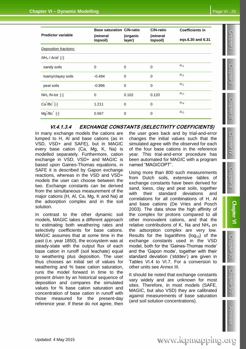
Table VI.3 : Coefficients for estimating base saturation and the C/N-ratio in the mineral topsoil (0-20cm) and the organic layer (after Klap et al. 2004; Note: (a) the star denotes sea-salt corrected

depositions, (b) depositions<0.1 should be set to 0.1 to avoid underflow in the equations).

Predictor variable

Base saturation

(mineral topsoil)

C/N-ratio

(organic layer)

C/N-ratio

(mineral topsoil)

Coefficients in

eqs.6.30 and 6.31

Constant 3.198 3.115 1.310 a0

Soil group:

sandy soils 0 0 0 a1

loamy/clayey soils 0.297 -0.807 -0.279 a1

peat soils 0.534 -0.025 -0.312 a1

Tree species:

pine 0 0 0 a2

spruce -0.113 -0.158 -0.093 a2

oak 0.856 -0.265 -0.218 a2

beech 0.591 -0.301 -0.218 a2

Site conditions:

Altitude [m] -0.00014 -0.00008 -0.000136 a3

Age [yr] 0 0.025 0.096 a4

Meteorology:

Temperature [C] 0 -0.0078 -0.041 a5

Temperature2 [C

2] 0 0.00095 0.0014

a6

Precipitation [mm/yr] 0 0.178 0.194 a7

Deposition:

Na [eq/ha/yr] -0.223 0 0.080 a8

N-tot (=NOy+NHz) [eq/ha/yr]:

sandy soils 0 -0.150 -0.019 a9

loamy/clayey soils 0 -0.032 0 a9

peat soils 0 -0.136 0 a9

Acid (=SOx*+N-tot) [eq/ha/yr] -1.025 0 0

a10

Bc* (=Ca

*+Mg

*+K

*) [eq/ha/yr] 0.676 0 0

a11

Updated: 4 May 2015


Predictor variable

Base saturation

(mineral topsoil)

C/N-ratio

(organic layer)

C/N-ratio

(mineral topsoil)

Coefficients in

eqs.6.30 and 6.31

Deposition fractions:

NHz / Acid [-]:

sandy soils 0 0 0 a12

loamy/clayey soils -0.494 0 0 a12

peat soils -0.896 0 0 a12

NHz /N-tot [-] 0 0.102 0.120 a13

Ca*/Bc

* [-] 1.211 0 0

a14

Mg*/Bc

* [-] 0.567 0 0

a15

VI.4.1.3.4 EXCHANGE CONSTANTS (SELECTIVITY COEFFICIENTS)

In many exchange models the cations are lumped to H, Al and base cations (as in VSD, VSD+ and SAFE), but in MAGIC every base cation (Ca, Mg, K, Na) is modelled separately. Furthermore, cation exchange in VSD, VSD+ and MAGIC is based upon Gaines-Thomas equations, in SAFE it is described by Gapon exchange reactions, whereas in the VSD and VSD+ models the user can choose between the two. Exchange constants can be derived from the simultaneous measurement of the major cations (H, Al, Ca, Mg, K and Na) at the adsorption complex and in the soil solution.

In contrast to the other dynamic soil models, MAGIC takes a different approach to estimating both weathering rates and selectivity coefficients for base cations. MAGIC assumes that at some time in the past (i.e. year 1850), the ecosystem was at steady-state with the output flux of each base cation in runoff (soil leachate) equal to weathering plus deposition. The user thus chooses an initial set of values for weathering and % base cation saturation, runs the model forward in time to the present driven by an historical sequence of deposition and compares the simulated values for % base cation saturation and concentration of base cation in runoff with those measured for the present-day reference year. If these do not agree, then

the user goes back and by trial-and-error changes the initial values such that the simulated agree with the observed for each of the four base cations in the reference year. This trial-and-error procedure has been automated for MAGIC with a program named “MAGICOPT”.

Using more than 800 such measurements from Dutch soils, extensive tables of exchange constants have been derived for sand, loess, clay and peat soils, together with their standard deviations and correlations for all combinations of H, Al and base cations (De Vries and Posch 2003). The data show the high affinity of the complex for protons compared to all other monovalent cations, and that the relative contributions of K, Na and NH4 on the adsorption complex are very low. Results for the logarithms (log10) of the exchange constants used in the VSD model, both for the ‘Gaines-Thomas mode’ and the ‘Gapon mode’, together with their standard deviation (‘stddev’) are given in Tables VI.4 to VI.7. For a conversion to other units see Annex III.

It should be noted that exchange constants vary widely and are unknown for most sites. Therefore, in most models (SAFE, MAGIC, but also VSD) they are calibrated against measurements of base saturation (and soil solution concentrations).

Updated: 4 May 2015


Table VI.4 : Mean and standard deviation of logarithmic Gaines-Thomas exchange constants of H against Ca+Mg+K as a function of soil depth for sand, loess, clay and peat soils (mol/l)

–1.

Layer Sand Loess Clay Peat

(cm) Mean stddev Mean Stddev Mean stddev Mean stddev

0-10 5.338 0.759 5.322 0.692 6.740 1.464 4.754 0.502

10-30 6.060 0.729 5.434 0.620 6.007 0.740 4.685 0.573

30-60 6.297 0.656 - - 6.754 0.344 5.307 1.051

60-100 6.204 0.242 5.541 0.579 7.185 - 5.386 1.636

0-30 5.236 0.614 5.386 0.606 6.728 1.373 4.615 0.439

0-60 5.863 0.495 - - 6.887 1.423 4.651 0.562

Table VI.5 : Mean and standard deviation of logarithmic Gaines-Thomas exchange constants of Al against Ca+Mg+K as a function of soil depth for sand, loess, clay and peat soils (mol/l).



0-10 2.269 1.493 1.021 1.147 1.280 1.845 0.835 1.204

10-30 3.914 1.607 1.257 0.939 -0.680 1.152 0.703 0.968

30-60 4.175 1.969 - - -3.070 0.298 0.567 1.474

60-100 2.988 0.763 1.652 1.082 -2.860 - 0.969 1.777

0-30 2.306 1.082 0.878 1.079 0.391 1.555 0.978 0.805

0-60 2.858 1.121 - - -0.973 1.230 0.666 0.846

Table VI.6 : Mean and standard deviation of logarithmic Gapon exchange constants of H against Ca+Mg+K as a function of soil depth for sand, loess, clay and peat soils (mol/l)

–1/2.



0-10 3.178 0.309 3.138 0.268 3.684 0.568 2.818 0.199

10-30 3.527 0.271 3.240 0.221 3.287 0.282 2.739 0.175

30-60 3.662 0.334 - - 3.521 0.212 2.944 0.382

60-100 3.866 0.125 3.232 0.251 3.676 - 3.027 0.672

0-30 3.253 0.311 3.170 0.206 3.620 0.530 2.773 0.190

0-60 3.289 0.340 - - 3.604 0.654 2.694 0.170

Updated: 4 May 2015


Table VI.7 : Mean and standard deviation of logarithmic Gapon exchange constants of Al against Ca+Mg+K as a function of soil depth for sand, loess, clay and peat soils (mol/l)

1/6.



0-10 0.306 0.440 0.190 0.546 -0.312 0.738 -0.373 0.350

10-30 0.693 0.517 0.382 0.663 -0.463 0.431 -0.444 0.255

30-60 0.819 0.527 - - -1.476 0.093 -0.740 0.336

60-100 1.114 0.121 0.390 0.591 -1.795 - -0.867 0.401

0-30 0.607 0.472 0.221 0.647 -0.609 0.731 -0.247 0.404

0-60 0.199 0.633 - - -1.054 0.362 -0.551 0.210

VI.4.1.4 DATA NEEDED FOR BALANCES OF NITROGEN, SULPHATE AND

ALUMINIUM

VI.4.1.4.1 C/N-RATIO

Data for the C/N-ratio generally vary between 15 in rich soils where humification has been high to 40 in soils with low N inputs and less humification. Values can

also be obtained from results of a regression analysis similar to that of the base saturation according to:

(VI.31)

15

12

11

8

72

65

43210

)fractiondepositionlt()depositionln(

)ionprecipitatln()etemperatur(etemperatur

)ageln(altitude)speciestree()groupsoil(ratio-C/Nln

k

k kk

k

k kk aa

aaa

aaaaa

where ‘ln’ is the natural logarithm and lt(x) = ln(x/(1–x)). Results of the analysis, which was performed with the same data sets as described in the section on base saturation,

are given in Table VI.3; and more information on the procedure is given in Klap et al. (2004).

VI.4.1.4.2 SULPHATE SORPTION CAPACITY AND HALF-

SATURATION CONSTANT

Values for the maximum sorption capacity for sulphate, Smax, can be related to the content of oxalate extractable Al (meq kg-1) according to (Johnson and Todd 1983):

(VI.32) oxmax AlS 02.0

Estimates for the oxalate extractable Al content are given below. Adsorption or half-saturation constants for sulphate, S1/2, can be derived from literature information (e.g. Singh and Johnson 1986, Foster et al. 1986). A reasonable average value is 1.0 eq/m3.

VI.4.1.4.3 AL-HYDROXIDE CONTENT

Data for the oxalate extractable Al content (the content of readily available Al-hydroxide) are often available in national soil information systems, such as the soil information system of the Netherlands. In

sandy soils the Al-hydroxide content (in meq/kg) mostly varies between 100-200 for A-horizons, between 200-350 for B-horizons and between 50-150 for C-horizons (parent material, De Vries 1991).

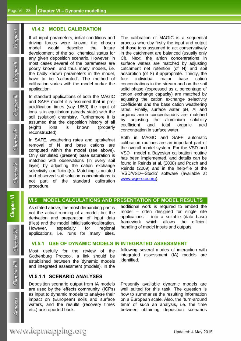
Updated: 4 May 2015


VI.4.2 MODEL CALIBRATION

If all input parameters, initial conditions and driving forces were known, the chosen model would describe the future development of the soil chemical status for any given deposition scenario. However, in most cases several of the parameters are poorly known, and thus many models, i.e. the badly known parameters in the model, have to be ‘calibrated’. The method of calibration varies with the model and/or the application.

In standard applications of both the MAGIC and SAFE model it is assumed that in pre-acidification times (say 1850) the input of ions is in equilibrium (steady state) with the soil (solution) chemistry. Furthermore it is assumed that the deposition history of all (eight) ions is known (properly reconstructed).

In SAFE, weathering rates and uptake/net removal of N and base cations are computed within the model (see above). Only simulated (present) base saturation is matched with observations (in every soil layer) by adjusting the cation exchange selectivity coefficient(s). Matching simulated and observed soil solution concentrations is not part of the standard calibration procedure.

The calibration of MAGIC is a sequential process whereby firstly the input and output of those ions assumed to act conservatively in the catchment are balanced (usually only Cl). Next, the anion concentrations in surface waters are matched by adjusting catchment net retention (of N) and soil adsorption (of S) if appropriate. Thirdly, the four individual major base cation concentrations in the stream and on the soil solid phase (expressed as a percentage of cation exchange capacity) are matched by adjusting the cation exchange selectivity coefficients and the base cation weathering rates. Finally, surface water pH, Al and organic anion concentrations are matched by adjusting the aluminium solubility coefficient and total organic acid concentration in surface water.

Both in MAGIC and SAFE automatic calibration routines are an important part of the overall model system. For the VSD and VSD+ model a Bayesian calibration routine has been implemented, and details can be found in Reinds et al. (2008) and Posch and Reinds (2009) and in the help-file of the ‘VSD/VSD+-Studio’ software (available at www.wge-cce.org).

VI.5 MODEL CALCULATIONS AND PRESENTATION OF MODEL RESULTS

As stated above, the most demanding part is not the actual running of a model, but the derivation and preparation of input data (files) and the model initialisation/calibration. However, especially for regional applications, i.e. runs for many sites,

additional work is required to embed the model – often designed for single site applications – into a suitable (data base) framework which allows the efficient handling of model inputs and outputs.

VI.5.1 USE OF DYNAMIC MODELS IN INTEGRATED ASSESSMENT

Most usefully for the review of the Gothenburg Protocol, a link should be established between the dynamic models and integrated assessment (models). In the

following several modes of interaction with integrated assessment (IA) models are identified.

VI.5.1.1 SCENARIO ANALYSES

Deposition scenario output from IA models are used by the ‘effects community’ (ICPs) as input to dynamic models to analyse their impact on (European) soils and surface waters, and the results (recovery times etc.) are reported back.

Presently available dynamic models are well suited for this task. The question is how to summarise the resulting information on a European scale. Also, the ‘turn-around time’ of such an analysis, i.e. the time between obtaining deposition scenarios

http://www.wge-cce.org/

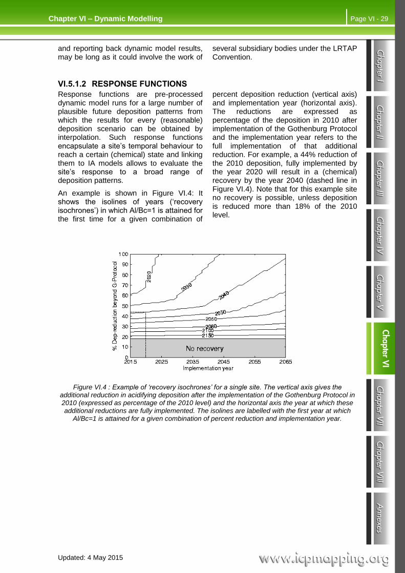
Updated: 4 May 2015


and reporting back dynamic model results, may be long as it could involve the work of

several subsidiary bodies under the LRTAP Convention.

VI.5.1.2 RESPONSE FUNCTIONS

Response functions are pre-processed dynamic model runs for a large number of plausible future deposition patterns from which the results for every (reasonable) deposition scenario can be obtained by interpolation. Such response functions encapsulate a site’s temporal behaviour to reach a certain (chemical) state and linking them to IA models allows to evaluate the site’s response to a broad range of deposition patterns.

An example is shown in Figure VI.4: It shows the isolines of years (‘recovery isochrones’) in which Al/Bc=1 is attained for the first time for a given combination of

percent deposition reduction (vertical axis) and implementation year (horizontal axis). The reductions are expressed as percentage of the deposition in 2010 after implementation of the Gothenburg Protocol and the implementation year refers to the full implementation of that additional reduction. For example, a 44% reduction of the 2010 deposition, fully implemented by the year 2020 will result in a (chemical) recovery by the year 2040 (dashed line in Figure VI.4). Note that for this example site no recovery is possible, unless deposition is reduced more than 18% of the 2010 level.

Figure VI.4 : Example of ‘recovery isochrones’ for a single site. The vertical axis gives the additional reduction in acidifying deposition after the implementation of the Gothenburg Protocol in 2010 (expressed as percentage of the 2010 level) and the horizontal axis the year at which these additional reductions are fully implemented. The isolines are labelled with the first year at which

Al/Bc=1 is attained for a given combination of percent reduction and implementation year.

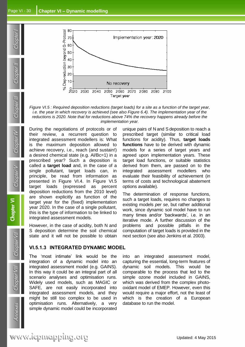
Updated: 4 May 2015


Figure VI.5 : Required deposition reductions (target loads) for a site as a function of the target year, i.e. the year in which recovery is achieved (see also Figure 6.4). The implementation year of the reductions is 2020. Note that for reductions above 74% the recovery happens already before the

implementation year.

During the negotiations of protocols or of their review, a recurrent question to integrated assessment modellers is: What is the maximum deposition allowed to achieve recovery, i.e., reach (and sustain!) a desired chemical state (e.g. Al/Bc=1) in a prescribed year? Such a deposition is called a target load and, in the case of a single pollutant, target loads can, in principle, be read from information as presented in Figure VI.4. In Figure VI.5 target loads (expressed as percent deposition reductions from the 2010 level) are shown explicitly as function of the target year for the (fixed) implementation year 2020. In the case of a single pollutant, this is the type of information to be linked to integrated assessment models.

However, in the case of acidity, both N and S deposition determine the soil chemical state and it will not be possible to obtain

unique pairs of N and S deposition to reach a prescribed target (similar to critical load functions for acidity). Thus, target loads functions have to be derived with dynamic models for a series of target years and agreed upon implementation years. These target load functions, or suitable statistics derived from them, are passed on to the integrated assessment modellers who evaluate their feasibility of achievement (in terms of costs and technological abatement options available).

The determination of response functions, such a target loads, requires no changes to existing models per se, but rather additional work, since dynamic soil model have to run many times and/or ‘backwards’, i.e. in an iterative mode. A further discussion of the problems and possible pitfalls in the computation of target loads is provided in the next section (see also Jenkins et al. 2003).

VI.5.1.3 INTEGRATED DYNAMIC MODEL

The ‘most intimate’ link would be the integration of a dynamic model into an integrated assessment model (e.g. GAINS). In this way it could be an integral part of all scenario analyses and optimisation runs. Widely used models, such as MAGIC or SAFE, are not easily incorporated into integrated assessment models, and they might be still too complex to be used in optimisation runs. Alternatively, a very simple dynamic model could be incorporated

into an integrated assessment model, capturing the essential, long-term features of dynamic soil models. This would be comparable to the process that led to the simple ozone model included in GAINS, which was derived from the complex photo-oxidant model of EMEP. However, even this would require a major effort, not the least of which is the creation of a European database to run the model.

Updated: 4 May 2015


VI.5.2 TARGET LOAD CALCULATIONS

As outlined above, target loads, or target load functions in the case of acidification, are a way to link dynamic models with integrated assessment models, not least due to their similarity with critical load functions (see Chapter V). If a target load exists, there exist also an infinite variety of deposition paths to reach that target load. To bring order into this multitude and to make results comparable, we define a target load as a deposition path characterised by three numbers (years): (i) the protocol year, (ii) the implementation year, and (iii) the target year (see Figure 6.6). If needed, these terms are proceeded by the term ‘dynamic modelling’ (‘DM’) to distinguish them from similar terms used in integrated assessment circles.

In contrast to scenario analyses, the computation of target loads is not straightforward. After specifying the target year and the year of implementation of the (yet unknown) target load, the dynamic model has to be run iteratively until the deposition (= target load) is found which is required to reach the desired chemical status in the specified target year. The following examples demonstrate the different cases that can arise when calculating target

loads and what can happen when doing such calculations ‘blindly’. For simplicity we use a single pollutant (deposition), but the conclusions hold for target load functions as well.

As an example, Figure VI.7 shows the deposition history (left) and the resulting molar Al/Bc-ratio (right) as simulated (by the VSD model) for three different soils, solely distinguished by their CEC (40, 60 and 80 meq/kg). In two cases the Al/Bc-ratio in the year 2010 is above the critical value (=1), while for CEC=80 it stayed below it during the past. To investigate the future behaviour of the soils, we let the deposition drop to the critical load (which is independent of the CEC) during the ‘implementation period’ (marked by two vertical lines in Figure VI.7). Obviously, for CEC=80, the Al/Bc-ratio stays below one, whereas for CEC=60 it drops below one within the first decade and then slowly rises again towards the critical value. For CEC=40, the Al/Bc-ratio stays well above the critical value, approaching it asymptotically over time. In all three cases the approach to the critical value is very slow.

1960 1980 2000 2040 20602020

protocol year

DM implementation year

DM target year 1 DM target year 2

De

po

sitio

n

1960 1980 2000 2040 20602020

protocol year

DM implementation year

DM target year 1 DM target year 2

De

po

sitio

n

Figure VI.6 :Deposition paths for calculating target loads by dynamic models (DM) are characterised by three key years. (i) The year up to which the (historic) deposition is fixed

(protocol year); (ii) the year in which the emission reductions leading to a target load are fully implemented (DM implementation year); and (iii) the years in which the chemical criterion is to be

achieved (DM target years).

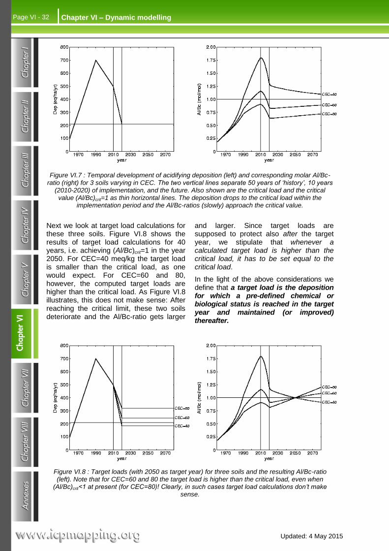
Updated: 4 May 2015


Figure VI.7 : Temporal development of acidifying deposition (left) and corresponding molar Al/Bc-ratio (right) for 3 soils varying in CEC. The two vertical lines separate 50 years of ‘history’, 10 years

(2010-2020) of implementation, and the future. Also shown are the critical load and the critical value (Al/Bc)crit=1 as thin horizontal lines. The deposition drops to the critical load within the

implementation period and the Al/Bc-ratios (slowly) approach the critical value.

Next we look at target load calculations for these three soils. Figure VI.8 shows the results of target load calculations for 40 years, i.e. achieving (Al/Bc)crit=1 in the year 2050. For CEC=40 meq/kg the target load is smaller than the critical load, as one would expect. For CEC=60 and 80, however, the computed target loads are higher than the critical load. As Figure VI.8 illustrates, this does not make sense: After reaching the critical limit, these two soils deteriorate and the Al/Bc-ratio gets larger

and larger. Since target loads are supposed to protect also after the target year, we stipulate that whenever a calculated target load is higher than the critical load, it has to be set equal to the critical load.

In the light of the above considerations we define that a target load is the deposition for which a pre-defined chemical or biological status is reached in the target year and maintained (or improved) thereafter.

Figure VI.8 : Target loads (with 2050 as target year) for three soils and the resulting Al/Bc-ratio (left). Note that for CEC=60 and 80 the target load is higher than the critical load, even when

(Al/Bc)crit<1 at present (for CEC=80)! Clearly, in such cases target load calculations don’t make sense.

Updated: 4 May 2015


Figure VI.9 : Flow chart of the procedure to calculate a target load, avoiding the pitfalls mentioned in the text (e.g. computing a target load that allows violation of the criterion after the target year).

In view of this, the steps to be considered for calculating a target load are shown in the flow chart in Figure VI.9. The first check at every site is, whether the critical load (CL) is exceeded in the reference year (2010 in our case). If the answer is ‘yes’ (as for the soils with CEC=40 and 60 in Figure VI.7), the next step is to run the dynamic model with the deposition equal to the critical load. If in the target year the chemical criterion is no longer

violated (e.g. Al/Bc1), the target load equals the critical load (TL=CL).

If, after running the model with the critical load as deposition, the criterion is still violated in the target year, the model has to be run with “zero” deposition until the specified target year. “Zero” deposition means a deposition small enough as not to contribute to acidification (or eutrophication). In the case of nitrogen this would mean that

Ndep is set equal to CLmin(N), thus avoiding problems, e.g. negatively influencing forest growth in case of zero N deposition.

If, after running the model with “zero” deposition, the criterion is still violated in the target year, then the target cannot be met in that year. In such a case recovery can only be achieved in a later year. Otherwise, a target load exists and has to be calculated; its value lies somewhere between zero and the critical load.

If the critical load is not (or no longer) exceeded in the implementation year (here 2010,as for the soil with CEC=80 in Figure VI.7), this does not mean that the risk of damage to the ecosystem is already averted – it only means that eventually, maybe after a very long time, the chemical criterion is no longer violated. Only if, in addition, the chemical criterion is not violated in 2010, no

Updated: 4 May 2015


further emission reductions are required for that ecosystem. Also, if the model is run with the 2010 deposition until the target year and the criterion is no longer violated in that year, no further emission reductions are required.

In the implementation of the above procedure one could skip the step in which the model is run with the critical load as deposition (in case of exceedance in 2010) and immediately start with target load calculations (if a target load exists). It is only afterwards that it is checked if this target load is greater than the CL (and set it equal to the CL) (see the soil with CEC=60 in Figure VI.8). However, in view of the fact that TL calculations require iterative model runs, and also to avoid surprises due to round-off errors, it makes good sense to include that intermediate step.

An issue requiring attention in all target load calculations is the assumptions about finite nitrogen buffers. If it is, e.g., assumed that a soil can immobilise N for (say) the next 50 years more than assumed in the critical load calculations, then target loads can be higher than the critical load. This

might cause confusion and demands careful explanations.

The above considerations hold also in the case of two pollutants, such as S and N in the case of acidification. The result is then not a single value for a target load, but a so-called target load function consisting of all pairs of deposition (Ndep, Sdep) for which the target is achieved in the selected year. This concept is very similar to the critical load function (see Chapter V). In Figure VI.10 examples of target load functions are shown for a set of target years.

When summarising target load calculations for ecosystems in a grid square (or region) it is important not only to report sites for which target load (functions) could been derived, but all cases (and their areas), i.e. the sites for which (i) no further deposition reductions are necessary, (ii) a target load has been calculated, and (iii) no target load exists (for the given target year). Note that in case (i), the deposition at the time of the implementation year (2010 in the example here) has necessarily to be below (or equal to) the critical load.

Figure VI.10 : Example of target load functions for a site for five different target years. Also shown is the critical load function of the site (dashed line). Note that any meaningful target load function has to lie below the critical load function, i.e. require stricter deposition reductions than achieving

critical loads.

Updated: 4 May 2015


VI.5.3 PRESENTATION OF MODEL RESULTS

Figure VI.11 : Example of percentile traces of a regional dynamic model output. From it seven percentiles (5, 10, 25, 50, 75, 90 and 95%) can be read for every time step.

For single site applications of dynamic models the obvious way to present model output are graphs of the temporal development of the most relevant soil chemical variables, such as base saturation or the concentrations of ions in the soil solution (e.g. Al/Bc-ratio), in response to given deposition scenarios. In regional (European) applications, however, this kind of information has to be summarised. This can be done in several ways, e.g. by displaying the temporal development of selected percentiles of the distribution of the variable(s) of interest (see Figure VI.11). Another way is to show a sequence of maps displaying the variable of interest in (say) five-year intervals (‘map movies’). These and other options are discussed and illustrated in

Evans et al. (2001), Jenkins et al. (2002) and Moldan et al. (2003).

Maps can represent single sites only if their number does not become too large. If the number of sites reaches the thousands, statistical descriptors (means, percentiles) have to be used to represent the model output. For example, for a given target year the percentage of ecosystems in a grid square for which the target is achieved under a given deposition scenario can be displayed in a map format, very much in the same way as protection percentages (derived from protection isolines) have been displayed for critical load exceedances. Procedures for calculating percentiles and ‘target load’ isolines can be found in Chapter VIII.

Updated: 4 May 2015


VI.6 REFERENCES

Alveteg M (1998) Dynamics of forest soil chemistry. PhD thesis, Reports in Ecology and Environmental Engineering 3:1998, Department of Chemical Engineering II, Lund University, Lund, Sweden, 81 pp.+appendices

Alveteg M, Sverdrup H, Kurz D (1998) Integrated assessment of soil chemical status. 1. Integration of existing models and derivation of a regional database for Switzerland. Water, Air and Soil Pollution 105: 1-9

Alveteg M, Sverdrup H (2002) Manual for regional assessments using the SAFE model (draft version 8 April 2002). Department of Chemical Engineering II, Lund University, Lund, Sweden; see also www2.chemeng.lth.se

Battarbee RW, Allott TEH, Juggins S, Kreiser AM, Curtis C, Harriman R (1996) Critical loads of acidity to surface waters – an empirical diatom-based palaeolimnological model. Ambio 25: 366-369

Berendse F, Beltman B, Bobbink R, Kwant M, Schmitz MB (1987) Primary production and nutrient availability in wet heathland ecosystems. Acta Oec./Oecol. Plant. 8: 265-276

Berendse F (1988) The nutrient balance of vegetation on dry sandy soils in the context of eutrophication via the air. Part 1: A simulation model as an aid for the management of wet heathlands (in Dutch). Centre for Agrobiological Research, Wageningen, The Netherlands, 51 pp

Bonten LTC, Reinds GJ, Posch M, (2015) A simple model to calculate effects of atmospheric deposition on soil acidification, eutrophication and C-sequestration. Environmental Modelling & Software (submitted)

Brady NC (1974) The Nature and Properties of Soils (8th edition). MacMillan, New York, 693 pp

Cole JJ, Caraco NF, Kling GW, Kratz TK (1994) Carbon dioxide supersaturation in the surface waters of lakes. Science 265: 1568-1570

Coleman K, Jenkinson DS (2005) RothC - A model for the turnover of carbon in soil. Model description and users guide. Rothamsted Research: Harpenden, UK; http://rothamsted.ac.uk/sites/default/files/users/kcoleman/RothC_guide_DOS.pdf

Cosby BJ, Hornberger GM, Galloway JN, Wright RF (1985a) Modeling the effects of acid deposition: Assessment of a lumped parameter model of soil water and streamwater chemistry. Water Resources Research 21(1): 51-63

Cosby BJ, Wright RF, Hornberger GM, Galloway JN (1985b) Modeling the effects of acid deposition: Estimation of long-term water quality responses in a small forested catchment. Water Resources Research 21(11): 1591-1601

Cosby BJ, Hornberger GM, Galloway JN, Wright RF (1985c) Time scales of catchment acidification: A quantitative model for estimating freshwater acidification. Environmental Science & Technology 19:1144-1149

Cosby BJ, Hornberger GM, Wright RF, Galloway JN (1986) Modeling the effects of acid deposition: Control of long-term sulfate dynamics by soil sulfate adsorption. Water Resources Research 22(8): 1283-1291

Cosby BJ, Ferrier RC, Jenkins A, Wright RF (2001) Modelling the effects of acid deposition: refinements, adjustments and inclusion of nitrogen dynamics in the MAGIC model. Hydrology and Earth System Sciences 5(3): 499-517

De Vries W, Posch M, Kämäri J (1989) Simulation of the long-term soil response to acid deposition in various buffer ranges. Water, Air and Soil Pollution 48: 349-390

http://rothamsted.ac.uk/sites/default/files/users/kcoleman/RothC_guide_DOS.pdf

http://rothamsted.ac.uk/sites/default/files/users/kcoleman/RothC_guide_DOS.pdf

Updated: 4 May 2015


De Vries W, Hol A, Tjalma S, Voogd JC (1990) Stores and residence times of elements in a forest ecosystem: a literature study (in Dutch). DLO-Staring Centrum, Rapport 94, Wageningen, The Netherlands, 205 pp

De Vries W (1991) Methodologies for the assessment and mapping of critical loads and the impact of abatement strategies on forest soils. DLO Winand Staring Centre for Integrated Land, Soil and Water Research, Report 46, Wageningen, The Netherlands, 109 pp

De Vries W, Reinds GJ, Posch M, Kämäri J (1994) Simulation of soil response to acidic deposition scenarios in Europe. Water, Air and Soil Pollution 78: 215-246

De Vries W (1994) Soil response to acid deposition at different regional scales. Field and laboratory data, critical loads and model predictions. PhD Thesis, Agricultural University, Wageningen, The Netherlands, 487 pp

De Vries W, Van Grinsven JJM, Van Breemen N, Leeters EEJM, Jansen PC (1995) Impacts of acid atmospheric deposition on concentrations and fluxes of solutes in Dutch forest soils. Geoderma 67: 17-43

De Vries W, Posch M (2003) Derivation of cation exchange constants for sand loess, clay and peat soils on the basis of field measurements in the Netherlands. Alterra-rapport 701, Alterra Green World Research, Wageningen, The Netherlands, 50 pp

Dillon PJ, Molot LA (1990) The role of ammonium and nitrate retention in the acidification of lakes and forested catchments. Biogeochemistry 11: 23-43

Dise NB, Matzner E, Gundersen P (1998) Synthesis of nitrogen pools and fluxes from European forest ecosystems. Water, Air and Soil Pollution 105: 143-154

Driscoll CT, Lehtinen MD, Sullivan TJ (1994) Modeling the acid-base chemistry of organic solutes in Adirondack, New York, lakes. Water Resources Research 30: 297-306

Ellenberg H (1985) Veränderungen der Flora Mitteleuropas unter dem Einfluss von Düngung und Immissionen. Schweizerische Zeitschift für das Forstwesen 136: 19-39

Evans C, Jenkins A, Helliwell R, Ferrier R, Collins R (2001) Freshwater Acidification and Recovery in the United Kingdom. Centre for Ecology and Hydrology, Wallingford, United Kingdom, 80 pp

FAO (1981) FAO-Unesco Soil Map of the World, 1:5,000,000. Volume V Europe. Unesco, Paris 1981, 199 pp

Friend AD, Stevens AK, Knox RG, Channel MGR (1997) A process-based terrestrial biosphere model of ecosystem dynamics (Hybrid v3.0). Ecological Modelling 95: 249-287

Foster NW, Morrison IK, Nicolson JA (1986) Acid deposition and ion leaching from a podzolic soil under hardwood forest. Water, Air and Soil Pollution 31: 879-889

Gardiner MJ (1987) Representative data for major soil units in the EEC soil map. An Foras Taluntais, Ireland. Internal Report, 486 pp

Garmo, Ã. y., Skjelkvåle, B. L., Wit, H., Colombo, L., Curtis, C., Fölster, J., Hoffmann, A., Hruska, J., Hogåsen, T., Jeffries, D., Keller, W. B., Kram, P., Majer, V., Monteith, D. T., Paterson, A. M., Rogora, M., Rzychon, D., Steingruber, S., Stoddard, J., Vuorenmaa, J., and Worsztynowicz, A. (2014). Trends in Surface Water Chemistry in Acidified Areas in Europe and North America from 1990 to 2008. Water, Air, & Soil Pollution C7 - 1880, 225, 3, 1-14.

Gundersen P, Callesen I, De Vries W (1998) Nitrate leaching in forest ecosystems is controlled by forest floor C/N ratio. Environmental Pollution 102: 403-407

Hann BJ, Turner MA (2000) Littoral microcrustacea in Lake 302S in the Experimental Lakes Area of Canada: acidification and recovery. Freshwater Biology 43: 133-146

Updated: 4 May 2015


Heil GW, Bobbink R (1993) ‘CALLUNA’ a simulation model for evaluation of impacts of atmospheric nitrogen deposition on dry heathlands. Ecological Modelling 68: 161-182

Helling CS, Chesters G, Corey RB (1964) Contribution of organic matter and clay to soil cation exchange capacity as affected by the pH of the saturating solution. Soil Sci. Soc. Am. J. 28: 517-520

Hoekstra C, Poelman JNB (1982) Density of soils measured at the most common soil types in the Netherlands (in Dutch). Report 1582, Soil Survey Institute, Wageningen, The Netherlands, 47 pp

Jacobsen C, Rademacher P, Meesenburg H, Meiwes KJ (2002) Element contents in tree compartments – Literature study and data collection (in German). Report, Niedersächsische Forstliche Versuchsanstalt, Göttingen, Germany, 80 pp

Jenkins A, Larssen T, Moldan F, Posch M, Wright RF (2002) Dynamic modelling of surface waters: Impact of emission reduction – possibilities and limitations. ICP-Waters Report 70/2002, Norwegian Institute for Water Research (NIVA), Oslo, Norway, 42 pp

Jenkins A, Cosby BJ, Ferrier RC, Larssen T, Posch M (2003) Assessing emission reduction targets with dynamic models: deriving target load functions for use in integrated assessment. Hydrology and Earth System Sciences 7(4): 609-617

Johnson DW, Todd DE (1983) Relationships among iron, aluminium, carbon, and sulfate in a variety of forest soils. Soil Sci. Soc. Am. J. 47: 792-800

Kaste Ø, Dillon PJ (2003) Inorganic nitrogen retention in acid-sensitive lakes in southern Norway and southern Ontario, Canada: a comparison of mass balance data with an empirical N retention model. Hydrological Processes 17: 2393-2407

Keller W, Gunn JM (1995) Lake water quality improvements and recovering aquatic communities. In: Gunn JM (ed), Restoration and Recovery of an Industrial Region, Springer Verlag, New York, pp.67-80

Klap JM, Brus DJ, De Vries W, Reinds GJ (2004) Assessment of site-specific estimates of critical deposition levels for nitrogen and acidity in European forest ecosystems using measured and interpolated soil chemistry. (in prep)

Kros J, Reinds GJ, De Vries W, Latour JB, Bollen M (1995) Modelling of soil acidity and nitrogen availability in natural ecosystems in response to changes in acid deposition and hydrology. Report 95, DLO Winand Staring Centre, Wageningen, The Netherlands, 90 pp

Kurz D, Alveteg M, Sverdrup H (1998) Integrated assessment of soil chemical status. 2. Application of a regionalized model to 622 forested sites in Switzerland. Water, Air and Soil Pollution 105: 11-20

Latour JB, Reiling R (1993) A multiple stress model for vegetation (MOVE): a tool for scenario studies and standard setting. Science of the Total Environment Supplement 93: 1513-1526

Martinson L, Alveteg M, Warfvinge P (2003) Parameterization and evaluation of sulfate adsorption in a dynamic soil chemistry model. Environmental Pollution 124(1): 119-125

Mills KH, Chalanchuk SM, Allan DJ (2000) Recovery of fish populations in Lake 223 from experimentalacidification. Can. J. Fish. Aquat. Sci. 57: 192-204

Moldan F, Beier C, Holmberg M, Kronnäs V, Larssen T, Wright RF (2003) Dynamic modelling of soil and water acidification: Display and presentation of results for policy purposes. Acid Rain Research Report 56/03, Norwegian Institute for Water Research (NIVA), Oslo, Norway, 62 pp

Oja T, Yin X, Arp PA (1995) The forest modelling series ForM-S: applications to the Solling spruce site. Ecological Modelling 83: 207-217

Oulehle F, Cosby BJ, Wright RF, Hruška J, Kopácek J, Krám P, Evans CD, Moldan F (2012) Modelling soil nitrogen: The MAGIC model with nitrogen retention linked to carbon turnover using decomposer dynamics. Environmental Pollution 165: 158-166

Updated: 4 May 2015


Posch M, Hettelingh J-P, Slootweg J (eds) (2003) Manual for dynamic modelling of soil response to atmospheric deposition. RIVM Report 259101012, Bilthoven, The Netherlands, 69 pp; see also www.wge-cce.org

Posch M, Reinds GJ (2009) A very simple dynamic soil acidification model for scenario analyses and target load calculations. Environmental Modelling & Software 24: 329-340

Raddum GG (1999) Large scale monitoring of invertebrates: Aims, possibilities and acidification indexes. In: GG Raddum, BO Rosseland, J Bowman (eds) Workshop on Biological Assessment and Monitoring; Evaluation and Models. ICP-Waters Report 50/99, Norwegian Institute for Water Research, Oslo, Norway, pp.7-16

Reinds GJ, Van Oijen M, Heuvelink GBM, Kros H (2008) Bayesian calibration of the VSD soil acidification model using European forest monitoring data. Geoderma 146: 475-488

Reuss JO (1980) Simulation of soil nutrient losses due to rainfall acidity. Ecological Modelling 11: 15-38.

Reuss JO (1983) Implications of the calcium-aluminum exchange system for the effect of acid precipitation on soils. Journal of Environmental Quality 12(4): 591-595

Reuss JO, Johnson DW (1986) Acid Deposition and the Acidification of Soils and Waters. Ecological Studies 59, Springer, New York, 119 pp

SAEFL (1998) Acidification of Swiss forest soils - Development of a regional dynamic assessment. Environmental Documentation No.89, Swiss Agency for the Environment Forest and Landscape (SAEFL), Berne, Switzerland, 115 pp

Schöpp W, Posch M, Mylona S, Johansson M (2003) Long-term development of acid deposition (1880-2030) in sensitive freshwater regions in Europe. Hydrology and Earth System Sciences 7(4): 436-446

Schouwenberg EPAG, Houweling H, Jansen MJW, Kros J, Mol-Dijkstra JP (2000) Uncertainty propagation in model chains: a case study in nature conservancy. Alterra Report 001, Alterra Green World Research, Wageningen, The Netherlands, 90 pp

Singh BR, Johnson DW (1986) Sulfate content and adsorption in soils of two forested watersheds in southern Norway. Water, Air and Soil Pollution 31: 847-856

Skjelkvåle, B. L. (2008). ICP Waters: Monitoring effects of long-range transboundary air pollution on surface waters in Europe and North-America since 1985. Version for comments, Norwegian Institute for Water Research, NIVA, Oslo, Norway. p.

Snucins S, Gunn JM, Keller W, Dixit S, Hindar A, Henriksen A (2001) Effects of regional reductions in sulphur deposition on the chemical and biological recovery of lakes within Killarney Park, Ontario, Canada. Journal of Environmental Monitoring and Assessment 67: 179-194

Starr M (1999) WATBAL: A model for estimating monthly water balance components, including soil water fluxes. In: S Kleemola, M Forsius (eds) 8th Annual Report, UNECE ICP Integrated Monitoring, Finnish Environment Institute, Helsinki, Finland. The Finnish Environment 325: 31-35

Tietema A, Duysings JJHM, Verstraten JM, Westerveld JW (1990) Estimation of actual nitrification rates in an acid forest soil. In: AF Harrison, P Ineson, OW Heal (eds) Nutrient cycling in terrestrial ecosystems; Field methods, application and interpretation. Elsevier Applied Science, London and New York, pp.190-197

Tiktak A, Van Grinsven JJM (1995) Review of sixteen forest-soil-atmosphere models. Ecological Modelling 83: 35-53



Updated: 4 May 2015


Tominaga K, Aherne J, Watmough SA, Alveteg M, Cosby BJ, Driscoll CT, Posch M, Pourmokhtarian A, (2010) Predicting acidification recovery at the Hubbard Brook Experimental Forest, New Hampshire: Evaluation of four models. Environmental Science & Technology 44(23): 9003-9009

Ulrich B (1981) Ökologische Gruppierung von Böden nach ihrem chemischen Bodenzustand. Z. Pflanzenernähr. Bodenk. 144: 289-305

Vanmechelen L, Groenemans R, Van Ranst E (1997) Forest soil condition in Europe. Results of a large-scale soil survey. EC-UN/ECE, Brussels, Geneva, 261 pp

Van Oene H (1992) Acid deposition and forest nutrient imbalances: a modelling approach. Water, Air and Soil Pollution 63: 33-50

Van Wallenburg C (1988) The density of peaty soils (in Dutch). Internal Report, Soil Survey Institute, Wageningen, The Netherlands, 5 pp

Wamelink GWW, Ter Braak CJF, Van Dobben HF (2003) Changes in large-scale patterns of plant biodiversity predicted from environmental economic scenarios. Landscape Ecology 18: 513-527

Warfvinge P, Sverdrup H (1992) Calculating critical loads of acid deposition with PROFILE - A steady-state soil chemistry model. Water, Air and Soil Pollution 63: 119-143

Warfvinge P, Holmberg M, Posch M, Wright RF (1992) The use of dynamic models to set target loads. Ambio 21: 369-376

Warfvinge P, Falkengren-Grerup U, Sverdrup H, Andersen B (1993) Modelling long-term cation supply in acidified forest stands. Environmental Pollution 80: 209-221

Wright RF, Lie MC (eds) (2002) Workshop on models for biological recovery from acidification in a changing climate, 9-11 September 2002 in Grimstad, Norway. Acid Rain Research Report 55/02, Norwegian Institute for Water Research (NIVA), Oslo, Norway, 42 pp

Documents

VI. DYNAMIC MODELLING - RIVM€¦ · Updated: 4 May 2015 –Dynamic Modelling Page VI -Chapter VI 3 TABLE OF CONTENT VI. DYNAMIC MODELING