Embed Size (px)
Citation preview

I
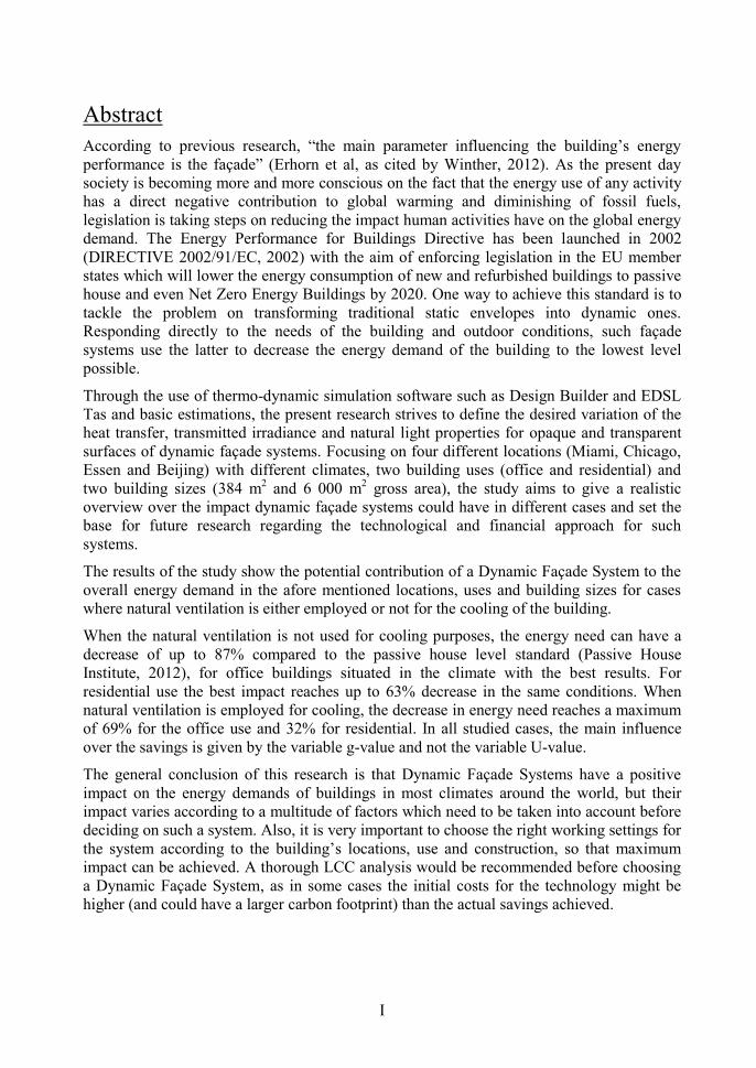
Abstract According to previous research, “the main parameter influencing the building’s energy performance is the façade” (Erhorn et al, as cited by Winther, 2012). As the present day society is becoming more and more conscious on the fact that the energy use of any activity has a direct negative contribution to global warming and diminishing of fossil fuels, legislation is taking steps on reducing the impact human activities have on the global energy demand. The Energy Performance for Buildings Directive has been launched in 2002 (DIRECTIVE 2002/91/EC, 2002) with the aim of enforcing legislation in the EU member states which will lower the energy consumption of new and refurbished buildings to passive house and even Net Zero Energy Buildings by 2020. One way to achieve this standard is to tackle the problem on transforming traditional static envelopes into dynamic ones. Responding directly to the needs of the building and outdoor conditions, such façade systems use the latter to decrease the energy demand of the building to the lowest level possible.
Through the use of thermo-dynamic simulation software such as Design Builder and EDSL Tas and basic estimations, the present research strives to define the desired variation of the heat transfer, transmitted irradiance and natural light properties for opaque and transparent surfaces of dynamic façade systems. Focusing on four different locations (Miami, Chicago, Essen and Beijing) with different climates, two building uses (office and residential) and two building sizes (384 m2 and 6 000 m2 gross area), the study aims to give a realistic overview over the impact dynamic façade systems could have in different cases and set the base for future research regarding the technological and financial approach for such systems.
The results of the study show the potential contribution of a Dynamic Façade System to the overall energy demand in the afore mentioned locations, uses and building sizes for cases where natural ventilation is either employed or not for the cooling of the building.
When the natural ventilation is not used for cooling purposes, the energy need can have a decrease of up to 87% compared to the passive house level standard (Passive House Institute, 2012), for office buildings situated in the climate with the best results. For residential use the best impact reaches up to 63% decrease in the same conditions. When natural ventilation is employed for cooling, the decrease in energy need reaches a maximum of 69% for the office use and 32% for residential. In all studied cases, the main influence over the savings is given by the variable g-value and not the variable U-value.
The general conclusion of this research is that Dynamic Façade Systems have a positive impact on the energy demands of buildings in most climates around the world, but their impact varies according to a multitude of factors which need to be taken into account before deciding on such a system. Also, it is very important to choose the right working settings for the system according to the building’s locations, use and construction, so that maximum impact can be achieved. A thorough LCC analysis would be recommended before choosing a Dynamic Façade System, as in some cases the initial costs for the technology might be higher (and could have a larger carbon footprint) than the actual savings achieved.
2
Preface The present document represents the final project of the master degree, promotion 2014, in the field of Energy-efficient and Environmental Building Design from Lund University.
The thesis has been developed in collaboration with LUWOGE consult GmbH and BASF Germany as a research project in the field of Dynamic Façade Systems. The project has been supervised by assistant prof. Åke Blomsterberg, senior researcher in the department of Energy and Building Design, Architecture and Built Environment of Lund University, Sweden and dipl. ing. arch. Thilo Cunz, senior manager at LUWOGE consult GmbH, Germany.
The thesis strives to give a not-too-complicated account of a rather complicated undertaking on the potential impact of dynamic façade systems. References to literature are made using the Harvard Referencing System, which shows references in brackets as follows: “quotation” (author, published year).
I found this project to be quite a challenge for the three months and 28 days I had for it and I am quite sure I could not have reached the end in due time without the help of some very friendly, supportive and dedicated people, that put up with my complaints about learning how to use Tas and lack of sleep. My special thanks goes to: Åke Blomsterberg- for the great feedback, constant encouragements and for bearing with me and my hectic schedule, Thilo Cunz- for believing in a Romanian girl, from a Swedish University, that he never met in person and never heard of before, Andreas Kirbach- my mentor, shoulder-to-cry-on, company in the lunch-breaks and German (+Tas) teacher, Nikolaus Nestle, Ralf Nörenberg and Jens Carsten Röder- for choosing to read an e-mail from a perfect stranger and to give that stranger a chance to prove herself and support her in the process, Henrik Davidsson- for encouraging me throughout my training and showing me what good teaching is all about, Kaisa Svenberg- for taking the time to introduce us to the world of “Master Thesis” and supporting us in the process, Moritz Diesner and Timo Jäger- for their knowledgeable support and patience, Heike Haracska- for the moral support, nourishment and smiles, Felix Wohlfarth-who showed me how to use the much-needed coffee machine, Sabine Kielhorn-Bayer- for answering an e-mail sent to the contact address of BASF and not only forwarding it to the right people, but also giving me their contacts and last but not least, to Maria Wall, without whom I would have not had the chance to have this amazing experience to begin with and the Eliasson Foundation, who supported my studies in the past two years.
This covers the academic part of my thanks, and now I turn to my family and friends, to which I am most grateful for the amazing support they offered me in every time of need. I am extremely proud and thankful for the luck of having one of the greatest families anyone could wish for, and some of the most amazing friends one could imagine. A big-big “thank you!” to all of you, in whatever part of the world you are now!
Sinziana Rasca
June 2014

3
Terminology Scientific Terminology [is] the Scylla's cave which men of science are preparing for themselves to be able to pounce out upon us from it, and into which we cannot penetrate.
(Butler ,1917)
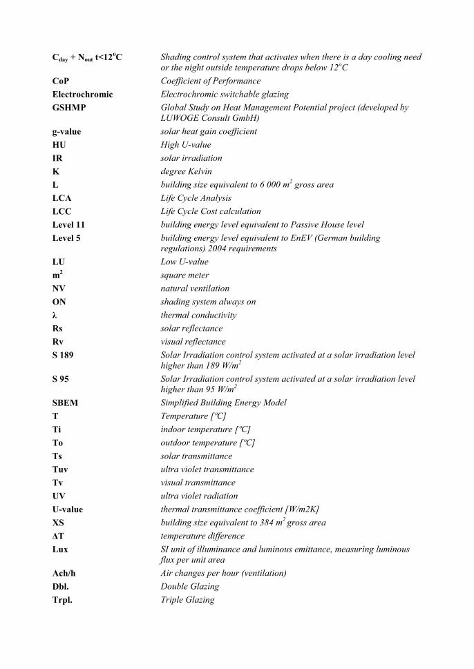
Cday + Nout t<12oC Shading control system that activates when there is a day cooling need or the night outside temperature drops below 12oC
CoP Coefficient of Performance Electrochromic Electrochromic switchable glazing GSHMP Global Study on Heat Management Potential project (developed by
LUWOGE Consult GmbH) g-value solar heat gain coefficient HU High U-value IR solar irradiation K degree Kelvin L building size equivalent to 6 000 m2 gross area LCA Life Cycle Analysis LCC Life Cycle Cost calculation Level 11 building energy level equivalent to Passive House level Level 5 building energy level equivalent to EnEV (German building
regulations) 2004 requirements LU Low U-value m2 square meter NV natural ventilation ON shading system always on λ thermal conductivity Rs solar reflectance Rv visual reflectance S 189 Solar Irradiation control system activated at a solar irradiation level
higher than 189 W/m2 S 95 Solar Irradiation control system activated at a solar irradiation level
higher than 95 W/m2 SBEM Simplified Building Energy Model T Temperature [ºC] Ti indoor temperature [ºC] To outdoor temperature [ºC] Ts solar transmittance Tuv ultra violet transmittance Tv visual transmittance UV ultra violet radiation U-value thermal transmittance coefficient [W/m2K] XS building size equivalent to 384 m2 gross area ΔT temperature difference Lux SI unit of illuminance and luminous emittance, measuring luminous
flux per unit area Ach/h Air changes per hour (ventilation) Dbl. Double Glazing Trpl. Triple Glazing

5
Clr. Clear Glass Low E Low Emissivity Glass WD Week Day WE Weekend Day
6
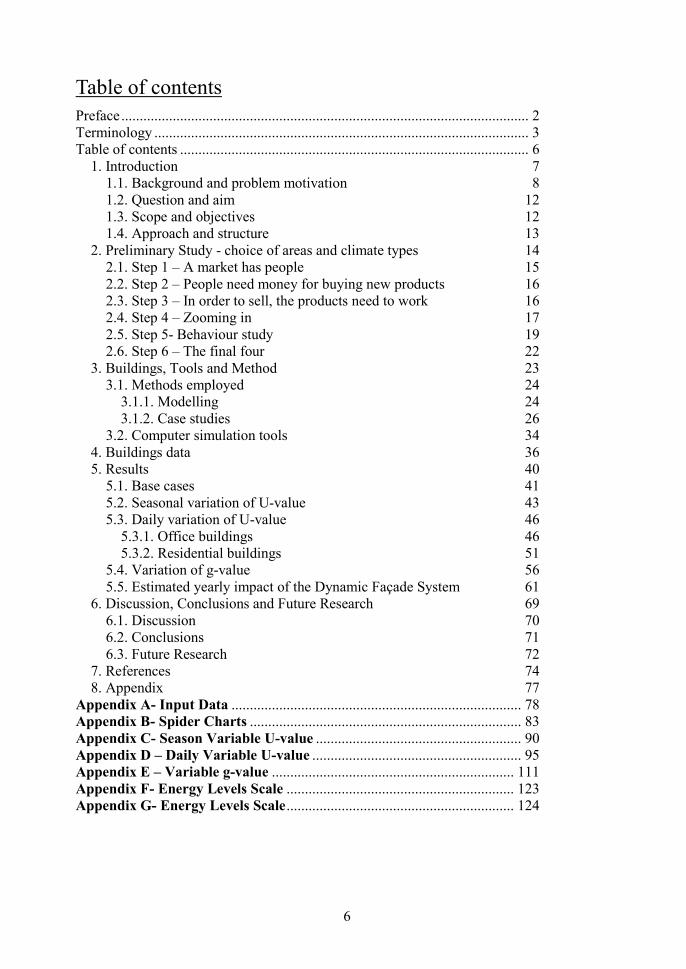
Table of contents Preface ............................................................................................................... 2 Terminology ...................................................................................................... 3 Table of contents ............................................................................................... 6
Introduction 7 1. Background and problem motivation 8 1.1. Question and aim 12 1.2. Scope and objectives 12 1.3. Approach and structure 13 1.4.
Preliminary Study - choice of areas and climate types 14 2. Step 1 – A market has people 15 2.1. Step 2 – People need money for buying new products 16 2.2. Step 3 – In order to sell, the products need to work 16 2.3. Step 4 – Zooming in 17 2.4. Step 5- Behaviour study 19 2.5. Step 6 – The final four 22 2.6.
Buildings, Tools and Method 23 3. Methods employed 24 3.1.
3.1.1. Modelling 24 3.1.2. Case studies 26 Computer simulation tools 34 3.2.
Buildings data 36 4. Results 40 5.
Base cases 41 5.1. Seasonal variation of U-value 43 5.2. Daily variation of U-value 46 5.3.
5.3.1. Office buildings 46 5.3.2. Residential buildings 51 Variation of g-value 56 5.4. Estimated yearly impact of the Dynamic Façade System 61 5.5.
Discussion, Conclusions and Future Research 69 6. Discussion 70 6.1. Conclusions 71 6.2. Future Research 72 6.3.
References 74 7. Appendix 77 8.
Appendix A- Input Data ............................................................................... 78 Appendix B- Spider Charts .......................................................................... 83 Appendix C- Season Variable U-value ........................................................ 90 Appendix D – Daily Variable U-value ......................................................... 95 Appendix E – Variable g-value .................................................................. 111 Appendix F- Energy Levels Scale .............................................................. 123 Appendix G- Energy Levels Scale .............................................................. 124
Dynamic Facade Systems- Master Thesis, LTH Sînziana Râșca
7
Introduction 1.
The main parameter influencing the building’s energy-performance is the façade.
(Erhorn et al, as cited in Winther, 2012)
Dynamic Facade Systems- Master Thesis, LTH Sînziana Râșca
8
Background and problem motivation 1.1.
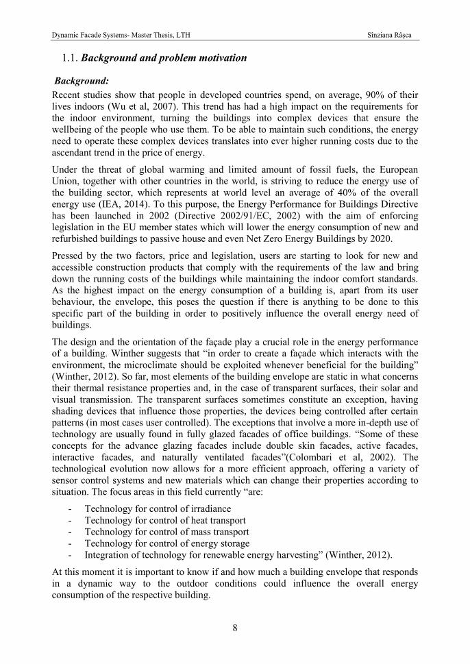
Background: Recent studies show that people in developed countries spend, on average, 90% of their lives indoors (Wu et al, 2007). This trend has had a high impact on the requirements for the indoor environment, turning the buildings into complex devices that ensure the wellbeing of the people who use them. To be able to maintain such conditions, the energy need to operate these complex devices translates into ever higher running costs due to the ascendant trend in the price of energy.
Under the threat of global warming and limited amount of fossil fuels, the European Union, together with other countries in the world, is striving to reduce the energy use of the building sector, which represents at world level an average of 40% of the overall energy use (IEA, 2014). To this purpose, the Energy Performance for Buildings Directive has been launched in 2002 (Directive 2002/91/EC, 2002) with the aim of enforcing legislation in the EU member states which will lower the energy consumption of new and refurbished buildings to passive house and even Net Zero Energy Buildings by 2020.
Pressed by the two factors, price and legislation, users are starting to look for new and accessible construction products that comply with the requirements of the law and bring down the running costs of the buildings while maintaining the indoor comfort standards. As the highest impact on the energy consumption of a building is, apart from its user behaviour, the envelope, this poses the question if there is anything to be done to this specific part of the building in order to positively influence the overall energy need of buildings.
The design and the orientation of the façade play a crucial role in the energy performance of a building. Winther suggests that “in order to create a façade which interacts with the environment, the microclimate should be exploited whenever beneficial for the building” (Winther, 2012). So far, most elements of the building envelope are static in what concerns their thermal resistance properties and, in the case of transparent surfaces, their solar and visual transmission. The transparent surfaces sometimes constitute an exception, having shading devices that influence those properties, the devices being controlled after certain patterns (in most cases user controlled). The exceptions that involve a more in-depth use of technology are usually found in fully glazed facades of office buildings. “Some of these concepts for the advance glazing facades include double skin facades, active facades, interactive facades, and naturally ventilated facades”(Colombari et al, 2002). The technological evolution now allows for a more efficient approach, offering a variety of sensor control systems and new materials which can change their properties according to situation. The focus areas in this field currently “are:
- Technology for control of irradiance - Technology for control of heat transport - Technology for control of mass transport - Technology for control of energy storage - Integration of technology for renewable energy harvesting” (Winther, 2012).
At this moment it is important to know if and how much a building envelope that responds in a dynamic way to the outdoor conditions could influence the overall energy consumption of the respective building.
Dynamic Facade Systems- Master Thesis, LTH Sînziana Râșca
9
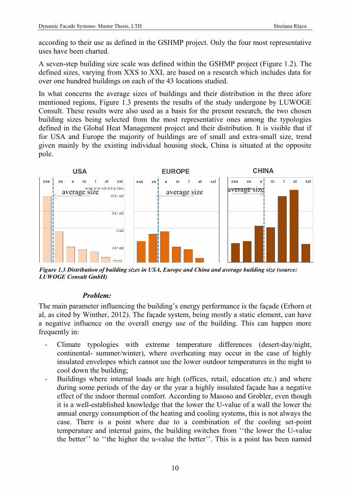
Figure 1.2 Building Sizes for Offices (LUWOGE Consult GmbH)
XXS XS S M
L
XL
XXL
The world of science is already looking into the possibilities, research projects such as the PhD thesis of F.V. Winther, “Intelligent Glazed Facades- An experimental study”, focusing on the subject of dynamic properties of glazed façade elements. There are currently no published articles on the overall impact that a fully dynamic envelope (where both the opaque surfaces and the transparent ones have dynamic thermal resistances and solar transmittances- the latter only for transparent areas) would have on a building’s energy consumption.
The present study, developed with the support of the specialists at LUWOGE consult GmbH, Germany, strives to give an estimate on how a dynamic façade system would influence the building energy need and thus provide the base for future analysis of potential markets for such products. Based on several research projects previously undertaken by the company, the study will refer throughout its length to those projects where relevant.
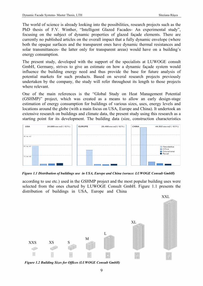
One of the main references is the “Global Study on Heat Management Potential (GSHMP)” project, which was created as a means to allow an early design-stage estimation of energy consumption for buildings of various sizes, uses, energy levels and locations around the globe (with a main focus on USA, Europe and China). It undertook an extensive research on buildings and climate data, the present study using this research as a starting point for its development. The building data (size, construction characteristics
according to use etc.) used in the GSHMP project and the most popular building uses were selected from the ones charted by LUWOGE Consult GmbH. Figure 1.1 presents the distribution of buildings in USA, Europe and China
Figure 1.1 Distribution of buildings use in USA, Europe and China (soruce: LUWOGE Consult GmbH)
Dynamic Facade Systems- Master Thesis, LTH Sînziana Râșca
10
according to their use as defined in the GSHMP project. Only the four most representative uses have been charted.
A seven-step building size scale was defined within the GSHMP project (Figure 1.2). The defined sizes, varying from XXS to XXL are based on a research which includes data for over one hundred buildings on each of the 43 locations studied.
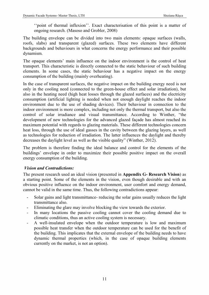
In what concerns the average sizes of buildings and their distribution in the three afore mentioned regions, Figure 1.3 presents the results of the study undergone by LUWOGE Consult. These results were also used as a basis for the present research, the two chosen building sizes being selected from the most representative ones among the typologies defined in the Global Heat Management project and their distribution. It is visible that if for USA and Europe the majority of buildings are of small and extra-small size, trend given mainly by the existing individual housing stock, China is situated at the opposite pole.
Problem: The main parameter influencing the building’s energy performance is the façade (Erhorn et al, as cited by Winther, 2012). The façade system, being mostly a static element, can have a negative influence on the overall energy use of the building. This can happen more frequently in:
- Climate typologies with extreme temperature differences (desert-day/night, continental- summer/winter), where overheating may occur in the case of highly insulated envelopes which cannot use the lower outdoor temperatures in the night to cool down the building;
- Buildings where internal loads are high (offices, retail, education etc.) and where during some periods of the day or the year a highly insulated façade has a negative effect of the indoor thermal comfort. According to Masoso and Grobler, even though it is a well-established knowledge that the lower the U-value of a wall the lower the annual energy consumption of the heating and cooling systems, this is not always the case. There is a point where due to a combination of the cooling set-point temperature and internal gains, the building switches from ‘‘the lower the U-value the better’’ to ‘‘the higher the u-value the better’’. This is a point has been named
Figure 1.3 Distribution of building sizes in USA, Europe and China and average building size (source: LUWOGE Consult GmbH)
average size average size average size
Dynamic Facade Systems- Master Thesis, LTH Sînziana Râșca
11
‘‘point of thermal inflexion’’. Exact characterisation of this point is a matter of ongoing research. (Masoso and Grobler, 2008)
The building envelope can be divided into two main elements: opaque surfaces (walls, roofs, slabs) and transparent (glazed) surfaces. These two elements have different backgrounds and behaviours in what concerns the energy performance and their possible dynamism.
The opaque elements’ main influence on the indoor environment is the control of heat transport. This characteristic is directly connected to the static behaviour of such building elements. In some cases, the static behaviour has a negative impact on the energy consumption of the building (mainly overheating).
In the case of transparent surfaces, the negative impact on the building energy need is not only in the cooling need (connected to the green-house effect and solar irradiation), but also in the heating need (high heat losses through the glazed surfaces) and the electricity consumption (artificial lighting is needed when not enough daylight reaches the indoor environment due to the use of shading devices). Their behaviour in connection to the indoor environment is more complex, including not only the thermal transport, but also the control of solar irradiance and visual transmittance. According to Winther, “the development of new technologies for the advanced glazed façade has almost reached its maximum potential with regards to glazing materials. These different technologies concern heat loss, through the use of ideal gasses in the cavity between the glazing layers, as well as technologies for reduction of irradiation. The latter influences the daylight and thereby decreases the daylight level as well as the visible quality” (Winther, 2012).
The problem is therefore finding the ideal balance and control for the elements of the buildings’ envelope in order to maximize their possible positive impact on the overall energy consumption of the building.
Vision and Contradictions: The present research used an ideal vision (presented in Appendix G- Research Vision) as a starting point. Some of the elements in the vision, even though desirable and with an obvious positive influence on the indoor environment, user comfort and energy demand, cannot be valid in the same time. Thus, the following contradictions appear:
- Solar gains and light transmittance- reducing the solar gains usually reduces the light transmittance also.
- Eliminating the glare may involve blocking the view towards the exterior. - In many locations the passive cooling cannot cover the cooling demand due to
climatic conditions, thus an active cooling system is necessary. - A well-insulated envelope when the outdoor temperature is low and maximum
possible heat transfer when the outdoor temperature can be used for the benefit of the building. This implicates that the external envelope of the building needs to have dynamic thermal properties (which, in the case of opaque building elements currently on the market, is not an option).
Dynamic Facade Systems- Master Thesis, LTH Sînziana Râșca
12
Question and aim 1.2.
Question to be answered If we had dynamic construction elements for the external envelope of buildings, which system properties should they have for walls (U-value) and windows (U-value and g-value) compared to the passive house level, according to building use, size and construction, under different climatic conditions, in order to positively influence the overall energy demand of the building?
Aim The main aim of this study is to determine the system properties needed for dynamic façade elements that could be applicable for different building uses, different sizes in specific climates so that the best possible energy efficiency level is met. There are two reference levels considered: the passive house level energy consumption (defined as Level 11 in the “Global Study on Heat Management Potential (GSHMP)” project developed by Luwoge Consult GmbH, 2011) and year 2004 German energy certification level consumption (EnEV, 2004), defined as Level 5 in the same project.
Scope and objectives 1.3.
Scope The scope of the study is to test the possible performance of Dynamic Façade Systems for two building typologies (XS- size, 384 m2 and L-size 6 000 m2 gross area) and two different uses (residential and offices) in four different micro-climates (climate codes 4.55.2, 6.25.2, 6.24.3 and 6.34.4- as presented in Figure 2.4) which host highly populated areas from countries with a GDP per capita higher than the world average of 10 700 USD (MECOmeter, 2012). The testing will be done for four cities situated within the chosen micro-climates (Miami, Chicago, Essen and Beijing).
Limitations and assumptions Several limitations and assumptions were made in order to be able to perform the study in the given time-frame of four months. These can be found stated below:
- Two building uses: residential, office; - Two building sizes: XS- 384 m2, L- 6 000 m2, as presented in Figure 1.2; - Two building ages: new buildings (main focus), buildings constructed around 2004; - Two energy standards: new buildings, Level 11 – passive house standard (Passive
House Institute, 2012) and Level 5- equivalent for 2004 energy level in constructions as defined by German law (EnEV, 2004);
- Four locations: Miami, Chicago, Essen, Beijing; - Three climate types, according to Kopplen-Geiger classification (Kopen-Geiger
VU-Wien, 2011) (see Section 2.3 of the present study for details on the choice made): tropical monsoon – Miami, temperate oceanic- Essen and humid continental- Chicago and Beijing;
- Four microclimates, as defined by Luwoge consult GmbH (Figure 2.4): Miami- 4.55.2 , Beijing- 6.25.2, Chicago- 6.24.3 , Essen- 6.34.4.
The settings in Appendix A- Input Data will be used in all simulations; - Price per kWh: heating – 0.08 €, electricity – 0.137 € (Eurostat, 2013);
Dynamic Facade Systems- Master Thesis, LTH Sînziana Râșca
13
- The buildings will be modelled as simple parallelepipeds, with the long facades oriented on the North-South direction;
- Inner walls will be defined only on the L-size building, and kept to a minimum in order to reduce simulation time;
- No research will be done on the technical aspects of the facade system itself; - No interior features other than thermal comfort of the occupants and air quality
requirements will be considered.
Objectives The study has three major objectives defined: O1. Establish the variation range for the U-value of the walls
O2. Establish the recommended shading system (shading device and optimal control for it) for the windows.
O2. Establish the possible contribution of the Dynamic Façade System to the overall energy demand of the studied buildings in each studied climate.
Approach and structure 1.4. The present study tackles an innovative subject in the field of building envelopes. Due to the novelty of such technologies, and the future prospects of the studied product, the approach has been customized to fit the possible simulations with existing software and present, in an easy to understand way, the achieved results. The following section summarizes the course of action taken in the research and gives an overview of the preliminary study undertaken.
Course of action The course of action taken in the study has been divided in three main parts: Preliminary study, Computer simulations and Final Conclusions. Listed below is a short description of the undertaken steps in each part.
- Preliminary study o Motivate the choice of the final four locations to be analysed in the rest of
the study. - Computer simulations
o Collect data (sizes, U-values, heat-recovery system efficiency etc.) from the GSHMP simulation tool (described in section 3.2 of this report) for each studied building in all considered climates, for Level 11 and Level 5 (all input information can be found in Appendix A);
o Perform simulations for each case considered in the study and collect data for further analysis;
o Analyse the daily temperature for each location to determine the potential days in which the Dynamic Façade System could be used and estimate the decrease in the yearly energy demand compared to the passive house level;
o Analyse and present the results both for each particular case but also in comparison to each other.
- Final Conclusions o Draw the final conclusions of the research;
o Highlight the possibilities of future research in the field.
Dynamic Facade Systems- Master Thesis, LTH Sînziana Râșca
14
Preliminary Study - choice of areas and climate types 2.
A study of the history of opinion is a necessary preliminary to the emancipation of the mind.
(John Maynard Keynes)
Dynamic Facade Systems- Master Thesis, LTH Sînziana Râșca
15
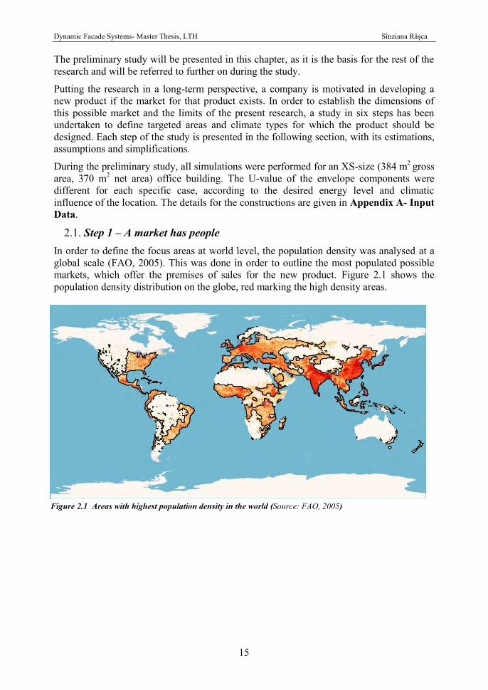
Figure 2.1 Areas with highest population density in the world (Source: FAO, 2005)
The preliminary study will be presented in this chapter, as it is the basis for the rest of the research and will be referred to further on during the study.
Putting the research in a long-term perspective, a company is motivated in developing a new product if the market for that product exists. In order to establish the dimensions of this possible market and the limits of the present research, a study in six steps has been undertaken to define targeted areas and climate types for which the product should be designed. Each step of the study is presented in the following section, with its estimations, assumptions and simplifications.
During the preliminary study, all simulations were performed for an XS-size (384 m2 gross area, 370 m2 net area) office building. The U-value of the envelope components were different for each specific case, according to the desired energy level and climatic influence of the location. The details for the constructions are given in Appendix A- Input Data.
Step 1 – A market has people 2.1. In order to define the focus areas at world level, the population density was analysed at a global scale (FAO, 2005). This was done in order to outline the most populated possible markets, which offer the premises of sales for the new product. Figure 2.1 shows the population density distribution on the globe, red marking the high density areas.
Dynamic Facade Systems- Master Thesis, LTH Sînziana Râșca
16
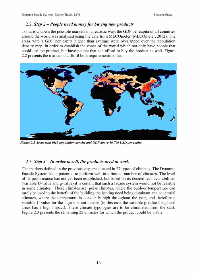
Step 2 – People need money for buying new products 2.2. To narrow down the possible markets in a realistic way, the GDP per capita of all countries around the world was analysed using the data from MECOmeter (MECOmeter, 2012). The areas with a GDP per capita higher than average were overlapped over the population density map, in order to establish the zones of the world which not only have people that could use the product, but have people that can afford to buy the product as well. Figure 2.2 presents the markets that fulfil both requirements so far.
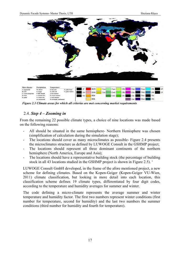
Step 3 – In order to sell, the products need to work 2.3. The markets defined in the previous step are situated in 27 types of climates. The Dynamic Façade System has a potential to perform well in a limited number of climates. The level of its performance has not yet been established, but based on its desired technical abilities (variable U-value and g-value) it is certain that such a façade system would not be feasible in some climates. These climates are: polar climates, where the outdoor temperature can rarely be used to the benefit of the building the heating need being dominant and equatorial climates, where the temperature is constantly high throughout the year, and therefore a variable U-value for the façade is not needed (in this case the variable g-value for glazed areas has a high impact). These climate typologies are to be eliminated from the start. Figure 2.3 presents the remaining 22 climates for which the product could be viable.
Figure 2.2 Areas with high population density and GDP above 10 700 USD per capita
Dynamic Facade Systems- Master Thesis, LTH Sînziana Râșca
17
Step 4 – Zooming in 2.4. From the remaining 22 possible climate types, a choice of nine locations was made based on the following reasons:
- All should be situated in the same hemisphere- Northern Hemisphere was chosen (simplification of calculation during the simulation stage);
- The locations should cover as many microclimates as possible- Figure 2.4 presents the microclimates structure as defined by LUWOGE Consult in the GSHMP project;
- The locations should represent all three dominant continents of the northern hemisphere (North America, Europe and Asia);
- The locations should have a representative building stock (the percentage of building stock in all 43 locations studied in the GSHMP project is shown in Figure 2.5). ‘
LUWOGE Consult GmbH developed, in the frame of the afore mentioned project, a new scheme for defining climates. Based on the Kopen-Geiger (Kopen-Geiger VU-Wien, 2011) climate classification, but looking in more detail into each location, this classification scheme defines 19 climate types, differentiated by four digit codes, according to the temperature and humidity averages for summer and winter.
The code defining a micro-climate represents the average summer and winter temperature and humidity factor. The first two numbers represent winter conditions (first number for temperature, second for humidity) and the last two numbers the summer conditions (third number for humidity and fourth for temperature).
Figure 2.3 Climate areas for which all criterias are met concerning market requirements
Dynamic Facade Systems- Master Thesis, LTH Sînziana Râșca
18
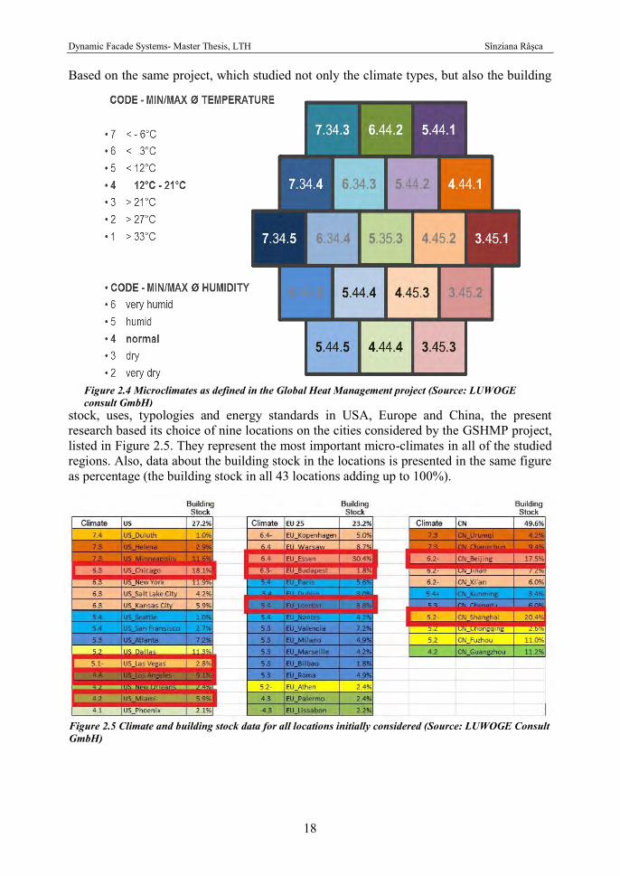
Figure 2.4 Microclimates as defined in the Global Heat Management project (Source: LUWOGE consult GmbH)
Based on the same project, which studied not only the climate types, but also the building
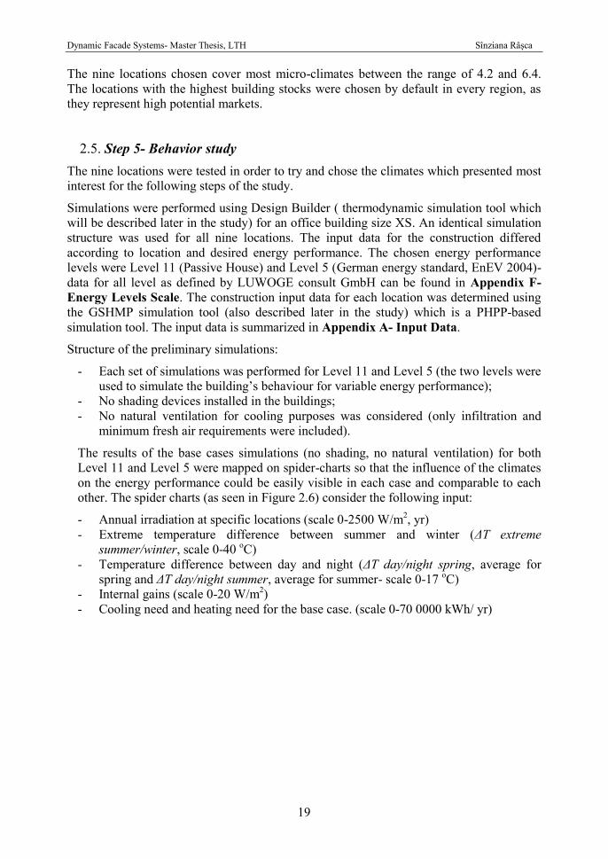
stock, uses, typologies and energy standards in USA, Europe and China, the present research based its choice of nine locations on the cities considered by the GSHMP project, listed in Figure 2.5. They represent the most important micro-climates in all of the studied regions. Also, data about the building stock in the locations is presented in the same figure as percentage (the building stock in all 43 locations adding up to 100%).
Figure 2.5 Climate and building stock data for all locations initially considered (Source: LUWOGE Consult GmbH)
Dynamic Facade Systems- Master Thesis, LTH Sînziana Râșca
19
The nine locations chosen cover most micro-climates between the range of 4.2 and 6.4. The locations with the highest building stocks were chosen by default in every region, as they represent high potential markets.
Step 5- Behavior study 2.5. The nine locations were tested in order to try and chose the climates which presented most interest for the following steps of the study.
Simulations were performed using Design Builder ( thermodynamic simulation tool which will be described later in the study) for an office building size XS. An identical simulation structure was used for all nine locations. The input data for the construction differed according to location and desired energy performance. The chosen energy performance levels were Level 11 (Passive House) and Level 5 (German energy standard, EnEV 2004)- data for all level as defined by LUWOGE consult GmbH can be found in Appendix F- Energy Levels Scale. The construction input data for each location was determined using the GSHMP simulation tool (also described later in the study) which is a PHPP-based simulation tool. The input data is summarized in Appendix A- Input Data.
Structure of the preliminary simulations:
- Each set of simulations was performed for Level 11 and Level 5 (the two levels were used to simulate the building’s behaviour for variable energy performance);
- No shading devices installed in the buildings; - No natural ventilation for cooling purposes was considered (only infiltration and
minimum fresh air requirements were included).
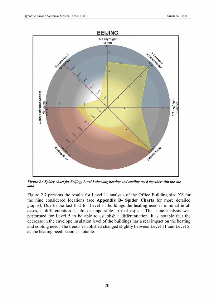
The results of the base cases simulations (no shading, no natural ventilation) for both Level 11 and Level 5 were mapped on spider-charts so that the influence of the climates on the energy performance could be easily visible in each case and comparable to each other. The spider charts (as seen in Figure 2.6) consider the following input:
- Annual irradiation at specific locations (scale 0-2500 W/m2, yr) - Extreme temperature difference between summer and winter (ΔT extreme
summer/winter, scale 0-40 oC) - Temperature difference between day and night (ΔT day/night spring, average for
spring and ΔT day/night summer, average for summer- scale 0-17 oC) - Internal gains (scale 0-20 W/m2) - Cooling need and heating need for the base case. (scale 0-70 0000 kWh/ yr)
Dynamic Facade Systems- Master Thesis, LTH Sînziana Râșca
20
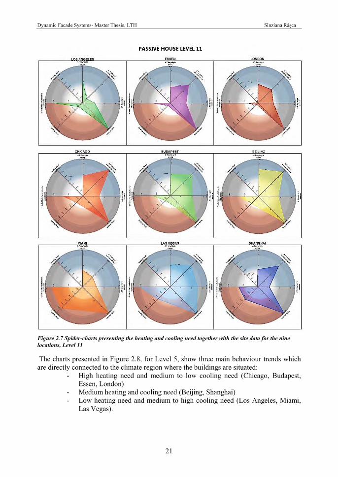
Figure 2.7 presents the results for Level 11 analysis of the Office Building size XS for the nine considered locations (see Appendix B- Spider Charts for more detailed graphs). Due to the fact that for Level 11 buildings the heating need is minimal in all cases, a differentiation is almost impossible in that aspect. The same analysis was performed for Level 5 to be able to establish a differentiation. It is notable that the decrease in the envelope insulation level of the buildings has a real impact on the heating and cooling need. The trends established changed slightly between Level 11 and Level 5, as the heating need becomes notable.
Figure 2.6 Spider-chart for Beijing, Level 5 showing heating and cooling need together with the site-data
Dynamic Facade Systems- Master Thesis, LTH Sînziana Râșca
21
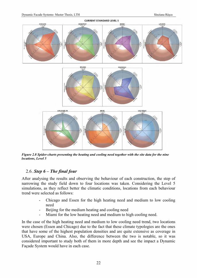
The charts presented in Figure 2.8, for Level 5, show three main behaviour trends which are directly connected to the climate region where the buildings are situated:
- High heating need and medium to low cooling need (Chicago, Budapest, Essen, London)
- Medium heating and cooling need (Beijing, Shanghai) - Low heating need and medium to high cooling need (Los Angeles, Miami,
Las Vegas).
Figure 2.7 Spider-charts presenting the heating and cooling need together with the site data for the nine locations, Level 11
Dynamic Facade Systems- Master Thesis, LTH Sînziana Râșca
22
Figure 2.8 Spider-charts presenting the heating and cooling need together with the site data for the nine locations, Level 5
Step 6 – The final four 2.6. After analysing the results and observing the behaviour of each construction, the step of narrowing the study field down to four locations was taken. Considering the Level 5 simulations, as they reflect better the climatic conditions, locations from each behaviour trend were selected as follows:
- Chicago and Essen for the high heating need and medium to low cooling need
- Beijing for the medium heating and cooling need - Miami for the low heating need and medium to high cooling need.
In the case of the high heating need and medium to low cooling need trend, two locations were chosen (Essen and Chicago) due to the fact that these climate typologies are the ones that have some of the highest population densities and are quite extensive as coverage in USA, Europe and China. Also, the difference between the two is notable, so it was considered important to study both of them in more depth and see the impact a Dynamic Façade System would have in each case.

Dynamic Facade Systems- Master Thesis, LTH Sînziana Râșca
23
Methods and Tools 3.
By making the façade adaptable to changing weather conditions, less energy is needed for room heating and cooling compared with a façade that is unable to adapt.
(Jansen et al, 2003)
Dynamic Facade Systems- Master Thesis, LTH Sînziana Râșca
24
The following chapter presents the research performed in connection to the heat transfer, transmitted solar irradiation and light transfer properties of Dynamic Facade systems. It aims to describe the methods employed to reach the results concerning the potential impact of such systems on the overall energy demand of different building typologies in different climates and the tools chosen to perform simulations in different fields.
Methods employed 3.1.
3.1.1. Modelling For the two dynamic simulation tools, Design Builder and EDSL Tas, 3D models of the buildings had to be built and properties assigned to the building components and user profiles in order to perform realistic simulations.
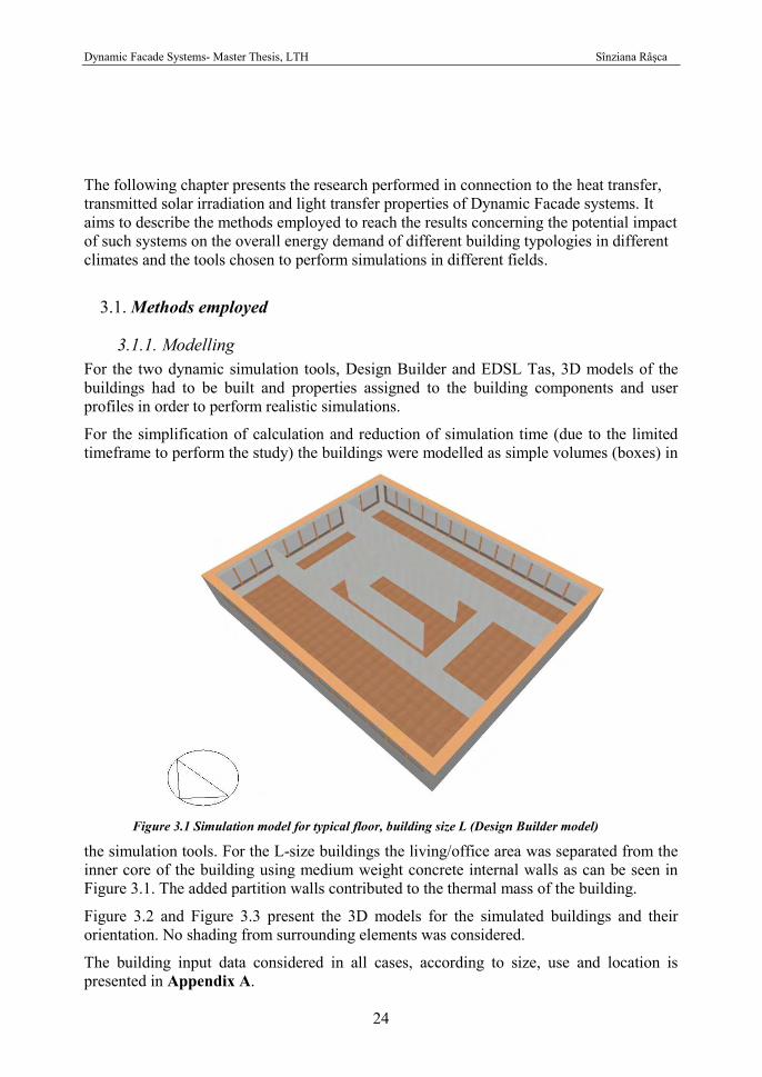
For the simplification of calculation and reduction of simulation time (due to the limited timeframe to perform the study) the buildings were modelled as simple volumes (boxes) in
the simulation tools. For the L-size buildings the living/office area was separated from the inner core of the building using medium weight concrete internal walls as can be seen in Figure 3.1. The added partition walls contributed to the thermal mass of the building.
Figure 3.2 and Figure 3.3 present the 3D models for the simulated buildings and their orientation. No shading from surrounding elements was considered.
The building input data considered in all cases, according to size, use and location is presented in Appendix A.
Figure 3.1 Simulation model for typical floor, building size L (Design Builder model)
Dynamic Facade Systems- Master Thesis, LTH Sînziana Râșca
25
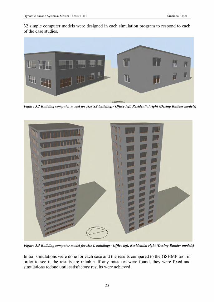
Figure 3.2 Building computer model for size XS buildings- Office left, Residential right (Desing Builder models)
Figure 3.3 Building computer model for size L buildings- Office left, Residential right (Desing Builder models)
32 simple computer models were designed in each simulation program to respond to each of the case studies.
Initial simulations were done for each case and the results compared to the GSHMP tool in order to see if the results are reliable. If any mistakes were found, they were fixed and simulations redone until satisfactory results were achieved.
Dynamic Facade Systems- Master Thesis, LTH Sînziana Râșca
26
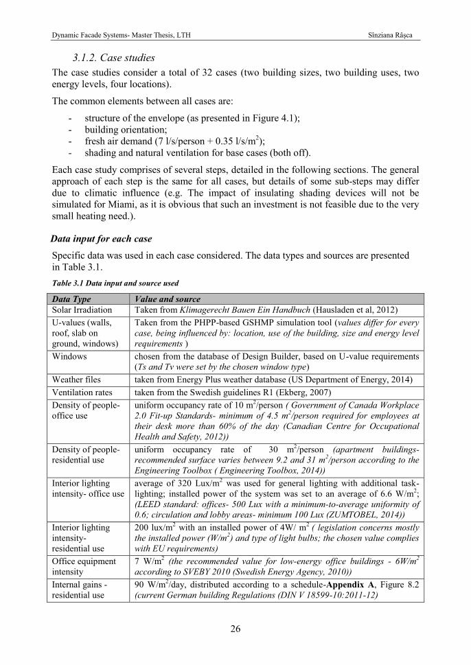
3.1.2. Case studies The case studies consider a total of 32 cases (two building sizes, two building uses, two energy levels, four locations).
The common elements between all cases are:
- structure of the envelope (as presented in Figure 4.1); - building orientation; - fresh air demand (7 l/s/person + 0.35 l/s/m2); - shading and natural ventilation for base cases (both off).
Each case study comprises of several steps, detailed in the following sections. The general approach of each step is the same for all cases, but details of some sub-steps may differ due to climatic influence (e.g. The impact of insulating shading devices will not be simulated for Miami, as it is obvious that such an investment is not feasible due to the very small heating need.).
Data input for each case
Specific data was used in each case considered. The data types and sources are presented in Table 3.1. Table 3.1 Data input and source used
Data Type Value and source Solar Irradiation Taken from Klimagerecht Bauen Ein Handbuch (Hausladen et al, 2012) U-values (walls, roof, slab on ground, windows)
Taken from the PHPP-based GSHMP simulation tool (values differ for every case, being influenced by: location, use of the building, size and energy level requirements )
Windows chosen from the database of Design Builder, based on U-value requirements (Ts and Tv were set by the chosen window type)
Weather files taken from Energy Plus weather database (US Department of Energy, 2014) Ventilation rates taken from the Swedish guidelines R1 (Ekberg, 2007) Density of people- office use
uniform occupancy rate of 10 m2/person ( Government of Canada Workplace 2.0 Fit-up Standards- minimum of 4.5 m2/person required for employees at their desk more than 60% of the day (Canadian Centre for Occupational Health and Safety, 2012))
Density of people- residential use
uniform occupancy rate of 30 m2/person (apartment buildings- recommended surface varies between 9.2 and 31 m2/person according to the Engineering Toolbox ( Engineering Toolbox, 2014))
Interior lighting intensity- office use
average of 320 Lux/m2 was used for general lighting with additional task-lighting; installed power of the system was set to an average of 6.6 W/m2; (LEED standard: offices- 500 Lux with a minimum-to-average uniformity of 0.6; circulation and lobby areas- minimum 100 Lux (ZUMTOBEL, 2014))
Interior lighting intensity- residential use
200 lux/m2 with an installed power of 4W/ m2 ( legislation concerns mostly the installed power (W/m2) and type of light bulbs; the chosen value complies with EU requirements)
Office equipment intensity
7 W/m2 (the recommended value for low-energy office buildings - 6W/m2 according to SVEBY 2010 (Swedish Energy Agency, 2010))
Internal gains - residential use
90 W/m2/day, distributed according to a schedule-Appendix A, Figure 8.2 (current German building Regulations (DIN V 18599-10:2011-12)
Dynamic Facade Systems- Master Thesis, LTH Sînziana Râșca
27
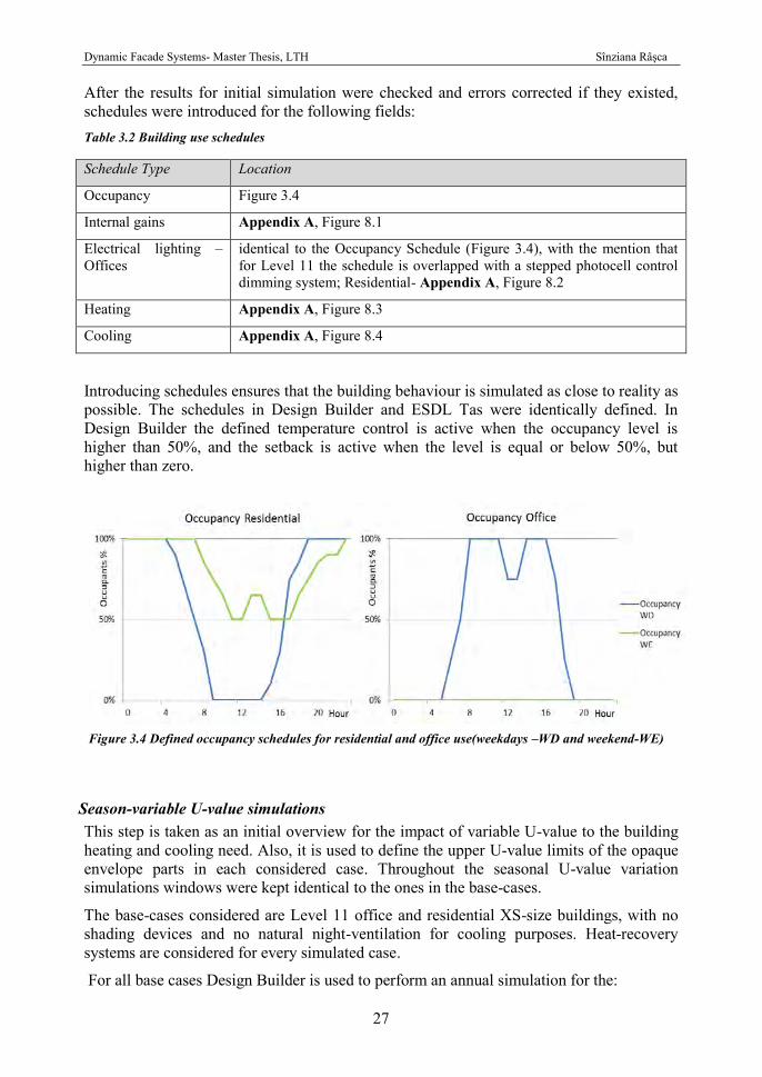
After the results for initial simulation were checked and errors corrected if they existed, schedules were introduced for the following fields: Table 3.2 Building use schedules
Schedule Type Location
Occupancy Figure 3.4
Internal gains Appendix A, Figure 8.1
Electrical lighting –Offices
identical to the Occupancy Schedule (Figure 3.4), with the mention that for Level 11 the schedule is overlapped with a stepped photocell control dimming system; Residential- Appendix A, Figure 8.2
Heating Appendix A, Figure 8.3
Cooling Appendix A, Figure 8.4
Introducing schedules ensures that the building behaviour is simulated as close to reality as possible. The schedules in Design Builder and ESDL Tas were identically defined. In Design Builder the defined temperature control is active when the occupancy level is higher than 50%, and the setback is active when the level is equal or below 50%, but higher than zero.
Season-variable U-value simulations This step is taken as an initial overview for the impact of variable U-value to the building heating and cooling need. Also, it is used to define the upper U-value limits of the opaque envelope parts in each considered case. Throughout the seasonal U-value variation simulations windows were kept identical to the ones in the base-cases.
The base-cases considered are Level 11 office and residential XS-size buildings, with no shading devices and no natural night-ventilation for cooling purposes. Heat-recovery systems are considered for every simulated case.
For all base cases Design Builder is used to perform an annual simulation for the:
Figure 3.4 Defined occupancy schedules for residential and office use(weekdays –WD and weekend-WE)
Dynamic Facade Systems- Master Thesis, LTH Sînziana Râșca
28
- Outdoor air temperature variation - Indoor dry bulb temperature variation - Solar gains through the windows - Heating need - Cooling need.
The output data is hourly, simulations being performed with one step per hour (limitation given by the weather files)1. In this way it is easy to see when the outdoor temperature and solar irradiation through the windows have an impact on the heating and cooling need.
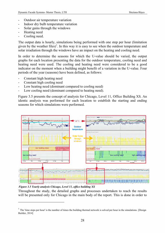
In order to determine the seasons for which the U-value should be varied, the output graphs for each location presenting the data for the outdoor temperature, cooling need and heating need were used. The cooling and heating need were considered to be a good indicator on the moment when a building might benefit of a variation in the U-value. Four periods of the year (seasons) have been defined, as follows:
- Constant high heating need - Constant high cooling need - Low heating need (dominant compared to cooling need) - Low cooling need (dominant compared to heating need).
Figure 3.5 presents the concept of analysis for Chicago, Level 11, Office Building XS. An identic analysis was performed for each location to establish the starting and ending seasons for which simulations were performed.
Throughout the study, the detailed graphs and processes undertaken to reach the results will be presented only for Chicago in the main body of the report. This is done in order to
1 The 'time steps per hour' is the number of times the building thermal network is solved per hour in the simulations. [Design Builder, 2014]
Figure 3.5 Yearly analysis Chicago, Level 11, office building XS
Outdoor temperature
Solar Gains through windows
Dynamic Facade Systems- Master Thesis, LTH Sînziana Râșca
29
limit the extent of the thesis. Chicago is used as a representative case, as its climate is met in a wide range of locations across USA, Europe and China and its features- hot summers, cold winters, notable day to night temperature differences, high level of solar irradiation- make it one of the best candidates for a Dynamic Façade System. For the rest of the locations, the detailed results are presented in the Appendix section.
Simulations are performed as a parametric study to see how the heating need and cooling need are affected in each case by the U-value variation. Insulation is decreased in steps, from the insulation level needed for the Passive House standard (Level 11) to the minimum level of 0 cm of insulation outside the concrete layer of the envelope (walls, roof, slab on ground). The windows were kept identical to the initial case throughout the simulations, as were the infiltration level, window shading, ventilation and all other corresponding settings.
To simplify the way to present the results, a “set” of insulating levels is defined for each location, each level being referred to afterwards with the thickness of the wall insulation. The corresponding U-values and insulation thicknesses can be consulted in Appendix C.
Daily-variable U-value simulations Varying the U-value of opaque and transparent surfaces of a building during 24 hours is not a task that the simulation programs used for the present study can perform. Due to this shortage in technology tools, a special approach had to be designed and an estimation as close to reality as possible attempted.
Transparent surfaces variable U-value Due to the time and technological constraints, this section of the research has not been detailed and its outcomes are not included in the final results.
External shading devices with insulating properties (Aerogel Silica), controlled by automatic control systems, were used to vary the U-value of the windows. Simulations are performed in Design Builder.
The results are not perfectly accurate, due to the lower limit of 5 cm imposed by the program for the air gap between the glazing and the shading device. This impacts the results negatively, due to the infiltration of outdoor air between the insulated shading and the window and the convective heat transfer which appears in the respective space. It is estimated that the results in reality are slightly better than the ones presented in this research.
The shading is activated by a temperature set automatic control. The shading is on when the night outdoor temperature falls below 12oC. This lower limit was chosen as a six degrees difference between the minimum accepted indoor temperature and the outdoor temperature. It is considered reasonable, anything below that probably influencing negatively the heating demand of the buildings.
Opaque surfaces variable U-value EDSL Tas simulation tool is used for simulating the U-value variation of opaque envelope areas. Due to the fact that Tas does not have an option for varying the U-value of building elements, the approach undertaken to study the building behaviour when the U-value varies is presented in steps in the following section.
Dynamic Facade Systems- Master Thesis, LTH Sînziana Râșca
30
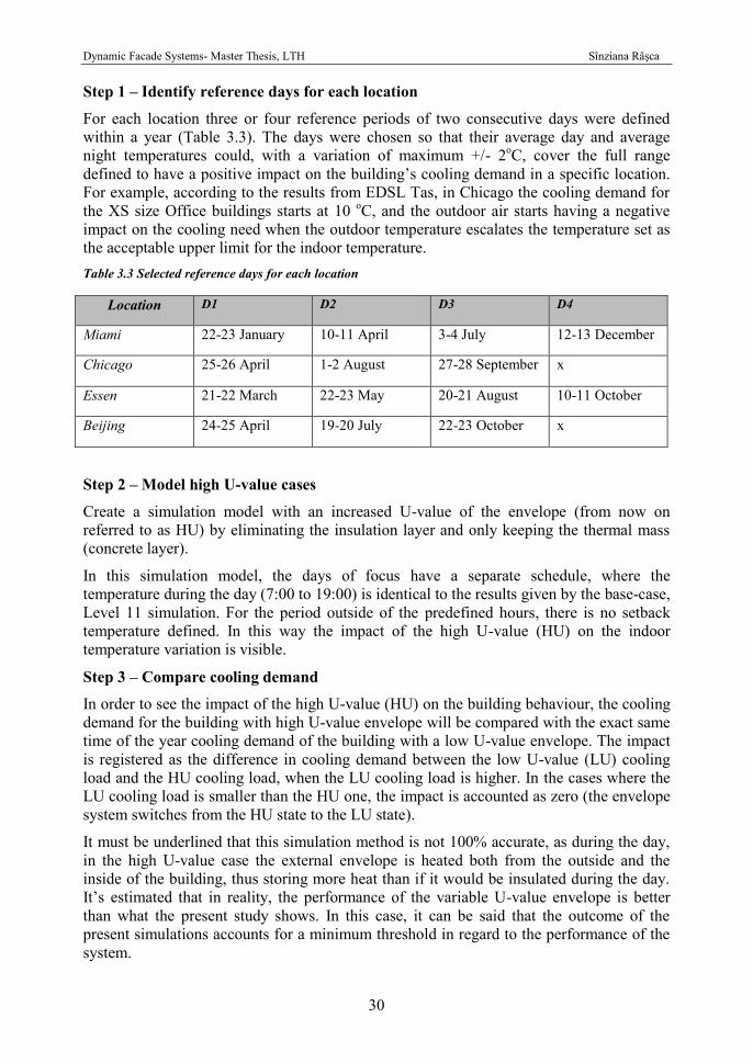
Step 1 – Identify reference days for each location
For each location three or four reference periods of two consecutive days were defined within a year (Table 3.3). The days were chosen so that their average day and average night temperatures could, with a variation of maximum +/- 2oC, cover the full range defined to have a positive impact on the building’s cooling demand in a specific location. For example, according to the results from EDSL Tas, in Chicago the cooling demand for the XS size Office buildings starts at 10 oC, and the outdoor air starts having a negative impact on the cooling need when the outdoor temperature escalates the temperature set as the acceptable upper limit for the indoor temperature. Table 3.3 Selected reference days for each location
Location D1 D2 D3 D4
Miami 22-23 January 10-11 April 3-4 July 12-13 December
Chicago 25-26 April 1-2 August 27-28 September x
Essen 21-22 March 22-23 May 20-21 August 10-11 October
Beijing 24-25 April 19-20 July 22-23 October x
Step 2 – Model high U-value cases
Create a simulation model with an increased U-value of the envelope (from now on referred to as HU) by eliminating the insulation layer and only keeping the thermal mass (concrete layer).
In this simulation model, the days of focus have a separate schedule, where the temperature during the day (7:00 to 19:00) is identical to the results given by the base-case, Level 11 simulation. For the period outside of the predefined hours, there is no setback temperature defined. In this way the impact of the high U-value (HU) on the indoor temperature variation is visible.
Step 3 – Compare cooling demand
In order to see the impact of the high U-value (HU) on the building behaviour, the cooling demand for the building with high U-value envelope will be compared with the exact same time of the year cooling demand of the building with a low U-value envelope. The impact is registered as the difference in cooling demand between the low U-value (LU) cooling load and the HU cooling load, when the LU cooling load is higher. In the cases where the LU cooling load is smaller than the HU one, the impact is accounted as zero (the envelope system switches from the HU state to the LU state).
It must be underlined that this simulation method is not 100% accurate, as during the day, in the high U-value case the external envelope is heated both from the outside and the inside of the building, thus storing more heat than if it would be insulated during the day. It’s estimated that in reality, the performance of the variable U-value envelope is better than what the present study shows. In this case, it can be said that the outcome of the present simulations accounts for a minimum threshold in regard to the performance of the system.
Dynamic Facade Systems- Master Thesis, LTH Sînziana Râșca
31
Step 4 – Estimate yearly savings
In order to estimate the yearly savings for each case, a special formula has been devised.
An outdoor day average temperature (06:00 to 21:00) and night average temperature (21:00 to 06:00) was calculated for the reference days in each location. These temperatures were compared to the day average and night average temperatures of every day in the year for each location. The days where the day or night average temperature was in a range of +/- 2oC to one of the reference days were counted separately. The final number of days of one specific type was defined as the average between the two resulting numbers.
For the estimation of the yearly savings, the savings for one specific reference day was multiplied with the number of days within a year with similar temperatures (counted in the previous step) and added to the savings from the other day typologies defined.
Variable g-value simulations The g-value or the total solar energy transmittance is defined as the direct transmittance through the glazing system plus the energy absorbed in the system which is transmitted towards the room (ISO 15099, 2003).”The g-value is thus a measure of the efficiency of the solar shading device” (Rosenctrantz et al, 2005). Also according to the study performed by Rosencrantz, it was concluded that “external solar shading devices absorb a large part of the short-wave solar energy and this energy is then re-radiated and convected to the surrounding area i.e. mostly to the outside air. The internal devices must rely on a high reflectance in order to be effective, since the absorbed energy is mostly transported to the indoor air. Further, a glazing with a higher absorptance (like a low-e coated glass compared to clear glass) will also absorb more of the reflected rays on their way out. Further, the low-e coating of the window does not lose the energy from indoor to outdoor as much as a window without the low-e coating” (Rosencrantz, 2005).
Based on the previous statements, and on the one which affirms that “external shading devices are generally more efficient than internal solar shading” (Rosencrantz, 2005), the present study focuses solely on external shading devices. In this way the limited time given for simulating the behaviour of such devices is directed to the ones that offer the option of a higher performance in reducing the energy need of a building when varying the g-value.
As an external shading device has a constant Ts and Tv, which translates in a constant g-value if the shading device is fixed, the variation of the g-value is achieved through the use of dynamic shading devices and electro-chromic glazing. The impact of these shading systems on the overall energy demand of the building is simulated the help of Design Builder.
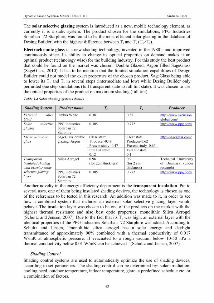
Solar shading systems Based on previous researches about existing products, but also looking into the development of new products fit for the purpose, four types of shading systems were considered and are presented in Table 3.4.
The external roller blinds system is a classic mobile shading solution, widely used at present. The specific product, Ombra White, was previously studied by Rosencrantz in his paper G-Values Of Solar Control Windows With Internal Solar Shading Devices (Rosencrantz, 2005), and proved to have good results in the overall performance.
Dynamic Facade Systems- Master Thesis, LTH Sînziana Râșca
32
The solar selective glazing system is introduced as a new, mobile technology element, as currently it is a static system. The product chosen for the simulations, PPG Industries Solarban 72 Starphire, was found to be the most efficient solar glazing in the database of Desing Builder, with the highest difference between Ts and Tv (Tv>Ts).
Electrochromic glass is a new shading technology, invented in the 1980’s and improved continuously since. Its ability to change its optical properties on demand makes it an optimal product (technology wise) for the building industry. For this study the best product that could be found on the market was chosen: Double Glazed, Argon filled SageGlass (SageGlass, 2010). It has to be mention that the limited simulation capabilities of Design Builder could not model the exact properties of the chosen product, SageGlass being able to lower its Tv and Ts in several steps (intermediate and low) while Desing Builder only permitted one step simulations (full transparent state to full tint state). It was chosen to use the optical properties of the product on maximum shading (full tint). Table 3.4 Solar shading systems details
Shading System Product name Ts Tv Producer
External roller blind
Ombra White 0.38 0.38 http://www.svenssonglobal.com/
Solar selective glazing
PPG Industries Solarban 72 Starphire
0.305 0.772 http://www.ppg.com/
Electro-chromic glass
SageGlass double glazing, Argon
Clear state: Producer-0.48 Present study- 0.47
Clear state: Producer-0.62 Present study- 0.66
http://sageglass.com/
Full tint state: 0.12
Full tint state: 0.1
Transparent insulated shading with exterior solar selective glazing layer
Silica Aerogel 0.96 (for 2cm thickness)
0.9 (for 2 cm thickness)
Technical University of Denmark (under research)
PPG Industries Solarban 72 Starphire
0.305 0.772 http://www.ppg.com/
Another novelty in the energy efficiency department is the transparent insulation. Put to several uses, one of them being insulated shading devices, the technology is chosen as one of the references to be tested in this research. An addition was made to it, in order to see how a combined system that includes an external solar selective glazing layer would behave. The insulation layer was chosen to be one of the products on the market with the highest thermal resistance and also best optic properties: monolithic Silica Aerogel (Schultz and Jensen, 2007). Due to the fact that its Ts was high, an external layer with the identical properties of the PPG Industries Solarban 72 Starphire was added. According to Schultz and Jensen, ”monolithic silica aerogel has a solar energy and daylight transmittance of approximately 90% combined with a thermal conductivity of 0.017 W/mK at atmospheric pressure. If evacuated to a rough vacuum below 10-50 hPa a thermal conductivity below 0.01 W/mK can be achieved” (Schultz and Jensen, 2007).
Shading Control Shading control systems are used to automatically optimize the use of shading devices, according to set parameters. The shading control can be determined by: solar irradiation, cooling need, outdoor temperature, indoor temperature, glare, a predefined schedule etc. or a combination of factors.
Dynamic Facade Systems- Master Thesis, LTH Sînziana Râșca
33
The choice of control systems has slight variations according to case. Initially, a number of control systems were tested on an XS size office building located in Chicago. Due to the fact that three of the four locations have a pronounced heating need, and therefore need to use the available solar irradiation during the winter time, the simulations are initially done for several control system for summer only and, for comparison, the same control systems are tested for the whole year. After assessing the results of the initial simulations, the number of tested control systems is reduced by eliminating the ones with poor results.
To limit the amount of information, the decision is taken to present simulation results only for the following control systems (as they are the ones with the best results):
- Solar, two solar set-point values (95 W/m2, 189 W/m2) - Schedule – always on - Day cooling, low outside temperature (under 12oC) - for insulated shading
only - Low outside temperature (under 12oC) - for insulated shading only.
The two solar set point values are selected based upon the study made by Wankanapona and Mistrickb, where three values were used as reference values for low (95 W/m2), medium (189 W/m2) and high (400 W/m2) solar set-point for automatic shading control (Wankanapona and Mistrickb, 2011). For all cases considered simulations are performed with four control systems for all types of shading devices (Solar 95-summer, Solar 189-summer, Solar 189- all year, On – all year). For Miami the insulating shading device is not tested there due to the lack of heating need.
Due to the fact that the shading devices influence the heating, cooling and lighting need, the only way to observe the savings achieved in a simple and realistic way is to transform the energy need in euro. The formula used to calculate the impact of the shading devices on the building: Savings (euro) = (Base Case Lighting Demand - Shading Device Lighting Demand +(Base Case Cooling Demand – Shading Device Cooling Demand)/CoP)*0.137 + ((Base Case Heating Demand – Shading Device Heating Demand)/CoP*0.8
Yearly impact estimation of the Dynamic Façade System For the present study, the impact of the Dynamic Façade System comprises of the behaviour of two factors:
- Opaque elements with variable U-value - Transparent elements with variable g-value.
In order to estimate the overall impact of the system on the building’s energy demand, a two steps approach was undertaken:
Step 1 – Calculate the impact of the shading system with the best results for the specific case
Step 2 – Add the estimated impact of the daily variable U-value (on the cooling need) to the results achieved in Step 1.
The results of this process could then be compared to the base case and the overall impact registered.
Dynamic Facade Systems- Master Thesis, LTH Sînziana Râșca
34
Computer simulation tools 3.2. Three computer simulation tools were used to study the behaviour of the buildings in different situations. The following section gives a short introduction to the employed tools and the reasons why they were chosen.
Global Heat Management Potential simulation tool (PHPP based) The Global Study on Heat Management Potential simulation software is a PHPP (Passive House Institute, 2012) based tool developed by LUWOGE Consult GmbH within the ”Global Study on Heat Management Potential” project. The program aims to be an estimation tool for building energy consumption and construction elements design (in respect to thermal properties). Focused mainly on three regions of the globe: USA, Europe and China, it offers the user a limited range of building uses, sizes, locations and desired energy levels that can be combined in the input phase, and recommends the necessary thermal resistance of the building components so that the building meets the chosen energy standard, also estimating the heating and cooling need and load.
The tool uses Microsoft Office Excel as a computing platform and is not a dynamic simulation tool. Also, a number of simplifications were made to its input data, thus the program giving a rough, but realistic estimation of the building’s energy performance.
In the present research, the tool is used for:
- Extracting data for the building typologies selected (dimensions, glazing surface, U-values, heat recovery efficiency etc.)
- Setting the benchmark for the estimation of heating and cooling needs for the respective buildings.
Design Builder Design Builder is an Energy Plus2 based dynamic simulation tool, developed by Design Builder Software Ltd. The software can be used for checking the building energy, carbon levels, lighting (using an advanced Radiance ray-tracing engine) and comfort performance. It allows to rapidly compare the function and performance of building designs [Design Builder, 2014], being a software approved for the following types of projects:
- Energy and comfort analysis - ASHRAE 90.1 Energy Cost Budget Analysis - BREEAM and LEED certification - Renewable energy strategy reports - Natural ventilation analysis and design advice - Condensation prediction and thermal bridging analysis - Actual and artificial light prediction and visualisation - Internal and external microclimate studies - UK-Energy Performance Certificates (level 3, 4 and 5)
2 EnergyPlus is an energy analysis and thermal load simulation program. It calculates heating and cooling loads necessary to maintain thermal control setpoints, conditions throughout a secondary HVAC system and coil loads, and the energy consumption of primary plant equipment.
Dynamic Facade Systems- Master Thesis, LTH Sînziana Râșca
35
- UK- Building Regulations Part L1 and L2 analysis - UK- Display Energy Certificates - UK- Code for Sustainable Homes.
The program considers the thermal mass in the simulations, but thermal bridges are not possible to model. Also, it offers the option of defining schedules for most variable elements of the building use (occupancy, internal gains, ventilation, heating and cooling etc.). An important element is that the latest version of the software, used in the present project, offers the possibility to use a heat-recovery system. In the present study Design Builder is used for the vast majority of simulations, such as:
- Estimate a more accurate heating and cooling demand for each case; - Estimate the lighting need according to case; - Estimate the impact of various shading devices on the heating, cooling and
lighting demand; - Estimate the overall impact of walls with season variable U-value in each location.
EDSL –Tas simulation software Tas is a building modelling and simulation tool, capable of performing dynamic thermal simulations. It allows designers to predict energy consumption, CO2 emissions, operating costs and occupant comfort (EDSL, 2012). Tas does not use any SBEM (simplified building energy model) type calculation procedures and so delivers design and compliance in one tool. One set-back for this program is that a ventilation system with heat recovery can only be implemented in the advance HVAC design part, which was not used in the present study (due to time limitations). Thus, a Microsoft Excel tool developed by LUWOGE Consult GmbH was used to simulate the heat recovery contribution to the energy demand of the building.
In what concerns the program’s accreditation, they are listed below:
- Part L2- CO2 calculations, solar gain checks and BRUKL documents - EPC Analysis (also accredited for Section 6 of Scottish Building Regulations) - analysing schools for summertime overheating compliance with Building Bulletin
101, as well as running overheating calculations on other building types - ASHRAE 90.1 (LEED) calculations - BREEAM - “Health and Well being” and “Energy” credits. Hea01 Visual comfort:
Daylighting calculation carried out to check for daylight factors, uniformity etc, Hea03 Thermal comfort: Thermal analysis to ensure thermal comfort levels are met.
As Design Builder, EDSL Tas considers thermal mass and offers the possibility of implementing schedules. Thermal bridges can not be modelled in it as well.
In the present research EDSL Tas is used for:
- Estimating the heating and cooling demand in each case (double-check Design Builder simulation results)
- Estimating the savings for cooling achieved with a daily variable U-value envelope.
Dynamic Facade Systems- Master Thesis, LTH Sînziana Râșca
36
Buildings data 4.
We expect too much of new buildings, and too little of ourselves.
(Jane Jacobs, 1961)

Dynamic Facade Systems- Master Thesis, LTH Sînziana Râșca
37
Dynamic Facade Systems- Master Thesis, LTH Sînziana Râșca
38
The building data considered will be presented in the following section, as it is an important element of the study. In what concerns the two chosen building uses, office and residential, they were selected as most representative for USA, Europe and China, as presented in the introduction chapter and highlighted in Figure 1.1. Information was extracted from the GSHMP project developed by LUWOGE consult GmbH.
The two building size typologies were selected from the seven steps scale defined in the GSHMP project (presented in Figure 1.2) as the most representative sizes for Europe, USA (XS- 380 m2 gross area) and China (L- 6000 m2 gross area). Figure 1.3 extracted from the same project presents the building distribution according to size in these three regions, and marks the average building size. The reasoning behind choosing the two sizes was not only that they are representative for the three regions, but also the wish of having two sizes closer to extremes, in order to be able to understand better the building behaviour for a wider range of possibilities.
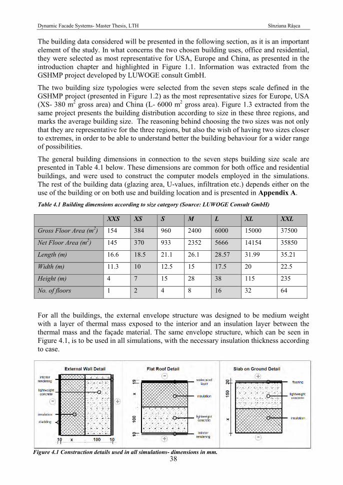
The general building dimensions in connection to the seven steps building size scale are presented in Table 4.1 below. These dimensions are common for both office and residential buildings, and were used to construct the computer models employed in the simulations. The rest of the building data (glazing area, U-values, infiltration etc.) depends either on the use of the building or on both use and building location and is presented in Appendix A. Table 4.1 Building dimensions according to size category (Source: LUWOGE Consult GmbH)
XXS XS S M L XL XXL
Gross Floor Area (m2) 154 384 960 2400 6000 15000 37500
Net Floor Area (m2) 145 370 933 2352 5666 14154 35850
Length (m) 16.6 18.5 21.1 26.1 28.57 31.99 35.21
Width (m) 11.3 10 12.5 15 17.5 20 22.5
Height (m) 4 7 15 28 38 115 235
No. of floors 1 2 4 8 16 32 64
For all the buildings, the external envelope structure was designed to be medium weight with a layer of thermal mass exposed to the interior and an insulation layer between the thermal mass and the façade material. The same envelope structure, which can be seen in Figure 4.1, is to be used in all simulations, with the necessary insulation thickness according to case.
Figure 4.1 Construction details used in all simulations- dimensions in mm.

Dynamic Facade Systems- Master Thesis, LTH Sînziana Râșca
39
Winds were not considered in any simulation, due to the complexity that this element would give to the study.
In what concerns possible refurbishments, they are considered only in the case of Level 5 buildings, where the simulations show what running cost reductions (heating and cooling) could be achieved if the building envelope would be refurbished with a Dynamic Façade System.

Dynamic Facade Systems- Master Thesis, LTH Sînziana Râșca
40
Results 5. Insanity: doing the same thing over and over again and expecting different results.
(A. Einstein)
Dynamic Facade Systems- Master Thesis, LTH Sînziana Râșca
41
This section presents the results achieved in each stage of the study. In order to limit the extent of the paper, but keep the essential information needed to perform the final analysis, for the following chapter the detailed results are only presented for the case of Chicago in most situations, as a representative case (the climate of Chicago is met in a wide range of locations across USA, Europe and China and its features- hot summers, cold winters, notable day to night temperature differences, high level of solar irradiation- make it one of the best candidates for a Dynamic Façade System).The detailed results for the rest of the locations is available for consultation in the Appendix section.
All results that are presented in W/m2, Wh/m2/day, kWh/m2/year refer to the final energy need. The only cases where the final energy is transformed into net-energy and then in euro/m2/year are in the results that present the impact of the variable g-value and in the calculation of the overall impact of the Dynamic Façade System. Minimizing the number of situations where the results were transformed to euros was done based on two reasons: have a common comparison value between different energy demands (cooling, heating, lighting) and in order to simplify the calculation complexity (avoid performing too many transformations and thus leave more room for errors), due to the fact that the simulation tools used give results for the final energy need.
Base cases 5.1. For all base cases the simulations were performed with Design Builder. The input data used in all simulations can be found in Appendix A. The results are presented separately for XS-size building and L-size ones, so that they can be easily comparable.
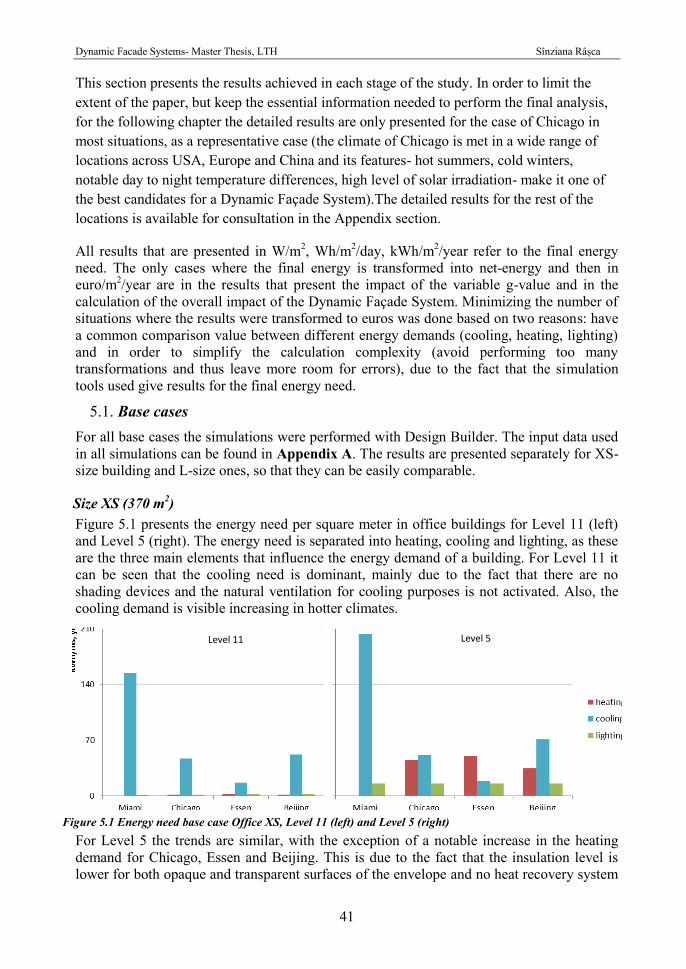
Size XS (370 m2) Figure 5.1 presents the energy need per square meter in office buildings for Level 11 (left) and Level 5 (right). The energy need is separated into heating, cooling and lighting, as these are the three main elements that influence the energy demand of a building. For Level 11 it can be seen that the cooling need is dominant, mainly due to the fact that there are no shading devices and the natural ventilation for cooling purposes is not activated. Also, the cooling demand is visible increasing in hotter climates.
For Level 5 the trends are similar, with the exception of a notable increase in the heating demand for Chicago, Essen and Beijing. This is due to the fact that the insulation level is lower for both opaque and transparent surfaces of the envelope and no heat recovery system
Figure 5.1 Energy need base case Office XS, Level 11 (left) and Level 5 (right)
Level 11 Level 5
Dynamic Facade Systems- Master Thesis, LTH Sînziana Râșca
42
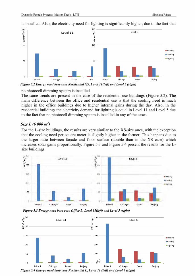
is installed. Also, the electricity need for lighting is significantly higher, due to the fact that
no photocell dimming system is installed. The same trends are present in the case of the residential use buildings (Figure 5.2). The main difference between the office and residential use is that the cooling need is much higher in the office buildings due to higher internal gains during the day. Also, in the residential buildings the electricity demand for lighting is equal in Level 11 and Level 5 due to the fact that no photocell dimming system is installed in any of the cases.
Size L (6 000 m2) For the L-size buildings, the results are very similar to the XS-size ones, with the exception that the cooling need per square meter is slightly higher in the former. This happens due to the larger ratio between façade and floor surface (double than in the XS case) which increases solar gains proportionally. Figure 5.3 and Figure 5.4 present the results for the L-size buildings.
Figure 5.2 Energy need base case Residential XS, Level 11(left) and Level 5 (right)
Figure 5.4 Energy need base case Residential L, Level 11 (left) and Level 5 (right)
Figure 5.3 Energy need base case Office L, Level 11(left) and Level 5 (right)
Dynamic Facade Systems- Master Thesis, LTH Sînziana Râșca
43
Seasonal variation of U-value 5.2. The results presented in this section show the impact of the seasonal variation of the U-value in the opaque elements of the envelope of the studied buildings. Detailed graphs of the yearly analysis for each location and building use are presented in Appendix C.
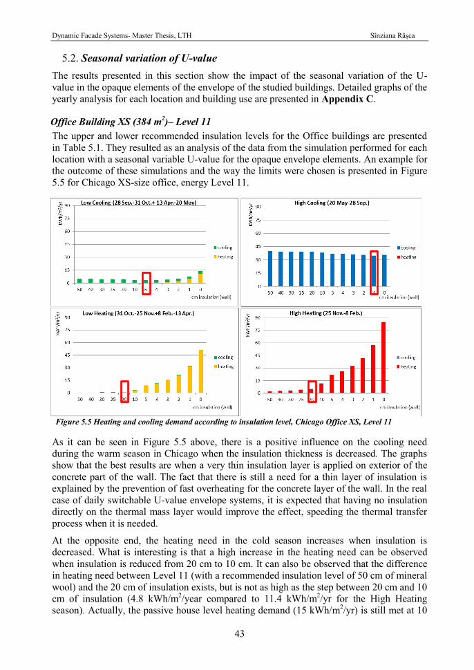
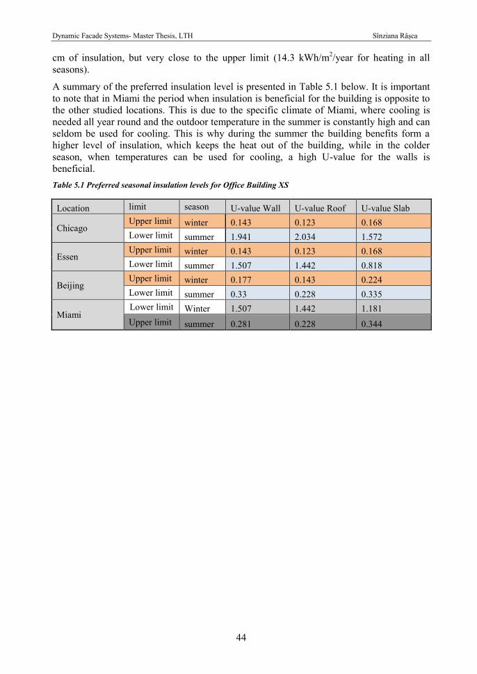
Office Building XS (384 m2)– Level 11 The upper and lower recommended insulation levels for the Office buildings are presented in Table 5.1. They resulted as an analysis of the data from the simulation performed for each location with a seasonal variable U-value for the opaque envelope elements. An example for the outcome of these simulations and the way the limits were chosen is presented in Figure 5.5 for Chicago XS-size office, energy Level 11.
As it can be seen in Figure 5.5 above, there is a positive influence on the cooling need during the warm season in Chicago when the insulation thickness is decreased. The graphs show that the best results are when a very thin insulation layer is applied on exterior of the concrete part of the wall. The fact that there is still a need for a thin layer of insulation is explained by the prevention of fast overheating for the concrete layer of the wall. In the real case of daily switchable U-value envelope systems, it is expected that having no insulation directly on the thermal mass layer would improve the effect, speeding the thermal transfer process when it is needed.
At the opposite end, the heating need in the cold season increases when insulation is decreased. What is interesting is that a high increase in the heating need can be observed when insulation is reduced from 20 cm to 10 cm. It can also be observed that the difference in heating need between Level 11 (with a recommended insulation level of 50 cm of mineral wool) and the 20 cm of insulation exists, but is not as high as the step between 20 cm and 10 cm of insulation (4.8 kWh/m2/year compared to 11.4 kWh/m2/yr for the High Heating season). Actually, the passive house level heating demand (15 kWh/m2/yr) is still met at 10
Figure 5.5 Heating and cooling demand according to insulation level, Chicago Office XS, Level 11
Dynamic Facade Systems- Master Thesis, LTH Sînziana Râșca
44
cm of insulation, but very close to the upper limit (14.3 kWh/m2/year for heating in all seasons).
A summary of the preferred insulation level is presented in Table 5.1 below. It is important to note that in Miami the period when insulation is beneficial for the building is opposite to the other studied locations. This is due to the specific climate of Miami, where cooling is needed all year round and the outdoor temperature in the summer is constantly high and can seldom be used for cooling. This is why during the summer the building benefits form a higher level of insulation, which keeps the heat out of the building, while in the colder season, when temperatures can be used for cooling, a high U-value for the walls is beneficial. Table 5.1 Preferred seasonal insulation levels for Office Building XS
Location limit season U-value Wall U-value Roof U-value Slab
Chicago Upper limit winter 0.143 0.123 0.168 Lower limit summer 1.941 2.034 1.572
Essen Upper limit winter 0.143 0.123 0.168 Lower limit summer 1.507 1.442 0.818
Beijing Upper limit winter 0.177 0.143 0.224 Lower limit summer 0.33 0.228 0.335
Miami Lower limit Winter 1.507 1.442 1.181 Upper limit summer 0.281 0.228 0.344
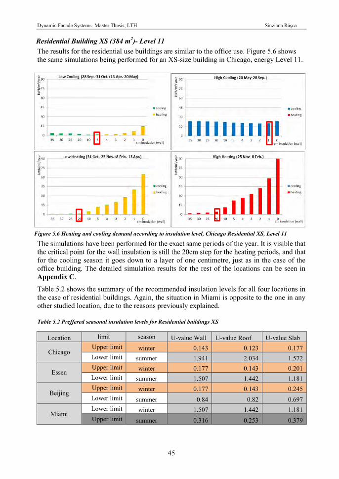
Dynamic Facade Systems- Master Thesis, LTH Sînziana Râșca
45
Residential Building XS (384 m2)- Level 11 The results for the residential use buildings are similar to the office use. Figure 5.6 shows the same simulations being performed for an XS-size building in Chicago, energy Level 11.
The simulations have been performed for the exact same periods of the year. It is visible that the critical point for the wall insulation is still the 20cm step for the heating periods, and that for the cooling season it goes down to a layer of one centimetre, just as in the case of the office building. The detailed simulation results for the rest of the locations can be seen in Appendix C.
Table 5.2 shows the summary of the recommended insulation levels for all four locations in the case of residential buildings. Again, the situation in Miami is opposite to the one in any other studied location, due to the reasons previously explained. Table 5.2 Preffered seasonal insulation levels for Residential buildings XS
Location limit season U-value Wall U-value Roof U-value Slab
Chicago Upper limit winter 0.143 0.123 0.177 Lower limit summer 1.941 2.034 1.572
Essen Upper limit winter 0.177 0.143 0.201 Lower limit summer 1.507 1.442 1.181
Beijing Upper limit winter 0.177 0.143 0.245 Lower limit summer 0.84 0.82 0.697
Miami Lower limit winter 1.507 1.442 1.181 Upper limit summer 0.316 0.253 0.379
Figure 5.6 Heating and cooling demand according to insulation level, Chicago Residential XS, Level 11
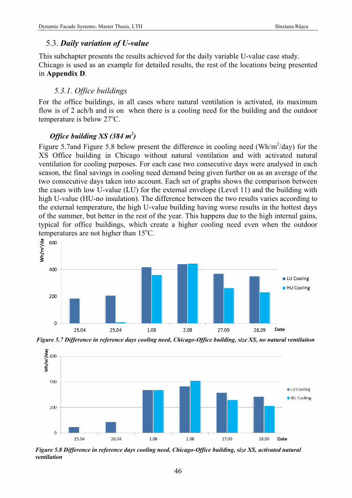
Dynamic Facade Systems- Master Thesis, LTH Sînziana Râșca
46
Daily variation of U-value 5.3. This subchapter presents the results achieved for the daily variable U-value case study. Chicago is used as an example for detailed results, the rest of the locations being presented in Appendix D.
5.3.1. Office buildings For the office buildings, in all cases where natural ventilation is activated, its maximum flow is of 2 ach/h and is on when there is a cooling need for the building and the outdoor temperature is below 27oC.
Office building XS (384 m2) Figure 5.7and Figure 5.8 below present the difference in cooling need (Wh/m2/day) for the XS Office building in Chicago without natural ventilation and with activated natural ventilation for cooling purposes. For each case two consecutive days were analysed in each season, the final savings in cooling need demand being given further on as an average of the two consecutive days taken into account. Each set of graphs shows the comparison between the cases with low U-value (LU) for the external envelope (Level 11) and the building with high U-value (HU-no insulation). The difference between the two results varies according to the external temperature, the high U-value building having worse results in the hottest days of the summer, but better in the rest of the year. This happens due to the high internal gains, typical for office buildings, which create a higher cooling need even when the outdoor temperatures are not higher than 15oC.
Figure 5.7 Difference in reference days cooling need, Chicago-Office building, size XS, no natural ventilation
Figure 5.8 Difference in reference days cooling need, Chicago-Office building, size XS, activated natural ventilation
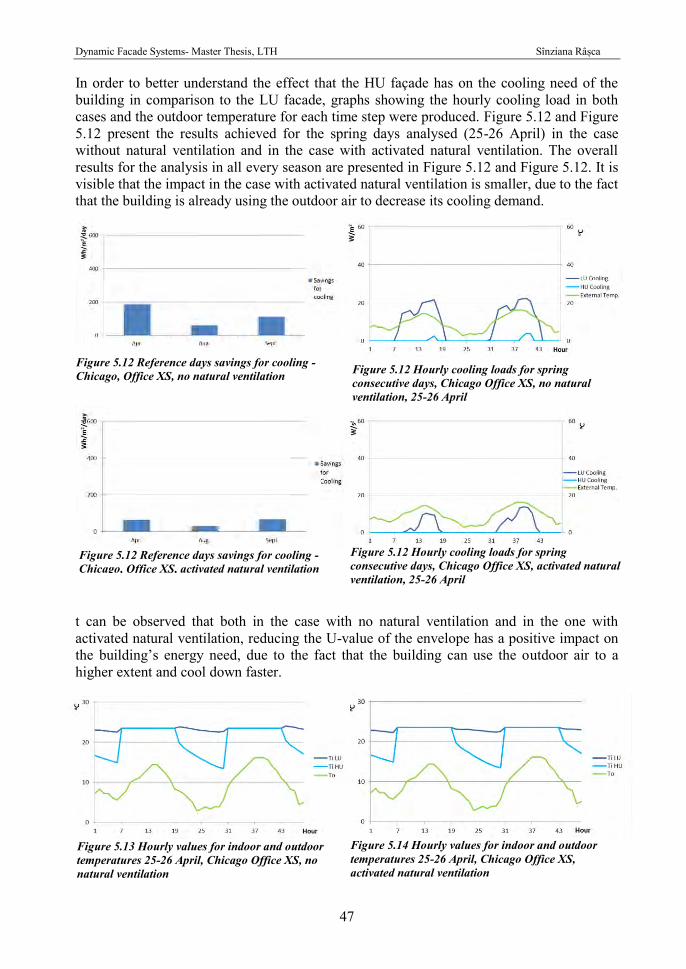
Dynamic Facade Systems- Master Thesis, LTH Sînziana Râșca
47
In order to better understand the effect that the HU façade has on the cooling need of the building in comparison to the LU facade, graphs showing the hourly cooling load in both cases and the outdoor temperature for each time step were produced. Figure 5.12 and Figure 5.12 present the results achieved for the spring days analysed (25-26 April) in the case without natural ventilation and in the case with activated natural ventilation. The overall results for the analysis in all every season are presented in Figure 5.12 and Figure 5.12. It is visible that the impact in the case with activated natural ventilation is smaller, due to the fact that the building is already using the outdoor air to decrease its cooling demand.
t can be observed that both in the case with no natural ventilation and in the one with activated natural ventilation, reducing the U-value of the envelope has a positive impact on the building’s energy need, due to the fact that the building can use the outdoor air to a higher extent and cool down faster.
Figure 5.14 Hourly values for indoor and outdoor temperatures 25-26 April, Chicago Office XS, activated natural ventilation
Figure 5.12 Reference days savings for cooling - Chicago, Office XS, no natural ventilation
Figure 5.12 Reference days savings for cooling - Chicago, Office XS, activated natural ventilation
Figure 5.12 Hourly cooling loads for spring consecutive days, Chicago Office XS, activated natural ventilation, 25-26 April
Figure 5.12 Hourly cooling loads for spring consecutive days, Chicago Office XS, no natural ventilation, 25-26 April
Figure 5.13 Hourly values for indoor and outdoor temperatures 25-26 April, Chicago Office XS, no natural ventilation
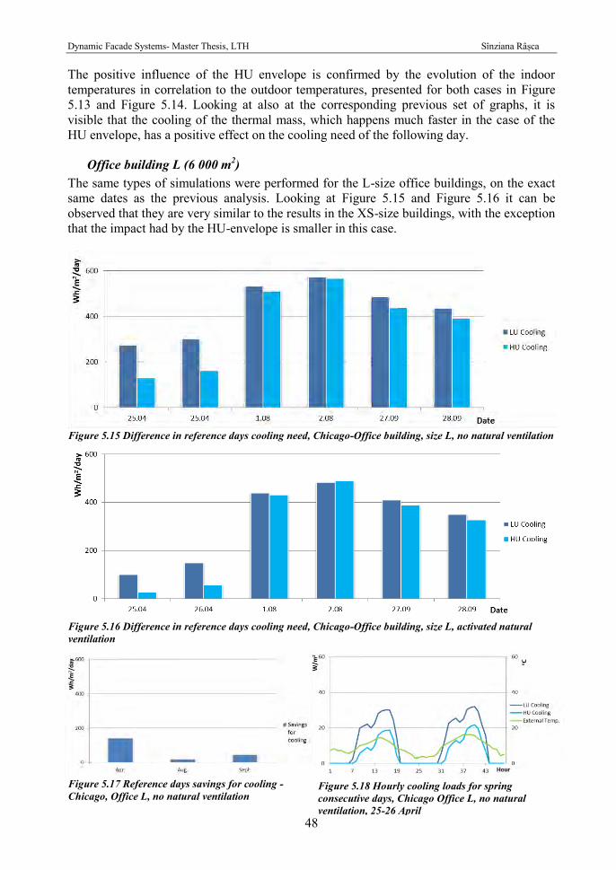
Dynamic Facade Systems- Master Thesis, LTH Sînziana Râșca
48
The positive influence of the HU envelope is confirmed by the evolution of the indoor temperatures in correlation to the outdoor temperatures, presented for both cases in Figure 5.13 and Figure 5.14. Looking at also at the corresponding previous set of graphs, it is visible that the cooling of the thermal mass, which happens much faster in the case of the HU envelope, has a positive effect on the cooling need of the following day.
Office building L (6 000 m2) The same types of simulations were performed for the L-size office buildings, on the exact same dates as the previous analysis. Looking at Figure 5.15 and Figure 5.16 it can be observed that they are very similar to the results in the XS-size buildings, with the exception that the impact had by the HU-envelope is smaller in this case.
Figure 5.15 Difference in reference days cooling need, Chicago-Office building, size L, no natural ventilation
Figure 5.16 Difference in reference days cooling need, Chicago-Office building, size L, activated natural ventilation
Figure 5.18 Hourly cooling loads for spring consecutive days, Chicago Office L, no natural ventilation, 25-26 April
Figure 5.17 Reference days savings for cooling - Chicago, Office L, no natural ventilation
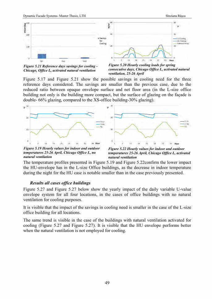
Dynamic Facade Systems- Master Thesis, LTH Sînziana Râșca
49
Figure 5.17 and Figure 5.21 show the possible savings in cooling need for the three reference days considered. The savings are smaller than the previous case, due to the reduced ratio between opaque envelope surface and net floor area (in the L-size office building not only is the building more compact, but the surface of glazing on the façade is double- 66% glazing, compared to the XS-office building-30% glazing).
The temperature profiles presented in Figure 5.19 and Figure 5.22confirm the lower impact the HU-envelope has in the L-size Office buildings, as the decrease in indoor temperature during the night for the HU case is notable smaller than in the case previously presented.
Results all cases office buildings Figure 5.27 and Figure 5.27 below show the yearly impact of the daily variable U-value envelope system for all four locations, in the cases of office buildings with no natural ventilation for cooling purposes.
It is visible that the impact of the savings in cooling need is smaller in the case of the L-size office building for all locations.
The same trend is visible in the case of the buildings with natural ventilation activated for cooling (Figure 5.27 and Figure 5.27). It is visible that the HU envelope performs better when the natural ventilation is not employed for cooling.
Figure 5.22 Hourly values for indoor and outdoor temperatures 25-26 April, Chicago Office L, activated natural ventilation
Figure 5.20 Hourly cooling loads for spring consecutive days, Chicago Office L, activated natural ventilation, 25-26 April
Figure 5.21 Reference days savings for cooling - Chicago, Office L, activated natural ventilation
Figure 5.19 Hourly values for indoor and outdoor temperatures 25-26 April, Chicago Office L, no natural ventilation
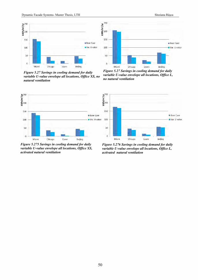
Dynamic Facade Systems- Master Thesis, LTH Sînziana Râșca
50
Figure 5.27 Savings in cooling demand for daily variable U-value envelope all locations, Office XS, no natural ventilation
Figure 5.27 Savings in cooling demand for daily variable U-value envelope all locations, Office L, no natural ventilation
Figure 5.275 Savings in cooling demand for daily variable U-value envelope all locations, Office XS, activated natural ventilation
Figure 5.276 Savings in cooling demand for daily variable U-value envelope all locations, Office L, activated natural ventilation
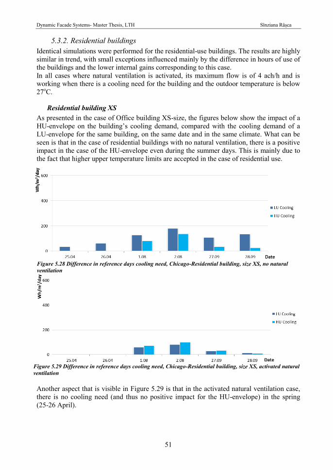
Dynamic Facade Systems- Master Thesis, LTH Sînziana Râșca
51
5.3.2. Residential buildings Identical simulations were performed for the residential-use buildings. The results are highly similar in trend, with small exceptions influenced mainly by the difference in hours of use of the buildings and the lower internal gains corresponding to this case. In all cases where natural ventilation is activated, its maximum flow is of 4 ach/h and is working when there is a cooling need for the building and the outdoor temperature is below 27oC.
Residential building XS As presented in the case of Office building XS-size, the figures below show the impact of a HU-envelope on the building’s cooling demand, compared with the cooling demand of a LU-envelope for the same building, on the same date and in the same climate. What can be seen is that in the case of residential buildings with no natural ventilation, there is a positive impact in the case of the HU-envelope even during the summer days. This is mainly due to the fact that higher upper temperature limits are accepted in the case of residential use.
Another aspect that is visible in Figure 5.29 is that in the activated natural ventilation case, there is no cooling need (and thus no positive impact for the HU-envelope) in the spring (25-26 April).
Figure 5.28 Difference in reference days cooling need, Chicago-Residential building, size XS, no natural ventilation
Figure 5.29 Difference in reference days cooling need, Chicago-Residential building, size XS, activated natural ventilation
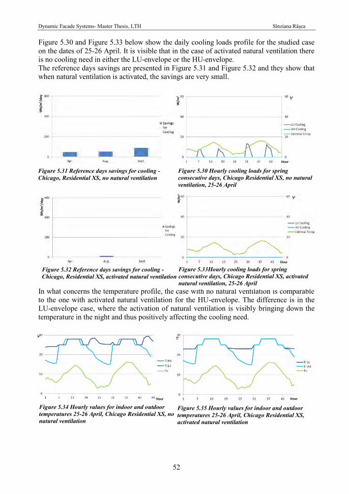
Dynamic Facade Systems- Master Thesis, LTH Sînziana Râșca
52
Figure 5.30 and Figure 5.33 below show the daily cooling loads profile for the studied case on the dates of 25-26 April. It is visible that in the case of activated natural ventilation there is no cooling need in either the LU-envelope or the HU-envelope. The reference days savings are presented in Figure 5.31 and Figure 5.32 and they show that when natural ventilation is activated, the savings are very small.
In what concerns the temperature profile, the case with no natural ventilation is comparable to the one with activated natural ventilation for the HU-envelope. The difference is in the LU-envelope case, where the activation of natural ventilation is visibly bringing down the temperature in the night and thus positively affecting the cooling need.
Figure 5.32 Reference days savings for cooling - Chicago, Residential XS, activated natural ventilation
Figure 5.31 Reference days savings for cooling - Chicago, Residential XS, no natural ventilation
Figure 5.30 Hourly cooling loads for spring consecutive days, Chicago Residential XS, no natural ventilation, 25-26 April
Figure 5.33Hourly cooling loads for spring consecutive days, Chicago Residential XS, activated natural ventilation, 25-26 April
Figure 5.34 Hourly values for indoor and outdoor temperatures 25-26 April, Chicago Residential XS, no natural ventilation
Figure 5.35 Hourly values for indoor and outdoor temperatures 25-26 April, Chicago Residential XS, activated natural ventilation
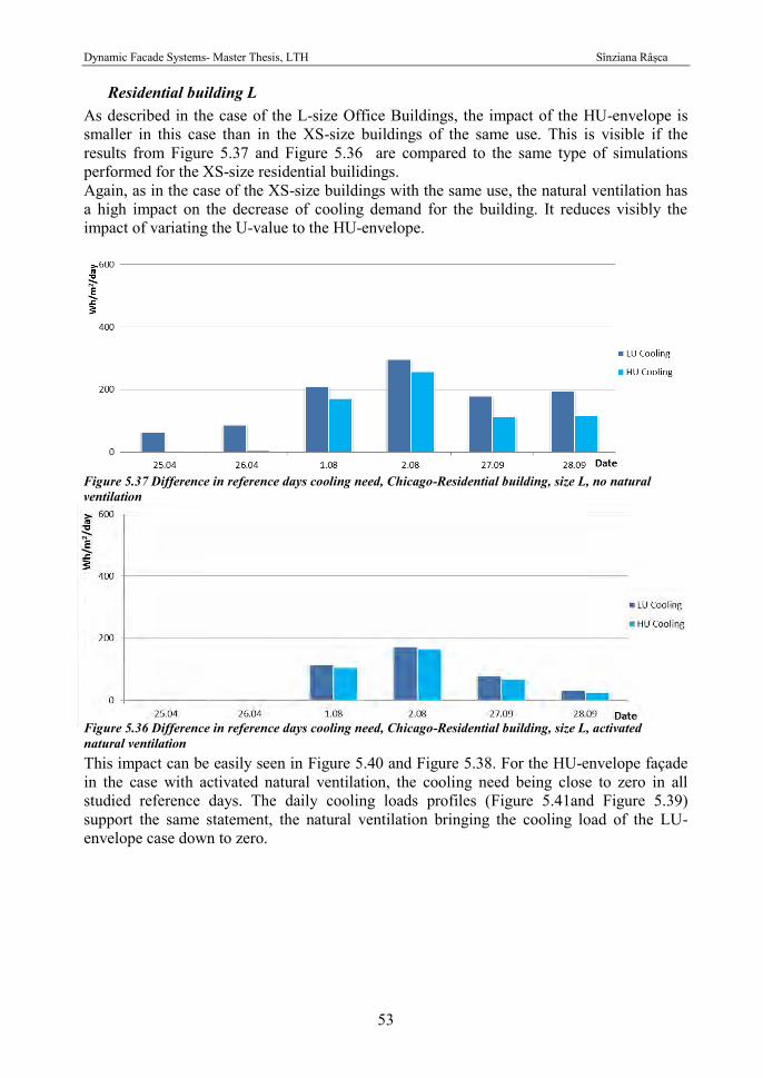
Dynamic Facade Systems- Master Thesis, LTH Sînziana Râșca
53
Residential building L As described in the case of the L-size Office Buildings, the impact of the HU-envelope is smaller in this case than in the XS-size buildings of the same use. This is visible if the results from Figure 5.37 and Figure 5.36 are compared to the same type of simulations performed for the XS-size residential builidings. Again, as in the case of the XS-size buildings with the same use, the natural ventilation has a high impact on the decrease of cooling demand for the building. It reduces visibly the impact of variating the U-value to the HU-envelope.
This impact can be easily seen in Figure 5.40 and Figure 5.38. For the HU-envelope façade in the case with activated natural ventilation, the cooling need being close to zero in all studied reference days. The daily cooling loads profiles (Figure 5.41and Figure 5.39) support the same statement, the natural ventilation bringing the cooling load of the LU-envelope case down to zero.
Figure 5.37 Difference in reference days cooling need, Chicago-Residential building, size L, no natural ventilation
Figure 5.36 Difference in reference days cooling need, Chicago-Residential building, size L, activated natural ventilation
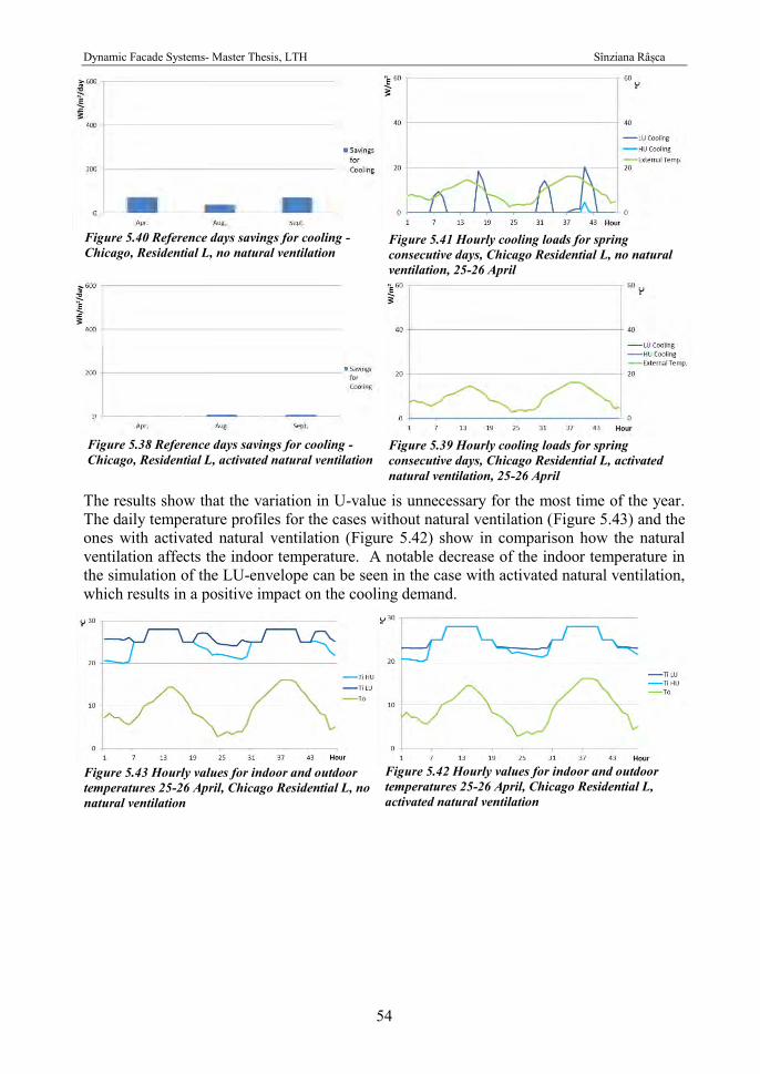
Dynamic Facade Systems- Master Thesis, LTH Sînziana Râșca
54
The results show that the variation in U-value is unnecessary for the most time of the year. The daily temperature profiles for the cases without natural ventilation (Figure 5.43) and the ones with activated natural ventilation (Figure 5.42) show in comparison how the natural ventilation affects the indoor temperature. A notable decrease of the indoor temperature in the simulation of the LU-envelope can be seen in the case with activated natural ventilation, which results in a positive impact on the cooling demand.
Figure 5.40 Reference days savings for cooling - Chicago, Residential L, no natural ventilation
Figure 5.41 Hourly cooling loads for spring consecutive days, Chicago Residential L, no natural ventilation, 25-26 April
Figure 5.38 Reference days savings for cooling - Chicago, Residential L, activated natural ventilation
Figure 5.39 Hourly cooling loads for spring consecutive days, Chicago Residential L, activated natural ventilation, 25-26 April
Figure 5.43 Hourly values for indoor and outdoor temperatures 25-26 April, Chicago Residential L, no natural ventilation
Figure 5.42 Hourly values for indoor and outdoor temperatures 25-26 April, Chicago Residential L, activated natural ventilation
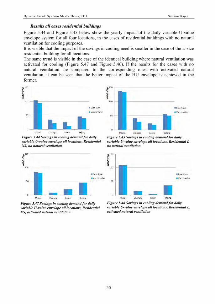
Dynamic Facade Systems- Master Thesis, LTH Sînziana Râșca
55
Results all cases residential buildings Figure 5.44 and Figure 5.45 below show the yearly impact of the daily variable U-value envelope system for all four locations, in the cases of residential buildings with no natural ventilation for cooling purposes. It is visible that the impact of the savings in cooling need is smaller in the case of the L-size residential building for all locations. The same trend is visible in the case of the identical building where natural ventilation was activated for cooling (Figure 5.47 and Figure 5.46). If the results for the cases with no natural ventilation are compared to the corresponding ones with activated natural ventilation, it can be seen that the better impact of the HU envelope is achieved in the former.
Figure 5.44 Savings in cooling demand for daily variable U-value envelope all locations, Residential XS, no natural ventilation
Figure 5.47 Savings in cooling demand for daily variable U-value envelope all locations, Residential XS, activated natural ventilation
Figure 5.46 Savings in cooling demand for daily variable U-value envelope all locations, Residential L, activated natural ventilation
Figure 5.45 Savings in cooling demand for daily variable U-value envelope all locations, Residential L no natural ventilation
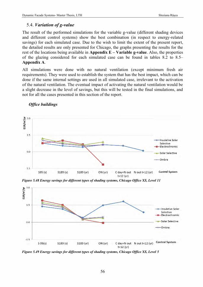
Dynamic Facade Systems- Master Thesis, LTH Sînziana Râșca
56
Variation of g-value 5.4. The result of the performed simulations for the variable g-value (different shading devices and different control systems) show the best combination (in respect to energy-related savings) for each simulated case. Due to the wish to limit the extent of the present report, the detailed results are only presented for Chicago, the graphs presenting the results for the rest of the locations being available in Appendix E – Variable g-value. Also, the properties of the glazing considered for each simulated case can be found in tables 8.2 to 8.5– Appendix A.
All simulations were done with no natural ventilation (except minimum fresh air requirements). They were used to establish the system that has the best impact, which can be done if the same internal settings are used in all simulated case, irrelevant to the activation of the natural ventilation. The eventual impact of activating the natural ventilation would be a slight decrease in the level of savings, but this will be tested in the final simulations, and not for all the cases presented in this section of the report.
Office buildings
Figure 5.48 Energy savings for different types of shading systems, Chicago Office XS, Level 11
Figure 5.49 Energy savings for different types of shading systems, Chicago Office XS, Level 5
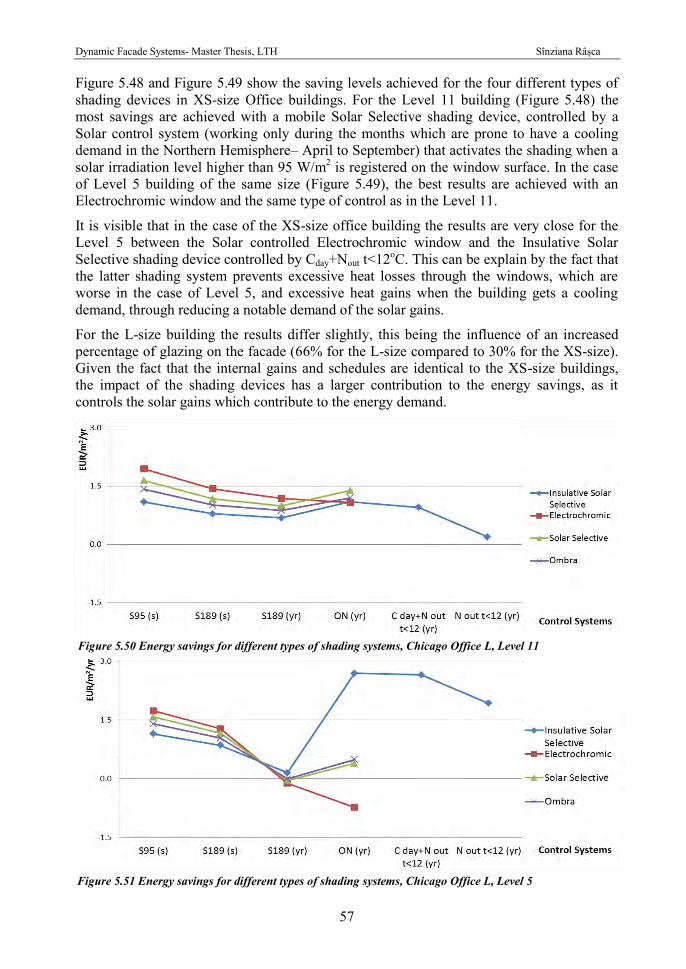
Dynamic Facade Systems- Master Thesis, LTH Sînziana Râșca
57
Figure 5.48 and Figure 5.49 show the saving levels achieved for the four different types of shading devices in XS-size Office buildings. For the Level 11 building (Figure 5.48) the most savings are achieved with a mobile Solar Selective shading device, controlled by a Solar control system (working only during the months which are prone to have a cooling demand in the Northern Hemisphere– April to September) that activates the shading when a solar irradiation level higher than 95 W/m2 is registered on the window surface. In the case of Level 5 building of the same size (Figure 5.49), the best results are achieved with an Electrochromic window and the same type of control as in the Level 11.
It is visible that in the case of the XS-size office building the results are very close for the Level 5 between the Solar controlled Electrochromic window and the Insulative Solar Selective shading device controlled by Cday+Nout t<12oC. This can be explain by the fact that the latter shading system prevents excessive heat losses through the windows, which are worse in the case of Level 5, and excessive heat gains when the building gets a cooling demand, through reducing a notable demand of the solar gains.
For the L-size building the results differ slightly, this being the influence of an increased percentage of glazing on the facade (66% for the L-size compared to 30% for the XS-size). Given the fact that the internal gains and schedules are identical to the XS-size buildings, the impact of the shading devices has a larger contribution to the energy savings, as it controls the solar gains which contribute to the energy demand.
Figure 5.51 Energy savings for different types of shading systems, Chicago Office L, Level 5
Figure 5.50 Energy savings for different types of shading systems, Chicago Office L, Level 11
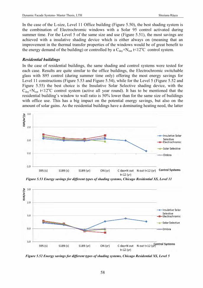
Dynamic Facade Systems- Master Thesis, LTH Sînziana Râșca
58
In the case of the L-size, Level 11 Office building (Figure 5.50), the best shading system is the combination of Electrochromic windows with a Solar 95 control activated during summer time. For the Level 5 of the same size and use (Figure 5.51), the most savings are achieved with a insulative shading device which is either always on (meaning that an improvement in the thermal transfer properties of the windows would be of great benefit to the energy demand of the building) or controlled by a Cday+Nout t<12oC control system.
Residential buildings In the case of residential buildings, the same shading and control systems were tested for each case. Results are quite similar to the office buildings, the Electrochromic switchable glass with S95 control (during summer time only) offering the most energy savings for Level 11 constructions (Figure 5.53 and Figure 5.54), while for the Level 5 (Figure 5.52 and Figure 5.55) the best choice is the Insulative Solar Selective shading device, with the Cday+Nout t<12oC control system (active all year round). It has to be mentioned that the residential building’s window to wall ratio is 50% lower than for the same size of buildings with office use. This has a big impact on the potential energy savings, but also on the amount of solar gains. As the residential buildings have a dominating heating need, the latter
Figure 5.53 Energy savings for different types of shading systems, Chicago Residential XS, Level 11
Figure 5.52 Energy savings for different types of shading systems, Chicago Residential XS, Level 5
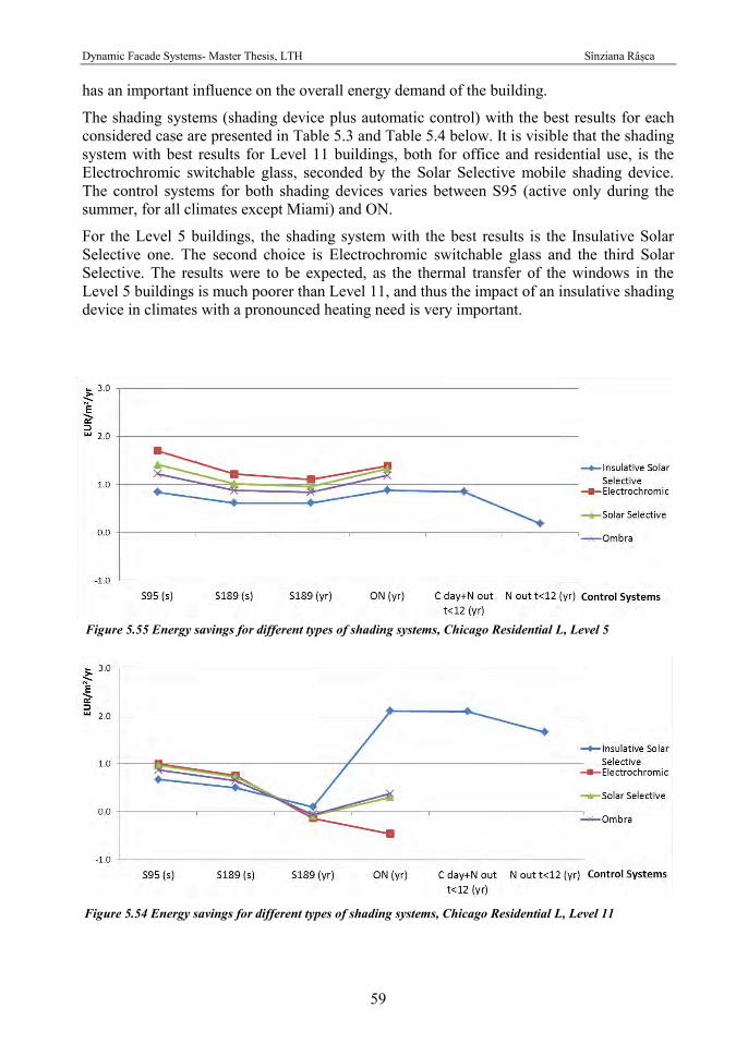
Dynamic Facade Systems- Master Thesis, LTH Sînziana Râșca
59
has an important influence on the overall energy demand of the building.
The shading systems (shading device plus automatic control) with the best results for each considered case are presented in Table 5.3 and Table 5.4 below. It is visible that the shading system with best results for Level 11 buildings, both for office and residential use, is the Electrochromic switchable glass, seconded by the Solar Selective mobile shading device. The control systems for both shading devices varies between S95 (active only during the summer, for all climates except Miami) and ON.
For the Level 5 buildings, the shading system with the best results is the Insulative Solar Selective one. The second choice is Electrochromic switchable glass and the third Solar Selective. The results were to be expected, as the thermal transfer of the windows in the Level 5 buildings is much poorer than Level 11, and thus the impact of an insulative shading device in climates with a pronounced heating need is very important.
Figure 5.55 Energy savings for different types of shading systems, Chicago Residential L, Level 5
Figure 5.54 Energy savings for different types of shading systems, Chicago Residential L, Level 11
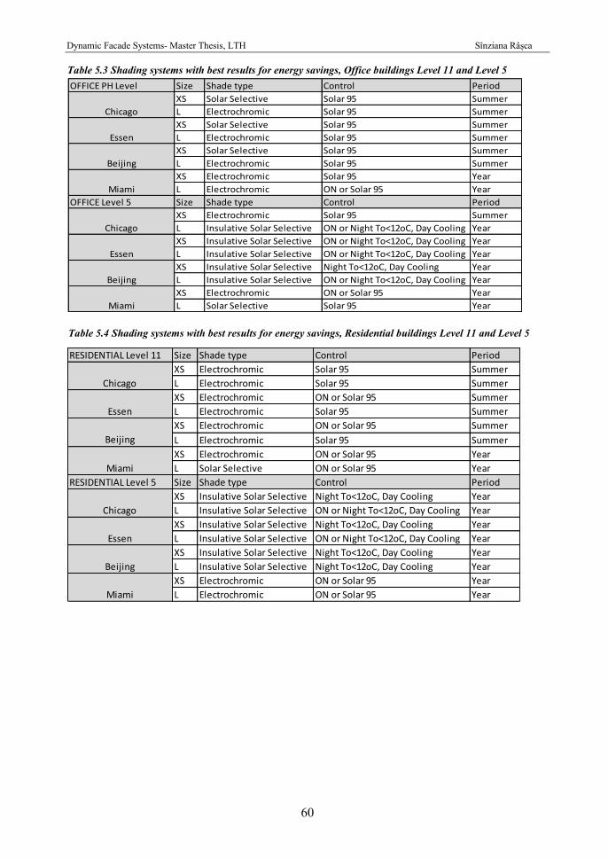
Dynamic Facade Systems- Master Thesis, LTH Sînziana Râșca
60
Table 5.3 Shading systems with best results for energy savings, Office buildings Level 11 and Level 5 OFFICE PH Level Size Shade type Control Period
XS Solar Selective Solar 95 Summer
L Electrochromic Solar 95 Summer
XS Solar Selective Solar 95 Summer
L Electrochromic Solar 95 Summer
XS Solar Selective Solar 95 Summer
L Electrochromic Solar 95 Summer
XS Electrochromic Solar 95 Year
L Electrochromic ON or Solar 95 Year
OFFICE Level 5 Size Shade type Control Period
XS Electrochromic Solar 95 Summer
L Insulative Solar Selective ON or Night To<12oC, Day Cooling Year
XS Insulative Solar Selective ON or Night To<12oC, Day Cooling Year
L Insulative Solar Selective ON or Night To<12oC, Day Cooling Year
XS Insulative Solar Selective Night To<12oC, Day Cooling Year
L Insulative Solar Selective ON or Night To<12oC, Day Cooling Year
XS Electrochromic ON or Solar 95 Year
L Solar Selective Solar 95 Year
Essen
Beijing
Miami
Chicago
Essen
Beijing
Miami
Chicago
RESIDENTIAL Level 11 Size Shade type Control Period
XS Electrochromic Solar 95 Summer
L Electrochromic Solar 95 Summer
XS Electrochromic ON or Solar 95 Summer
L Electrochromic Solar 95 Summer
XS Electrochromic ON or Solar 95 Summer
L Electrochromic Solar 95 Summer
XS Electrochromic ON or Solar 95 Year
L Solar Selective ON or Solar 95 Year
RESIDENTIAL Level 5 Size Shade type Control Period
XS Insulative Solar Selective Night To<12oC, Day Cooling Year
L Insulative Solar Selective ON or Night To<12oC, Day Cooling Year
XS Insulative Solar Selective Night To<12oC, Day Cooling Year
L Insulative Solar Selective ON or Night To<12oC, Day Cooling Year
XS Insulative Solar Selective Night To<12oC, Day Cooling Year
L Insulative Solar Selective Night To<12oC, Day Cooling Year
XS Electrochromic ON or Solar 95 Year
L Electrochromic ON or Solar 95 Year
Chicago
Essen
Beijing
Miami
Chicago
Essen
Beijing
Miami
Table 5.4 Shading systems with best results for energy savings, Residential buildings Level 11 and Level 5
Dynamic Facade Systems- Master Thesis, LTH Sînziana Râșca
61
Estimated yearly impact of the Dynamic Façade System 5.5. The following section presents the impact of the dynamic façade systems on passive house (Level 11) energy level, office and residential use buildings in all four studied locations. The energy demand for heating, cooling and lighting is transformed into net-energy and then in euro/m2/year. This choice of presenting the results was taken in order to have a common comparison value between different energy demands (cooling, heating, lighting).
The yearly impact of dynamic façade systems is only studied for new buildings of Level 11 (passive house) standards. This is done due to time limitations and the fact that in the case of building refurbishments installing a dynamic façade system has a complex approach, mainly in what concerns the variable U-value of the envelope (the lower limit of the U-value variation being constrained by the structure of the existing envelope).
In order to estimate the possible impact of a Dynamic Façade System, for each location and building type (size and use) an ideal case, based on the results achieved for the variation of the g-value and the daily variation of the U-value, was chosen. Error! Reference source ot found. presents the features of the façade used in the final calculation for the:
-maximum U-value of the walls, calculated in the season variable U-value section of the study (section 5.2);
-estimated yearly decrease in energy need for the specific case given by the daily variable U-value calculation (section 5.3);
-shading device and shading control with the best results for the case, resulting from the variable g-value simulations (section 5.4).
It can be observed that in the case of all buildings the impact of the dynamic facade systems varies not only according to location, but also according to the size of the building, due to the ratio between facade and floor area (bigger in the case of XS-size buildings, which means better results for the variable U-value than for the L-size buildings with the same use) and the ratio between windows and facade area (the values for each building type in this field can be checked in Appendix A- Input Data).
In all graphs, for each location three cases are presented:
- Base case (blue column) – Level 11, no shading system; - Base case with shading (green column) – Level 11, shading system active; - Dynamic façade (red column) – Level 11 with both shading and variable U-
value for the envelope active.
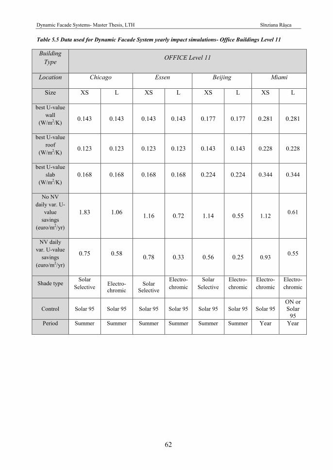
Dynamic Facade Systems- Master Thesis, LTH Sînziana Râșca
62
Table 5.5 Data used for Dynamic Facade System yearly impact simulations- Office Buildings Level 11
Building Type
OFFICE Level 11
Location Chicago Essen Beijing Miami
Size XS L XS L XS L XS L
best U-value wall
(W/m2/K) 0.143 0.143 0.143 0.143 0.177 0.177 0.281 0.281
best U-value roof
(W/m2/K) 0.123 0.123 0.123 0.123 0.143 0.143 0.228 0.228
best U-value slab
(W/m2/K) 0.168 0.168 0.168 0.168 0.224 0.224 0.344 0.344
No NV daily var. U-
value savings
(euro/m2/yr)
1.83 1.06 1.16 0.72 1.14 0.55 1.12 0.61
NV daily var. U-value
savings (euro/m2/yr)
0.75 0.58 0.78 0.33 0.56 0.25 0.93 0.55
Shade type Solar
Selective Electro-chromic
Solar Selective
Electro-chromic
Solar Selective
Electro-chromic
Electro-chromic
Electro-chromic
Control Solar 95 Solar 95 Solar 95 Solar 95 Solar 95 Solar 95 Solar 95 ON or Solar
95 Period Summer Summer Summer Summer Summer Summer Year Year

Dynamic Facade Systems- Master Thesis, LTH Sînziana Râșca
63
Table 5.6 Data used for Dynamic Facade System yearly impact simulations- Residential Buildings Level 11
Building Type
RESIDENTIAL PH Level
Location Chicago Essen Beijing Miami
Size XS L XS L XS L XS L
best U-value wall
(W/m2/K) 0.143 0.143 0.177 0.177 0.177 0.177 0.316 0.316
best U-value roof
(W/m2/K) 0.123 0.123 0.143 0.143 0.143 0.143 0.253 0.253
best U-value slab
(W/m2/K) 0.177 0.177 0.201 0.201 0.245 0.245 0.379 0.379
No NV daily var. U-
value savings
(euro/m2/yr)
0.95 0.91 0.96 0.39 0.46 0.38 0.74 0.33
NV daily var. U-value
savings (euro/m2/yr)
0.08 0.05 0.04 0.06 0.01 0.01 0.19 0.04
Shade type Electro-chromic Electro-
chromic Electro-chromic
Electro-chromic Electro-
chromic
Electro-chromic
Electro-chromic
Solar Selective
Control Solar 95 Solar 95 ON or Solar 95 Solar 95
ON or Solar
95 Solar 95
ON or Solar
95
ON or Solar 95
Period Summer Summer Summer Summer Summer Summer Year Year
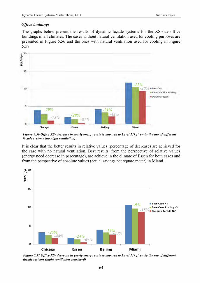
Dynamic Facade Systems- Master Thesis, LTH Sînziana Râșca
64
Office buildings
The graphs below present the results of dynamic façade systems for the XS-size office buildings in all climates. The cases without natural ventilation used for cooling purposes are presented in Figure 5.56 and the ones with natural ventilation used for cooling in Figure 5.57.
It is clear that the better results in relative values (percentage of decrease) are achieved for the case with no natural ventilation. Best results, from the perspective of relative values (energy need decrease in percentage), are achieve in the climate of Essen for both cases and from the perspective of absolute values (actual savings per square meter) in Miami.
Figure 5.56 Office XS- decrease in yearly energy costs (compared to Level 11) given by the use of different facade systems (no night ventilation)
-29% -29%
-21%
-11%
-75% -87% -48%
-20%
Figure 5.57 Office XS- decrease in yearly energy costs (compared to Level 11) given by the use of different facade systems (night ventilation considerd)
-25% -24%
-19%
-9%
-48% -69%
-33%
-18%
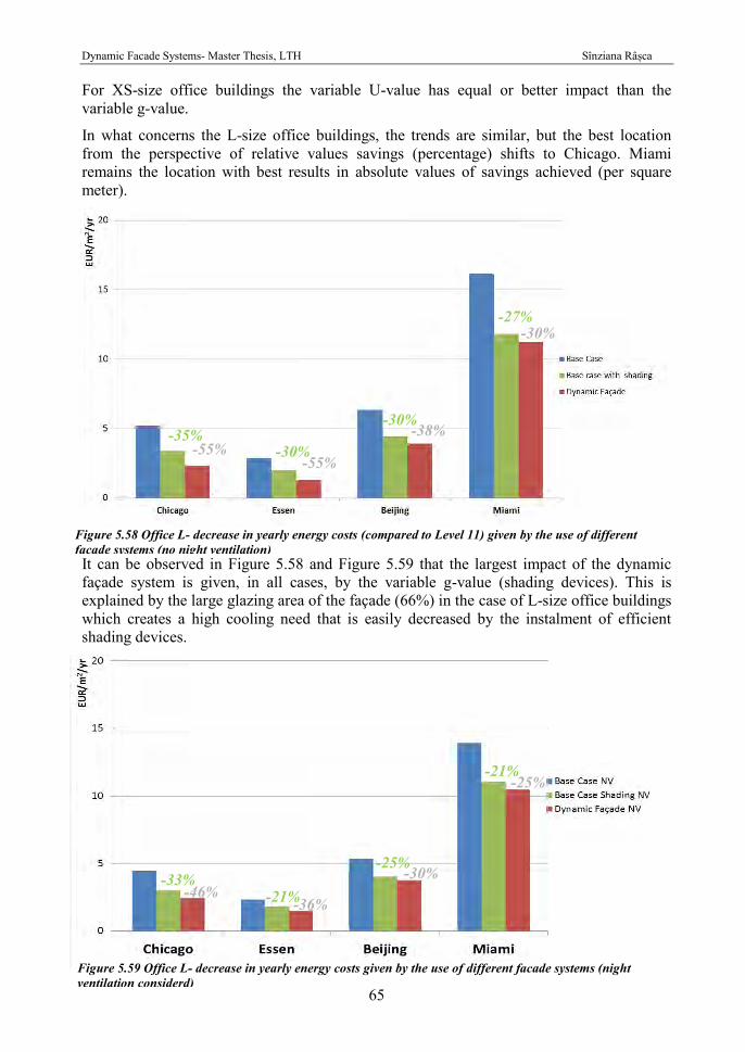
Dynamic Facade Systems- Master Thesis, LTH Sînziana Râșca
65
For XS-size office buildings the variable U-value has equal or better impact than the variable g-value.
In what concerns the L-size office buildings, the trends are similar, but the best location from the perspective of relative values savings (percentage) shifts to Chicago. Miami remains the location with best results in absolute values of savings achieved (per square meter).
It can be observed in Figure 5.58 and Figure 5.59 that the largest impact of the dynamic façade system is given, in all cases, by the variable g-value (shading devices). This is explained by the large glazing area of the façade (66%) in the case of L-size office buildings which creates a high cooling need that is easily decreased by the instalment of efficient shading devices.
Figure 5.58 Office L- decrease in yearly energy costs (compared to Level 11) given by the use of different facade systems (no night ventilation)
-35% -30%
-30%
-27%
-55% -55%
-38%
-30%
Figure 5.59 Office L- decrease in yearly energy costs given by the use of different facade systems (night ventilation considerd)
-33% -21%
-25%
-21%
-46% -36%
-30%
-25%

Dynamic Facade Systems- Master Thesis, LTH Sînziana Râșca
66
As mentioned before, when the natural ventilation for cooling purposes is activated, the impact of the dynamic façade system decreases visibly, mainly for the variable U-value.
Residential buildings In the case of the residential buildings, even though the trends remain similar, the impact is much smaller due to the different schedule of use. The fact that the buildings have the highest gains in the evening, and are occupied in the night reduces the efficiency of the dynamic facade. For the XS-size buildings, the largest reduction (percentage wise) is in Chicago for the case without natural ventilation (Figure 5.60) and in Miami for the case with natural ventilation (Figure 5.61), whilst savings wise Miami remains a constant as the location with the best results in both cases.
Figure 5.60 Residential XS- decrease in yearly energy costs (compared to Level 11) given by the use of different facade systems (no night ventilation)
-24% -21% -14%
-22%
-56% -54% -25%
-30%
-14% -19% -14%
-20%
-17% -21% -14%
-23%
Figure 5.61 Residential XS- decrease in yearly energy costs (compared to Level 11) given by the use of different facade systems (night ventilation considerd)
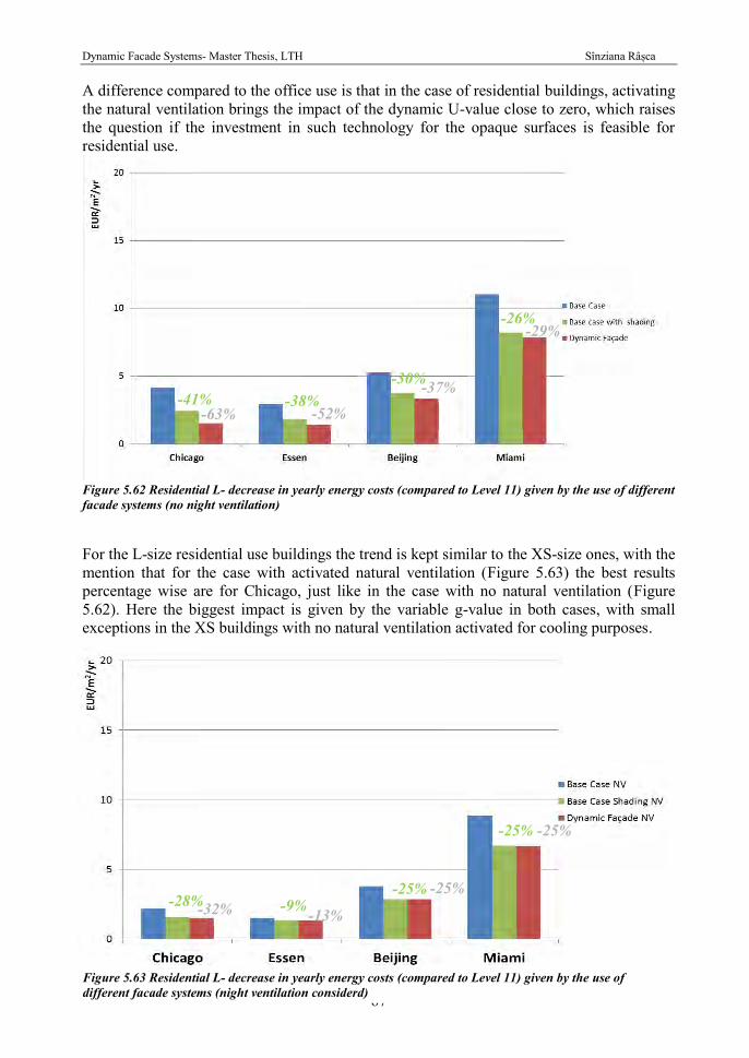
Dynamic Facade Systems- Master Thesis, LTH Sînziana Râșca
67
A difference compared to the office use is that in the case of residential buildings, activating the natural ventilation brings the impact of the dynamic U-value close to zero, which raises the question if the investment in such technology for the opaque surfaces is feasible for residential use.
Figure 5.62 Residential L- decrease in yearly energy costs (compared to Level 11) given by the use of different facade systems (no night ventilation)
For the L-size residential use buildings the trend is kept similar to the XS-size ones, with the mention that for the case with activated natural ventilation (Figure 5.63) the best results percentage wise are for Chicago, just like in the case with no natural ventilation (Figure 5.62). Here the biggest impact is given by the variable g-value in both cases, with small exceptions in the XS buildings with no natural ventilation activated for cooling purposes.
-41% -38% -30%
-26%
-63% -52% -37%
-29%
Figure 5.63 Residential L- decrease in yearly energy costs (compared to Level 11) given by the use of different facade systems (night ventilation considerd)
-28% -9% -25%
-25%
-32% -13%
-25%
-25%

Dynamic Facade Systems- Master Thesis, LTH Sînziana Râșca
68
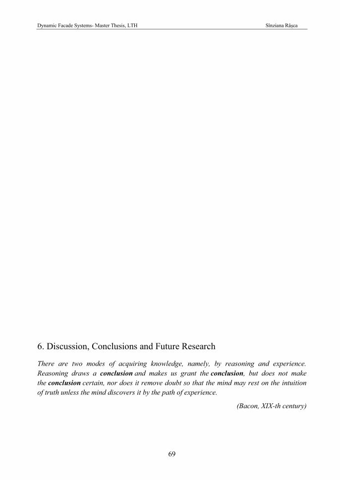
Dynamic Facade Systems- Master Thesis, LTH Sînziana Râșca
69
Discussion, Conclusions and Future Research 6.
There are two modes of acquiring knowledge, namely, by reasoning and experience. Reasoning draws a conclusion and makes us grant the conclusion, but does not make the conclusion certain, nor does it remove doubt so that the mind may rest on the intuition of truth unless the mind discovers it by the path of experience.
(Bacon, XIX-th century)
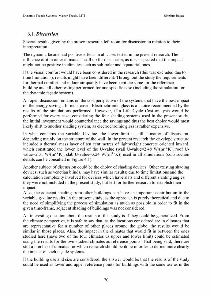
Dynamic Facade Systems- Master Thesis, LTH Sînziana Râșca
70
Discussion 6.1. Several results given by the present research left room for discussion in relation to their interpretation.
The dynamic facade had positive effects in all cases tested in the present research. The influence of it in other climates is still up for discussion, as it is suspected that the impact might not be positive in climates such as sub-polar and equatorial ones.
If the visual comfort would have been considered in the research (this was excluded due to time limitations), results might have been different. Throughout the study the requirements for thermal comfort and indoor air quality have been kept the same for the reference building and all other testing performed for one specific case (including the simulation for the dynamic façade system).
An open discussion remains on the cost perspective of the systems that have the best impact on the energy savings. In most cases, Electrochromic glass is a choice recommended by the results of the simulations performed. However, if a Life Cycle Cost analysis would be performed for every case, considering the four shading systems used in the present study, the initial investment would counterbalance the savings and thus the best choice would most likely shift to another shading system, as electrochromic glass is rather expensive.
In what concerns the variable U-value, the lower limit is still a matter of discussion, depending mainly on the structure of the wall. In the present research the envelope structure included a thermal mass layer of ten centimetres of lightweight concrete oriented inward, which constituted the lower level of the U-value (wall U-value=2.48 W/(m2*K), roof U-value=2.31 W/(m2*K), slab U-value=3.24 W/(m2*K)) used in all simulations (construction details can be consulted in Figure 4.1).
Another subject of discussion could be the choice of shading devices. Other existing shading devices, such as venetian blinds, may have similar results; due to time limitations and the calculation complexity involved for devices which have slats and different slanting angles, they were not included in the present study, but left for further research to establish their impact. Also, the adjacent shading from other buildings can have an important contribution to the variable g-value results. In the present study, as the approach is purely theoretical and due to the need of simplifying the process of simulation as much as possible in order to fit in the given time-frame, adjacent shading of buildings was not considered.
An interesting question about the results of this study is if they could be generalized. From the climate perspective, it is safe to say that, as the locations considered are in climates that are representative for a number of other places around the globe, the results would be similar in those places. Also, the impact in the climates that would fit in between the ones studied here (have two of the four climates us upper and lower limit) could be estimated using the results for the two studied climates as reference points. That being said, there are still a number of climates for which research should be done in order to define more clearly the impact of such façade systems.
If the building use and size are considered, the answer would be that the results of the study could be used as lower and upper reference points for buildings with the same use as in the
Dynamic Facade Systems- Master Thesis, LTH Sînziana Râșca
71
research, but sizes varying between 370 m2 (XS) and 6000 m2 (L) gross area. On the other hand, for different uses a new study would need to be undergone.
Conclusions 6.2. Considering the results presented in Chapter 5, the general conclusion can be drawn that the dynamic facade systems (variable U-value and variable g-value) have a positive impact on the overall energy demand of a building for all studied cases (if the reference is a building with passive house energy standard).
A second conclusion is that the impact of such a façade system on the overall energy use depends mainly on: the climate where the building is situated, the use of the building, the size of it and the use of natural ventilation for cooling purposes. The analysis show that, in the case where no natural ventilation is employed for cooling purposes, the energy need can have a decrease between 11% and 87% (as there is some uncertainty about the accuracy of the calculation, a variation +/- 10% for these results should be considered) compared to the passive house level (Passive House Institute, 2012), for office buildings situated in the climate with the best results. For residential use the impact varies between 14% and 63% in the same conditions. When natural ventilation is employed for cooling, the best results achieved are a decrease between 9% and 69% for the office use and between 9% and 32% for residential. Percentage wise, the best results are achieved for Essen and Chicago, as the climate for those locations permits the use of outdoor temperatures for cooling all year round. If analysed from the perspective of quantity, the most savings are achieved for Miami, as the amount of cooling need is much higher there and even though the percentage of savings is lower, it adds up to a better final result than all other locations.
In what concerns answering the question posed in the beginning of the study (stated in section 2.2), the system properties required to meet the best possible energy efficiency level are also dependant on the location, use and size of the building. The two system properties considered in the research, U-value and g-value, gave interesting results (presented in Chapter 4) in regard to their impact on the energy demand.
The question of the study (section 1.2), has been answered in the result section. The system properties of dynamic facades have been defined for each studied case with respect to the variable U-value and g-value.
For the U-value, an upper limit was establish with its value varying between 0.316 and 0.143W/( m2*K) for walls, 0.253 to 0.12 W/(m2*K) for roofs and 0.379 to 0.146 W/(m2*K) for slabs, according to location, use and size of the building.In what concerns the impact of the variable U-value for opaque elements of the envelope depending on a building’s use, the conclusion is that there is a much better impact for office buildings than for residential. Given the reduced savings for residential buildings, the investment in such an envelope technology might not be justified for residential use.
In respect to the U-value of the windows, the time limitations did not permit an in-depth study of this aspect. Still, a positive effect of such technology is proven by the testing of insulative shading devices (results can be followed in section 4.4). The conclusion in this case would be that older buildings with poor quality windows could have important benefits from the use of improved window systems with variable U-value.
The perspective on the variable g-value results is somewhat different than that over the U-values, as the optimum range for it is when the g-value can vary between 0% and 100%.
Dynamic Facade Systems- Master Thesis, LTH Sînziana Râșca
72
Therefore, the testing was done on four different shading devices with different properties and six different control systems. The conclusion here would be that if investment costs were overlooked and only the performance of the system considered, the best shading device for most cases would be Electrochromic glass, with a Solar activated control at 95W/m2, summer time only.
Depending on the climate, building use, size and age and window to wall ratio, the optimal shading and control system may vary. For older buildings an insulative shading device with Night Outside Temperature below 12oC and Day Cooling control would be optimal.
Looking at the results for the variable g-value in all locations, it is visible that in the case of Miami (and similar climates), mobile shading devices are not necessarily needed. This perspective reduces drastically the investment and maintenance costs if the right products are chosen.
As the final and more general conclusion of this research, it can be stated that Dynamic Façade Systems have most likely a positive impact on the energy demands of buildings in many climates around the world, but their impact varies according to a multitude of factors which need to be taken into account before deciding on employing such a system. Also, it is very important to control the system with the right settings according to the building’s locations, use and construction, so that maximum impact can be achieved. A thorough LCC analysis would be recommended before choosing a Dynamic Façade System.
Considering the results and the conclusions stated above, it can be stated that both the aim (section 1.2) and the set objectives (section 1.3) of the research have been met, but that there is still room for further research in the vast field of Dynamic Façade Systems.
Future Research 6.3. In such a new field of building technology as the Dynamic Façade Systems there is always plenty of room for “Future Research”. Probably some of the most important aspects that need to be approached in the future would be:
- The Impact of variable U-value for windows and the desired limits between which it should vary
- Further testing in different climates and building uses - Further testing for the impact of different shading devices and shading control
systems - The costs of such façade systems and their LCC compared with a static facade
in different situations - Technological perspective on the design of Dynamic Façade Systems - The possibility to develop highly transparent insulation materials that have
affordable prices.
Another point of open discussion is the possible effect of Dynamic Façade Systems on the thermal comfort of buildings. Even though stated as a point in the vision that drove the present project, it has been hard to study the impact such systems could have on the occupant’s comfort. The requirements set for the indoor climate have been kept the same throughout all simulations. This means that from the temperature and air quality perspective, the comfort requirements were met. It is left for further research to establish if any elements such as surface temperatures and condensation (which may appear on the inner surface of

Dynamic Facade Systems- Master Thesis, LTH Sînziana Râșca
73
the envelope due to the difference between inner surface temperature of the envelope and indoor air temperature) may cause discomfort to the users.
Dynamic Facade Systems- Master Thesis, LTH Sînziana Râșca
74
References 7.
No finite point has meaning without an infinite reference point.
(Jean-Paul Sartre)
Dynamic Facade Systems- Master Thesis, LTH Sînziana Râșca
75
1 Bosch,P, 2007, The Name of This Book Is Secret, Little, Brown Books for Young Readers, New York, 2007.
2 Butler,S., The Note-Books of Samuel Butler, Release Date: July, 2004 [EBook #6173] Edition: 10, http://www.gutenberg.org/dirs/etext04/nbsb10h.htm
3 Canadian Centre for Occupational Health and Safety, 2012, Space Requirements for Office Work, CCOHS, viewed 5 March 2014, http://www.ccohs.ca/oshanswers/ergonomics/office/working_space.html
4 Colombari, M, Kragh, M, Zobec, M, ”Introduction of Advanced Facade Technology”, 7th World Renewable Energy Congress; p. 634.
5 Control strategies for intelligent facades, S. Brandstrup, A. Valler 6 DIN V 18599-10:2011-12, 2011, Energy efficiency of buildings - Calculation of the net,
final and primary energy demand for heating, cooling, ventilation, domestic hot water and lighting - Part 10: Boundary conditions of use, climatic data, DIN, Germany.
7 DIRECTIVE 2002/91/EC, 2002, DIRECTIVE 2002/91/EC OF THE EUROPEAN PARLIAMENT AND OF THE COUNCIL OF THE EUROPEAN UNION 16 December 2002 on the energy performance of buildings, EUR-lex, viewed 15 February 2014, http://eur-lex.europa.eu/legal-content/EN/TXT/?uri=CELEX:32002L0091
8 EDSL, 2012, Tas Software, EDSL, viewed 22 February 2014, http://www.edsl.net/main/Software.aspx
9 Ekberg, L, 2007, “Revised Swedish Guidelines for the Specification of Indoor Climate”, Proceedings of Clima 2007 Wellbeing Indoors, pp.6
10 EnEV, 2004, Bekanntmachung der Neufassung der Energieeinsparverordnung (EnEV), EnEV-online, viewed 7 March 2014, http://www.enev-online.info/enev/enev_2004.pdf
11 Engineering Toolbox, 2014, Area per person, Engineering Toolbox, viewed 5 March 2014, http://www.engineeringtoolbox.com/number-persons-buildings-d_118.html
12 Eurostat, 2013, Electricity prices for household consumers, European Commission eurostat, viewed 13 February 2014, http://epp.eurostat.ec.europa.eu/tgm/table.do?tab=table&plugin=1&language=en&pcode=ten00115
13 FAO Corporate Document Repository, Mapping global urban and rural population distributions,viewed 10 February 2014, http://www.fao.org/docrep/009/a0310e/A0310E06.htm
14 G. Cellai, C. Carletti, F. Sciurpi and S. Secchi (2014), Transparent Building Envelope: Windows and Shading Devices Typologies for Energy Efficiency Refurbishments
15 G. Hausladen, P. Liedl, M. de Saldanha, 2012, Klimagerecht Bauen Ein Handbuch, Birkhauser, Basel, Switzerland
16 International Energy Agency IEA, 2014, Energy Efficiency, IEA, viewed 28 February 2014, http://www.iea.org/aboutus/faqs/energyefficiency/
17 ISO 15099, 2005, Thermal performance of windows, doors and shading devices -- Detailed calculations,International Organization for Standardisation, viewed 11 March 2014, http://www.iso.org/iso/catalogue_detail.htm?csnumber=26425
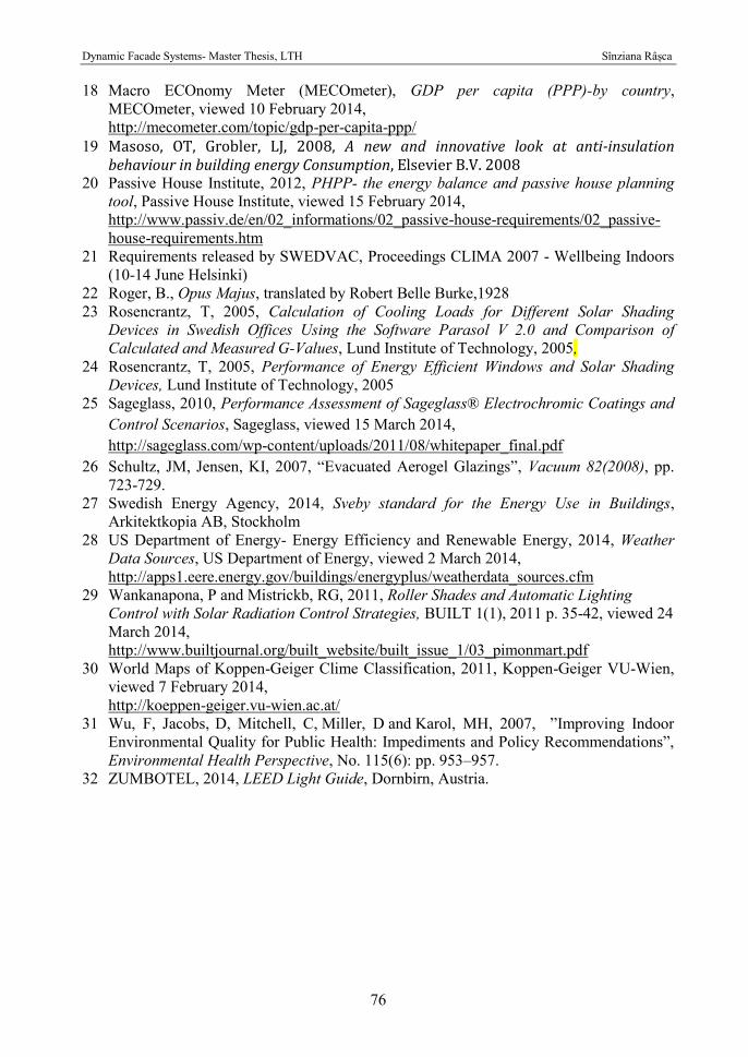
Dynamic Facade Systems- Master Thesis, LTH Sînziana Râșca
76
18 Macro ECOnomy Meter (MECOmeter), GDP per capita (PPP)-by country, MECOmeter, viewed 10 February 2014, http://mecometer.com/topic/gdp-per-capita-ppp/
19 Masoso, OT, Grobler, LJ, 2008, A new and innovative look at anti-insulation behaviour in building energy Consumption, Elsevier B.V. 2008
20 Passive House Institute, 2012, PHPP- the energy balance and passive house planning tool, Passive House Institute, viewed 15 February 2014, http://www.passiv.de/en/02_informations/02_passive-house-requirements/02_passive-house-requirements.htm
21 Requirements released by SWEDVAC, Proceedings CLIMA 2007 - Wellbeing Indoors (10-14 June Helsinki)
22 Roger, B., Opus Majus, translated by Robert Belle Burke,1928 23 Rosencrantz, T, 2005, Calculation of Cooling Loads for Different Solar Shading
Devices in Swedish Offices Using the Software Parasol V 2.0 and Comparison of Calculated and Measured G-Values, Lund Institute of Technology, 2005,
24 Rosencrantz, T, 2005, Performance of Energy Efficient Windows and Solar Shading Devices, Lund Institute of Technology, 2005
25 Sageglass, 2010, Performance Assessment of Sageglass® Electrochromic Coatings and Control Scenarios, Sageglass, viewed 15 March 2014, http://sageglass.com/wp-content/uploads/2011/08/whitepaper_final.pdf
26 Schultz, JM, Jensen, KI, 2007, “Evacuated Aerogel Glazings”, Vacuum 82(2008), pp. 723-729.
27 Swedish Energy Agency, 2014, Sveby standard for the Energy Use in Buildings, Arkitektkopia AB, Stockholm
28 US Department of Energy- Energy Efficiency and Renewable Energy, 2014, Weather Data Sources, US Department of Energy, viewed 2 March 2014, http://apps1.eere.energy.gov/buildings/energyplus/weatherdata_sources.cfm
29 Wankanapona, P and Mistrickb, RG, 2011, Roller Shades and Automatic Lighting Control with Solar Radiation Control Strategies, BUILT 1(1), 2011 p. 35-42, viewed 24 March 2014, http://www.builtjournal.org/built_website/built_issue_1/03_pimonmart.pdf
30 World Maps of Koppen-Geiger Clime Classification, 2011, Koppen-Geiger VU-Wien, viewed 7 February 2014, http://koeppen-geiger.vu-wien.ac.at/
31 Wu, F, Jacobs, D, Mitchell, C, Miller, D and Karol, MH, 2007, ”Improving Indoor Environmental Quality for Public Health: Impediments and Policy Recommendations”, Environmental Health Perspective, No. 115(6): pp. 953–957.
32 ZUMBOTEL, 2014, LEED Light Guide, Dornbirn, Austria.
Dynamic Facade Systems- Master Thesis, LTH Sînziana Râșca
77
Appendix 8.
“Appendix usually means "small outgrowth from large intestine," but in this case it means "additional information accompanying main text." Or are those really the same things? Think carefully before you insult this book.”
(Pseudonymous Bosch, 2007)
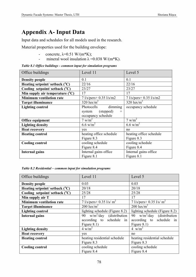
Dynamic Facade Systems- Master Thesis, LTH Sînziana Râșca
78
Appendix A- Input Data Input data and schedules for all models used in the research.
Material properties used for the building envelope:
- concrete, λ=0.51 W/(m*K); - mineral wool insulation λ =0.038 W/(m*K).
Table 8.1 Office buildings - common input for simulation programs
Office buildings Level 11 Level 5
Density people 0.1 0.1 Heating setpoint/ setback (oC) 22/16 22/16 Cooling setpoint/ setback (oC) 23/27 23/27 Min supply air temperature (oC) 17 17 Minimum ventilation rate 7 l/s/pers+ 0.35 l/s/m2 7 l/s/pers+ 0.35 l/s/m2 Target illuminance 320 lux/m2 320 lux/m2 Lighting control Photocells dimming
system (stepped) + occupancy schedule
occupancy schedule
Office equipment 7 w/m2 7 w/m2 Lighting density 6.6 w/m2 6.6 w/m2 Heat recovery yes no Heating control heating office schedule
Figure 8.3 heating office schedule Figure 8.3
Cooling control cooling schedule Figure 8.4
cooling schedule Figure 8.4
Internal gains Internal gains office Figure 8.1
Internal gains office Figure 8.1
Table 8.2 Residential – common input for simulation programs
Office buildings Level 11 Level 5
Density people 0.03 0.03 Heating setpoint/ setback (oC) 20/18 20/18 Cooling setpoint/ setback (oC) 25/28 25/28 Min supply air T 17 17 Minimum ventilation rate 7 l/s/pers+ 0.35 l/s/ m2 7 l/s/pers+ 0.35 l/s/ m2 Target illuminance 200 lux/m2 200 lux/m2 Lighting control lighting schedule (Figure 8.2) lighting schedule (Figure 8.2) Internal gains 90 w/m2/day (distribution
according to schedule in Figure 8.1)
90 w/m2/day (distribution according to schedule in Figure 8.1)
Lighting density 4 w/m2 4 w/m2 Heat recovery yes no Heating control heating residential schedule
Figure 8.3 heating residential schedule Figure 8.3
Cooling control cooling schedule Figure 8.4
cooling schedule Figure 8.4
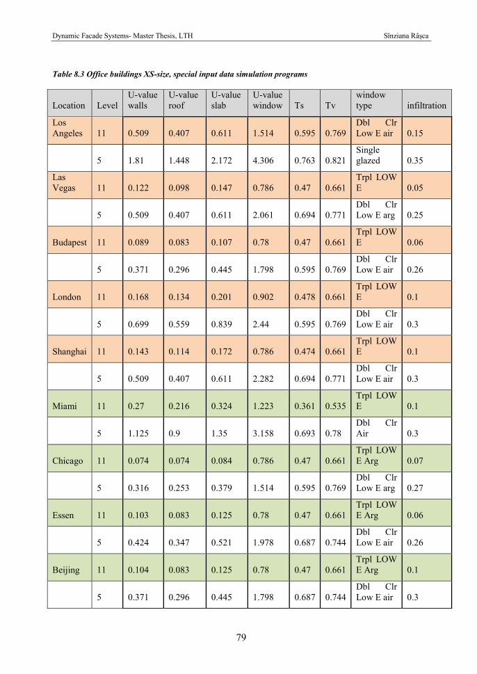
Dynamic Facade Systems- Master Thesis, LTH Sînziana Râșca
79
Table 8.3 Office buildings XS-size, special input data simulation programs
Location Level U-value walls
U-value roof
U-value slab
U-value window Ts Tv
window type infiltration
Los Angeles 11 0.509 0.407 0.611 1.514 0.595 0.769
Dbl Clr Low E air 0.15
5 1.81 1.448 2.172 4.306 0.763 0.821 Single glazed 0.35
Las Vegas 11 0.122 0.098 0.147 0.786 0.47 0.661
Trpl LOW E 0.05
5 0.509 0.407 0.611 2.061 0.694 0.771 Dbl Clr Low E arg 0.25
Budapest 11 0.089 0.083 0.107 0.78 0.47 0.661 Trpl LOW E 0.06
5 0.371 0.296 0.445 1.798 0.595 0.769 Dbl Clr Low E air 0.26
London 11 0.168 0.134 0.201 0.902 0.478 0.661 Trpl LOW E 0.1
5 0.699 0.559 0.839 2.44 0.595 0.769 Dbl Clr Low E air 0.3
Shanghai 11 0.143 0.114 0.172 0.786 0.474 0.661 Trpl LOW E 0.1
5 0.509 0.407 0.611 2.282 0.694 0.771 Dbl Clr Low E air 0.3
Miami 11 0.27 0.216 0.324 1.223 0.361 0.535 Trpl LOW E 0.1
5 1.125 0.9 1.35 3.158 0.693 0.78 Dbl Clr Air 0.3
Chicago 11 0.074 0.074 0.084 0.786 0.47 0.661 Trpl LOW E Arg 0.07
5 0.316 0.253 0.379 1.514 0.595 0.769 Dbl Clr Low E arg 0.27
Essen 11 0.103 0.083 0.125 0.78 0.47 0.661 Trpl LOW E Arg 0.06
5 0.424 0.347 0.521 1.978 0.687 0.744 Dbl Clr Low E air 0.26
Beijing 11 0.104 0.083 0.125 0.78 0.47 0.661 Trpl LOW E Arg 0.1
5 0.371 0.296 0.445 1.798 0.687 0.744 Dbl Clr Low E air 0.3
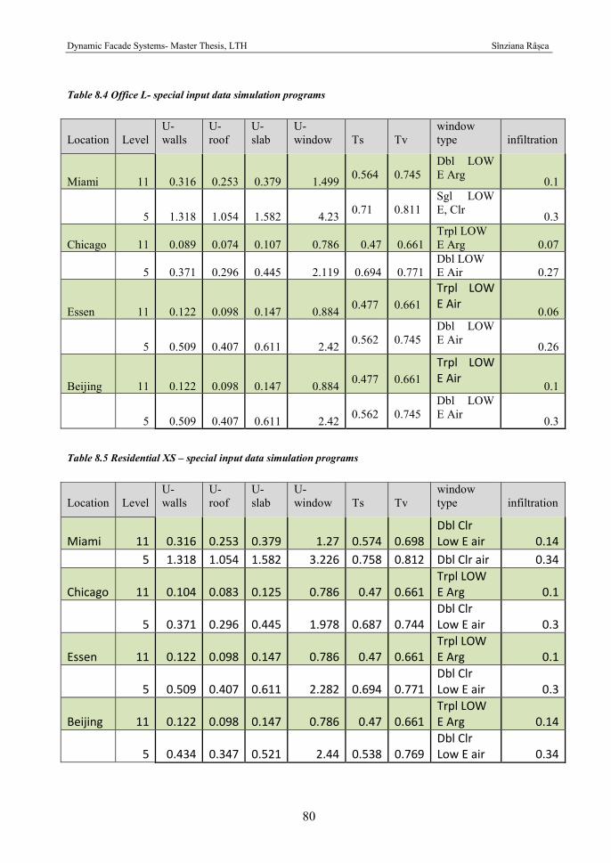
Dynamic Facade Systems- Master Thesis, LTH Sînziana Râșca
80
Table 8.4 Office L- special input data simulation programs
Table 8.5 Residential XS – special input data simulation programs
Location Level U-walls
U-roof
U-slab
U-window Ts Tv
window type infiltration
Miami 11 0.316 0.253 0.379 1.499 0.564 0.745 Dbl LOW E Arg 0.1
5 1.318 1.054 1.582 4.23 0.71 0.811 Sgl LOW E, Clr 0.3
Chicago 11 0.089 0.074 0.107 0.786 0.47 0.661 Trpl LOW E Arg 0.07
5 0.371 0.296 0.445 2.119 0.694 0.771 Dbl LOW E Air 0.27
Essen 11 0.122 0.098 0.147 0.884 0.477 0.661 Trpl LOW E Air
0.06
5 0.509 0.407 0.611 2.42 0.562 0.745 Dbl LOW E Air 0.26
Beijing 11 0.122 0.098 0.147 0.884 0.477 0.661 Trpl LOW E Air
0.1
5 0.509 0.407 0.611 2.42 0.562 0.745 Dbl LOW E Air 0.3
Location Level U-walls
U-roof
U-slab
U-window Ts Tv
window type infiltration
Miami 11 0.316 0.253 0.379 1.27 0.574 0.698 Dbl Clr Low E air 0.14
5 1.318 1.054 1.582 3.226 0.758 0.812 Dbl Clr air 0.34
Chicago 11 0.104 0.083 0.125 0.786 0.47 0.661 Trpl LOW E Arg 0.1
5 0.371 0.296 0.445 1.978 0.687 0.744 Dbl Clr Low E air 0.3
Essen 11 0.122 0.098 0.147 0.786 0.47 0.661 Trpl LOW E Arg 0.1
5 0.509 0.407 0.611 2.282 0.694 0.771 Dbl Clr Low E air 0.3
Beijing 11 0.122 0.098 0.147 0.786 0.47 0.661 Trpl LOW E Arg 0.14
5 0.434 0.347 0.521 2.44 0.538 0.769 Dbl Clr Low E air 0.34
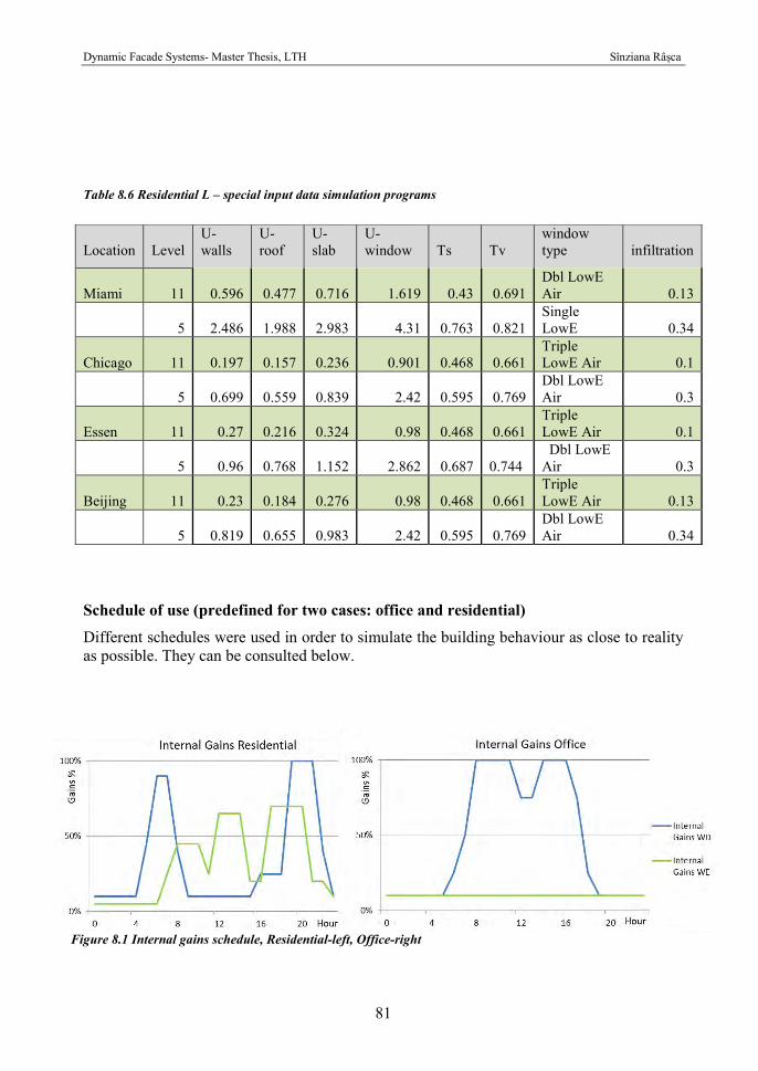
Dynamic Facade Systems- Master Thesis, LTH Sînziana Râșca
81
Table 8.6 Residential L – special input data simulation programs
Schedule of use (predefined for two cases: office and residential)
Different schedules were used in order to simulate the building behaviour as close to reality as possible. They can be consulted below.
Location Level U-walls
U-roof
U-slab
U-window Ts Tv
window type infiltration
Miami 11 0.596 0.477 0.716 1.619 0.43 0.691 Dbl LowE Air 0.13
5 2.486 1.988 2.983 4.31 0.763 0.821 Single LowE 0.34
Chicago 11 0.197 0.157 0.236 0.901 0.468 0.661 Triple LowE Air 0.1
5 0.699 0.559 0.839 2.42 0.595 0.769 Dbl LowE Air 0.3
Essen 11 0.27 0.216 0.324 0.98 0.468 0.661 Triple LowE Air 0.1
5 0.96 0.768 1.152 2.862 0.687 0.744 Dbl LowE Air 0.3
Beijing 11 0.23 0.184 0.276 0.98 0.468 0.661 Triple LowE Air 0.13
5 0.819 0.655 0.983 2.42 0.595 0.769 Dbl LowE Air 0.34
Figure 8.1 Internal gains schedule, Residential-left, Office-right
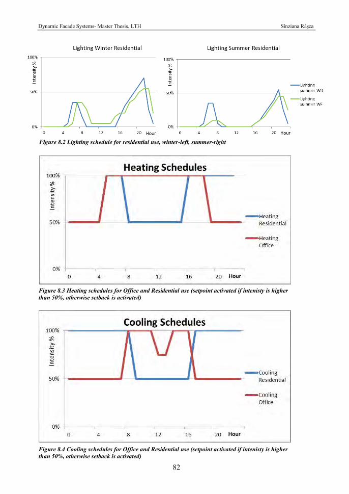
Dynamic Facade Systems- Master Thesis, LTH Sînziana Râșca
82
Figure 8.2 Lighting schedule for residential use, winter-left, summer-right
Figure 8.3 Heating schedules for Office and Residential use (setpoint activated if intenisty is higher than 50%, otherwise setback is activated)
Figure 8.4 Cooling schedules for Office and Residential use (setpoint activated if intenisty is higher than 50%, otherwise setback is activated)
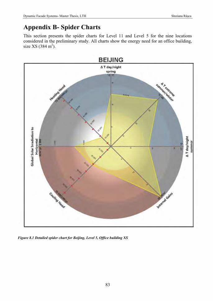
Dynamic Facade Systems- Master Thesis, LTH Sînziana Râșca
83
Appendix B- Spider Charts This section presents the spider charts for Level 11 and Level 5 for the nine locations considered in the preliminary study. All charts show the energy need for an office building, size XS (384 m2).
Figure 8.1 Detailed spider chart for Beijing, Level 5, Office building XS
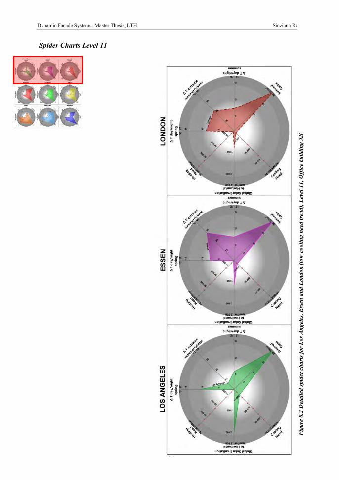
Dynamic Facade Systems- Master Thesis, LTH Sînziana Râșca
84
Spider Charts Level 11
Fig
ure
8.2
Det
aile
d sp
ider
cha
rts f
or L
os A
ngel
es, E
ssen
and
Lon
don
(low
coo
ling
need
tren
d), L
evel
11,
Off
ice
build
ing
XS
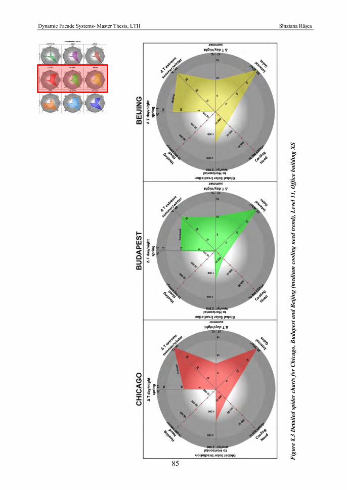
Dynamic Facade Systems- Master Thesis, LTH Sînziana Râșca
85
Fig
ure
8.3
Det
aile
d sp
ider
cha
rts f
or C
hica
go, B
udap
est a
nd B
eijin
g (m
ediu
m c
oolin
g ne
ed tr
end)
, Lev
el 1
1, O
ffic
e bu
ildin
g X
S
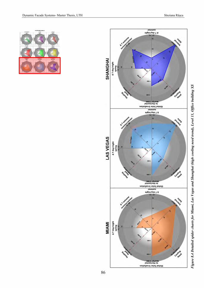
Dynamic Facade Systems- Master Thesis, LTH Sînziana Râșca
86
Fig
ure
8.4
Det
aile
d sp
ider
cha
rts f
or M
iam
i, La
s Veg
as a
nd S
hang
hai (
high
coo
ling
need
tren
d), L
evel
11,
Off
ice
build
ing
XS
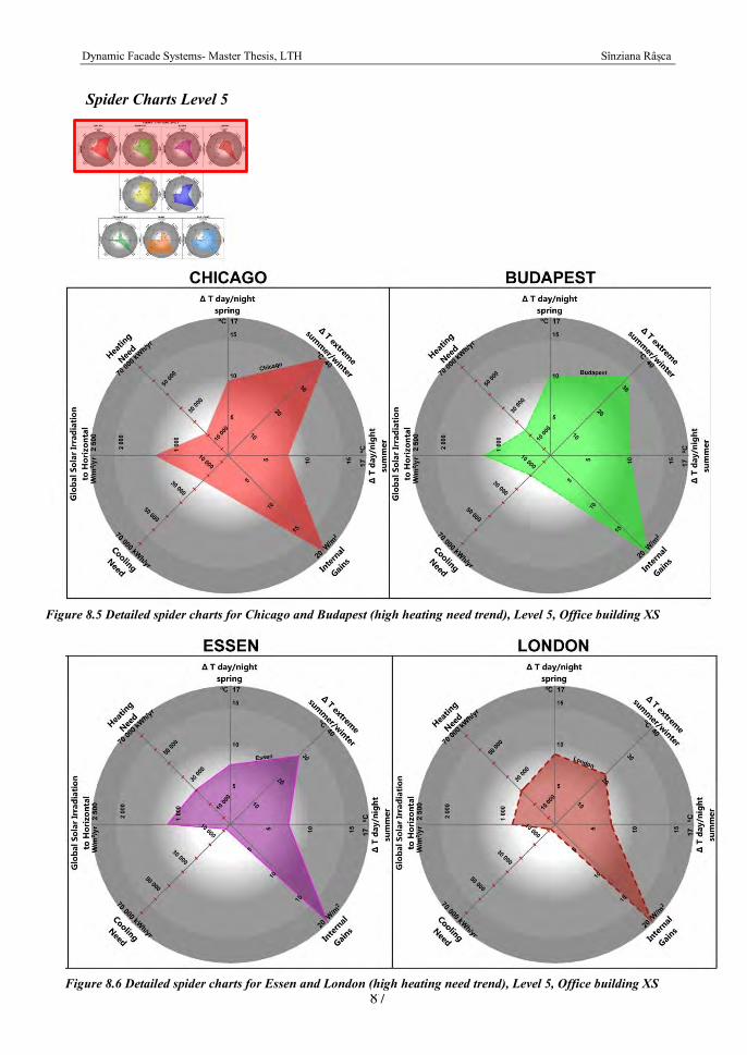
Dynamic Facade Systems- Master Thesis, LTH Sînziana Râșca
87
Spider Charts Level 5
Figure 8.5 Detailed spider charts for Chicago and Budapest (high heating need trend), Level 5, Office building XS
Figure 8.6 Detailed spider charts for Essen and London (high heating need trend), Level 5, Office building XS
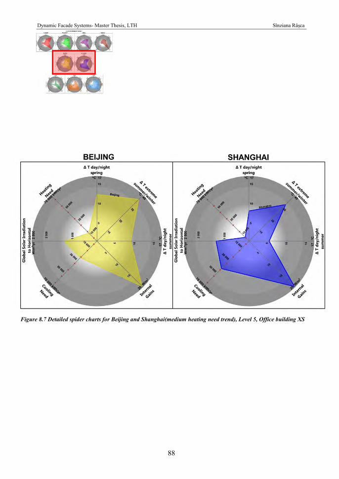
Dynamic Facade Systems- Master Thesis, LTH Sînziana Râșca
88
Figure 8.7 Detailed spider charts for Beijing and Shanghai(medium heating need trend), Level 5, Office building XS
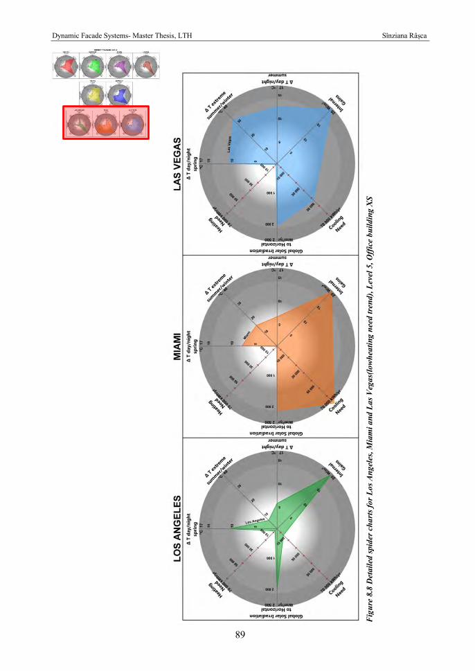
Dynamic Facade Systems- Master Thesis, LTH Sînziana Râșca
89
Fig
ure
8.8
Det
aile
d sp
ider
cha
rts f
or L
os A
ngel
es, M
iam
i and
Las
Veg
as(lo
whea
ting
need
tren
d), L
evel
5, O
ffic
e bu
ildin
g X
S
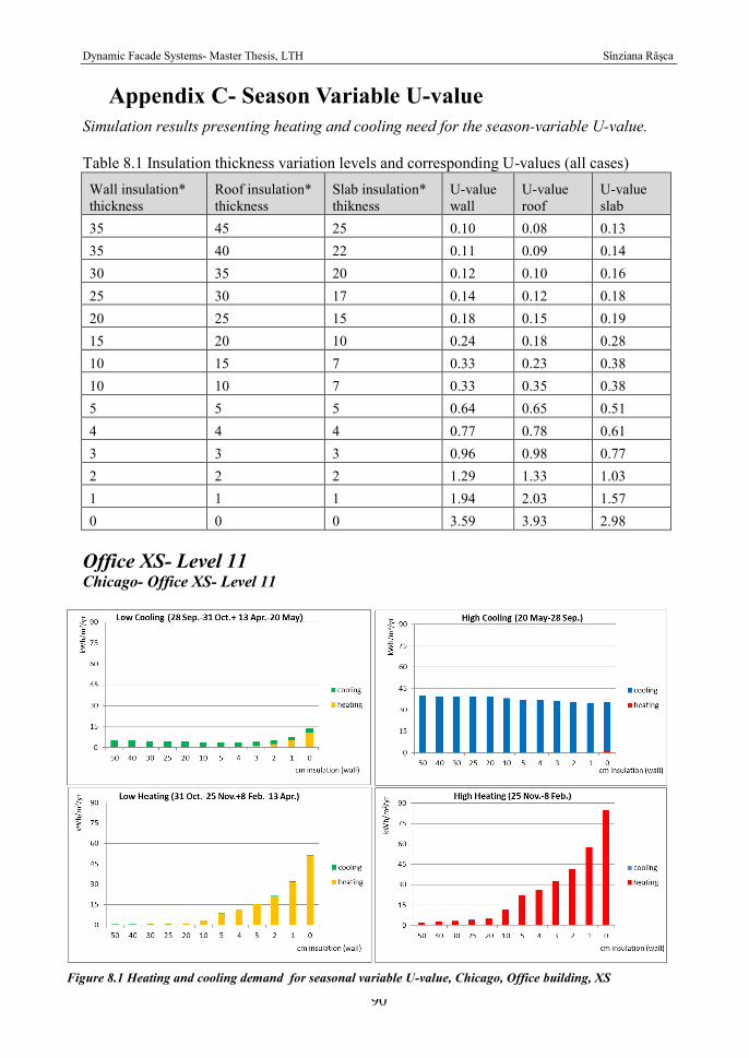
Dynamic Facade Systems- Master Thesis, LTH Sînziana Râșca
90
Appendix C- Season Variable U-value Simulation results presenting heating and cooling need for the season-variable U-value. Table 8.1 Insulation thickness variation levels and corresponding U-values (all cases) Wall insulation* thickness
Roof insulation* thickness
Slab insulation* thikness
U-value wall
U-value roof
U-value slab
35 45 25 0.10 0.08 0.13 35 40 22 0.11 0.09 0.14 30 35 20 0.12 0.10 0.16 25 30 17 0.14 0.12 0.18 20 25 15 0.18 0.15 0.19 15 20 10 0.24 0.18 0.28 10 15 7 0.33 0.23 0.38 10 10 7 0.33 0.35 0.38 5 5 5 0.64 0.65 0.51 4 4 4 0.77 0.78 0.61 3 3 3 0.96 0.98 0.77 2 2 2 1.29 1.33 1.03 1 1 1 1.94 2.03 1.57 0 0 0 3.59 3.93 2.98
Office XS- Level 11 Chicago- Office XS- Level 11
Figure 8.1 Heating and cooling demand for seasonal variable U-value, Chicago, Office building, XS
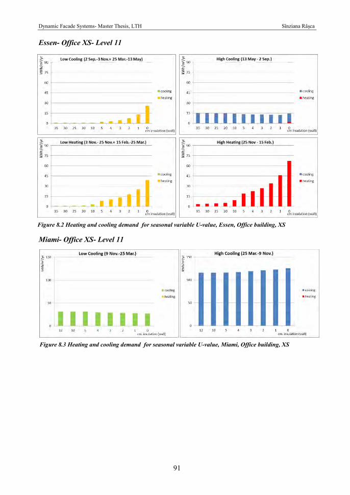
Dynamic Facade Systems- Master Thesis, LTH Sînziana Râșca
91
Essen- Office XS- Level 11
Miami- Office XS- Level 11
Figure 8.2 Heating and cooling demand for seasonal variable U-value, Essen, Office building, XS
Figure 8.3 Heating and cooling demand for seasonal variable U-value, Miami, Office building, XS
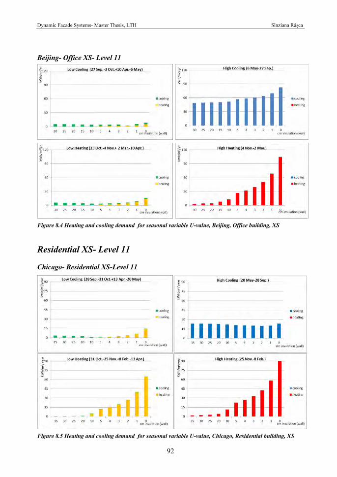
Dynamic Facade Systems- Master Thesis, LTH Sînziana Râșca
92
Beijing- Office XS- Level 11 Residential XS- Level 11 Chicago- Residential XS-Level 11
Figure 8.4 Heating and cooling demand for seasonal variable U-value, Beijing, Office building, XS
Figure 8.5 Heating and cooling demand for seasonal variable U-value, Chicago, Residential building, XS
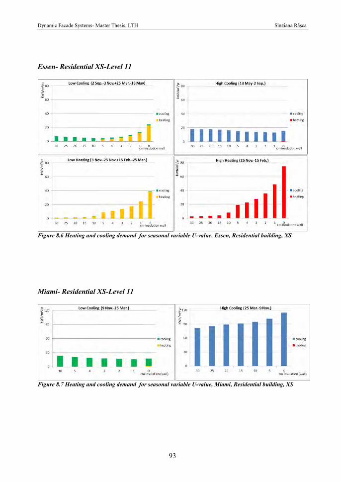
Dynamic Facade Systems- Master Thesis, LTH Sînziana Râșca
93
Essen- Residential XS-Level 11
Figure 8.6 Heating and cooling demand for seasonal variable U-value, Essen, Residential building, XS
Miami- Residential XS-Level 11
Figure 8.7 Heating and cooling demand for seasonal variable U-value, Miami, Residential building, XS
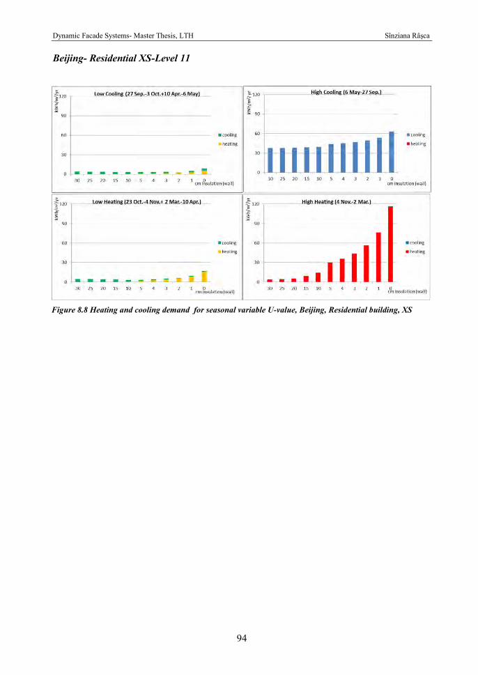
Dynamic Facade Systems- Master Thesis, LTH Sînziana Râșca
94
Beijing- Residential XS-Level 11
Figure 8.8 Heating and cooling demand for seasonal variable U-value, Beijing, Residential building, XS
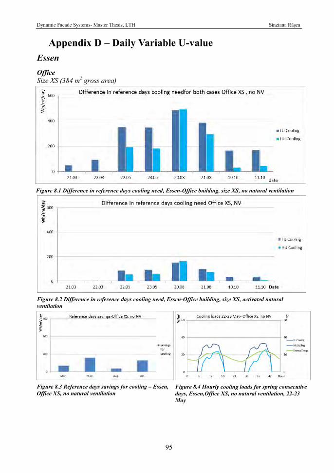
Dynamic Facade Systems- Master Thesis, LTH Sînziana Râșca
95
Appendix D – Daily Variable U-value Essen Office Size XS (384 m2 gross area)
Figure 8.1 Difference in reference days cooling need, Essen-Office building, size XS, no natural ventilation
Figure 8.2 Difference in reference days cooling need, Essen-Office building, size XS, activated natural ventilation
Figure 8.3 Reference days savings for cooling – Essen, Office XS, no natural ventilation
Figure 8.4 Hourly cooling loads for spring consecutive days, Essen,Office XS, no natural ventilation, 22-23 May
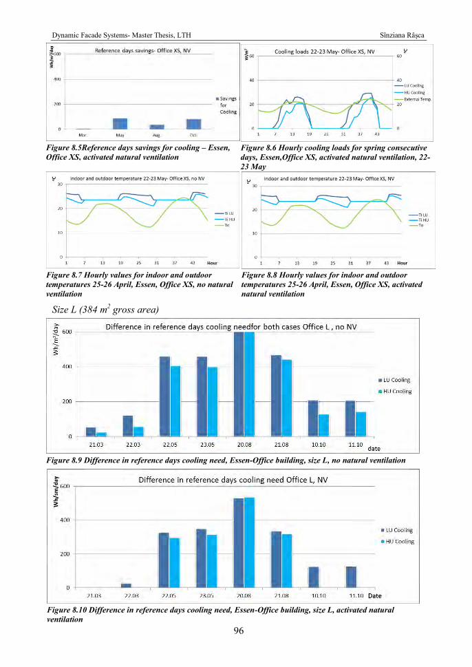
Dynamic Facade Systems- Master Thesis, LTH Sînziana Râșca
96
Size L (384 m2 gross area)
Figure 8.5Reference days savings for cooling – Essen, Office XS, activated natural ventilation
Figure 8.6 Hourly cooling loads for spring consecutive days, Essen,Office XS, activated natural ventilation, 22-23 May
Figure 8.7 Hourly values for indoor and outdoor temperatures 25-26 April, Essen, Office XS, no natural ventilation
Figure 8.8 Hourly values for indoor and outdoor temperatures 25-26 April, Essen, Office XS, activated natural ventilation
Figure 8.9 Difference in reference days cooling need, Essen-Office building, size L, no natural ventilation
Figure 8.10 Difference in reference days cooling need, Essen-Office building, size L, activated natural ventilation
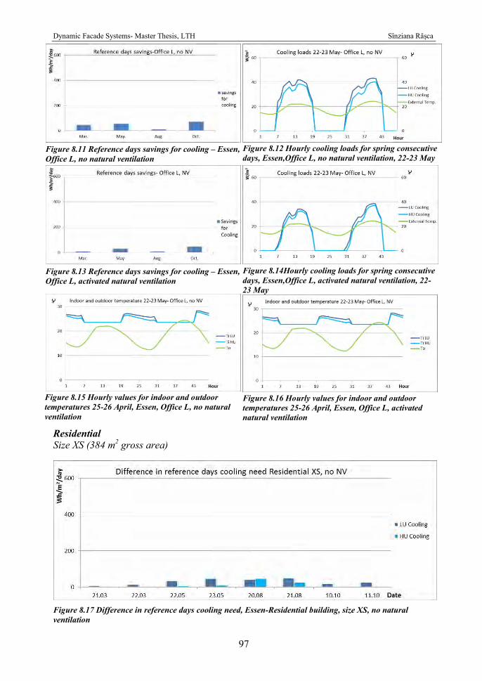
Dynamic Facade Systems- Master Thesis, LTH Sînziana Râșca
97
Residential Size XS (384 m2 gross area)
Figure 8.17 Difference in reference days cooling need, Essen-Residential building, size XS, no natural ventilation
Figure 8.11 Reference days savings for cooling – Essen, Office L, no natural ventilation
Figure 8.12 Hourly cooling loads for spring consecutive days, Essen,Office L, no natural ventilation, 22-23 May
Figure 8.14Hourly cooling loads for spring consecutive days, Essen,Office L, activated natural ventilation, 22-23 May
Figure 8.13 Reference days savings for cooling – Essen, Office L, activated natural ventilation
Figure 8.15 Hourly values for indoor and outdoor temperatures 25-26 April, Essen, Office L, no natural ventilation
Figure 8.16 Hourly values for indoor and outdoor temperatures 25-26 April, Essen, Office L, activated natural ventilation
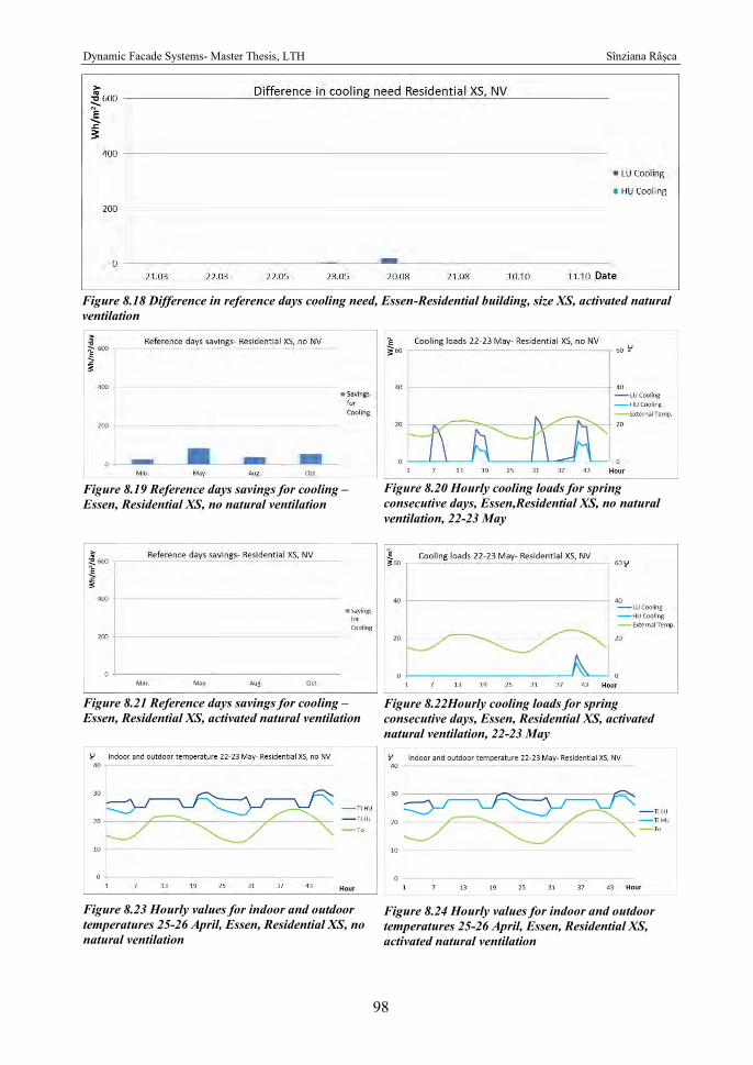
Dynamic Facade Systems- Master Thesis, LTH Sînziana Râșca
98
Figure 8.18 Difference in reference days cooling need, Essen-Residential building, size XS, activated natural ventilation
Figure 8.19 Reference days savings for cooling – Essen, Residential XS, no natural ventilation
Figure 8.21 Reference days savings for cooling – Essen, Residential XS, activated natural ventilation
Figure 8.20 Hourly cooling loads for spring consecutive days, Essen,Residential XS, no natural ventilation, 22-23 May
Figure 8.22Hourly cooling loads for spring consecutive days, Essen, Residential XS, activated natural ventilation, 22-23 May
Figure 8.23 Hourly values for indoor and outdoor temperatures 25-26 April, Essen, Residential XS, no natural ventilation
Figure 8.24 Hourly values for indoor and outdoor temperatures 25-26 April, Essen, Residential XS, activated natural ventilation
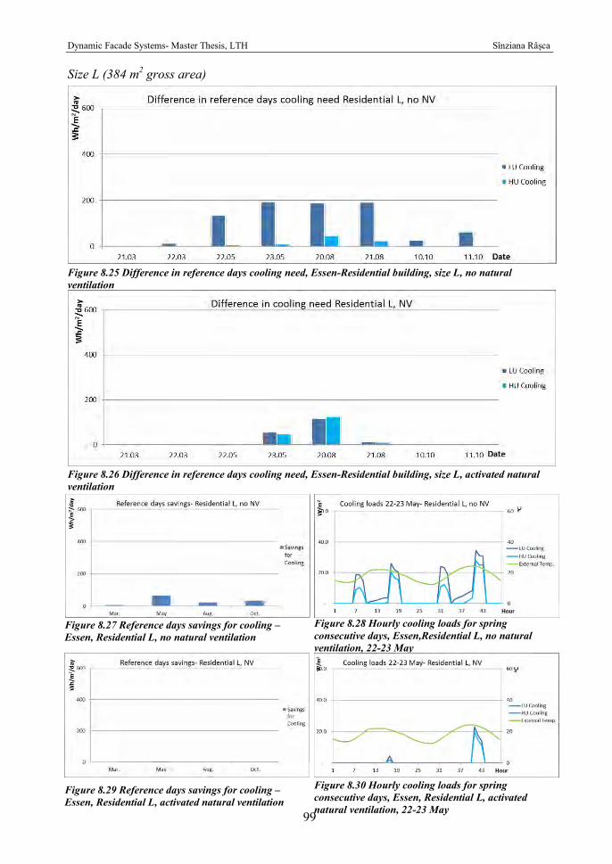
Dynamic Facade Systems- Master Thesis, LTH Sînziana Râșca
99
Size L (384 m2 gross area)
Figure 8.25 Difference in reference days cooling need, Essen-Residential building, size L, no natural ventilation
Figure 8.26 Difference in reference days cooling need, Essen-Residential building, size L, activated natural ventilation
Figure 8.27 Reference days savings for cooling – Essen, Residential L, no natural ventilation
Figure 8.28 Hourly cooling loads for spring consecutive days, Essen,Residential L, no natural ventilation, 22-23 May
Figure 8.29 Reference days savings for cooling – Essen, Residential L, activated natural ventilation
Figure 8.30 Hourly cooling loads for spring consecutive days, Essen, Residential L, activated natural ventilation, 22-23 May
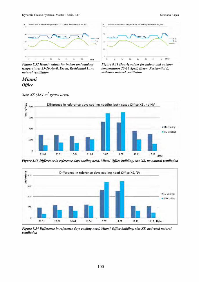
Dynamic Facade Systems- Master Thesis, LTH Sînziana Râșca
100
Miami Office Size XS (384 m2 gross area)
Figure 8.32 Hourly values for indoor and outdoor temperatures 25-26 April, Essen, Residential L, no natural ventilation
Figure 8.31 Hourly values for indoor and outdoor temperatures 25-26 April, Essen, Residential L, activated natural ventilation
Figure 8.33 Difference in reference days cooling need, Miami-Office building, size XS, no natural ventilation
Figure 8.34 Difference in reference days cooling need, Miami-Office building, size XS, activated natural ventilation
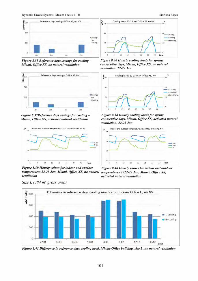
Dynamic Facade Systems- Master Thesis, LTH Sînziana Râșca
101
Size L (384 m2 gross area)
Figure 8.41 Difference in reference days cooling need, Miami-Office building, size L, no natural ventilation
Figure 8.35 Reference days savings for cooling – Miami, Office XS, no natural ventilation
Figure 8.37Reference days savings for cooling – Miami, Office XS, activated natural ventilation
Figure 8.36 Hourly cooling loads for spring consecutive days, Miami, Office XS, no natural ventilation, 22-23 Jan
Figure 8.38 Hourly cooling loads for spring consecutive days, Miami, Office XS, activated natural ventilation, 22-23 Jan
Figure 8.39 Hourly values for indoor and outdoor temperatures 22-23 Jan, Miami, Office XS, no natural ventilation
Figure 8.40 Hourly values for indoor and outdoor temperatures 2522-23 Jan, Miami, Office XS, activated natural ventilation
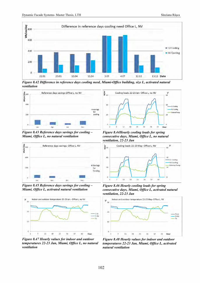
Dynamic Facade Systems- Master Thesis, LTH Sînziana Râșca
102
Figure 8.42 Difference in reference days cooling need, Miami-Office building, size L, activated natural ventilation
Figure 8.43 Reference days savings for cooling – Miami, Office L, no natural ventilation
Figure 8.45 Reference days savings for cooling – Miami, Office L, activated natural ventilation
Figure 8.44Hourly cooling loads for spring consecutive days, Miami, Office L, no natural ventilation, 22-23 Jan
Figure 8.46 Hourly cooling loads for spring consecutive days, Miami, Office L, activated natural ventilation, 22-23 Jan
Figure 8.47 Hourly values for indoor and outdoor temperatures 22-23 Jan, Miami, Office L, no natural ventilation
Figure 8.48 Hourly values for indoor and outdoor temperatures 22-23 Jan, Miami, Office L, activated natural ventilation
Dynamic Facade Systems- Master Thesis, LTH Sînziana Râșca
103
Residential Size XS (384 m2 gross area)
Figure 8.49 Difference in reference days cooling need, Miami-Residential building, size XS, no natural ventilation
Figure 8.50 Difference in reference days cooling need, Miami-Residential building, size XS, activated natural ventilation
Figure 8.51 Reference days savings for cooling – Miami, Residential XS, no natural ventilation
Figure 8.53 Reference days savings for cooling – Miami, Residential XS, activated natural ventilation
Figure 8.52Hourly cooling loads for spring consecutive days, Miami, Residential XS, no natural ventilation, 22-23 Jan
Figure 8.54 Hourly cooling loads for spring consecutive days, Miami, Residential XS, activated natural ventilation, 22-23 Jan
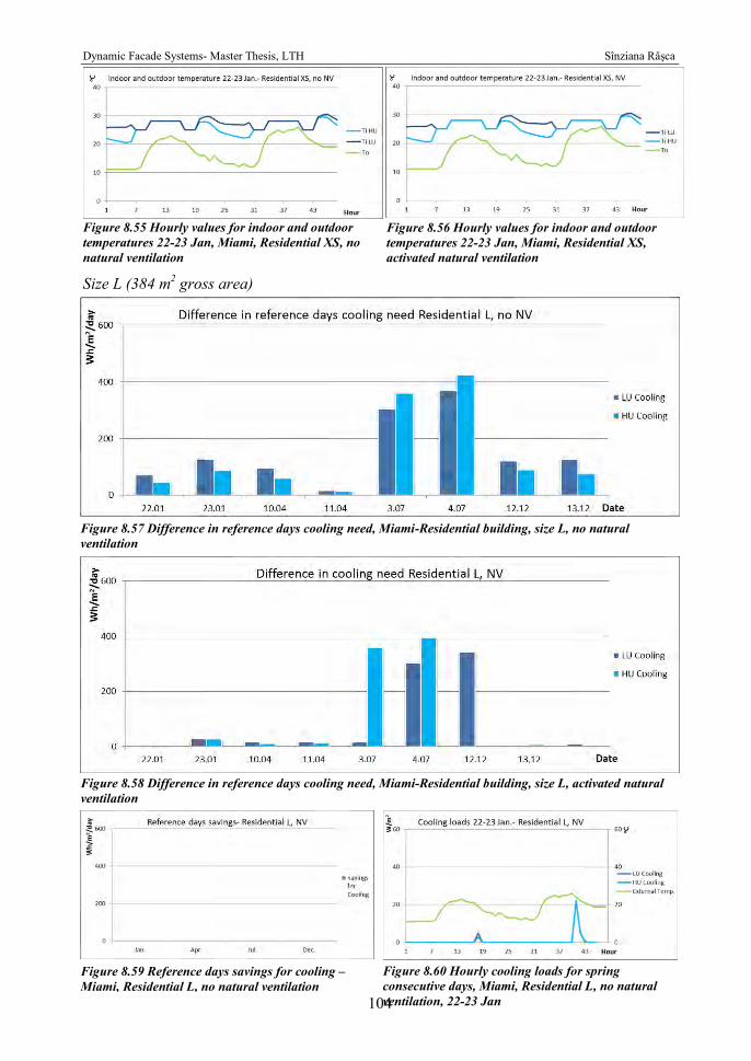
Dynamic Facade Systems- Master Thesis, LTH Sînziana Râșca
104
Size L (384 m2 gross area)
Figure 8.57 Difference in reference days cooling need, Miami-Residential building, size L, no natural ventilation
Figure 8.58 Difference in reference days cooling need, Miami-Residential building, size L, activated natural ventilation
Figure 8.59 Reference days savings for cooling – Miami, Residential L, no natural ventilation
Figure 8.60 Hourly cooling loads for spring consecutive days, Miami, Residential L, no natural ventilation, 22-23 Jan
Figure 8.55 Hourly values for indoor and outdoor temperatures 22-23 Jan, Miami, Residential XS, no natural ventilation
Figure 8.56 Hourly values for indoor and outdoor temperatures 22-23 Jan, Miami, Residential XS, activated natural ventilation
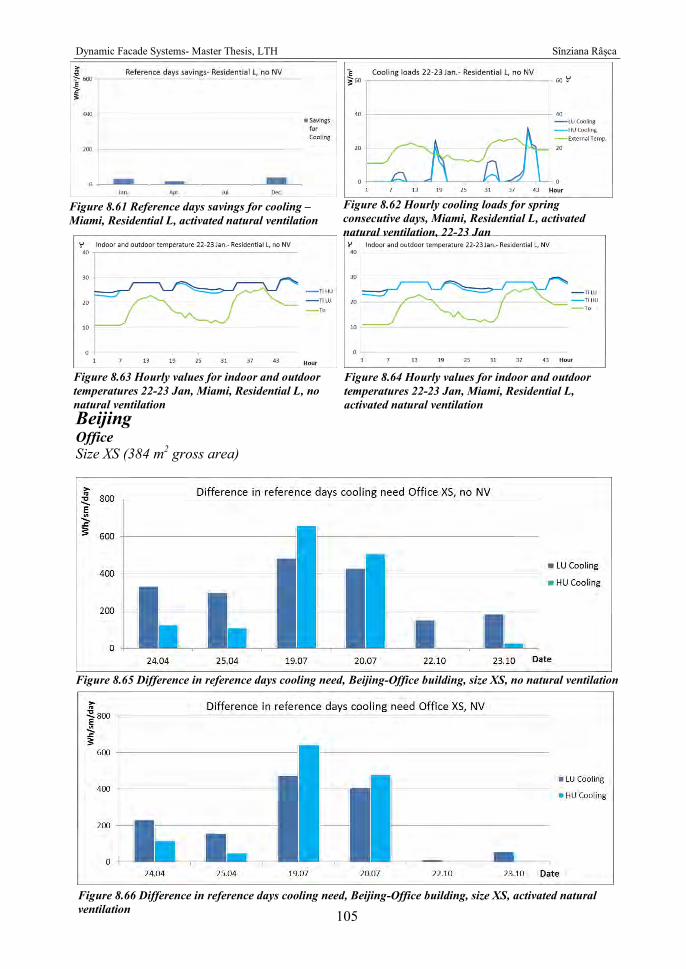
Dynamic Facade Systems- Master Thesis, LTH Sînziana Râșca
105
Beijing Office Size XS (384 m2 gross area)
Figure 8.61 Reference days savings for cooling – Miami, Residential L, activated natural ventilation
Figure 8.62 Hourly cooling loads for spring consecutive days, Miami, Residential L, activated natural ventilation, 22-23 Jan
Figure 8.63 Hourly values for indoor and outdoor temperatures 22-23 Jan, Miami, Residential L, no natural ventilation
Figure 8.64 Hourly values for indoor and outdoor temperatures 22-23 Jan, Miami, Residential L, activated natural ventilation
Figure 8.65 Difference in reference days cooling need, Beijing-Office building, size XS, no natural ventilation
Figure 8.66 Difference in reference days cooling need, Beijing-Office building, size XS, activated natural ventilation
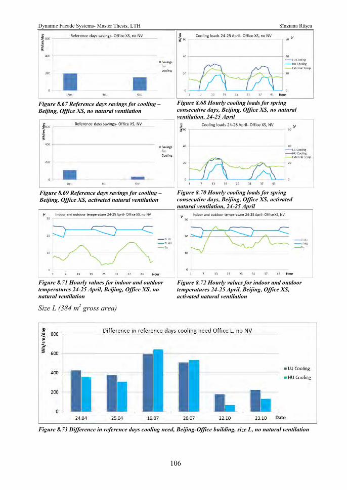
Dynamic Facade Systems- Master Thesis, LTH Sînziana Râșca
106
Size L (384 m2 gross area)
Figure 8.73 Difference in reference days cooling need, Beijing-Office building, size L, no natural ventilation
Figure 8.67 Reference days savings for cooling – Beijing, Office XS, no natural ventilation
Figure 8.69 Reference days savings for cooling – Beijing, Office XS, activated natural ventilation
Figure 8.68 Hourly cooling loads for spring consecutive days, Beijing, Office XS, no natural ventilation, 24-25 April
Figure 8.70 Hourly cooling loads for spring consecutive days, Beijing, Office XS, activated natural ventilation, 24-25 April
Figure 8.71 Hourly values for indoor and outdoor temperatures 24-25 April, Beijing, Office XS, no natural ventilation
Figure 8.72 Hourly values for indoor and outdoor temperatures 24-25 April, Beijing, Office XS, activated natural ventilation
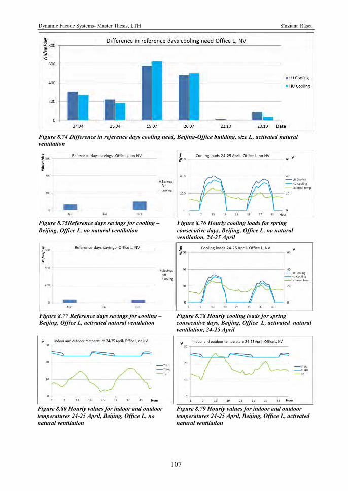
Dynamic Facade Systems- Master Thesis, LTH Sînziana Râșca
107
Figure 8.74 Difference in reference days cooling need, Beijing-Office building, size L, activated natural ventilation
Figure 8.75Reference days savings for cooling – Beijing, Office L, no natural ventilation
Figure 8.77 Reference days savings for cooling – Beijing, Office L, activated natural ventilation
Figure 8.76 Hourly cooling loads for spring consecutive days, Beijing, Office L, no natural ventilation, 24-25 April
Figure 8.78 Hourly cooling loads for spring consecutive days, Beijing, Office L, activated natural ventilation, 24-25 April
Figure 8.80 Hourly values for indoor and outdoor temperatures 24-25 April, Beijing, Office L, no natural ventilation
Figure 8.79 Hourly values for indoor and outdoor temperatures 24-25 April, Beijing, Office L, activated natural ventilation
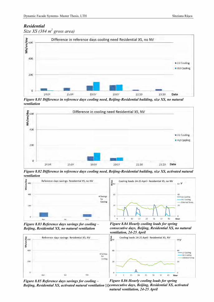
Dynamic Facade Systems- Master Thesis, LTH Sînziana Râșca
108
Residential Size XS (384 m2 gross area)
Figure 8.81 Difference in reference days cooling need, Beijing-Residential building, size XS, no natural ventilation
Figure 8.82 Difference in reference days cooling need, Beijing-Residential building, size XS, activated natural ventilation
Figure 8.83 Reference days savings for cooling – Beijing, Residential XS, no natural ventilation
Figure 8.85 Reference days savings for cooling – Beijing, Residential XS, activated natural ventilation
Figure 8.84 Hourly cooling loads for spring consecutive days, Beijing, Residential XS, no natural ventilation, 24-25 April
Figure 8.86 Hourly cooling loads for spring consecutive days, Beijing, Residential XS, activated natural ventilation, 24-25 April
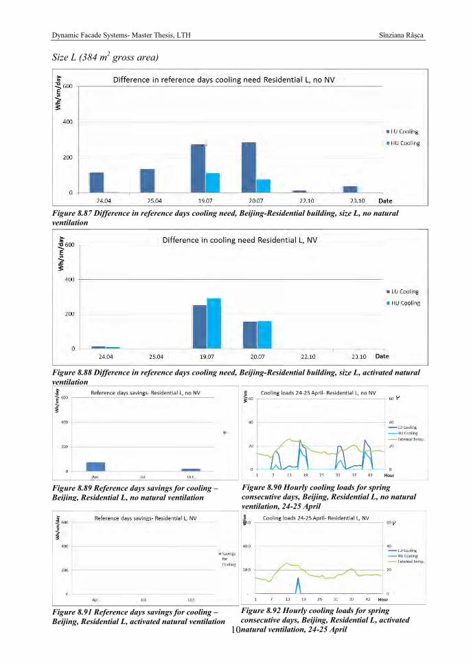
Dynamic Facade Systems- Master Thesis, LTH Sînziana Râșca
109
Size L (384 m2 gross area)
Figure 8.88 Difference in reference days cooling need, Beijing-Residential building, size L, activated natural ventilation
Figure 8.87 Difference in reference days cooling need, Beijing-Residential building, size L, no natural ventilation
Figure 8.89 Reference days savings for cooling – Beijing, Residential L, no natural ventilation
Figure 8.91 Reference days savings for cooling – Beijing, Residential L, activated natural ventilation
Figure 8.90 Hourly cooling loads for spring consecutive days, Beijing, Residential L, no natural ventilation, 24-25 April
Figure 8.92 Hourly cooling loads for spring consecutive days, Beijing, Residential L, activated natural ventilation, 24-25 April
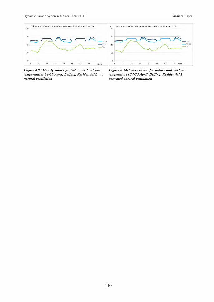
Dynamic Facade Systems- Master Thesis, LTH Sînziana Râșca
110
Figure 8.94Hourly values for indoor and outdoor temperatures 24-25 April, Beijing, Residential L, activated natural ventilation
Figure 8.93 Hourly values for indoor and outdoor temperatures 24-25 April, Beijing, Residential L, no natural ventilation
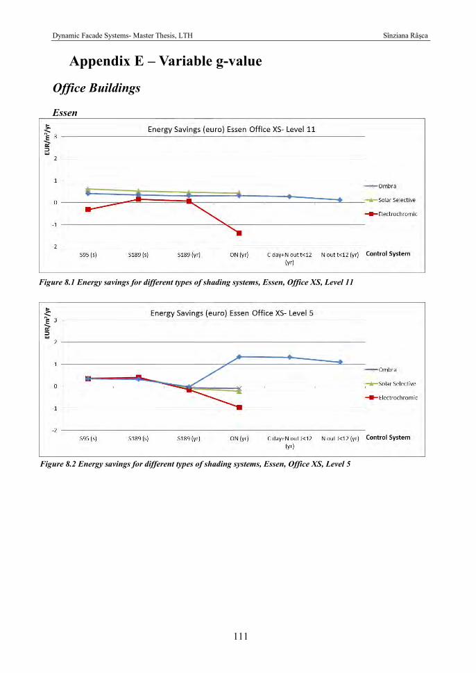
Dynamic Facade Systems- Master Thesis, LTH Sînziana Râșca
111
Appendix E – Variable g-value
Office Buildings Essen
Figure 8.1 Energy savings for different types of shading systems, Essen, Office XS, Level 11
Figure 8.2 Energy savings for different types of shading systems, Essen, Office XS, Level 5
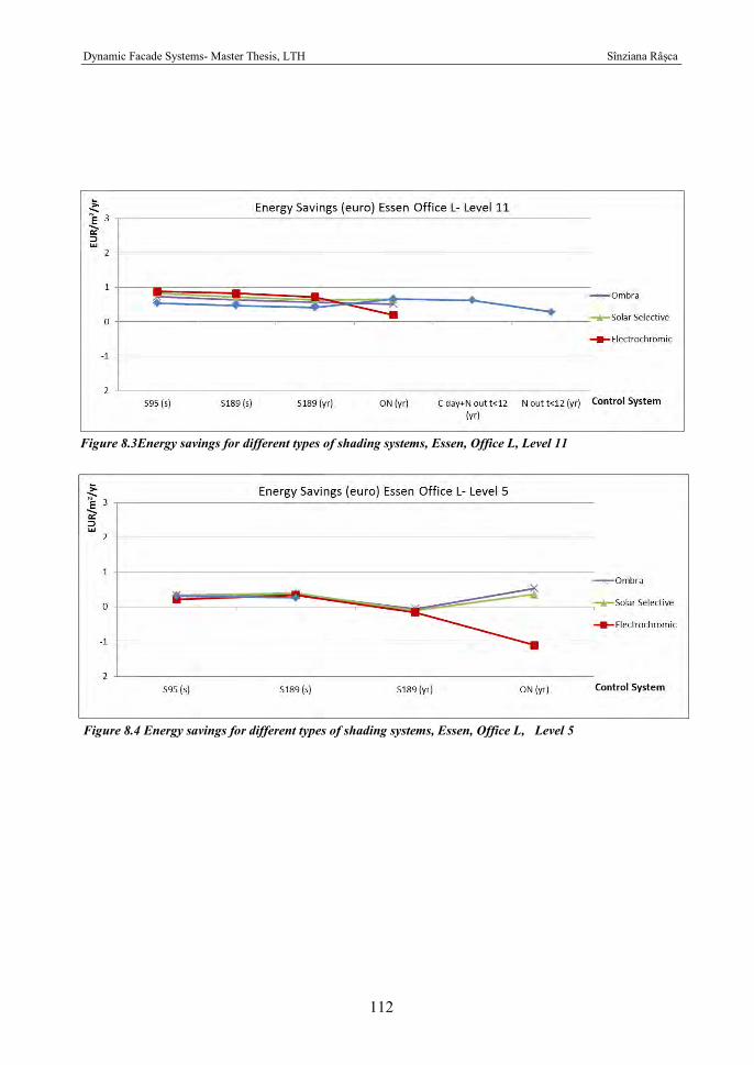
Dynamic Facade Systems- Master Thesis, LTH Sînziana Râșca
112
Figure 8.3Energy savings for different types of shading systems, Essen, Office L, Level 11
Figure 8.4 Energy savings for different types of shading systems, Essen, Office L, Level 5
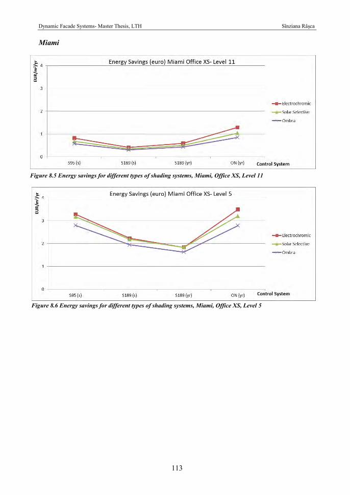
Dynamic Facade Systems- Master Thesis, LTH Sînziana Râșca
113
Miami
Figure 8.5 Energy savings for different types of shading systems, Miami, Office XS, Level 11
Figure 8.6 Energy savings for different types of shading systems, Miami, Office XS, Level 5
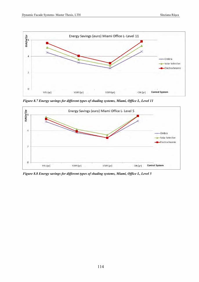
Dynamic Facade Systems- Master Thesis, LTH Sînziana Râșca
114
Figure 8.7 Energy savings for different types of shading systems, Miami, Office L, Level 11
Figure 8.8 Energy savings for different types of shading systems, Miami, Office L, Level 5
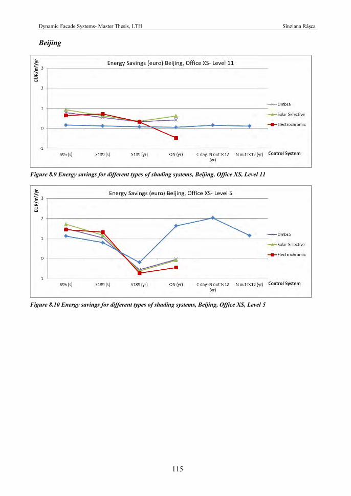
Dynamic Facade Systems- Master Thesis, LTH Sînziana Râșca
115
Beijing
Figure 8.9 Energy savings for different types of shading systems, Beijing, Office XS, Level 11
Figure 8.10 Energy savings for different types of shading systems, Beijing, Office XS, Level 5
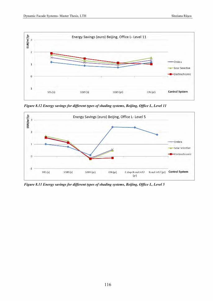
Dynamic Facade Systems- Master Thesis, LTH Sînziana Râșca
116
Figure 8.12 Energy savings for different types of shading systems, Beijing, Office L, Level 11
Figure 8.11 Energy savings for different types of shading systems, Beijing, Office L, Level 5
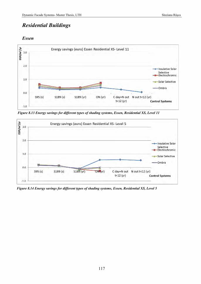
Dynamic Facade Systems- Master Thesis, LTH Sînziana Râșca
117
Residential Buildings
Essen
Figure 8.13 Energy savings for different types of shading systems, Essen, Residential XS, Level 11
Figure 8.14 Energy savings for different types of shading systems, Essen, Residential XS, Level 5
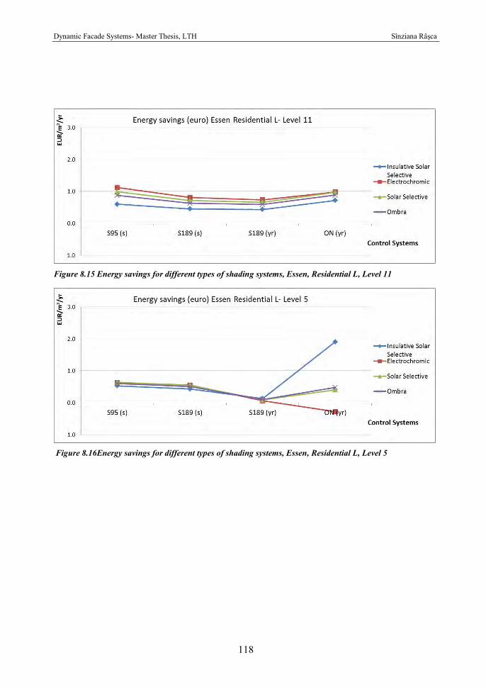
Dynamic Facade Systems- Master Thesis, LTH Sînziana Râșca
118
Figure 8.15 Energy savings for different types of shading systems, Essen, Residential L, Level 11
Figure 8.16Energy savings for different types of shading systems, Essen, Residential L, Level 5
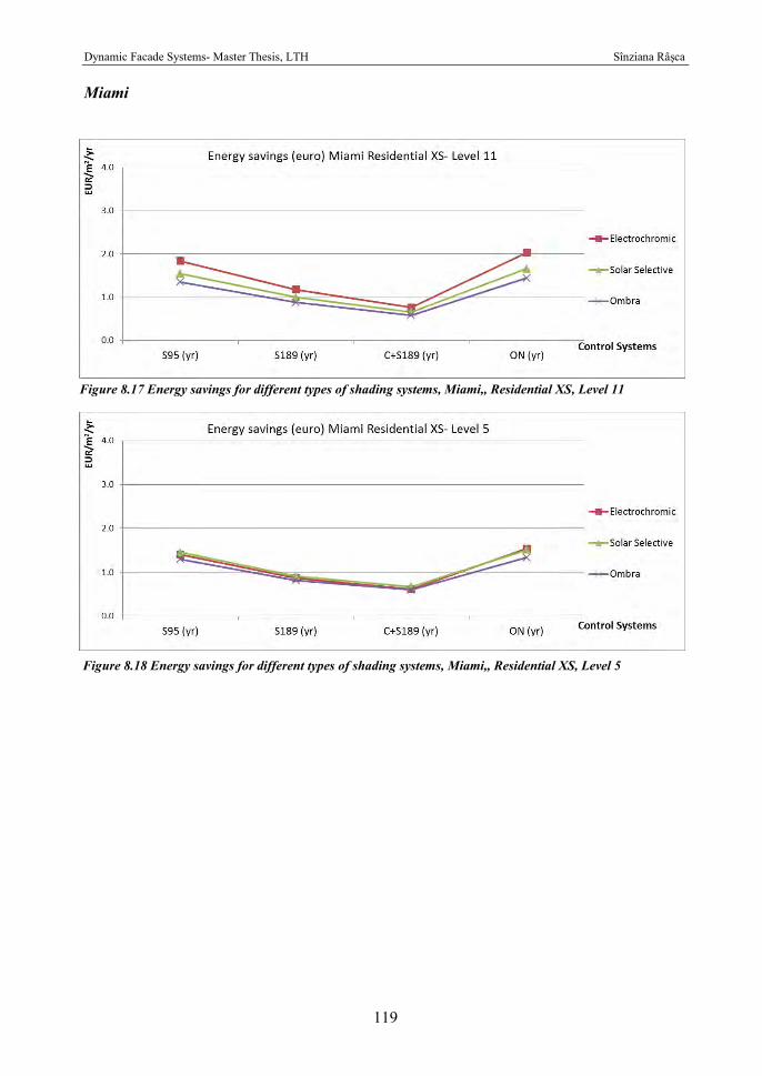
Dynamic Facade Systems- Master Thesis, LTH Sînziana Râșca
119
Miami
Figure 8.17 Energy savings for different types of shading systems, Miami,, Residential XS, Level 11
Figure 8.18 Energy savings for different types of shading systems, Miami,, Residential XS, Level 5
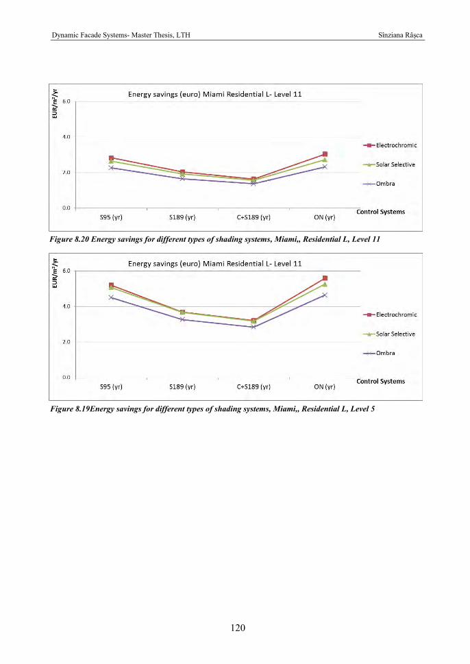
Dynamic Facade Systems- Master Thesis, LTH Sînziana Râșca
120
Figure 8.20 Energy savings for different types of shading systems, Miami,, Residential L, Level 11
Figure 8.19Energy savings for different types of shading systems, Miami,, Residential L, Level 5
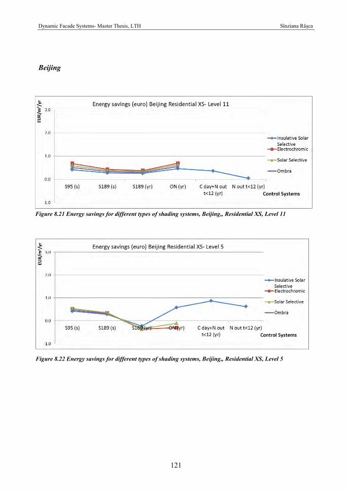
Dynamic Facade Systems- Master Thesis, LTH Sînziana Râșca
121
Beijing
Figure 8.21 Energy savings for different types of shading systems, Beijing,, Residential XS, Level 11
Figure 8.22 Energy savings for different types of shading systems, Beijing,, Residential XS, Level 5
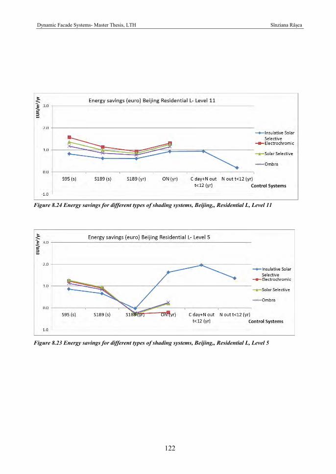
Dynamic Facade Systems- Master Thesis, LTH Sînziana Râșca
122
Figure 8.24 Energy savings for different types of shading systems, Beijing,, Residential L, Level 11
Figure 8.23 Energy savings for different types of shading systems, Beijing,, Residential L, Level 5
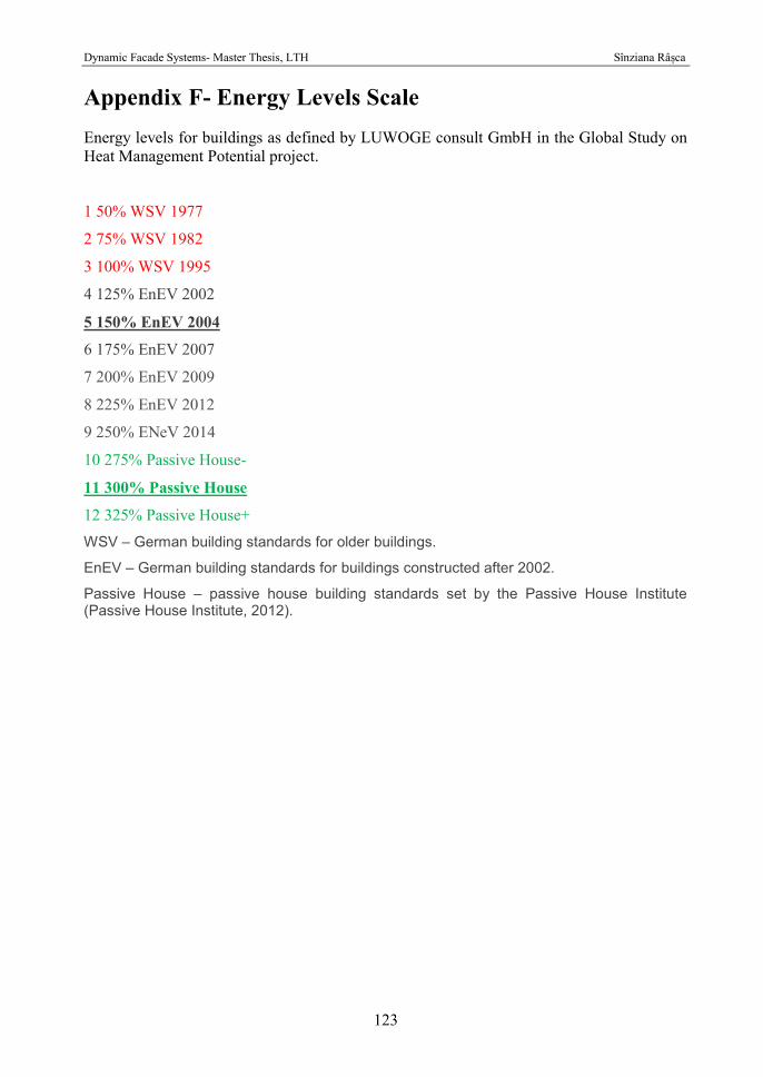
Dynamic Facade Systems- Master Thesis, LTH Sînziana Râșca
123
Appendix F- Energy Levels Scale Energy levels for buildings as defined by LUWOGE consult GmbH in the Global Study on Heat Management Potential project.
1 50% WSV 1977
2 75% WSV 1982
3 100% WSV 1995
4 125% EnEV 2002
5 150% EnEV 2004
6 175% EnEV 2007
7 200% EnEV 2009
8 225% EnEV 2012
9 250% ENeV 2014
10 275% Passive House-
11 300% Passive House
12 325% Passive House+ WSV – German building standards for older buildings.
EnEV – German building standards for buildings constructed after 2002.
Passive House – passive house building standards set by the Passive House Institute (Passive House Institute, 2012).
Dynamic Facade Systems- Master Thesis, LTH Sînziana Râșca
124
Appendix G- Research Vision As the present research is just barely scratching the surface in the field of “dynamic façade systems”, basing itself on desired outcomes rather than existing technologies, it has been considered necessary to establish at the very beginning of the project a general vision for it as an ideal target. This target consists of two main elements: the users’ indoor comfort standards (as they are presently known) and the desired building energy consumption (as close to NZEB as possible). It has to be noted that the present research does not aim to answer all the points listed below, but it is considered important to make at least one small step towards the general vision, step which hopefully will be continued by further research.
Listed below are the elements considered in the (ideal) vision of the study:
- User comfort o Thermal comfort at all times during use of the building; o Necessary lighting level met at all times (maximizing daylight usage); o Visual comfort at all times during use (daylight preferred to electrical
lighting; no glare); o Good view of the outdoors (sufficiently large window area); o No mobile shading devices (distract the attention of users when they
move, especially if they are sensor-activated); o Excellent quality of the indoor air; o When desired, users can control the opening and closing of windows.
- Energy consumption o Maximum visual transmittance of glazed surfaces (maximize daylight
usage); o Minimum solar gains when building does not need heating; o Maximum solar gains when the building needs heating; o Low transmission losses through the envelope when the outdoor
temperature can’t be used for the benefit of the indoor environment; o Maximum heat losses when the building needs cooling and the outdoor
air is colder; o No active cooling need - passive cooling can cover the cooling demand
of the building; o As little active technology as possible (ideally no active technology); o Recyclable building components; o Building energy need for heating, DHW, electricity (lighting, ventilation
etc.) can be covered through on-site renewable energy production.

Dynamic Facade Systems- Master Thesis, LTH Sînziana Râșca
125