Embed Size (px)
Citation preview
Preliminaries Estimating the model parameters Application to economic data Extrema
DYNAMIC FACTOR ANALYSIS
Marianna BollaBudapest University of Technology and Economics
[email protected] joint work with
Gy. Michaletzky, Lorand Eotvos Universityand
G. Tusnady, Renyi Institute, Hung. Acad. Sci.
October 22, 2009
Preliminaries Estimating the model parameters Application to economic data Extrema
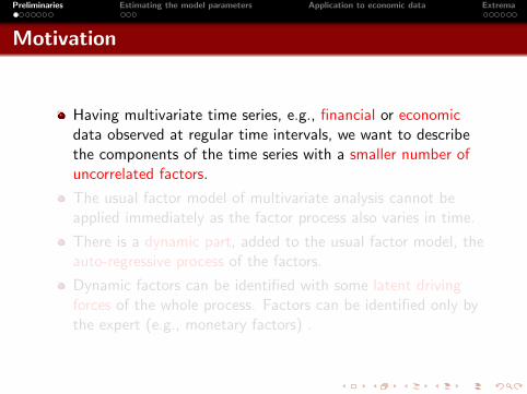
Motivation
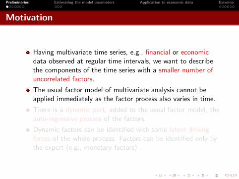
Having multivariate time series, e.g., financial or economicdata observed at regular time intervals, we want to describethe components of the time series with a smaller number ofuncorrelated factors.
The usual factor model of multivariate analysis cannot beapplied immediately as the factor process also varies in time.
There is a dynamic part, added to the usual factor model, theauto-regressive process of the factors.
Dynamic factors can be identified with some latent drivingforces of the whole process. Factors can be identified only bythe expert (e.g., monetary factors) .
Preliminaries Estimating the model parameters Application to economic data Extrema
Motivation
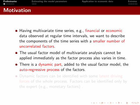
Having multivariate time series, e.g., financial or economicdata observed at regular time intervals, we want to describethe components of the time series with a smaller number ofuncorrelated factors.
The usual factor model of multivariate analysis cannot beapplied immediately as the factor process also varies in time.
There is a dynamic part, added to the usual factor model, theauto-regressive process of the factors.
Dynamic factors can be identified with some latent drivingforces of the whole process. Factors can be identified only bythe expert (e.g., monetary factors) .
Preliminaries Estimating the model parameters Application to economic data Extrema
Motivation
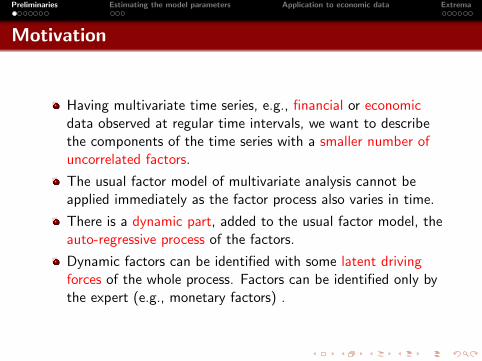
Having multivariate time series, e.g., financial or economicdata observed at regular time intervals, we want to describethe components of the time series with a smaller number ofuncorrelated factors.
The usual factor model of multivariate analysis cannot beapplied immediately as the factor process also varies in time.
There is a dynamic part, added to the usual factor model, theauto-regressive process of the factors.
Dynamic factors can be identified with some latent drivingforces of the whole process. Factors can be identified only bythe expert (e.g., monetary factors) .
Preliminaries Estimating the model parameters Application to economic data Extrema
Motivation
Having multivariate time series, e.g., financial or economicdata observed at regular time intervals, we want to describethe components of the time series with a smaller number ofuncorrelated factors.
The usual factor model of multivariate analysis cannot beapplied immediately as the factor process also varies in time.
There is a dynamic part, added to the usual factor model, theauto-regressive process of the factors.
Dynamic factors can be identified with some latent drivingforces of the whole process. Factors can be identified only bythe expert (e.g., monetary factors) .
Preliminaries Estimating the model parameters Application to economic data Extrema
Remarks
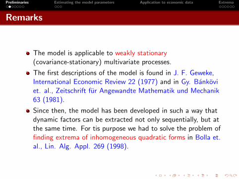
The model is applicable to weakly stationary(covariance-stationary) multivariate processes.
The first descriptions of the model is found in J. F. Geweke,International Economic Review 22 (1977) and in Gy. Bankoviet. al., Zeitschrift fur Angewandte Mathematik und Mechanik63 (1981).
Since then, the model has been developed in such a way thatdynamic factors can be extracted not only sequentially, but atthe same time. For tis purpose we had to solve the problem offinding extrema of inhomogeneous quadratic forms in Bolla et.al., Lin. Alg. Appl. 269 (1998).
Preliminaries Estimating the model parameters Application to economic data Extrema
The model
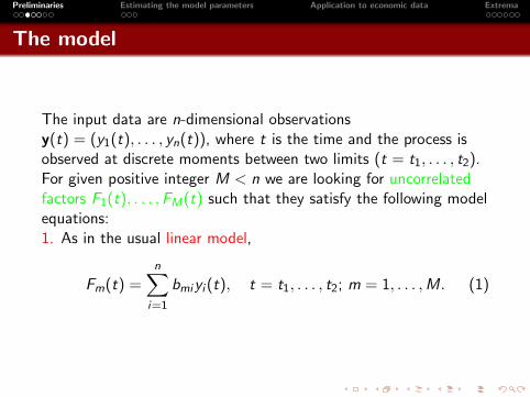
The input data are n-dimensional observationsy(t) = (y1(t), . . . , yn(t)), where t is the time and the process isobserved at discrete moments between two limits (t = t1, . . . , t2).For given positive integer M < n we are looking for uncorrelatedfactors F1(t), . . . ,FM(t) such that they satisfy the following modelequations:1. As in the usual linear model,
Fm(t) =n∑
i=1
bmiyi (t), t = t1, . . . , t2; m = 1, . . . ,M. (1)
Preliminaries Estimating the model parameters Application to economic data Extrema
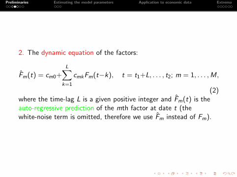
2. The dynamic equation of the factors:
Fm(t) = cm0+L∑
k=1
cmkFm(t−k), t = t1+L, . . . , t2; m = 1, . . . ,M,
(2)where the time-lag L is a given positive integer and Fm(t) is theauto-regressive prediction of the mth factor at date t (thewhite-noise term is omitted, therefore we use Fm instead of Fm).
Preliminaries Estimating the model parameters Application to economic data Extrema
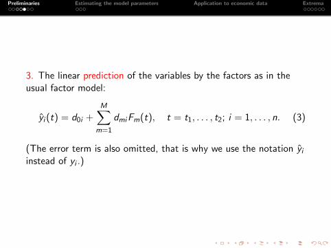
3. The linear prediction of the variables by the factors as in theusual factor model:
yi (t) = d0i +M∑
m=1
dmiFm(t), t = t1, . . . , t2; i = 1, . . . , n. (3)
(The error term is also omitted, that is why we use the notation yi
instead of yi .)
Preliminaries Estimating the model parameters Application to economic data Extrema
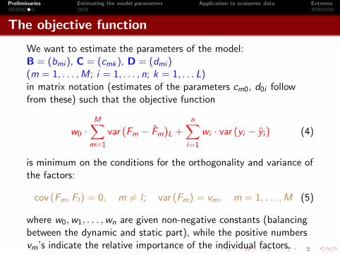
The objective function
We want to estimate the parameters of the model:B = (bmi ), C = (cmk), D = (dmi )(m = 1, . . . ,M; i = 1, . . . , n; k = 1, . . . L)in matrix notation (estimates of the parameters cm0, d0i followfrom these) such that the objective function
w0 ·M∑
m=1
var (Fm − Fm)L +n∑
i=1
wi · var (yi − yi ) (4)
is minimum on the conditions for the orthogonality and variance ofthe factors:
cov (Fm,Fl) = 0, m 6= l ; var (Fm) = vm, m = 1, . . . ,M (5)
where w0,w1, . . . ,wn are given non-negative constants (balancingbetween the dynamic and static part), while the positive numbersvm’s indicate the relative importance of the individual factors.
Preliminaries Estimating the model parameters Application to economic data Extrema
Notation
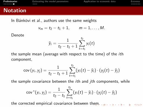
In Bankovi et al., authors use the same weights
vm = t2 − t1 + 1, m = 1, . . . ,M.
Denote
yi =1
t2 − t1 + 1
t2∑t=t1
yi (t)
the sample mean (average with respect to the time) of the ithcomponent,
cov (yi , yj) =1
t2 − t1 + 1
t2∑t=t1
(yi (t)− yi ) · (yj(t)− yj)
the sample covariance between the ith and jth components, while
cov ∗(yi , yj) =1
t2 − t1
t2∑t=t1
(yi (t)− yi ) · (yj(t)− yj)
the corrected empirical covariance between them.
Preliminaries Estimating the model parameters Application to economic data Extrema
Estimating the model parameters
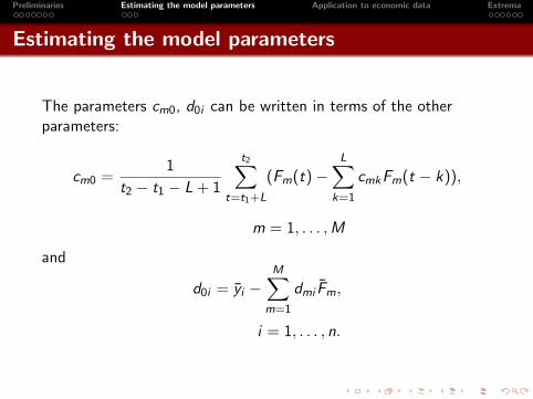
The parameters cm0, d0i can be written in terms of the otherparameters:
cm0 =1
t2 − t1 − L + 1
t2∑t=t1+L
(Fm(t)−L∑
k=1
cmkFm(t − k)),
m = 1, . . . ,M
and
d0i = yi −M∑
m=1
dmi Fm,
i = 1, . . . , n.
Preliminaries Estimating the model parameters Application to economic data Extrema
Further notation
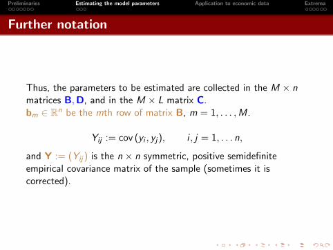
Thus, the parameters to be estimated are collected in the M × nmatrices B,D, and in the M × L matrix C.bm ∈ Rn be the mth row of matrix B, m = 1, . . . ,M.
Yij := cov (yi , yj), i , j = 1, . . . n,
and Y := (Yij) is the n × n symmetric, positive semidefiniteempirical covariance matrix of the sample (sometimes it iscorrected).
Preliminaries Estimating the model parameters Application to economic data Extrema
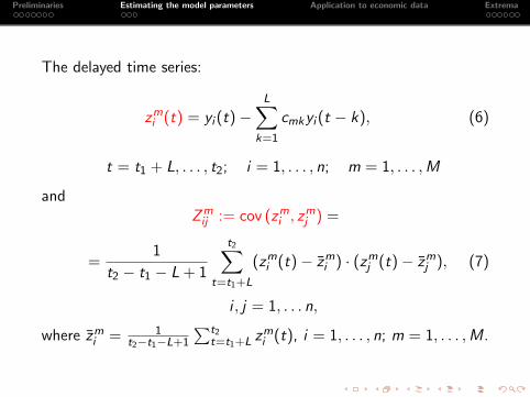
The delayed time series:
zmi (t) = yi (t)−
L∑k=1
cmkyi (t − k), (6)
t = t1 + L, . . . , t2; i = 1, . . . , n; m = 1, . . . ,M
andZm
ij := cov (zmi , zm
j ) =
=1
t2 − t1 − L + 1
t2∑t=t1+L
(zmi (t)− zm
i ) · (zmj (t)− zm
j ), (7)
i , j = 1, . . . n,
where zmi = 1
t2−t1−L+1
∑t2t=t1+L zm
i (t), i = 1, . . . , n; m = 1, . . . ,M.
Preliminaries Estimating the model parameters Application to economic data Extrema
The objective function revisited
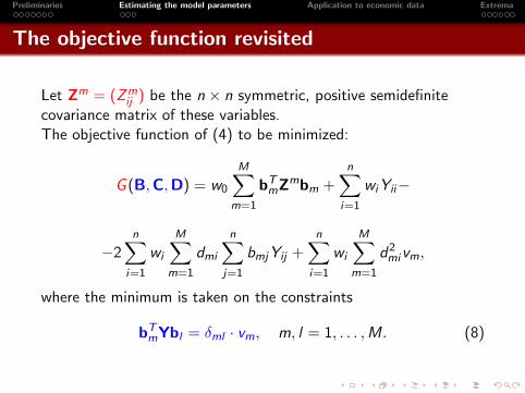
Let Zm = (Zmij ) be the n × n symmetric, positive semidefinite
covariance matrix of these variables.The objective function of (4) to be minimized:
G (B,C,D) = w0
M∑m=1
bTmZmbm +
n∑i=1
wiYii−
−2n∑
i=1
wi
M∑m=1
dmi
n∑j=1
bmjYij +n∑
i=1
wi
M∑m=1
d2mivm,
where the minimum is taken on the constraints
bTmYbl = δml · vm, m, l = 1, . . . ,M. (8)
Preliminaries Estimating the model parameters Application to economic data Extrema
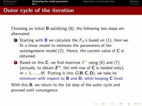
Outer cycle of the iteration
Choosing an initial B satisfying (8), the following two steps arealternated:
1 Starting with B we calculate the Fm’s based on (1), then wefit a linear model to estimate the parameters of theautoregressive model (2). Hence, the current value of C isobtained.
2 Based on this C, we find matrices Zm using (6) and (7)(actually, to obtain Zm, the mth row of C is needed only),m = 1, . . . ,M. Putting it into G (B,C,D), we take itsminimum with respect to B and D, while keeping C fixed.
With this B, we return to the 1st step of the outer cycle andproceed until convergence.
Preliminaries Estimating the model parameters Application to economic data Extrema
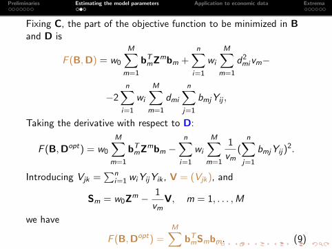
Fixing C, the part of the objective function to be minimized in Band D is
F (B,D) = w0
M∑m=1
bTmZmbm +
n∑i=1
wi
M∑m=1
d2mivm−
−2n∑
i=1
wi
M∑m=1
dmi
n∑j=1
bmjYij ,
Taking the derivative with respect to D:
F (B,Dopt) = w0
M∑m=1
bTmZmbm −
n∑i=1
wi
M∑m=1
1
vm(
n∑j=1
bmjYij)2.
Introducing Vjk =∑n
i=1 wiYijYik , V = (Vjk), and
Sm = w0Zm − 1
vmV, m = 1, . . . ,M
we have
F (B,Dopt) =M∑
m=1
bTmSmbm. (9)
Preliminaries Estimating the model parameters Application to economic data Extrema
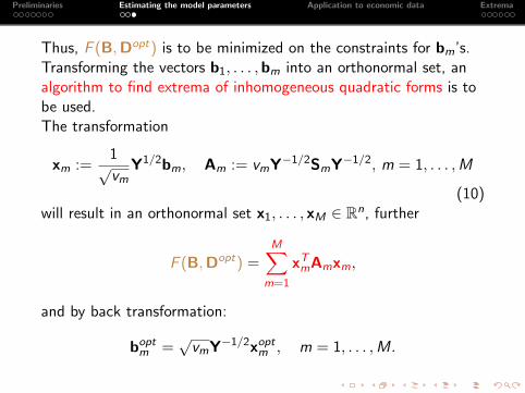
Thus, F (B,Dopt) is to be minimized on the constraints for bm’s.Transforming the vectors b1, . . . ,bm into an orthonormal set, analgorithm to find extrema of inhomogeneous quadratic forms is tobe used.The transformation
xm :=1
√vm
Y1/2bm, Am := vmY−1/2SmY−1/2, m = 1, . . . ,M
(10)will result in an orthonormal set x1, . . . , xM ∈ Rn, further
F (B,Dopt) =M∑
m=1
xTmAmxm,
and by back transformation:
boptm =
√vmY−1/2xopt
m , m = 1, . . . ,M.
Preliminaries Estimating the model parameters Application to economic data Extrema
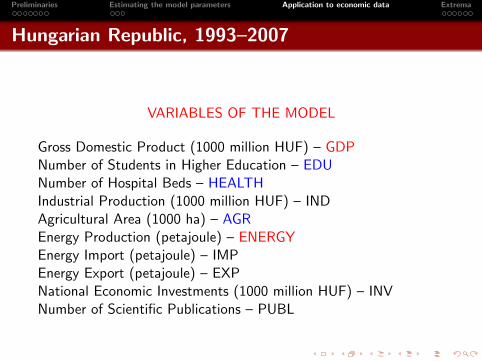
Hungarian Republic, 1993–2007
VARIABLES OF THE MODEL
Gross Domestic Product (1000 million HUF) – GDPNumber of Students in Higher Education – EDUNumber of Hospital Beds – HEALTHIndustrial Production (1000 million HUF) – INDAgricultural Area (1000 ha) – AGREnergy Production (petajoule) – ENERGYEnergy Import (petajoule) – IMPEnergy Export (petajoule) – EXPNational Economic Investments (1000 million HUF) – INVNumber of Scientific Publications – PUBL
Preliminaries Estimating the model parameters Application to economic data Extrema
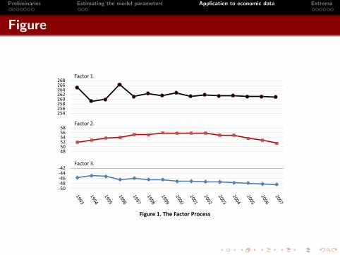
Figure
254256258260262264266268
Figure 1. The Factor Process
-50-48-46-44-42
Factor 3.
Factor 1.
485052545658
Factor 2.
Preliminaries Estimating the model parameters Application to economic data Extrema
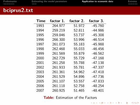
bciprus2.txt
Time factor 1. factor 2. factor 3.1993 264.977 51.972 -45.7601994 259.219 52.811 -44.9861995 259.846 53.737 -45.3081996 266.300 53.996 -46.5141997 261.073 55.183 -45.9881998 262.468 55.033 -46.4561999 261.569 55.879 -46.5622000 262.729 55.729 -47.1682001 261.258 55.788 -47.1382002 261.933 55.781 -47.3372003 261.361 54.962 -47.4182004 261.529 54.896 -47.7362005 261.107 53.557 -47.8332006 261.118 52.758 -48.2542007 260.925 51.465 -48.401
Table: Estimation of the Factors
Preliminaries Estimating the model parameters Application to economic data Extrema
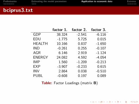
bciprus3.txt
factor 1. factor 2. factor 3.GDP 38.324 -2.541 -6.116EDU -1.775 5.725 0.015HEALTH 10.166 0.837 -1.650IND -0.261 0.255 -0.107AGR 6.146 2.919 -1.124ENERGY 24.082 4.592 -4.054IMP 1.560 -1.209 -0.213EXP -3.907 -0.233 0.615INV 2.864 0.038 -0.510PUBL -0.608 0.197 0.089
Table: Factor Loadings (matrix B)
Preliminaries Estimating the model parameters Application to economic data Extrema
bciprus4.txt
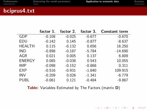
factor 1. factor 2. factor 3. Constant termGDP -0.108 -0.025 -0.677 -0.670EDU -0.142 0.145 -0.877 -8.637HEALTH 0.115 -0.132 0.656 16.250IND -0.898 -0.187 -5.784 -14.690AGR 0.021 0.005 0.137 6.809ENERGY 0.085 -0.038 0.543 10.055IMP -0.098 -0.152 -0.868 0.311EXP -0.516 -0.931 -1.840 109.915INV -0.209 0.026 -1.341 -6.779PUBL -0.061 0.121 -0.484 -9.867
Table: Variables Estimated by The Factors (matrix D)
Preliminaries Estimating the model parameters Application to economic data Extrema
bciprus5.txt
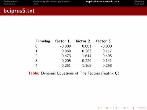
Timelag factor 1. factor 2. factor 3.0 -0.000 0.001 -0.0001 0.069 0.283 0.1172 0.473 1.644 0.4953 0.205 0.229 0.1414 0.251 -1.168 0.258
Table: Dynamic Equations of The Factors (matrix C)
Preliminaries Estimating the model parameters Application to economic data Extrema
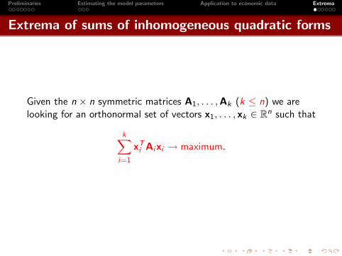
Extrema of sums of inhomogeneous quadratic forms
Given the n × n symmetric matrices A1, . . . ,Ak (k ≤ n) we arelooking for an orthonormal set of vectors x1, . . . , xk ∈ Rn such that
k∑i=1
xTi Aixi → maximum.
Preliminaries Estimating the model parameters Application to economic data Extrema
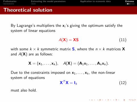
Theoretical solution
By Lagrange’s multipliers the xi ’s giving the optimum satisfy thesystem of linear equations
A(X) = XS (11)
with some k × k symmetric matrix S, where the n × k matrices Xand A(X) are as follows:
X = (x1, . . . , xk), A(X) = (A1x1, . . . ,Akxk).
Due to the constraints imposed on x1, . . . , xk , the non-linearsystem of equations
XTX = Ik (12)
must also hold.
Preliminaries Estimating the model parameters Application to economic data Extrema
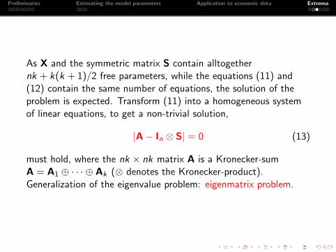
As X and the symmetric matrix S contain alltogethernk + k(k + 1)/2 free parameters, while the equations (11) and(12) contain the same number of equations, the solution of theproblem is expected. Transform (11) into a homogeneous systemof linear equations, to get a non-trivial solution,
|A− In ⊗ S| = 0 (13)
must hold, where the nk × nk matrix A is a Kronecker-sumA = A1 ⊕ · · · ⊕ Ak (⊗ denotes the Kronecker-product).Generalization of the eigenvalue problem: eigenmatrix problem.
Preliminaries Estimating the model parameters Application to economic data Extrema
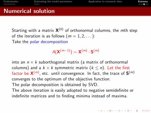
Numerical solution
Starting with a matrix X(0) of orthonormal columns, the mth stepof the iteration is as follows (m = 1, 2, . . . ):Take the polar decomposition
A(X(m−1)) = X(m) · S(m)
into an n × k suborthogonal matrix (a matrix of orthonormalcolumns) and a k × k symmetric matrix (k ≤ n). Let the firstfactor be X(m), etc. until convergence. In fact, the trace of S(m)
converges to the optimum of the objective function.The polar decomposition is obtained by SVD.The above iteration is easily adopted to negative semidefinite orindefinite matrices and to finding minima instead of maxima.
Preliminaries Estimating the model parameters Application to economic data Extrema
References
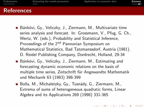
Bankovi, Gy., Veliczky, J., Ziermann, M., Multivariate timeseries analysis and forecast. In: Grossmann, V., Pfug, G. Ch.,Wertz, W. (eds.), Probability and Statistical Inference,Proceedings of the 2nd Pannonian Symposium onMathematical Statistics, Bad Tatzmanssdorf, Austria (1981).D. Reidel Publishing Company, Dordrecht, Holland, 29-34
Bankovi, Gy., Veliczky, J., Ziermann, M., Estimating andforecasting dynamic economic relations on the basis ofmultiple time series, Zeitschrift fur Angewandte Mathematikund Mechanik 63 (1983) 398-399
Bolla, M., Michaletzky, Gy., Tusnady, G., Ziermann, M.,Extrema of sums of heterogeneous quadratic forms, LinearAlgebra and its Applications 269 (1998) 331-365
Preliminaries Estimating the model parameters Application to economic data Extrema
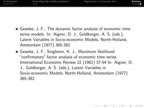
Geweke, J. F., The dynamic factor analysis of economic timeseries models. In: Aigner, D. J., Goldberger, A. S. (eds.),Latent Variables in Socio-economic Models, North-Holland,Amsterdam (1977) 365-382
Geweke, J. F., Singleton, K. J., Maximum likelihood“confirmatory” factor analysis of economic time series,International Economic Review 22 (1981) 37-54 In: Aigner, D.J., Goldberger, A. S. (eds.), Latent Variables inSocio-economic Models, North-Holland, Amsterdam (1977)365-382