Electronic copy available at: http://ssrn.com/abstract=1140900

Dynamic Marketing Mix Allocation for Long-Term

Profitability

Ricardo Montoya∗

Oded Netzer

Kamel Jedidi

December 16, 2007

∗Ricardo Montoya is a doctoral candidate at the Graduate School of Business, Columbia University (email:rm2183@columbia.edu). Oded Netzer is an Assistant Professor of Marketing at the Graduate School of Business,Columbia University (email: on2110@columbia.edu). Kamel Jedidi is a Professor of Marketing at the Graduate Schoolof Business, Columbia University (email: kj7@columbia.edu). Please address all correspondence to Ricardo Montoya,Graduate School of Business, Columbia University, 3022 Broadway, 311 Uris Hall, New York, NY 10027, USA.

Electronic copy available at: http://ssrn.com/abstract=1140900

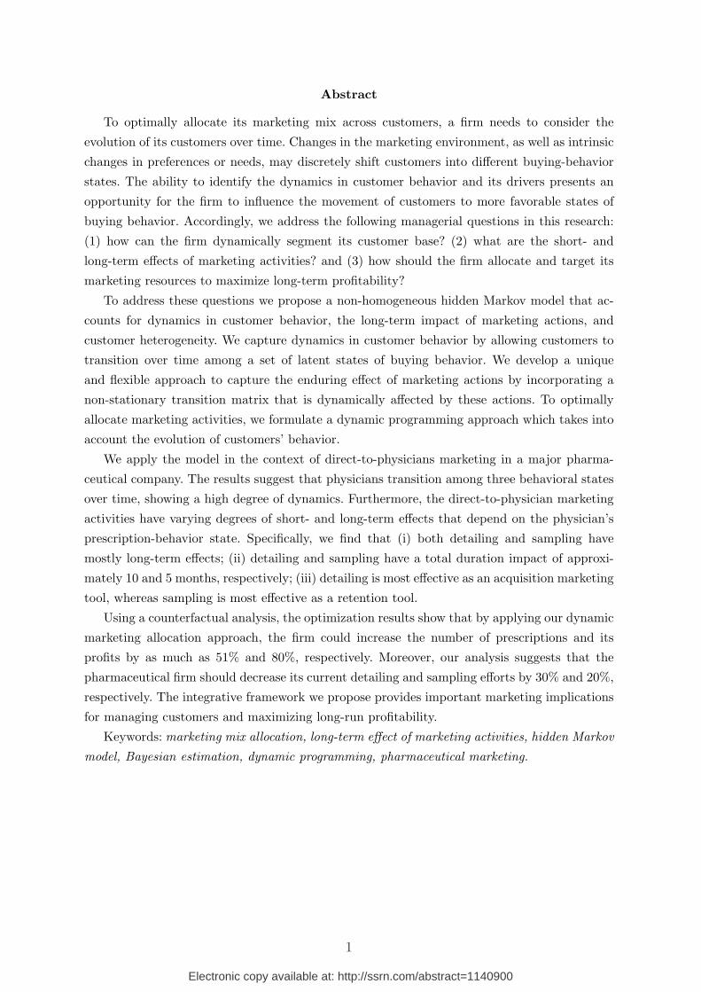
Abstract

To optimally allocate its marketing mix across customers, a firm needs to consider the

evolution of its customers over time. Changes in the marketing environment, as well as intrinsic

changes in preferences or needs, may discretely shift customers into different buying-behavior

states. The ability to identify the dynamics in customer behavior and its drivers presents an

opportunity for the firm to influence the movement of customers to more favorable states of

buying behavior. Accordingly, we address the following managerial questions in this research:

(1) how can the firm dynamically segment its customer base? (2) what are the short- and

long-term effects of marketing activities? and (3) how should the firm allocate and target its

marketing resources to maximize long-term profitability?

To address these questions we propose a non-homogeneous hidden Markov model that ac-

counts for dynamics in customer behavior, the long-term impact of marketing actions, and

customer heterogeneity. We capture dynamics in customer behavior by allowing customers to

transition over time among a set of latent states of buying behavior. We develop a unique

and flexible approach to capture the enduring effect of marketing actions by incorporating a

non-stationary transition matrix that is dynamically affected by these actions. To optimally

allocate marketing activities, we formulate a dynamic programming approach which takes into

account the evolution of customers’ behavior.

We apply the model in the context of direct-to-physicians marketing in a major pharma-

ceutical company. The results suggest that physicians transition among three behavioral states

over time, showing a high degree of dynamics. Furthermore, the direct-to-physician marketing

activities have varying degrees of short- and long-term effects that depend on the physician’s

prescription-behavior state. Specifically, we find that (i) both detailing and sampling have

mostly long-term effects; (ii) detailing and sampling have a total duration impact of approxi-

mately 10 and 5 months, respectively; (iii) detailing is most effective as an acquisition marketing

tool, whereas sampling is most effective as a retention tool.

Using a counterfactual analysis, the optimization results show that by applying our dynamic

marketing allocation approach, the firm could increase the number of prescriptions and its

profits by as much as 51% and 80%, respectively. Moreover, our analysis suggests that the

pharmaceutical firm should decrease its current detailing and sampling efforts by 30% and 20%,

respectively. The integrative framework we propose provides important marketing implications

for managing customers and maximizing long-run profitability.

Keywords: marketing mix allocation, long-term effect of marketing activities, hidden Markov

model, Bayesian estimation, dynamic programming, pharmaceutical marketing.

1

1. Introduction

“The pharmaceutical industry is under significant pressure to consider its costs

very carefully. Since marketing budgets often represent a major proportion of a com-

pany’s cost base, they can easily become the target of budget cuts. Although marketing

investments are profitable, in the main, returns are now under intense scrutiny with

all budgets being squeezed. The pressure to measure marketing return and effective-

ness has never been stronger. Currently, much budget is spent despite marketers

being unable to identify which combination of activities has the greatest growth po-

tential, and without knowing what specific effect individual activities are having on

physicians over time.” — Andree Bates (2006)

In order to stay competitive, firms need to wisely allocate marketing mix resources with the

objective of establishing and sustaining long-term relationships with their customers. In doing

so, managers should consider how a given marketing budget should be allocated across different

marketing activities, customers, and time. However, marketing resource allocation decisions are

complicated and managers tend to address them with fairly arbitrary simplified heuristics and

decision rules (Mantrala 2002). Such rules usually result in sub-optimal decisions, which could

lead to a significant waste of resources. Improving these decisions could have a direct impact

on long-term profitability.

When making marketing allocation decisions, firms often face the problem of trading off

between short- and long-term revenues. For example, Harrah’s, through its Total Rewards

loyalty program, may offer a free dinner to customers who are having a “bad day”. Such a

marketing action pulls gamblers away from the casino, producing a short-term loss of revenues.

In doing so, however, the casino expects to bring future revenues by shifting the customers to

a more favorable state of relationship with Harrah’s. Similarly, Procter & Gamble faces such

trade-offs when giving free samples of Pampers diapers. Though this action cannibalizes current

purchases, the company hopes to have a long-term impact by increasing its customer base with

customers who otherwise would have not tried the product. American Airlines may offer to

current customers either last-minute deals or free upgrades in order to fill empty first-class

seats. A last-minute deal creates immediate revenues for the company, whereas a free upgrade

produces an opportunity cost and additional service costs to current operations. In choosing the

free upgrade, however, the company anticipates an increase in customer loyalty and long-term

2

profits.

In these examples, a successful marketing mix allocation at the individual level could en-

hance customer equity and, therefore, constitutes an important tool for managing the firm’s

customer base. However, these examples demonstrate that the task of allocating resources at

the individual level is complicated and requires the knowledge of individual customer behavior

and responsiveness to marketing interventions over time. The resource allocation task becomes

even more complicated when firms have multiple marketing interventions with varying degrees

of short- and long-term effects, and when customers have evolving preferences and sensitivities.

Understanding customer dynamics and the varying impact of marketing activities is critical

for optimizing marketing decisions. Ignoring such dynamics can result in misleading inferences

regarding the temporal pattern of elasticities. A firm that is myopic and does not consider the

long-term effect of its marketing interventions is likely to under allocate marketing interven-

tions with relatively small short-term effects but substantial long-term effects, such as the ones

described above. Similarly, a firm that is forward-looking in its marketing mix allocation, but

does not capture well the evolution of customer preferences and buying behavior over time, is

likely to allocate its marketing mix sub-optimally.

This paper proposes an integrative resource allocation approach that simultaneously con-

siders a forward-looking, individual-level allocation of marketing resources, where customers’

preferences change over time, and the firm can influence the dynamics in customers’ preferences

using multiple marketing interventions with both short- and long-term effects. Our approach

is built around a non-homogeneous hidden Markov model (HMM) that accounts for dynamics

in customer behavior and the long-term impact of marketing actions. We capture dynamics in

customer behavior by allowing customers to transition over time among a set of latent states

of buying behavior. We model the enduring impact of marketing actions by incorporating a

non-homogeneous transition matrix that is dynamically affected by these actions. To optimally

allocate and target marketing resources and to maximize long-term profitability, we propose a

stochastic dynamic programming approach which takes into account customer heterogeneity,

the evolution in customers’ behavior, the short- and long-term effects of marketing interven-

tions, and the long-term payoff.

This paper is organized as follows: Section 2 motivates the need to consider the dynamics

in customer behavior and the short- and long-term effects of marketing actions in marketing

3

mix resource allocation. Section 3 presents the modeling approach proposed for capturing the

dynamics in customer-buying behavior, the response to marketing mix interventions, and the

dynamic optimal marketing mix allocation. Section 4 illustrates the proposed model using

direct-to-physicians marketing data from a major pharmaceutical company. Section 5 concludes

by discussing practical implications, theoretical contributions, and future directions.

2. Marketing Mix Allocation and Dynamic Customer

Management

In recent years there has been an increasing interest in the study of marketing mix allocation

problems (Rust and Verhoef 2005). The customer relationship management (CRM) literature

suggests that marketing initiatives should be evaluated by measuring their impact on the long-

term value generated by improving the relationship with the customer. To do so, the firm must

be able to measure the dynamics in customer buying behavior and the long-term impact of

its marketing actions. Indeed, Rust and Chung (2006) highlight the need for an integrative

framework that maximizes long-term profits, accounting for individually targeted marketing

interventions and the joint effect of multiple marketing interventions. Our paper presents such

a framework and contributes to the understanding of how and why customer profitability could

change over time due to intrinsic buying-behavior dynamics and marketing interventions.

Accordingly, in this section we briefly review previous work related to the different com-

ponents of our model: dynamics in customer buying behavior, long-term effect of marketing

activities, and marketing mix allocation.

2.1. Dynamics in Customer Buying Behavior

Several approaches have been suggested to model customer evolution over time. Most of these

use observed variables to capture the dynamics in buying behavior. In the CRM literature, het-

erogeneity and dynamics in customer behavior are often captured using the recency, frequency,

and monetary value (RFM) framework (e.g., Bitran and Mondschein 1996; Colombo and Jiang

1999; Pfeifer and Carraway 2000). RFM analysis is a deterministic approach in which customers

are characterized by how recently they transacted, how frequently they have transacted in the

past, and the value of those transactions. This approach is commonly used in the industry due

4

to its ability to capture dynamics in customer behavior in a relatively simple way. For example,

Pfeifer and Carraway (2000) model customer relationship evolution as a Markov chain, in which

customers transition among several observed states characterized by the RFM variables. While

the RFM approach is useful for a dynamic descriptive segmentation of the firm’s customer base,

it is not obvious how it can be used to capture the dynamic and enduring effects of marketing

actions and to optimize marketing allocation, which are key objectives in our study.

Another common approach to modeling customer evolution using observed states is the

state-dependence model (e.g., Bucklin and Lattin 1991; Guadagni and Little 1983; Heckman

1981; Srinivasan and Kesavan 1976). Our proposed HMM extends the state-dependence model

by allowing the states to be defined not only by past behavior, but also by external factors

such as marketing activities. Ignoring such external effects can lead to overestimation of state-

dependence (Erdem and Sun 2001; Keane 1997). Most models of state-dependence ignore the

long-term effect of marketing variables and are therefore susceptible to this bias. Conversely, a

model that estimates the long-term effect of marketing activities but ignores state-dependence

may overestimate the total effect of marketing interventions. To overcome these limitations and

to simultaneously capture the internal and external sources of dynamics in buying behavior, we

propose a hidden Markov model (HMM; see McDonald and Zucchini 1997 and Rabiner 1989

for a detailed review of HMMs).

There is a small, but increasing, number of applications of HMMs in marketing. For ex-

ample, Liechty et al. (2003) develop a HMM to identify the respondents’ attentional states

when they are exposed to an advertisement viewing task. Montgomery et al. (2004) build a

continuous-time, two-state HMM to investigate how customers move among different categories

of web pages when searching for information online. Du and Kamakura (2006) present a HMM

to capture the dynamic evolution of American families’ lifecycles. Moon et al. (2007) use a

HMM to model unobserved competitors’ marketing actions in a pharmaceutical context. Net-

zer et al. (2007) analyze the dynamic relationship between alumni and their university, allowing

for different states of relationship with the university which affect donation behavior. With the

exception of Netzer et al. (2007), the applications above assume a homogeneous HMM char-

acterized by a stationary transition matrix. In our framework, allowing for a non-stationary

transition matrix is crucial since it allows one to capture the enduring effects of marketing ac-

tivities, and disentangle them from the short-term effects. Unlike Netzer et al. (2007) – who do

5

not incorporate firm’s initiated marketing actions – our model captures the effect of marketing

interventions on customer dynamics and derives an optimal marketing allocation strategy for

these interventions.

2.2. Short- and Long-Term Effects of Marketing Activities

Customers may exhibit dynamics not only due to the intrinsic evolution in their buying-

behavior, but also due to the long-term impact of the firm’s actions. Furthermore, to optimally

allocate marketing activities, firms need to consider both customer dynamics and the short-

and long-term effects of their actions.

One can divide the literature analyzing the long-term effect of marketing actions into mass

marketing and direct marketing. Several studies have analyzed the long-term effect of mass

marketing activities such as advertising and price promotions (Dekimpe and Hanssens 1995,

1999; Dekimpe et al. 2005; Jedidi et al. 1999; Mela et al. 1997). Most of these studies assume a

stable market (Mela et al. 1997; Papatla and Krishnamurthi 1996) and use a Koyck-type model,

which implies that performance will return to its pre-marketing intervention level. Dekimpe and

Hanssens (1995) and Dekimpe et al. (2005), on the other hand, have examined the effect of

marketing actions in evolving markets using a persistence modeling approach to capture long-

term changes in performance. Since the studies above investigate the short- and long-term effect

of mass marketing actions, the issue of optimal allocation and targeting of these activities is

rarely addressed.

In contrast, most of the direct marketing literature is interested in the targeting and allo-

cation of marketing activities (Bitran and Mondschein 1996; Elsner et al. 2004; Gonul and Ter

Hofstede 2006; Roberts and Berger 1999). However, this literature often ignores the possibly

long-term effects of the marketing interventions when solving the marketing allocation problem.

Some exceptions can be found in the context of catalog mailing decisions. For instance, Gonul

and Shi (1998) present a structural dynamic programming approach where customers optimize

a dynamic Markov game, by contemplating how their purchase decisions will affect the firm’s

future marketing decisions. Simester et al. (2006) present a nonparametric approach to capture

customers’ dynamics and the long-term effect of marketing actions. They provide a dynamic

programming problem that the firm solves in order to mail catalogs to its customers. Our pa-

per extends these papers by presenting a non-homogeneous HMM framework to capture the

long-term effects of multiple marketing actions and their influence on customer dynamics. Our

6

approach pushes forward the literature by allowing us to disentangle short-term and long-term

effects, and take advantage of their influence at the individual level when allocating marketing

resources.

2.3. Marketing Mix Allocation

The marketing mix allocation literature could generally be divided based on the portfolio of

marketing mix interventions allocated and the level of aggregation in allocating the marketing

mix. The direct marketing literature often deals with a single marketing activity such as cata-

log mailing (Bitran and Mondschein 1996; Gonul and Shi 1998; Gonul and Ter Hofstede 2006;

Simester et al. 2006), optimal pricing decisions (Lewis 2005), and couponing decisions (Bawa

and Shoemaker 1987; Rossi et al. 1996). These studies often deal with optimization without

budget constraints when making such allocation decisions. Mass marketing mix allocation stud-

ies, on the other hand, typically consider a pair of marketing actions, with or without their

synergies. For example, advertising and promotion (Jedidi et al. 1999; Mela et al. 1997, Naik

et al. 2005), sales force and advertising (Gatignon and Hanssens 1987), or advertising between

different media channels (Naik et al. 1998). In contrast to the direct marketing literature, these

studies involve aggregate allocation of mass marketing mix interventions. Most of these studies

do not account for changes in marketing mix sensitivity over time. In this paper, we extend the

literature on marketing mix allocation by offering an integrative approach for managing cus-

tomers through an optimal allocation of multiple, individually-targeted, marketing actions for

long-run profitability. We do so, while taking into account heterogeneous changes in customer

behavior and dynamic response to marketing interventions, and considering the possibility of

budget constraints.

3. Model Development

To model the dynamics in buying behavior and the short- and long-term effects of marketing

activities we build a HMM. In our model, customers can transition among a set of buying-

behavior states, where the transition between the states, as well as the buying behavior given

a state, are affected by multiple marketing activities. We consider two aspects of customer

heterogeneity: customers could differ in terms of their propensity of being in each of the states

and in their response to marketing interventions. To optimally allocate marketing resources

7

across customers, we solve a stochastic dynamic programming (DP) problem, accounting for

customers’ heterogeneity and dynamics, and maximizing customer value for a given planning

horizon. We use a partially observed markov decision process (POMDP) to capture stochasticity

in the customer’s buying-behavior state membership. In this section, we first describe how our

modeling approach captures customer dynamics through a HMM. We then explain how the

HMM can capture both short- and long-term effects of marketing actions. We conclude this

section with a description of how one can use our proposed model and the POMDP to optimize

marketing mix allocation.

3.1. Customer Dynamics: The Hidden Markov Model

We assume a set of customers who make repeated purchases and are exposed to marketing

activities initiated by the firm, both of which are observed by the researcher over time. We define

a finite set of buying-behavior states that can be characterized by the intrinsic preference for

the product, the purchase propensity, and the responsiveness to different marketing initiatives.

For instance, let us assume two buying-behavior states. At the low buying-behavior state,

customers make only few purchases, possibly due to the need to acquire information about

the product. Consequently, customers in this state may be responsive to marketing initiatives

that provide information (e.g., advertising and free samples). In contrast, customers at the

higher buying-behavior state, which corresponds to high purchase frequency, are likely to be

affected by marketing initiatives aimed at keeping customers engaged (e.g., loyalty programs

and free upgrades). Furthermore, marketing initiatives not only affect customer behavior at

each buying-behavior state, but may also trigger the transitions between these states. For

example, free samples may induce customers to try the product and move them from the low

buying-behavior state to the higher state. In contrast, increasing price or making it difficult for

customers to redeem rewards in the loyalty program, may induce customers to switch from the

high buying-behavior state to the lower one.

Buying-behavior states are often not observed and therefore need to be inferred from cus-

tomers’ observed behavior. Accordingly, we propose a HMM which is built of a set of latent

buying-behavior states. Customers can stochastically transition among the buying-behavior

states through a Markovian first-order process. The transitions between the states are a func-

tion of marketing mix activities. We relate the unobserved buying-behavior states to the ob-

served choices through a state-dependent component, which captures the short-term effect of

8

different marketing initiatives on buying behavior conditioned on the current customer state.

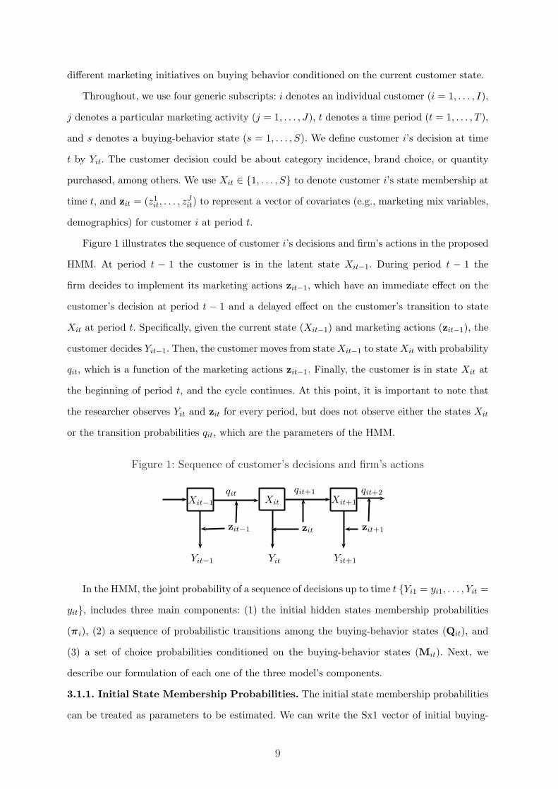
Throughout, we use four generic subscripts: i denotes an individual customer (i = 1, . . . , I),

j denotes a particular marketing activity (j = 1, . . . , J), t denotes a time period (t = 1, . . . , T ),

and s denotes a buying-behavior state (s = 1, . . . , S). We define customer i’s decision at time

t by Yit. The customer decision could be about category incidence, brand choice, or quantity

purchased, among others. We use Xit ∈ {1, . . . , S} to denote customer i’s state membership at

time t, and zit = (z1it, . . . , z

Jit) to represent a vector of covariates (e.g., marketing mix variables,

demographics) for customer i at period t.

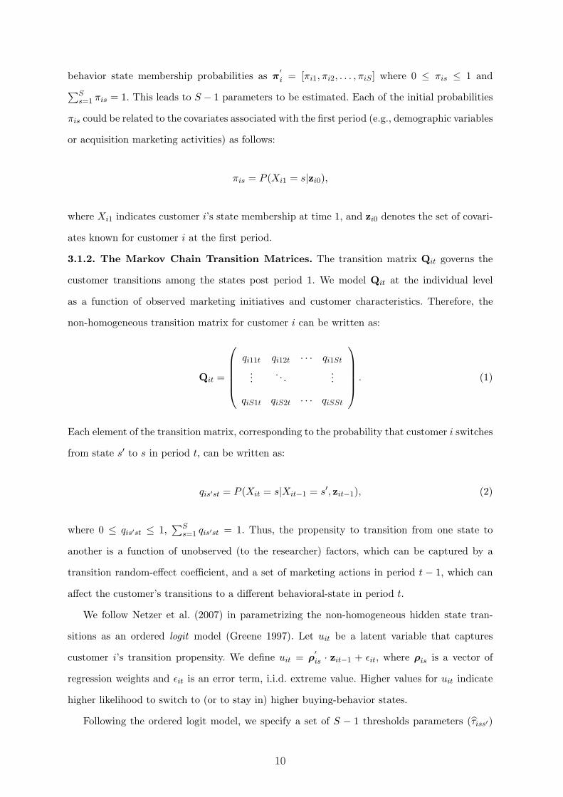
Figure 1 illustrates the sequence of customer i’s decisions and firm’s actions in the proposed

HMM. At period t − 1 the customer is in the latent state Xit−1. During period t − 1 the

firm decides to implement its marketing actions zit−1, which have an immediate effect on the

customer’s decision at period t − 1 and a delayed effect on the customer’s transition to state

Xit at period t. Specifically, given the current state (Xit−1) and marketing actions (zit−1), the

customer decides Yit−1. Then, the customer moves from state Xit−1 to state Xit with probability

qit, which is a function of the marketing actions zit−1. Finally, the customer is in state Xit at

the beginning of period t, and the cycle continues. At this point, it is important to note that

the researcher observes Yit and zit for every period, but does not observe either the states Xit

or the transition probabilities qit, which are the parameters of the HMM.

Figure 1: Sequence of customer’s decisions and firm’s actions

zit−1

Yit−1

zit zit+1

qitqit+1

Yit Yit+1

Xit−1 Xit Xit+1

qit+2

In the HMM, the joint probability of a sequence of decisions up to time t {Yi1 = yi1, . . . , Yit =

yit}, includes three main components: (1) the initial hidden states membership probabilities

(πi), (2) a sequence of probabilistic transitions among the buying-behavior states (Qit), and

(3) a set of choice probabilities conditioned on the buying-behavior states (Mit). Next, we

describe our formulation of each one of the three model’s components.

3.1.1. Initial State Membership Probabilities. The initial state membership probabilities

can be treated as parameters to be estimated. We can write the Sx1 vector of initial buying-

9

behavior state membership probabilities as π′i = [πi1, πi2, . . . , πiS ] where 0 ≤ πis ≤ 1 and

∑Ss=1 πis = 1. This leads to S − 1 parameters to be estimated. Each of the initial probabilities

πis could be related to the covariates associated with the first period (e.g., demographic variables

or acquisition marketing activities) as follows:

πis = P (Xi1 = s|zi0),

where Xi1 indicates customer i’s state membership at time 1, and zi0 denotes the set of covari-

ates known for customer i at the first period.

3.1.2. The Markov Chain Transition Matrices. The transition matrix Qit governs the

customer transitions among the states post period 1. We model Qit at the individual level

as a function of observed marketing initiatives and customer characteristics. Therefore, the

non-homogeneous transition matrix for customer i can be written as:

Qit =

qi11t qi12t · · · qi1St

.... . .

...

qiS1t qiS2t · · · qiSSt

. (1)

Each element of the transition matrix, corresponding to the probability that customer i switches

from state s′ to s in period t, can be written as:

qis′st = P (Xit = s|Xit−1 = s′, zit−1), (2)

where 0 ≤ qis′st ≤ 1,∑S

s=1 qis′st = 1. Thus, the propensity to transition from one state to

another is a function of unobserved (to the researcher) factors, which can be captured by a

transition random-effect coefficient, and a set of marketing actions in period t − 1, which can

affect the customer’s transitions to a different behavioral-state in period t.

We follow Netzer et al. (2007) in parametrizing the non-homogeneous hidden state tran-

sitions as an ordered logit model (Greene 1997). Let uit be a latent variable that captures

customer i’s transition propensity. We define uit = ρ′is · zit−1 + εit, where ρis is a vector of

regression weights and εit is an error term, i.i.d. extreme value. Higher values for uit indicate

higher likelihood to switch to (or to stay in) higher buying-behavior states.

Following the ordered logit model, we specify a set of S − 1 thresholds parameters (τiss′)

10

for each state s, that delineates the regions of switching. For example, consider a three-state

model where customer i is in state 2 in period t−1. If uit ≤ τi21, customer i would transition to

state 1. If τi21 ≤ uit ≤ τi22, customer i would stay in state 2. And if uit ≥ τi22, then customer i

would transition to state 3.

More generally, the transition probabilities in Equation (2) are given by:

qis1t =exp(τis1 − ρ

′is · zit−1)

1 + exp(τis1 − ρ′is · zit−1)

,

qis2t =exp(τis2 − ρ

′is · zit−1)

1 + exp(τis2 − ρ′is · zit−1)

− exp(τis1 − ρ′is · zit−1)

1 + exp(τis1 − ρ′is · zit−1)

, (3)

...

qisSt = 1− exp(τisS−1 − ρ′is · zit−1)

1 + exp(τisS−1 − ρ′is · zit−1)

.

Equation (3) specifies how previous marketing actions and customer characteristics (zit−1)

affect the transition probabilities. To ensure a proper ordering of the buying-behavior states,

we impose a non-decreasing order for the thresholds (τis1 ≤ τis2 ≤ . . . ≤ τisS−1) by setting

τis1 = τis1; τiss′ = τiss′−1 + exp(τiss′) ∀i, s, and s′ = 2, . . . , S − 1.

3.1.3. Conditional Choice Probabilities. If the buying-behavior states are observed, one

could directly estimate the Markov model defined by the transition matrix. Since the states are

not observed, we propose the use of a HMM to uncover the buying-behavior states from the

observed buying behavior. The HMM describes a stochastic process that is not directly observ-

able (the latent state membership), but can be inferred through another stochastic process that

relates the set of observations to the HMM latent state membership. Such observations corre-

spond to the customer’s decisions over time. We model the customer’s decisions conditional on

the customer being in a particular state and the marketing interventions as:1

Pist = P (Yit = yit|Xit = s, zit), (4)

where we allow the marketing actions in period t (zit) to affect the customer’s decision (Yit). Fol-

lowing standard notation in HMM models, we write the vector of state dependent probabilities

1For continuous Yit, Pist corresponds to the pdf f(yit|Xit = s, zit).

11

as a diagonal matrix (Mit):

Mit =

Pi1t 0 · · · 0...

. . ....

0 · · · 0 PiSt

. (5)

3.1.4. The Likelihood of an Observed Sequence of Choices. Given the Markovian struc-

ture of the model, the likelihood of observing a choice at time t is dependent on all choices

made in the past. Therefore, we write the joint likelihood of observing a sequence of T decisions

made by customer i as follows:

LiT = P (Yi1, . . . , Yit, . . . , YiT ) =S∑

Xi1=1

· · ·S∑

XiT =1

P (Yi1, . . . , YiT |Xi1, . . . , XiT )P (Xi1, . . . , XiT ) = (6)

S∑

Xi1=1

· · ·S∑

XiT =1

P (Yi1|Xi1) · · ·P (YiT |XiT )P (Xi1)P (Xi2|Xi1) · · ·P (XiT |XiT−1) =

S∑

Xi1=1

· · ·S∑

XiT =1

P (Xi1)P (Yi1|Xi1)P (Xi2|Xi1)P (Yi2|Xi2) · · ·P (XiT |XiT−1)P (YiT |XiT ).

The population likelihood for a sample of N random customers is given by L =∏N

i=i LiT .

McDonald and Zucchini (1997) show that the above likelihood expression can be succinctly

written as:

L =N∏

i=1

π′iMi1

T∏

t=2

QitMit1, (7)

where 1 is a Sx1 vector of ones.

3.1.5. Recovering State Membership. Our HMM approach allows us to recover the cus-

tomers’ membership to any state at any given time period. We compute the probabilistic

membership using the filtering approach (McDonald and Zucchini 1997), which uses the infor-

mation known up to period t to recover the customer’s membership at period t. The filtering

probability that customer i is in state s at time t, conditioned on the customer’s decisions up

to period t, is given by:

P (Xit = s|Yi1, . . . , Yit) = πiMi1

T∏

t=2

Qitmsit/Lit, (8)

12

where msit is the sth column of the matrix Mit and Lit is the likelihood of the observed sequence

of customer i’s decisions up to time t from Equation (6).

3.2. The Short- and Long-Term Effects of Marketing Activities

Marketing mix interventions can have an immediate impact on the customer’s behavior (e.g.,

product purchase due to sales promotion) with short-term implications and/or produce a change

in the customer’s buying-behavior state, which may have long-term implications (e.g., being

upgraded to a higher tier in the loyalty programs).

Our model allows marketing interventions to have both short- and long-term effects and

disentangles both effects in a very natural way. To capture the short-term effect, marketing ac-

tions are included in the state-dependent decision (zit in Equation (4)). Behaviorally, this means

that conditional on the customer’s current buying-behavior state, marketing interventions may

have an immediate effect on the likelihood and/or the quantity purchased. To capture the

long-term effect, marketing interventions are included in the transition probabilities between

buying-behavior states (zit−1 in Equation (2)).2 Behaviorally, this means that marketing in-

terventions can move a customer from one buying-behavior state to another, possibly more

favorable, state. As illustrated in the previous examples, this regime shift may have long-term

impact on the customer’s decisions depending upon the stickiness of the new state and the

nature of the transitions from it. The set of marketing interventions zit to be included in the

transition matrix (Equation (2)) or in the conditional choice component (Equation (4)) may

be different. The location of the marketing interventions in our model can be determined a pri-

ori based on the researcher’s hypotheses or managerial beliefs, or tested statistically following

model selection criteria. In this paper, we locate the marketing actions in both the transition

matrix Qit and in the conditional choice matrix Mit to empirically assess the degree of short-

and long-term impact of each marketing activity.3

3.3. Optimal Marketing Mix Allocation

In this section, we describe a dynamic programming (DP) optimization procedure used to

optimally allocate and target marketing resources for long-term profitability.

2We include zit−1 in the transition matrix to ensure precedence of zit−1 to the customer’s transition and thecustomer decision in period t. In situations where the customer is exposed to the marketing actions prior to makinga decision in the same period (e.g., scanner panel data), one could replace zit−1 with zit.

3We have conducted a series of simulations to confirm the empirical identification of the short- and long-termeffects. Details can be obtained from the authors.

13

One aspect of the HMM that makes the dynamic optimization difficult is that the firm

has uncertainty regarding the customers’ state at any period t, and how the customers will

evolve over time through the buying-behavior states. In other words, the state variable Xit is

only probabilistically observed. Most of the DP applications in marketing utilize observed state

variables such as past purchases (e.g., Bitran and Mondschein 1996; Simester et al. 2006). To

address this complexity, we define the DP states using a partially observed Markov decision

process (POMDP). A POMDP is a sequential decision problem, pertaining to a dynamic setting,

where the information concerning the state of the system is incomplete (see e.g., Aviv and Pazgal

2005; Lovejoy 1991; Monahan 1982). In our case, the states of the DP problem are defined by

the firm’s beliefs about customers’ state membership. Our approach, however, differs from other

POMDPs described in the literature in that we assume the firm wants to predict the impact of

the marketing interventions for an infinite horizon, not just the next period. This assumption

has implications for how the firm updates its beliefs, as we describe below.

We define bit as the firm’s belief about the probability that customer i is in state s at time

t. After observing the customer’s decision and its own marketing intervention decision (zit),

the firm can update its beliefs in a Bayesian manner. Specifically, using the Bayes’ rule and the

transition probability estimates (qis′st) from Equations (2) and (3), the firm’s beliefs about the

customer’s state can be updated from period t to t + 1 as:

bit+1(s|Bit, zit−1) =

S∑

s′=1

bit(s′)qis′st

S∑

s′=1

S∑

l=1

bit(s′)qis′lt

, (9)

where∑S

s=1 bit(s) = 1. By defining Bit = [bit(1) · · · bit(S)], Equation (9) can be succinctly

written as follows:

Bit+1 = BitQit. (10)

The updating process takes into account the firm’s beliefs about the customer’s state and its

marketing mix decisions in the previous period.4 Therefore, Bit summarizes all the information

available for making decisions at time t. Furthermore, for any fixed sequence of marketing

actions zi1, . . . , zit the sequence of probabilities Bit is a Markov process.

4We assume that bit(s) reflects the firm’s beliefs that customer i is in state s at the beginning of period t, beforeeither the firm has implemented any marketing activity or the customer has made any decision.

14

We model the firm’s decision process as a dynamic programming problem under customers’

state uncertainty. The objective of the firm is to determine, for each period, the best marketing

intervention, so as to maximize the sum of discounted expected future profits Rit, over an

infinite planning horizon. That is,

maxzit

E{ ∞∑

τ=t

δτ−tRiτ

}, (11)

where, δ (0 ≤ δ ≤ 1) is the discount rate, E[Rit] =∑S

s=1 bit(s)rist, and rist is the profit earned

by the firm during period t if customer i is in state s and given marketing intervention zit.

Note that customer i’s HMM (defined in Section 3.1) enters into the firm’s expected profits

in two places: the transition matrix (Qit) affects the firm’s beliefs about the state membership of

customer i (Bit); and the conditional choice behavior matrix (Mit) affects the state dependent

profits (rist).

The firm’s optimal scheduling of marketing interventions is the solution to the dynamic

program from that time forward. Following the Bellman (1957) equation, the DP problem can

be written as:

N∑

i=1

V ∗i (Bit) =

N∑

i=1

maxzit

E{ ∞∑

τ=t

δτ−tRiτ

}

=N∑

i=1

maxzit

{ S∑

s=1

bit(s) · rist + δ[V ∗i (Bit+1)]

}, (12)

subject to

Bit+1 = BitQit ∀i, t (update beliefs)N∑

i=1

zit ≤ At ∀t (marketing budget)

zit ∈ D ∀i, t (marketing actions space),

where V ∗i (Bit) denotes the maximum discounted expected profits that can be obtained for

customer i given the current beliefs (Bit), At = {atj}Jj=1 corresponds to the marketing budget

available at time t described in units of marketing activity j, D is the set of possible actions,

and N is the total number of customers.

The exact solution to this DP problem involves complex computations and it is unsolvable

using direct dynamic optimization techniques because of the continuous nature of the state-

space of beliefs. To solve the infinite-horizon continuous-state DP problem, we combine two

15

approximation approaches: (i) value function iteration, and (ii) value function interpolation.

In the value function iteration procedure, we first assume that there is a terminal period T at

which the future reward is exactly zero for all firm’s beliefs about customers. Then, at t = T−1,

Equation (12) takes a simple form as the second term in the equation disappears. This permits

solving the DP problem by backward induction. We do so for a sufficiently large number of

time periods so that the value functions become stable, meaning that they cease to change

significantly as we move further back (see e.g. Erdem et al. 2003). We use the value function

interpolation procedure to approximate the continuous state-space of beliefs. This approach

involves solving for the individual customer value function on a grid of state points and then

interpolating for other points in the state-space (see Keane and Wolpin 1994 for details).

In order to allocate marketing resources for a given budget, we solve the DP problem using

a backward induction procedure simultaneously for all customers. To find the optimal budget

and allocate the marketing activities across customers, we solve the same problem described

above, but without the budget constraint in Equation (12). Without the budget constraint, the

problem can be solved independently for each customer using the value iteration/interpolation

approach described above.5

As we demonstrate in the empirical application, the solution to the dynamic allocation prob-

lem provides important managerial implications for the firm regarding the optimal scheduling

and allocation of the marketing interventions for each customer over time. Furthermore, by

considering the enduring effects of marketing actions, firms can efficiently maximize long-run

profitability.

4. Empirical Application

In this section, we describe an application of the proposed model in the context of physicians’

prescription behavior over two years following the introduction of a new drug. Our objective

is to manage the physician base for long-run profitability through an efficient marketing mix

allocation. We first estimate the proposed HMM and asses the impact and duration of the

effects of the marketing efforts. We then use these estimates to solve the dynamic optimization

problem described in the previous section.

5Details of the approximation techniques and solution to the DP problems can be found in Appendix A.

16

4.1. Pharmaceutical Marketing

There are several reasons for our choice of pharmaceutical marketing as an empirical application

for the proposed model. First, pharmaceutical marketing is one of the most prevalent areas of

marketing research. This stems from the importance of the industry, the amount of money spent

on pharmaceutical marketing activities, and the availability of high quality data. It is estimated

that there are approximately 100,000 sales representatives in the United States pursuing some

830,000 physicians.6 Second, previous research suggests that physicians may indeed exhibit

dynamic prescription behavior. For a new drug, it has been suggested that such dynamics may

result from physicians’ learning (Janakiraman et al. 2005; Mukhertji et al. 2004; Narayanan

and Manchanda 2005). Third, research has shown that pharmaceutical marketing actions can

have both short- and long-term effects (Gonul et al. 2001; Manchanda and Chintagunta 2004;

Mizik and Jacobson 2004; Narayanan et al. 2005).

Since pharmaceutical marketing actions are often individually targeted, the problem of al-

locating marketing resources becomes difficult; especially in light of physicians’ heterogeneity,

dynamics in prescription behavior, and the possibility of enduring effects of marketing actions.

Previous research suggests that pharmaceutical companies do not allocate their marketing

budgets optimally across physicians (Chintagunta and Vilcassim 1994; Manchanda and Chin-

tagunta 2004; Narayanan et al. 2005). However, to the best of our knowledge, none of the studies

mentioned above have integrated physicians’ dynamics and the long-term effects of marketing

actions to determine the optimal allocation of marketing resources. This research offers a first

step in providing marketing managers with models for managing physicians through an efficient

and dynamic allocation of marketing resources.

4.2. Data

Our data set comprises physician-level new prescriptions and marketing mix effort over a 24

month period post-launch of a new drug used to treat a medical condition in postmenopausal

women. These data are compiled from internal company records and pharmacy audits.7 The

data set contains, for each physician and each month, the number of new prescriptions written

for both the new drug and the category, and the number of details and samples received for the

6Robert Ebisch. 2005. Prescriptions for change. Teradata Magazine, March.7For confidentiality reasons, we cannot reveal the name of the new drug or the company that provided us with the

data.

17

new drug. Detailing corresponds to phone calls or face-to-face meetings where pharmaceutical

representatives present information about the drugs to physicians. Sampling corresponds to

the practice of giving free drug samples to physicians by pharmaceutical representatives.8 Our

sample consists of 300 physicians who have received at least one detail and one sample during

the first 12 months of the data.

Table 1 presents descriptive statistics of the data. On average, a physician writes 22.5 new

prescriptions in the category per month, 1.63 of which correspond to the new drug. Additionally,

each physician receives 1.94 details and 3.71 samples of the new drug per month. Furthermore,

the range statistics in Table 1 demonstrates a high degree of physician heterogeneity in pre-

scription behavior as well as in the number of details and samples received.

Table 1: Summary of descriptive statistics* (per physician)

Mean Std. dev. Lower 10% Median Upper 90%New drug prescriptions 1.62 1.35 0.54 1.33 3.21Details 1.94 0.74 1.10 1.83 2.94Samples 3.71 2.63 1.00 2.92 7.48Category prescriptions 22.50 13.05 10.10 18.85 37.79New drug share 0.079 0.058 0.026 0.065 0.143

* Average monthly values computed for each physician across the sample of 300 physicians.

Figure 2 shows the monthly evolution of the total volume of new drug prescriptions, details,

samples, and share of prescriptions for the 24–month span of our data. The figure suggests an

increasing trend in the level of prescriptions of the new drug but relatively stable detailing and

sampling activities by the firm. Additionally, Figure 2 shows that the share of the new drug

steadily increases from almost 0% in the first month to about 10% share-of-prescriptions in the

last month, following closely the increase in prescriptions of the new drug. Thus, the increase in

the volume of prescriptions for the new drug cannot be attributed solely to category expansion.

Since the new drug reaches only 10% share by month 24, it seems that demand for the new

drug has not reached saturation by the end of our observation period.9

Several questions may arise from Figure 2: (i) How did the marketing actions (detailing and

sampling) influence physicians’ prescribing behavior? (ii) Do these marketing activities have

primarily a short-term impact or an enduring effect? (iii) Could the firm have implemented a

better targeting policy? We address these and other questions in the following sections.

8In this application, a drug sample corresponds to the equivalent of one-month prescription.9Since the incidence of the medical problem is not affected by seasonal variables, any dynamics observed in the

data should not be due to seasonality effects.

18

Figure 2: Total number of new drug prescriptions, details, samples, and share per month.

0 2 4 6 8 10 12 14 16 18 20 22 240

200

400

600

800

1000

1200

1400

1600

1800

0

0.02

0.04

0.06

0.08

0.10

0.12

0.14

0.16

0.18

Prescriptions Detailing Sampling Share

4.3. Current Targeting Policy

Before we describe the implementation of our model to the direct-to-physician data, it is in-

structive to analyze first the targeting and resource allocation policy employed by the firm. A

conversation with the data provider revealed that the firm targets individual physicians based

on the level of prescriptions they have written in the category, such that high volume category

prescribers are targeted with more details and samples than low volume category prescribers.10

This targeting policy is commonly used in the pharmaceutical industry. We explore, how this

policy was implemented in practice. That is, whether physicians with higher category prescrip-

tion volume effectively received more details and samples than other physicians.

Following industry practice, we divide the physicians base into 10 deciles based on their

category volume of prescriptions in the past three months. Then, we create three groups, where

the first group corresponds to deciles 1 to 4, the second group corresponds to deciles 5 to 7,

and the third group corresponds to deciles 8 to 10. Table 2 shows that physicians in the higher

deciles received more details and samples than physicians in the lower deciles (p < 0.01, contrast

test of linear increasing trend). Thus, we find statistical evidence that detailing and sampling

were targeted according to category prescription deciles.

10Some pharmaceutical companies may use additional information such as: profitability of a prescription, accessi-bility of the physician, tendency of the physician to use the pharmaceutical company’s drugs, the tendency of thephysician to use a wide palette of drugs, and the influence that physicians have on their colleagues. These data,however, are usually not available.

19

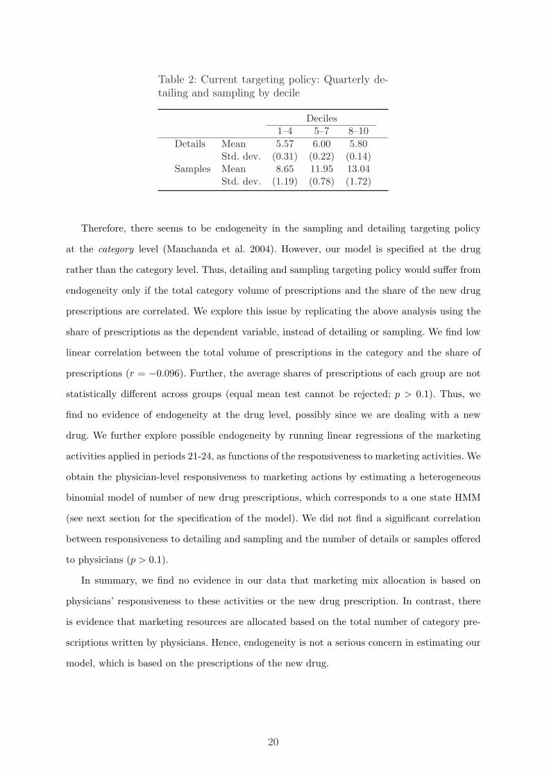
Table 2: Current targeting policy: Quarterly de-tailing and sampling by decile

Deciles1–4 5–7 8–10

Details Mean 5.57 6.00 5.80Std. dev. (0.31) (0.22) (0.14)

Samples Mean 8.65 11.95 13.04Std. dev. (1.19) (0.78) (1.72)

Therefore, there seems to be endogeneity in the sampling and detailing targeting policy

at the category level (Manchanda et al. 2004). However, our model is specified at the drug

rather than the category level. Thus, detailing and sampling targeting policy would suffer from

endogeneity only if the total category volume of prescriptions and the share of the new drug

prescriptions are correlated. We explore this issue by replicating the above analysis using the

share of prescriptions as the dependent variable, instead of detailing or sampling. We find low

linear correlation between the total volume of prescriptions in the category and the share of

prescriptions (r = −0.096). Further, the average shares of prescriptions of each group are not

statistically different across groups (equal mean test cannot be rejected; p > 0.1). Thus, we

find no evidence of endogeneity at the drug level, possibly since we are dealing with a new

drug. We further explore possible endogeneity by running linear regressions of the marketing

activities applied in periods 21-24, as functions of the responsiveness to marketing activities. We

obtain the physician-level responsiveness to marketing actions by estimating a heterogeneous

binomial model of number of new drug prescriptions, which corresponds to a one state HMM

(see next section for the specification of the model). We did not find a significant correlation

between responsiveness to detailing and sampling and the number of details or samples offered

to physicians (p > 0.1).

In summary, we find no evidence in our data that marketing mix allocation is based on

physicians’ responsiveness to these activities or the new drug prescription. In contrast, there

is evidence that marketing resources are allocated based on the total number of category pre-

scriptions written by physicians. Hence, endogeneity is not a serious concern in estimating our

model, which is based on the prescriptions of the new drug.

20

4.4. Model Specification

To parsimoniously model the physician prescription behavior and the effects of detailing and

sampling, we make a few modifications to each one of the three components of the general

HMM described in Section 3.1.

1. Initial state-membership probabilities. Since this is a new drug, we assume that all physi-

cians start at state 1, which corresponds to the lowest prescription-behavior state, in the

first month.11 Thus,

πi = [πi1, πi2, . . . , πiS ] = [1, 0, . . . , 0]. (13)

2. Markov chain transition matrices. Our data set includes two marketing actions that may

have long-term effects on the physicians’ prescription behavior and should be included

in the transition matrix: detailing and sampling. Accordingly, the vector of marketing

actions in Equations (2) and (3) includes:

zit = [f(Detailingit), f(Samplingit)], (14)

where Detailingit and Samplingit correspond to the number of details and samples that

physician i receives in month t, and f(x) = ln(x+1)−µσ , where µ = mean(ln(x + 1)), and

σ = std(ln(x + 1)). We log transform detailing and sampling to capture the potentially

diminishing returns of their effectiveness (Gonul et al. 2001; Manchanda and Chintagunta

2004). We normalize these variables to ensure a proper identification of the prescription-

behavior states (as we describe later).

3. Conditional choice behavior. This component of the HMM captures the physicians’ pre-

scription behavior conditional on their state. We model the prescription behavior Yit as

the number of prescriptions written by physician i in month t. To account for category

demand, let Wit be the total number of new prescriptions in the category written by

physician i in month t. Then, the number of prescriptions of the new drug Yit has a bino-

mial distribution with parameters pist and Wit, where pist is the probability of physician

i prescribing the new drug in month t. That is,

Pist(Yit = yit|Xit = s, zit) =(

Wit

yit

)pyit

ist(1− pist)Wit−yit . (15)

11The more general specification of estimating the vector πi provides no significant improvement in fit.

21

To capture the short-term impact of marketing actions on share-of-prescriptions, we define:

pist =exp(α0

s + α′iszit)1 + exp(α0

s + α′iszit)(16)

where α0s is the intrinsic probability of prescribing given state s, and zit includes the

transformed Detailingit and Samplingit variables in Equation (14). To ensure the iden-

tification of the states we impose that the choice probabilities in the binomial model

are non-decreasing in the behavioral states. We impose this restriction at the mean of

the vector of covariates, zit, such that α01 ≤ · · · ≤ α0

S is imposed by α01 = α0

1; α0s =

α0s−1 + exp(α0

s)∀ s = 2, . . . , S.

There are several advantages for using the binomial distribution in the current ap-

plication. First, since we do not model patients’ demand explicitly, by accounting for

category prescriptions we control for variation in patients’ demand in the entire category.

Second, category prescriptions help to control for any seasonal or time-specific effects that

may affect the market or the specific physician. Third, the binomial distribution can easily

handle extreme values of share-of-prescriptions observed in our data (0 and 1).

Plugging Equations (13), (15), and (16) into Equation (7) produces the likelihood of ob-

serving a sequence of prescriptions.

4.5. Model Estimation

In this section we briefly discuss the procedure we use to estimate our model. To ensure that

cross individual heterogeneity is distinguished from time dynamics we specify the HMM pa-

rameters at the individual level.12 We estimate the transition matrix parameters and the state

dependent choice parameters described in Equations (2)–(4) and (13)–(16) using the joint like-

lihood function in Equation (7). We define Φ ={

α0s

}S

s=1as the set of fixed-effect parameters

and θi ={

τis1, . . . , τisS−1, ρis, αis

}S

s=1as the set of random-effect parameters. We estimate the

random- and fixed-effect HMM parameters using a hierarchical Bayes Markov Chain Monte

Carlo (MCMC) procedure (Rossi et al. 2005).

In the hierarchical Bayes procedure, we recursively draw from the conditional distribution

of each parameter. Given that the conditional posterior distributions of θi and Φ do not have

12For practical purposes we assume that the intrinsic conditional probabilities of prescribing α0s in Equation (16) do

not vary across physicians. This helps us to interpret and compare physicians’ behavior across states in a normalizedway.

22

a closed form, we employ a Gibbs sampler and a random-walk Metropolis-Hastings procedure

to draw candidates and obtain the conditional distribution for each of the parameters. Unlike

HMM Bayesian estimation methods that augment the latent state membership (Djuric and

Chun 2002; Kim and Nelson 1999; Moon et al. 2007; Scott 2002), we follow Netzer et al. (2007)

and use the Bayesian approach to estimate directly the likelihood function in Equation (7) with

random- and fixed-effect parameters. Due to the intrinsic autocorrelation of the HMM, which

leads to autocorrelation between successive draws of the MCMC chain, we use the adaptive

procedure proposed by Atchade (2006) which improves convergence and mixing properties. See

Appendix B for a further description of the MCMC estimation procedure and the prior and

posterior distributions of the HMM.

We use the first 20 months of data to estimate the model and the last four months for

validation purposes. We ran the hierarchical Bayes estimation for 300,000 iterations. The first

200,000 iterations were used as a “burn-in” period and the last 100,000 iterations were used to

estimate the conditional posterior distributions. Convergence was assessed by running multiple

parallel chains following Gelman and Rubin’s criterion (Gelman and Rubin 1992).

4.6. Results and Marketing Implications

4.6.1. Model Selection. The number of states could be estimated from data or specified a

priori based on theoretical grounds. We take the former approach and treat the number of states

as a parameter to be estimated to optimize goodness of fit criteria. Specifically, to choose the

number of states (S) we used the marginal log density (MLL), the deviance information criterion

(DIC), the log Bayes factor (Log BF), and the validation log-likelihood. All these measures are

calculated from the output of the Metropolis-Hastings sampler. The MLL is calculated using

the harmonic mean of the individual likelihoods across iterations (Newton and Raftery 1994).

A one-state model corresponds to a binomial model without dynamics, which is characterized

by equations (15) and (16).

The results in Table 3 suggest selecting a three-state model. This model maximizes the

marginal log density, shows a favorable log Bayes factor in comparison to the models with two

and four states, minimizes the DIC value, and shows the best predictive fit (highest validation

log-likelihood) for the validation periods (periods 21-24).13

13We also tested a four-state model with an absorbing no prescription (“defected”) state. The fit criteria for thismodel are: MLL = -8517, DIC/2 = 8840, Validation log-likelihood = -2195. Therefore, a model where physicians canmove to a “defected” state is rejected in favor of a model with three states. The constrained model is also rejected

23

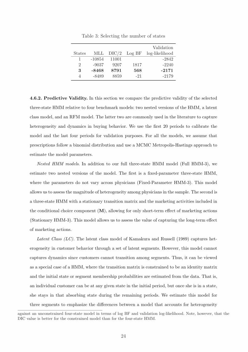
Table 3: Selecting the number of states

ValidationStates MLL DIC/2 Log BF log-likelihood

1 -10854 11001 -28422 -9037 9207 1817 -22403 -8468 8791 568 -21714 -8489 8859 -21 -2179

4.6.2. Predictive Validity. In this section we compare the predictive validity of the selected

three-state HMM relative to four benchmark models: two nested versions of the HMM, a latent

class model, and an RFM model. The latter two are commonly used in the literature to capture

heterogeneity and dynamics in buying behavior. We use the first 20 periods to calibrate the

model and the last four periods for validation purposes. For all the models, we assume that

prescriptions follow a binomial distribution and use a MCMC Metropolis-Hastings approach to

estimate the model parameters.

Nested HMM models. In addition to our full three-state HMM model (Full HMM-3), we

estimate two nested versions of the model. The first is a fixed-parameter three-state HMM,

where the parameters do not vary across physicians (Fixed-Parameter HMM-3). This model

allows us to assess the magnitude of heterogeneity among physicians in the sample. The second is

a three-state HMM with a stationary transition matrix and the marketing activities included in

the conditional choice component (M), allowing for only short-term effect of marketing actions

(Stationary HMM-3). This model allows us to assess the value of capturing the long-term effect

of marketing actions.

Latent Class (LC). The latent class model of Kamakura and Russell (1989) captures het-

erogeneity in customer behavior through a set of latent segments. However, this model cannot

captures dynamics since customers cannot transition among segments. Thus, it can be viewed

as a special case of a HMM, where the transition matrix is constrained to be an identity matrix

and the initial state or segment membership probabilities are estimated from the data. That is,

an individual customer can be at any given state in the initial period, but once she is in a state,

she stays in that absorbing state during the remaining periods. We estimate this model for

three segments to emphasize the differences between a model that accounts for heterogeneity

against an unconstrained four-state model in terms of log BF and validation log-likelihood. Note, however, that theDIC value is better for the constrained model than for the four-state HMM.

24

only and a model that accounts for both heterogeneity and dynamics.

RFM model. One of the models most commonly used to capture dynamics and manage

the firm’s customer base is the recency, frequency and monetary value model (Bitran and

Mondschein 1996, Colombo and Jiang 1999, Pfeifer and Carraway 2000). We construct the RFM

variables as follows: recency corresponds to the number of months since the last prescription,

frequency corresponds to the average incidence of prescription up to the current time period,

and monetary value is captured by the monthly average quantity of prescriptions of the new

drug up to the current time period. These variables are defined at the physician level and are

updated every month. Additionally, we add the transformed detailing and sampling variables

to account for the effect of marketing activities.

We use the cross-validation method to asses the predictive validity of the alternative models.

In this method, the predictive distribution of the holdout observations is derived to examine

whether the actual data points fall in regions of reasonably high density. If we partition the

data as y = [yout, y−out], where yout is the set of “holdout” observations to be removed, and

y−out describes the “calibration” set of observations, the density of the posterior predictive

distribution can be written as:

p(yout|y−out) =∫

Θp(yout|Θ)p(Θ|y−out)dΘ,

where Θ is the vector of the model’s parameters.

One way of assessing the predictive validity is to compute the conditional predictive ordi-

nate (CPO) (Geisser 1993; Gelfand and Dey 1994; Manchanda and Chintagunta 2004). The

logarithm of the CPO for a given model, or the validation log-likelihood, calculated via MCMC

methods, is given by:

log[CPO] =No∑

out=1

log[p(yout|y−out)] =No∑

out=1

log

(1

Nk

Nk∑

k=1

p(yout|Θk)

),

where No is the number of observations in the validation set, Nk is the number of MCMC

iterations, and p(yout|Θk) is the likelihood for the validation period.

Based on the validation log-likelihood and the RMSE criteria (see Table 4), the selected

three-state HMM (Full HMM-3) predicted the holdout prescription data best. Moreover, the

superior fit and prediction of the dynamic fixed-parameter HMM (Fixed-Parameter HMM-

25

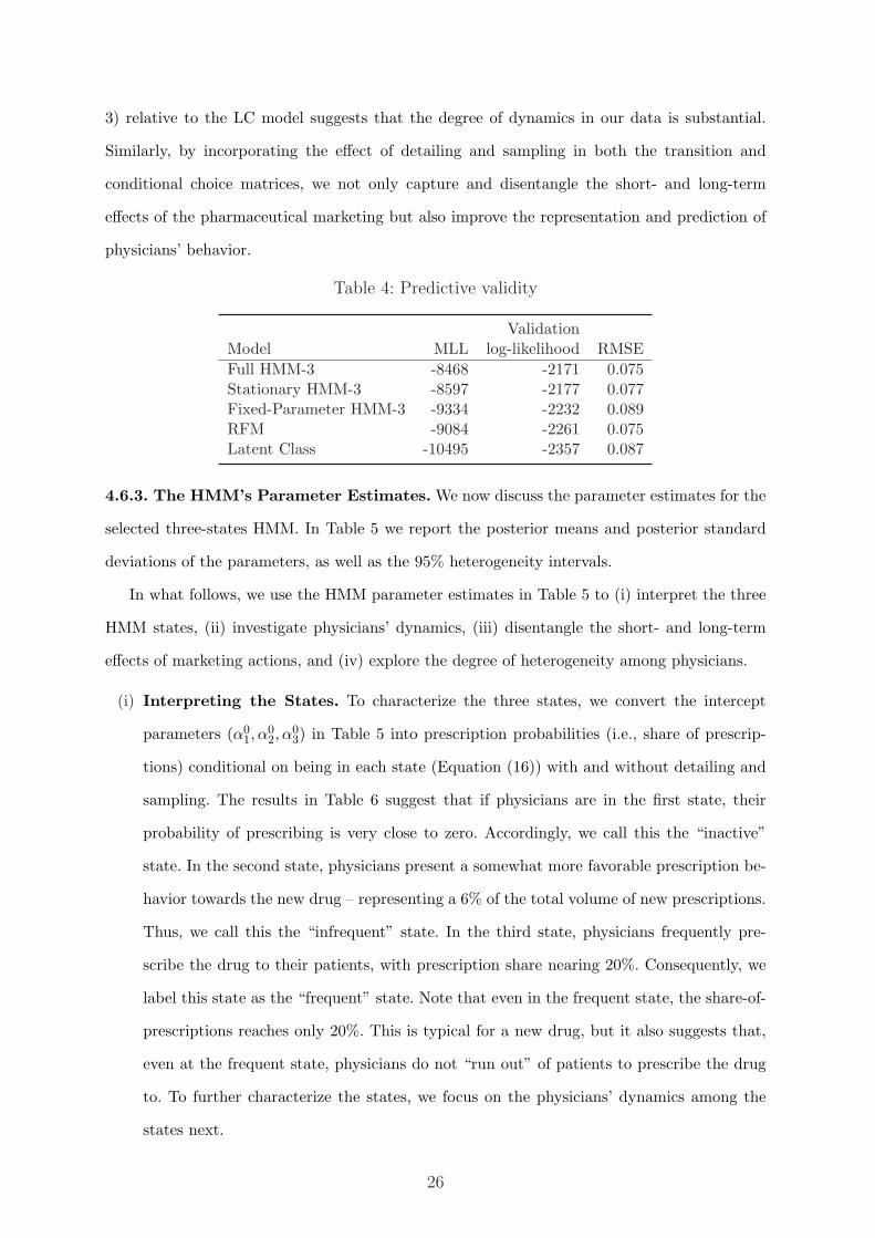
3) relative to the LC model suggests that the degree of dynamics in our data is substantial.

Similarly, by incorporating the effect of detailing and sampling in both the transition and

conditional choice matrices, we not only capture and disentangle the short- and long-term

effects of the pharmaceutical marketing but also improve the representation and prediction of

physicians’ behavior.

Table 4: Predictive validity

ValidationModel MLL log-likelihood RMSEFull HMM-3 -8468 -2171 0.075Stationary HMM-3 -8597 -2177 0.077Fixed-Parameter HMM-3 -9334 -2232 0.089RFM -9084 -2261 0.075Latent Class -10495 -2357 0.087

4.6.3. The HMM’s Parameter Estimates. We now discuss the parameter estimates for the

selected three-states HMM. In Table 5 we report the posterior means and posterior standard

deviations of the parameters, as well as the 95% heterogeneity intervals.

In what follows, we use the HMM parameter estimates in Table 5 to (i) interpret the three

HMM states, (ii) investigate physicians’ dynamics, (iii) disentangle the short- and long-term

effects of marketing actions, and (iv) explore the degree of heterogeneity among physicians.

(i) Interpreting the States. To characterize the three states, we convert the intercept

parameters (α01, α

02, α

03) in Table 5 into prescription probabilities (i.e., share of prescrip-

tions) conditional on being in each state (Equation (16)) with and without detailing and

sampling. The results in Table 6 suggest that if physicians are in the first state, their

probability of prescribing is very close to zero. Accordingly, we call this the “inactive”

state. In the second state, physicians present a somewhat more favorable prescription be-

havior towards the new drug – representing a 6% of the total volume of new prescriptions.

Thus, we call this the “infrequent” state. In the third state, physicians frequently pre-

scribe the drug to their patients, with prescription share nearing 20%. Consequently, we

label this state as the “frequent” state. Note that even in the frequent state, the share-of-

prescriptions reaches only 20%. This is typical for a new drug, but it also suggests that,

even at the frequent state, physicians do not “run out” of patients to prescribe the drug

to. To further characterize the states, we focus on the physicians’ dynamics among the

states next.

26

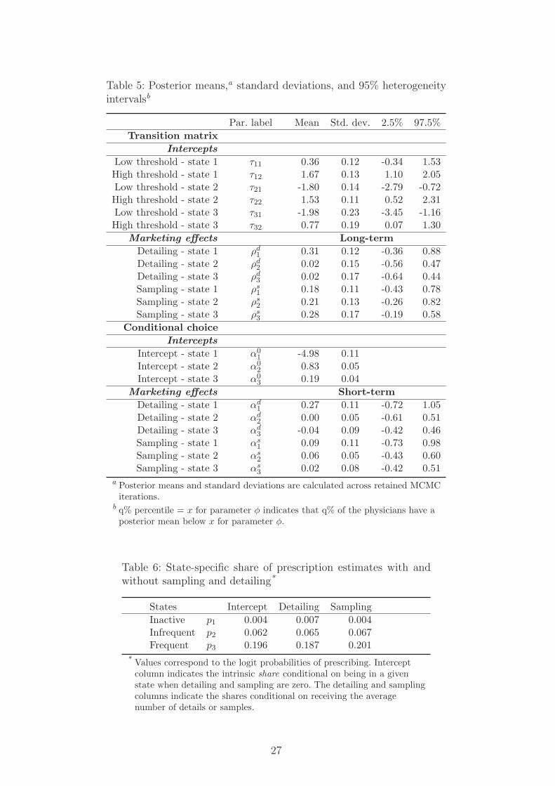
Table 5: Posterior means,a standard deviations, and 95% heterogeneityintervalsb

Par. label Mean Std. dev. 2.5% 97.5%Transition matrix

Intercepts

Low threshold - state 1 τ11 0.36 0.12 -0.34 1.53High threshold - state 1 τ12 1.67 0.13 1.10 2.05Low threshold - state 2 τ21 -1.80 0.14 -2.79 -0.72High threshold - state 2 τ22 1.53 0.11 0.52 2.31Low threshold - state 3 τ31 -1.98 0.23 -3.45 -1.16High threshold - state 3 τ32 0.77 0.19 0.07 1.30

Marketing effects Long-termDetailing - state 1 ρd

1 0.31 0.12 -0.36 0.88Detailing - state 2 ρd

2 0.02 0.15 -0.56 0.47Detailing - state 3 ρd

3 0.02 0.17 -0.64 0.44Sampling - state 1 ρs

1 0.18 0.11 -0.43 0.78Sampling - state 2 ρs

2 0.21 0.13 -0.26 0.82Sampling - state 3 ρs

3 0.28 0.17 -0.19 0.58Conditional choice

Intercepts

Intercept - state 1 α01 -4.98 0.11

Intercept - state 2 α02 0.83 0.05

Intercept - state 3 α03 0.19 0.04

Marketing effects Short-termDetailing - state 1 αd

1 0.27 0.11 -0.72 1.05Detailing - state 2 αd

2 0.00 0.05 -0.61 0.51Detailing - state 3 αd

3 -0.04 0.09 -0.42 0.46Sampling - state 1 αs

1 0.09 0.11 -0.73 0.98Sampling - state 2 αs

2 0.06 0.05 -0.43 0.60Sampling - state 3 αs

3 0.02 0.08 -0.42 0.51a Posterior means and standard deviations are calculated across retained MCMC

iterations.b q% percentile = x for parameter φ indicates that q% of the physicians have a

posterior mean below x for parameter φ.

Table 6: State-specific share of prescription estimates with andwithout sampling and detailing*

States Intercept Detailing SamplingInactive p1 0.004 0.007 0.004Infrequent p2 0.062 0.065 0.067Frequent p3 0.196 0.187 0.201

* Values correspond to the logit probabilities of prescribing. Interceptcolumn indicates the intrinsic share conditional on being in a givenstate when detailing and sampling are zero. The detailing and samplingcolumns indicate the shares conditional on receiving the averagenumber of details or samples.

27

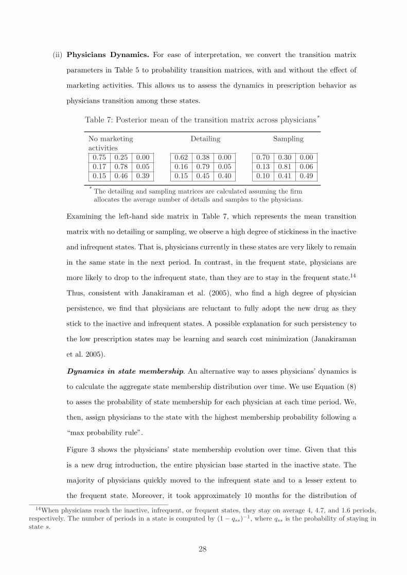
(ii) Physicians Dynamics. For ease of interpretation, we convert the transition matrix

parameters in Table 5 to probability transition matrices, with and without the effect of

marketing activities. This allows us to assess the dynamics in prescription behavior as

physicians transition among these states.

Table 7: Posterior mean of the transition matrix across physicians*

No marketing Detailing Samplingactivities0.75 0.25 0.00 0.62 0.38 0.00 0.70 0.30 0.000.17 0.78 0.05 0.16 0.79 0.05 0.13 0.81 0.060.15 0.46 0.39 0.15 0.45 0.40 0.10 0.41 0.49

* The detailing and sampling matrices are calculated assuming the firmallocates the average number of details and samples to the physicians.

Examining the left-hand side matrix in Table 7, which represents the mean transition

matrix with no detailing or sampling, we observe a high degree of stickiness in the inactive

and infrequent states. That is, physicians currently in these states are very likely to remain

in the same state in the next period. In contrast, in the frequent state, physicians are

more likely to drop to the infrequent state, than they are to stay in the frequent state.14

Thus, consistent with Janakiraman et al. (2005), who find a high degree of physician

persistence, we find that physicians are reluctant to fully adopt the new drug as they

stick to the inactive and infrequent states. A possible explanation for such persistency to

the low prescription states may be learning and search cost minimization (Janakiraman

et al. 2005).

Dynamics in state membership. An alternative way to asses physicians’ dynamics is

to calculate the aggregate state membership distribution over time. We use Equation (8)

to asses the probability of state membership for each physician at each time period. We,

then, assign physicians to the state with the highest membership probability following a

“max probability rule”.

Figure 3 shows the physicians’ state membership evolution over time. Given that this

is a new drug introduction, the entire physician base started in the inactive state. The

majority of physicians quickly moved to the infrequent state and to a lesser extent to

the frequent state. Moreover, it took approximately 10 months for the distribution of

14When physicians reach the inactive, infrequent, or frequent states, they stay on average 4, 4.7, and 1.6 periods,respectively. The number of periods in a state is computed by (1− qss)−1, where qss is the probability of staying instate s.

28

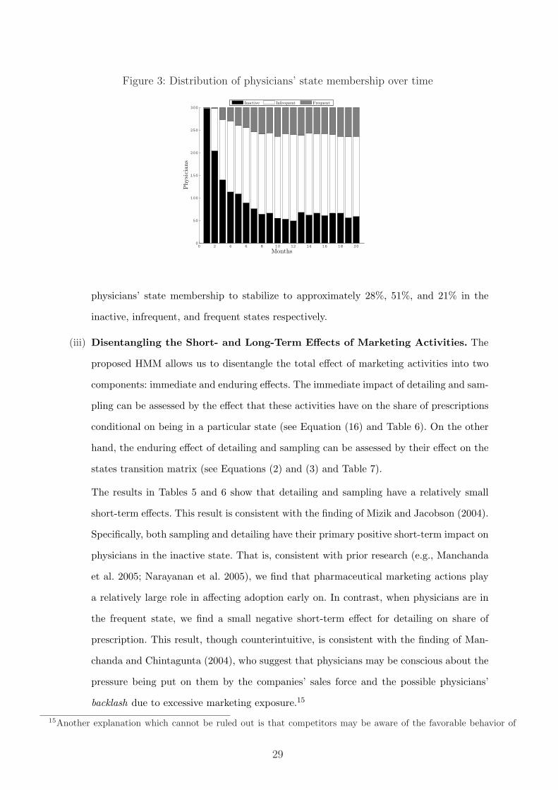
Figure 3: Distribution of physicians’ state membership over time

0 2 4 6 8 10 12 14 16 18 200

50

100

150

200

250

300

Months

Physi

cians

Inactive Infrequent Frequent

physicians’ state membership to stabilize to approximately 28%, 51%, and 21% in the

inactive, infrequent, and frequent states respectively.

(iii) Disentangling the Short- and Long-Term Effects of Marketing Activities. The

proposed HMM allows us to disentangle the total effect of marketing activities into two

components: immediate and enduring effects. The immediate impact of detailing and sam-

pling can be assessed by the effect that these activities have on the share of prescriptions

conditional on being in a particular state (see Equation (16) and Table 6). On the other

hand, the enduring effect of detailing and sampling can be assessed by their effect on the

states transition matrix (see Equations (2) and (3) and Table 7).

The results in Tables 5 and 6 show that detailing and sampling have a relatively small

short-term effects. This result is consistent with the finding of Mizik and Jacobson (2004).

Specifically, both sampling and detailing have their primary positive short-term impact on

physicians in the inactive state. That is, consistent with prior research (e.g., Manchanda

et al. 2005; Narayanan et al. 2005), we find that pharmaceutical marketing actions play

a relatively large role in affecting adoption early on. In contrast, when physicians are in

the frequent state, we find a small negative short-term effect for detailing on share of

prescription. This result, though counterintuitive, is consistent with the finding of Man-

chanda and Chintagunta (2004), who suggest that physicians may be conscious about the

pressure being put on them by the companies’ sales force and the possible physicians’

backlash due to excessive marketing exposure.15

15Another explanation which cannot be ruled out is that competitors may be aware of the favorable behavior of

29

In contrast to the relatively small short-term effects of these marketing activities, detailing

and sampling have significant enduring effects. The results in Table 5 and in the middle

and right matrices in Table 7 show that detailing and sampling have substantial effects in

switching physicians from lower states to higher ones. By comparing the transition matrix

without marketing mix interventions (left side of Table 7), with detailing only (center of

Table 7), and with sampling only (right side of Table 7), we can see that detailing has a

strong effect in moving physicians away from the inactive state. Sampling, on the other

hand, is less effective in moving physicians away from the inactive state, but is more

effective in keeping them in the frequent state. Thus, while detailing may be more useful

as an acquisition tool, sampling is more useful as a retention tool. A possible explanation

for this result is that when physicians are in the inactive state, they are more receptive to

new information about the drug. Then, when they move to the infrequent and frequent

states, there is diminishing return to additional information about the new drug. In the

frequent state, physicians (and their patients) can primarily benefit from receiving free

samples to encourage them to keep on prescribing the new drug.

Detailing and sampling elasticities. To analyze the overall impact of detailing and

sampling, we compute the elasticities of new prescriptions with respect to each marketing

activity. Average elasticities are computed numerically using the formula: ey,x = ∆y/y∆x/x ,

where y corresponds to the average monthly number of new prescriptions and x corre-

sponds to the average monthly number of details or samples.

To compute the increase in prescriptions (∆y), we use the parameter estimates from the

HMM to simulate the effect of targeting one detail or one sample to each physician in the

first month of the simulation (thus, ∆x = 300 = 1 detail (or sample) x 300 physicians).

We first compute the base prescription of the new drug when no details or samples are

allocated to the physicians (y0). Then, we compute the number of prescriptions during the

next 20 months following the targeting of one detail or one sample (y1). Thus, ∆y = y1−y0.

To compute the short-term elasticities, we consider the effect of detailing or sampling in

the first month only; whereas to compute the long-term elasticities, we consider the effect

in the remaining 19 months.

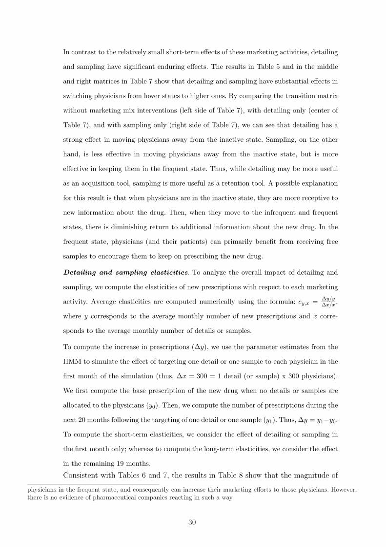
Consistent with Tables 6 and 7, the results in Table 8 show that the magnitude of

physicians in the frequent state, and consequently can increase their marketing efforts to those physicians. However,there is no evidence of pharmaceutical companies reacting in such a way.

30

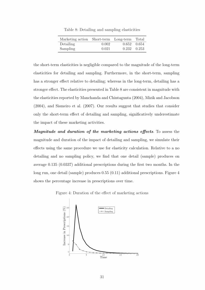
Table 8: Detailing and sampling elasticities

Marketing action Short-term Long-term TotalDetailing 0.002 0.652 0.654Sampling 0.021 0.232 0.253

the short-term elasticities is negligible compared to the magnitude of the long-term

elasticities for detailing and sampling. Furthermore, in the short-term, sampling

has a stronger effect relative to detailing; whereas in the long-term, detailing has a

stronger effect. The elasticities presented in Table 8 are consistent in magnitude with

the elasticities reported by Manchanda and Chintagunta (2004), Mizik and Jacobson

(2004), and Sismeiro et al. (2007). Our results suggest that studies that consider

only the short-term effect of detailing and sampling, significatively underestimate

the impact of these marketing activities.

Magnitude and duration of the marketing actions effects. To assess the

magnitude and duration of the impact of detailing and sampling, we simulate their

effects using the same procedure we use for elasticity calculation. Relative to a no

detailing and no sampling policy, we find that one detail (sample) produces on

average 0.135 (0.0337) additional prescriptions during the first two months. In the

long run, one detail (sample) produces 0.55 (0.11) additional prescriptions. Figure 4

shows the percentage increase in prescriptions over time.

Figure 4: Duration of the effect of marketing actions

0 5 10 15 20

1

5

10

15

20

25

Time

Incr

ease

inP

resc

ription

s(%

)

Detailing

Sampling

31

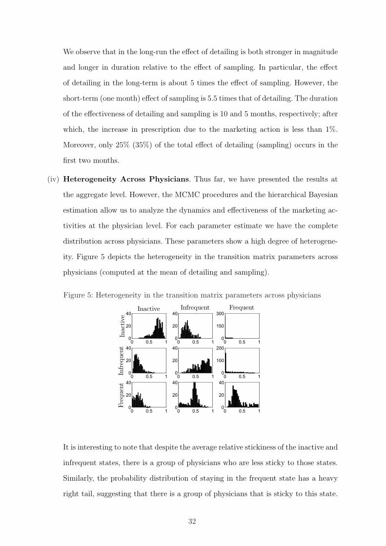
We observe that in the long-run the effect of detailing is both stronger in magnitude

and longer in duration relative to the effect of sampling. In particular, the effect

of detailing in the long-term is about 5 times the effect of sampling. However, the

short-term (one month) effect of sampling is 5.5 times that of detailing. The duration

of the effectiveness of detailing and sampling is 10 and 5 months, respectively; after

which, the increase in prescription due to the marketing action is less than 1%.

Moreover, only 25% (35%) of the total effect of detailing (sampling) occurs in the

first two months.

(iv) Heterogeneity Across Physicians. Thus far, we have presented the results at

the aggregate level. However, the MCMC procedures and the hierarchical Bayesian

estimation allow us to analyze the dynamics and effectiveness of the marketing ac-

tivities at the physician level. For each parameter estimate we have the complete

distribution across physicians. These parameters show a high degree of heterogene-

ity. Figure 5 depicts the heterogeneity in the transition matrix parameters across

physicians (computed at the mean of detailing and sampling).

Figure 5: Heterogeneity in the transition matrix parameters across physicians

0 0.5 10

20

40

Inact

ive

Inactive

0 0.5 10

20

40

Infrequent

0 0.5 10

150

300

Frequent

0 0.5 10

20

40

Infr

equen

t

0 0.5 10

20

40

0 0.5 10

100

200

0 0.5 10

20

40

Fre

quen

t

0 0.5 10

20

40

0 0.5 10

20

40

It is interesting to note that despite the average relative stickiness of the inactive and

infrequent states, there is a group of physicians who are less sticky to those states.

Similarly, the probability distribution of staying in the frequent state has a heavy

right tail, suggesting that there is a group of physicians that is sticky to this state.

32

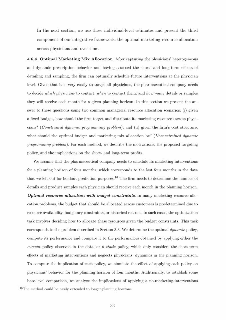
In the next section, we use these individual-level estimates and present the third

component of our integrative framework: the optimal marketing resource allocation

across physicians and over time.

4.6.4. Optimal Marketing Mix Allocation. After capturing the physicians’ heterogeneous

and dynamic prescription behavior and having assessed the short- and long-term effects of

detailing and sampling, the firm can optimally schedule future interventions at the physician

level. Given that it is very costly to target all physicians, the pharmaceutical company needs

to decide which physicians to contact, when to contact them, and how many details or samples

they will receive each month for a given planning horizon. In this section we present the an-

swer to these questions using two common managerial resource allocation scenarios: (i) given

a fixed budget, how should the firm target and distribute its marketing resources across physi-

cians? (Constrained dynamic programming problem); and (ii) given the firm’s cost structure,

what should the optimal budget and marketing mix allocation be? (Unconstrained dynamic

programming problem). For each method, we describe the motivations, the proposed targeting

policy, and the implications on the short- and long-term profits.

We assume that the pharmaceutical company needs to schedule its marketing interventions

for a planning horizon of four months, which corresponds to the last four months in the data

that we left out for holdout prediction purposes.16 The firm needs to determine the number of

details and product samples each physician should receive each month in the planning horizon.

Optimal resource allocation with budget constraints. In many marketing resource allo-

cation problems, the budget that should be allocated across customers is predetermined due to

resource availability, budgetary constraints, or historical reasons. In such cases, the optimization

task involves deciding how to allocate these resources given the budget constraints. This task

corresponds to the problem described in Section 3.3. We determine the optimal dynamic policy,

compute its performance and compare it to the performances obtained by applying either the

current policy observed in the data; or a static policy, which only considers the short-term

effects of marketing interventions and neglects physicians’ dynamics in the planning horizon.

To compute the implication of each policy, we simulate the effect of applying each policy on

physicians’ behavior for the planning horizon of four months. Additionally, to establish some

base-level comparison, we analyze the implications of applying a no-marketing-interventions

16The method could be easily extended to longer planning horizons.

33

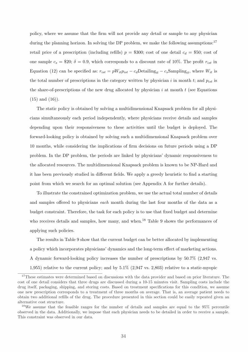
policy, where we assume that the firm will not provide any detail or sample to any physician

during the planning horizon. In solving the DP problem, we make the following assumptions:17

retail price of a prescription (including refills) p = $300; cost of one detail cd = $50; cost of

one sample cs = $20; δ = 0.9, which corresponds to a discount rate of 10%. The profit rist in

Equation (12) can be specified as: rist = pWitpist − cdDetailingit − csSamplingit, where Wit is

the total number of prescriptions in the category written by physician i in month t; and pist is

the share-of-prescriptions of the new drug allocated by physician i at month t (see Equations

(15) and (16)).

The static policy is obtained by solving a multidimensional Knapsack problem for all physi-

cians simultaneously each period independently, where physicians receive details and samples

depending upon their responsiveness to these activities until the budget is deployed. The

forward-looking policy is obtained by solving such a multidimensional Knapsack problem over

10 months, while considering the implications of firm decisions on future periods using a DP

problem. In the DP problem, the periods are linked by physicians’ dynamic responsiveness to

the allocated resources. The multidimensional Knapsack problem is known to be NP-Hard and

it has been previously studied in different fields. We apply a greedy heuristic to find a starting

point from which we search for an optimal solution (see Appendix A for further details).

To illustrate the constrained optimization problem, we use the actual total number of details

and samples offered to physicians each month during the last four months of the data as a

budget constraint. Therefore, the task for each policy is to use that fixed budget and determine

who receives details and samples, how many, and when.18 Table 9 shows the performances of

applying such policies.

The results in Table 9 show that the current budget can be better allocated by implementing

a policy which incorporates physicians’ dynamics and the long-term effect of marketing actions.

A dynamic forward-looking policy increases the number of prescriptions by 50.7% (2,947 vs.

1,955) relative to the current policy; and by 5.1% (2,947 vs. 2,803) relative to a static-myopic

17These estimates were determined based on discussions with the data provider and based on prior literature. Thecost of one detail considers that three drugs are discussed during a 10-15 minutes visit. Sampling costs include thedrug itself, packaging, shipping, and storing costs. Based on treatment specifications for this condition, we assumeone new prescription corresponds to a treatment of three months on average. That is, an average patient needs toobtain two additional refills of the drug. The procedure presented in this section could be easily repeated given analternative cost structure.

18We assume that the feasible ranges for the number of details and samples are equal to the 95% percentileobserved in the data. Additionally, we impose that each physician needs to be detailed in order to receive a sample.This constraint was observed in our data.

34

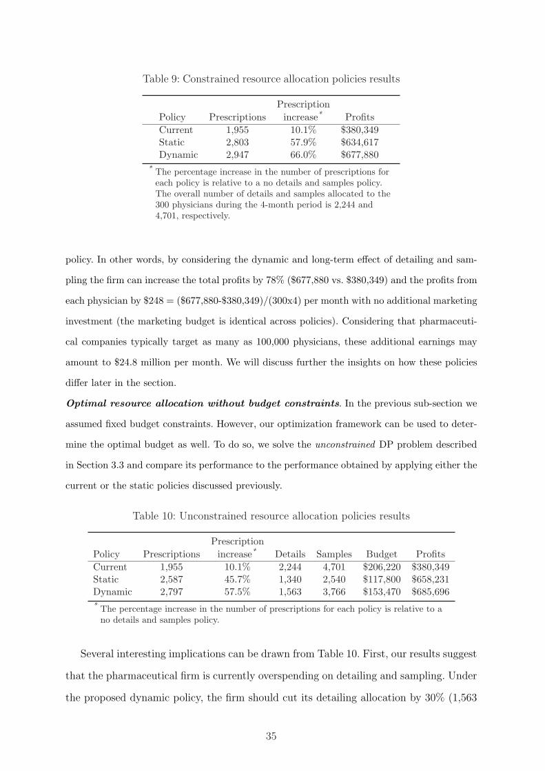
Table 9: Constrained resource allocation policies results

PrescriptionPolicy Prescriptions increase* ProfitsCurrent 1,955 10.1% $380,349Static 2,803 57.9% $634,617Dynamic 2,947 66.0% $677,880

* The percentage increase in the number of prescriptions foreach policy is relative to a no details and samples policy.The overall number of details and samples allocated to the300 physicians during the 4-month period is 2,244 and4,701, respectively.

policy. In other words, by considering the dynamic and long-term effect of detailing and sam-

pling the firm can increase the total profits by 78% ($677,880 vs. $380,349) and the profits from

each physician by $248 = ($677,880-$380,349)/(300x4) per month with no additional marketing

investment (the marketing budget is identical across policies). Considering that pharmaceuti-

cal companies typically target as many as 100,000 physicians, these additional earnings may

amount to $24.8 million per month. We will discuss further the insights on how these policies

differ later in the section.

Optimal resource allocation without budget constraints. In the previous sub-section we

assumed fixed budget constraints. However, our optimization framework can be used to deter-

mine the optimal budget as well. To do so, we solve the unconstrained DP problem described

in Section 3.3 and compare its performance to the performance obtained by applying either the

current or the static policies discussed previously.

Table 10: Unconstrained resource allocation policies results

PrescriptionPolicy Prescriptions increase* Details Samples Budget ProfitsCurrent 1,955 10.1% 2,244 4,701 $206,220 $380,349Static 2,587 45.7% 1,340 2,540 $117,800 $658,231Dynamic 2,797 57.5% 1,563 3,766 $153,470 $685,696* The percentage increase in the number of prescriptions for each policy is relative to a

no details and samples policy.

Several interesting implications can be drawn from Table 10. First, our results suggest

that the pharmaceutical firm is currently overspending on detailing and sampling. Under

the proposed dynamic policy, the firm should cut its detailing allocation by 30% (1,563

35

vs. 2,244), its sampling allocation by 20% (3,766 vs. 4,701), and its overall spending by

26% ($153,470 vs. $206,220). These results are directionally consistent with the finding

of Mizik and Jacobson (2004). Second, despite the 26% cut in spending on marketing

activities, the firm can generate 47.4% (57.5% vs. 10.1%) more prescriptions using the

dynamic policy instead of the current policy, generating an additional $305,347 in profits

from our sample of 300 physicians over a period of four months. The increase in pre-

scription and the decrease in marketing spending lead to an increase of 80% (685,696 vs.

380,349) in profitability relative to the current policy. The optimal budget, then, is about

$128 = $153,470/(300x4) per physician per month ($91 on details and $37 on samples).

Third, a static policy underestimates the overall effect of detailing and sampling as it

only incorporates their short-term effect. As a result, it allocates much less details and

samples to physicians compared to the other policies.

The results of these resource allocation analyzes highlight the possibly substantial

financial implications of simultaneously capturing the dynamics in consumer behavior

and the long-term effect of marketing actions in marketing mix allocation.

Targeting, resource allocation, and timing implications. The optimization ana-

lysis described above suggests that using the dynamic policy, which takes advantage of

the dynamics in prescription behavior and the enduring effect of marketing activities,

the firm can significatively increase the return on marketing investments. To further un-

derstand the drivers of the improved performance of the proposed policy, we investigate

the differences among the policies in terms of: who is being targeted, how the resources

are allocated, and when these resources are distributed across physicians. As the results

in Table 11 suggest, the current, dynamic constrained, and dynamic unconstrained poli-

cies, allocate similar number of details and samples to targeted physicians. However, the

current policy targets a higher percentage of physicians (85%) than the dynamic con-

strained (60%) and dynamic unconstrained (50%) policies. Furthermore, the overlap in

the physicians targeted by the two dynamic policies is very high (over 90%).

Given the congruency between the two dynamic policies, we compare only the current

policy to the dynamic unconstrained policy. We compare these policies in terms of: (i)

targeted physicians, (ii) allocated resources, and (iii) timing of targeting.

36

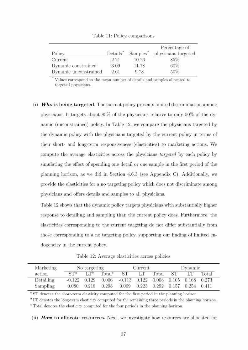
Table 11: Policy comparisons

Percentage ofPolicy Details* Samples* physicians targetedCurrent 2.21 10.26 85%Dynamic constrained 3.09 11.78 60%Dynamic unconstrained 2.61 9.78 50%* Values correspond to the mean number of details and samples allocated to

targeted physicians.

(i) Who is being targeted. The current policy presents limited discrimination among

physicians. It targets about 85% of the physicians relative to only 50% of the dy-

namic (unconstrained) policy. In Table 12, we compare the physicians targeted by

the dynamic policy with the physicians targeted by the current policy in terms of

their short- and long-term responsiveness (elasticities) to marketing actions. We

compute the average elasticities across the physicians targeted by each policy by

simulating the effect of spending one detail or one sample in the first period of the

planning horizon, as we did in Section 4.6.3 (see Appendix C). Additionally, we

provide the elasticities for a no targeting policy which does not discriminate among

physicians and offers details and samples to all physicians.

Table 12 shows that the dynamic policy targets physicians with substantially higher

response to detailing and sampling than the current policy does. Furthermore, the

elasticities corresponding to the current targeting do not differ substantially from

those corresponding to a no targeting policy, supporting our finding of limited en-

dogeneity in the current policy.

Table 12: Average elasticities across policies

Marketing No targeting Current Dynamicaction STa LTb Totalc ST LT Total ST LT TotalDetailing -0.122 0.129 0.006 -0.113 0.122 0.008 0.105 0.168 0.273Sampling 0.080 0.218 0.298 0.069 0.223 0.292 0.157 0.254 0.411

a ST denotes the short-term elasticity computed for the first period in the planning horizon.b LT denotes the long-term elasticity computed for the remaining three periods in the planning horizon.c Total denotes the elasticity computed for the four periods in the planning horizon.

(ii) How to allocate resources. Next, we investigate how resources are allocated for

37

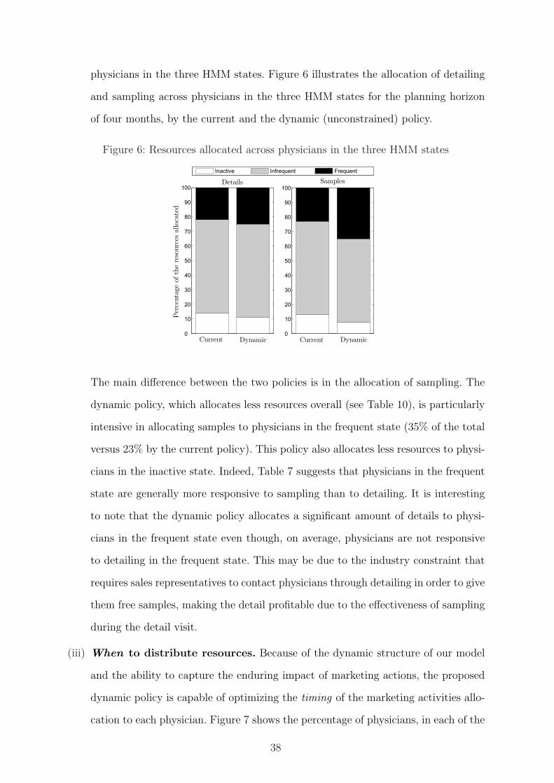
physicians in the three HMM states. Figure 6 illustrates the allocation of detailing

and sampling across physicians in the three HMM states for the planning horizon

of four months, by the current and the dynamic (unconstrained) policy.

Figure 6: Resources allocated across physicians in the three HMM states

0

10

20

30

40

50

60

70

80

90

100

Per

centa

ge

ofth

ere

sourc

esalloca

ted

Details

0

10

20

30

40

50

60

70

80

90

100

Samples

Inactive Infrequent Frequent

Current Dynamic DynamicCurrent

The main difference between the two policies is in the allocation of sampling. The

dynamic policy, which allocates less resources overall (see Table 10), is particularly

intensive in allocating samples to physicians in the frequent state (35% of the total

versus 23% by the current policy). This policy also allocates less resources to physi-

cians in the inactive state. Indeed, Table 7 suggests that physicians in the frequent

state are generally more responsive to sampling than to detailing. It is interesting

to note that the dynamic policy allocates a significant amount of details to physi-

cians in the frequent state even though, on average, physicians are not responsive

to detailing in the frequent state. This may be due to the industry constraint that

requires sales representatives to contact physicians through detailing in order to give

them free samples, making the detail profitable due to the effectiveness of sampling

during the detail visit.

(iii) When to distribute resources. Because of the dynamic structure of our model

and the ability to capture the enduring impact of marketing actions, the proposed

dynamic policy is capable of optimizing the timing of the marketing activities allo-

cation to each physician. Figure 7 shows the percentage of physicians, in each of the

38

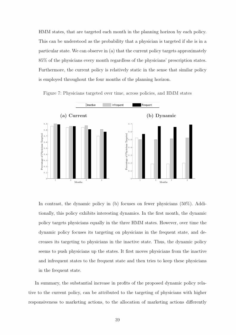
HMM states, that are targeted each month in the planning horizon by each policy.

This can be understood as the probability that a physician is targeted if she is in a

particular state. We can observe in (a) that the current policy targets approximately

85% of the physicians every month regardless of the physicians’ prescription states.

Furthermore, the current policy is relatively static in the sense that similar policy

is employed throughout the four months of the planning horizon.

Figure 7: Physicians targeted over time, across policies, and HMM states

(a) Current (b) Dynamic

1 2 3 40

0.1

0.2

0.3

0.4

0.5

0.6

0.7

0.8

0.9

Months

Per

centa

ge

ofP

hysici

ans

Targ

eted

1 2 3 40

0.1

0.2

0.3

0.4

0.5

0.6

0.7

Months

Per

centa

ge

ofP

hysici

ans

Targ

eted

In contrast, the dynamic policy in (b) focuses on fewer physicians (50%). Addi-

tionally, this policy exhibits interesting dynamics. In the first month, the dynamic

policy targets physicians equally in the three HMM states. However, over time the

dynamic policy focuses its targeting on physicians in the frequent state, and de-

creases its targeting to physicians in the inactive state. Thus, the dynamic policy

seems to push physicians up the states. It first moves physicians from the inactive

and infrequent states to the frequent state and then tries to keep these physicians

in the frequent state.

In summary, the substantial increase in profits of the proposed dynamic policy rela-

tive to the current policy, can be attributed to the targeting of physicians with higher

responsiveness to marketing actions, to the allocation of marketing actions differently

39

across physicians based on the physician state of prescription, and to the use of detailing

as an acquisition tool and sampling as a retention tool.

5. Conclusions

Managing customers through marketing mix allocation has a critical impact on firms’

profitability in the long-term. To successfully target marketing interventions at the in-

dividual level, firms need to consider customers’ evolution over time, heterogeneity in

customers’ dynamics and response to marketing mix interventions, and the possibly en-

during effect of these marketing activities.

In this paper, we present an integrative framework to capture the dynamics in cus-

tomer behavior and long-term effect of marketing activities at the individual level. We

subsequently propose a dynamic programming approach to optimize the marketing mix

allocation for long-term profitability. We identify several interesting findings by apply-

ing our modeling framework in the context of a pharmaceutical new drug introduction.

First, we identify three latent prescription-behavior states which characterize physicians’

dynamic behavior. Second for the particular drug studied, both detailing and sampling

have long-term impact on physicians’ prescription behavior. Third, detailing is particu-

larly effective as an acquisition tool, moving physicians from an inactive state, whereas

sampling is mostly effective as a retention tool, keeping physicians in a high prescription-

behavior state. Fourth, sampling has a stronger short-term effect than detailing, but the

latter has a stronger long-term effect. Fifth, we demonstrate that ignoring the dynam-

ics in physician buying behavior and the long-term effects of marketing activities leads

to suboptimal allocation of marketing interventions. Specifically, using a counterfactual

analysis, we demonstrate that our resource allocation approach leads to an increase of

80% in profitability and that the firm should cut its marketing spending by 26%. Finally,

the optimal dynamic allocation of sampling and detailing involves first moving physicians

away from the inactive state to the frequent state and then retaining these physicians in

the frequent state.

We highlight several limitations and directions that future research could explore.

40

First, in this empirical application, we find no evidence of endogeneity in the detailing and

sampling for the specific drug. In general, if endogeneity is present, one could integrate

into our modeling approach a targeting process equation along the lines of Manchanda et

al. (2004). Second, an alternative source of dynamics not considered in this research comes

from the belief that physicians have foresight regarding their prescription-behavior evolu-

tion and the firm’s marketing mix allocation. One could extend our modeling framework

by formulating a structural model of state-dependence with forward-looking behavior

(Erdem and Keane 1996). Given the nature of dynamics in HMMs, this is likely to com-

plicate the modeling approach significatively. Third, similar to many CRM data sets,

our data include no information about competitive marketing efforts. Obtaining such

information would be helpful to describe physicians’ dynamics. Alternatively, one could

use the HMM approach of Moon et al. (2007) to augment the competitive marketing

efforts. Fourth, the proposed framework can be applied to many CRM applications such

as loyalty programs, contractual services, and new product introduction. In these type

of applications, firms need to trade-off between short- and long-term revenues when al-

locating marketing resources at the individual level.

To summarize, firms are engaged in developing marketing initiatives that are aimed at

enhancing the relationship between the customer and the firm, and thus have an enduring

impact on the customer. Optimal targeting and allocation of such marketing activities is

extremely difficult. In this research, we offer a first step in providing marketing managers a

framework for managing customers for long-run profitability through an efficient dynamic

allocation of marketing resources.

41

Appendix A. Algorithm for Solving the Dynamic Programming

Problem

In this Appendix we describe the details of how we solve the Dynamic Programming (DP) problems

of dynamic marketing mix allocation. Following Section 3.3, the firm’s dynamic marketing allocation

problem can be formulated as:

N∑

i=1

V ∗i (Bit) =

N∑

i=1

maxzit

E{ ∞∑

τ=t

δτ−tRiτ

}

=N∑

i=1

maxzit

{ S∑s=1

bit(s) · rist + δ[V ∗i (Bit+1)]

}, (A.1)

subject to

Bit+1 = BitQit ∀i, t (update beliefs)N∑

i=1

zit ≤ At ∀t (marketing budget)

zit ∈ D ∀i, t (marketing actions space),

it is important to note that the state variables in our DP problem (Bit, beliefs about customer i at

time t) are continuous. Therefore, in contrast to problems with a finite number of state points, it is not

possible to solve exactly for V ∗i (Bit) at every state point. Thus, we employ an approximation method.

Specifically, we follow Keane and Wolpin (1994) by using a polynomial approximation for V ∗i (Bit) as

we describe below.

Given that the firm’s beliefs about customers’ membership to the HMM states add up to one,

the second order polynomial19 for V ∗i (Bit) for the three-state HMM problem used in our empirical

application is a function of the beliefs about customer i’s membership to state 1 and 2 only. Specifically:

V ∗i (Bit) = γi0 + γi1bit(1) + γi2b

2it(1) + γi3bit(2) + γi4b

2it(2) + γi5bit(1)bit(2), (A.2)

where bit(s) corresponds to the firm’s belief about customer i’s membership to state s at time t. The

parameters {γij}5j=0 are estimated by OLS regression for each customer i. To obtain the sample of data

points (belief points) for the interpolation, we calculate V ∗i (Bg) on a grid of NG = 100 belief points

different for each customer i but constant over time.20 To reduce the complexity of the optimization

algorithm, we set up the grid by selecting a sample of beliefs only from a “relevant” space of beliefs for

the customer. The relevant space is defined by the firm’s beliefs about customer i’s membership at time

t and the possible transitions for that customer given the range of marketing actions in each period. For

instance, if the firm’s beliefs about customer i’s membership are Bit = [0.8, 0.2, 0]. Then, by allocating

the minimum number of marketing actions to this customer at period t, its beliefs could be updated for

the next period to be Bminit+1 = [1, 0, 0]. On the other extreme, by allocating the maximum number of

marketing actions to this customer at period t, its beliefs could be updated for the next period to be

19One could define a higher order polynomial. However, for our empirical application a higher order polynomial didnot provide significantly better interpolation results.

20Larger NG(NG = 200, 500, and 1, 000) did not provide significant improvement in fit or predictability.

42

Bmaxit+1 = [0.5, 0.3, 0.2], then only beliefs Bit+1 ∈ [Bmin

it+1,Bmaxit+1] will be feasible. We randomly draw NG

i.i.d. of those feasible beliefs.

Having defined the grid over which we calculate the value functions, we next describe the backsolving

method used to solve the DP problems. For ease of exposition, we first describe the algorithm used for

solving the resource allocation with budget constraints problem, and then, the algorithm used for solving

the resource allocation without budget constraints problem.

Optimal Resource Allocation With Budget Constraints. For the following algorithm we assume

a finite horizon T , and a size NG for the random grid of beliefs. Each period t we create a random grid

for customer i, Git = {ξi,t,j}NGj=1, which represents the firm’s beliefs about customer i’s state membership

at time t. In order to solve the DP problem we employ a procedure which consists of backsolving the DP

problem starting from the last period imposing the known budget constraints for that period. We find

the optimal resource allocation across customers for that period (solving a knapsack problem) and, then,

use the estimated value functions V ∗i (BiT ) to run the OLS regression and estimate the γij coefficients in

Equation (A.2) which are used to approximate the value function in the next step. Then, for period T−1,

we use the interpolated V ∗i (BiT ) in order to optimally solve for V ∗

i (BiT−1). We repeat this procedure

up to time 1. At the initial period of the planning horizon, Bi1 correspond to the firm’s beliefs of

customer i’s state membership at the end of the calibration period. Thus, we use these probabilistically

“known” beliefs to forward allocate the marketing resources following the optimal path determined by

the backsolving procedure of the DP algorithm. To further clarify the employed procedure, we present

a description of the algorithm used:21

1. (Backsolving) Last period T

(a) Create the grid of state-space (beliefs) points GiT = {ξi,T,j}NGj=1 ∀i. The entire grid across

customers GT is of size NG x N , where N is the number of customers.

(b) For each set of beliefs g ∈ GT solve a knapsack problem to allocate marketing resources

across customers.

(c) Compute the value function V ∗iTg for each customer i given the optimal solution reached for

grid point g.

(d) Use {V ∗iTg}NG

g=1 as dependent variable in the OLS regression to obtain the γij parameters, and

approximate V ∗iT for any state beliefs.

2. Period t = T − 1, . . . , 2

(a) Create the grid of state-space (beliefs) points Git = {ξi,t,j}NGj=1 ∀i.

(b) For each set of beliefs g ∈ Gt solve a knapsack problem to allocate marketing resources

across physicians considering short- and long-term effects. Use the approximation V ∗it+1, in

the Bellman equation, to compute V ∗it .

(c) Compute the value function V ∗itg for each customer i given the optimal solution reached for

grid point g.

21For illustration purposes and to simplify notation, we write V ∗i (Bit) as V ∗

it in the following description.

43

(d) Run the OLS regression to obtain the γij parameters and approximate V ∗it−1 for any state

beliefs.

(e) Make t = t− 1 and repeat (a)–(d) until t− 1 = 1.

3. Period 1 (forward allocation). Allocate the marketing resources using Bi1, the optimal policy found

for these beliefs, and the approximation V ∗i2 obtained in period 2 using:

Vi1(Bi1) =S∑

s=1

bi1(s)rist + δV ∗i2(Bi2),

and solving the Knapsack problem in Equation (A.1).

After determining the optimal policy for period 1, update beliefs and move to period 2. Repeat

until terminal period T, where by assumption V ∗iT+1 ≡ 0 for all beliefs and customers.

Optimal Resource Allocation Without Budget Constraints. This case is solved similarly to the

constrained case except for two modifications: (i) there is no common budget constrains across customers.

Therefore, the problem is solved independently for each customer; (ii) we solve an infinite DP problem.

We do so, by implementing a value iteration policy, which consists on backsolving the DP problem for a

sufficiently large number of periods and until no major change is observed in the value function for each

individual. Specifically, we backsolve the DP problem until we reach a point where, in going back one

period, the maximum percentage change in the value function across all grid points - which is measured

by the change in the polynomial parameters γij - is less than 0.1%. In our empirical application, the

mean number of time periods (iterations of the value iteration method) required until convergence was

61.9 and the mean R2 of the OLS regression for the interpolation method was 0.99. We generate the

random grid only once for each customer, and keep it until convergence.

Note that this procedure is impractical when there are budget constrains as the ones described

previously, because a DP problem with budget constraints requires solving a knapsack problem across

customers. This would have to be performed for each iteration of the value iteration method, which

usually requires several iterations until convergence.

Dealing With Local Optima. The objective function of the DP problem described above is highly non-

linear in the decision variables. Therefore, any optimization routine is susceptible to find local optima. To

reduce this concern, a few improvements were implemented. For the problem without budget constrains,

we implemented an enumeration algorithm which computes and compares all feasible solutions and

returns the global maximum. Given that this problem is solved individually, this routine is implementable

in reasonable time. For the problem with budget constrains, an enumeration algorithm is infeasible as

the number of feasible solutions is prohibitive (any feasible solution can be implemented in N ! ways,

where N is the number of customers). We therefore implemented a greedy heuristic to find a good

starting point, from which the optimization routine starts searching for an optimal solution. This greedy

heuristic consists on allocating resources iteratively based on the unit increase in the overall objective

function. This allocation is made in decreasing order of improvement until the total budget is deployed.

44

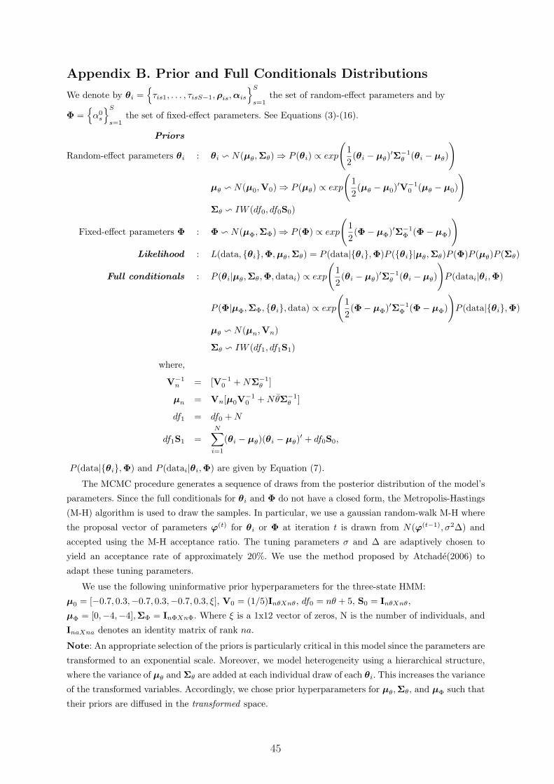
Appendix B. Prior and Full Conditionals Distributions

We denote by θi ={

τis1, . . . , τisS−1,ρis, αis

}S

s=1the set of random-effect parameters and by

Φ ={

α0s

}S

s=1the set of fixed-effect parameters. See Equations (3)-(16).

Priors

Random-effect parameters θi : θi v N(µθ,Σθ) ⇒ P (θi) ∝ exp

(12(θi − µθ)

′Σ−1θ (θi − µθ)

)

µθ v N(µ0,V0) ⇒ P (µθ) ∝ exp

(12(µθ − µ0)

′V−10 (µθ − µ0)

)

Σθ v IW (df0, df0S0)

Fixed-effect parameters Φ : Φ v N(µΦ,ΣΦ) ⇒ P (Φ) ∝ exp

(12(Φ− µΦ)′Σ−1

Φ (Φ− µΦ)

)

Likelihood : L(data, {θi},Φ, µθ,Σθ) = P (data|{θi},Φ)P ({θi}|µθ,Σθ)P (Φ)P (µθ)P (Σθ)

Full conditionals : P (θi|µθ,Σθ,Φ, datai) ∝ exp

(12(θi − µθ)

′Σ−1θ (θi − µθ)

)P (datai|θi,Φ)

P (Φ|µΦ,ΣΦ, {θi},data) ∝ exp

(12(Φ− µΦ)′Σ−1

Φ (Φ− µΦ)

)P (data|{θi},Φ)

µθ v N(µn,Vn)

Σθ v IW (df1, df1S1)

where,

V−1n = [V−1

0 + NΣ−1θ ]

µn = Vn[µ0V−10 + NθΣ−1

θ ]

df1 = df0 + N

df1S1 =N∑

i=1

(θi − µθ)(θi − µθ)′ + df0S0,

P (data|{θi},Φ) and P (datai|θi,Φ) are given by Equation (7).

The MCMC procedure generates a sequence of draws from the posterior distribution of the model’s

parameters. Since the full conditionals for θi and Φ do not have a closed form, the Metropolis-Hastings

(M-H) algorithm is used to draw the samples. In particular, we use a gaussian random-walk M-H where

the proposal vector of parameters ϕ(t) for θi or Φ at iteration t is drawn from N(ϕ(t−1), σ2∆) and

accepted using the M-H acceptance ratio. The tuning parameters σ and ∆ are adaptively chosen to

yield an acceptance rate of approximately 20%. We use the method proposed by Atchade(2006) to

adapt these tuning parameters.

We use the following uninformative prior hyperparameters for the three-state HMM:

µ0 = [−0.7, 0.3,−0.7, 0.3,−0.7, 0.3, ξ], V0 = (1/5)InθXnθ, df0 = nθ + 5, S0 = InθXnθ,

µΦ = [0,−4,−4],ΣΦ = InΦXnΦ. Where ξ is a 1x12 vector of zeros, N is the number of individuals, and

InaXna denotes an identity matrix of rank na.

Note: An appropriate selection of the priors is particularly critical in this model since the parameters are

transformed to an exponential scale. Moreover, we model heterogeneity using a hierarchical structure,

where the variance of µθ and Σθ are added at each individual draw of each θi. This increases the variance

of the transformed variables. Accordingly, we chose prior hyperparameters for µθ,Σθ, and µΦ such that

their priors are diffused in the transformed space.

45

Appendix C. Simulation of the Model

This Appendix describes how we simulate data from the model to compute the magnitude and dura-

tion of marketing effects in Section 4.6.3 and to evaluate the resource allocation policies described in

Section 4.6.4.

Magnitude and Duration of the Marketing Effects. After estimating the parameters of the HMM

we simulate the effects of sending a different number of details and samples to the physicians in the short-

and long-term. We considered 20 months as our planning horizon. We simulate the effects of allocating

no marketing resources in the entire planning horizon and compare it to sending either one detail or

one sample to each customer in the sample in the first period only. That is, 300 details or 300 samples

in period 1 and no details or samples in the next 19 periods. To compare these simulations, we assume

physicians write their expected number of prescriptions given by the binomial model. Furthermore, we

update the membership probabilities (beliefs Bit) in a deterministic manner using Equation (10) in

Section 3.3. (Bit+1 = BitQit). Because in our model detailing and sampling affect both the transition

matrix Qit and the conditional choice matrix Mit, a different sequence of decisions are made based on

differences in physicians’ membership to the prescription-states and their propensity to prescribe the

new drug conditional on being in a state.

Evaluating the Resource Allocation Policies. Having obtained the optimal resource allocation

policies described in Section 4.6.4, we simulate the effects of implementing those policies in the sample

of physicians. The implementation follows analogous steps to the ones described above, with two modifi-

cations: (i) we use a realistic four period planning horizon, which corresponds to the last four periods in

the data (months 21-24), and (ii) the alternative policies imply different marketing resource allocation

throughout the four periods (not only the first period of the planning horizon).

46

References

Atchade, Yves. 2006. An Adaptive Version for the Metropolis Adjusted Langevin Algo-rithm with a Truncated Drift. Methodology and Computing in Applied Probability, 8,235-254.

Aviv, Yossi, Amit Pazgal. 2005. A Partially Observed Markov Decision Process for Dy-namic Pricing. Management Science, 51(9), 1400-1416.

Bates, Andree. 2006. Using ROI Data for Effective Decision Making in PharmaceuticalMarketing. KeywordPharma Expert Review.

Bawa, Kapil, Robert Shoemaker. 1987. The Effects of a Direct Mail Coupon on BrandChoice Behavior. Journal of Marketing Research, 24(4), 370-376.

Bellman, Richard. 1957. Dynamic Programming. Princeton University Press, Princeton.

Bitran, Gabriel, Susana Mondschein. 1996. Mailing Decisions in the Catalog Sales Indus-try. Management Science, 42(9),1364–1381.

Bucklin, Randolph, James Lattin. 1991. A Two-State Model of Purchase Incidence andBrand Choice. Marketing Science, 10(1), 24-39.

Chintagunta, Pradeep, Naufel Vilcassim. 1994. Marketing Investment Decisions in a Dy-namic Duopoly: A Model and Empirical Analysis. International Journal of Researchin Marketing, 11, 287–306.

Colombo, Richard, Weina Jiang. 1999. A Stochastic RFM Model. Journal of InteractiveMarketing, 13(3), 2–12.

Dekimpe, Marnik, Dominique Hanssens. 1995. The Persistence of Marketing Effects onSales. Marketing Science, 14(1), 1-21.

Dekimpe, Marnik, Dominique Hanssens. 1999. Sustained Spending and Persistent Re-sponse: A New Look at Long-Term Marketing Profitability. Journal of MarketingResearch, 36(4), 397-412.

Dekimpe, Marnik, Dominique Hanssens, Vincent Nijs, Jan-Benedict Steenkamp. 2005.Measuring Short- and Long-Run Promotional Effectiveness on Scanner Data usingPersistence Modeling. Applied Stochastic Models in Business and Industry, 21, 409–416.

Djuric, Petar, Joon-Hwa Chun. 2002. An MCMC Sampling Approach to Estimationof Nonstationary Hidden Markov Models. IEEE Transaction on Signal Processing,50(5), 1113–1123.

Du, Rex, Wagner Kamakura. 2006. Household Lifecycles and Lifestyles in America. Jour-nal of Marketing Research, 43(1), 121–132.

Elsner, Ralf, Manfred Krafft, Arnd Huchzermeier. 2004. Optimizing Rhenania’s directmarketing business through dynamic multilevel modeling (DMLM) in a multi-catalog-brand environment. Marketing Science, 23(2), 192-206.

Erdem, Tulim, Susumu Imai, Michael Keane. 2003. A Model of Consumer Brand andQuantity Choice Dynamics under Price Uncertainty. Quantitative Marketing and Eco-

47

nomics, 1(1), 5–64.

Erdem, Tulim, Michael Keane. 1996. Decision-Making under Uncertainty: CapturingDynamic Brand Choice Processes in Turbulent Consumer Goods Markets. MarketingScience, 15(1), 1–20.

Erdem, Tulim, Baohong Sun. 2001. Testing for Choice Dynamics in Panel Data. Journalof Business and Economic Statistics, 19(2), 142–152.

Gatignon, Hubert, Dominique Hanssens. 1987. Modeling Marketing Interaction with Ap-plication to Sales Force Effectiveness. Journal of Marketing Research, 24(3), 247–257.

Geisser, Seymour. 1993. Predictive Inference: An Introduction. Chapman and Hall, Lon-don.

Gelfand, A., D. Dey. 1994. Bayesian Model Choice: Asymptotics and Exact Calculations.Journal of the Royal Statistical Society, Series B, 56, 501–514.

Gelman, Andrew, Donald Rubin. 1992. Inference from Iterative Simulation Using Mul-tiple Sequences. Statistical Science, 7, 457–511.

Gonul, Fusun, Franklin Carter, Elina Petrova, Kannan Srinivasan. 2001. Promotion ofPrescription Drugs and Its Impact on Physicians Choice Behavior. Journal of Mar-keting, 65(3), 79-90.

Gonul, Fusun, Frenkel Ter Hofstede. 2006. How to Compute Optimal Catalog MailingDecisions. Marketing Science, 25(1), 65-74.

Gonul, Fusun, Meng Ze Shi. 1998. Optimal Mailing of Catalogs: A New MethodologyUsing Estimable Structural Dynamic Programming Models. Management Science,44(9), 1249-1262.

Greene, William. 1997. Econometric Analysis. Prentice Hall, Third edition.

Guadagni, Peter, John Little. 1983. A Logit Model Scanner Data. Marketing Science,2(3), 203–238.

Heckman, James. 1981. Heterogeneity and State Dependence. In S.Rosen ed. Studies inLabor Markets, Chicago: University of Chicago Press, 91–139.

Janakiraman, Ramkumar, Shantanu Dutta, Catarina Sismeiro, Phil Stern. 2005. AreThey All the Same? Physicians’ Persistence and Its Implications for Marketing Com-munication. Working paper, Tanaka Business School.

Jedidi, Kamel, Carl Mela, Sunil Gupta. 1999. Managing Advertising and Promotion forLong-Run Profitability. Marketing Science, 18(1), 1–22.

Kamakura, Wagner, Gary Russell. 1989. A Probabilistic Choice Model for Market Seg-mentation and Elasticity Structure. Journal of Marketing Research, 26(4), 379–390.

Keane, Michael. 1997. Modeling Heterogeneity and State Dependence in Consumer ChoiceBehavior. Journal of Business and Economic Statistics, 15(3), 310-327.

Keane, Michael, Kenneth Wolpin. 1994. The Solution and Estimation of Discrete ChoiceDynamic Programming Models by Simulation and Interpolation: Monte Carlo Evi-dence. The Review of Economics and Statistics, MIT Press, vol. 76(4), 648–672.

48

Kim, Chang-Jin, Charles Nelson. 1999. State-Space Models with Regime Switching: Clas-sical and Gibbs Sampling Approaches with Applications. M.I.T. Press, Cambridge,Massachusetts.

Lewis, Michael. 2005. A Dynamic Programming Approach to Customer RelationshipPricing. Management Science, 51(6),986–994.

Liechty, John, Michel Wedel, Rik Pieters. 2003. The Representation of Local and GlobalScanpaths in Eye Movements Through Bayesian Hidden Markov Models. Psychome-trika, 68(4), 519–541.

Lovejoy, William. 1991. Computationally Feasible Bounds for Partially Observed MarkovDecision Processes. Operations Research, 39(1), 162-175.

Manchanda, Puneet, Pradeep Chintagunta. 2004. Responsiveness of Physician Prescrip-tion Behavior to Salesforce Effort: An Individual Level Analysis. Marketing Letters,15(2-3), 129–145.

Manchanda, Puneet, Peter Rossi, Pradeep Chintagunta. 2004. Response Modeling withNonrandom Marketing-Mix Variables. Journal of Marketing Research 41(4), 467-478.

Manchanda, Puneet, Ying Xie, Nara Youn. 2005. The Role of Targeted Communicationand Contagion in Product Adoption. Working paper, Graduate School of Business,University of Chicago.

Mantrala, Murali. 2002. Allocating Marketing Resources. Barton A. Weitz, Robin Wens-ley, eds. Handbook of Marketing. Sage Publications, Thousand Oaks, CA, 409-435.

McDonald, Iain, Walter Zucchini. 1997. Hidden Markov and Other Models for DiscreteValued Time Series. Chapman and Hall, London.

Mela, Carl, Sunil Gupta, Donald Lehmann. 1997. The Long-term Impact of Promotionand Advertising on Consumer Brand Choice. Journal of Marketing Research, 34(1),248-261.

Mizik, Natalie, Robert Jacobson. 2004. Are Physicians ‘Easy Marks’? Quantifying theEffects of Detailing and Sampling on New Prescriptions. Management Science, 50(12),1704–1715.

Monahan, George. 1982. A Survey of Partially Observable Markov Decision Processes:Theory, Models, and Algorithms. Management Science, 28(1), 1-16.

Montgomery, Alan, Shibo Li, Kannan Srinivasan, John Liechty. 2004. Modeling OnlineBrowsing and Path Analysis Using Clickstream Data. Marketing Science, 23(4), 579–595.

Moon, Sangkil, Wagner Kamakura, Johannes Ledolter. 2007. Estimating Promotion Re-sponse When Competitive Promotions Are Unobservable. Journal of Marketing Re-search, forthcoming.

Mukherji, Prokriti, Shantanu Dutta, Surendra Rajiv. 2004. A Structural Model of Learn-ing for New Products. Working paper, University of Minnesota.

Naik, Prasad, Murali Mantrala, Alan Sawyer. 1998. Planning Media Schedules in thePresence of Dynamic Advertising Quality. Marketing Science, 17(3), 214–235.

49

Naik, Prasad, Kalyan Raman, Russell Winer. 2005. Planning Marketing-Mix Strategiesin the Presence of Interaction Effects. Marketing Science, 24(1), 25-34.

Narayanan, Sridhar, Puneet Manchanda. 2005. Heterogeneous Learning and the Target-ing of Marketing Communications for New Products. Working Paper, University ofChicago.

Narayanan, Sridhar, Puneet Manchanda, Pradeep Chintagunta. 2005. Temporal Differ-ences in the Role of Marketing Communication in New Product Categories. Journalof Marketing Research, 42(3), 278–290.

Netzer, Oded, James Lattin, V. Srinivasan. 2007. A Hidden Markov Model of CustomerRelationship Dynamics. Marketing Science, forthcoming.

Newton, Michael, Adrian Raftery. 1994. Approximate Bayesian Inference by the WeightedLikelihood Bootstrap. Journal of the Royal Statistical Society, B, 56(1), 3–48.

Papatla, Purushottam, Lakshman Krishnamurthi. 1996. Measuring the Dynamic Effectsof Promotions on Brand Choice. Journal of Marketing Research, 33(1), 20–35.

Pfeifer, Phillip, Robert Carraway. 2000. Modeling Customer Relationships as MarkovChains. Journal of Interactive Marketing, 14(2), 43–55.

Rabiner, Lawrence. 1989. A Tutorial in Hidden Markov Models and Selected Applicationsin Speech Recognition. Proceedings of the IEEE, 77(2): 257-286.

Roberts, Mary, Paul Berger. 1999. Direct Marketing Management. Prentice-Hall Inc.,Upper Saddle River, NJ.

Rossi, Peter, Greg Allenby, Robert McCulloch. 2005. Bayesian Statistics and Marketing.John Wiley & Sons.

Rossi, Peter, Robert McCulloch, Greg Allenby. 1996. The Value of Purchase History Datain Target Marketing. Marketing Science, 15(4), 321-340.

Rust, Ronald, Tuck Chung. 2006. Marketing Models of Service and Relatioships. Mar-keting Science, 25(6), 560–580.

Rust, Ronald, Peter Verhoef. 2005. Optimizing the Marketing Interventions Mix inIntermediate-Term CRM. Marketing Science, 24(3), 477-489.

Scott, Steven. 2002. Bayesian Methods for Hidden Markov Models, Recursive Computingin the 21st Century. Journal of the American Statistical Association, 97(475), 337–351.

Simester, Duncan, Peng Sun, John Tsitsiklis. 2006. Dynamic Catalog Mailing Policies.Management Science, 52(5), 683-696.

Sismeiro, Catarina, Natalie Mizik, Randolph Bucklin. 2007. Modeling Co-Existing Busi-ness Scenarios with Time Series Panel Data. Working paper, Tanaka Business School.

Srinivasan V., R. Kesavan. 1976. An Alternative Interpretation of the Linear LearningModel of Brand Choice. Journal of Consumer Research, 3, 76–83.

50