Dynamic modelling of a combined cycle power plant with ThermoSysPro · 2011-06-22 · Dynamic modelling of a combined cycle power plant with ThermoSysPro Baligh El Hefni Daniel Bouskela

Dynamic modelling of a combined cycle power plant with ThermoSysPro

Baligh El Hefni Daniel Bouskela Grégory Lebreton EDF R&D

6 quai Watier, 78401 Chatou Cedex, France [email protected] [email protected] [email protected]

Abstract

A new open source Modelica library called “Ther-moSysPro” has been developed within the frame-work of the ITEA 2 EUROSYSLIB project. This library has been mainly designed for the static and dynamic modeling of power plants, but can also be used for other energy systems such as industrial processes, buildings, etc. To that end, the library contains over 100 0D/1D model components such as heat exchangers, steam and gas turbines, compressors, pumps, drums, tanks, volumes, valves, pipes, furnaces, combustion cham-bers, etc. In particular, one and two-phase wa-ter/steam flow, as well as flue gases flow are han-dled. The library has been validated against several test-cases belonging to all the main domains of power plant modeling, namely the nuclear, thermal, bio-mass and solar domains. The paper describes first the structure library. Then the test-case belonging to the thermal domain is pre-sented. It is the dynamic model of a combined cycle power plant, whose objective is to study a step varia-tion load from 100% to 50% and a full gas turbine trip. The structure of the model, the parameterization data, the results of simulation runs and the difficul-ties encountered are presented. Keywords: Modelica; thermal-hydraulics; combined cycle power plant; dynamic modeling; inverse prob-lems

1 Introduction

Modelling and simulation play a key role in the de-sign phase and performance optimization of complex energy processes. It is also expected that they will play a significant role in the future for power plant maintenance and operation. Regarding for instance plant maintenance, a new method has been devel-

oped to assess the performance degradation of steam generators because of tube support plate clogging, without having to wait for the yearly plant outage to open the steam generators for visual inspection [1]. The potential of Modelica as a means to efficiently describe thermodynamic models has been recognised for quite a while [2, 3] and lead to the initiative of developing a library for power plant modeling within the ITEA 2 EUROSYSLIB project. This library is aimed at providing the most fre-quently used model components for the 0D-1D static and dynamic modelling of thermodynamic systems, mainly for power plants, but also for other types of energy systems such as industrial processes, energy conversion systems, buildings etc. It involves disci-plines such as thermalhydraulics, combustion, neu-tronics and solar radiation. The ambition of the library is to cover all the phases of the plant lifecycle, from basic design to plant op-eration. This includes for instance system sizing, verification and validation of the instrumentation and control system, system diagnostics and plant moni-toring. To that end, the library will be linked in the future to systems engineering via the modeling of systems properties, and to the process measurements via data reconciliation. Several test-cases were developed to validate the library in order to cover the full spectrum of use-cases for power plant modeling: - static and dynamic models of a biomass

plant [8], - dynamic model of a concentrated solar power

plant, - dynamic model of steam generators for sodium

fast reactor [7], - dynamic model of a 1300 MWe nuclear power

plant covering the primary and secondary loops, - dynamic model of a combined cycle power

plant. This paper is an introduction to ThermoSysPro li-brary, and presents the combined cycle power plant test-case.

Proceedings 8th Modelica Conference, Dresden, Germany, March 20-22, 2011

365

Using dynamic models for combined cycle power plants (as well as for any other type of power plants) allows to go beyond the study of fixed set points to: - check precisely the performances and the design

given by the manufacturers (commissioning), - verify and validate by simulation the scenario of

large transients such as gas turbine trips, - find optimised operating points, - find optimised operation procedures, - perform local and remote plant monitoring, - build correction curves, - etc. In order to challenge the dynamic simulation capa-bilities of the library, a step load variation from 100% to 50% and a turbine trip (sudden stopping of the gas turbine) were simulated.

2 Introduction to ThermoSysPro

2.1 Objectives of the library

From the end-user’s viewpoint, the objectives of the library are: - Ability to model and simulate thermodynamic

processes. - Ability to cover the whole lifecycle of power

plants, from basic design to plant operation and maintenance. This implies the ability to model detailed subsystems of the plant, and to model the whole thermodynamic cycle of the plant, in-cluding the I&C system.

- Ability to initialize the models for a given oper-ating point. This is essentially an inverse prob-lem: how to find the physical state of the system given the values of the observable outputs of the system.

- Ability to perform static calculations (for plant monitoring and plant performance assessment) and dynamic calculations (for operation assis-tance) faster than real time.

- Ability to fit the plant models against real plant data using for instance data assimilation tech-niques.

- Ability to use the models to improve the quality of measurements using the data reconciliation technique.

- Ability to use the models for uncertainty studies by propagating uncertainties from the inputs to the outputs of the model.

From the model developer’s viewpoint: - The library should be easy to read, understand,

extend, modify and validate. - The library should be sharable at the EDF level,

and more.

- The library should be truly tool independent. - The library should be stable across language and

tools versions. - The library should be validated against signifi-

cant real applications. - The library should be fully documented. In par-

ticular, all modeling choices should be clearly justified.

2.2 General principles of the library

The library features multi-domain modeling such as thermal-hydraulics (water/steam, flue-gases and some refrigerants), neutronics, combustion, solar radiation, instrumentation and control. The library is founded on first physical principles: mass, energy, and momentum conservation equa-tions, up-to-date pressure losses and heat exchange correlations, and validated fluid properties functions. The correlations account for the non-linear behaviour of the phenomena of interest. They cover all wa-ter/steam phases and all flue gas compositions. Some components such as the multifunctional heater con-tains correlations that were obtained from experi-mental results or CFD codes developed by EDF. An early Modelica implementation of the IAPWS-IF97 standard by H. Tummescheit is used for the compu-tation of the properties of water and steam. The level of modelling detail may be freely chosen. Default correlations are given corresponding to the most frequent use-cases, but they can be freely modi-fied by the user. This includes the choice of the pres-sure drop or heat transfer correlations. Special atten-tion is given to the handling of two-phase flow, as two-phase flow is a common phenomenon in power plants. The physics of two-phase flow is complex because of the mass and energy transfer between the two phases and the different flow regimes (bubbles, churn or stratified flow…) [4]. Currently, mixed and two-fluids 3, 4 and 5 equations flow models are sup-ported. For instance, 3 equations are used for the homogeneous single-phase flow pipe model, 4 equa-tions for the drum model, and 5 equations for the separated flow pipe model. The different flow re-gimes are accounted for by appropriate pressure drop and heat transfer correlations. The drift-flux model may be used to compute the phase velocities. Also, accurate sets of geometrical data are provided for some heat exchangers. Flow reversal is supported in the approximation of convective flow only (the so-called upwind scheme where the Peclet number is supposed to be infi-nite [5]). It is planned to investigate the interest of taking diffusion into account for a more robust com-putation of flow reversal near zero-flow.


366

The components are separated into 4 groups: yellow components for static modelling only, green compo-nents for static and dynamic modelling, blue compo-nents for dynamic modelling only, and purple com-ponents for fast dynamic modelling (waterhammer). All components are compatible with each other, but many yellow components do not withstand zero-flows, so they cannot be used to model transients that involve flow reversal for instance. The green com-ponents group is composed of singular pressure losses in the approximation of zero-volume, so that the coefficients of the derivative terms of the balance equations are equal to zero. Hence, one should only use yellow or green components for static modelling only. The library components are written in such a way that there are no hidden or unphysical equations, that components are independent from each other and to ensure as much as possible upward and downward compatibility across tools and library versions. This is particularly important in order to control the im-pact of component, library or tool modifications on the existing models. To that end, only the strictly needed constructs of the Modelica language are used. In particular, the inheri-tance and stream mechanisms are not used, and no physical meaning is assigned to the fluid connectors: they are considered as a means to pass information between components, so they are not part of the physical equations. The components are connected together using the fluid connectors according to the staggered grid scheme [5]. This scheme divides the components into two groups: volumes and flow models. Volumes compute the mass and energy balance equations, whereas flow models compute the momentum bal-ance equations. Volumes may have any number of connectors, whereas flow models have exactly two connectors (they look like pipes, although they are not necessarily pipes). The staggered grid scheme states that flow models should be connected to vol-umes only, and volumes should be connected to flow models only. It is however possible to connect flow models together without breaking the staggered grid rule, by considering that the intermediate volume has a zero-volume capacity.

2.3 Structure of the fluid connectors

The structure of the fluid connectors is of particular importance as it reflects the overall structure of the library. As already stated, the fluid connectors do not bear any physical meaning. They are only considered as a way to pass information between components, and

should therefore be eliminated from the physical equations system after compilation of the model. However, as connectors are sensitive to the compo-nents graph orientation rules, they define the conven-tion for the sign of the flows, or in other words, which direction in the graph is assigned for positive flows, and which direction is assigned for negative flows. For flow orientation, two alternatives are possible. The first is to have a flow orientation at the compo-nent level: the flow is positive when it enters the component, and negative when it leaves the compo-nent. The second is to have a flow orientation at the graph level: the flow is positive under normal operat-ing conditions, and negative in case of reverse flow conditions, the latter being most often transitory. The second alternative has been preferred over the first one for the fluid connector, as it gives a flow sign convention closer to the end-user perception of the operation of the system. From these requirements, and also from the fact that the staggered grid and the upward schemes are used, the structure of the connector follows.

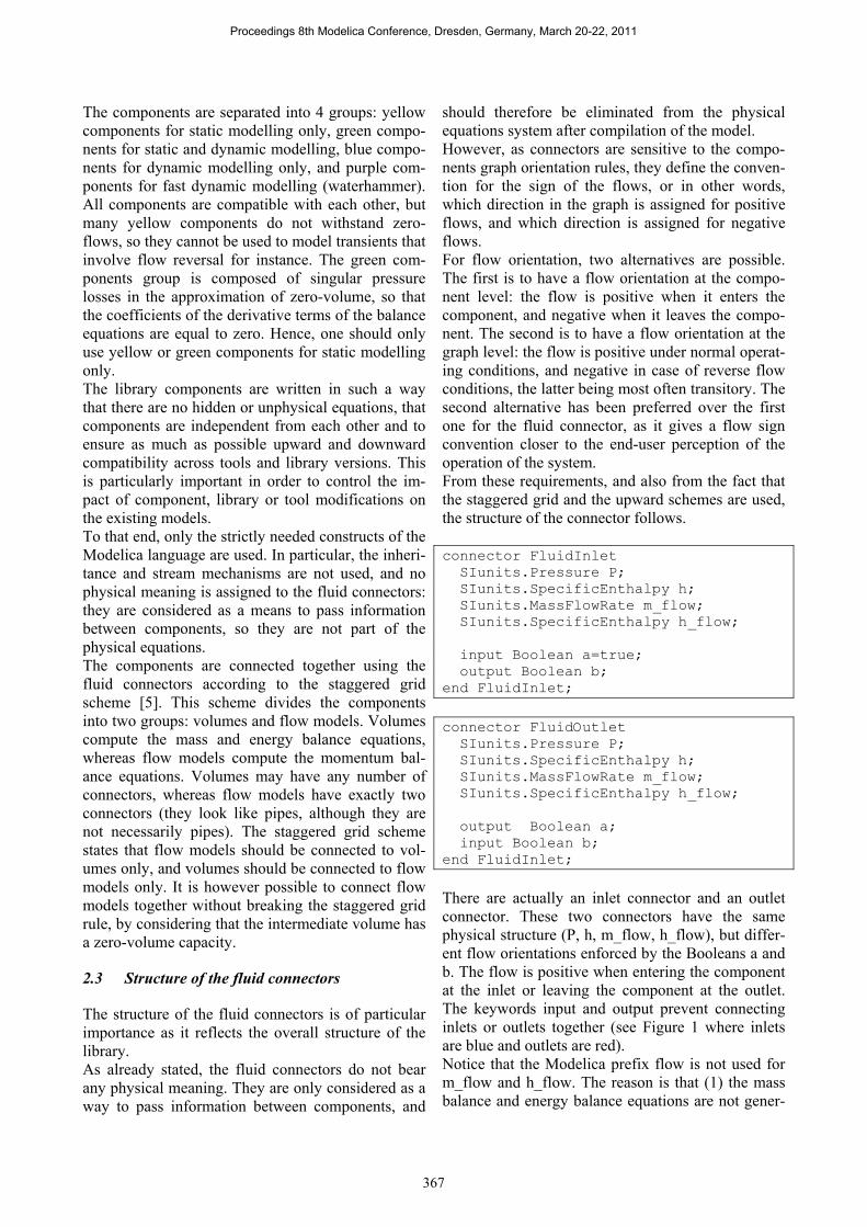
connector FluidInlet SIunits.Pressure P; SIunits.SpecificEnthalpy h; SIunits.MassFlowRate m_flow; SIunits.SpecificEnthalpy h_flow; input Boolean a=true; output Boolean b; end FluidInlet; connector FluidOutlet SIunits.Pressure P; SIunits.SpecificEnthalpy h; SIunits.MassFlowRate m_flow; SIunits.SpecificEnthalpy h_flow; output Boolean a; input Boolean b; end FluidInlet; There are actually an inlet connector and an outlet connector. These two connectors have the same physical structure (P, h, m_flow, h_flow), but differ-ent flow orientations enforced by the Booleans a and b. The flow is positive when entering the component at the inlet or leaving the component at the outlet. The keywords input and output prevent connecting inlets or outlets together (see Figure 1 where inlets are blue and outlets are red). Notice that the Modelica prefix flow is not used for m_flow and h_flow. The reason is that (1) the mass balance and energy balance equations are not gener-


367

ated by the connections, but fully implemented in the volumes, (2) and that the sign convention for posi-tive flows is not compatible with the sign convention of the Modelica flow prefix, which stipulates that all flows should be of the same sign (positive or nega-tive) when entering the component via the connector. As a consequence, multiple connections are not al-lowed as in Modelica.Fluid for instance, so that mergers or splitters must be modeled using volumes. In practice, this is not considered as a restriction, as in most cases, mergers or splitters do have non trivial physical behaviours which could not be simply rep-resented by multiple connections.

Figure 1: connecting components

P and h denote resp. the average fluid pressure and specific enthalpy inside the control volumes. m_flow and h_flow denote resp. the mass flow rate and spe-cific enthalpy crossing the boundary between two control volumes (see Figure 2).

P2, h2P1, h1m_flowh_flow

Control volume 1 Control volume 2

Figure 2: finite volume discretization

P, h and m_flow are the state variables of resp. the mass, energy and balance equations. h_flow is not a state variable. The purpose of h_flow is to compute the fluid specific enthalpy using the upwind scheme. P and h are computed within volumes, whereas m_flow and h_flow are computed within flow mod-els (see Figure 3).

P1, h1

Volume 1 Flow model Volume 2

21 )_()_(_ hflowmshflowmsflowh ⋅−+⋅=

)_,,(_ 21 flowhPPfflowm =P2, h2

Figure 3: staggered grid scheme

According to the upwind scheme: 21 )_()_(_ hflowmshflowmsflowh ⋅−+⋅=

where s denotes the step function: 0)( =xs if 0≤x and 1)( =xs if 0>x

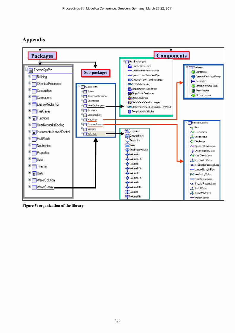
2.4 Organization of the library

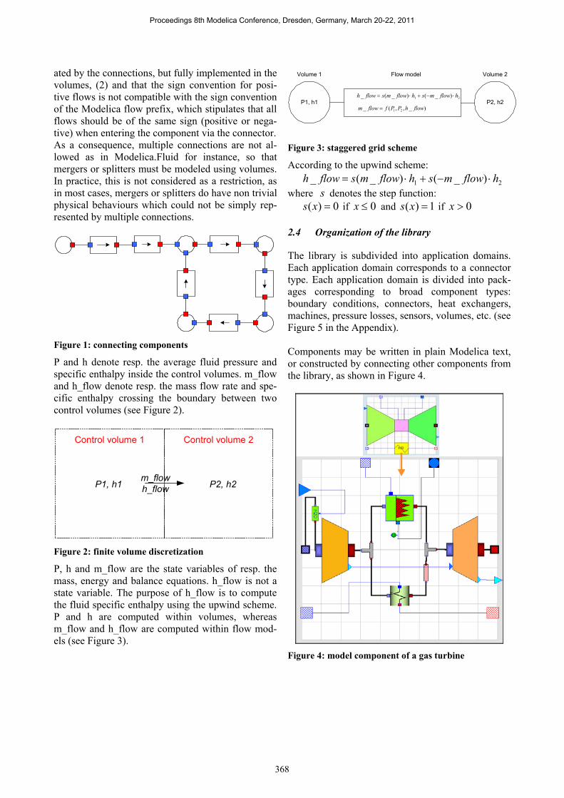
The library is subdivided into application domains. Each application domain corresponds to a connector type. Each application domain is divided into pack-ages corresponding to broad component types: boundary conditions, connectors, heat exchangers, machines, pressure losses, sensors, volumes, etc. (see Figure 5 in the Appendix). Components may be written in plain Modelica text, or constructed by connecting other components from the library, as shown in Figure 4.

Figure 4: model component of a gas turbine


368

3 Model of the combined cycle power plant

3.1 Description of the model

Actually, two models are used: one to simulate the power generator step reduction load (see Figure 6 in the Appendix), the other to simulate the full GT trip (see Figure 7 in the Appendix). In the model used to simulate the GT trip, the gas turbine is replaced by a boundary condition. The model contains two main parts: the water/steam cycle and the flue gases subsystem. Only one train is modelled, so identical behaviour is assumed for each HRSG and for each gas turbine.

HRSG model The model consists of 16 heat exchangers (3 evapo-rators, 6 economizers, 7 super-heaters), 3 evaporat-ing loops (low, intermediate and high pressure), 3 drums, 3 steam turbine stages (HP, IP and LP), 3 pumps, 9 valves, several pressure drops, several mixers, several collectors, 1 condenser, 1 generator, several sensors, sources, sinks and the control system limited to the drums level control. An important feature of this model is that the ther-modynamic cycle is completely closed through the condenser. This is something difficult to achieve, because of the difficulty of finding the numerical balance of large closed loops. The list of component used for the development of the HRSG model is given in Table 1. Table 1: library components used in the HRSG model

Type Model name in the library Condenser DynamicCondenser Drum DynamicDrum Generator generator Heat ex-changer

DynamicExchangerWaterSteamFlueGases = DynamicTwoPhaseFlowPipe ExchangerFlueGasesMetal HeatExchangerWall

Pipe LumpedStraightPipe Pump StaticCentrifugalPump Sensor SensorQ Steam tur-bine

StodolaTurbine

Valve ControlValve Water mixer VolumeB, VolumeC

Type Model name in the library Water split-ter

VolumeA, VolumeD

Heat Exchanger : Flue Gases/ Water Steam Based on first principles mass, momentum and en-ergy balance equations, the following phenomena are represented: - transverse heat transfer, - mass accumulation, - thermal inertia, - gravity, - pressure drop within local flow rate.

Drum and Condenser Based on first principles mass and energy balance equations for water and steam, the following phe-nomena are represented: - drum level and swell and shrink phenomenon, - heat exchange between the steam/water and the

wall, - heat exchange between the outside wall and the

external medium.

Steam turbine Based on an ellipse law and an isentropic efficiency.

Pump Based on the characteristics curves.

Pressure drop in pipes Proportional to the dynamic pressure ± the static pressure.

Mixer/splitter Based on the mass and energy balances for the fluid.

GT model The model consists of 1 compressor, 1 gas turbine, 1 combustion chamber, sources, sinks and 1 air humid-ity model. The list of component models used for the develop-ment of the GT model is given in Table 2.

Table 2: library components used in the GT model

Type Model name in the library Air humidity AirHumidity Compressor GTCompressor Gas turbine CombutionTurbine Combustion chamber

GTCombustionChamber

Gas turbine Based on correlations for the characteristic.


369

Compressor Based on correlations for the characteristic.

Combustion chamber Based on first principles mass, momentum and en-ergy balance equations. The pressure loss in the combustion chamber is taken into account.

3.2 Data implemented in the model

All geometrical data were provided to the model (pipes and exchangers lengths and diameters, heat transfer surfaces of exchangers, volumes…). The plant characteristics are given below.

Gas Turbine (GT) Compressor compression rate: 14

Steam Generator (HRSG) HRSG with 3 levels of pressure. High pressure circuit at nominal power: 128 bar Intermediate pressure circuit at nominal power: 27 bar Low pressure circuit at nominal power : 5.7 bar

Steam Turbine High pressure at nominal power : 124.5 bar, 815 K Intermediate pressure at nominal power : 25.5 bar, 801 K Low pressure at nominal power : 4.8 bar, 430 K

Condenser Steam flow rate: 194 kg/s Water temperature at the inlet: 300 K

3.3 Calibration of the model

The calibration phase consists in setting (blocking) the maximum number of thermodynamic variables to known measurement values (enthalpy, pressure) taken from on-site sensors for 100% load. This method ensures that all needed performance parame-ters, size characteristics and output data can be com-puted. The main computed performance parameters are: - the characteristics of the pumps, - the ellipse law coefficients of the turbines, - the isentropic efficiencies of the turbines, - the friction pressure loss coefficients of the heat

exchangers and of the pipeline between the equipments,

- the CV of the valves and the valves positions (openings).

3.4 Simulation scenarios

For simulation runs, two scenarios were selected. The first scenario is a power generator step reduction from 100 to 50% load: - Initial state (combined cycle): 100 % load - Final state (combined cycle): 50% load (800 s

slope) The second scenario is a full GT trip (sudden stop-ping of the gas turbine): - Initial state (GT exhaust): 894 K, 607 kg/s - Final state (GT exhaust): 423 K, 50 kg/s (600 s

slope) The following phenomena are simulated: - flow reversal, - local boiling or condensation, - swell and shrink effect in drums, - drums levels and condenser level, - drums pressure control

3.5 Simulation scenarios

Simulation runs were done using Dymola 6.1. The simulation of the scenarios were mostly success-ful. However, some difficulties were encountered when simulating large transients, mainly stemming from the large size of the model: - poor debugging facility, - slow simulation, - large number of values to be manually provided

by the user for the iteration variables, - no efficient handling of these values. In particular, it has been observed that sometimes Dymola cannot calculate the initial states, even when all iterations variables are set very close to their solu-tion values. This was the main difficulty that was encountered when closing the loop through the con-denser. When Dymola stops before the end of the simula-tion, no clear message is delivered to analyse the causes of the failure. Tool improvements were analysed and reported as part of the EDF contribution to the EUROSYSLIB project, in partnership with Politecnico di Mi-lano [6].

3.6 Simulation results

The model is able to compute precisely: - the air excess, - the distribution of water and steam mass flow

rates, - the thermal power of heat exchangers,


370

- the electrical power provided by the generator, - the pressure temperature and specific enthalpy

distribution across the network, - the drums levels and the condenser level, - the performance parameters of all the equip-

ments, - the global efficiencies of the water/steam cycle

and gas turbine. The computational time is faster than real time (with Dymola 6.1). The results of the simulation for 100% load are given below.

Gas Turbine (GT) Nominal power: 2*230 MW,

Steam Generator (HRSG) Thermal power: 2*350 MW,

Steam Turbine Nominal power: 275 MW,

Condenser Thermal power: 423 MW. Outlet water temperature: 306 K Vacuum pressure: 6100 Pa The results of the simulation runs are given in Figure 8 and Figure 9 in the Appendix. They are consistent with the engineer’s expertise. However, when the GT trip reaches full stopping of the plant, the recirculation flows in the evaporators do not go to zero as expected, for reasons that are not yet fully understood.

4 Conclusion

A new open source Modelica library called ‘Ther-moSysPro’ has been developed within the frame-work of the ITEA 2 EUROSYSLIB project. This library has been mainly designed for the static and dynamic modeling of power plants, but can also be used for other energy systems such as industrial processes, buildings, etc. It is intended to be easily understood and extendable by the models developer. Among other test-cases, a dynamic and rather large model of a combined cycle power plant has been developed to validate the library. This model com-prises the flue gas side and the full thermodynamic water/steam cycle closed through the condenser. Two difficult transients were simulated: a step reduc-tion load of the power generator and a full gas tur-bine trip. The results are mostly consistent with the engineer’s expertise.

Despite of some simulation difficulties because of the lack of debugging tools for Modelica models, this work shows that the library is complete and ro-bust enough for the modelling and simulation of complex power plants. However these two essential qualities for a power plant library should continu-ously be improved and maintained in the long run.

Acknowledgements

This work was partially supported by the pan-European ITEA2 program and the French govern-ment through the EUROSYSLIB project.

References

[1] Bouskela D., Chip V., El Hefni B., Faven-nec J.M., Midou M. and Ninet J. ‘New method to assess tube support plate clog-ging phenomena in steam generators of nuclear power plants’, Mathematical and Computer Modelling of Dynamical Sys-tems, 16: 3, 257-267, 2010.

[2] El Hefni B., Bouskela D., ‘Modelling of a water/steam cycle of the combined cycle power plant “Rio Bravo 2” with Mode-lica’, Modelica 2006 conference proceed-ings.

[3] Souyri A., Bouskela D., ‘Pressurized Wa-ter Reactor Modelling with Modelica’, Modelica 2006 conference proceedings.

[4] Collier J.G., and Thome J.R., ‘Convective Boiling and Condensation’, Mc Graw-Hill Book Company (UK) limited, 1972 Clar-endon Press, Oxford, 1996.

[5] Patankar S.V., ‘Numerical Heat Transfer and Fluid Flow’, Hemisphere Publishing Corporation, Taylor & Francis, 1980.

[6] Casella F., Bouskela D., ‘Efficient method for power plant modelling’, EDF report H-P1C-2010-01929-EN, 2010.

[7] David F., Souyri A., Marchais G., ‘Model-ling Steam Generators for Sodium Fast Reactors with Modelica’, Modelica 2009 conference proceedings

[8] El Hefni B., Péchiné B., ‘Model driven op-timization of biomass CHP plant design’, Mathmod conference 2009, Vienna, Aus-tria.


371

Appendix

PackagesPackages ComponentsComponents

Sub-packagesSub-packages

Figure 5: organization of the library


372

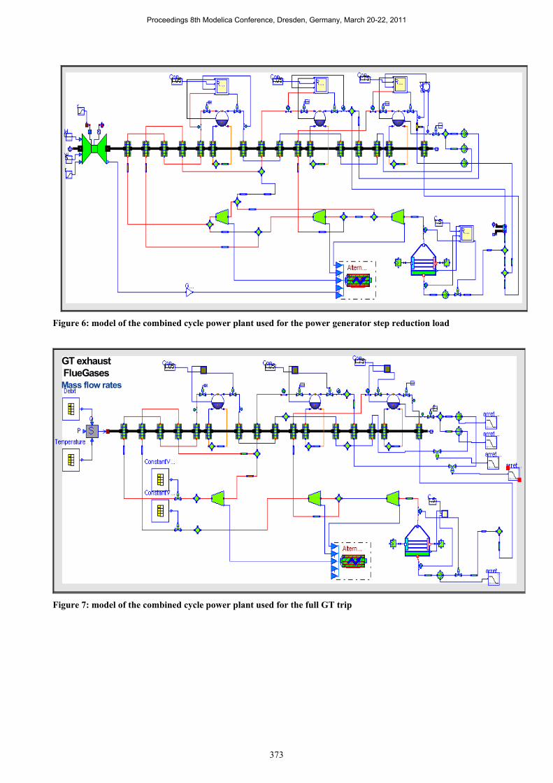
Figure 6: model of the combined cycle power plant used for the power generator step reduction load

Mass flow rates

GT exhaustFlueGases

Figure 7: model of the combined cycle power plant used for the full GT trip


373

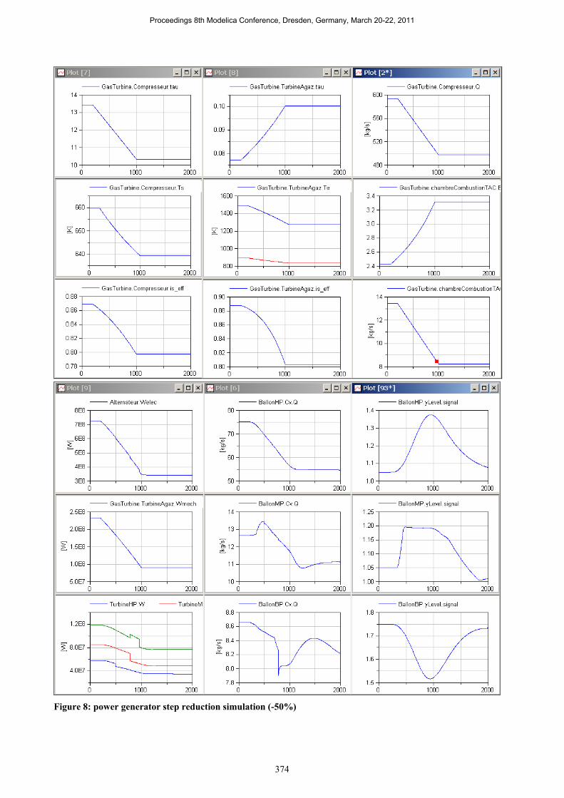
Figure 8: power generator step reduction simulation (-50%)


374

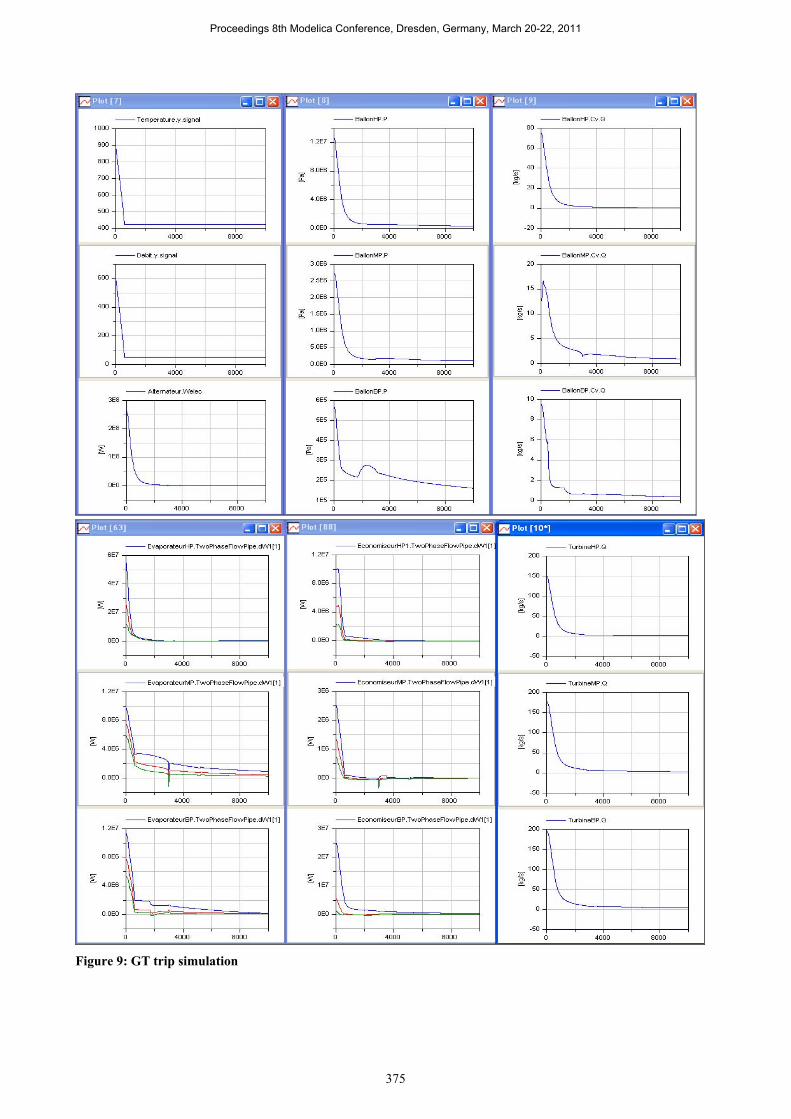
Figure 9: GT trip simulation


375

Documents

Dynamic modelling of a combined cycle power plant with ThermoSysPro · 2011-06-22 · Dynamic modelling of a combined cycle power plant with ThermoSysPro Baligh El Hefni Daniel Bouskela