Modelling of Combined Cycle Power Plant Ageing

in Matlab and IndustrialITr

A. Stothert, E. Gallestey and G.E. Hovland

Automation and Control Systems Group,ABB Corporate Research,

CH-5405 Baden-Dattwil, Switzerland,Fax: +41 56 486 7365

Abstract

This paper describes the development of a prototype deci-sion support product that indicates to a power plant operatorthe effect of daily operation on plant lifetime consumptionand recommends short-term operating strategies that opti-mise plant economic performance. The paper focuses on theuse of Matlab/ Simulink models, data structures, and userinterfaces used in this decision support tool. The complexityof the modelling requirements and sheer number of parame-ters resulted in extensive use of Matlab structures and cus-tom made Simulink libraries and proved to be the only viablemethod of creating a useable system. The final solution isintegrated with ABB’s IndustrialITrarchitecture.

1 Introduction

Power plant owners operating in deregulated energy marketsare under increasing pressure to improve their maintenancestrategies, minimise plant operating costs, and manage themarket value of their physical assets. A central componentin achieving these requirements is the accurate calculation ofproduction costs — plant depreciation and degradation re-sulting from production must be included in this calculation.In order to support power plant owners in this competitivederegulated environment a tool recommending plant oper-ating strategies has been developed. Recommending suchpower plant operating strategies is based on the optimisa-tion of an objective function that includes terms for revenuesfrom energy sales, production costs and plant ageing.

The developed tool focuses on combined cycle power plantswhich typically includes a gas turbine, heat recovery steamgenerator and steam turbine. The gas turbine exhaust gas isused to heat a water steam cycle and the resulting steam isused to drive a steam turbine. While topologies vary a typi-cal configuration is for the gas and steam turbine to share acommon rotor that is connected to an electrical generator.It is also often possible to operate the steam turbine in aby-pass mode, i.e., the generated steam is sold to processindustries or district heating rather than used for genera-tion of electricity. Combined cycle operating strategies arenormally chosen by forecasting future energy prices (bothelectricity and steam) and using ”cost of production curves”

to select the level of electricity and steam production [4, 5].In this article the cost of plant ageing is introduced intothe cost of production curves. In particular plant ageing isbased on models that are directly load dependent and in-corporate a memory aspect. This implies that optimisationresults in a trade-off between maximisation of immediateprofits (i.e., earnings achieved by selling heat and power)and minimisation of lifetime consumption.

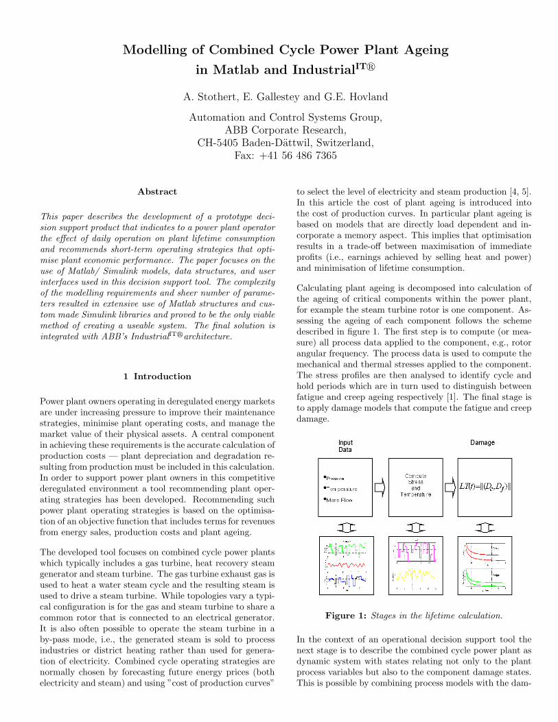
Calculating plant ageing is decomposed into calculation ofthe ageing of critical components within the power plant,for example the steam turbine rotor is one component. As-sessing the ageing of each component follows the schemedescribed in figure 1. The first step is to compute (or mea-sure) all process data applied to the component, e.g., rotorangular frequency. The process data is used to compute themechanical and thermal stresses applied to the component.The stress profiles are then analysed to identify cycle andhold periods which are in turn used to distinguish betweenfatigue and creep ageing respectively [1]. The final stage isto apply damage models that compute the fatigue and creepdamage.

Figure 1: Stages in the lifetime calculation.

In the context of an operational decision support tool thenext stage is to describe the combined cycle power plant asdynamic system with states relating not only to the plantprocess variables but also to the component damage states.This is possible by combining process models with the dam-

age models described above. The operational optimisationproblem can then be described in a model predictive con-trol framework [9] where the objective function is a weightedsum of the process and damage state variables.

The remainder of this paper is arranged as follows. Section 2describes the mathematics behind the process, ageing, andoptimisation models. Section 3 gives a detailed descriptionof the data structures, user interfaces and flow controls usedin the developed prototype product. Before concluding re-marks are given in section 5 section 4 briefly describes thestrategy for converting the prototype system into a finalproduct based on the ABB IndustrialITrplatform.

2 Mathematical Models

This section describes the models used in each of the stagesin figure 1. With the exception of the models used to spec-ify the model predictive control problem (see section 2.3)and the stress computations, which are modelled in mat-lab script files, all the models are implemented in simulink.Specifically both generic combined cycle power plant processmodels and damage models were implemented as simulinklibraries.

2.1 Process modelsSpace does not permit a detailed description of all the imple-mented process models. Note that generic models for, pipes,evaporators, heaters, separators, drums and economisers,attemporators, coolers and, turbine stages are sufficient fordamage modelling of key components in a combined cyclepower plant.

By way of a process example the model of a steam turbineconsists of inlet pipeing, a sequence of turbine stages andoutlet pipeing. Each stage in the steam turbine is modelledas follows [11]:

The rotor dynamics are described by a first order differen-tial equation relating angular acceleration to applied torques(Power produced minus demand and friction)

Idω

dt= P −D − cω2

The stages are divided into two sections, before and aftera vane. Each section is assumed polytropic and modelledas a pipe, the sections (and turbine stages) are connectedthrough mass balance equations, i.e., for stage i and thesection before the vane (subscript zero)

volidρi

dt= flowi

in − flowi

where

flow = ciρipi

√√√√1−(

pi0

pi1

)n+1n

flowiin = flowi−1

out

p0 = const(ρi0

)npolytropic flow

The power generated by each stage is an algebraic functionof the thermodynamic state of the stage and the stage ge-ometry.

2.2 Lifetime or damage modelsLifetime assessment of power plant components requires amultidisciplinary approach involving knowledge of design,material behaviour and non-destructive evaluation tech-niques. The literature available is vast and it is beyondthe scope of this paper to give a detailed account of thesemethods.

As indicated in the introduction two factors are critical forthe modelling of damage for optimisation purposes as re-quired here. Firstly the models have to provide a directrelationship between plant load and plant ageing, and sec-ondly the models must capture the operating history of thecomponent. Fracture mechanics provides a framework thatsatisfies these requirements, in particular the microcrackpropagation (MP) approach [2, 3], provides the requiredmodel features and gives a good theoretical basis for thecalculation of the lifetime of a component.

The main idea is as simple as it is appealing: a microcrackin a critical location or component is assumed to exist, andits propagation is modelled until a predefined critical cracksize is attained. The growth of the crack is modelled usingthe machinery developed in fracture mechanics.

While similar crack propagation under fatigue and creepconditions are described by different equations. The genericform is given by (1)

d a

dN=

C (max(Kmax −Kmin −Kth, 0))n

Kcrit/Kmax − 1(1)

whereK =

√πaσF (a/W )

Where a is the crack length, N the number of fatigue cy-cles, σ the applied stress, W , C, and n component specificconstants1, and F (a/W ) a function dependent on the ge-ometry of the component. K is the so called stress intensityfactor and the subscripts refer to the maximum and min-imum cycle stresses, the threshold stress below which nocrack growth occurs, and the critical stress which causesinstantaneous destruction of the component. Creep crackpropagation is described by an equation similar to (1) butdadN is replaced by da

dt .

In the simulink implementation F (a/W ) is implemented asa lookup table, (functions for different geometries are pub-lished in handbooks such as [8]) and the creep and fatigueequations are combined into one model. This is possible byusing a cycle identification algorithm for the fatigue equa-tion and the simulink reset integrator, see figure 2.

In order to convert the crack model into a cost that can beused in an optimisation problem a last step is required, viz.,the crack length is normalised according to a critical valueand component replacement cost, equation (2) illustrates

1C and n are material dependent and often vary with temperature.

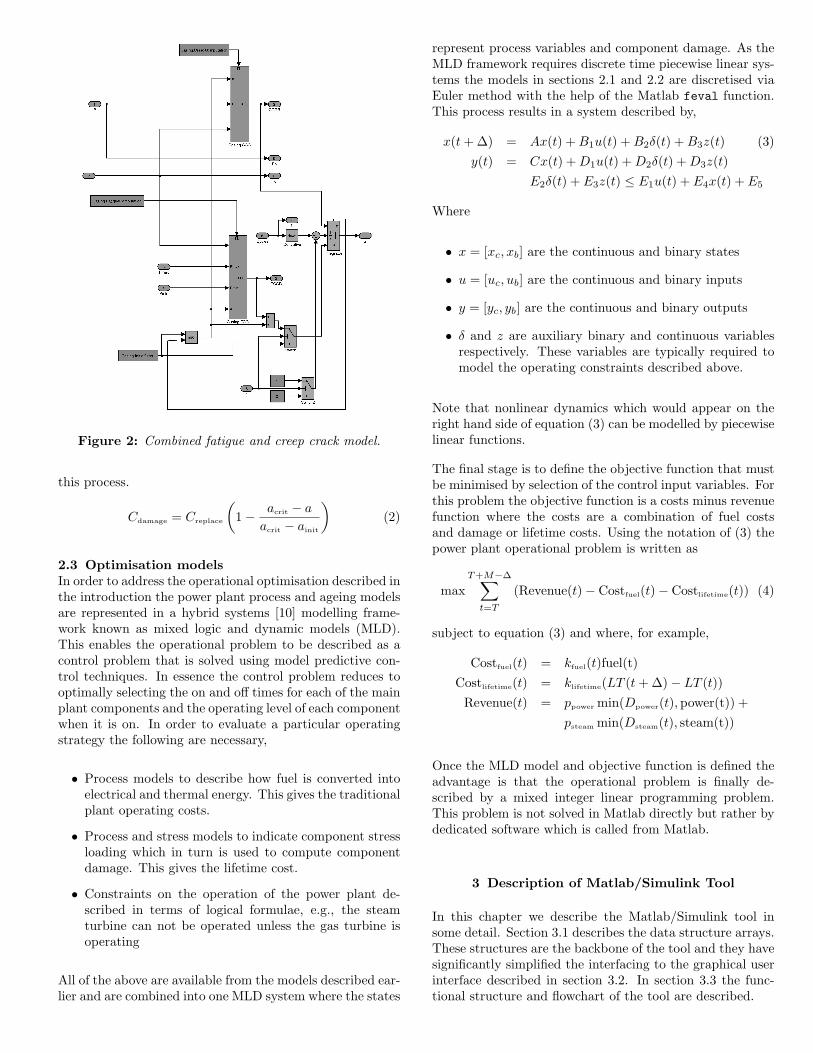
Figure 2: Combined fatigue and creep crack model.

this process.

Cdamage = Creplace

(1− acrit − a

acrit − ainit

)(2)

2.3 Optimisation modelsIn order to address the operational optimisation described inthe introduction the power plant process and ageing modelsare represented in a hybrid systems [10] modelling frame-work known as mixed logic and dynamic models (MLD).This enables the operational problem to be described as acontrol problem that is solved using model predictive con-trol techniques. In essence the control problem reduces tooptimally selecting the on and off times for each of the mainplant components and the operating level of each componentwhen it is on. In order to evaluate a particular operatingstrategy the following are necessary,

• Process models to describe how fuel is converted intoelectrical and thermal energy. This gives the traditionalplant operating costs.

• Process and stress models to indicate component stressloading which in turn is used to compute componentdamage. This gives the lifetime cost.

• Constraints on the operation of the power plant de-scribed in terms of logical formulae, e.g., the steamturbine can not be operated unless the gas turbine isoperating

All of the above are available from the models described ear-lier and are combined into one MLD system where the states

represent process variables and component damage. As theMLD framework requires discrete time piecewise linear sys-tems the models in sections 2.1 and 2.2 are discretised viaEuler method with the help of the Matlab feval function.This process results in a system described by,

x(t + ∆) = Ax(t) + B1u(t) + B2δ(t) + B3z(t) (3)y(t) = Cx(t) + D1u(t) + D2δ(t) + D3z(t)

E2δ(t) + E3z(t) ≤ E1u(t) + E4x(t) + E5

Where

• x = [xc, xb] are the continuous and binary states

• u = [uc, ub] are the continuous and binary inputs

• y = [yc, yb] are the continuous and binary outputs

• δ and z are auxiliary binary and continuous variablesrespectively. These variables are typically required tomodel the operating constraints described above.

Note that nonlinear dynamics which would appear on theright hand side of equation (3) can be modelled by piecewiselinear functions.

The final stage is to define the objective function that mustbe minimised by selection of the control input variables. Forthis problem the objective function is a costs minus revenuefunction where the costs are a combination of fuel costsand damage or lifetime costs. Using the notation of (3) thepower plant operational problem is written as

maxT+M−∆∑

t=T

(Revenue(t)− Costfuel(t)− Costlifetime(t)) (4)

subject to equation (3) and where, for example,

Costfuel(t) = kfuel(t)fuel(t)Costlifetime(t) = klifetime(LT (t + ∆)− LT (t))Revenue(t) = ppower min(Dpower(t),power(t)) +

psteam min(Dsteam(t), steam(t))

Once the MLD model and objective function is defined theadvantage is that the operational problem is finally de-scribed by a mixed integer linear programming problem.This problem is not solved in Matlab directly but rather bydedicated software which is called from Matlab.

3 Description of Matlab/Simulink Tool

In this chapter we describe the Matlab/Simulink tool insome detail. Section 3.1 describes the data structure arrays.These structures are the backbone of the tool and they havesignificantly simplified the interfacing to the graphical userinterface described in section 3.2. In section 3.3 the func-tional structure and flowchart of the tool are described.

Figure 3: Power plant component data structure.

3.1 Data StructuresThere is one main plant structure in the tool and for eachmajor aggregate i, such as a gas turbine, steam turbineor heat exchanger, there are three main data structures,Plant(i).Data, Plant(i).Comps and Plant(i).Results.The structure Plant(i).Comps is illustrated in Fig. 3. Thestructure Plant(i).data contains all configuration data forthe particular aggregate component. For example, the datastructure for a gas turbine contains values such as maximumload, number of turbine stages, nominal speed, etc. Thestructure Plant(i).Comps(j) contains the smallest com-ponents j of the plant. A gas turbine, for example, con-sists of a number of pipes, vanes and blades in addition tothe rotor and casing. Each of these smallest componentshas the data structure shown in Fig. 3. For each com-ponent j the Plant(i).Comp(j) structure contains geome-try and material parameters as well as process and ageingsimulations. Finally, the structure Plant(i).Results con-tains simulation and optimisation results directly relatedto the aggregate components, for example produced powerof the turbines, rotor speed, inlet flow, etc. All simula-tion and optimisation results which are not directly relatedto a component structure Plant(i).Comp(j) are stored inPlant(i).Results.

3.2 Graphical User InterfaceAn example of the graphical user interface (GUI) is shownin Fig. 4. The main feature of the GUI is the fact thatno hard-coding of presentation data is done. The only in-formation the GUI is given, is the global Plant structurewith the substructures Plant(i).Data, Plant(i).Compand Plant(i).Results as described in section 3.1. TheGUI loops through all aggregate components of the Plantstructure to display configuration data, process simulation,ageing simulations and optimisation results. By buildingthe GUI in this way, we have a very clear interface betweensimulation code and the GUI. Hence, a migration of thesimulation code to the ABB IndustrialITr architecture hasbeen significantly simplified. (For further comments aboutABB’s IndustrialITr architecture, see section 4.)

Moreover, when a completely new power plant is studied,the GUI remains unchanged. The addition of new aggre-gates, such as gas or steam turbines or a new topology ofthe heat exchanger (for example single-pressure drum in-

Figure 4: Graphical User Interface which loops through the datastructures and presents physical parameters, processand ageing simulations, and optimisation results.

stead of triple-pressure drums) is straightforward from theGUI point of view. For example, the Matlab code for dis-playing a list in the upper left part of Fig. 4 is given below.

set(Handles(LIndex),’Value’,CurrentAggregate);}set(Handles(LIndex),’String’,{Plant(:).type});}

The call Plant(:) loops through and displays all aggregatecomponents of the power plant.

3.3 Functional Structure and FlowchartThe functional structure is shown in Fig. 5. The toolconsists of a process simulation part, an ageing simula-tion part and an economic optimisation part. Fig. 6 il-lustrates the execution sequence from input to output data.Matlab/Simulink provides a powerful solution for modellingcombined cycle power plants of large complexity. The ex-ample presented here is taken from an operating combinedcycle power plant where over 400 equations (process mod-els, crack models, optimisaton functions, etc.) and over 3000parameters and results are used to describe the plant.

4 Integration with IndustrialITr

IndustrialITr (IIT) is an architecture for seamless linking ofmultiple applications and systems in real-time. This couldinclude e.g. process automation, asset optimisation and col-laborative business processes. It supports application reusefor higher quality and lower engineering costs, and simpleroperation, maintenance and training. It includes functional-ity ranging from field devices to business systems, focused onsupporting decisions and improving customer productivityand asset utilization, from the first phases of design, throughinstallation, commissioning, operation, maintenance and as-set optimization.

A key tool for migrating the Matlab/Simulink tool into anABB IIT product is the Aspect Integrator Platform (AIP).An sample screenshot from the AIP is shown in Fig. 7.

Figure 5: Overview of the functional structure of the complete tool. The tool consists of a process simulation part (aggregate.m andWholePlant.m), an ageing simulation part (Age.m, MaterialParameterEstimation.m and Stochastic.m) and an economicoptimisation part (MPC.m and LinMP MPC.m).

Central to the AIP is the Aspect Object Model which al-lows a user to present and manipulate information in acon-sistent way, features for easily integrating different functionsinto the AIP are also available. The Aspect Object Modelis based on the two ideas of Aspect Objects and Aspects.The objects in the model are the objects the user interactswith. For example, an object can be a turbine, a pipe or ablade. However, the object is simply a container that holdsdifferent parts, i.e., aspects of the object. An aspect is acollection of data and operations associated with an object.From a computer science perspective the Aspect Object is ameta-object that describes the aspects that, to a program-mer, are more normal OO objects. For more detailed infor-mation about the Aspect Object Model and the IntegratorPlatform, see [6, 7].

In the first phase of the product development, the datastructures, the simulation and optimisation routines in Mat-lab are kept, while the Matlab GUI is replaced by theIndustrialITr platform. Due to the clear interface betweenthe data structures and the GUI, it is relatively straight-forward to integrate the Aspect Objects with the Mat-lab/Simulink code.

The Aspect Integrator Platform provides the possibility oflinking to Matlab through an activeX connection and lettingMatlab run as a server on the platform. The MATLAB Run-

time Server provides one method for pushing variables to thematlab workspace: PutFullMatrix. Similarly, the outputfrom .m and .mdl files should be pushed on the Workspace,from which the aspect system object (GetFullMatrix) canread them. The combined Matlab/Simulink and Aspect In-tegrator Platform approach allows a fast transition fromprototype design to a customer product. However, the finalproduct release will port critical Matlab/Simulink modelsto compiled C++ code for speed improvements and intel-lectual property protection.

5 Conclusion

Estimating the true costs associated with operating a powerplant requires that the cost of damage resulting from operat-ing the plant be monitored and predicted. Once these costsare quantified a tool to support operation is possible. Thispaper has described how Matlab has been used to developsuch a prototype product.

The flexibility and ease of use of the Matlab/ Simulinkcombination meant that complex models and computationrequirements could be developed quickly. The paper con-cludes by briefly showing how the developed prototype sys-tem can be transferred to a commercial product based on

Figure 6: Flowchart of the complete tool. The diagram shows the execution sequence from input data to the final output data, optimalpower output trajectory. The optimal power output is computed for all gas and steam turbines. The cylinders illustratemodels, the squares illustrate algorithms and the parallelograms illustrate constant data and lookup tables.

Figure 7: Migration of Matlab data structure to ABB’s AspectIntegrator Platform.

ABB’s new IndustrialITrsolution architecture.

References

[1] R. Viswanathan, ”Damage Mechanisms and Life As-sessment of High-Temperature Components”, ASM Inter-national, 1989.

[2] M.P.Miller, D.C.McDowell, et.al, ”A life predictionmodel for thermomechanical fatigue based on microcrackpropagation”, ASTM STP 1186, 1993, pp 35-49.

[3] C.Cangan, et.al, ”Recent developments in the ther-momechanical fatigue lifetime prediction of superalloys”, e-JOM, Vol. 51. No 4. April 1999.

[4] R. Green, ”Competition in Generation: The Eco-nomic Foundations”, Proceedings of the IEEE, vol. 88, no.2, pp 128-139, February 2000.

[5] C. Wang, and S. Shahidehpour, ”Optimal GenerationScheduling with Ramping Costs”, IEEE Trans. on PowerSystems, Vol. 10, no. 1, pp 60-67. February 1995.

[6] ABB Automation Products, IndustrialITr: AspectObject Architecture Document, ABB Document Number3BSE 012 770R101, 2001.

[7] ABB Automation Products, IndustrialITr: AspectIntegrator Platform, Programmers Guide, ABB DocumentNumber 3BSE 023 959R101, 2001.

[8] D. Rooke and D. Cartwright, ”Compendium of StressIntensity Factors”, Her Majesty’s Stationery Office, 1976.

[9] E. Camacho and C. Bordons, ”Model Predictive Con-trol”, Springer 1999.

[10] A. Bemporad and M. Morari, ”Control of systems in-tegrating logic, dynamics, and constraints”, Automatica,Vol. 35, no. 3, pp 407–427, 1999.

[11] W. Traupel, ”Termische Turbomaschinen”, SpringerVerlag 1988.