Embed Size (px)
Citation preview
1 Copyright © 2008 by ASME
Proceedings of the 2008 International Design Engineering Technical Conference & Computers and Information and Information in Engineering Conference
IDETC/CIE 2008 August 3-6, 2008, New York City, NY, USA
DRAFT DETC2008-49062
DYNAMIC OBSERVER METHOD BASED ON MODIFIED GREEN’S FUNCTIONS FOR ROBUST AND MORE STABLE INVERSE
ALGORITHMS
Priscila F. B. Sousa Federal University of Uberlândia-School of Mechanical
Engineering, Brazil
Ana P. Fernandes Federal University of Uberlândia-School of Mechanical
Engineering, Brazil
Valério Luis Borges Federal University of Uberlândia-School of Mechanical
Engineering
George S. Dulikravich Florida International University- Department of
Mechanical and Materials Eng., Miami, FL, USA
Gilmar Guimarães Federal University of Uberlândia-School of Mechanical Engineering, Brazil
ABSTRACT
This work presents a modified procedure to use the concept of
dynamic observers based on Green’s functions to solve inverse
problems. The original method can be divided in two distinct
steps: i) obtaining a transfer function model GH and; ii)
obtaining heat transfer functions GQ and GN and building an
identification algorithm. The transfer function model, GH, is
obtained from the equivalent dynamic systems theory using
Green’s functions. The modification presented here proposes
two different improvements in the original technique: i) A
different method of obtaining the transfer function model, GH,
using analytical functions instead of numerical procedures, and
ii) Definition of a new concept of GH to allow the use of more
than one response temperature. Obtaining the heat transfer
functions represents an important role in the observer method
and is crucial to allow the technique to be directly applied to
two or three-dimensional heat conduction problems. The idea
of defining the new GH function is to improve the robustness
and stability of the algorithm. A new dynamic equivalent
system for the thermal model is then defined in order to allow
the use of two or more temperature measurements. Heat
transfer function, GH can be obtained numerically or
analytically using Green’s function method. The great
advantage of deriving GH analytically is to simplify the
procedure and minimize the estimative errors.
INTRODUCTION The inverse problem can be found in a large area of science
and engineering and can be applied in different ways. The great
advantage of this technique is the ability of obtaining the
solution of a physical problem that can not be solved directly.
Different techniques can be found in literature in the
solution of inverse heat conduction problem (IHCP). For
instance, the mollification method [1], the conjugate gradient
technique [2], the sequential function specification [3] or the
use of optimization techniques such as genetic algorithms [4],
simulated annealing [5] or golden section method [6].
Technique based on filter such as the Kalmn filter [7] or
dynamic observers [8,9] have also been employed for the
solution of the IHCP.
In the dynamic observer technique, the IHCP solution
algorithms are interpreted as filters passing low-frequency
components of the true boundary heat flux signal while
rejecting high-frequency components in order to avoid
excessive amplification of measurement noise [8]. The dynamic
observers technique proposed by Blum and Marquardt [8],
focused on the one-dimensional linear case, was extended to
solve an inverse multidimensional heat conduction problem by
Sousa et al. [9].
In order to deal with multidimensional thermal models,
Sousa proposed an alternative way of obtaining the heat
transfer function, GH, by using the Green function concept
instead of taking the Laplace transform of the spatially
discretized system. This procedure allows flexibility and
efficiency to solve multidimensional inverse problems.
Despite the flexibility and efficiency of this procedure the
way proposed in ref. [9] is complex and requires some ability to
obtain the heat transfer function. In order to simplify the
procedure, minimize the noise effect in GH, and give more
robustness and stability to the inverse algorithms some
modifications are proposed here.
2 Copyright © 2008 by ASME
This work proposes two different improvements in the
original technique: i) A different method of obtaining the
transfer function model, GH, using analytical functions instead
of numerical procedure, and ii) Definition of a new concept of
GH to allow the use of more than one temperature response.
NOMENCLATURE
a, b, c, L plate dimensions, m
k thermal conductivity, W/m2 K
q heat flux input, W/m2
T temperature, oC
t time, s
T0 initial temperature
x, y, z Cartesian coordinates, m
Y measured temperature, oC
f frequency, Hz
G Green’s function, m2K/W
GH heat conductor transfer function,
m2K/W
GQ signal transfer function, m2K/W
GN noise transfer function, m2K/W
s Laplace transform variable
X(t) input signal in time domain, W/m2
Y(t) output signal in time domain, oC
X(f) input signal in frequency domain, W/m2
Greek Symbols
α thermal diffusivity, m2/s
ρ density, kg/m3
θ temperature difference, oC
Subscripts
M relative to experimental data
i relative to integer variables
FUNDAMENTALS
The inverse problem solution based on dynamic observers
can be divided in two distinct steps: i) the obtaining of the
transfer function model GH; ii) the obtaining of the heat transfer
functions GQ and GN and the building algorithm identification.
A complete description of this technique can be found in the
work of Blum and Marquardt [8] and Sousa et al. [9].
This section presents a new procedure based on analytical
Green function concept to obtain the transfer function model.
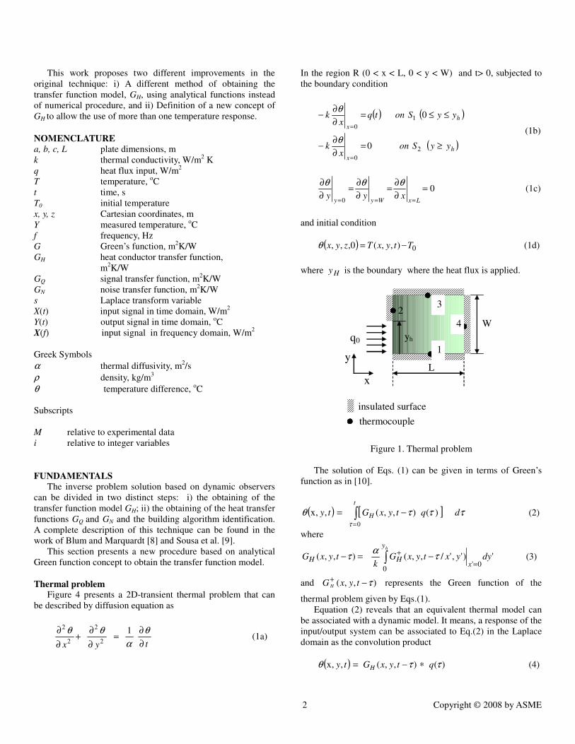
Thermal problem Figure 4 presents a 2D-transient thermal problem that can
be described by diffusion equation as
tyx ∂
∂=
∂
∂+
∂
∂ θ
α
θθ 12
2
2
2
(1a)
In the region R (0 < x < L, 0 < y < W) and t> 0, subjected to
the boundary condition
( ) ( )
( )h
x
h
x
yySonx
k
yySontqx
k
≥=∂
∂−
≤≤=∂
∂−
=
=
2
0
1
0
0
0
θ
θ
(1b)
0
0
=∂
∂=
∂
∂=
∂
∂
=== LxWyyxyy
θθθ (1c)
and initial condition
( ) 0),,(0,,, TtyxTzyx −=θ (1d)
where Hy is the boundary where the heat flux is applied.
W
y
L
q0
x
yh
insulated surface
thermocouple
1
2 3
4
Figure 1. Thermal problem
The solution of Eqs. (1) can be given in terms of Green’s
function as in [10].
( ) [ ] τττθτ
dqtyxGty
t
H∫=
−=0
)(),,(,,x (2)
where
∫=
+ −=−hy
xHH dyyxtyxG
ktyxG
00'
')','/,,(),,( τα
τ (3)
and ),,( τ−+ tyxG H represents the Green function of the
thermal problem given by Eqs.(1).
Equation (2) reveals that an equivalent thermal model can
be associated with a dynamic model. It means, a response of the
input/output system can be associated to Eq.(2) in the Laplace
domain as the convolution product
( ) )(),,(,,x ττθ qtyxGty H ∗−= (4)
3 Copyright © 2008 by ASME
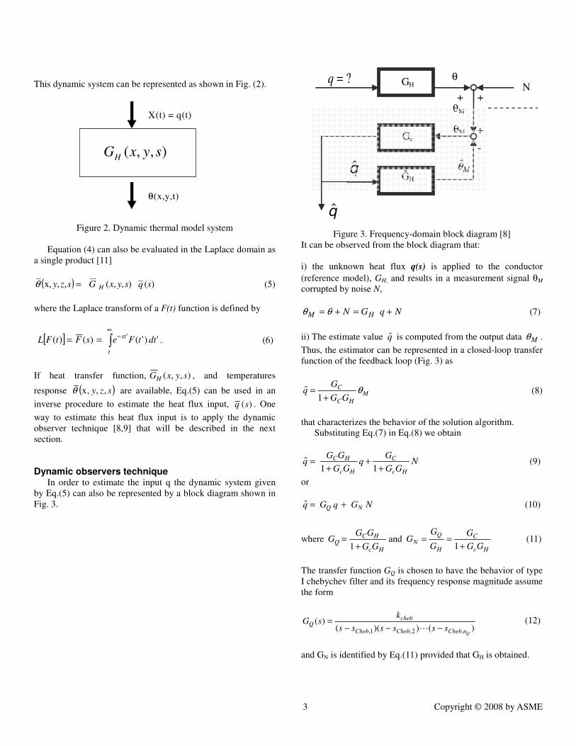
This dynamic system can be represented as shown in Fig. (2).
X(t) = q(t)
θ(x,y,t)
),,( syxGH
Figure 2. Dynamic thermal model system
Equation (4) can also be evaluated in the Laplace domain as
a single product [11]
( ) )(),,(,,,x sqsyxGszy H=θ (5)
where the Laplace transform of a F(t) function is defined by
[ ] ∫∞
−==t
stdttFesFtFL ')'()()(
'. (6)
If heat transfer function, ),,( syxGH , and temperatures
response ( )szy ,,,xθ are available, Eq.(5) can be used in an
inverse procedure to estimate the heat flux input, )(sq . One
way to estimate this heat flux input is to apply the dynamic
observer technique [8,9] that will be described in the next
section.
Dynamic observers technique In order to estimate the input q the dynamic system given
by Eq.(5) can also be represented by a block diagram shown in
Fig. 3.
GH N
Gc
ĜH
+
+ +
q
q
Mθ
θM
θM
-
?=q θ
Figure 3. Frequency-domain block diagram [8]
It can be observed from the block diagram that:
i) the unknown heat flux q(s) is applied to the conductor
(reference model), GH, and results in a measurement signal θM
corrupted by noise N,
NqGN HM +=+= θθ (7)
ii) The estimate value q is computed from the output data Mθ .
Thus, the estimator can be represented in a closed-loop transfer
function of the feedback loop (Fig. 3) as
M
HC
C
GG
Gq θ
+=
1ˆ (8)
that characterizes the behavior of the solution algorithm.
Substituting Eq.(7) in Eq.(8) we obtain
NGG
Gq
GG
GGq
Hc
C
Hc
HC
++
+=
11ˆ (9)
or
NGqGq NQ +=ˆ (10)
where Hc
HCQ
GG
GGG
+=
1and
Hc
C
H
Q
NGG
G
G
GG
+==
1 (11)
The transfer function GQ is chosen to have the behavior of type
I chebychev filter and its frequency response magnitude assume
the form
)())(()(
,2,1, QnChebChebCheb
chebQ
ssssss
ksG
−−−=
L (12)
and GN is identified by Eq.(11) provided that GH is obtained.
4 Copyright © 2008 by ASME
Thus, from Eq. (8) the resulting algorithm can then be given by
( ) ( ) ( )ssGsq MN θ×=ˆ (13)
or in domain frequency
( ) ( ) ( )jwjwGjwq MN θ×=ˆ (14)
It can be observed in Eq. (10) that if the algorithm estimates
the heat flux correctly, GQ is equal to unity, GQ = 1, and the
frequency w is within the pass band. In this case, the noise
transfer function GN is equal to the inverse transfer function of
the heat conductor (GH-1
).
According to Blum and Marquardt [8] the observer is
essentially an on-line scheme. In this case, estimation of the
heat flux at the current time step is based on current and past
temperature measurements only. In this case, any on-line
estimator involves a phase shift or lag. To remove this lag Blum
and Marquardt proposed a filtering procedure that can be
resumed in the use of two discrete-time difference equations
)()()(10
ikqaikYbkqnn n
i
iM
n
i
i −−−= ∑∑==
(15)
and
)(ˆ)()(ˆ10
ikqaikqbkqnn n
i
i
n
i
i −−−= ∑∑==
(16)
The coefficients ai and bi that appear in Eqs.(15) and (16) are
obtained using Eq.(11). In this case, the inverse procedure is
concluded with the ),,( syxGH identification.
Previous work presented by Sousa et al. [9] proposes the
identification of ),,( syxGH based on the cross correlation of
two functions of stationary random and in polynomial function
adjust of a particular sampled interval. Although efficient, the
technique requires some user’s ability that adds some
complexity to the optimization procedure.
The new procedure proposed here is to obtain the heat
transfer ),,( syxGH in an exact and analytical way.
Analytical heat transfer function identification, GH. If the dynamic system is linear, invariant and physically
invariable [11] the response function ),,,( szyxGH is the
same, independently of the pairs input/output. In this case, the
heat transfer function ),,,( szyxGH can, then, be obtained
through the auxiliary problem that is a homogenous version of
the original problem. The auxiliary problem is then solved for
the same region with a zero initial temperature and unit
impulsive source located at the region of the original heating
here represented by ( )szy ,,,x+θ .
It means ),,,( szyxGH can be obtained using Eq.(5) as
( )szysszyxGH ,,,x),,,(+= θ (17)
where s and ( )szy ,,,x+θ represent the Laplace transform of a
unit constant, s
L1
]1[ = , and a Laplace transform of the
temperature response of a unit step heat flux, ( )ty,,x+θ ,
respectively.
Temperature ( )ty,,x+θ can then be obtained by using
Green’s function method to solve the thermal problem
described by Eqs.(1) with heat flux input as
( )hyySonmWq ≤≤= 0/1 12 and ( )hyySonq ≥= 20
(18)
Thus, the solution of the problem given by Eqs.(1)
considering Eq.(18) is
( ) '),','/,,x(,,x
00'
'
dydtyxtyGk
ty
t
xxy
y
y
H
∫∫=
=
+ −+=τ
ττα
θ (19)
where
),'/,(),'/,x(),','/,,x( τττ ytyGxtGyxtyG yxxy = (20)
As the homogenous condition in both direction x and y are the
same, the Green functions can be given by
∑∞
=
−
+=1 1
)/'cos()/cos(1
m
mmtA
xN
LxLxe
LG
m ββ (21)
∑∞
=
−
+=1 2
)/'cos()/cos(1
m
nntA
yN
WxWye
WG
m γγ (22)
where πγπβ nmWNLN
nm ==== ,,21
,21
21
αβ
2
=
LA m
m and
2
=
WB
nn
γ
The substitution of Eqs.(20-22) into Eq.(19) gives
( )
++−
+
++=
∑ ∑∑ ∑
∑∑∑
∞
=
∞
=
−∞
=
−∞
=
−
∞
=
∞
=
∞
=
+
1 11 1
1111
,,x
n m
tFmn
m
tB
nn
tAm
nmn
mn
nm
nnm eAxyeAyeAx
tAAxyAyAxtyθ
(23)
where
5 Copyright © 2008 by ASME
( ) αγβ
+=+=
∗∗ 2
2
2
2 WLBAF nn
nnnand
nn
nnmmn
mm m
mm
nnn
nnn
F
WWW
N
Wy
N
Lx
kAxy
AN
LxWW
WkAx
BN
WWWWy
LkAy
WL
W
kA
1)/(sin)/cos()/cos(
1
)(
)/cos(1
1
)(
)/(sin)/cos(
1
1
1
21
1 1
21
2
1
11
∗
∗∗∗
∞
=∗
∗
∗∗
∗∗
=
=
+=
+=
∑
γ
γγβα
β
β
γγ
γγα
α
Taking the Laplace transform of Eq.(23) we obtain
( )
++
++
+−
+
+++=
∑∑∑∑
∑∑∑
∞
=
∞
=
∞
=
∞
=
∞
=
∞
=
∞
=
+
1 111
21111
0
111
11,,x
n m nmmn
nnn
m mm
nmn
nn
mm
FsAxy
BsAy
AsAx
sA
sAxyAyAxTsyθ
(2
4)
and therefore the heat transfer function in Laplace domains can
be obtained by substituting Eq.(24) in Eq.(17) to give
( )
++
++
+−+
+++==
∑∑∑∑
∑∑∑
∞
=
∞
=
∞
=
∞
=
∞
=
∞
=
∞
=
+
1 1111
1110
1
,,x),,(
n n nmmn
nnn
m nm
nmn
nm
mnH
Fs
sAxy
Bs
sAy
As
sAx
sA
AxyAyAxTsyssyxG θ
(25)
Since Eq.(25) does not present any pole for s>0 then its
inversion is stable. This fact guarantees more robustness to the
inverse algorithm.
Multiple sensors
Estimators given by Eq.(15) and (16) were derived to be
applied to single – input /output models. However, in order to
minimize the noise that appears in measurement data it may be
interesting to use more than one experimental measurement. In
this case the use of Green’s function method, with analytical or
numerical approach, also allow with simplicity to generalize the
use of that estimator. Following it will be formulated a dynamic
system with two output points due to a single source. The
extension for multiple points is very direct and immediate.
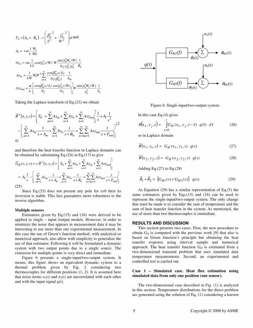
Figure 6 presents a single-input/two-output system. It
means, this figure shows an equivalent dynamic system to a
thermal problem given by Fig. 2 considering two
thermocouples for different positions (1, 2). It is assumed here
that noise terms n1(t) and n2(t) are uncorrelated with each other
and with the input signal q(t).
GH1(f)
GH2(f)
q(t)
θ1(t)
Y
∑
∑
n1(t)
n2(t)
θ2(t)
θM1(t)
θM2(t)
Figure 6. Single-input/two-output system.
In this case Eq.(4) gives
( ) ∫=
−=t
jHj dqtyGty
0
ii )(),,x(,,x
τ
τττθ (26)
or in Laplace domain
( ) )(),,x(,,x 1111 sqsyGsy H=θ (27)
( ) )(),,x(,,x 2222 sqsyGsy H=θ (28)
Adding Eq.(27) to Eq.(28)
[ ] )()()( 2121 sqsGsG HH +=+θθ (29)
As Equation (29) has a similar representation of Eq.(5) the
same estimators given by Eqs.(15) and (16) can be used to
represent the single-input/two-output system. The only change
that must be made is to consider the sum of temperature and the
sum of heat transfer function in the system. As mentioned, the
use of more than two thermocouples is immediate.
RESULTS AND DISCUSSION This section presents two cases. First, the new procedure to
obtain GH is compared with the previous work [9] that also is
based on Green function’s principle but obtaining the heat
transfer response using interval sample and numerical
approach. The heat transfer function GH is estimated from a
two-dimensional transient problem that uses simulated data
temperature measurements. Second, an experimental and
controlled test is carried out.
Case 1 – Simulated case. Heat flux estimation using
simulated data from only one position (one sensor).
The two-dimensional case described in Fig. (1) is analyzed
in this section. Temperature distributions for the direct problem
are generated using the solution of Eq. (1) considering a known
6 Copyright © 2008 by ASME
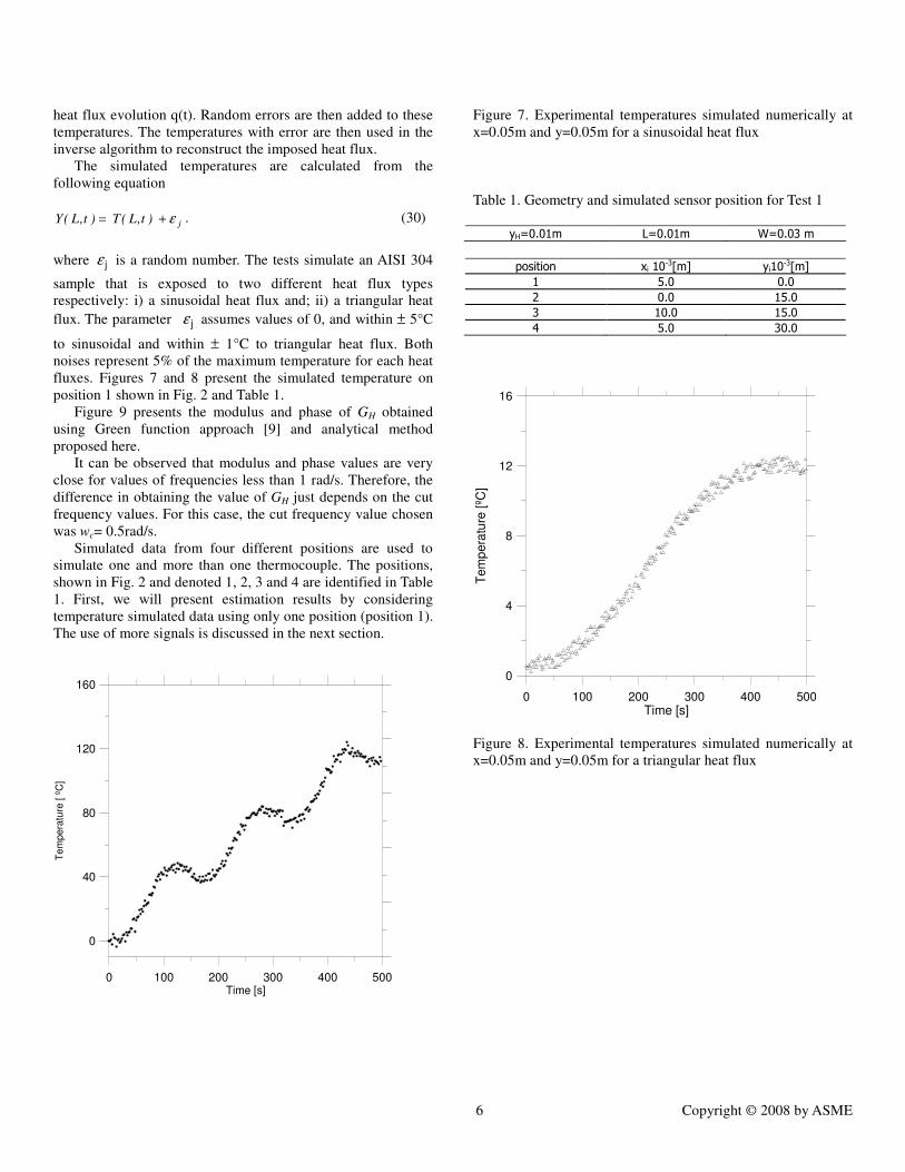
heat flux evolution q(t). Random errors are then added to these
temperatures. The temperatures with error are then used in the
inverse algorithm to reconstruct the imposed heat flux.
The simulated temperatures are calculated from the
following equation
j)t,L(T)t,L(Y ε+= . (30)
where jε is a random number. The tests simulate an AISI 304
sample that is exposed to two different heat flux types
respectively: i) a sinusoidal heat flux and; ii) a triangular heat
flux. The parameter jε assumes values of 0, and within ± 5°C
to sinusoidal and within ± 1°C to triangular heat flux. Both
noises represent 5% of the maximum temperature for each heat
fluxes. Figures 7 and 8 present the simulated temperature on
position 1 shown in Fig. 2 and Table 1.
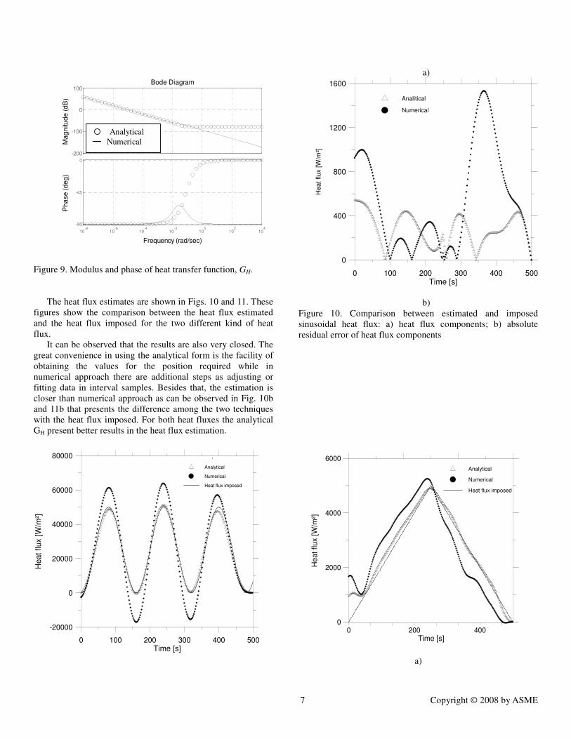
Figure 9 presents the modulus and phase of GH obtained
using Green function approach [9] and analytical method
proposed here.
It can be observed that modulus and phase values are very
close for values of frequencies less than 1 rad/s. Therefore, the
difference in obtaining the value of GH just depends on the cut
frequency values. For this case, the cut frequency value chosen
was wc= 0.5rad/s.
Simulated data from four different positions are used to
simulate one and more than one thermocouple. The positions,
shown in Fig. 2 and denoted 1, 2, 3 and 4 are identified in Table
1. First, we will present estimation results by considering
temperature simulated data using only one position (position 1).
The use of more signals is discussed in the next section.
0 100 200 300 400 500Time [s]
0
40
80
120
160
Te
mpera
ture
[ º
C]
Figure 7. Experimental temperatures simulated numerically at
x=0.05m and y=0.05m for a sinusoidal heat flux
Table 1. Geometry and simulated sensor position for Test 1
yH=0.01m L=0.01m W=0.03 m
position xi 10
-3[m] yi10-3[m]
1 5.0 0.0
2 0.0 15.0
3 10.0 15.0
4 5.0 30.0
0 100 200 300 400 500Time [s]
0
4
8
12
16
Tem
pera
ture
[ºC
]
Figure 8. Experimental temperatures simulated numerically at
x=0.05m and y=0.05m for a triangular heat flux
7 Copyright © 2008 by ASME
Bode Diagram
Frequency (rad/sec)
Ph
ase
(d
eg
)M
ag
nitu
de
(d
B)
-200
-100
0
100
Ghnum sensor 1
Ghana sensor 1
10-8
10-6
10-4
10-2
100
102
104
-90
-45
0
Analytical
Numerical
Figure 9. Modulus and phase of heat transfer function, GH.
The heat flux estimates are shown in Figs. 10 and 11. These
figures show the comparison between the heat flux estimated
and the heat flux imposed for the two different kind of heat
flux.
It can be observed that the results are also very closed. The
great convenience in using the analytical form is the facility of
obtaining the values for the position required while in
numerical approach there are additional steps as adjusting or
fitting data in interval samples. Besides that, the estimation is
closer than numerical approach as can be observed in Fig. 10b
and 11b that presents the difference among the two techniques
with the heat flux imposed. For both heat fluxes the analytical
GH present better results in the heat flux estimation.
0 100 200 300 400 500Time [s]
-20000
0
20000
40000
60000
80000
Heat flux [
W/m
²]
,
Analytical
Numerical
Heat flux imposed
a)
0 100 200 300 400 500Time [s]
0
400
800
1200
1600
Heat flux [W
/m²]
Analitical
Numerical
b)
Figure 10. Comparison between estimated and imposed
sinusoidal heat flux: a) heat flux components; b) absolute
residual error of heat flux components
0 200 400Time [s]
0
2000
4000
6000
He
at flu
x [
W/m
²]
Analytical
Numerical
Heat flux imposed
a)
8 Copyright © 2008 by ASME
0 100 200 300 400 500Time [s]
0
400
800
1200
1600
2000
He
at flux [
W/m
²]
Analytical
Numerical
b)
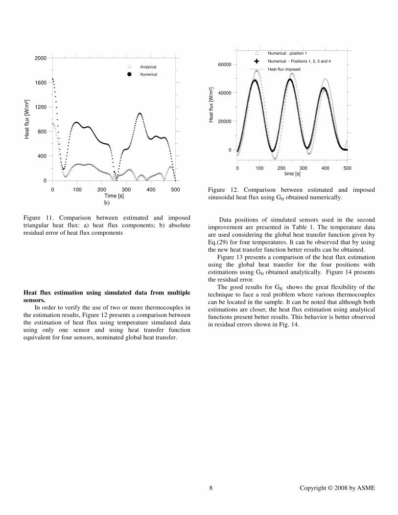
Figure 11. Comparison between estimated and imposed
triangular heat flux: a) heat flux components; b) absolute
residual error of heat flux components
Heat flux estimation using simulated data from multiple
sensors.
In order to verify the use of two or more thermocouples in
the estimation results, Figure 12 presents a comparison between
the estimation of heat flux using temperature simulated data
using only one sensor and using heat transfer function
equivalent for four sensors, nominated global heat transfer.
0 100 200 300 400 500time [s]
0
20000
40000
60000
Heat flux [W
/m²]
Numerical - position 1
Numerical - Positions 1, 2, 3 and 4
Heat flux imposed
Figure 12. Comparison between estimated and imposed
sinusoidal heat flux using GH obtained numerically.
Data positions of simulated sensors used in the second
improvement are presented in Table 1. The temperature data
are used considering the global heat transfer function given by
Eq.(29) for four temperatures. It can be observed that by using
the new heat transfer function better results can be obtained.
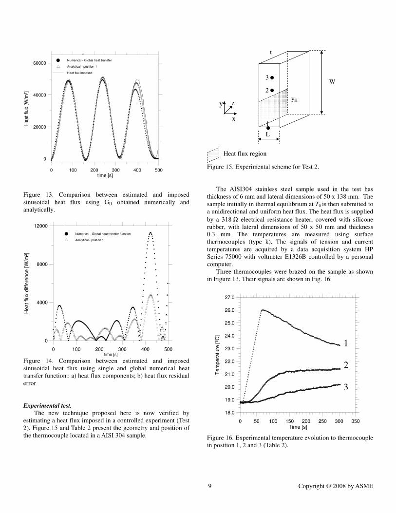
Figure 13 presents a comparison of the heat flux estimation
using the global heat transfer for the four positions with
estimations using GH obtained analytically. Figure 14 presents
the residual error.
The good results for GH shows the great flexibility of the
technique to face a real problem where various thermocouples
can be located in the sample. It can be noted that although both
estimations are closer, the heat flux estimation using analytical
functions present better results. This behavior is better observed
in residual errors shown in Fig. 14.
9 Copyright © 2008 by ASME
0 100 200 300 400 500time [s]
0
20000
40000
60000
He
at flu
x [W
/m²]
,
Numerical - Global heat transfer
Analytical - position 1
Heat flux imposed
Figure 13. Comparison between estimated and imposed
sinusoidal heat flux using GH obtained numerically and
analytically.
0 100 200 300 400 500time [s]
0
4000
8000
12000
Hea
t flu
x d
iffe
ren
ce
[W
/m²]
Numerical - Global heat transfer fucntion
Analytical - postion 1
Figure 14. Comparison between estimated and imposed
sinusoidal heat flux using single and global numerical heat
transfer function.: a) heat flux components; b) heat flux residual
error
Experimental test.
The new technique proposed here is now verified by
estimating a heat flux imposed in a controlled experiment (Test
2). Figure 15 and Table 2 present the geometry and position of
the thermocouple located in a AISI 304 sample.
yH
1
2
3
Heat flux region
y
x
W
L
t
z
Figure 15. Experimental scheme for Test 2.
The AISI304 stainless steel sample used in the test has
thickness of 6 mm and lateral dimensions of 50 x 138 mm. The
sample initially in thermal equilibrium at T0 is then submitted to
a unidirectional and uniform heat flux. The heat flux is supplied
by a 318 Ω electrical resistance heater, covered with silicone
rubber, with lateral dimensions of 50 x 50 mm and thickness
0.3 mm. The temperatures are measured using surface
thermocouples (type k). The signals of tension and current
temperatures are acquired by a data acquisition system HP
Series 75000 with voltmeter E1326B controlled by a personal
computer.
Three thermocouples were brazed on the sample as shown
in Figure 13. Their signals are shown in Fig. 16.
0 50 100 150 200 250 300 350Time [s]
18.0
19.0
20.0
21.0
22.0
23.0
24.0
25.0
26.0
27.0
Tem
pera
ture
[ºC
]
1
2
3
Figure 16. Experimental temperature evolution to thermocouple
in position 1, 2 and 3 (Table 2).
10 Copyright © 2008 by ASME
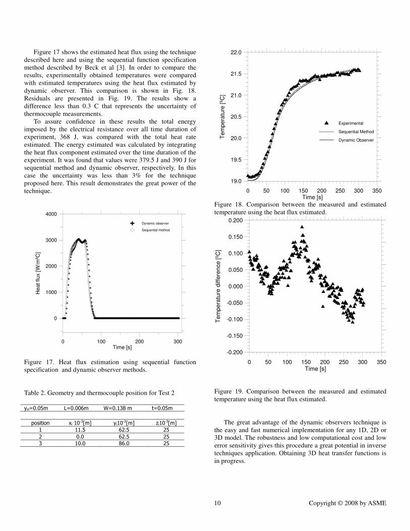
Figure 17 shows the estimated heat flux using the technique
described here and using the sequential function specification
method described by Beck et al [3]. In order to compare the
results, experimentally obtained temperatures were compared
with estimated temperatures using the heat flux estimated by
dynamic observer. This comparison is shown in Fig. 18.
Residuals are presented in Fig. 19. The results show a
difference less than 0.3 C that represents the uncertainty of
thermocouple measurements.
To assure confidence in these results the total energy
imposed by the electrical resistance over all time duration of
experiment, 368 J, was compared with the total heat rate
estimated. The energy estimated was calculated by integrating
the heat flux component estimated over the time duration of the
experiment. It was found that values were 379.5 J and 390 J for
sequential method and dynamic observer, respectively. In this
case the uncertainty was less than 3% for the technique
proposed here. This result demonstrates the great power of the
technique.
0 100 200 300Time [s]
0
1000
2000
3000
4000
He
at
flu
x [
W/m
ºC]
Dynamic observer
Sequential method
Figure 17. Heat flux estimation using sequential function
specification and dynamic observer methods.
Table 2. Geometry and thermocouple position for Test 2
yH=0.05m L=0.006m W=0.138 m t=0.05m
position xi 10
-3[m] yi10-3[m] zi10
-3[m]
1 11.5 62.5 25
2 0.0 62.5 25
3 10.0 86.0 25
0 50 100 150 200 250 300 350Time [s]
19.0
19.5
20.0
20.5
21.0
21.5
22.0
Tem
pera
ture
[ºC
]
Experimental
Sequential Method
Dynamic Observer
Figure 18. Comparison between the measured and estimated
temperature using the heat flux estimated.
0 50 100 150 200 250 300 350Time [s]
-0.200
-0.150
-0.100
-0.050
0.000
0.050
0.100
0.150
0.200T
em
pera
ture
diffe
rence [ºC
]
Figure 19. Comparison between the measured and estimated
temperature using the heat flux estimated.
The great advantage of the dynamic observers technique is
the easy and fast numerical implementation for any 1D, 2D or
3D model. The robustness and low computational cost and low
error sensitivity gives this procedure a great potential in inverse
techniques application. Obtaining 3D heat transfer functions is
in progress.
11 Copyright © 2008 by ASME
CONCLUSION
The dynamic observer technique based on analytical Green
function is presented here. The procedure used to obtain the
analytical heat transfer gives more flexibility and robustness to
the inverse procedure. The easiness of obtaining GH for any
position in the domain allows one to extend this technique to
use more than one measured temperature.
ACKNOWLEDGMENTS
The authors thank to CAPES, Fapemig and CNPq.
REFERENCES
1. D. A. Murio, The Molification Method and the
Numerical Solution of Ill-Posed Problems, John Wiley, New
York, 1993
2. O. M. Alifanov, Solution of na Inverse Problem of Heat
Conduction by Iterations Methods, Journal of Engineering
Physics, 10. (1975)
3. J. V. Beck, B. Blackwell, and C. R. St. Clair, Inverse
Heat Conduction, Ill-posed Problems, Wiley Interscience
Publication, New York, 1985
4. M. Raudensky, K. A. Woodbury, J. Kral, and T. Brezina,
Genetic Algorithm in Solution of Inverse Heat Conduction
Problems, Numerical Heat Transfer. Part B, 28, 293 (1995)
5. C. V. Gonçalves, L. O. Vilarinho, A. Scotti, and G.
Guimarães, G., Estimation of heat source and thermal efficiency
in GTAW process by using inverse techniques, Journal of
Materials Processing Technology,(2006)
6. S. R. Carvalho, S. M. M. Lima e Silva, A. Machado, G.
Guimarães, G., Temperature Determination at the Chip-tool
Interface Using an Inverse Thermal Model Considering the
Tool and Tool Holder, Journal of Materials Processing
Technology, (2006)
7. P. -C. Tuan, C-C. Ji, L.-W. Fong, and W.-T. Huang, An
Input Estimation Approach To On-Line Two-Dimensional
Inverse Heat Conduction Problems, Numerical Heat Transfer,
Part B, 29,345 (1996).
8 J.W. Blum and W. Marquardt, An optimal solution to
inverse heat conduction problems based on frequency-domain
interpretation and observers”, Numerical Heat Transfer, Part B:
Fundamentals, 32, 453 (1997).
9. Sousa, P. F. B., Development of a technique Based on
Green’s Functions and Dynamic Observers to be Applied in
Inverse Problems, , Dissertation of Master's degree, Federal
University of Uberlândia, Uberlândia, Mg. Brazil, 2006 (in
Portuguese)
10. J. V., Beck, K. D. Cole, A. Haji-Sheik, B. Litkouhi,,
Heat Conduction Using Green’s Function, Hemisphere
Publishing Corporation, USA, 1992, p. 523.
11. J. S. Bendat, A. G. Piersol, Analysis and Measurement
Procedures, Wiley-Intersience, 2nd
ed., USA, 1986, p. 566.