Dynamic Portfolio Allocation inGoals-Based Wealth Management ∗

Sanjiv R. Das∗

Santa Clara UniversityDaniel Ostrov

Santa Clara University

Anand RadhakrishnanFranklin Templeton Investments

Deep SrivastavFranklin Templeton Investments

May 23, 2019

Abstract

We report a dynamic programming algorithm which, given a set of efficient(or even inefficient) portfolios, constructs an optimal portfolio trading strategythat maximizes the probability of attaining an investor’s specified target wealthat the end of a designated time horizon. Our algorithm also accommodatesperiodic infusions or withdrawals of cash with no degradation to the dynamicportfolio’s performance or runtime. We explore the sensitivity of the terminalwealth distribution to restricting the segment of the efficient frontier availableto the investor. Since our algorithm’s optimal strategy can be on the efficientfrontier and is driven by an investor’s wealth and goals, it soundly beats theperformance of target date funds (TDFs) in attaining investors’ goals. Theseoptimal Goals-Based Wealth Management (GBWM) strategies are useful forindependent financial advisors (IFAs) to implement behavioral-based FinTechofferings and for robo-advisors.

Keywords: goals; wealth management; behavioral portfolio theory; dynamicportfolios; efficient portfolios.

∗We are grateful for discussions and contributions from many of the team at Franklin TempletonInvestments. Sanjiv Das (srdas@scu.edu, 408-554-2776, corresponding author) and Dan Ostrov(dostrov@scu.edu, 408-554-4551) are at 500 El Camino Real, Santa Clara, CA 95053. AnandRadhakrishnan (andy.radhakrishnan@franklintempleton.com, 800-632-2301) and Deep Srivastav(deepratna.srivastav@franklintempleton.com, 800-632-2301) are at 1 Franklin Pkwy #970, SanMateo, CA 94403.

1

1 Introduction

Goals-Based Wealth Management (GBWM) refers to the management of an investor’sportfolios with a view to meeting long-term financial goals, as opposed to only op-timizing a risk-return tradeoff. In this paper, we present and analyze a dynamicprogramming approach for GBWM that is fully optimal in meeting long-term goals,while also optimizing risk-return tradeoff. We will show that our approach has severaladvantageous features in terms of speed and adaptability, and that it soundly out-performs portfolios based on current widespread approaches, such as the target-dateparadigm.

GBWM is a modern implementation of behavioral ideas from early work by Shefrinand Statman (2000) espousing behavioral portfolio theory that were further discussedby Nevins (2004) from a practitioner viewpoint. A specific framework for GBWMwas initially proposed by Chabbra (2005) and is now followed by many practitioners(see Brunel (2015)). Our approach in this paper is also cognizant of prospect theory(Kahneman and Tversky (1979)), which is aimed at modeling how people realisti-cally make decisions, rather than an optimization framework, which usually does notaccount for all the criteria used by people when making tradeoffs between gains andlosses. Our framework also accommodates mental accounting (Thaler (1985); Thaler(1999)), which is the paradigm where people behave as if they have different risk-return preferences depending on the goal being achieved, being risk averse in somesettings and even risk seeking in others. In our context, mental accounting is the ideathat financial goals may be sharply defined and better managed in separate portfolios.We also include paradigms for how investors form both upside and downside goals,such as aspirational goal-setting (Lopes (1987)), a safety-first criterion (Roy (1952)),and loss aversion (Shefrin and Statman (1985)).

We can combine these seminal GBWM ideas for achieving long term goals withmodern portfolio theory (Markowitz (1952)) to achieve the short term goal of minimiz-ing the risk associated to any specific expected return. GBWM is fully consistent withMarkowitz’s mean-variance theory. This was developed in Das, Markowitz, Scheid,and Statman (2010) as a static model for mental accounts, while a full analysis of thestatic model in a GBWM context is provided in Das, Ostrov, Radhakrishnan, andSrivatav (2018).

These static models are not fully optimal, because they can only be implementedperiod by period in a myopic manner. Previous fully optimal, dynamic approachesto GBWM include solving continuous-time partial differential equations, as shownin the early work by Merton (1969); Merton (1971); Browne (1995); Browne (1997),or using continuous-time martingale methods based on seminal ideas in Cox andHuang (1989), as shown in more recent work by Wang, Suri, Laster, Almadi (2011)and Deguest, Martellini, Milhau, Suri, and Wang (2015). In this paper we intro-duce a discrete time fully optimal dynamic programming approach that has manyadvantages, including being adaptable to many financial situations, being simple toimplement, and being fast to run. For example, our approach handles periodic infu-

2

sions and withdrawals of varying amounts, as well as bankruptcy, which is not alwayseasy to do with the aforementioned continuous-time approaches. Also, our approachemploys a polynomial time algorithm that corresponds in general to a runtime of onlya few seconds. These features give our algorithm wide applicability, enabling eithertraditional financial advisors or robo-advisors to quickly and optimally determine thebest strategy for investors to pursue to meet their individual wealth goals.

The essence of GBWM lies in choosing a different objective function for dynamicoptimization than that chosen in utility-based portfolio problems. The simplest formof the GBWM objective function is probabilistic: that is, define a portfolio goal wealthG at the defined horizon T and find the dynamic portfolio strategy that maximizesthe probability of achieving the goal, i.e.,

max{A(0),A(1),...,A(T−1)}

Pr[W (T ) ≥ G],

whereW (T ) is the terminal portfolio wealth value andA(t) are the possible allocationsamong the funds available to the investor at each time t = 0, 1, 2, ..., T − 1. Theoptimal allocation at any time t is a function of W (t), the level of wealth at time t;G, the goal wealth; T , the timeframe; and other investor specific parameters.

This approach may be contrasted with a utility-based approach where the dynamicstrategy is chosen to maximize the expected utility from any consumption over time,as well as the expected utility of the final wealth. This approach, as well as GBWM,are attractive since they focus on long-run outcomes and are not myopic one-periodoptimization models. Single-period optimization changes the focus from achievinglong-term goals to short-term risk-return tradeoffs. We see that strategies that areaimed at meeting an upside goal with a lower threshold might result in very differentstrategies than dynamic asset allocation based on utility function maximization, suchas taking on more risk when not reaching goals close to the investment horizon, seeBrowne (1999b).

Hybrid approaches, where the objective function to be maximized is expected util-ity subject to goals as constraints, have also been attempted as in Browne (1999a);Browne (2000); Deguest, Martellini, Milhau, Suri, and Wang (2015). However, thisapproach requires choosing a utility function for the investor which is hard to de-termine, and therefore an ad-hoc choice is often required. In this paper, we do notrequire a utility function to be specified. We provide an optimal solution procedureto the GBWM problem and examine the properties of the trading strategy dictatedby the algorithm.

The following briefly characterizes our solution: (i) In our numerical experiments,the backward recursion algorithm that solves the dynamic problem is approximatelyquadratic in its dependence on the timeframe T , between linear and quadratic witha growth exponent of 1.5 in its dependence on the granularity of the wealth grid,and approximately linear in its dependence on the number of portfolio choices. Ourresults are quite robust to the granularity of the wealth grid and the number of port-folio choices, which suggests that expanding the scale of the problem with additional

3

features, such as tax optimization, can be performed without significantly degradingrun times or the solution’s accuracy. (ii) In our base case timeframe of ten yearswith annual rebalancing, having a wealth grid granularity of at least three wealthnodes per yearly standard deviation in portfolio performance, and allowing for 15portfolio choices, our algorithm runs in under five seconds. (iii) As the markets moveup or down through the investment tenure, we rebalance the portfolio such that theprobability of reaching the goal wealth continues to remain the highest. The optimalallocation and rebalancing is intuitive in the sense that when the portfolio is far fromits goal due to underperformance, risk is increased in order to enhance the proba-bility of reaching the goal, and when the portfolio is outperforming, risk is dialedback to reduce the risk of missing the goal. Therefore, the strategy depends on bothtime and state (wealth), unlike target-date fund strategies, which only depend ontime and cannot accommodate investor-specific goals. (iv) The dynamic programuses a collection of exogenously provided portfolios, that may or may not be cho-sen to be on the efficient frontier, so an asset management team can develop theset of model portfolios, while, acting separately, the optimization team can tune thedynamic programming algorithm. This offers a plug-and-play approach to GBWM,where portfolio construction is separated from portfolio allocation.

Our GBWM strategy allows for a variety of important features and results: (i)The final wealth distribution may be modulated by limiting the range of availableportfolios (i.e., controls), which exogenously alters the risk that is taken. Raising theminimum risk of the portfolios that are available to the investor increases the right tailof the wealth distribution more than the left tail. Conversely, raising the maximumrisk available to the investor, increases the left tail more than the right tail. Thissuggest that investors in a GBWM environment who wish to have higher returns arebetter off raising their minimum risk, instead of the more intuitive move of raisingtheir maximum risk. That said, raising the minimum risk will decrease the chanceof attaining the investor’s goal wealth, while raising the maximum risk will increasethis chance. (ii) The algorithm is flexible: (a) If desired, the algorithm can optimizefor multiple wealth goals at the end of the portfolio horizon instead of a single wealthgoal, with weights for the relative importance of these multiple goals that the investorcan decide. (b) The algorithm can include an investor’s specified portfolio infusionsand withdrawals. We will see that even small infusions can increase the probabilityof reaching the goal wealth substantively. When there are withdrawals, there is achance that the investor will run out money (i.e., go bankrupt) during the investmenttimeframe. Our algorithm can determine this chance of bankruptcy, and much moreimportantly, show how to minimize it. (c) The algorithm can accommodate any de-sired time period between rebalancing and between infusions or withdrawals. (iii)Our algorithm allows us to determine how to optimize retirement savings. For ex-ample, our algorithm will allow us to explore the effect of infusions on the minimizedprobability of going bankrupt in retirement. In particular, we will consider a 50 yearold investor who currently has 100 thousand dollars in their retirement account andintends to take out 50 thousand present day dollars every year after they turn 65through the age of 80. We show that to attain a 58.6% probability of maintaining

4

this income stream would require the investor to make annual inflation-adjusted infu-sions of 15 thousand dollars a year until retiring at age 65. (iv) Finally, we compareour GBWM optimal strategy to the performance of target date funds (TDFs), byconsidering a TDF with a typical glide path for three index funds representing to-tal domestic bond, total international stock, and total domestic stock. Because ourGBWM strategy is on the efficient frontier, uses a wealth dependent strategy, andaccounts for investor-specific goals, we will see that our GBWM strategy, which usesthe same three index funds, shows a much higher probability of reaching an investor’sgoals. For example, we will show that using our TDF in the case presented in theprevious point reduces the probability of maintaining the desired income stream from58.6% down to 26.6%.

The rest of this paper is organized as follows. In Section 2 we describe the algo-rithm and in Section 3 the extensions of the algorithm to deal with other cases arepresented. The results of our study are set out in Section 4 and our conclusions aresummarized in Section 5.

2 Algorithm

2.1 Notation

We describe the notation used in the paper here.

• Let t = 0, h, 2h, ..., Nh = T be the N time periods in the model. Here, h is thetime step, usually taken to be 1 year. Therefore, the time frame of the modelis 0 ≤ t ≤ T .

• Initial wealth: W (0).

• Target wealth (goal G) at the horizon: W (T ) ≡ G.

• We have n equity assets indexed by i = 1, 2, ..., n.

• C(t): known cash flows C(t) of capital into the portfolio each year. WhenC(t) > 0, we have an infusion into the portfolio. When C(t) < 0, we havea withdrawal from the portfolio. All of these cash flows are assumed to bedetermined at t = 0, so they are pre-committed by the investor.

Our goal is to dynamically allocate the portfolio among these n assets so that wemaximize the probability at t = T of attaining a final portfolio worth at least W (T ) =G, our goal wealth.

5

2.2 The Efficient Frontier for Stock Portfolios

For any given portfolio volatility, σ, it is always optimal to maximize the portfolioexpected return, µ. Modern portfolio theory, which was developed by Markowitz,see Markowitz (1952), gives a method for the exact allocation among the n assetsthat gives the maximum µ. If, for every value of σ, we plot the point (σ, µ) whereµ is the maximum portfolio expected return from modern portfolio theory, we sketchout a hyperbola in the (σ, µ) plane, which is called the efficient frontier. It is alwaysoptimal to maintain the portfolio on the efficient frontier. The question that remainsis how to optimally adjust ourselves along the efficient frontier over time.

As shown in Das, Ostrov, Radhakrishnan, and Srivatav (2018), the specific hy-perbola for the efficient frontier is the equation

σ =√aµ2 + bµ+ c. (1)

The constants, a, b, and c are defined by m, which is a vector of the n expectedreturns; o, which is a vector of n ones; and Σ, which is the n× n covariance matrixof the n assets, via the following equations:

a = h>Σh

b = 2g>Σh

c = g>Σg,

where the vectors g and h are defined by

g =lΣ−1o− kΣ−1m

lp− k2

h =pΣ−1m− kΣ−1o

lp− k2,

and the scalars k, l, and p are defined by

k = m>Σ−1o

l = m>Σ−1m

p = o>Σ−1o.

We allow for restrictions on the segment of the efficient frontier available to theinvestor, due, for example, to restrictions such as disallowing short positions. We willconsider this truncated efficient frontier as the set of potential portfolios from whichwe optimize the probability of attaining our goal wealthG. More specifically, we defineµmin and µmax to be the smallest and largest values of µ in this truncated efficientfrontier. The optimal policy or “control” in our problem is a value of µ ∈ [µmin, µmax],where the corresponding value of σ, the volatility, is given by equation (1).

Because it is optimal, we stay on the efficient frontier in this paper. However,we note that the method presented in this paper also applies to any fixed groupof allowable portfolios on or off the efficient frontier. So, for example, if there arelimitations on the fractions that can be devoted to specific assets within the portfolio,our method can still be applied.

6

2.3 The State Space Gridpoints

The state space consists of time values, t, and wealth values, W (t), which are dis-cretized, so that we consider annual rebalancing (and, later, non-annual rebalancingin Subsection 3.1) at times t = 0, 1, 2, . . . , T and, at each of these times, we usewealth grid points, Wi, where the index i ∈ {0, 1, 2, . . . , imax}. The smallest wealthgrid point, W0, should correspond to the smallest possible wealth, Wmin, attainable,and the largest wealth grid point, Wimax , should correspond to the largest possiblewealth, Wmax, attainable. We next determine values for imax,Wmin, and Wmax.

To move forward in time, we require a stochastic model for the evolution of theinitial portfolio wealth, W (0). We have chosen to use geometric Brownian motion forthis paper. That is,

W (t) = W (0)e

(µ−σ

2

2

)t+σ√tZ, (2)

where Z is a standard normal random variable, however, we could have just as easilyworked with other stochastic models, including those containing tails that are fatterthan normal distributions to more accurately reflect observed volatility. The onlyrestriction on the evolution model is that it is Markovian. That is, the evolutionmodel is not affected by previous events.

For our geometric Brownian motion model, we will assume that Z realisticallytakes values between −3 and 3, so the smallest realistic value for W (t) correspondsto computing equation (2) after setting Z = −3, µ = µmin, and σ equal to σmax,which is the value of σ from equation (1) when µ = µmax. The largest realistic valueis computed by again using σ = σmax, but replacing Z with 3 and µ with µmax.

Since we must also include the effects of the cashflows, C(t), as well as the initialinvestment, W (0), and both are affected by the same geometric Brownian motionmodel, we have that

Wmin = minτ∈{0,1,2,...,T}

[W (0)e

(µmin−

σ2max2

)τ−3σmax

√τ

+τ∑t=0

C(t)e

(µmin−

σ2max2

)(τ−t)−3σmax

√τ−t]

(3)

Wmax = maxτ∈{0,1,2,...,T}

[W (0)e

(µmax−

σ2max2

)τ+3σmax

√τ

+τ∑t=0

C(t)e

(µmax−

σ2max2

)(τ−t)+3σmax

√τ−t], (4)

where C(0) = 0, since any cash flow at t = 0 is incorporated into W (0). For themoment, we assume that Wmin > 0, because the C(t) are not sufficiently negativethat bankruptcy is a realistic possibility; in Section 3.2 we will explore the case whereC(t) are sufficiently negative that bankruptcy is a realistic possibility.

7

We next look to fill in the grid points between Wmin and Wmax. First, analogousto our σmax definition, we define σmin to be the value of σ from equation (1) whenµ = µmin. We then define the exogenously selected wealth grid density parameter,ρgrid, which corresponds to the number of wealth grid points chosen per each σmin inthe following sense: After setting t and Z to one in equation (2) and ignoring the drift

term(µ− σ2

2

)t, we see that σ is proportional to the logarithm of wealth. Therefore,

we compute ln(Wmin) and ln(Wmax) and then, starting with ln(Wmin), we add a gridpoint every σmin

ρgridunits, stopping once we reach or surpass ln(Wmax). This yields a

total of imax + 1 grid points where imax equals(ln(Wmax)−ln(Wmin))ρgrid

σminafter rounding up

to the nearest integer.

Next, we equally shift all of these imax + 1 values downward by the smallestamount necessary to match one of these values to ln(W (0)), the logarithm of theinitial portfolio wealth. Finally, we exponentiate all imax + 1 values to obtain ourwealth grid values, W0 through Wimax , noting the following: 1) One of the grid pointswill equal W (0), which will be important for computing the probability distributionfor the wealth in Subsection 2.5. 2) We define Wmin = W0 and Wmax = Wimax ,observing that the small downward shift will have created a small difference betweenWmin and Wmin and between Wmax and Wmax. 3) While the values of ln(Wi) wherei = 0, 1, 2, . . . , imax are equally spaced, the values of Wi are not. The spacing betweenWi values increases exponentially as the wealth increases.

2.4 Dynamic Programming for Optimizing the Chance ofObtaining the Investor’s Goal

The value function, V (W (t)), is the probability that the investor will attain their goalwealth, G, or more at the time horizon T , given they have a worth W (t) at time t.This means that at time T ,

V (Wi(T )) =

{0 if Wi(T ) < G1 if Wi(T ) ≥ G.

(5)

We next determine the Bellman equation so that we can determine V at yeart = T − 1, then t = T − 2, etc., iterating backwards in time until we finish att = 0. We begin by determining the transition probabilities, p(Wj(t + 1)|Wi(t), µ).The transition probability is the normalized relative probability that we will be atthe wealth node Wj at time t + 1 if we start at the wealth node Wi at time t and,between times t and t + 1, our portfolio is run with an expected return of µ and itscorresponding volatility, σ, from equation (1). Defining φ(z) to be the value of theprobability density function of the standard normal random variable at Z = z, wehave from equation (2) the following probability density function values

p(Wj(t+ 1)|Wi(t), µ) = φ

(1

σ

(ln

(Wj

Wi + C(t)

)−(µ− σ2

2

))). (6)

8

Normalizing these probability density function values yields the desired transitionprobabilities:

p(Wj(t+ 1)|Wi(t), µ) =p(Wj(t+ 1)|Wi(t), µ)

imax∑k=0

p(Wk(t+ 1)|Wi(t), µ)

.

Since V (W (t)) is the expected value of V (W (T )), our Bellman recursion equationis simply

V (Wi(t)) = maxµ∈[µmin,µmax]

[imax∑j=0

V (Wj(t+ 1))p(Wj(t+ 1)|Wi(t), µ)

]. (7)

We denote µi,t as the value of µ at which the maximum is attained in the Bellmanequation, and σi,t is, of course, its corresponding volatility on the efficient frontier. Asa computational matter, we select an integer m, divide the interval [µmin, µmax] intoan array of m equally spaced values, and let µi,t and V (Wi(t)) be determined fromthe µ value within this array that optimizes the sum in the right-hand side of theBellman recursion equations. In practice m = 15 was generally sufficient to maintainaccuracy in our results, as we further discuss in Subsection 4.2.1.

First setting t = T −1, we solve the Bellman equation (7) to determine µi,T−1 andV (Wi(T −1)) for each i ∈ [0, imax]. We then continue backwards in time to t = T −2,t = T −3, etc., until we reach t = 0. The value of V (W (0)) is the optimal probabilityof the investor attaining their wealth goal G from their initial wealth W (0).

2.5 Probability Distribution for the Investor’s Wealth at Fu-ture Times

To determine the probability distribution for the investor’s wealth at future times,we use the optimal strategy information, µi,t and σi,t, determined previously fromdynamic programming to evolve the probability distribution forward in time, startingwith t = 0, then t = 1, ending at t = T − 1. At any given value of t, we determinefor each j ∈ [0, imax]

p(Wj(t+ 1)) =imax∑i=0

p(Wj(t+ 1)|Wi(t), µi,t) · p(Wi(t)). (8)

Define i0 so that Wi0 is the wealth node that equals W (0). We then start at t = 0 withp(Wi0(0)) = 1 and p(Wi(0)) = 0 for all i 6= i0 to generate the entire set of probabilitiesfor t = 1, i.e., p(Wj(1)) for each j ∈ [0, imax]. After that, moving forward in time,we recursively apply equation (8), until we obtain the probability distribution for thewealth nodes in every year of the lifetime of the portfolio.

9

2.6 Summary

We summarize the flow and meaning of the dynamic procedure from the investorpoint of view in four broad steps:

1. The investor determines an initial investment wealth, a goal wealth and a time-frame by which they hope to grow their initial investment into their goal wealth.The investor may also specify annual cash flows for the portfolio, i.e., infusionsor withdrawals, if desired.

2. Lower and upper bounds on the mean along the efficient frontier are chosen.(Alternatively, these can be specified through lower and upper bounds on therisk, given by the corresponding standard deviations on the frontier.) Thesebounds, which determine the specific range of the efficient frontier to which werestrict portfolio choice, can depend on the investor’s goal wealth and timeframe,as well as the desire to limit downside or increase upside, as we will explore inSubsection 4.3.3.

3. As the markets move up or down through the investment tenure, our programrebalances the portfolio so that the probability of reaching the goal continuesto remain the highest.

4. At any given point in time, we keep track of the portfolio’s current wealth,the conditional probabilities of transitioning to different wealth levels at futurepoints in time, and also the probability of meeting the goal under the optimalstrategy. This is information that enables the investor to keep track of theperformance of the portfolio strategy.

An alternative solution approach is multi-stage stochastic linear programmingusing an asset-liability management context (see Birge and Louveaux (1997) for agood reference; examples in financial optimization, including wealth goals, are inWallace and Ziemba (2005)). This approach can be adapted to an objective functionsimilar to our GBWM objective function. These optimization models are also flexiblein allowing a multitude of possible constraints such as risk exposure limits, and theyhave the advantage of using discrete scenarios that do not require an assumptionabout the distribution of returns. On the other hand, they are computationally veryhard and sometimes require heuristic solutions and small scenario trees.

3 Expanding our Dynamic Programming Algorithm

to Other Cases

As stated earlier, we can easily extend our results to cases where the available portfo-lios are not on the efficient frontier, and we can also extend our model from geometric

10

Brownian motion to any other Markovian portfolio evolution model. Here are threeadditional extensions of our model:

3.1 Non-annual Updates

Our main algorithm is written for annual updates. Annual updates particularly makesense in taxable accounts where short-term capital gains rates are levied on gainsrealized from stocks held less than a year. For other accounts, however, it mightmake more sense to update the portfolio every h years, where h 6= 1. For example,we might choose h = 0.25 if we want quarterly updates. In this context, the integert now becomes the index of the update, so if h = 0.25, then t = 4 corresponds to thestate of the portfolio after one year and, say, T = 40 means that we look to see if wehave attained our goal, G, in the 40th update at the end of 10 years.

The main change needed to accommodate these cases where h 6= 1 is to note thatsince ht now represents the actual time represented by index t, equation (2) becomes

W (t) = W (0)e

(µ−σ

2

2

)ht+σ

√htZ,

where we note that W (t) is the wealth at index t, which is time ht. This means thatthe equations (3) and (4) for Wmin and Wmax become

Wmin = minτ∈{0,1,2,...,T}

[W (0)e

(µmin−

σ2max2

)hτ−3σmax

√hτ

+τ∑t=0

C(t)e

(µmin−

σ2max2

)h(τ−t)−3σmax

√h(τ−t)

]

Wmax = maxτ∈{0,1,2,...,T}

[W (0)e

(µmax−

σ2max2

)hτ+3σmax

√hτ

+τ∑t=0

C(t)e

(µmax−

σ2max2

)h(τ−t)+3σmax

√h(τ−t)

].

It also means that we replace σmin by σmin

√h if we continue to want to have ρgrid

wealth grid points for every period’s minimum standard deviation, so imax becomes(ln(Wmax)−ln(Wmin))ρgrid

σmin

√h

after rounding up to the nearest integer. Finally, it means that

equation (6) becomes

p(Wj(t+ 1)|Wi(t), µ) = φ

(1

σ√h

(ln

(Wj

Wi + C(t)

)−(µ− σ2

2

)h

)).

Otherwise, our main algorithm is the same.

11

3.2 Incorporating Bankruptcy

When investor withdrawals, C(t) < 0, are sufficiently negative, they may cause theinvestor to go bankrupt. That is, we must consider how to alter our algorithm forthese bankruptcy cases where Wi + C(t) ≤ 0.

To do this, for each time t, we define ipos(t) to be the smallest index i such thatWi + C(t) > 0. (The notation “pos” reflects the fact that Wi + C(t) is positive.)This means that for each i < ipos(t), we have a state of bankruptcy after the timet withdrawal, since Wi + C(t) ≤ 0, while for each i ≥ ipos(t), the investor still hasmoney after the time t withdrawal. We note that an investor, once bankrupt, cannotattain their goal wealth, therefore V (Wi(t)) = 0 for any i < ipos(t).

If ipos(t) fails to exist at any time t, it means that Wimax + C(t) ≤ 0 at this time,so, from the point of view of our algorithm, the investor is guaranteed to be bankruptby time t. If ipos(t) exists for each t, we only need to make the following adjustmentsto our algorithm:

• In Subsection 2.3, the potential for bankruptcy means that equation (3) wouldmake Wmin ≤ 0, which is undesirable. We therefore replace equation (3) with avalue for Wmin that is positive, but near bankruptcy, like ten dollars, Wmin = 10,or one dollar, Wmin = 1, or even a penny, Wmin = 0.01.

• In Subsection 2.4, we still determine the transition probabilities, p(Wj(t +1)|Wi(t), µ), for all j values, but now only for i values where i ≥ ipos(t). Afterthat, the Bellman equation (7) is only used to compute V (Wi(t)) for i ≥ ipos(t).For i < ipos(t), we have that V (Wi(t)) = 0, as stated before.

• Finally, in Subsection 2.5, we alter equation (8) for the probability of being ata wealth node so that the summation over i is from ipos(t) to imax instead offrom 0 to imax.

We note that the probability of going bankrupt due to the withdrawal at a given

time t isipos(t)−1∑i=0

p(Wi(t)), while the probability of being bankrupt prior to this time

is 1−imax∑i=0

p(Wi(t)). In particular, since there is no cash flow at the final time T , the

probability of the investor going broke by time T is 1−imax∑i=0

p(Wi(T )).

3.3 Multiple weighted goals

An investor may hope to attain a wealth goal, while at the same time also valuing thegoal of not falling below a lower wealth threshold. Further, the investor may wantto emphasize the relative importance of one of these wealth goals over the other.

12

Mathematically, this corresponds to letting the lower wealth goal value, G1, havea weight of w1 and the higher wealth goal value, G2, have a weight of w2, wherew1 +w2 = 1 and the higher w1 is, the more important goal G1 is relative to goal G2.To accommodate these two goals, we simply replace the terminal value equation (5)with

V (Wi(T )) =

0 if Wi(T ) < G1

w1 if G1 ≤ Wi(T ) < G2

1 if Wi(T ) ≥ G2,

and run the algorithm as before, noting that the value function V no longer representsthe probability of attaining the goal wealth, since there is no longer a single goalwealth. If desired, we can easily extend this to k wealth goals G1 < G2 < · · · < Gk

with weights w1, w2, . . . , wk that sum to one, by replacing the terminal value equation(5) with

V (Wi(T )) =

0 if Wi(T ) < G1j∑l=1

wl if Gj ≤ Wi(T ) < Gj+1 for j = 1, 2, . . . , k − 1

1 if Wi(T ) ≥ Gk.

4 Results

In this section, we begin by describing a base case, which we then fine tune byadjusting our algorithm’s parameters so as to optimize the algorithm’s speed vs.accuracy trade-offs. We then demonstrate the results of the algorithm for a numberof cases, both with and without periodic infusions and withdrawals. At the end of thesection we demonstrate how our algorithm can be used to minimize the probabilityof an investor going bankrupt during retirement, how an investor can understand theeffect of periodic infusions on the minimum probability of going bankrupt, and howour algorithm compares to target date fund performance for achieving goals.

4.1 Base case

We create a base case from which we will later compute comparative statics. Forour base case, we assume the investor begins with a $100 investment at t = 0, soW (0) = 100. The investor’s goal is to maximize their probability of reaching a goalwealth of G = $200 at the end of year T = 10. We note that the ratio of these wealthvalues is all that is important here. That is, the maximum probability of going froma wealth of $100 to at least $200 at T = 10 in our base case is the same as themaximum probability of doubling any initial investment at T = 10. So, for example,we can think of W (0) = 100 thousand dollars and G = 200 thousand dollars. Thecalculations are not changed.

No cash flows are present in the base case, although we will certainly exploretheir effect later. The base case value for m, the number of potential portfolios we

13

consider along the efficient frontier, is 15. The base case value for ρgrid, the grid pointdensity per minimum annual standard deviation in the portfolio’s performance, is 3.0.These values for m and ρgrid have been chosen for reasons that will be explained inSubsection 4.2.

The efficient frontier arising from the investments available to the investor in ourbase case is exogenously determined. For illustrative purposes, we have generated thisefficient frontier using historical returns from the 20 year period between January 1998to December 2017 for index funds representing U.S. Bonds, International Stocks, andU.S. Stocks1. The mean and covariance of returns for these indexes are given in Table1.

Table 1: Summary statistics on returns from January 1998 to December 2017 for our threeindex funds.

Index fund category Mean Return Covariance of Returns

U.S. Bonds 0.0493 0.0017 −0.0017 −0.0021International Stocks 0.0770 −0.0017 0.0396 0.03086U.S. Stocks 0.0886 −0.0021 0.0309 0.0392

The data from this table is used in conjunction with the mathematics in Subsection2.2 to generate the efficient frontier, shown in Figure 1. The range for µ is restricted sothat µmin ≤ µ ≤ µmax. The bounds, µmin and µmax, can be chosen through a varietyof methods, including bounds on the investor’s tolerance for risk via the standarddeviation on the efficient portfolio or, as we will explore in Subsection 4.3.3, theinvestor’s interest in limiting the downside or increasing the potential upside in theportfolio’s final wealth distribution. For our base case, we have selected µmin = 0.0526to correspond to the lowest possible portfolio standard deviation on the efficientfrontier, which is σ = 0.0374. We have selected µmax = 0.0886, the highest meanreturn of the three index funds, so as to avoid long-short portfolios. This value ofµmax corresponds to σ = 0.1954. These numbers are realistic and match those inrelated research, see for example Exhibit 5 in Wang, Suri, Laster, Almadi (2011).From Subsection 2.3, we can now compute that there are 327 nodes in our wealthgrid (i.e., imax = 326) ranging between Wmin = 21.72 and Wmax = 1269. We considerm = 15 portfolios on the efficient frontier whose µ values are equally spaced over theinterval [µmin, µmax]. At each year and wealth node in the state space, the dynamicstrategy determines which of these 15 portfolios is optimal.

Under the optimal dynamic strategy, we find that the highest achievable proba-bility of reaching the goal wealth or more is Pr[W (T ) ≥ G = 200] = 0.669. The

1The three index funds used are (i) Vanguard Total Bond Market II Index Fund Investor Shares(VTBIX), representative of U.S. Fixed Income (Intermediate-Term Bond), (ii) Vanguard Total In-ternational Stock Index Fund Investor Shares (VGTSX), representative of Global Equity (Large CapBlend), (iii) Vanguard Total Stock Market Index Fund Investor Shares (VTSMX), representative ofU.S. Equity (Large Cap Blend). These three funds have been chosen only as representatives of theirrespective asset categories for illustrative purposes.

14

Portfolio WeightsPortfolio U.S. International U.S.number Bonds Stocks Stocks

0 0.9098 0.0225 0.06771 0.8500 0.0033 0.14672 0.7903 -0.0160 0.22573 0.7305 -0.0352 0.30474 0.6707 -0.0545 0.38375 0.6110 -0.0737 0.46286 0.5512 -0.0930 0.54187 0.4915 -0.1122 0.62088 0.4317 -0.1315 0.69989 0.3719 -0.1507 0.778810 0.3122 -0.1700 0.857811 0.2524 -0.1892 0.936812 0.1927 -0.2085 1.015813 0.1329 -0.2277 1.094814 0.0731 -0.2470 1.1738

Figure 1: Top: The efficient frontier generated from the data shown in Table 1 for thereturns of our three indexes. Bottom: The table gives the portfolio weights in the threeindexes for 15 consecutive portfolios on the efficient frontier, starting from the low point tothe high point. Both long-only and long-short portfolios are permissible.

initial portfolio has µ = 0.0835 and σ = 0.1686. Figure 2 shows the plot of one minusthe cumulative distribution of wealth for all t = 1, 2, ..., 10 years. Using one minusthe cumulative distribution is more natural than using the cumulative distributionin the context of this paper, because one minus the cumulative probability depictsthe optimal probability of meeting a given level of wealth at each horizon, so highervalues on the graph are better. For example, the point (100, 0.63) for the t = 1 curvemeans the investor has a 63% chance of having at least $100 after a year, and, ofcourse, the investor would have been happier if the graph had been higher since thatwould mean a higher chance of having at least $100 after a year.

The evolution of the distribution in Figure 2 shows the shift of these wealthdistributions to the right as time proceeds, but, more interestingly, it also showsthe adjustments the distribution shape makes so as to maximize the probability ofexceeding the value of G = 200 by the final year T = 10. In the earlier years, thedistribution has a slight positive skew, as is the case for a lognormal distribution,

15

but the adjustments to attain the goal wealth eventually reverse this and create anegative skew to the distribution as it progresses to its time horizon. In Figure 2,this corresponds to the development of a hump that evolves to finally lift the curvehigher at G = 200 when T = 10, so as to maximize the probability of meeting theinvestor’s goal wealth.

Figure 2: Annual evolution of the probability distribution for wealth under the optimaldynamic strategy. The plot shows the probability of having at least the correspondingwealth on the curve at each time.

Figure 3 shows the optimal probability of reaching our goal wealth G = 200 (i.e.,the value function) at each point in time and for any level of wealth in the statespace; that is, at each {t,Wi(t)} grid point. As is expected, higher wealth levelsare associated with higher probabilities of reaching the goal wealth. The figure alsoreflects the fact that as we reach the final time T = 10, we have more certainty aboutwhether we will attain the goal wealth.

In Figure 4, we show the optimal portfolio strategy at each {t,Wi(t)} grid point.That is, we show which of the 15 µ values are optimal, where portfolio number 0corresponds to µmin (and the lightest color) and portfolio number 14 corresponds toµmax (and the darkest color). When the portfolio has a lot of money, it moves towardslower portfolio numbers, since the corresponding decrease in volatility makes it lesslikely to incur big losses that could remove investors from the path to attaining thegoal wealth that they are currently on. When the portfolio has less money, it movestowards higher portfolio numbers, since the increase in both expected return andvolatility makes it more likely to attain the goal wealth.

16

Figure 3: The value function, which is the optimal probability of reaching the goal wealthG = 200 at each wealth node and time found by our dynamic strategy. The darker the coloron the graph, the higher the value function is. The x-axis shows the time in years and the y-axis depicts the level of wealth. Note that the y-axis is an exponentially increasing scale. Thefigure truncates the displayed wealth values from its full range between Wmin = $21.72 andWmin = $1269 to the range of wealths between $37 and $226 where the optimal probabilityvaries.

4.2 Fine tuning the parameters to balance algorithm speedvs. accuracy

4.2.1 Effect of changing, m, the number of portfolio strategies

In Table 2, we consider the effect on the base case of changing the number of interme-diate strategies we consider on the efficient frontier between µ = µmin and µ = µmax.Because the efficient frontier is part of a hyperbola, it becomes progressively linearas µ increases. This means the intermediate strategies matter more near µmin. FromTable 2, we see that m = 15, our base case value (denoted by an asterisk in thistable, as will all base case values in later tables), is more than sufficient for providingenough accuracy in determining the probability of the initial investment W (0) = 100gaining at least 50% and at least 100% of its initial worth after 10 years. The tablealso shows that the rate of growth in the run time as m increases is initially slightlysub-linear, but then becomes linear for larger m values.

17

Figure 4: Optimal portfolio strategy at each wealth node and time. Note that portfolionumbers run from 0, the lightest color corresponding to µmin, to 14, the darkest colorcorresponding to µmax, for the m = 15 model portfolios on the efficient frontier. The x-axis shows the time in years and the y-axis depicts the level of wealth on an exponentiallyincreasing scale. The figure truncates the displayed wealth values from its full range betweenWmin = $21.72 and Wmin = $1269 to the range of wealths between $37 and $226 where theportfolio choice varies.

Table 2: Effect of changing m, the number of strategies

value of m run time (sec.) Pr[W (T ) ≥ 150] Pr[W (T ) ≥ G = 200]

5 1.8 .775 .66510 2.4 .776 .66815* 2.9 .777 .66920 3.4 .777 .66940 8.5 .777 .66960 12 .777 .66980 15 .777 .669100 18 .777 .669

4.2.2 Effect of changing the grid point density, ρgrid

In Table 3, we consider the effect on the base case of changing the grid point density,ρgrid, recalling from Section 2.3 that ρgrid represents the number of grid points (i.e.,wealth nodes) per σmin, the minimum annual portfolio volatility. Analyzing the runtime data in Table 3 shows that the rate of growth in the run time as ρgrid increaseshas an exponent of 1.5, directly between linear and quadratic growth. The optimal

18

probabilities of the initial investment gaining at least 50% and at least 100% of itsinitial worth have some noise that dies down rather slowly as ρgrid increases. Wechoose ρgrid = 3 for the base case (again, denoted with an asterisk), since the noise iswithin reason while the run time has not grown too large.

Table 3: Effect of changing ρgrid, the grid point density

value of ρgrid run time (sec.) Pr[W (T ) ≥ 150] Pr[W (T ) ≥ G = 200]

1.0 0.64 .777 .6621.5 1.1 .776 .6732.0 1.6 .780 .6762.5 2.2 .773 .6663.0* 2.9 .777 .6693.5 3.7 .780 .6734.0 4.6 .779 .6744.5 5.5 .778 .6695.0 6.5 .777 .6705.5 7.7 .779 .6736.0 9.5 .778 .668

4.3 The effect of the investor making changes

4.3.1 Effect of changing W (0), the initial investment

At the end of Section 2.4, our algorithm has determined the value function V at timet = 0 for the investor’s specified initial investment, W (0), but it has also determinedV at time t = 0 for all of the other wealth nodes between Wmin and Wmax. Thisenables an investor to determine the effect that increasing or decreasing their initialinvestment will have on V , the optimal probability of their attaining their wealth goalG at time T . In Figure 5, we can see precisely how increasing the initial investment,W (0), from its base case value of $100, increases the optimal probability of attainingthe goal of $200 at T = 10.

We can also see the effect of decreasing the initial investment, seemingly until wereach the cutoff in the figure’s graph at Wmin = 21.72. However, near this cutoff, ourresults are questionable, since the accuracy of the graph near Wmin requires that thevalue function at Wmin be very near zero, which is not quite the case here. The remedyfor this problem is easy: simply reduce Wmin so that the full range of potential W (0)values stays well above the newly chosen value of Wmin. Similarly, if Wmax creates acutoff, it should be increased.

19

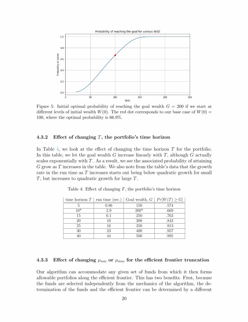
Figure 5: Initial optimal probability of reaching the goal wealth G = 200 if we start atdifferent levels of initial wealth W (0). The red dot corresponds to our base case of W (0) =100, where the optimal probability is 66.9%.

4.3.2 Effect of changing T , the portfolio’s time horizon

In Table 4, we look at the effect of changing the time horizon T for the portfolio.In this table, we let the goal wealth G increase linearly with T , although G actuallyscales exponentially with T . As a result, we see the associated probability of attainingG grow as T increases in the table. We also note from the table’s data that the growthrate in the run time as T increases starts out being below quadratic growth for smallT , but increases to quadratic growth for large T .

Table 4: Effect of changing T , the portfolio’s time horizon

time horizon T run time (sec.) Goal wealth, G Pr[W (T ) ≥ G]

5 0.86 150 .57410* 2.9 200* .66915 6.1 250 .76320 10 300 .84325 16 350 .91330 23 400 .95740 44 500 .995

4.3.3 Effect of changing µmin or µmax for the efficient frontier truncation

Our algorithm can accommodate any given set of funds from which it then formsallowable portfolios along the efficient frontier. This has two benefits. First, becausethe funds are selected independently from the mechanics of the algorithm, the de-termination of the funds and the efficient frontier can be determined by a different

20

operating team in the fund management business from the team running the dynamicprogramming algorithm. Further, if different sectors of the fund management busi-ness need to work with different funds, our algorithm can easily accommodate eachsector separately. Second, the spread in the wealth distribution at time T can becontrolled to some degree by changing the endpoints of the interval µ ∈ [µmin, µmax]that restrict the (σ, µ) pairs on the efficient frontier available to our algorithm. Inthis subsection we explore this second benefit by altering µmin and then µmax in ourbase case.

Figure 6: Graphs for the probability distribution of the terminal wealth when µmin andµmax are varied. All other parameters from the base case remain the same. The ranges are:µmin = {0.0526, 0.06, 0.065, 0.07} and µmax = {0.07, 0.0886, 0.10, 0.15}.

Recall that in our base case we consider 15 (σ, µ) pairs on the efficient frontier, withthe lower end of the frontier at (0.0374, 0.0526) and the upper end at (0.1954, 0.0886),so µmin = 0.0526 and µmax = 0.0886. In the top panel of Figure 6, we see the effecton the terminal distribution of wealth when we chose four different values for µmin:0.0526, 0.06, 0.065, and 0.07. As µmin increases, the probability of attaining the goalwealth G = 200 goes down since the interval of available controls shrinks. Also, the

21

wealth distribution has a higher variance, as is to be expected. But these higher riskdistributions also have higher positive skewness, evident from the longer right tails.Therefore, choosing the value of µmin corresponds to choosing a trade-off betweenvariance and skewness. More notably, the left tails of all three distributions are verysimilar, indicating that modulating µmin has a much stronger effect on the right sideof the wealth distribution.

The lower panel of Figure 6 shows the effect of varying µmax by considering fourdifferent µmax values: 0.07, 0.0886, 0.10, and 0.15. Again, the probability of attainingthe goal wealth G = 200 increases as µmax increases, because the interval of availablecontrols grows. However, in this case we notice that both the left and right sides ofthe probability distribution are affected, although the effect on the downside is morepronounced than that on the upside, suggesting that varying µmax has a greater effecton the left tail.

An investor that is more accepting of risk would tend to first want to increaseµmax, but Figure 6 suggests that increasing µmin might be the wiser course of action,since we can see in this case that increasing µmin appears to have a stronger influenceon the upside potential whereas increasing µmax appears to have a stronger influenceon the downside, risking significant losses without that much compensating gains.

The reason for this is actually straightforward: The algorithm is only interestedin attaining the goal wealth, so the optimal strategy for a well-off investor is to moveµ to µmin so as to reduce volatility and the chance of major losses resulting in nolonger being on track to attain the goal wealth. Because the well-off investor usesµmin, increasing µmax has little effect on the right tail, while increasing µmin has asignificant effect. Similarly, when the investor is worse off, they select µmax becausethat increases both µ and σ, which increase the chance of big gains and attaining thegoal wealth. Of course this also increases the chance of big losses, which inflates theleft tail of the wealth distribution.

4.3.4 The effect of cash flows: infusions or withdrawals

1. Annual infusions: C(t) > 0

We continue to work with our base case where we have an initial investment ofW (0) = 100 thousand dollars and a goal of having at least W (T ) = G = 200thousand dollars at the end of T = 10 years. In Table 5, we look at how constantannual infusions of C(t) = 1, 2, . . . , 9 thousand dollars affect the maximumprobability of reaching this goal, as well as the probability of reaching at least150 thousand dollars. We note from the table that even small infusions canhave a significant effect on increasing these probabilities.

2. Annual withdrawals: C(t) < 0 and the probability of going bankrupt.

We now look at the same situation, but with constant annual withdrawals in-stead of infusions, so C(t) is now a negative constant. Should the annual with-drawal amount become significant, the investor will now risk bankruptcy (i.e.,

22

Table 5: Effect of changing annual infusions, C(t) ≥ 0

value of C(t) Pr[W (T ) ≥ 150] Pr[W (T ) ≥ G = 200]

0* .777 .6691 .832 .7302 .881 .7893 .926 .8484 .961 .9015 .984 .9446 .996 .9767 .999 .9928 .999 .9989 .999 .999

W (T ) = 0). In Table 6, we see how increasing the withdrawal rate increases thechance of the investor going bankrupt, while decreasing both the probability ofreaching 150 thousand dollars and the probability of reaching the goal wealthof 200 thousand dollars at time T = 10.

Table 6: Effect of changing annual withdrawals, C(t) ≤ 0

value of C(t) Pr[W (T ) = 0] Pr[W (T ) ≥ 150] Pr[W (T ) ≥ G = 200]

0* 0 .777 .669-1 0 .720 .609-5 .002 .491 .387-10 .124 .246 .182-15 .492 .099 .072-20 .796 .034 .021-25 .937 .004 .001

4.3.5 Attaining retirement goals: our algorithm versus a target date ap-proach

Our algorithm can be used to solve a variety of important problems for optimizingretirement savings. Here, for example, we consider the effect of infusions on themaximized probability of not running out of money in retirement. In particular, weconsider at t = 0 a 50 year old investor who currently has 100 thousand dollars intheir retirement account and intends to take out 50 thousand present day dollarsevery year after they turn 65 through the age of 80, where t = T = 30. We assumethat the annual rate of inflation is 3%, so, in thousands of dollars, that means that atage 66, C(t) = −50 · 1.0316, at age 67, C(t) = −50 · 1.0317, up through age 79 whereC(t) = −50 ·1.0329. Because C(t) isn’t defined at time T , which corresponds to whenthe investor is 80, we need to set the goal wealth G equal, in thousands of dollars, toG = 50 · 1.0330 = 121.4, so that the investor can make their final withdrawal without

23

going bankrupt.

Our algorithm now optimizes the chance that the investor does not go bankrupt,but it finds, unfortunately, that this optimal probability is only 12.8%. The investor,therefore, considers making infusions of c thousand present day dollars each year untilretiring at age 65, starting with an infusion of c · 1.03 at the age of 51. The effect ofincreasing c on the maximized probability of remaining solvent at age 80 is given inthe first two columns of Table 7.

Table 7: Effect of changing pre-retirement infusions, c, for our algorithm with the goal ofstaying solvent and for our Target Date Fund

Our GBWM algorithm: Our Target Date Fund:probability of probability of

Value of c staying solvent staying solvent

0 12.8% 0.7%5 25.8% 3.9%10 42.0% 11.9%15 58.6% 26.6%20 73.5% 45.0%25 85.4% 62.7%30 93.8% 77.0%35 98.4% 86.6%40 99.8% 92.8%

Target Date Funds (TDFs) play an important role in the space of retirementinvesting. They provide a logical investment strategy that has the advantage of beingcustomized to the age of an investor. Our GBWM approach allows the investmentstrategy to be further customized to the investor’s needs by considering their goals,timeframe, cash flows, and state of wealth over time, in addition to their age.

To quantify the advantages this additional customization provides, we have, forcomparison to our GBWM results, created a hypothetical TDF using the same threeindex funds representative of U.S. Bonds, International Stocks, and U.S. Stocks usedby our GBWM algorithm, along with a typical glide path, shown in Table 8, for aninvestor transitioning from age 50 to age 80. Using the allocations from the glidepath in this table, we use simulation to determine the probabilities of an investorremaining solvent at age 80. This gives us the results shown in the Target Date Fundcolumn in Table 7.

Table 8: Our Target Date Fund glide path

Age range 50–54 55–59 60–64 65–69 70–74 75–80

1. U.S. Stock 44% 40% 35% 28% 20% 18%2. International Stock 29% 26% 23% 19% 13% 12%

3. U.S. Bond 27% 34% 42% 53% 67% 70%

24

We see from Table 7 that our algorithm shows a significantly higher ability toachieve the investor’s goal of staying solvent. More specifically, the advantage inusing our GBWM algorithm is greater than 30 percentage points when c = 10 or 15and remains high for the other values of c as well.

There are a number of reasons for our algorithm’s considerable outperformance.One reason is that the TDF retirement allocations are not generally on the effi-cient frontier, so they incur some additional volatility that is not compensated byincreased expected returns. A second reason is that the allocation within TDFs istime dependent, but does not depend on the level of the investor’s wealth, whereas ouralgorithm’s allocation strategy depends on both time and the level of wealth. Finally,our algorithm takes into account the investor’s stated goals and decisions, specificallythe infusions and the withdrawals the investor has pre-determined, as well as theinvestor’s timeframe and the goal of staying solvent at the end of this timeframe.By allowing our optimization to be customizable to an individual investor’s circum-stances, specifications, and goals, our algorithm gains a considerable advantage overthe one-size-fits-all nature of target date funds. Table 7 shows that these differencesare not small.

We can better understand the trade-offs between our GBWM algorithm and ourTarget Date Fund by comparing the two panels in Figure 7, where we present oneminus the cumulative probability distributions at t = {5, 10, 15, 20, 25, 30} years forour GBWM methodology and our Target Date Fund. For this figure we have chosenc = 15. We note that the right tail of our Target Date Fund at t = 30 is higher. Wealso note at times like t = 20 that the chance of not going bankrupt, which is thevalue of the graph at W = 0, is slightly lower for our GBWM methodology than ourTDF. These are the trade-offs that lead to our GBWM methodology attaining itsgoal of a much higher probability of not going bankrupt than our TDF (58.6% versus26.6%) at t = 30.

In Table 9, we change the goal of our algorithm from staying solvent to endingwith a balance at or above $500,000. This has no effect on our Target Date Fundnumbers, of course, but for our algorithm, as expected, it lowers the probability ofstaying solvent, while increasing the probability of ending above $500,000. Again, wesee that the advantage in using our GBWM methodology is greater than 30 percentagepoints, this time when c = 15, 20, or 25, and, again, it remains high for the othervalues of c as well. The effect of changing the GBWM goal to having a balance at orabove $500,000 on the wealth distribution over time can be seen in the top panel ofFigure 8. Note in this panel the evolution of the advantageous kink that finally landsat $500 thousand in the t = T = 30 curve.

Finally, in Table 10, we show the results of dividing our goal, as discussed inSubsection 3.3, between staying solvent with a 60% weight and ending with a balanceat or above $500,000 with a 40% weight. Comparing the results in Table 10 with theresults in Table 7, we see that having a 60% weight, as opposed to the full weight, onthe goal of staying solvent leads to losses in the probability for attaining this goal ofless than 5 percentage points, while comparing Table 10 with Table 9 for the goal of

25

Figure 7: The distribution of wealth, given as one minus the cumulative distributionfunction, as it evolves across t = {5, 10, 15, 20, 25, 30} years when the contribution level, c,is 15 from t = 1 to t = 15. The top panel depicts the wealth evolution when the goal of ourGBWM methodology is to remain solvent at T = 30. We note that wealth curve presentedfor t = T = 30 already has the final goal wealth, G = 121.4, subtracted from it, since G isto be withdrawn at T = 30. The bottom panel shows the wealth evolution for our TargetDate Fund. Comparing the two t = 30 curves at W = 0, we see the jump from 26.6% to58.6% in the probability of remaining solvent that our GBWM strategy provides, as shownin Table 7.

attaining at least $500,000, we only observe losses of less than 4 percentage points.The evolution of the distribution for this mixed GBWM goal when c = 15 can beseen in the bottom panel of Figure 8. Note that, as one would expect, we now seetwo advantageous kinks at $0 and $500 thousand in the t = T = 30 curve.

5 Concluding Discussion

In this paper, we have developed an algorithm that can quickly determine (generallywithin a few seconds to a minute) an optimal dynamic trading strategy for goals-basedwealth management (GBWM). The objective function we maximize in our GBWM

26

Figure 8: The distribution of wealth, given as one minus the cumulative distributionfunction, as it evolves across t = {5, 10, 15, 20, 25, 30} years when the contribution level, c,is 15 from t = 1 to t = 15. The top panel depicts the wealth evolution when the goal of ourGBWM methodology is to deliver an amount greater than $500,000 at T = 30. The bottompanel displays the wealth evolution when we split the goal for our GBWM methodologybetween staying solvent with a 60% weight and delivering an amount greater than $500,000with a 40% weight at T = 30. In both panels, the wealth curve presented for t = T = 30already has the final goal wealth, G = 121.4, subtracted from it, since G is to be withdrawnat T = 30.

framework is the probability of reaching a given goal wealth at the end of a giveninvestment horizon, in contrast to maximizing the expected utility of the wealth atthe end of a given time horizon. Without any sacrifice in runtime, our algorithmcan optimally allocate from among any given set, large or small, of chosen portfolios,which can be determined outside of our algorithm. Also, without any sacrifice inruntime, our algorithm can accommodate periodic specified infusions or withdrawals.Further, we can easily compute the probability of running out of money at each perioddue to any of these withdrawals.

The dynamic programming approach, whose computation works backwards intime, has important advantages over approaches that work forwards in time. Dy-namic programming addresses the fact that the optimal portfolio allocation will shift

27

Table 9: Effect of changing pre-retirement infusions, c, for our algorithm with the goal ofending with at least $500,000 and for our Target Date Fund

Our algorithm: Our Target Date Fund:probability of ending probability of ending

Value of c with ≥ $500,000 with ≥ $500,000

0 8.9% 0.2%5 18.5% 1.2%10 31.2% 4.2%15 45.1% 12.0%20 58.7% 24.5%25 70.9% 39.9%30 81.2% 55.6%35 89.2% 69.5%40 94.9% 80.1%

Table 10: Effect of changing pre-retirement infusions, c, for our algorithm with the splitgoal of staying solvent with a 60% weight and ending with at least $500,000 with a 40%weight.

Our algorithm: Our algorithm:probability of probability of ending

Value of c staying solvent with ≥ $500,000

0 11.8% 8.1%5 23.8% 16.9%10 38.9% 28.8%15 54.5% 42.2%20 68.7% 55.5%25 80.5% 67.8%30 89.5% 78.5%35 95.6% 87.2%40 98.8% 93.8%

over time. Attempting to consider this with a forwards in time algorithm is computa-tionally infeasible, so these algorithms are reduced to myopic approaches, where theallocation chosen at a point in time is only optimal under the assumption that nofurther reallocation will occur. That is, the forwards in time algorithms are restrictedto the inferior approach of repeated static optimization. Interestingly, despite this,the results from the repeated static optimization method described in Das, Ostrov,Radhakrishnan, and Srivatav (2018) end up being very similar to the results obtainedfrom our dynamic programming approach, however, that paper’s method, which re-lies on the solution to a stochastic differential equation (SDE), cannot be extendedto infusions or withdrawals and it has a longer computational time. Most forwardsin time approaches rely on simulation instead of solving an SDE, which leads to evenlonger computational times to be reasonably accurate.

We can modulate the left and right tails of the terminal wealth distribution by

28

varying the chosen range of allowable portfolios on the efficient frontier. If we removeeither the most risky investments at the top of this range or the least risky investmentsat the bottom of this range, we lower the probability of reaching our goal wealth, sincewe are restricting the set of controls available to the algorithm. However, removingthe most risky investments has the benefit of lowering the left tail in the distribution,as it lowers the chance of significant losses, while removing the least risky investmentshas the benefit of raising the right tail in the distribution, making it more likely toattain wealth values that are significantly higher than the goal wealth.

Target date (or life-cycle) funds have the important feature of being able to re-allocate funds based on time, specifically on the age of the investor. They cannot,however, reallocate based on the investor’s wealth or the investor’s specific goals.Nor are the allocations underlying a target date fund necessarily on the efficient fron-tier. The natural question arises as to weather incorporating these GBWM featuresand efficiency constraints, which require individualized attention through automationand/or human advisors, adds much value to the investor. Our paper concludes thatthey can actually add considerable value. We explored the case of a 50 year old savingfor retirement at age 65, who then takes out inflation adjusted withdrawals until theage of 80. Working with just three index funds representative of U.S. Bonds, Inter-national Stocks, and U.S. Stocks, we show examples where our algorithm’s optimaldynamic reallocation strategy increases the chance of this investor remaining solventat age 80 by more than 30 percentage points over using a Target Date Fund duringthis period.

The approach in this paper can be expanded to answer questions arising in otherimportant financial situations. These include incorporating the effect of taxes or in-corporating stochastic efficient frontier models. Because our algorithm runs so quickly,it is unlikely that these additional features will degrade the runtime particularly sig-nificantly.

Authors

Sanjiv Das is the William and Janice Terry Professor of Finance and Data Sciencein the Leavey School of Business at Santa Clara University.

Dan Ostrov is a Professor of Mathematics and Computer Science at Santa ClaraUniversity.

Anand Radhakrishnan is a Client Analytics Director within the Client Strategiesand Analytics group at Franklin Templeton Investments.

Deep Srivastav is a Senior Vice President and heads the Client Strategies andAnalytics group at Franklin Templeton Investments.

29

References

Birge, J.R., and F.V. Louveaux, (1997). Introduction to Stochastic Programming.Springer Verlag, New York.

Browne, S. (1995). Optimal investment policies for a firm with a random risk pro-cess: Exponential utility and minimizing the probability of ruin. Mathematics ofOperations Research 20(04), 937-958.

Browne, S. (1997). Survival and growth with a liability: Optimal portfolio strategiesin continuous time. Mathematics of Operations Research 22(02), 468-493.

Browne, S. (1999a). Reaching goals by a deadline: Digital options and continuous-time active portfolio management. Advances in Applied Probability 31(02), 551-577.

Browne, S. (1999b). The risk and rewards of minimizing shortfall probability. TheJournal of Portfolio Management 25(04), 76-85.

Browne, S. (2000). Risk-constrained dynamic active portfolio management. Manage-ment Science 46(09), 1188-1199.

Brunel, J.L.P., (2015). Goals-Based Wealth Management: An Integrated and PracticalApproach to Changing the Structure of Wealth Advisory Practices, Wiley & Sons,New Jersey.

Chhabra, Ashvin., (2005). Beyond Markowitz: A Comprehensive Wealth AllocationFramework for Individual Investors, Journal of Wealth Management, Spring, 8-34.

Cox, J.C., and Chi-fu Huang (1989). Optimal consumption and portfolio policieswhen asset prices follow a diffusion process, Journal of Economic Theory 49(1),33-83.

Das, S.R., H. Markowitz, J. Scheid, M. Statman, (2010). Portfolio Optimization withMental Accounts, Journal of Financial and Quantitative Analysis 45(2), 311-334.

Das, S.R., D. Ostrov, A. Radhakrishnan, D. Srivastav (2018). Goals-Based WealthManagement: A New Approach, Journal of Investment Management 16(3), 1-27.

Deguest, R., L. Martellini, V. Milhau, A. Suri, H. Wang, (2015). Introducing aComprehensive Risk Allocation Framework for Goals-Based Wealth Management,EDHEC-Risk Institute.

Kahneman, D. and A. Tversky (1979). Prospect Theory: An Analysis of Decisionunder Risk, Econometrica 47, 263-291.

Lopes, L. (1987). “Between Hope and Fear: The Psychology of Risk.” Advances inExperimental Social Psychology 20, 255-295.

Markowitz, H., (1952). Portfolio Selection, Journal of Finance 6, 77-91.

30

Merton, R.C. (1969). Lifetime Portfolio Selection under Uncertainty: TheContinuous-Time Case, The Review of Economics and Statistics 51(3), 247-257.

Merton, R.C. (1971). Optimum consumption and portfolio rules in a continuous-timemodel, Journal of Economic Theory 3(4), 373-413.

Nevins, Daniel., (2004). Goals-Based Investing: Integrating Traditional BehavioralFinance, Journal of Wealth Management 6, 48-23.

Roy, A.D., (1952). Safety-first and the Holding of Assets, Econometrica 20, 431-449.

Shefrin, H.M. and M. Statman., (1985). The disposition to sell winners too early andride losers too long: Theory and evidence, Journal of Finance 40, 777-790.

Shefrin, H.M. and M. Statman., (2000). Behavioral Portfolio Theory, Journal of Fi-nancial and Quantitative Analysis 35(2), 127-151.

Thaler, R.H. (1985). Mental Accounting and Consumer Choice, Marketing Science 4,199-214.

Thaler, R.H. (1999). Mental Accounting Matters, Journal of Behavioral DecisionMaking 12, 183-206.

Wallace, S.W. and W.T. Ziemba (eds.) (2005). Applications of Stochastic Program-ming. MPS-SIAM Book Series on Optimization.

Wang, H., A. Suri, D. Laster, H. Almadi (2011). Portfolio Selection in Goals-BasedWealth Management, Journal of Wealth Management 14(1), 55-65.

31