Dynamic pricing of inventory/capacity with infrequent

price changes

Serguei Netessine∗

The Wharton School

University of Pennsylvania

Philadelphia, PA 19104-6366

netessin@wharton.upenn.edu

Spetember 2003, Revised July 2004, December 2004

Forthcoming in European Journal of Operational Research

Abstract

We consider a problem of dynamically pricing a single product sold by a monopolist over a short time

period. If demand characteristics change throughout the period, it becomes attractive for the company to

adjust price continuously to respond to such changes (i.e., price-discriminate intertemporally). However,

in practice there is typically a limit on the number of times the price can be adjusted due to the high

costs associated with frequent price changes. If that is the case, instead of a continuous pricing rule the

company might want to establish a piece-wise constant pricing policy in order to limit the number of price

adjustments. Such a pricing policy, which involves optimal choice of prices and timing of price changes,

is the focus of this paper.

We analyze the pricing problem with a limited number of price changes in a dynamic, deterministic

environment in which demand depends on the current price and time, and there is a capacity/inventory

constraint that may be set optimally ahead of the selling season. The arrival rate can evolve in time

arbitrarily, allowing us to model situations in which prices decrease, increase, or neither. We consider

several plausible scenarios where pricing and/or timing of price changes are endogenized. Various notions

of complementarity (single-crossing property, supermodularity and total positivity) are explored to derive

structural results: conditions sufficient for the uniqueness of the solution and the monotonicity of prices

throughout the sales period. Furthermore, we characterize the impact of the capacity constraint on the

optimal prices and the timing of price changes and provide several other comparative statics results.

Additional insights are obtained directly from the solutions of various special cases.

Keywords: Pricing; Economics; Complementarity; Menu Costs.

∗The author is grateful to Gerard Cachon, Jiri Chod, Pranab Majumder, Nils Rudi and Rober Shumsky for discussions

and helpful comments on the earlier versions of this paper. The comments of three anonymous referees helped to improve and

streamline the paper.

1

1 Introduction

Price discrimination by the time of purchase is a standard practice in many industries. A person eager to

buy a new designer suit will pay a much higher price early in the season whereas a person who is not so eager

will pay a much lower price at the end of the season. On the other hand, customers buying airline tickets

far in advance are typically more price sensitive than those who make their purchases at the last minute.

In both of these cases companies can benefit from the use of intertemporal price discrimination (dynamic

pricing) but, due to particular customer preferences, industry-specific pricing policies differ significantly1.

An attractive way to price-discriminate is to change the price continuously over time by reacting to any shifts

in demand characteristics. However, such a practice is often either not feasible or too costly. In the airline

industry, for example, reservation system limitations do not allow for continuous price changes even though

airlines do change prices quite frequently. In other cases (including, for example, cruise line operation and

theaters), the sale is made through a network of agents with prices pre-printed in catalogs, which makes

price adjustments costly. A similar problem is faced by catalog retailers who incur significant costs each

time prices change and new catalogs have to be printed. In the general retail setting each price decrease is

communicated to customers by means of advertising and hence, again, significant costs are incurred each

time prices are adjusted. Zbaracki et al. [33] cite the case of a large industrial manufacturer spending more

than $1M per year to administer price changes (20% of the net margin). Sometimes there is also a fear of

antagonizing customers through too frequent price changes. For all these reasons, in a variety of practical

situations companies change prices only a limited number of times throughout the sales period. Empirical

evidence of the high costs associated with price adjustments is plentiful: see, for example, Levi et al. [20]

for supermaket chains, Levi et al. [21] for multiproduct retailers and Zbaracki et al. [33] for industrial

manufacturers. Yet, studies that link cost of price changes to dynamic pricing policies are scarce. Recent

advances in e-commerce and information systems have decreased the costs of price changes (see Brynjolfsson

and Smith [6]) making them less of an issue in electronic commerce. However, there is still a long way to go

before this innovation is adopted in areas like brick-and-mortar retailing and moreover, customer antagonism

to frequent price changes will still remain even in e-commerce. As we will demonstrate, correctly identifying

the optimal pricing policy when only a limited number of price changes are allowed may be more complex

than identifying the optimal pricing policy in the absence of this limitation.

A whole separate stream of economics literature studies price stickiness, a phenomenon in which firms some-

times try to avoid changing prices frequently due to the costs (often called “menu costs”) associated with

such changes. Zbaracki et al. [33] provide a survey of the relevant literature and give empirical evidence

of the large magnitude of menu costs in the industrial setting. In particular, they separate out three cost

components: physical (e.g., changing price labels), managerial (including information-gathering, decision-

making and communication costs), and customer (including negotiation and communication costs) and find

1Companies can also benefit from dynamic pricing policies because of the stochastic nature of demand. This aspect of

dynamic pricing is outside of the scope of this paper. However, in the stochastic setting our results can be used heuristically in

a rolling-horizon mode using the certainty equivalent formulation.

2

that managerial and customer costs are orders of magnitude larger than the direct physical costs associated

with price changes.

This paper focuses on two issues that arise when a firm uses intertemporal price discrimination with a limited

number of price changes: how to price the product on each time interval when the price is fixed and when

to switch from one price to the other. In our model, customers arrive continuously at a deterministic rate

that is a function of time and current price. By assuming that the functional form of the arrival rate is

an almost entirely arbitrary (price and time-dependent) function, we combine in one paper the analysis of

situations in different industries in which an optimal pricing policy is monotonically increasing (as is typical

for airlines), monotonically decreasing (as is typical in fashion retailing) or neither. Moreover, in addition to

situations in which capacity is not a constraint (e.g., production-to-order), we analyze situations in which

capacity/inventory can be a constraint (e.g., some fashion retail situations and service applications includ-

ing airlines, hotels, performance events) that may be set optimally at the commencement of the selling season.

Several scenarios are considered in this paper. We begin our analysis by assuming that a set of allow-

able prices is given exogenously (e.g., due to competitive considerations) and show that the timing of price

changes may be complicated by the presence of multiple local minima and maxima and provide intuition as

to why this is the case. Regularity conditions that ensure various degrees of complementarity — the single-

crossing property, total positivity and supermodularity — between the pricing and the timing components of

the demand function are shown to be sufficient for the uniqueness of the timing solution. The very same

conditions help characterize situations in which a monotone price increase/decrease throughout the sales

period is optimal and also allow us to determine the impact that the change in one of the prices will have

on the optimal timing of price changes. A surprising result here is that, due to the limited number of price

changes, the optimal timing of price changes can increase or decrease in price, depending on the comparison

between the price that is set on a given time interval and the optimal continuous price. Finally, we show

that the optimal timing is a monotone function of capacity.

We then turn to the situation in which the pricing decision is endogenized but the timing of price adjustments

is exogenously specified (e.g., the timing of price changes coincides with holidays). We provide conditions

sufficient for the uniqueness of the pricing decision and characterize the impact of exogenous changes in

timing on optimal prices. We also show that all prices are monotone in the capacity constraint. If in either

scenario the capacity can be set optimally before the season begins, we show that there is a unique solution

to the capacity problem. Finally, we analyze the problem of jointly setting timing, pricing, and capacity.

We show that, if the revenue rate function is Totally Positive of Order 2, then the pricing policy is monotone

throughout the sales period regardless of the timing and capacity decisions. To gain further insights into the

problem, we introduce a simplifying assumption in order to separate shifts in customer price sensitivity from

changes in demand intensity, thus making the problem more transparent. Closed-form solutions for pricing

and capacity decisions are obtained, and many of the results derived for the general form of the arrival rate

function are illustrated. In particular, we demonstrate how the timing of price changes can differ depending

on the functional form of the demand function. We also address the issue of optimal capacity selection and

3

find that, in this simplified problem, the capacity decision can be made without advanced knowledge of the

price discrimination policy. Hence, as opposed to many situations described in the literature, marketing

and operations functions within the firm can be separated so that the firm does not need to commit to a

specific pricing scheme at the time of the capacity decision. The separability of the pricing and inventory

decisions is a useful insight since these decisions are usually made at different points in time. In conclusion,

we consider examples illustrating the losses that accrue from an insufficient number of price changes.

2 Relation to the literature

While continuous dynamic pricing problems have received extensive treatment in the literature, the variant of

the same problem with only a limited number of price changes has been investigated less frequently. Research

in relevant areas spans streams of papers in economics, marketing, and operations management with many

papers incorporating both pricing and operational decisions (production/inventory policy). Economists

coined the term “intertemporal price discrimination” to describe discriminatory pricing based on the time of

purchase (see survey by Varian [31]). Research in this area is rather sparse, with the main focus on analyzing

price discrimination from the social welfare point of view. The earliest papers in this stream consider the

problem of pricing durable goods (i.e., products that create secondary markets) over time. See Coase [9]

and Bulow [7] for the corner stone work on durable goods.

In marketing there is a large stream of literature on pricing (see a comprehensive survey by Rao [28]) with

the most relevant papers modeling pricing as a dynamic continuous decision. This stream includes models

that may account for consumer behavior, competition, and other factors, with many papers focusing specif-

ically on markdowns. A related set of papers looks at the intertemporal price discrimination that occurs

when price declines as time progresses and consumers anticipate this decline and react to it by delaying

their purchase (see summary and citations in Lilien et al. [23], page 187). This setting is different from

our work since we do not focus on the price decrease alone and instead consider more general situations in

which prices may increase, decrease or neither. “Gaming” behavior by the customers (e.g., delayed purchase

or buying tickets for resale later) is an interesting aspect of the dynamic pricing problem and one that is

typically omitted from the dynamic pricing literature. Although it is beyond the scope of our work, we

acknowledge this limitation and hope that it can be addressed in future work. Levinthal and Purohit [22]

consider intertemporal pricing in the context of the durable goods problem when the product becomes ob-

solete over time due to introduction of a superior product. Eliashberg and Steinberg [10] investigate joint

pricing/inventory decisions when price can be adjusted continuously. The work of Rajan et al. [27] consid-

ering pricing of the product that is subject to value drop is particularly relevant since, similar to our model,

it analyzes the problem with the single-ordering decision at the commencement of the season and dynamic

pricing throughout the season. Additionally, the optimal timing of the length of the season is a decision

variable that is somewhat related to the optimal timing of multiple price changes in our paper. However,

the price in their paper can be adjusted continuously, which is different from our work.

In the operations management literature price discrimination/dynamic pricing has been studied in sev-

4

eral contexts using both stochastic and deterministic models of customer demand (models in market-

ing/economics are predominantly deterministic). Although the deterministic demand assumption is, ad-

mittedly, a major simplification, there are several reasons to consider deterministic models (see Bitran and

Caldentey [4] for details). First, deterministic models are easier to analyze and they often provide good

approximations for stochastic models. Hence, deterministic models can provide valuable insights, especially

on the way various parameters impact pricing policies. Second, deterministic solutions are typically optimal

asymptotically. Finally, deterministic models are widely used in practice. Among papers using deterministic

demand, Kunreuther and Schrage [19] is one of the early papers on this topic and work of Gallego [15], Gupta

et al. [17] and Smith and Achabal [29] are most closely related to ours. Gallego [15] develops a dynamic

deterministic model to analyze timing and pricing in the problem with price-dependent arrival rate, one price

change and two streams of customers: one for low-fare and one for high-fare tickets (we have a common

stream of customers). Gupta et al. [17] develop a deterministic pricing model (and also present stochastic

extension) with an arbitrary number of price changes and a specific (multiplicative) form of the arrival rate

function. Among other results, they show that if price sensitivity of customers is monotonically increasing,

it is optimal to decrease price throughout the season. Our analysis generalizes this result by characterizing

situations in which price decrease/increase is optimal for a more general form of the arrival rate function.

Smith and Achabal [29] assume that the demand depends on both price and current inventory and, similar

to our work, show that the optimal inventory/capacity selection is independent of the price trajectory. In

their setting it may be optimal to have a non-zero ending inventory.

Research on dynamic pricing in stochastic settings is surveyed by Elmaghraby and Kesinocak [11], Chan et

al. [8], Bitran and Caldentey [4] and McGill and van Ryzin [24]. Papers in this stream model customer ar-

rivals as a Poisson process, allowing an unlimited number of price changes. The closest papers in this stream

also consider situations in which there is a pre-determined set of allowable prices (so that only the timing

of price changes is a decision) or, alternatively, in which the timing of price changes is pre-determined but

prices are set optimally. Most papers in this stream assume that the customer arrival rate is time-invariant

while we do not impose such a restriction. Gallego and van Ryzin [16] show that charging a single deter-

ministic price is asymptotically optimal in this setting, a result that we confirm and generalize. Bitran and

Mondschein [5] analyze both continuous pricing and a policy with a limited, pre-determined number of price

changes. However, the timing of these price changes is not a decision variable in their model. They find that

the expected revenue varies significantly in the number of price changes. Feng and Gallego [13] consider a

situation in which only one price change is allowed (while we allow multiple changes). As in our paper, the

timing of the price change is a decision variable but prices are pre-specified. To derive regularity condition,

they utilize a notion of complementarity. Zhao and Zheng [34] were, perhaps, the first to relax the time-

invariance of the arrivals assumption. They allow for continuous price changes and derive a condition that is

sufficient for monotonicity of prices. We show that this condition is also sufficient when the number of price

changes is limited, and we link this condition to notions of complementarity. In a similar setting, Feng and

Gallego [14] consider the problem of switching among multiple pre-determined prices (in our problem prices

can be decision variables). They cite difficulties in deriving conditions sufficient for monotonicity of prices.

We find such conditions in a setting with deterministic arrival rate. Aviv and Pazgal [1] numerically analyze

5

the impact of the number of price changes on the dynamic pricing policy and find that the optimal profit

is concave increasing in the number of allowed price changes and moreover, the benefits from having more

price changes are decreasing with the increase in product inventory. Other papers in this stream analyze

the problem of pricing dynamically multiple products. A different stream of research analyzes simultaneous

pricing/inventory control problem in which there are multiple price changes but the timing of these changes

is not a decision variable (see Federgruen and Heching [12]).

To summarize, this paper makes three primary contributions. Our first contribution is in analyzing the

dynamic pricing problem with a limited number of price changes and providing insights into pricing and

timing decisions. Most of the related papers either allow for continuous price changes or assume that the

firm operates in a multiple-period environment with time-invariant demand characteristics in each period.

The former assumption differs from our work since we assume that the number of times price can be changed

is limited, which is important when there are costs associated with each change. The latter assumption also

differs from our work since we model demand during the period as a more general time-dependent continuous

process. Our second contribution is that instead of focusing on a specific price trajectory, we employ a

more general model with a minimal number of assumptions that can incorporate both price increases and

decreases and establish when one or the other situation arises, thus making the results applicable to a variety

of industries. In some instances these assumptions are shown to be necessary and sufficient and thus cannot

be further relaxed. Finally, we contribute to the methodology by demonstrating the connection between

various notions of complementarity and structural properties of the solution to the dynamic pricing problem.

While previous papers have identified some similar structural results, none, to our knowledge, connects them

to the notions of complementarity between price and time components of the arrival rate function. The rest

of the paper is organized as follows. We first outline our model, assumptions and limitations in Section 3.

In Section 4 we conduct in-depth analysis of the problem with a limited number of price changes. To gain

additional insights, in Section 5 we introduce simplifying assumptions that make the model more transparent

and derive additional results. The paper ends with a discussion of the results in Section 6. Throughout the

presentation, several simple illustrative examples are given to enhance the reader’s intuition.

3 Model setup

Consider a monopolistic company that commits to selling products (or tickets) during the time period

t = [0, 1] where t = 1 is the event symbolizing the end of sale (airplane departure, start of the movie, end

of the selling season). Equivalently, we can assume that there are multiple identical time periods with the

same demand characteristics during each period due to, e.g., seasonality. During the selling period customers

willing to purchase the product at price p arrive dynamically at a rate λ(t, p), that is, demand is a continuous

function of price and time, while the decision to purchase or not purchase the product is based solely on the

current price. This model can incorporate, for example, uncertainty in customer reservation prices. Specif-

ically, suppose there is a known distribution of customer reservation prices v, F (t, p) = Pr(v < p|t), andcustomers arrive at a price-invariant rate λ(t) so that, from the company’s point of view, customers who make

the purchase arrive at a rate λ(t, p) = λ(t) (1− F (t, p)). Note that we preclude the arbitrage opportunity:

6

there is no way for customers to buy products for resale later and customers are also not allowed to “wait”

for a lower price (even though this may be the case in practice). In this sense, the decision to buy or not

buy is instantaneous (or myopic), i.e., like most papers addressing the issue of intertemporal price discrimi-

nation we abstract away from considering customer “gaming” behavior that is beyond the scope of the paper.

We use subscripts to denote partial derivatives and underscore to denote vectors. For simplicity, we abuse

mathematical notation somewhat, e.g., by writing λp(t, p∗), which means that the first derivative w.r.t.

price is evaluated at p∗. We assume that λ(t, p) ≥ 0 is a differentiable function that is non-increasing in p,λp(t, p) ≤ 0. Further, we require that the revenue rate function defined as pλ(t, p) be concave in p for anyt, i.e., 2λp(t, p) + pλpp(t, p) < 0. For example, any λ(t, p) concave in p satisfies this requirement, but some

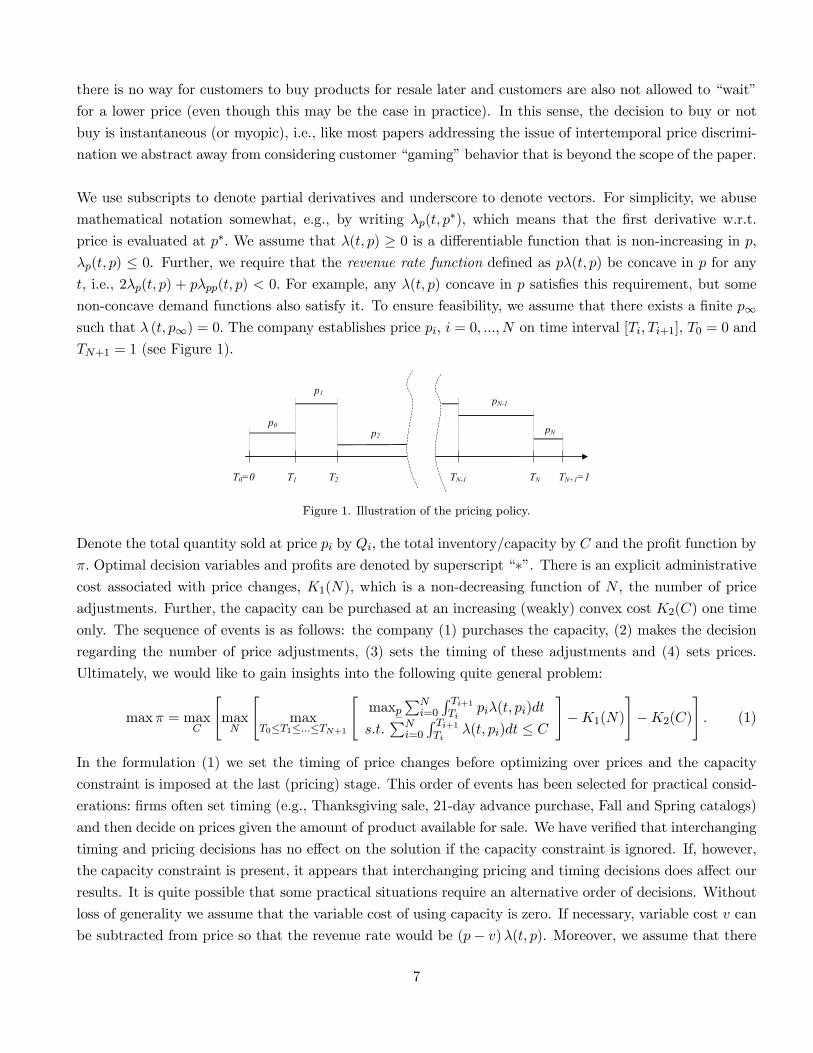
non-concave demand functions also satisfy it. To ensure feasibility, we assume that there exists a finite p∞such that λ (t, p∞) = 0. The company establishes price pi, i = 0, ..., N on time interval [Ti, Ti+1], T0 = 0 and

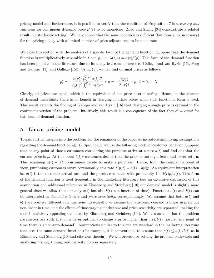
TN+1 = 1 (see Figure 1).

T0=0 T1 T2 TN-1 TN TN+1=1

p0

p1

p2

pN-1

pN

Figure 1. Illustration of the pricing policy.

Denote the total quantity sold at price pi by Qi, the total inventory/capacity by C and the profit function by

π. Optimal decision variables and profits are denoted by superscript “∗”. There is an explicit administrativecost associated with price changes, K1(N), which is a non-decreasing function of N , the number of price

adjustments. Further, the capacity can be purchased at an increasing (weakly) convex cost K2(C) one time

only. The sequence of events is as follows: the company (1) purchases the capacity, (2) makes the decision

regarding the number of price adjustments, (3) sets the timing of these adjustments and (4) sets prices.

Ultimately, we would like to gain insights into the following quite general problem:

maxπ = maxC

"maxN

"max

T0≤T1≤...≤TN+1

"maxp

PNi=0

R Ti+1Ti

piλ(t, pi)dt

s.t.PNi=0

R Ti+1Ti

λ(t, pi)dt ≤ C

#−K1(N)

#−K2(C)

#. (1)

In the formulation (1) we set the timing of price changes before optimizing over prices and the capacity

constraint is imposed at the last (pricing) stage. This order of events has been selected for practical consid-

erations: firms often set timing (e.g., Thanksgiving sale, 21-day advance purchase, Fall and Spring catalogs)

and then decide on prices given the amount of product available for sale. We have verified that interchanging

timing and pricing decisions has no effect on the solution if the capacity constraint is ignored. If, however,

the capacity constraint is present, it appears that interchanging pricing and timing decisions does affect our

results. It is quite possible that some practical situations require an alternative order of decisions. Without

loss of generality we assume that the variable cost of using capacity is zero. If necessary, variable cost v can

be subtracted from price so that the revenue rate would be (p− v)λ(t, p). Moreover, we assume that there

7

is no salvage value of inventory/capacity. This assumption is, again, without loss of generality because in

a deterministic model like ours capacity would always be set so that it is exhausted. If, however, capacity

is not a decision variable but is instead specified exogenously then the salvage value s can still be added as

long as p ≥ s so that it is always more profitable to sell than to salvage, a plausible assumption.

In (1) we have a rather complex non-linear mixed-integer programming problem that consists of four sequen-

tial optimizations. Understandably, the greatest complexity lies in establishing the structural properties of

the optimization problem with respect to N since it involves solving an integer program given that cost

function K1(N) can take almost any form. For example, an information system is often needed to effectively

support price changes (e.g., reservation systems in the case of airlines, digital price labels in retail). Hence,

K1(N) has a large fixed and a small incremental component, meaning that once the decision has been made

to purchase the information system, price changes become close to costless (except for the implicit costs

due to possible conflicts with customers). One can see then that there could be two local maxima: do

not purchase the system and establish a single price (N = 0) or purchase the system and adjust the price

continuously (N = ∞). Bitran and Caldentey [4] summarize solutions for the above model when N = 0

and N = ∞. These solutions provide, correspondingly, a lower and an upper bound for the optimal profit.Bitran and Caldentey [4] show that there is a unique optimal solution to the pricing problem, that the

optimal price is non-increasing in the capacity constraint and that there is a unique solution to the capacity

problem. As we discussed earlier, the solution with N = 0 may not be economical and the solution with

N = ∞ is sometimes undesirable in practice. This motivates our next effort, which is to consider a finite

number of price changes, an approach that provides a trade-off between the desire to price discriminate and

the complexity involved in administering continuous pricing.

4 Partial price discrimination (0 < N <∞)Increasing the number of price changes allows a company to increase profit from its lower bound (the no

price discrimination case) towards its higher bound (the perfect price discrimination case). If price changes

are costly, the firm faces a trade—off. In many practical situations the resulting number of price changes

will be rather small so that the optimal N can be found through complete enumeration. Examples include

catalog companies (with two to four catalogs per year), retail companies (with a few major sales events

tied to holidays, e.g., Thanksgiving, Christmas) and airline companies (with 21-, 14- and 7-day advanced

purchases). Hence, to simplify the problem and achieve some transparency in the analysis, we eliminate

the integer programming part of the problem by assuming for most of the paper that the number of price

changes N is known. The issue of selecting the number of price changes optimally is addressed in the last

section.

4.1 Exogenous set of prices

We first consider a situation in which prices are not decision variables but rather a set of allowable prices is

exogenously given, possibly due to some strategic considerations. Such a problem has received considerable

8

attention in the literature since firms sometimes restrict prices to a limited discrete set (see Gallego and van

Ryzin [16], Feng and Gallego [13], Feng and Gallego [14]). Suppose that the set of admissible prices P is

given exogenously (but the order of prices is not prescribed) and the total number of prices in P is N + 1,

i.e., the cardinality of P is N + 1. We assume that each price in P can be used only once but if the same

price has to be used more than once then it should be included in the set several times. This assumption is

needed to avoid the complication arising if the number of prices does not match the number of price changes

so that some prices or price changes have to be eliminated. To simplify the problem further, assume for

the time being that there is no capacity constraint (for example, the product can be produced to order as

customers arrive and there is ample production capacity) so that the objective function is

maxπ = maxT0≤T1≤...≤TN+1

NXi=0

Z Ti+1

Ti

piλ(t, pi)dt,

s.t. p ∈ P.

Notice that the order of prices is still a decision variable. In order to determine the optimal order of prices

in general (i.e., without further assumptions about the arrival rate function), it is necessary to enumerate

all (N+1)! possible permutations of prices. However, to gain further intuition, assume for the time being

that we know the order of prices. To characterize the optimal T = (T1, ..., TN ) , we obtain the first-order

necessary optimality conditions:

∂π

∂Ti= pi−1λ(Ti, pi−1)− piλ(Ti, pi) = 0, i = 1, ...,N. (2)

A casual analysis of the expression (2) suggests that even in this greatly simplified problem many reasonable

functional forms of λ(t, p) will result in multiple stationary points. To give just one example, suppose that

λ(t, p) = a(t)− p so that (2) is equivalent to

a(Ti) = pi−1 + pi, i = 1, ...,N.

If we now take any a(t) that crosses the line pi−1 + pi several times on [0, 1] , we obtain multiple stationarypoints that can be local minima and maxima.

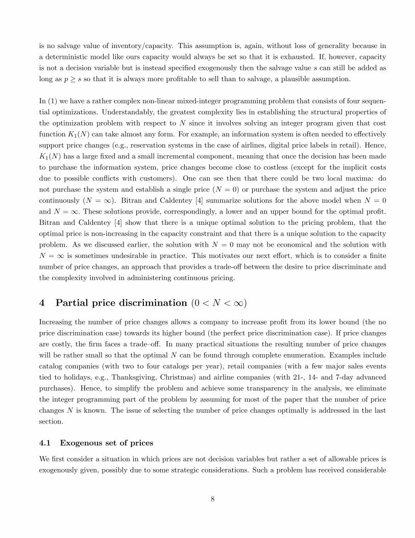
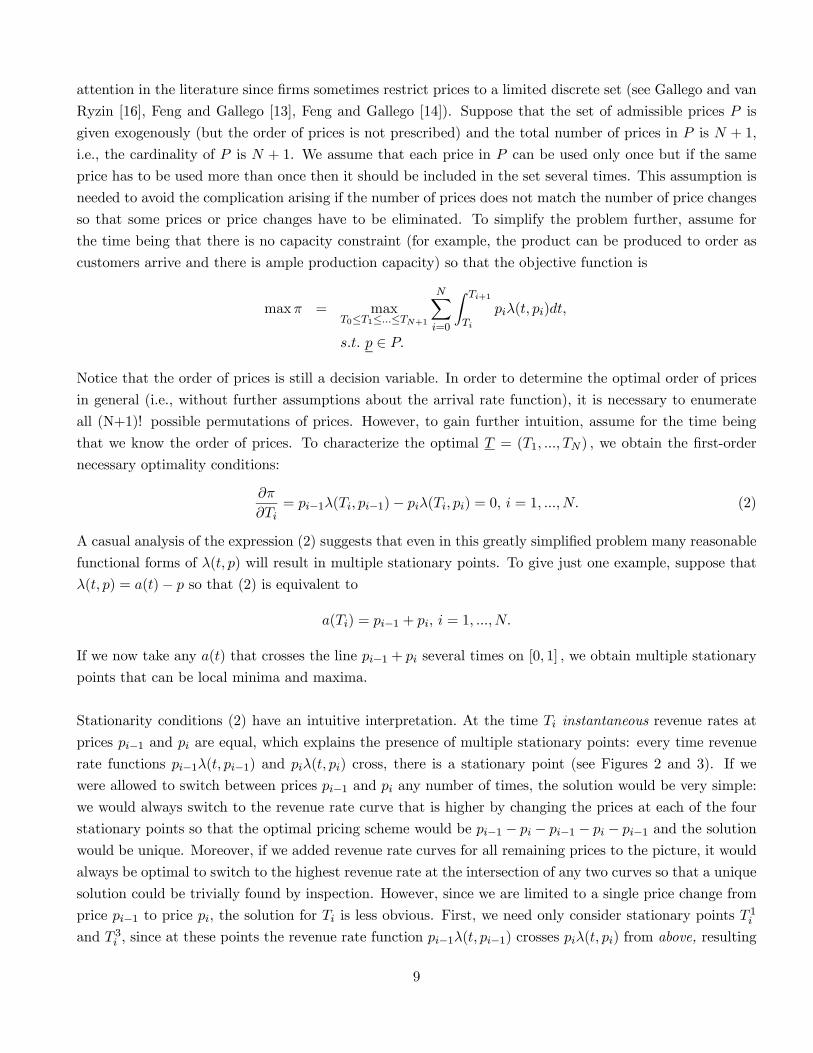
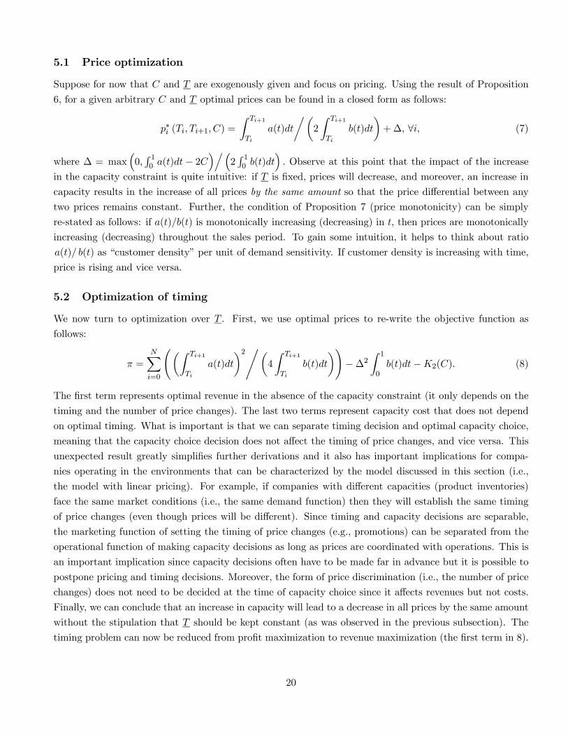
Stationarity conditions (2) have an intuitive interpretation. At the time Ti instantaneous revenue rates at

prices pi−1 and pi are equal, which explains the presence of multiple stationary points: every time revenuerate functions pi−1λ(t, pi−1) and piλ(t, pi) cross, there is a stationary point (see Figures 2 and 3). If wewere allowed to switch between prices pi−1 and pi any number of times, the solution would be very simple:we would always switch to the revenue rate curve that is higher by changing the prices at each of the four

stationary points so that the optimal pricing scheme would be pi−1 − pi − pi−1 − pi − pi−1 and the solutionwould be unique. Moreover, if we added revenue rate curves for all remaining prices to the picture, it would

always be optimal to switch to the highest revenue rate at the intersection of any two curves so that a unique

solution could be trivially found by inspection. However, since we are limited to a single price change from

price pi−1 to price pi, the solution for Ti is less obvious. First, we need only consider stationary points T 1iand T 3i , since at these points the revenue rate function pi−1λ(t, pi−1) crosses piλ(t, pi) from above, resulting

9

in the local maxima. The next step after identifying local maxima T 1i and T3i would be computing and

comparing profits at these stationary points; we might actually need to compute profits at all the stationary

points or use the second-order conditions to find local maxima.

t

Revenue rate

10

( )11 , −− ii ptp λ

( )ii ptp ,λLocal maxima

Local minima

1iT 2

iT 3iT 4

iT

Figure 2. Illustration of multiple intersections.

),(),( 11 iiiiii pTppTp λλ −−−

t

iT∂∂π

1iT 2

iT 3iT 4

iT 10

),(),( 11 iiiiii pTppTp λλ −−−

t

iT∂∂π

1iT 1iT 2

iT 2iT 3

iT 3iT 4

iT 4iT 10

Figure 3. Illustration of multiple stationary points.

It turns out that when a set of prices is exogenously given it is possible to ensure that there is both a unique

optimal order of prices and a unique timing solution by satisfying some rather mild technical requirements

that do not rely on any assumptions about the first or second derivatives of λ(t, p) (and hence do not require

monotonicity or concavity) so that they can be applied to a variety of problems. To do so it is desirable to

be able to recognize situations in which there is only a single stationary point that is also the maximum.

Clearly, from looking at Figure 2, we need a condition guaranteeing that revenue rate functions cross only

once. We now introduce the adequate machinery.

Definition 1 (Milgrom and Shannon [25]). Function f(x, y) satisfies the single-crossing property (SCP) in

(x, y) if for x0 ≥ x and y0 ≥ y, f(x0, y) ≥ f(x, y) implies that f(x0, y0) ≥ f(x, y0).

The SCP essentially means weak complementarity between x and y: the higher value of x paired with the

higher value of y dominates the lower value of x. The SCP is used in economics primarily to show para-

metric monotonicity results (as we will explain shortly) but in our particular problem the SCP also helps

ensure uniqueness of the solution. A convenient feature of the SCP is that it is preserved under increasing

transformation. For example, if we know that g(·) is an increasing function and f(x, y) satisfies the SCP,then g(f(x, y)) satisfies it as well. The power of the SCP is that it is the weakest condition that guarantees

uniqueness of the solution as well as monotonic order of prices. In other words, it is impossible to further

relax this condition in Proposition 1 below without additional assumptions.

Proposition 1. Suppose the revenue rate function pλ(t, p) satisfies the SCP in (p, t) (correspondingly in

(−p, t)). Then the objective function is strictly quasiconcave in each Ti and the solution to the problem with

the fixed price set P is unique and found as follows:

1. Prices are arranged in the monotonically increasing (correspondingly, decreasing) order p0 ≤ p1 ≤ ... ≤pN .

10

2. For each price pair (pi−1, pi), a unique optimal T ∗i is found from (2).

3. Any price pi such that T∗i ≥ T ∗i+1 is eliminated from the set P, remaining prices are re-numbered and

T ∗ is re-calculated. Likewise, if Ti ≤ 0 then price pi−1 is not used and if Ti ≥ 1 then price pi is notused.

Proof: We only prove the case with monotonically increasing prices. Consider any two prices pi−1 and pi.A definition of the SCP implies that if x0 ≥ x, then f(x0, y)−f(x, y) crosses zero only once and only from be-low. Applying this definition to the revenue rate function yields that, for pi > pi−1, piλ(t, pi)−pi−1λ(t, pi−1)crosses zero once from below or equivalently pi−1λ(t, pi−1)−piλ(t, pi), for all i, crosses zero once from above

which is identical to having a unique solution to (2) and ensuring that the solution is a maximum since

evidently the objective function is strictly quasiconcave in each Ti. From the definition of the SCP it is clear

that prices are increasing. ¥

The SCP will also work if we do not impose the assumption that pλ(t, p) is a concave function of p and

moreover, λ(t, p) does not even need to be differentiable and decreasing in p. Note that if revenue rate

functions cross twice there is still a unique maximum since the second crossing would be a local minimum

but we would have to use second-order conditions to distinguish the minimum from the maximum. To

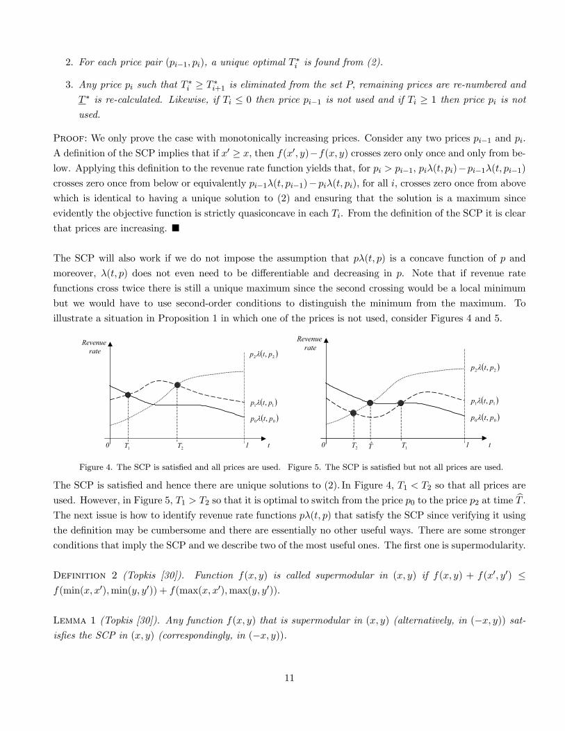
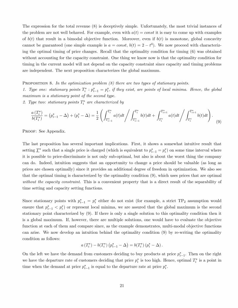
illustrate a situation in Proposition 1 in which one of the prices is not used, consider Figures 4 and 5.

t

Revenue rate

10

( )22 , ptp λ

( )00 , ptp λ

( )11 , ptp λ

1T 2T

Figure 4. The SCP is satisfied and all prices are used.

T̂ t

Revenue rate

10

( )22 , ptp λ

( )00 , ptp λ

( )11 , ptp λ

1T 2T

Figure 5. The SCP is satisfied but not all prices are used.

The SCP is satisfied and hence there are unique solutions to (2). In Figure 4, T1 < T2 so that all prices are

used. However, in Figure 5, T1 > T2 so that it is optimal to switch from the price p0 to the price p2 at time bT .The next issue is how to identify revenue rate functions pλ(t, p) that satisfy the SCP since verifying it using

the definition may be cumbersome and there are essentially no other useful ways. There are some stronger

conditions that imply the SCP and we describe two of the most useful ones. The first one is supermodularity.

Definition 2 (Topkis [30]). Function f(x, y) is called supermodular in (x, y) if f(x, y) + f(x0, y0) ≤f(min(x, x0),min(y, y0)) + f(max(x, x0),max(y, y0)).

Lemma 1 (Topkis [30]). Any function f(x, y) that is supermodular in (x, y) (alternatively, in (−x, y)) sat-isfies the SCP in (x, y) (correspondingly, in (−x, y)).

11

Supermodularity is a stronger condition than the SCP since it essentially requires that an increase in one

variable increases the incremental return to the increase of the other variable, which is a stronger no-

tion of complementarity than the SCP. Indeed, we can re-state Definition 2 as follows: for pi > pi−1,piλ(pi, t)−pi−1λ(pi−1, t) is monotonically increasing in t for all t, i.e., under the supermodularity assumptionnot only do revenue rate curves cross once but also the absolute distance between them first monotonically

decreases and then monotonically increases. Hence, supermodularity of the revenue rate function implies

concavity of the objective function. As we will see shortly, there are straightforward methods to characterize

supermodular functions, making them more convenient to work with than SCP functions. For example,

verifying that ∂2f(x, y)/∂x∂y ≥ 0 is sufficient to show supermodularity. In addition, supermodularity is

preserved under convex increasing transformations and it is also preserved under addition, which allows easy

construction and recognition of supermodular functions. A second sufficient condition for the SCP is Total

Positivity.

Definition 3 (Karlin [18]). Function f(x, y) is called totally positive of order 2 (TP2) if f(x, y) ≥ 0 and¯̄̄̄¯ f(x, y) f(x, y0)f(x0, y) f(x0, y0)

¯̄̄̄¯ ≥ 0

for all x < x0, y < y0.

Lemma 2 (Topkis [30]). Any function f(x, y) that is TP2 in (x, y) (alternatively, (−x, y)) satisfies the SCPin (x, y) (correspondingly, in (−x, y)).

Like supermodularity, TP2 is stronger than the SCP. To see this, re-state Definition 3 as follows: for

pi > pi−1, piλ(pi, t)/pi−1λ(pi−1, t) is monotonically increasing in t for all t. This statement directly impliesthat piλ(pi, t)/pi−1λ(pi−1, t) crosses 1 only once, which ensures that the SCP holds. Unlike supermodularityand similar to the SCP, TP2 does not require monotonicity of the absolute distance between the two revenue

rates. Hence, generally speaking TP2 is neither implied by nor does it necessarily imply supermodularity.

Note that, similar to the SCP property, TP2 ensures strict quasi-concavity of the objective function. TP2 is

preserved under multiplication which, again, allows the construction of TP2 functions with ease. It is now

desirable to obtain conditions for the demand function λ(t, p) that guarantee the SCP for the revenue rate

function pλ(t, p). We will state several related results.

Proposition 2. If any of the following is true about λ(t, p) (or λ(t,−p)):1. λt(t, p) + pλtp(t, p) ≥ 0, ∀t, p;2. λ(t, p)λtp(t, p)− λt(t, p)λp(t, p) ≥ 0, ∀t, p;3. λt(t,p)

λ(t,p) is non-decreasing in p, ∀t;4.

λp(t,p)λ(t,p) is non-decreasing in t, ∀p;

5. λ(t,p0)λ(t,p) is non-decreasing in t for p

0 ≥ p;6. λ(t0,p)

λ(t,p) is non-decreasing in p for t0 ≥ t;

12

then the revenue rate function pλ(t, p) satisfies the SCP in (p, t) (correspondingly, in (−p, t)).Proof: See Appendix.

This set of conditions can be readily applied to any functional form of λ(t, p) and some of these conditions

have intuitive interpretations that enhance managerial intuition. For example, consider Condition 3. Define

the time-elasticity of demand at time t when price is p as follows:

²t(t, p) =∂λ(t, p)/ ∂t

λ(t, p)/ t,

which gives the relative rate of change (or the speed of change) in the demand with time. This way con-

dition 3 has an intuitive interpretation. For example, to ensure that pi−1 < pi (the airline case), we wouldrequire that at any point the time-elasticity of the demand is increasing in price and in case pi−1 > pi

(retailing), we would want the time-elasticity to decrease in price. It also helps to focus on a very specific

case: for instance, ²t(t, pi) < 0 (demand is decreasing with time at price pi). Then the proposition says

that, for pi−1 < pi to be optimal, it is sufficient for the demand to be decreasing at price pi−1 as well andmoreover, at price pi−1 the demand should decline more quickly (i.e., the absolute speed of change is higher).

In economics, demand elasticity typically refers to price-elasticity of demand, i.e., change in demand relative

to change in price. Condition 4 is convenient in that it can be interpreted in terms of the price-elasticity of

demand. Indeed, define the price-elasticity of demand at time t and price p as follows:

²p(t, p) =∂λ(t, p)/ ∂p

λ(t, p)/ p.

Then Condition 4 requires that the price-elasticity of demand be non-decreasing over time. The time-

elasticity defined above is quite different from price-elasticity: the former can be positive as well as negative

and the latter is typically negative. In most cases, price-elasticity is defined in terms of absolute value so that

higher price-elasticity is associated with lower optimal price and vice versa. The following three examples

demonstrate applications of other conditions of Proposition 2.

Example 1: λ(t, p) = a− tp satisfies Condition 1 in (−p, t) because

λt(t, p) + pλtp(t, p) = −2p ≤ 0.

Example 2: λ(t, p) = a(t)− p2 satisfies Condition 2 in (p, t) for increasing a(t) because

λ(t, p)λtp(t, p)− λt(t, p)λp(t, p) = 2pa0(t) ≥ 0.

Example 3: λ(t, p) = a(t)e−p/b(t) satisfies Condition 5 if b(t) is increasing in t because

λ(t, p0)λ(t, p)

= e(p−p0)/b(t),

is non-decreasing in t. Note also that the application of Conditions 1 and 2 in this case is not prudent since

taking derivatives is quite cumbersome. It is worth pointing out here that Feng and Gallego [13] use TP2

13

property to demonstrate monotonicity results in a setting with pre-determined prices and time-invariant

Poisson arrivals. However, since TP2 naturally holds for the Poisson arrival process, they do not generalize

this result to other arrival processes. Later, Feng and Gallego [14] state that it is difficult to derive similar

conditions if the time-invariance assumption is relaxed. In this sense, our monotonicity results are more

general and one can hope that they also hold in a more realistic stochastic setting.

Since prices are given exogenously, it is important to understand the impact that an increase or decrease

in price (possibly due to a change in the competitive market situation) has on the optimal timing of price

changes. For this purpose the SCP provides the necessary and sufficient condition for monotone comparative

statics since it ensures complementarity between p and t, meaning that any increase/decrease in price will

increase/decrease the optimal time to change prices.

Lemma 3 (Milgrom and Shannon [25]). Let X be a lattice, S ⊂ X, Y a partially ordered set, and

f(x, y) : X × Y → R. Then argmaxx∈S f(x, y) is monotone non-decreasing in (y, S) if and only if f(x, y)is quasisupermodular in x and satisfies the SCP in (x, y).

Unfortunately, the fact that the revenue rate function satisfies the SCP does not necessarily imply that the

objective function satisfies it as well. Moreover, the sufficient condition for the objective function to satisfy

the SCP appears cumbersome. Instead, we use a stronger notion of supermodularity to obtain the desired

result.

Proposition 3. Define bp(t) = argmaxp pλ(t, p) and suppose that the revenue rate function satisfies the SCPin (p, t). Then the optimal solution T ∗i is increasing in pi if pi > bp(T ∗i ) and is decreasing in pi if pi < bp(T ∗i ).Correspondingly, T ∗i is decreasing in pi−1 if pi−1 > bp(T ∗i ) and is increasing in pi−1 if pi−1 < bp(T ∗i ).Proof: We prove the statement for pi only. Notice that, once Proposition 1 is applied, the problem is

separable in all T ∗i . Supermodularity of the objective function in (Ti, pi) implies the SCP in (Ti, pi) andhence is sufficient for T ∗i to be monotone increasing in pi (see Lemma 3). To verify supermodularity, it issufficient to ensure that the second-order cross-partial derivative is non-negative:

∂2π

∂Ti∂pi= − ∂

∂pi(piλ(Ti, pi)) .

Notice that the expression in brackets is the revenue rate function, which is assumed to be concave. From

the definition of bp(t) it follows that the revenue rate function is decreasing at any pi > bp(T ∗i ), i.e.,∂2π

∂Ti∂pi= − ∂

∂pi(piλ(Ti, pi)) > 0, ∀pi > bp(Ti)

so that the objective function is supermodular and T ∗i is increasing in pi (see Lemma 3). Otherwise,

∂2π

∂Ti∂pi= − ∂

∂pi(piλ(Ti, pi)) < 0, ∀pi < bp(Ti)

14

and the objective function is submodular so that T ∗i is decreasing in pi.¥

The last result is important in understanding the implications that competitive and other forces affecting

prices might have on the timing of price changes and shows that such effect is non-trivial since increase in

price can lead to either increase or decrease in the timing of price change. To develop the intuition, lets

focus on monotonicity of T ∗i w.r.t. pi. To see why T∗i is decreasing in pi on pi ∈ [0, bp(T ∗i )) and is increasing

on pi ∈ (bp(T ∗i ),∞), observe that on the former interval∂2π

∂Ti∂pi= −λ(Ti, pi)− piλp(Ti, pi) < 0,

or equivalently |²p(t, p)| < 1, while on the latter interval |²p(t, p)| > 1. It is conventional to say in the formercase that demand is inelastic (since a unit-increase in price decreases the demand by less than a unit) and in

the latter case that demand is elastic. Hence, if at some price demand is inelastic, an increase in pi naturally

makes it more profitable to charge pi on a longer time interval because the price increase outweighs the

demand decrease and leads to an increase in the revenue rate. Since revenue rate is concave in p, revenues

are decreasing (demand is elastic) for any p > bp and revenues are increasing (demand is inelastic) for anyp < bp.The analysis of the optimal timing decision so far has been done without the capacity constraint. We shall

now turn to the problem in which, in addition to timing, the capacity may be set optimally

maxπ = maxC

maxT0≤T1≤...≤TN+1

PNi=0

R Ti+1Ti

piλ(t, pi)dt

s.t. p ∈ P, PNi=0

R Ti+1Ti

λ(t, pi)dt ≤ C

−K2(C) .

It turns out that the complementarity between p and t in the form of TP2 condition imposed on the revenue

rate function is sufficient to guarantee uniqueness of the solution. Moreover, optimal timing of price changes

is monotone in the capacity constraint.

Proposition 4. Suppose that the revenue rate function pλ(p, t) is TP2 in (p, t) (alternatively, in (−p, t)).Then:

1. Prices are non-decreasing (non-increasing), p0 ≤ p1 ≤ ... ≤ pN .

2. There is a unique T ∗ characterized by the following optimality conditions

(pi−1 − µ)λ(Ti, pi−1)− (pi − µ)λ(Ti, pi) = 0, i = 1, ...,N,

where Lagrange multiplier µ = 0 if capacity is not a constraint and µ is found from the capacity

constraint otherwise.

3. All T ∗i s are non-decreasing (non-increasing) in C.

4. The objective function π(C) is concave in C and hence there is a unique solution to the capacity

problem.

15

Proof: See Appendix.

Results 1, 2 and 4 are direct extensions of Proposition 1 to the capacitated problem while result 3 is new.

The intuition behind monotonicity of all T ∗i s in capacity is as follows: lower capacity should lead to higheraverage price. However, since prices are exogenously given, higher average price can only be achieved through

charging higher prices on longer time intervals. Hence, for example, we increase the average price by short-

ening time interval [T0, T1] where the lowest price p0 is charged and widening time interval [TN , TN+1] where

the highest price pN is charged. It is, however, not immediately clear if any other time interval extends or

shortens although all intervals do shift to the left. Result 4 is rather standard and appeared (under different

assumptions) in Gallego and van Ryzin [16], and in Zhao and Zheng [33].

Note that, although uniqueness and the structure of the solution are preserved under the capacity constraint,

monotonicity of timing w.r.t. price (Proposition 3) appears difficult to prove. The reason is that the

application of monotonicity properties like the SCP, supermodularity and TP2 requires that the decision

space be a lattice (see Lemma 3), but with the capacity constraint it is no longer obvious that the decision

space is a lattice and the analysis breaks down. To summarize, we have seen that, when prices are exogenously

given, finding the optimal timing of a limited number of price changes is significantly harder than when

the number of such changes is not limited. Nevertheless, we were able to find conditions that guarantee

uniqueness of the solution (otherwise the problem is not well-behaved in the sense that multiple local minima

and maxima are possible) and characterize situations in which prices are monotone throughout the sales

period. For a non-capacitated problem we also describe the effects of exogenous price changes on the timing

of these changes. We now turn to the problem with endogenized pricing decision.

4.2 Endogenous prices

Just as we did previously, we consider the simplified problem with pre-determined timing of price changes

first. One example of the situation in which timing is pre-determined is retail sales events tied to major

holidays or the weather. This setting has received some attention in the literature (see Bitran and Mondschein

[5]). Further, for the time being ignore the capacity constraint. The optimization is

maxπ = maxp

"NXi=0

Z Ti+1

Ti

piλ(t, pi)dt

#. (3)

This problem is separable in decision variables so one has to solve N + 1 pricing problems with a single

price each (i.e., the non-discriminating case) and the solution is trivially unique due to the concavity as-

sumption about the revenue rate function. An interesting question in this setting is the characterization of

the impact that the timing has on prices; i.e., if for some reason there is a need to adjust timing, what is

the corresponding change in prices? Such a situation may occur if, for example, the company would like to

test the sensitivity of prices to external factors (e.g., weather) that may force changes in the timing of price

changes and hence changes in pricing. To answer this question we employ methodology similar to that in

Proposition 3, only this time T is a parameter and p is a decision variable.

16

Proposition 5. Define bp(t) = argmaxp pλ(t, p). Then the optimal solution p∗i−1 (Ti−1, Ti) is increasing inTi if p

∗i−1 (Ti−1, Ti) < bp (Ti) and is decreasing in Ti if p∗i−1 (Ti−1, Ti) > bp (Ti) . Correspondingly, the optimal

solution p∗i (Ti, Ti+1) is decreasing in Ti if p∗i (Ti, Ti+1) < bp (Ti) and is increasing in p∗i if p∗i (Ti, Ti+1) > bp (Ti) .

Proof: Follows along the lines of the Proof of Proposition 3. ¥

Proposition 5 shows that complementarity between p and t helps characterize situations in which prices are

monotone in timing, thus complementing Proposition 3. The similarity between the results of Propositions 3

and 5 is due to the symmetry of the supermodularity property: i.e., a function f(x, y) that is supermodular

in (x, y) is also supermodular in (y, x) (this is not necessarily the case for the SCP). As in Proposition 3,

the intuition behind the result can be gained by considering demand elasticity. We now turn to the more

general problem with the capacity constraint but still keep timing exogenous:

maxπ = maxC

"maxp

PNi=0

R Ti+1Ti

piλ(t, pi)dt

s.t.PNi=0

R Ti+1Ti

λ(t, pi)dt ≤ C−K2(C)

#. (4)

Pricing problems on each time interval are no longer separable; all prices are linked through the capacity

constraint. We saw that, when there is only one price, a tighter capacity constraint increases the price. The

natural question is: does this result hold when there are several prices charged throughout the selling period

or will some prices rise while others fall? The next proposition assures that all prices are decreasing in the

capacity constraint and moreover, there is a unique optimal capacity.

Proposition 6.

1. The objective function (4) is jointly concave in p and unique optimal prices are characterized by the

following optimality conditions

p∗i (Ti, Ti+1) = −R Ti+1Ti

λ(t, p∗i )dtR Ti+1Ti

λp(t, p∗i )dt+ µ, i = 0, ..., N, (5)

where Lagrange multiplier µ = 0 if capacity is not a constraint and µ is found from the capacity

constraint otherwise.

2. All p∗i s are non-increasing in C.

3. The objective function (4) is concave in C so that there is a unique solution C∗ to the capacity problem.

Proof: See Appendix.

The second result of Proposition 6 can be paralleled with the result in Federgruen and Heching [12] and other

papers so that, in a simultaneous pricing/inventory replenishment problem, the optimal price is decreasing in

the amount of initial inventory. However, because multiple prices are involved in our problem, the technique

for showing this result is different: as was mentioned earlier, the supermodularity argument cannot be applied

here the same way as in Federgruen and Heching [12] because the decision space is not a lattice. Results 2

17

and 3 also appeared (under different assumptions) in Gallego and van Ryzin [16], and in Zhao and Zheng [33].

The solution to the problem with exogenous prices is useful by itself but it also helps us characterize a

solution to the more general problem of jointly finding optimal pricing, timing, and capacity:

maxπ = maxC

"max

T0≤T1≤...≤TN+1

"maxp

PNi=0

R Ti+1Ti

piλ(t, pi)dt

s.t.PNi=0

R Ti+1Ti

λ(t, pi)dt ≤ C

#−K2(C)

#.

Optimal pricing solution p∗(T ) can be borrowed from Proposition 6, so we proceed with obtaining optimal

timing when prices are chosen optimally. The first derivatives are found as follows:

∂π

∂Ti=

∂p∗i−1∂Ti

ÃZ Ti

Ti−1λ(t, p∗i−1)dt+ p

∗i−1

Z Ti

Ti−1λp(t, p

∗i−1)dt

!+ p∗i−1λ(Ti, p

∗i−1)

+∂p∗i∂Ti

µZ Ti+1

Ti

λ(t, p∗i )dt+ p∗i

Z Ti+1

Ti

λp(t, p∗i )dt

¶− p∗iλ(Ti, p∗i ), i = 1, ...,N.

When the capacity constraint is binding, there is no easy way to simplify (6), so the optimality condition

remains quite intractable. However, if capacity is specified exogenously and the constraint is not binding (or

if capacity is ample), then µ = 0 and we can make use of the fact that prices are chosen optimally according

to (5): the expressions in brackets vanish and the first-order necessary conditions for optimal timing are

characterized by

p∗i−1(T∗i−1, T

∗i )λ(T

∗i , p

∗i−1(T

∗i−1, T

∗i )) = p

∗i (T

∗i , T

∗i+1)λ(T

∗i , p

∗i (T

∗i , T

∗i+1)), i = 1, ..., N. (6)

We see that the optimality conditions are essentially the same as when prices are exogenously given and

hence the interpretation is similar: whenever instantaneous revenue rates from two prices are equal, there is

a stationary point. The difference is, of course, that this time prices are functions of T . As will be demon-

strated later, without restrictions on λ(t, p) the objective function can easily be multimodal in T with many

local maxima and minima. However, this complication does not preclude us from establishing a sufficient

condition for price monotonicity throughout the sales period, which is important for developing simple pric-

ing rules in practice.

Proposition 7. Suppose the revenue rate function is TP2 in (t, p) (correspondingly, in (−t, p)). Then theoptimal pricing policy is monotonically increasing (correspondingly, decreasing) throughout the sales period

for any T , C, and N .

Proof: See Appendix.

The last result provides a rather simple tool for identifying situations in which prices are monotone through-

out the selling period. We see once again that complementarity (in the form of TP2) between price and time

can be instrumental in characterizing the optimal pricing policy. The important take away from the last

proposition can be verbalized through price elasticity of demand: using characterization 4 in Propositions

2 we can say that increasing (decreasing) price elasticity implies increasing (decreasing) prices. Recall that

higher price elasticity is a necessary and sufficient condition for a higher optimal price in a static monopoly

18

pricing model and furthermore, it is possible to verify that the condition of Proposition 7 is necessary and

sufficient for continuous dynamic price p∗(t) to be monotone (Zhao and Zheng [34] demonstrate a relatedresult in a stochastic setting). We have shown that the same condition is sufficient (but clearly not necessary)

for the pricing policy with a limited number of price adjustments to be monotone.

We close this section with the analysis of a specific form of the demand function. Suppose that the demand

function is multiplicatively separable in t and p, i.e., λ(t, p) = α(t)β(p). This form of the demand function

has been popular in the literature due to its analytical convenience (see Gallego and van Ryzin [16], Feng

and Gallego [13], and Gallego [15]). Using (5), we can find optimal prices as follows:

p∗i = −β(p∗i )

R Ti+1Ti

α(t)dt

βp(p∗i )R Ti+1Ti

α(t)dt+ µ = − β(p∗i )

βp(p∗i )+ µ, i = 0, ..., N.

Clearly, all prices are equal, which is the equivalent of not price discriminating. Hence, in the absence

of demand uncertainty there is no benefit in charging multiple prices when such functional form is used.

This result extends the finding of Gallego and van Ryzin [16] that charging a single price is optimal in the

continuous version of the problem. Intuitively, this result is a consequence of the fact that ²p = const for

this form of demand function.

5 Linear pricing model

To gain further insights into the problem, for the remainder of the paper we introduce simplifying assumptions

regarding the demand function λ(p, t). Specifically, we use the following model of customer behavior. Suppose

that at any point of time t customers considering the purchase arrive at a rate a(t) and find out that the

current price is p. At this point b(t)p customers decide that the price is too high, leave and never return.

The remaining a(t) − b(t)p customers decide to make a purchase. Hence, from the company’s point of

view, purchasing customers arrive continuously at a rate λ(p, t) = a(t)− b(t)p. An equivalent interpretationis: a(t) is the customer arrival rate and the purchase is made with probability 1 − b(t)p/ a(t). This formof the demand function is used frequently in the marketing literature (see an extensive discussion of this

assumption and additional references in Eliashberg and Steinberg [10]; our demand model is slightly more

general since we allow that not only a(t) but also b(t) is a function of time). Functions a(t) and b(t) can

be interpreted as demand intensity and price sensitivity, correspondingly. We assume that both a(t) and

b(t) are positive differentiable functions. Essentially, we assume that customer demand is linear in price but

non-linear in time, and the effects of time-varying market size and price-sensitivity are separated, making the

model intuitively appealing (as noted by Eliashberg and Steinberg [10]). We also assume that the problem

parameters are such that it is never optimal to charge a price higher than a(t)/b(t) (i.e., at any point of

time there is a non-zero demand). Assumptions similar to this one are standard in the marketing literature

that uses the same demand function (for example, it is conventional to assume that p(t) ≤ a(t)/b(t) as inEliashberg and Steinberg [10] and citations therein). We will proceed by solving the problem backwards and

analyzing pricing, timing, and capacity choices separately.

19

5.1 Price optimization

Suppose for now that C and T are exogenously given and focus on pricing. Using the result of Proposition

6, for a given arbitrary C and T optimal prices can be found in a closed form as follows:

p∗i (Ti, Ti+1, C) =Z Ti+1

Ti

a(t)dt

Áµ2

Z Ti+1

Ti

b(t)dt

¶+∆, ∀i, (7)

where ∆ = max³0,R 10 a(t)dt− 2C

´.³2R 10 b(t)dt

´. Observe at this point that the impact of the increase

in the capacity constraint is quite intuitive: if T is fixed, prices will decrease, and moreover, an increase in

capacity results in the increase of all prices by the same amount so that the price differential between any

two prices remains constant. Further, the condition of Proposition 7 (price monotonicity) can be simply

re-stated as follows: if a(t)/b(t) is monotonically increasing (decreasing) in t, then prices are monotonically

increasing (decreasing) throughout the sales period. To gain some intuition, it helps to think about ratio

a(t)/ b(t) as “customer density” per unit of demand sensitivity. If customer density is increasing with time,

price is rising and vice versa.

5.2 Optimization of timing

We now turn to optimization over T . First, we use optimal prices to re-write the objective function as

follows:

π =NXi=0

õZ Ti+1

Ti

a(t)dt

¶2,µ4

Z Ti+1

Ti

b(t)dt

¶!−∆2

Z 1

0b(t)dt−K2(C). (8)

The first term represents optimal revenue in the absence of the capacity constraint (it only depends on the

timing and the number of price changes). The last two terms represent capacity cost that does not depend

on optimal timing. What is important is that we can separate timing decision and optimal capacity choice,

meaning that the capacity choice decision does not affect the timing of price changes, and vice versa. This

unexpected result greatly simplifies further derivations and it also has important implications for compa-

nies operating in the environments that can be characterized by the model discussed in this section (i.e.,

the model with linear pricing). For example, if companies with different capacities (product inventories)

face the same market conditions (i.e., the same demand function) then they will establish the same timing

of price changes (even though prices will be different). Since timing and capacity decisions are separable,

the marketing function of setting the timing of price changes (e.g., promotions) can be separated from the

operational function of making capacity decisions as long as prices are coordinated with operations. This is

an important implication since capacity decisions often have to be made far in advance but it is possible to

postpone pricing and timing decisions. Moreover, the form of price discrimination (i.e., the number of price

changes) does not need to be decided at the time of capacity choice since it affects revenues but not costs.

Finally, we can conclude that an increase in capacity will lead to a decrease in all prices by the same amount

without the stipulation that T should be kept constant (as was observed in the previous subsection). The

timing problem can now be reduced from profit maximization to revenue maximization (the first term in 8).

20

The expression for the total revenue (8) is deceptively simple. Unfortunately, the most trivial instances of

the problem are not well behaved. For example, even with a(t) = const it is easy to come up with examples

of b(t) that result in a bimodal objective function. Moreover, even if b(t) is monotone, global concavity

cannot be guaranteed (one simple example is a = const, b(t) = 2 − t4). We now proceed with characteriz-ing the optimal timing of price changes. Recall that the optimality condition for timing (6) was obtained

without accounting for the capacity constraint. One thing we know now is that the optimality condition for

timing in the current model will not depend on the capacity constraint since capacity and timing problems

are independent. The next proposition characterizes the global maximum.

Proposition 8. In the optimization problem (8) there are two types of stationary points.

1. Type one: stationary points T ∗i : p∗i−1 = p∗i , if they exist, are points of local minima. Hence, the global

maximum is a stationary point of the second type.

2. Type two: stationary points T ∗i are characterized by

a (T ∗i )b(T ∗i )

=¡p∗i−1 −∆

¢+ (p∗i −∆) =

1

2

ÃZ T ∗i

T∗i−1a(t)dt

,Z T∗i

T ∗i−1b(t)dt+

Z T∗i+1

T ∗ia(t)dt

,Z T ∗i+1

T ∗ib(t)dt

!.

(9)

Proof: See Appendix.

The last proposition has several important implications. First, it shows a somewhat intuitive result that

setting T ∗ such that a single price is charged (which is equivalent to p∗i−1 = p∗i ) on some time interval where

it is possible to price-discriminate is not only sub-optimal, but also is about the worst thing the company

can do. Indeed, intuition suggests that an opportunity to change a price should be valuable (as long as

prices are chosen optimally) since it provides an additional degree of freedom in optimization. We also see

that the optimal timing is characterized by the optimality condition (9), which uses prices that are optimal

without the capacity constraint. This is a convenient property that is a direct result of the separability of

time setting and capacity setting functions.

Since stationary points with p∗i−1 = p∗i either do not exist (for example, a strict TP2 assumption wouldensure that p∗i−1 < p∗i ) or represent local minima, we are assured that the global maximum is the second

stationary point characterized by (9). If there is only a single solution to this optimality condition then it

is a global maximum. If, however, there are multiple solutions, one would have to evaluate the objective

function at each of them and compare since, as the example demonstrates, multi-modal objective functions

can arise. We now develop an intuition behind the optimality condition (9) by re-writing the optimality

condition as follows:

a (T ∗i )− b(T ∗i )¡p∗i−1 −∆

¢= b(T ∗i ) (p

∗i −∆) .

On the left we have the demand from customers deciding to buy products at price p∗i−1. Then on the rightwe have the departure rate of customers deciding that price p∗i is too high. Hence, optimal T

∗i is a point in

time when the demand at price p∗i−1 is equal to the departure rate at price p∗i .

21

5.3 Setting capacity optimally

It turns out that the optimal capacity decision problem is exactly the same no matter what number of

price adjustments is used, as can be seen by considering (8). Indeed, as we have said previously, timing

and capacity decisions are separable and hence the problem of finding optimal capacity becomes that of

minimizing capacity cost (the last two terms of (8)). The optimal capacity is

C∗ =1

2

Z 1

0a(t)dt− 1

2K 02 (C

∗)Z 1

0b(t)dt,

so that if capacity is costless then K2(C) = 0 and it is optimal to purchaseR 10 a(t)dt

.2 units and sell

everything. The result that optimal capacity is independent of the type of price discrimination (for the

linear demand function) is important for companies that have to invest into the capacity far in advance,

before the pricing strategy (including type of price discrimination, number of price changes and specific

prices) is established. As we have demonstrated, such investment decisions do not have to take into account

the pricing strategy. Additionally, the administrative cost of price changes may be uncertain so that the

company may have to invest into the capacity without knowing how many price changes will be used.

5.4 Setting the number of price changes optimally

Maximization problem (8) for the optimal timing of price changes is rather involved even for the simple

forms of the arrival function. However, for illustrative purposes, we will demonstrate the optimal timing

of price changes for a couple of simple examples. Let πi denote the optimal revenue (since costs are the

same we can safely ignore them) with i price changes. Then the relative revenue loss can be calculated

as δi = 100% × (π∞ − πi) /π∞, which gives us the percentage loss due to the insufficient number of pricechanges relative to the maximum achievable revenue. Consider the following two arrival rate functions:

Case 1. a(t) = 1 + t, b(t) = 1. In this case, the price sensitivity of customers is time-invariant while the

market size is a linear increasing function of time. If price sensitivity is time-invariant, price changes are

simply spread uniformly over the time period Ti = (i − 1)/N, i = 2, ..., N (this result can be shown much

more generally).

Case 2. a(t) = 1, b(t) = 1 + t. In this case price sensitivity is not time-invariant and it can be shown

that optimal price changes are made at Ti = −1 + 2 i−1N , i = 2, ..., N. For example, one price change wouldhappen at T1 = 0.414214, two price changes would happen at T1 = 0.259921 and T2 = 0.587401, etc. That

is, there is a tendency to make price changes earlier rather than later since price sensitivity is very low at

the beginning and more profit can be extracted early in the season by administering frequent price changes.

It seems plausible that such a result should hold more generally.

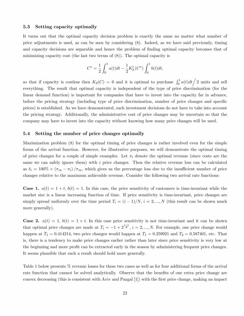
Table 1 below presents % revenue losses for these two cases as well as for four additional forms of the arrival

rate function that cannot be solved analytically. Observe that the benefits of one extra price change are

convex decreasing (this is consistent with Aviv and Pazgal [1]) with the first price change, making an impact

22

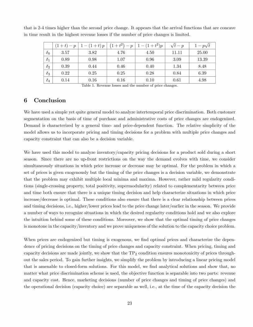
that is 2-4 times higher than the second price change. It appears that the arrival functions that are concave

in time result in the highest revenue losses if the number of price changes is limited.

(1 + t)− p 1− (1 + t) p ¡1 + t2

¢− p 1− (1 + t2)p √t− p 1− p√t

δ0 3.57 3.82 4.76 4.50 11.11 25.00

δ1 0.89 0.98 1.07 0.96 3.09 13.39

δ2 0.39 0.44 0.46 0.40 1.34 8.48

δ3 0.22 0.25 0.25 0.28 0.84 6.39

δ4 0.14 0.16 0.16 0.10 0.61 4.98Table 1. Revenue losses and the number of price changes.

6 Conclusion

We have used a simple yet quite general model to analyze intertemporal price discrimination. Both customer

segmentation on the basis of time of purchase and administrative costs of price changes are endogenized.

Demand is characterized by a general time- and price-dependent function. The relative simplicity of the

model allows us to incorporate pricing and timing decisions for a problem with multiple price changes and

capacity constraint that can also be a decision variable.

We have used this model to analyze inventory/capacity pricing decisions for a product sold during a short

season. Since there are no up-front restrictions on the way the demand evolves with time, we consider

simultaneously situations in which price increase or decrease may be optimal. For the problem in which a

set of prices is given exogenously but the timing of the price changes is a decision variable, we demonstrate

that the problem may exhibit multiple local minima and maxima. However, rather mild regularity condi-

tions (single-crossing property, total positivity, supermodularity) related to complementarity between price

and time both ensure that there is a unique timing decision and help characterize situations in which price

increase/decrease is optimal. These conditions also ensure that there is a clear relationship between prices

and timing decisions, i.e., higher/lower prices lead to the price change later/earlier in the season. We provide

a number of ways to recognize situations in which the desired regularity conditions hold and we also explore

the intuition behind some of these conditions. Moreover, we show that the optimal timing of price changes

is monotone in the capacity/inventory and we prove uniqueness of the solution to the capacity choice problem.

When prices are endogenized but timing is exogenous, we find optimal prices and characterize the depen-

dence of pricing decisions on the timing of price changes and capacity constraint. When pricing, timing and

capacity decisions are made jointly, we show that the TP2 condition ensures monotonicity of prices through-

out the sales period. To gain further insights, we simplify the problem by introducing a linear pricing model

that is amenable to closed-form solutions. For this model, we find analytical solutions and show that, no

matter what price discrimination scheme is used, the objective function is separable into two parts: revenue

and capacity cost. Hence, marketing decisions (number of price changes and timing of price changes) and

the operational decision (capacity choice) are separable as well, i.e., at the time of the capacity decision the

23

firm does not need to commit to a certain price discrimination scheme. Finally, we utilize simple examples

to illustrate the optimal timing of price changes and the impact of an additional price change.

Overall, we were able to link some notions of complementarity (single-crossing property, total positivity

and supermodularity) to monotonicity of solutions to the dynamic pricing problem and some monotone

comparative statics. While various notions of complementarity are known to lead to similar results in eco-

nomics, applications of complementarity to dynamic pricing are rare. We make precise this connection

and demonstrate methodology that might be used to derive analogous results for other problems (includ-

ing stochastic dynamic pricing). Finally, several interesting research topics can be motivated by our work.

First, an important issue that has received little attention in the literature is price discrimination under com-

petition (see Netessine and Shumsky [26] for non-price competition in revenue management): firms often

operate in an environment in which pricing decisions cannot be made in isolation from market reaction to

these decisions and hence monopoly assumption may not be satisfactory in some settings. Another issue is

incorporating consumer behavior such as gaming and diversion from one price to the other as in Gallego [15].

Our paper relies on several assumptions that limit the applicability of the results. First and foremost, we

ignore stochasticity on customer arrivals and fully focus on dynamic pricing in response to changes to shifts in

customer reservation prices. This simplification allows us to obtain cleaner technical conditions and insights.

Introducing stochasticity would require different solution techniques, see Aviv and Pazgal [1] and Xu and

Hopp [32]. One can hope that some of our results could be extendable to the stochastic demand setting;

more work is needed in this direction. The second major assumption is the absence of gaming behavior

on the consumer side. Rational consumers expect price changes and may delay/speed up their purchasing

decisions. To the best of our knowledge, Aviv and Pazgal [2] is the only dynamic pricing paper incorporating

such consumer behavior in a model with stochastic demand. This direction of research should prove fruitful

in the future.

References

[1] Aviv, Y. and A. Pazgal. 2004. A partially observed Markov decision process for dynamic pricing.

Working Paper, Washington University St. Louis.

[2] Aviv, Y. and A. Pazgal. 2003. Optimal pricing of seasonal products in the presence of forward-looking

consumers. Working Paper, Washington University St. Louis.

[3] Bertsekas, D. P. 1999. Nonlinear programming. Athena Scientific.

[4] Bitran G. and R. Caldentey. 2003. Commissioned paper: an overview of pricing models for revenue

management. Manufacturing & Service Operations Management, Vol.5, 203-229.

[5] Bitran, G. R. and S. V. Mondschein. 1997. Periodic pricing of seasonal products in retailing.Management

Science, Vol.43, 64-79.

24

[6] Brynjolfsson, E. and M. Smith. 1999. Frictionless commerce? A comparison of Internet and conventional

retailers. Management Science, Vol.46, 563-585.

[7] Bulow, J. I. 1982. Durable-goods monopolists. Journal of Political Economy, Vol.90, 314-332.

[8] Chan, L. M. A., M. Shen, D. Simchi-Levi and J. Swann. 2004. Coordinating pricing, inventory, and

production: a taxonomy and review. In Handbook Of Quantitative Supply Chain Analysis: Modeling In

The E-business Era, D. Simchi-Levi, S.D. Wu and Z.-J. Shen, editors, Kluwer.

[9] Coase, R. H. 1972. Durability and monopoly. Journal of Law and Economics, Vol.15, 143-159.

[10] Eliashberg, J. and R. Steinberg. 1987. Marketing-production decisions in an industrial channel of dis-

tribution. Management Science, Vol.33, 981-1000.

[11] Elmaghraby, W. and P. Kesinocak. 2003. Dynamic pricing in the presence of inventory considerations:

research overview, current practices, and future directions. Management Science, Vol.49, 1287-1309.

[12] Federgruen, A. and A. Heching. 1999. Combined pricing and inventory control under uncertainty. Op-

erations Research, Vol.47, 454-475.

[13] Feng, Y. and G. Gallego. 1995. Optimal starting times for end-of-season sales and optimal stopping

times for promotional fares. Management Science, Vol.46, 1371-1391.

[14] Feng, Y. and G. Gallego. 2000. Perishable asset revenue management with Markovian time dependent

demand intensities. Management Science, Vol.46, 941-956.

[15] Gallego, G. 1996. A demand model for yield management. Technical report, Columbia University.

[16] Gallego, G. and G. van Ryzin. 1994. Optimal dynamic pricing of inventories with stochastic demand

over finite horizons. Management Science, Vol.40, 999-1020.

[17] Gupta, D., A.V. Hill and T. Bouzdine-Chameeva. 2002. A pricing model for clearing end of season retail

inventory. Working Paper, University of Minnesota.

[18] Karlin, S. 1968. Total positivity. Stanford University Press.

[19] Kunreuther, H. and L. Schrage. 1973. Joint pricing and inventory decisions for constant priced items.

Management Science, Vol.19, 732-738.

[20] Levi, D., M. Bergen, S. Dutta and R. Venable. 1997. The magnitude of menu costs: direct evidence

from large US supermarket chains. Quarterly Journal of Economics, Vol.112, 791-825.

[21] Levi, D., S. Dutta, M. Bergen and R. Venable. 1998. Price adjustment at multiproduct retailers. Man-

agerial and Decision Economics, Vol.19, 81-120.

[22] Levinthal, D.A. and D. Purohit. 1989. Durable goods and product obsolescence. Marketing Science,

Vol. 8, 35-56.

25

[23] Lilien, G.L., P. Kotler and K.S. Moorthy. 1992. Marketing models. Prentice Hall.

[24] McGill, J. I., and G. van Ryzin. 1999. Revenue management: research overview and prospects. Trans-

portation Science, Vol.33, 233-256.

[25] Milgrom, P. and C. Shannon. 1994. Monotone comparative statics. Econometrica, Vol.62, 157-180.

[26] Netessine, S. and R. Shumsky. 2004. Revenue management games. Forthcoming inManagement Science,

available at http://www.netessine.com.

[27] Rajan, A., Rakesh and R. Steinberg. 1992. Dynamic pricing and ordering decisions by a monopolist.

Management Science, Vol.38, 240-262.

[28] Rao, V.R. 1993. Pricing models in marketing. In Handbooks in operations research and management

science: Marketing by J. Eliashberg and G.L. Lilien, editors. North-Holland.

[29] Smith, S.A. and D.D. Achabal. 1998. Clearance pricing and inventory policies for retail chains. Man-

agement Science, Vol.44, 285-300.

[30] Topkis, D.M. 1998. Supermodularity and complementarity. Princeton University Press.

[31] Varian, H. 1989. Price discrimination. In Handbook of industrial organization, Vol.1, R. Schmalensee

and R. Willig, editors. North-Holland.

[32] Xu, X. and W.J. Hopp. 2004. Dynamic pricing and inventory control with demand substitution: the

value of pricing flexibility. Working Paper, Northwestern University.

[33] Zbaracki, M.J., M. Ritson, D. Levy, S. Dutta and M. Bergen. 2000. The managerial and customer

dimensions of the cost of price adjustment: direct evidence from industrial markets. Working Paper,

University of Pennsylvania.

[34] Zhao, W. and Y.-S. Zheng. 2000. Optimal dynamic pricing for perishable assets with nonhomogeneous

demand. Management Science, Vol.46, 375-388.

Appendix

Proof of Proposition 2: From Topkis [30], supermodularity for differentiable functions is equivalent to

the positivity of the second-order cross-partial derivative, i.e.,

∂2 [pλ(t, p)]

∂t∂p= λt(t, p) + pλtp(t, p) ≥ 0,

and Condition 1 is verified. For Condition 2, note that TP2 property is equivalent to log-supermodularity

(see Karlin [18]), i.e.,∂2 log [pλ(t, p)]

∂t∂p=

λ(t, p)λtp(t, p)− λt(t, p)λp(t, p)

λ2(t, p)≥ 0,

26

and the result follows. To see Conditions 3 and 4, note that the definition of TP2 functions can be restated

as follows after dividing by y0 − y and taking a limit y0 → y:¯̄̄̄¯ f(x, y)

∂f(x,y)∂y

f(x0, y) ∂f(x0,y)∂y

¯̄̄̄¯ ≥ 0, for all x < x0.

If we now replace y with t and x with p, it becomes apparent that condition 3 is equivalent to the TP2

property. Reversing the variables yields Condition 4. Conditions 5 and 6 (also called the monotone likelihood

ratio property) are obtained by taking the derivative w.r.t. t

∂

∂t

λ(t, p0)λ(t, p)

=λt(t, p

0)λ(t, p)− λ(t, p0)λt(t, p)λ2(t, p)

≥ 0,

which is an equivalent of Condition 3. Condition 6 is obtained similarly. ¥

Proof of Proposition 4: We can ignore K2(C) since it does not affect any results. We first demonstrate

that the objective function is concave at any stationary point, which means that there is only one such point

that is also a global maximum. Along the way it will be clear that the prices are monotonically increasing.

Form a Lagrangian (see Bertsekas [3]) as follows:

L(T , µ) =NXi=0

Z Ti+1

Ti

piλ(t, pi)dt− µÃ

NXi=0

Z Ti+1

Ti

λ(t, pi)dt− C!, (10)

find first derivatives :

∂L

∂Ti= (pi−1 − µ)λ(Ti, pi−1)− (pi − µ)λ(Ti, pi), i = 1, ..., N,

∂L

∂µ= −

NXi=0

Z Ti+1

Ti

λ(t, pi)dt+ C,

and second derivatives:

∂2L

∂T 2i= (pi−1 − µ)λt(Ti, pi−1)− (pi − µ)λt(Ti, pi), i = 1, ..., N, (11)

∂2L

∂Ti∂µ= −λ(Ti, pi−1) + λ(Ti, pi), i = 1, ..., N. (12)

We can form the bordered Hessian as follows:

H =

¯̄̄̄¯̄̄̄¯̄̄̄¯

0 ∂2L∂T1∂µ

∂2L∂T2∂µ

... ∂2L∂TN∂µ

∂2L∂T1∂µ

∂2L∂T 21

0 ... 0

∂2L∂T2∂µ

0 ∂2L∂T 22

... 0

... ... ... ... ...∂2L

∂TN∂µ 0 0 ... ∂2L∂T 2N

¯̄̄̄¯̄̄̄¯̄̄̄¯.

We now show that the diagonal entries of the Hessian are negative at any stationary point and moreover,

the determinant of the Hessian has sign (−1)N everywhere, which is sufficient for concavity of the objective

27

function at any stationary point, implying that there is only one stationary point that is a global maximum.

To see this, equate the first derivative to zero, solve for (pi−1 − µ) and substitute the result into (11):∂2L

∂T 2i=

(pi − µ)λ(Ti, pi)λ(Ti, pi−1)

λt(Ti, pi−1)− (pi − µ)λt(Ti, pi)

= (pi − µ)λ(Ti, pi)µλt(Ti, pi−1)λ(Ti, pi−1)

− λt(Ti, pi)

λ(Ti, pi)

¶, i = 1, ..., N.

Clearly, showing that the expression in brackets is negative is sufficient for verifying that the diagonal

elements are negative. By Proposition 2, Property 3, the TP2 assumption is sufficient for the expression in

brackets to be negative as long as pi−1 < pi for all i. It immediately follows that it is optimal to have pricesmonotonically increasing. It only remains to verify that the determinant of the Hessian has a sign (−1)N .We do so by converting the Hessian into an equivalent lower-triangular matrix whose determinant can be

computed analytically. Re-write the Hessian as follows:

NYi=1

− ∂2L∂T 2i∂2L∂Ti∂µ

¯̄̄̄¯̄̄̄¯̄̄̄¯̄̄̄¯

0 ∂2L∂T1∂µ

∂2L∂T2∂µ

... ∂2L∂TN∂µ

−³

∂2L∂T1∂µ

´2Á∂2L∂T 21

− ∂2L∂T1∂µ

0 ... 0

−³

∂2L∂T2∂µ

´2Á∂2L∂T 22

0 − ∂2L∂T2∂µ

... 0

... ... ... ... ...

−³

∂2L∂T2∂µ

´2Á∂2L∂T 22

0 0 ... − ∂2L∂TN∂µ

¯̄̄̄¯̄̄̄¯̄̄̄¯̄̄̄¯,

and add lines 2 through N + 1 to the first line:

NYi=1

− ∂2L∂T 2i∂2L∂Ti∂µ

¯̄̄̄¯̄̄̄¯̄̄̄¯̄̄̄¯̄

−PNi=1

³∂2L∂Ti∂µ

´2Á∂2L∂T 2i

0 0 ... 0

−³

∂2L∂T1∂µ

´2Á∂2L∂T 21

− ∂2L∂T1∂µ

0 ... 0

−³

∂2L∂T2∂µ

´2Á∂2L∂T 22

0 − ∂2L∂T2∂µ

... 0

... ... ... ... ...

−³

∂2L∂TN∂µ

´2Á∂2L∂T2N

0 0 ... − ∂2L∂TN∂µ

¯̄̄̄¯̄̄̄¯̄̄̄¯̄̄̄¯̄.

The resulting matrix has the same determinant as the original Hessian. Moreover, this matrix is lower-

triangular and hence its determinant can be computed by multiplying diagonal elements:

|H| = (−1)NNYi=1

∂2L∂T2i∂2L∂Ti∂µ

× (−1)N NYi=1

·∂2L

∂Ti∂µ

¸× (−1)

NXi=1

"µ∂2L

∂Ti∂µ

¶2,∂2L

∂T 2i

#

= (−1)NYi=1

·∂2L

∂T 2i

¸×

NXi=1

"µ∂2L

∂Ti∂µ

¶2,∂2L

∂T 2i

#,

and the sign of the determinant is

sign |H| = (−1)× (−1)N × (−1) = (−1)N .

28

Hence there is only one stationary point that is the global maximum. To show monotonicity of T ∗ w.r.t.the capacity constraint, we apply the Implicit Function Theorem (IFT). Denote by ∇CJ the gradient-vectorof derivatives of decision variables T and µ w.r.t. C, and by ∇2CL the gradient-vector of second-order

derivatives of the Lagrangian w.r.t. C. Then the IFT can be stated as follows: for a fixed C and optimally

chosen T ,

∇CJ = −H−1 ×∇2CL.Since the Hessian is non-singular, we can multiply both sides by H and write explicitly:¯̄̄̄

¯̄̄̄¯̄̄̄¯

0 ∂2L∂T1∂µ

∂2L∂T2∂µ

... ∂2L∂TN∂µ

∂2L∂T1∂µ

∂2L∂T 21

0 ... 0

∂2L∂T2∂µ

0 ∂2L∂T22

... 0

... ... ... ... ...∂2L

∂TN∂µ 0 0 ... ∂2L∂T 2N

¯̄̄̄¯̄̄̄¯̄̄̄¯×

¯̄̄̄¯̄̄̄¯̄̄̄

∂µ∂C∂T1∂C∂T2∂C

...∂TN∂C

¯̄̄̄¯̄̄̄¯̄̄̄ = −

¯̄̄̄¯̄̄̄¯̄̄̄

∂2L∂µ∂C∂2L

∂T1∂C∂2L

∂T2∂C

...∂2L

∂TN∂C

¯̄̄̄¯̄̄̄¯̄̄̄ .

The right-hand side has a very simple structure:

∂2L

∂µ∂C= 1,

∂2L

∂Ti∂C= 0, all i,

so that the IFT yields the following system of equations:

NXi=1

∂2L

∂Ti∂µ

∂Ti∂C

= −1,

∂2L

∂Ti∂µ

∂µ

∂C+

∂2L

∂T 2i

∂Ti∂C

= 0, all i.

From the second equation we see that ∂µ/ ∂C and ∂Ti/ ∂C must have opposite signs and moreover, ∂Ti/ ∂C

has the same sign for all i. From the first equation it is clear that ∂Ti/ ∂C > 0, all i, so that ∂µ/ ∂C < 0,

which proves Statement 3. To prove Statement 4 we can use the fact that ∂µ/ ∂C < 0 to show that the

objective function is concave in C when the timing is set optimally. Recall that the Lagrange multiplier µ

is equal to the marginal value of the capacity constraint C, i.e.,

dπ(p∗(C), µ∗(C))dC

= µ(C),

(see, e.g., Bertsekas [3] for details). Taking the second derivative yields

d2π(p∗(C), µ∗(C))dC2

=∂µ(C)

∂C,

which we have shown to be negative. It follows that the objective function is concave in C and hence there

is a unique solution to the capacity problem. ¥

Proof of Proposition 6: Once again, ignore K2(C) for simplicity. To prove concavity, re-write the inner

optimization problem in (5) similar to Proposition 1:

maxπ = maxQ

" PNi=0 pi(Qi)×Qi,

s.t.PNi=0Qi ≤ C.

#

29

What we have is a concave optimization problem subject to a linear constraint that is known to be concave.

The Lagrangian in this case is identical to (10) obtained earlier. The first derivatives are

∂L

∂pi=

Z Ti+1

Ti

(λ(t, pi) + (pi − µ)λp(t, pi)) dt, i = 0, ...,N,

from which the unique optimal prices are found and the proof of Statement 1 is complete. To show mono-

tonicity of prices w.r.t. the capacity constraint, we apply once again the IFT:¯̄̄̄¯̄̄̄¯̄̄̄¯

0 ∂2L∂p0∂µ

∂2L∂p1∂µ

... 0∂2L∂p0∂µ

∂2L∂p20

0 ... 0

∂2L∂p1∂µ

0 ∂2L∂p22

... 0

... ... ... ... ...∂2L

∂pN∂µ 0 0 ... ∂2L∂p2N

¯̄̄̄¯̄̄̄¯̄̄̄¯×

¯̄̄̄¯̄̄̄¯̄̄̄

∂µ∂C∂p0∂C∂p1∂C

...∂pN∂C

¯̄̄̄¯̄̄̄¯̄̄̄ = −

¯̄̄̄¯̄̄̄¯̄̄̄

∂2L∂µ∂C∂2L

∂p0∂C∂2L

∂p1∂C

...∂2L

∂pN∂C

¯̄̄̄¯̄̄̄¯̄̄̄ .

We can find analytically all the entries of ∇2L as follows:

∂2L

∂p2i=

Z Ti+1

Ti

(2λp(t, pi) + (pi − µ)λpp(t, pi)) dt ≤ 0, i = 0, ...,N,

∂2L

∂µ2= 0,

∂2L

∂pi∂µ= −

Z Ti+1

Ti

λp(t, pi)dt ≥ 0, i = 0, ..., N.

Elements of ∇CL are the same as in Proposition 4. Using these results, we obtain from the IFT the followingsystem of simultaneous equations that is very similar to the one obtained in Proposition 6:

NXi=0

∂2L

∂pi∂µ

∂pi∂C

= −1, (13)

∂2L

∂p2i

∂pi∂C

+∂2L

∂pi∂µ

∂µ

∂C= 0, i = 0, ..., N. (14)

From (14) we see that either ∂µ/∂C ≥ 0 and ∂pi/∂C ≥ 0 all i, or ∂µ/∂C ≤ 0 and ∂pi/∂C ≤ 0 all i dueto signs of the second derivatives. However, only ∂pi/∂C ≤ 0 all i can satisfy (13) so that ∂µ/∂C ≤ 0

and ∂pi/∂C ≤ 0 all i is the only possible solution which completes proof of Statement 2. Statement 3

immediately follows similar to Proposition 4. ¥

Proof of Proposition 7: Consider two neighboring prices, p∗i−1 and p∗i . It is sufficient to show that p∗i−1 ≤p∗i for any i. First, consider the pricing optimality condition (5) that we re-write as follows: p−µ = ψ (p) . Let

p∗ be the (unique) solution to this problem. p∗ can be found graphically as an intersection of two functionsof p: the left-hand side, which is increasing linearly in p at a rate equal to 1, and the right-hand side, which

can either be decreasing in p or increasing but at a rate less than 1. Clearly, there is a unique intersection

corresponding to the solution p∗. Imagine now that function ψ (p) is replaced by a function bψ (p) such thatbψ (p) ≥ ψ (p) , all p (see Figure 6).

30

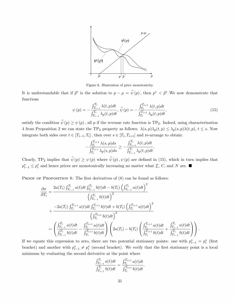
p µ

p - µ

*ˆ p *p

) ( p ψ

) ( ˆ p ψ

Figure 6. Illustration of price monotonicity.

It is understandable that if bp∗ is the solution to p − µ = bψ (p) , then p∗ < bp∗.We now demonstrate that

functions

ψ (p) = −R TiTi−1 λ(t, p)dtR TiTi−1 λp(t, p)dt

, bψ (p) = − R Ti+1Tiλ(t, p)dtR Ti+1

Tiλp(t, p)dt

, (15)

satisfy the condition bψ (p) ≥ ψ (p) , all p if the revenue rate function is TP2. Indeed, using characterization

4 from Proposition 2 we can state the TP2 property as follows: λ(s, p)λp(t, p) ≤ λp(s, p)λ(t, p), t ≤ s. Nowintegrate both sides over t ∈ [Ti−1, Ti] , then over s ∈ [Ti, Ti+1] and re-arrange to obtain:

−R Ti+1Ti

λ(s, p)dsR Ti+1Ti

λp(s, p)ds≥ −

R TiTi−1 λ(t, p)dtR TiTi−1 λp(t, p)dt

.

Clearly, TP2 implies that bψ (p) ≥ ψ (p) where bψ (p) ,ψ (p) are defined in (15), which in turn implies thatp∗i−1 ≤ p∗i and hence prices are monotonically increasing no matter what T , C, and N are. ¥

Proof of Proposition 8: The first derivatives of (8) can be found as follows:

∂π

∂Ti=2a(Ti)

R TiTi−1 a(t)dt

R TiTi−1 b(t)dt− b(Ti)

³R TiTi−1 a(t)dt

´2³R TiTi−1 b(t)dt

´2+−2a(Ti)

R Ti+1Ti

a(t)dtR Ti+1Ti

b(t)dt+ b(Ti)³R Ti+1Ti

a(t)dt´2

³R Ti+1Ti

b(t)dt´2

=

R TiTi−1 a(t)dtR TiTi−1 b(t)dt

−R Ti+1Ti

a(t)dtR Ti+1Ti

b(t)dt

2a(Ti)− b(Ti)R Ti+1Ti

a(t)dtR Ti+1Ti

b(t)dt+

R TiTi−1 a(t)dtR TiTi−1 b(t)dt

.If we equate this expression to zero, there are two potential stationary points: one with p∗i−1 = p∗i (firstbracket) and another with p∗i−1 6= p∗i (second bracket). We verify that the first stationary point is a localminimum by evaluating the second derivative at the point whereR Ti

Ti−1 a(t)dtR TiTi−1 b(t)dt

=

R Ti+1Ti

a(t)dtR Ti+1Ti

b(t)dt.

31

The second derivative is:

∂2

∂T 2i

NXi=0

³R Ti+1Ti

a(t)dt´2

R Ti+1Ti

b(t)dt

=

2a(Ti)− b(Ti)R Ti+1Ti

a(t)dtR Ti+1Ti

b(t)dt+

R TiTi−1 a(t)dtR TiTi−1 b(t)dt

∂

∂Ti

R TiTi−1 a(t)dtR TiTi−1 b(t)dt

−R Ti+1Ti

a(t)dtR Ti+1Ti

b(t)dt

=

2a(Ti)− 2b(Ti)R TiTi−1 a(t)dtR TiTi−1 b(t)dt

× 1R Ti

Ti−1 b(t)dt

a(Ti)− b(Ti)R TiTi−1 a(t)dtR TiTi−1 b(t)dt

+ 1R Ti+1Ti

b(t)dt

Ãa(Ti)− b(Ti)

R Ti+1Ti

a(t)dtR Ti+1Ti

b(t)dt

!= 2

a(Ti)− b(Ti)R TiTi−1 a(t)dtR TiTi−1 b(t)dt

× 1R Ti

Ti−1 b(t)dt

a(Ti)− b(Ti)R TiTi−1 a(t)dtR TiTi−1 b(t)dt

+ 1R Ti+1Ti

b(t)dt

a(Ti)− b(Ti)R TiTi−1 a(t)dtR TiTi−1 b(t)dt

= 2

a(Ti)− b(Ti)R TiTi−1 a(t)dtR TiTi−1 b(t)dt

2 1R TiTi−1 b(t)dt

+1R Ti+1

Tib(t)dt

> 0,

showing that at p∗i−1 = p∗i the objective function is locally convex. This completes the proof. ¥

32