Embed Size (px)
Citation preview
Dynamic-Programming Strategies for Analyzing Biomolecular Sequences

2
Dynamic Programming
• Dynamic programming is a class of solution methods for solving sequential decision problems with a compositional cost structure.
• Richard Bellman was one of the principal founders of this approach.
3
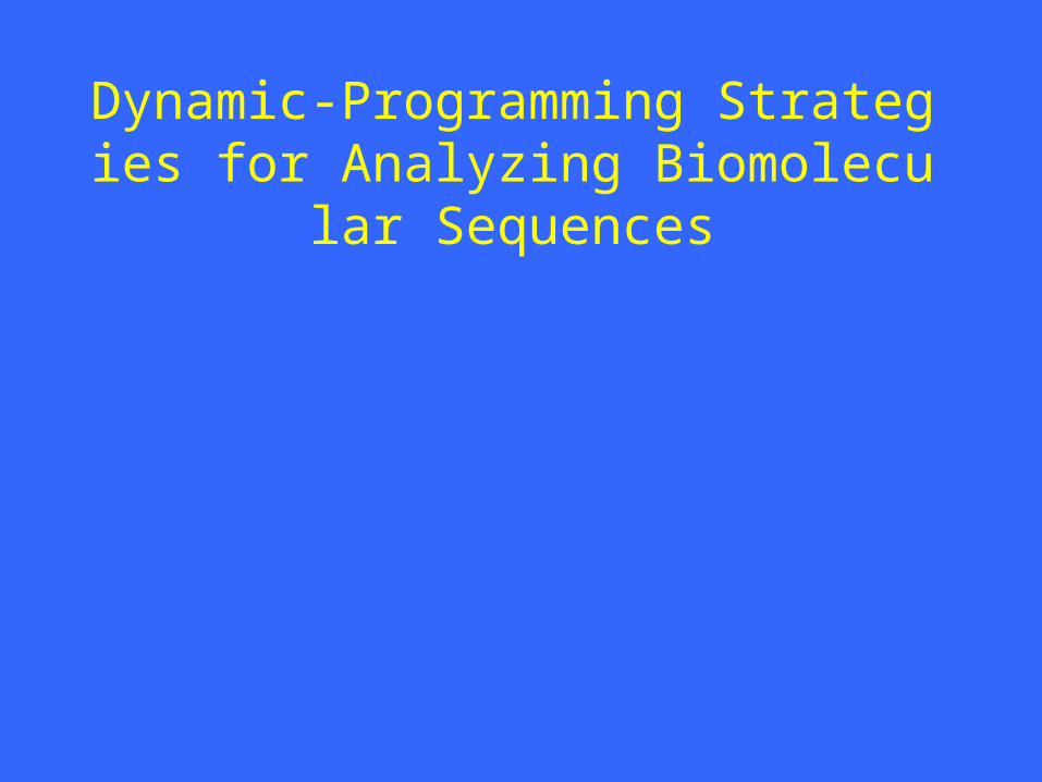
Two key ingredients
• Two key ingredients for an optimization problem to be suitable for a dynamic-programming solution:
Each substructure is optimal.
(Principle of optimality)
1. optimal substructures 2. overlapping subproblems
Subproblems are dependent.
(otherwise, a divide-and-conquer approach is the choice.)
4
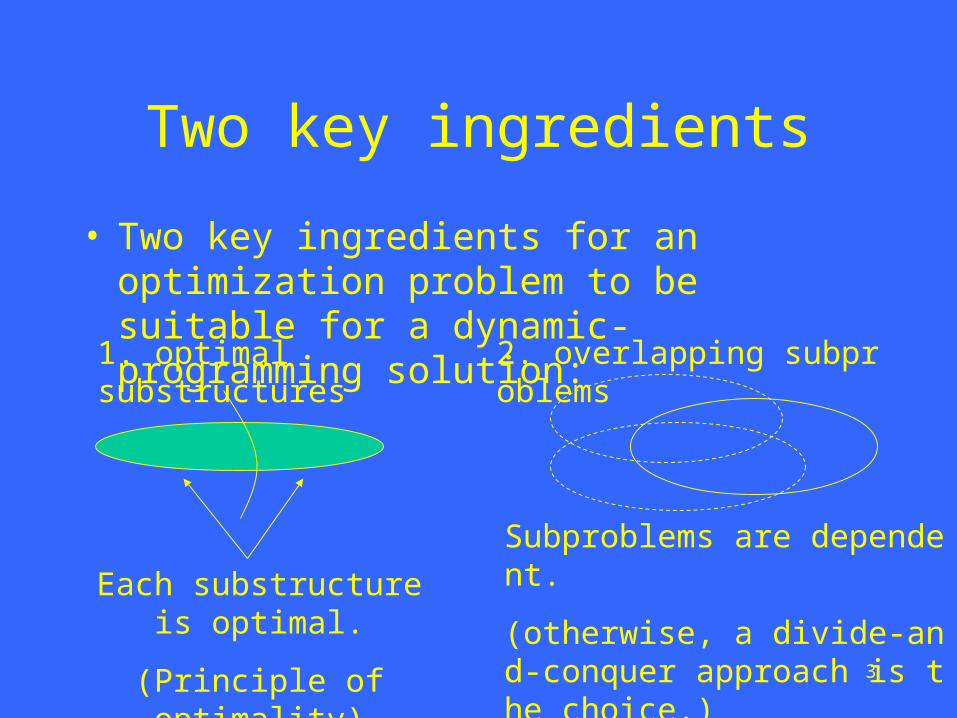
Three basic components
• The development of a dynamic-programming algorithm has three basic components:– The recurrence relation (for defining the value of a
n optimal solution);– The tabular computation (for computing the value
of an optimal solution);– The traceback (for delivering an optimal solution).
5
Fibonacci numbers
.for
21
11
00
i>1i
Fi
FiF
F
F
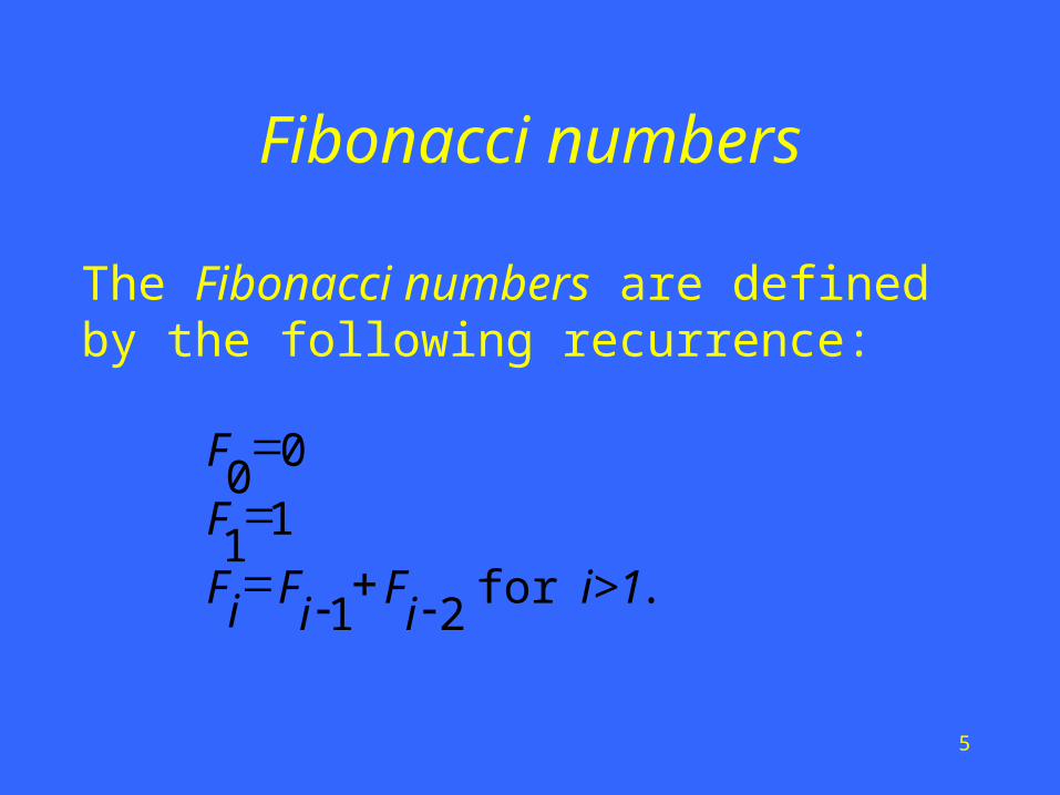
The Fibonacci numbers are defined by the following recurrence:

6
How to compute F10?
F10
F9
F8
F8
F7
F7
F6
……

7
Tabular computation
• The tabular computation can avoid recompuation.
F0 F1 F2 F3 F4 F5 F6 F7 F8 F9 F10
0 1 1 2 3 5 8 13 21 34 55

8
Maximum-sum interval
• Given a sequence of real numbers a1a2…an , find a consecutive subsequence with the maximum sum.
9 –3 1 7 –15 2 3 –4 2 –7 6 –2 8 4 -9
For each position, we can compute the maximum-sum interval starting at that position in O(n) time. Therefore, a naive algorithm runs in O(n2) time.

9
O-notation: an asymptotic upper bound
• f(n) = O(g(n)) iff there exist two positive constant c and n0 such that 0 f(n) cg(n) for all n n0
cg(n)
f(n)
n0

10
How functions grow?
30n 92n log n 26n2 0.68n3 2n
1000.003
sec.0.003 sec.
0.0026 sec.
0.68 sec.4 x 1016
yr.
100,000 3.0 sec. 2.6 min. 3.0 days 22 yr.
For large data sets, algorithms with a complexity greater than O(n log n) are often impractical!
n
function
(Assume one million operations per second.)
11
Maximum-sum interval(The recurrence relation)
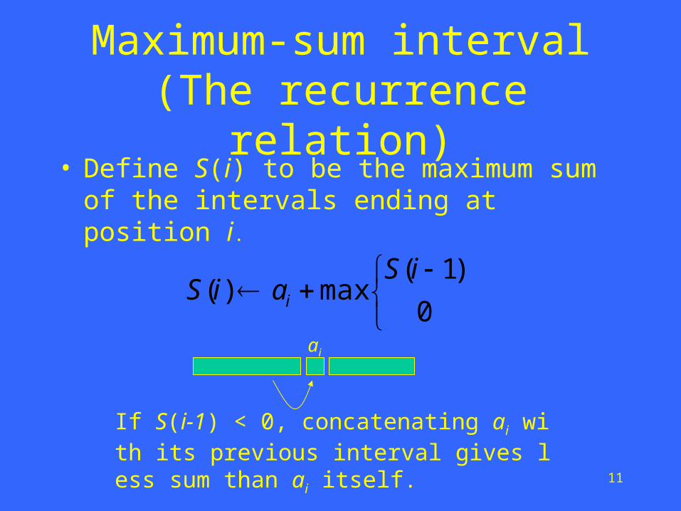
• Define S(i) to be the maximum sum of the intervals ending at position i.
0
)1(max)(
iSaiS i
ai
If S(i-1) < 0, concatenating ai with its previous interval gives less sum than ai itself.

12
Maximum-sum interval(Tabular computation)
9 –3 1 7 –15 2 3 –4 2 –7 6 –2 8 4 -9
S(i) 9 6 7 14 –1 2 5 1 3 –4 6 4 12 16 7
The maximum sum

13
Maximum-sum interval(Traceback)
9 –3 1 7 –15 2 3 –4 2 –7 6 –2 8 4 -9
S(i) 9 6 7 14 –1 2 5 1 3 –4 6 4 12 16 7
The maximum-sum interval: 6 -2 8 4

14
Longest increasing subsequence(LIS)
• The longest increasing subsequence is to find a longest increasing subsequence of a given sequence of distinct integers a1a2…an .
e.g. 9 2 5 3 7 11 8 10 13 6
2 3 7
5 7 10 13
9 7 11
3 5 11 13
are increasing subsequences.
are not increasing subsequences.
We want to find a longest one.

15
A naive approach for LIS• Let L[i] be the length of a longest increasing
subsequence ending at position i.
L[i] = 1 + max j = 0..i-1{L[j] | aj < ai}(use a dummy a0 = minimum, and L[0]=0)
9 2 5 3 7 11 8 10 13 6L[i] 1 1 2 2 3 4 ?

16
A naive approach for LIS
9 2 5 3 7 11 8 10 13 6L[i] 1 1 2 2 3 4 4 5 6 3
L[i] = 1 + max j = 0..i-1 {L[j] | aj < ai}
The maximum length
The subsequence 2, 3, 7, 8, 10, 13 is a longest increasing subsequence.
This method runs in O(n2) time.

17
Binary search
• Given an ordered sequence x1x2 ... xn, where x1<x2< ... <xn, and a number y, a binary search finds the largest xi such that xi< y in O(log n) time.
n...
n/2n/4
18
Binary search
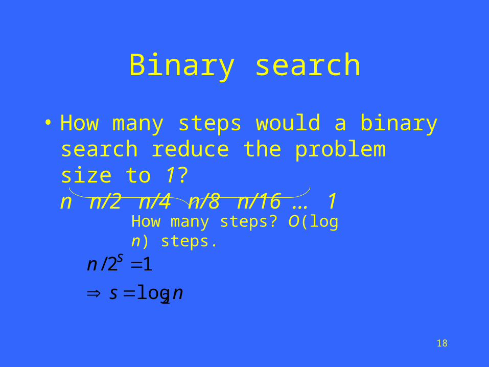
• How many steps would a binary search reduce the problem size to 1?n n/2 n/4 n/8 n/16 ... 1
How many steps? O(log n) steps.
ns
n s
2log
12/

19
An O(n log n) method for LIS
• Define BestEnd[k] to be the smallest number of an increasing subsequence of length k.
9 2 5 3 7 11 8 10 13 69 2 2
5
2
3
2
3
7
2
3
7
11
2
3
7
8
2
3
7
8
10
2
3
7
8
10
13
BestEnd[1]
BestEnd[2]
BestEnd[3]
BestEnd[4]
BestEnd[5]
BestEnd[6]

20
An O(n log n) method for LIS
• Define BestEnd[k] to be the smallest number of an increasing subsequence of length k.
9 2 5 3 7 11 8 10 13 69 2 2
5
2
3
2
3
7
2
3
7
11
2
3
7
8
2
3
7
8
10
2
3
7
8
10
13
2
3
6
8
10
13
BestEnd[1]
BestEnd[2]
BestEnd[3]
BestEnd[4]
BestEnd[5]
BestEnd[6]
For each position, we perform a binary search to update BestEnd. Therefore, the running time is O(n log n).

21
Longest Common Subsequence (LCS)
• A subsequence of a sequence S is obtained by deleting zero or more symbols from S. For example, the following are all subsequences of “president”: pred, sdn, predent.
• The longest common subsequence problem is to find a maximum-length common subsequence between two sequences.

22
LCS
For instance,
Sequence 1: president
Sequence 2: providence
Its LCS is priden.
president
providence

23
LCS
Another example:
Sequence 1: algorithm
Sequence 2: alignment
One of its LCS is algm.
a l g o r i t h m
a l i g n m e n t

24
How to compute LCS?
• Let A=a1a2…am and B=b1b2…bn .
• len(i, j): the length of an LCS between a1a2…ai and b1b2…bj
• With proper initializations, len(i, j)can be computed as follows.
,
. and 0, if)),1(),1,(max(
and 0, if1)1,1(
,0or 0 if0
),(
ji
ji
bajijilenjilen
bajijilen
ji
jilen

25
p r o c e d u r e L C S - L e n g t h ( A , B )
1 . f o r i ← 0 t o m d o l e n ( i , 0 ) = 0
2 . f o r j ← 1 t o n d o l e n ( 0 , j ) = 0
3 . f o r i ← 1 t o m d o
4 . f o r j ← 1 t o n d o
5 . i f ji ba t h e n
" "),(
1)1,1(),(
jiprev
jilenjilen
6 . e l s e i f )1,(),1( jilenjilen
7 . t h e n
" "),(
),1(),(
jiprev
jilenjilen
8 . e l s e
" "),(
)1,(),(
jiprev
jilenjilen
9 . r e t u r n l e n a n d p r e v

26
i j 0 1 p
2 r
3 o
4 v
5 i
6 d
7 e
8 n
9 c
10 e
0 0 0 0 0 0 0 0 0 0 0 0
1 p 2
0 1 1 1 1 1 1 1 1 1 1
2 r 0 1 2 2 2 2 2 2 2 2 2
3 e 0 1 2 2 2 2 2 3 3 3 3
4 s 0 1 2 2 2 2 2 3 3 3 3
5 i 0 1 2 2 2 3 3 3 3 3 3
6 d 0 1 2 2 2 3 4 4 4 4 4
7 e 0 1 2 2 2 3 4 5 5 5 5
8 n 0 1 2 2 2 3 4 5 6 6 6
9 t 0 1 2 2 2 3 4 5 6 6 6
27
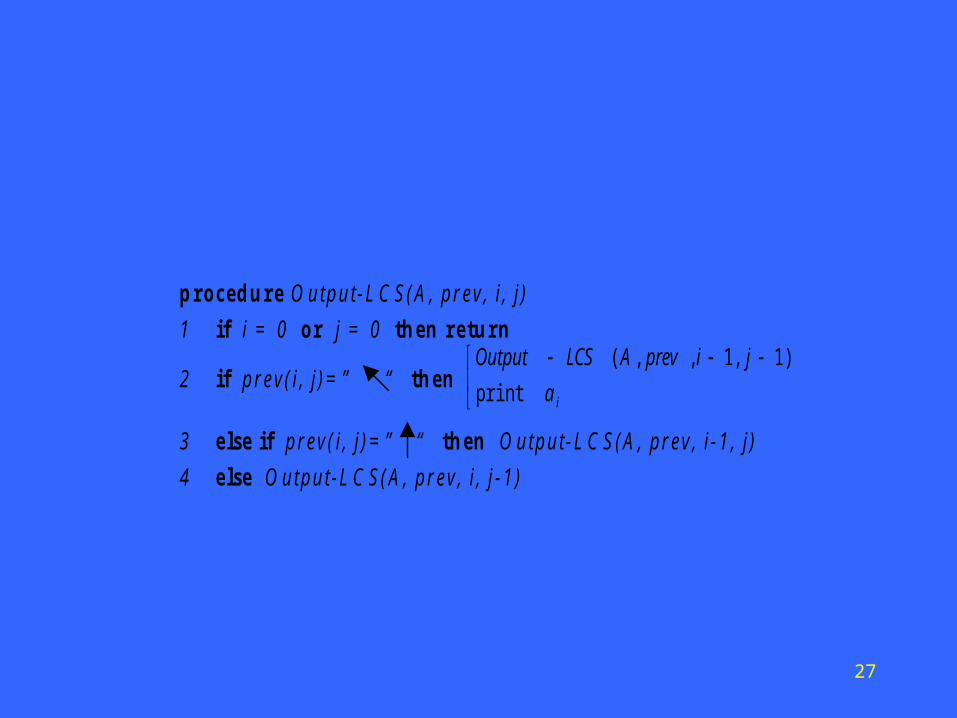
p r o c e d u r e O u tp u t - L C S ( A , p r e v , i , j )
1 i f i = 0 o r j = 0 t h e n r e t u r n
2 i f p r e v ( i , j ) = ” “ t h e n
ia
jiprevALCSOutput
)1,1,,(
3 e l s e i f p r e v ( i , j ) = ” “ t h e n O u tp u t - L C S ( A , p r e v , i - 1 , j )
4 e l s e O u tp u t - L C S ( A , p r e v , i , j - 1 )

28
i j 0 1 p
2 r
3 o
4 v
5 i
6 d
7 e
8 n
9 c
10 e
0 0 0 0 0 0 0 0 0 0 0 0
1 p 2
0 1 1 1 1 1 1 1 1 1 1
2 r 0 1 2 2 2 2 2 2 2 2 2
3 e 0 1 2 2 2 2 2 3 3 3 3
4 s 0 1 2 2 2 2 2 3 3 3 3
5 i 0 1 2 2 2 3 3 3 3 3 3
6 d 0 1 2 2 2 3 4 4 4 4 4
7 e 0 1 2 2 2 3 4 5 5 5 5
8 n 0 1 2 2 2 3 4 5 6 6 6
9 t 0 1 2 2 2 3 4 5 6 6 6
Output: priden

29
Dot MatrixSequence A: CTTAACT
Sequence B: CGGATCATC G G A T C A T
C
T
T
A
A
C
T

30
C---TTAACTCGGATCA--T
Pairwise AlignmentSequence A: CTTAACTSequence B: CGGATCAT
An alignment of A and B:
Sequence A
Sequence B

31
C---TTAACTCGGATCA--T
Pairwise AlignmentSequence A: CTTAACTSequence B: CGGATCAT
An alignment of A and B:
Insertion gap
Match Mismatch
Deletion gap

32
Alignment GraphSequence A: CTTAACT
Sequence B: CGGATCATC G G A T C A T
C
T
T
A
A
C
T
C---TTAACTCGGATCA--T

33
A simple scoring scheme
• Match: +8 (w(x, y) = 8, if x = y)
• Mismatch: -5 (w(x, y) = -5, if x ≠ y)
• Each gap symbol: -3 (w(-,x)=w(x,-)=-3)
C - - - T T A A C TC G G A T C A - - T
+8 -3 -3 -3 +8 -5 +8 -3 -3 +8 = +12
Alignment score

34
An optimal alignment-- the alignment of maximum score
• Let A=a1a2…am and B=b1b2…bn .
• Si,j: the score of an optimal alignment between a1a2…ai and b1b2…bj
• With proper initializations, Si,j can be computedas follows.
),(
),(
),(
max
1,1
1,
,1
,
jiji
jji
iji
ji
baws
bws
aws
s

35
Computing Si,j
i
j
w(ai,-)
w(-,bj)
w(ai,b
j)
Sm,n

36
Initializations
0 -3 -6 -9 -12 -15 -18 -21 -24
-3
-6
-9
-12
-15
-18
-21
C G G A T C A T
C
T
T
A
A
C
T
37
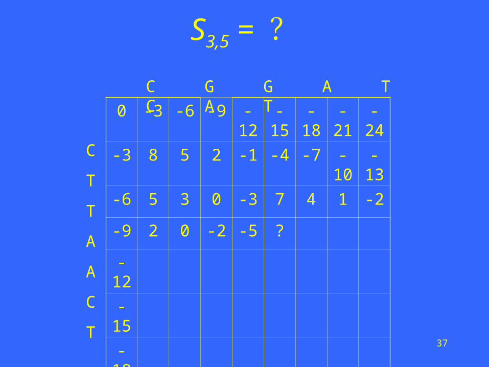
S3,5 = ?
0 -3 -6 -9 -12 -15 -18 -21 -24
-3 8 5 2 -1 -4 -7 -10 -13
-6 5 3 0 -3 7 4 1 -2
-9 2 0 -2 -5 ?
-12
-15
-18
-21
C G G A T C A T
C
T
T
A
A
C
T

38
S3,5 = ?
0 -3 -6 -9 -12 -15 -18 -21 -24
-3 8 5 2 -1 -4 -7 -10 -13
-6 5 3 0 -3 7 4 1 -2
-9 2 0 -2 -5 5 -1 -4 9
-12 -1 -3 -5 6 3 0 7 6
-15 -4 -6 -8 3 1 -2 8 5
-18 -7 -9 -11 0 -2 9 6 3
-21 -10 -12 -14 -3 8 6 4 14
C G G A T C A T
C
T
T
A
A
C
T
optimal score

39
C T T A A C – TC G G A T C A T
0 -3 -6 -9 -12 -15 -18 -21 -24
-3 8 5 2 -1 -4 -7 -10 -13
-6 5 3 0 -3 7 4 1 -2
-9 2 0 -2 -5 5 -1 -4 9
-12 -1 -3 -5 6 3 0 7 6
-15 -4 -6 -8 3 1 -2 8 5
-18 -7 -9 -11 0 -2 9 6 3
-21 -10 -12 -14 -3 8 6 4 14
C G G A T C A T
C
T
T
A
A
C
T
8 – 5 –5 +8 -5 +8 -3 +8 = 14
40
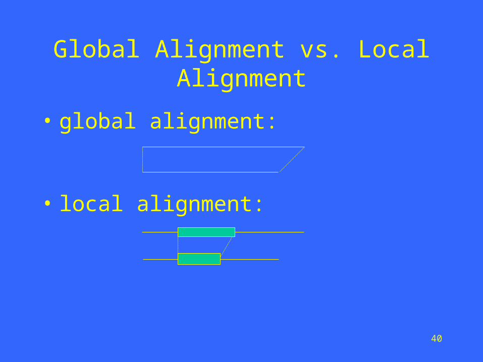
Global Alignment vs. Local Alignment
• global alignment:
• local alignment:
41
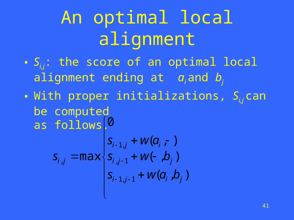
An optimal local alignment
• Si,j: the score of an optimal local alignment ending at ai and bj
• With proper initializations, Si,j can be computedas follows.
),(
),(),(
0
max
1,1
1,
,1
,
jiji
jji
iji
ji
baws
bwsaws
s

42
local alignment
0 0 0 0 0 0 0 0 0
0 8 5 2 0 0 8 5 2
0 5 3 0 0 8 5 3 13
0 2 0 0 0 8 5 2 11
0 0 0 0 8 5 3 ?
0
0
0
C G G A T C A T
C
T
T
A
A
C
T
Match: 8
Mismatch: -5
Gap symbol: -3

43
local alignment
0 0 0 0 0 0 0 0 0
0 8 5 2 0 0 8 5 2
0 5 3 0 0 8 5 3 13
0 2 0 0 0 8 5 2 11
0 0 0 0 8 5 3 13 10
0 0 0 0 8 5 2 11 8
0 8 5 2 5 3 13 10 7
0 5 3 0 2 13 10 8 18
C G G A T C A T
C
T
T
A
A
C
T
Match: 8
Mismatch: -5
Gap symbol: -3
The best
score

44
0 0 0 0 0 0 0 0 0
0 8 5 2 0 0 8 5 2
0 5 3 0 0 8 5 3 13
0 2 0 0 0 8 5 2 11
0 0 0 0 8 5 3 13 10
0 0 0 0 8 5 2 11 8
0 8 5 2 5 3 13 10 7
0 5 3 0 2 13 10 8 18
C G G A T C A T
C
T
T
A
A
C
T
The best
score
A – C - TA T C A T8-3+8-3+8 = 18

45
Affine gap penalties• Match: +8 (w(x, y) = 8, if x = y)
• Mismatch: -5 (w(x, y) = -5, if x ≠ y)
• Each gap symbol: -3 (w(-,x)=w(x,-)=-3)
• Each gap is charged an extra gap-open penalty: -4.
C - - - T T A A C TC G G A T C A - - T
+8 -3 -3 -3 +8 -5 +8 -3 -3 +8 = +12
-4 -4
Alignment score: 12 – 4 – 4 = 4

46
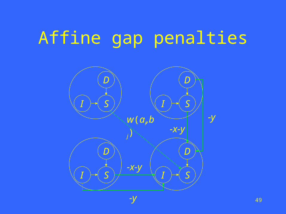
Affine gap penalties
• A gap of length k is penalized x + k·y.
gap-open penalty
gap-symbol penaltyThree cases for alignment endings:
1. ...x...x
2. ...x...-
3. ...-...x
an aligned pair
a deletion
an insertion

47
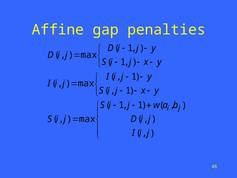
Affine gap penalties
• Let D(i, j) denote the maximum score of any alignment between a1a2…ai and b1b2…bj ending with a deletion.
• Let I(i, j) denote the maximum score of any alignment between a1a2…ai and b1b2…bj ending with an insertion.
• Let S(i, j) denote the maximum score of any alignment between a1a2…ai and b1b2…bj.
48
Affine gap penalties
),(
),(
),()1,1(
max),(
)1,(
)1,(max),(
),1(
),1(max),(
jiI
jiD
bawjiS
jiS
yxjiS
yjiIjiI
yxjiS
yjiDjiD
ji
49
Affine gap penalties
SI
D
SI
D
SI
D
SI
D
-y-x-y
-x-y
-y
w(ai,bj)

50
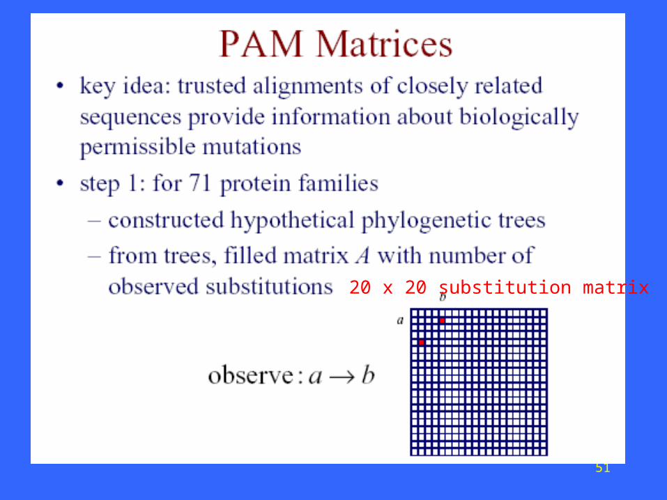
PAM (percent accepted mutation)
• Scoring function is critical element
• above SF is not good enough
• Developing a new scoring function– Based on a set of native protein sequences
51
20 x 20 substitution matrix

52
250
log10 10
k
p
Mscore
b
kab
k
PAM-250

53
PAM –1 The Dayhoff Matrix: Proteins evolve through a succession of independent point mutations, that are accepted in a population and subsequently can be observed in the sequence pool. (Dayhoff, M.O. et al. (1978) Atlas of Protein Sequence and Structure. Vol. 5, Suppl. 3 National Biomedical Research Foundation, Washington D.C. U.S.A).
First step: Pair Exchange Frequencies
A PAM (Percent Accepted Mutation) is one accepted point mutation on the path between two sequences, per 100 residues.

54
PAM –2: Second step: Frequencies of Occurrence of each amino acid
1978 1991L 0.085 0.091A 0.087 0.077G 0.089 0.074S 0.070 0.069V 0.065 0.066E 0.050 0.062T 0.058 0.059K 0.081 0.059I 0.037 0.053D 0.047 0.052R 0.041 0.051P 0.051 0.051N 0.040 0.043Q 0.038 0.041F 0.040 0.040Y 0.030 0.032M 0.015 0.024H 0.034 0.023C 0.033 0.020W 0.010 0.014
aa 20 of one is ,1 apa a
Computing the relative frequency ofoccurrence of a.a. over a large, Sufficiently varied protein sequence seti.e: occurrence in the sample space

55
PAM –3: Third step: Relative Mutabilities
1978 1991A 100 100C 20 44D 106 86E 102 77F 41 51G 49 50H 66 91I 96 103K 56 72L 40 54M 94 93N 134 104P 56 58Q 93 84R 65 83S 120 117T 97 107V 74 98W 18 25Y 41 50
All values are takenrelative to alanine, which is arbitrarily set at 100.
a A.A. theofy probabilit mutation the:
100
mutation ofnumber total:
involveda A.A. theof mutation
ofnumber total:
a
a
aa
a a
a
ab aba
baab
m
fp
fm
f
ff
f
ff
ff

56
PAM –4: Fourth step: Mutation Probability matrix
The probability that an amino acid in row a of the matrix will replace the amino acid in column b : the mutability of amino acid b, multiplied by the pair exchange frequency for aa divided by the sum of all pair exchange frequencies for amino acid a:
aa
ab
ab
mf
f
aaba
baM
changed) Pr()changed |Pr(
)Pr(
Matrix M is a Markov model of evolution

57
PAM –5: Last step: the log-odds matrix
log to base 10: a value of +1 would mean that the corresponding pair has been observed 10 times more frequently than expected by chance. The most commonly used matrix is the matrix from the 1978 edition of the Dayhoff atlas, at PAM 250: this is also frequently referred to as the PAM250 matrix.
bp
baM
p
M
b
ab
b
ab
of occurence random:
tochanged :
b
kab
k p
Mscore 10log10k-PAM defines as

58
250
log10 10
k
p
Mscore
b
kab
k
PAM-250

59
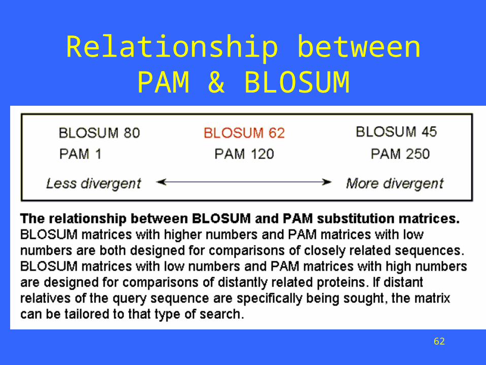
BLOSUM Matrices– BLOSUM matrices are based on local alignments.
– BLOSUM 62 is a matrix calculated from comparisons of sequences with no less than 62% divergence.
– All BLOSUM matrices are based on observed alignments; they are not extrapolated from comparisons of closely related proteins.
– BLOSUM 62 is the default matrix in BLAST 2.0. Though it is tailored for comparisons of moderately distant proteins, it performs well in detecting closer relationships. A search for distant relatives may be more sensitive with a different matrix.

60
BLOSUM62 is the BLAST default

61
A Ala 4
R Arg -1 5
N Asn -2 0 6
D Asp -2 -2 1 6
C Cys 0 -3 -3 -3 9
Q Gln -1 1 0 0 -3 5
E Glu -1 0 0 2 -4 2 5
G Gly 0 -2 0 -1 -3 -2 -2 6
H His -2 0 1 -1 -3 0 0 -2 8
I Ile -1 -3 -3 -3 -1 -3 -3 -4 -3 4
L Leu -1 -2 -3 -4 -1 -2 -3 -4 -3 2 4
K Lys -1 2 0 -1 -3 1 1 -2 -1 -3 -2 5
M Met -1 -1 -2 -3 -1 0 -2 -3 -2 1 2 -1 5
F Phe -2 -3 -3 -3 -2 -3 -3 -3 -1 0 0 -3 0 6
P Pro -1 -2 -2 -1 -3 -1 -1 -2 -2 -3 -3 -1 -2 -4 7
S Ser 1 -1 1 0 -1 0 0 0 -1 -2 -2 0 -1 -2 -1 4
T Thr 0 -1 0 -1 -1 -1 -1 -2 -2 -1 -1 -1 -1 -2 -1 1 5
W Trp -3 -3 -4 -4 -2 -2 -3 -2 -2 -3 -2 -3 -1 1 -4 -3 -2 11
Y Tyr -2 -2 -2 -3 -2 -1 -2 -3 2 -1 -1 -2 -1 3 -3 -2 -2 2 7
V Val 0 -3 -3 -3 -1 -2 -2 -3 -3 3 1 -2 1 -1 -2 -2 0 -3 -1 4
Ala Arg Asn Asp Cys Gln Glu Gly His Ile Leu Lys Met Phe Pro Ser Thr Trp Tyr Val
A R N D C Q E G H I L K M F P S T W Y V
BLOSUM 62
62
Relationship between PAM & BLOSUM

63
Gap Penalty
Query Length Substitution Matrix Gap Costs<35 PAM-30 (9,1)35-50 PAM-70 (10,1)50-85 BLOSUM-80 (10,1)>85 BLOSUM-62 (10,1)

64
k best local alignments
• Smith-Waterman(Smith and Waterman, 1981; Waterman and Eggert, 1987)– linear-space version: sim (Huang and Miller, 1991)
– linear-space variants: sim2 (Chao et al., 1995); sim3 (Chao et al., 1997)
• FASTA(Wilbur and Lipman, 1983; Lipman and Pearson, 1985)– linear-space band alignment (Chao et al., 1992)
• BLAST(Altschul et al., 1990; Altschul et al., 1997)– restricted affine gap penalties (Chao, 1999)

65
FASTA
1) Find runs of identities, and identify regions with the highest density of identities.
2) Re-score using PAM matrix, and keep top scoring segments.
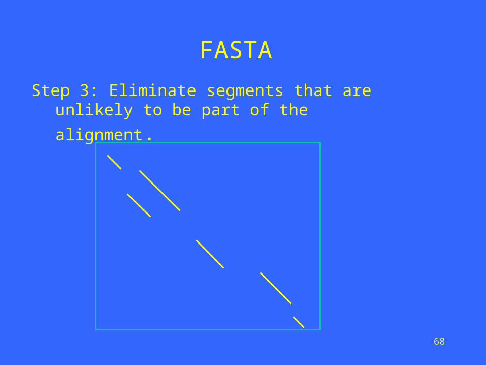
3) Eliminate segments that are unlikely to be part of the alignment.
4) Optimize the alignment in a band.

66
FASTA
Step 1: Find runes of identities, and identify regions with the highest density of identities.

67
FASTA
Step 2: Re-score using PAM matrix, andkeep top scoring segments.
68
FASTA
Step 3: Eliminate segments that are unlikely to be part
of the alignment.

69
FASTA
Step 4: Optimize the alignment in a band.

70
BLAST
1) Build the hash table for Sequence A.
2) Scan Sequence B for hits.
3) Extend hits.

71
BLASTStep 1: Build the hash table for Sequence A. (3-tuple example)
For DNA sequences:
Seq. A = AGATCGAT 12345678AAAAAC..AGA 1..ATC 3..CGA 5..GAT 2 6..TCG 4..
TTT
For protein sequences:
Seq. A = ELVIS
Add xyz to the hash table if Score(xyz, ELV) T;≧Add xyz to the hash table if Score(xyz, LVI) T;≧Add xyz to the hash table if Score(xyz, VIS) T;≧

72
BLASTStep2: Scan sequence B for hits.

73
BLASTStep2: Scan sequence B for hits.
Step 3: Extend hits.
hit
Terminate if the score of the sxtension fades away.
BLAST 2.0 saves the time spent in extension, and
considers gapped alignments.

74
Remarks
• Filtering is based on the observation that a good alignment usually includes short identical or very similar fragments.
• The idea of filtration was used in both FASTA and BLAST.

75
Linear-space ideasHirschberg, 1975; Myers and Miller, 1988
m/2

76
Two subproblems½ original problem size
m/2
m/4
3m/4

77
Four subproblems¼ original problem size
m/2
m/4
3m/4
78
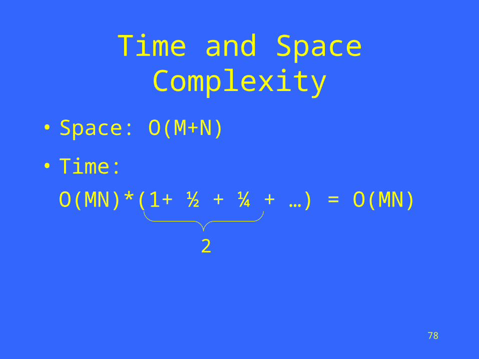
Time and Space Complexity
• Space: O(M+N)
• Time:
O(MN)*(1+ ½ + ¼ + …) = O(MN)
2

79
Band Alignment
Sequence B
Sequence A

80
Band Alignment in Linear Space
The remaining subproblems are no longer only half of the original problem. In worst case, this could cause an additional log n factor in time.

81
Band Alignment in Linear Space

82
Multiple sequence alignment (MSA)
• The multiple sequence alignment problem is to simultaneously align more than two sequences.
Seq1: GCTC
Seq2: AC
Seq3: GATC
GC-TC
A---C
G-ATC
83
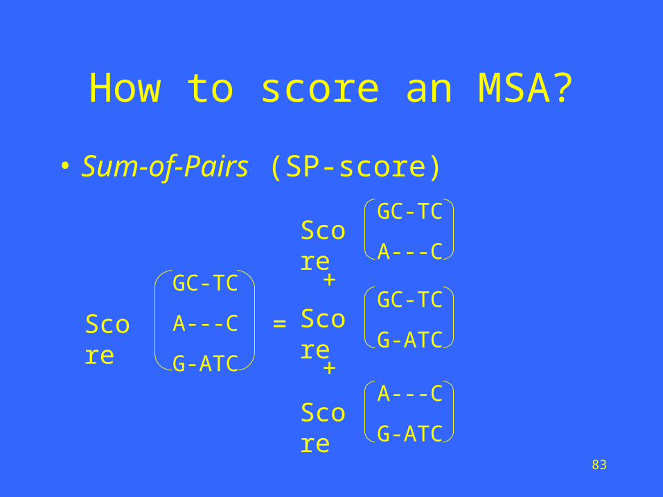
How to score an MSA?
• Sum-of-Pairs (SP-score)
GC-TC
A---C
G-ATC
GC-TC
A---C
GC-TC
G-ATC
A---C
G-ATC
Score =
Score
Score
Score
+
+

84
Defining scores for alignment columns
• infocon [Stojanovic et al., 1999]– Each column is assigned a score that measures its infor
mation content, based on the frequencies of the letters both within the column and within the alignment.
CGGATCAT—GGACTTAACATTGAAGAGAACATAGTA

85
Defining scores (cont’d)
• phylogen [Stojanovic et al., 1999]– columns are scored based on the evolutionary r
elationships among the sequences implied by a supplied phylogenetic tree.
TTTCC T T T C C
CT
TT
T T T C C
T T
TT
Score = 1 Score = 2
86
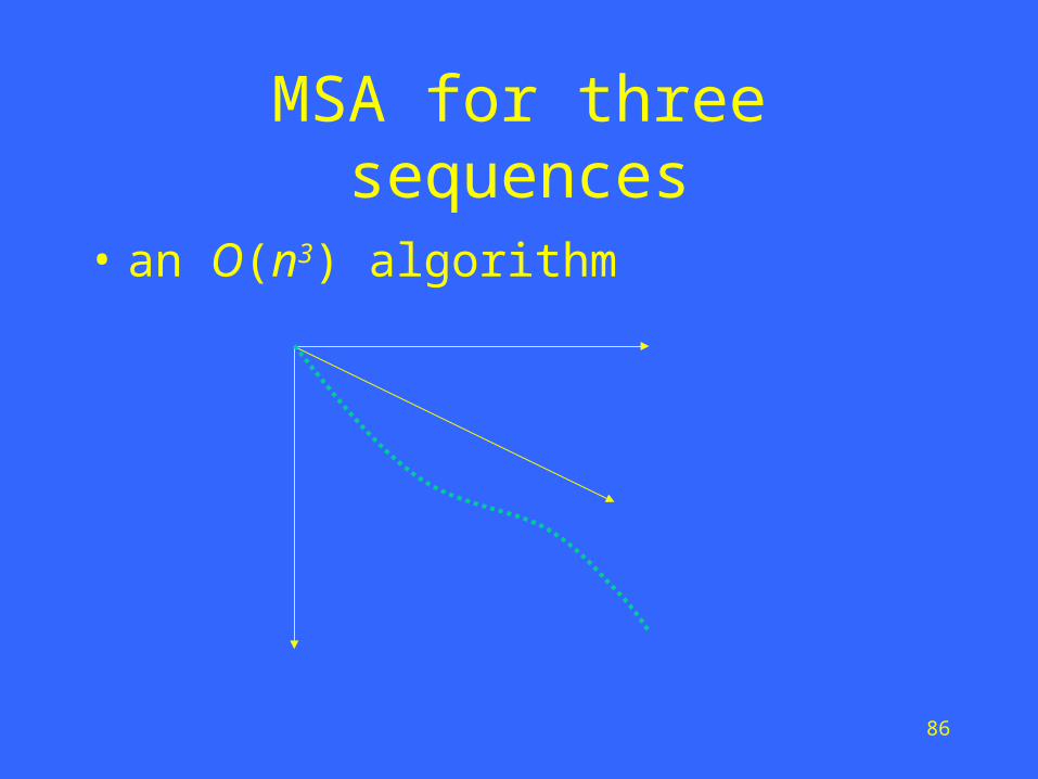
MSA for three sequences
• an O(n3) algorithm

87
General MSA
• For k sequences of length n: O(nk)
• NP-Complete (Wang and Jiang)
• The exact multiple alignment algorithms for many sequences are not feasible.
• Some approximation algorithms are given.(e.g., 2- l/k for any fixed l by Bafna et al.)

88
Progressive alignment
• A heuristic approach proposed by Feng and Doolittle.• It iteratively merges the most similar pairs.• “Once a gap, always a gap”
A B C D E
The time for progressive alignment in most cases is roughly the order of the time for computing all pairwise alignme
nt, i.e., O(k2n2) .

89
Concluding remarks
• Three essential components of the dynamic-programming approach:– the recurrence relation– the tabular computation– the traceback
• The dynamic-programming approach has been used in a vast number of computational problems in bioinformatics.


![New frontiers in atomic force microscopy: analyzing interactions from single … · 2014. 8. 19. · measuring biomolecular forces, including the osmotic stress method [1], the surface](https://img.pdfslide.net/doc/110x75/61254f8da8a80b45b314aacb/new-frontiers-in-atomic-force-microscopy-analyzing-interactions-from-single-2014.jpg)