Dynamic Programming Strategies on the Decision Tree … · a clear tool for their study and classiﬁcation which can help in the comprehension of the essence of this programming

Informatics in Education, 2007, Vol. 6, No. 1, 115–138 115© 2007 Institute of Mathematics and Informatics, Vilnius

Dynamic Programming Strategies on the DecisionTree Hidden behind the Optimizing Problems

Zoltan KATAIMathematics and Informatics Department, Sapientia Hungarian University of TransylvaniaBd. 1848, 58/30, 540398, Targu Mures, Romaniae-mail: [email protected]

Received: April 2006

Abstract. The aim of the paper is to present the characteristics of certain dynamic programmingstrategies on the decision tree hidden behind the optimizing problems and thus to offer such a cleartool for their study and classification which can help in the comprehension of the essence of thisprogramming technique.

Key words: dynamic programming, programming techniques, decision trees.

Introduction

Several books treat the problem of dynamic programming by presenting the principlesstanding at the basis of the technique and then giving a few examples of solved prob-lems. For instance the book called Algorithms by Cormen, Leiserson and Rivest (1990),mentions the optimal substructures and the overlapped subproblems as elements of thedynamic programming. Razvan Andone and Ilie Garbacea (1995) are talking about thethree basic principles of the dynamic programming in their book Basic Algorithms:

1) avoid the repeated solving of identical subproblems by saving the optimal subsolu-tions;

2) we solve the subproblems advancing from the simple toward the complex;3) the principle of optimality.

The book Programming Techniques by Tudor Sorin (1997) gives a certain classifica-tion of the dynamic programming strategies: forwards method, backwards method andmixed method.

In this paper we would like to go further in the study and classification of the dynamicprogramming strategies. By presenting the characteristics of certain dynamic program-ming strategies on the decision tree hidden behind the optimizing problems we offer sucha clear tool for their study and classification which can help in the comprehension of theessence of this programming technique.

116 Z. Katai

The Decision Tree

Dynamic programming is often used to solve optimizing problems. Usually the problemconsists on a target function which has to be optimized through a sequence of (optimal)decisions. For each optimizing problem a rooted tree (tree structure) can be ordered,which will be called decision tree. The root represents the starting state of the problem,the first level nodes represent the states the problem can reach after the first decision, thesecond level nodes those reached after the second decision etc. A node will have as manysons as the number of possible choices for the respective decision.

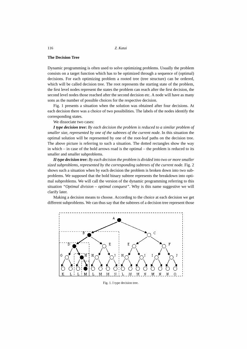
Fig. 1 presents a situation when the solution was obtained after four decisions. Ateach decision there was a choice of two possibilities. The labels of the nodes identify thecorresponding states.

We dissociate two cases:I type decision tree: By each decision the problem is reduced to a similar problem of

smaller size, represented by one of the subtrees of the current node. In this situation theoptimal solution will be represented by one of the root-leaf paths on the decision tree.The above picture is referring to such a situation. The dotted rectangles show the wayin which – in case of the bold arrows road is the optimal – the problem is reduced to itssmaller and smaller subproblems.

II type decision tree: By each decision the problem is divided into two or more smallersized subproblems, represented by the corresponding subtrees of the current node. Fig. 2shows such a situation when by each decision the problem is broken down into two sub-problems. We supposed that the bold binary subtree represents the breakdown into opti-mal subproblems. We will call the version of the dynamic programming referring to thissituation “Optimal division – optimal conquest”. Why is this name suggestive we willclarify later.

Making a decision means to choose. According to the choice at each decision we getdifferent subproblems. We can thus say that the subtrees of a decision tree represent those

Fig. 1. I type decision tree.

Dynamic Programming Strategies on the Decision Tree 117

Fig. 2. II type decision tree.

subproblems the problem can be reduced to (case 1), respectively broken down (case 2)through certain sequences of decisions.

Considering the fact that the subproblems are similar, we can speak about their generalform. By general form we always mean a form with parameters. To comprehend thestructure of a problem means, amongst others, to clarify the followings:

• what is the general form of the subproblems,• which parameters describe this,• which are the parameter values for which we get the original problem, respectively

the trivial subproblems as marginal cases of the general problem.

The Contracted Decision Tree

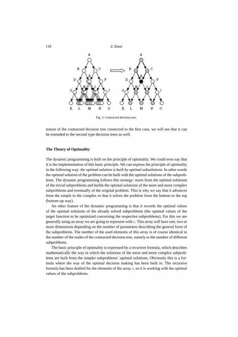
Although the number of the decision tree’s nodes depends exponentially on the numberof the decisions of the optimal sequence of decisions, it often happens that it containsseveral identical nodes, which obviously represent identical states and which are of coursecharacterized by the same parameter values. (As we will later see, the bigger the numberof identical nodes, the more can the dynamic programming make use of its strengths.) Incase of the first type decision trees this situation occurs when the problem is reduced tothe same subproblem by means of different subsequences of decisions. Such a situationis represented by the decision tree shown in Fig. 1. We overlap the nodes representing theidentical states of the tree (see Fig. 3). We called the obtained data structure contracteddecision tree.

As we can see, the contracted decision tree is not a tree structure any more, but adigraph. The contracted tree will have exactly as many nodes as the number of differentstates the problem can get (this number is usually only a polynomial function of thenumber of decisions leading to the optimal solution.). Although we have presented the

118 Z. Katai

Fig. 3. Contracted decision tree.

notion of the contracted decision tree connected to the first case, we will see that it canbe extended to the second type decision trees as well.

The Theory of Optimality

The dynamic programming is built on the principle of optimality. We could even say thatit is the implementation of this basic principle. We can express the principle of optimalityin the following way: the optimal solution is built by optimal subsolutions. In other wordsthe optimal solution of the problem can be built with the optimal solutions of the subprob-lems. The dynamic programming follows this strategy: starts from the optimal solutionsof the trivial subproblems and builds the optimal solutions of the more and more complexsubproblems and eventually of the original problem. This is why we say that it advancesfrom the simple to the complex or that it solves the problem from the bottom to the top(bottom-up way).

An other feature of the dynamic programming is that it records the optimal valuesof the optimal solutions of the already solved subproblems (the optimal values of thetarget function to be optimized concerning the respective subproblems). For this we aregenerally using an array we are going to represent with c. This array will have one, two ormore dimensions depending on the number of parameters describing the general form ofthe subproblems. The number of the used elements of this array is of course identical tothe number of the nodes of the contracted decision tree, namely to the number of differentsubproblems.

The basic principle of optimality is expressed by a recursive formula, which describesmathematically the way in which the solutions of the more and more complex subprob-lems are built from the simpler subproblems’ optimal solutions. Obviously this is a for-mula where the way of the optimal decision making has been built in. The recursiveformula has been drafted for the elements of the array c, so it is working with the optimalvalues of the subproblems.


How is the implementation of the basic principle of optimality reflected on the decisiontree, on the contracted decision tree, respectively on the array storing the optimal valuesof the subproblems?

1. If nodes representing identical states appear on the crown of the growing decisiontree, it will grow only in the direction of the branch representing the optimal solu-tion of the respective subproblem.

2. We prune the nodes of the contracted decision tree, in the order dictated by therecursive formula, in such a manner that there should be only one path to each ofthem, namely the one representing the optimal solution.

3. The core of the algorithm is represented by the filling of the corresponding el-ements of the c array according to the strategy given by the recursive formula.Although the c array stores one to one only the optimal values of the subproblems,still it contains enough information to reconstruct the sequence of the optimal de-cisions. It is often suitable to somehow store the optimal choices themselves whenfilling the array c. This could facilitate or even make faster the reconstruction ofthe optimal decision-sequence.

When the principle of optimality is valid for a problem, this could considerably re-duce the time necessary to build the optimal solution, because in building it we can relyexclusively on the optimal solutions of the subproblems.

Dynamic Programming on the I Type Decision Tree

Let’s picture to ourselves again the first type decision tree. The root represents the start-ing state, when the whole problem needs to be solved. The solution-leaves of the treerepresent the solved states of the problem and the root-solutionleaf paths represent thepotential solutions (the wanted optimal solution is to be found among them). In the inter-mediate states represented by the nodes of the tree the problem contains a part which hasalready been solved and one which needs to be solved. We call these the prefix and suffixsubproblems of the respective state.

The path leading to a given node represents the sequence of decisions leading to thecorresponding state. This sequence of decisions can be considered as one solution of theprefix subproblem of the respective state. The different sequences of decisions leadingto the identical nodes overlapped in the contracted decision tree can be considered asdifferent solutions of the corresponding prefix subproblem.

The suffix subproblem of a state (this is nothing else but the subproblem the problemin the respective state has been reduced to) – as we have already referred to it – is repre-sented in the decision tree by the subtree of the corresponding node (that one whose rootis the node). The solutions of the suffix type subproblems are obviously represented bythe root-leaf paths of the corresponding subtree. On picture number 3 the solutions of theprefix problem of state are bold, the edges of the subtree representing the correspondingsuffix problem are dotted.

120 Z. Katai

The optimal solutions of the prefix respectively suffix problems belonging to the samestate in the contracted tree will be represented by the optimal root-node path connectedto the respective node, respectively the optimal node-leaf path.

We can distinguish two subcases, should the contracted decision tree, as a directedgraph, contents or not cycles.

If the Contracted Decision Tree is Cycle Free

What does it mean to advance from simple towards the complex (from bottom to top)?From the point of view of the prefix subproblems, from bottom to top means the root-leaves direction. Considering the suffix problems, they are growing in the opposite di-rection, from the leaves towards the root. This duality leads to the two versions of thedynamic programming:

1. Root-leaves directed dynamic programming (Method Forwards).2. Leaves-root directed dynamic programming (Method Backwards).

Should D1, D2, . . . , Di−1, Di, Di+1, . . . , Dn be the optimal sequence of decisions(in the decision tree this is leading along the root-leaf path representing the optimal so-lution). Let us suppose that this sequence of decisions, starting from the original stateS0 (represented by the root of the tree), “goes through” the states S1, S2, . . . , Si, . . . , Sn

(state Sn is represented by the tree’s “optimal leaf”). The above mentioned two versionsof the dynamic programming uses the basic principle of the optimality in the followingforms:

Assuming that D1, D2, . . . , Dn is the optimal sequence of decisions meaning the so-lution of the problem, then

1) subsequences of decisions bearing the form D1, D2, . . . , Di (i = 1, n−1) are alsooptimal,

2) subsequences of decisions bearing the form Di, Di+1, . . . , Dn (i = 2, n) are alsooptimal.

In order to have a better view of these strategies, we apply them for the followingproblem.

Triangle: On the main diagonal and in the triangle under the main diagonal of asquare matrix with n rows there are natural numbers. We assume that the matrix is storedin a bidimensional array a. Determine the “the longest” path from peak (element a[1][1])to the base (n-th row), considering the following:

• on a certain path element a[i][j] can be followed either by element a[i + 1][j](down), or by element a[i + 1][j + 1] (diagonally to the right), where 1 � i < n

and 1 � j < n;• by the “length” of a path we mean the sum of the elements to be found along the

path.

For example, should for n = 5 the matrix be the following (see Fig. 4), then the“longest” path from the peak to the base is the shaded one, its length is 37.

The following decision tree can be associated to the problem (see Fig. 5).


Fig. 4. Array a associated to the triangle problem.

Fig. 5. The decision tree associated to the triangle problem.

The general prefix problem:Determine the optimal path from the peak to position (i, j).

The general suffix problem:Determine the optimal path from position (i, j) to the base.

So the parameters of the problem are i and j. We can see that the decision tree hasnodes with the same corresponding parameter values. Obviously these nodes representidentical states, with the same associated prefix respectively suffix problem. We overlapthe nodes representing identical states. We get the attached contracted decision tree. Wesee it also built into the array (see Figs. 6 and 7).

As the subproblems are determined by two independent parameters, we use a bidi-mensional array (more exactly, the elements of the array situated on the main diagonaland under it) to store the optimal values belonging to their optimal solutions. It can benoticed that the number of the nodes of the contracted decision tree is the same as thenumber of the used elements of the array chosen for the storage.

122 Z. Katai

Fig. 6. The contracted decision tree attached to the triangle problem.

Fig. 7. The contracted decision tree built into the array.

In the root-leaves oriented version the element c[i][j] of the array stores the optimalvalue of the prefix problem associated to state (i, j), namely the length of the optimalpath leading from the peak to the element with position (i, j). Opposed to that, in theleaves-root oriented version the length of the best path leading from position (i, j) to thebase gets into the element c[i][j] of the array, which represents the optimal value of thesuffix problem.


Root-leaves Oriented Dynamic Programming

We prune every node advancing from the root towards the leaves, leaving only “the best”father-branch, the one traversed by the optimal solution of the prefix problem of the re-spective node. What has been marked on the Fig. 8 is only one of the possible orders ofpruning. The basic requirement is that when a node is the next one in order, its father-nodes should have already been pruned before. We could say that we tackle the nodesin a topological order. Since the contracted decision tree, as a digraph, is cycle free, thisorder exists.

The implementation of the above presented algorithm means to fill up the elements ofarray c – in topological order, according to the following recursive formula (see Figs. 9and 10):

c[1][1] = a[1][1],

c[i][1] = a[i][1] + c[i − 1][1], 2 � i � n,

c[i][j] = a[i][j] + max(c[i − 1][j], c[i − 1][j − 1]), 2 � i � n, 2 � j � i.

The elements of row n of array c store the length of the best paths from the peak tothe respective positions. Obviously the biggest one represents the length of the best pathfrom the peak to the base. If we would like to get the optimal path itself, array c contains

Fig. 8. A possible prune order of the contracted decision tree in case of the root-leaves oriented dynamicprogramming.

124 Z. Katai

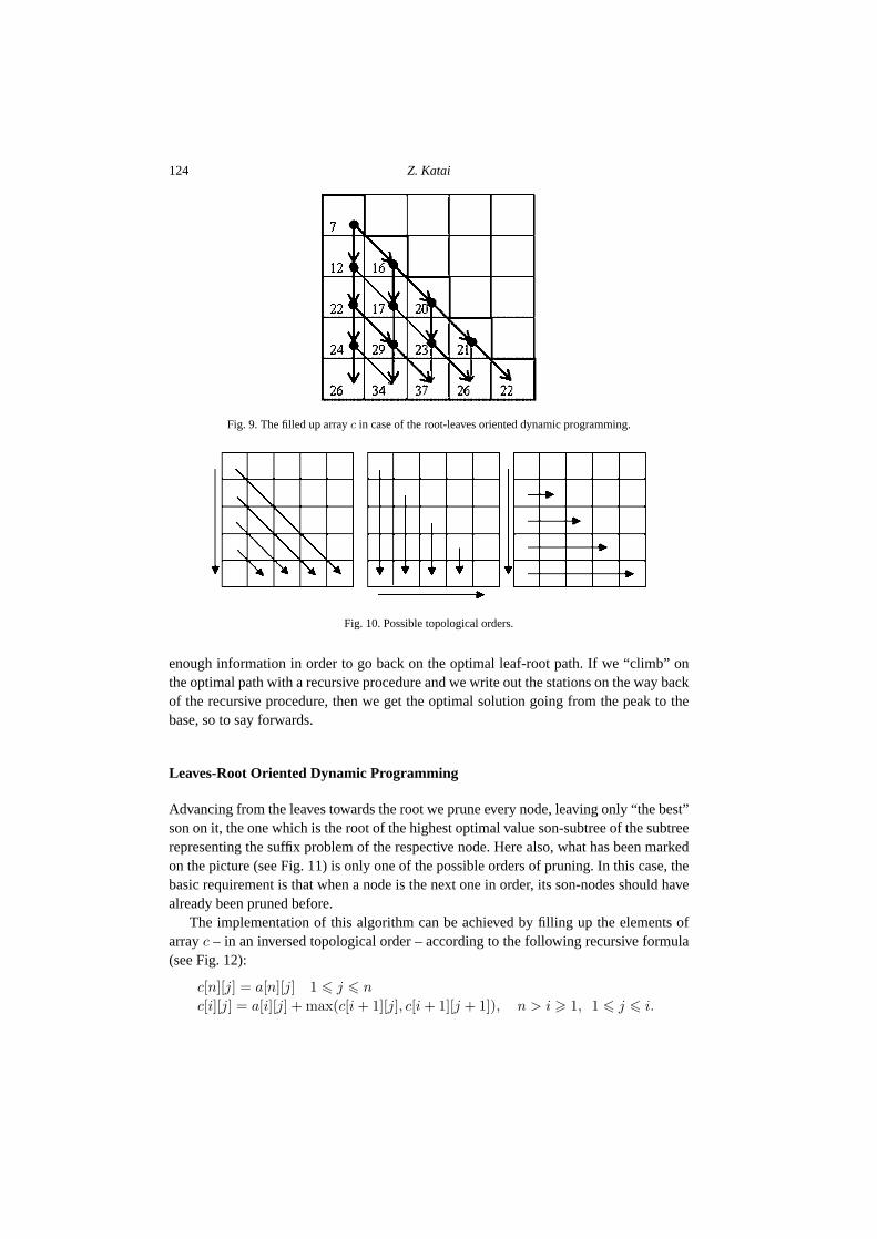
Fig. 9. The filled up array c in case of the root-leaves oriented dynamic programming.

Fig. 10. Possible topological orders.

enough information in order to go back on the optimal leaf-root path. If we “climb” onthe optimal path with a recursive procedure and we write out the stations on the way backof the recursive procedure, then we get the optimal solution going from the peak to thebase, so to say forwards.

Leaves-Root Oriented Dynamic Programming

Advancing from the leaves towards the root we prune every node, leaving only “the best”son on it, the one which is the root of the highest optimal value son-subtree of the subtreerepresenting the suffix problem of the respective node. Here also, what has been markedon the picture (see Fig. 11) is only one of the possible orders of pruning. In this case, thebasic requirement is that when a node is the next one in order, its son-nodes should havealready been pruned before.

The implementation of this algorithm can be achieved by filling up the elements ofarray c – in an inversed topological order – according to the following recursive formula(see Fig. 12):

c[n][j] = a[n][j] 1 � j � n

c[i][j] = a[i][j] + max(c[i + 1][j], c[i + 1][j + 1]), n > i � 1, 1 � j � i.


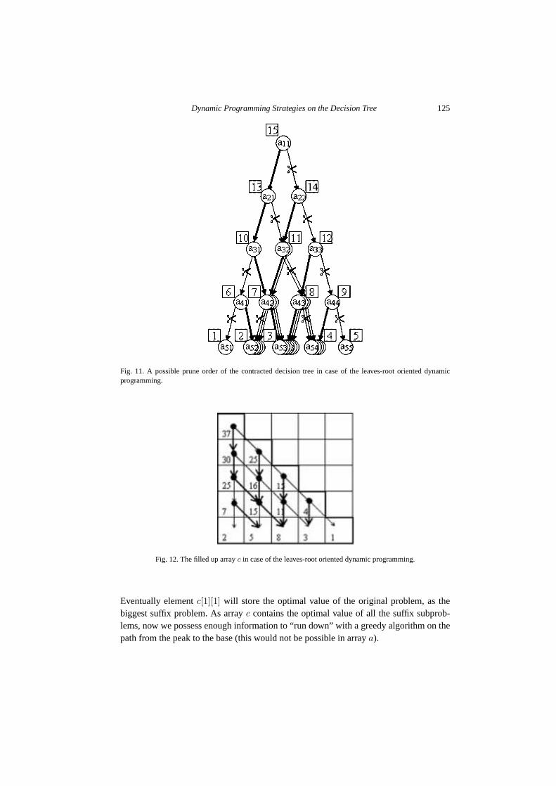
Fig. 11. A possible prune order of the contracted decision tree in case of the leaves-root oriented dynamicprogramming.

Fig. 12. The filled up array c in case of the leaves-root oriented dynamic programming.

Eventually element c[1][1] will store the optimal value of the original problem, as thebiggest suffix problem. As array c contains the optimal value of all the suffix subprob-lems, now we possess enough information to “run down” with a greedy algorithm on thepath from the peak to the base (this would not be possible in array a).

126 Z. Katai

When the Contracted Decision Tree Contents Cycles

Let’s see now a situation when the contracted tree, as a digraph, contents cycles. For thiswe have the following problem:

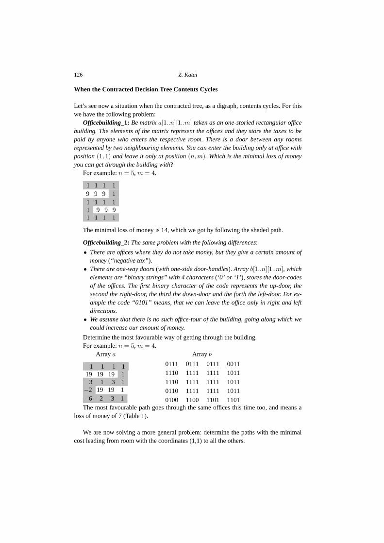
Officebuilding_1: Be matrix a[1..n][1..m] taken as an one-storied rectangular officebuilding. The elements of the matrix represent the offices and they store the taxes to bepaid by anyone who enters the respective room. There is a door between any roomsrepresented by two neighbouring elements. You can enter the building only at office withposition (1, 1) and leave it only at position (n, m). Which is the minimal loss of moneyyou can get through the building with?

For example: n = 5, m = 4.

1 1 1 19 9 9 11 1 1 11 9 9 91 1 1 1

The minimal loss of money is 14, which we got by following the shaded path.

Officebuilding_2: The same problem with the following differences:

• There are offices where they do not take money, but they give a certain amount ofmoney (“negative tax”).

• There are one-way doors (with one-side door-handles). Array b[1..n][1..m], whichelements are “binary strings” with 4 characters (‘0’ or ‘1’), stores the door-codesof the offices. The first binary character of the code represents the up-door, thesecond the right-door, the third the down-door and the forth the left-door. For ex-ample the code “0101” means, that we can leave the office only in right and leftdirections.

• We assume that there is no such office-tour of the building, going along which wecould increase our amount of money.

Determine the most favourable way of getting through the building.For example: n = 5, m = 4.

Array a Array b

1 1 1 119 19 19 1

3 1 3 1−2 19 19 1−6 −2 3 1

0111 0111 0111 0011

1110 1111 1111 1011

1110 1111 1111 1011

0110 1111 1111 1011

0100 1100 1101 1101The most favourable path goes through the same offices this time too, and means a

loss of money of 7 (Table 1).

We are now solving a more general problem: determine the paths with the minimalcost leading from room with the coordinates (1,1) to all the others.


Table 1

Officebuilding_2 with doors and tax values

0 0 0 0... 1 1 1 1 1 1 1 1 1 1 1 0

1 1 1 1

1 1 1 1

0 19 1 1 19 1 1 19 1 1 1 0

1 1 1 1

1 1 1 1

0 3 1 1 1 1 1 3 1 1 1 0

1 1 1 1

0 1 1 1

0 – 2 1 1 19 1 1 19 1 1 1 0

1 1 1 1

0 1 1 1...0 – 6 1 1 – 2 1 1 3 1 1 1 1

0 0 0 0

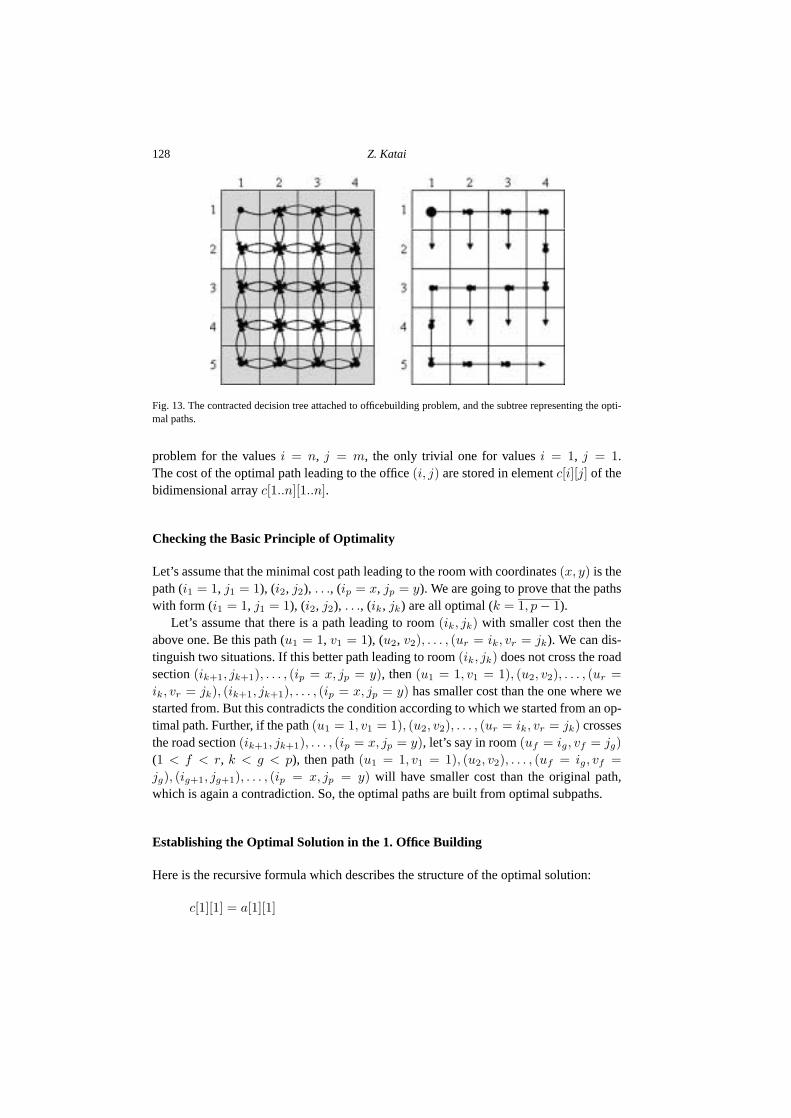
As we are looking for the path with the minimal cost we can state that it must have noloops. The root of the tree structure (decision tree) which can be associated to the prob-lem obviously represents the office with position (1,1). Certain nodes will have as manysons, as the number of directions that can be taken from the respective office withoutmaking any loops. The leaves represent the end of the deadlocks. The optimal solution isrepresented by the path with minimal cost out of the paths leading from the root to thenodes representing the office with position (n,m). Although we cannot draw the abovedescribed decision tree due to lack of space, it is not difficult to notice that it has severalidentical nodes (the nodes are identified by the coordinates of the represented offices).

We overlap the identical nodes. The contracted decision tree thus obtained (see bel-low), as digraph, contents cycle any more. This is due to the fact that the ancestor-offspring relationship between the nodes in the decision tree is not permanent. For ex-ample, the node (1,2) is on certain branches ancestor of the node (2,2) ((1,1), (1,2), (2,2),. . .), on other branches the situation is opposite, node (2,2) is the ancestor of (1,2) ((1,1),(2,1), (2,2), (1,2), . . .). Because of this, there will be a return path in the contracted deci-sion tree between nodes (1,2) and (2,2).

Therefore the problem might be stated in the following way: determine the path withthe minimal cost leading from node (1,1) of the contracted decision tree to node (n,m) (ingeneral to all the other nodes). On the Fig. 13 we have bolded the edges of the optimalpath, respectively we have shaded the corresponding offices. On the picture from theright (see Fig. 13) we have highlighted from the decision tree the subtree representingthe optimal paths from the left upper corner office to all the others, applied to problemofficebuilding_1.

We can consider as a general subproblem the determination of the minimal cost pathleading from the left upper corner to the office with position (i, j). We get the original

128 Z. Katai

Fig. 13. The contracted decision tree attached to officebuilding problem, and the subtree representing the opti-mal paths.

problem for the values i = n, j = m, the only trivial one for values i = 1, j = 1.The cost of the optimal path leading to the office (i, j) are stored in element c[i][j] of thebidimensional array c[1..n][1..n].

Checking the Basic Principle of Optimality

Let’s assume that the minimal cost path leading to the room with coordinates (x, y) is thepath (i1 = 1, j1 = 1), (i2, j2), . . ., (ip = x, jp = y). We are going to prove that the pathswith form (i1 = 1, j1 = 1), (i2, j2), . . ., (ik, jk) are all optimal (k = 1, p − 1).

Let’s assume that there is a path leading to room (ik, jk) with smaller cost then theabove one. Be this path (u1 = 1, v1 = 1), (u2, v2), . . . , (ur = ik, vr = jk). We can dis-tinguish two situations. If this better path leading to room (ik, jk) does not cross the roadsection (ik+1, jk+1), . . . , (ip = x, jp = y), then (u1 = 1, v1 = 1), (u2, v2), . . . , (ur =ik, vr = jk), (ik+1, jk+1), . . . , (ip = x, jp = y) has smaller cost than the one where westarted from. But this contradicts the condition according to which we started from an op-timal path. Further, if the path (u1 = 1, v1 = 1), (u2, v2), . . . , (ur = ik, vr = jk) crossesthe road section (ik+1, jk+1), . . . , (ip = x, jp = y), let’s say in room (uf = ig, vf = jg)(1 < f < r, k < g < p), then path (u1 = 1, v1 = 1), (u2, v2), . . . , (uf = ig, vf =jg), (ig+1, jg+1), . . . , (ip = x, jp = y) will have smaller cost than the original path,which is again a contradiction. So, the optimal paths are built from optimal subpaths.

Establishing the Optimal Solution in the 1. Office Building

Here is the recursive formula which describes the structure of the optimal solution:

c[1][1] = a[1][1]


otherwise

c[i][j] = a[i][j]

+ min(c[i − 1][j], c[i][j + 1], c[i + 1][j], c[i][j − 1])

assuming that the rooms with the respective positions exist

As we can see, we haven’t charged the general formula with conditions refering toparameters i and j. It is well perceptible from the pictures from which directions can weenter into certain rooms.

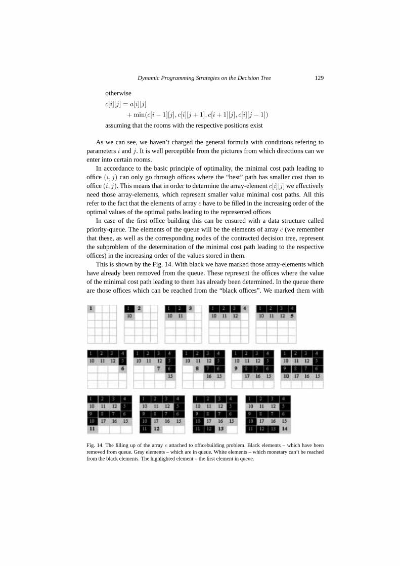
In accordance to the basic principle of optimality, the minimal cost path leading tooffice (i, j) can only go through offices where the “best” path has smaller cost than tooffice (i, j). This means that in order to determine the array-element c[i][j] we effectivelyneed those array-elements, which represent smaller value minimal cost paths. All thisrefer to the fact that the elements of array c have to be filled in the increasing order of theoptimal values of the optimal paths leading to the represented offices

In case of the first office building this can be ensured with a data structure calledpriority-queue. The elements of the queue will be the elements of array c (we rememberthat these, as well as the corresponding nodes of the contracted decision tree, representthe subproblem of the determination of the minimal cost path leading to the respectiveoffices) in the increasing order of the values stored in them.

This is shown by the Fig. 14. With black we have marked those array-elements whichhave already been removed from the queue. These represent the offices where the valueof the minimal cost path leading to them has already been determined. In the queue thereare those offices which can be reached from the “black offices”. We marked them with

Fig. 14. The filling up of the array c attached to officebuilding problem. Black elements – which have beenremoved from queue. Gray elements – which are in queue. White elements – which monetary can’t be reachedfrom the black elements. The highlighted element – the first element in queue.

130 Z. Katai

grey. The elements corresponding to the “grey offices” store the minimal costs we can getto them with, crossing exclusively black rooms. We have highlighted the highest priorityelement of the queue, the “first in the queue”. We have left white those offices whichcannot be reached through the black offices.

At the beginning the queue-structure contains the office with position (1,1). This isreflected in the array by making element c[1][1] grey and it is filled with the value a[1][1](this is the tax claimed in this office). Following this, the algorithm executes at each stepthe following operations on the office which is first in the queue (should its coordinatesbe (i e, j e)):

• It changes the colour of the office which is the first in the queue into black, (thus it iserased from the queue, as one to which the minimal cost path has been found). It isobvious that the value c[i e][j e] represents a minimal cost path from the fact thatall the other offices (the grey ones and the white ones) either cannot be reachedthrough the offices which are already black (the white ones) or they can only bereached on more expensive paths (the other grey ones).

• Should the office which is the first in the queue have such a grey neighbour towhich there is a path through it with a lower cost than the one crossing the officesbeing black until now, then we refresh the corresponding array-element (thus therespective office obviously advances in the priority list). If we mark the position ofthe respective grey neighbour with (i sz, j sz) then the operation is the following:if c[i_e][j_e]+a[i_sz][j_sz]>c[i_sz][j_sz] thenc[i_sz][j_sz]=c[i_e][j_e]+a[i_sz][j_sz]end ifIn the case of this problem specially this situation cannot occur.

• We enter the “white offices” reachable from the office which is the first in thequeue in the priority list (we change the colour of the correspondent array-elementinto grey and we fill it up). Should the coordinates of such a white neighbour be(i f, j f), then c[i f ][j f ] = c[i e][j e] + a[i f ][j f ].

We repeat this until the office with position (n,m) becomes first in the queue or, incase we want the shortest path to every office, until the queue becomes empty.

It can be proved that the algorithm presented above will determine the minimal costpath leading to certain offices really in the order of the optimal values.

Establishing the Optimal Solution in the 2. Office Building

It is not difficult to realize that in this case the above presented algorithm would not lead tothe optimal solution. Due to the presence of the “negative taxes” there can be a path to thegrey office being for the moment first in the queue, with lower cost –involving “negativetax” white offices – than the minimal cost path touching exclusively black offices.

What order should we fill up the elements of array c in this case? As there is nopossibility of determining a correct order of calculating the minimal cost paths neither inadvance (there is no topological order) nor “during the run” (with the help of a prioritylist), we are using a different method.


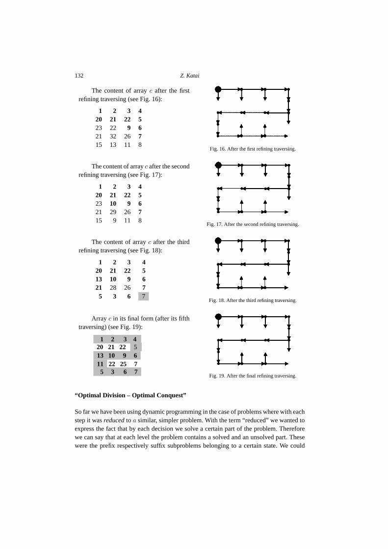
For a first go we fill up array c with the values given by traversing it row by row (fromtop to bottom, left to right). Of course we can take into consideration only neighboursc[i− 1][j] és c[i][j − 1] when filling element c[i][j] during the traversing (only these havealready been filled up), although on the optimal paths there are sections pointing to theleft, respectively upwards (short: backwards-edges), then elements c[i][j+1] és c[i+1][j]should essentially be taken into consideration. For example in the above presented prob-lem calculating the value c[3][3] assumes to know the value of c[3][4]. Furthermore wecan also say that after this filling up we get the shortest path only to those rooms , in caseof which they contain edges only pointing forwards (to the right, respectively down).What is the solution? We go again and again through array c, refining it. During thesefurther traversings we overwrite those array-elements to which there is a more advanta-geous path from a neighbouring element. This time we can take into consideration all fourdirections. When a new traversing does not bring any alterations, it means that we havereached the optimal solution. We can notice that there are as many refining traversings asthe number of backwards-edges in the subtree of the optimal paths. If we can still refineafter nm (number of the nodes of the contracted decision tree) traversings, it means thatin contradiction to the conditions of the problem, there is such an office-tour going roundwhich our money is becoming more

In what follows we are presenting the content of array c after the filling, respectivelyrefining traversings. We have written in bold those elements which already represent op-timal paths. In the attached pictures we wanted to show the way the subtree representingthe optimal solution is being built, in accordance to the principle of optimality from thebottom toward the top, from the simple toward the complex. In bold we have representedthe part of the tree which has already been built until the given step.

The content of array a in the problem:

1 1 1 119 19 19 1

3 1 3 1−2 19 19 1−6 −2 3 1

The content of array c after the fillingtraversing (see Fig. 15):

1 2 3 420 21 22 523 22 25 621 40 44 715 13 16 8

Fig. 15. After the filling traversing.

132 Z. Katai

The content of array c after the firstrefining traversing (see Fig. 16):

1 2 3 420 21 22 523 22 9 621 32 26 715 13 11 8

Fig. 16. After the first refining traversing.

The content of array c after the secondrefining traversing (see Fig. 17):

1 2 3 420 21 22 523 10 9 621 29 26 715 9 11 8

Fig. 17. After the second refining traversing.

The content of array c after the thirdrefining traversing (see Fig. 18):

1 2 3 420 21 22 513 10 9 621 28 26 7

5 3 6 7Fig. 18. After the third refining traversing.

Array c in its final form (after its fifthtraversing) (see Fig. 19):

1 2 3 420 21 22 513 10 9 611 22 25 75 3 6 7

Fig. 19. After the final refining traversing.

“Optimal Division – Optimal Conquest”

So far we have been using dynamic programming in the case of problems where with eachstep it was reduced to a similar, simpler problem. With the term “reduced” we wanted toexpress the fact that by each decision we solve a certain part of the problem. Thereforewe can say that at each level the problem contains a solved and an unsolved part. Thesewere the prefix respectively suffix subproblems belonging to a certain state. We could


say that as a result of the sequence of decisions D1, D2, . . . , Dn the problem was solvedstep by step. The question only was how to make these decisions, in order to get theoptimal solution. At a first glance these problems seem to be “greedy problems”, but asthe basic principle of the greedy selection is not applicable to them, “we have to” applythe dynamic programming.

An other field of the dynamic programming consists of problems which are closerto the “divide and conquer” technique. The essence of the “divide and conquer” is thatit divides the problem into two or more similar, simpler subproblems and builds up theoriginal problem’s solution from their solutions (of course the procedure is the same forthe subproblems, until we get trivial subproblems). What is the situation if the divisionof the problem into subproblems can be achieved in several ways? If this is the case,the question of the optimal division arises! In such situation the point is more than asimple “divide and conquer” problem. If at each step the optimal “cut” could be madewith a greedy decision, then we can say that the greedy technique facilitated the work ofthe “divide and conquer”. Should we not have enough information for the greedy cuts,but the principle of optimality is valid for the task of dividing the problem, dynamicprogramming might help the “divide and conquer” technique to find the optimal solution.

So we are speaking about a strategy which builds dynamic programming into the “di-vide” stage of the “divide and conquer” technique (this is called mixed method by TudorSorin, 1997). This means that the optimal sequence of decisions D1, D2, . . . , Dn char-acteristic for optimization problems basically means the optimally breaking down of theproblem into subproblems. By each decision the problem breaks down into similar, sim-pler subproblems ( in contradiction with the situation when it was reduced to one similar,simpler problem). When we say optimally division into subproblems, we consider that itis optimal because it involves the building of the optimal solution in the “conquer” stageof the “divide and conquer”. As the sequence of decisions D1, D2, . . . , Dn only meansthe way the problem optimally breaks into subproblems, in an intermediate Si stage (thatwe reached after a sequence of D1, D2, . . . , Di decisions) we cannot speak about a partof the problem which has already been solved (prefix subproblem). Therefore, in suchcase only the leaves-root oriented version of the dynamic programming can be taken intoconsideration. This is in accordance with the fact that the “divide and conquer” techniquesolves a father-subproblem only after having solved the son-subproblems (according tothe above introduced terminology by subproblems we mean suffix type subproblems).

The Principle of Optimality on a II Type Decision Tree

Let’s assume again that D1, D2, . . . , Dn is the sequence of decisions which optimallybreaks the problem up into subproblems. For simplicity we presume that the currentsubproblem falls into two further subproblems apart by each step ( until we get trivialsubproblems). How does the basic principle of optimality become evident in case of sucha problem? If we assume that after decision D1 the problem breaks up into two subprob-lems so that their further division is ensured by the subsequence of decisions D2, . . . , Dk

134 Z. Katai

respectively Dk+1, . . . , Dn, each of these should also be optimal (in the sense that theybreak up the corresponding subproblems in a way which leads to the optimal solution).

We could say that in so far as the sequence of decisions leading to the optimal so-lution is D1, D2, . . . , Dn, then the subsequence of decisions D2, . . . , Dk and Dk+1 forany k (k = 2, n − 1) is also optimal. Continuing this idea, it assumes that the couples ofsubsequence of decisions D3, . . . , Dk1 and Dk1+1, . . . , Dk, as well as Dk+2, . . . , Dk2

and Dk2+1, . . . , Dn for a certain k1 (k1 = 3, k − 1) respectively k2 (k2 = k + 2, n − 1)are also optimal. And so on . . . .

It is not difficult to realize that in so far as this situation occurs, the optimal so-lution of the general subproblem is represented by a section of sequence of decisionsDi, Di+1, . . . , Dj . What does it mean in this situation to build from down upwards? Wesolve the subproblems in the increasing order of the length of the sections of sequence ofdecisions representing their solution.

This situation is different from the one where by each decision the problem was re-duced to only one similar simpler subproblem and the validity of the basic principle ofoptimality was obvious. It might occur that the optimization of the subproblems we havebroken the problem up to, get into conflict.

Dynamic Programming on the II Type Decision Tree

We make this version of the dynamic programming easier to grasp through a solvedproblem.

Mirrorword: A string is given. Divide it into a minimal number of mirrorwords.

EXAMPLE. Be the string: ababb. We can see that it can be divided into mirrorwords inseveral ways:

(a) (b) (a) (b) (b), (a) (b) (a) (bb), (aba) (bb), (a) (bab) (b), (aba) (b) (b)The optimal solution is obviously represented by the third version.

The basic idea is that if the string is not a mirrorword itself, we cut it into two, thusbringing the problem back to the division into mirrorwords of two shorter strings. Havingdone this, the number of minimal mirrorwords of the original problem is given by theoptimal sum of the two parts. This sound like a “divide and conquer” algorithm. Butit is not only that, because the cuts can be performed in general in several ways andthere is no possibility to decide (with a greedy decision) which is the one leading to theoptimal solution. In the followings we are going to show the decision tree associatedto the problem, applied to the example. The nodes of the tree contain the starting andending indexes of the corresponding substring within the string. For example the node(1–5) represents the whole string (ababb), and (3–5) represents the substring abb.

The decision tree (see Fig. 20) differs from the usual because it presents the way theproblem can be broken up into its subproblems. For example the original problem canbe cut into two in four different ways: a|babb, ab|abb, aba|bb, abab|b. The optimal cut isthe third one, (which in this case also represents the solution), the one that leads to the


Fig. 20. The decision tree associated to mirrorword problem.

substrings (1–3) and (4–5), as these are already mirrorwords. We can notice that all theleaves of the tree – and only them – represent mirrorwords.

We can also read from the tree that the general form of the subproblems is: the optimaldivision of the substring (i − j) into mirrorwords. As in the general form there are twoindependent parameters and i � j, we are going to use the elements from the maindiagonal and above the main diagonal of a bidimensional array c[1..n][1..n] (n – thenumber of the characters of the string) to store the optimal values of the subproblems.The array-element c[i][j] will store the minimal number of mirrorwords corresponding tothe optimal division of segment (i − j).

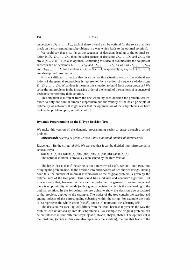
In accordance to what has been said before we can notice that if we overlap the iden-tical nodes of the decision tree, the nodes of the contacted decision tree thus obtained canbe rearranged so that they form a shape corresponding to a triangle above the main diag-onal of a n × n sized bidimensional array (the number of the nodes of the decision treewhich differ from each other is n(n+1)/2). This is noticeable in Fig. 21. The root of thetree gets into the nth position of the 1st row, in the same way as the optimal value of theoriginal problem will be stored in array c[1][n]. The strings containing one element areobviously mirrorwords, therefore the elements of the main diagonal store in any case theoptimal values of trivial subproblems, but of course there can be other array-elements thesubproblems corresponding to them also being trivial in case the respective substring isa mirrorword itself. Every mirrorword-substring is represented by leaves in the decisiontree and in the contracted tree as well.

136 Z. Katai

Fig. 21. The contracted decision tree attached to mirrorword problem.

The Check of the Basic Principle of Optimality

As the two subproblems created after a certain cut are independent from each other, andthus their optimal solution cannot get in conflict, the basic principle of optimality ob-viously applies here. Namely: If the segment (i − j) is divided after the first optimaldivision into the pair (i− k) and (k + 1, j) then their further cutting through the optimaldivision is certainly optimal concerning them, too. Since had one of them a better divi-sion than the one through which it is divided by the optimal division of the segment (i, j),then choosing this one we would get to a better division for segment (i, j), too. But thiscontradicts the condition that we started from the optimal division of segment (i − j).Therefore the division of the original string can be determined from the optimal divisionof the substrings.

The Principle of Optimality in the “Contracted Decision Tree”

Heading from the leaves to the root we leave on each fathernode that couple of sonnodes,whose corresponding couple of subproblems have the minimal total value of optimums(we prune the rest from the tree). We have represented the optimal choices on the con-tracted tree in bold.


The Principle of Optimality in the Array Storing the Optimal Values

We fill the elements from the main diagonal, respectively from above the main diagonalof array c according to the following recursive formula:

c[i][j] =

⎧⎪⎨⎪⎩

1, if the string-segment (i − j)is a mirrorword,

mini�k<j

{c[i][k] + c[k + 1][j]}, in the opposite case.

As this formula is suggesting, the elements should be filled up in such an order, that whenthe filling up of element c[i][j] is to follow, the couples of elements c[i][k] and c[k +1][j](i � k < j) should be already filled up. Such an order is possible if starting from theelements next to the main diagonal, we advance from diagonal to diagonal until elementc[1][n].

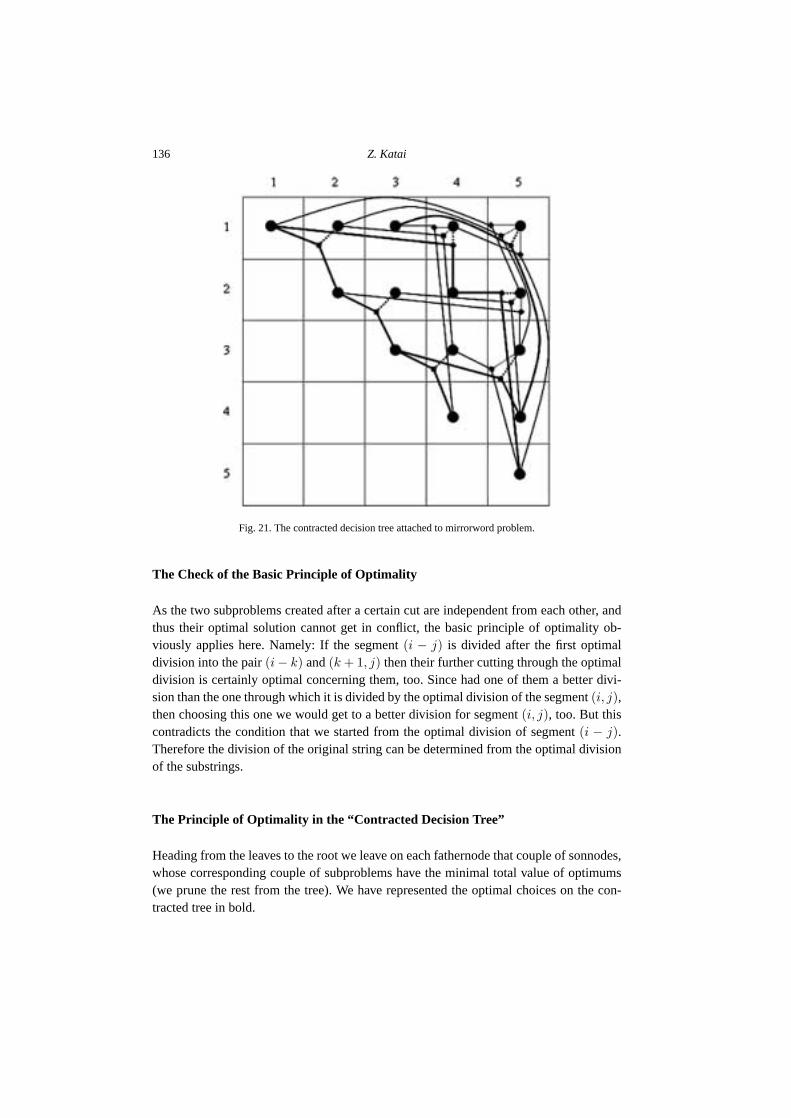
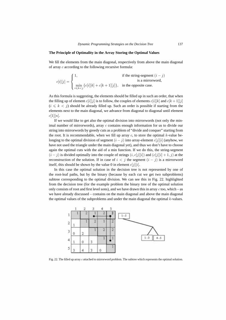
If we would like to get also the optimal division into mirrorwords (not only the min-imal number of mirrorwords), array c contains enough information for us to divide ourstring into mirrorwords by greedy cuts as a problem of “divide and conquer” starting fromthe root. It is recommendable, when we fill up array c, to store the optimal k-value be-longing to the optimal division of segment (i− j) into array-element c[j][i] (anyhow, wehave not used the triangle under the main diagonal yet), and thus we don’t have to chooseagain the optimal cuts with the aid of a min function. If we do this, the string-segment(i− j) is divided optimally into the couple of strings (i, c[j][i]) and (c[j][i] + 1, j) at thereconstruction of the solution. If in case of i < j the segment (i − j) is a mirrorworditself, this should be shown by the value 0 in element c[j][i].

In this case the optimal solution in the decision tree is not represented by one ofthe root-leaf paths, but by the binary (because by each cut we get two subproblems)subtree corresponding to the optimal division. We can see this in Fig. 22. highlightedfrom the decision tree (for the example problem the binary tree of the optimal solutiononly consists of root and first level sons), and we have drawn this in array c too, which – aswe have already discussed – contains on the main diagonal and above the main diagonalthe optimal values of the subproblems and under the main diagonal the optimal k-values.

Fig. 22. The filled up array c attached to mirrorword problem. The subtree which represents the optimal solution.

138 Z. Katai

Conclusions

The strength of the above presented approach is its illustrability. This is extremely im-portant in teaching dynamic programming. But this is something more than a didacticpoint of view. This illustrative approach can be very useful in understanding the dynamicprogramming as a method and in the classification of its different versions (I and II typedecision trees).

The terminology used is also very illustrative: contracted decision tree, prefix andsuffix subproblems, root-leaves, respectively leaves-root oriented dynamic programming,“optimal division – optimal conquest”.

Of course there is no question of having completely exhausted the analysis of thetopic of dynamic programming from this point of view. We meant this paper to be anintroduction, leaving space for more studies.

References

Andone, R., and I. Garbacea (1995). Fundamental Algorithms a C++ Perspective. Libris Press, Cluj-Napoca(in Romanian).

Cormen, T.H., C.E. Leirserson and R.L. Rives (1990). Introduction to Algorithms. The Massachusetts Instituteof Technology.

Kátai, Z. (2005). “Upperview” algorithm design in teaching computer science in high schools. In TeachingMathematics and Computer Science. University of Debrecen, Hungary, pp. 222–240.

Tudor, S. (1997). Programming Techniques. L&S InfoMat Press, Bucuresti (in Romanian).

Z. Katai is an assistant professor at Sapientia-Hungarian University of Transylvania.He is going to obtain the PhD degree on February 15, 2007. His reasearch interests areteaching methods (especially in informatics), dynamic programming, the role of sensesin teaching-learning process.

Dinaminio programavimo strategijos, sprendžiant optimizavimouždavinius, remiantis medžio algoritmu

Zoltan KATAI

Straipsnio tikslas – pristatyti patikrintas dinaminio programavimo strategij ↪u charakteristikas,remiantis medžio algoritmu ir pasiulyti aiški ↪a priemon ↪e t ↪u strategij ↪u analizei ir klasifikacijai,padedanciai perprasti šios programavimo technologijos esm ↪e.

Documents

Dynamic Programming Strategies on the Decision Tree … · a clear tool for their study and classiﬁcation which can help in the comprehension of the essence of this programming