DYNAMIC RESPONSE OF MINI CANTILEVER BEAMS IN VISCOUS MEDIA

by

Anamika Sharmin Mishty

A thesis submitted in partial fulfillment of the requirements for the degree

of

Master of Science

in

Mechanical Engineering

MONTANA STATE UNIVERSITY Bozeman, Montana

November 2010

©COPYRIGHT

by

Anamika Sharmin Mishty

2010

All Rights Reserved

ii

APPROVAL

of a thesis submitted by

Anamika Sharmin Mishty

This thesis has been read by each member of the thesis committee and has been found to be satisfactory regarding content, English usage, format, citation, bibliographic style, and consistency and is ready for submission to the Division of Graduate Education.

Dr. Ahsan Mian

Approved for the Department of Mechanical & Industrial Engineering

Dr. Christopher H.M. Jenkins

Approved for the Division of Graduate Education

Dr. Carl A. Fox, Vice Provost

iii

STATEMENT OF PERMISSION TO USE

In presenting this thesis in partial fulfillment of the requirements for a master’s

degree at Montana State University, I agree that the Library shall make it available to

borrowers under rules of the Library.

If I have indicated my intention to copyright this thesis by including a copyright

notice page, copying is allowable only for scholarly purposes, consistent with “fair use”

as prescribed in the U.S. Copyright Law. Requests for permission for extended quotation

from or reproduction of this thesis in whole or in parts may be granted only by the

copyright holder.

Anamika Sharmin Mishty November 2010

iv

ACKNOWLEDGEMENTS

I would like to acknowledge and thank all who participated in the work which has

culminated in this report. First my thanks to Mechanical Engineering Department and Dr.

Ahsan Mian for his expertise and guide throughout this thesis. My Thanks to Center for

Biofilm Engineering and Dr. Phil Stewart who provided the partial funding for the

research. My thanks to Dr. Christopher H. M. Jenkins for his help by providing vibro-

thermography equipments for the thesis. Thanks to Dr. David Miller and Dr. Brock J.

Lameres who gave their wise advice for the thesis. My special Thanks to Dr N.M. Awlad

Hossain of Eastern Washington University for his valuable advice to my work. And

finally to all Faculty members, who have given their moral support to complete this

thesis.

v

TABLE OF CONTENTS

1. INTRODUCTION .......................................................................................................... 1 2. BACKGROUND ............................................................................................................ 7 3. EXPERIMENTAL SETUP........................................................................................... 15

Apparatus ...................................................................................................................... 15

Polytec Laser Scanning Vibrometer ......................................................................... 16 Shaker for the Excitation of the Beam:..................................................................... 20 Stainless Steel Beam................................................................................................. 21 Mass of Aluminum ................................................................................................... 22 Plastic Cup for the Liquid ......................................................................................... 23 Aluminum Holder ..................................................................................................... 23 Materials used for Tests ............................................................................................ 23 Experimental Setup for Configuration A.................................................................. 23 Experimental Setup for Configuration B .................................................................. 24

4. RESULTS AND DISCUSSION................................................................................... 27

Configuration A ............................................................................................................ 27 Configuration B ............................................................................................................ 30

Standard Deviation of the Result .............................................................................. 33 Basic Examples......................................................................................................... 34 Mathematical Solution of the Frequency in Air (Configuration A) ......................................................................... 35 Mathematical Solution of the Frequency in Air (Configuration B) ......................................................................... 36

5. FINITE ELEMENT ANALYSIS ................................................................................. 38

Procedure .................................................................................................................. 40 Plane 42..................................................................................................................... 41

Element Description.............................................................................................. 41 Input Data.............................................................................................................. 41

Output Data................................................................................................................... 43 FLUID79 (2-D Contained Fluid) .............................................................................. 44

Element Description.............................................................................................. 44 FLUID79 Input Data............................................................................................. 44 FLUID79 Output Data .......................................................................................... 45

FLUID79 Assumptions and Restrictions ...................................................................... 45

vi

TABLE OF CONTENTS - CONTINUED

FLUID 29.................................................................................................................. 46 Element Description.............................................................................................. 46 FLUID29 Input Data............................................................................................. 47 FLUID29 Output Data .......................................................................................... 49

Results of Analysis ................................................................................................... 52 Harmonic Solution.................................................................................................... 55

6. MEMS DESIGN AND STEPS OF FABRICATION................................................... 57

Material Deposition ...................................................................................................... 58

Magnetron Sputtering System................................................................................... 58 Manual Spin Coater .................................................................................................. 59 Photolithography....................................................................................................... 59

Contact Aligner..................................................................................................... 59 Programmable Spin Coater ................................................................................... 59

Material Etching........................................................................................................ 60 Plasma Etcher........................................................................................................ 60 Wet Benches ......................................................................................................... 60

Characterization ........................................................................................................ 60 Packaging.................................................................................................................. 61 Fabrication Sequences .............................................................................................. 61

7. FUTURE WORK AND CONCLUSION ..................................................................... 65 REFERENCES ................................................................................................................. 66

APPENDIX A: Ansys Program.................................................................................... 69

vii

LIST OF TABLES

Table Page

1: Fluid rheological properties and measured natural frequencies, band width, quality factors and inverse quality factors configuration A)...............28 2: Fluid rheological properties and measured natural frequencies, band width, quality factors and inverse quality factors (configuration B). .............30 3: Comparison between the results of configuration A and B. ....................................33 4: Data for standard deviation for configuration A......................................................34

5: Data for standard deviation for configuration B......................................................35

6: Experimental modal response of cantilever beam. ..................................................53 7: Effect of changing Viscosity without changing Bulk Modules...............................53

8: The increment of frequency with increment of Density. .........................................54

9: Comparison of the result of harmonic analysis with the actual result. ....................56

viii

LIST OF FIGURES Figure Page

1: End mass oscillates in viscous fluid (Configuration A). .........................................15

2: Beam end oscillates in viscous fluid (Configuration B). .........................................15

3: Polytec laser scanning vibrometer with control unit and display. ...........................17

4: Laser head scanning device with 3D movement controller. ....................................18 5: Control Unit and data acquisition platform of Doppler vibrometer. .......................18

6: Vibration display unit. .............................................................................................19 7: The power amplifier for create vibration.................................................................20 8: Shaker with connecting cord of amplifier and beam holder. ...................................21

9: The T shaped Aluminum mass of configuration A.................................................22 10: Beam without mass in the vertical arrangement. ...................................................25

11: Frequency response curve in different fluid media (Configuration A). ................28 12: Resonant Frequency variation with viscosity (Configuration A). .........................29 13: Quality factor (Q) variation with viscosity (Configuration A). .............................29

14: 1st and 2nd Frequency response curves in different fluid media (Configuration B)...................................................................................................31 15: 1st Frequency response curve in different fluid media (Configuration B). ............31 16: Resonant Frequency variation with viscosity (Configuration B). .........................32 17: Quality factor (Q) variation with viscosity (Configuration B). .............................32 18: Dimensions of the beam with load ( configuration A). .........................................36

19: Dimensions of the beam with load (configuration B)............................................37

ix

LIST OF FIGURES – CONTINUED

Figure .............................................................................................................................Page 20: Experimental setup to predict modal response of cantilever beam. ......................40 21: PLANE42 Geometry..............................................................................................41

22: PLANE 42 stress output. .......................................................................................43

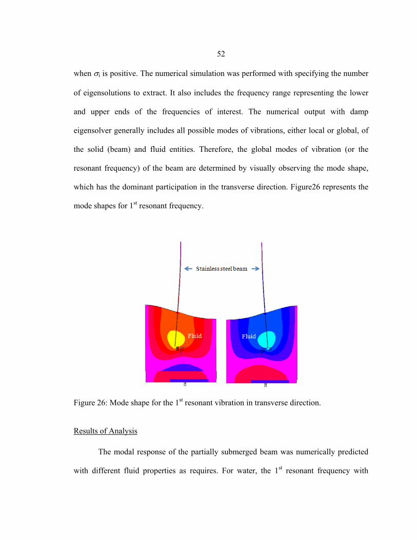
23: Fluid79 Geometry. .................................................................................................44 24: FLUID29 Geometry...............................................................................................47 25: FE model of cantilever beam partially submerged under fluid. ............................50 26: Mode shape for the 1st resonant vibration in transverse direction. ........................52

27: Increase of frequency by the decrease of density of viscous fluids.......................55 28: Result found by harmonic solution for water. .......................................................56 29: The top view of the beam with piezo resistor........................................................64

x

ABSTRACT

In concurrent engineering, viscosity and density of a fluid are two important parameters as they are the indicators of some predefined standards of the concerned fluids in some specified application. Arguably fluids play an important role in all major engineering applications starting from automobile to biofilm. In this work, we will demonstrate the use of mini cantilever beams for characterization of rheological properties of viscous materials such as lubricating oils. Further miniaturization of the test platform can lead to a MEMS device that can potentially be used for measuring the rheological properties of soft viscoelastic materials such as biofilm. Miniaturization of the measuring instrument is necessary so a small sample volume can be used to perform the test. In this study, the dynamic response of cantilever beams was measured experimentally in air and viscous fluids (e.g. water, and lube oils of three different grades) using a duel channel PolyTec scanning vibrometer. The changes in dynamic response of the beam such as resonant frequency, frequency amplitude, and the Q-factor were compared as functions of the rheological properties (density and viscosity) of fluid media. It may be mentioned here that we used two cantilever beam configurations, one was the plain small stainless steel beam and another was a small stainless steel beam with an aluminum mass attached to it. For both the configurations, the samples were excited by an external shaker at sweeping frequency modes and the beams’ motions were recorded by the laser vibrometer focused at different locations of a beam’s surface. The reflected signal is directed to a split photo detector whose output is sent to fast-Fourier Transform [FFT] spectrum analyzer.

1

CHAPTER 1

INTRODUCTION

Viscosity and density of a fluid are two important parameters as they are the

indicators of some predefined standards of the concerned fluids in some specified

application. Arguably fluids play an important role in all major engineering applications

starting from automobile to biofilm. Viscosity is often thought as the fluid’s friction,

resistance to flow or the fluid’s resistance to shear when the fluid is in motion [1]. The

viscosity of a fluid is often represented as a coefficient that describes the diffusion of

momentum in the liquid. The measurement of viscosity has been employed for many

decades to monitor and test lubricants, blood, mucus, adhesives, paint, fuels and other

fluids. Therefore keeping track of the dynamical behavior of these fluids (i.e., rheology)

is necessary as they undergo temporal changes.

In all engineering processes we use different types of fluids. There are fuels for

the combustion in power generation, fluids for lubrication, fluids for cooling etc.

Depending upon the types of applications these fluids vary in density and viscosity,

processes in refineries these fluids are designated with standard names (e.g. SAE 70) that

describes the properties of that fluid. The initial measurements are thus performed at the

corresponding plants. But is also important to keep track of these properties so that we

can replace them if any degradation occurs and thus maintain smooth operation of the

engineering process.

2

Rheology is a more complex study of the flow of matter; mainly liquids, but also

soft solids, gels, pastes and even solid materials that exhibit some level of flow (i.e., do

not just deform elastically). Rheology applies to substances that have a complex

structure, including: mud, sludge, suspensions, polymers, petrochemicals and biological

materials. The flow of these complex materials cannot be characterized by a single value

of viscosity, instead viscosity changes with changing conditions. For example: ketchup's

viscosity lowers when it is shaken, corn flour’s viscosity increases when it is struck.

Encompassing a number of various methods with vastly different guiding

principles, the field of micro rheology has developed a significant growth in last couple

of years. The shear rate of dependent properties of fluid are typically quantified by

oscillatory measurements.[11] In this type of oscillatory measurement the material is

placed in forced harmonic oscillation where its stress and strain vary harmonically. From

the stimulus and response, the elastic properties can be derived. The common

methodologies used in the measurement of micro mechanical properties are magnetic

tweezers, passive particle trapping, optical tweezers, falling ball and atomic force

microscopy or AFM.

The magnetic tweezers consists of adhering ferromagnetic beads [11] to the

surface of biological cells, rotating them in a constant magnetic field and measuring their

response. The passive particle tracking involves tracking the thermal motion of injected

micron sized particles in a cell. The optical tweezers involve trapping a particle in an

optical trap, vibrating the trap, and measuring the beads response by scattering. The

AFM[11] methods involve using a converted atomic force microscope (AFM) probe of

3

known stiffness to excite the cell and then measure its displacement using a laser

reflected off the surface of the AFM tip to a photo sensitive detector.

In practice, rheology is concerned with materials whose properties are between

purely elastic material and Newtonian fluids, where mechanical behavior cannot be

described by classic theories. A frequent reason for the measurement of rheological

properties can be [12] found in the area of quality control, where raw materials must be

consistent from batch to batch. For this purpose, flow behavior is an indirect measure of

product consistency and quality.

Another reason for studying flow behavior is that a direct assessment of

processibility can be obtained. For example, a high viscosity liquid requires more power

to pump than a low viscosity one. Knowing its rheological behavior, therefore, is useful

when designing pumping and piping systems.

It has been suggested that rheology is the most sensitive method for material

characterization because flow behavior is responsive to properties such as molecular

weight and molecular weight distribution. This relationship is useful in polymer [12]

synthesis, for example, because it allows relative differences to be seen without making

molecular weight measurements. Rheological measurements are also useful in following

the course of a chemical reaction. Such measurements can be employed as a quality

check during production or to monitor and/or control a process. Rheological

measurements allow the study of chemical, mechanical, and thermal treatments, the

effects of additives, or the course of a curing reaction. They are also a way to predict and

control a host of product properties, end use performance and material behavior.

4

At present, there is a growing interest in the mechanical properties of biofilms that

appear to exhibit the behavior of rheological fluids. The understanding of these properties

provides the necessary foundation for effective biofilm control in industrial and medical

environments. In particular, important applications of biofilm rheology concern

detachment processes and frictional energy losses in transport pipelines. Similarly, of

[10]critical importance is the problem of biofilm detachment in food production facilities

and drinking water systems, which may result in the potential transmission of pathogens.

In the field of biofilm and petroleum engineering the measurement of fluid

viscosity is a particularly demanding problem when precision is required. For many

engineering application we use a comparative test as a quicker and generally a more

convenient alternative. Often these viscosity measurement techniques require both large

experimental apparatus and large sample volume. Here we use the Polytec He-Ni Laser

vibrometer for measuring viscous properties of fluids utilizing force cantilever, driven by

the external shaker, need relatively small sample. Lot of works have developed results for

the dynamics of scanning probe force beams, focus on the interaction of the probe tip

against a sample surface.

With the advancement of Laser, there have been many devices studied, developed

and fabricated to characterize the mechanical properties of viscous liquids. Here we

introduce a flexible device for characterization of rheological properties of viscous

liquids which will tends to apply to measure the viscosity soft viscoelastice material like

biofilm where miniaturizing the measuring instrument and reducing the volume of liquid

or soft solid required for testing are of great interest. In this device little amount of liquid

5

will be placed on the small cantilever beam and vibration in sonic velocity will be

imposed on it that is in contact with the specimen in resonance frequency. The dynamic

response of the cantilever would be investigated experimentally in the air and the viscous

liquids with varying viscosity. With the increase of viscous damping coefficient the Q-

factor decreases with the fixed dynamic gap. The vibration resulting from the applied

stress is quantified by measuring the cantilever deflection with a duel channel scanning

vibrometer. The deflection is governed by the viscoelastic properties of the cantilever

beam and of the test specimen. The relative analysis of the result from the cantilever and

the test material to the measured deformation are quantified by comparing a previously

calibrated result and on the process to compare with an independent modeling and

numerical analysis. The result from this rheometer used to characterize the liquids is in

good agreement with the results of conventional mechanical rheometry.

Here we investigated the response of small stainless steel beam with the

aluminum mass attached on its tip ,driven vertically by the external shaker, were recorded

into account through both a velocity dependent damping / sweeping / periodic chirp

frequency as well as induced mass submerged in the fluid being carried along with the

cantilever beam. The beam’s motion was recorded by a focused laser beam positioned on

the different position of cantilever with the reflected signal directed to a split photo

detector whose output is sent to fast-Fourier Transform [FFT] spectrum analyzer.

Data were /recorded by monitoring the 1st peak response frequency of the lever in

the air and then in other liquids. After taking several sets of data for one liquid the beam

have rinsed to minimize contamination. The time taking for taking a set of data depends

6

on the FFT lines and the type of the frequency we want, but as usually maximum limit is

1 minute. Driven resonance characterization was done in the ambient temperature and in

the air and the dimensions of the beam, level of the submerged part of the beam or the

mass were fixed. Experimental was compared with the theoretical results in the air. From

the data taken we find out the peak frequency and quality factor of the cantilever.

Immersions in liquid result in even greater changes to the frequency responses

with resonant frequencies quality factors being an order of magnitude smaller than their

corresponding values in air. They have some assumptions here for taking data like the

fluids we use are incompressible in nature, beam has a uniform cross section over its

entire length and the length is much bigger than width and thickness. The amplitude of

the vibration was limited within the range of vibrometer tolerance limit.

7

CHAPTER 2

BACKGROUND

In various fields of engineering, the measurement of fluid viscosity and density is

a particularly demanding problem when precision is required. For many engineering

applications, different types of rheometers are used [1]. Often these viscosity

measurement techniques require both large experimental apparatus and large sample

volume. In this study, we explore the use of small stainless steel cantilevers of two

configurations for rheological measurement purposes. Results obtained from this

preliminary study will be used to design flexible MEMS (micro-electromechancial

systems) devices for characterizing rheological properties of soft viscoelastic materials

such as biofilm. In this particular application, miniaturizing the measuring instrument is

necessary due to the presence of microscale heterogeneity in the mechanical/rheological

properties.

In addition, occasionally the available volume of the liquid of interest may be

sufficiently small where the conventional methods of rheometry such as cone and plate

rheometry [2], stormer viscometry [2] or falling ball viscometry [2] are inappropriate.

Consequently, there is a growing interest in the use of MEMS devices to measure the

required properties, especially with an aim of encouraging high throughput. These

devices include pressure sensors [2], optical tweezers [2] and micro-particle image

velocimetry [2], and others.

8

The conventional laboratory equipment is often not applicable due to its cost, and

other precondition such as vibration free mounting and overall space requirements and

volume. On the other hand taking the sample for such devices often involves manual

labor, tending to be time consuming and error-prone. The required volume for the

rheological characterization of fluids can be minimized by using micromechanical

cantilevers as viscosity sensor [1].

For sensing viscosity and density some important work done on microacoustic

sensors such as quartz crystal resonators or SAW devices have proved particularly useful.

In the field microacoustic sensors such as quartz thickness shear mode [TSM] resonators

[11] and surface acoustic wave [SAW] devices, for example, have proved particularly

useful alternatives with respect to traditional viscometer. These devices can measure

viscosity at comparatively high-shear rates and small vibration amplitudes. The results

for non-Newtonian liquids are not directly comparable to these obtained from

conventional viscometers. But those microacoustic devices may not be sufficient to detect

rheological effects for complex liquid such as emulsions which are present only

macroscopic scale. The vibrating structures usually feature lower resonance frequencies

and higher vibration amplitudes, making them more suitable for non-Newtonian and

complex liquids. In this case Microcantilevers have been successfully used for

simultaneous measurement of liquid’s viscosity and mass density requiring less sample

volume. On the other hand a highly sensitive optical readout is required to determine the

beam’s vibration amplitudes. When the cantilevers are immersed in liquid, they face

strong deterioration of the quality factor due to high dissipative effects. Gradually the

9

vibration amplitudes drops even more, limiting the sensor’s measurement range to low

viscous liquids. So the doubly clamped micromachined cantilevers are used that are

driven by Lorentz forces or by the piezoelectric effect have been utilized as liquid

property sensors. Feasibility of these sensors has been demonstrated for viscosities in the

range up to several Pa.s. In this set up the cantilevers feature piezoelectric excitation as

well as piezoelectric readout. The vibrating part is longer but since only the cantilever tip

is immersed in the liquid, the induced damping of the cantilever vibration is kept low.

The high quality factors ranging from 20-60 even for highly viscous liquids have been

shown by the sensors. The detection of the of the resonances could be accomplished by a

simply readout electronics and the measurement range is greatly extended but hand

sensitivity is decreased on the other sensor principle allows attaching different tips of

well-defined geometries to the cantilevers with PZT bending actuator. However this type

of set up do not show a simple relationship between the result of such a measurement and

the liquid parameters.

Another research group has done a set of experiment by a simple measurement

tool, where the sensor consists of a micromechanical cantilever used as in an atomic force

microscopy which is integrated into a closed fluid handling system [12]. From the

analysis of the power spectral density of the fluctuations of the cantilever deflection

signal fluid properties are derived. Here they used the standard consumer computer

components, which limit the costs for the hard ware. The measured viscosity could be

evaluated with an error smaller than 5%. This measurement system use the video camera,

attached on the top plate of the frame for optical control and can be adjusted in the z-

10

direction for focusing pre-amplifier, a signal conditioning electronics and a commercially

available sound card for analog to digital conversation. The support for the measuring

chamber was placed at the bottom of the frame which can be moved in x and y directions

to adjust the cantilever. The liquid was fed to the measurement chamber by a syringe

pump. For all measurements commercial cantilevers were used like NSC12,

MikroMasch, Tallinn, Estinia. In this set up they use E-type cantilevers with a nominal

resonant frequency of 29 kHz were used for no flow measurements. E type lever and

additionally a harder cantilever like D-type, whose nominal resonant frequency 39 kHz.

The cantilever deflection was read by light lever detection. The laser diode and the photo

split detector are set up in a way that this mounting allows the operator to place the spot

of the laser beam in the center of the diode. To evaluate the absorption of light in the

liquid in the vicinity of laser wavelength, absorption spectra were acquired using a UV-

VIS spectrometer [ISS UV-VIS USB 4000, ocean optics, Dunedin, FL, USA] that was

equipped with a grating and a diode array for simultaneous acquisition of full spectra

within a range from 200nm to 950 nm. The test was done on air water and sugar

solutions. Here is a systematic discrepancy between theoretically predicted and

experimentally measured Q factors. Such a deviation could be a sign of heating up of the

solutions by laser during the measurement process since viscosities are reduced at higher

temperature.

The other research [15] group proposed the technique which overcomes the

restrictions of previous measurements that used microcantilevers, which are limited to

liquid viscosity only, and require independent measurement of the liquid density. The

11

technique presented there only requires knowledge of the cantilever geometry, its

resonant frequency in vacuum and its linear mass density. Here the use of microcantilever

in rheological measurements of gases and liquids is demonstrated. The viscosity and

density of both gas and liquid, which can range over several orders of magnitude, are

measured simultaneously using a single microcantilever. The microcantilever technique

probes only minute volumes of fluid [<1nL], and enables in situ and rapid rheological

measurements. This is an indirect contrast to establish some methods, such as ‘cone and

plate ‘method and Coquette’ rheometry which are restricted to measurements of liquid

viscosity, require large sample volumes, and are incapable of in situ measurements. They

also described a simple but robust calibration procedure to determine the latter two

parameters, from a single measurement of the resonant frequency and quality factor of

the cantilever in a reference fluid (like air) if these are unknown. By measuring the

frequency response of a microcantilever immersed in the fluid, information regarding the

rheological properties of the fluid, in principle, can be determined. The application is

predicted on the frequency response of the microcantilever is sensitive to the rheological

properties of the fluid consideration. The frequency responses of cantilevers of

macroscopic size like 1 meter are insensitive to the viscosities of the fluids in which they

are immersed. In contrast for AFM microcantilevers, which are approximately 100micron

in length, fluid viscosity can significantly affect their frequency response. This property

has permitted the use of microcantilevers as small scale viscometer. In previous

rheological application of microcantilevers is restricted to measurement of liquid

viscosity only with density and the properties of gases being outside the realm of its

12

applicability. With that a priori and independent measurement or knowledge of the liquid

density is required, which intern further restricts the utility of the microcantilever

technique. In this research they also demonstrated for the first time that the frequency

response of microcantilevers can be used to measure the density and viscosity of both

gases and liquids. This is achieved by using the theoretical model of Sader [1998] for the

frequency response of AFM cantilevers immersed in viscous fluids. They emphasized

that, unlike previous works that use microcantilevers, this application is not restricted to

the viscosity of the liquids and does not required a priori knowledge of the density of

fluid. By using a single microcantilever, the density and viscosity of both gases and

liquids are measured simultaneously. In their model the microcantilever is assumed to

have a uniform cross section over its entire length, and its length is much bigger than its

width. For a cantilever beam of rectangular cross section, it is also assumed that the width

greatly exceeds the thickness of the cantilever. These assumptions are satisfied by many

microcantilevers found in practice. They established that the frequency response of a

cantilever beam is well approximated by that of a simple harmonic oscillator, when the

quality factor Q greatly exceeds unity. All their measurements were performed using the

AFM, and the deflections of the microcantilevers were measured using the optical

deflection technique. A detection system was needed to monitor the frequency response

of the microcantilevers in fluid. The modification also possible if this would also allow

the microcantilever could be actively excited to eliminate any signal to noise problems, as

would be the case in monitoring the thermal noise spectrum. This model used to extract

the fluid density and viscosity from the measured frequency response requires the quality

13

factor Q>1. If this is not the case, then the analogy with the response of a simple

harmonic oscillator is not valid. They found that for fluid and cantilever combinations

where heavy damping is present (Q<1), it is impossible to fit the measured spectra to the

response of a simple harmonic oscillator. However that didn’t place a fundamental

restriction on the method, since by using different cantilever in the same fluid a different

quality factor is obtained. Provided this quality factor is larger than unity, the

methodology presented here is applicable. Consequently, to fully utilize the capabilities

of the microcantilever technique, it is suggested to use a range of different cantilevers,

preferably in a cantilever array configuration. This would enable fluids with a wider

range of properties to be measured than those accessible using a single microcantilever,

as demonstrated. The corresponding measurements have good agreement between the

microcantilever results and the published literature values with errors of less than 14% in

all cases. These errors are consistent with the errors in the theoretical model for the

frequency response, which were found to be less than approximately 10%.

In all the studies explained before, the researchers have performed limited

theoretical calculation in addition to the experimental measurements. However, the use of

very popular and effective finite element modeling scheme is not adopted to optimize the

experiment design. In this study, we first calculate the resonance frequency of the

cantilever beams (two different beam configurations such as a beam with or without mass

added with it) in air by the using conventional beam theorems. Next, we measured the

resonant frequencies of the same beams in air using the vibrometer and compared the

result in air to match the consistency of the experimental result in air with theoretical one.

14

Once the test is calibrated well, we repeated the resonant frequency measurements by

submerging the beam tip or mass in different viscous liquids such as water, and DTE

lubricating oils of three different grades. Finally, one beam configuration was modeled

using the finite element analysis software ANSYS and compared the experimental results

with the finite element analysis results. First, two-dimensional finite element analysis

(FEA) was performed for the beam partially submerged in water and FEA results are

compared with the experimental findings to validate the FEA modeling scheme. Here we

performed both harmonic and modal analysis. From modal analysis, when the FEA

results are within 5% of the experimental measurements, it can be assumed that the

model is acceptable. Finally, process steps for fabrication of the MEMS micro-cantilever

beams are presented so that the next generation graduate students can receive some

guidelines for the continuation of the work.

15

CHAPTER 3

EXPERIMENTAL SETUP

Apparatus

For this experiment, we used two configurations, A (Figure 1) and B (Figure 2).

Viscous media

PolytecVibrometer

Base vibrations at 

sweeping frequencies. Stainless steel 

beam Aluminum mass

Figure 1: End mass oscillates in viscous fluid (Configuration A).

Viscous media

Polytec Vibrometer

Stainless steel beam

Base vibrations at 

sweeping frequencies.

Figure 2: Beam end oscillates in viscous fluid (Configuration B).

16

And each of these instruments of these apparatus are described below:

Apparatus consists of:

a. A Polytec Laser Scanning Vibrometer

b. A shaker for the excitation of the beam

c. A stainless steel beam.

d. A ‘T’ shaped mass of aluminum attached on the beam.

e. A plastic cup for the liquid.

f. An aluminum holder to hold the beam.

g. Liquids of several types.

Polytec Laser Scanning Vibrometer

Polytec Scanning Vibrometer measures(16) the two-dimensional distribution of

vibrations. Polytec offers a comprehensive line of scanning laser Doppler vibrometers

(SLDV). Scanning offers all the advantages of a laser vibrometer together with speed

ease of use, laser positioning accuracy and comprehensive data processing in a single

automated, turnkey package.

Users get a very quick, easily understood and accurate visualization of a

structure's vibration characteristics without the inconvenience of attaching and

interpreting data from an array of transducers. An SLDV includes one or three compact

scan heads, data management system and powerful software for control of the scanners,

data processing and display. Here we used the PSV-400 Scanning Vibrometer. The PSV-

400 Scanning Vibrometer provides cutting edge measurement technology for the analysis

and visualization of structural vibrations. Entire surfaces can be rapidly scanned and

17

automatically probed with flexible and interactively created measurement grids, zero

mass loading and no time-consuming transducer mounting, wiring and signal

conditioning. The PSV-400(fig3) offers technical excellence, ease of use and features,

designed for resolving noise and vibration issues in the automotive, aerospace, data

storage, micro systems, commercial manufacturing and R&D markets.

Figure 3: Polytec laser scanning vibrometer with control unit and display. The PSV-400 is easy and intuitive to operate, especially when compared with traditional

multipoint vibration measurement methods requiring time-consuming preparation of the

test object and sensors. To setup the system, we have to define the geometry and scan

grid, and measure. The vibrometer automatically moves to each point on the scan grid,

18

measures the response and validates the measurement by checking the signal-to-noise.

When the scan is complete, choose the appropriate frequencies and then display and

animate the deflection shape in several convenient 2-D and 3-D presentation modes.

These on-screen (fig6) displays are extremely effective tools for understanding the details

of the structural vibration.

Figure 4: Laser head scanning device with 3D movement controller.

Figure 5: Control Unit and data acquisition platform of Doppler vibrometer.

19

At the heart of every Polytec PSV-400 system is the laser Doppler vibrometer – a very

precise optical transducer used for determining the vibration velocity and displacement at

a point by sensing(fig6) the frequency shift of back scattered light from a moving surface.

Figure 6: Vibration display unit.

The PSV-400 Scanning Vibrometer is a powerful data acquisition platform that

can seamlessly integrate into the engineering workflow and the IT environment. The

system provides input interfaces for geometry data from CAE and FEM packages or from

the convenient Geometry Scan Unit. All measurement results are available to third party

applications through various export filters and Poly File Access, an open data interface. A

powerful post processor is integrated in the PSV Software to apply various mathematical

operations to the measured data. External software packages can control the PSV

remotely by using an integrated Visual Basic® compatible scripting engine. The PSV-

400 Scanning Vibrometer is used to study objects of very different sizes including large

20

automobile bodies, airplane fuselages, ship engines and buildings as well as tiny silicon

micromachines, hard disk drive components and wire bonders. Demanding applications

such as measurements on hot running exhausts, rotating surfaces, underwater objects,

delicate structures or ultrasonic devices are all made possible by the PSV-400.

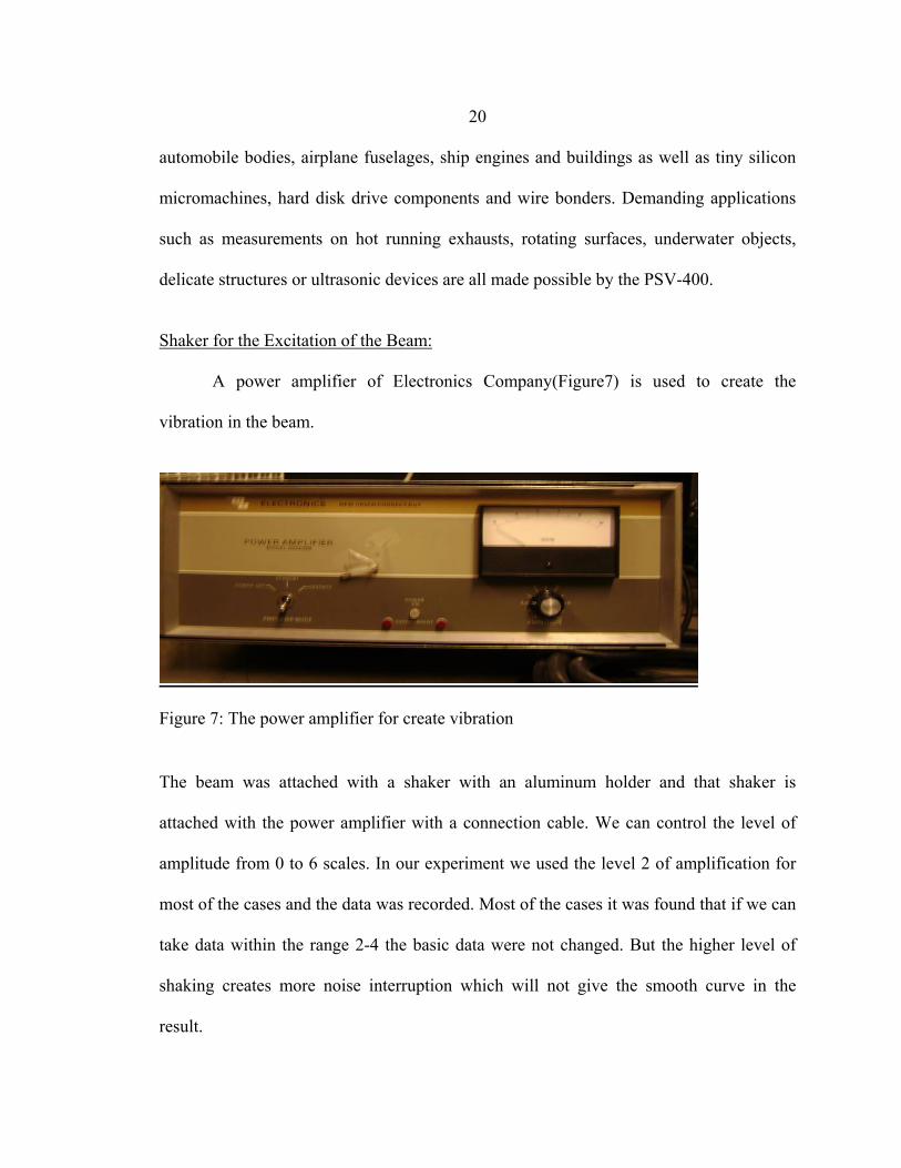
Shaker for the Excitation of the Beam:

A power amplifier of Electronics Company(Figure7) is used to create the

vibration in the beam.

Figure 7: The power amplifier for create vibration The beam was attached with a shaker with an aluminum holder and that shaker is

attached with the power amplifier with a connection cable. We can control the level of

amplitude from 0 to 6 scales. In our experiment we used the level 2 of amplification for

most of the cases and the data was recorded. Most of the cases it was found that if we can

take data within the range 2-4 the basic data were not changed. But the higher level of

shaking creates more noise interruption which will not give the smooth curve in the

result.

21

.

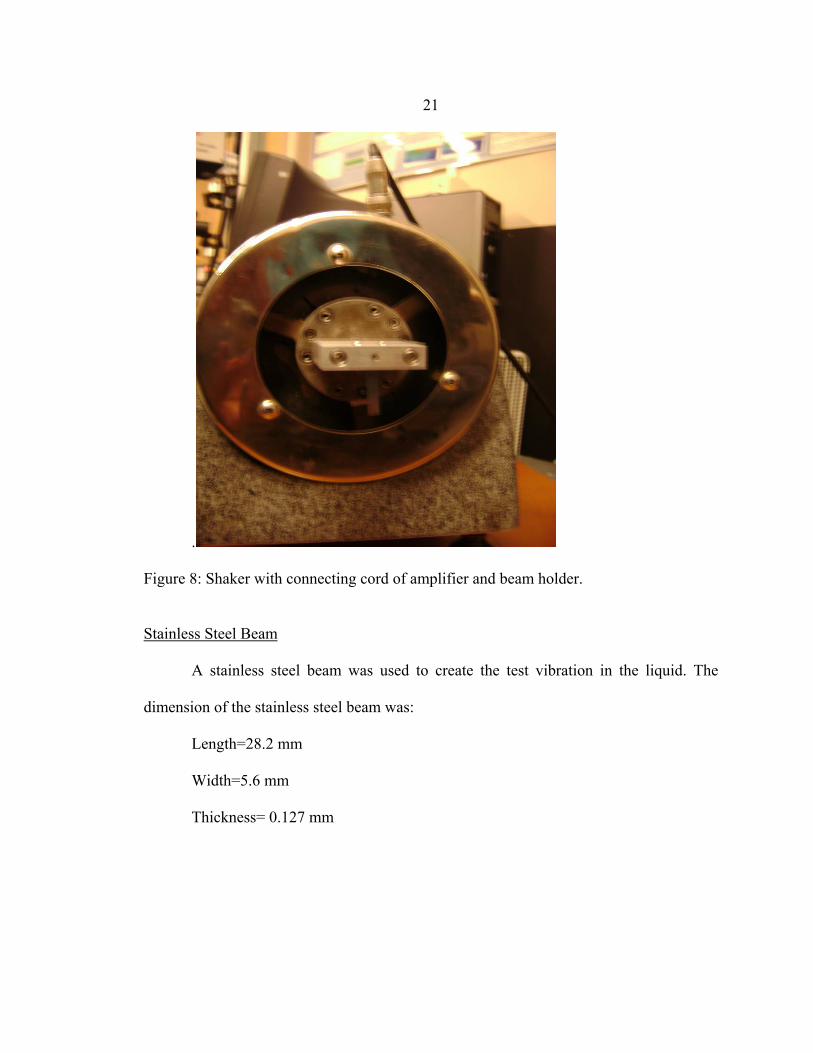
Figure 8: Shaker with connecting cord of amplifier and beam holder. Stainless Steel Beam

A stainless steel beam was used to create the test vibration in the liquid. The

dimension of the stainless steel beam was:

Length=28.2 mm

Width=5.6 mm

Thickness= 0.127 mm

22

Mass of Aluminum

An inverse ‘T’ shaped piece of material was attached with the beam in

configuration A when we placed the beam in horizontal form. The dimensions and the

weight of the aluminum beam are given below:

Figure 9: The T shaped Aluminum mass of configuration A.

Height [lower half] , H1= 7.8 mm

Length [lower half] ,L1 = 15.56 mm Height [upper half],H2 = 7.48 mm

Length [upper half] L2 = 5.26 mm Thickness T2= 3.57 mm

H 1

T2

H 1

T 1

L 1

L1

23

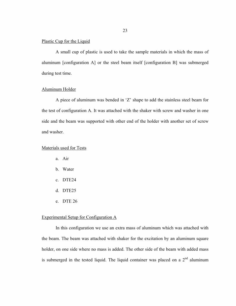
Plastic Cup for the Liquid

A small cup of plastic is used to take the sample materials in which the mass of

aluminum [configuration A] or the steel beam itself [configuration B] was submerged

during test time.

Aluminum Holder

A piece of aluminum was bended in ‘Z’ shape to add the stainless steel beam for

the test of configuration A. It was attached with the shaker with screw and washer in one

side and the beam was supported with other end of the holder with another set of screw

and washer.

Materials used for Tests

a. Air

b. Water

c. DTE24

d. DTE25

e. DTE 26

Experimental Setup for Configuration A

In this configuration we use an extra mass of aluminum which was attached with

the beam. The beam was attached with shaker for the excitation by an aluminum square

holder, on one side where no mass is added. The other side of the beam with added mass

is submerged in the tested liquid. The liquid container was placed on a 2nd aluminum

24

made holder by which we can change the container height to adjust the submerged part of

the mass all time at a constant level.

After adjusting the liquid level the Polytec laser vibrometer which was keeping

started for warm up for half an hour was adjusted with the beam. The scanner head of the

vibrometer was placed vertically so that the beam would be positioned on the middle of

the beam which was in horizontal position. The liquid container would be filling out with

oil or test liquid through the burette.

Experimental Setup for Configuration B

In this configuration we removed the extra mass of aluminum which was attached

with the stainless beam. The beam was attached with shaker for the excitation by an

aluminum square holder, on one side where no mass is added and the shaker would be

positioned in such a horizontal way that the beam itself come in the vertical position. The

other side of the beam without mass is submerged in the tested liquid. The liquid

container was placed on a 2nd aluminum made holder by which we can change the

container height to adjust the submerged part of the mass all time at a constant level.

25

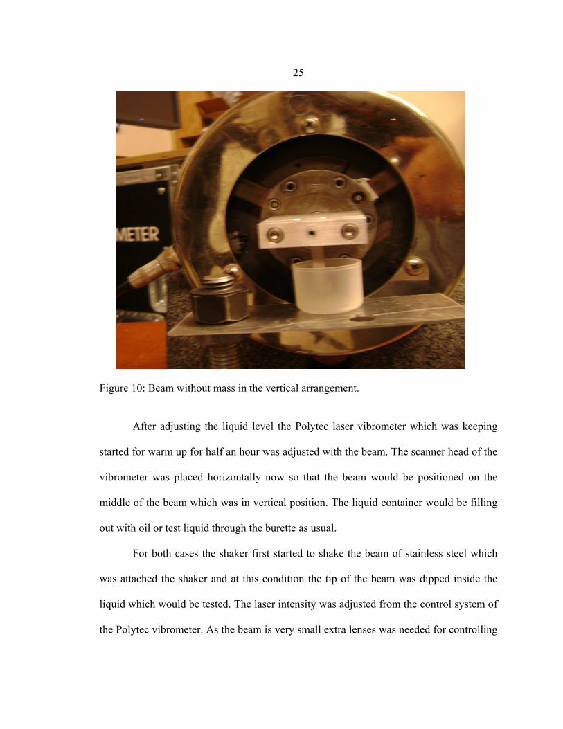
Figure 10: Beam without mass in the vertical arrangement.

After adjusting the liquid level the Polytec laser vibrometer which was keeping

started for warm up for half an hour was adjusted with the beam. The scanner head of the

vibrometer was placed horizontally now so that the beam would be positioned on the

middle of the beam which was in vertical position. The liquid container would be filling

out with oil or test liquid through the burette as usual.

For both cases the shaker first started to shake the beam of stainless steel which

was attached the shaker and at this condition the tip of the beam was dipped inside the

liquid which would be tested. The laser intensity was adjusted from the control system of

the Polytec vibrometer. As the beam is very small extra lenses was needed for controlling

26

the focus of the laser. After the adjustment of the laser beam, the scanning was done in

acquisition mode.

Before complete the scanning, we had to select the area and the scanning

reference points on which we wanted the data to be taken. The data taken in the

acquisition mode was converted to presentation mode so that we can get the frequency

response of the vibrating beam. We here can see the 3D movement or the harmonic

frequency mode. By this graphical picture we can find out the peck of the resonance

frequency as well as the shape of the vibration wave.

27

CHAPTER 4

RESULTS AND DISCUSSION

Configuration A

First, the resonant frequency of the beam in air was calculated using the simple

closed form solution for cantilever beam with concentrate load at the end. The calculated

resonant frequency in the air that measured with the vibrometer was very close and the

difference was within 1%. This result serves as a calibration of the vibrometer system.

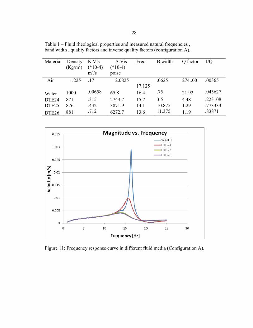
The results obtained for configuration A are given in Table 1 and Figures 11-13.

Table 1 also shows the rheological properties of the fluids. Water has the lowest viscosity

while DTE 26 oil has the highest viscosity among all the fluids. Figure 3a shows the

frequency response curves when the end mass was submerged in all the four fluids as

well as in air. It is evident that the velocity amplitude decreases as the viscosity of the

fluid. It is also observed that the resonant frequency of the beam and the quality factor (½

amplitude bandwidth over the resonant frequency) both decrease with the viscosity of the

fluid. The resonant frequency seems to decrease linearly, while the quality factor (q-

factor) decreases abruptly with increase in viscosity from water to oil.

28

Table 1 – Fluid rheological properties and measured natural frequencies , band width , quality factors and inverse quality factors (configuration A). Material Density

(Kg/m3) K.Vis (*10-4) m2/s

A.Vis (*10-4) poise

Freq B.width Q factor 1/Q

Air 1.225 .17 2.0825 17.125

.0625 274..00 .00365

Water 1000 .00658 65.8 16.4 .75 21.92 .045627 DTE24 871 .315 2743.7 15.7 3.5 4.48 .223108 DTE25 876 .442 3871.9 14.1 10.875 1.29 .773333 DTE26 881 .712 6272.7 13.6 11.375 1.19 .83871

Figure 11: Frequency response curve in different fluid media (Configuration A).

29

Absolute viscosity (x10‐4) Poise

Resonant Freq, Hz

4

6

8

10

12

14

16

18

20

22

24

0 1000 2000 3000 4000 5000 6000 7000

Water DTE24

DTE25 DTE26

Figure 12: Resonant Frequency variation with viscosity (Configuration A).

0.00

5.00

10.00

15.00

20.00

25.00

0 1000 2000 3000 4000 5000 6000 7000

Absolute  viscosity  (x10 ‐4) Poise

Quality Factor

Water

DTE24

DTE25 DTE26

Figure 13: Quality factor (Q) variation with viscosity (Configuration A).

30

All the results of experiment in configuration A is listed in the table 1 and consequently

we plotted all the graphs in figure 11,12 and 13.

The resonance frequencies of the liquids in this configuration are very close to

each other and it varies from 13 to 17 Hz. So this configuration is not much convenient

with respect to the configuration B where frequency range or difference is much higher.

So within these two configurations, B is much more convenient to use.

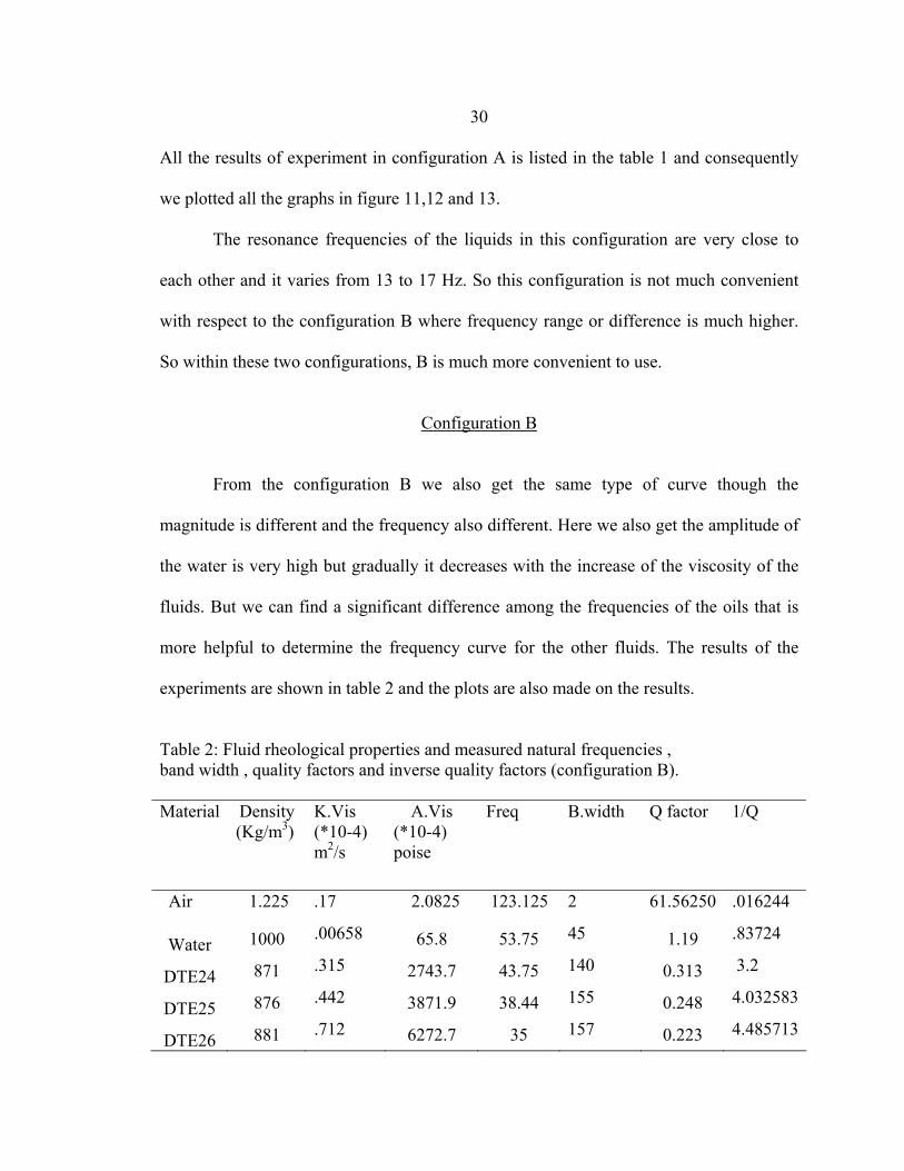
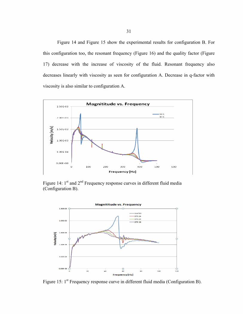
Configuration B

From the configuration B we also get the same type of curve though the

magnitude is different and the frequency also different. Here we also get the amplitude of

the water is very high but gradually it decreases with the increase of the viscosity of the

fluids. But we can find a significant difference among the frequencies of the oils that is

more helpful to determine the frequency curve for the other fluids. The results of the

experiments are shown in table 2 and the plots are also made on the results.

Table 2: Fluid rheological properties and measured natural frequencies , band width , quality factors and inverse quality factors (configuration B). Material Density

(Kg/m3) K.Vis (*10-4) m2/s

A.Vis (*10-4) poise

Freq B.width Q factor 1/Q

Air 1.225 .17 2.0825 123.125 2 61.56250 .016244

Water 1000 .00658 65.8 53.75 45 1.19 .83724

DTE24 871 .315 2743.7 43.75 140 0.313 3.2

DTE25 876 .442 3871.9 38.44 155 0.248 4.032583

DTE26 881 .712 6272.7 35 157 0.223 4.485713

31

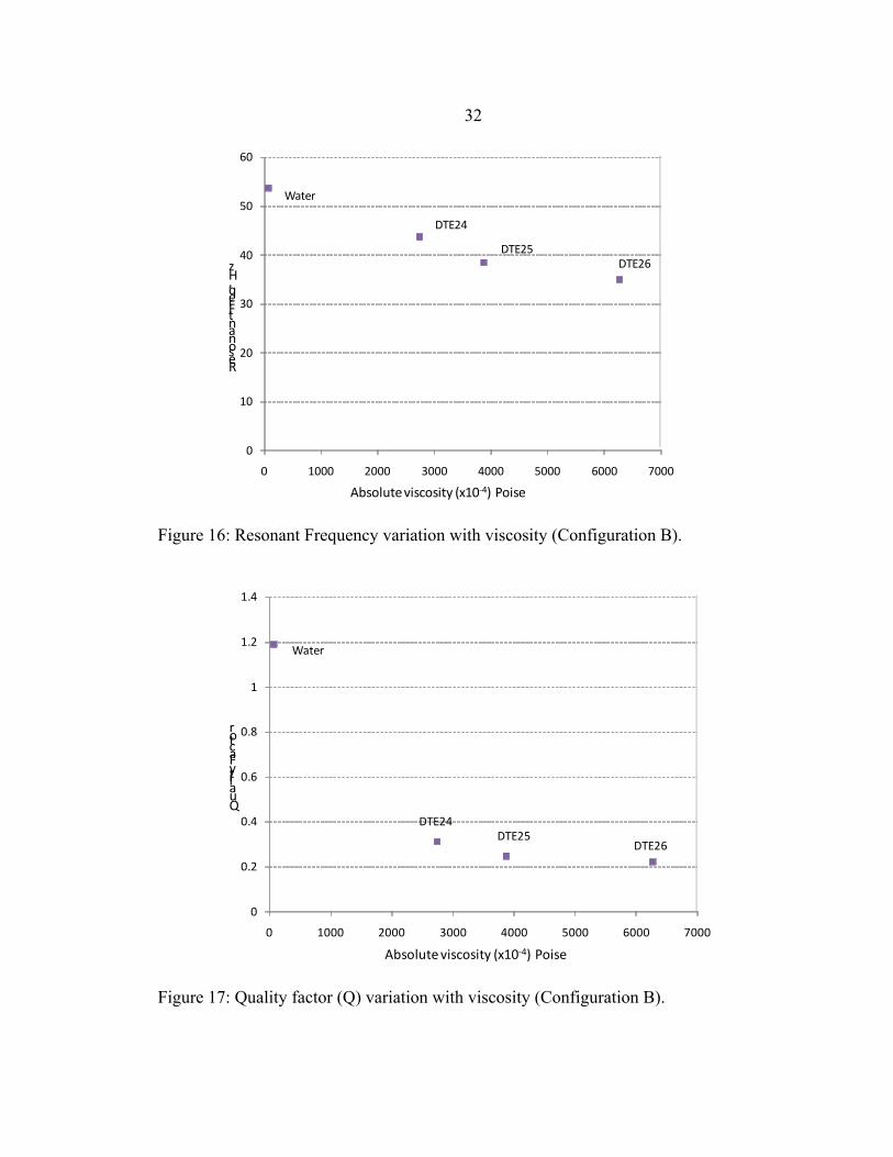
Figure 14 and Figure 15 show the experimental results for configuration B. For

this configuration too, the resonant frequency (Figure 16) and the quality factor (Figure

17) decrease with the increase of viscosity of the fluid. Resonant frequency also

decreases linearly with viscosity as seen for configuration A. Decrease in q-factor with

viscosity is also similar to configuration A.

Figure 14: 1st and 2nd Frequency response curves in different fluid media (Configuration B).

Figure 15: 1st Frequency response curve in different fluid media (Configuration B).

32

0

10

20

30

40

50

60

0 1000 2000 3000 4000 5000 6000 7000

Absolute viscosity (x10‐4) Poise

Resonant Freq, Hz

Water

DTE24

DTE25DTE26

Figure 16: Resonant Frequency variation with viscosity (Configuration B).

0

0.2

0.4

0.6

0.8

1

1.2

1.4

0 1000 2000 3000 4000 5000 6000 7000

Absolute viscosity (x10‐4) Poise

Quality Factor

Water

DTE24DTE25

DTE26

Figure 17: Quality factor (Q) variation with viscosity (Configuration B).

33

Immersions in liquid result in viscous damping of the system that causes change

in q-factor(figure17). In addition, the density of the fluid increases the effective weight of

the beam thereby changing the overall resonant frequency. These experimental

observations will be used to find closed form theoretical equations relating resonant

frequency, q-factor, density, and viscosity so that these equations can be used along with

measurement using any unknown fluid to find its rheological properties.

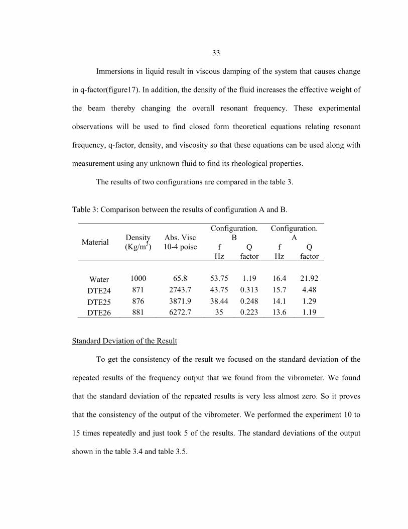
The results of two configurations are compared in the table 3. Table 3: Comparison between the results of configuration A and B.

Configuration.

B Configuration.

A Material Density (Kg/m3)

Abs. Visc 10-4 poise f

Hz Q

factor f

Hz Q

factor

Water 1000 65.8 53.75 1.19 16.4 21.92 DTE24 871 2743.7 43.75 0.313 15.7 4.48 DTE25 876 3871.9 38.44 0.248 14.1 1.29 DTE26 881 6272.7 35 0.223 13.6 1.19

Standard Deviation of the Result

To get the consistency of the result we focused on the standard deviation of the

repeated results of the frequency output that we found from the vibrometer. We found

that the standard deviation of the repeated results is very less almost zero. So it proves

that the consistency of the output of the vibrometer. We performed the experiment 10 to

15 times repeatedly and just took 5 of the results. The standard deviations of the output

shown in the table 3.4 and table 3.5.

34

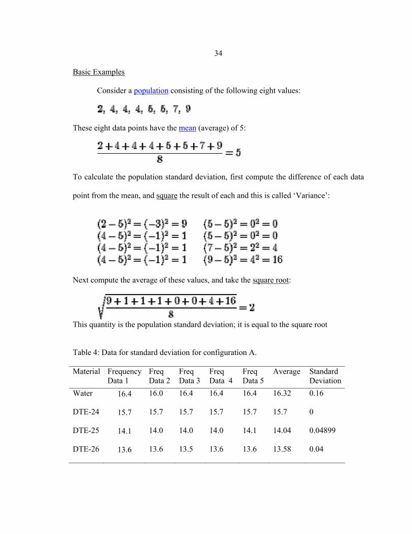
Basic Examples

Consider a population consisting of the following eight values:

These eight data points have the mean (average) of 5:

To calculate the population standard deviation, first compute the difference of each data

point from the mean, and square the result of each and this is called ‘Variance’:

Next compute the average of these values, and take the square root:

This quantity is the population standard deviation; it is equal to the square root Table 4: Data for standard deviation for configuration A.

Material Frequency Data 1

Freq Data 2

Freq Data 3

Freq Data 4

Freq Data 5

Average Standard Deviation

Water 16.4 16.0 16.4 16.4 16.4 16.32 0.16

DTE-24 15.7 15.7 15.7 15.7 15.7 15.7 0

DTE-25 14.1 14.0 14.0 14.0 14.1 14.04 0.04899

DTE-26 13.6 13.6 13.5 13.6 13.6 13.58 0.04

35

Table 5: Data for standard deviation for configuration B.

Material Frequency Data 1

Freq Data 2

Freq Data 3

Freq Data 4

Freq Data 5

Average Standard Deviation

Water 53.75 53.75 53.75 53.75 53.75 53.75 0

DTE-24 43.75 43.70 43.75 43.73 43.75 43.736 .019596

DTE-25 38.44 38.44 38.44 38.44 38.44 38.44 0

DTE-26 35 35 35 35.1 35.1 35.04 0.04899

Mathematical Solution of the Frequency in Air (Configuration A)

L=28.2mm,

B=5.6mm, T=0.127mm

a=24.76mm

b= 3.44mm

m=1.7098 gm [with mass]

P=mg

E=200 GPa

I=BT3/12 [moment of inertia]

δ = Pa2(3L-a)/6EI [beam deflection]

wn=sqrt(g/δ) [ natural frequency] f=wn/2π= 17.82 Hz [experimental f= 17.125 Hz]

36

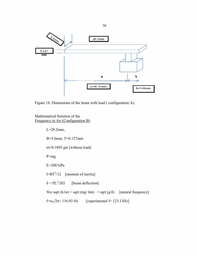
Figure 18: Dimensions of the beam with load ( configuration A).

Mathematical Solution of the Frequency in Air (Configuration B)

L=28.2mm,

B=5.6mm, T=0.127mm

m=0.1895 gm [without load]

P=mg

E=200 GPa

I=BT3/12 [moment of inertia]

δ = PL3/3EI [beam deflection]

Wn=sqrt (k/m) = sqrt (mg/ δm) = sqrt (g/δ) [natural frequency] f=wn/2π= 116.93 Hz [experimental f= 123.13Hz]

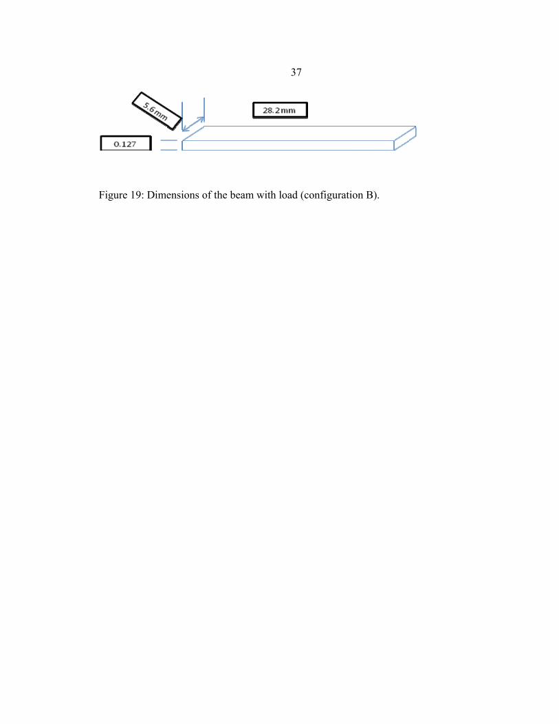
37

Figure 19: Dimensions of the beam with load (configuration B).

38

CHAPTER 5

FINITE ELEMENT ANALYSIS

The finite element method involves modeling the structure using small

interconnected elements. A displacement function is associated with each finite element.

Every interconnected element is linked, directly or indirectly, to every other element

through common or shared interfaces, including nodes and/ or boundary lines and or

surfaces. By using known stress/strain properties for the material making up the structure,

one can determine the behavior of a given node in terms of the properties of every other

element in the structure. The total set of equations describing the behavior of each node

results a series of algebraic equations best expressed in matrix notation.

There are two general direct approaches traditionally associated with the finite

element method as applied to structural mechanics problems. One approach, called the

force or flexibility method, which method uses internal forces as the unknowns of the

problem. To obtain the governing equations, first the equilibrium equations are used.

Then necessary additional equations are found by introducing compatibility equations.

The result is a set of equations for determining the redundant or unknown forces.

The second approach, called the displacement, or stiffness method, which

assumes the displacements of the nodes as the unknowns of the problem. For instance,

compatibility conditions requiring that elements connected at a common node, along a

common edge, or on a common surface before loading remain connected at that node,

edge, or surface after deformation takes place are initially satisfied. Then the governing

39

equations are expressed in terms of nodal displacements using the equations of

equilibrium and an applicable law relating forces to displacements.

These two direct approaches in different unknowns (forces and displaces) in the

analysis and different matrices associated with their formulations (flexibilities or

stiffness). It has been shown that, for computational purposes, the displacement (or

stiffness) method is more desirable. Furthermore a vast majority of general purpose finite

element programs have incorporated the displacement formulation for solving structural

problems. Consequently, only the displacement method will be used throughout this

experiment.

After testing by vibrometer we try the finite element analysis to predict the

dynamic response of a cantilever beam as shown in Figure 20. The beam is partially

submerged under various viscous media, e.g., water, and other three types of DTE

lubricating oil. The numerical prediction was then compared with experimental results

already performed. Numerical analysis was also conducted to investigate the variation in

modal response with changing the fluid properties and other parameters. The ultimate

goal of this project is to design the optimized microcantilever to measure the rheological

properties of viscous fluid.

40

Viscous media

Polytec Vibrometer

Stainless steel beam

Base vibrations at 

sweeping frequencies.

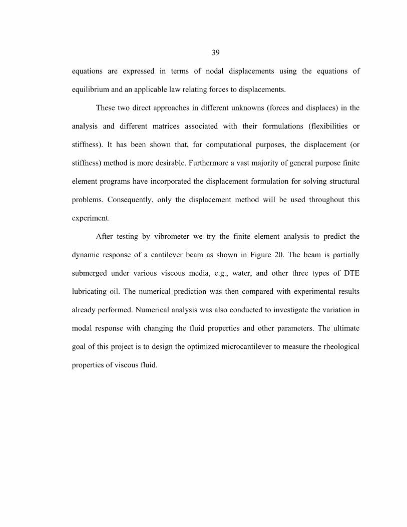
 Figure 20: Experimental setup to predict modal response of cantilever beam. Procedure

The commercially available FEA package ANSYS was used to develop the finite

element model of a beam partially submerged under fluid. The beam was considered to

be a two dimensional plain-strain problem. Therefore, only the longitudinal cross-section

of the beam was modeled as shown in Figure 25 below. The beam and fluid were

simulated using 2D structural solid (Plane 42) and contained fluid (Fluid 79) elements,

respectively. The fluid element (Fluid 79) was particularly well suited for solid-fluid

interaction. For academic interest, fluid region was also simulated using 2D axisymmetric

harmonic acoustic fluid element (Fluid 29). This element is also suitable for modeling the

fluid medium and the interface in fluid/structure interaction problems. However, the

element has no option to include viscous effect directly. Whereas the viscous effect could

be indirectly included using the bulk modulus and density. These are described below.

41

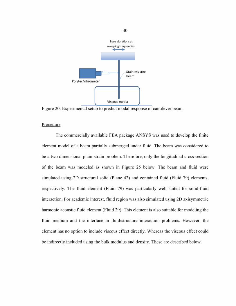
Plane 42 Element Description. PLANE 42 is used for 2-D modeling of solid structures. The

element can be used either as a plane element (plane stress or plane strain) or as an

axisymmetric element. The element is defined by four nodes having two degrees of

freedom at each node: translations in the nodal x and y directions. The element has

plasticity, creep, swelling, stress stiffening, large deflection, and large strain capabilities.

An option is available to suppress the extra displacement shapes.

Figure 21: PLANE42 Geometry.

Input Data. The geometry, node locations, and the coordinate system for this

element are shown in figure21. The element input data includes four nodes, a thickness

(for the plane stress option only) and the orthotropic material properties. Orthotropic

material directions correspond to the element coordinate directions. The element

coordinate system orientation is as described in Coordinate Systems.

Element loads are described in Node and Element Loads. Pressures may be input

as surface loads on the element faces as shown by the circled numbers on Figure 4.a.

Positive pressures act into the element. Temperatures and fluences may be input as

42

element body loads at the nodes. The node I temperature T(I) defaults to TUNIF. If all

other temperatures are unspecified, they default to T(I). For any other input pattern,

unspecified temperatures default to TUNIF. Similar defaults occurs for fluence except

that zero is used instead of TUNIF.

The nodal forces, if any, should be input per unit of depth for a plane analysis

(suppress the extra displacement shapes. KEYOPT(5) and KEYOPT(6) provide except

for KEYOPT(3) = 3) and on a full 360° basis for an axisymmetric analysis. KEYOPT(2)

is used to include or various element printout options. Initial state conditions previously

handled via the ISTRESS command will be discontinued for this element. The

INISTATE command will provide increased functionality, but only via the Current

Technology elements (180,181, etc. ). To continue using Initial State conditions in future

versions of ANSYS, we considered switching to the appropriate Current Technology

element. We can include the effects of pressure load stiffness in a geometric nonlinear

analysis using SOLCONTROL, INCP. Pressure load stiffness effects are included in

linear eigenvalue buckling automatically. If an unsymmetric matrix is needed for pressure

load stiffness effects, we have to use NROPT, UNSYM.

Output Data. The solution output associated with the element is in two forms:

• Nodal displacements included in the overall nodal solution

• Additional element output also available “PLANE.

The element stress directions are parallel to the element coordinate system. Surface

stresses are available on any face. Surface stresses on face IJ, for example, are defined

parallel and perpendicular to the IJ line and along the Z axis for a plane analysis or in the

43

hoop direction for an axisymmetric analysis. A general description of solution output is

given in Solution Output.

Figure 22: PLANE 42 stress output. For axisymmetric solutions with KEYOPT(1) = 0, the X, Y, Z, and XY stress and strain

outputs correspond to the radial, axial, hoop, and in-plane shear stresses and strains,

respectively. As shown in Figure22, "PLANE42 Geometry" and the Y-axis must be the

axis of symmetry for axisymmetric analyses. An axisymmetric structure should be

modeled PLANE42 Assumptions and Restrictions:

• The area of the element must be nonzero.

• The element must lie in a global X-Y plane in the +X quadrants.

• A triangular element may be formed by defining duplicate K and L node

numbers (see Triangle, Prism and Tetrahedral Elements).

• The extra shapes are automatically deleted for triangular elements so that a

constant strain element results.

• Surface stress printout is valid only if the conditions described in Element

Solution are met.

The only special feature allowed is stress stiffening.

44

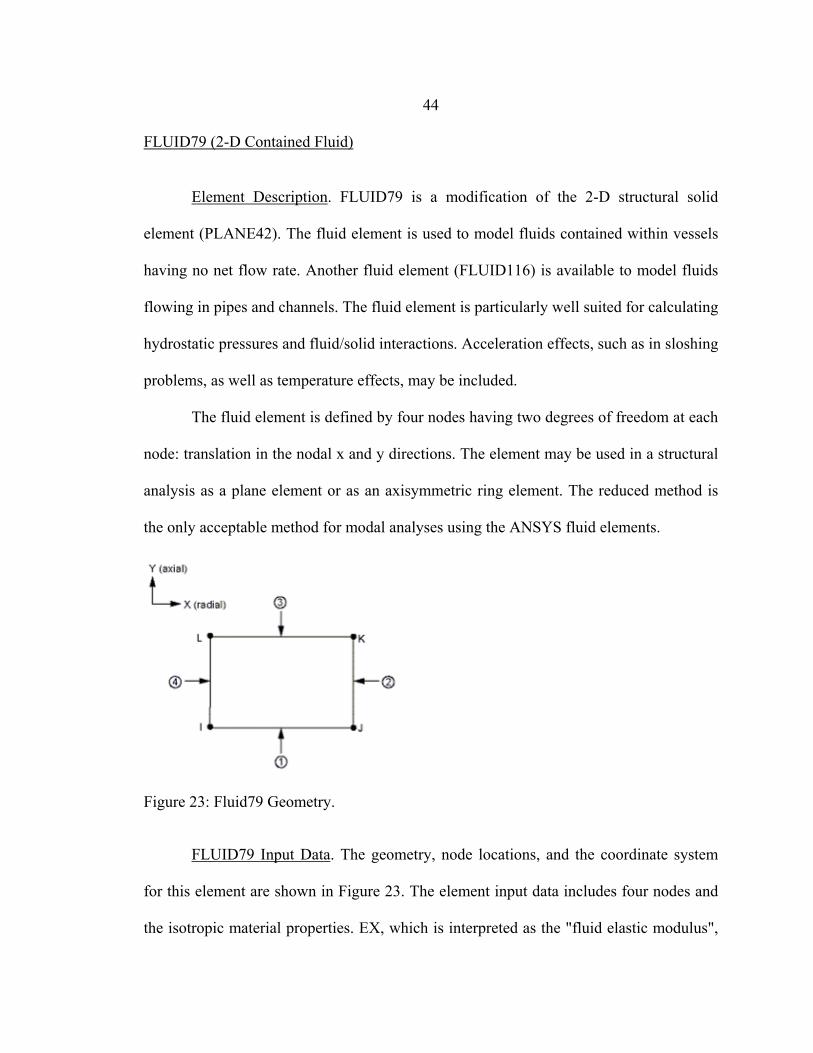
FLUID79 (2-D Contained Fluid)

Element Description. FLUID79 is a modification of the 2-D structural solid

element (PLANE42). The fluid element is used to model fluids contained within vessels

having no net flow rate. Another fluid element (FLUID116) is available to model fluids

flowing in pipes and channels. The fluid element is particularly well suited for calculating

hydrostatic pressures and fluid/solid interactions. Acceleration effects, such as in sloshing

problems, as well as temperature effects, may be included.

The fluid element is defined by four nodes having two degrees of freedom at each

node: translation in the nodal x and y directions. The element may be used in a structural

analysis as a plane element or as an axisymmetric ring element. The reduced method is

the only acceptable method for modal analyses using the ANSYS fluid elements.

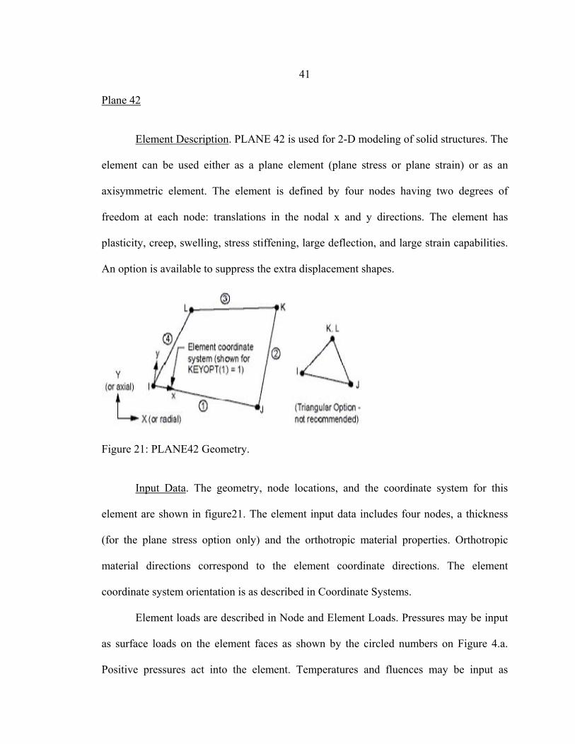
Figure 23: Fluid79 Geometry.

FLUID79 Input Data. The geometry, node locations, and the coordinate system

for this element are shown in Figure 23. The element input data includes four nodes and

the isotropic material properties. EX, which is interpreted as the "fluid elastic modulus",

45

should be the bulk modulus of the fluid (approximately 300,000 psi for water). The

viscosity property (VISC) is used to compute a damping matrix for dynamic analyses

(typical viscosity value for water is 1.639 x 10-7 lb-sec/in2). Element loads are described

in Node and Element Loads. Pressures may be input as surface loads on the element faces

as shown by the circled numbers on Figure23. Positive pressures act into the element.

Temperatures may be input as element body loads at the nodes. The node I temperature

T(I) defaults to TUNIF. If all other temperatures are unspecified, they default to T(I). For

any other input pattern, unspecified temperatures default to TUNIF.

FLUID79 Output Data. The solution output associated with the element is in two

forms:

• Degree of freedom results included in the overall nodal solution [19]

• Additional element output available in FLUID79 Element Output Definitions.

The pressure and temperature are evaluated at the element centroid. Nodal forces and

reaction forces are on a full 360° basis for axisymmetric models. A general description of

solution output is given in Solution Output.

FLUID79 Assumptions and Restrictions:

• The area of the element must be positive.

• The fluid element must lie in an X-Y plane as shown in and the Y-axis must

be the axis of symmetry for axisymmetric analyses.

• An axisymmetric structure should be modeled in the +X quadrants.

• Radial motion should be constrained at the centerline.

46

• Usually the Y-axis is oriented in the vertical direction with the top surface at

Y = 0.0.

• The element temperature is taken to be the average of the nodal temperatures.

• Elements should be rectangular whenever possible, as results are known to be

of lower quality for some cases using nonrectangular shapes.

• Axisymmetric elements should always be rectangular.

• The nonlinear transient dynamic analysis should be used instead of the linear

transient dynamic analysis for this element.

• A very small stiffness (EX x 1.0E-9) is associated with the shear and rotational strains to ensure static stability. Only the lumped mass matrix is available.

FLUID 29

Element Description. FLUID 29 is used for modeling the fluid medium and the

interface in fluid/structure interaction problems. Typical applications include sound wave

propagation and submerged structure dynamics. The governing equation for acoustics,

namely the 2-D wave equation, has been discretized taking into account the coupling of

acoustic pressure and structural motion at the interface. The element has four corner

nodes with three degrees of freedom per node: translations in the nodal x and y directions

and pressure. The translations, however, are applicable only at nodes that are on the

interface. Acceleration effects, such as in sloshing problems, may be included.

47

Figure 24: FLUID29 Geometry. The element has the capability to include damping of sound absorbing material at the

interface. The element can be used with other 2-D structural elements to perform

unsymmetric or damped modal, full harmonic response and full transient method. When

there is no structural motion, the element is also applicable to static, modal and reduced

harmonic response analyses.

FLUID29 Input Data. The geometry, node locations, and the coordinate system

for this element are shown in Figure24. The element is defined by four nodes, the number

of harmonic waves (MODE on the MODE command), the symmetry condition (ISYM on

the MODE command), a reference pressure, and the isotropic material properties.. The

reference pressure (PREF) is used to calculate the element sound pressure level (defaults

to 20x10-6 N/m2). The speed of sound in the fluid is input by SONC where k is the bulk

modulus of the fluid (Force/Area) and ρo is the mean fluid density (Mass/Volume) (input

as DENS). The dissipative effect due to fluid viscosity is neglected, but absorption of

sound at the interface is accounted for by generating a damping matrix using the surface

area and boundary admittance at the interface. Experimentally measured values of the

48

boundary admittance for the sound absorbing material may be input as material property

MU. We recommend MU values from 0.0 to 1.0; however, values greater than 1.0 are

allowed. MU = 0.0 represents no sound absorption and MU = 1.0 represents full sound

absorption. DENS, SONC and MU are evaluated at the average of the nodal

temperatures.

Nodal flow rates, if any, may be specified using the F command where both the

real and imaginary components may be applied. Nodal flow rates should be input per unit

of depth for a plane analysis and on a 360° basis for an axisymmetric analysis.

Element loads are described in Node and Element Loads. Fluid-structure

interfaces (FSI) may be flagged by surface loads at the element faces as shown by the

circled numbers on Figure 24. Specifying the FSI label (without a value) [SF, SFA, SFE]

will couple the structural motion and fluid pressure at the interface. Deleting the FSI

specification [SFDELE, SFADELE, SFEDELE] removes the flag. The flag specification

should be on the fluid elements at the interface. The surface load label IMPD with a value

of unity should be used to include damping that may be present at a structural boundary

with a sound absorption lining. A zero value of IMPD removes the damping calculation.

The displacement degrees of freedom (UX and UY) at the element nodes not on the

interface should be set to zero to avoid zero-pivot warning messages.

Temperatures may be input as element body loads at the nodes. The node I

temperature T(I) defaults to TUNIF. If all other temperatures are unspecified, they default

to T(I). For any other input pattern, unspecified temperatures default to TUNIF.

49

KEYOPT (2) is used to specify the absence of a structure at the interface and, therefore,

the absence of coupling between the fluid and structure. Since the absence of coupling

produces symmetric element matrices, a symmetric eigensolver [MODOPT] may be used

within the modal analysis. However, for the coupled (unsymmetric) problem, a

corresponding unsymmetric eigensolver [MODOPT] must be used.

Vertical acceleration (ACELY on the ACEL command) is needed for the gravity

regardless of the value of MODE, even for a modal analysis.

FLUID29 Output Data. The solution output associated with the element is in two

forms: Nodal displacements and pressures included in the overall nodal solution.

• Additional element output available in FLUID29 element output definitions.

FLUID29 Assumptions and Restrictions:

• The area of the element must be positive.

• The element must lie in a global X-Y plane as shown in Figure 23.

• All elements must have 4 nodes. A triangular element may be formed by

defining duplicate K and L nodes (see Triangle, Prism and Tetrahedral

Elements).

• The acoustic pressure in the fluid medium is determined by the wave equation

with the following assumptions:

• The fluid is compressible (density changes due to pressure variations).

• Inviscid fluid (no dissipative effect due to viscosity).

• There is no mean flow of the fluid.

50

• The mean density and pressure are uniform throughout the fluid. Note

that the acoustic pressure is the excess pressure from the mean pressure.

• Analyses are limited to relatively small acoustic pressures so that the

changes in density are small compared with the mean density.

The lumped mass matrix formulation [LUMPM,ON] is not allowed for this element.

The beam and fluid elements at the interface shared the same node. The fluid

elements had finer meshing towards the beam to capture the details of fluid motion

during beam vibrations. The applied boundary conditions were as follows (fig25), the

beam was fixed at one end. The fluid nodes at the left and right sides were constrained in

global x-displacement (ux = 0). Similarly, the fluid nodes at the bottom side were also

constrained in global y-displacement (uy =0).

Figure 25: FE model of cantilever beam partially submerged under fluid.

51

The material properties for the beam were considered to be linear elastic.

Therefore, standard modulus of elasticity (E = 200 GPa), density (ρ = 7850 kg/m3) and

Poisson’s ratio (ν = 0.3) were used for stainless steel. The required material properties for

the fluid elements were bulk modulus (B), density (ρf) and viscosity (μ). The actual fluid

properties used in the FE analysis depend on the type of fluid to be simulated. For water,

B = 2.15 GPa, ρf = 1000 kg/m3, and μ = 65.8 x 10-4 poise were used.

Different eigensolvers are available in ANSYS associated with modal analysis.

The “Damp” eigensolver is used to include the viscous effect of the fluid, which

calculates the system damping matrix needed to be included in the fundamental modal

equation as given by:

[ ]{ } [ ]{ } [ ]{ }iiiii MCK φλφλφ2

⎟⎠⎞

⎜⎝⎛−=+

−−

(Eq. 1)

where, [K] = structural stiffness matrix

{φi} = eigenvector

−

iλ = complex eigenvalues = ii jωσ ±

σi = real part of eigenvalues

ωi = imaginary part of eigenvalues (damped circular frequency)

1−=j

[M] = structural mass matrix

The eigensolutions obtained with damp eigensolver, which includes the damping

matrix, are complex number. The ith eigenvalue is stable when σi is negative and unstable

52

when σi is positive. The numerical simulation was performed with specifying the number

of eigensolutions to extract. It also includes the frequency range representing the lower

and upper ends of the frequencies of interest. The numerical output with damp

eigensolver generally includes all possible modes of vibrations, either local or global, of

the solid (beam) and fluid entities. Therefore, the global modes of vibration (or the

resonant frequency) of the beam are determined by visually observing the mode shape,

which has the dominant participation in the transverse direction. Figure26 represents the

mode shapes for 1st resonant frequency.

Figure 26: Mode shape for the 1st resonant vibration in transverse direction.

Results of Analysis

The modal response of the partially submerged beam was numerically predicted

with different fluid properties as requires. For water, the 1st resonant frequency with

53

dominant participation in the transverse direction was found to be 51.5 Hz. And from the

Vibrometer we got this value 53.75Hz. The difference between the numerical and

experimental results is around 4.5%. Additional effort is done provided to numerically

predict the modal response of beam with simulating other DTE viscous fluid. The results

are shown in the table 6 and table 7.

Table 6: Experimental modal response of cantilever beam.

Expt. Results

Density (Kg/m3)

Abs. Visc. (10-4 poise) f

(Hz) Inv. Q factor

Water 1000 65.8 53.75 1.19 DTE24 871 2743.7 43.75 0.313 DTE25 876 3871.9 38.44 0.248 DTE26 881 6272.7 35 0.223

Table 7: Effect of changing Viscosity without changing Bulk Modules.

ANSYS

Density Bulk Modulus Viscosity Real Part Ima. Part Frequency Expt. Freq. Difference

(kg/m3) (Pa) (10-4 Poise) (Hz) (Hz) (Hz) (Hz) (%)

65.80 6.35 50.12 50.52 53.75 6.01

2743.70 3.13 50.47 50.57 43.75 -15.58

3871.90 3.00 49.46 49.55 38.44 -28.90

1000 2.15E+09

6272.00 3.16 48.74 48.84 35.00 -39.55

In the Next parametric calculation we fixed the bulk modules and density of fluid

constant and put the viscosity of the fluids like water,DTE24, DTE25 and DTE 26 to see

how the frequency decrease with only change of viscosity. We found that bulk modules

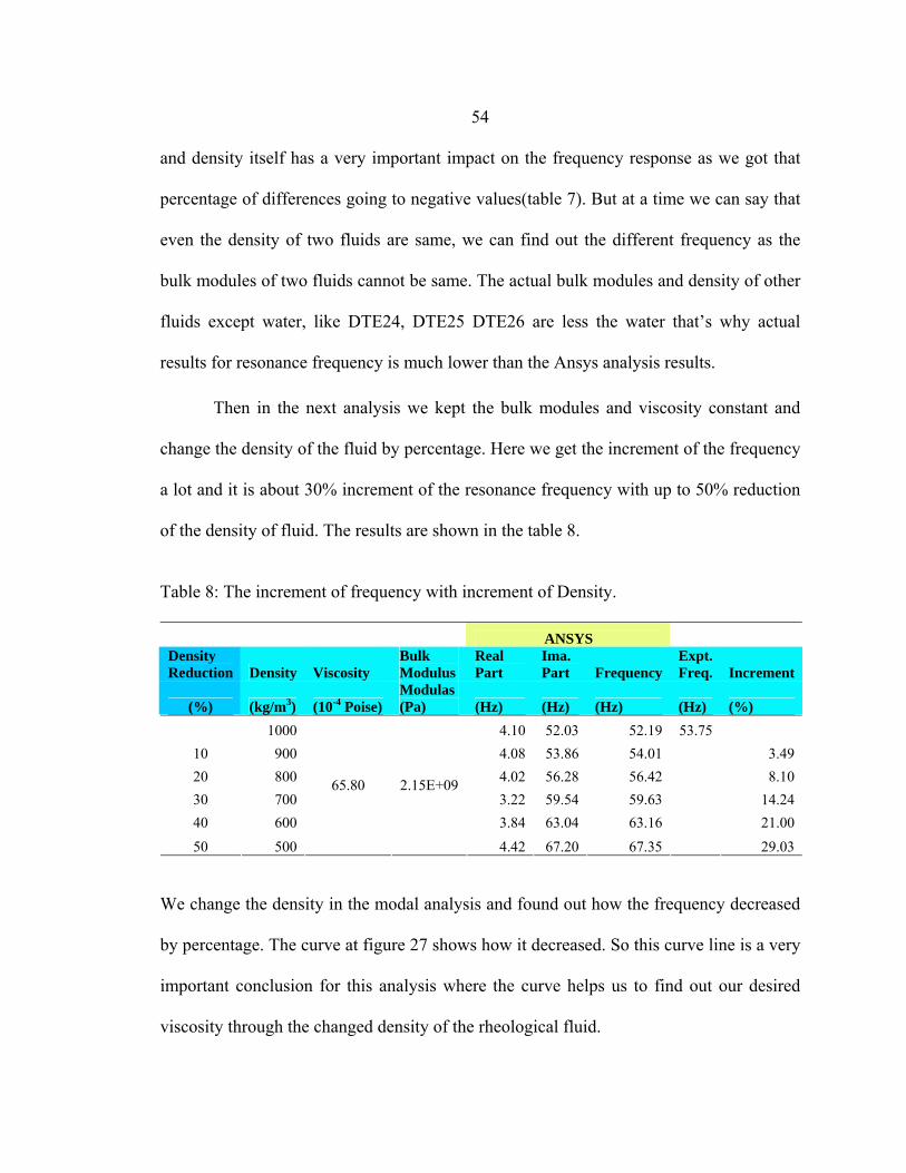
54

and density itself has a very important impact on the frequency response as we got that

percentage of differences going to negative values(table 7). But at a time we can say that

even the density of two fluids are same, we can find out the different frequency as the

bulk modules of two fluids cannot be same. The actual bulk modules and density of other

fluids except water, like DTE24, DTE25 DTE26 are less the water that’s why actual

results for resonance frequency is much lower than the Ansys analysis results.

Then in the next analysis we kept the bulk modules and viscosity constant and

change the density of the fluid by percentage. Here we get the increment of the frequency

a lot and it is about 30% increment of the resonance frequency with up to 50% reduction

of the density of fluid. The results are shown in the table 8.

Table 8: The increment of frequency with increment of Density.

ANSYS Density Reduction Density Viscosity

Bulk Modulus

Real Part

Ima. Part Frequency

Expt. Freq. Increment

(%) (kg/m3) (10-4 Poise) Modulas (Pa) (Hz) (Hz) (Hz) (Hz) (%)

1000 4.10 52.03 52.19 53.75 10 900 4.08 53.86 54.01 3.49 20 800 4.02 56.28 56.42 8.10 30 700 3.22 59.54 59.63 14.24 40 600 3.84 63.04 63.16 21.00 50 500

65.80 2.15E+09

4.42 67.20 67.35 29.03 We change the density in the modal analysis and found out how the frequency decreased

by percentage. The curve at figure 27 shows how it decreased. So this curve line is a very

important conclusion for this analysis where the curve helps us to find out our desired

viscosity through the changed density of the rheological fluid.

55

Figure 27: Increase of frequency by the decrease of density of viscous fluids. Harmonic Solution

To support the results found in Modal analysis we then perform the harmonic

analysis (figure 28) and we again get the resonance frequency of water at 52-53 Hz. So

the result in modal analysis and the result of harmonic analysis (table 9) are similar.

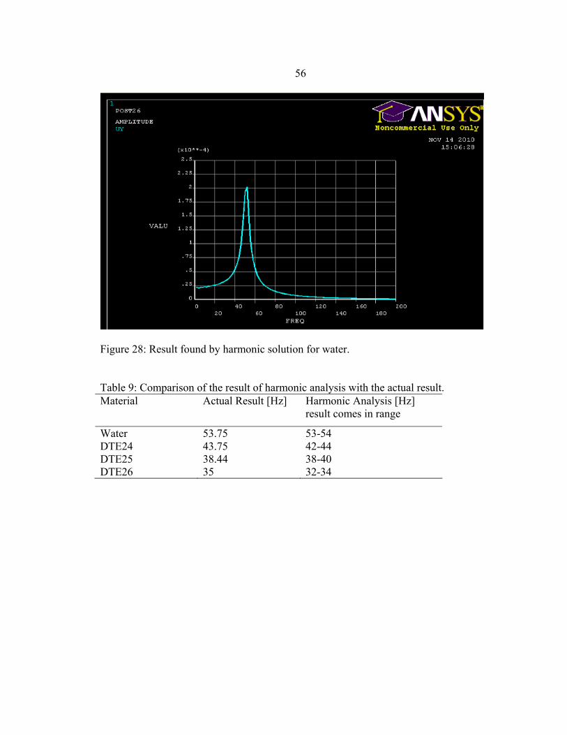
56

Figure 28: Result found by harmonic solution for water. Table 9: Comparison of the result of harmonic analysis with the actual result. Material Actual Result [Hz] Harmonic Analysis [Hz]

result comes in range

Water 53.75 53-54 DTE24 43.75 42-44 DTE25 38.44 38-40 DTE26 35 32-34

57

CHAPTER 6

MEMS DESIGN AND STEPS OF FABRICATION

Our next work is focused on the MEMS fabrication of the micro beam to get the

final device to measure the rheological property of fluids. MEMS represent one of the

today’s most exciting areas of microelectronics activity. MEMS technology has brought

together innovations from many areas of microelectronics only to develop rapidly into a

discipline of its own. Today’s micromachined systems combine the signal processing and

computational capability of analog and digital integrated circuits with a wide variety of

nonelectrical elements, including pressure, temperature and chemical sensors, mechanical

gears and actuators, 3D mirror structures etc. and they have only began to scratch the

surface of biomedical applications.

Now a day there is a continuous push towards automation, miniaturization and

integration throughout the industry and research. With the present acceleration of

technology, microelectromechanical system [MEMS] has become a popular and preferred

means for advances in biotechnology. Within the past couple of years there has been a

drive for micrometer scale. The benefits of the micro-rheology are numerous allowing for

the fast and efficient generation of various statistical data sets on small cell samples in a

short amount of time. The system can be automated and the process can be incorporated

into a larger system for in-line analysis. Therefore the goal of the micro-rheometer is to

establish and exploit the benefits of the micro-world in the development of an automated,

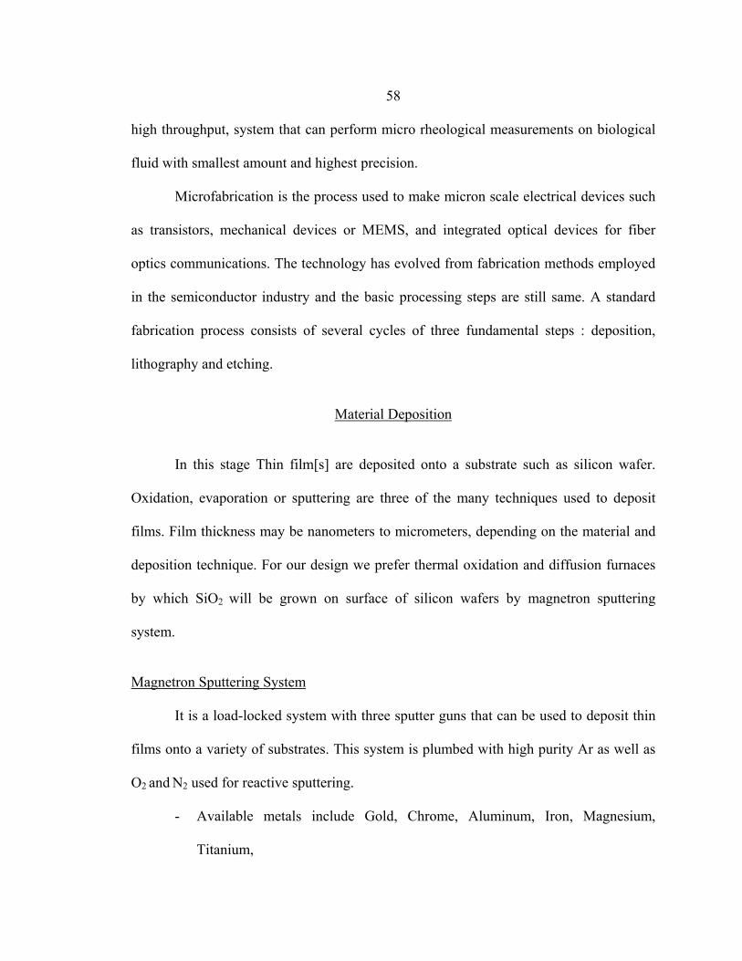
58

high throughput, system that can perform micro rheological measurements on biological

fluid with smallest amount and highest precision.

Microfabrication is the process used to make micron scale electrical devices such

as transistors, mechanical devices or MEMS, and integrated optical devices for fiber

optics communications. The technology has evolved from fabrication methods employed

in the semiconductor industry and the basic processing steps are still same. A standard

fabrication process consists of several cycles of three fundamental steps : deposition,

lithography and etching.

Material Deposition

In this stage Thin film[s] are deposited onto a substrate such as silicon wafer.

Oxidation, evaporation or sputtering are three of the many techniques used to deposit

films. Film thickness may be nanometers to micrometers, depending on the material and

deposition technique. For our design we prefer thermal oxidation and diffusion furnaces

by which SiO2 will be grown on surface of silicon wafers by magnetron sputtering

system.

Magnetron Sputtering System

It is a load-locked system with three sputter guns that can be used to deposit thin

films onto a variety of substrates. This system is plumbed with high purity Ar as well as

O2 and N2 used for reactive sputtering.

- Available metals include Gold, Chrome, Aluminum, Iron, Magnesium,

Titanium,

59

- Dielectrics include SiO2, CrN, AlN, MgO, MgF2…

Manual Spin Coater

It can be used to coat a variety of liquid based materials onto flat substrates.

Materials such as photo resist, SU8, SOG [spin-on glass], Teflon, PTFE, PMMA, PMDS

etc. can be deposited in this fashion.

Photolithography

Lithography is the process of patterning a photosensitive material using a mask.

The mask is akin to a negative in photography. A photosensitive material (photoresist) on

the substrate is illuminated through the mask to transfer the mask pattern to the

underlying material.

Contact Aligner. It is used for patterning 1.0 µm features onto substrates. Uses a

collimated broadband mercury light source for exposure. Includes features for backside

alignment.

Programmable Spin Coater. A computer controlled spin coater that is used to coat

substrates with photoresist. The resist thickness is controlled by the spin speed and spin

duration. At present we can coat with 1-2 µm thick photoresist layer using Shipley 1813

resist. Thicker resist can be obtained.

60

Material Etching

Material etching means the selective removal of unwanted portions of a patterned

layer.

Plasma Etcher. March CS 1700 plasma etcher is available in our lab. It can etch

silicon oxide and nitride as well as organic films using CF4 , SF6 , and / or O2. It can also

be used with Ar for de-scum etching.

Wet Benches. There are 2 types of wet benches.

1. Lithography wetbench: It is used for photoresist development, general solvent

work , Also contains the headway manual coater.

2. Acid/ Base wetbench: it is the general purpose bench used for wafer cleaning

and chemical etching.

Characterization

1. Nanospectrometer:

- Measures SiO2, Si3N4 and photoresist films on silicon substrates.

2. Ambios Stylus surface profilometer:

- A manual stylus profilometer used to measure thin film step heights. It can

measure 10’s of nanometers to microns in heights.

3. Inspection Microscopes

- A Nikon reflection microscope with a Camera /CCD port. Objectives

10X-100X magnification.

- An Olympus reflection / transmission microscope is also available.

61

Packaging

1. Wafer Saw:

- It is a programmable Micro Automation saw used to dice thin substrates.

2. Wire Bonders:

- Wedge bonder with heated stage. Configured with 1.0 mil gold or

aluminum wire for electronic bonding.

Fabrication Sequences

1. Blank 4 in DSP wafer

2. Oxide growth

3. Ohmic Contact and Resistor region

4. P+ Boron Diffusion

5. Oxide Removed

62

6. Thick oxide layer regrown

7. Aluminum evaporation

8. Alignment markers

9. Backside etch regions

10. Silicon Bulk etch

11. Handle wafer bonded

12. Alignment marker regions

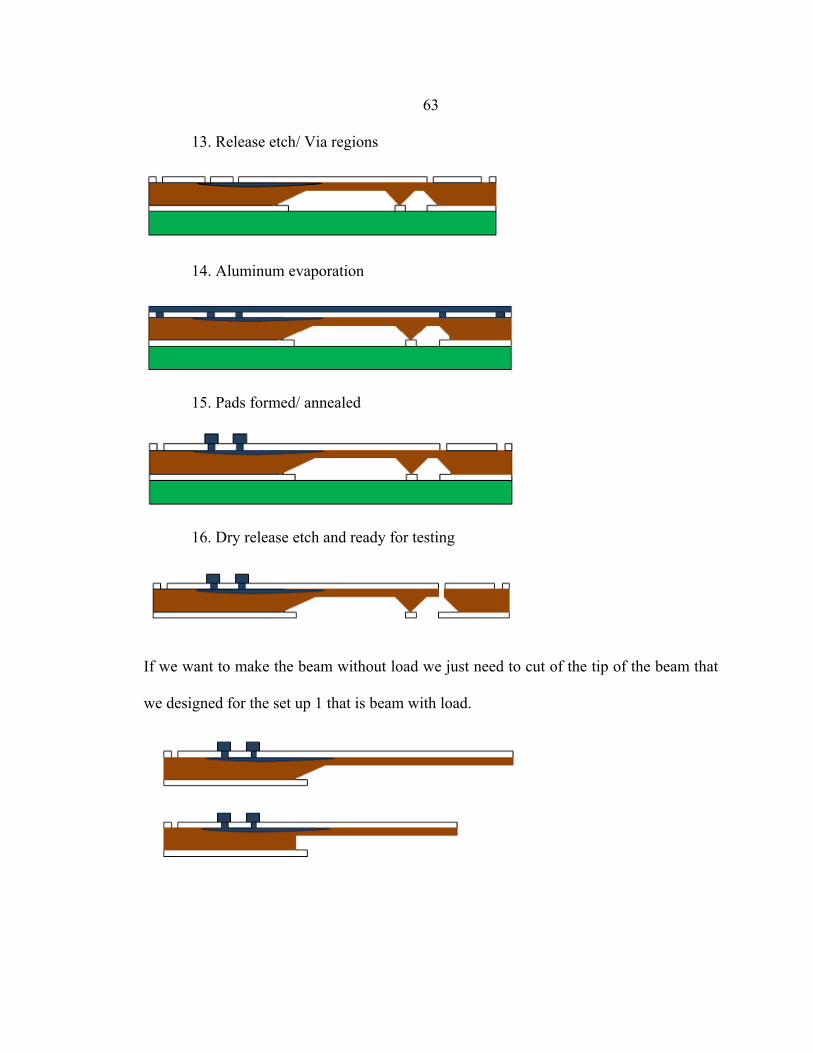
63

13. Release etch/ Via regions

14. Aluminum evaporation

15. Pads formed/ annealed

16. Dry release etch and ready for testing

If we want to make the beam without load we just need to cut of the tip of the beam that

we designed for the set up 1 that is beam with load.

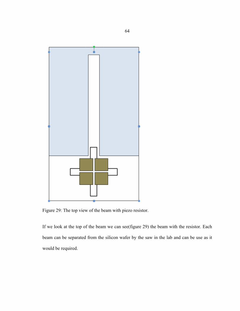
64

Figure 29: The top view of the beam with piezo resistor. If we look at the top of the beam we can see(figure 29) the beam with the resistor. Each

beam can be separated from the silicon wafer by the saw in the lab and can be use as it

would be required.

65

CHAPTER 7

FUTURE WORK AND CONCLUSION

The future work of these consequences will be the fabrication of the beam which

will need the clean room facility. After fabrication steps done test should be done on

different liquids to get the ultimate results.

The results found by the vibrometer and the finite element analysis proves that

miniaturization of the process can be possible by MEMS device to find the rheological

property of the fluids. At a time good knowledge on operating the vibrometer software

also need to compare the final output.

66

REFERENCES

67

1. D. Sparks, R. Smith, V. Cruz, A. Chimbayo, D Riley, N. Najafi, Dynamic and kinematic viscosity measurements with a resonating microtube., Sensors and Actuators A149 (2009) 38-41.

2. C. David , C.L Michael, A.J. Michael, Z. Zhibing, Measurement of Dynamic

Properties of small volumes of liquid using MEMS. 3. S. Raha, et al., Cone and plate rheometer for polymer melts, J. Phys. E: Sci. Instrum.

1 (1968) 1113–1115. 4. K. Nishimura, Viscosity of fluidized snow, Cold Reg. Sci. Technol. 24 (2) (1996)

117–127. 5. S. Feng, A.L. Graham, P.T. Reardon, J. Abbott, L. Mondy, Improving falling ball test

for viscosity determination, J. Fluids Eng. 128 (2006) 157–163. 6. S. Baek, J.J. Magda, Monolithic rheometer plate fabricated using silicon

micromachining technology and containing miniature pressure sensors for N1 and N2 measurements, J. Rheol. 47 (5) (2003) 11–17.

7. A. Buosciolo, G. Pesce, A. Sasso, New calibration method for position detector for

simultaneous measurements of force constants and local viscosity in optical tweezers, Opt. Commun. 230 (4–6) (2004) 357–368.

8. D.M. Curtin, D.T. Newport, M.R. Davies, Utilising _-PIV and pressure

measurements to determine the viscosity of a DNAsolution in a microchannel, Exp. Therm. Fluid Sci. 30 (8) (2006) 843–852.

9. J.J. Crassous, R. R´egisser,M. Ballauff, Characterization of the viscoelastic behaviour

of complex fluids using the piezoelastic axial vibrator, J. Rheol. 49 (4) (2005) 851–863.

10. Lin Y., Lin C., Yang L., Wang A., “Micro-viscometer based on electrowetting on

dielectric’’, Electrochimica Acta 52(2007)2876-2883. 11. Riesch C.,Reichel E. K., keplinger F.,Jakoby B. Charecterizing Vibrating Cantilevers

for Liquid Viscosity and Density Sensing ,Journal of sensors Vol 2008,Article ID[ 697062 ]

12. Stark W.,Burghardt S., Hennemeyer M. Cantilever Micro-rheometer for the

Charecterization of sugar solutions, ISSN 1424-8220,2008 by MDPI 13. Sparks D., Smith R., Cruz V, Tran N., Chimbayo A. , Rilay D.,Najafi N., “dynamic

and kinematic viscosity measurements with a resonating microtube

68

14. Microscope cantilever beams immersed in fluids”, American Institute of Physics. [S0021-8979(00)02007-7]

15. J.W.M. Chon and P. Mulvaney, Rheological measurements using microcantilevers,

2002 by The Society of Rheology, Inc. 16. www.Polytec.com 17. Kaiser Todd, Leone Mall ,MEMS fabrication as a multidisciplinary laboratory , 18. Ahmed N., Nino F.D., Moy V.T., Measurement of solution by atomic force

microscopy, 2001 American Institute of Physics , [DOI : 10. 1063/1.1368856] 19. ANSYS Tutorial 12.1 version.

69

APPENDIX A

ANSYS PROGRAM

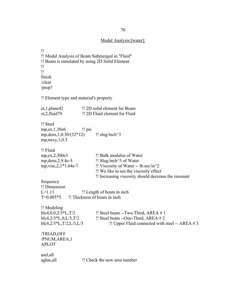
70

Modal Analysis:[water]:

!! !! Modal Analysis of Beam Submerged in "Fluid" !! Beam is simulated by using 2D Solid Element !! !! finish /clear /prep7 !! Element type and material's property et,1,plane42 !! 2D solid element for Beam et,2,fluid79 !! 2D Fluid element for Fluid !! Steel mp,ex,1,30e6 !! psi mp,dens,1,0.30/(32*12) !! slug/inch^3 mp,nuxy,1,0.3 !! Fluid mp,ex,2,300e3 !! Bulk modulus of Water mp,dens,2,9.4e-5 !! Slug/inch^3 of Water mp,visc,2,1*1.64e-7 !! Viscosity of Water -- lb.sec/in^2 !! We like to see the viscosity effect !! Increasing viscosity should decrease the resonant frequency !! Dimension L=1.11 !! Length of beam in inch T=0.005*5 !! Thickness of beam in inch !! Modeling blc4,0,0,2/3*L,T/2 !! Steel beam --Two-Third, AREA # 1 blc4,2/3*L,0,L/3,T/2 !! Steel beam --One-Third, AREA # 2 blc4,2/3*L,T/2,L/3,L/3 !! Upper Fluid connected with steel -- AREA # 3 /TRIAD,OFF /PNUM,AREA,1 APLOT asel,all aglue,all !! Check the new area number

71

!! Mesh control and meshing /pnum,line,1 lplot lsel,s,line,,1,3,2 lesize,all,,,50 lsel,s,line,,13,14,1 lsel,a,line,,11 lesize,all,,,25 lsel,s,line,,2,6,2 lesize,all,,,2 lsel,s,line,,15,16,1 lesize,all,,,25,4 !! Finer Meshing Towards Solid Model !! Meshing Solid mat,1 type,1 asel,s,area,,1,4,3 amesh,all !! Meshing Fluid mat,2 type,2 asel,inve amesh,all asel,all aplot !! Define local coordinate system local,11,0,L,0 csys,11 asel,s,area,,4,5 arsym,x,all asel,all aplot !! CHANGE ELEMENT TYPE FOR FLUID asel,s,area,,2 esla

72

mat,2 type,2 emodify,all !! FULL MODEL BY Y-SYMMETRY asel,all arsym,y,all !! Merging all entities allsel eplot nummrg,all eplot /pnum,line,0 /pnum,area,1 aplot !! SOLID STRUCTURES -- AREA # 1,4,6,9 !! ALL OTHER AREAS -- FLUID !! Boundary condition allsel eplot csys,0 nsel,s,loc,x,0 d,all,all,0 !! Fixed end of the beam /pnum,line,1 /pnum,area,0 lplot eplot /pbc,all,,1 lsel,s,line,,11,12,(12-11) !! Upper Wall lsel,a,line,,27,33,(33-27) !! Lower Wall nsll,,1 d,all,uy,0 lsel,all lplot lsel,s,line,,17 lsel,a,line,,9 !! Right Side Wall lsel,a,line,,25

73

lsel,a,line,,28 nsll,,1 d,all,ux,0 !!lsel,s,line,,15 !! Left Side Wall !!lsel,a,line,,34 !!nsll !!nsel,a,node,,254 !! Upper-Left most node !!nsel,a,node,,2588 !! Lower-Left most node !!d,all,ux,0 !! Assign solid-fluid interaction !! !! I like to assign solid-fluid interaction !! But, Fluid79 does not have that option !! !! Lower fluid elements connected with steel !!allsel !!eplot !!nsel,s,loc,y,-T/2 !!nsel,r,loc,x,2/3*L,L !!esln, !!esel,r,mat,,2 !!esel,u,elem,,1600,1625,(1625-1600) !!sfe,all,1,fsi !! Upper fluid elements connected with steel !!nsel,all !!nplot !!nsel,s,loc,y,T/2 !!nsel,r,loc,x,2/3*L,L !!esln !!esel,r,mat,,2 !!esel,u,elem,,825,850,(850-825) !!sfe,all,1,fsi !! Right Side Fluid Element !!esel,s,elem,,800,825,(825-800) !!sfe,all,4,fsi !!esel,s,elem,,1575,1600,(1600-1575) !!sfe,all,2,fsi !! !! Define Master DOF

74

allsel eplot esel,s,mat,,1 nsle m,all,uy allsel eplot finish Harmonic Analysis[Air]:

!! !! Modal Analysis of Beam Submerged in "Fluid" !! Beam is simulated by using 2D Solid Element !! !! finish /clear /prep7 !! Element type and material's property et,1,plane42 !! 2D solid element for Beam et,2,fluid79 !! 2D Fluid element for Fluid !! Steel mp,ex,1,200e9 !! Pa mp,dens,1,7850 !! kg/m^3 mp,nuxy,1,0.3 !! Fluid mp,ex,2,1.42*e5 !! Bulk modulus of Air, Pa mp,dens,2,(1-0)*1.1933 !! Density of air, kg/m^3 mp,visc,2,2.075*1.0e-5 !! Viscosity of air,Pa-sec (N.s/m^2) !! 1 Poise = 0.1 Pa-sec. !! We like to see the viscosity effect !! Increasing viscosity should decrease the resonant frequency !! Dimension L=0.0282 !! L=1.11 inch = 0.0282 m T=0.000127*1 !! T= 0.005 inch = 0.000127 m

75

!! Modeling blc4,0,0,2/3*L,T/2 !! Steel beam --Two-Third, AREA # 1 blc4,2/3*L,0,L/3,T/2 !! Steel beam --One-Third, AREA # 2 blc4,2/3*L,T/2,L/3,L/3 !! Upper Fluid connected with steel -- AREA # 3 /TRIAD,OFF /PNUM,AREA,1 APLOT asel,all aglue,all !! Check the new area number !! Mesh control and meshing /pnum,line,1 lplot lsel,s,line,,1,3,2 lesize,all,,,100 lsel,s,line,,13,14,1 lsel,a,line,,11 lesize,all,,,50 lsel,s,line,,2,6,2 lesize,all,,,2 lsel,s,line,,15,16,1 lesize,all,,,50,5 !! No Finer Meshing Towards Solid Model !! Meshing Solid mat,1 type,1 asel,s,area,,1,4,3 amesh,all !! Meshing Fluid mat,2 type,2 asel,inve amesh,all asel,all aplot

76

eplot !! Define local coordinate system local,11,0,L,0 csys,11 asel,s,area,,4,5 arsym,x,all asel,all aplot !! CHANGE ELEMENT TYPE FOR FLUID asel,s,area,,2 esla mat,2 type,2 emodify,all !! FULL MODEL BY Y-SYMMETRY asel,all arsym,y,all !! Merging all entities allsel eplot nummrg,all,1e-6 eplot /pnum,line,0 /pnum,area,1 aplot !! SOLID STRUCTURES -- AREA # 1,4,6,9 !! ALL OTHER AREAS -- FLUID !! Boundary condition allsel eplot csys,0 nsel,s,loc,x,0 d,all,all,0 !! Fixed end of the beam /pnum,line,1 /pnum,area,0

77

lplot lsel,s,line,,11,12,(12-11) !! Upper Wall lsel,a,line,,27,33,(33-27) !! Lower Wall nsll,,1 d,all,uy,0 lsel,all lplot lsel,s,line,,17 lsel,a,line,,9 !! Right Side Wall lsel,a,line,,25 lsel,a,line,,28 nsll,,1 d,all,ux,0 !! Define Master DOF !! This is important for REDUCED Eigen Solver allsel eplot esel,s,mat,,1 nsle m,all,uy allsel eplot finish !! Modal Analysis /solution antype, harmic f,304,fy,0.1 harfrq,0,200 nsubst,100 kbc,1 outres,nsol,1 solve finish /post26 nsol,2,304,u,y plvar,2 prvar,2 finish

78

Harmonic Analysis[Water] !! !! Modal Analysis of Beam Submerged in "Fluid" !! Beam is simulated by using 2D Solid Element !! !! finish /clear /prep7 !! Element type and material's property et,1,plane42 !! 2D solid element for Beam et,2,fluid79 !! 2D Fluid element for Fluid !! Steel mp,ex,1,200e9 !! Pa mp,dens,1,7850 !! kg/m^3 mp,nuxy,1,0.3 !! Fluid mp,ex,2,2.15e9 !! Bulk modulus of Water, Pa mp,dens,2,(1-0)*1000 !! Density of Water, kg/m^3 mp,visc,2,658*1.0e-5 !! Viscosity of Water,Pa-sec (N.s/m^2) !! 1 Poise = 0.1 Pa-sec. !! We like to see the viscosity effect !! Increasing viscosity should decrease the resonant frequency !! Dimension L=0.0282 !! L=1.11 inch = 0.0282 m T=0.000127*1 !! T= 0.005 inch = 0.000127 m !! Modeling blc4,0,0,2/3*L,T/2 !! Steel beam --Two-Third, AREA # 1 blc4,2/3*L,0,L/3,T/2 !! Steel beam --One-Third, AREA # 2 blc4,2/3*L,T/2,L/3,L/3 !! Upper Fluid connected with steel -- AREA # 3 /TRIAD,OFF /PNUM,AREA,1 APLOT asel,all aglue,all !! Check the new area number

79

!! Mesh control and meshing /pnum,line,1 lplot lsel,s,line,,1,3,2 lesize,all,,,100 lsel,s,line,,13,14,1 lsel,a,line,,11 lesize,all,,,50 lsel,s,line,,2,6,2 lesize,all,,,2 lsel,s,line,,15,16,1 lesize,all,,,50,5 !! No Finer Meshing Towards Solid Model !! Meshing Solid mat,1 type,1 asel,s,area,,1,4,3 amesh,all !! Meshing Fluid mat,2 type,2 asel,inve amesh,all asel,all aplot eplot !! Define local coordinate system local,11,0,L,0 csys,11 asel,s,area,,4,5 arsym,x,all asel,all aplot !! CHANGE ELEMENT TYPE FOR FLUID asel,s,area,,2

80

esla mat,2 type,2 emodify,all !! FULL MODEL BY Y-SYMMETRY asel,all arsym,y,all !! Merging all entities allsel eplot nummrg,all,1e-6 eplot /pnum,line,0 /pnum,area,1 aplot !! SOLID STRUCTURES -- AREA # 1,4,6,9 !! ALL OTHER AREAS -- FLUID !! Boundary condition allsel eplot csys,0 nsel,s,loc,x,0 d,all,all,0 !! Fixed end of the beam /pnum,line,1 /pnum,area,0 lplot lsel,s,line,,11,12,(12-11) !! Upper Wall lsel,a,line,,27,33,(33-27) !! Lower Wall nsll,,1 d,all,uy,0 lsel,all lplot lsel,s,line,,17 lsel,a,line,,9 !! Right Side Wall lsel,a,line,,25 lsel,a,line,,28

81

nsll,,1 d,all,ux,0 !! Define Master DOF !! This is important for REDUCED Eigen Solver allsel eplot esel,s,mat,,1 nsle m,all,uy allsel eplot finish !! Modal Analysis /solution antype,harmic f,304,fy,0.1 harfrq,0,200 nsubst,100 kbc,1 outres,nsol,1 solve finish /post26 nsol,2,304,u,y plvar,2 prvar,2 finish Harmonic Analysis [DTE24] !! !! Modal Analysis of Beam Submerged in "Fluid" !! Beam is simulated by using 2D Solid Element !! !! finish /clear /prep7 !! Element type and material's property

82

et,1,plane42 !! 2D solid element for Beam et,2,fluid79 !! 2D Fluid element for Fluid !! Steel mp,ex,1,200e9 !! Pa mp,dens,1,7850 !! kg/m^3 mp,nuxy,1,0.3 !! Fluid mp,ex,2,1.03421e9 !! Bulk modulus of DTE24, Pa mp,dens,2,(1-0)*871 !! Density of DTE24, kg/m^3 mp,visc,2,274.365*1.0e-4 !! Viscosity of DTE24,Pa-sec (N.s/m^2) !! 1 Poise = 0.1 Pa-sec. !! We like to see the viscosity effect !! Increasing viscosity should decrease the resonant frequency !! Dimension L=0.0282 !! L=1.11 inch = 0.0282 m T=0.000127*1 !! T= 0.005 inch = 0.000127 m !! Modeling blc4,0,0,2/3*L,T/2 !! Steel beam --Two-Third, AREA # 1 blc4,2/3*L,0,L/3,T/2 !! Steel beam --One-Third, AREA # 2 blc4,2/3*L,T/2,L/3,L/3 !! Upper Fluid connected with steel -- AREA # 3 /TRIAD,OFF /PNUM,AREA,1 APLOT asel,all aglue,all !! Check the new area number !! Mesh control and meshing /pnum,line,1 lplot lsel,s,line,,1,3,2 lesize,all,,,100 lsel,s,line,,13,14,1 lsel,a,line,,11 lesize,all,,,50 lsel,s,line,,2,6,2

83

lesize,all,,,2 lsel,s,line,,15,16,1 lesize,all,,,50,5 !! No Finer Meshing Towards Solid Model !! Meshing Solid mat,1 type,1 asel,s,area,,1,4,3 amesh,all !! Meshing Fluid mat,2 type,2 asel,inve amesh,all asel,all aplot eplot !! Define local coordinate system local,11,0,L,0 csys,11 asel,s,area,,4,5 arsym,x,all asel,all aplot !! CHANGE ELEMENT TYPE FOR FLUID asel,s,area,,2 esla mat,2 type,2 emodify,all !! FULL MODEL BY Y-SYMMETRY asel,all arsym,y,all !! Merging all entities allsel eplot

84

nummrg,all,1e-6 eplot /pnum,line,0 /pnum,area,1 aplot !! SOLID STRUCTURES -- AREA # 1,4,6,9 !! ALL OTHER AREAS -- FLUID !! Boundary condition allsel eplot csys,0 nsel,s,loc,x,0 d,all,all,0 !! Fixed end of the beam /pnum,line,1 /pnum,area,0 lplot lsel,s,line,,11,12,(12-11) !! Upper Wall lsel,a,line,,27,33,(33-27) !! Lower Wall nsll,,1 d,all,uy,0 lsel,all lplot lsel,s,line,,17 lsel,a,line,,9 !! Right Side Wall lsel,a,line,,25 lsel,a,line,,28 nsll,,1 d,all,ux,0 !! Define Master DOF !! This is important for REDUCED Eigen Solver allsel eplot esel,s,mat,,1 nsle m,all,uy allsel eplot

85

finish !! Modal Analysis /solution antype,harmic f,304,fy,0.1 harfrq,0,200 nsubst,100 kbc,1 outres,nsol,1 solve finish /post26 nsol,2,304,u,y plvar,2 prvar,2 finish Harmonic Analysis [DTE25] !! !! Modal Analysis of Beam Submerged in "Fluid" !! Beam is simulated by using 2D Solid Element !! !! finish /clear /prep7 !! Element type and material's property et,1,plane42 !! 2D solid element for Beam et,2,fluid79 !! 2D Fluid element for Fluid !! Steel mp,ex,1,200e9 !! Pa mp,dens,1,7850 !! kg/m^3 mp,nuxy,1,0.3 !! Fluid mp,ex,2,.106868733e9 !! Bulk modulus of DTE25, Pa mp,dens,2,(1-0)*876 !! Density of Water, kg/m^3 mp,visc,2,387.192*1.0e-4 !! Viscosity of DTE25,Pa-sec (N.s/m^2)

86

!! 1 Poise = 0.1 Pa-sec. !! We like to see the viscosity effect !! Increasing viscosity should decrease the resonant frequency !! Dimension L=0.0282 !! L=1.11 inch = 0.0282 m T=0.000127*1 !! T= 0.005 inch = 0.000127 m !! Modeling blc4,0,0,2/3*L,T/2 !! Steel beam --Two-Third, AREA # 1 blc4,2/3*L,0,L/3,T/2 !! Steel beam --One-Third, AREA # 2 blc4,2/3*L,T/2,L/3,L/3 !! Upper Fluid connected with steel -- AREA # 3 /TRIAD,OFF /PNUM,AREA,1 APLOT asel,all aglue,all !! Check the new area number !! Mesh control and meshing /pnum,line,1 lplot lsel,s,line,,1,3,2 lesize,all,,,100 lsel,s,line,,13,14,1 lsel,a,line,,11 lesize,all,,,50 lsel,s,line,,2,6,2 lesize,all,,,2 lsel,s,line,,15,16,1 lesize,all,,,50,5 !! No Finer Meshing Towards Solid Model !! Meshing Solid mat,1 type,1 asel,s,area,,1,4,3 amesh,all !! Meshing Fluid

87

mat,2 type,2 asel,inve amesh,all asel,all aplot eplot !! Define local coordinate system local,11,0,L,0 csys,11 asel,s,area,,4,5 arsym,x,all asel,all aplot !! CHANGE ELEMENT TYPE FOR FLUID asel,s,area,,2 esla mat,2 type,2 emodify,all !! FULL MODEL BY Y-SYMMETRY asel,all arsym,y,all !! Merging all entities allsel eplot nummrg,all,1e-6 eplot /pnum,line,0 /pnum,area,1 aplot !! SOLID STRUCTURES -- AREA # 1,4,6,9 !! ALL OTHER AREAS -- FLUID !! Boundary condition allsel

88

eplot csys,0 nsel,s,loc,x,0 d,all,all,0 !! Fixed end of the beam /pnum,line,1 /pnum,area,0 lplot lsel,s,line,,11,12,(12-11) !! Upper Wall lsel,a,line,,27,33,(33-27) !! Lower Wall nsll,,1 d,all,uy,0 lsel,all lplot lsel,s,line,,17 lsel,a,line,,9 !! Right Side Wall lsel,a,line,,25 lsel,a,line,,28 nsll,,1 d,all,ux,0 !! Define Master DOF !! This is important for REDUCED Eigen Solver allsel eplot esel,s,mat,,1 nsle m,all,uy allsel eplot finish !! Modal Analysis /solution antype,harmic f,304,fy,0.1 harfrq,0,200 nsubst,100 kbc,1 outres,nsol,1 solve finish

89

/post26 nsol,2,304,u,y plvar,2 prvar,2 finish Harmonic Analysis[DTE 26] !! !! Modal Analysis of Beam Submerged in "Fluid" !! Beam is simulated by using 2D Solid Element !! !! finish /clear /prep7 !! Element type and material's property et,1,plane42 !! 2D solid element for Beam et,2,fluid79 !! 2D Fluid element for Fluid !! Steel mp,ex,1,200e9 !! Pa mp,dens,1,7850 !! kg/m^3 mp,nuxy,1,0.3 !! Fluid mp,ex,2,.110316112e9 !! Bulk modulus of DTE26, Pa mp,dens,2,(1-0)*886 !! Density of DTe26, kg/m^3 mp,visc,2,632.604*1.0e-4 !! Viscosity of Water,Pa-sec (N.s/m^2) !! 1 Poise = 0.1 Pa-sec. !! We like to see the viscosity effect !! Increasing viscosity should decrease the resonant frequency !! Dimension L=0.0282 !! L=1.11 inch = 0.0282 m T=0.000127*1 !! T= 0.005 inch = 0.000127 m !! Modeling blc4,0,0,2/3*L,T/2 !! Steel beam --Two-Third, AREA # 1 blc4,2/3*L,0,L/3,T/2 !! Steel beam --One-Third, AREA # 2

90

blc4,2/3*L,T/2,L/3,L/3 !! Upper Fluid connected with steel -- AREA # 3 /TRIAD,OFF /PNUM,AREA,1 APLOT asel,all aglue,all !! Check the new area number !! Mesh control and meshing /pnum,line,1 lplot lsel,s,line,,1,3,2 lesize,all,,,100 lsel,s,line,,13,14,1 lsel,a,line,,11 lesize,all,,,50 lsel,s,line,,2,6,2 lesize,all,,,2 lsel,s,line,,15,16,1 lesize,all,,,50,5 !! No Finer Meshing Towards Solid Model !! Meshing Solid mat,1 type,1 asel,s,area,,1,4,3 amesh,all !! Meshing Fluid mat,2 type,2 asel,inve amesh,all asel,all aplot eplot !! Define local coordinate system local,11,0,L,0 csys,11

91

asel,s,area,,4,5 arsym,x,all asel,all aplot !! CHANGE ELEMENT TYPE FOR FLUID asel,s,area,,2 esla mat,2 type,2 emodify,all !! FULL MODEL BY Y-SYMMETRY asel,all arsym,y,all !! Merging all entities allsel eplot nummrg,all,1e-6 eplot /pnum,line,0 /pnum,area,1 aplot !! SOLID STRUCTURES -- AREA # 1,4,6,9 !! ALL OTHER AREAS -- FLUID !! Boundary condition allsel eplot csys,0 nsel,s,loc,x,0 d,all,all,0 !! Fixed end of the beam /pnum,line,1 /pnum,area,0 lplot lsel,s,line,,11,12,(12-11) !! Upper Wall lsel,a,line,,27,33,(33-27) !! Lower Wall nsll,,1

92

d,all,uy,0 lsel,all lplot lsel,s,line,,17 lsel,a,line,,9 !! Right Side Wall lsel,a,line,,25 lsel,a,line,,28 nsll,,1 d,all,ux,0 !! Define Master DOF !! This is important for REDUCED Eigen Solver allsel eplot esel,s,mat,,1 nsle m,all,uy allsel eplot finish !! Modal Analysis /solution antype,harmic f,304,fy,0.1 harfrq,0,200 nsubst,100 kbc,1 outres,nsol,1 solve finish /post26 nsol,2,304,u,y plvar,2 prvar,2 finish Modal analysis [water] !! !! Modal Analysis of Beam Submerged in "Fluid" !! Beam is simulated by using 2D Solid Element

93

!! !! finish /clear /prep7 !! Element type and material's property et,1,plane42 !! 2D solid element for Beam et,2,fluid79 !! 2D Fluid element for Fluid !! Steel mp,ex,1,200e9 !! Pa mp,dens,1,7850 !! kg/m^3 mp,nuxy,1,0.3 !! Fluid mp,ex,2,2.15e9 !! Bulk modulus of Water, Pa mp,dens,2,(1-0)*1000 !! Density of Water, kg/m^3 mp,visc,2,658*1.0e-5 !! Viscosity of Water,Pa-sec (N.s/m^2) !! 1 Poise = 0.1 Pa-sec. !! We like to see the viscosity effect !! Increasing viscosity should decrease the resonant frequency !! Dimension L=0.0282 !! L=1.11 inch = 0.0282 m T=0.000127*1 !! T= 0.005 inch = 0.000127 m !! Modeling blc4,0,0,2/3*L,T/2 !! Steel beam --Two-Third, AREA # 1 blc4,2/3*L,0,L/3,T/2 !! Steel beam --One-Third, AREA # 2 blc4,2/3*L,T/2,L/3,L/3 !! Upper Fluid connected with steel -- AREA # 3 /TRIAD,OFF /PNUM,AREA,1 APLOT asel,all aglue,all !! Check the new area number !! Mesh control and meshing /pnum,line,1 lplot

94

lsel,s,line,,1,3,2 lesize,all,,,100 lsel,s,line,,13,14,1 lsel,a,line,,11 lesize,all,,,50 lsel,s,line,,2,6,2 lesize,all,,,2 lsel,s,line,,15,16,1 lesize,all,,,50,5 !! No Finer Meshing Towards Solid Model !! Meshing Solid mat,1 type,1 asel,s,area,,1,4,3 amesh,all !! Meshing Fluid mat,2 type,2 asel,inve amesh,all asel,all aplot eplot !! Define local coordinate system local,11,0,L,0 csys,11 asel,s,area,,4,5 arsym,x,all asel,all aplot !! CHANGE ELEMENT TYPE FOR FLUID asel,s,area,,2 esla mat,2 type,2

95

emodify,all !! FULL MODEL BY Y-SYMMETRY asel,all arsym,y,all !! Merging all entities allsel eplot nummrg,all,1e-6 eplot /pnum,line,0 /pnum,area,1 aplot !! SOLID STRUCTURES -- AREA # 1,4,6,9 !! ALL OTHER AREAS -- FLUID !! Boundary condition allsel eplot csys,0 nsel,s,loc,x,0 d,all,all,0 !! Fixed end of the beam /pnum,line,1 /pnum,area,0 lplot lsel,s,line,,11,12,(12-11) !! Upper Wall lsel,a,line,,27,33,(33-27) !! Lower Wall nsll,,1 d,all,uy,0 lsel,all lplot lsel,s,line,,17 lsel,a,line,,9 !! Right Side Wall lsel,a,line,,25 lsel,a,line,,28 nsll,,1 d,all,ux,0

96

!! Define Master DOF !! This is important for REDUCED Eigen Solver allsel eplot esel,s,mat,,1 nsle m,all,uy allsel eplot finish !! Modal Analysis /solution antype,modal !!modopt,reduc,5,0,4000 !! Element Fluid79 supports only "Reduced" Modal Option modopt,damp,20,10,500 !!modop,qrdamp,10,20,,on mxpand,,0,100,yes solve finish