Dis cus si on Paper No. 17-017

Dynamic Scoring of Tax Reforms in the European Union

Salvador Barrios, Mathias Dolls, Anamaria Maftei, Andreas Peichl, Sara Riscado,

Janos Varga, and Christian Wittneben

Dis cus si on Paper No. 17-017

Dynamic Scoring of Tax Reforms in the European Union

Salvador Barrios, Mathias Dolls, Anamaria Maftei, Andreas Peichl, Sara Riscado,

Janos Varga, and Christian Wittneben

Download this ZEW Discussion Paper from our ftp server:

http://ftp.zew.de/pub/zew-docs/dp/dp17017.pdf

Die Dis cus si on Pape rs die nen einer mög lichst schnel len Ver brei tung von neue ren For schungs arbei ten des ZEW. Die Bei trä ge lie gen in allei ni ger Ver ant wor tung

der Auto ren und stel len nicht not wen di ger wei se die Mei nung des ZEW dar.

Dis cus si on Papers are inten ded to make results of ZEW research prompt ly avai la ble to other eco no mists in order to encou ra ge dis cus si on and sug gesti ons for revi si ons. The aut hors are sole ly

respon si ble for the con tents which do not neces sa ri ly repre sent the opi ni on of the ZEW.

 

1  

Dynamic scoring of tax reforms in the European Union1 

Salvador Barrios, Mathias Dolls, Anamaria Maftei, Andreas Peichl, Sara Riscado, Janos Varga 

and Christian Wittneben 

 

Abstract 

In  this paper, we present  the  first dynamic  scoring exercise  linking a multi‐country microsimulation 

and  DSGE models  for  all  countries  of  the  European  Union. We  illustrate  our  novel methodology 

analysing a hypothetical tax reform for Belgium. We then evaluate real tax reforms in Italy and Poland. 

Our approach takes into account the feedback effects resulting from adjustments in the labor market 

and the economy‐wide reaction to the tax policy changes. Our results suggest that accounting for the 

behavioral  reaction  and macroeconomic  feedback  to  tax  policy  changes  enriches  the  tax  reforms' 

analysis, by increasing the accuracy of the direct fiscal and distributional impact assessment provided 

by  the microsimulation model  for  the  tax  reforms  considered. Our  results are  in  line with previous 

dynamic scoring exercises, showing that most tax reforms entail relatively smaller feedback effects in 

terms of the  labor tax revenues for tax cuts benefiting workers, compared with the ones granted to 

firms. 

  

   

                                                            1 Contact author:  Salvador Barrios, European Commission,  Joint Research Centre  (JRC),  Fiscal Policy Analysis Unit,  c/  Inca Garcilaso 3, E‐41092 Sevilla, salvador.barrios@ec.europa.eu, https://ec.europa.eu/jrc/en/person/salvador‐barrios. The views expressed are purely those of the authors and may not in any circumstances be regarded as stating an official position of the European Commission.  

 

2  

Acknowledgments  

We are  thankful  for  the valuable comments of  the participants of  the APPAM Fall Conference 2016 

and  the  pre‐APPAM  conference  organised  by  the  Urban  Institute  in Washington  DC. We  are  also 

thankful  to  Douglas  Holtz‐Eakin,  Salvador  Espinosa,  Athena  Kalyva,  Savina  Princen,  Adriana  Reut, 

Viginta Ivaskaite‐Tamosiune and Wouter van der Wielen for their helpful insights. 

 

   

 

3  

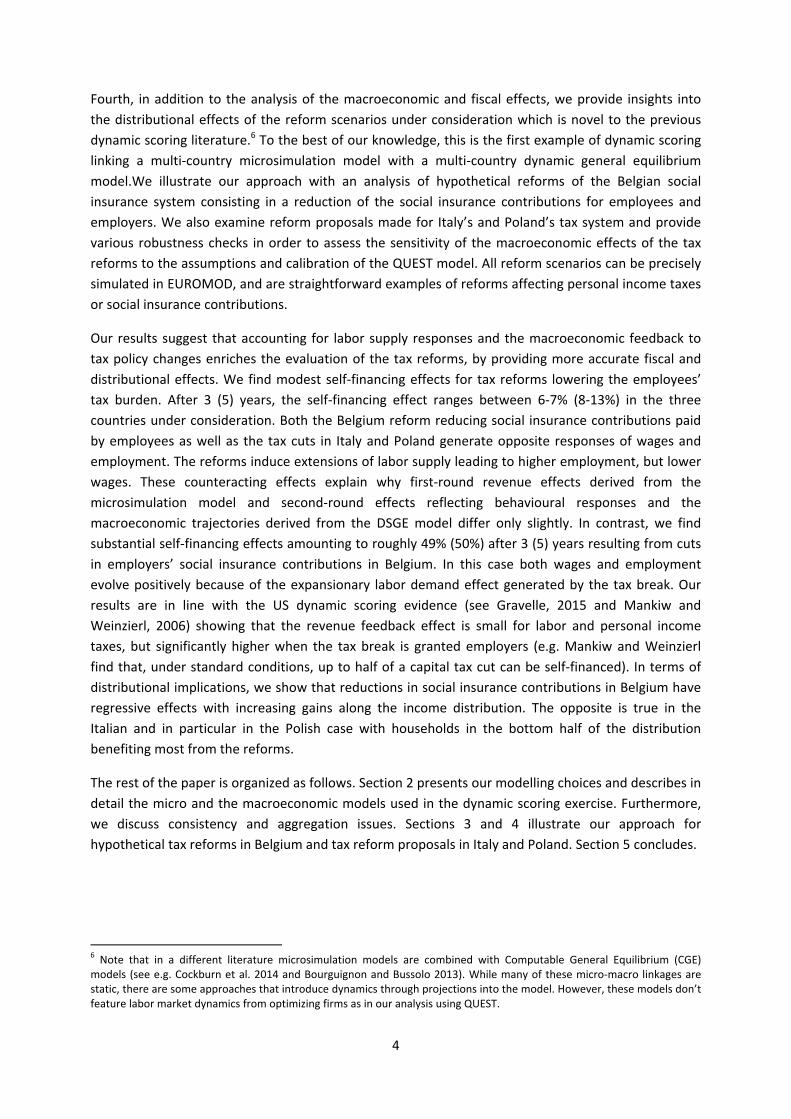
1. Introduction Assessing  the  revenue, behavioral and macroeconomic effects of  tax  reform proposals before  their 

introduction provides  important  information  to  feed  the political and public debate. The  interaction 

between  tax  reforms and  changes  induced  in  the economy are multi‐faceted and  it  is necessary  to 

capture not only the reaction of economic agents  to the tax reforms  (in particular  labor adjustment 

effects), but also the overall economic effect,  including  in the product and factor markets.2 Dynamic 

scoring  techniques provide a useful  tool  for  such analyses.  In  the US, dynamic  scoring analyses are 

now  well  established  and  legally  required  before  significant  changes  in  tax  legislation  are 

implemented.3  In contrast  to  the US, dynamic scoring has not been applied  in  the  fiscal governance 

framework in the European Union (EU) so far. Yet, such analysis would allow an in‐depth evaluation of 

discretionary  tax measures  and  a  better  assessment  of  the  true  fiscal  policy  stance which  remain 

important  issues  in the EU (Buti and Van den Noord, 2004). Moreover,  in a policy context where the 

European  Commission  analyses  the  fiscal  and  structural  reform  policies  of  every Member  State  – 

providing  recommendations, and monitoring  their  implementation according  to an annual  round of 

policy dialogue (the so‐called European Semester) – the analysis of how fiscal and structural reforms 

can affect national budgets as well as Member States´ economic performance is required.4 Accounting 

for  macroeconomic  feedback  effects  of  tax  reforms  is  also  crucial  for  the  determination  of  the 

cyclically  adjusted  fiscal  balance which  plays  a  key  role  in  the  European  fiscal  framework  (see  in 

particular Larch and Turrini, 2010). 

In  this paper we develop a dynamic  scoring  framework  for modelling and analysing  tax and benefit 

reforms. A key feature of our dynamic scoring approach is to combine EUROMOD, the microsimulation 

model for all European Union Member States, with QUEST, the European Commission’s DSGE model 

used  for  the  analysis  of  structural  reforms  (including  fiscal  reforms).5  We  demonstrate  our 

methodology  and  show  that  the  use  of  EUROMOD  enriches  the  analysis  of  fiscal  reforms  in many 

respects.  First,  it  allows  for  a  precise  translation  of  actual  tax  reform measures  into  policy  shocks 

which is not possible using macroeconomic models alone that only differentiate between capital and 

labor  taxes  (see e.g. Mankiw and Weinzierl 2006,  Leeper and Yang 2008, Trabandt and Uhlig 2011, 

Strulik and Trimborn 2012). EUROMOD contains all relevant rules of the tax‐benefit systems in the EU 

Member  States  and  allows  for  the  simulation  of  direct  taxes  and  benefits  according  to  actual 

legislation and hypothetical reform scenarios. Second, we augment EUROMOD with a discrete choice 

labor supply model in order to account for labor responses to the tax reforms. Third, microsimulation 

models  alone  tend  to  ignore  how  tax  reforms  endogenously  affect  prices  and  volumes  as well  as 

monetary and fiscal variables in the economy that can lead to non‐negligible second‐round effects on 

tax‐revenues.  These  effects  can  be  consistently modelled  in  dynamic  general  equilibrium models. 

                                                            2 See Adam and Bozio 2009 for a comprehensive assessment of the dynamic scoring exercise. 3 In the US, dynamic scoring analyses are conducted by the Joint Committee on Taxation (JCT) and the Congressional Budget Office (CBO). The JCT has been responsible for a macroeconomic impact analysis of changes in tax law since 2003. In addition, the  CBO  has  incorporated  these macroeconomic  feedback  effects  into  their  estimates  of  fiscal  effects  if  revenue  effects exceeded $5 billion  in any fiscal year. Since 2015, the JCT and the CBO are obliged to provide precise estimates for output and  revenue  feedback  effects of major  tax  and mandatory  spending  changes  (see Altshuler  et  al.  2005, Auerbach  2005, Furman 2006, Gravelle 2014, 2015 and Holtz‐Eakin 2015 for more details). 4 For example, recently the European Commission has also started to collect data on estimates of the impact of discretionary tax measures relying on the Member States' own assessment and providing information at a more disaggregated level (see in particular Barrios and Fargnoli, 2010). 5  See  Sutherland  (2001) and  Sutherland and Figari  (2013)  for a description of  the EUROMOD microsimulation model and Ratto et al. (2009) for details on the QUEST III model. 

 

4  

Fourth,  in addition  to  the analysis of  the macroeconomic and  fiscal effects, we provide  insights  into 

the distributional effects of the reform scenarios under consideration which  is novel to the previous 

dynamic scoring literature.6 To the best of our knowledge, this is the first example of dynamic scoring 

linking  a  multi‐country  microsimulation  model  with  a  multi‐country  dynamic  general  equilibrium 

model.We  illustrate  our  approach  with  an  analysis  of  hypothetical  reforms  of  the  Belgian  social 

insurance  system  consisting  in a  reduction of  the  social  insurance  contributions  for employees and 

employers. We also examine reform proposals made for  Italy’s and Poland’s tax system and provide 

various robustness checks  in order  to assess  the sensitivity of  the macroeconomic effects of  the  tax 

reforms to the assumptions and calibration of the QUEST model. All reform scenarios can be precisely 

simulated in EUROMOD, and are straightforward examples of reforms affecting personal income taxes 

or social insurance contributions.  

Our results suggest  that accounting  for  labor supply responses and  the macroeconomic  feedback  to 

tax policy changes enriches the evaluation of the tax reforms, by providing more accurate  fiscal and 

distributional effects. We  find modest self‐financing effects  for tax reforms  lowering the employees’ 

tax  burden.  After  3  (5)  years,  the  self‐financing  effect  ranges  between  6‐7%  (8‐13%)  in  the  three 

countries under consideration. Both the Belgium reform reducing social  insurance contributions paid 

by employees as well as  the  tax cuts  in  Italy and Poland generate opposite responses of wages and 

employment. The reforms induce extensions of labor supply leading to higher employment, but lower 

wages.  These  counteracting  effects  explain  why  first‐round  revenue  effects  derived  from  the 

microsimulation  model  and  second‐round  effects  reflecting  behavioural  responses  and  the 

macroeconomic  trajectories  derived  from  the DSGE model  differ  only  slightly.  In  contrast, we  find 

substantial self‐financing effects amounting to roughly 49% (50%) after 3 (5) years resulting from cuts 

in  employers’  social  insurance  contributions  in  Belgium.  In  this  case  both wages  and  employment 

evolve positively because of  the expansionary  labor demand effect generated by  the  tax break. Our 

results  are  in  line  with  the  US  dynamic  scoring  evidence  (see  Gravelle,  2015  and  Mankiw  and 

Weinzierl,  2006)  showing  that  the  revenue  feedback  effect  is  small  for  labor  and  personal  income 

taxes, but  significantly higher when  the  tax break  is granted employers  (e.g. Mankiw and Weinzierl 

find that, under standard conditions, up to half of a capital tax cut can be self‐financed).  In terms of 

distributional implications, we show that reductions in social insurance contributions in Belgium have 

regressive  effects with  increasing  gains  along  the  income  distribution.  The  opposite  is  true  in  the 

Italian  and  in  particular  in  the  Polish  case with  households  in  the  bottom  half  of  the  distribution 

benefiting most from the reforms. 

The rest of the paper is organized as follows. Section 2 presents our modelling choices and describes in 

detail the micro and the macroeconomic models used  in the dynamic scoring exercise. Furthermore, 

we  discuss  consistency  and  aggregation  issues.  Sections  3  and  4  illustrate  our  approach  for 

hypothetical tax reforms in Belgium and tax reform proposals in Italy and Poland. Section 5 concludes. 

                                                            6  Note  that  in  a  different  literature microsimulation models  are  combined with  Computable  General  Equilibrium  (CGE) models (see e.g. Cockburn et al. 2014 and Bourguignon and Bussolo 2013). While many of these micro‐macro  linkages are static, there are some approaches that introduce dynamics through projections into the model. However, these models don’t feature labor market dynamics from optimizing firms as in our analysis using QUEST. 

 

5  

2. Modelling second‐round effects of tax reforms In this section, we first present an overview the methodological steps of the dynamic scoring exercise. 

Afterwards, we describe  individually  the different models  involved  in  the exercise  (Appendix A and 

Appendix B provide  further  information on  the discrete  choice  labor  supply model  and on QUEST, 

respectively). Finally, we discuss aggregation issues arising from linking the micro and macro models. 

 

2.1. Methodological framework The methodological steps followed in our dynamic scoring exercise are summarized in Figure 1. 

Figure 1. Methodological steps 

 

As shown in Figure 1, the first step our analysis consists in running EUROMOD for the baseline, i.e. for 

the  actual  tax‐benefit  system,  and  the  reform  scenarios.  This  is  done  to  obtain  the  change  in  the 

implicit tax rates for employees and employers. In addition, we estimate a discrete choice labor supply 

model following the approach by Bargain et al. (2014) in order to derive labor supply elasticities.  

In the second step, the macroeconomic analysis of the tax reforms is conducted by simulating the tax 

reforms in QUEST. For that purpose, QUEST is calibrated using the implicit tax rates and various labor 

market parameters (gross wages,  labor supply elasticities, non‐participation rate) from the first step. 

After  introducing  the policy  shocks on  the  implicit average  tax  rates, we  run  the model  in order  to 

obtain the three years trajectories for the price level, employment and gross wages. Importantly, the 

macroeconomic  projections  from  QUEST  account  for  the  behavioral  reaction  of  firms  (i.e.  labor 

demand) which is missing from typical microsimulation models.  

In a third step, we study the fiscal and distributional effects of the tax reforms by imputing the macro 

projections obtained  in  the  second  step  into EUROMOD. This  includes  setting EUROMOD’s uprating 

factors for prices7 and wages by skills according to the QUEST trajectories for the next three years. In 

addition, the weights of the employed and the rest of the population  in the micro‐data  input file are 

adjusted in order to match the change in the employment variable in QUEST.  

                                                            7  In  EUROMOD  the monetary  variables  are  in  nominal  terms,  so we  need  to  take  into  account  the  evolution  of  prices whenever the year of the policy system does not coincide with the reference year of the survey. 

 

6  

 

2.2 The labor supply discrete choice model Our labor supply model is based on the assumption that households maximize utility and thereby face 

the standard consumption‐leisure trade‐off. In contrast to the classical “continuous choice” approach, 

we  estimate  a  discrete  choice model where  agents  face  a  discrete  set  of  alternatives  in  terms  of 

working hours. Individuals can choose to work zero hours, part‐time (20 hours), full‐time (40 hours) or 

over‐time  (60  hours)  so  that  the  choice  covers  both  the  extensive  and  intensive  margin.8 

Econometrically,  our methodology  entails  the  specification  and  estimation  of  consumption‐leisure 

preferences,  and  the  evaluation  of  utility  at  each  discrete  alternative.9  Utility  consists  of  a 

deterministic part which  is  a  function of observable  variables, and  an error  term which  can  reflect 

optimization  errors of  the household, measurement  error  concerning  the  explanatory  variables, or 

unobserved preference  characteristics.  For  the deterministic part, we  specify  a utility  function  that 

depends  on  both  household  characteristics  and  characteristics  of  the  hours  category,  i.e.  the 

associated work and leisure times and the disposable income from working the respective amount of 

time,  but  also  fixed  costs  of  taking  up work.  By  letting  household  characteristics  enter  the  utility 

function, we allow  for observed heterogeneity  in household preferences. Household  characteristics 

also  influence how gross  income translates  into disposable  income through the tax‐benefit‐function: 

disposable  income  is  a  function  of  household  earnings,  non‐labor  income,  and  household 

characteristics (e.g. age, marital status, number of children). For identification, we exploit the variation 

provided by nonlinearities and discontinuities  inherent  in  the  tax‐benefit  systems. This  is  the usual 

source of variation  for models estimated on  cross‐sectional data  that  cannot  rely on variation over 

time.  Effective  tax  rates  vary  with  household  characteristics  (such  as  marital  status,  age,  family 

composition, virtual income, etc.). Although we include some of these characteristics in the estimated 

utility  functions,  tax‐benefit  rules  condition  on  a  richer  variety  of  household  characteristics  (for 

example, detailed age of children, regional  information or home‐ownership status). Hence,  the data 

provide  variation  in  net wages  that  allows  identifying  the  parameters  of  the  econometric model. 

Appendix A provides additional information on the discrete choice model. 

 

2.3 The microsimulation model, EUROMOD EUROMOD  is  a  tax‐benefit microsimulation model  covering  all  28 member  states  of  the  European 

Union. The model  is a  static  tax and benefit  calculator  that makes use of  representative microdata 

from  the  EU‐SILC  and  national  SILC  surveys  to  simulate  individual  tax  liabilities  and  social  benefit 

entitlements  according  to  the  rules  in  place  in  each member  state.  Starting  from  gross  incomes 

contained  in  the  survey  data,  EUROMOD  simulates  most  of  the  (direct)  tax  liabilities  and  (non‐

contributory) benefit entitlements. The model is unique in its area as it integrates taxes, social benefits 

and models tax expenditures in a consistent framework, thus accounting for interactions which ‐ in the 

                                                            8 Discrete choice models have their theoretical roots  in the Random Utility Model of McFadden (1974). They have become increasingly popular  in  the  labor  supply  literature  (see Dagsvik  (1994), Aaberge et al.  (1995), van Soest  (1995) or Hoynes (1996) for early contributions).  9 In contrast to the classical labor supply model where households choose from a continuous set of working hours (Hausman 1985), it is not necessary to impose tangency conditions, and in principle the model is very general. In practice, a functional form for the utility function has to be explicitly specified. However, the choice of functional form has no major influence on the estimated elasticities (see Löffler et al. 2014).  

 

7  

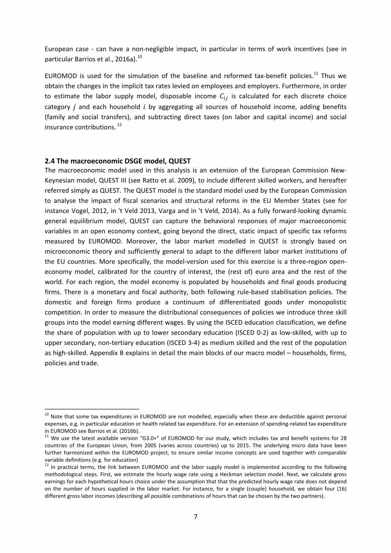
European  case  ‐  can have a non‐negligible  impact,  in particular  in  terms of work  incentives  (see  in 

particular Barrios et al., 2016a).10  

EUROMOD  is  used  for  the  simulation  of  the  baseline  and  reformed  tax‐benefit  policies.11  Thus we 

obtain the changes in the implicit tax rates levied on employees and employers. Furthermore, in order 

to  estimate  the  labor  supply model,  disposable  income    is  calculated  for  each  discrete  choice 

category    and  each  household    by  aggregating  all  sources  of  household  income,  adding  benefits 

(family  and  social  transfers),  and  subtracting  direct  taxes  (on  labor  and  capital  income)  and  social 

insurance contributions. 12  

 

2.4 The macroeconomic DSGE model, QUEST The macroeconomic model used  in  this analysis  is an extension of  the European Commission New‐

Keynesian model, QUEST III (see Ratto et al. 2009), to include different skilled workers, and hereafter 

referred simply as QUEST. The QUEST model is the standard model used by the European Commission 

to  analyse  the  impact  of  fiscal  scenarios  and  structural  reforms  in  the  EU Member  States  (see  for 

instance Vogel, 2012,  in  't Veld 2013, Varga and  in  't Veld, 2014). As a fully forward‐looking dynamic 

general  equilibrium model, QUEST  can  capture  the  behavioral  responses  of major macroeconomic 

variables  in an open economy context, going beyond the direct, static  impact of specific tax reforms 

measured  by  EUROMOD.  Moreover,  the  labor  market  modelled  in  QUEST  is  strongly  based  on 

microeconomic  theory and sufficiently general  to adapt  to  the different  labor market  institutions of 

the EU countries. More specifically,  the model‐version used  for  this exercise  is a  three‐region open‐

economy model,  calibrated  for  the  country of  interest,  the  (rest of)  euro  area  and  the  rest of  the 

world. For each  region,  the model economy  is populated by households and  final goods producing 

firms. There  is a monetary and  fiscal authority, both  following  rule‐based  stabilisation policies. The 

domestic  and  foreign  firms  produce  a  continuum  of  differentiated  goods  under  monopolistic 

competition. In order to measure the distributional consequences of policies we  introduce three skill 

groups into the model earning different wages. By using the ISCED education classification, we define 

the share of population with up to  lower secondary education  (ISCED 0‐2) as  low‐skilled, with up to 

upper secondary, non‐tertiary education (ISCED 3‐4) as medium skilled and the rest of the population 

as high‐skilled. Appendix B explains in detail the main blocks of our macro model – households, firms, 

policies and trade. 

 

                                                            10 Note that some tax expenditures  in EUROMOD are not modelled, especially when these are deductible against personal expenses, e.g. in particular education or health related tax expenditure. For an extension of spending‐related tax expenditure in EUROMOD see Barrios et al. (2016b). 11 We use  the  latest available version “G3.0+” of EUROMOD  for our study, which  includes  tax and benefit systems  for 28 countries of  the  European Union,  from  2005  (varies  across  countries) up  to  2015.  The underlying micro data  have been further harmonized within  the EUROMOD project,  to ensure  similar  income  concepts are used  together with  comparable variable definitions (e.g. for education) 12  In practical  terms,  the  link between EUROMOD and  the  labor  supply model  is  implemented according  to  the  following methodological steps. First, we estimate  the hourly wage  rate using a Heckman selection model. Next, we calculate gross earnings for each hypothetical hours choice under the assumption that that the predicted hourly wage rate does not depend on  the number of hours  supplied  in  the  labor market.  For  instance,  for a  single  (couple) household, we obtain  four  (16) different gross labor incomes (describing all possible combinations of hours that can be chosen by the two partners). 

 

8  

2.5. Aggregation issues The  interaction between  the micro and macroeconomic models described above  raises  consistency 

issues related with the way agents’ heterogeneity  is handled  in each of the frameworks. On the one 

hand,  the  discrete  choice model  allows  us  to  obtain  estimates  of  labor  supply  responses  at  the 

household micro data  level. On  the other hand,  the QUEST model provides  the general equilibrium 

effects  focusing  on  representative  households,  workers  and  firms,  and  the  impact  on  overall 

macroeconomic outcomes. This means  that we need  to combine different degrees of heterogeneity 

and  methods  of  handling  this  heterogeneity  among  models.  We  will  focus  the  discussion  on 

aggregation on the choice of selected structural parameters of QUEST and the role of the labor market 

in shaping the interaction between the microsimulation model and the macro‐DSGE model. 

Aggregation  is  a  controversial  topic when using dynamic  stochastic  general  equilibrium models  for 

policy predictions. Chang et al. (2013) find biases in policy predictions due to the lack of invariance in 

the structural parameters  in representative agent models. An  important strand of  the  literature has 

been  investigating  the  structural  nature  of  the  preferences  and  technology  parameters  of  DSGE 

models under different policy regimes,  including Altissimi, Siviero and Terlizzesse (2002), Fernández‐

Villaverde and Rubio‐Ramirez (2008), Cogley and Yagihashi (2010), to cite just a few. This question has 

direct  implications  for  the methods  chosen  to  take DSGE models  to  the data,  i.e.  to quantitatively 

evaluate  these models.  In  this paper, we  calibrate QUEST by  selecting behavioral and  technological 

parameters  so  that  the  model  replicates  important  empirical  ratios  such  as  labor  productivity, 

investment,  consumption  to  GDP  ratios,  the  wage  share,  the  employment  rate,  given  a  set  of 

structural  indicators  describing market  frictions  in  goods  and  labor markets,  tax wedges  and  skill 

endowments.13 Most of the variables and parameters are taken from available statistical or empirical 

sources  from  the  literature.  The  remaining  parameters  are  pinned  down  by  the  mathematical 

relationships of the model equations and by the steady‐state conditions. Regarding the labor market, 

we calibrate QUEST using the micro‐econometric information supplied by EUROMOD extended by the 

labor supply discrete choice model,  in order  to ensure consistency between  the  two models.  In  this 

way, we use the estimates for  labor supply elasticities, by skill  level, to calibrate the parameter   of 

the household utility function for the different skill groups considered (see Appendix B and C). In doing 

so, we assume that these elasticities are structural parameters which are tied to the utility  function 

and remain unchanged under a policy reform scenario. This means that we implement the tax reform 

in QUEST  by matching  the  tax  rates  on  labor  paid  by  employees  ( )  and  employers  ( ,)  to  the 

implicit  tax  rates obtained  from our microsimulation model. Note  finally  that  in QUEST households 

only decide on  the amount of hours supplied  in  the  labor market, but  they do not choose between 

unemployment  and  non‐participation,  explicitly.  The  non‐participation  rate  is  calibrated  as  the 

proportion  of  inactive  agents  in  the  total  population.  The  non‐participation  rate  (NPART)  must 

therefore be seen as an exogenous policy variable characterising the generosity of the benefit system. 

However,  in  our  discrete  choice  model  the  choice  of  non‐participation,  or  being  unemployed 

voluntarily,  is one of the possible alternatives of  individual  i. The choice of participating  in the  labor 

market  is nested  together with  the decision on  supplying different number of hours  (which  can be 

seen as the different working modalities). We reconcile the two models on this issue by calibrating in 

QUEST the non‐participation rate according to the expected number of  individuals that choose to be 

out of the labor market. Technical derivations of the labor supply function and respective elasticities in 

                                                            13 Supplementary data associated with the calibration of the QUEST III model can be found in the online version of Ratto et al. (2009) at http://publications.jrc.ec.europa.eu/repository/handle/JRC46465. 

 

9  

both  the micro and macroeconomic  settings are presented  in Appendix C where we also present a 

detailed description on the tax incidence assumptions in QUEST. 

3. Illustration: hypothetical social insurance contributions cuts in Belgium   To  illustrate the usefulness of our methodology, we analyse tax reforms  in three EU Member States: 

Belgium, Italy and Poland. In all three countries, the selected reforms aim at reducing the tax burden 

on  labor. While  in the Belgium case both employees and employers benefit from the tax reductions, 

the reform proposals for Italy and Poland only affect the labor supply side. In this section, we focus on 

a  hypothetical  reform  in  Belgium  which  would  reduce  the  social  insurance  contributions  paid  by 

employees and employers. More precisely, we simulate:  

i. a  reduction  of  the  social  insurance  contributions  rate  paid  by  employees  from  13.07%  to 

9.07% (by cutting 3 pp from pensions and 1 pp from health contributions); 

ii. a  reduction  of  the  standard  social  insurance  contributions14  rate  paid  by  employers  from 

25.36% to 17.75% (by cutting 5 pp from pensions and 2.6 pp from health contributions). 

In both scenarios, the total statutory tax rate of the social insurance contributions paid by employees 

and employers is cut by 30%, and we have translated this tax cut on the same specific contributions – 

pensions  and  health  contributions  –  so  that  the  reforms  "mirror"  each  other  and  their  fiscal  and 

distribution impact can be directly compared. 

   

3.1. First step: Labor market characterization and policy shocks  We  first  estimate  the  labor  supply  elasticities,  the  expected  voluntary  unemployment  rate  (non‐

participation rate) and calculate the change in implicit tax rates (the policy shocks) which will be used 

to calibrate QUEST.15   

Labor supply elasticities and non‐participaticipation rates Labor  supply  elasticities  are  estimated  using  the  discrete  choice  labor  supply model  described  in 

section 2.2. They are used  to calibrate  the parameter  ,  that determines  the Frisch elasticity  in  the 

DSGE model QUEST,  as  explained  in  detail  in  Appendix  C  (equations  C.23  to  C.41).  The  expected 

number  of  voluntary  unemployed  is  also  obtained  from  the  discrete  choice model  based  on  the 

estimated  probability  of  choosing  to  supply  zero  hours  in  the  labor market  (see  equation  (C.22) 

derived  in Appendix C). The elasticities, the corresponding value for parameter   as well as the non‐

participation  rate – calculated  for  three  skill categories,  respectively – are  shown  in Table 1.  In  line 

                                                            14 These standard social  insurance contributions  include contributions for pensions, healthcare, disabilities, unemployment, family allowances, accidents at work (standard and special), work‐related  illness (standard and asbestos fund), educational leave,  integration  and  guidance  programs  for  youth,  daycare  provision  and  (re)employment  of  vulnerable  groups.  The referred contributions have been substituted by the "global social insurance contribution", as for 2016. 15 In order to obtain the elasticities and the expected voluntary unemployment rate, we use version G3.0 of the EUROMOD microsimulation model,  together with  the datasets based on  the 2012 version of EU‐SILC. This  is  the most  recent dataset available that can be  linked with tax‐benefit rules for the  income reference period which  is necessary for the estimation of the labor supply model. For the simulation of the tax reforms, we choose 2013 tax‐benefit rules as the baseline. This is the most recent policy year that can be simulated with EUROMOD at the time of writing this paper. Uprating factors are used to update the non‐simulated income components to 2013. 

 

10  

with the literature, we find that labor‐supply elasticities as well as non‐participation rates are highest 

for the low‐skilled (see e.g. Bargain et al. 2014). 

Table 1. Calibration of labor supply elasticity parameter and nonparticipation rates, by skill level, in 

QUEST 

Labor supply elasticities  Parameter  Non participation rates 

High  Medium Low  High Medium Low High Medium  Low 

0.357  0.395 0.716  0.351 0.631 0.978 0.057 0.107  0.246 

 

Policy shocks The reform of the Belgium tax and benefit system is implemented in EUROMOD by changing the social 

insurance  contribution  rates  levied  on  employees  and  employers. We  employ  the  implicit  tax  rate 

formula used by the European Commission (2013) in order to derive the implied change in employees’ 

and  employers’  tax  burden  in  the  baseline  and  reform  scenarios  for  low, medium  and  high‐skilled 

workers, respectively: 

∑ ∗

, ∈ , ,                                                                                               

 is the ratio of wages relative to the total taxable income of taxpayer i: 

 

  is  the  personal  income  tax  liability  of  individual  i,      and  are  the  social  insurance contributions paid by employees and employers, respectively. From the   expression, we can derive 

the implicit tax rates for employees ( , ) and employers ( , ): 

,∑ . ∗

, ∈ , ,      

and 

, , ∈ , ,                                                                                                

In QUEST, the corresponding tax policy variables are the statutory tax rates on labor and firms,    and 

, respectively. They are defined in terms of gross wages, that is, the tax burden levied on employees 

and firms is given by  ∗  and  ∗ , respectively.16 Statutory and implicit 

tax rates are related as follows: 

, ∗ ∗ , ∗  

and 

, ∗ , ∗  

                                                            16 See Appendix C for a description of the tax incidence analysis in QUEST. 

 

11  

It follows that: 

,,

1 , 

and 

,,

1 , 

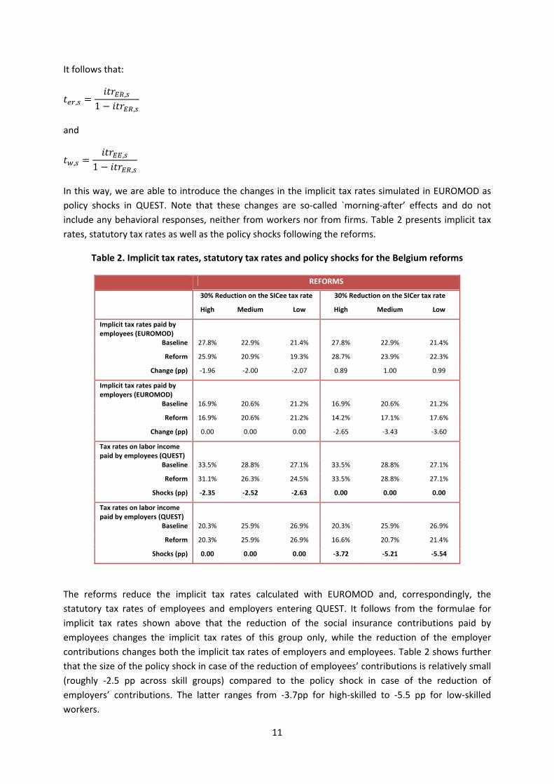
In this way, we are able to  introduce the changes  in the  implicit tax rates simulated  in EUROMOD as 

policy  shocks  in QUEST. Note  that  these  changes  are  so‐called  `morning‐after’  effects  and  do  not 

include any behavioral responses, neither from workers nor from firms. Table 2 presents  implicit tax 

rates, statutory tax rates as well as the policy shocks following the reforms.   

Table 2. Implicit tax rates, statutory tax rates and policy shocks for the Belgium reforms 

  REFORMS 

  30% Reduction on the SICee tax rate 30% Reduction on the SICer tax rate 

  High  Medium Low High Medium  Low 

Implicit tax rates paid by employees (EUROMOD) 

     

Baseline  27.8%  22.9% 21.4% 27.8% 22.9%  21.4% 

Reform  25.9%  20.9% 19.3% 28.7% 23.9%  22.3% 

Change (pp)  ‐1.96  ‐2.00 ‐2.07 0.89 1.00  0.99 

Implicit tax rates paid by employers (EUROMOD) 

   

Baseline  16.9%  20.6% 21.2% 16.9% 20.6%  21.2% 

Reform  16.9%  20.6% 21.2% 14.2% 17.1%  17.6% 

Change (pp)  0.00  0.00 0.00 ‐2.65 ‐3.43  ‐3.60 

Tax rates on labor income paid by employees (QUEST) 

   

Baseline  33.5%  28.8% 27.1% 33.5% 28.8%  27.1% 

Reform  31.1%  26.3% 24.5% 33.5% 28.8%  27.1% 

Shocks (pp)  ‐2.35  ‐2.52 ‐2.63 0.00 0.00  0.00 

Tax rates on labor income paid by employers (QUEST) 

   

Baseline  20.3%  25.9% 26.9% 20.3% 25.9%  26.9% 

Reform  20.3%  25.9% 26.9% 16.6% 20.7%  21.4% 

Shocks (pp)  0.00  0.00 0.00 ‐3.72 ‐5.21  ‐5.54 

 

The  reforms  reduce  the  implicit  tax  rates  calculated  with  EUROMOD  and,  correspondingly,  the 

statutory  tax  rates  of  employees  and  employers  entering QUEST.  It  follows  from  the  formulae  for 

implicit  tax  rates  shown  above  that  the  reduction  of  the  social  insurance  contributions  paid  by 

employees  changes  the  implicit  tax  rates  of  this  group  only, while  the  reduction  of  the  employer 

contributions changes both the implicit tax rates of employers and employees. Table 2 shows further 

that the size of the policy shock in case of the reduction of employees’ contributions is relatively small 

(roughly  ‐2.5  pp  across  skill  groups)  compared  to  the  policy  shock  in  case  of  the  reduction  of 

employers’  contributions.  The  latter  ranges  from  ‐3.7pp  for  high‐skilled  to  ‐5.5  pp  for  low‐skilled 

workers.  

 

12  

Labor supply effects from the augmented microsimulation model We  report  labor  supply  responses  to  the  employees  social  insurance  reform  in  terms of  aggregate 

weekly full time equivalent jobs in Table 3,17 separately for the intensive and extensive margin.18 The 

predictions for the baseline and the employees social insurance contribution reform are based on the 

estimated labor supply model described in section 2.2.19 

Table 3: Employment effects from the Belgian employees reform 

Changes in full time equivalents

    total  intensive  extensive 

30% Reduction on the SICee tax rate 

baseline  2,920,764  2,735,788  184,976 

reform 2,957,053 2,768,090  188,963

% change  1.242 1.181  2.156

 

We find particular  large effects on the extensive margin. This  is  in  line with the  literature,20 and also 

confirmed by our findings of larger extensive than intensive margin elasticities.  

Recall  that we  consider a decrease  in  social  insurance  contributions on both  the employer and  the 

employee  side.  As we  start  our  analysis with  the microsimulation model,  the  labor  supply  effects 

reported  in  Table  3  for  Belgium  are  the  effects  from  the  decrease  in  employee  SIC  only,  as  the 

decrease on employer SIC does not affect household disposable  incomes at  this stage.21 The reform 

leads to an increase in aggregate labor supply of 1.24%. 

 

3.2. Second step: The macroeconomic impact 

We calibrate QUEST for Belgium, the rest of the euro area and the rest of the world.22 As explained in 

the previous section, we calibrate the parameter   and the non‐participation rate, NPART, based on 

the elasticities and predicted  labor  supply  responses obtained  from  the discrete  choice model. The 

changes  in  the  implicit  tax  rates  on  labor  paid  by  employees  and  employers  are  introduced  as 

permanent policy shocks in QUEST. For that we have also set off the debt‐stabilization rule (equation 

(B.21)  in  Appendix  B)  for  the  first  fifteen  years,  otherwise  the  tax  rate  on  labor  income  paid  by 

employees would automatically change after the shock in order to close the deficit generated by the 

tax cut, as expressed in equation (B.21) in Appendix B. 

                                                            17 We calculate full time equivalents by dividing aggregate expected weekly working hours by 40. 18 The intensive margin is the hours effect on those observed to be working, while the extensive effect is the change in hours for  those observed  to be not working  (see Bargain et al. 2014). The  total effect  is  the average of  intensive and extensive margin effects, weighted by their respective share of the population. 19 We  only  report  results  on  aggregate  hours. Detailed  regression  results  of  the  discrete  choice model  are  available  on request. 20 See Chetty (2012) and Chetty et al (2012). 21 In principle, second‐round effects can occur if the decrease in employer SIC is not fully born by employers, but passed on to the workers. In our modelling framework, second‐round effects are considered in QUEST. 22  For  a  complete  description  of  the  full  calibration  of  QUEST  see  the  online  version  of  Ratto  et  al.  (2009)  at http://publications.jrc.ec.europa.eu/repository/handle/JRC46465. In this paper, we focus only on the calibration of selected parameters related directly to the labor market. 

 

13  

Impulse responses and tax incidence  

The introduction of the shocks for each of the reforms in QUEST originates impulse responses for the 

model's endogenous variables. Selected  impulse response functions for the  labor market variables – 

net real wages,23 total compensation of employees,24 gross real wages, and employment – generated 

by  the  fiscal  shocks  produced  by  each  of  the  reforms  implemented  above  can  be  found  in  the 

Appendix D (graphs D.1 to D.8).  

Graphs D.1 to D.4 show the impulse response functions of the reform on employees contributions. We 

observe that net real wages of all skill groups jump immediately after the tax cuts are introduced and 

remain relatively stable afterwards. The total compensation of employees falls for all skill groups but 

in  a  smoother way,  since,  for  this  reform,  the  tax  burden  of  employers  remains  constant  in  our 

simulations and the changes derive only from the smooth decrease in gross wages, as we can observe 

from graph D.3. Employment increases over the simulation period. 

Graphs  D.5  to  D.8  show  the  impulse  response  functions  related  with  the  reform  on  employers 

contributions. In this case, the total compensation of employees immediately drops for all skill groups 

after the tax cut is introduced. It then begins to smoothly recover along the period of analysis due to 

the  increase  in gross wages  (see graph D.7) which  is also driving  the evolution of net  real wages  ( 

graph D.5). Employment increases over the simulation period as in the previous reform. 

Although the general equilibrium effects influence the numerical results – since output, consumption, 

capital utilisation and prices are  fully endogenous  in  the model –  the partial equilibrium analysis of 

Figures 2 and 3 can  illustrate the basic wage setting mechanism  in the QUEST model and explain the 

impulse response functions just described. These figures also illustrate the role played by tax incidence 

after the different policy shock are  introduced  in QUEST.  In Figures 2 and 3,    is the  labor demand 

function  (corresponding  to  equation  (B.15)  in  Appendix  B),  and    is  the  labor  supply  function 

(equivalent of equation  (B.7)  in Appendix B).  For  simplicity, we  assume  that  all other  variables  are 

constant, except real gross wages and  labor, and there are no adjustment costs. Let us also assume 

that in this partial equilibrium setting movements of the labor supply and labor demand functions are 

only due to the changes in the labor tax rates,   and , i.e. due to the policy shocks. 

Figure  2.  QUEST  partial‐equilibrium  effects  of 

the  reduction of  social  insurance  contributions 

paid by employees 

Figure  3.  QUEST  partial‐equilibrium  effects  of 

the  reduction of  social  insurance  contributions 

paid by employers 

                                                            23 Net real wages are defined as gross wages minus taxes paid by employees, as in expression (C.42) in Appendix C. 24 Total compensation of employees is defined as the sum of gross wages with the taxes paid employers on labor income, as in expression (C.43) in Appendix C. 

 

14  

 

From Figure 2, we observe that when   decreases workers are willing to offer more labor services for 

all  levels of  the  gross wage,  and   moves down  and  to  the  right  (i.e.  from    to  ).  In  the new 

equilibrium  , gross wages are lower and firms will be willing to hire more labor. This result is indeed 

confirmed by our impulse response functions for wages and employment (graphs D.3 and D.4). These 

results are also consistent with the partial equilibrium analysis of tax  incidence described analytically 

in Appendix C. In particular, the responses of net wages and of the total compensation of employees 

to an increase in labor tax are negative and positive, respectively, and are constrained by the elasticity 

of  labor supply ( , 0) and  labor demand ( , 0). Our shocks  imply that    0 and  0, 

then  from equation  (C.49) gross wages  should go down,  i.e.  <0.  In  the  same way, and now  from 

equation  (C.51), we  should  expect  the  net wages  to  rise  in  the  new  equilibrium. Note  that 

0, and, according  to equation  (C.51),  there  is an  inverse  relationship between  the change  in 

total taxes on labor income and net wages. This is also confirmed by the impulse response functions of 

the net wages (graph D.1). Finally, in what concerns the total compensation of employees paid by the 

firms, and according  to equation  (C.53), we  should expect  it  to decrease. Equation  (C.53)  implies a 

positive relationship between the change in total taxes on labor income and the total compensation. 

In  our  case,  0.  So,  the  total  compensation  of  employees  will  decrease  in  the  new 

equilibrium.  Again  this  is  shown  in  the  impulse  response  functions  of  the  total  compensation  of 

employees, in graph D.2. 

A similar analysis can be done from Figure 3. When   decreases firms are willing to hire more labor 

services for all levels of the gross wage, and   moves up and to the right (i.e. from   to  ). In the 

new equilibrium  , gross wages are  lower and firms are willing to hire more  labor at the new wage 

rate. This  result  is  indeed confirmed by  the  impulse  response  functions  for wages and employment 

(graphs D.3 and D.4). Again drawing from our tax  incidence analysis and since our shocks  imply that  

0 and  0, from equation (C.49) gross wages should go up, i.e.  <0. In the same way, and 

now  from  equation  (C.51), we  should  expect  the  net wages  to  rise  in  the  new  equilibrium, 

0, and, according  to equation  (C.51),  there  is an  inverse  relationship between  the change  in total taxes on labor income and net wages. This is also confirmed by the impulse response functions of 

the net wages (graph D.5). Finally, in what concerns the total compensation of employees paid by the 

firms, and according  to equation  (C.53), we  should expect  it  to decrease. Since  0,  the total  compensation  of  employees will  decrease  in  the  new  equilibrium. Again  this  is  shown  in  the 

impulse response functions of the total compensation of employees, in graph D.6. 

 

15  

Sensitivity analysis We have also performed a sensitivity analysis  in order to understand how dependent our results are 

on  the  type of shocks considered and on selected QUEST parameters and variables.  In  this way, we 

have  considered  the  following  three  alternative  scenarios  as  a  comparison with  the  reform on  the 

employers contributions: 

i. Scenario  1:  To  replicate  the  policy  shocks  of  the  employers  contributions  reform  on  the 

employees  contributions  leaving unchanged  the baseline  social  insurance contributions  rate 

paid  by  employers.  This means  that  ex‐ante, without  any  behavioral  effect  one would  get 

exactly  the  same  cut  in  labor  tax  revenues  from  this  reform  and  the  previous  reform  on 

employers contribution. 

ii. Scenario  2:  To  consider  a  new  baseline  with  half  of  the  Frisch  elasticities  of  the  original 

estimates,  for  each  skill  group,  and  apply  the  policy  shocks  derived  from  the  employers 

contributions reform 

iii. Scenario 3: To consider a new baseline with half of  the nominal wage and price adjustment 

costs and apply the policy shocks derived from the employers contributions reform. 

Figures 4  to 6 below  show  the  impulse  responses  for  selected variables –  labor  tax  revenues,  total 

gross wages and total employment – obtained for each of the three scenarios described above and for 

the  reform on employers  contributions. Besides  these  four  scenarios,  Figure 4  also plots  the  static 

revenue  estimate  scenario,  which  reflects  only  the  mechanical  tax  cut  on  the  employers  social 

insurance contributions without the endogenous wage and employment response (denoted by "SICer 

reform no behavior").  

Figure 4. Labor tax revenues impulse responses (quarterly pp deviations from baseline) 

  

Figure 5. Total gross wages impulse responses (quarterly pp deviations from baseline) 

Figure 6. Total employment impulse responses (quarterly pp deviations from baseline) 

 

‐9

‐8

‐7

‐6

‐5

‐4

1 2 3 4 5 6 7 8 9 10 11 12

SICer reform (no behaviour)

SICer reform

Scenario 1

Scenario 2

Scenario 3

 

16  

   

From Figure 4, we observe  that  labor  tax  revenues decrease upon  the policy shock  for all  the cases 

considered, as expected. However, we observe that when the tax cut  is  implemented by cutting the 

employers social insurance contributions, the decrease in these revenues gets smaller over the period 

of analysis, revealing that this reform is to some extent self‐financing. This self‐financing effect can be 

explained by the trajectories of wages and employment: from Figures 5 and 6, we observe that when 

the  tax cut affects  firms, both  the wage and employment have  increasing  trajectories. This  result  is 

robust with respect  to the  labor supply elasticity, the wage and price adjustment costs: the  impulse 

responses  obtained  for  scenarios  2  (lower  Frisch  elasticity)  and  3  (lower  nominal wage  and  price 

adjustment  costs)  follow  closely  the  ones  for  the  employers  social  insurance  contribution  reform. 

From Figure 4, we also observe that in scenario 1 – where exactly the same tax cuts assigned before to 

employers are now granted to employees –  labor  tax revenues decrease steadily over the period of 

analysis. This result can be explained by the wage and employment trajectories shown in Figures 5 and 

6: when the tax cut affects employees only, the wage and employment effects cancel each other. As a 

consequence, we obtain only very modest self‐financing effects which are close to the "no‐behavior" 

situation. This result is in line with the trajectories obtained for wages and employment for employee 

social insurance contributions reform (see Table 4 below). 

Feedback effects Following  the  standard  practice  in  dynamic  scoring  exercises, we  can  also  quantify  the  behavioral 

feedback effects of the reforms. Table 3 shows the revenue feedback effect for each scenario which is 

defined as  the percentage difference of  the  revenue effect produced by  the macroeconomic model 

relative to the static revenue estimate (see JCT, 2005). This measure allows us to quantify the extent 

to which  the  reforms are  self‐financing  through economic growth  (in our context changes  in wages 

and employment). We also decompose  the  revenue  feedback effect  into  the endogenous  feedback 

contribution from wages and employment respectively. 

Table 3. Decomposing the revenue feedback effects of tax reform scenarios (% changes relative to 

static estimates) 

Years  3 ys  5 ys 

Employee tax‐cut, BE  6.4  12.9 

‐2

‐1

0

1

2

3

4

5

1 2 3 4 5 6 7 8 9 10 11 12

SICer reform

Scenario 1

Scenario 2

Scenario 3

‐2

‐1

0

1

2

3

4

5

1 2 3 4 5 6 7 8 9 10 11 12

SICer reform

Scenario 1

Scenario 2

Scenario 3

 

17  

 ‐ effect from employment  18.3  23.0 

 ‐ effect from wages  ‐11.9  ‐10.1 

Employer tax‐cut, BE  48.7  50.3 

 ‐ effect from employment  13.2  12.5 

 ‐ effect from wages  35.4  37.8 

Note: Positive percentage change indicates that the estimated revenue loss is less when the macroeconomic effects are taken into account 

while negative percentage change indicates higher revenue loss compared to the static estimate.    

The  reform  implemented  on  the workers'  side  generates  lower  feedback  effects  compared  to  the 

reduction of firms' tax burden. By the end of the three year period, the combined effect of wages and 

employment accounts for self‐financing of about 6.4% of the reduction  in total  labor tax revenues  in 

case of the reform of employees' social insurance contributions. The self‐financing effect amounts to 

almost 50%  in case of  the employers' social  insurance contribution  reform. The magnitude of  these 

feedback effects is close to the dynamic scoring results of Mankiw and Weinzierl (2006). These authors 

find  that  in  a  standard  neoclassical model,  up  to  half  of  a  capital  tax  cut  can  be  self‐financing. 

However, they obtain substantially lower feedback effect from a labor tax cut, ranging from 0% to 17% 

depending on  the  labor  supply  elasticity.25 Other dynamic  scoring  studies  including  JCT  (2005)  and 

Trabandt  and  Uhlig  (2011)  report  similar  patterns  for  labor  and  capital  tax  reform  scenarios. Our 

model‐simulations confirm the same pattern with respect to cuts in employee vs. employer paid taxes 

on  labor. In  line with the theoretical predictions (see Figure 2‐3), Table 3  illustrates that this result  is 

due  to  the different behavioral effects of wages under  the  two  scenarios: decreasing  the  firms'  tax 

burden  induces  an  upward  pressure  on wages,  increases  the  tax‐base  and  the  corresponding  self‐

financing rate is up to 37½ % after five years. On the other hand, cutting the tax burden on employees 

has  the  opposite  effect  on  the  tax‐base  due  to  the  downward  pressure  on  wages  and  the 

corresponding  self‐financing  rate  is  down  by  around  10  pp.. Notice,  that  the  feedback  effect  from 

employment  is  positive  in  both  cases:  higher  employment  increases  the  tax‐base  and  the 

corresponding self‐financing rates are up by around 23 pp. (employee tax‐cut) and 13 pp. (employer 

tax‐cut) respectively after five years. 

Macroeconomic trajectories The  final  annualized macroeconomic  impact  on  the  variables  of  interest  from  the  tax  reforms  is 

summarized in Table 4 below. 

Table 4. Macro impact of the tax reforms (annualized % deviation from baseline) on the variables of 

interest, based on QUEST simulations 

  REFORMS

  30% Reduction on the SICee tax rate 30% Reduction on the SICer tax rate 

  T+1  T+2 T+3 T+1 T+2 T+3 

Price level  ‐0.043  ‐0.101 ‐0.128 ‐0.096 ‐0.161 ‐0.154 

Employment      

Low skilled  0.171  0.444 0.739 0.825 1.338 1.445 

Medium skilled  0.233  0.556 0.847 0.790 1.292 1.443 

High skilled  0.278  0.614 0.874 0.449 0.720 0.868 

                                                            25  In general, they find that,  independently on how  labor supply  is calibrated, "if capital and  labor tax rates start off at the same level, cuts in capital taxes have greater feedback effects in the steady state then cuts in labor taxes".  

 

18  

Gross real wage      

Low skilled  ‐0.225  ‐0.437 ‐0.527 1.379 2.867 3.576 

Medium skilled  ‐0.334  ‐0.566 ‐0.619 1.336 2.749 3.370 

High skilled  ‐0.397  ‐0.628 ‐0.627 1.143 2.282 2.732 

 

As  already mentioned,  the main  difference  between  the  two  reforms  consists  in  the  sign  of  the 

trajectories for wages: while the cut  in the social  insurance contributions paid by workers generates 

downward  trajectories  for wages  for  all  skill‐groups,  the  reduction  in  the  employers'  contributions 

generates upward ones. This implies counteracting behavioral effects in the context of the employees 

reform,  resulting  in  small but non‐negligible differences between  the  "no behavior" and  "behavior" 

scenarios considered in the last step of our analysis, as we will confirm in the next section. 

 

3.3. Third step: Microsimulation results In  the  third  step of our dynamic  scoring exercise, we  input  the  impulse  responses  for employment, 

gross  real  wages  and  consumer  price  index  generated  by  the  QUEST  model  back  into  the 

microsimulation model in order to assess the medium‐term projections in tax revenues, contributions, 

benefits  and  disposable  incomes.  In  addition, we  simulate  a  second  scenario  in which  the  second 

round  effects,  i.e.  the macroeconomic  feedback  and  behavioral  response  to  the  tax  change,  are 

disregarded.   

We analyse both scenarios over the period   to  and compare the variation in tax revenues, social 

insurance contributions, and disposable income against the baseline. More precisely, we apply the tax 

system  of  the  baseline  policy  year    to  the  subsequent  three  years,  accommodating  only  the 

adjustments in the monetary variables by using the standard uprating factors. As explained previously, 

in EUROMOD, the uprating factors are utilized as discount factors to update monetary variables to the 

price level of the year for which the tax system is analysed. This update is necessary because the input 

data files to EUROMOD always come with a  lag, given that they are survey data. The  input data files 

used here  are based on EU‐SILC 2012  survey data, which do not  correspond with  the most  recent 

(simulated)  tax‐benefit  system  that  is modified with  the  simulated  reforms. Therefore,  the uprating 

factors allow for time consistency between the monetary variables of the survey and the tax system 

under analysis.26 We assess  the  fiscal and equity  impact of  the  tax  reforms embedding  the  second‐

round  effects  by  amending  the  uprating  factors  and  the  weights  in  the  household  micro‐data  

according  to  the  macroeconomic  feedback  provided  by  the  QUEST  model  (Table  4)  for  prices, 

employment and wages. This is done as follows: 

a) We  incorporate  the macro  impact of  the  tax  reforms on employment by adapting  the  input 

dataset to accommodate the QUEST trajectories for the medium‐term. In order to do so, we 

create micro‐datasets for each year of analysis ( ,  ,  ).  For each skill group, the weights of 

the  employed  are  increased  according  to  the  corresponding  impulse  response,  while  the 

                                                            26 The only shortfall of this approach concerns the missing uprating factors for the policy year 2016 (as the  latest available version of EUROMOD at the time of the analysis ran on the 2015 tax and social benefit system).  In order to overcome this limitation,  for  each  monetary  variable  we  estimate  the  2016  uprating  factors  by  taking  into  account  the  European Commission  forecast of proxy variables  (or  the  same variable, when available). The macroeconomic  forecasts are publicly available in the AMECO database (http://ec.europa.eu/economy_finance/db_indicators/ameco/index_en.htm). 

 

19  

weights of  the unemployed  are  scaled down  keeping  the  total population  constant.  In  this 

way, the employment effect estimated in QUEST is fully implemented as an extensive margin 

effect in the household micro‐data. 

b) The impulse response for the consumer price index is integrated in EUROMOD as a correction 

of the correspondent uprating factor. 

c) For gross wages we apply the same approach as for the CPI, with the only exception of having 

uprating factors for each skill category.  

We subsequently run the microsimulation model to quantify the overall budgetary and distributional 

effects of the reforms under the two scenarios.  

The microsimulation results are presented in detail in Figures 7‐12. Figures 7 and 8 present the impact 

on  the  two  affected  subcomponents  of  employee  and  employer  social  insurance  contributions  – 

pension  and  health  insurance  contributions  – while  Figures  9  to  12  show  the  impact  on  broader 

categories of tax revenues (i.e. government revenue from personal income taxes and social insurance 

contributions) as well as the impact on household disposable income by income decile.  

Figure 7. Employee contribution impact in EUROMOD incorporating macro feedback on prices, 

wages and employment – Belgium 

 

 

Figure 8. Employer contribution impact in EUROMOD incorporating macro feedback on prices, 

wages and employment – Belgium 

 

‐40,3%

‐40,1%

‐39,9%

‐39,7%

‐39,5%

2013 2014 2015 2016

Employee contribution to pension insurance

Tax policy change, nobehavioural reaction

Tax policy change, includingbehavioural reaction

‐28,3%

‐28,2%

‐28,1%

‐28,0%

2013 2014 2015 2016

Employee contribution to health insurance

‐57%

‐56%

‐55%

‐54%

‐53%

2013 2014 2015 2016

Employer contribution to pension insurance

Tax policy change, nobehavioural reaction

Tax policy change, includingbehavioural reaction

‐40%

‐39%

‐38%

‐37%

‐36%

‐35%

2013 2014 2015 2016

Employer contribution to health insurance

 

20  

Figures 7 and 8 show that: 

When  the  reform  is  implemented on  the workers'  side,  the employee  social  insurance  contributions 

decrease both  in  the presence and  in  the absence of  second‐round effects.  In  t1 and  t2,  the drop  is 

larger  in  the  scenario  accounting  for  second‐round  effects  since  the  new  equilibrium  in  the  labor 

market  implies  lower gross wages, and consequently  lower social  insurance contributions. However, 

we  find  that  the positive employment effect counterbalances  the negative wage effect  leading  to a 

lower tax revenue loss in t3. The overall tax revenue loss is similar in both scenarios. Pension (health) 

insurance contributions decrease by around 40% (28%).  

When  the  reform  is  implemented  on  the  firms'  side,  the  employer  social  insurance  contributions 

decline at different rates, depending on the affected tax category. In the scenario ignoring behavioral 

responses,  the  loss  in health  insurance  contributions  amounts  to  almost 40%  in  year  t1.  It  is more 

significant for pension  insurance contributions (roughly 57%).  In the scenario accounting for second‐

round  effects,  the  revenue  loss  is  marginally  smaller  (by  almost  1  pp.  for  both  tax  categories). 

Furthermore, the gap between the behavioral and non‐behavioral scenario widens gradually from one 

year to another, reaching 2 pp. in year t3. This results from the expansion in labor demand that pushes 

up both wages and employment. 

Figures 9 and 10 below show the impact of the two tax reform on broader tax categories (total net tax 

revenues27, personal income taxes and social insurance contributions). 

Figure 9. Impact of the employee SIC reform on aggregate tax revenues – Belgium

 

  

                                                            27  By  total  net  tax  revenues  we  refer  to  the  government  revenues  derived  from  simulated  taxes  and  social  security contributions net of means‐tested and non means‐tested benefits (excluding pensions).     

‐6%

‐4%

‐2%

0%

2013 2014 2015 2016

Total net tax revenues

Baseline (no policy change)

Tax policy change, no behavioural reaction

Tax policy change, including behavioural reaction

0%

2%

4%

6%

8%

2013 2014 2015 2016

Personal Income Taxes

‐40%

‐30%

‐20%

‐10%

0%

2013 2014 2015 2016

SIC Employees

‐0,3%

‐0,2%

‐0,1%

0,0%

0,1%

2013 2014 2015 2016

SIC Employers

 

21  

Figure 10. Impact of the employer SIC reform on aggregate tax revenues – Belgium

 

 

From these figures, we observe that: 

i. When  the  reform  is  implemented  on  the  workers'  side,  the  reduction  in  social  insurance 

contributions paid by employees  leads  to a  fall  in  total net government  revenues of almost 

3.8% in t3. This drop is the result of two direct (morning‐after) effects that evolve in opposite 

directions: on the one hand, decreasing employees' social incurance contributions, and, on the 

other, increasing revenues from personal income taxation (as the taxable income, which is net 

of social contributions, broadens). The evolution of total net tax revenues differs slightly when 

we  consider  second‐round effects:  in  the  first  two years  following  the  reform,  total net  tax 

revenues are lower compared to the no‐behavior scenario, but are higher in year t3. The effect 

of decreasing gross wages pushing down total tax revenues dominates  in t1 and t2. However, 

starting  in year  t3  the positive employment effect outweights  the negative wage effect.28 As 

regards the social  insurance contributions paid by employers, we observe that they shrink  in 

the first year, but start to recover afterwards slightly exceeding the baseline level by the end 

of  the  analysed period.  This  can  again be  explained by  the  simultaneous decrease  in  gross 

wages  (and  correspondent decrease  in  contributions paid) and  the  increase  in employment 

with the latter effect being stronger at the end of the simulation period.  

ii. When the reform is implemented on the firms' side, the immediate revenue loss in t1 amounts 

to  9.8%  (non‐behavior  scenario).  Incorporating  the macro  feedback  on  prices,  wages  and 

employment we find that the revenue loss is smaller (7.2%) and shrinks to 3.9% by year t3, i.e. 

a reduction of roughly 60% (from 7.2 to 2.9 billion euros). This is due to the positive effect on 

                                                            28  The  positive  employment  effect  also  reduces  unemployment  benefit  expenditure  which  contributes  to  the  stronger increase in total net government revenues in the scenario including behavioral reactions. 

‐12%

‐10%

‐8%

‐6%

‐4%

‐2%

0%

2013 2014 2015 2016

Total net tax revenues

Baseline (no policy change)

Tax policy change, no behavioural reaction

Tax policy change, including behavioural reaction

0%

2%

4%

6%

2013 2014 2015 2016

Personal Income Taxes

0,0%

1,0%

2,0%

3,0%

4,0%

5,0%

2013 2014 2015 2016

SIC Employees

‐30%

‐25%

‐20%

‐15%

‐10%

‐5%

0%

2013 2014 2015 2016

SIC Employers

 

22  

both wages and employment, raising the revenues from personal  income taxes by 5.2%  in t3 

and  from  employees'  social  insurance  contribution  by  4.3%.  In  constrast  to  the  previous 

reform,  the  positive  employment  effect  is  now  amplified  by  a  positive  wage  effect.29  In 

addition, non‐means tested benefits decline by 2.3% due to the decrease in unemployment. 

In Figures 11 and 12 below we look at the impact of the simulated reforms on equivalised disposable 

income by income deciles. 

Figure 11.  Impact of  the employee SIC reform on disposable  income  (by  income decile) – Belgium

 

 

                                                            29 Wages growth is up to 3.5% for the low‐skilled in t3.  

 

23  

Figure 12. Impact of the employer SIC reform on disposable income (by income decile) – Belgium

 

From these figures, we observe that: 

i. When the reform is implemented on the workers' side, only the first decile is worse off at the 

end of  the simulation period  (scenario  including behavioral  reactions). This  is mainly due  to 

the small share of wage earners in this decile and due to the limited impact of the reform on 

their  social  insurance  contributions. Consequently,  the negative effect on wages offsets  the 

positive (morning‐after) effect on disposable income. The effect is regressive as lower deciles 

benefit  less  from  the  reform  than  the  top  of  the  distribution.  The  increase  in  disposable 

income for the bottom (top) three deciles is smaller (larger) than 1% (2%) by year t3.  

ii. When  the  reform  is  implemented on  the  firms' side,  the  reform  raises household disposable 

income only  in  the  scenario  including behavioral  responses, with  the  exception of  the  first 

decile. The cut in the employers' contributions has no no direct first‐order distributive effects. 

The  positive  effects  on  disposable  income  comes  through  the  labor  demand  expansion, 

increasing both wages and employment. This expansion has a regressive  impact with  largest 

gains for the top deciles. In spite of improving labor market conditions, the first decile faces a 

loss  in disposable  income which can be explained by a  reduced  receipt of benefit payments 

caused by the wage and employment increase.  

4. Extensions: Evaluating tax reforms in Italy and Poland We  use  the methodology  illustrated  in  the  previous  sections  to  evaluate  two  reforms:  an  already 

implemented refundable tax credit for workers in Italy and an announced, but not legislated increase 

in the universal tax credit in Poland. More specifically, the two reforms consist in: 

 

24  

i. The introduction, in May 2014, of a refundable in‐work tax credit for low income earners. This 

measure has been made permanent as of 201530, resulting in a tax credit of EUR 960 per year. 

The maximum amount (i.e. EUR 80 euro month) is given to employees with a taxable income 

below EUR 24.000 per year. Above this threshold, the tax credit is linearly decreasing up to a 

maximum taxable income of EUR 26.000. In order to be eligible for the bonus, the employees 

must earn at  least 8.000 euro per year (below the  limit, the employee does not pay  income 

tax). 

ii. An increase in the income exempt from the personal income tax from PLN 3,090 to PLN 8,000 

that was planned to be introduced by the recently appointed government on 1st January 2017 

(though  there  has  been  no  official  draft  legislation).  The  increase  in  the  tax‐free  amount 

implies that the amount of the universal tax credit rises from PLN 556 up to PLN 1,440, due to 

the fact that the tax base free of taxation is derived by dividing the universal tax credit31 to the 

tax rate of the first tax bracket (18%). 

A  priori,  both  reforms  increase  incentives  to  participate  in  the  labor market.32  The  labor  supply 

elasticities  and  the  non‐participation  rates  computed  in  order  to  calibrate QUEST  for  each  of  the 

countries of interest are shown in Table 5. 

Table 5. Calibration of labor supply elasticity parameter and nonparticipation rates, by skill level, in 

QUEST 

Countries  Labor supply elasticities  Parameter  Non participation rates 

  High  Medium  Low  High Medium Low High Medium  Low

Italy  0.199  0.201  0.301 0.896 1.497 2.485 0.079 0.132  0.290

Poland  0.311  0.271  0.598 0.515 1.776 1.173 0.102 0.214  0.270

 

The  changes  in  the  implicit  tax  rates obtained  from EUROMOD as well as  the correspondent policy 

shocks to be introduced in the QUEST model are presented in Table 6. 

Table 6. Implicit tax rates, statutory tax rates and policy shocks for the Italian and Polish reforms 

  REFORMS 

  Introduction in‐work tax credit in Italy Increase in universal tax credit in Poland 

  High  Medium Low High Medium  Low 

Implicit  tax  rates  paid  by employees (EUROMOD) 

     

Baseline  23.3%  19.7% 17.5% 16.7% 15.5%  15.8% 

Reform  22.1%  17.6% 14.9% 15.0% 13.5%  13.7% 

Change (pp)  ‐1.15  ‐2.12 ‐2.58 ‐1.66 ‐1.97  ‐2.07 

Implicit  tax  rates  paid  by employers (EUROMOD) 

     

Baseline  17.1%  17.2% 17.1% 17.1% 17.2%  17.1% 

Reform  17.1%  17.2% 17.1% 17.1% 17.2%  17.1% 

                                                            30 With the Stability Law for 2015 (n.190 of 2014). 31 The value of the universal tax credit in Poland is defined in The Natural Persons' Income Tax Act (PLN 556 per year). 32 Similarly to the Belgium reform, we use version G3.0 of the EUROMOD microsimultion model, together with the datasets based on the 2012 release of EU‐SILC for  Italy and Poland. Moreover, the described reforms are  implemented  in the 2013 tax‐benefit systems of the two countries, as in the Belgian case. 

 

25  

Change (pp)  0.00  0.00 0.00 0.00 0.00  0.00 

Tax  rates  on  labor  income paid by employees (QUEST) 

     

Baseline  31.0%  26.3% 23.4% 20.1% 18.7%  19.0% 

Reform  29.5%  23.5% 19.9% 18.1% 16.3%  16.5% 

Shocks (pp)  ‐1.53  ‐2.82 ‐3.46 ‐2.00 ‐2.38  ‐2.50 

Tax  rates  on  labor  income paid by employers (QUEST) 

     

Baseline  33.3%  33.4% 34.0% 20.6% 20.7%  20.7% 

Reform  33.3%  33.4% 34.0% 20.6% 20.7%  20.7% 

Shocks (pp)  0.00  0.00 0.00 0.00 0.00  0.00 

 

As expected, the two reforms reduce tax rates paid by employees on  labor  income. We also observe 

that low‐skilled workers benefit relatively more from the tax cuts, especially in the case of Italy, where 

the reform has a stronger progressive nature.  

Table 7: Employment effects from the reforms in Italy and Poland 

Changes in full time equivalents

    total  intensive  extensive 

Introduction in‐work tax credit in Italy 

base  10,607,323  9,879,253  728,070 

reform 10,570,537 9,841,150  729,387

% change  ‐0.347 ‐0.386  0.181

Increase in universal tax credit in Poland 

base  7,124,988  6,520,299  604,689 

reform 7,205,513 6,589,168  616,344

% change  1.13 1.056  1.928

 

Table 7 shows results from the discrete choice labor supply model on aggregate working hours. The in‐

work tax credit  in  Italy  increases hours at the extensive margin, as  it makes working more attractive 

relative  to not working. However,  for  those already  in work,  the  tax credit has an  income effect on 

consumption and leisure for the recipients, so that it reduces working hours.The latter effect is larger, 

so that the overall change in aggregate hours is negative.  

For Poland, we find a positive effect on intensive and extensive margin hours because of the nature of 

the  reform. Again,  the  increase  in participation  is  larger, as  the extensive margin  is  in general more 

sensitive to changes in incentives. Overall, we find that total labor supply increases by 1% in Poland. 

When  introducing  the  shocks  in QUEST, we  obtain  the  three‐year  trajectories  for  the  price  level, 

employment and gross wages as shown in Table 8. These are then fed back into the household micro 

data. 

Table 8. Macro impact of the tax reforms (annualized % deviation from baseline) on the variables of 

interest, based on QUEST simulations, for Italy and Poland 

  REFORMS

  Introduction in‐work tax credit in Italy Increase in universal tax credit in Poland 

  T+1  T+2 T+3 T+1 T+2 T+3 

Price level  ‐0.027  ‐0.127 ‐0.177 ‐0.087 ‐0.233 ‐0.350 

Employment      

Low skilled 0.257  0.424 0.539 0.201 0.444 0.626 

 

26  

Medium skilled 0.352  0.555 0.657 0.244 0.503 0.659 

High skilled 0.271  0.336 0.387 0.285 0.538 0.664 

Gross real wage      

Low skilled ‐0.175  ‐0.274 ‐0.272 ‐0.166 ‐0.316 ‐0.358 

Medium skilled ‐0.289  ‐0.386 ‐0.351 ‐0.251 ‐0.389 ‐0.384 

High skilled ‐0.161  ‐0.179 ‐0.137 ‐0.274 ‐0.392 ‐0.360 

 

Similarly to the Belgium cut in employees social insurance contributions, the tax cuts implemented in 

the personal  income tax systems of  Italy and Poland generate negative trajectories  for wages, while 

employment increases over the period for all three skill levels. The wage and employment trajectories 

determine the evolution of labor tax revenues throughout the period and hence the magnitude of the 

feedback  effect.  We  obtain  a  total  revenue  feedback  effect  accruing  over  a  5‐year  period  that 

amounts to 9% in the Italian and to 8% in the Polish case, as we can observe from Table 9 below. Our 

results are in line with estimates presented in other studies (see e.g. Gravelle 2014 who finds income 

tax feedback effects ranging between 3.3 to 10.5% for reasonable values of  labor supply and capital 

stock  elasticities).  The  decomposition  of  the  revenue  feedback  effects  illustrates  the  positive 

(negative) feedback effect of job creation (wages) on the tax‐base. 

Table 9. Decomposing the revenue feedback effects of tax reform in Italy and Poland (% changes 

relative to static estimates) 

Years  3 ys  5 ys 

Emloyee tax‐cut, IT  6.9  9.1 

 ‐ effect from employment  12.4  13.3 

 ‐ effect from wages  ‐5.5  ‐4.2 

Emloyee tax‐cut, PL  5.6  7.8 

 ‐ effect from employment  11.6  12.8 

 ‐ effect from wages  ‐6.0  ‐5.0 

Note: Positive percentage change indicates that the estimated revenue loss is less when the macroeconomic effects are taken into account 

while negative percentage change indicates higher revenue loss compared to the static estimate.    

Figures 13 and 14 show budgetary effects for the particular components of the personal  income tax 

system that are affected by the reforms.33 

Figure 13. In work refundable tax credit impact in EUROMOD incorporating macro feedback on 

prices, wages and employment – Italy 

                                                            33 Note that the numbers related with the Italian in‐work tax credit are presented in absolute terms because in the baseline pre‐reform scenario this tax credit did not exist as a component of the personal income tax system. 

 

27  

 

Figure 14. Universal tax credit impact in EUROMOD incorporating macro feedback on prices, wages 

and employment – Poland 

 

From  Figure 13, we observe  that  the  change  in expenditures  for  the  Italian  in‐work  refundable  tax 

credit  is  higher  in  the  scenario  including  second‐round  effects.  This  results  from  the  increase  in 

employment  after  the  reform  due  to  the  positive  reaction  of  labor  supply.34  More  people  take 

advantage of  the  tax  credit and expenditures  increase when behavioral adjustments are  taken  into 

account.  Figure  14  indicates  that  in  the  Polish  case  the  positive  labor  supply  does  not  change  the 

direct costs of the universal tax credit. 

Figures 15 and 16 show the impact of the Italian and Polish reforms on the aggregated tax revenues. 

                                                            34 Notice that the positive macroeconomic trajectories for  labour from QUEST were  introduced  in EUROMOD as changes  in the weights of employed and unemployed in the micro‐data used in the microsimulation model. This means that the positive labor effect obtained  in QUEST was  fully  translated  into  the extensive margin  in the microsimulation set‐up. Furthermore, and  as explained  in  section 2.5, QUEST  labor effects  are not directly  comparable with  the ones obtained  from  the  labor supply discrete choice model, reported  in this section, where the  intensive margin negative effect more that compensates the positive extensive margin one in the Italian case.   

8,30

8,35

8,40

8,45

2013 2014 2015 2016bil. euros

In work refundable tax credit Tax policy change, nobehavioural reaction

Tax policy change,including behaviouralreaction

Baseline0

0%

50%

100%

150%

200%

2013 2014 2015 2016

Universal tax credit

Baseline (no policy change)

Tax policy change, no behavioural reaction

Tax policy change, including behavioural reaction

 

28  

Figure 15. Impact of the refundable tax credit reform on aggregate tax revenues – Italy

 

Figure 16. Impact of the universal tax credit reform on aggregate tax revenues – Poland

  

Figures 15 and 16 suggest modest self‐financing effects of the reforms as total tax revenues recover 

faster  in  the  scenario  including  behavioural  reactions.  These  are  driven  by  higher  revenues  from 

personal income taxes and social insurance contributions. 

‐3%

‐2%

‐1%

0%

2013 2014 2015 2016

Total net tax revenues

Baseline (no policy change)

Tax policy change, no behavioural reaction

Tax policy change, including behavioural reaction

‐6%

‐5%

‐4%

‐3%

‐2%

‐1%

0%

2013 2014 2015 2016

Personal Income Taxes

0,0%

0,1%

0,2%

0,3%

0,4%

2013 2014 2015 2016

SIC Employees

0,0%

0,1%

0,2%

0,3%

0,4%

2013 2014 2015 2016

SIC Employers

‐10%

‐8%

‐6%

‐4%

‐2%

0%

2013 2014 2015 2016

Total net tax revenues

Baseline (no policy change)

Tax policy change, no behavioural reaction

Tax policy change, including behavioural reaction

‐40%

‐30%

‐20%

‐10%

0%

2013 2014 2015 2016

Personal Income Taxes

0,0%

0,2%

0,4%

0,6%

2013 2014 2015 2016

SIC Employees

0,0%

0,2%

0,4%

0,6%

2013 2014 2015 2016

SIC Employers

 

29  

Additional  results  related with  the  Italian  and  Polish  reforms  are  shown  in  Appendix  E. Graph  E.1 

suggests  that  taxpayers  in  the  2nd‐6th decile benefit most  from  the  introduction of  the  in‐work  tax 

credit. In Poland, the effect  is more progressive with taxpayers  in the bottom half of the distribution 

benefiting most as shown in Graph E.2.  

5. Conclusion We propose a dynamic scoring framework to analyse the impact of tax reforms in EU Member States, 

taking into account first and second order effects of the reforms. For this purpose, we have combined 

a microsimulation model, augmented with a microeconometric discrete  choice  labor  supply model, 

with  a  New‐Keynesian  DSGE model. We  establish  a  coherent  link  between  the micro  and macro 

models, in particular in terms of aggregation, by calibrating the macro‐model with parameters derived 

from the micro data and by ensuring labor supply elasticities are consistent in both models. In order to 

illustrate  our methodology, we  have  quantified  the  fiscal  and  distributional  effects  of  tax  cuts  in 

Belgium  implemented  as  reductions  in  social  insurance  contributions  paid  by  employees  and 

employers.  Furthermore,  we  have  also  evaluated  reform  proposals  for  the  personal  income  tax 

systems in Italy and Poland.  

Our results indicate that accounting for behavioural responses and macreconomic feedback effects is 

essential for a comprehensive and precise evaluation of tax reforms,  in particular  in case of reforms 

affecting  firms.  We  find  a  self‐financing  effect  of  a  reduction  in  employers’  social  insurance 

contribution  in Belgium of  roughly 50%. The  self‐financing effect  is  smaller  in case of a comparable 

reduction in employees’ social insurance contributions in Belgium amounting to 13%. Our analyses of 

personal income tax reforms in Italy and Poland yield self‐financing effects of similar magnitude (8‐9%) 

compared to the latter reform in Belgium. The larger effect for the social insurance reforms affecting 

employers rather than employees can be explained by the fact that the former increases both wages 

and employment, while  the  latter  leads  to higher employment, but  lower wages.  In addition  to  the 

self‐financing effects, we pay  special attention  to  the distributional  implications of  the  reforms. We 

show  that  the  cuts  in  social  insurance  contributions  in  Belgium  have  regressive  effects, while  the 

simulated tax reforms in Italy and Poland benefit households located in the lower and middle part of 

the income distribution.   

Besides  allowing  for  a  very  accurate  and  detailed  implementation  of  "real‐life"  tax  reforms,  our 

approach  combines  the  analyses of  first‐order  fiscal  and distributional  effects of  tax  reforms using 

microsimulation methods and of second‐order general equilibrium effects derived from a DSGE model.  

This  opens  up  venues  for  future  research  and  policy  analysis  in  the  European Union  context. Our 

analysis could be extended to account for other types of behavioral adjustments to tax policy reforms, 

in  particular  consumption  or  saving  responses.  Ongoing  extensions  of  the  EUROMOD  model 

broadening the coverage of EUROMOD to include consumption taxes (see Decoster et al. 2014) could 

be  used  for  this  purpose.  For  instance  tax  shifting  between  labor  and  consumption  taxes  aims  at 

reducing  the distortionary effect of  labor  taxation, but  is also  likely  to  impact on  consumption and 

equity. The framework developed here could be used to analyse these  important policy questions as 

well. Future analyses  could also be devoted  to  the analysis of more  sizeable  tax  reforms  combined 

with  structural  reforms  in order  to  investigate possible  complementarities between  these different 

policy instruments.   

 

30  

References Aaberge,  R.,  Dagsvik,  J., &  Strom,  S.  (1995).  Labour  Supply  Responses  and Welfare  Effects  of  Tax 

Reforms. Scandinavian Journal of Economics 97(4):635–59. 

Aaberge,  R.,  Colombino,  U.,  & Wennemo,  T.  (2009).  Evaluating  alternative  representations  of  the 

choice sets in models of labour supply. Journal of Economic Surveys, 23(3), 586‐612. 

Adam, S., & Bozio, A. (2009). Dynamic scoring. OECD Journal on Budgeting, 9(2), 107. 

Altissimo,  F.,  Siviero,  S.,  &  Terlizzese,  D.  (2002).  How  deep  are  the  deep  parameters?.  Annales 

d'Economie et de Statistique, 207‐226. 

Altshuler, R., Bull, N.,  Diamond, J., Dowd, T., & Moomau, P. (2005). The role of dynamic scoring in the 

federal  budget  process:  closing  the  gap  between  theory  and  practice.  American  Economic  Review 

Papers and Proceedings, 432‐436. 

Auerbach, A.  J.  (2005). Dynamic  Scoring: An  Introduction  to  the  Issues. American Economic Review 

Papers and Proceedings, 95 (2), 421–425. 

Bargain, O., Orsini,  K., &  Peichl, A.  (2014).  Comparing  labour  supply  elasticities  in  europe  and  the 

united states new results. Journal of Human Resources, 49(3), 723‐838. 

Barrios,  S.,  &  Fargnoli,  R.  (2010).  Discretionary measures  and  tax  revenues  in  the  run‐up  to  the 

financial crisis (No. 419), Directorate General Economic and Financial Affairs, European Commission. 

Barrios,  S.,  Fatica,  S.,  Martinez,  D.,  & Mourre,  G.  (2016a).  The  fiscal  effects  of  work‐related  tax 

expenditures in Europe. Public Finance Review, forthcoming. 

Barrios,  S.,  Figari,  F.,  Gandullia,  L.,  &  Riscado,  S.  (2016b).  The  fiscal  and  equity  impact  of  tax 

expenditures in the EU. JRC Working Papers on Taxation and Structural Reforms No 1/2016, European 

Commission, Joint Research Centre, Seville. 

Blundell, R., Duncan, A., McCrae,  J., & Meghir, C.  (2000). The Labour Market  Impact of  the Working 

Families’ Tax Credit. Fiscal Studies, 21(1), 75‐104. 

Bourguignon,  F.,  &  Bussolo,  M.  (2013).  Income  Distribution  in  Computable  General  Equilibrium 

Modelling. Handbook of Computable Equilibrium Modelling, Vol. 1, chapter 21. 

Buti, M., & Van den Noord, P.  (2004). Fiscal policy  in EMU: Rules, discretion and political  incentives 

Economic  Papers  206,  Directorate  General  Economic  and  Financial  Affairs  (DG  ECFIN),  European 

Commission. 

Callan, T., van Soest, A., & Walsh, J. (2009). Tax Structure and Female Labour Supply: Evidence from 

Ireland. Labour 23(1):1–35. 

Chang, Y., Kim, S. B.,   & Schorfheide, F. (2013). Labour‐market heterogeneity, aggregation and policy 

(in) variance of DSGE model parameters. Journal of the European Economic Association, 11(s1), 193‐

220. 

Chetty, R.  (2012). Bounds on elasticities with optimization  frictions: A synthesis of micro and macro 

evidence on labour supply. Econometrica, 80(3), 969‐1018. 

 

31  

Chetty, R., Guren, A., Manoli, D., & Weber, A.  (2012). Does  indivisible  labour explain  the difference 

between  micro  and  macro  elasticities?  A  meta‐analysis  of  extensive  margin  elasticities.  In  NBER 

Macroeconomics Annual 2012, Volume 27 (pp. 1‐56). University of Chicago Press. 

Cockburn,  J.,  Savard,  L.  &    Tiberti,  L.  (2014). Macro‐Micro Models,  Handbook  of Microsimulation 

Modelling. 

Cogley, T., & Yagihashi, T. (2010). Are DSGE Approximating Models Invariant to Shifts in Policy?. The BE 

Journal of Macroeconomics, 10(1). 

Creedy, J., & G. Kalb, G. (2005). Discrete Hours Labour Supply Modelling: Specification, Estimation and 

Simulation. Journal of Economic Surveys 19(5), 697–733. 

Creedy,  J., &  Kalb, G.  (Eds.).  (2006). Dynamics  of  Inequality  and  Poverty  (Vol.  13).  Emerald Group 

Publishing. 

Dagsvik,  J.  (1994).  Discrete  and  continuous  choice, max‐stable  processes,  and  independence  from 

irrelevant attributes. Econometrica, 1179‐1205. 

Decoster, A., Ochmann, R., & Spiritus, K. (2014). Integrating VAT into EUROMOD. Documentation and 

results for Belgium. EUROMOD Working Paper 12/14, ISER, University of Essex. 

European  Commission  (2013).  Taxation  trends  in  the  European Union  –  Data  for  the  EU Member 

States, Iceland and Norway. Economy and Finance, Statistical books. 

Fernandez‐Villaverde,  J., &  Rubio‐Ramirez,  J.  F.  (2008).  How  Structural  Are  Structural  Parameters? 

NBER Macroeconomics Annual 2007, Volume 22, National Bureau of Economic Research, 83‐137. 

Fullerton, D., & Metcalf, G. E. (2002). Tax incidence. Handbook of public economics, 4, 1787‐1872. 

Furman, J. (2006). A short guide to dynamic scoring. Center for Budget and Policy Priorities. August 24. 

Gravelle,  J.  G.  (2014).  Dynamic  Scoring  for  Tax  Legislation:  A  Review  of Models. Washington,  DC: 

Congressional Research Service. 

Gravelle, J. (2015). Dynamic Scoring. Journal of Policy Analysis and Management, 34(4), 970‐977. 

Hausman, J. (1985). The econometrics of nonlinear budget sets. Econometrica, 1255‐1282. 

Holtz‐Eakin,  D.  (2015).  Scoring  and  Dynamic  Scoring.  Journal  of  Policy  Analysis  and Management, 

34(4), 965–970. 

Hoynes, H. (1996). Welfare Transfers in Two‐ Parent Families: Labour Supply and Welfare Participation 

Under AFDC‐ UP. Econometrica, 64(2), 295–332. 

Joint Committee on Taxation  (2005). Macroeconomic Analysis Of Various Proposals To Provide $500 

Billion In Tax Relief, JCX‐4‐05. https://www.jct.gov/publications.html?func=startdown&id=1189. 

Keane, M., & Moffitt,  R.  (1998). A  structural model  of multiple welfare  program  participation  and 

labour supply. International economic review, 553‐589. 

 

32  

Larch, M.,  &  Turrini,  A.  (2010).  The  cyclically  adjusted  budget  balance  in  EU  fiscal  policymaking. 

Intereconomics: Review of European Economic Policy, 45(1), 48‐60. 

Leeper,  E.,  &  Yang,  S.  (2008).  Dynamic  Scoring:  Alternative  financing  schemes,  Journal  of  Public 

Economics, 92: 159‐182. 

Löffler, M., Peichl, A., &  Siegloch,  S.  (2014).  Structural  labour  supply models  and wage exogeneity. 

ZEW‐Centre for European Economic Research Discussion Paper, (14‐040). 

McFadden, D. (1974). Conditional Logit Analysis of Qualitative Choice Behavior. In P. Zarembka (ed.), 

Frontiers in Econometrics, 105‐142, Academic Press: New York. 

Magnani, R., & Mercenier, J. (2009). On Linking Microsimulation and Computable General Equilibrium 

Models  Using  Exact  Aggregation  of  Heterogeneous  Discrete‐choice  Making  Agents.  Economic 

Modelling, 26(3), 560‐570. 

Mankiw, N. G., & Weinzierl, M.  (2006). Dynamic  scoring:  a  back‐of‐the‐envelope  guide.  Journal  of 

Public Economics, 90(8), 1415‐1433. 

Ratto, M., Roeger, W., &  in't Veld,  J.  (2009). QUEST  III: An estimated open‐economy DSGE model of 

the euro area with fiscal and monetary policy. Economic Modelling, 26(1), 222‐233. 

Strulik,  H., &  Trimborn,  T.  (2012).  Laffer  strikes  again: Dynamic  scoring  of  capital  taxes,  European 

Economic Review, 56, 1180‐1199 

Sutherland,  H.  (2001).  EUROMOD:  An  integrated  European  benefit‐tax  model  (No.  EM9/01). 

EUROMOD Working Paper Series. 

Sutherland, H., & Figari, F. (2013). EUROMOD: the European Union tax‐benefit microsimulation model 

(No. EM8/13). EUROMOD Working Paper. 

Trabandt, M.,  & Uhlig, H. (2011). The Laffer curve revisited. Journal of Monetary Economics, 58, 305‐

327. 

Train, K. (2009). Discrete choice methods with simulation. Cambridge University press. 

Van Soest, A. (1995). Structural models of family labour supply: a discrete choice approach. Journal of 

human Resources, 63‐88. 

in 't Veld, J. (2013). Fiscal consolidations and spillovers in the Euro area periphery and core. European 

Economy Economic Papers, No. 506. 

Varga,  J.,  &  in  't  Veld,  J.  (2014).  The  potential  growth  impact  of  structural  reforms  in  the  EU.  A 

benchmarking exercise. European Economy Economic Papers, No. 541. 

Vogel  L.  (2012).  Tax  avoidance  and  fiscal  limits:  Laffer  curves  in  an  economy with  informal  sector, 

European Economy Economic Papers, No. 448. 

   

 

33  

Appendix  

A. The discrete choice labor supply model 

B. The QUEST model  

C. Labor market modelling: labor supply function, labor supply elasticities and tax incidence 

D. QUEST impulse responses 

E. Budgetary and redistributive effects of the reforms 

   

 

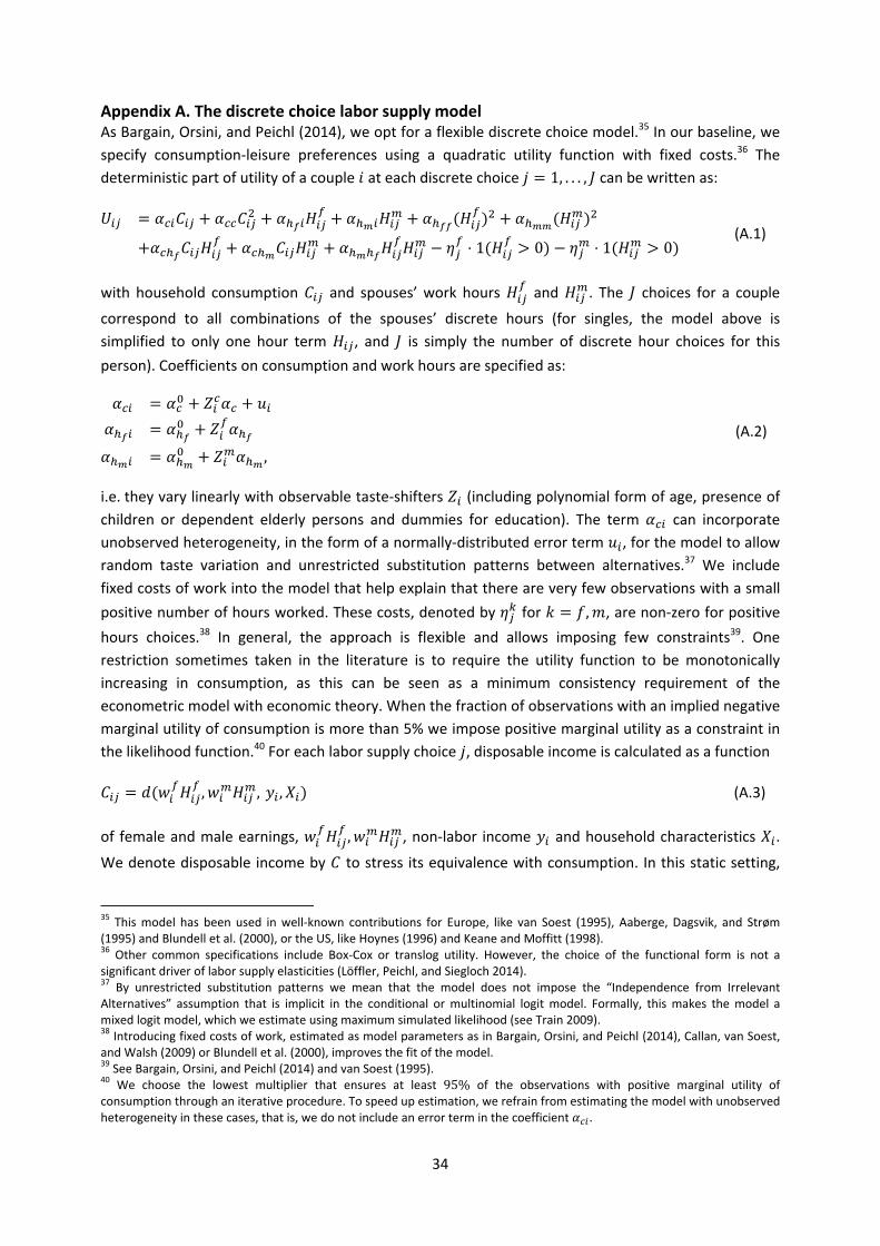
34  

Appendix A. The discrete choice labor supply model As Bargain, Orsini, and Peichl (2014), we opt for a flexible discrete choice model.35 In our baseline, we 

specify  consumption‐leisure  preferences  using  a  quadratic  utility  function  with  fixed  costs.36  The 

deterministic part of utility of a couple   at each discrete choice  1, . . . ,  can be written as:  

⋅ 1 0 ⋅ 1 0               (A.1)  

with household  consumption   and  spouses’ work hours   and  . The    choices  for a  couple 

correspond  to  all  combinations  of  the  spouses’  discrete  hours  (for  singles,  the  model  above  is 

simplified  to only one hour  term  ,  and    is  simply  the number of discrete hour  choices  for  this 

person). Coefficients on consumption and work hours are specified as: 

,

                                                                                                                              (A.2) 

i.e. they vary linearly with observable taste‐shifters   (including polynomial form of age, presence of 

children  or  dependent  elderly  persons  and  dummies  for  education).  The  term    can  incorporate 

unobserved heterogeneity, in the form of a normally‐distributed error term  , for the model to allow 

random  taste  variation  and  unrestricted  substitution  patterns  between  alternatives.37 We  include 

fixed costs of work into the model that help explain that there are very few observations with a small 

positive number of hours worked. These costs, denoted by   for  , , are non‐zero for positive 

hours  choices.38  In  general,  the  approach  is  flexible  and  allows  imposing  few  constraints39.  One 

restriction  sometimes  taken  in  the  literature  is  to  require  the  utility  function  to  be monotonically 

increasing  in  consumption,  as  this  can  be  seen  as  a  minimum  consistency  requirement  of  the 

econometric model with economic theory. When the fraction of observations with an implied negative 

marginal utility of consumption is more than 5% we impose positive marginal utility as a constraint in 

the likelihood function.40 For each labor supply choice  , disposable income is calculated as a function  

, ,   ,                                                                                                                     (A.3) 

of  female and male earnings,  , , non‐labor  income   and household characteristics  . 

We denote disposable  income by   to stress  its equivalence with consumption.  In this static setting, 

                                                            35 This model has been used  in well‐known  contributions  for Europe,  like van Soest  (1995), Aaberge, Dagsvik, and Strøm (1995) and Blundell et al. (2000), or the US, like Hoynes (1996) and Keane and Moffitt (1998). 36 Other  common  specifications  include  Box‐Cox  or  translog  utility. However,  the  choice  of  the  functional  form  is  not  a significant driver of labor supply elasticities (Löffler, Peichl, and Siegloch 2014). 37  By  unrestricted  substitution  patterns  we mean  that  the model  does  not  impose  the  “Independence  from  Irrelevant Alternatives”  assumption  that  is  implicit  in  the  conditional or multinomial  logit model.  Formally,  this makes  the model a mixed logit model, which we estimate using maximum simulated likelihood (see Train 2009). 38 Introducing fixed costs of work, estimated as model parameters as in Bargain, Orsini, and Peichl (2014), Callan, van Soest, and Walsh (2009) or Blundell et al. (2000), improves the fit of the model. 39 See Bargain, Orsini, and Peichl (2014) and van Soest (1995). 40  We  choose  the  lowest  multiplier  that  ensures  at  least  95%  of  the  observations  with  positive  marginal  utility  of consumption through an iterative procedure. To speed up estimation, we refrain from estimating the model with unobserved heterogeneity in these cases, that is, we do not include an error term in the coefficient  . 

 

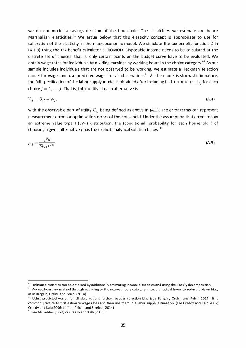
35  

we  do  not  model  a  savings  decision  of  the  household.  The  elasticities  we  estimate  are  hence 

Marshallian  elasticities.41  We  argue  below  that  this  elasticity  concept  is  appropriate  to  use  for 

calibration of  the elasticity  in  the macroeconomic model. We simulate  the  tax‐benefit  function    in 

(A.1.3) using  the  tax‐benefit calculator EUROMOD. Disposable  income needs  to be calculated at  the 

discrete  set  of  choices,  that  is, only  certain points on  the budget  curve have  to be  evaluated. We 

obtain wage rates for individuals by dividing earnings by working hours in the choice category.42 As our 

sample  includes  individuals  that are not observed  to be working, we estimate a Heckman  selection 

model for wages and use predicted wages for all observations43. As the model is stochastic in nature, 

the full specification of the labor supply model is obtained after including i.i.d. error terms   for each 

choice  1, . . . , . That is, total utility at each alternative is 

,                                                                                                                                                 (A.4) 

with the observable part of utility   being defined as above in (A.1). The error terms can represent 

measurement errors or optimization errors of the household. Under the assumption that errors follow 

an  extreme  value  type  I  (EV‐I)  distribution,  the  (conditional)  probability  for  each  household    of 

choosing a given alternative   has the explicit analytical solution below:44 

∑.                                                                                                                                                  (A.5) 

   

                                                            41 Hicksian elasticities can be obtained by additionally estimating income elasticities and using the Slutsky decomposition. 42 We use hours normalized through rounding to the nearest hours category instead of actual hours to reduce division bias,  as in Bargain, Orsini, and Peichl (2014). 43  Using  predicted wages  for  all  observations  further  reduces  selection  bias  (see  Bargain, Orsini,  and  Peichl  2014).  It  is common practice to first estimate wage rates and then use them  in a  labor supply estimation, (see Creedy and Kalb 2005; Creedy and Kalb 2006; Löffler, Peichl, and Siegloch 2014). 44 See McFadden (1974) or Creedy and Kalb (2006). 

 

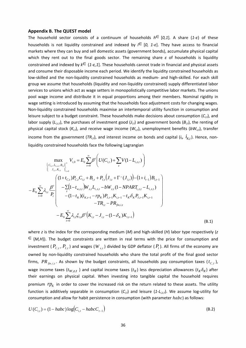
36  

Appendix B. The QUEST model 

The  household  sector  consists  of  a  continuum  of  households  h [0,1].  A  share  (1‐ε)  of  these 

households  is  not  liquidity  constrained  and  indexed  by  i [0,  1‐ε].  They  have  access  to  financial 

markets where they can buy and sell domestic assets (government bonds), accumulate physical capital 

which  they  rent  out  to  the  final  goods  sector.  The  remaining  share  ε  of  households  is  liquidity 

constrained and indexed by k (1‐ε,1]. These households cannot trade in financial and physical assets 

and consume their disposable income each period. We identify the liquidity constrained households as 

low‐skilled and  the non‐liquidity constrained households as medium‐ and high‐skilled. For each  skill 

group we assume that households (liquidity and non‐liquidity constrained) supply differentiated labor 

services to unions which act as wage setters in monopolistically competitive labor markets. The unions 

pool wage  income and distribute  it  in equal proportions among  their members. Nominal  rigidity  in 

wage setting is introduced by assuming that the households face adjustment costs for changing wages. 

Non‐liquidity constrained households maximise an  intertemporal utility function  in consumption and 

leisure subject to a budget constraint. These households make decisions about consumption (Ci,t), and 

labor supply (Li,z,t), the purchases of investment good (Ji,t) and government bonds (Bi,t), the renting of 

physical capital  stock  (Ki,t), and  receive wage  income  (Ws,t), unemployment benefits  (bWs,t),  transfer 

income  from  the government  (TRi,t), and  interest  income on bonds and capital  (it,  tKi , ). Hence, non‐

liquidity constrained households face the following Lagrangian 

1,,,,,0

0

,,,

1,1,1,1,1,

,,,,,,,,,,

1,1,,,,,,,

.0

0

,,,0

00,

,

,,

)1(

))(1(

)1(1

1)()1(

)1()(max

0,,

,,,,

tiKtitit

titit

tifinti

titIKKtitIKtKK

tzitzitztzitztzwz

tittititItititCtC

t

t

tit

tziz

tit

ti

KJ

BLC

KJKE

PRTR

KPtKPrpit

LNPARTbWLWt

BiJJPBCPt

PE

LVCUEV

J

ttiti

titsiti

                                        (B.1) 

where z is the index for the corresponding medium (M) and high‐skilled (H) labor type respectively (z

{M,H}).  The  budget  constraints  are  written  in  real  terms  with  the  price  for  consumption  and 

investment ( tCP , , tIP , ) and wages ( tzW , ) divided by GDP deflator ( tP ). All firms of the economy are 

owned by non‐liquidity  constrained households who  share  the  total profit of  the  final  good  sector 

firms,  tifinPR ,, . As  shown  by  the  budget  constraints,  all  households  pay  consumption  taxes  ( tCt , ), 

wage  income  taxes  ( , ,   ) and capital  income  taxes  ( )  less depreciation allowances  ( ) after 

their  earnings  on  physical  capital.  When  investing  into  tangible  capital  the  household  requires 

premium  Krp   in order  to cover  the  increased  risk on  the  return  related  to  these assets. The utility 

function  is  additively  separable  in  consumption  (Ci,t)  and  leisure  (1‐Li,z,t). We  assume  log‐utility  for 

consumption and allow for habit persistence in consumption (with parameter  ) as follows: 

1,, log)1()( ttiti habcCChabcCU                                                                                                   (B.2) 

 

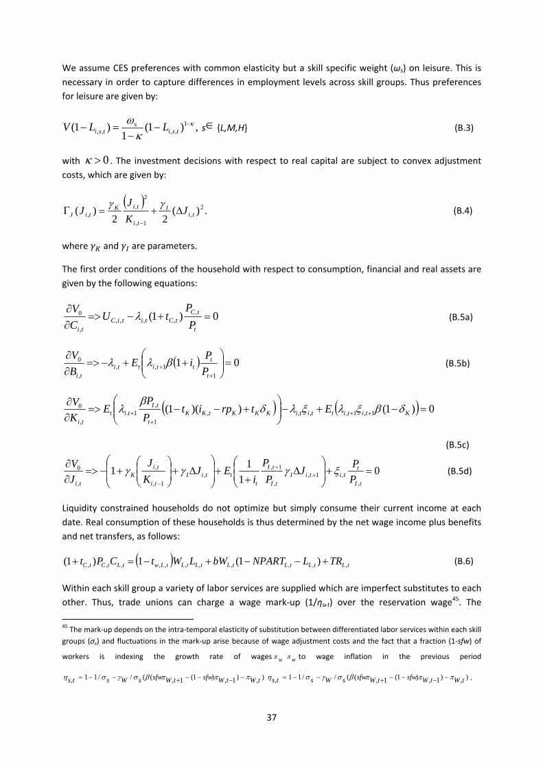
37  

We assume CES preferences with common elasticity but a skill specific weight (ωs) on  leisure. This  is 

necessary  in order to capture differences  in employment  levels across skill groups. Thus preferences 

for leisure are given by: 

,)1(1

)1( 1,,,,

tsis

tsi LLV  s {L,M,H}                                                                                        (B.3) 

with  0 . The  investment decisions with  respect  to  real capital are subject  to convex adjustment 

costs, which are given by:  

.)(

22)( 2

,1,

2

,, ti

I

ti

tiKtiJ J

K

JJ

                                                                                                            (B.4) 

where   and   are parameters. 

The first order conditions of the household with respect to consumption, financial and real assets are 

given by the following equations:  

0)1( ,,,,,

,

0

t

tCtCtitiC

ti P

PtU

C

V                                                                                                     (B.5a) 

011

1,,,

0

t

tttitti

ti P

PiE

B

V                                                                                     (B.5b) 

0)1())(1( 1,1,,,,1

,1.

,

0

KtitittitiKKKtKKt

tItit

ti

EtrpitP

PE

K

V

                                                

                                                                                                                                                                         (B.5c)                            

01

11

,,1,

,

1,,

1,

,

,

0

tI

ttitiI

tI

tI

tttiI

ti

tiK

ti P

PJ

P

P

iEJ

K

J

J

V                            (B.5d) 

Liquidity constrained households do not optimize but  simply consume  their current  income at each 

date. Real consumption of these households is thus determined by the net wage income plus benefits 

and net transfers, as follows: 

tLtLtLtLtLtLtLwtLtCtC TRLNPARTbWLWtCPt ,,,,,,,,,,, )1(1)1(                                              (B.6) 

Within each skill group a variety of labor services are supplied which are imperfect substitutes to each 

other.  Thus,  trade  unions  can  charge  a  wage  mark‐up  (1/ηs,t)  over  the  reservation  wage45.  The 

                                                            45 The mark‐up depends on the intra‐temporal elasticity of substitution between differentiated labor services within each skill 

groups  (σs) and  fluctuations  in  the mark‐up arise because of wage adjustment costs and  the  fact  that a  fraction  (1‐sfw) of 

workers  is  indexing  the  growth  rate  of  wages W

W to  wage  inflation  in  the  previous  period 

),)1,)1(1,((//11, tWtWsfwtWsfwsWsts ),)1,)1(1,((//11, tWtWsfwtWsfwsWsts . 

 

38  

reservation wage is given as the marginal utility of leisure divided by the corresponding marginal utility 

of  consumption.  The  relevant  net  real  wage  to  which  the mark  up  adjusted  reservation  wage  is 

equated  is the gross wage adjusted for  labor taxes, consumption taxes and unemployment benefits, 

which act as a subsidy to leisure. Thus, the wage equation is given as  

},,{for )1(

)1(1

,,

,,,

,,,,

,,,1 HMLstP

btW

U

V

tCtC

tswts

tstshC

tshL

,46                                                                         (B.7) 

where b  is the benefit replacement rate. The aggregate of any household specific variable Xh,t  in per 

capita terms is given by 

tktitht XXdhXX ,,,

1

0

1 .                                                                                                      (B.8) 

Hence, aggregate consumption and employment are given by 

tktit CCC ,,1                                                                                                                                   (B.9) 

and 

.1 ,, tktit LLL                                                                                                                                 (B.10) 

We assume  that  final goods producers work under monopolistic  competition  setting and each  firm 

produces a variety of  the domestic good which  is an  imperfect  substitute  for varieties produced by 

other firms. Final output of firm j ( tjY , ) is produced using capital  tjK ,  and a labor aggregate ( tjL , ) in a 

Cobb‐Douglas technology, subject to a fixed cost  ,.jFC , as follows: 

YjtjtjLjtjtj FCKuFCLY ,

1

,,,,,

                                                                                                                                                (B.11) 

with 

1111111

,,,,,,,

tHjHHtMjMMtLjLLtj LLLL ,                                          (B.12) 

                                                            46 In order to find the wage equation, consider the problem of representative household i, of a subgroup s of the population 

given by (B.1). Then, the first order conditions with respect to labor ( , , ) is the following: 

, ,0 ⇔ 1 , ,

, 1 , , ,                                                                              

We can now combine  the above condition with  the  first order condition with  respect  to consumption, given by condition 

(2.2.5a), to obtain the intra‐temporal condition on the optimal household choices on consumption and labor: 

, ,

,

, , ,

, ,                                                                                                                           

We can recognize in the above condition equation (B.7), which determines the equilibrium wage. In fact, and as mentioned 

before, since within each sub‐group s the  labor services supplied are  imperfect substitutes of each other, the trade unions 

can charge a wage mark‐up (1,) over the reservation wage, which is given by the ratio of the marginal utilities of leisure 

and consumption, i.e. the left‐hand side of the above equation. 

 

39  

where  jtLL , , 

jtML ,   and 

jtHL , denote  the  employment  of  low,  medium  and  high‐skilled  by  firm  j 

respectively. Parameter Λs  is the corresponding share parameter HMLs ,, , χs  is the efficiency 

unit, and µ  is  the elasticity of substitution between different  labor  types. The  term j

LFC represents 

overhead labor and  jtu is the measure of capacity utilisation. The objective of the firm is to maximise 

the present discounted value of profits: 

))(),,()((1 ,,,,,,,,,,,,,,,,,,,, tju

tHjtMjtLjL

tjP

tjtIjKt

stsjtsjtsertjtjtj uLLLPKPiLWtYPPR

                                                                                                                                                                        (B.13) 

where  Ki denotes the rental rate of capital  tsert ,,  stands for the implicit tax rate on labor levied on the 

employers. Following Ratto et al.  (2009), we assume  that  firms  face  technological constraints which 

restrict  their  price  setting,  employment  and  capacity  utilisation  decisions.  These  constraints  are 

captured by the corresponding adjustment costs  )( uLP . It can be shown that in a symmetric 

equilibrium, when  jPP ttj ,, , firms charge a mark‐up over the marginal cost of production (MC): 

tjtj

tj MCP ,,

,

1

                                                                                                                                (B.14) 

where  tj ,   is  the  inverse  price mark‐up  factor which  is  defined  as  a  function  of  the  elasticity  of 

substitution  ( d ),  changes  in  inflation  ( )  and  the  mark‐up  shock  ( mkp )47.  Skill‐specific  labor 

demand can be obtained from the first order condition with respect to labor: 

HMLsL

LLLWt

L

YP

jtsj

tHjtMjtLjL

tstsertjtsj

tjtj ,,,

),,(1

,,

,,,,,,,,,,

,,

,,

,                             (B.15) 

where  the marginal  product  of  labor,  the  corresponding  adjustment  costs  and  the  gross mark‐up 

factor will jointly determine the optimally chosen level of low‐, medium‐ and high‐skilled employment 

level. Similarly, the demand for capital is constrained by the corresponding first order condition:  

tIjtKtjtj

tjtj Pi

K

YP ,,,,

,

,,1

                                                                                                                  (B.16) 

where  tIjP ,,   is  the price of  investment goods while  tKi ,   is  the rental rate of capital. Finally,  the  first 

order condition for capacity utilisation is: 

tIjtKtjtjtj

tjtj Pi

ucapK

YP ,,,,

,,

,,1

                                                                                                   (B.17) 

                                                            47 We  follow Ratto et al.  (2009) and allow  for additional backward  looking elements by assuming that a  fraction (1−sfp) of 

firms index price increases to inflation in t−1, mkpttsfpttsfpEPd

tj 111/11, , where  P P is 

the corresponding adjustment cost parameter. 

 

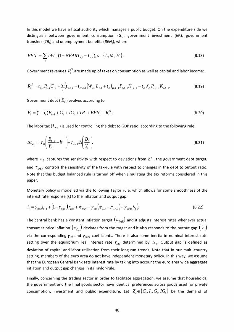
40  

In this model we have a fiscal authority which manages a public budget. On the expenditure side we 

distinguish  between  government  consumption  (Gt),  government  investment  (IGt),  government 

transfers (TRt) and unemployment benefits (BENt), where 

HMLsLNPARTbWBEN tststss

t ,,),1( ,,, .                                                                       (B.18) 

Government revenues GtR  are made up of taxes on consumption as well as capital and labor income: 

.1,1,1,1,1,,,,,,,,,, titIKKtitItKKtststsertsws

titCtCGt KPtKPitLWttCPtR                        (B.19) 

Government debt ( tB ) evolves according to 

.)1( 1Gtttttttt RBENTRIGGBiB                                                                        (B.20) 

The labor tax ( twt , ) is used for controlling the debt to GDP ratio, according to the following rule: 

,1

1,

t

tDEF

T

t

tBtw Y

Bb

Y

Bt                                                                                                     (B.21) 

where  B  captures the sensitivity with respect to deviations from  Tb , the government debt target, 

and  DEF  controls the sensitivity of the tax‐rule with respect to changes  in the debt to output ratio. 

Note that this budget balanced rule  is turned off when simulating the tax reforms considered  in this 

paper. 

Monetary policy  is modelled via the following Taylor rule, which allows for some smoothness of the 

interest rate response (it) to the inflation and output gap: 

.1 ,inf1 tygapTARtCTAREQilagtilagt yrii                                                        (B.22) 

The central bank has a constant  inflation target  TAR  and  it adjusts  interest rates whenever actual 

consumer price inflation  tC ,  deviates from the target and it also responds to the output gap  ty

 

via  the  corresponding  γinf  and  γygap  coefficients.  There  is  also  some  inertia  in nominal  interest  rate 

setting  over  the  equilibrium  real  interest  rate  EQr   determined  by  γilag.  Output  gap  is  defined  as 

deviation of  capital and  labor utilisation  from  their  long  run  trends. Note  that  in our multi‐country 

setting, members of the euro area do not have independent monetary policy. In this way, we assume 

that the European Central Bank sets interest rate by taking into account the euro area wide aggregate 

inflation and output gap changes in its Taylor‐rule. 

Finally, concerning  the  trading sector  in order  to  facilitate aggregation, we assume  that households, 

the government and the  final goods sector have  identical preferences across goods used  for private 

consumption,  investment  and  public  expenditure.  Let  ttttt IGGICZ ,,,   be  the  demand  of 

 

41  

households,  investors or  the government as defined  in  the previous section. Then  their preferences 

are given by the following utility function: 

1

11

,

1

,

1

1

im

im

im

im

imim

im

im tftdt ZZZ

,                                                                                     (B.23) 

where  is the share parameter and σim  is the elasticity of substitution between domestic  (Zd,t) and 

foreign produced goods (Zf,t). 

   

 

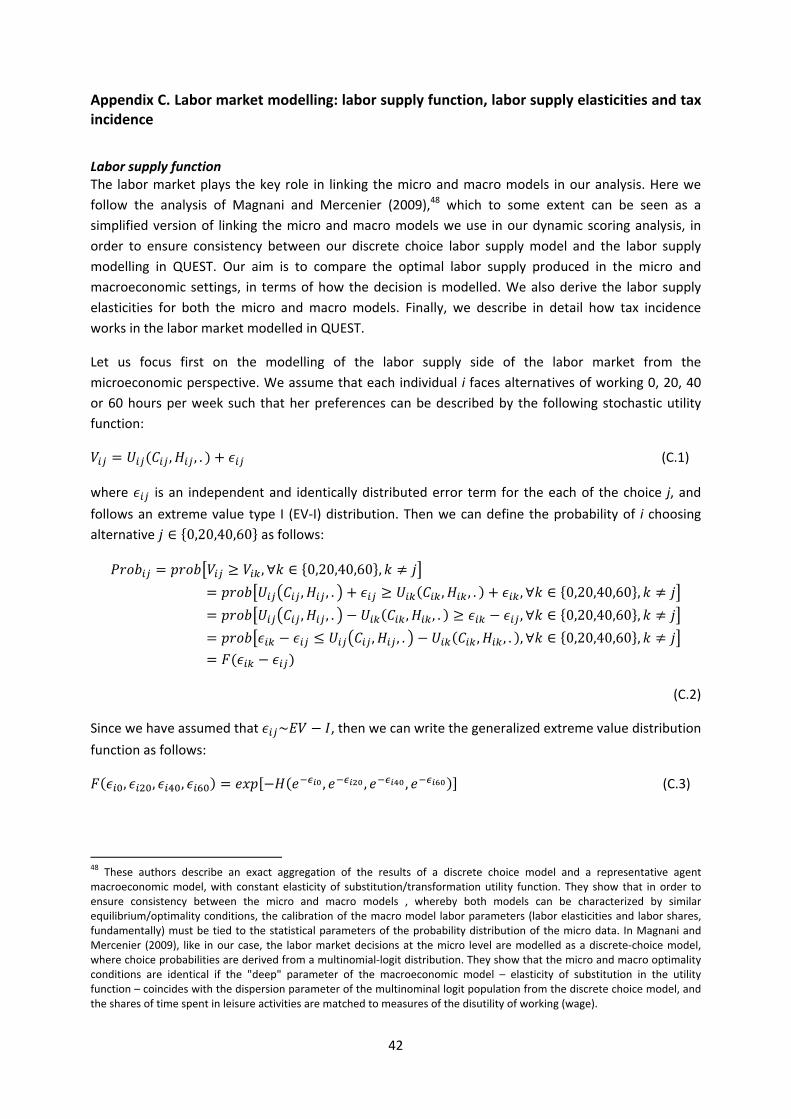
42  

Appendix C. Labor market modelling: labor supply function, labor supply elasticities and tax incidence  

Labor supply function The  labor market plays the key role  in  linking the micro and macro models  in our analysis. Here we 

follow  the  analysis  of Magnani  and Mercenier  (2009),48  which  to  some  extent  can  be  seen  as  a 

simplified version of  linking  the micro and macro models we use  in our dynamic scoring analysis,  in 

order  to  ensure  consistency between our discrete  choice  labor  supply model  and  the  labor  supply 

modelling  in QUEST.  Our  aim  is  to  compare  the  optimal  labor  supply  produced  in  the micro  and 

macroeconomic settings,  in  terms of how  the decision  is modelled. We also derive  the  labor supply 

elasticities  for  both  the micro  and macro models.  Finally, we  describe  in  detail  how  tax  incidence 

works in the labor market modelled in QUEST. 

Let  us  focus  first  on  the  modelling  of  the  labor  supply  side  of  the  labor  market  from  the 

microeconomic perspective. We assume that each  individual  i faces alternatives of working 0, 20, 40 

or 60 hours per week such  that her preferences can be described by  the  following stochastic utility 

function: 

, , .                                                                                                                               (C.1) 

where    is an  independent and  identically distributed error  term  for  the each of  the choice  j, and 

follows an extreme value  type  I  (EV‐I) distribution. Then we can define  the probability of  i choosing 

alternative  ∈ 0,20,40,60  as follows: 

, ∀ ∈ 0,20,40,60 ,

, , . , , . , ∀ ∈ 0,20,40,60 ,

, , . , , . , ∀ ∈ 0,20,40,60 ,

, , . , , . , ∀ ∈ 0,20,40,60 ,

 

     (C.2) 

Since we have assumed that  ~ , then we can write the generalized extreme value distribution 

function as follows: 

, , , , , ,                                                               (C.3) 

                                                            48  These  authors  describe  an  exact  aggregation  of  the  results  of  a  discrete  choice  model  and  a  representative  agent macroeconomic model, with constant elasticity of  substitution/transformation utility  function. They  show  that  in order  to ensure  consistency  between  the  micro  and  macro  models  ,  whereby  both  models  can  be  characterized  by  similar equilibrium/optimality conditions, the calibration of the macro model  labor parameters (labor elasticities and  labor shares, fundamentally) must be tied to the statistical parameters of the probability distribution of the micro data.  In Magnani and Mercenier  (2009),  like  in our case,  the  labor market decisions at  the micro  level are modelled as a discrete‐choice model, where choice probabilities are derived from a multinomial‐logit distribution. They show that the micro and macro optimality conditions  are  identical  if  the  "deep"  parameter  of  the macroeconomic model  –  elasticity  of  substitution  in  the  utility function – coincides with the dispersion parameter of the multinominal logit population from the discrete choice model, and the shares of time spent in leisure activities are matched to measures of the disutility of working (wage).  

 

43  

Function H satisfies all the necessary conditions to ensure that F is a cumulative distribution function. 

Following Magnani and Mercenier (2009), we assume that the following functional form for  is: 

, , , ∑ ∈ , , ,                                                                                                 (C.4) 

Given the functional form of H, then the cumulative distribution F  is equal to the product of double 

exponential distributions  that characterize  the behavior of    for each alternative of working hours 

such that: 

, , , ∑ ∈ , , , ∑ ∈ , , ,                          (C.5)                            

and F assumes the following form: 

, , , ∑ ∈ , , , ∏ ∈ , , ,                (C.6) 

Then, according to McFadden theorem, the probability of i choosing alternative j is given by: 

, , ,                                                                                                              (C.7) 

where   is the dispersion parameter of the extreme value distribution. The probability we are looking 

for can be obtained by substituting (C.5) into (C.7) to obtain: 

∑ ∈ , , ,

                                                                                                                                (C.8) 

which, when  1, is equivalent to : 

∑ ∈ , , ,.                                                                                                                                  (C.9) 

Then, the expected number of hours supplied by individual i will be given by: 

∑ ∈ , , , ∗ ∑∑ ∈ , , ,

∈ , , , ∗∑ ∗∈ , , ,

∑ ∈ , , ,                        (C.10) 

Consider now  that  a  given  individual  i belongs  to  a particular  sub‐population  group  that  share  the 

same  socio‐economic  characteristics,  and  that  there  are  N  statistically  identical  and  independent 

individuals  in  this  sub‐population  group.  Then,  within  this  group,  the  expected  number  of  hours 

supplied will be given by: 

∑ ∑∑ ∗∈ , , ,

∑ ∈ , , ,                                                                                                          (C.11) 

Note that equation (C.11) is a simplified analytical expression of the labor supply function for a group 

of  individuals  sharing  the  same  socio‐economic  characteristics. We  can  also  compute  the expected 

number  of  individuals  in  this  population  subgroup  that  will  choose  any  of  the  working  hours' 

alternatives.  For  instance,  the expected number of  individuals  supplying  zero hours,  i.e.  individuals 

deciding not to participate in the labor market, is equal to: 

 

44  

∗∑ ∈ , , ,

∗                                                                                                (C.12) 

Similarly,  the  expected  number  of working  individuals,  i.e.  individuals  supplying  non‐zero working 

hours, is equal to: 

1 ∗ 1∑ ∈ , , ,

∗                                                       (C.13) 

In more general terms, the expected number of individuals choosing any alternative j of the setting of 

alternatives is equal to: 

∗∑ ∈ , , ,

∗                                                                                                     (C.14) 

We turn now to the macroeconomic setting. In QUEST the labor market is populated by workers, and 

firms. The QUEST model therefore takes into account both the supply and demand of labor. Focusing 

only  on  the  partial  equilibrium,  this  translates  into  a  system  of  equations  that  allows  finding  the 

equilibrium wage  and working  hours.  In  this way,  and  abstracting  from  other  general  equilibrium 

effects, the referred system is presented below:49 

)1(

)1(1

,,

,,,

,,,,

,,,1

tCtC

tswts

tstshC

tshL

tP

btW

U

V

j

tsj

tHjtMjtLjL

tstsertjtsj

tjtj L

LLLWt

L

YP

,,

,,,,,,,,,,

,,

,,

),,(1

 

)1(

)1(1

,,

,,,

,,,,

,,,1

tCtC

tswts

tstshC

tshL

tP

btW

U

V

j

tsj

tHjtMjtLjL

tstsertjtsj

tjtj L

LLLWt

L

YP

,,

,,,,,,,,,,

,,

,,

),,(1

, ,                            

(C.15) 

where  the  first  equation  of  the  system50  results  from  the  combination  between  the  first  order 

conditions with respect to consumption and  labor –  i.e.  is the  inter‐temporal and the  intra‐temporal 

optimality conditions, respectively – resulting from the household problem, and the second equation 

of the system results from maximizing firms profits with respect to labor.51 From the system in (C.15), 

we  obtain  the  partial  equilibrium  pair  of  hours  worked  and  wage  rate ,∗ , ,

∗ , ∈ , ,   . 

Notice that the decisions modelled in the supply side of the labor market have similar aspects in both 

micro and macro settings: both consider maximization of individual/household utilities, which depend 

on  consumption  and  leisure.  However,  in  the  macro  setting,  the  number  of  hours  worked  in 

equilibrium is derived from intersecting labor supply and labor demand functions, i.e. QUEST take into 

                                                            49 Note that QUEST  is characterized by the system of all the equilibrium conditions of economic agents,  laws of motion of state endogenous variables and shocks, and feasibility conditions, and as such the solution of the model implies solving this system, and having all the (approximated) conditions met simultaneously in the steady state. 50 This corresponds to equation B.7 in Appendix B. 51 This corresponds to equation B.15 in Appendix B. 

 

45  

account the demand of labor. This demand effect, which is basically constrained by the labor demand 

elasticity to wages, is not considered in the micro framework but rather taken as given by the macro‐

economic conditions described by the DSGE model.52 Considering the following functional form of the 

household utility  function  in QUEST, given by expressions  (C.16) and  (C.17) below  53,  for  skill group 

∈ , , , 

, , ,, ,

, ∈ , ,                                                                                                                (C.16) 

and, 

, , ,,

, ∈ , ,                                                                                                             (C.17) 

and  substituting  them  in  the  inter‐temporal  condition  of  the  system  in  (C.15),  we  obtain  the 

expression for the labor supply function in QUEST: 

, , 1,

, , ,

, , ,⇔ , , 1

, , , ,

, ,

, , ,                                 

                                                                                                                                                                              (C.18) 

If we  now  consider  that  there  are N  identical  households  on  the  skill  group  ∈ , ,  we  can 

rewrite (C.18) as follows: 

, 1, , , ,

, ,

, , ,                                                                                       (C.19) 

Expression  (C.19) can be compared with expression  (C.13),  the expected number of  individuals  that 

was  derived  in  our  simplified  discrete  choice  setting.  First  of  all,  notice  that  both  expressions  are 

optimality  conditions  derived  from  a  utility maximization  problem,  conditional  on  how much  the 

household wants  to  consume.  To  see  this  better, we  can write  expression  (C.19)  in  the  following 

terms: 

, 1 ; Τ ; Ω                                                                                                                              (C.20) 

where  g(.)  is  a  function  of  a  vector  of  aggregated  endogenous  variables,  ,  a  vector  of  policy 

exogenous  variables,  ,  and  a  vector  of  parameters,  Ω,  ,  with  , , , , , ; , ;

, , , , , ; Ω , , .  

In a similar way, we can rewrite (C.13) as follows: 

1 ; Θ                                                                                                                               (C.21) 

where F(.) is the distribution function depending on the arguments of the deterministic utility function 

, ,   and  on  a  set  of  parameters  Θ.  However, while  expression  (C.19)  denotes  the 

                                                            52 Notice that not considering labor demand in the micro model can be problematic in what concerns the coherence between the micro and macro settings. It may be difficult to obtain convergence on the main economic aggregates between the two models.  53 These correspond to expressions B.2 and B.3 in Appendix B. 

 

46  

optimal amount of labor services supplied, in terms of total number of hours, for any level of the net 

adjusted wage –  intensive margin –, expression  (C.13) denotes  the expected number of  individuals 

working  in  the economy – extensive margin. Furthermore, notice  that,  in QUEST, unemployment  is 

obtained endogenously and is equal to: 

1 , ,                                                                                                                 (C.22) 

where NPART is the non‐participation rate. In QUEST households only decide on the amount of hours 

supplied in the labor market, but they do not choose between unemployment and non‐participation, 

explicitly. The non‐participation rate is calibrated as the proportion of inactive in the total population. 

The  non‐participation  rate  (NPART)  must  therefore  be  seen  as  an  exogenous  policy  variable 

characterising the generosity of the benefit system. However, in our discrete choice model the choice 

of non‐participation, or being unemployed voluntarily, is one of the possible alternatives of individual 

i. The  choice of participating  in  the  labor market  is nested  together with  the decision on  supplying 

different number of hours (which can be seen as the different working modalities). We reconcile the 

two models on this issue by calibrating in QUEST the non‐participation rate according to the expected 

number of  individuals that choose to be out of the  labor market,  i.e. equation (C.12)  in the discrete 

choice model. 

Labor market elasticities In our dynamic  scoring exercise,  labor market elasticities are  crucial  to understand  the effects of a 

particular tax reforms on the households' disposable  income,  in particular, and on the economy as a 

whole. More specifically, the  labor supply elasticity  is a good measure of the work effort  incentives, 

and,  in  this way,  crucial  to understand  the effects of  the  tax  reforms  implemented on  the workers 

behavior. Moreover, the analysis of the elasticities in both models is important to see whether we can 

calibrate QUEST with  the elasticities obtained  from our microeconometric model,  so  that a greater 

consistency can be achieved in linking the two models. In what follows we derive analytically the labor 

supply elasticities in the micro and macro settings, and see how these relate to each other. Recall that 

in what concerns QUEST, the parameter that we are interested in calibrating is the parameter  .54 This 

parameter relates the Frisch elasticity to the inter‐temporal elasticity of substitution, as we will see in 

what follows. 

In QUEST, the Frisch elasticity  is defined as the elasticity of the  labor supply, as defined  in equation 

(C.19), with respect to the wage, maintaining the marginal utility of consumption constant. In this way, 

we can define the Frisch elasticity as follows: 

,

,,

,,

,,

,                                                                                                      (C.23) 

The elasticity in (C.23) suggests a positive relationship between wages and labor supply, depending on 

the level of labor hours supplied. This implies that the Frisch elasticity might differ (and, in fact, it will) 

for the three skill groups considered in QUEST. In this way, we expect that some groups will be more 

reactive  to  changes  in  the wage  level  than others. Besides  the  Frisch  elasticity,  another  important 

                                                            54 Please check the functional form given in expression (B.3) in Appendix B. 

 

47  

result  in  macroeconomic  models  such  as  QUEST  is  how  labor  supply  evolves  over  time,  given 

temporary changes  in the wages path. This  is known as  the  inter‐temporal elasticity of substitution, 

.  In  this way,  this  elasticity measures  the  relation  between  the  changes  in  the  ratio  of  labor 

supplied tomorrow and today, and the ratio of wages paid tomorrow and today. In order to derive this 

elasticity, we need to find the  inter‐temporal  labor supply function, where we can relate the path of 

labor  supply with  the path of wages.  For  that  consider  the QUEST model described  in Appendix B. 

Consider also the labor supply function in equation (C.19) of this appendix section. In order to derive 

the  inter‐temporal  labor  supply  function,  one  needs  to  combine  the  intra‐temporal  optimality 

condition with  the  inter‐temporal one  (the Euler equation).  Let us  consider  first  the  intra‐temporal 

optimality condition given by equation (B.7) and write it one period ahead, as follows: 

, , ,

, , , ,

, , ,

, ,                                                                                                             (C.24) 

From  this  condition we  can  obtain  the  labor  supply  function  of  the  households  in  group  ,  one 

period ahead: 

, 1, , , ,

, ,

, , ,                                                                     (C.25) 

We can now substitute  in  (C.25)  the marginal utility of consumption  , , ,  by  its expression one 

period ahead, given the functional form in expression (B.2): 

, 1, , , ,

, ,,                                    (C.26) 

At  this  point,  we  need  to  consider  also  the  intertemporal  optimality  condition  of  the  household 

problem – the Euler equation. This condition is obtained by combining the first order conditions with 

respect  to  consumption  and  bonds  of  the  household  problem,  i.e.  equations  (B.5a)  and  (B.5b)  in 

Appendix  B  respectively,  and  it  explains  the  path  of  consumption  over  time.  From  these  two 

conditions, we obtain an expression for the Lagrangian multiplier,  , : 

,,

, ,

,                                                                                                                                                   (C.27) 

And writing (C.27) one period ahead, we get: 

,,

, ,

,                                                                                                                                        (C.28) 

Now that we have the expressions of the Lagrangian multiplier, at t and t+1, we can substitute them in 

the first order condition with respect to bonds to obtain the Euler equation: 

, ,

, ,

, ,

, ,                                                                                                          (C.29) 

where we can explicitly  include  the expressions of  the marginal utility of consumption at  t and  t+1. 

Then, the Euler equation can be re‐written as follows: 

, 1 , , 1 , 1 , ,                      (C.30) 

 

48  

The next step is to include the Euler equation derived in equation (C.30) in the labor supply function, 

equation (C.26) to obtain a relation between the labor supplied tomorrow and consumption today, as 

follows: 

, 1, , , ,

, , ,                                     (C.31) 

Recurring again  to  the  intra‐temporal optimality condition, and  substituting  the marginal utilities of 

leisure and consumption, we find that: 

, 1 , ,,

, 1 , , 1 , ,                                 (C.32) 

Substituting the previous result in the labor supply equation given by (C.31), we will obtain finally an 

expression which includes  , , , , , , and  , , shown below. 

, 1 ,

,

, , ,

, , ,1 1 , ,                                                   (C.33) 

After some algebraic computations we can derive the following expression, which relates the path of 

leisure hours (and labor supply) with the path of wages, as follows: 

, ,

, ,1 ,

,

, ,

, ,

,

,                                                                           (C.34) 

Similarly to the Euler equation, equation (C.34) represents the inter‐temporal optimality condition for 

leisure (labor). We can now denote  , ,

, ,1 ,  and  ,

, and rewrite equation (C.34) 

as follows: 

1 , 1 ,

,

, ,

, ,                                                                             (C.35) 

We can now compute the elasticity of inter‐temporal substitution for leisure since the results are very 

easily extrapolated in terms of labor supply. We apply logarithms to equation (C.35) and then compute 

the  derivative  of  the 1 ,   with  respect  to  .  In  this  way,  we  obtain  the  following 

expression: 

1 , 1 ,

,

, ,

, ,,                                                                 (C.36) 

and  

,

,

,

,

,

,

,

                                                        (C.37) 

As  we  can  observe  from  expression  (C.37),  parameter    guides  the  elasticity  of  inter‐temporal 

substitution, and the smaller this parameter is, the higher (in absolute terms) is this elasticity, and the 

more willing  is  the household  to  change  the path of  leisure  (or  labor), given  temporary  changes  in 

 

49  

wages. Moreover, we  can  see  clearly  that  the  relation between  the  Frisch  elasticity  and  the  inter‐

temporal  elasticity  of  substitution  depends  on  the  parameter  .  In  this way, we  can  establish  the 

following relation between the two elasticities: 

, ,,

,                                                                                                                                   (C.38) 

In  the  nonlinear  discrete  choice  econometric  model,  labor  supply  elasticities  cannot  be  derived 

analytically.  However,  using  the  estimated  structural  utility  function,  we  can  calculate  choice 

probabilities for varying incomes. Wage elasticities are calculated after simulating a marginal increase 

in  the  wage  rate  and  predicting  the  probability  distribution  over  the  choice  categories  for  the 

increased wage rate. The wage elasticity  is defined as the change  in expected working hours (that  is, 

the  probability‐weighted  average  of working  hours) with  respect  to  the  change  in  the wage  rate. 

Similarly, we calculate expected  incomes, benefits, and tax payments before and after the simulated 

income change. In this way, using the estimated structural utility function, we predict the probability 

distribution over the hour's categories that emerge after simulating a marginal  increase  in the wage 

rates.  As  the  estimated  utility  function  depends  on  the  net  income,  the  predicted  probability 

distribution will change after the simulated income change. Recall from equation (C.10) the expected 

hours  supplied by household  i. Denote by  the predicted utility of  the household  from working  j 

hours at the marginally increased wage rate. Then expected hours for the new wage can be calculated 

in the same way:  

∑ ∗∈ , , ,

∑ ∈ , , ,∑ ∈ , , , ∗ .                                                                                    (C.39) 

The  labor  supply  elasticity  can be  calculated  as  the  change  in  predicted  hours with  respect  to  the 

marginal change in the wage rate: 

,                                                                                                                              (C.40) 

The econometric framework from which the elasticity is calculated is static in nature. We rely on cross 

sectional data and do not observe households at multiple points in time. Moreover, the econometric 

model  does  not  encompass  saving  decisions.  The  elasticities  we  estimate  are  uncompensated  – 

Marshallian  –  elasticities.  The  Marshallian  elasticity  is  related  by  the  Slutsky  equation  to  the 

compensated  – Hicksian Hicksian)  income  elasticity.  In  studies  focusing  on  the  deadweight  loss  of 

taxation  or  steady  state  responses  to  tax  changes,  the Hicksian  elasticity  is  the  crucial  parameter. 

However,  these studies usually assume  that  tax  revenue  is  redistributed as a  lump sum payment  to 

households,  shutting off  the  income effect. As we do not make  this  assumption,  tax  changes have 

income effects, and  the Marshallian elasticity  is  the appropriate parameter  to use.  In principle, we 

could obtain the Hicksian elasticity as the residual of the Marshallian elasticity (the one we estimate) 

 

50  

and  the  income  effect  (which  we  could  calculate  by  simulating  a marginal  increase  in  non‐labor 

income) but since we focus on a situation with income effects, we refrain from doing so.55 

Comparing the elasticities defined both in the micro and in macroeconomic settings, we conclude that, 

in fact, the elasticity defined in (C.40) is the micro‐equivalent to the elasticity derived in (C.23), i.e. the 

Frisch elasticity, in the macro setting. This is a very important result, because we can greatly improve 

the  consistency  between  the  two models  by  calibrating  the  Frisch  elasticity with  the  labor  supply 

elasticities  estimated  from  the  discrete  choice model.  In  this way,  parameter    in QUEST  can  be 

obtained from the following expression: 

,

,

,                                                                                                                                                    (C.41) 

where  , , . 

Tax incidence in QUEST For  our  exercise  is  very  important  to  assess  how  the  tax  incidence mechanism works  in  the  labor 

market defined in the QUEST model. In this way, following Fullerton and Metcalf (2002) analysis of tax 

incidence and considering the labor market of the QUEST model, workers face the statutory burden of 

paying the fraction   of the gross wage, receiving the net wage defined as follows (for simplicity we 

abstract here from time and skill type indices): 

1                                                                                                                                             (C.42) 

The firms pay gross wages and social insurance contributions, i.e. a total compensation of employees 

defined by: 

1                                                                                                                                              (C.43) 

where    is the gross wage, facing,  in this way, the statutory tax rate of  . However, the economic 

incidence of these taxes may be different from their legal incidence, and this will basically depend on 

the labor supply and demand elasticities with respect to wages. As in Fullerton and Metcalf (2002), let 

us define labor supply elasticity with respect to net wage as follows: 

≅ ,                                                                                          (C.44) 

where  the  symbol  ^  represents  percent  changes.  The  changes  in  labor  supply will  depend  on  the 

changes on gross wages, taxes and on the elasticity parameter as follows: 

                                                                                                                                            (C.45) 

In  the  same way, we  can define  labor demand elasticity with  respect  to  the  total  compensation of 

employees as follows: 

                                                            55 Note that Bargain et al. (2014) estimate uncompensated, income and compensated elasticities using EUROMOD. They find that income effects are almost zero and hence the difference between compensated and uncompensated elasticities is small. 

 

51  

≅                                                                                            (C.46) 

and  the  changes  in  labor  demand will  depend  equally  on  gross wages,  taxes  and  on  the  elasticity 

parameter as follows: 

                                                                                                                                           (C.47) 

Tax changes will lead to a new equilibrium in the labor market, which implies that: 

   .                                                                                                                                                            (C.48) 

Substituting (C.45) and (C.47) into (C.48), we find that, in order to reach the new equilibrium, changes 

in gross wages will be given by the following expression: 

.                                                                                                                        (C.49) 

Since  in QUEST, 0 ∞ and  0, the final change  in the equilibrium wage will depend on 

the relative magnitude of the elasticities and the signs and magnitude of the fiscal policy shocks, i.e., 

the relative changes in   and  . In the same way, we can also find the changes in the net wages and 

total compensation of employees, given  the changes  in  the  tax  rates  for employees and employers. 

Consider the definition of net wages in (C.41). Applying logarithms and differentiating, we obtain: 

 .                                                                                                                                               (C.50) 

Substituting (C.49) in (C.50), we obtain that: 

                                                                                                                                (C.51) 

The ratio    is negative. This means that there  is an  inverse relationship between the change  in 

total  taxes on  labor and net wages. The  same algebraic  reasoning can be done  in order  to  find  the 

change  in  the  total  compensation  of  employees.  Consider  in  this  case  the  definition  of  the  total 

compensation in (C.43). Applying logarithms and differentiating, we obtain: 

 .                                                                                                                                                (C.52) 

Substituting (C.49) in (C.52), we obtain that: 

                                                                                                                                  (C.53) 

The ratio   is positive. This means that there is a direct relationship between the change in total 

taxes  on  labor  and  the  total  compensation.  As we  can  conclude,  tax  incidence  in QUEST,  i.e.  the 

sharing of the tax burden between workers and firms, will depend on the sign and magnitude of the 

elasticities of supply and demand.  

 

 

52  

Appendix D. QUEST impulse responses D.1 Net real wage of employees, per skill level (% quarterly change from baseline) – Reform on employees contributions 

 

0

0,5

1

1,5

2

2,5

3

3,5

1 2 3 4 5 6 7 8 9 10

High skilled

0

0,5

1

1,5

2

2,5

3

3,5

1 2 3 4 5 6 7 8 9 10

High skilled

0

0,5

1

1,5

2

2,5

3

3,5

4

1 2 3 4 5 6 7 8 9 10 11 12

Medium skilled

0

0,5

1

1,5

2

2,5

3

3,5

4

1 2 3 4 5 6 7 8 9 10 11 12

Medium skilled

0

0,5

1

1,5

2

2,5

3

3,5

4

1 2 3 4 5 6 7 8 9 10

Low skilled

0

0,5

1

1,5

2

2,5

3

3,5

4

1 2 3 4 5 6 7 8 9 10

Low skilled

 

53  

D.2 Total compensation of employees, per skill level (% quarterly change from baseline) – Reform on employees contributions 

 

 

 

‐0,7

‐0,6

‐0,5

‐0,4

‐0,3

‐0,2

‐0,1

0

1 2 3 4 5 6 7 8 9 10

High skilled

‐0,7

‐0,6

‐0,5

‐0,4

‐0,3

‐0,2

‐0,1

0

1 2 3 4 5 6 7 8 9 10

High skilled‐0,7

‐0,6

‐0,5

‐0,4

‐0,3

‐0,2

‐0,1

0

1 2 3 4 5 6 7 8 9 10 11 12

Medium skilled

‐0,7

‐0,6

‐0,5

‐0,4

‐0,3

‐0,2

‐0,1

0

1 2 3 4 5 6 7 8 9 10 11 12

Medium skilled

‐0,6

‐0,5

‐0,4

‐0,3

‐0,2

‐0,1

0

1 2 3 4 5 6 7 8 9 10 1

Low skilled

‐0,6

‐0,5

‐0,4

‐0,3

‐0,2

‐0,1

0

1 2 3 4 5 6 7 8 9 10 1

Low skilled

 

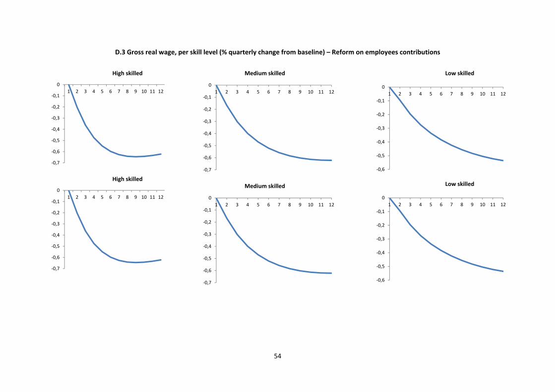
54  

D.3 Gross real wage, per skill level (% quarterly change from baseline) – Reform on employees contributions 

 

 

 

‐0,7

‐0,6

‐0,5

‐0,4

‐0,3

‐0,2

‐0,1

0

1 2 3 4 5 6 7 8 9 10 11 12

High skilled

‐0,7

‐0,6

‐0,5

‐0,4

‐0,3

‐0,2

‐0,1

0

1 2 3 4 5 6 7 8 9 10 11 12

High skilled

‐0,7

‐0,6

‐0,5

‐0,4

‐0,3

‐0,2

‐0,1

0

1 2 3 4 5 6 7 8 9 10 11 12

Medium skilled

‐0,7

‐0,6

‐0,5

‐0,4

‐0,3

‐0,2

‐0,1

0

1 2 3 4 5 6 7 8 9 10 11 12

Medium skilled

‐0,6

‐0,5

‐0,4

‐0,3

‐0,2

‐0,1

0

1 2 3 4 5 6 7 8 9 10 11 12

Low skilled

‐0,6

‐0,5

‐0,4

‐0,3

‐0,2

‐0,1

0

1 2 3 4 5 6 7 8 9 10 11 12

Low skilled

 

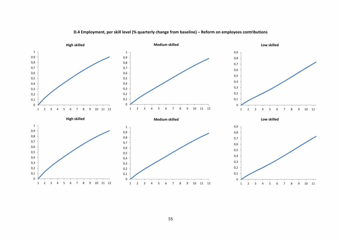
55  

D.4 Employment, per skill level (% quarterly change from baseline) – Reform on employees contributions 

 

0

0,1

0,2

0,3

0,4

0,5

0,6

0,7

0,8

0,9

1

1 2 3 4 5 6 7 8 9 10 11 12

High skilled

0

0,1

0,2

0,3

0,4

0,5

0,6

0,7

0,8

0,9

1

1 2 3 4 5 6 7 8 9 10 11 12

High skilled

0

0,1

0,2

0,3

0,4

0,5

0,6

0,7

0,8

0,9

1

1 2 3 4 5 6 7 8 9 10 11 12

Medium skilled

0

0,1

0,2

0,3

0,4

0,5

0,6

0,7

0,8

0,9

1

1 2 3 4 5 6 7 8 9 10 11 12

Medium skilled

0

0,1

0,2

0,3

0,4

0,5

0,6

0,7

0,8

0,9

1 2 3 4 5 6 7 8 9 10 11

Low skilled

0

0,1

0,2

0,3

0,4

0,5

0,6

0,7

0,8

0,9

1 2 3 4 5 6 7 8 9 10 11

Low skilled

 

56  

D.5 Net real wage of employees, per skill level (% quarterly change from baseline) – Reform on employers contributions 

 

 

0

0,5

1

1,5

2

2,5

3

1 2 3 4 5 6 7 8 9 10 11 12

High skilled

0

0,5

1

1,5

2

2,5

3

1 2 3 4 5 6 7 8 9 10 11 12

High skilled

0

0,5

1

1,5

2

2,5

3

3,5

4

1 2 3 4 5 6 7 8 9 10 11 12

Medium skilled

0

0,5

1

1,5

2

2,5

3

3,5

4

1 2 3 4 5 6 7 8 9 10 11 12

Medium skilled

0

0,5

1

1,5

2

2,5

3

3,5

4

1 2 3 4 5 6 7 8 9 10 11

Low skilled

0

0,5

1

1,5

2

2,5

3

3,5

4

1 2 3 4 5 6 7 8 9 10 11

Low skilled

 

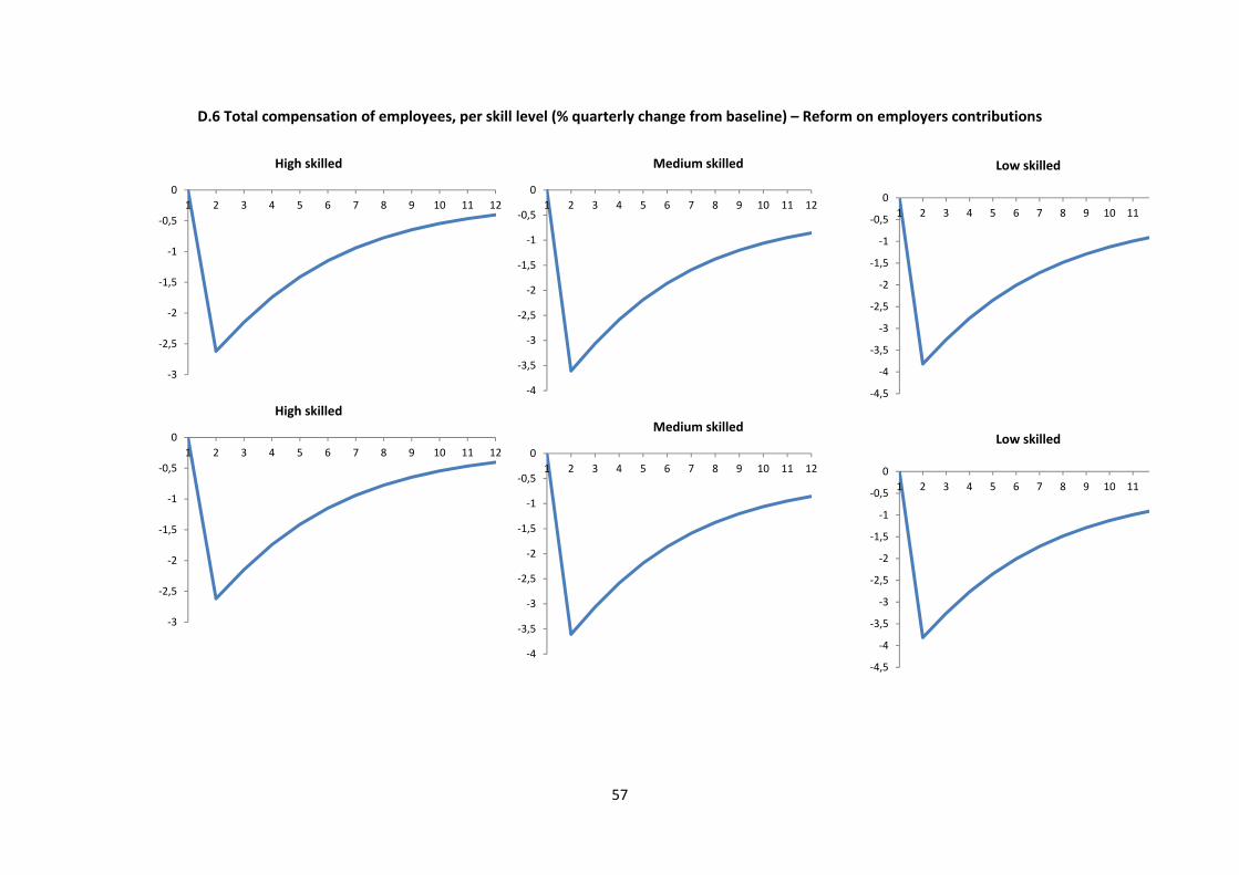
57  

D.6 Total compensation of employees, per skill level (% quarterly change from baseline) – Reform on employers contributions 

 

‐3

‐2,5

‐2

‐1,5

‐1

‐0,5

0

1 2 3 4 5 6 7 8 9 10 11 12

High skilled

‐3

‐2,5

‐2

‐1,5

‐1

‐0,5

0

1 2 3 4 5 6 7 8 9 10 11 12

High skilled

‐4

‐3,5

‐3

‐2,5

‐2

‐1,5

‐1

‐0,5

0

1 2 3 4 5 6 7 8 9 10 11 12

Medium skilled

‐4

‐3,5

‐3

‐2,5

‐2

‐1,5

‐1

‐0,5

0

1 2 3 4 5 6 7 8 9 10 11 12

Medium skilled

‐4,5

‐4

‐3,5

‐3

‐2,5

‐2

‐1,5

‐1

‐0,5

0

1 2 3 4 5 6 7 8 9 10 11

Low skilled

‐4,5

‐4

‐3,5

‐3

‐2,5

‐2

‐1,5

‐1

‐0,5

0

1 2 3 4 5 6 7 8 9 10 11

Low skilled

 

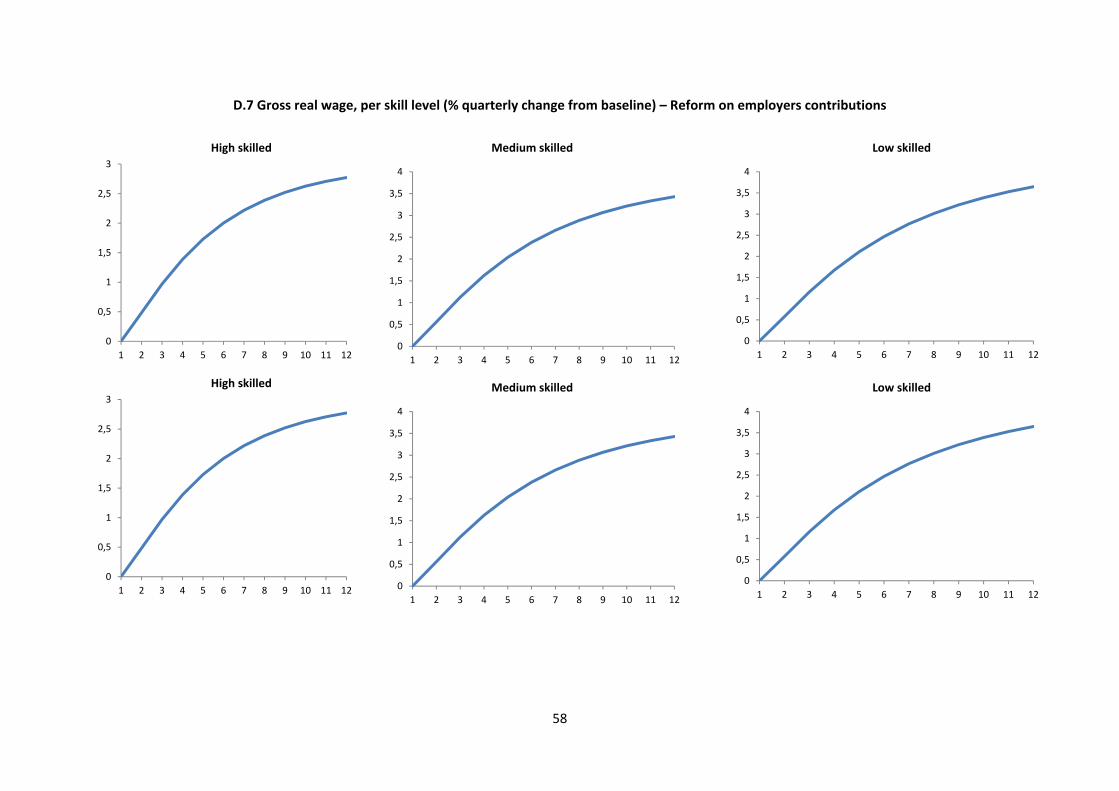
58  

D.7 Gross real wage, per skill level (% quarterly change from baseline) – Reform on employers contributions 

 

 

 

0

0,5

1

1,5

2

2,5

3

1 2 3 4 5 6 7 8 9 10 11 12

High skilled

0

0,5

1

1,5

2

2,5

3

1 2 3 4 5 6 7 8 9 10 11 12

High skilled

0

0,5

1

1,5

2

2,5

3

3,5

4

1 2 3 4 5 6 7 8 9 10 11 12

Medium skilled

0

0,5

1

1,5

2

2,5

3

3,5

4

1 2 3 4 5 6 7 8 9 10 11 12

Medium skilled

0

0,5

1

1,5

2

2,5

3

3,5

4

1 2 3 4 5 6 7 8 9 10 11 12

Low skilled

0

0,5

1

1,5

2

2,5

3

3,5

4

1 2 3 4 5 6 7 8 9 10 11 12

Low skilled

 

59  

D.8 Employment, per skill level (% quarterly change from baseline) – Reform on employers contributions 

   

0

0,1

0,2

0,3

0,4

0,5

0,6

0,7

0,8

0,9

1

1 2 3 4 5 6 7 8 9 10 11 12

High skilled

0

0,1

0,2

0,3

0,4

0,5

0,6

0,7

0,8

0,9

1

1 2 3 4 5 6 7 8 9 10 11 12

High skilled

0

0,2

0,4

0,6

0,8

1

1,2

1,4

1,6

1 2 3 4 5 6 7 8 9 10 11

Medium skilled

0

0,2

0,4

0,6

0,8

1

1,2

1,4

1,6

1 2 3 4 5 6 7 8 9 10 11

Medium skilled

0

0,2

0,4

0,6

0,8

1

1,2

1,4

1,6

1 2 3 4 5 6 7 8 9 10 11

Low skilled

0

0,2

0,4

0,6

0,8

1

1,2

1,4

1,6

1 2 3 4 5 6 7 8 9 10 11

Low skilled

 

60  

Appendix E. Budgetary and redistributive effects of the reforms E.1. Impact of the refundable tax credit reform on disposable income (by income decile) – Italy 

 

0%

1%

2%

2013 2014 2015 2016

Decile 1

0%

1%

2%

2013 2014 2015 2016

Decile 2

0%

1%

2%

2013 2014 2015 2016

Decile 3

0%

1%

2%

2013 2014 2015 2016

Decile 4

0%

1%

2%

2013 2014 2015 2016

Decile 5

0%

1%

2%

2013 2014 2015 2016

Decile 6

0%

1%

2%

2013 2014 2015 2016

Decile 7

0%

1%

2%

2013 2014 2015 2016

Decile 8

0%

1%

2%

2013 2014 2015 2016

Decile 9

0,0%

1,0%

2,0%

2013 2014 2015 2016

Decile 10

 

61  

E.2. Impact of the universal tax credit reform on disposable income (by income decile) – Poland 

 

0%

2%

5%

2013 2014 2015 2016

Decile 1

0%

2%

5%

2013 2014 2015 2016

Decile 2

0%

2%

5%

2013 2014 2015 2016

Decile 3

0%

2%

5%

2013 2014 2015 2016

Decile 4

0%

2%

5%

2013 2014 2015 2016

Decile 5

0%

2%

5%

2013 2014 2015 2016

Decile 6

0%

2%

5%

2013 2014 2015 2016

Decile 7

0%

2%

5%

2013 2014 2015 2016

Decile 8

0%

2%

5%

2013 2014 2015 2016

Decile 9

0%

2%

5%

2013 2014 2015 2016

Decile 10