Dynamic Scoring at CBO

Congressional Budget Office

Dynamic Scoring at CBO

NABE Foundation, 12th Annual Economic Measurement Seminar Four Seasons Hotel, Washington, D.C.

Ben Page Unit Chief, Fiscal Policy Studies

July 21, 2015

1 C O N G R E S S I O N A L B U D G E T O F F I C E

Overview

■ New requirement for dynamic scoring

■ CBO’s approach to analyzing effects of fiscal policy

■ Case study: A dynamic estimate of repealing the Affordable Care Act


The New Requirement for Dynamic Scoring


Main Points

■ The requirement to estimate the budgetary feedback of macroeconomic effects applies to major legislation

■ Conventional cost estimates already incorporate behavioral responses but not changes in broad economic variables

■ CBO has regularly done estimates of the budgetary feedback of macroeconomic effects but generally not for cost estimates for legislation


Requirements Under 2016 Budget Resolution

■ To the greatest extent practicable, CBO and JCT shall incorporate the budgetary effects of changes in macroeconomic variables resulting from legislation that – Has a gross budgetary effect of 0.25 percent of GDP in any year over the

next 10 years (an amount equal to about $45 billion in 2015) or

– Is designated by one of the Chairmen of the Budget Committees

■ Estimates shall also include a qualitative assessment of the budgetary effects (including macroeconomic effects) for the subsequent 20-year period

■ Appropriation acts are excluded

■ CBO and JCT will coordinate on legislation that significantly affects both spending and tax policies


Behavioral Responses Addressed in Conventional Cost Estimates

■ If proposed policies would affect people’s behavior in ways that would generate direct budgetary savings or costs, the effects are incorporated in CBO’s cost estimates – The change in production of various crops that would result from

adopting new farm policies – The likelihood that people would take up certain government benefits

if policies pertaining to those benefits were changed – The quantity of health care services that would be provided if

Medicare’s payment rates to providers were adjusted

■ By long-standing convention, CBO’s cost estimates generally have not reflected changes in behavior that would affect total output in the economy, such as any changes in labor supply or private investment resulting from changes in fiscal policy


The New Requirement Extends Previous Analyses by CBO

■ CBO has routinely produced estimates of the macroeconomic effects of fiscal policies and of the feedback from those macroeconomic changes to the federal budget – Analysis of the President’s budget – Annual long-term budget and economic outlook – Analyses of illustrative fiscal policy scenarios

■ CBO has generally not produced such estimates for specific legislation prior to the 2016 budget resolution. One exception: S. 744, the Border Security, Economic Opportunity, and Immigration Modernization Act – Because the bill would have significantly increased the size of the

U.S. labor force, CBO and JCT incorporated in the cost estimate their projections of the direct effects of the act on the U.S. population, employment, and taxable compensation

– CBO separately published analysis of additional economic effects and their feedback to the budget


CBO’s Approach to Dynamic Analysis


CBO’s Approach to Analyzing Economic Effects of Fiscal Policies

■ Short term: Changes in fiscal policies affect the overall economy primarily by influencing the demand for goods and services by consumers, businesses, and governments, which leads to changes in output relative to potential (maximum sustainable) output

■ Long term: Changes in fiscal policies affect output primarily by altering national saving, federal investment, and people’s incentives to work and save, as well as businesses’ incentives to invest, thereby changing potential output


Central Estimates and Ranges

■ CBO’s estimates of those effects are based on parameters such as the extent to which national saving is altered by changes in fiscal policies

■ In most cases, CBO estimates the economic effects (and feedback to the budget) using a range of parameter estimates reflecting the consensus in the economic literature

■ To arrive at its estimate of the economic effects, CBO uses the central estimates for those parameters


Short-Term Effects From Changes in Demand

■ Direct contributions to aggregate demand from changes in purchases by federal agencies and those who receive federal payments and pay taxes

■ The change in output for each dollar of direct contribution to demand (the “demand multiplier”) varies with the response of monetary policy

■ In CBO’s estimates of indirect effects: – When the monetary policy response is likely to be limited, the demand

multiplier over four quarters ranges from 0.5 to 2.5, with a central estimate of 1.5

– When the monetary policy response is likely to be stronger, the demand multiplier over four quarters ranges from 0.4 to 1.9, with a central estimate of 1.2; over eight quarters, it ranges from 0.2 to 0.8, with a central estimate of 0.5


Short-Term Effects From Changes in Labor Supply

■ Effects on the supply of labor lead to changes in employment, depending on the amount of slack in the labor market


Long-Term Effects

■ CBO uses two models of potential output to estimate the effects of changes in fiscal policies on the overall economy over the long term – Solow-type growth model – Life-cycle growth model

■ Potential output depends on – Amount and quality of labor and capital (which depend on work,

saving, and investment) – Productivity of the labor and capital inputs (which depends in part on

federal investment) – Amount of national saving (which depends in part on federal

borrowing)


The Role of Expectations About Fiscal Policy

■ Solow-type growth model – People base their decisions about working and saving primarily on

current economic conditions, including government policies – Decisions reflect people’s anticipation of future policies in a general

way but not their responses to specific future developments

■ Life-cycle growth model – People make choices about working and saving in response to both

current economic conditions and their explicit expectations of future economic conditions

– The model requires specification of future fiscal policies that put federal debt on a sustainable path over the long run because forward-looking households would not hold government bonds if the households expected that debt as a percentage of GDP would rise without limit


How Labor Supply Responds to Changes in Fiscal Policy in the Solow-Type Growth Model

■ The overall effects of a policy change on the labor supply can be expressed as an elasticity, which is the percentage change in the labor supply resulting from a 1 percent change in after-tax income – Substitution effect: Increased after-tax compensation for an additional

hour of work makes work more valuable relative to other uses of a person’s time

– Income effect: Increased after-tax income from a given amount of work allows people to maintain the same standard of living while working fewer hours


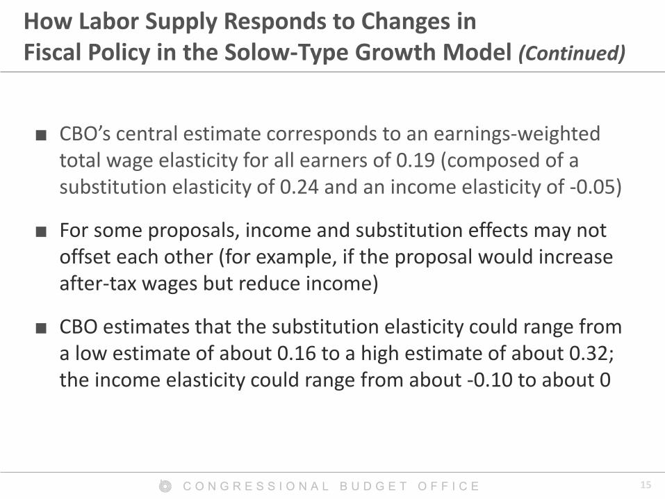
How Labor Supply Responds to Changes in Fiscal Policy in the Solow-Type Growth Model (Continued)

■ CBO’s central estimate corresponds to an earnings-weighted total wage elasticity for all earners of 0.19 (composed of a substitution elasticity of 0.24 and an income elasticity of -0.05)

■ For some proposals, income and substitution effects may not offset each other (for example, if the proposal would increase after-tax wages but reduce income)

■ CBO estimates that the substitution elasticity could range from a low estimate of about 0.16 to a high estimate of about 0.32; the income elasticity could range from about -0.10 to about 0


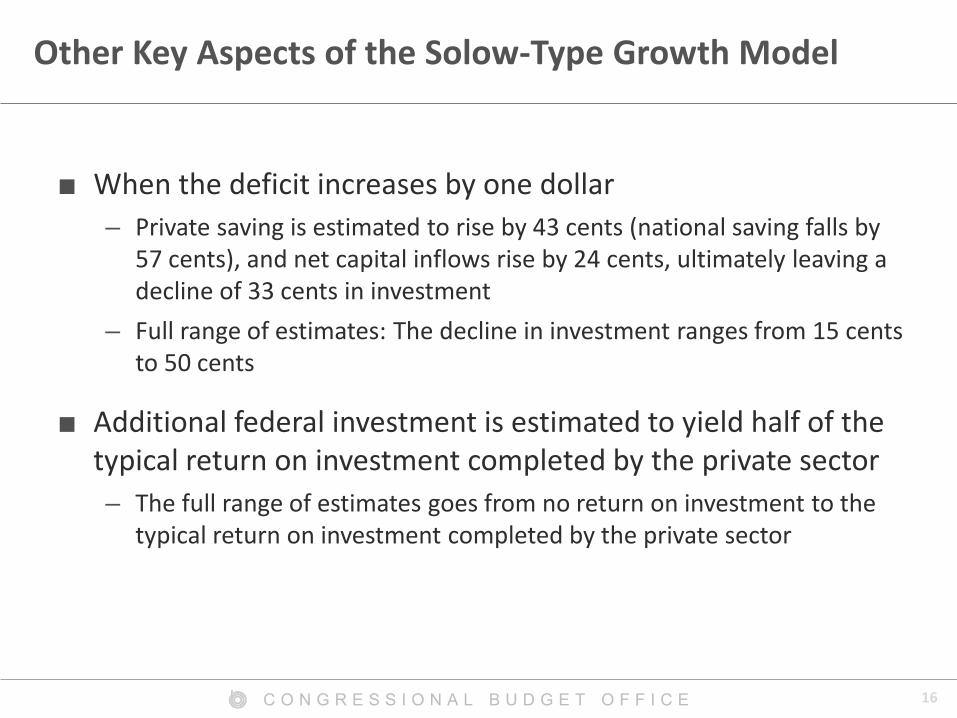
Other Key Aspects of the Solow-Type Growth Model

■ When the deficit increases by one dollar – Private saving is estimated to rise by 43 cents (national saving falls by

57 cents), and net capital inflows rise by 24 cents, ultimately leaving a decline of 33 cents in investment

– Full range of estimates: The decline in investment ranges from 15 cents to 50 cents

■ Additional federal investment is estimated to yield half of the typical return on investment completed by the private sector – The full range of estimates goes from no return on investment to the

typical return on investment completed by the private sector


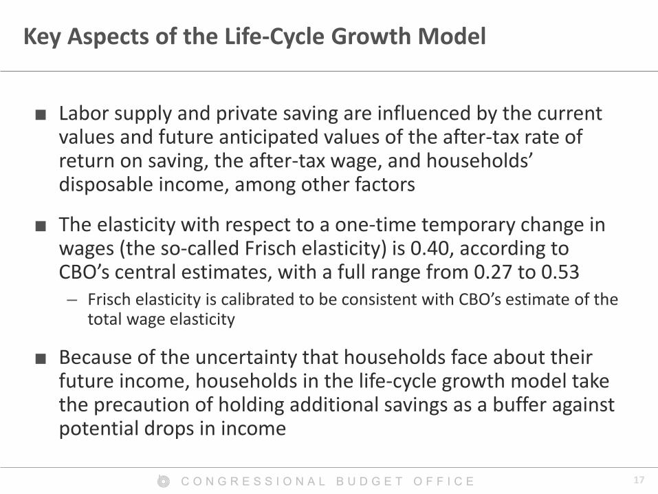
Key Aspects of the Life-Cycle Growth Model

■ Labor supply and private saving are influenced by the current values and future anticipated values of the after-tax rate of return on saving, the after-tax wage, and households’ disposable income, among other factors

■ The elasticity with respect to a one-time temporary change in wages (the so-called Frisch elasticity) is 0.40, according to CBO’s central estimates, with a full range from 0.27 to 0.53 – Frisch elasticity is calibrated to be consistent with CBO’s estimate of the

total wage elasticity

■ Because of the uncertainty that households face about their future income, households in the life-cycle growth model take the precaution of holding additional savings as a buffer against potential drops in income


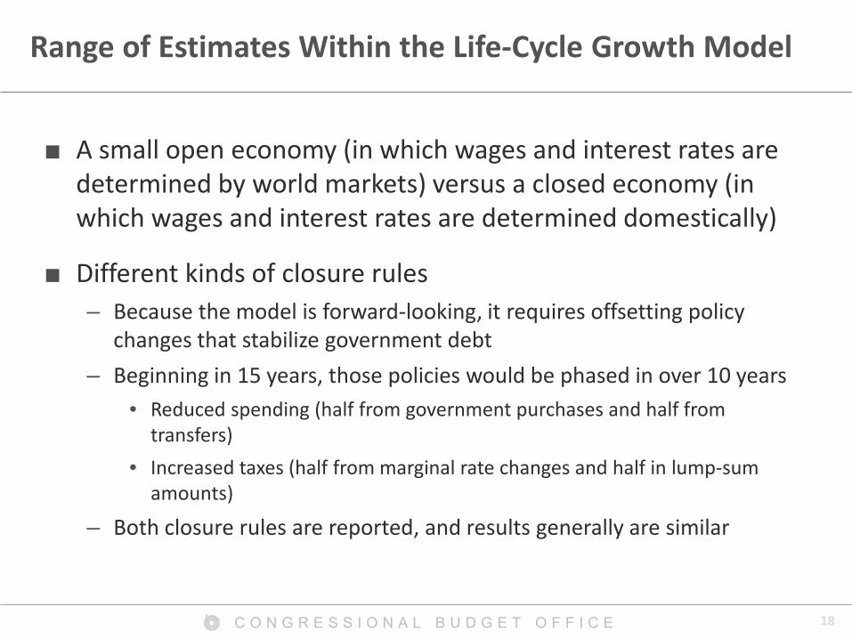
Range of Estimates Within the Life-Cycle Growth Model

■ A small open economy (in which wages and interest rates are determined by world markets) versus a closed economy (in which wages and interest rates are determined domestically)

■ Different kinds of closure rules – Because the model is forward-looking, it requires offsetting policy

changes that stabilize government debt – Beginning in 15 years, those policies would be phased in over 10 years

• Reduced spending (half from government purchases and half from transfers)

• Increased taxes (half from marginal rate changes and half in lump-sum amounts)

– Both closure rules are reported, and results generally are similar


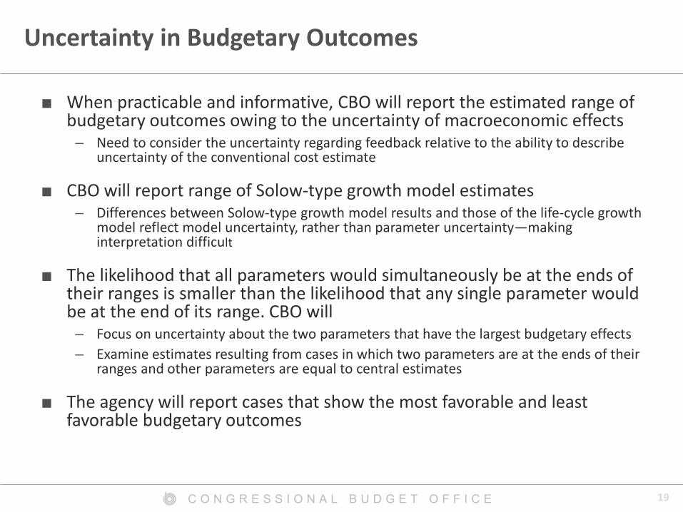
Uncertainty in Budgetary Outcomes

■ When practicable and informative, CBO will report the estimated range of budgetary outcomes owing to the uncertainty of macroeconomic effects

– Need to consider the uncertainty regarding feedback relative to the ability to describe uncertainty of the conventional cost estimate

■ CBO will report range of Solow-type growth model estimates – Differences between Solow-type growth model results and those of the life-cycle growth

model reflect model uncertainty, rather than parameter uncertainty—making interpretation difficult

■ The likelihood that all parameters would simultaneously be at the ends of their ranges is smaller than the likelihood that any single parameter would be at the end of its range. CBO will

– Focus on uncertainty about the two parameters that have the largest budgetary effects – Examine estimates resulting from cases in which two parameters are at the ends of their

ranges and other parameters are equal to central estimates

■ The agency will report cases that show the most favorable and least favorable budgetary outcomes


Presentation of Macroeconomic Analyses in Cost Estimates

■ Presentation will probably evolve over time as CBO learns what is most useful

■ Estimates will show all of the information that traditionally would be included if macroeconomic effects were not incorporated and will identify the macroeconomic effects separately

■ Estimates will provide information related to the uncertainty of the macroeconomic effects


Case Study: A Dynamic Estimate of Repealing the Affordable Care Act


Conclusions

■ Analysis used long-standing procedures, models, and estimates—but applied them in a new way

■ There is substantial uncertainty about budgetary effects and macroeconomic feedbacks

■ Over the next decade, the uncertainty is large enough that repealing the ACA could reduce cumulative deficits—or increase them by much more than estimated

■ ACA repeal includes large offsetting changes to spending and revenues

■ In CBO’s analyses of other policies, macroeconomic feedback has been less significant relative to the estimated cost without macroeconomic feedback


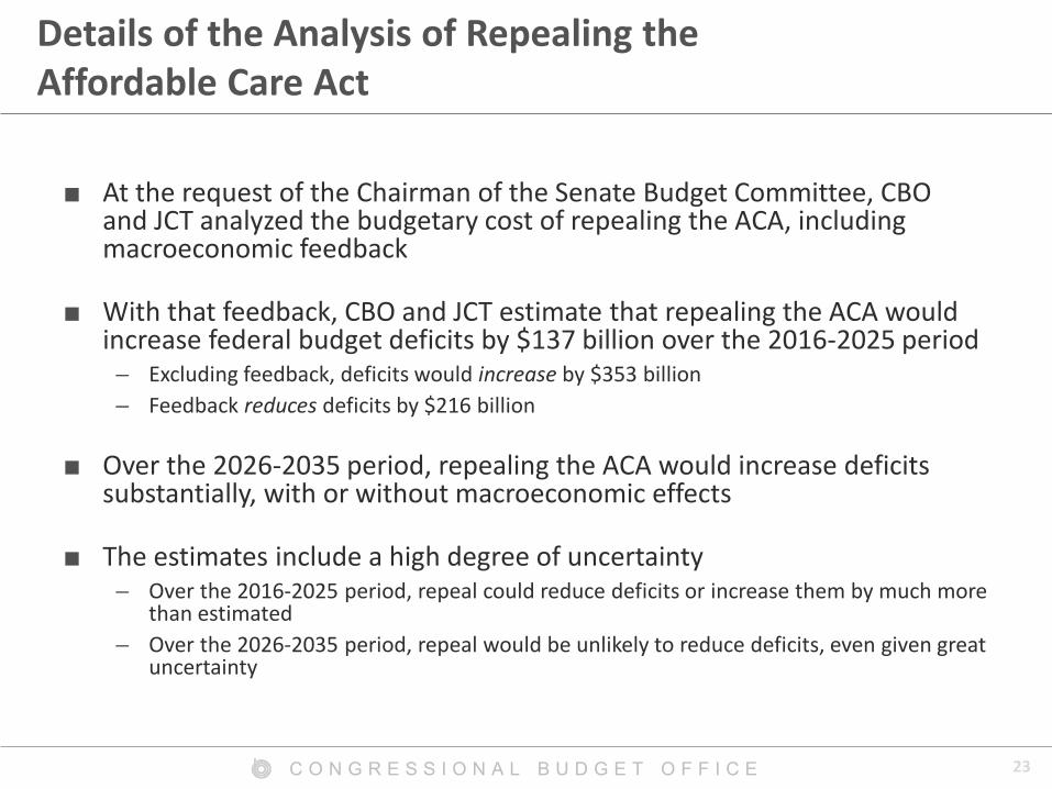
Details of the Analysis of Repealing the Affordable Care Act

■ At the request of the Chairman of the Senate Budget Committee, CBO and JCT analyzed the budgetary cost of repealing the ACA, including macroeconomic feedback

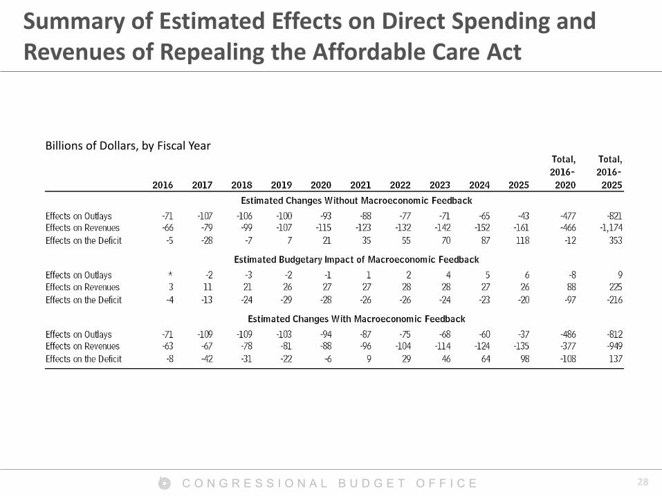
■ With that feedback, CBO and JCT estimate that repealing the ACA would increase federal budget deficits by $137 billion over the 2016-2025 period

– Excluding feedback, deficits would increase by $353 billion – Feedback reduces deficits by $216 billion

■ Over the 2026-2035 period, repealing the ACA would increase deficits substantially, with or without macroeconomic effects

■ The estimates include a high degree of uncertainty – Over the 2016-2025 period, repeal could reduce deficits or increase them by much more

than estimated – Over the 2026-2035 period, repeal would be unlikely to reduce deficits, even given great

uncertainty


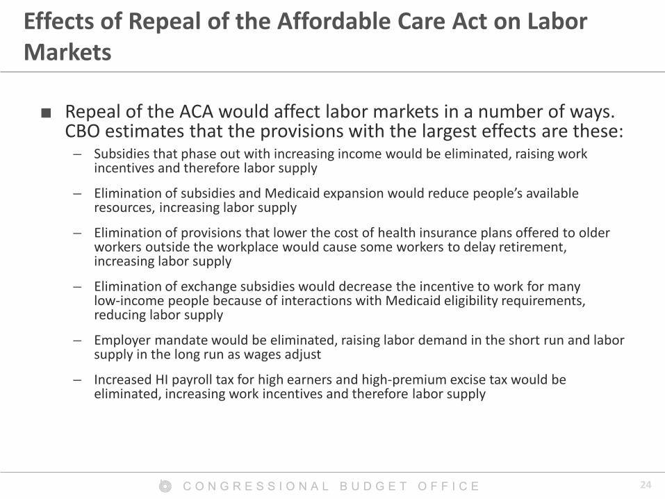
Effects of Repeal of the Affordable Care Act on Labor Markets

■ Repeal of the ACA would affect labor markets in a number of ways. CBO estimates that the provisions with the largest effects are these:

– Subsidies that phase out with increasing income would be eliminated, raising work incentives and therefore labor supply

– Elimination of subsidies and Medicaid expansion would reduce people’s available resources, increasing labor supply

– Elimination of provisions that lower the cost of health insurance plans offered to older workers outside the workplace would cause some workers to delay retirement, increasing labor supply

– Elimination of exchange subsidies would decrease the incentive to work for many low-income people because of interactions with Medicaid eligibility requirements, reducing labor supply

– Employer mandate would be eliminated, raising labor demand in the short run and labor supply in the long run as wages adjust

– Increased HI payroll tax for high earners and high-premium excise tax would be eliminated, increasing work incentives and therefore labor supply


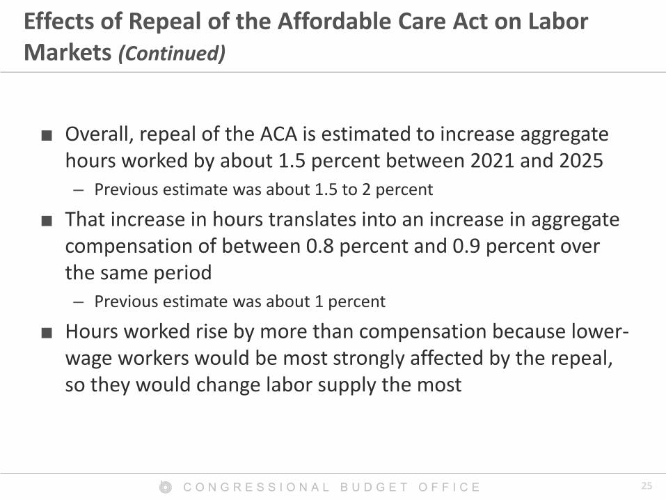
Effects of Repeal of the Affordable Care Act on Labor Markets (Continued)

■ Overall, repeal of the ACA is estimated to increase aggregate hours worked by about 1.5 percent between 2021 and 2025 – Previous estimate was about 1.5 to 2 percent

■ That increase in hours translates into an increase in aggregate compensation of between 0.8 percent and 0.9 percent over the same period – Previous estimate was about 1 percent

■ Hours worked rise by more than compensation because lower-wage workers would be most strongly affected by the repeal, so they would change labor supply the most


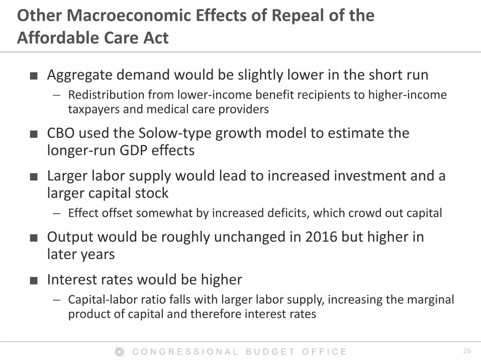
Other Macroeconomic Effects of Repeal of the Affordable Care Act

■ Aggregate demand would be slightly lower in the short run – Redistribution from lower-income benefit recipients to higher-income

taxpayers and medical care providers

■ CBO used the Solow-type growth model to estimate the longer-run GDP effects

■ Larger labor supply would lead to increased investment and a larger capital stock – Effect offset somewhat by increased deficits, which crowd out capital

■ Output would be roughly unchanged in 2016 but higher in later years

■ Interest rates would be higher – Capital-labor ratio falls with larger labor supply, increasing the marginal

product of capital and therefore interest rates


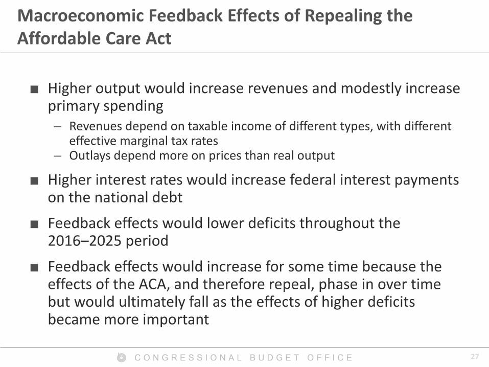
Macroeconomic Feedback Effects of Repealing the Affordable Care Act

■ Higher output would increase revenues and modestly increase primary spending – Revenues depend on taxable income of different types, with different

effective marginal tax rates – Outlays depend more on prices than real output

■ Higher interest rates would increase federal interest payments on the national debt

■ Feedback effects would lower deficits throughout the 2016–2025 period

■ Feedback effects would increase for some time because the effects of the ACA, and therefore repeal, phase in over time but would ultimately fall as the effects of higher deficits became more important


Summary of Estimated Effects on Direct Spending and Revenues of Repealing the Affordable Care Act

Billions of Dollars, by Fiscal Year


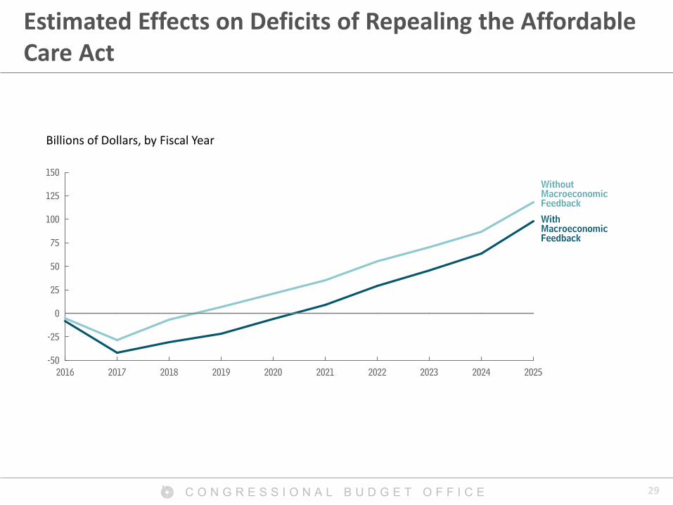
Estimated Effects on Deficits of Repealing the Affordable Care Act

2016 2017 2018 2019 2020 2021 2022 2023 2024 2025-50

-25

0

25

50

75

100

125

150WithoutMacroeconomicFeedback

WithMacroeconomicFeedback

Billions of Dollars, by Fiscal Year


Additional Resources

■ Answers to Questions for the Record Following a Hearing on the Budget and Economic Outlook for 2015 to 2025 Conducted by the House Committee on the Budget (March 2015), www.cbo.gov/publication/49975

■ Macroeconomic Analysis of Legislative Proposals (May 2013), www.cbo.gov/publication/44165

■ How CBO Analyzes the Effects of Changes in Federal Fiscal Policies on the Economy (November 2014), www.cbo.gov/publication/49494

■ Budgetary and Economic Effects of Repealing the Affordable Care Act (June 2015), www.cbo.gov/publication/50252

■ The Budget and Economic Outlook: 2014 to 2024 (February 2014), Appendix C (pp. 117-127), www.cbo.gov/publication/45010

■ The Economic Effects of the President’s 2015 Budget (July 2014), www.cbo.gov/publication/45540

http://www.cbo.gov/publication/49975






Government & Nonprofit

Dynamic Scoring at CBO